Ar

Ra

b

c

d

a

ARRAA

KHERTP

1

anbbsitel0aTp

AL

1d

Biomedical Signal Processing and Control 5 (2010) 299–310

Contents lists available at ScienceDirect

Biomedical Signal Processing and Control

journa l homepage: www.e lsev ier .com/ locate /bspc

nalysis of heart rate variability during exercise stress testing usingespiratory information

aquel Bailóna,b,∗, Luca Mainardic, Michele Orinia,b,c, Leif Sörnmod, Pablo Lagunaa,b

Communications Technology Group (GTC) at the Aragón Institute of Engineering Research (I3A), University of Zaragoza, María de Luna 1, 50018 Zaragoza, SpainCIBER de Bioingeniería, Biomateriales y Nanomedicina (CIBER-BBN), SpainDepartment of Bioengineering, Politecnico di Milano, via Golgi 39, 20133 Milano, ItalySignal Processing Group, Department of Electrical and Information Technology, Lund University, Lund, Sweden

r t i c l e i n f o

rticle history:eceived 8 January 2010eceived in revised form 19 April 2010ccepted 17 May 2010vailable online 18 June 2010

eywords:eart rate variabilityxercise stress testing

a b s t r a c t

This paper presents a novel method for the analysis of heart rate variability (HRV) during exercise stresstesting enhanced with respiratory information. The instantaneous frequency and power of the low fre-quency (LF) and high frequency (HF) bands of the HRV are estimated by parametric decomposition ofthe instantaneous autocorrelation function (ACF) as a sum of damped sinusoids. The instantaneous ACFis first windowed and filtered to reduce the cross terms. The inclusion of respiratory information is pro-posed at different stages of the analysis, namely, the design of the filter applied to the instantaneousACF, the parametric decomposition, and the definition of a dynamic HF band. The performance of themethod is evaluated on simulated data as well as on a stress testing database. The simulation results

espiratory frequencyime–frequency analysisarametric decomposition

show that the inclusion of respiratory information reduces the estimation error of the amplitude of theHF component from 3.5% to 2.4% in mean and related SD from 3.0% to 1.7% when a tuned time smoothingwindow is used at an SNR of 15 dB. Results from the stress testing database show that information onrespiratory frequency produces HF power estimates which closely resemble those from the simulationswhich exhibited lower SD. The mean SD of these estimates with respect to their mean trends is reducedby 84% (from 0.74 × 10−3 s−2 to 0.12 × 10−3 s−2). The analysis of HRV in the stress testing database reveals

he po

a significant decrease in t

. Introduction

Spectral analysis of heart rate variability (HRV) is widely useds a non-invasive technique for the assessment of the auto-omic nervous system (ANS) activity on the heart and the balanceetween the sympathetic and parasympathetic systems [1]. Thisalance may be altered under certain pathological conditions,uch as myocardial infarction, diabetic neuropathy [1], and cardiacschemia [2,3]. Standards of measurement, physiological interpre-ation and clinical use of HRV in resting conditions have beenstablished, involving three different spectral components: a veryow frequency (VLF) component in the range between 0 and

.04 Hz, a low frequency (LF) component between 0.04 and 0.15 Hz,nd a high frequency (HF) component between 0.15 and 0.4 Hz [1].he power in the HF band is considered to be a measure of parasym-athetic activity, mainly due to respiratory sinus arrhythmia (RSA).

∗ Corresponding author at: Communications Technology Group (GTC) at theragón Institute of Engineering Research (I3A), University of Zaragoza, María deuna 1, Ed. Ada Byron, 50018 Zaragoza, Spain.

E-mail address: rbailon@unizar.es (R. Bailón).

746-8094/$ – see front matter © 2010 Elsevier Ltd. All rights reserved.oi:10.1016/j.bspc.2010.05.005

wer of both the LF and HF components around peak stress.© 2010 Elsevier Ltd. All rights reserved.

The power in the LF band is considered to be a measure of sympa-thetic and parasympathetic activity, together with other regulatorymechanisms such as the rennin–angiotensin system and baroreflex[4], its interpretation being controversial when, e.g. the respiratoryfrequency lies in the LF band.

Certain indices of HRV analysis during exercise stress testinghave shown added value in the diagnosis of coronary artery dis-ease [5]. The analysis of HRV during stress testing is challengingdue to the non-stationary recording conditions. The factors whichinfluence HRV during spontaneous conditions [6] are altered duringexercise [7]. Several approaches to non-stationary analysis of HRVhave been proposed in the literature [8], of which time–frequency(TF) analysis is the most common. This approach can be dividedinto three categories: (i) non-parametric methods based on lin-ear filtering, including the short-time Fourier transform [9–11]and the wavelet transform [12–14], (ii) non-parametric quadraticTF representations, including the Wigner–Ville distribution and

its filtered versions [15–17], and (iii) parametric methods basedon autoregressive models with time-varying coefficients [18,10].The smoothed pseudo Wigner–Ville distribution (SPWVD) providesbetter resolution than non-parametric linear methods, indepen-dent control of time and frequency filtering, and power estimates

3 rocess

wocic

ttmaospnhat

sniqrfLt

ttftfaavaaiatr

2

HosamcsAvsesb

2

sss

00 R. Bailón et al. / Biomedical Signal P

ith lower variance than parametric methods when rapid changesccur [16,19]. The main drawback of the SPWVD is the presence ofross terms, which can be attenuated by time and frequency filter-ng. In this work an approach for overcoming this drawback in theontext of HRV analysis during stress testing is considered.

The coupling between the cardiovascular and respiratory sys-ems results in modulation of the heart rate, i.e. RSA, mainly dueo parasympathetic activity at rest [20–22]. However, the use of

easures extracted from the RSA as indices of parasympatheticctivity during exercise is questionable. During exercise, inhibitionf the parasympathetic activity is followed by an increase in theympathetic activity at high work loads [23,7]. According to thearasympathetic withdrawal, the RSA decreases from the begin-ing of the exercise, whereas an increase in RSA is observed duringigh work loads which cannot be explained by parasympatheticctivity. This increase can be attributed to mechanical stretching ofhe sinus node in response to a ventilation increase [24,25].

The fact that respiratory frequency is not restricted to the clas-ical HF band [0.15, 0.4] Hz during exercise stress testing makes itecessary to redefine the HF band [26]. In some studies, the HF band

s extended to include the whole range of possible respiratory fre-uencies [27,28,9,29,13], the upper limit being half the mean heartate (HR). In other cases, the HF band is centered on the respiratoryrequency with constant or time-dependent bandwidth [14]. TheF band can be redefined to range from its lower limit (i.e. 0.04 Hz)o the lower limit of the HF band.

In this paper, a method for HRV analysis during exercise stressesting is presented which makes use of information on respira-ory frequency. The objective of this work is to propose a methodor HRV analysis during stress testing which makes use of informa-ion on respiratory frequency when estimating the instantaneousrequency and power of the LF and HF components. The method isn extension of the parametric decomposition of the instantaneousutocorrelation function (ACF) on which the SPWVD is based, pre-iously applied to analysis of HRV during tilt test [17]. The methodssumes that the instantaneous ACF of the HRV can be decomposed,t each time instant, as a sum of damped sinusoids from which thenstantaneous frequency and power of the LF and HF componentsre derived. The methods are presented in Section 2, the simula-ion study and the exercise stress testing database in Section 3, theesults in Section 4 and, finally, a discussion is found in Section 5.

. Methods

The estimation of the instantaneous frequency and power of theRV components is performed in three steps: (i) the computationf the windowed and filtered instantaneous ACF of the HRV analyticignal, (ii) its parametric decomposition to obtain the instantaneousmplitude and frequency of the HRV components, and (iii) the esti-ation of the instantaneous frequency and power of the LF and HF

omponents. The inclusion of respiratory information will be con-idered for: (i) adapting the time smoothing window that filters theCF in order to make estimation errors independent of the rate ofariation of respiratory frequency, (ii) constraining the decompo-ition of the instantaneous ACF in order to reduce the estimationrror, and (iii) dynamic definition of the HF band in order to con-ider respiratory frequencies that may be outside the standard HFand. The method is described by the block diagram shown in Fig. 1.

.1. Model of heart rate variability during stress testing

Heart rate variability may be modeled as a sum of two or moreinusoids whose frequencies vary linearly in time [17]. Duringtress testing, the LF and HF components are represented by twoinusoids which are embedded in additive white Gaussian noise

ing and Control 5 (2010) 299–310

(AWGN). The analytic HRV signal x(n) may be modeled as

x(n) = ALF(n)ej2�fLFn + AHF(n)ej2�(˛n2+ˇn) + v(n). (1)

The LF component is defined by the amplitude ALF(n) and the dis-crete frequency fLF, assumed to be constant during the stress test.The HF component is defined by the amplitude AHF(n) and theinstantaneous discrete frequency fHF(n) = 2˛n + ˇ, where 2˛ rep-resents the slope of fHF(n) and ˇ the intercept; thus, the frequencyis assumed to increase linearly with work load until peak stressand then decrease linearly during recovery [25,30]. The discretefrequencies are related to the analog frequencies through the sam-pling rate Fs (FLF = fLFFs, FHF = fHFFs, respectively). The term v(n)represents the analytic signal of the AWGN, which accounts forjitter in the QRS fiducial point as well as for modeling inaccuracies.

It is assumed that the variations in the LF and HF amplitudesare slow compared to the LF and HF oscillations, respectively, sothat the “quasi-stationary” condition is fulfilled [31]. As a result,the model in (1) can be simplified so that, locally, ALF(n) � ALF andAHF(n) � AHF.

The VLF component is not considered in this model since it can-not be estimated during stress testing.

2.2. The instantaneous autocorrelation function

The discrete SPWVD of a real-valued discrete-time signal, whoseanalytic version is x(n), is defined by [32,33,31]

Px(n, m) = 2K−1∑

k=−K+1

|h(k)|2[

N−1∑n′=−N+1

g(n′)x(n + n′ + k)x∗(n + n′ − k)

]

× e−j2�(m/M)k; m = −M + 1, . . . , M, (2)

where n and m are the time and frequency indices, respectively.The term g(n′) is a symmetric time smoothing window of length2N − 1. The term |h(k)|2 is a symmetric frequency smoothing win-dow of length 2K − 1 (2K − 1 < 2M). In order to conserve theenergy the time and frequency windows are normalized so that∑N−1

n′=−N+1g(n′) = 1 and |h(0)|2 = 1, respectively.The distribution Px(n, m/2) can be viewed as the discrete Fourier

transform of rx(n, k), which is the instantaneous ACF x(n + k)x∗(n −k) filtered by g(n′) and windowed by |h(k)|2,

rx(n, k) = |h(k)|2[

N−1∑n′=−N+1

g(n′)x(n + n′ + k)x∗(n + n′ − k)

]. (3)

We will now derive the ACF for the model in (1). The instantaneousACF of x(n) is given by

x(n + k)x∗(n − k) = |ALF|2ej2�fLF2k + |AHF|2ej2�fHF(n)2k

+ 2R{ALFA∗HF} cos

[2�(˛(n2 + k2) + (ˇ − fLF)n)

]× ej2�(fLF+fHF(n))k + w(n + k)w∗(n − k),

(4)

where the term w(n + k)w∗(n − k) accounts for all the noise con-tributions, including v(n + k)v∗(n − k) as well as the cross productsbetween the signal components and the noise. Using a rectangularwindow for time smoothing [17]

g(n′) ={ 1

2N − 1, n′ = −N + 1, . . . , N − 1

0, otherwise,(5)

and an exponential window for frequency smoothing

|h(k)|2 ={

e−� |k|, k = −K + 1, . . . , K − 10, otherwise,

(6)

R. Bailón et al. / Biomedical Signal Processing and Control 5 (2010) 299–310 301

F lytic Ha ), FLF(c

tf

Dctsi2o

2

bdsitsttdtcd

nu

r

Ft01

ig. 1. Block diagram of the method for HRV analysis, where x(n) stands for the anare the instantaneous amplitude and frequency of the HRV components, and PLF(nomponents, respectively.

he windowed and filtered ACF rx(n, k) becomes (see Appendix Aor derivation)

rx(n, k) = |ALF|2e−� |k|ej2�fLF2k + 12N − 1

|AHF|2e−� |k| sin(2�2˛(2N − 1)k)sin(2�2˛k)

ej2�fHF(n)2k

+ 12N − 1

2R{ALFA∗HF}e−� |k|

(N−1∑

n′=−N+1

c(n, n′, k)ej2�2˛n′k

)

× ej2�(fLF+fHF(n))k + rw(n, k).

(7)

ue to time smoothing, the amplitude and bandwidth of the HFomponent depend on 2˛ and 2N − 1 (see (7)). Note that the ampli-ude of the cross term can be considerably reduced by properelection of 2N − 1. In Fig. 2, Px(n, m) is displayed for two timenstants n1 and n2 with identical instantaneous frequency but with|˛2| > 2|˛1|. The HF peak at n1 is higher and narrower than thene at n2.

.3. Parameter estimation

The estimation of FLF(n), ALF(n), FHF(n), and AHF(n) is addressedy the parametric decomposition of rx(n, k) in (7)[17], which can beecomposed for each time instant n into a sum of complex dampedinusoids plus noise. In fact, the term related to the LF components in itself a complex damped sinusoid, whereas the term relatedo the HF component can be approximated by a complex dampedinusoid provided that the damping parameter � is large enougho attenuate the lobes of the term sin(2�2˛(2N − 1)k)/ sin(2�2˛k);he interference term is assumed to be small, as illustrated in Fig. 2,ue to the use of (5) and (6), and is included in the noise term. Notehat, although the parameters FLF, ALF and AHF have been assumedonstant for the derivation of rx(n, k), their estimation is madeependent on n since they are estimated for each time instant.

The function rx(n, k) is assumed to consist of a time-varyingumber I(n) of complex damped sinusoids corrupted by AWGN

(n, k),

x(n, k)=I(n)∑i=1

Ci(n)e(−�i(n)+jωi(n))k + u(n, k), k = 0, 1, . . . , K − 1, (8)

ig. 2. The SPWVD Px(n, m) for two time instants, n1 (solid line) correspondso 250 s, and n2 (dashed line) corresponds to 817 s, such as FLF(n1) = FLF(n2) =.1 Hz, FHF(n1) = FHF(n2) = 0.42 Hz, 2|˛1|Fs = 1.67 × 10−4 Hz/s and 2|˛2|Fs = 5.00 ×0−4 Hz/s. Note the reduced amplitude of the interference terms.

RV signal, rx(n, k) is the windowed and filtered instantaneous ACF, Ai(n) and Fi(n)n), PHF(n) and FHF(n) are the instantaneous power and frequency of the LF and HF

where u(n, k) includes the noise term rv(n, k), the interference term(i.e., third term in (7)), and modeling inaccuracies. Once the param-eters ωi(n) and Ci(n) of the I(n) complex damped sinusoids areestimated, the instantaneous amplitude and frequency of LF and HFcomponents can be derived. Note that I(n) = 2 for all time instantswhen the model in (1) is assumed. However, a time-varying num-ber of sinusoids I(n) is considered so as to account for the fact thatmore than two components usually exist in HRV signals. For exam-ple, a pedalling component is sometimes present in stress testingin addition to the LF and HF components [34].

The parameters Ci(n), �i(n) and ωi(n) are estimated using asuboptimal least-squares (LS) approach in which the propertiesof a prediction error filter polynomial Bn(z) = 1 + b(n, 1)z−1 +b(n, 2)z−2 + . . . + b(n, P)z−P are explored [35]. In the absence ofnoise the following linear prediction equation of order P shouldbe fulfilled,

Rx(n)b(n) = −rx(n), (9)

where

Rx(n) =

⎡⎢⎢⎢⎢⎣

r∗x (n, 1) r∗

x (n, 2) . . . r∗x (n, P)

r∗x (n, 2) r∗

x (n, 3) . . . r∗x (n, P + 1)

......

...

r∗x (n, K − P) r∗

x (n, K − P + 1) . . . r∗x (n, K − 1)

⎤⎥⎥⎥⎥⎦ (10)

b(n) = [b(n, 1)b(n, 2) . . . b(n, P)]T ,

rx(n) = [r∗x (n, 0)r∗

x (n, 1) . . . r∗x (n, K − P − 1)]T .

It can be shown that, in the absence of noise, Bn(z) has zeros atzi(n) = e(�i(n)+jωi(n)), if P is chosen so as to satisfy I(n) ≤ P ≤ K − I(n)[36].

In the presence of noisy data b(n) can be estimated in the LSsense by minimizing

Jn = (rx(n) + Rx(n)b(n))H(rx(n) + Rx(n)b(n)), (11)

resulting in

b(n) = −(RHx (n)Rx(n))

−1RH

x (n)rx(n). (12)

The inaccuracies in b(n) introduced by the presence of the noiseu(n, k) can be alleviated by substituting Rx(n) with its truncatedsingular value decomposition (SVD) Rx(n), where the smallest sin-gular values of Rx(n) are set to zero [35]. In this study the singularvalues smaller than 10% of the largest singular value are set to zeroand, accordingly, the number of complex damped sinusoids I(n) canbe estimated directly as the rank of Rx(n).

The parameters �i(n) and ωi(n) can be derived from the zeros ofBn(z),

�i(n) = R{ln(zi(n))}, ωi(n) = I{ln(zi(n))}, (13)

and, after replacing their estimates in (8), the parameters Ci(n) canbe obtained as the LS solution of the linear system. Then, the ampli-tude and frequency of the complex sinusoids of x(n) can be obtained

3 rocess

a

F

ThH

F

F

wd

c

A

2

pitpoa.

c

wpt

Tt

IetreH

O1eaıewtboo

o

02 R. Bailón et al. / Biomedical Signal P

s

i(n) = 12

ωi(n)2�

Fs, Ai(n) =√

|Ci(n)|. (14)

he LF and HF components can be chosen as the two sinusoids withighest power whose estimated frequency Fi(n) lies in the LF andF band, respectively.

ˆLF(n) = argmaxFi ∈ �LFAi(n), ALF(n) = maxFi ∈ �LF

Ai(n), (15)

ˆHF(n) = argmaxFi ∈ �HFAi(n), AHF(n) = maxFi ∈ �HF

Ai(n), (16)

here �LF and �HF represent the LF and HF bands, respectively,efined in Section 2.6. The instantaneous power of the LF and HF

omponents can be estimated as PLF(n) = A2LF(n)/2 and PHF(n) =

ˆ2HF(n)/2, respectively.

.4. Inclusion of information on respiratory frequency

It is now assumed that FHF(n) can be approximated by the res-iratory frequency. Then, respiratory information can be included

n the estimation of the HRV components. Suppose that the zero ofhe prediction error filter polynomial associated with the HF com-onent, zHF(n), is known (see later for details), then the estimationf b(n) can be solved as a constrained LS problem. Since zHF(n) iszero of Bn(z) it holds that Bn(zHF) = 1 + b(n, 1)z−1

HF + b(n, 2)z−2HF +

. . + b(n, P)z−PHF = 0, so the constraint can be expressed as

(b(n)) = bT (n)zHF(n) + 1 = 0, (17)

here zHF(n) =[z−1

HF (n), z−2HF (n), . . . , z−P

HF (n)]T

. The constrained LSroblem can be solved by using Lagrange multipliers; the functiono be minimized is

Jc,n = Jn + R{

c(b(n))�∗} . (18)

he constrained LS estimator is given by (see Appendix B for deriva-ion)

bc(n) = b(n) −(

bT(n)zHF(n) + 1

)(zH

HF(n)

[(RH

x (n)Rx(n))−1]T

zHF(n)

)−1

×(

RHx (n)Rx(n)

)−1z∗

HF(n).

(19)

n order to apply (19), knowledge of the zero zHF(n) =�HF(n)+j2�2fHF(n) is required which, in turn, requires knowledge ofhe instantaneous frequency fHF(n), being approximated by theespiratory frequency fr(n), and the damping factor �HF(n) whosestimation is described in the following. We start by recalling theF component from (7) and (8)

12N − 1

|AHF|2e−� |k| sin(2�2˛(2N − 1)k)sin(2�2˛k)

ej2�fHF(n)2k

� CHF(n)e−�HF(n)kejωHF(n)2k. (20)

ne approach is to approximate the envelope (1/(2N −))(sin(2�2˛(2N − 1)k))/(sin(2�2˛k)) by an exponential fit−ı|k|. The periodicity due to the term sin(2�2˛k) makes thepproximation valid only if 2�2|˛|k < �/2, i.e. 8|˛|k < 1. If|k| � 1, the exponential fit can be approximated by a linear fit−ı|k| � 1 − ı|k|. The fitting is performed in a window of length 1/�here it can be assumed that ı|k| � 1 with a proper selection of

he parameter � . Finally, the damping factor can be approximated

y �HF(n) � � + ı(n), where ı depends on n as 2˛ can also dependn n. The goodness of this approximation is a function of the valuef 2˛, which will be compensated for later (see Section 2.5).

The respiratory information consists of frequency fr(n) and ratef variation 2˛(n), so both parameters have to be estimated. In

ing and Control 5 (2010) 299–310

practice, the instantaneous rate of variation is estimated by theregressive differences

2 ˆ (n) = fr(n) − fr(n − 1), (21)

where fr(n) is the respiratory frequency estimate.

2.5. Time window adaptation

2.5.1. Varying length of the rectangular time windowThe amplitude and bandwidth of the HF peak depend on 2˛,

causing estimation errors which also depend on 2˛ through theapproximation of the damping factor described in Section 2.4. Inorder to reduce this dependency, a time window g(n′) whose lengthis a function of 2˛(n) is used. This is achieved by controlling thelobes’ bandwidth of the envelope of the HF component in (7) bykeeping the term 2˛(2N − 1) constant for each n. The time-varyingtime window length, 2N(n) − 1, is defined as

2N(n) − 1 = �

2| ˆ (n)| , (22)

where � is a constant. Note that for each n a different length isobtained in which the method assumes that the rate of variation isconstant (linearly varying frequencies). An upper limit is imposedon 2N(n) − 1 to avoid very long windows, obtained mostly whenthe respiratory frequency is almost constant, where 2 ˆ (n) cannotbe approximated as constant in the whole window. The upper limitis defined for each n as the maximum window length centered on nin which the standard deviation of 2 ˆ (n) is below a threshold u

2˛.A lower limit of the window length is determined by the max-

imum value of 2˛, imposed by the restriction 8|˛|k < 1, given inSection 2.4, which for the worst case is 2N(n) − 1 > 4�K . A note ofcaution is warranted when the lower limit is not large enough toattenuate the cross terms. In this application a window length ofapproximately 9 s allows sufficient reduction of the cross terms.

2.5.2. Tuned time windowAn approach to reduce the HF amplitude estimation errors is to

employ a time window such that the HF term of rx(n, k) (see (A.3)in Appendix A) becomes a complex damped sinusoid itself, withoutthe need for approximations. This is achieved by choosing a timewindow g(n′) such that,

N−1∑n′=−N+1

g(n′)ej2�2˛n′2k = e−(n)|2˛||2k|, (23)

where (n) is a positive arbitrary constant.Assuming that the time window g(n′) is an even function, the

term on the left hand side can be viewed as the Fourier transformG(�) of the discrete-time signal g(n′),

N−1∑n′=−N+1

g(n′)e−j�n′ = G(�), (24)

evaluated at � = 2�4˛k. The transform G(�) is periodic with 2�but if we force

G(�) = e−((n)/2�)|�|, −� ≤ � ≤ �, (25)

the time window g(n′) can be obtained as

g(n′) = 12�

∫ �

−�

G(�)ej�n′d� = 2(n)

(2�n′)2 + 2(n)

× (1 − e−((n)/2) cos(�n′)). (26)

rocess

Wa

g

Ub

wi

e

wlwlt

2

[bt(ab

3

3

srt

o

R. Bailón et al. / Biomedical Signal P

hen (n) is sufficiently large (i.e. ≥ 10), G(�) becomes zeroround ±� and, therefore, g(n′) can be approximated by

(n′) � 2(n)

(2�n′)2 + 2(n). (27)

sing this window, referred to as tuned time window, rx(n, k)ecomes, in a parallel way to (A.4)

rx(n, k) = |ALF|2KLFe−� |k|ej2�fLF2k + |AHF|2e−� |k|e−(n)|2˛||2k|ej2�fHF(n)2k

+ 2R{ALFA∗HF}e−� |k|

(N−1∑

n′=−N+1

{g(n′)c(n, n′, k)ej2�2˛n′k

})

× ej2�(fLF+fHF(n))k + e−� |k|

(N−1∑

n′=−N+1

{g(n′)w(n + n′ + k)w∗(n + n′ − k)

}).

(28)

here KLF =∑N−1

n′=−N+1g(n′) = G(0) = 1. In this case, the damp-ng factor corresponding to the HF component is �HF(n) = � +(n)2|2˛|.

Similar to the rectangular time window, the HF estimationrrors can be made independent of 2˛ by keeping the term(n)2|2˛| constant. The parameter (n) is defined as,

(n) = �

2 · 2| ˆ (n)| , (29)

here � is a constant. An upper limit is imposed on (n) to avoid tooarge values (when the respiratory frequency is almost constant)

hich would mask the exponential behaviour of G(�). This upperimit has been empirically set to K/2. The lower limit of (n) is seto 10.

.6. Bands’ definition

In this study the LF band, �LF, follows the standard definition0.04, 0.15] Hz. Two approaches are considered to define the HFand, �HF: (1) the extended HF band ranges from 0.15 Hz to halfhe mean HR so that it covers possible respiratory frequencies and2) the dynamic HF band is centered on the respiratory frequencynd has a bandwidth of 0.25 Hz (the lower limit of the dynamic HFand cannot fall below 0.15 Hz).

. Materials

.1. Simulation study

Considering that HR can reach 200 bpm during stress testing, a

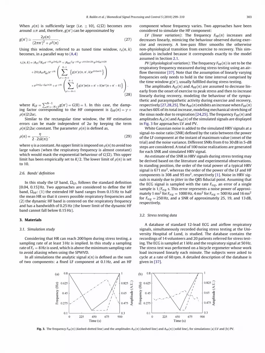
ampling rate of at least 3 Hz is implied. In this study a samplingate of Fs = 8 Hz is used, which is above the minimum sampling rateo avoid aliasing when using the SPWVD.

In all simulations the analytic signal x(n) is defined as the sumf two components: a fixed LF component at 0.1 Hz, and an HF

Fig. 3. The frequency FHF(n) (dashed-dotted line) and the amplitudes ALF(n)

ing and Control 5 (2010) 299–310 303

component whose frequency varies. Two approaches have beenconsidered to simulate the HF component:

LV (linear variation): The frequency FHF(n) increases anddecreases linearly, mimicing the behaviour observed during exer-cise and recovery. A low-pass filter smooths the otherwisenon-physiological transition from exercise to recovery. This sim-ulation is included because it corresponds exactly to the modelassumed in Section 2.1.

PV (physiological variation): The frequency FHF(n) is set to be therespiratory frequency measured during stress testing using an air-flow thermistor [37]. Note that the assumption of linearly varyingfrequencies only needs to hold in the time interval comprised bythe time window g(n′), usually fulfilled during stress testing.

The amplitudes ALF(n) and AHF(n) are assumed to decrease lin-early from the onset of exercise to peak stress and then to increaselinearly during recovery, modeling the behaviour of the sympa-thetic and parasympathetic activity during exercise and recovery,respectively [27,28,25]. The AHF(n) exhibits an increase when FHF(n)reaches 60% of its total increase, modeling mechanical stretching ofthe sinus node due to respiration [24,25]. The frequency FHF(n) andamplitudes ALF(n) and AHF(n) of the simulated signals are displayedin Fig. 3 for approaches LV and PV.

White Gaussian noise is added to the simulated HRV signals at asignal-to-noise ratio (SNR) defined by the ratio between the powerof the LF component at the instant of maximum value (onset of thetrial) and the noise variance. Different SNRs from 0 to 30 dB in 5-dBsteps are considered. A total of 100 noise realizations are generatedfor each SNR and simulated HRV signal.

An estimate of the SNR in HRV signals during stress testing maybe derived based on the literature and experimental observations.In standing position, the order of the total power of a typical HRVsignal is 671 ms2, whereas the order of the power of the LF and HFcomponents is 308 and 95 ms2, respectively [1]. Noise in HRV sig-nals is mainly due to jitter in the QRS fiducial point. Assuming thatthe ECG signal is sampled with the rate Fecg , an error of a singlesample is 1/Fecg s. This error represents a noise power of approxi-mately 1 ms2 for Fecg = 1000 Hz, 4 ms2 for Fecg = 500 Hz and 16 ms2

for Fecg = 250 Hz, and a SNR of approximately 25, 19, and 13 dB,respectively.

3.2. Stress testing data

A database of standard 12-lead ECG and airflow respiratorysignals, simultaneously recorded during stress testing at the Uni-versity Hospital of Lund, is studied. The database contains therecordings of 14 volunteers and 20 patients referred for stress test-

ing. The ECG is sampled at 1 kHz and the respiratory signal at 50 Hz.The stress test was performed on a bicycle ergometer whose workload increased linearly each minute. The subjects were asked tocycle at a rate of 60 rpm. A detailed description of the database isgiven in [37].

(dashed line) and AHF(n) (solid line), for simulations (a) LV and (b) PV.

304 R. Bailón et al. / Biomedical Signal Processing and Control 5 (2010) 299–310

Table 1Parameter values.

Parameter 2M 2K − 1 � 2N − 1 � � u2˛

Value 1024 1023 1/128 81 a 255 b 0.0133 0.0084 6.6667 × 10−6

−1 ample

ibarHwfpHpai

sFqt

cea

FP

Units Samples Samples Samples S

a Length of the rectangular time window.b Length of the tuned time window.

First, QRS detection is performed using Aristotle[38]. Then, thenstantaneous HR signal, dHR(n), is computed following a methodased on the integral pulse frequency modulation model, whichccounts for the presence of ectopic beats [39]. The HR signal isesampled at a sampling rate of Fs = 8 Hz. A time-varying meanR signal dHRM(n) is obtained by low-pass filtering the HR signalith a cut-off frequency of 0.03 Hz. The HRV signal dHRV(n) results

rom dHRV(n) = dHR(n) − dHRM(n). The HRV signal dHRV(n) is low-ass filtered with a cut-off frequency of 0.9 Hz since a spurious 1-z component is sometimes observed [26], being synchronous toedalling at 60 rpm but most likely unrelated to parasympatheticctivity [34,40]. The respiratory frequency does not exceed 0.9 Hzn any of the recordings of the database.

The respiratory frequency is estimated from the airflow signal bypectral analysis [37]. The estimated respiratory frequency series

ˆr(n) is resampled at 8 Hz and low-pass filtered with a cut-off fre-uency of 0.01 Hz to avoid non-physiological abrupt variations dueo estimation errors.

Four subjects were excluded from the study because dHR(n)ontained too many artifacts or ectopic beats to obtain a reliablestimation of the HRV signal based on a criterion adapted from [39],nd one subject was excluded because of unattached electrodes.

ig. 4. Mean ± SD of the estimation error of AHF(n) in relative units (%) achieved by me= 8, 12, 16 (white, gray, dark gray) and SNR of 5, 15, and 25 dB. Numerical values are gi

s Samples Hz/s

4. Results

4.1. Simulation study

The following methods are applied to the simulated HRV signals:UCR: U nconstrained LS estimation using a C onstant length R

ectangular time window.CVR: C onstrained LS estimation using a (2N(n) − 1)-V arying

length R ectangular time window.CVT: C onstrained LS estimation using a T uned time window

with V arying factor (n).Parameter values used are given in Table 1.The estimated number of damped sinusoids, I(n), is 2 during the

majority of the time for methods UCR, CVR and CVT and all modelorders considered, even for a SNR as low as 5 dB, due to the SVDtruncation of Rx(n).

The mean and standard deviation (SD) of the estimation errors(in absolute value) are calculated for ALF(n), FLF(n), AHF(n), and

FHF(n), averaging 100 realizations for each SNR.

For all methods, FLF(n) and FHF(n) were associated with errorslower than 0.002 ± 0.004 Hz (mean ± SD) even for an SNR as low as15 dB and a model order as low as P = 8. The inclusion of informa-

thods UCR, CVR and CVT in simulations (a) LV and (b) PV. Results are shown forven for P = 8, 12, 16.

R. Bailón et al. / Biomedical Signal Process

Table 2Results of the t-test applied to estimates AHF(n) obtained by methods UCR, CVR andCVT. T% and p stand for the percentage of time during which p <0.05 and the meanp-value during that time, respectively, for simulation PV.

P T% (p)

UCR–CVR UCR–CVT CVR–CVT

(a) 25 dB8 95 (6 × 10−4) 96 (5 × 10−4) 97 (2 × 10−4)12 93 (6 × 10−4) 97 (3 × 10−4) 97 (3 × 10−4)16 92 (7 × 10−4) 97 (3 × 10−4) 98 (2 × 10−4)

(b) 15 dB8 85 (2 × 10−3) 83 (2 × 10−3) 94 (7 × 10−4)12 83 (2 × 10−3) 86 (1 × 10−3) 94 (7 × 10−4)16 80 (3 × 10−3) 89 (1 × 10−3) 94 (7 × 10−4)

(c) 5 dB

tt

roaa2d

avtfs

CatepfbdaSm

Fa

8 66 (5 × 10−3) 56 (6 × 10−3) 80 (3 × 10−3)12 72 (5 × 10−3) 48 (7 × 10−3) 79 (3 × 10−3)16 64 (5 × 10−3) 41 (9 × 10−3) 79 (3 × 10−3)

ion on respiratory frequency mainly affects AHF(n). Fig. 4 presentshe estimation error of AHF(n) for the simulations LV and PV.

For simulation LV, Fig. 4(a) shows that the inclusion of respi-atory information leads to a reduction of the estimation errorf AHF(n) at low SNRs, i.e., 15 and 5 dB, the smallest errors beingchieved when the tuned window is used. A reduction in SD ischieved at the expense of a slight increase in mean for SNR of5 dB. It is obvious from Fig. 4(a) that the estimation error does notepend on P when respiratory information is included.

For simulation PV, Fig. 4(b) shows that respiratory informationgain leads to a reduction of the estimation error of AHF(n) for allalues of SNR and P. It is noted that the estimation errors are smallerhan those obtained in simulation LV. It is also noted that the dif-erences in estimation error between simulations LV and PV are themallest for CVT.

In order to test if estimates AHF(n) obtained by methods UCR,VR and CVT are statistically significant, a two-sample t-test ispplied to each of the 3 possible pairwise comparisons for eachime instant n. The percentage of the total time, T%, during whichstimates AHF(n), are statistically significant (p-value<0.05) is dis-layed in Table 2, as well as the mean p-value during that time, p,or simulation PV. It can be observed that estimates AHF(n) obtained

y UCR, CVR and CVT are significantly different from each otheruring most of the time and with a small mean p-value (T% ≥ 92%nd p ≤ 7 × 10−4 for all model orders) for a SNR of 25 dB. For lowerNRs, lower values of T% as well as higher values of p are observed,ainly due to the increase in the SD of the estimates. However esti-

ig. 5. (a) Simulated HRV signal R{x(n)}, (b) FLF(n) (dashed line) and FHF(n) (dotted line), (SNR of 15 dB. See Fig. 3 for original trends.

ing and Control 5 (2010) 299–310 305

mates AHF(n) obtained by CVR and CVT are significantly differentduring at least 80% of the total time (p ≤ 3 × 10−3) even for a SNR of5 dB.

The estimation error of ALF(n) is similar to that of AHF(n) whenrespiratory information is not included in the estimation of AHF(n)(results not displayed), always that the model order is high enough.

Fig. 5 displays the simulated signal and the correspondingestimates FLF(n), FHF(n), ALF(n), and AHF(n), obtained by CVT forsimulation PV.

4.2. Stress testing data

The methods UCR and CVT are applied to the stress testing HRVsignals, using parameter values identical to those in the simula-tions, see Table 1. The standard HF band and the extended HF bandare used with UCR because no respiratory information is included,whereas the dynamic HF band is used with CVT.

The signals dHR(n) and dHRV(n) are displayed in Fig. 6(a) and(b), respectively, for a volunteer of the present database. The non-stationary nature of dHR(n) can be appreciated not only in its trend,which increases approximately linearly from onset to peak stressand decreases abruptly during recovery, but also in dHRV(n) with itsprogressive diminution of HRV from onset to peak stress and thenits abrupt increase during recovery. The corresponding Px(n, m) iscomputed using UCR and CVT and displayed in Fig. 6(c) and (d),respectively.

Fig. 7 displays the corresponding FLF(n), PLF(n), FHF(n), and PHF(n)obtained with UCR, using either the standard or the extended HFband, and CVT, using the dynamic HF band.

For stress testing data, a lower value of P is preferred than forsimulated data so as to obtain smoother estimates when the LFand HF bands do not exhibit a dominant peak. Due to the SVDtruncation of Rx(n), the estimated number of damped sinusoidsI(n) equals 1 approximately 80% of the time, and 2 the 20% left.However, if a less restrictive SVD truncation is considered, the I(n)increases significantly even for low model orders, making it diffi-cult the identification of the LF and HF components. Note that whenthe respiratory frequency exceeds 0.4 Hz from about 400 to 700 s,the standard HF band leads to misestimation of the HF component(see Fig. 7(a)). This problem is avoided when either UCR, using theextended HF band (Fig. 7(b)), or CVT, using the dynamic HF band

(Fig. 7(c)), is employed. In that case CVT leads to smoother esti-mates PHF(n) than does UCR. In order to quantify the smoothnessof the estimate PHF(n), the SD around a mean trend, obtained bylow-pass filtering of PHF(n) with a cut-off frequency of 0.01 Hz, iscomputed. This value is averaged among the 30 recordings of the

c) ALF(n), and (d) AHF(n), estimated using method CVT, for a model order P = 16 and

306 R. Bailón et al. / Biomedical Signal Processing and Control 5 (2010) 299–310

F Px(n, m3

df

TwdbasftPer

otit(

Fa

ig. 6. (a) Instantaneous HR signal dHR(n), (b) HRV signal dHRV(n), and the SPWVD.2.

atabase, yielding a mean ± SD of 0.74 × 10−3 ± 1.03 × 10−3 s−2

or UCR and of 0.12 × 10−3 ± 0.18 × 10−3 s−2 for CVT.Fig. 7(b) shows trends which are similar to those in Fig. 7(c).

he FLF(n) varies slightly around 0.08 Hz during the whole test,hile the FHF(n) increases from onset to peak stress and decreasesuring recovery. The trend PLF(n) shows a rapid decrease at theeginning of exercise, reaching a plateau which is maintained untilpproximately 100 s before the peak stress, when PLF(n) is almostuppressed. During recovery, the initial abrupt increase in PLF(n) isollowed by a progressive return to the value at the beginning ofhe exercise. The PHF(n) is decreased from onset to peak stress, butˆHF(n) is not suppressed around the peak stress. During the recov-ry there is an increase in PHF(n), less steep than in PLF(n), beforeeturning to its value at the beginning of the exercise.

To test the hypothesis that the differences between PHF(n)

btained by UCR (with the extended HF band) and CVT are sta-istically significant, a one-sample t-test is applied for each timenstant n to the 14 volunteers of the database. The percentage ofhe total time during which differences are statistically significantp-value<0.05) is T% = 25%, and the mean p-value during that time is

ig. 7. The frequency trends FLF(n) and FHF(n) (top), PLF(n) (middle), and PHF(n) (bottom)nd dynamic HF band. The model order is P = 8. Stress peak is marked with a dashed line

) using methods (c) UCR and (d) CVT for a volunteer from the database of Section

p = 0.01. Since statistical significance is highly affected by the num-ber of realizations (14 in this case), and to make statistical resultscomparable to those in the simulation study (100 realizations), thet-test is also applied to a total of 98 realizations, obtained by repli-cating results from the 14 volunteers, yielding statistical values ofT% = 66% and p = 0.005.

Fig. 8 displays the mean ± SD of the parameters FLF(n), PLF(n),FHF(n), and PHF(n), estimated using CVT and evaluated at differ-ent time instants during the stress test and averaged for the 14volunteers. The time instants considered are: the first minute ofexercise (n1), 3 min before the peak stress (n2), 1 min before thepeak stress (n3), 1 min after the peak stress (n4) and 3 min afterthe peak stress (n5). At each time instant, the parameter value isobtained by averaging the trend in a 1-s window.

Fig. 8 demonstrates that the over-all characteristics of the HRV

trends of the 14 volunteers resemble those observed for the vol-unteer of Fig. 7. However, a large variability among subjects isobserved in PLF(n) and PHF(n), especially at n5, which may reflectthe large intersubject variability that exists in HRV signals [4],especially during the recovery. To test the hypothesis that the dif-

, using (a) UCR and standard HF band, (b) UCR and extended HF band, and (c) CVT.

R. Bailón et al. / Biomedical Signal Processing and Control 5 (2010) 299–310 307

Fig. 8. Mean ± SD among the 14 volunteers of the parameters (a) FLF(n), (b) PLF(n), (c) FHF(nn2 (3 min before the peak stress), n3 (1 min before the peak stress), n4 (1 min after the pea

Table 3The p-value obtained by the Wilcoxon signed rank test. The time instants are n1 (thefirst minute of exercise), n2 (3 min before the peak stress), n3 (1 min before the peakstress), n4 (1 min after the peak stress) and n5 (3 min after the peak stress).

FHF(n) n2 n3 n4 n5

n1 0.0023 0.0017 0.0012 0.3910n2 – 0.1938 0.1937 0.0052n3 – – 0.0203 0.0052n4 – – – 0.0040

PLF(n) n2 n3 n4 n5

n1 0.0007 0.0024 0.1189 0.4548n2 – 0.1016 0.0007 0.1763n3 – – 0.0005 0.0137n4 – – – 0.0171

PHF(n) n2 n3 n4 n5

n1 0.0001 0.0001 * 0.0580n2 – 0.9515 0.0012 0.0012n3 – – 0.0031 0.0009

fmbp(mfs

5

5

iwitqnttraio

tvit

It is assumed that the HRV signal during stress testing can be

n4 – – – 0.1937

* p > 0.05.

erences of HRV parameters between two time instants has zeroedian, a Wilcoxon signed rank test is applied to the 10 possi-

le pair-wise comparisons of the 5 different time instants for eacharameter (FLF(n), PLF(n), FHF(n), and PHF(n)). The significance levelp-value) at which the null hypothesis of differences with zero

edian can be rejected is displayed in Tab. 3. Results are not shownor FLF(n) since only the comparison FLF(n3) − FLF(n5) obtained aignificant p-value of 0.0137.

. Discussion

.1. Methodological aspects

In this paper the analysis of non-stationary HRV signals dur-ng stress testing is addressed by parametric decomposition of the

indowed and filtered instantaneous ACF on which the SPWVDs based. The advantage of using a parametric decomposition ofhe instantaneous ACF is that information such as respiratory fre-uency can be included in the model. Respiratory information isot necessarily obtained from a simultaneously recorded respira-ion signal but can also be derived from the ECG signal using, e.g.,he method described in [37], which has been shown to provideeliable respiratory frequency estimates during stress testing (withmean error of 0.022 ± 0.016 Hz in a database of 29 subjects). The

nclusion of respiratory information mainly affects the estimationf the amplitude of the HF component.

The inclusion of respiratory information in the definition of theime window makes estimation errors independent of the rate ofariation of the respiratory frequency. This leads to shorter averag-ng for higher rates of variation, which results in less reduction ofhe cross terms and the noise. As a consequence, in benefit of the

), and (d) PHF(n), estimated by CVT and evaluated at n1 (the first minute of exercise),k stress), and n5 (3 min after the peak stress).

tracking of faster variations, estimation errors may be larger in thepresence of high levels of noise.

The inclusion of respiratory frequency information as a con-straint in the LS estimation leads to a reduction in both the meanand SD of the estimation error of the HF amplitude. This reductiondepends on the time window used and on the SNR, and turns outto be larger when the tuned window is used or when lower SNRsare analyzed. For example, when the frequency of the HF compo-nent follows a real respiratory frequency, a reduction in mean from3.5% to 2.4%, and in SD from 3.0% to 1.7%, is achieved using thetuned window for a SNR of 15 dB. For a real respiratory frequencysimilar results were obtained for both the tuned and the rectangu-lar window. Estimation errors for a linearly varying HF frequencyare, in general, larger than for a real respiratory frequency, and thereduction in the estimation error using a tuned window instead ofa rectangular window is more evident for a linearly varying HF fre-quency than for a real respiratory frequency. These results may bedue to the fact that the rate of variation is slower for the simulationwith a real respiratory frequency. Estimation errors obtained withthe tuned window are similar for both situations, thus pointing toanother advantage of the tuned window. Results from the stresstesting database show that the inclusion of respiratory informa-tion as a constraint in the LS estimation (using the tuned window)leads to smoother trends of the power of the HF component.

The inclusion of respiratory information in the HF band defini-tion accounts for the fact that respiratory frequency is not restrictedto the standard HF band during stress testing. In Fig. 7, it is shownthat the use of the standard HF band would have yielded a misesti-mation of the HF component, which incorrectly can be interpretedas a suppression of the parasympathetic activity. If respiratoryinformation is not available, this can be avoided using an extendedHF band [0.15, dHRM(n)/2] Hz [9,13]. In that case, care should betaken since other HF components unrelated to the parasympatheticactivity can be merged with the respiration-related HF component(e.g. a component synchronous with the pedalling frequency [26]).

A proper selection of the time and frequency windows of theSPWVD should guarantee the reduction of the interference terms,and the decomposition of the windowed and filtered ACF as a sumof complex damped sinusoids. In this paper, an exponential win-dow is used for frequency smoothing, and either a rectangular ora tuned window for time smoothing; other types of windows havebeen proposed for the analysis of HRV [15,16]. A prospective studyon a larger database would be needed to obtain the most suitablevalues for the parameters. An alternative to reduce the interferenceterms could have been filtering the signal in the LF and HF bandsand applying the proposed method in each band to estimate the LFand HF components separately. However, this would have requiredproper cut-off frequencies selection, with a particular risk when theLF and HF bands are time-varying.

modeled as a sum of two sinusoids for which the frequency of theHF component varies linearly over time. While the assumption ofa linearly varying HF frequency may seem drastic, it only needs tohold in the interval extended by the time window. The frequency

3 rocess

oiitdbtafipscftpi[asev

tmltitsoawhntteoaicfctaspmmewperabamapp

5

a

08 R. Bailón et al. / Biomedical Signal P

f the LF component can also vary during stress testing, however,ts variation is much smaller than that of the HF component andt is therefore assumed to be constant. Even if the amplitudes ofhe LF and HF components can vary during stress testing, in theerivation of the windowed and filtered ACF they are assumed toe constant in the interval extended by the time window, givenhat their variations are assumed to be slow compared with the LFnd HF frequencies so that the “quasi-stationary” condition is ful-lled [31]. Although the simulated signals generated to assess theerformance of the method deviate from the assumed model in theense that they include time-varying amplitudes for the LF and HFomponents and an HF frequency which follows a real respiratoryrequency evolution during stress testing (no linearly varying as inhe model), the simulated HRV signals are not able to represent theseudo-stochastic nature of HRV signals, nor the nonlinear dynam-

cs which may be involved in the regulation of the ANS on the heart4]. An improved generator of synthetic HRV signals is needed tossess the performance of the method in real-life stress testing HRVignals [19]. Even with such synthetic HRV signals available, thevaluation on real stress testing HRV signals will still be of limitedalue as no reference “true” signal exists.

Assuming the same model for the HRV signal during stressesting, alternative approaches such as maximum likelihood esti-

ation or noise subspace methods can be considered. The mainimitation of these methods is that they assume the stationarity ofhe signal, in contrast to TF methods, so they need to be appliedn short time windows in which the signal can be considered sta-ionary. Different methods for the analysis of non-stationary HRVignals have been proposed in the literature. In [8] an extensiveverview of methods for the continuous quantification of the LFnd HF components in non-stationary HRV signals is presented,here advantages and limitations of the different approaches areighlighted. A comparison between the methods is unfortunatelyot straightforward, since different approaches to TF representa-ion and HRV parameter estimation can be taken. For example,ime-varying autoregressive analysis comes with the selection ofstimation method for the time-varying coefficients and modelrder. Although spectral decomposition can be used for frequencynd power estimation of the spectral components, a criterions needed for the identification and tracking of the LF and HFomponents. Time-varying autoregressive analysis offers accuraterequency estimation but less accurate power estimation, espe-ially when rapid changes occur [16,19] and when poles are close tohe unit circle [8] as may be the case during stress testing. Waveletnalysis has also been used for the analysis of non-stationary HRVignals, however, as pointed out in [8], power computation may beroblematic when scales and bands do not properly match or whenore than one spectral component is present at a given scale, whichay be the case during stress testing when respiratory frequency

xhibits a large variation or when the component synchronousith the pedaling frequency is present [26]. The instantaneousower of the LF and HF components could have been alternativelystimated by integration of the SPWVD in the LF and HF bands,espectively. However, these estimates are affected by the timend frequency smoothing windows, whose effect is diminishedy the parametric decomposition described in this paper, whichlso allows the inclusion of respiratory frequency information. Theethod described in this paper has been selected based on the

ppropriate TF resolution of the SPWVD and, especially, on theossibility of including respiration information, as proposed in thisaper.

.2. Physiological aspects

From analysis of the stress testing database (see Figs. 7 and 8)progressive reduction of the LF power can be observed as the

ing and Control 5 (2010) 299–310

stress level increases, when the sympathetic activity is thoughtto increase also, becoming nearly abolished when peak stress isreached [27,28,41]. This would suggest either that the LF poweris not a valid marker of the sympathetic activity, at least duringexercise [42,43,29,4], or that some kind of saturation prevents theLF power to increase at the rate of the sympathetic stimulation.In the recovery phase there is an abrupt increase in the LF powerwhich may be due to sympathetic activity or a rapid decrease inHR, which leaks in the LF band. The HF power is also reduced fromthe beginning of the exercise, which might reflect withdrawal ofparasympathetic activity [27,28,4], which would allow the HR toincrease and satisfy the increasing metabolic demand. While someconsider HF power as a valid marker of parasympathetic activityduring exercise [29], it is not always suppressed near peak stresswhen the parasympathetic activity is inhibited. This suggests theexistence of a non-neural mechanism which causes mechanicalstretching of the sinus node due to respiration [24,25]. However, inthe recordings analyzed in Figs. 7 and 8, this effect is not so evident.The reason may be that the recordings come from volunteers, whoperform a submaximal exercise stress test (up to a rate of perceivedexertion (RPE) of 15 out of 20 on the Borg scale) [37]. Finally, the HFpower increases in the recovery phase when the parasympatheticactivity is supposed to be reestablished. In Figs. 7 and 8, it can beappreciated that the values of the LF and HF powers are differentat the beginning and at the end of the stress testing. This might bedue to the different body position at the beginning (sitting, sympa-thetic dominance) and at the end of the test (lying, parasympatheticdominance).

A hypothesis of this work is that the frequency of the HF compo-nent coincides with respiratory frequency. However, a reduction inthe spectral coherence between the HRV and the respiration signalin the HF band in the last part of the exercise has been reported[44]. The coherence information may be also included in the HRVparameter estimation in a further study.

Finally, an important point to be discussed in the framework ofthis study is the use of the HRV analysis as a tool to assess changesin ANS during stress testing. It is generally accepted that HRV can beconsidered as a noninvasive measure of the ANS activity in station-ary conditions [1]. The underlying assumption is that mean heartrate and respiratory frequency and air flow volume are stationary.During stress testing both the respiratory frequency and the air flowvolume vary, yielding variations in the HF power which may beunrelated to the parasympathetic activity. Moreover, during stresstesting the time-varying mean heart rate may obscure the inter-pretation of the evolution of the sympathetic and parasympatheticactivity based on the LF and HF power estimates.

6. Conclusions

In this paper a novel method for the time-varying analysis ofHRV during exercise stress testing including information on respi-ratory frequency has been presented. Respiratory information hasbeen included in different parts of the analysis: in the definition ofa dynamic HF band centered on the respiratory frequency, in thedesign of the time window based on the rate of variation of therespiratory frequency, and in the parametric decomposition as aconstraint. Results from both the simulation study and the stresstesting database show that the inclusion of respiratory informationprovides more robust estimates of the HF component in terms ofmean errors and SD. The application of this technique to the stress

testing database evidences a significant decrease in the power ofboth the LF and HF components in the vicinity of peak stress withrespect to both the beginning of the exercise and the recovery. Thistechnique can be employed to assess the, still debated, relation-ships between ANS control and exercise stress.

rocess

A

nbpC

A

re

w

c

E

F

w

r

A

Lb

[

[

[

[

[

[

[

[

[

[

R. Bailón et al. / Biomedical Signal P

cknowledgements

This study was supported by Ministerio de Ciencia y Tec-ología, Spain, under Project TEC2007-68076-C02-02/TCM, in party the Diputación General de Aragón (DGA), Spain, through Gru-os Consolidados GTC ref:T30, by ISCIII, Spain, through CIBERB06/01/0062, and by CAI, Spain, through Programa Europa XXI.

ppendix A.

Derivation of the windowed and filtered ACF in (3) when theectangular window g(n′) in (5) is used for time smoothing and thexponential window |h(k)|2 in (6) is used for frequency smoothing:

rx(n, k) = |h(k)|2[

N−1∑n′=−N+1

g(n′)x(n + n′ + k)x∗(n + n′ + k)

]

= e−� |k| 12N − 1

N−1∑n′=−N+1

(|ALF|2ej2�fLF2k +|AHF|2ej2�(2˛(n+n′)+ˇ)2k

+ 2R{ALFA∗HF}c(n, n′, k) ej2�(fLF+2˛(n+n′)+ˇ)k

+w(n + n′ + k)w∗(n + n′ − k)) ,(A.1)

here

(n, n′, k) = cos[2�{˛[(n + n′)2 + k2] + (ˇ − fLF)(n + n′)}]. (A.2)

q. (A.1) becomes

rx(n, k) = |ALF|2e−� |k|ej2�fLF2k + 12N − 1

|AHF|2e−� |k|

(N−1∑

n′=−N+1

ej2�2˛n′2k

)ej2�(2˛n+ˇ)2k

+ 12N − 1

2R{ALFA∗HF}e−� |k|

(N−1∑

n′=−N+1

c(n, n′, k)ej2�2˛n′k

)ej2�(fLF+2˛n+ˇ)k

+ 12N − 1

e−� |k|

(N−1∑

n′=−N+1

w(n + n′ + k)w∗(n + n′ − k)

).

(A.3)

inally

rx(n, k) = |ALF|2e−� |k|ej2�fLF2k + 12N − 1

|AHF|2e−� |k| sin(2�2˛(2N − 1)k)sin(2�2˛k)

ej2�fHF(n)2k

+ 12N − 1

2R{ALFA∗HF}e−� |k|

(N−1∑

n′=−N+1

c(n, n′, k)ej2�2˛n′k

)

× ej2�(fLF+fHF(n))k

+ rw(n, k),(A.4)

here

w(n, k) = 12N − 1

e−� |k|

(N−1∑

n′=−N+1

w(n + n′ + k)w∗(n + n′ − k)

).

(A.5)

ppendix B.

Derivation of the constrained LS estimator of (18) using

agrange multipliers. Taking the derivative of (18) with respect to∗(n) and setting it equal to zero yields

∂Jc,n

∂b∗(n)= RH

x (n)rx(n) + RHx (n)Rx(n)b(n) + 1

2�z∗

HF(n) = 0. (B.1)[

ing and Control 5 (2010) 299–310 309

The constrained LS estimator of b(n) is given by

bc(n) = b(n) − 12

�(

RHx (n)Rx(n)

)−1z∗

HF(n). (B.2)

Substituting (B.2) in (17), the Lagrange multiplier � can be found,

�=2[bT(n)zHF(n)+1]

(zH

HF(n)[(

RHx (n)Rx(n)

)−1]T

zHF(n)

)−1

, (B.3)

and finally,

bc(n) = b(n) −(

bT(n)zHF(n) + 1

)(zH

HF(n)

[(RH

x (n)Rx(n))−1]T

zHF(n)

)−1

×(

RHx (n)Rx(n)

)−1z∗

HF(n). (B.4)

References

[1] The Task Force of ESC and NASPE, Heart rate variability. Standards of mea-surement, physiological interpretation, and clinical use, Eur. Heart J. 17 (1996)354–381.

[2] A. Bianchi, L. Mainardi, E. Petrucci, M. Signorini, M. Mainardi, S. Cerutti, Time-variant power spectrum analysis for the detection of transient episodes in HRVsignal, IEEE Trans. Biomed. Eng. 40 (2) (1993) 136–144.

[3] F. Lombardi, A. Malliani, M. Pagani, S. Cerutti, Heart rate variability and itssympatho-vagal modulation, Cardiovasc. Res. 32 (1996) 208–216.

[4] A. Aubert, B. Seps, F. Beckers, Heart rate variability in athletes, Sports Med. 33(12) (2003) 889–919.

[5] R. Bailón, J. Mateo, S. Olmos, P. Serrano, J. García, A. del Río, I. Ferreira, P. Laguna,Coronary artery disease diagnosis based on exercise electrocardiogram indexesfrom repolarisation, depolarisation and heart rate variability, Med. Biol. Eng. &Comput. 41 (2003) 561–571.

[6] R. Hainsworth, The control and physiological importance of heart rate, in: M.Malik, A. Camm (Eds.), Heart Rate Variability, Futura Publishing Company, Inc,New York, 1995, pp. 3–19.

[7] F. Cottin, Y. Papelier, Regulation of cardiovascular system during dynamic exer-cise: integrative approach, Crit. Rev. Physical Rehab. Med. 14 (1) (2002) 53–81.

[8] L. Mainardi, On the quantification of heart rate variability spectral parametersusing time–frequency and time-varying methods, Phil. Trans. R. Soc. A 367(2009) 255–275.

[9] L. Keselbrener, S. Akselrod, Selective discrete Fourier transform algorithm fortime–frequency analysis: method and application on simulated and cardiovas-cular signals, IEEE Trans. Biomed. Eng. 43 (8) (1996) 789–802.

10] O. Meste, B. Khaddoumi, G. Blain, S. Bermon, Time-varying analysis methodsand models for the respiratory and cardiac system coupling in graded exercise,IEEE Trans. Biomed. Eng. 52 (11) (2005) 1921–1930.

11] K. Martinmäki, H. Rusko, S. Saalasti, J. Kettunen, Ability of short-time Fouriertransform method to detect transient changes in vagal effects on hearts: apharmacological blocking study, Am. J. Physiol. Heart Circ. Physiol. 290 (2006)H2582–H2589.

12] D. Verlinde, F. Beckers, D. Ramaekers, A.E. Aubert, Wavelet decomposition anal-ysis of heart rate variability in aerobic athletes, Auton. Neurosci. 90 (1–2) (2001)138–141.

13] E. Toledo, O. Gurevitz, H. Hod, M. Eldar, S. Akselrod, Wavelet analysis of instan-taneous heart rate: a study of autonomic control during thrombolysis, Am. J.Physiol. Regul. Integr. Comp. Physiol. 284 (2003) R1079–R1091.

14] Y. Goren, L. Davrath, I. Pinhas, E. Toledo, S. Akselrod, Individual time-dependentspectral boundaries for improved accuracy in time–frequency analysis of heartrate variability, IEEE Trans. Biomed. Eng. 53 (1) (2006) 35–42.

15] P. Novak, V. Novak, Time/frequency mapping of the heart rate, blood pressureand respiratory signals, Med. Biol. Eng. & Comput. 31 (2) (1993) 103–110.

16] S. Pola, A. Macerata, M. Emdin, C. Marchesi, Estimation of the power spectraldensity in non-stationary cardiovascular time series: assessing the role of thetime–frequency representations (TFR), IEEE Trans. Biomed. Eng. 43 (1) (1996)46–59.

17] L. Mainardi, N. Montano, S. Cerutti, Automatic decomposition of Wigner distri-bution and its application to heart rate variability, Methods Inf. Med. 43 (2004)17–21.

18] A. Bianchi, L. Mainardi, C. Meloni, S. Chierchia, S. Cerutti, Continuous monitoringof the sympatho-vagal balance through spectral analysis. Recursive autoregres-sive techniques for tracking transient events in heart rate signals, IEEE Eng. Med.Biol. Mag. 16 (5) (1997) 64–73.

19] M. Orini, R. Bailón, P. Laguna, L. Mainardi, Modeling and estimation of

time-varying heart rate variability during stress test by parametric and nonparametric analysis, in: Proceedings of Computers in Cardiology, Vol. 34,http://cinc.mit.edu, 2007, pp. 29–32.

20] S. Akselrod, D. Gordon, F. Ubel, D. Shannon, A. Barger, R. Cohen, Power spec-trum analysis of heart rate fluctuations: a quantitative probe of beat-to-beatcardiovascular control, Science 213 (1981) 220–222.

3 rocess

[

[

[

[

[

[

[

[

[

[

[

[

[

[

[

[

[

[

[

[

[

[

[quency on heart rate and blood pressure variability during dynamic exercise,

10 R. Bailón et al. / Biomedical Signal P

21] B. Pomeranz, R. Macaulay, M. Caudill, Assessment of autonomic function inhumans by heart rate spectral analysis, Am. J. Physiol. 248 (1985) H151–H153.

22] P. Grossman, K. Wientjes, Respiratory sinus arrhythmia and parasympatheticcardiac control: some basic issues concerning quantification, applications andimplications, in: P. Grossman, K. Jansenn, D. Waitl (Eds.), Cardiorespiratory andcardiosomatic psycophysiology, Plenum Press, NY, 1986, pp. 117–138.

23] M. Pagani, D. Lucini, O. Rimoldi, R. Furlan, S. Piazza, L. Biancardi, Effects of phys-ical and mental exercise on heart rate variability, in: M. Malik, A. Camm (Eds.),Heart Rate Variability, Futura Publishing Company, Inc, New York, 1995, pp.245–266.

24] L. Bernardi, F. Salvucci, R. Suardi, P. Solda, A. Calciati, S. Perlini, C. Falcone, L.Ricciardi, Evidence for an intrinsic mechanism regulating heart rate variabilityin the transplanted and the intact heart during submaximal dynamic exercise?Cardiovasc. Res. 24 (12) (1990) 969–981.

25] G. Blain, O. Meste, S. Bermon, Influences of breathing patterns on respiratorysinus arrhythmia in humans during exercise, Am. J. Physiol. Heart Circ. Physiol.288 (2005) H887–H895.

26] R. Bailón, P. Laguna, L. Mainardi, L. Sörnmo, Analysis of heart rate variabilityusing time-varying frequency bands based on respiratory frequency, in: Proc.29th Int. Conf. IEEE Eng. Med. Biol. Soc., IEEE-EMBS Society, Lyon, 2007, pp.6674–6677.

27] R. Perini, C. Orizio, G. Baselli, The influence of exercise intensity on the powerspectrum of heart rate variability, Eur. J. Appl. Physiol. 61 (1990) 143–148.

28] Y. Yamamoto, R. Hughson, J. Peterson, Autonomic control of heart rate duringexercise studied by heart rate variability spectral analysis, J. Appl. Physiol. 71(3) (1991) 1136–1142.

29] J. Warren, R. Jaffe, C. Wraa, C. Stebbins, Effect of autonomic blockade on powerspectrum of heart rate variability during exercise, Am. J. Physiol. 273 (1997)R495–R502.

30] O. Anosov, A. Patzak, Y. Kononovich, P. Persson, High-frequency oscillations ofthe heart rate during ramp load reflect the human anaerobic threshold, Eur. J.

Appl. Physiol. 83 (4–5) (2000) 388–394.

31] W. Martin, P. Flandrin, Wigner-Ville spectral analysis of nonstationary pro-cesses, IEEE Trans. Acoust. Speech Signal Proc. 33 (6) (1985) 1461–1470.

32] T. Claasen, W. Mecklenbräuker, The Wigner distribution - A tool fortime–frequency signal analysis. Part II: discrete-time signals, Philips J. Res. 35(1980) 276–300.

[

ing and Control 5 (2010) 299–310

33] P. Flandrin, W. Martin, Pseudo-Wigner estimators for the analysis of non-stationary processes, in: Proc. IEEE Acoust. Speech Signal Proc. Spectrum Est.Workshop II, 1983, pp. 181–185.

34] O. Meste, G. Blain, S. Bermon, Influence of the pedalling frequency on the heartrate variability, in: Proc. 29th Int. Conf. IEEE Eng. Med. Biol. Soc., IEEE-EMBSSociety, Lyon, 2007, pp. 279–282.

35] R. Kumaresan, D. Tufts, Estimating the parameters of exponentially dampedsinusoids and pole-zero modeling in noise, IEEE Trans. Acoust. Speech SignalProc. 30 (1982) 833–840.

36] R. Kumaresan, On the zeros of the linear prediction-error filter for deterministicsignals, IEEE Trans. Acoust. Speech Signal Proc. 31 (1983) 217–220.

37] R. Bailón, L. Sörnmo, P. Laguna, A robust method for ECG-based estimation ofthe respiratory frequency during stress testing, IEEE Trans. Biomed. Eng. 53 (7)(2006) 1273–1285.

38] G. Moody, R. Mark, Development and evaluation of a 2-lead ECG analysis pro-gram, in: Proc. Comput. Cardiol., vol. 9, IEEE Computer Society Press, 1982, pp.39–44.

39] J. Mateo, P. Laguna, Analysis of heart rate variability in the presence of ectopicbeats using the heart timing signal, IEEE Trans. Biomed. Eng. 50 (2003) 334–343.

40] F. Villa, P. Castiglioni, G. Merati, P. Mazzoleni, M. Di Rienzo, Effects of pedallingon the high frequency components of HRV during exercise, in: Proceedings ofComputers in Cardiology, Vol. 35, http://cinc.mit.edu, 2008, pp. 37–40.

41] R. Perini, N. Fisher, A. Veicsteinas, D.R. Pendergast, Aerobic training and cardio-vascular responses at rest and during exercise in older mean and women, Med.Sci. Sports Exerc 34 (2002) 700–708.

42] Y. Arai, J. Saul, P. Albrecht, L. Hartley, L. Lilly, R. Cohen, W. Colucci, Modulationof cardiac autonomic activity during and immediately after exercise, Am. J.Physiol. Heart Circ. Physiol. 256 (1989) H132–H141.

43] F. Cottin, Y. Papelier, P. Escourrou, Effects of exercise load and breathing fre-

Int. J. Sports Med. 20 (1999) 232–238.44] K. Keissar, L. Davrath, S. Akselrod, Time-frequency wavelet transform

coherence of cardio-respiratory signals during exercise, in: Proceedingsof Computers in Cardiology, Vol. 33, http://cinc.mit.edu, 2006, pp. 733–736.