An unsymmetric 8-node hexahedral solid-shell element with

Received: 27 January 2018 Revised: 10 June 2018 Accepted: 16 August 2018

DOI: 10.1002/nme.5945

R E S E A R C H A R T I C L E

An unsymmetric 8-node hexahedral solid-shell elementwith high distortion tolerance: Linear formulations

Junbin Huang1 Song Cen1,2 Zhi Li1 Chen-Feng Li3

1Department of Engineering Mechanics,School of Aerospace Engineering,Tsinghua University, Beijing, China2AML, School of Aerospace Engineering,Tsinghua University, Beijing, China3College of Engineering, SwanseaUniversity, Swansea, UK

CorrespondenceSong Cen, Department of EngineeringMechanics, School of AerospaceEngineering, Tsinghua University, Beijing100084, China.Email: [email protected]

Funding informationNational Natural Science Foundation ofChina, Grant/Award Number: 11872229;Specialized Research Fund for theDoctoral Program of Higher Education ofChina, Grant/Award Number:20120002110080; Tsinghua UniversityInitiative Scientific Research Program,Grant/Award Number: 2014z09099

Summary

A locking-free unsymmetric 8-node solid-shell element with high distortiontolerance is proposed for general shell analysis, which is equipped with transla-tional degrees of freedom only. The prototype of this new model is a recent solidelement US-ATFH8 developed by combining the unsymmetric finite elementmethod and the analytical solutions in three-dimensional local oblique coor-dinates. By introducing proper shell assumptions and assumed natural strainmodifications for transverse strains, the new solid-shell element US-ATFHS8is successfully formulated. This element is able to give highly accurate predic-tions for shells with different geometric features and loading conditions and isquite insensitive to mesh distortions. In particular, the excellent performanceof US-ATFH8 under membrane load is well inherited, which is an outstandingadvantage over other shell elements.

KEYWORDS

analytical trial functions, finite element methods, mesh distortions, oblique coordinates, solid-shellelements, unsymmetric finite elements

1 INTRODUCTION

Although the finite element method (FEM) is one significant tool and has been widely applied in various engineeringand scientific fields, some key technical challenges remain outstanding. To date, many researchers are still making greatefforts in developing novel high-performance models that can overcome the drawbacks existing in the traditional FEM.1

This paper is mainly about an application of the unsymmetric FEM2 together with the analytical trial function method3 inshell analysis. The unsymmetric FEM can effectively reduce the sensitivity problems to mesh distortions by successfullyeliminating the Jacobian determinant after employing two different sets of interpolation for displacement fields. Theanalytical trial function method makes use of the solutions of governing equations of elasticity as trial functions for finiteelement discretization, which is similar to the Trefftz methods.4 Because of these merits, the resulting models can achievehigh accuracy and naturally avoid many locking problems caused by traditional isoparametric interpolation techniques.5

Recently, the above strategy brought some interesting breakthroughs in low-order finite elements. It is well known thatMacNeal proved an important theorem about 30 years ago,6 which claims that any 4-node, 8-dof (degree of freedom)quadrilateral membrane element must either present trapezoidal locking results for MacNeal's thin-beam problem orfail to guarantee its convergence. This theorem frustrates many scholars who devote themselves to developing low-orderfinite element models. In 2015, Cen et al7 proposed an unsymmetric 4-node, 8-dof membrane element US-ATFQ4 that cancircumvent this issue. A similar scheme has been already generalized to the three-dimensional (3D) case, and an 8-node,

Int J Numer Methods Eng. 2018;116:759–783. wileyonlinelibrary.com/journal/nme © 2018 John Wiley & Sons, Ltd. 759

https://doi.org/10.1002/nme.5945

http://orcid.org/0000-0002-6839-286X

http://orcid.org/0000-0002-8674-4005

http://orcid.org/0000-0003-2495-5816

760 HUANG ET AL.

24-dof hexahedral element US-ATFH8 was successfully formulated.8 Both elements are verified to be not only accurate formost standard benchmark problems but also insensitive to severe mesh distortions. Similar models that can only deal withisotropic cases were also proposed by Xie et al.9 However, it is found that when the 3D element US-ATFH8 is used for theanalysis of shell structures, locking phenomena will still appear. Therefore, the purpose of this paper is to eliminate thisweakness and develop a high-performance solid-shell finite element model based on the original 3D element US-ATFH8.

The FEM is an effective way to simulate the complicated behaviors of a shell, one kind of complex and importantengineering structure forms in 3D space. Among all the shell element categories, degenerated shell elements are usuallyconsidered as the most popular models for their simplicity in kinematic and geometric description and validity in lockingelimination techniques.10,11 The assumed natural strain (ANS) interpolation plays a significant role in the formulation ofapplicable degenerated shell elements. The mixed interpolated tensorial component (MITC) technique is an outstandingrepresentative in the ANS schemes,12-20 and many MITC-based degenerated shell elements are widely applied in engineer-ing practice. However, the general 3D constitutive laws have to be modified in degenerated shell applications, and specialtransition elements or extra constraints are needed when solid elements are used together with shell elements. In geo-metric nonlinear problems, extra difficulty is also found in the update of finite rotations.21 Meanwhile, a solid-shell modeldemonstrates its advantage by using translational dofs only, so that it can be directly used together with solid elements.

A prototype of the kinematic description in solid-shell models was proposed by Schoop in 1986,22 which is also calledthe “double-node model.” Another early work regarding the development of the solid-shell concept is Sansour's work23

in constructing a shell element without rotational dofs. General 3D constitutive laws can be applied in his models, butthe dofs of the resulting models differ from those of solid elements, and extra transition to solid elements is needed.General 3D constitutive laws are also considered in the work of Büchter et al,24 in which a 7-parameter degenerated shellmodel is developed based upon the enhanced assumed strain (EAS) method25 and which has been successfully appliedin problems with hyperelasticity and large-strain plasticity. Some other recent efforts in solid-shell elements include thework of Klinkel et al,26 in which the EAS method is adopted based on the Hu-Washizu variational principle, and thesolid-shell model with very effective reduced integration proposed by Reese.27

Although the solid-shell model possesses some advantages over the degenerated shell model, it suffers from a new lock-ing problem, ie, thickness locking. Thickness locking is caused by the linear displacement interpolation in the thicknessdirection and the coupling between in-plane and transverse strains,21 which is critical in solid-shell formulations. Thisproblem may be handled by adding quadratic terms in the transverse displacement field,21,28 decoupling the in-plane andtransverse strains in the constitutive laws,29 or using hybrid-stress formulations.30,31 The presented work will demonstratethat the unsymmetric formulations and the analytical trial function method are also useful for eliminating this lockingproblem.

In this paper, a locking-free unsymmetric solid-shell element with high distortion tolerance is proposed for general shellanalysis. First, we briefly review the 8-node, 24-dof hexahedral element US-ATFH8,8 which was constructed by combin-ing the unsymmetric FEM and the analytical solutions in 3D oblique coordinates. Then, based on the element US-ATFH8,proper shell assumptions and ANS modifications for transverse strains are introduced to formulate an unsymmetricsolid-shell element US-ATFHS8, which presents locking-free results for many shell benchmark problems. The proposedelement is able to provide highly accurate predictions for shells with different geometric features and loading conditionsand is quite insensitive to mesh distortions. In particular, the excellent performance of US-ATFH8 under membrane forcesis well inherited, which is an outstanding advantage over other existing solid-shell models.

2 ELEMENT FORMULATIONS

2.1 The unsymmetric solid element based on analytical solutions2.1.1 Three-dimensional local oblique coordinates and the correspondinganalytical solutionsTo construct elements that are invariant to coordinate directions, local coordinates should be used. In presented models,the oblique coordinate system proposed by Yuan et al32,33 is utilized due to its simple linear relationship with the globalCartesian coordinate system. As shown in Figure 1, the 3D oblique coordinates are briefly depicted.

The relationship between the global Cartesian coordinates and natural coordinates is given by

{ x𝑦z

}=

8∑i=1

Ni

{ xi𝑦izi

}=

⎧⎪⎨⎪⎩x0 + a1𝜉 + a2𝜂 + a3𝜁 + a4𝜉𝜂 + a5𝜂𝜁 + a6𝜉𝜁 + a7𝜉𝜂𝜁

𝑦0 + b1𝜉 + b2𝜂 + b3𝜁 + b4𝜉𝜂 + b5𝜂𝜁 + b6𝜉𝜁 + b7𝜉𝜂𝜁

z0 + c1𝜉 + c2𝜂 + c3𝜁 + c4𝜉𝜂 + c5𝜂𝜁 + c6𝜉𝜁 + c7𝜉𝜂𝜁

⎫⎪⎬⎪⎭ , (1)

HUANG ET AL. 761

FIGURE 1 Three-dimensional oblique coordinates and natural coordinates

in which

Ni =18(1 + 𝜉i𝜉)(1 + 𝜂i𝜂)(1 + 𝜁i𝜁 ), i = 1, 2, … , 8, (2)

are the shape functions of the 8-node trilinear isoparametric element, and{ x0𝑦0z0

}= 1

8

8∑i=1

{ xi𝑦izi

},

⎧⎪⎨⎪⎩a1

b1c1

⎫⎪⎬⎪⎭ = 18

8∑i=1

𝜉i

{ xi𝑦izi

}

⎧⎪⎨⎪⎩a2

b2c2

⎫⎪⎬⎪⎭ = 18

8∑i=1

𝜂i

{ xi𝑦izi

},

⎧⎪⎨⎪⎩a3

b3c3

⎫⎪⎬⎪⎭ = 18

8∑i=1

𝜁i

{ xi𝑦izi

},

(3)

where 𝜉i, 𝜂i, 𝜁 i, xi, yi, and zi are the natural coordinates and global coordinates at each node, respectively.The linear relationship between oblique coordinates and Cartesian coordinates is determined by the Jacobian matrix

J0 at the origin of the natural coordinate system,32,33 ie,{ RST

}=

(J−1

0)T

⎛⎜⎜⎝{ x

𝑦z

}−

{ x𝑦z

}𝜉=𝜂=𝜁=0

⎞⎟⎟⎠ = 1J0

[ a1 b1 c1a2 b2 c2a3 b3 c3

]{ x − x0𝑦 − 𝑦0z − z0

}(4)

J0 =

⎡⎢⎢⎢⎢⎣𝜕x𝜕𝜉

𝜕𝑦

𝜕𝜉

𝜕z𝜕𝜉

𝜕x𝜕𝜂

𝜕𝑦

𝜕𝜂

𝜕z𝜕𝜂

𝜕x𝜕𝜁

𝜕𝑦

𝜕𝜁

𝜕z𝜕𝜁

⎤⎥⎥⎥⎥⎦𝜉=𝜂=𝜁=0

=⎡⎢⎢⎣

a1 b1 c1

a2 b2 c2

a3 b3 c3

⎤⎥⎥⎦ (5)

J0 = |J0| = a1

(b2c3 − b3c2

)+ a2

(b3c1 − b1c3

)+ a3

(b1c2 − b2c1

)= a1a1 + a2a2 + a3a3 = b1b1 + b2b2 + b3b3 = c1c1 + c2c2 + c3c3

a1 = b2c3 − b3c2, b1 = a3c2 − a2c3, c1 = a2b3 − a3b2

a2 = b3c1 − b1c3, b2 = a1c3 − a3c1, c2 = a3b1 − a1b3

a3 = b1c2 − b2c1, b3 = a2c1 − a1c2, c3 = a1b2 − a2b1.

(6)

It can be found that the linear relationship between the Cartesian coordinates and the natural coordinates at the naturalorigin is inherited by the oblique coordinates. Hence, this local coordinate system has several advantages over naturalcoordinates: only linear transform is needed, and important element geometrical features are also easily retained.

The three coordinate axes and the corresponding base vectors are also introduced in Equation (4): the base vector of theR-coordinate points from the natural origin to the middle point of the 2-3-7-6 surface, the base vector of the S-coordinatepoints from the natural origin to the middle point of the 3-4-8-7 surface, and the base vector of the T-coordinate pointsfrom the natural origin to the middle point of the 5-6-7-8 surface. These base vectors are denoted by gR, gS, and gT,respectively, which means that these vectors are considered as contravariant base vectors in following formulas, whereasthe consideration of covariant vectors yields the same formulation.

762 HUANG ET AL.

The equilibrium equations of the covariant stress components are

∇ · 𝛔 + f = 𝟎 ⇔

⎧⎪⎪⎨⎪⎪⎩

𝜕𝜎𝑅𝑅

𝜕R+ 𝜕𝜎𝑆𝑅

𝜕S+ 𝜕𝜎𝑇𝑅

𝜕T+ 𝑓R = 0

𝜕𝜎𝑆𝑆

𝜕S+ 𝜕𝜎𝑇𝑆

𝜕T+ 𝜕𝜎𝑅𝑆

𝜕R+ 𝑓S = 0

𝜕𝜎𝑇𝑇

𝜕T+ 𝜕𝜎𝑅𝑇

𝜕R+ 𝜕𝜎𝑆𝑇

𝜕S+ 𝑓T = 0

, (7)

in which f = fRgR + fSgS + fTgT is the body force (Einstein summation convention is not used unless it is explicitlystated). The compatibility equations expressed by stress components under constant body load are the second-order partialdifferential equations (B-M equations) as follows.⎧⎪⎪⎪⎪⎪⎨⎪⎪⎪⎪⎪⎩

(1 + 𝜇) ∇2𝜎𝑥𝑥 + 𝜕2Θ𝜕x2 = 0

(1 + 𝜇) ∇2𝜎𝑦𝑦 + 𝜕2Θ𝜕𝑦2 = 0

(1 + 𝜇) ∇2𝜎𝑧𝑧 + 𝜕2Θ𝜕z2 = 0

(1 + 𝜇) ∇2𝜎𝑦𝑧 + 𝜕2Θ𝜕𝑦𝜕z

= 0

(1 + 𝜇) ∇2𝜎𝑧𝑥 + 𝜕2Θ𝜕z𝜕x

= 0

(1 + 𝜇) ∇2𝜎𝑥𝑦 + 𝜕2Θ𝜕x𝜕𝑦

= 0

, Θ = 𝜎𝑥𝑥 + 𝜎𝑦𝑦 + 𝜎𝑧𝑧 (8)

Thus, linear stress fields will automatically satisfy the B-M equations, and the linear analytical solutions of stress thatsatisfy all governing equations may be obtained if the constraints in Equation (7) are imposed.

The solutions of Equation (7) may be divided into the general solution part and the particular solution part, and oneset of the particular solutions for constant body force can be written as

𝛔∗ =

⎧⎪⎪⎨⎪⎪⎩

𝜎𝑅𝑅𝜎𝑆𝑆𝜎𝑇𝑇𝜎𝑅𝑆𝜎𝑆𝑇𝜎𝑅𝑇

⎫⎪⎪⎬⎪⎪⎭

∗

=

⎡⎢⎢⎢⎢⎢⎣

−𝑓RR−𝑓SS−𝑓TT

000

⎤⎥⎥⎥⎥⎥⎦. (9)

Constant general solutions for stress components are trivial and will not be detailed. Fifteen linear general solutions arelisted together with constant general solutions in Table 1, in which the 13th to 21st solutions describe the conditions ofpure bending and twisting.

TABLE 1 Constant and linear general solutions for stress components in oblique coordinates

i 1 2 3 4 5 6 7 8 9 10 11 12Corresponding Translational Linear modesDisplacements modes

𝜎RRi 0 Constant Stresses𝜎SSi𝜎TTi𝜎RSi𝜎STi𝜎RTi

i 13 14 15 16 17 18 19 20 21 22 23 24 25 26 27Corresponding Quadratic modes (see Appendix)Displacements

𝜎RRi 0 0 0 S 0 0 T 0 0 0 -R 0 0 0 -R𝜎SSi R 0 0 0 0 0 0 T 0 -S 0 0 -S 0 0𝜎TTi 0 R 0 0 S 0 0 0 0 0 0 -T 0 -T 0𝜎RSi 0 0 0 0 0 0 0 0 T R S 0 0 0 0𝜎STi 0 0 R 0 0 0 0 0 0 0 0 S T 0 0𝜎RTi 0 0 0 0 0 S 0 0 0 0 0 0 0 R T

HUANG ET AL. 763

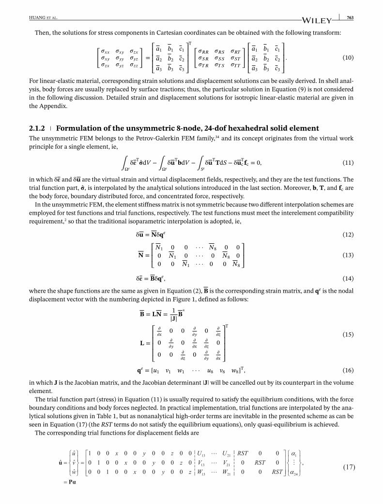
Then, the solutions for stress components in Cartesian coordinates can be obtained with the following transform:

[𝜎𝑥𝑥 𝜎𝑥𝑦 𝜎𝑧𝑥𝜎𝑥𝑦 𝜎𝑦𝑦 𝜎𝑦𝑧𝜎𝑧𝑥 𝜎𝑦𝑧 𝜎𝑧𝑧

]=

⎡⎢⎢⎢⎣a1 b1 c1

a2 b2 c2

a3 b3 c3

⎤⎥⎥⎥⎦T [

𝜎𝑅𝑅 𝜎𝑅𝑆 𝜎𝑅𝑇𝜎𝑆𝑅 𝜎𝑆𝑆 𝜎𝑆𝑇𝜎𝑇𝑅 𝜎𝑇𝑆 𝜎𝑇𝑇

] ⎡⎢⎢⎢⎣a1 b1 c1

a2 b2 c2

a3 b3 c3

⎤⎥⎥⎥⎦ . (10)

For linear-elastic material, corresponding strain solutions and displacement solutions can be easily derived. In shell anal-ysis, body forces are usually replaced by surface tractions; thus, the particular solution in Equation (9) is not consideredin the following discussion. Detailed strain and displacement solutions for isotropic linear-elastic material are given inthe Appendix.

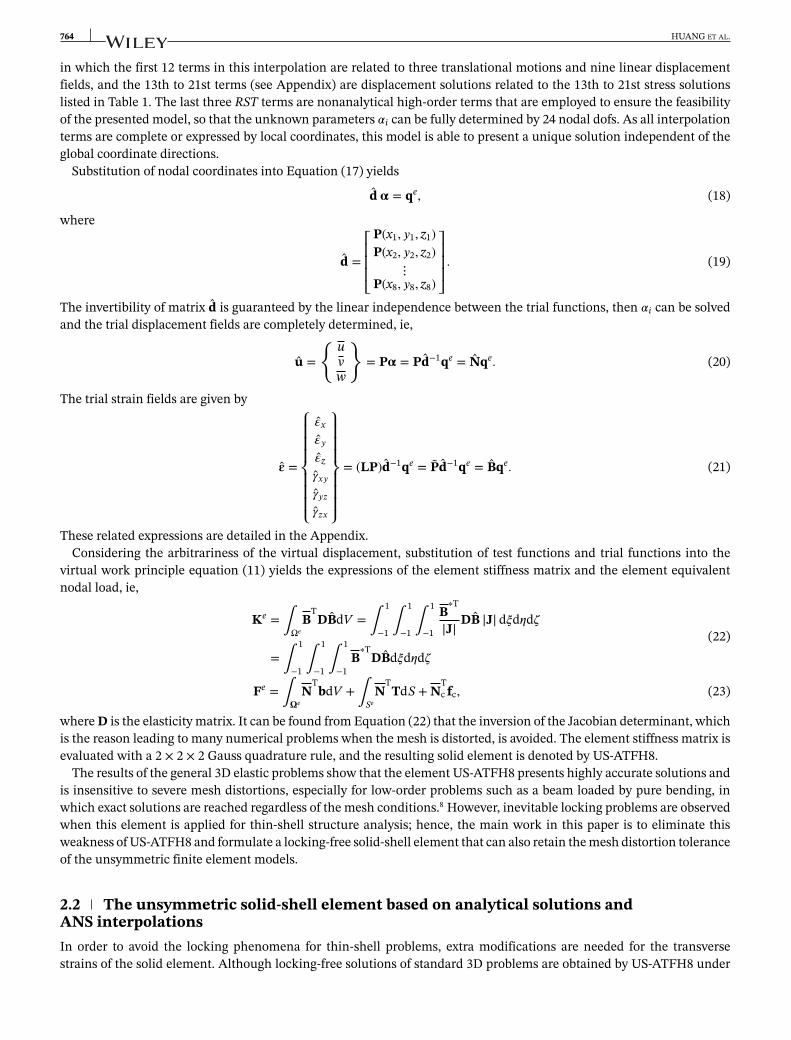
2.1.2 Formulation of the unsymmetric 8-node, 24-dof hexahedral solid elementThe unsymmetric FEM belongs to the Petrov-Galerkin FEM family,34 and its concept originates from the virtual workprinciple for a single element, ie,

∫Ωeδ𝛆T��dV − ∫Ωe

δuTbdV − ∫SeδuTTdS − δuT

c fc = 0, (11)

in which δ𝛆 and δu are the virtual strain and virtual displacement fields, respectively, and they are the test functions. Thetrial function part, ��, is interpolated by the analytical solutions introduced in the last section. Moreover, b, T, and fc arethe body force, boundary distributed force, and concentrated force, respectively.

In the unsymmetric FEM, the element stiffness matrix is not symmetric because two different interpolation schemes areemployed for test functions and trial functions, respectively. The test functions must meet the interelement compatibilityrequirement,2 so that the traditional isoparametric interpolation is adopted, ie,

δu = Nδqe (12)

N =⎡⎢⎢⎣

N1 0 0 · · · N8 0 00 N1 0 · · · 0 N8 00 0 N1 · · · 0 0 N8

⎤⎥⎥⎦ (13)

δ𝛆 = Bδqe, (14)

where the shape functions are the same as given in Equation (2), B is the corresponding strain matrix, and qe is the nodaldisplacement vector with the numbering depicted in Figure 1, defined as follows:

B = LN = 1|J|B∗

L =

⎡⎢⎢⎢⎢⎣𝜕

𝜕x0 0 𝜕

𝜕𝑦0 𝜕

𝜕z

0 𝜕

𝜕𝑦0 𝜕

𝜕x𝜕

𝜕z0

0 0 𝜕

𝜕z0 𝜕

𝜕𝑦

𝜕

𝜕x

⎤⎥⎥⎥⎥⎦

T

(15)

qe = [u1 v1 w1 · · · u8 v8 w8]T, (16)

in which J is the Jacobian matrix, and the Jacobian determinant |J| will be cancelled out by its counterpart in the volumeelement.

The trial function part (stress) in Equation (11) is usually required to satisfy the equilibrium conditions, with the forceboundary conditions and body forces neglected. In practical implementation, trial functions are interpolated by the ana-lytical solutions given in Table 1, but as nonanalytical high-order terms are inevitable in the presented scheme as can beseen in Equation (17) (the RST terms do not satisfy the equilibrium equations), only quasi-equilibrium is achieved.

The corresponding trial functions for displacement fields are

764 HUANG ET AL.

in which the first 12 terms in this interpolation are related to three translational motions and nine linear displacementfields, and the 13th to 21st terms (see Appendix) are displacement solutions related to the 13th to 21st stress solutionslisted in Table 1. The last three RST terms are nonanalytical high-order terms that are employed to ensure the feasibilityof the presented model, so that the unknown parameters 𝛼i can be fully determined by 24 nodal dofs. As all interpolationterms are complete or expressed by local coordinates, this model is able to present a unique solution independent of theglobal coordinate directions.

Substitution of nodal coordinates into Equation (17) yields

d 𝛂 = qe, (18)

where

d =⎡⎢⎢⎢⎣

P(x1, 𝑦1, z1)P(x2, 𝑦2, z2)

⋮P(x8, 𝑦8, z8)

⎤⎥⎥⎥⎦ . (19)

The invertibility of matrix d is guaranteed by the linear independence between the trial functions, then 𝛼i can be solvedand the trial displacement fields are completely determined, ie,

u =

{ uvw

}= P𝛂 = Pd−1qe = Nqe. (20)

The trial strain fields are given by

�� =

⎧⎪⎪⎪⎨⎪⎪⎪⎩

��x

��𝑦

��z

��𝑥𝑦

��𝑦𝑧

��𝑧𝑥

⎫⎪⎪⎪⎬⎪⎪⎪⎭= (LP)d−1qe = Pd−1qe = Bqe. (21)

These related expressions are detailed in the Appendix.Considering the arbitrariness of the virtual displacement, substitution of test functions and trial functions into the

virtual work principle equation (11) yields the expressions of the element stiffness matrix and the element equivalentnodal load, ie,

Ke = ∫ΩeB

TDBdV = ∫

1

−1 ∫1

−1 ∫1

−1

B∗T

|J| DB |J| d𝜉d𝜂d𝜁

= ∫1

−1 ∫1

−1 ∫1

−1B∗T

DBd𝜉d𝜂d𝜁(22)

Fe = ∫𝛀eN

TbdV + ∫Se

NT

TdS + NTc fc, (23)

where D is the elasticity matrix. It can be found from Equation (22) that the inversion of the Jacobian determinant, whichis the reason leading to many numerical problems when the mesh is distorted, is avoided. The element stiffness matrix isevaluated with a 2 × 2 × 2 Gauss quadrature rule, and the resulting solid element is denoted by US-ATFH8.

The results of the general 3D elastic problems show that the element US-ATFH8 presents highly accurate solutions andis insensitive to severe mesh distortions, especially for low-order problems such as a beam loaded by pure bending, inwhich exact solutions are reached regardless of the mesh conditions.8 However, inevitable locking problems are observedwhen this element is applied for thin-shell structure analysis; hence, the main work in this paper is to eliminate thisweakness of US-ATFH8 and formulate a locking-free solid-shell element that can also retain the mesh distortion toleranceof the unsymmetric finite element models.

2.2 The unsymmetric solid-shell element based on analytical solutions andANS interpolationsIn order to avoid the locking phenomena for thin-shell problems, extra modifications are needed for the transversestrains of the solid element. Although locking-free solutions of standard 3D problems are obtained by US-ATFH8 under

HUANG ET AL. 765

FIGURE 2 Natural coordinates in shell elements

different loading and mesh conditions, the coupling between membrane stresses and bending stresses and the complexityof geometry in thin-shell structures lead to severe shear, trapezoidal, and thickness locking problems.

A systematic study shows that the source of locking problems in US-ATFH8 comes from the test function part (isopara-metric interpolation). Therefore, the ANS interpolations are employed in this section to eliminate the existing lockingproblems, and an effective solid-shell element US-ATFHS8 is formulated.

The natural coordinates and element nodal numbering are depicted in Figure 2, in which 𝜁 denotes the thickness direc-tion. The 1-2-3-4 and 5-6-7-8 surfaces are the bottom surface and the top surface of the shell, respectively. For descriptionconvenience, the isoparametric interpolation is rewritten as follows:

u = Nq0 + 𝜁Nqn, (24)

where

N =[

N1I3 N2I3 N3I3 N4I3]

(25)

I3 =

[ 11

1

],

⎧⎪⎪⎪⎨⎪⎪⎪⎩

N1 = 14(1 − 𝜉)(1 − 𝜂)

N2 = 14(1 + 𝜉)(1 − 𝜂)

N3 = 14(1 + 𝜉)(1 + 𝜂)

N4 = 14(1 − 𝜉)(1 + 𝜂)

(26)

q0 =

⎧⎪⎪⎨⎪⎪⎩

12(u1 + u5)

12(u2 + u6)

12(u3 + u7)

12(u4 + u8)

⎫⎪⎪⎬⎪⎪⎭, qn =

⎧⎪⎪⎨⎪⎪⎩

12(−u1 + u5)

12(−u2 + u6)

12(−u3 + u7)

12(−u4 + u8)

⎫⎪⎪⎬⎪⎪⎭. (27)

The geometric description is similar, ie,

X = NX0 + 𝜁NXn, X0 =

⎧⎪⎪⎨⎪⎪⎩

12(X1 + X5)

12(X2 + X6)

12(X3 + X7)

12(X4 + X8)

⎫⎪⎪⎬⎪⎪⎭, Xn =

⎧⎪⎪⎨⎪⎪⎩

12(−X1 + X5)

12(−X2 + X6)

12(−X3 + X7)

12(−X4 + X8)

⎫⎪⎪⎬⎪⎪⎭, (28)

in which X is the coordinate vector, and Xi is the coordinate vector of the ith node.The strain tensor is given as follows:

𝛆 = 12(∇u + u∇) ⇒ 𝜀i𝑗gig𝑗 = 1

2

[gi 𝜕u𝜕𝜉i +

𝜕u𝜕𝜉i gi

]= 1

2

[gig𝑗

(g𝑗 ·

𝜕u𝜕𝜉i

)+

(𝜕u𝜕𝜉i · g𝑗

)g𝑗gi

], (29)

in which the Einstein summation convention is employed, and 𝜉1, 𝜉2, and 𝜉3 denote 𝜉, 𝜂, and 𝜁 , respectively. Hence, thecovariant strain components are

𝜀i𝑗 =12

(𝜕X𝜕𝜉i ·

𝜕u𝜕𝜉𝑗

+ 𝜕X𝜕𝜉𝑗

· 𝜕u𝜕𝜉i

)= 1

2

[(𝜕X𝜕𝜉i

)T𝜕u𝜕𝜉𝑗

+(𝜕X𝜕𝜉𝑗

)T𝜕u𝜕𝜉i

]. (30)

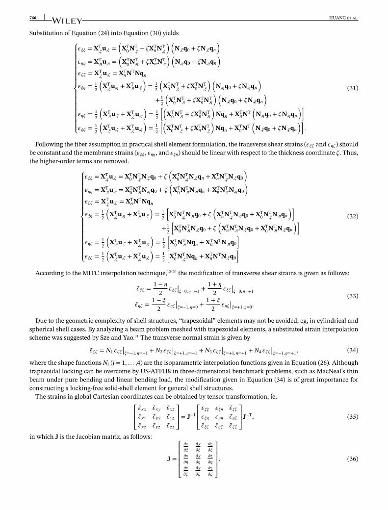
766 HUANG ET AL.

Substitution of Equation (24) into Equation (30) yields

⎧⎪⎪⎪⎪⎪⎪⎨⎪⎪⎪⎪⎪⎪⎩

𝜀𝜉𝜉 = XT,𝜉

u,𝜉 =(

XT0 NT

,𝜉+ 𝜁XT

nNT,𝜉

)(N,𝜉q0 + 𝜁N,𝜉qn

)𝜀𝜂𝜂 = XT

,𝜂u,𝜂 =(

XT0 NT

,𝜂 + 𝜁XTnNT

,𝜂

)(N,𝜂q0 + 𝜁N,𝜂qn

)𝜀𝜁𝜁 = XT

,𝜁u,𝜁 = XT

nNTNqn

𝜀𝜉𝜂 = 12

(XT,𝜉

u,𝜂 + XT,𝜂u,𝜉

)= 1

2

(XT

0 NT,𝜉+ 𝜁XT

nNT,𝜉

)(N,𝜂q0 + 𝜁N,𝜂qn

)+ 1

2

(XT

0 NT,𝜂 + 𝜁XT

nNT,𝜂

)(N,𝜉q0 + 𝜁N,𝜉qn

)𝜀𝜂𝜁 = 1

2

(XT,𝜂u,𝜁 + XT

,𝜁u,𝜂

)= 1

2

[(XT

0 NT,𝜂 + 𝜁XT

nNT,𝜂

)Nqn + XT

nNT(

N,𝜂q0 + 𝜁N,𝜂qn

)]𝜀𝜉𝜁 = 1

2

(XT,𝜉

u,𝜁 + XT,𝜁

u,𝜉

)= 1

2

[(XT

0 NT,𝜉+ 𝜁XT

nNT,𝜉

)Nqn + XT

nNT(

N,𝜉q0 + 𝜁N,𝜉qn

)].

(31)

Following the fiber assumption in practical shell element formulation, the transverse shear strains (𝜀𝜉𝜁 and 𝜀𝜂𝜁 ) shouldbe constant and the membrane strains (𝜀𝜉𝜉 , 𝜀𝜂𝜂 , and 𝜀𝜉𝜂) should be linear with respect to the thickness coordinate 𝜁 . Thus,the higher-order terms are removed.

⎧⎪⎪⎪⎪⎪⎪⎨⎪⎪⎪⎪⎪⎪⎩

𝜀𝜉𝜉 = XT,𝜉

u,𝜉 = XT0 NT

,𝜉N,𝜉q0 + 𝜁

(XT

0 NT,𝜉

N,𝜉qn + XTnNT

,𝜉N,𝜉q0

)𝜀𝜂𝜂 = XT

,𝜂u,𝜂 = XT0 NT

,𝜂N,𝜂q0 + 𝜁

(XT

0 NT,𝜂N,𝜂qn + XT

nNT,𝜂N,𝜂q0

)𝜀𝜁𝜁 = XT

,𝜁u,𝜁 = XT

nNTNqn

𝜀𝜉𝜂 = 12

(XT,𝜉

u,𝜂 + XT,𝜂u,𝜉

)= 1

2

[XT

0 NT,𝜉

N,𝜂q0 + 𝜁

(XT

nNT,𝜉

N,𝜂q0 + XT0 NT

,𝜉N,𝜂qn

)]+ 1

2

[XT

0 NT,𝜂N,𝜉q0 + 𝜁

(XT

nNT,𝜂N,𝜉q0 + XT

0 NT,𝜂N,𝜉qn

)]𝜀𝜂𝜁 = 1

2

(XT,𝜂u,𝜁 + XT

,𝜁u,𝜂

)= 1

2

[XT

0 NT,𝜂Nqn + XT

nNTN,𝜂q0

]𝜀𝜉𝜁 = 1

2

(XT,𝜉

u,𝜁 + XT,𝜁

u,𝜉

)= 1

2

[XT

0 NT,𝜉

Nqn + XTnNTN,𝜉q0

]

(32)

According to the MITC interpolation technique,12-20 the modification of transverse shear strains is given as follows:

��𝜉𝜁 =1 − 𝜂

2𝜀𝜉𝜁 ||𝜉=0, 𝜂=−1 +

1 + 𝜂

2𝜀𝜉𝜁 ||𝜉=0, 𝜂=+1

��𝜂𝜁 =1 − 𝜉

2𝜀𝜂𝜁 ||𝜉=−1, 𝜂=0 +

1 + 𝜉

2𝜀𝜂𝜁 ||𝜉=+1, 𝜂=0.

(33)

Due to the geometric complexity of shell structures, “trapezoidal” elements may not be avoided, eg, in cylindrical andspherical shell cases. By analyzing a beam problem meshed with trapezoidal elements, a substituted strain interpolationscheme was suggested by Sze and Yao.31 The transverse normal strain is given by

��𝜁𝜁 = N1 𝜀𝜁𝜁 ||𝜉=−1, 𝜂=−1 + N2 𝜀𝜁𝜁 ||𝜉=+1, 𝜂=−1 + N3 𝜀𝜁𝜁 ||𝜉=+1, 𝜂=+1 + N4 𝜀𝜁𝜁 ||𝜉=−1, 𝜂=+1, (34)

where the shape functions Ni (i = 1,… ,4) are the isoparametric interpolation functions given in Equation (26). Althoughtrapezoidal locking can be overcome by US-ATFH8 in three-dimensional benchmark problems, such as MacNeal's thinbeam under pure bending and linear bending load, the modification given in Equation (34) is of great importance forconstructing a locking-free solid-shell element for general shell structures.

The strains in global Cartesian coordinates can be obtained by tensor transformation, ie,⎡⎢⎢⎣��𝑥𝑥 ��𝑥𝑦 ��𝑥𝑧

��𝑥𝑦 ��𝑦𝑦 ��𝑦𝑧

��𝑥𝑧 ��𝑦𝑧 ��𝑧𝑧

⎤⎥⎥⎦ = J−1⎡⎢⎢⎣𝜀𝜉𝜉 𝜀𝜉𝜂 ��𝜉𝜁

𝜀𝜉𝜂 𝜀𝜂𝜂 ��𝜂𝜁

��𝜉𝜁 ��𝜂𝜁 ��𝜁𝜁

⎤⎥⎥⎦ J−T, (35)

in which J is the Jacobian matrix, as follows:

J =

⎡⎢⎢⎢⎢⎣𝜕x𝜕𝜉

𝜕𝑦

𝜕𝜉

𝜕z𝜕𝜉

𝜕x𝜕𝜂

𝜕𝑦

𝜕𝜂

𝜕z𝜕𝜂

𝜕x𝜕𝜁

𝜕𝑦

𝜕𝜁

𝜕z𝜕𝜁

⎤⎥⎥⎥⎥⎦. (36)

HUANG ET AL. 767

Thus, the virtual strain interpolation for an unsymmetric solid-shell element can be written in the following matrix form:

𝛿�� = B𝛿qe. (37)

The test function part in Equation (22) is replaced by the modified formulas, and the trial function part (stress inter-polation) remains the same. Hence, the element stiffness matrix of the solid-shell element (denoted by US-ATFHS8) isobtained as

Ke = ∫ΩeBTDBdV = ∫

1

−1 ∫1

−1 ∫1

−1BTDB|J|d𝜉d𝜂d𝜁. (38)

It should be noted that a 1/|J|2 term is contained in the B matrix, so that inversion of the Jacobian determinant is neededin computing the element stiffness matrix, which will weaken the mesh distortion tolerance of the unsymmetric finiteelements. Such imperfection cannot be overcome unless the modification is conducted without the help of natural coor-dinates. Despite this weakness, remarkable mesh distortion tolerance is still presented by this locking-free solid-shellmodel, and this will be shown in the next section.

The 2 × 2 × 2 Gauss quadrature rule for Equation (38) is still proved to be sufficient in computer coding. Althoughremarkable mesh distortion tolerance is inherited from US-ATFH8, US-ATFHS8 is not recommended for the elementsof which the top and bottom surfaces are degenerated triangles or concave quadrilaterals to prevent the Jacobiandeterminant from vanishing.

3 NUMERICAL EXAMPLES

Nine numerical tests are presented in this section to demonstrate the performance of the proposed element US-ATFHS8.The results obtained by some other elements are also given for comparison. These elements referred to are as follows:

ANSγε: a solid-shell model using ANS techniques introduced by Sze and Yao31;ANSγε-HS: a hybrid-stress solid-shell model based on the ANSγε model proposed by Sze and Yao31;SC8R: a (reduced integration) solid-shell element assembled in commercial software Abaqus.35

It should be noted that the displacement solutions solved by ANSγε and ANSγε-HS are calculated by the authors usingthe formulation in the work of Sze and Yao.31 Due to some distinctions in modeling and programming, for example, thenumber of Gaussian points employed in one element (2 × 2 points for the presented results), the presented data are notcompletely identical to those given by Sze and Yao,31 but these differences are negligible and reasonable (and these twoelements are also verified by patch tests).

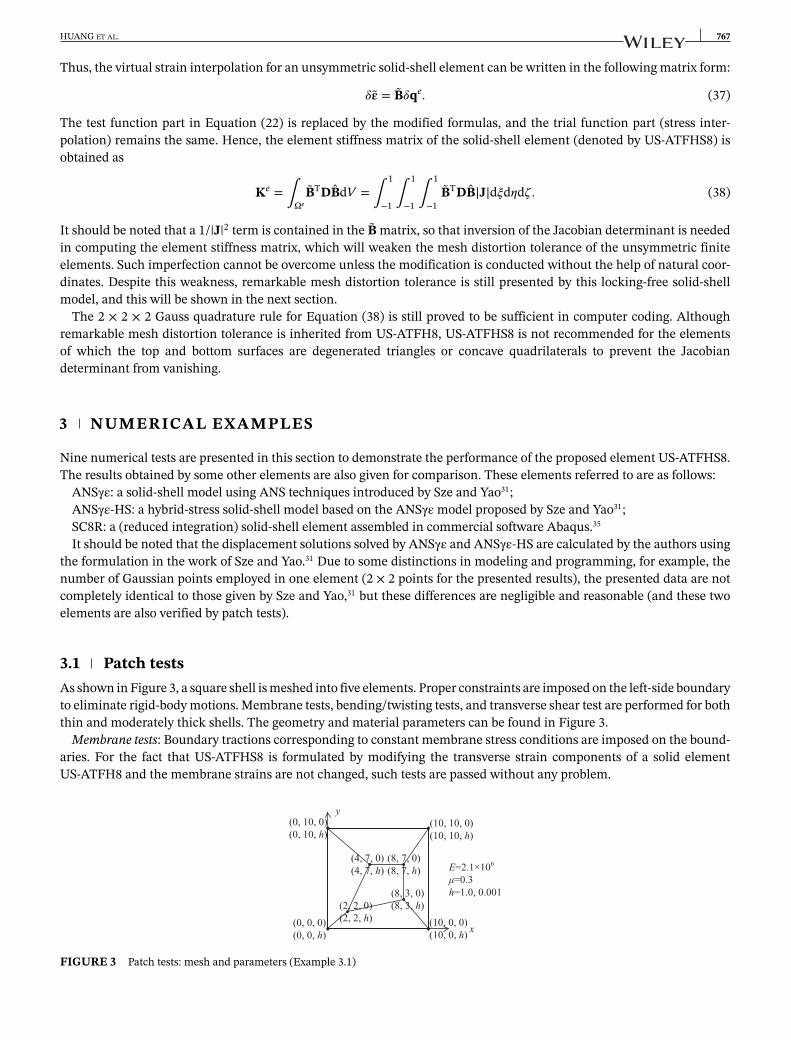
3.1 Patch testsAs shown in Figure 3, a square shell is meshed into five elements. Proper constraints are imposed on the left-side boundaryto eliminate rigid-body motions. Membrane tests, bending/twisting tests, and transverse shear test are performed for boththin and moderately thick shells. The geometry and material parameters can be found in Figure 3.

Membrane tests: Boundary tractions corresponding to constant membrane stress conditions are imposed on the bound-aries. For the fact that US-ATFHS8 is formulated by modifying the transverse strain components of a solid elementUS-ATFH8 and the membrane strains are not changed, such tests are passed without any problem.

FIGURE 3 Patch tests: mesh and parameters (Example 3.1)

768 HUANG ET AL.

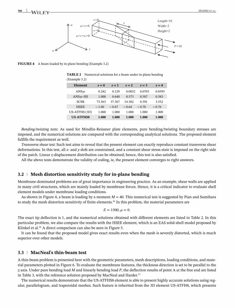
FIGURE 4 A beam loaded by in-plane bending (Example 3.2)

TABLE 2 Numerical solutions for a beam under in-plane bending(Example 3.2)

Element s = 0 s = 1 s = 2 s = 3 s = 4

ANSγε 0.242 0.129 0.0852 0.0703 0.0595ANSγε-HS 1.000 0.640 0.573 0.587 0.583

SC8R 73.563 37.367 14.302 6.591 3.552HSEE ∼ 1.00 ∼ 0.67 ∼ 0.64 ∼ 0.70 ∼ 0.76

US-ATFH8 (3D) 1.000 1.000 1.000 1.000 1.000US-ATFHS8 1.000 1.000 1.000 1.000 1.000

Bending/twisting tests: As used for Mindlin-Reissner plate elements, pure bending/twisting boundary stresses areimposed, and the numerical solutions are compared with the corresponding analytical solutions. The proposed elementfulfills the requirement as well.

Transverse shear test: Such test aims to reveal that the present element can exactly reproduce constant transverse sheardeformations. In this test, all x- and y-dofs are constrained, and a constant shear stress state is imposed on the right sideof the patch. Linear z-displacement distribution can be obtained; hence, this test is also satisfied.

All the above tests demonstrate the validity of coding, ie, the present element converges to right answers.

3.2 Mesh distortion sensitivity study for in-plane bendingMembrane-dominated problems are of great importance in engineering practice. As an example, shear walls are appliedin many civil structures, which are mainly loaded by membrane forces. Hence, it is a critical indicator to evaluate shellelement models under membrane loading conditions.

As shown in Figure 4, a beam is loading by a moment M = 40. This numerical test is suggested by Pian and Sumiharato study the mesh distortion sensitivity of finite elements.36 In this problem, the material parameters are

E = 1500, 𝜇 = 0.

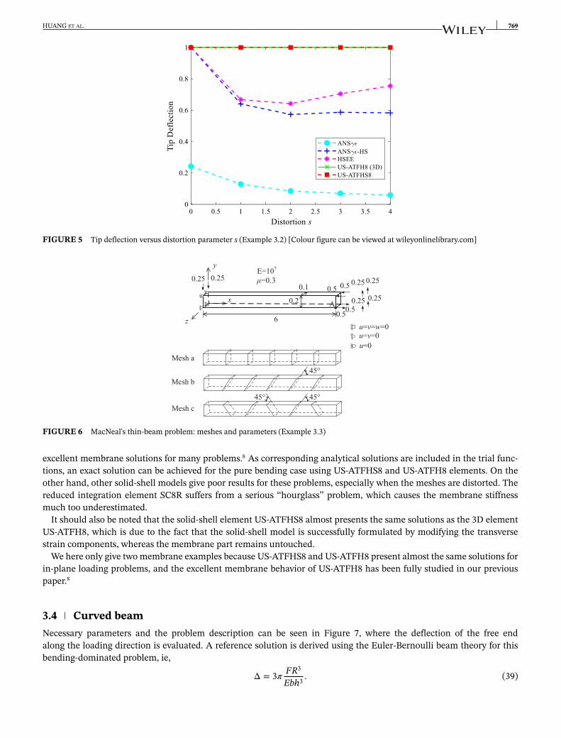
The exact tip deflection is 1, and the numerical solutions obtained with different elements are listed in Table 2. In thisparticular problem, we also compare the results with the HSEE element, which is an EAS solid-shell model proposed byKlinkel et al.26 A direct comparison can also be seen in Figure 5.

It can be found that the proposed model gives exact results even when the mesh is severely distorted, which is muchsuperior over other models.

3.3 MacNeal's thin-beam testA thin-beam problem is presented here with the geometric parameters, mesh descriptions, loading conditions, and mate-rial parameters plotted in Figure 6. To evaluate the membrane features, the thickness direction is set to be parallel to thez-axis. Under pure bending load M and linearly bending load P, the deflection results of point A at the free end are listedin Table 3, with the reference solution proposed by MacNeal and Harder.37

The numerical results demonstrate that the US-ATFHS8 element is able to present highly accurate solutions using reg-ular, parallelogram, and trapezoidal meshes. Such feature is inherited from the 3D element US-ATFH8, which presents

HUANG ET AL. 769

FIGURE 5 Tip deflection versus distortion parameter s (Example 3.2) [Colour figure can be viewed at wileyonlinelibrary.com]

FIGURE 6 MacNeal's thin-beam problem: meshes and parameters (Example 3.3)

excellent membrane solutions for many problems.8 As corresponding analytical solutions are included in the trial func-tions, an exact solution can be achieved for the pure bending case using US-ATFHS8 and US-ATFH8 elements. On theother hand, other solid-shell models give poor results for these problems, especially when the meshes are distorted. Thereduced integration element SC8R suffers from a serious “hourglass” problem, which causes the membrane stiffnessmuch too underestimated.

It should also be noted that the solid-shell element US-ATFHS8 almost presents the same solutions as the 3D elementUS-ATFH8, which is due to the fact that the solid-shell model is successfully formulated by modifying the transversestrain components, whereas the membrane part remains untouched.

We here only give two membrane examples because US-ATFHS8 and US-ATFH8 present almost the same solutions forin-plane loading problems, and the excellent membrane behavior of US-ATFH8 has been fully studied in our previouspaper.8

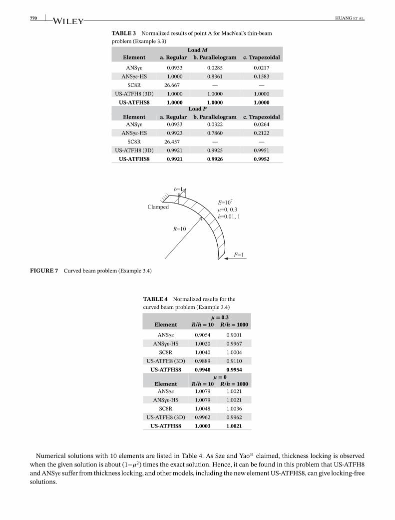
3.4 Curved beamNecessary parameters and the problem description can be seen in Figure 7, where the deflection of the free endalong the loading direction is evaluated. A reference solution is derived using the Euler-Bernoulli beam theory for thisbending-dominated problem, ie,

Δ = 3𝜋 FR3

Ebh3 . (39)

http://wileyonlinelibrary.com

770 HUANG ET AL.

TABLE 3 Normalized results of point A for MacNeal's thin-beamproblem (Example 3.3)

Load MElement a. Regular b. Parallelogram c. Trapezoidal

ANSγε 0.0933 0.0285 0.0217ANSγε-HS 1.0000 0.8361 0.1583

SC8R 26.667 — —US-ATFH8 (3D) 1.0000 1.0000 1.0000

US-ATFHS8 1.0000 1.0000 1.0000Load P

Element a. Regular b. Parallelogram c. TrapezoidalANSγε 0.0933 0.0322 0.0264

ANSγε-HS 0.9923 0.7860 0.2122SC8R 26.457 — —

US-ATFH8 (3D) 0.9921 0.9925 0.9951US-ATFHS8 0.9921 0.9926 0.9952

FIGURE 7 Curved beam problem (Example 3.4)

TABLE 4 Normalized results for thecurved beam problem (Example 3.4)

𝝁 = 0.3Element R/h = 10 R/h = 1000

ANSγε 0.9054 0.9001ANSγε-HS 1.0020 0.9967

SC8R 1.0040 1.0004US-ATFH8 (3D) 0.9889 0.9110

US-ATFHS8 0.9940 0.9954𝝁 = 0

Element R/h = 10 R/h = 1000ANSγε 1.0079 1.0021

ANSγε-HS 1.0079 1.0021SC8R 1.0048 1.0036

US-ATFH8 (3D) 0.9962 0.9962US-ATFHS8 1.0003 1.0021

Numerical solutions with 10 elements are listed in Table 4. As Sze and Yao31 claimed, thickness locking is observedwhen the given solution is about (1−𝜇2) times the exact solution. Hence, it can be found in this problem that US-ATFH8and ANSγε suffer from thickness locking, and other models, including the new element US-ATFHS8, can give locking-freesolutions.

HUANG ET AL. 771

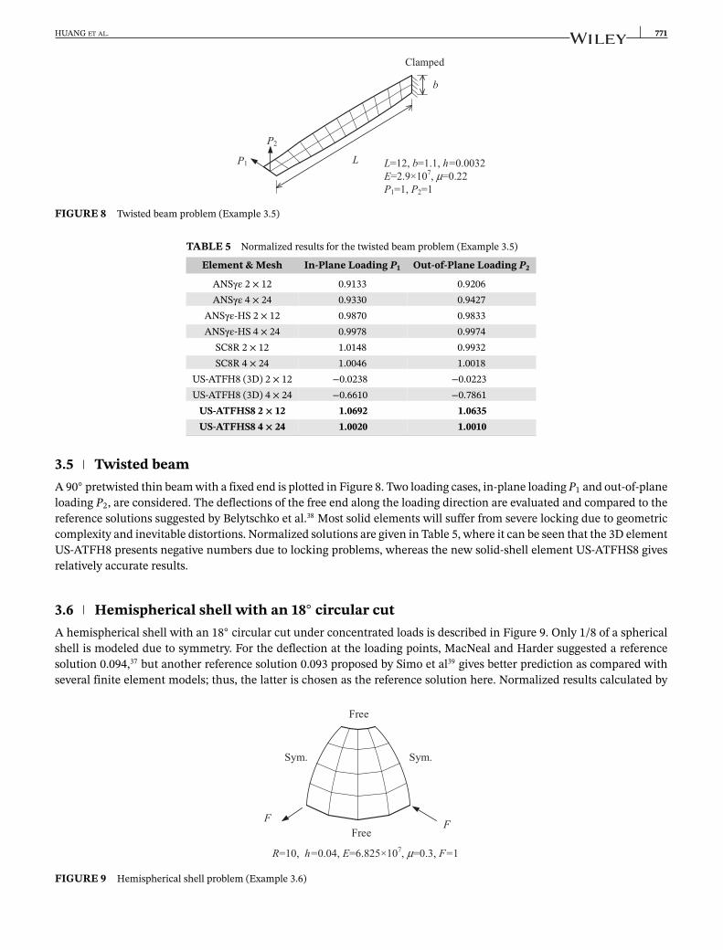
FIGURE 8 Twisted beam problem (Example 3.5)

TABLE 5 Normalized results for the twisted beam problem (Example 3.5)

Element & Mesh In-Plane Loading P1 Out-of-Plane Loading P2

ANSγε 2 × 12 0.9133 0.9206ANSγε 4 × 24 0.9330 0.9427

ANSγε-HS 2 × 12 0.9870 0.9833ANSγε-HS 4 × 24 0.9978 0.9974

SC8R 2 × 12 1.0148 0.9932SC8R 4 × 24 1.0046 1.0018

US-ATFH8 (3D) 2 × 12 −0.0238 −0.0223US-ATFH8 (3D) 4 × 24 −0.6610 −0.7861

US-ATFHS8 2 × 12 1.0692 1.0635US-ATFHS8 4 × 24 1.0020 1.0010

3.5 Twisted beamA 90◦ pretwisted thin beam with a fixed end is plotted in Figure 8. Two loading cases, in-plane loading P1 and out-of-planeloading P2, are considered. The deflections of the free end along the loading direction are evaluated and compared to thereference solutions suggested by Belytschko et al.38 Most solid elements will suffer from severe locking due to geometriccomplexity and inevitable distortions. Normalized solutions are given in Table 5, where it can be seen that the 3D elementUS-ATFH8 presents negative numbers due to locking problems, whereas the new solid-shell element US-ATFHS8 givesrelatively accurate results.

3.6 Hemispherical shell with an 18◦ circular cutA hemispherical shell with an 18◦ circular cut under concentrated loads is described in Figure 9. Only 1/8 of a sphericalshell is modeled due to symmetry. For the deflection at the loading points, MacNeal and Harder suggested a referencesolution 0.094,37 but another reference solution 0.093 proposed by Simo et al39 gives better prediction as compared withseveral finite element models; thus, the latter is chosen as the reference solution here. Normalized results calculated by

FIGURE 9 Hemispherical shell problem (Example 3.6)

772 HUANG ET AL.

TABLE 6 Normalized results for thehemispherical shell problem (Example 3.6)

Element 4 × 4 8 × 8 16 × 16

ANSγε 1.0333 1.0051 0.9983ANSγε-HS 1.0624 1.0148 1.0052

SC8R 1.1594 1.0435 1.0154US-ATFH8 (3D) 0.0186 0.2150 0.7995

US-ATFHS8 1.1031 1.0106 1.0038

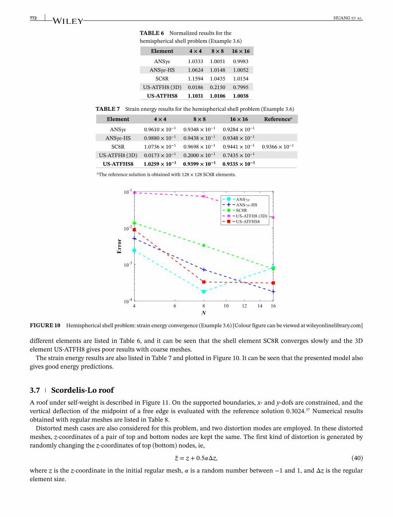
TABLE 7 Strain energy results for the hemispherical shell problem (Example 3.6)

Element 4 × 4 8 × 8 16 × 16 Referencea

ANSγε 0.9610 × 10−1 0.9348 × 10−1 0.9284 × 10−1

ANSγε-HS 0.9880 × 10−1 0.9438 × 10−1 0.9348 × 10−1

SC8R 1.0736 × 10−1 0.9698 × 10−1 0.9441 × 10−1 0.9366 × 10−1

US-ATFH8 (3D) 0.0173 × 10−1 0.2000 × 10−1 0.7435 × 10−1

US-ATFHS8 1.0259 × 10−1 0.9399 × 10−1 0.9335 × 10−1

aThe reference solution is obtained with 128 × 128 SC8R elements.

FIGURE 10 Hemispherical shell problem: strain energy convergence (Example 3.6) [Colour figure can be viewed at wileyonlinelibrary.com]

different elements are listed in Table 6, and it can be seen that the shell element SC8R converges slowly and the 3Delement US-ATFH8 gives poor results with coarse meshes.

The strain energy results are also listed in Table 7 and plotted in Figure 10. It can be seen that the presented model alsogives good energy predictions.

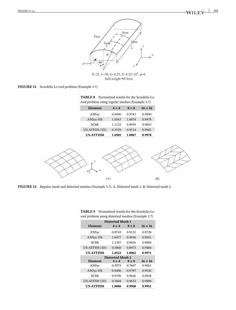
3.7 Scordelis-Lo roofA roof under self-weight is described in Figure 11. On the supported boundaries, x- and y-dofs are constrained, and thevertical deflection of the midpoint of a free edge is evaluated with the reference solution 0.3024.37 Numerical resultsobtained with regular meshes are listed in Table 8.

Distorted mesh cases are also considered for this problem, and two distortion modes are employed. In these distortedmeshes, z-coordinates of a pair of top and bottom nodes are kept the same. The first kind of distortion is generated byrandomly changing the z-coordinates of top (bottom) nodes, ie,

z = z + 0.5𝛼Δz, (40)

where z is the z-coordinate in the initial regular mesh, 𝛼 is a random number between −1 and 1, and Δz is the regularelement size.


HUANG ET AL. 773

FIGURE 11 Scordelis-Lo roof problem (Example 3.7)

TABLE 8 Normalized results for the Scordelis-Loroof problem using regular meshes (Example 3.7)

Element 4 × 4 8 × 8 16 × 16

ANSγε 0.9496 0.9743 0.9890ANSγε-HS 1.0565 1.0074 0.9978

SC8R 1.1122 0.9959 0.9893US-ATFH8 (3D) 0.5529 0.9514 0.9941

US-ATFHS8 1.0505 1.0067 0.9978

x

y

z

(A) (B)

FIGURE 12 Regular mesh and distorted meshes (Example 3.7). A, Distorted mesh 1; B, Distorted mesh 2

TABLE 9 Normalized results for the Scordelis-Loroof problem using distorted meshes (Example 3.7)

Distorted Mesh 1Element 4 × 4 8 × 8 16 × 16

ANSγε 0.8743 0.9132 0.9728ANSγε-HS 1.0477 0.9936 0.9921

SC8R 1.1307 0.9816 0.9868US-ATFH8 (3D) 0.5860 0.8973 0.9486

US-ATFHS8 1.0522 1.0062 0.9971Distorted Mesh 2

Element 4 × 4 8 × 8 16 × 16ANSγε 0.5973 0.7607 0.9061

ANSγε-HS 0.9496 0.9797 0.9926SC8R 0.9796 0.9626 0.9828

US-ATFH8 (3D) 0.5604 0.9633 0.9909US-ATFHS8 1.0086 0.9960 0.9951

774 HUANG ET AL.

TABLE 10 Strain energy results for the Scordelis-Lo roof problem (Example 3.7)Regular Mesh Referencea

Element 4 × 4 8 × 8 16 × 16

ANSγε 0.1126 × 104 0.1175 × 104 0.1198 × 104

ANSγε-HS 0.1264 × 104 0.1218 × 104 0.1210 × 104

SC8R 0.1314 × 104 0.1196 × 104 0.1197 × 104

US-ATFH8 (3D) 0.0779 × 104 0.1162 × 104 0.1206 × 104

US-ATFHS8 0.1254 × 104 0.1217 × 104 0.1210 × 104


ANSγε 0.1022 × 104 0.1104 × 104 0.1177 × 104

ANSγε-HS 0.1241 × 104 0.1198 × 104 0.1202 × 104

SC8R 0.1323 × 104 0.1182 × 104 0.1193 × 104 0.1209 × 104

US-ATFH8 (3D) 0.0787 × 104 0.1054 × 104 0.1147 × 104

US-ATFHS8 0.1249 × 104 0.1214 × 104 0.1208 × 104


ANSγε 0.0642 × 104 0.0873 × 104 0.1080 × 104

ANSγε-HS 0.1136 × 104 0.1192 × 104 0.1206 × 104

SC8R 0.1144 × 104 0.1163 × 104 0.1191 × 104

US-ATFH8 (3D) 0.0830 × 104 0.1181 × 104 0.1205 × 104

US-ATFHS8 0.1215 × 104 0.1205 × 104 0.1207 × 104

aThe reference solution is obtained with 128 × 128 SC8R elements.

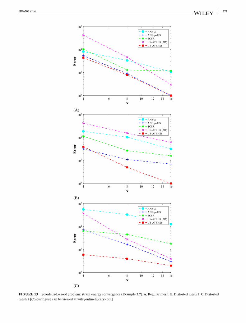
The second kind of distortion changes the random number 𝛼 to be an assigned value for each top (bottom) node. Fordifferent nodes with the same x and y coordinates (they are in a row), the values of 𝛼 are also the same. For differentnodes in two adjacent rows, the values of 𝛼 are taken to be 1 and −1, respectively. Regular mesh and two kinds of distortedmeshes discretized with 4 × 4 elements are also plotted in Figure 12, and the numerical results using distorted meshes aregiven in Table 9. To better understand the convergence, the corresponding strain energy results are presented in Table 10and visualized in Figure 13.

It is clear that the proposed solid-shell element US-ATFHS8 gives remarkable (local and global) results under bothregular and distorted meshes, and these solutions are not sensitive to mesh distortions. Rapid energy convergence isalways achieved by the proposed model under various mesh conditions.

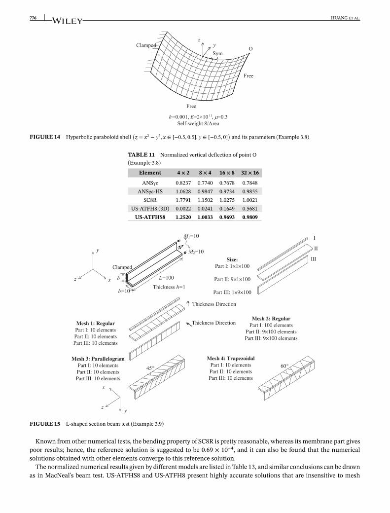
3.8 Partly clamped hyperbolic paraboloid shellThe geometric and material parameters of a partly clamped hyperbolic paraboloid shell loaded by its self-weight areplotted in Figure 14. The reference solution for this problem is given by Bathe et al using a high-order MITC model.16 Thevertical deflection at point O is evaluated, and the numerical results are given in Table 11. It can be seen that the SC8Rmodel gives much larger solutions in coarse meshes, which is due to the reduced integration.

3.9 A beam with an L-shaped cross sectionAs depicted in Figure 15, an L-shaped section beam is loaded by two bending moments at its free end. To illustrate themesh and thickness directions of shell elements, this beam is divided into three parts (two plates and one ridge). Thematerial parameters are as follows:

E = 107, 𝜇 = 0.3.The geometrical data are all given in the Figure, and the assigned moment is implemented by using concentrated forces.The x- and y-deflections at the outer angular point, where the largest displacement should be observed, are evaluated inthis test.

Four meshes are considered, of which three are coarse meshes discretized with 30 elements and one is a fine mesh forconvergence analysis. Both the parallelogram mesh and trapezoidal mesh are used to check the mesh distortion sensitivity.

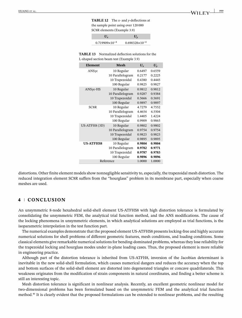
The reference solution is obtained by using over 120 000 SC8R elements (4 × 36 × 400 elements for part II and part IIIand 4 × 4 × 400 elements for part I). It is observed in Table 12 that although so many elements are used, the x- andy-deflections at the sample point are clearly different, while they are analytically identical due to the symmetry.

HUANG ET AL. 775

(A)

(B)

(C)

FIGURE 13 Scordelis-Lo roof problem: strain energy convergence (Example 3.7). A, Regular mesh; B, Distorted mesh 1; C, Distortedmesh 2 [Colour figure can be viewed at wileyonlinelibrary.com]


776 HUANG ET AL.

FIGURE 14 Hyperbolic paraboloid shell(

z = x2 − 𝑦2, x ∈ [−0.5, 0.5], 𝑦 ∈ [−0.5, 0])

and its parameters (Example 3.8)

TABLE 11 Normalized vertical deflection of point O(Example 3.8)

Element 4 × 2 8 × 4 16 × 8 32 × 16

ANSγε 0.8237 0.7740 0.7678 0.7848ANSγε-HS 1.0628 0.9847 0.9734 0.9855

SC8R 1.7791 1.1502 1.0275 1.0021US-ATFH8 (3D) 0.0022 0.0241 0.1649 0.5681

US-ATFHS8 1.2520 1.0033 0.9693 0.9809

Size:Part I: 1×1×100

Part II: 9×1×100

Part III: 1×9×100

x

y

z L=100

b=10

bThickness h=1

Clamped

M1=10

M2=10

Mesh 1: RegularPart I: 10 elementsPart II: 10 elementsPart III: 10 elements

Thickness Direction

Mesh 2: RegularPart I: 100 elements

Part II: 9×100 elementsPart III: 9×100 elements

Mesh 3: ParallelogramPart I: 10 elementsPart II: 10 elementsPart III: 10 elements

Mesh 4: TrapezoidalPart I: 10 elementsPart II: 10 elementsPart III: 10 elements

x

yz

45° 60°

Thickness Direction

I

II

III

FIGURE 15 L-shaped section beam test (Example 3.9)

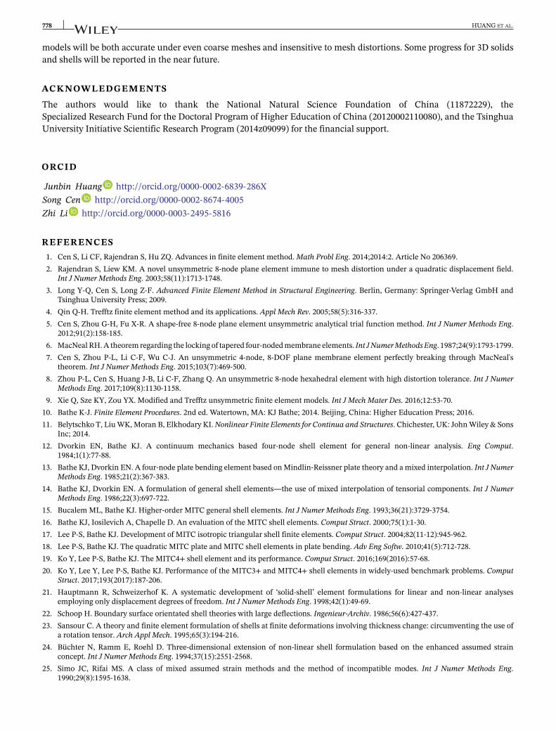
Known from other numerical tests, the bending property of SC8R is pretty reasonable, whereas its membrane part givespoor results; hence, the reference solution is suggested to be 0.69 × 10−4, and it can also be found that the numericalsolutions obtained with other elements converge to this reference solution.

The normalized numerical results given by different models are listed in Table 13, and similar conclusions can be drawnas in MacNeal's beam test. US-ATFHS8 and US-ATFH8 present highly accurate solutions that are insensitive to mesh

HUANG ET AL. 777

TABLE 12 The x- and y-deflections atthe sample point using over 120 000SC8R elements (Example 3.9)

Ux Uy

0.719909×10−4 0.690328×10−4

TABLE 13 Normalized deflection solutions for theL-shaped section beam test (Example 3.9)

Element Mesh Ux Uy

ANSγε 10 Regular 0.6497 0.655910 Parallelogram 0.2177 0.222510 Trapezoidal 0.4380 0.4445

100 Regular 0.9825 0.9827ANSγε-HS 10 Regular 0.9812 0.9812

10 Parallelogram 0.9287 0.938410 Trapezoidal 0.5666 0.5691

100 Regular 0.9897 0.9897SC8R 10 Regular 4.7279 4.7552


100 Regular 0.9909 0.9865US-ATFH8 (3D) 10 Regular 0.9802 0.9802


100 Regular 0.9895 0.9895US-ATFHS8 10 Regular 0.9804 0.9804


100 Regular 0.9896 0.9896Reference 1.0000 1.0000

distortions. Other finite element models show nonnegligible sensitivity to, especially, the trapezoidal mesh distortion. Thereduced integration element SC8R suffers from the “hourglass” problem in its membrane part, especially when coarsemeshes are used.

4 CONCLUSION

An unsymmetric 8-node hexahedral solid-shell element US-ATFHS8 with high distortion tolerance is formulated byconsolidating the unsymmetric FEM, the analytical trial function method, and the ANS modifications. The cause ofthe locking phenomena in unsymmetric elements, in which analytical solutions are employed as trial functions, is theisoparametric interpolation in the test function part.

The numerical examples demonstrate that the proposed element US-ATFHS8 presents locking-free and highly accuratenumerical solutions for shell problems of different geometric features, mesh conditions, and loading conditions. Someclassical elements give remarkable numerical solutions for bending-dominated problems, whereas they lose reliability forthe trapezoidal locking and hourglass modes under in-plane loading cases. Thus, the proposed element is more reliablein engineering practice.

Although part of the distortion tolerance is inherited from US-ATFH8, inversion of the Jacobian determinant isinevitable in the new solid-shell formulation, which causes numerical dangers and reduces the accuracy when the topand bottom surfaces of the solid-shell element are distorted into degenerated triangles or concave quadrilaterals. Thisweakness originates from the modification of strain components in natural coordinates, and finding a better scheme isstill an interesting topic.

Mesh distortion tolerance is significant in nonlinear analysis. Recently, an excellent geometric nonlinear model fortwo-dimensional problems has been formulated based on the unsymmetric FEM and the analytical trial functionmethod.40 It is clearly evident that the proposed formulations can be extended to nonlinear problems, and the resulting

778 HUANG ET AL.

models will be both accurate under even coarse meshes and insensitive to mesh distortions. Some progress for 3D solidsand shells will be reported in the near future.

ACKNOWLEDGEMENTS

The authors would like to thank the National Natural Science Foundation of China (11872229), theSpecialized Research Fund for the Doctoral Program of Higher Education of China (20120002110080), and the TsinghuaUniversity Initiative Scientific Research Program (2014z09099) for the financial support.

ORCID

Junbin Huang http://orcid.org/0000-0002-6839-286XSong Cen http://orcid.org/0000-0002-8674-4005Zhi Li http://orcid.org/0000-0003-2495-5816

REFERENCES1. Cen S, Li CF, Rajendran S, Hu ZQ. Advances in finite element method. Math Probl Eng. 2014;2014:2. Article No 206369.2. Rajendran S, Liew KM. A novel unsymmetric 8-node plane element immune to mesh distortion under a quadratic displacement field.

Int J Numer Methods Eng. 2003;58(11):1713-1748.3. Long Y-Q, Cen S, Long Z-F. Advanced Finite Element Method in Structural Engineering. Berlin, Germany: Springer-Verlag GmbH and

Tsinghua University Press; 2009.4. Qin Q-H. Trefftz finite element method and its applications. Appl Mech Rev. 2005;58(5):316-337.5. Cen S, Zhou G-H, Fu X-R. A shape-free 8-node plane element unsymmetric analytical trial function method. Int J Numer Methods Eng.

2012;91(2):158-185.6. MacNeal RH. A theorem regarding the locking of tapered four-noded membrane elements. Int J Numer Methods Eng. 1987;24(9):1793-1799.7. Cen S, Zhou P-L, Li C-F, Wu C-J. An unsymmetric 4-node, 8-DOF plane membrane element perfectly breaking through MacNeal's

theorem. Int J Numer Methods Eng. 2015;103(7):469-500.8. Zhou P-L, Cen S, Huang J-B, Li C-F, Zhang Q. An unsymmetric 8-node hexahedral element with high distortion tolerance. Int J Numer

Methods Eng. 2017;109(8):1130-1158.9. Xie Q, Sze KY, Zou YX. Modified and Trefftz unsymmetric finite element models. Int J Mech Mater Des. 2016;12:53-70.

10. Bathe K-J. Finite Element Procedures. 2nd ed. Watertown, MA: KJ Bathe; 2014. Beijing, China: Higher Education Press; 2016.11. Belytschko T, Liu WK, Moran B, Elkhodary KI. Nonlinear Finite Elements for Continua and Structures. Chichester, UK: John Wiley & Sons

Inc; 2014.12. Dvorkin EN, Bathe KJ. A continuum mechanics based four-node shell element for general non-linear analysis. Eng Comput.

1984;1(1):77-88.13. Bathe KJ, Dvorkin EN. A four-node plate bending element based on Mindlin-Reissner plate theory and a mixed interpolation. Int J Numer

Methods Eng. 1985;21(2):367-383.14. Bathe KJ, Dvorkin EN. A formulation of general shell elements—the use of mixed interpolation of tensorial components. Int J Numer

Methods Eng. 1986;22(3):697-722.15. Bucalem ML, Bathe KJ. Higher-order MITC general shell elements. Int J Numer Methods Eng. 1993;36(21):3729-3754.16. Bathe KJ, Iosilevich A, Chapelle D. An evaluation of the MITC shell elements. Comput Struct. 2000;75(1):1-30.17. Lee P-S, Bathe KJ. Development of MITC isotropic triangular shell finite elements. Comput Struct. 2004;82(11-12):945-962.18. Lee P-S, Bathe KJ. The quadratic MITC plate and MITC shell elements in plate bending. Adv Eng Softw. 2010;41(5):712-728.19. Ko Y, Lee P-S, Bathe KJ. The MITC4+ shell element and its performance. Comput Struct. 2016;169(2016):57-68.20. Ko Y, Lee Y, Lee P-S, Bathe KJ. Performance of the MITC3+ and MITC4+ shell elements in widely-used benchmark problems. Comput

Struct. 2017;193(2017):187-206.21. Hauptmann R, Schweizerhof K. A systematic development of ‘solid-shell’ element formulations for linear and non-linear analyses

employing only displacement degrees of freedom. Int J Numer Methods Eng. 1998;42(1):49-69.22. Schoop H. Boundary surface orientated shell theories with large deflections. Ingenieur-Archiv. 1986;56(6):427-437.23. Sansour C. A theory and finite element formulation of shells at finite deformations involving thickness change: circumventing the use of

a rotation tensor. Arch Appl Mech. 1995;65(3):194-216.24. Büchter N, Ramm E, Roehl D. Three-dimensional extension of non-linear shell formulation based on the enhanced assumed strain

concept. Int J Numer Methods Eng. 1994;37(15):2551-2568.25. Simo JC, Rifai MS. A class of mixed assumed strain methods and the method of incompatible modes. Int J Numer Methods Eng.

1990;29(8):1595-1638.

http://orcid.org/0000-0002-6839-286X

http://orcid.org/0000-0002-6839-286X

http://orcid.org/0000-0002-8674-4005

http://orcid.org/0000-0002-8674-4005

http://orcid.org/0000-0003-2495-5816

http://orcid.org/0000-0003-2495-5816

HUANG ET AL. 779

26. Klinkel S, Gruttmann F, Wagner W. A robust non-linear solid shell element based on a mixed variational formulation. Comput MethodsAppl Mech Eng. 2006;195(1-3):179-201.

27. Reese S. A large deformation solid-shell concept based on reduced integration with hourglass stabilization. Int J Numer Methods Eng.2007;69(8):1671-1716.

28. Parisch H. A continuum-based shell theory for non-linear applications. Int J Numer Methods Eng. 1995;38(11):1855-1883.29. Ausserer MF, Lee SW. An eighteen-node solid element for thin shell analysis. Int J Numer Methods Eng. 1988;26(6):1345-1364.30. Sze KY, Ghali A. Hybrid hexahedral element for solids, plates, shells and beams by selective scaling. Int J Numer Methods Eng.

1993;36(9):1519-1540.31. Sze KY, Yao LQ. A hybrid stress ANS solid-shell element and its generalization for smart structure modeling. Part I—solid-shell element

formulation. Int J Numer Methods Eng. 2000;48(4):545-564.32. Yuan K-Y, Huang Y-S, Pian THH. New strategy for assumed stresses for 4-node hybrid stress membrane element. Int J Numer Methods

Eng. 1993;36(10):1747-1763.33. Yuan K-Y, Huang Y-S, Yang H-T, Pian THH. The inverse mapping and distortion measures for 8-node hexahedral isoparametric elements.

Comput Mech. 1994;14(2):189-199.34. Chen ZM, Wu HJ. Selected Topics in Finite Element Methods. Beijing, China: Science Press; 2010.35. Abaqus 6.9 HTML documentation. Providence, RI: Dassault Systèmes Simulia Corp; 2009.36. Pian THH, Sumihara K. Rotational approach for assumed stress finite elements. Int J Numer Methods Eng. 1984;20(9):1685-1695.37. MacNeal RH, Harder RL. A proposed standard set of problems to test finite element accuracy. Finite Elem Anal Des. 1985;1(1):3-20.38. Belytschko T, Wong BL, Stolarski H. Assumed strain stabilization procedure for the 9-node Lagrange shell element. Int J Numer Methods

Eng. 1989;28(2):385-414.39. Simo JC, Fox DD, Rifai MS. On a stress resultant geometrically exact shell model. Part II: the linear theory; computational aspects. Comput

Methods Appl Mech Eng. 1989;73(1):53-92.40. Li Z, Cen S, Wu C-J, Shang Y, Li C-F. High-performance geometric nonlinear analysis with the unsymmetric 4-node, 8-DOF plane element

US-ATFQ4. Int J Numer Methods Eng. 2018;114(9):931-954.

How to cite this article: Huang J, Cen S, Li Z, Li C-F. An unsymmetric 8-node hexahedral solid-shellelement with high distortion tolerance: Linear formulations. Int J Numer Methods Eng. 2018;116:759–783.https://doi.org/10.1002/nme.5945

APPENDIX

ANALYTICAL GENERAL SOLUTIONS FOR LINEAR STRESSES, STRAINS, AND QUADRATICDISPLACEMENTS IN TERMS OF OBLIQUE COORDINATES

The work of Zhou et al8 has provided related solutions for both isotropic and anisotropic materials. Here, only the isotropicsolutions are listed.

Denote

h1 = b2c3 + b3c2, h2 = a2c3 + a3c2, h3 = a2b3 + a3b2

h4 = b1c3 + b3c1, h5 = a1c3 + a3c1, h6 = a1b3 + a3b1

h7 = b1c2 + b2c1, h8 = a1c2 + a2c1, h9 = a1b2 + a2b1.

(A1)

A.1 Analytical general solutions for global linear stresses and strains in terms of R, S,and T(1) The 13th set of solutions for global stresses and strains.

Stresses:

𝜎x13 = a22R, 𝜎𝑦13 = b

22R, 𝜎z13 = c2

2R, 𝜏𝑥𝑦13 = a2b2R, 𝜏𝑦𝑧13 = b2c2R, 𝜏𝑧𝑥13 = a2c2R (A2)

https://doi.org/10.1002/nme.5945

780 HUANG ET AL.

Strains: ⎧⎪⎪⎨⎪⎪⎩𝜀x13 = 1

E

(a2

2 − 𝜇b22 − 𝜇c2

2

)R = Ax13R, 𝜀𝑦13 = 1

E

(b

22 − 𝜇a2

2 − 𝜇c22

)R = A𝑦13R

𝜀z13 = 1E

(c2

2 − 𝜇a22 − 𝜇b

22

)R = Az13R, 𝛾𝑥𝑦13 = 2(1+𝜇)

Ea2b2R = A𝑥𝑦13R

𝛾𝑦𝑧13 = 2(1+𝜇)E

b2c2R = A𝑦𝑧13R, 𝛾𝑧𝑥13 = 2(1+𝜇)E

a2c2R = A𝑧𝑥13R

(A3)

(2) The 14th set of solutions for global stresses and strains.Stresses:

𝜎x14 = a23R, 𝜎𝑦14 = b

23R, 𝜎z14 = c2

3R, 𝜏𝑥𝑦14 = a3b3R, 𝜏𝑦𝑧14 = b3c3R, 𝜏𝑧𝑥14 = a3c3R (A4)

Strains: ⎧⎪⎪⎨⎪⎪⎩𝜀x14 = 1

E

(a2

3 − 𝜇b23 − 𝜇c2

3

)R = Ax14R, 𝜀𝑦14 = 1

E

(b

23 − 𝜇a2

3 − 𝜇c23

)R = A𝑦14R

𝜀z14 = 1E

(c2

3 − 𝜇a23 − 𝜇b

23

)R = Az14R, 𝛾𝑥𝑦14 = 2(1+𝜇)

Ea3b3R = A𝑥𝑦14R

𝛾𝑦𝑧14 = 2(1+𝜇)E

b3c3R = A𝑦𝑧14R, 𝛾𝑧𝑥14 = 2(1+𝜇)E

a3c3R = A𝑧𝑥14R

(A5)


𝜎x15 = 2a2a3R, 𝜎𝑦15 = 2b2b3R, 𝜎z15 = 2c2c3R, 𝜏𝑥𝑦15 = h3R, 𝜏𝑦𝑧15 = h1R, 𝜏𝑧𝑥15 = h2R (A6)

Strains: ⎧⎪⎪⎨⎪⎪⎩𝜀x15 = 2

E

(a2a3 − 𝜇b2b3 − 𝜇c2c3

)R = Ax15R, 𝜀𝑦15 = 2

E

(b2b3 − 𝜇a2a3 − 𝜇c2c3

)R = A𝑦15R

𝜀z15 = 2E

(c2c3 − 𝜇a2a3 − 𝜇b2b3

)R = Az15R, 𝛾𝑥𝑦15 = 2(1+𝜇)

E

(a2b3 + a3b2

)R = A𝑥𝑦15R

𝛾𝑦𝑧15 = 2(1+𝜇)E

(b2c3 + b3c2

)R = A𝑦𝑧15R, 𝛾𝑧𝑥15 = 2(1+𝜇)

E

(a2c3 + a3c2

)R = A𝑧𝑥15R

(A7)


𝜎x16 = a21S, 𝜎𝑦16 = b

21S, 𝜎z16 = c2

1S, 𝜏𝑥𝑦16 = a1b1S, 𝜏𝑦𝑧16 = b1c1S, 𝜏𝑧𝑥16 = a1c1S (A8)

Strains: ⎧⎪⎪⎨⎪⎪⎩𝜀x16 = 1

E

(a2

1 − 𝜇b21 − 𝜇c2

1

)S = Ax16S, 𝜀𝑦16 = 1

E

(b

21 − 𝜇a2

1 − 𝜇c21

)S = A𝑦16S

𝜀z16 = 1E

(c2

1 − 𝜇a21 − 𝜇b

21

)S = Az16S, 𝛾𝑥𝑦16 = 2(1+𝜇)

Ea1b1S = A𝑥𝑦16S

𝛾𝑦𝑧16 = 2(1+𝜇)E

b1c1S = A𝑦𝑧16S, 𝛾𝑧𝑥16 = 2(1+𝜇)E

a1c1S = A𝑧𝑥16S

(A9)


𝜎x17 = a23S, 𝜎𝑦17 = b

23S, 𝜎z17 = c2

3S, 𝜏𝑥𝑦17 = a3b3S, 𝜏𝑦𝑧17 = b3c3S, 𝜏𝑧𝑥17 = a3c3S (A10)

Strains: ⎧⎪⎪⎨⎪⎪⎩𝜀x17 = 1

E

(a2

3 − 𝜇b23 − 𝜇c2

3

)S = Ax17S, 𝜀𝑦17 = 1

E

(b

23 − 𝜇a2

3 − 𝜇c23

)S = A𝑦17S

𝜀z17 = 1E

(c2

3 − 𝜇a23 − 𝜇b

23

)S = Az17S, 𝛾𝑥𝑦17 = 2(1+𝜇)

Ea3b3S = A𝑥𝑦17S

𝛾𝑦𝑧17 = 2(1+𝜇)E

b3c3S = A𝑦𝑧17S, 𝛾𝑧𝑥17 = 2(1+𝜇)E

a3c3S = A𝑧𝑥17S

(A11)


𝜎x18 = 2a1a3S, 𝜎𝑦18 = 2b1b3S, 𝜎z18 = 2c1c3S, 𝜏𝑥𝑦18 = h6S, 𝜏𝑦𝑧18 = h4S, 𝜏𝑧𝑥18 = h5S (A12)

HUANG ET AL. 781

Strains: ⎧⎪⎪⎨⎪⎪⎩𝜀x18 = 2

E

(a1a3 − 𝜇b1b3 − 𝜇c1c3

)S = Ax18S, 𝜀𝑦18 = 2

E

(b1b3 − 𝜇a1a3 − 𝜇c1c3

)S = A𝑦18S

𝜀z18 = 2E

(c1c3 − 𝜇a1a3 − 𝜇b1b3

)S = Az18S, 𝛾𝑥𝑦18 = 2(1+𝜇)

E

(a1b3 + a3b1

)S = A𝑥𝑦18S

𝛾𝑦𝑧18 = 2(1+𝜇)E

(b1c3 + b3c1

)S = A𝑦𝑧18S, 𝛾𝑧𝑥18 = 2(1+𝜇)

E

(a1c3 + a3c1

)S = A𝑧𝑥18S

(A13)


𝜎x19 = a21T, 𝜎𝑦19 = b

21T, 𝜎z19 = c2

1T, 𝜏𝑥𝑦19 = a1b1T, 𝜏𝑦𝑧19 = b1c1T, 𝜏𝑧𝑥19 = a1c1T (A14)

Strains: ⎧⎪⎪⎨⎪⎪⎩𝜀x19 = 1

E

(a2

1 − 𝜇b21 − 𝜇c2

1

)T = Ax19T, 𝜀𝑦19 = 1

E

(b

21 − 𝜇a2

1 − 𝜇c21

)T = A𝑦19T

𝜀z19 = 1E

(c2

1 − 𝜇a21 − 𝜇b

21

)T = Az19T, 𝛾𝑥𝑦19 = 2(1+𝜇)

Ea1b1T = A𝑥𝑦19T

𝛾𝑦𝑧19 = 2(1+𝜇)E

b1c1T = A𝑦𝑧19T, 𝛾𝑧𝑥19 = 2(1+𝜇)E

a1c1T = A𝑧𝑥19T

(A15)


𝜎x20 = a22T, 𝜎𝑦20 = b

22T, 𝜎z20 = c2

2T, 𝜏𝑥𝑦20 = a2b2T, 𝜏𝑦𝑧20 = b2c2T, 𝜏𝑧𝑥20 = a2c2T (A16)

Strains: ⎧⎪⎪⎨⎪⎪⎩𝜀x20 = 1

E

(a2

2 − 𝜇b22 − 𝜇c2

2

)T = Ax20T, 𝜀𝑦20 = 1

E

(b

22 − 𝜇a2

2 − 𝜇c22

)T = A𝑦20T

𝜀z20 = 1E

(c2

2 − 𝜇a22 − 𝜇b

22

)T = Az20T, 𝛾𝑥𝑦20 = 2(1+𝜇)

Ea2b2T = A𝑥𝑦20T

𝛾𝑦𝑧20 = 2(1+𝜇)E

b2c2T = A𝑦𝑧20T, 𝛾𝑧𝑥20 = 2(1+𝜇)E

a2c2T = A𝑧𝑥20T

(A17)

(9) The 21st set of solutions for global stresses and strains.Stresses:

𝜎x21 = 2a1a2T, 𝜎𝑦21 = 2b1b2T, 𝜎z21 = 2c1c2T, 𝜏𝑥𝑦21 = h9T, 𝜏𝑦𝑧21 = h7T, 𝜏𝑧𝑥21 = h8T (A18)

Strains: ⎧⎪⎪⎨⎪⎪⎩𝜀x21 = 2

E

(a1a2 − 𝜇b1b2 − 𝜇c1c2

)T = Ax21T, 𝜀𝑦21 = 2

E

(b1b2 − 𝜇a1a2 − 𝜇c1c2

)T = A𝑦21T

𝜀z21 = 2E

(c1c2 − 𝜇a1a2 − 𝜇b1b2

)T = Az21T, 𝛾𝑥𝑦21 = 2(1+𝜇)

E

(a1b2 + a2b1

)T = A𝑥𝑦21T

𝛾𝑦𝑧21 = 2(1+𝜇)E

(b1c2 + b2c1

)T = A𝑦𝑧21T, 𝛾𝑧𝑥21 = 2(1+𝜇)

E

(a1c2 + a2c1

)T = A𝑧𝑥21T

(A19)

A.2 Analytical general solutions for quadratic displacements in terms of R, S, and T(1) The 13th-15th sets of solutions for displacements (i = 13-15).

Ui =1

2J0

{[a1J0A𝑥𝑖 +

(J0 − a1a1

) (a1A𝑥𝑖 + b1A𝑥𝑦𝑖 + c1A𝑧𝑥𝑖

)− a1

(b

21A𝑦𝑖 + c2

1A𝑧𝑖 + b1c1A𝑦𝑧𝑖

)]R2 − a1

(a2

2A𝑥𝑖 + b22A𝑦𝑖 + c2

2A𝑧𝑖 + a2b2A𝑥𝑦𝑖 + b2c2A𝑦𝑧𝑖 + a2c2A𝑧𝑥𝑖

)S2 − a1

(a2

3A𝑥𝑖 + b23A𝑦𝑖

+ c23A𝑧𝑖 + a3b3A𝑥𝑦𝑖 + b3c3A𝑦𝑧𝑖 + a3c3A𝑧𝑥𝑖

)T2 +

[J0

(2a2A𝑥𝑖 + b2A𝑥𝑦𝑖 + c2A𝑧𝑥𝑖

)−2a1

(a1a2A𝑥𝑖 + b1b2A𝑦𝑖 + c1c2A𝑧𝑖

)− a1

(h9A𝑥𝑦𝑖 + h7A𝑦𝑧𝑖 + h8A𝑧𝑥𝑖

)]𝑅𝑆

+[

J0


)− 2a1


)− a1


) ]𝑅𝑇 − a1

(2a2a3A𝑥𝑖 + 2b2b3A𝑦𝑖 + 2c2c3A𝑧𝑖

+ h3A𝑥𝑦𝑖 + h1A𝑦𝑧𝑖 + h2A𝑧𝑥𝑖

)𝑆𝑇

}

(A20a)

782 HUANG ET AL.

Vi =1

2J0

{[b1J0A𝑦𝑖 +

(J0 − b1b1

)(a1A𝑥𝑦𝑖 + b1A𝑦𝑖 + c1A𝑦𝑧𝑖

)− b1

(a2

1A𝑥𝑖 + c21A𝑧𝑖 + a1c1A𝑧𝑥𝑖

)]R2

− b1

(a2



)S2 − b1

(a2



)T2 +

[J0

(a2A𝑥𝑦𝑖 + 2b2A𝑦𝑖 + c2A𝑦𝑧𝑖

)− 2b1


)− b1


)]𝑅𝑆

+[

J0


)− 2b1


)− b1


) ]𝑅𝑇 − b1

(2a2a3A𝑥𝑖 + 2b2b3A𝑦𝑖 + 2c2c3A𝑧𝑖

+h3A𝑥𝑦𝑖 + h1A𝑦𝑧𝑖 + h2A𝑧𝑥𝑖

)𝑆𝑇

}

(A20b)

Wi =1

2J0

{[c1J0A𝑧𝑖 +

(J0 − c1c1

) (a1A𝑧𝑥𝑖 + b1A𝑦𝑧𝑖 + c1A𝑧𝑖

)− c1

(a2

1A𝑥𝑖 + b21A𝑦𝑖 + a1b1A𝑥𝑦𝑖

)]R2

− c1

(a2



)S2 − c1

(a2



)T2 +

[J0

(a2A𝑧𝑥𝑖 + b2A𝑦𝑧𝑖 + 2c2A𝑧𝑖

)− 2c1


)− c1


)]𝑅𝑆

+[

J0


)− 2c1


)− c1

(h6A𝑥𝑦𝑖 + h4A𝑦𝑧𝑖

+ h5A𝑧𝑥𝑖

) ]𝑅𝑇 − c1

(2a2a3A𝑥𝑖 + 2b2b3A𝑦𝑖 + 2c2c3A𝑧𝑖 + h3A𝑥𝑦𝑖 + h1A𝑦𝑧𝑖 + h2A𝑧𝑥𝑖

)𝑆𝑇

}(A20c)

(2) The 16th-18th sets of solutions for displacements (i = 16-18).

Ui =1

2J0

{−a2

(a2


1 A𝑧𝑖 + a1b1A𝑥𝑦𝑖 + b1c1A𝑦𝑧𝑖 + a1c1A𝑧𝑥𝑖

)R2

+[

a2J0A𝑥𝑖 +(

J0 − a2a2) (

a2A𝑥𝑖 + b2A𝑥𝑦𝑖 + c2A𝑧𝑥𝑖

)− a2

(b

22A𝑦𝑖 + c2


)]S2

− a2

(a2

3A𝑥𝑖 + b23 A𝑦𝑖 + c2


)T2 +

[J0

(2a1A𝑥𝑖 + b1A𝑥𝑦𝑖

+ c1A𝑧𝑥𝑖

)− 2a2

(a1a2A𝑥𝑖 + b1b2A𝑦𝑖 + c1c2 A𝑧𝑖

)− a2


)]𝑅𝑆

− a2

(2a1a3A𝑥𝑖 + 2b1b3 A𝑦𝑖 + 2c1c3 A𝑧𝑖 + h6A𝑥𝑦𝑖 + h4A𝑦𝑧𝑖 + h5A𝑧𝑥𝑖

)𝑅𝑇 +

[J0

(2a3A𝑥𝑖 + b3A𝑥𝑦𝑖

+ c3A𝑧𝑥𝑖

)− 2a2


)− a2


)]𝑆𝑇

}(A21a)

Vi =1

2J0

{−b2

(a2



)R2

+[

b2J0A𝑦𝑖 +(

J0 − b2b2


)− b2

(a2


)]S2

− b2

(a2



)T2 +

[J0


)−2b2


)− b2


)]𝑅𝑆 − b2

(2a1a3A𝑥𝑖 + 2b1b3 A𝑦𝑖

+ 2c1c3 A𝑧𝑖 + h6A𝑥𝑦𝑖 + h4A𝑦𝑧𝑖 + h5A𝑧𝑥𝑖

)𝑅𝑇 +

[J0


)−2b2


)− b2


)]𝑆𝑇

}(A21b)

HUANG ET AL. 783

Wi =1

2J0

{−c2

(a2



)R2

+[

c2J0A𝑧𝑖 +(

J0 − c2c2) (

a2A𝑧𝑥𝑖 + b2A𝑦𝑧𝑖 + c2A𝑧𝑖

)− c2

(a2


)]S2

− c2

(a2



)T2 +

[J0


)− 2c2


)− c2


)]𝑅𝑆 − c2

(2a1a3A𝑥𝑖 + 2b1b3 A𝑦𝑖

+2c1c3 A𝑧𝑖 + h6A𝑥𝑦𝑖 + h4A𝑦𝑧𝑖 + h5A𝑧𝑥𝑖

)𝑅𝑇 +

[J0


)− 2c2


)− c2


)]𝑆𝑇

}(A21c)

(3) The 19th-21st sets of solutions for displacements (i = 19-21).

Ui =1

2J0

{−a3

(a2



)R2

− a3

(a2



)S2 +

{a3J0A𝑥𝑖

+(

J0 − a3a3) (

a3A𝑥𝑖 + b3A𝑥𝑦𝑖 + c3A𝑧𝑥𝑖

)− a3

(b

23A𝑦𝑖 + c2


)]T2

− a3


)𝑅𝑆

+[

J0


)− 2a3


)− a3


)]𝑅𝑇 +

[J0


)− 2a3


)− a3


)]𝑆𝑇

}

(A22a)

Vi =1

2J0

{−b3

(a2



)R2

− b3

(a2



)S2

+[

b3J0A𝑦𝑖 +(

J0 − b3b3


)− b3

(a2


)]T2

− b3


)𝑅𝑆

+[

J0


)− 2b3


)−b3


)]𝑅𝑇 +

[J0


)−2b3


)− b3


)]𝑆𝑇

}

(A22b)

Wi =1

2J0

{−c3

(a2



)R2

− c3

(a2



)S2

+[

c3J0A𝑧𝑖 +(

J0 − c3c3) (

a3A𝑧𝑥𝑖 + b3A𝑦𝑧𝑖 + c3A𝑧𝑖

)− c3

(a2


)]T2

− c3


)𝑅𝑆

+[

J0


)− 2c3


)− c3


)]𝑅𝑇 +

[J0


)− 2c3


)− c3


)]𝑆𝑇

}

(A22c)

Documents

An unsymmetric 8-node hexahedral solid-shell element with