Embed Size (px)
Citation preview
arX
iv:h
ep-p
h/95
0822
7v1
4 A
ug 1
995
UCSD/PTH 95-05
An Introduction To Heavy Mesons
Benjamin Grinstein†
Department of Physics
University of California, San Diego
La Jolla, California 92093-0319
Introductory lectures on heavy quarks and heavy quark effective field theory. Appli-
cations to inclusive semileptonic decays and to interactions with light mesons are covered
in detail.
August 1995
§ Lectures presented at the VI Mexican School Of Particles And Fields, Villahermosa, Tabasco,
3–7 October, 1994† [email protected]
AN INTRODUCTION TO HEAVY MESONS
BENJAMIN GRINSTEIN
Department Of Physics, University of California, San Diego
La Jolla, CA 92093-0319, USA
ABSTRACT
Introductory lectures on heavy quarks and heavy quark effective field
theory. Applications to inclusive semileptonic decays and to interactions
with light mesons are covered in detail.
1. Introduction
The theory of heavy hadrons has received much attention over the last few
years. There are two good reasons for this. On the one hand experiments probing
the properties of heavy hadrons have come of age. Not a year goes by without
some remarkable new measurement, and 1994 is no exception[1]. Moreover, SLAC
is moving furiously towards completion of a B factory, which will hopefully operate
well before the end of the decade. On the other hand, there have been many
theoretical advances that allow clearer interpretation of the experimental results.
These lectures are an introduction to these theoretical developments.
The lectures are not intended to be encyclopedic in any one subject. I have
decided to try to convey the principal ideas as clearly as I can, and to give some
sample applications here and there. Occasionally I may describe “the state of the
art” in a given field, without necessarily entering into details. I hope to have
included enough references that the reader may follow up on any of these subjects
if so inclined.
Exercises are scattered throughout the lectures. In the age of electronic typog-
raphy it was easy enough to display the exercises in smaller print and separate them
with clearly visible horizontal lines. I hope that the material given in the lectures
is sufficient for obtaining the solution to the problems.
Chapter 2 contains a brief description of what Effective Field Theories are, at
least in the very specific context of weak interactions. The presentation is somewhat
telegraphic. I expect the student to know something about effective lagrangians.
The intention is to show you how I think about the subject so that the presentation
of the effective lagrangian of heavy quarks, in Chapter 3, goes down more easily.
Chapter 3 describes the Heavy Quark Effective Field Theory (HQET) and its
symmetries, to leading order in the large mass. Some examples and applications
are given. The corrections of order 1/M are described in Chapter 4.
The last two Chapters concentrate on applications of the HQET that have
received a lot of attention over the last year. This is where these lectures deviate
substantially from my Mexican lectures. Chapter 5 gives the proof that the rate for
inclusive semileptonic B decay is given by the parton decay rate, while Chapter 6
introduces an effective lagrangian of heavy mesons and pion, interacting in a chirally
invariant way, and respecting heavy quark symmetries.
2. Preliminaries
2.1. Conventions and Notation
The metric is (+−−−). Gamma matrices satisfy γµ, γν = 2gµν , γ0 is hermi-
tian, γi antihermitian, γ5 ≡ iγ0γ1γ2γ3 and σµν ≡ i2[γµ, γν]. In the Dirac convention
γ0 = diag(1, 1,−1,−1). ǫ0123 = +1.
Left and right handed fields are denoted by subscripts,
ψL = 12 (1− γ5)ψ ψR = 1
2(1 + γ5)ψ
States have the relativistic normalization,
〈~p|~p ′〉 = 2Eδ(~p− ~p ′) (2.1)
unless otherwise noted.
The charged current interaction in the standard model is given by the lagrangian
Lint =g2√2W+µ ( u c t ) γµ(1− γ5)V
dsb
+ h.c. , (2.2)
where V is the 3× 3 unitary CKM matrix.
2.2. Effective Lagrangians
The study of decays of heavy mesons involves two very different types of physics.
On the one hand there is the underlying interactions that are responsible for the
decay. These may be the ordinary weak interactions of the standard model or
some new, presumably weaker, interactions, e.g., extended technicolor or exchange
of scalar quarks in supersymmetric theories. On the other hand there are strong
interactions which modulate the rates of the decays. Ultimately we would like to
uncover the former, which requires some level of understanding of the latter.
Since the two physical aspects are conceptually different, it seems natural to
separate them in our computations. This is where effective lagrangians come in
handy. An effective lagrangian for meson decays will only involve the dynamical
degrees of freedom that are relevant. For example, light quarks (u, d, s) and gluons
for K meson decays. The interaction responsible for the decay, a W exchange, is
represented as a ∆S = 1 four-quark operator. The fact that the W -boson is no
longer in the theory does not impair our ability to predict the decay rate, up to an
accuracy or order m2K/M
2W .
Is this a major step backwards? After all, you may argue, this is going back to
the Fermi theory of weak interactions. Effective lagrangians prove useful because,
(i) The computation of long distance physics is decoupled from the short distance
physics. Thus, one can make a catalog of matrix elements of operators between
meson states. This could then be used to compute the effects of any fundamental
theory, after reducing its lagrangian to an effective one.
(ii) They provide a method for the computation of amplitudes when disparate scales
are present. In K-meson decays the ratio mK/MW is a small number. Loga-
rithms of this ratio invalidate even the perturbative computation of the decay.
Effective lagrangians provide a method for resummation of these large logs.
(iii) One can characterize, a la Fermi, all possible interactions in terms of operators.
In other words, one can make model independent analysis of the possible effects
of new physics.
(iv) It’s the right way to think about the low energy effects of very heavy particles.
2.3. Formulating Effective Lagrangians
The precise meaning of effective lagrangians is best formulated in terms of
relations between Green functions. Take again the example of weak interactions
at low energies, that is, when all the momenta involved are much smaller than the
W–boson mass. Everyone knows that we can account for the effects of the W–boson
by adding to the Lagrangian terms of the form
∆Leff =1
M2W
κO , (2.3)
where O is a 4-fermion operator and κ contains mixing angles and factors of the
weak coupling constant. This is simply the statement that a Green function G of
the original theory (the standard model including QCD) can be approximated by a
Green function GO of the effective theory (a gauge theory of QCD and electromag-
netism) with an insertion of the effective Lagrangian:
G =1
M2W
κGO + . . . . (2.4)
The ellipses stand for terms suppressed by additional powers of (MW )−2. This
equation replaces the task of computing the more complicated left side, which de-
pends on MW , by the computation in the effective theory which is independent of
MW , and indeed, completely free of the W–boson dynamical degrees of freedom.
On the right hand side, the factor of 1/M2W gives the dependence on the W–boson
mass.
The full theory has logarithmic dependence on MW which has not been made
explicit. Eq. (2.4) is not quite correct. The correct version is[2]
G =1
M2W
κC(MW /µ, gs)GO + . . . . (2.5)
The function C is, in this case, also known as the ‘short distance QCD effect’ first
calculated for the process s → uud by Altarelli and Parisi[3], and Gaillard and
Lee[4].
Summing up, an effective theory (of either the ‘normal’ or the HQ type) is a
method for extracting explicitly the leading large mass dependence of amplitudes.
Moreover, the rules of computation of the effective theory are completely indepen-
dent of the large mass.
2.4. Computing Effective Lagrangians
At tree level the computation of effective lagrangians is straightforward since
the short distance QCD effects can be neglected. This is best explained through
an example. Consider transitions with ∆C = −∆U = ∆S = −∆D = 1. In the
full theory these take place by the exchange of a W -boson coupling to the charged
currents (cLγµsL) and (dLγ
µuL). Take the Green function for, say, c → sud and
expand in powers of momentum over the W -boson mass. This amount to expanding
the W -boson propagator; in ’tHooft–Feynman gauge,
−i gµν
p2 −M2W
= igµν
M2W
+ · · ·
The effective hamiltonian for the decay is then
Heff =4GF√
2V ∗
udVcs(cLγµsL)(dLγ
µuL) + · · · (2.6)
where we have introduced Fermi’s constant GF =√
2g22/8M
2W . The ellipsis stand
for operators of higher dimension which come from the expansion of the propagator,
replacing p→ i∂, as in
(cLγµsL)∂2(dLγ
µuL)
Exercise 2.1 Show that the effective hamiltonian for ∆B = 1, ∆C = ∆U = 0, is given attree level by
Heff =4GF√
2
∑
q=u,c
∑
q′=d,s
V ∗qbVqq′(bLαγ
µqLα)(qLβγµq′Lβ) (2.7)
where α and β are color indices.
Beyond tree level the simple effective hamiltonian of Eq. (2.6) is replaced by
a sum over operators of dimension six and with the same quantum numbers. Ne-
glecting the masses of the light quarks there is only one more operator:
Heff =4GF√
2V ∗
udVcs
∑
i
ciOi + · · · (2.8)
where
O1 = (cLγµsL)(dLγ
µuL)
O2 = (cLγµuL)(dLγ
µsL)
and the ellipsis stand again for higher dimension operators suppressed by additional
powers of GF . The coefficients ci encode all the information about the dependence
on the W-mass (beyond the trivial factor of GF ). We already know that at tree
level c1 = 1 and c2 = 0. They may be computed as an expansion in αs. It is best,
however to reorganize the expansion to account for the large ratio of scales mc/MW
by assuming αs ≪ 1 and αs log(mc/MW ) ∼ 1, thus
c1 = 1− αs
2πlog(mc/MW ) + · · ·
=1
2
[(α(mc)
α(MW )
)−2/b0
+
(α(mc)
α(MW )
)4/b0]
+O(α2s log(
mc
MW)) (2.9a)
c2 = 0 +3αs
2πlog(mc/MW ) + · · ·
=1
2
[(α(mc)
α(MW )
)−2/b0
−(α(mc)
α(MW )
)4/b0]
+O(α2s log(
mc
MW)) . (2.9b)
Here b0 = 25/3 stands for the coefficient of the first term in the perturbative expan-
sion of the beta function in QCD, β(g) = −b0 g3
16π2 + . . ., in the case of four flavors
of quarks. This is the so-called “leading-log” approximation to the coefficients. We
have displayed order of the “sub-leading-log” or “next-to-leading-log” corrections.
Exercise 2.2 Write down the complete list of operators that contributes to the effectivehamiltonian for ∆B = 1, ∆C = ∆U = 0. Neglect the masses of u, d, s and c-quarks, butnot of the b-quark. (Hint: What is the symmetry group of QCD in the massless limit?How do the operators in Eq. (2.7) transform under this symmetry?)
The computation of the coefficients is itself quite simple but it detracts from
our main focus. A rather similar computation is presented below for the Heavy
Quark Effective Theory; see Section 3.9. For a beautiful exposition of the method,
see [2].
Exercise 2.3 When you understand the procedure described in Section 3.9 return hereand check Eqs. (2.9). What modifications are necesary to account for a fifth quark withmass mb intermediate between charm and the weak scale? (Assume mc ≪ mb ≪MW ).
Exercise 2.4 Show that the effective hamiltonian for ∆B = −∆D = 1, ∆C = ∆U = 0 ofthe previous exercises can be written as the sum of exactly two terms,
Hw =4GF√
2(ξcOc + ξtOt) (2.10)
where ξq ≡ V ∗qbVqd, and Oq are linear combinations of composite operators that may
depend on MW but not on CKM angles. Use phenomenological information to show thatin the effective hamiltonian for ∆B = −∆S = 1, ∆C = ∆U = 0, depends only on thesingle mixing angle V ∗
cbVcs.
3. Heavy Quark Effective Field Theory
3.1. Intuitive Introduction
The central idea of the HQET is so simple, it can be described without reference
to a single equation. And it should prove useful to refer back to the simple intuitive
notion, to be presented below, wherever the formalism and corresponding equations
become abstruse.
The HQET is useful when dealing with hadrons composed of one heavy quark
and any number of light quarks. More precisely, the quantum numbers of the
hadrons are unrestricted as far as isospin and strangeness, but are ±1 for either
B- or C-number. In what follows we shall (imprecisely) refer to these as ‘heavy
hadrons’.
The successes of the constituent quark model is indicative of the fact that, inside
hadrons, strongly bound quarks exchange momentum of magnitude a few hundred
MeV. We can think of the typical amount Λ by which the quarks are off–shell in
the nucleon as Λ ≈ mp/3 ≈ 330MeV. In a heavy hadron the same intuition can be
imported, and again the light quark(s) is(are) very far off–shell, by an amount of
order Λ. But, if the mass MQ of the heavy quark Q is large, MQ ≫ Λ, then, in
fact, this quark is almost on–shell. Moreover, interactions with the light quark(s)
typically change the momentum of Q by Λ, but change the velocity of Q by a
negligible amount, of the order of Λ/MQ ≪ 1. It therefore makes sense to think of
Q as moving with constant velocity, and this velocity is, of course, the velocity of
the heavy hadron.
In the rest frame of the heavy hadron, the heavy quark is practically at rest.
The heavy quark effectively acts as a static source of gluons. It is characterized
by its flavor and color–SU(3) quantum numbers, but not by its mass. In fact,
since spin–flip interactions with Q are of the type of magnetic moment transitions,
and these involve an explicit factor of gs/MQ, where gs is the strong interactions
coupling constant, the spin quantum number itself decouples in the large MQ case.
Therefore, the properties of heavy hadrons are independent of the spin and mass of
the heavy source of color.
The HQET is nothing more than a method for giving these observations a
formal basis. It is useful because it gives a procedure for making explicit calcula-
tions. But more importantly, it turns the statement ‘MQ is large’ into a systematic
perturbative expansion in powers of Λ/MQ. Each order in this expansion involves
QCD to all orders in the strong coupling, gs. Also, the statement of mass and spin

independence of properties of heavy hadrons appears in the HQET as approximate
internal symmetries of the Lagrangian.
Before closing this Section, we point out that these statements apply just as
well to a very familiar and quite different system: the atom. The role of the heavy
quark is played by the nucleus, and that of the light degrees of freedom by the
electrons (and the electromagnetic field)1. That different isotopes have the same
chemical properties simply reflects the nuclear mass independence of the atomic
wave-function. Atoms with nuclear spin s are 2s+ 1 degenerate; this degeneracy is
broken when the finite nuclear mass is accounted for, and the resulting hyperfine
splitting is small because the nuclear mass is so much larger than the binding
energy (playing the role of Λ). It is not surprising that, using MQ independence,
the properties of B and D mesons are related, and using spin independence, those
of B and B∗ mesons are related, too.
3.2. The Effective Lagrangian and its Feynman Rules
We shall focus our attention on the calculation of Green functions in QCD,
with a heavy quark line, its external momentum almost on–shell. The external
momentum of gluons or light quarks can be far off–shell, but not much larger than
the hadronic scale Λ. This region of momentum space is interesting because physical
quantities —S–matrix elements— live there. And, as stated in the introduction,
we expect to see approximate symmetries of Green functions in that region which
are not symmetries away from it. That is, these are approximate symmetries of a
sector of the S–matrix, but not of the lagrangian.
The effective Lagrangian Leff is constructed so that it will reproduce these Green
functions, to leading order in Λ/MQ. It is given, for a heavy quark of velocity vµ
(v2 = 1), by[5],
L(v)eff = Qviv·DQv , (3.1)
1 An obvious distinction between the atomic and hadronic systems is that in the latter
the configuration of the light degrees of freedom is non–computable, due to the difficulties
afforded by the non–perturbative nature of strong interactions. The methods that we are
describing circumvent the need for a detailed knowledge of the configuration of light degrees
of freedom. The price paid is that the range of predictions is restricted. To emphasize
the non-computable aspect of the configuration of light degrees of freedom, Nathan Isgur
informally referred to it as “brown muck”, and the term has somewhat made it into the
literature.
where the covariant derivative is
Dµ = ∂µ + igsAaµT
a , (3.2)
and the heavy quark field Qv is a Dirac spinor that satisfies the constraint(
1 + v/
2
)Qv = Qv . (3.3)
In addition, it is understood that the usual Lagrangian Llight for gluons and light
quarks is added to L(v)eff .
We can see how this arises at tree level, as follows[6]. Consider first the tree
level 2-point function for the heavy quark
G(2)(p) =i
/p−MQ. (3.4)
We are interested in momentum representing a quark of velocity vµ slightly off–shell:
pµ = MQvµ + kµ . (3.5)
Here, ‘slightly off–shell’ means kµ is of order Λ, and independent of MQ. Sub-
stituting in Eq. (3.4), and expanding in powers of Λ/MQ, we obtain, to leading
order,
G(2)(p) = i
(1 + v/
2
)1
v·k +O(
Λ
MQ
). (3.6)
We recognize the projection operator of Eq. (3.3), and the propagator of the lagran-
gian in (3.1).
Similarly, the 3-point function (a heavy quark and a gluon) is given by
G(2,1)aµ (p, q) =
i
/p−MQ(−igsT
aγν)i
/p+ /q −MQ∆νµ(q), (3.7)
where ∆νµ(q) is the gluon propagator. Expanding as above, we have
Ga(2,1)µ (p, q) =
(1 + v/
2
)i
v·k (−igsTavν)
i
v·(k + q)∆µν(q) +O
(Λ
MQ
), (3.8)
where we have used(
1 + v/
2
)γν
(1 + v/
2
)=
(1 + v/
2
)vν . (3.9)
Again, this corresponds to the vertex obtained from the effective Lagrangian in
Eq. (3.1).
Exercise 3.1 Extend these results to arbitrary tree-level Green functions (but only thosewith one heavy quark and all other (light) particles carrying momentum of order Λ).
The effective Lagrangian in (3.1) is appropriate for the description of a heavy
quark, and indeed a heavy hadron, of velocity vµ. It does, however, break Lorentz
covariance. This is not a surprise, since we have expanded the Green functions
about one particular velocity: in boosted frames, the expansion in powers of Λ/MQ
becomes invalid, since the boosted momentum kµ can become arbitrarily large.
Lorentz covariance is recovered, however, if we boost the velocity
vµ → Λµνvν (3.10)
along with everything else. It will prove useful to keep this simple observation in
mind2.
Just as in the case of an effective theory for weak interactions, when one goes
beyond tree level one must be careful to make explicit any anomalous mass depen-
dence. When the W is integrated out the correction was encrypted in some function
C(MW ) in Eq. (2.5). The situation is entirely analogous in the HQET. We have
introduced an effective Lagrangian L(v)eff such that Green functions Gv(k; q) calcu-
lated from it agree, at tree level, with corresponding Green functions G(p; q), in the
QCD to leading order in the large mass
G(p; q) = Gv(k; q) +O (Λ/MQ) (tree level) . (3.11)
Here, Λ stands for any component of kµ or of the q’s, or for a light quark mass, and
p = MQv + k. We will come back to the study of the HQET beyond tree level and
will make explicit the anomalous mass dependence in Section 3.8.
2 In an alternative method, championed by Georgi[7], the effective Lagrangian Leff
consists of a sum over the different velocity Lagrangians, L(v)eff , of Eq. (3.1). Lorentz
invariance is recovered at the price of “integrating in” the heavy degrees of freedom. This
does not lead to overcounting of states, because the sectors of different velocity do not
couple to each other, a fact that Georgi refers to as a “velocity superselection rule”. See
also [8].

3.3. Symmetries
Flavor – SU(N) The Lagrangian for N species of heavy quarks, all with velocity
v, is
L(v)eff =
N∑
j=1
Q(j)v iv·D Q(j)
v . (3.12)
This Lagrangian has a U(N) symmetry[9,10,11]. The subgroup U(1)N corresponds
to flavor conservation of the strong interactions, and was a good symmetry in the
original theory. The novelty in the HQET is then the nonabelian nature of the
symmetry group. This leads to relations between properties of heavy hadrons with
different quantum numbers. Please note that these will be relations between hadrons
of a given velocity, even if of different momentum (since typically MQi6= MQj
for
i 6= j). Including the b and c quarks in the HQET, so that N = 2, we see that the
B and D mesons form a doublet under flavor–SU(2).
This flavor–SU(2) is an approximate symmetry of QCD. It is a good symmetry
to the extent that
mc ≫ Λ and mb ≫ Λ . (3.13)
These conditions can be met even if mb −mc ≫ Λ. This is in contrast to isospin
symmetry, which holds because md −mu ≪ Λ.
In the atomic physics analogy of Section 3.1, this symmetry implies the equality
of chemical properties of different isotopes of an element.
Spin – SU(2) The HQET Lagrangian involves only two components of the
spinor Qv. Recall that (1− v/
2
)Qv = 0. (3.14)
The two surviving components enter the Lagrangian diagonally, i.e., there are no
Dirac matrices in
L(v)eff = Qv iv·D Qv. (3.15)
Therefore, there is an SU(2) symmetry of this Lagrangian which rotates the two
components of Qv among themselves[9,12–13].
Please note that this “spin”–symmetry is actually an internal symmetry. That
is, for the symmetry to hold no transformation on the coordinates is needed, when
a rotation among components of Qv is made. On the other hand, to recover
Lorentz covariance, one does the usual transformation on the light–sector, including
a Lorentz transformation of coordinates and in addition a Lorentz transformation
on the velocity vµ. A spin–SU(2) transformation can be added to this procedure,
to mimic the original action of Lorentz transformations.
Exercise 3.2 To make it plain that this symmetry has nothing to do with “spin” in theusual sense, consider the large mass limit for a vector particle[14]. Use the massive vectorpropagator
−i gµν − pµpν/m2
p2 −m2(3.16)
to obtain the Lagrangian for the HVET (Heavy Vector Effective Theory)
L(v)eff = A†
vµ iv·DAvµ , (3.17)
with the constraint(vµvν − gµν)Avν = Avµ . (3.18)
What is the dimension of this effective vector field? Why? Show that the effective La-grangian is invariant under an SU(3) group of transformations, rotating the three com-ponents of the vector field among themselves. Note that the “spin” symmetry is notassociated with SU(2) in this case.
The symmetry of the theory is larger than the product of the flavor and spin
symmetries. If there are NS , NF , and NV species of heavy scalars, fermions, and
vectors, respectively, all transforming the same way under color–SU(3), the sym-
metry of the effective theory is SU(NS + 2NF + 3NV ).
Exercise 3.3 What is the symmetry group for a theory with NS , NF , and NV speciesof heavy scalars, fermions, and vectors, respectively, all transforming the same way undercolor–SU(3), in D space-time dimensions? (If you can’t handle arbitrary D, try D = 2and D = 3).
3.4. Spectrum
The internal symmetries of the effective Lagrangian are explicitly realized as
degeneracies in the spectrum and as relations between transition amplitudes. In
this Section we will consider the spectrum of the theory[15].
Keep in mind that momenta, and therefore energies and masses, are measured
in the HQET relative to MQvµ. Therefore, when we state that in the HQET the B
and D mesons are degenerate, the implication is that the physical mesons differ in
their masses by mb −mc.
For now let us specialize to the rest frame v = (1, 0). The total angular mo-
mentum operator J, i.e., the generator of rotations, can be written as
J = L + S , (3.19)
where L is the angular momentum operator of the light degrees of freedom, and S,
the angular momentum operator for the heavy quark, agrees with the generator of

spin–SU(2). Since J and S are separately conserved, L is also separately conserved.
Therefore, the states of the theory can be labeled by their L and S quantum numbers
(l,ml; s,ms). Of course, s = 1/2, so ms is 1/2 or −1/2 only.
The simplest state has l = 0 and, therefore, J = 1/2. We will refer to it as the
ΛQ, by analogy with the nonrelativistic potential constituent quark model of the
Λ–baryon, where the strange quark combines with a l = 0, I = 0, combination of
the two light quarks.
Next is the state with l = 1/2. It leads to J = 0 and J = 1. We deduce that
there is a meson and a vector meson that are degenerate. For the b-quark, the B
and B∗ fit the bill. They are the lowest lying B = −1 states. The lowest lying
C = 1 states are the D and D∗ mesons. These again can very well be assigned
to our J = 0 and J = 1 multiplet. The difference MD∗ − MD = 145 MeV is
reasonably smaller than the splitting between the D∗ and the next state, the D1,
with MD1−MD∗ = 410 MeV.
The splittings of B and B∗ and of D and D∗ result from spin-SU(2) symmetry
breaking effects. These must be corrections of order Λ/MQ to the HQET predic-
tions. Therefore, one must have MB∗−MB = Λ2/mb and analogously for the D–D∗
pair. ThereforeMB∗ −MB
MD∗ −MD=mc
mb. (3.20)
Approximating mc and mb by MD and MB, respectively, we get ∼ 1/3 on the
right side, in remarkable agreement with the left side. Although these results also
follow from potential models of constituent quarks, it is important that they can be
derived in this generality, and this simply.
The states with l = 3/2 have J = 1 and 2. The D1 and D∗2 , with MD∗
2−
MD1= 40 MeV, are remarkably closely spaced (and of course, have the appropriate
quantum numbers to form a spin multiplet).
Exercise 3.4 A more complete classification of the spectrum would include parity. Whatmodifications are needed, if any, to include parity as a quantum number? You should findthat there are two possible ℓ = 1/2 multiplets. One corresponds to the D and D∗ (orB and B∗) mesons. It is usually argued that the multiplet with opposite parity wouldcontain very broad resonances that could not be identified as stable states. Why?
While in the infinite mass limit states |l,ml; s,ms〉 have sharp L2, Lz, S2 and Sz,
these are not good quantum numbers for physical states. Regardless of how small
spin-symmetry breaking effects may be, they force states into linear combinations
of sharp J2, Jz, L2 and S2, |J,mJ ; l, s〉. SU(2)-spin transformations connect states
of J = l + 1/2 with those of J = l − 1/2. Now
|J,mJ ; l, s〉 =∑|l,ml; s,ms〉CJmJ
lml,sms
where CJmJ
lml,sms= C(lml; sms|JmJ) are Clebsch-Gordan coefficients. The decom-
position is useful because we know how the states on the right transform under
spin-SU(2). The inverse expression,
|l,ml; s,ms〉 =∑|J,mJ ; l, s〉(CJmJ
lml,sms)∗
gives the linear combinations of physical states with definite spin-SU(2) numbers.
For example, for the B and B∗ multiplet, the ml = 1/2 and ml = −1/2 states
that form spin-SU(2) doublets are, respectively
ψ1/2 =
(B∗(+)
B∗(0)+B√2
)and ψ−1/2 =
( B∗(0)−B√2
B∗(−)
). (3.21)
Rotations mix components among these doublets. We can combine them into a
matrix Ψαa ≡ (ψa)α. If D(l)(R) stands for a 2l + 1 dimensional representation of
the rotation R, then the action of spin-SU(2) alone is Ψ → D(1/2)(R)Ψ, while a
rotation is Ψ→ D(1/2)(R)ΨD(1/2)(R)†.
This is easily generalized. For arbitrary l there are 2l + 1 doublets of spin-
SU(2), φa, a = −l, . . . , l. They can be assembled into a 2× (2l + 1) matrix Φαa =
(φa)α, which transforms as Φ → D(1/2)(R)ΦD(l)(R)† under rotations. The linear
combination of physical states in Φαa can be written as a sum of at most two terms:
Φαa = χ(+)Aαa + χ(−)A
αa ,
where χ(+)Aαa (χ
(−)Aαa ) is the state with J = l + 1/2 (J = l − 1/2), A = mJ = α+ a,
weighted by the corresponding Clebsch-Gordan coefficient, Cl±1/2Ala,1/2α .
If Q0 is the two component heavy quark field for v = (1,~0) then, according to
the Wigner-Eckart theorem the matrix elements of Q†0ΓQ0, for any Pauli matrix Γ,
between B and B∗ states are all given in terms of a single reduced matrix element,
χ, times appropriate symmetry factors constructed out of Clebsch-Gordan coeffi-
cients. Let the state |ψ〉 =∑
αa Ψαa|αa〉. Then the matrix element 〈ψ′|Q†0ΓQ0|ψ〉
must be linear in Ψαa, Ψ′†βb and Γδγ , and proportional to the invariant tensor
〈βb|Q†γ0 Q0δ|αa〉. There is only one invariant one can construct out of these tensors.
This can be summarized as follows,
〈ψ′|Q†0ΓQ0|ψ〉 = χTrΨ′ΓΨ . (3.22)
By this we mean that if the state ψ is, say, a B-meson, then the corresponding
matrix Ψ on the right hand side is obtained from the matrix Ψaα of Eq. (3.21) by
setting B∗ = 0 and B = 1, and analogously for the other possible choices of the
states ψ and ψ′. In the next Section we generalize this result to the case were the
states ψ and ψ′ may have different velocities.
3.5. Covariant Representation of States
In the Chapters that follow we will be interested in extracting the consequences
of the spin and flavor symmetries of the HQET to a variety of processes. These
processes may involve transitions between heavy hadrons of different velocities. It
is convenient to develop a formalism that automatically extracts the information
encoded in the symmetries[16]. I follow the simple presentation of Ref. [17].
A prototypical example of an application is the computation of relations be-
tween form factors in semileptonic B to D and D∗ decays. There one needs to study
the matrix elements
〈D(v)|cvΓbv′ |B(v′)〉 and 〈D∗(v), ǫ|cvΓbv′ |B(v′)〉 . (3.23)
We would like to represent these l = 1/2 mesons as the product
uQvq , (3.24)
where uQ is a spinor representing the heavy quark, v/uQ = uQ, and vq is an antispinor
representing the light stuff with l = 1/2, satisfying vqv/ = vq. The product in (3.24)
is a superposition of states with J = 0 and 1. To identify the pseudoscalar meson P
and the vector meson V (ǫ) with polarization ǫ, ǫ·v = 0, we must form appropriate
linear combinations of the spin up and down spinors. This is most easily done in
the rest frame v = (1, 0); the result will be generalized to arbitrary v by boosting.
In the Dirac representation the spin operator is S = γ5γ0γ/2 so that the spinor
basis u(1)α = δ1α and u
(2)α = δ2α corresponds to spin up and spin down, and the
antispinor basis v(1)α = −δ3α and v
(2)α = −δ4α corresponds to spin down and spin
up. With S(uv) = (Su)v + u(Sv) it is easy to check that the combination
u(1)Q v(1)
q + u(2)Q v(2)
q =
(0 I0 0
)=
(1 + γ0
2
)γ5 (3.25)
has zero spin, while
u(1)Q v(2)
q =1√2
(0 σ1 + iσ2
0 0
)=
(1 + γ0
2
)/ǫ(+)
u(1)Q v(1)
q − u(2)Q v(2)
q =
(0 σ3
0 0
)=
(1 + γ0
2
)/ǫ(0)
u(2)Q v(1)
q =1√2
(0 σ1 − iσ2
0 0
)=
(1 + γ0
2
)/ǫ(−)
(3.26)
with ǫ(±) = (0, 1,±i, 0) and ǫ(0) = (0, 0, 0, 1), have total spin 1, with third com-
ponent 1, 0 and −1, respectively. Thus, for arbitrary velocity v one obtains the
representation for pseudoscalar and vector mesons:
M(v) =
(1 + v/
2
)γ5 M∗(v, ǫ) =
(1 + v/
2
)/ǫ . (3.27)
By construction, the spin symmetry acts on this representation only on the first
index of the matrices M(v) and M∗(v, ǫ).
The power of this machinery can now be displayed. Consider the matrix ele-
ments (3.23). Using the above representation of states and noting that the result
should transform under the spin symmetry just as the matrix Γ, we have
〈D(v)|cvΓbv′ |B(v′)〉 = −ξ(v·v′)Tr D(v)ΓB(v′) (3.28a)
〈D∗(v)ε|cvΓbv′ |B(v′)〉 = −ξ(v·v′)Tr D∗(v, ε)ΓB(v′) , (3.28b)
where X = γ0X†γ0. The common factor −ξ(v·v′) plays the role of the reduced
matrix element in the Wigner–Eckart theorem. We will explore the consequences
of Eqs. (3.28) in depth in Section 3.7.
Exercise 3.5 An even simpler case is that of the l = 0 multiplet. In this case the statesmust transform as a spinor. How would you represent matrix elements of these states?What about those of the l = 1 or l = 3/2 multiplets? This formalism can be extended[17]to deal with multiplets of arbitrary l.
3.6. Meson Decay Constants
The pseudoscalar decay constant is one of the first physical quantities studied
in the context of HQET’s. For a heavy-light pseudoscalar meson X of mass MX ,
the decay constant fX , we will see, scales like 1/√MX . This was known before the
formal development of HQET’s, although the arguments relied on models of strong
interactions. The HQET will give us a systematic way of obtaining this result.
Moreover, it will give us the means of studying corrections to this prediction.
The decay constant fX is defined through
〈0|Aµ(0)|X(p)〉 = fXpµ , (3.29)
where Aµ = qγµγ5Q is the heavy-light axial current, and the meson has the standard
relativistic normalization
〈X(p′)|X(p)〉 = 2Eδ(3)(p− p′) . (3.30)
Thus, the states have mass-dimension −1. Analogous definitions can be made for
other mesons. For example, for the vector meson X∗ (the l = 1/2 partner of X),
has
〈0|Vµ(0)|X∗(p, ǫ)〉 = fX∗ǫµ . (3.31)
Note that the mass-dimensions of fX and fX∗ are 1 and 2, respectively.
Consider the decay constant of the meson state in the HQET. The effective
pseudoscalar decay constant fX is defined by
〈0|Aµ(0)|X(v)〉 = fXvµ (3.32)
The state in the HQET, |X〉, is normalized a la Bjorken and Drell,[18] to 2E/MX
rather than to 2E:
〈X(v′)|X(v)〉 = 2v0δ(3)(v − v′) . (3.33)
Actually, defining states in the HQET requires some care, but I will just assume
it all works and merely refer the interested reader to the literature[8]. Obviously,
since the normalization of states and the dynamics are MQ independent, so is fX .
To relate fX to the physical fX simply multiply Eq. (3.32) by√MX , to restore the
normalization of states of Eq. (3.30), and write vµ = pµ/MX . Thus we arrive at
fX = fX/√MX , (3.34)
A useful way of quoting the result is, for the physical case of B and D mesons,
fB
fD=
√MD
MB(3.35)
As a simple application of the spin symmetry, consider the pseudoscalar decay
constant fX∗ . Using the 4 × 4 notation of Section 3.5, the matrix element in
Eq. (3.31) that defines the pseudoscalar constant is proportional to
Tr(γµγ5M(v)
)= Tr
(γµγ5
(1 + v/
2
)γ5
)= −2vµ (3.36)
The matrix element
〈0|V µ(0)|X∗(v)ǫ〉 = fX∗ǫµ (3.37)
is proportional to
Tr(γµM∗(v, ǫ)
)= Tr
(γµ
(1 + v/
2
)/ǫ
)= 2ǫµ (3.38)
with the same constant of proportionality. Therefore
fX∗ = −fX (3.39)
The sign is unimportant, since it can be absorbed into a phase redefinition of either
state. It is the magnitude that matters. Multiplying by√MX∗ ≈
√MX to restore
to the standard normalization, we have
fX∗ = −fXMX (3.40)
The predictions Eq. (3.35) and Eq. (3.40) have not been tested experimentally.
The difficulty is the small expected branching fraction for the decays X → µν or
X∗ → µν, for X = B and D. Alternatively, the decay constants fX and fX∗ can be
measured in Monte Carlo simulations of lattice QCD. There are indications from
such simulations that the 1/MQ corrections to the relation (3.35) are large[19].
3.7. Semileptonic decays
The semileptonic decays of a B-meson to D- or D∗-mesons offer the most direct
means of extracting the mixing angle |Vcb|. In order to extract this angle from
experiment, theory must provide the form factors for the B → D and B → D∗
transitions. Several means of estimating these form factors can be found in the
literature. A popular method consists of estimating the form factor at one value of
the momentum transfer q2 = q20 , and then introducing the functional dependence
on q2 in some arbitrary, hopefully reasonable, way. In the pre-HQET days it was
customary to estimate the form factor at q20 from some model of strong interactions,
like the non-relativistic constituent quark model.
The HQET gives the form factor at the maximum momentum transfer, q2 =
q2max = (MB −MD)2 —the point at which the resulting D or D∗ does not recoil in
the restframe of the decaying B-meson. While the functional dependence on q2 is
a non-perturbative problem, it is already progress to have a prediction of the form
factor at one point. Moreover, the HQET gives relations between the form factors.
One may study these relations experimentally to test the accuracy of the HQET
predictions.
The standard definition of form factors in semileptonic B-meson decays is⟨D(p′)|Vµ|B(p)
⟩= f+(q2)(p+ p′)µ + f−(q2)(p− p′)µ (3.41a)
⟨D∗(p′)ǫ|Aµ|B(p)
⟩= f(q2)ǫ∗µ + a+(q2)ǫ∗·p(p+ p′)µ + a−(q2)ǫ∗·p(p− p′)µ (3.41b)
⟨D∗(p′)ǫ|Vµ|B(p)
⟩= ig(q2)ǫµνλσǫ
∗ν(p+ p′)λ(p− p′)σ (3.41c)
Here, the states have the standard normalization, Eq. (3.30), and q2 ≡ (p − p′)2.The contribution to the decay rates from the form factors f− and a− are suppressed
by m2ℓ/M
2B, where mℓ is the mass of the charged lepton, and therefore they are often
neglected.
Exercise 3.6 Compute the differential decay rates, dΓ/dx dy, where x = q2/M2B and
y = v · q/MB , for B → Deν and B → D∗eν, in terms of these form factors.
In the effective theory, we would like to compute the matrix elements of the
effective currents Vµ and Aµ between states of the l = 12
multiplet. We can take
advantage of the flavor and spin symmetries to write these matrix elements in terms
of generalized Clebsch-Gordan coefficients and reduced matrix elements, i.e., we use
the Wigner-Eckart theorem. We have already introduced the relevant machinery in
Section 3.5. The matrix elements of the operator G = cv′Γbv between B and D or
D∗ states, are given by (c.f., Eqs. (3.28))
〈D(v′)|G|B(v)〉 = −ξ(v·v′)Tr D(v′)ΓB(v) (3.42a)
〈D∗(v′)ε|G|B(v)〉 = −ξ(v·v′)Tr D∗(v′, ε)ΓB(v). (3.42b)
Before expanding Eqs. (3.42), we note that the flavor symmetry implies that
the B-current form factor between B-meson states is given by the same reduced
matrix element:
〈B(v′)|bv′Γbv|B(v)〉 = −ξ(v·v′)Tr B(v′)ΓB(v) (3.43)
Using Γ = γ0, and recalling that B-number is conserved, one finds that ξ is fixed
at v′ = v. With the normalization of states appropriate to the effective theory,
Eq. (3.33), and expanding Eq. (3.43) at v = v′, one has
ξ(1) = 1. (3.44)
The reduced matrix element ξ is the universal function that describes all of the
matrix elements of operators G between l = 12
states. It is known as the Isgur-
Wise function after the discoverers of the relations (3.42) and (3.43). It is quite
remarkable that the Isgur-Wise function describes both timelike form-factors (as in
B → Deν) as well as spacelike form-factors (as in B → B). The point, of course, is
that in both cases it describes transitions between infinitely heavy sources at fixed
“velocity-transfer” (v − v′)2.Expanding Eq. (3.42) for Γ = γµ or γµγ5, we have
〈D(v′)|Vµ|B(v)〉 = ξ(v·v′)(vµ + v′µ) (3.45a)
〈D∗(v′)ǫ|Aµ| B(v)〉 = −ξ(v·v′)[ǫ∗µ(1 + v·v′)− v′µǫ∗·v] (3.45b)
〈D∗(v′)ǫ|Vµ| B(v)〉 = −ξ(v·v′)[−iǫµνλσǫ∗νvλvσ] (3.45c)
It remains to express the physical form factors in terms of the Isgur-Wise func-
tions. We must multiply by√MDMB to restore to the standard normalization
of states, and express Eqs. (3.45) in terms of momenta using v = p/MB and
v′ = p′/MD. For example, one has,
〈D(p′)|Vν |B(p)〉 = ξ(v·v′)√MBMD
(pν
MB+
p′νMD
)(3.46)
It follows that
f±(q2) = ξ(v·v′)(MD ±MB
2√MBMD
)(3.47)
Similarly, f , a± and g can all be written in terms of ξ(v·v′). Moreover, at v·v′ = 1,
one has q2 = (MBv−MDv)2 = (MB−MD)2 ≡ q2max so the normalization Eq. (3.44)
gives
f±(q2max) =
(MD ±MB
2√MBMD
)(3.48)
This remarkable result gives the form factors, in the heavy quark limit, without
uncertainties from hadronic matrix elements. Short distance corrections will be
discussed below; see Sections 3.8 and 3.9.
Exercise 3.7 The same methods can be used to obtain relations among, and normal-izations of, the form factors relevant to semileptonic decays of heavy baryons. The caseof transitions between l = 0 states is simplest. The case of transitions involving higher lstates can be found elsewhere.[20,17] There are three form factors, Fi, for the matrix ele-ment of the vector current between Λb and Λc states, and three more, Gi, for the matrixelement of the axial current:
〈Λc(v′, s′)|cγµb|Λb(v, s)〉 = u(s′)(v′)[γµF1 + v′µF2 + vµF3]u
(s)(v) ,
〈Λc(v′, s′)|cγµγ5b|Λb(v, s)〉 = u(s′)(v′)[γµG1 + v′µG2 + vµG3]γ5u
(s)(v) .
Prove that all six are given in terms of one universal ‘Isgur–Wise’ function[20]. Show thatthe matrix element of the current is given by
〈Λc(v′, s′)|cv′Γbv|Λb(v, s)〉 = ζ(v·v′)u(s′)(v′)Γu(s)(v) , (3.49)
and that ζ is fixed at one point: ζ(1) = 1. Thus (3.49) show that
F1 = G1 and F2 = F3 = G2 = G3 = 0, (3.50)
and G1(1) = 1.
3.8. Beyond Tree Level
In the previous sections we have seen how the HQET can be derived from QCD
and used to obtain useful information about physical processes. The derivation of
the HQET in Section 3.2 involved only tree level Feynman diagrams. Clearly one
must extend this beyond tree level if the HQET is to be at all useful. After all,
we want to use it to describe mesons made of a confined heavy quark and light
antiquark. It is not difficult to extend the HQET to arbitrary order in perturbation
theory[6,21]. We will content ourselves with an understanding of how this works at
one loop, although going beyond is not much more complicated.
The alert reader may complain, justifiably, that an all orders proof is not
enough. There are bona fide non-perturbative effects that one cannot obtain even
in all orders of perturbation theory. I do not know of a non-perturbative proof
of the validity of the HQET. One must not forget, though, that many important
results of quantum field theory are proved perturbatively, e.g., renormalizability of
the S-matrix in Yang-Mills theories and the operator product expansion.
The generalization of the effective lagrangian of Eq. (3.1) beyond tree level
consists of adding to it counterterms,
L(v)eff = Qviv·DQv + Llight + Lc.t. . (3.51)
At tree level the HQET gave us an expression for the Green functions of QCD
as an expansion of powers in the residual momentum k = p −MQv. For the two
point function we had, Eq. (3.11),
G(p; q) = Gv(k; q) +O (Λ/MQ) (tree level) . (3.52)
Beyond tree level the corrected version is still close in form to this,
G(p; q;µ) = C(MQ/µ, gs)Gv(k; q;µ) +O (Λ/MQ) (beyond tree level) . (3.53)
The Green functions G and Gv are renormalized, so they depend on a renormaliza-
tion point µ. The function C is independent of momenta or light quark masses: it
is independent of the dynamics of the light degrees of freedom. It is there because
the left hand side has some terms which grow logarithmicaly with the heavy mass,
ln(MQ/µ). The beauty of Eq. (3.53) is that all of the logarithmic dependence on
the heavy mass factors out. Better yet, since C is dimensionless, it is a function of
the ratio MQ/µ only, and not of MQ and µ separately3. To find the dependence
on MQ it suffices to find the dependence on µ. This in turn is dictated by the
renormalization group equation.
It is appropriate to think of the HQET as a factorization theorem, stating
that, in the large MQ limit, the QCD Green functions factorize into a universal
function of MQ, C(MQ/µ, gs), which depends on the short distance physics only,
times a function that contains all of the information about long distance physics
and is independent of MQ, and can be computed as a Green function of the HQET
lagrangian.
Exercise 3.8 There is a factorization theorem in the physics of deep inelastic scattering,expressing the cross section as a product of parton distributions times parton cross sections.Draw an analogy between those quantities in that factorization theorem and the ones inthe HQET.
Of course, the theorem holds for any Green functions, and not just for the two
point function.
To see how this works at one loop, we start by considering Green functions for
a heavy quark with n gluons, with n > 1. These are convergent by power counting,
and since there are no nested divergences at one loop, they are convergent. It
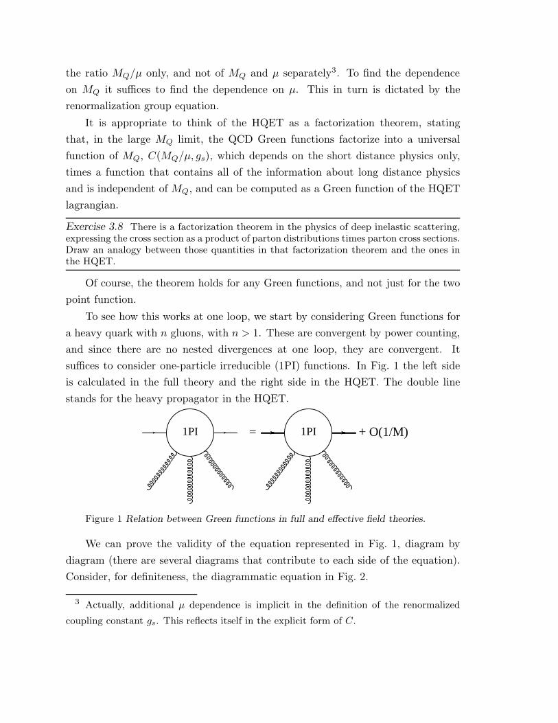
suffices to consider one-particle irreducible (1PI) functions. In Fig. 1 the left side
is calculated in the full theory and the right side in the HQET. The double line
stands for the heavy propagator in the HQET.
1PI 1PI= + O(1/M)
Figure 1 Relation between Green functions in full and effective field theories.
We can prove the validity of the equation represented in Fig. 1, diagram by
diagram (there are several diagrams that contribute to each side of the equation).
Consider, for definiteness, the diagrammatic equation in Fig. 2.
3 Actually, additional µ dependence is implicit in the definition of the renormalized
coupling constant gs. This reflects itself in the explicit form of C.
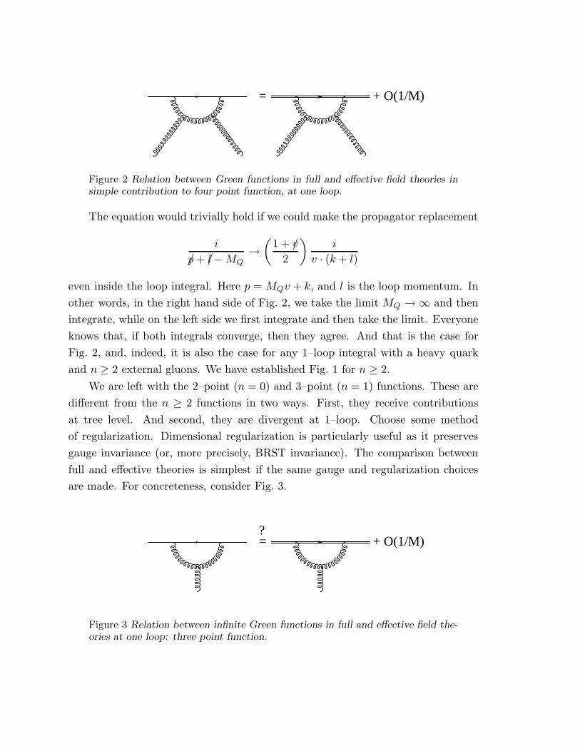
= + O(1/M)
Figure 2 Relation between Green functions in full and effective field theories insimple contribution to four point function, at one loop.
The equation would trivially hold if we could make the propagator replacement
i
/p+ /l −MQ→(
1 + v/
2
)i
v · (k + l)
even inside the loop integral. Here p = MQv + k, and l is the loop momentum. In
other words, in the right hand side of Fig. 2, we take the limit MQ →∞ and then
integrate, while on the left side we first integrate and then take the limit. Everyone
knows that, if both integrals converge, then they agree. And that is the case for
Fig. 2, and, indeed, it is also the case for any 1–loop integral with a heavy quark
and n ≥ 2 external gluons. We have established Fig. 1 for n ≥ 2.
We are left with the 2–point (n = 0) and 3–point (n = 1) functions. These are
different from the n ≥ 2 functions in two ways. First, they receive contributions
at tree level. And second, they are divergent at 1–loop. Choose some method
of regularization. Dimensional regularization is particularly useful as it preserves
gauge invariance (or, more precisely, BRST invariance). The comparison between
full and effective theories is simplest if the same gauge and regularization choices
are made. For concreteness, consider Fig. 3.
= + O(1/M)?
Figure 3 Relation between infinite Green functions in full and effective field the-ories at one loop: three point function.
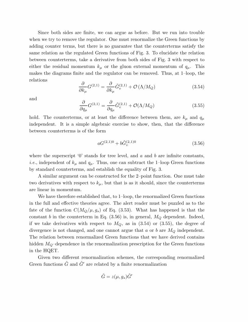
Since both sides are finite, we can argue as before. But we run into trouble
when we try to remove the regulator. One must renormalize the Green functions by
adding counter terms, but there is no guarantee that the counterterms satisfy the
same relation as the regulated Green functions of Fig. 3. To elucidate the relation
between counterterms, take a derivative from both sides of Fig. 3 with respect to
either the residual momentum kµ or the gluon external momentum of qµ. This
makes the diagrams finite and the regulator can be removed. Thus, at 1–loop, the
relations∂
∂kµG(2,1) =
∂
∂kµG(2,1)
v +O (Λ/MQ) (3.54)
and∂
∂qµG(2,1) =
∂
∂qµG(2,1)
v +O(Λ/MQ) (3.55)
hold. The counterterms, or at least the difference between them, are kµ and qµindependent. It is a simple algebraic exercise to show, then, that the difference
between counterterms is of the form
aG(2,1)0 + bG(2,1)0v (3.56)
where the superscript ‘0’ stands for tree level, and a and b are infinite constants,
i.e., independent of kµ and qµ. Thus, one can subtract the 1–loop Green functions
by standard counterterms, and establish the equality of Fig. 3.
A similar argument can be constructed for the 2–point function. One must take
two derivatives with respect to kµ, but that is as it should, since the counterterms
are linear in momentum.
We have therefore established that, to 1–loop, the renormalized Green functions
in the full and effective theories agree. The alert reader must be puzzled as to the
fate of the function C(MQ/µ, gs) of Eq. (3.53). What has happened is that the
constant b in the counterterm in Eq. (3.56) is, in general, MQ dependent. Indeed,
if we take derivatives with respect to MQ, as in (3.54) or (3.55), the degree of
divergence is not changed, and one cannot argue that a or b are MQ independent.
The relation between renormalized Green functions that we have derived contains
hidden MQ–dependence in the renormalization prescription for the Green functions
in the HQET.
Given two different renormalization schemes, the corresponding renormalized
Green functions G and G′ are related by a finite renormalization
G = z(µ, gs)G′
Choosing G to be the mass–independent subtracted Green function, and G′ the
one in our peculiar subtraction scheme, we have that the relation between full and
effective theories becomes
G(2,1)(p, q;µ) = C (MQ/µ, gs) G(2,1)v (k, q;µ) +O (Λ/MQ)
as advertised in Section 3.2. Here, C is nothing but this finite renormalization
z(µ, gs). That we can use the same function C for all Green functions can be
established by using the same wave functions renormalization prescription for gluons
in the full and effective theories. Otherwise, an additional factor of zn/2A would
have to be included in the relation between G(2,n) and G(2,n). This completes the
argument.
It is worth mentioning that the discussion above assumes the renormalizability,
preserving BRST invariance, of the effective theory. Although, to my knowledge,
this has not been established, there is no obvious reason to doubt that the standard
techniques apply in this case.
3.9. External Currents
We will often be interested in computing Green functions with an insertion of
a current. Consider, the current
JΓ = q ΓQ (3.57)
in the full theory, where Γ is some Dirac matrix, and q a light quark. In the effective
theory, this is replaced according to
JΓ(x)→ e−iMQv·xJΓ(x) , (3.58)
where
JΓ = q ΓQv , (3.59)
and it is understood that in JΓ the heavy quark is that of the HQET, satisfying,
in particular, v/Qv = Qv. The exponential factor in Eq. (3.58) reminds us to take
the large momentum out through the current, allowing us to keep the external
momentum of light quarks and gluons small. The relation between full and effective
theories takes the form of an approximate equation between Green functions —and
eventually amplitudes— of insertions of these currents:
GJΓ(p, p′; q;µ) = C(MQ/µ, gs)
1/2CΓ(MQ/µ, gs)Gv,JΓ(k, k′; q;µ) +O(Λ/MQ) ,
(3.60)
where p and p′ are the momenta of the heavy quark and the external current, k and
k′ the corresponding residual momenta, p = MQv+ k, p′ = MQv+ k′, and q stands
for the momenta of the light degrees of freedom. The factor C1/2CΓ accounts for
the logarithmic mass dependence, as explained earlier. We see that an additional
factor, namely, CΓ, is needed in this case to account for the different scaling behavior
of the currents in the full and effective theories. It is convenient to think of the
replacement of currents, not as given by Eq. (3.58), but rather by
JΓ(x)→ e−iMQv·xCΓ(MQ/µ, gs)JΓ(x) . (3.61)
In fact, Eq. (3.60), and therefore the replacement in Eq. (3.61), are not quite
correct. To reproduce the matrix elements of the current JΓ of Eq. (3.57), it is
necessary to sum over matrix elements of several different ‘currents’ in the effective
theory. The operator JΓ of Eq. (3.59) is just one of them. In addition, one may
have to introduce such operators as qv/ΓQv. The correct replacement is therefore
JΓ(x)→ e−iMQv·x∑
i
C(i)Γ (MQ/µ, gs)O(i)(x) . (3.62)
Here O(i)(x) is the collection of the operators of dimension 3 with appropriate
quantum numbers. The first operator in the sum, call it O(0), is there even at tree
level, and corresponds to the operator JΓ of Eq. (3.59).
Another case of interest is that of the insertion of a current of two heavy quarks
JΓ = Q′ΓQ . (3.63)
The replacement now is
JΓ(x)→ e−iMQv·x+iMQ′v′·x∑
i
C(i)Γ (
MQ
µ,MQ′
MQ, v·v′, gs)O(i)
Γ (x) . (3.64)
Again, O(i)(x) stands for the complete list of operators of dimension 3 in the effective
theory with the right quantum numbers. Also, the operator O(0) = Q′v′ΓQv appears
in the sum at tree level.
This deserves some explanation. The Green functions now include two heavy
quarks. The functions C connecting these full and effective Green functions will
now, in general, depend on both MQ and MQ′ . Moreover, we can not argue that C
are independent of the velocities v and v′. In fact, this was true of the simpler case
considered in Section 3.8; but there, C could only depend on vµ through v2 = 1. In
the case at hand there is an additional invariant on which C can depend, namely v·v′.The explicit functional dependence on MQ in the functions CΓ and CΓ can be
obtained from a study of their dependence on the renormalization point µ. For
clarity of presentation we neglect operator mixing for now. When necessary, this
can be incorporated without much difficulty. Taking a derivative d/dµ on both sides
of Eqs. (3.53) and (3.61), we find
µd
dµCΓ = (γ
Γ− γ
Γ)CΓ (3.65)
where γΓ
and γΓ
are the anomalous dimensions of the currents JΓ and JΓ in the
full and effective theories, respectively. Of particular interest are the cases Γ = γµ
and Γ = γµγ5. These correspond, in the full theory, to conserved and partially
conserved currents, and therefore the corresponding anomalous dimensions vanish,
giving
µdCΓ
dµ= −γ
ΓCΓ (Γ = γµ, γµγ5) . (3.66)
Before we solve this equation, we recall that
µd
dµ= µ
∂
∂µ+ β(gs)
∂
∂gs. (3.67)
Here β is the QCD β–function, with perturbative expansion
β(g)
g= −b0
g2
16π2+ b1
(g2
16π2
)2
+ . . . , (3.68)
and
b0 = 11− 2
3nf , (3.69)
where nf is the number of quarks in the theory. For our purposes, nf should not
include the heavy quark. This is explained in the famous paper by Appelquist and
Carrazone[22]; it simply reflects the fact that the logarithmic scaling of gs is not
affected by heavy quark loops, since these are suppressed by powers of MQ. Now,
the solution to (3.66) is standard:
CΓ(µ, gs) = exp
(−∫ gs
gs(µ0)
dg′γ
Γ(g′)
β(g′)
)CΓ(µ0, gs(µ0)) (3.70)
where gs is the running coupling constant defined by
µ′ dgs(µ′)
dµ′ = β(gs(µ′)) , gs(µ) = gs . (3.71)
Choosing µ0 = MQ, and restoring the dependence on MQ, we have then
CΓ(MQ/µ, gs) = exp
(−∫ gs(µ)
gs(MQ)
dg′γ
Γ(g′)
β(g′)
)CΓ(1, gs(MQ)) . (3.72)
Therefore, the problem of determining CΓ(MQ/µ, gs) breaks down into two
parts. One is the determination of the anomalous dimensions γΓ. The other is the
calculation of CΓ(1, gs(MQ)). Both can be done perturbatively, and CΓ(MQ/µ, gs)
can thus be computed, provided µ and MQ are large enough so that gs(µ) and
gs(MQ) are small. One finds, for example, that in leading order CΓ is Γ independent
and there is no mixing:
CΓ(MQ/µ, gs) =
(αs(MQ)
αs(µ)
)aI
, (3.73)
where αs ≡ g2s/4π, and[23–24] aI ≡ −c1/2b0 = −6/(33− 2nf ).
Exercise 3.9 Obtain an expression for CΓ analogous to that of Eq. (3.72) but withoutassuming that the anomalous dimension γΓ of Eq. (3.65) vanishes.
We now turn to the computation of the coefficient CΓ for the current of two
heavy quarks in Eq. (3.64). A new difficulty arises. Because CΓ depends on three
dimensionful quantities, namely the masses MQ and MQ′ , and the renormalization
point µ, its functional dependence is not determined from the renormalization group
equation (even if we neglect the implicit dependence of gs on µ). Two different
approximations have been developed to deal with this problem:
I) Treat the ratio MQ′/MQ as a dimensionless parameter, and study the de-
pendence of CΓ on MQ′/µ through the renormalization group[25]. This is just like
what was done for the heavy-light case, so we can transcribe the result:
CΓ
(MQ′
µ,MQ′
MQ, v·v′, gs
)≈exp
(−∫ gs(µ)
gs(MQ′ )
dg′γ
Γ(g′)
β(g′)
)CΓ
(1,MQ′
MQ, v·v′, gs(MQ′)
).
(3.74)
Again
CΓ
(1,MQ′
MQ, v·v′, gs(MQ′)
)= 1 +O(αs(MQ′)) . (3.75)
But, now, the correction of order αs(MQ′) is a function of MQ′/MQ. This method
has the advantage that the complete functional dependence on MQ′/MQ is retained,
order by order in αs(MQ′). Nevertheless, it fails to re–sum the leading–logs between
the scales MQ′ and MQ, i.e., it does not include the effects of running of the QCD
coupling constant between MQ and MQ′ . Therefore, this method is useful when
MQ′/MQ ∼ 1, or, equivalently, when (αs(MQ′)− αs(MQ))/αs(MQ)≪ 1.
II) Treat the ratio MQ′/MQ as small. Expand first in a HQET treating Q
as heavy and Q′ as light. The corrections are not just of order Λ/MQ but also
MQ′/MQ, but this is assumed to be small (even if much larger than Λ/MQ). Then
expand from this HQET, in powers of Λ/MQ′ , by constructing a new HQET where
both Q and Q′ are heavy[16]. The calculation of CΓ then proceeds in two steps.
The first gives a factor just like that of the heavy-light current, in (3.72)
exp
(−∫ gs(µ)
gs(MQ)
dg′γ
Γ(g′)
β(g′)
)CΓ(1, gs(MQ)) . (3.76)
The second factor is as in method I, above, but neglecting MQ′/MQ. Moreover, the
current JΓ is not conserved, so the anomalous dimension to be used is not −γΓ
but
γΓ−γ
Γ. Finally, we must make explicit the fact that in the first and second steps the
appropriate β-functions differ in the number of active quarks. We therefore label
the one in the second step β′ and the corresponding running coupling constant g′s.
The second factor is
exp
(∫ gs(µ)
gs(MQ′ )
dg′γ
Γ(g′)
β(g′)−∫ g′
s(µ)
g′
s(MQ′ )
dg′′γ
Γ(g′′)
β′(g′′)
)CΓ(1, 0, v·v′, gs(MQ′)) . (3.77)
Combining factors gives
CΓ
(MQ′
µ,MQ′
MQ, v·v′, gs
)≈ exp
(−∫ gs(MQ′ )
gs(MQ)
dg′γ
Γ(g′)
β(g′)−∫ g′
s(µ)
g′
s(MQ′ )
dg′′γ
Γ(g′′)
β′(g′′)
)
× CΓ(1, gs(MQ))CΓ(1, 0, v·v′, gs(MQ′)) .
(3.78)
The advantage of method II over method I is that it does include the effects
of running between MQ and MQ′ . The disadvantage is that it neglects powers of
MQ′/MQ. (Actually, the result can be improved by reincorporating the MQ′/MQ
dependence, as a power series expansion in this ratio).
For example, in method II eqn. (3.64) becomes, in leading order,[16]
cγµb→(αs(mb)
αs(mc)
)aI(α′
s(mc)
α′s(µ)
)aL
cv′ [(1 + κ)γµ + (λb − λc(v·v′))v/γµ]bv (3.79)
for Γ = γµ, and
cγµγ5b→(αs(mb)
αs(mc)
)aI(α′
s(mc)
α′s(µ)
)aL
cv′ [(1 + κ)γµγ5 − (λb + λc(v·v′))v/γµγ5]bv
(3.80)
for Γ = γµγ5, where
λb =αs(mb)
3π, λc(v·v′) =
2αs(mc)
3πr(v·v′) ,
aL(v·v′) =8
33− 2nf[v·v′r(v·v′)− 1] ,
r(x) ≡ 1√x2 − 1
ln(x+
√x2 − 1
),
(3.81)
and κ is of order αs but a subleading log.
Exercise 3.10 Why is the term involving κ in Eqs. (3.79) and (3.80) a subleading log,while those involving λb and λc are leading logs?
3.10. Form factors in order αs
The predicted relations between form factors, and normalizations at q2max, are
only approximate. Indeed, several approximations were made in obtaining those
results. Corrections that arise from subleading order in the 1/M expansion will be
considered in Chapter 4. Here we will discuss corrections of order αs.
As observed in Section 3.9, the vector and axial–vector currents of the full the-
ory, cΓb, match onto a linear combination of ‘currents’, i.e., dimension 3 operators,
in the effective theory. At one loop, the correspondence between vector and axial
currents in the full and effective theories is given by Eqs. (3.79) and (3.80). The
constant λb and the function λc arise only from 1-loop matching, and are scheme
independent. The constant κ receives contributions both from matching at 1-loop,
and from 2-loops anomalous dimensions. Leaving out the latter would give a mean-
ingless, scheme dependent, result. Although κ has been computed, it is interesting
to note that predictions can be made solely form the 1-loop matching computation.
Indeed, comparing Eqs. (3.45) with Eqs. (3.41), we see that at zeroth order in
αs(mb) or αs(mc) we have
a+ + a− = 0. (3.82)
Plugging Eq. (3.80) into Eq. (3.42) we see that, to order αs(mc) and αs(mb) there
is a computable correction to this combination of form factors, namely
a+ + a−a+
= −4mc
mb
[αs(mb)
3π+
2αs(mc)
3πr(v·v′)
](3.83)
The constant κ, although difficult to compute, does not change the relations be-
tween form factors since it simply rescales the leading order predictions in Eq. (3.45)
by the common factor of (1 + κ). It does, however, affect the predicted normaliza-
tion of form factors at q2max. Since at v′ = v the effective vector current is again
cv′γµbv, but rescaled by (1 + κ+ λb − λc(1)), the correction to Eq. (3.48) is
f±(q2max) = (1 + κ+ λb − λc(1))
(αs(mb)
αs(mc)
)aI(MD ±MB
2√MBMD
). (3.84)
We emphasize that retaining the constant κ in Eq. (3.84) is inconsistent, because
not all next to leading logs are included. For a calculation of the sub-leading logs,
including the constant κ, see Ref. [26].
4. 1/MQ
4.1. The Correcting Lagrangian
One of the main virtues of the HQET is that, in contrast to models of the
strongly bound hadrons, it lets us study systematically the corrections arising from
the approximations we have made. To be sure, we’ve made several approximations
already, even within the zeroth order expansion in Λ/MQ. For example, we have
computed the logarithmic dependence on MQ, i.e., the functions C(i)Γ and C
(i)Γ of
Eqs. (3.62) and (3.64), using perturbation theory. In this Section we turn to the
corrections of order Λ/MQ.
The HQET lagrangian was derived, in Section 3.2, by putting the heavy quark
almost on-shell and expanding in powers of the residual momentum, kµ, or light
quark or gluon momentum, qµ, over MQ, which we generally wrote as Λ/MQ. Let
us again derive the effective lagrangian, keeping track, this time, of the terms of
order Λ/MQ.
We will rederive L(v)eff , including 1/MQ corrections, working directly in configu-
ration space[27]. The heavy quark equation of motion is
(i/D −MQ)Q = 0 (4.1)
We can put the quark almost on shell by introducing the redefinition
Q = e−iMQv·xQv (4.2)
In terms of Qv, the equation of motion is
[i/D +MQ(v/− 1)]Qv = 0 (4.3)
If we separate the (1 + v/) and (1− v/) components of Qv, we see that, as expected,
the latter is very heavy and decouples in the infinite mass limit. To project out the
components,
Qv = Q(+)v + Q(−)
v (4.4)
where
Q(±)v =
(1± v/
2
)Qv , (4.5)
we multiply Eq. (4.3) by ( 1±v/2 ). Thus we have the equations
iv·DQ(+)v = −
(1 + v/
2
)i/DQ(−)
v (4.6)
and
iv·DQ(−)v + 2MQQ
(−)v =
(1− v/
2
)i/DQ(+)
v (4.7)
These equations can be solved self-consistently by assuming that Q(+)v is order
(MQ)0 while Q(−)v is order M−1
Q . A recursive solution follows. From Eq. (4.7)
Q(−)v =
1
2MQ
(1− v/
2
)i/DQ(+)
v − i v·D2MQ
Q(−)v (4.8)
Substituting into Eq. (4.6) and dropping terms of order 1/M2Q, we have
iv·DQ(+)v = −
(1 + v/
2
)i/D
1
2MQ
(1− v/
2
)i/DQ(+)
v (4.9)
The right hand side involves(
1 + v/
2
)/D
(1− v/
2
)/D
(1 + v/
2
)=
(1 + v/
2
)[D2 − (v·D)2 + 1
2gsσµνGµν
](1 + v/
2
)
(4.10)
where σµν = i2[γµ, γν] and Gµν = 1
igs[Dµ, Dν ] is the QCD field strength tensor.
This equation of motion is obtained from the lagrangian
L(v)eff = Qviv·DQv +
1
2MQQv
[D2 − (v·D)2 +
gs
2σµνGµν
]Qv (4.11)
Here I have reverted to the notation Qv for Q(+)v . How to include higher order
terms in the 1/MQ expansion into L(v)eff should be clear.
Exercise 4.1 Find the effective lagrangian describing a heavy scalar field to first orderin 1/M .
The 1/MQ term in L(v)eff is treated as small. If it is not, it does not make sense to
talk about a HQET in the first place. It is therefore appropriate to use perturbation
theory to compute its effects. In this perturbative expansion, the corrections of order
1/MQ to Green functions, and therefore to physical observables, are computed by
making a single insertion of the perturbation
∆L =1
2MQQv
[D2 − (v·D)2 +
gs
2σµνGµν
]Qv . (4.12)
The symmetries of the HQET, discussed at length in Sections 3.1 and 3.3, are
broken by ∆L. Under the SU(Nf )–flavor symmetry, ∆L transforms as a combi-
nation of the Adjoint and Singlet representations, while only the chromo-magnetic
moment operator
QvσµνGµνQv (4.13)
breaks the spin-SU(2) symmetry: it transforms as a 3 of spin–SU(2).
A single insertion of ∆L does include all orders in QCD, and it will often prove
difficult to make precise calculations of 1/MQ effects. Since ∆L is treated as a simple
insertion in Green functions, its treatment in the HQET is entirely analogous to
that of current operators of Section 3.9. There are coefficient functions that connect
the HQET results with the full theory. It is convenient to include them directly
into the effective lagrangian as[27,28,29]
∆L =1
2MQQv
[c1D
2 + c2(v·D)2 + 12c3gsσ
µνGµν
]Qv. (4.14)
Here
ci = ci(MQ/µ, gs) (4.15)
can be determined through the methods discussed extensively in Section 3.9. In
leading-log, one finds[27]
c1 = −1
c2 = 3
(αs(µ)
αs(MQ)
)−8/(33−2nf )
− 2
c3 = −(
αs(µ)
αs(MQ)
)−9/(33−2nf )
.
(4.16)
4.2. The Corrected Currents
Just as the lagrangian is corrected in order 1/MQ, any other operator is too. In
particular, the current operators studied in Section 3.9, are modified in this order.
At tree level, these corrections are given by the change of variables of last Section:
JΓ = qΓQ→ qΓe−iMQv·x[Qv +
1
2MQ
(1− v/
2
)i/DQv
]. (4.17)
Beyond tree level, this sum of two terms has to be replaced by a more general
sum over operators of the right dimensions and quantum numbers. The replacement
is
JΓ → e−iMQv·x∑
i
C(i)Γ qΓiQv +
1
2MQ
∑
j
D(j)Γ Oj
(4.18)
where Oj are operators of dimension 4 that include, for example, the operators
qΓi/DQv , qΓi(v·D)Qv , qv/Γi/DQv . (4.19)
A complete set of operators, and the corresponding coefficients, D(i)Γ , for the cases
Γ = γµ and Γ = γµγ5, can be found in Refs. [28,30] in the leading-log approximation.
The case of two heavy currents is similar. A straightforward calculation gives
JΓ = Q′ΓQ→e−iMQv·x+iMQ′v′·x[Q′v′ΓQv
+1
2MQQ′
v′Γ
(1− v/
2
)i/DQv +
1
2MQ′
Q′v′i←−/D
(1− v/
2
)ΓQv
] (4.20)
Again, beyond tree level we must replace this expression by a more general sum
over operators of dimension four,
JΓ → e−iMQv·x+iMQ′v′·x[∑
i
C(i)Γ Q′
v′ΓiQv +1
2MQ
∑
j
D(j)Γ Oj
+1
2MQ′
∑
j
D′(j)Γ Oj
(4.21)
It is worth pointing out that, in the computation of the coefficient functions
D(j)Γ , D
(j)Γ and D
′(j)Γ , there is a contribution from the term of order (1/MQ)0. In
computing the coefficient functions to order 1/MQ one must not forget graphs with
one insertion of the zeroth order term in the current and one insertion of the first
order term in the HQET lagrangian.
4.3. Corrections of order mc/mb
In the case of semileptonic decays of a beauty hadron to charmed hadron,
we introduced earlier an approximation method (“Method II” in Section 3.8) in
which mc/mb was treated as a small parameter. Now, mc/mb ∼ 1/3 and you may
justifiably worry that this is not a good expansion parameter. We will see in this
Section that the corrections are actually of the order of αs/π(mc/mb) and therefore
small. Moreover, they are explicitly calculable.
The strategy is[28] to look at those corrections of order 1/mb which may be
accompanied by a factor of mc. In the first step of the approximation scheme we
construct a HQET for the b-quark, treating the c-quark as light. We must, of course,
keep terms of order 1/mb in this first step. The second step is to go over to a HQET
in which the mc-quark is also heavy. For now, we care only about terms in this
HQET that have positive powers of mc.
In the first step, the hadronic current cΓb, with Γ = γµ or Γ = γµγ5, is replaced
according to Eq. (4.18). The question is, which terms in Eq. (4.18) can give factors
of mc when we replace the c-quark by a HQET quark, cv′ . Recall that, once we
complete the second step, all of the mc dependence is explicit. The answer is that
any operators in Eq. (4.18) which have a derivative acting on the c-quark will give a
factor of mc. From Eq. (4.2) we see that a derivative i∂µ acting on the charm quark
becomes, in the effective theory, the operation mcv′µ + i∂µ. So the prescription is
simple: take JΓ in Eq. (4.18) and replace
i∂µ → mcv′µ (4.22)
in those terms where i∂µ is acting on the charm quark.
For example, if the operator
1
mbc i←−/D Γbv (4.23)
is generated at some order in the loop expansion, it gives an operator
−mc
mbcv′v/′Γbv = −mc
mbcv′Γbv (4.24)
after step two is completed.
It is really interesting to note that the resulting correction does not introduce
any new unknown form factors. For example, the matrix element of (4.24) between
a B and a D is given by Eq. (3.42) only with an additional factor of −mc/mb in
front.
The calculation described here has been performed in the leading-log approxi-
mation in Ref. [28]. The correction to the vector current is
∆Vµ =mc
mbcv′(a1γµ + a2vµ + a3v
′µ)bv (4.25)
where the coefficients ai = ai(µ), written in terms of
z =αs(mc)
αs(mb)(4.26)
are
a1 =5
9(v·v′ − 1)− 1
18z−
625 +
2v·v′ + 12
27z−
325 − 34v·v′ − 9
54z
625 − 8
25v·v′z 6
25 ln z
a2 =5
9(1− 2v·v′)− 13
9z−
625 − 44v·v′ − 6
27z−
325 − 14v·v′ − 18
27z
625
a3 =15
9− 2
3z−
325 − z 6
25
(4.27)
In particular, this gives a contribution to the form factor, at v = v′, of
mc
mb(a1 + a2 + a3)|v·v′=1 ≃ .07 (4.28)
This is not negligible! It is reassuring that this type of corrections can be extracted
explicitly. On the other hand, it should be remembered that both corrections of
order (mc/mb)2 and of subleading-log order can still be considerable and should be,
but have not been, computed.
4.4. Corrections of order Λ/mc and Λ/mb.
Corrections to the form factors for semileptonic decays of B’s and Λb’s that arise
from the terms of order 1/mc in the effective lagrangian Eq. (4.11) and the currents
Eqs. (4.18) and (4.21) are, in principle, as large or larger than those considered in the
previous Section. It is a welcome surprise that the corrections to the combination
of form factors that contribute to the semileptonic decay vanish at the endpoint
v·v′ = 1. Thus, the predicted normalization of form factors persists, although, as
we will see, not so the relations between form factors.
The decay[31] Λb → Λceν is simpler to analyze than the decays[32] B → Deν
and B → D∗eν. Moreover, it turns out that for the baryonic decay some relations
between form factors survive at this order. For these reasons, we will present here
the baryonic case. We will briefly return to the decay of the meson at the end of
this section, where we will describe the result.
There are two types of corrections to consider[31], coming from either the mod-
ified lagrangian of from the modified current. We start by considering the former.
The c1 and c2 terms in the effective lagrangian (4.14) transform trivially under the
spin symmetry, contributing to the form factors in the same proportion as the lead-
ing term in Eq. (3.49). This effectively renormalizes the function ζ but does not
affect relations between form factors.
Moreover, the normalization at the symmetry point v·v′ = 1 is not affected.
This is a straightforward application of the Ademollo-Gatto theorem. If jµ is a
symmetry generating current of a hamiltonian H0, then corrections to the matrix
element of the current, at zero momentum, from a symmetry-breaking perturbation
to the hamiltonian, ǫH1, are of order ǫ2. In the case at hand the Ademollo-Gatto
theorem implies that corrections to the normalization of ζ at the symmetry point
are of order (1/mc)2.
The chromomagnetic moment operator in the lagrangian (4.14) does not give a
contribution at all. The spin symmetries imply
〈Λc(v′, s′)|T
∫d4x (cv′σµνGµνcv′)(x)(cv′Γbv)(0)|Λb(v, s)〉
= ζµν(v, v′)u(s′)(v′)σµν
(1 + v/
2
)Γu(s)(v).
(4.29)
The function ζµν must be an antisymmetric tensor and must therefore be propor-
tional to v′µvν − v′νvµ. But
(1 + v/′
2
)σµν
(1 + v/′
2
)v′µ = 0. (4.30)
This, we see, is an enormous simplification. There is no analogous simple reason
for the matrix element of the chromomagnetic moment operator to vanish in the
case of a meson transition. The chromomagnetic matrix element gives, in that case,
uncalculable corrections to the relations between form factors.
We turn next to the contribution from the modification to the current. We
need the matrix element of the local operators of order 1/mc in Eq. (4.21). These
operators are all constructed of one derivative acting on either heavy quark in the
quark bilinear. Consider the matrix element
〈Λc(v′, s′)|cv′i
←−DµΓbv|Λb(v, s)〉 = u(s′)(v′)Γu(s)(v)[Avµ +Bv′µ], (4.31)
where the form of the right hand side follows again from the spin symmetries. The
form factors A and B are not independent. Rather, they are given in terms of ζ.
To see this, note that, contracting with v′µ and using the equations of motion,
B = −v·v′A. (4.32)
Also, if the mass of the l = 1/2 state in the effective theory is Λ, then
〈Λc(v′, s′)|i∂µ(cv′Γbv)|Λb(v, s)〉 = Λ(vµ − v′µ)ζ(v·v′)u(s′)(v′)Γu(s)(v). (4.33)
Contracting with vµ, using the equations of motion and Eq. (4.32) we have
A(1− (v·v′)2) = Λ(1− v·v′)ζ (4.34)
Therefore, the matrix element of interest is
〈Λc(v′, s′)|cv′i
←−/D Γbv|Λb(r, s)〉 = Λζ(v·v′)vν − (v·v′)v′ν
1 + v·v′ u(s′)(v′)γνΓu(s)(v) (4.35)
where Γ = γµ or γµγ5. Putting it all together, using the leading log expression for
the coefficients D(j)Γ in the current of Eq. (4.21), one finds
F1 = G1
[1 +
Λ
mc
(1
1 + v·v′)]
F2 = G2 = −G1Λ
mc
(1
1 + v·v′)
F3 = G3 = 0
(4.36)
Moreover,
G1(1) =
(αs(mb)
αs(mc)
)aI
(4.37)
as before. Up to an unknown constant, Λ, there are still five relations among six
form factors. We can estimate Λ by writing Λ = MΛc− mc = (MΛc
− MD) +
(MD − mc). If the ‘constituent’ quark mass in the D meson is ≃ 300MeV , then
Λ ≃ 700MeV . With this, we can estimate the next order corrections to be of the
order of(Λ/2mc
)2 ∼ 5%. There are, of course, additional computable corrections,
of order Λ/2mb and αs(mc)/π(Λ/2mc
).[33]
The result of 1/mc corrections to the mesonic transitions is quite different.
There both the matrix elements of the correction to the current and of the time order
product with the chromo-magnetic moment operator lead to new form factors. The
result is that there are incalculable corrections, of order Λ/2mc, to all the leading
order relations between form factors. Even if Λ is smaller in this case, presumably
Λ ∼ 300MeV, these corrections may be large, say 10%–20%. Remarkably, at the
symmetry point, v′·v = 1, there are no corrections of order Λ/2mc to the leading
order predictions. Thus, one may still extract the mixing angle |Vcb| with high
precision from measurements at the end of the spectrum of the semileptonic decay
rates for B → Deν and B → D∗eν.
5. Inclusive Semileptonic B-Meson Decays.
Well before the development of HQETs, it was commonly held that the inclusive
rate of decay of a heavy meson should be well approximated by the decay rate of
the heavy quark. Intuitively, the heavy quark just sits at rest (in the rest frame
of the meson) surrounded by ‘brown muck’ for which it acts as a static source of
color. When the heavy quark decays, the complications of strong interactions come
in, dictating how the rate is divided up between exclusive channels, but the sum
total must be the quark’s rate of decay.
With the advent of HQET and HQ symmetries one may prove the validity
of this assertion. Moreover, and more importantly, this is done by setting up an
expansion for the decay rate in inverse powers of the heavy mass. With a systematic
expansion one may investigate the accuracy of the result for the not-really-so-heavy
D and B mesons.
5.1. Kinematics.
The decay rate is
dΓ =κ
2M
∑
X
|〈X |jµ|B〉ℓµ|2dΦX (5.1)
where jµ is the hadronic ∆B = −1 current,
dΦX ∝ δ(4)(P − pX − pe − pν) Πid3pi
2Ei(5.2)
is the phase space for final states and
ℓµ = v(pν)γµ(1− γ5)u(pe) (5.3)
is the lepton current. The factor κ includes the coupling constants G2F |Vqb|2.
All of the interesting dynamics is in the hadronic tensor
hµν =∑
X
(2π)3δ(4)(P − px − q)〈B|j†ν(0)|X〉〈X |jµ(0)|B〉 (5.4)
where the sum symbol includes the integral over phase space for the final state X .
We will investigate the properties of the hadronic tensor hµν indirectly, by
studying the related tensor
Tµν = i
∫d4x e−iq·x〈B(p)|T (j†ν(x)jµ(0))|B〉 (5.5)
Both tensors can be written in terms of Lorentz invariant form factors, thus:
hµν = gµνh1 + pµpνh2 + · · · (5.6a)
Tµν = gµνT1 + pµpνT2 + · · · (5.6b)
Exercise 5.1 I have intentionally left the list of form factors incomplete. The ellipsis inEqs. (5.6) stand for a finite number of terms. Ennumerate them. There is one term thatcan be eliminated by the requirement of time reversal invariance of the strong interactions.Which one is it?
The form factors Ti are more amenable to theoretical investigations because
Tµν is a Green function. The hi form factors can be obtained from these by cutting:
hi =1
πImTi for p · q < m2
B (5.7)
Exercise 5.2 To see this,(i) Separate the integral in Eq. (5.5) into x0 > 0 and x0 < 0 parts. Insert a complete set
of states between the two currents, and make the dependence on x explicit.(ii) Carry out the integrations, using, eg,
∫d4x θ(x0)ei(P−pX−q)·x = (2π)3δ( ~P − ~pX − ~q)
i
P 0 − p0X − q0 + iǫ
and use the standard identity
1
z ± iǫ= PP
1
z∓ iπδ(z) ,
where PP stands for the principal part, to separate “imaginary” from “real” parts(these are in quotation marks because by them I just mean the parts that come fromthe PP terms and from the δ term, respectively).
(iii) In the “imaginary” part you will recognize one term is just hµν . Write out explicitlythe other term in the “imaginary” part and show that it vanishes if P ·q < mB . (Hint:What is the lowest mass of the intermediate state X?).
(iv) Complete the proof by relating form factors and taking, where appropriate, the realor imaginary parts.
5.2. The Analytic Structure of The Hadronic Green Function
The hadronic form factors Ti and hi are Lorentz invariant functions of the
momenta P and q. There are only two invariant variables, namely Q ≡√q2/m2
B
and z ≡ P · q/m2B . Here and throughout a hat on a dimensionful quantity means
taking out the dimensions by apropriate powers of mB . We will study the behaviour
of Tµν for fixed Q2 as a function of z. This variable is of interest because 1 − zmeasures how far one is from the resonant region. To see this, consider any final
state X contributing to the inclusive decay, so q = P−pX . Then z = 1−P ·pX/m2B ,
or, in the rest frame of the decaying meson, 1 − z = EX/mB . Only states with
small energy contribute to the region of z ≈ 1, and only single resonances contribute
when z is large enough.
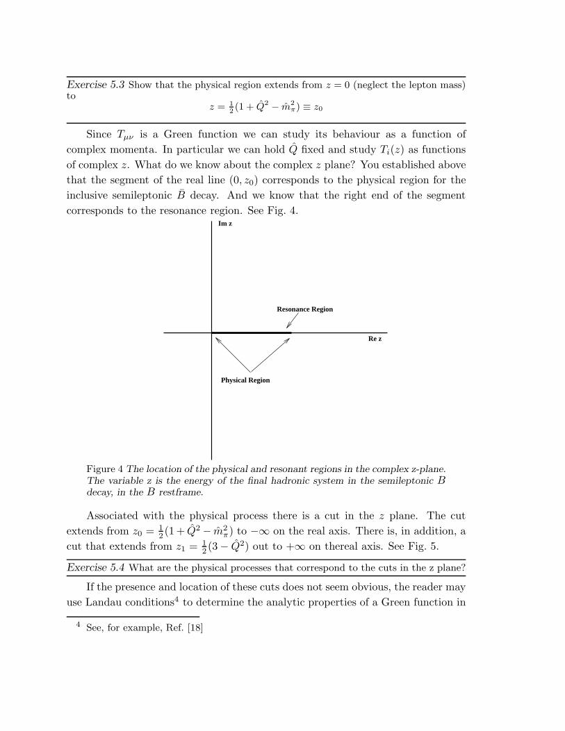
Exercise 5.3 Show that the physical region extends from z = 0 (neglect the lepton mass)to
z = 12(1 + Q2 − m2
π) ≡ z0
Since Tµν is a Green function we can study its behaviour as a function of
complex momenta. In particular we can hold Q fixed and study Ti(z) as functions
of complex z. What do we know about the complex z plane? You established above
that the segment of the real line (0, z0) corresponds to the physical region for the
inclusive semileptonic B decay. And we know that the right end of the segment
corresponds to the resonance region. See Fig. 4.
Resonance Region
Physical Region
Re z
Im z
Figure 4 The location of the physical and resonant regions in the complex z-plane.The variable z is the energy of the final hadronic system in the semileptonic Bdecay, in the B restframe.
Associated with the physical process there is a cut in the z plane. The cut
extends from z0 = 12(1 + Q2 − m2
π) to −∞ on the real axis. There is, in addition, a
cut that extends from z1 = 12(3− Q2) out to +∞ on thereal axis. See Fig. 5.
Exercise 5.4 What are the physical processes that correspond to the cuts in the z plane?
If the presence and location of these cuts does not seem obvious, the reader may
use Landau conditions4 to determine the analytic properties of a Green function in
4 See, for example, Ref. [18]
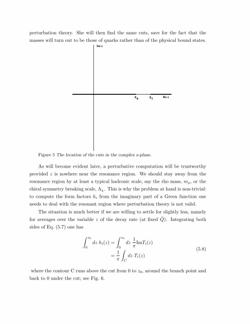
perturbation theory. She will then find the same cuts, save for the fact that the
masses will turn out to be those of quarks rather than of the physical bound states.
z1z0 Re z
Im z
Figure 5 The location of the cuts in the complex z-plane.
As will become evident later, a perturbative computation will be trustworthy
provided z is nowhere near the resonance region. We should stay away from the
resonance region by at least a typical hadronic scale, say the rho mass, mρ, or the
chiral symmetry breaking scale, Λχ. This is why the problem at hand is non-trivial:
to compute the form factors hi from the imaginary part of a Green function one
needs to deal with the resonant region where perturbation theory is not valid.
The situation is much better if we are willing to settle for slightly less, namely
for averages over the variable z of the decay rate (at fixed Q). Integrating both
sides of Eq. (5.7) one has
∫ z0
0
dz hi(z) =
∫ z0
0
dz1
πImTi(z)
=1
π
∫
C
dz Ti(z)
(5.8)
where the contour C runs above the cut from 0 to z0, around the branch point and
back to 0 under the cut; see Fig. 6.
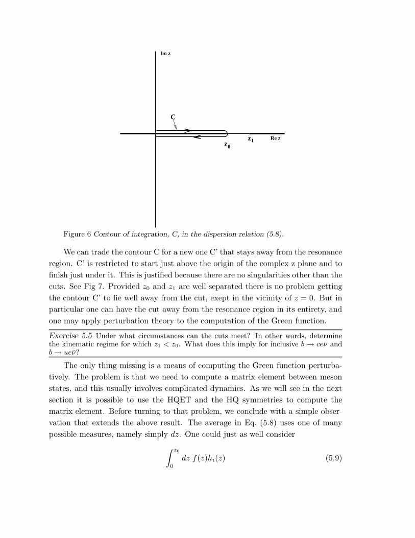
z1 Re z
Im z
C
z0
Figure 6 Contour of integration, C, in the dispersion relation (5.8).
We can trade the contour C for a new one C’ that stays away from the resonance
region. C’ is restricted to start just above the origin of the complex z plane and to
finish just under it. This is justified because there are no singularities other than the
cuts. See Fig 7. Provided z0 and z1 are well separated there is no problem getting
the contour C’ to lie well away from the cut, exept in the vicinity of z = 0. But in
particular one can have the cut away from the resonance region in its entirety, and
one may apply perturbation theory to the computation of the Green function.
Exercise 5.5 Under what circumstances can the cuts meet? In other words, determinethe kinematic regime for which z1 < z0. What does this imply for inclusive b → ceν andb→ ueν?
The only thing missing is a means of computing the Green function perturba-
tively. The problem is that we need to compute a matrix element between meson
states, and this usually involves complicated dynamics. As we will see in the next
section it is possible to use the HQET and the HQ symmetries to compute the
matrix element. Before turning to that problem, we conclude with a simple obser-
vation that extends the above result. The average in Eq. (5.8) uses one of many
possible measures, namely simply dz. One could just as well consider
∫ z0
0
dz f(z)hi(z) (5.9)
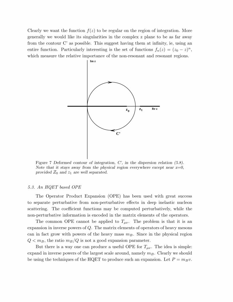
Clearly we want the function f(z) to be regular on the region of integration. More
generally we would like its singularities in the complex z plane to be as far away
from the contour C’ as possible. This suggest having them at infinity, ie, using an
entire function. Particularly interesting is the set of functions fn(z) = (z0 − z)n,
which measure the relative importance of the non-resonant and resonant regions.
z1z0Re z
Im z
C’
Figure 7 Deformed contour of integration, C’, in the dispersion relation (5.8).Note that it stays away from the physical region everywhere except near z=0,provided Z0 and z1 are well separated.
5.3. An HQET based OPE
The Operator Product Expansion (OPE) has been used with great success
to separate perturbative from non-perturbative effects in deep inelastic nucleon
scattering. The coefficient functions may be computed perturbatively, while the
non-perturbative information is encoded in the matrix elements of the operators.
The common OPE cannot be applied to Tµν . The problem is that it is an
expansion in inverse powers of Q. The matrix elements of operators of heavy mesons
can in fact grow with powers of the heavy mass mB . Since in the physical region
Q < mB , the ratio mB/Q is not a good expansion parameter.
But there is a way one can produce a useful OPE for Tµν . The idea is simple:
expand in inverse powers of the largest scale around, namely mB . Clearly we should
be using the techniques of the HQET to produce such an expansion. Let P = mBv.
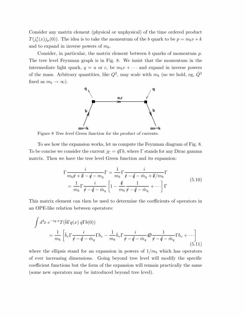
Consider any matrix element (physical or unphysical) of the time ordered product
T (j†ν(x)jµ(0)). The idea is to take the momentum of the b quark to be p = mbv+k
and to expand in inverse powers of mb.
Consider, in particular, the matrix element between b quarks of momentum p.
The tree level Feynman graph is in Fig. 8. We insist that the momentum in the
intermediate light quark, q = u or c, be mbv + · · · and expand in inverse powers
of the mass. Arbitrary quantities, like Q2, may scale with mb (so we hold, eg, Q2
fixed as mb →∞).
mv+k
q q
mv+k
b b
u,c
Figure 8 Tree level Green function for the product of currents.
To see how the expansion works, let us compute the Feynman diagram of Fig. 8.
To be concise we consider the current jΓ = qΓb, where Γ stands for any Dirac gamma
matrix. Then we have the tree level Green function and its expansion:
Γi
mbv/+ /k − /q −mqΓ =
1
mbΓ
i
v/− /q − mq + /k/mbΓ
=1
mbΓ
i
v/− /q − mq
[1− /k
mb
1
v/− /q − mq+ · · ·
]Γ
(5.10)
This matrix element can then be used to determine the coefficients of operators in
an OPE-like relation between operators:
∫d4x e−iq·xT (bΓq(x) qΓb(0))
=1
mb
[bvΓ
i
v/− /q − mqΓbv −
1
mbbvΓ
i
v/− /q − mqi/D
1
v/− /q − mqΓbv + · · ·
]
(5.11)
where the ellipsis stand for an expansion in powers of 1/mb which has operators
of ever increasing dimensions. Going beyond tree level will modify the specific
coefficient functions but the form of the expansion will remain practically the same
(some new operators may be introduced beyond tree level).
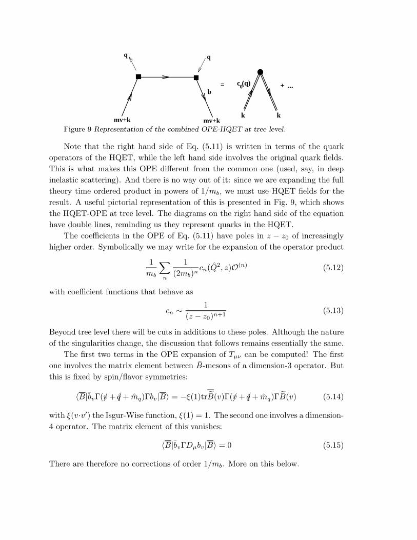
kk
0c (q)= + ...
mv+k
q q
mv+k
b
Figure 9 Representation of the combined OPE-HQET at tree level.
Note that the right hand side of Eq. (5.11) is written in terms of the quark
operators of the HQET, while the left hand side involves the original quark fields.
This is what makes this OPE different from the common one (used, say, in deep
inelastic scattering). And there is no way out of it: since we are expanding the full
theory time ordered product in powers of 1/mb, we must use HQET fields for the
result. A useful pictorial representation of this is presented in Fig. 9, which shows
the HQET-OPE at tree level. The diagrams on the right hand side of the equation
have double lines, reminding us they represent quarks in the HQET.
The coefficients in the OPE of Eq. (5.11) have poles in z − z0 of increasingly
higher order. Symbolically we may write for the expansion of the operator product
1
mb
∑
n
1
(2mb)ncn(Q2, z)O(n) (5.12)
with coefficient functions that behave as
cn ∼1
(z − z0)n+1(5.13)
Beyond tree level there will be cuts in additions to these poles. Although the nature
of the singularities change, the discussion that follows remains essentially the same.
The first two terms in the OPE expansion of Tµν can be computed! The first
one involves the matrix element between B-mesons of a dimension-3 operator. But
this is fixed by spin/flavor symmetries:
〈B|bvΓ(v/+ /q + mq)Γbv|B〉 = −ξ(1)trB(v)Γ(v/+ /q + mq)ΓB(v) (5.14)
with ξ(v·v′) the Isgur-Wise function, ξ(1) = 1. The second one involves a dimension-
4 operator. The matrix element of this vanishes:
〈B|bvΓDµbv|B〉 = 0 (5.15)
There are therefore no corrections of order 1/mb. More on this below.
Exercise 5.6 Prove Eq. (5.15). Hint: Consult section 4.4.
We see that one can compute the rate for inclusive semileptonic B decay. With
the tree level coefficient functions just computed, the matrix elements in Eqs. (5.14)
and (5.15), and neglecting higher order terms in 1/mb, one obtains for the decay
rate the same result as if computing the decay rate of a free b quark!
Exercise 5.7 Prove this assertion. In fact, we can do even better because we need notintegrate over Q2. Prove that the moments
∫ z0
0
dz (z0 − z)n dΓ(B → Xeν)
dz dQ2
are the same as for the free quark decay. This is an important exercise. You will haveto put together all the pieces of the argument discussed above, and then more.
The deviations from the free decay rate are parameterized by the matrix ele-
ments of the operators of dimension 5 and higher. In this sense we have managed
to separate long from short distance effects.
Note that for z on the real axis, the expansion breaks down as z → z0. More
precisely, in this limit the coefficients cn of Eq. (5.12) grow arbitrarily large. This
is in accord with the statement we had made previously that the perturbative
calculation of the Green function breaks down in the resonant region, z ∼ z0.A physically interesting choice of the measure f in Eq. (5.9) is f1 = z − z0,
because it measures the deviation from the free quark result. The quantity m2bf1(v ·
q/mb) is the invariant mass-squared of the hadronic final state minus m2q . If the
final state quark produced by the b decay is on its mass shell, then f1 = 0.
Exercise 5.8 Prove that with f1 = z − z0 the contribution from the parton model tothe average in Eq. (5.9) vanishes. Discuss corrections to this result arising from thenonperturbative terms and from the perturbative corrections to the coefficients in theexpansion of Eq. (5.12).
Exercise 5.9 |Vub| is determined from a measurement of inclusive charmless semileptonicB decay. Since Vub| ≪ |Vcb|, the rate for B → Xeν is dominated by the decay into charm.Short of reconstructing the hadronic state X, one is forced to consider the spectrum ofelectron energies, Ee. Find the maximum electron energies, Ec,max
e and Eu,maxe , in the
decay into charm and charmless final states, respectively. What does the region Ec,maxe <
Ee < Eu,maxe , correspond to in terms of our variables z and Q?
6. Chiral Lagrangian with Heavy Mesons
6.1. Generalities
Chiral symmetry and soft pion theorems have been used in particle physics for
several decades now with great success. The most efficient way of extracting infor-
mation from chiral symmetry is by writing a phenomenological lagrangian for pions
that incorporates both the explicitly realized vector symmetry and the non-linearly
realized spontaneously broken axial symmetry.[34] Theorems that simultaneously
use heavy quark symmetries and chiral symmetries are most expediently written by
means of a phenomenological lagrangian for pions and heavy mesons that incorpo-
rates these symmetries.[35,36]
In the limit mb →∞, the B and the B∗
mesons are degenerate, and to imple-
ment the heavy quark symmetries it is convenient to assemble them into a “super-
field” Ha(v):
Ha(v) =1 + v/
2
[B
∗µ
a γµ −Baγ5]. (6.1)
Here vµ is the fixed four-velocity of the heavy meson, and a is a flavor SU(3)
index corresponding to the light antiquark. Because we have absorbed mass factors√
2mB into the fields, they have dimension 3/2; to recover the correct relativistic
normalization, we will multiply amplitudes by√
2mB for each external B or B∗
meson.
The chiral lagrangian contains both heavy meson superfields and pseudogold-
stone bosons, coupled together in an SU(3)L×SU(3)R invariant way. The matrix of
pseudogoldstone bosons appears in the usual exponentiated form ξ = exp(iM/f),
where
M =
1√2π0 + 1√
6η π+ K+
π− − 1√2π0 + 1√
6η K0
K− K0 −
√23η
, (6.2)
and f is the meson decay constant. The bosons couple to the heavy fields through
the covariant derivative and axial vector field,
Dµab = δab∂
µ + V µab = δab∂
µ + 12
(ξ†∂µξ + ξ∂µξ†
)ab,
Aµab =
i
2
(ξ†∂µξ − ξ∂µξ†
)ab
= − 1
f∂µMab +O(M3) .
Lower case roman indices correspond to flavor SU(3). Under chiral SU(3)L ×SU(3)R, the pseudogoldstone bosons and heavy meson fields transform as
ξ → LξU† = UξR†
Aµ → UAµU†
H → HU †
(DµH)→ (DµH)U†
where the matrix U is a nonlinear function of the pseudogoldstone boson matrix
M, implicitly defined by the transformation law for ξ. Then Σ = ξ2transforms as
follows:
Σ→ LΣR† .
The effective lagrangian is an expansion in derivatives and in inverse powers of
the heavy quark mass. The kinetic energy terms take the form
Lkin =1
8f2 ∂µΣab ∂µΣ†
ba −Tr[Ha(v)iv ·DbaHb(v)
].
Here the trace is in the space of 4 × 4 Dirac matrices that define the “superfields”
Ha(v) in Eq. (6.1). The leading interaction term is of dimension four,
Lint = gTr[Ha(v)Hb(v)A/baγ5
], (6.3)
where g is an unknown parameter, of order one in the constituent quark model.
The analogous term in the charm system is responsible for the decay D∗ → Dπ.
Expanding the term in the lagrangian in (6.3) to linear order in the Goldstone
Boson fields, M, we find the explicit forms for the D∗DM and D∗D∗M couplings
[(−2g
f
)D∗ν∂µMD† + h.c.
]+
(2gi
f
)ǫµνλκD
∗µ∂νMD∗λvκ . (6.4)
Using this one can compute the partial width
Γ(D∗+ → D0π+) =g2
6πf2|~pπ|3
Γ(D∗+ → D+π0) =g2
12πf2|~pπ|3
The ACCMOR collaboration has reported an upper limit of 131 KeV on the
D∗ width.[37] The branching fractions for D∗+ → D0π+ and D∗+ → D+π0 are
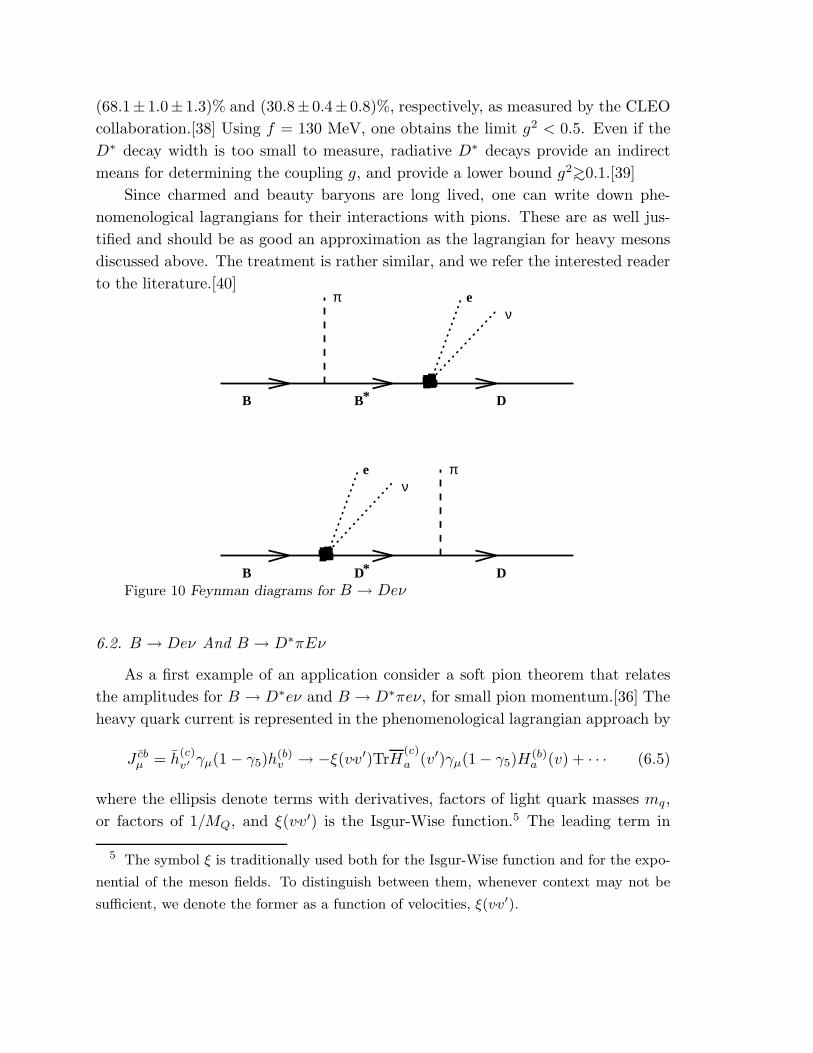
(68.1± 1.0± 1.3)% and (30.8± 0.4± 0.8)%, respectively, as measured by the CLEO
collaboration.[38] Using f = 130 MeV, one obtains the limit g2 < 0.5. Even if the
D∗ decay width is too small to measure, radiative D∗ decays provide an indirect
means for determining the coupling g, and provide a lower bound g2>∼0.1.[39]
Since charmed and beauty baryons are long lived, one can write down phe-
nomenological lagrangians for their interactions with pions. These are as well jus-
tified and should be as good an approximation as the lagrangian for heavy mesons
discussed above. The treatment is rather similar, and we refer the interested reader
to the literature.[40]
* DB
π
D
νe
ν
* DB
π
B
e
Figure 10 Feynman diagrams for B → Deν
6.2. B → Deν And B → D∗πEν
As a first example of an application consider a soft pion theorem that relates
the amplitudes for B → D∗eν and B → D∗πeν, for small pion momentum.[36] The
heavy quark current is represented in the phenomenological lagrangian approach by
J cbµ = h
(c)v′ γµ(1− γ5)h
(b)v → −ξ(v·v′)TrH
(c)
a (v′)γµ(1− γ5)H(b)a (v) + · · · (6.5)
where the ellipsis denote terms with derivatives, factors of light quark masses mq,
or factors of 1/MQ, and ξ(v·v′) is the Isgur-Wise function.5 The leading term in
5 The symbol ξ is traditionally used both for the Isgur-Wise function and for the expo-
nential of the meson fields. To distinguish between them, whenever context may not be
sufficient, we denote the former as a function of velocities, ξ(v·v′).
Eq. (6.5) is independent of the pion field. Therefore, it is pole diagrams that
dominate the amplitude for semileptonic B → Dπ and B → D∗π transitions; see
Fig. 10. These pole diagrams are calculable in this approach, and are determined
by the Isgur-Wise function and the coupling g.
A straightforward calculation gives[36]
〈D(v′)πa(q)|J cbµ |B(v)〉 = iu(B)∗ 1
2τau(D)
√MBMD
g
fξ(v·v′)
×
1
v·q [iǫµνλκqνv′λvκ + q · (v + v′)vµ − (1 + v·v′)qµ
− 1
v′·q [iǫµνλκqνv′λvκ + q · (v + v′)v′µ − (1 + v·v′)qµ
where u(M) stands for the isospin wavefunction of mesonM . A similar but lengthier
expression is found for B → D∗πeν. Even if the coupling g is close to its upper
limit, this expression makes a small contribution to the inclusive semileptonic rate.
6.3. Violations To Chiral Symmetry
Phenomenological lagrangians are particularly well suited to explore devia-
tions from symmetry predictions. We begin by introducing symmetry break-
ing terms into the phenomenological lagrangian. The light quark mass matrix
mq = diag(mu, md, ms) parametrizes the violations to flavor SU(3)V . To linear
order in mq and lowest order in the derivative expansion, the correction to the
phenomenological lagrangian is
∆L = λ0
[mqΣ +mqΣ
†]aa
+ λ1TrH(Q)a
H(Q)b
[ξmqξ + ξ†mqξ
†]ba
+ λ′1TrH(Q)a
H(Q)a
[mqΣ +mqΣ
†]bb (6.6)
The coefficients λ0, λ1 and λ′1 are fixed by non-perturbative strong interaction
effects, but may be determined phenomenologically. We postpone consideration of
mass relations obtained from this lagrangian until we have introduced heavy quark
spin symmetry breaking terms into the lagrangian too.
Exercise 6.1 The operator[ξmqξ − ξ†mqξ
†]
is parity odd. One could add a term
TrH(Q)a
H(Q)b γ5
[ξmqξ − ξ†mqξ
†]b
a. Why did I leave it out?
The decay constants for the D and Ds mesons, defined by
〈0|dγµγ5c|D+(p)〉 = ifDpµ (6.7)
and
〈0|sγµγ5c|Ds(p)〉 = ifDspµ , (6.8)
determine the rate for the purely leptonic decays D+ → µ+νµ and Ds → µ+νµ.
These are likely to be measured in the future.[41] In the chiral limit, where the up,
down and strange quark masses go to zero, flavor SU(3)V is an exact symmetry
and so fDS/fD+ = 1. However ms 6= 0, so this ratio will deviate from unity.
In the chiral lagrangian approach the current operators in Eqs. (6.7) and (6.8)
are represented by
Jλa(M) =
iα
2Tr[γλγ5Hb(v)ξ
†ba] (6.9)
This is the lowest order only in an expansion in derivatives. Chiral symmetry vio-
lation in the relation between fDSand fD+ arises directly from symmetry breaking
terms that can be added to the current in Eq. (6.9) and indirectly in loop diagrams
through the symmetry breaking in the masses of the virtual particles. The latter
involves, at one loop, the Feynman diagrams in Fig. 11, where a dashed line stands
for a light pseudoscalar propagator. Neglecting the up and down quark masses in
comparison with the strange quark mass, the loop graphs give[42,43]
fDS/fD+ = 1− 5
6
(1 + 3g2
) M2K
16π2f2ln(M2
K/µ2)
+ · · · (6.10)
Here µ is the renormalization point. The contribution from η loops has been written
in terms of MK using the Gell-Mann–Okubo formula M2η = 4M2
K/3, and the contri-
bution from pion loops, proportional to M2π lnM2
π , has been neglected. The ellipsis
denote terms proportional to the strange quark mass (recall M2K ∼ ms) without a
log. Theoretically, as ms → 0 the log term, which has non-analytic dependence on
ms, dominates. The neglected terms, as well as the contribution from the symmetry
breaking terms in the current are analytic in ms.
Exercise 6.2 Display the symmetry breaking additions to the current in Eq. (6.10) to low-est order in mq . This will introduce new unknown parameters. Compute the modificationto fDS
/fD+ − 1 from these terms.
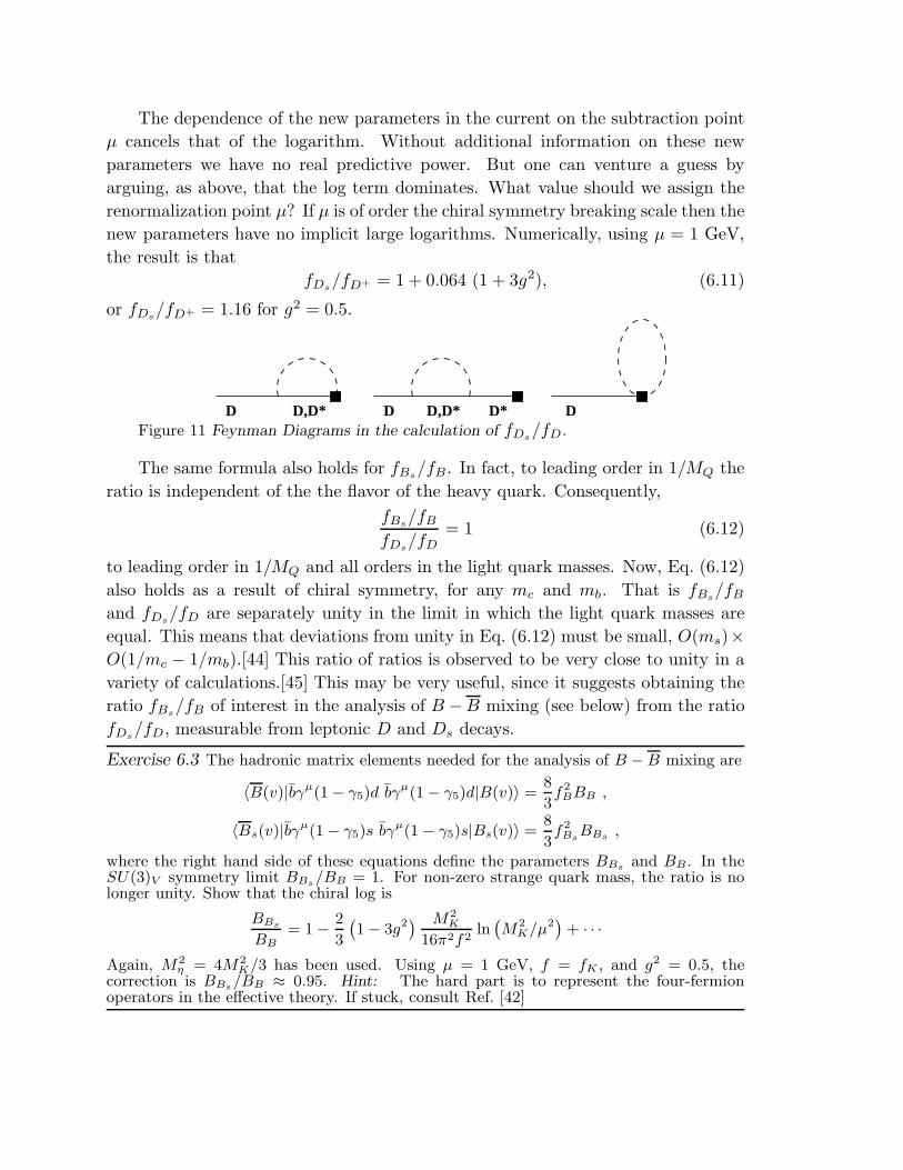
The dependence of the new parameters in the current on the subtraction point
µ cancels that of the logarithm. Without additional information on these new
parameters we have no real predictive power. But one can venture a guess by
arguing, as above, that the log term dominates. What value should we assign the
renormalization point µ? If µ is of order the chiral symmetry breaking scale then the
new parameters have no implicit large logarithms. Numerically, using µ = 1 GeV,
the result is that
fDs/fD+ = 1 + 0.064 (1 + 3g2), (6.11)
or fDs/fD+ = 1.16 for g2 = 0.5.
DD,D*D D*D,D*DFigure 11 Feynman Diagrams in the calculation of fDs
/fD.
The same formula also holds for fBs/fB. In fact, to leading order in 1/MQ the
ratio is independent of the the flavor of the heavy quark. Consequently,
fBs/fB
fDs/fD
= 1 (6.12)
to leading order in 1/MQ and all orders in the light quark masses. Now, Eq. (6.12)
also holds as a result of chiral symmetry, for any mc and mb. That is fBs/fB
and fDs/fD are separately unity in the limit in which the light quark masses are
equal. This means that deviations from unity in Eq. (6.12) must be small, O(ms)×O(1/mc − 1/mb).[44] This ratio of ratios is observed to be very close to unity in a
variety of calculations.[45] This may be very useful, since it suggests obtaining the
ratio fBs/fB of interest in the analysis of B −B mixing (see below) from the ratio
fDs/fD, measurable from leptonic D and Ds decays.
Exercise 6.3 The hadronic matrix elements needed for the analysis of B −B mixing are
〈B(v)|bγµ(1 − γ5)d bγµ(1 − γ5)d|B(v)〉 =
8
3f2
BBB ,
〈Bs(v)|bγµ(1 − γ5)s bγµ(1 − γ5)s|Bs(v)〉 =
8
3f2
BsBBs ,
where the right hand side of these equations define the parameters BBs and BB. In theSU(3)V symmetry limit BBs/BB = 1. For non-zero strange quark mass, the ratio is nolonger unity. Show that the chiral log is
BBs
BB
= 1 − 2
3
(1 − 3g2
) M2K
16π2f2ln(M2
K/µ2)
+ · · ·
Again, M2η = 4M2
K/3 has been used. Using µ = 1 GeV, f = fK , and g2 = 0.5, thecorrection is BBs/BB ≈ 0.95. Hint: The hard part is to represent the four-fermionoperators in the effective theory. If stuck, consult Ref. [42]
Violations to chiral symmetry in B → D semileptonic decays have also been
studied. One obtains that a different Isgur-Wise function must be used for each
flavor of light spectator quark[43]
ξs(v·v′)ξu,d(v·v′)
= 1 +5
3g2Ω(v·v′) M2
K
16π2f2ln(M2
K/µ2)
+ λ′(µ, v·v′)M2K + · · · (6.13)
where λ′(µ, v·v′) is the analytic counter-term, and
Ω(x) = −1 +2 + x
2√x2 − 1
ln
(x+ 1 +
√x2 − 1
x+ 1−√x2 − 1
)+
x
4√x2 − 1
ln
(x−√x2 − 1
x+√x2 − 1
)
or, expanding about x = 1,
Ω(x) = −1
3(x− 1) +
2
15(x− 1)2 − 2
35(x− 1)3 + · · ·
Using g2 = 0.5 and µ = 1 GeV, and neglecting the counterterm one obtains
ξs(v·v′)ξu,d(v·v′)
= 1− 0.21 Ω(v·v′) + · · ·
or a 5% correction at v·v′ = 2.
Exercise 6.4 Display the Feynman graphs that contribute to the ratio in Eq. (6.13).
6.4. Violations To Heavy Quark Symmetry
In a similar spirit one can consider the corrections in chiral perturbation theory
to predictions that follow from heavy quark spin and flavor symmetries. These are
effects that enter at order 1/MQ, so the first step towards this end is to supplement
the phenomenological lagrangian with such terms. In particular, there are SU(3)V
preserving terms of order 1/MQ that violate spin symmetry in the lagrangian, such
as[42,46]
∆Lint =λ2
MQTrH
(Q)aσµνH(Q)
a σµν +g2MQ
Tr[Ha(v)/Abaγ5Hb(v)
]. (6.14)
In addition there are contributions to the lagrangian in order 1/MQ that violate
flavor but not spin symmetries. These can be characterized as introducing MQ
dependence in the couplings g, λ1 and λ′1 of Eqs. (6.3) and (6.6). At the same order
as these corrections, there is a term that violates both spin and SU(3)V symmetries
∆Lint =λ3
MQTr[H
(Q)aσµνH
(Q)b σµν
] [ξmqξ + ξ†mqξ
†]ba (6.15)
Exercise 6.5 Make a complete analysis of terms that violate SU(3)V and heavy-quarksymmetries simultaneously, to leading order in both mq and 1/MQ. Note that our list isshorter since we are going to concentrate shortly on the spectrum only.
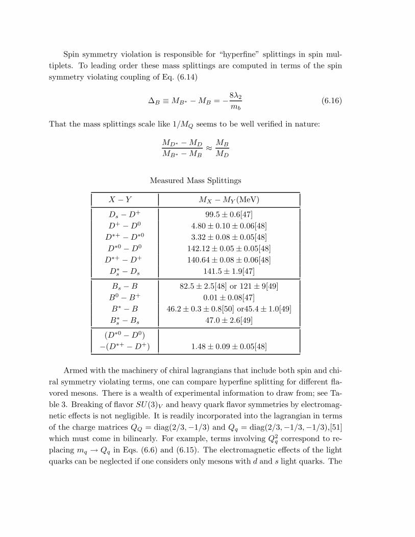
Spin symmetry violation is responsible for “hyperfine” splittings in spin mul-
tiplets. To leading order these mass splittings are computed in terms of the spin
symmetry violating coupling of Eq. (6.14)
∆B ≡MB∗ −MB = −8λ2
mb(6.16)
That the mass splittings scale like 1/MQ seems to be well verified in nature:
MD∗ −MD
MB∗ −MB≈ MB
MD
Measured Mass Splittings
X − Y MX −MY (MeV)
Ds −D+ 99.5± 0.6[47]
D+ −D0 4.80± 0.10± 0.06[48]
D∗+ −D∗0 3.32± 0.08± 0.05[48]
D∗0 −D0 142.12± 0.05± 0.05[48]
D∗+ −D+ 140.64± 0.08± 0.06[48]
D∗s −Ds 141.5± 1.9[47]
Bs −B 82.5± 2.5[48] or 121± 9[49]
B0 −B+ 0.01± 0.08[47]
B∗ −B 46.2± 0.3± 0.8[50] or45.4± 1.0[49]
B∗s −Bs 47.0± 2.6[49]
(D∗0 −D0)
−(D∗+ −D+) 1.48± 0.09± 0.05[48]
Armed with the machinery of chiral lagrangians that include both spin and chi-
ral symmetry violating terms, one can compare hyperfine splitting for different fla-
vored mesons. There is a wealth of experimental information to draw from; see Ta-
ble 3. Breaking of flavor SU(3)V and heavy quark flavor symmetries by electromag-
netic effects is not negligible. It is readily incorporated into the lagrangian in terms
of the charge matrices QQ = diag(2/3,−1/3) and Qq = diag(2/3,−1/3,−1/3),[51]
which must come in bilinearly. For example, terms involving Q2q correspond to re-
placing mq → Qq in Eqs. (6.6) and (6.15). The electromagnetic effects of the light
quarks can be neglected if one considers only mesons with d and s light quarks. The
electromagnetic shifts in the hyperfine splittings ∆Xqand ∆Xq
(X = D,B, q = d, s)
differ on account of different b and c charges, but they cancel in the difference of
splittings
∆Xs−∆Xd
= (MX∗
s−MXs
)− (MX∗
d−MXd
)
The only term in the phenomenological lagrangian that enters this difference is
Eq. (6.15). This immediately leads to
(MB∗
s−MBs
)− (MB∗
d−MBd
) =mc
mb
(αs(mc)
αs(mb)
)925 [
(MD∗
s−MDs
)− (MD∗
d−MDd
)]
(6.17)
We have included here the short distance QCD effect.[27]
One expects Eq. (6.17) holds to much better accuracy than the separate rela-
tions for each hyperfine splitting in Eq. (6.16). Recall that SU(3)V breaking by
light quark masses and electromagnetic interactions have been accounted for in
leading order. Moreover, the result is trivially generalized by replacing the quark
mass matrix in Eqs. (6.6) and (6.15), by an arbitrary function of the light quark
mass matrix. It is seen from Table 3 that this relation works well. The left side is
1.2± 2.7 MeV while the right side is 3.0± 6.3 MeV.
Since both sides of Eq. (6.17) are consistent with zero and both are propor-
tional to the interaction term in Eq. (6.15), it must be that the coupling λ3 is very
small.[51] From the difference of hyperfine splittings in the charm sector
−8λ3
mc(ms −md) = 0.9± 1.9 MeV
while
MDs−MDd
= 4λ1(ms −md)−12λ3
mc(ms −md) = 99.5± 0.6 MeV
leading to |λ3/λ1| less than ∼ 20 MeV. This is smaller than expected by about an
order of magnitude. With such a small coefficient it is clear that the next-to-leading
terms and the loop corrections may play an important role. In particular they may
invalidate the simple 1/MQ scaling of Eq. (6.17).[52] There is no obvious breakdown
of chiral perturbation theory, even though the leading coupling (λ3) is anomalously
small.[53]
At one loop, the expressions for the mass shifts involve large O(ms lnms) and
O(m3/2s ) (non-analytic) terms.[43,53] The coupling λ3 is not anomalously small at
one loop. Instead, the smallness of the difference of hyperfine splittings in Eq. (6.17)
is the result of a precise cancellation between one loop and tree level graphs. Ex-
plicitly,[53]
(MXs
−MX∗
s
)−(MXd
−MX∗
d
)=
5
3g2
(8λ2
MQ
)M2
K
16π2f2ln(M2
K/µ2)− 8λ3
MQms
With g2 = 0.5 and µ = 1 GeV, the chiral log is 30 MeV, so the λ3 counterterm
must cancel this to a precision of better than 10%.
The 1/MQ corrections to the masses MX and MX∗ drop out of the combination
MX + 3MX∗ . The combination (MXs+ 3MX∗
s) − (MXd
+ 3MX∗
d) is a measure of
SU(3)V breaking by a non-vanishing ms (or ms − md if the d quark mass is not
neglected). It can be computed in the phenomenological lagrangian. To one loop[53]
1
4
(MXs
+ 3MX∗
s
)− 1
4
(MXd
+ 3MX∗
d
)= 4λ1ms − g2
(1 +
8
3√
3
1
2
)M3
K
16πf2
−4λ1ms
(25
18+
9
2g2
)M2
K
16π2f2ln(M2
K/µ2)
(6.18)
The pseudoscalar splittings (MDs−MDd
) and (MBs−MBd
) have been measured;
see Table 3. Also, 14(MXs
+3MX∗
s)− 1
4(MXd
+3MX∗
d) = 3
4[(MX∗
s−MXs
)− (MX∗
d−
MXd)] + (MXs
−MXd), and the term in square brackets is less than a few MeV, as
we saw above. The combination (MXs+ 3MX∗
s)− (MXd
+ 3MX∗
d) in Eq. (6.18) is
first order in ms but has no corrections at order 1/MQ. Thus, one expects a similar
numerical result for B and D systems. Experimentally, (MBs−MBd
)/(MDs−MDd
)
is consistent with unity; see Table 3. The formula in Eq. (6.18) has a significant
contribution from the M3K term which is independent of the splitting parameter
λ1. The M3K term gives a negative contribution to the splitting of ∼ −250 MeV
for g2 = 0.5. The chiral logarithmic correction effectively corrects the tree level
value of the parameter λ1; for µ = 1 GeV and g2 = 0.5, the term 4λ1ms gets a
correction ≈ 0.9 times its tree level value. Thus, the one-loop value of 4λ1ms can
be significantly greater than the value determined at tree-level of approximately
100 MeV.
Chiral perturbation theory can be used to estimate the leading corrections to
the form factors for semileptonic B → D or D∗ decays which are generated at low
momentum, below the chiral symmetry breaking scale. Of particular interest are
corrections to the predicted normalization of form factors at zero recoil, v·v′ = 1.
According to Luke’s theorem (see Section 4.4), long distance corrections enter first
at order 1/M2Q. Deviations from the predicted normalization of form factors that
arise from terms of order 1/M2Q in either the lagrangian or the current are dictated
by non-perturbative physics. But there are computable corrections that arise from
the terms of order 1/MQ in the lagrangian. These must enter at one-loop, since
Luke’s theorem prevents them at tree level, and result from the spin and flavor
symmetry breaking in the hyperfine splittings ∆D and ∆B . Retaining only the
dependence on the larger ∆D, the correction to the matrix elements at zero recoil
are[54]
〈D(v)|J cbµ |B(v)〉 = 2vµ
(1− 3g2
2
(∆D
4πf
)2 [F (∆D/Mπ) + ln(µ2/M2
π)]+ C(µ)/m2
c
)
(6.19a)
〈D∗(v, ǫ)|J cbµ |B(v)〉 = 2ǫ∗µ
(1− g2
2
(∆D
4πf
)2 [F (−∆D/Mπ) + ln(µ2/M2
π)]+ C′(µ)/m2
c
)
(6.19b)
where C and C′ stand for tree level counter-terms and
F (x) ≡∫ ∞
0
dzz4
(z2 + 1)3/2
(1
[(z2 + 1)1/2 + x]2− 1
z2 + 1
)(6.20)
As before, no large logarithms will appear in the functions C and C′ if one takes
µ ≈ 4πf ∼ 1 GeV. With this choice, formally, their contributions are dwarfed by the
term that is enhanced by a logarithm of the pion mass. Numerically, with g2 = 0.5
the logarithmically enhanced term is −2.1% and −0.7% for D and D∗, respectively.
The function F accounts for effects of order (1/mc)2+n, n = 1, 2, . . . It is
enhanced by powers of 1/Mπ over terms that have been neglected. Consequently it is
expected to be a good estimate of higher order 1/mc corrections. With ∆D/Mπ ≈ 1,
one needs F (1) = 14/3− 2π and F (−1) = 14/3+ 2π for a numerical estimate; with
µ and g2 as above, this term is 0.9% and −2.0% for D and D∗, respectively.
To put it differently, if the function F is expanded in powers of 1/mc, then
since the resulting terms have inverse powers of 1/Mπ they cannot be confused
with local counterterms. These terms play the same role as the non-analytic logs
of the previous sections.
6.5. Trouble On The Horizon?
Frequently the non-analytic corrections to relations that follow from the sym-
metries are uncomfortably large. A case of much interest is the relation between
the form factors f± and h for B → K transitions, relevant to the short distance
process b→ se+e−,
〈K(pK) | sγµb |B(pB)〉 = f+ (pB + pK)µ + f− (pB − pK)µ ,
〈K(pK) | sσµνb |B(pB)〉 = ih [(pB + pK)µ(pB − pK)ν − (pB + pK)ν(pB − pK)µ] ,
and the form factors for B → πeν,
〈π(pπ) | uγµb |B(pB)〉 = f+ (pB + pπ)µ + f− (pB − pπ)µ .
In the combined large mass and chiral limits only one of these form factors is
independent:
mbh = f+ = −f− = f+ = −f− (6.21)
In this limit, the ratio of rates for B → Ke+e− and B → πeν is simply given,
in the standard model of electroweak interactions, by |Vts/Vub|2, times a pertur-
batively computable function of the top quark mass. If the relation (6.21) held
to good accuracy one could thus measure a ratio of fundamental standard model
parameters.6
The non-analytic, one-loop corrections to the relations in Eq. (6.21) have been
computed.[56] The results are too lengthy to display here. Numerically, the violation
to SU(3)V symmetry is found to be at the 40% level.7
The phenomenological lagrangian that we have been considering extensively
neglects the effects of states with heavy-light quantum numbers other than the
pseudoscalar – vector-meson multiplet. The splitting between multiplets is of the
order of 400 MeV and is hardly negligible when one considers SU(3)V relations
involving both π and K mesons. For example, consider the effect of the scalar –
6 Another application of this relation has been discussed by I. Dunietz[55]. Assuming
factorization in B → ψX, ratios of CKM elements can be extracted from these two body
hadronic decays.7 The large violation of SU(3)V symmetry affects as well the results of Dunietz (see
previous footnote).
pseudovector-meson multiplet. One can incorporate its effects into the phenomeno-
logical lagrangian. To this end, assemble its components into a “superfield”, akin
to that in Eq. (6.1) for the pseudoscalar – vector multiplet:[57]
Sa(v) =1 + v/
2
[B′µ
1aγµγ5 −B∗
0a
]. (6.22)
The phenomenological lagrangian has to be supplemented with a kinetic energy and
mass for S,
Tr[Sa(v)(iv ·Dba −∆δba)Sb(v)
],
where ∆ is the mass splitting for the excited S from the ground state H, and with
coupling terms
g′ Tr[Sa(v)Sb(v)A/baγ
5]+ (hTr
[Ha(v)Sb(v)A/baγ
5]+ h.c.) .
In terms of these one can now compute additional corrections to quantities such
as fDs/fD in Eq. (6.10). Numerically the corrections are not small,[58] fDs
/fD =
1 + 0.13h2 for MD∗
0= 2300 MeV (or fDs
/fD = 1 + 0.08h2 for MD∗
0= 2400 MeV),
assuming the strange mesons to be 100 MeV heavier. Similarly, corrections to the
Isgur-Wise function can be computed, and are not negligible.[58]
7. Acknowledgments
This work is supported in part by a Sloan Foundation Fellowship and by the
Department of Energy grant DOE-FG03-90ER40546.
References
[1] M.S. Alam, et al., the CLEO Collaboration, First Measurement Of The Rate
For The Inclusive Radiative Penguin Decay b→ sγ, CLNS-94-1314, Dec 1994.
[2] E. Witten, Nucl. Phys. B122 (1977) 109
[3] G. Altarelli and L. Maiani, Phys. Lett. 52B (1974) 351
[4] M. K. Gaillard and B. W. Lee, Phys. Rev. Lett. 33 (1974) 108
[5] E. Eichten and B. Hill, Phys. Lett. B234 (1990) 511
[6] B. Grinstein, Nucl. Phys. B339 (1990) 253
[7] H. Georgi, Phys. Lett. B240 (1990) 447
[8] M. Dugan, M. Golden and B. Grinstein, Phys. Lett. B282 (142) 1992
[9] N. Isgur and M.B. Wise, Phys. Lett. B232 (1989) 113; Phys. Lett. B237 (1990)
527
[10] S. Nussinov and W. Wetzel, Phys. Rev. D36 (1987) 130
[11] M.B. Voloshin and M.A. Shifman, Sov. J. Nucl. Phys. 47 (1988) 511
[12] E. Eichten and F. L. Feinberg, Phys. Rev. Lett. 43 (1979) 1205;;
idem, Phys. Rev. D23 (1981) 2724
[13] G. Lepage and B.A. Thacker, Nucl. Phys. B(Proc. Suppl.)4 (1988) 199
[14] C. Carone, Phys. Lett. 253B (1991) 408
[15] N. Isgur and M. B. Wise, Phys. Rev. Lett. 66 (1991) 1132
[16] A. F. Falk, et al, Nucl. Phys. B343 (1990) 1
[17] A. F. Falk, Nucl. Phys. B378 (1992) 79
[18] J. D. Bjorken and S. D. Drell, Relativistic Quantum Fields, McGraw-Hill Book
Co., 1965
[19] Boucaud, P., et al, Phys. Lett. B220 (1989) 219;
Allton, C. R., et al, Nucl. Phys. B349 (1991) 598
[20] N. Isgur and M.B. Wise, Nucl. Phys. B348 (1991) 276;
H. Georgi, Nucl. Phys. B348 (1991) 293;
T. Mannel, W. Roberts and Z. Ryzak, Nucl. Phys. B355 (1991) 38; Phys. Lett.
B255 (1991) 593
[21] B. Grinstein, Ann. Rev. Nucl. Part. Sc.,
42 (1992) 101
[22] T. Appelquist and J. Carrazone, Phys. Rev. D11 (1975) 2856
[23] M.B. Voloshin and M.A. Shifman, Sov. J. Nucl. Phys. 45 (1987) 292
[24] H.D. Politzer and M.B. Wise, Phys. Lett. B206 (1988) 681
[25] A. F. Falk and B. Grinstein, Phys. Lett. B249 (1990) 314
[26] G.P. Korchemskii and A.V. Radyushkin , Phys. Lett. B279 (1992) 359
[27] A. Falk, B. Grinstein and M. Luke, Nucl. Phys. B357 (1991) 185
[28] A. Falk and B. Grinstein, Phys. Lett. B247 (1990) 406
[29] E. Eichten and B. Hill, Phys. Lett. B243 (1990) 427
[30] M. Golden and B. Hill, Phys. Lett. B254 (1991) 225
[31] H. Georgi, B. Grinstein and M. B. Wise, Phys. Lett. 252B (1990) 456
[32] M.E. Luke, Phys. Lett. B252 (1990) 447
[33] P. Cho and B. Grinstein, Phys. Lett. B285 (1992) 153
[34] A good introduction can be found in H. Georgi, Weak Interactions and Mod-
ern Particle Physics(The Benjamin/Cummings Publishing Company, Califor-
nia,1984)
[35] G. Burdman, J. F. Donoghue, Phys. Lett. B280 (1992) 287;
M. B. Wise, Phys. Rev. D45 (1992) 2188
[36] T.-M. Yan, H.-Y. Cheng, C.-Y. Cheung, G.-L. Lin, Y. C. Lin and H.-L. Yu,
Phys. Rev. D46 (1992) 1148
[37] The ACCMOR Collaboration (S. Barlag et al), Phys. Lett. B278 (1992) 480
[38] The CLEO Collaboration (F. Butler et al), Phys. Rev. Lett. 69 (1992) 2041
[39] J. Amundson, C. Boyd, E. Jenkins, M. Luke, A. Manohar, J. Rosner, M. Savage
and M. Wise, Phys. Lett. B296 (1992) 415;
P. Cho and H. Georgi, Phys. Lett. B296 (1992) 408
[40] H.-Y. Cheng, C.-Y. Cheung, G.-L. Lin, Y. C. Lin, T.-M. Yan and H.-L. Yu,
Phys. Rev. D46 (1992) 5060
[41] The CLEO Collaboration (D. Acosta, et al,), First Measurement Of Γ(D+s →
µ+ν)/Γ(D+s → φπ+), CLNS-93-1238, Aug 1993.
[42] B. Grinstein, E. Jenkins, A. Manohar, M. Savage and M. Wise, Nucl. Phys.
B380 (1992) 369
[43] J. Goity, Phys. Rev. D46 (1992) 3929
[44] B. Grinstein, Phys. Rev. Lett. 71 (1993) 3067
[45] See, for example, C. Bernard, J. Labrenz and A. Soni, Phys. Rev. D49 (1994)
2536;
C. Dominguez, Phys. Lett. B318 (1993) 629
[46] C. G. Boyd and B. Grinstein, Chiral and Heavy Quark Symmetry Violation in B
Decays, UCSD/PTH 93-46, SMU-HEP/94-03, SSCL–Preprint–532, Feb. 1994
(hep-ph/9402340)
[47] Particle Data Group, Phys. Rev. D45 (1992)
[48] The Cleo Collaboration (D. Bortoletto et al) Phys. Rev. Lett. 69 (1992) 2046

[49] The CUSB-II Collaboration (J. Lee-Franzini et al), Phys. Rev. Lett. 65 (1990)
2947
[50] The Cleo II Collaboration (D.S. Akerib et al), Phys. Rev. Lett. 67 (1991) 1692
[51] J. Rosner and M. Wise, Phys. Rev. D47 (1992) 343
[52] L. Randall and E. Sather, Phys. Lett. B303 (1993) 345
[53] E. Jenkins, Nucl. Phys. B412 (1994) 181
[54] L. Randall and M. Wise, Phys. Lett. B303 (1993) 135
[55] I. Dunietz, Extracting CKM parameters from B decays, in Proceedings of the
Workshop on B Physics at Hadron Accelerators, Snowmass Colo., 1993
[56] A. Falk and B. Grinstein, Nucl. Phys. B416 (1994) 771
[57] A. Falk, Nucl. Phys. B378 (1992) 79;
A. Falk and M. Luke, Phys. Lett. B292 (1992) 119
[58] A. Falk, Phys. Lett. B305 (1993) 268


