Seediscussions,stats,andauthorprofilesforthispublicationat:https://www.researchgate.net/publication/5030124

AnInternationalPerspectiveonOilPriceShocksandU.S.EconomicActivity

ARTICLE·FEBRUARY2008

Source:RePEc

CITATIONS

2

READS

13

3AUTHORS,INCLUDING:

NathanBalke

SouthernMethodistUniversity

59PUBLICATIONS2,030CITATIONS

SEEPROFILE

MineK.Yücel

88PUBLICATIONS769CITATIONS

SEEPROFILE

Availablefrom:NathanBalke

Retrievedon:03February2016

Federal Reserve Bank of Dallas Globalization and Monetary Policy Institute

Working Paper No. 20 http://www.dallasfed.org/institute/wpapers/2008/0020.pdf

An International Perspective on Oil Price Shocks and U.S. Economic Activity*

Nathan S. Balke

SMU and Federal Reserve Bank of Dallas

Stephen P. A. Brown Federal Reserve Bank of Dallas

Mine K. Yücel

Federal Reserve Bank of Dallas

September 2008 Abstract The effect of oil price shocks on U.S. economic activity seems to have changed since the mid-1990s. A variety of explanations have been offered for the seeming change—including better luck, the reduced energy intensity of the U.S. economy, a more flexible economy, more experience with oil price shocks and better monetary policy. These explanations point to a weakening of the relationship between oil prices shocks and economic activity rather than the fundamentally different response that may be evident since the mid-1990s. Using a dynamic stochastic general equilibrium model of world economic activity, we employ Bayesian methods to assess how economic activity responds to oil price shocks arising from supply shocks and demand shocks originating in the United States or elsewhere in the world. We find that both oil supply and oil demand shocks have contributed significantly to oil price fluctuations and that U.S. output fluctuations are derived largely from domestic shocks. JEL codes: F41, Q43

* Nathan S. Balke, Department of Economics, Southern Methodist University, Dallas, TX 75275(nbalke@mail.smu.edu); Stephen P. A. Brown, Research Department, Federal Reserve Bank of Dallas 2200 North Pearl Street, Dallas, TX 75201 (spa.brown@yahoo.com); Mine K. Yücel, Research Department, Federal Reserve Bank of Dallas, 2200 North Pearl Street, Dallas TX 75201 (mine.k.yucel@dal.frb.org). The authors thank Mario Crucini, Fred Joutz, Luca Guerrieri, William Helkie,Lutz Kilian, Prakash Loungani, Erwan Quintin, Tara Sinclair, Mark Wynne and Carlos Zarazaga for helpful comments and discussions and Stefan Avdjiev and Zheng Zeng for capable research assistance. The authors retain all responsibility for omissions and errors. The views expressed are those of the authors and should not be attributed to the Federal Reserve Bank of Dallas, the Federal Reserve System or Southern Methodist University.

1

An International Perspective on Oil Price Shocks and U.S. Economic Activity

Abstract: The effect of oil price shocks on U.S. economic activity seems to have changed since the mid-1990s. A variety of explanations have been offered for the seeming change—including better luck, the reduced energy intensity of the U.S. economy, a more flexible economy, more experience with oil price shocks and better monetary policy. These explanations point to a weakening of the relationship between oil prices shocks and economic activity rather than the fundamentally different response that may be evident since the mid-1990s. Using a dynamic stochastic general equilibrium model of world economic activity, we employ Bayesian methods to assess how economic activity responds to oil price shocks arising from supply shocks and demand shocks originating in the United States or elsewhere in the world. We find that both oil supply and oil demand shocks have contributed significantly to oil price fluctuations and that U.S. output fluctuations are derived largely from domestic shocks. 1. Introduction

Since early 2003, the price of crude oil has nearly quadrupled, increasing from around

$30 per barrel (for West Texas Intermediate crude oil) to about $115 in late summer 2008. In

addition to little excess OPEC production capacity, an uncertainty premium brought about by

geopolitical tensions, and a weak dollar; part of the strength in oil prices is attributed to the

strength of Chinese, Indian, U.S. and European oil demand and to expectations that world oil

demand will grow faster than supply over coming decades.

Since World War II, oil prices have gone hand-in-hand with U.S. recessions. In fact, nine

of the ten post-WWII recessions have been preceded by episodes of sharply rising oil prices

(Figure 1). The 1960 recession is the one exception.

Economic research has long documented a relationship between oil price shocks and

slowing U.S. economic activity, with the consequences being slower GDP growth and possible

recession, higher unemployment rates, and a higher price level. Some of the earlier studies

include Pierce and Enzler (1974), Rasche and Tatom (1977), Mork and Hall (1980), Gisser and

Goodwin (1986) and the Energy Modeling Forum 7 study documented in Hickman et al. (1987).

2

Darby (1982), Burbidge and Harrison (1984), and Bruno and Sachs (1982, 1985)

documented similar oil-price-economy relationships for countries other than the United States.

Hamilton (1983) extended the analysis period to show that all but one of the U.S. post-WWII

recessions were preceded by sharply rising oil prices. The apparent lack of a favorable response

of economic activity to falling oil prices led to later studies—such as Ferderer (1996), Hamilton

(1996, 2003), Davis and Haltiwanger (2001) and Balke, Brown and Yücel (2002)—that allowed

for an asymmetric relationship between oil price shocks and economic activity.

Several studies contend that the apparent relationship between oil price shocks and

aggregate economic activity comes through monetary policy. Bohi (1989, 1991) and Bernanke,

Gertler and Watson (1997) argue that a contractionary monetary policy response to oil price

shocks accounted for much of the decline in aggregate economic activity following an oil price

increase. In a somewhat different vein, Barsky and Kilian (2001, 2004) contend that swings

between expansionary and contractionary monetary policy created cycles in which rising oil

prices preceded but did not cause the economic downturns of the 1970s and 80s.

A number of other studies accord a much smaller role to monetary policy. Ferderer

(1996) provides evidence that counter-inflationary monetary policy was only partially

responsible for the real effects of oil price shocks over the period from 1970 to 1990. Davis and

Haltiwanger (2001) showed that the effect of oil price shocks on employment growth were twice

that of monetary policy shocks. Brown and Yücel (1999) argue that monetary policy wasn’t

necessarily contractionary. Hamilton and Herrera (2004) show that the reduction in interest rates

necessary to offset the aggregate effects of rising oil prices are outside historical experience, and

Herrera and Pesavento (forthcoming) find that monetary policy a had much smaller effect than

that estimated by Bernanke, Gertler and Watson.

3

Although the relationship between oil prices and economic activity seemed fairly robust

and reasonably well understood by the mid-1990s, the relationship seemed to have weakened in

the late 1990s and the 2000s—as shown by the relationship between oil prices and the cyclical

component of GDP (Figure 2). The increase in oil prices in the early 1970s, the tripling of oil

prices in 1979 and the sharp oil-price gains during the first Iraq war preceded declines in the

cyclical component of real GDP. Since the mid-1990s, however, episodes of sharp oil price

increases have not led declines in the cyclical component of real GDP—with the most noticeable

period being since 2003 when oil prices more than quadrupled.

The apparent weakening or reversal of the past economic effects of oil price shocks has

stimulated a new literature about why the U.S. economy might respond differently to rising oil

prices in the 2000s than it did in the 1970s and early 80s.1 Contributions include Huntington

(2003), CBO (2006), Blanchard and Gali (2007), Bodenstein, Erceg and Guerrieri (2007), and

Segal (2007). The explanations include more stable aggregate demand (possibly the result of

better luck or increased global financial integration), the reduced energy intensity of the U.S.

economy, greater flexibility of the U.S. economy (including labor and financial markets),

increased experience with energy price shocks, and better monetary policy.

Most of the explanations that have been offered for a changed response to oil price

shocks treat oil price shocks as exogenous and point to quantitatively smaller effects rather than

qualitatively different effects. But exogenous oil supply shocks need not be the only forces that

push oil prices higher. Kilian (2007) identifies oil price shocks as arising from crude oil supply

shocks, shocks to global oil demand and precautionary demand associated with uncertainty about

1 A more general literature examines the increased stability of the U.S. economy since the mid-1980s, with explanations that include structural changes in the U.S. economy, better luck and improved monetary policy. See Kim and Nelson (1999a), McConnell and Perez-Quiros (2000), Blanchard and Simon (2001), Kahn, McConnell and Perez-Quiros (2002), Stock and Watson (2003), Bernanke (2004) and Boivin and Giannoni (2006).

4

oil supply shortfalls. In a similar vein, Elekdag and Laxton (2007) argue that the current oil

price increases are demand driven, while earlier increases in oil prices were supply driven.

Productivity gains can boost global economic growth and push oil prices upward at the same

time.

To analyze the effects of different types of economic shocks on aggregate economic

activity and oil prices (while treating oil prices as endogenous), we develop a dynamic stochastic

general equilibrium model of world economic activity. The model generally follows that of

Backus, Kehoe and Kydland (1992) and Backus and Crucini (2000) and represents the world

economy as two manufacturing countries and an oil-producing country. We depart from Backus

and Crucini in two important ways. First, we represent all oil production and the evolution of oil

reserves as endogenous. In our model, oil producers face dynamic tradeoffs when deciding how

much oil to produce: higher production today reduces the oil reserves available in the future. Oil

producers can invest to expand oil reserves, which increases future oil production capacity.

Second, rather than calibrate the parameters of the model and use it for a simulation exercise, we

use Bayesian methods to estimate the parameters of technology and preferences as well as the

parameters for the stochastic process generating the exogenous shocks. In the process of

estimating the parameters, we also estimate realizations for the unobserved shock processes.

The model allows us to examine empirically the effects of various types of shocks on oil

markets and aggregate economic activity. These shocks include: oil supply shocks, oil reserve

shocks, total factor productivity shocks, labor supply shocks, shocks to the economic efficiency

of oil use, and shocks in investment demand originating in the manufacturing countries. The

estimated model implies that shocks to oil production and reserves affect oil prices and output in

5

a way that is reminiscent of oil supply shocks. Shocks in manufacturing countries look like a

mixture of oil supply and demand shocks in the short run and oil demand shocks in the long run.

Historical decompositions suggest that much of the recent gains in oil prices can be

attributed to oil “demand” shocks, but the episodes of dramatic oil price increases in the 1970s

and early 1980s were attributable mainly to oil supply shocks. For the United States, the

historical decompositions suggest these oil supply shocks had only moderate effects on economic

growth. The poor economic performance in the 1970s and early 1980s appears to have resulted

mainly from the confluence of negative shocks to total factor productivity and labor supply.

For recent years, the historical decompositions suggest that oil prices and U.S. real GDP

have moved in the same direction for two reasons. Increases in total factor productivity have

boosted U.S. GDP overwhelming the negative effects of oil supply shocks. Furthermore,

improvements in the economic efficiency of oil use have simultaneously boosted U.S. GDP and

the demand for oil.

2. The Model

Following Backus and Crucini (2000), we represent the world as three countries. Two of

the countries each produce a final manufactured good. The third country produces oil, which is

an intermediate good used in the production of the manufactured goods. Departing from Backus

and Crucini, we treat oil production and the evolution of oil reserves in the oil-producing country

as completely endogenous.2 Treating oil-production and pricing as endogenous in our

framework allows us to more thoroughly examine the economic effects of total factor

productivity shocks in the two manufacturing countries, as well as to consider the economic

effects of oil supply shocks. The former is critical to distinguishing between productivity shocks

2 Backus and Crucini represent oil production as having an exogenous component (OPEC) and an endogenous supply component via a labor-only technology.

6

that could potentially increase world oil demand and prices from world oil supply shocks that

increase oil prices. In addition to making the oil sector more dynamic than is represented in the

Backus and Crucini model, we add three additional shocks that will help the model better capture

actual fluctuations in economic activity: labor wedge shocks, oil wedge shocks, and investment

shocks.

2.1 Consumers

In each of the three countries, consumers directly use the two manufactured goods and

face a labor-leisure tradeoff. Accordingly, consumers in each country j maximize lifetime

utility:

∑∞

=

=0

,, ),(t

tjtjt

j LCUE β for j = a, b, o (1)

where β is a discount factor, C is a CES aggregate of the manufactured goods A and B, each of

which is produced in countries a and b, respectively, L is leisure. Following Backus and

Crucini,σ

σθθ

−=

−−

1

11 )LC()L,C(U t,jt,j

t,jt,j for the manufacturing countries j = a,b; and

)(1

),( ,,

1,

,, tooLto

toto LvC

LCU θσ

σ

+−

=−

for the oil-producing country.

For the manufacturing countries, leisure is the amount of time available after supplying

labor to manufacturing, Lj,t = 1 - Nj,t. For the oil-producing country, leisure is the amount time

available after supplying labor to oil production and to reserve additions, Lo,t = 1 - No,t - Nx,t.

The CES consumption aggregate for each country is as follows:

)1/(11,,

1,,, ])1([ μμμ −−− Ψ−+Ψ= tjcjtjcjtj BAC for j = a, b, o (2)

7

where Ac,j,t is country j’s use of good A for consumption; Bc,j,t is the country j’s use of good B for

consumption; Ψj captures the weight households place on the consumption of goods A and B;

and μ is the elasticity of substitution between goods A and B.

When estimating the model empirically, a preference shock is also added to the model

that captures fluctuations in the wedge between the measured marginal rate of substitution

between leisure and consumption and the marginal product of labor in the two manufacturing

countries. Specifically, tjnconsumptioleisuretjNtjc

tj MRSPW

,,/,,,,

, ω= where tN ,ω is the labor wedge and

is the consumption deflator in country j. Changes in the wedge act like a labor supply

shock. This shock could reflect not only changes in preferences but also changes in wage

markups or changes in marginal tax rates. Hall (1997) and Chari, et al (2007) have argued that

fluctuations in the wedge between marginal rate of substitution and marginal product of labor

play an important role in labor market fluctuations.

tjCP ,,

2.2 Manufacturing, Production and Investment

In each of the manufacturing countries, output is a function of capital, labor, oil use and

the technology available in each time period:

υα

υυα −−

−− Ψ−+Ψ= 11

11 1 )O)(K(NZY t,jkt,jkt,jt,jt,j for j = a, b (3)

where Yj,t is country j output at time t, Kj,t is capital, Nj,t is labor, Oj,t is oil use, and Zj,t is total

factor productivity. One can think of this function as representing production as follows: oil and

capital are used to produce capital services which are combined with labor to produce goods.

The elasticity of substitution between capital and oil in the production of capital services is given

by ν/1 and will generally be different than that between capital services and labor (which is

unitary, given the Cobb-Douglas representation of the latter relationship).

8

As is done for the labor market, when taking the model to the data we add a stochastic

wedge between the measured marginal product of oil and the relative price of oil. The oil

wedge, tjo ,,ω , is defined such that tj

totjotjo P

PMP

,

,,,,, ω= where is the (measured) marginal

product of oil in the production of country j’s output. The wedge could reflect policies that

affect the true price to firms of using oil (for example, taxes or environmental regulations). The

wedge also could reflect a difference between our model-based measure of the marginal product

of oil and its true productivity—with a greater measured value of marginal product relative to

true marginal product yielding a higher value of

tjoMP ,,

tjo ,,ω , assuming the real oil price is unchanged.

The wedge acts as an additional source of fluctuations in oil demand in our empirical model.

Similar to that for consumption, the CES investment aggregate for each manufacturing

country is as follows:

)1/(11,,

1,,, ])1([ μμμ −−− Ψ−+Ψ= tjijtjijtj BAI for j = a, b (4)

where Ai,j,t is country j’s use of good A for investment, Bi,j,t is the country j’s use of good B for

investment. Capital accumulation in each of the manufacturing countries takes into account

depreciation and investment as follows:

tjKtjtjtjtjtj ZKKIKK ,,,,,,1, )/()1( +Φ+−=+ δ for j = a, b (6)

where δ is the depreciation rate and Ij,t is investment. )K/I( t,jt,jΦ is the rate at which

investment goods become capital and reflects adjustment costs in changing the stock of capital

with and . is a capital accumulation shock (similar to an additive

productivity shock to investment). One can think of this shock as reflecting shocks to investment

demand that are unrelated to the future marginal product of capital.

0>Φ′(.) 0<Φ ′′(.) tjKZ ,,

9

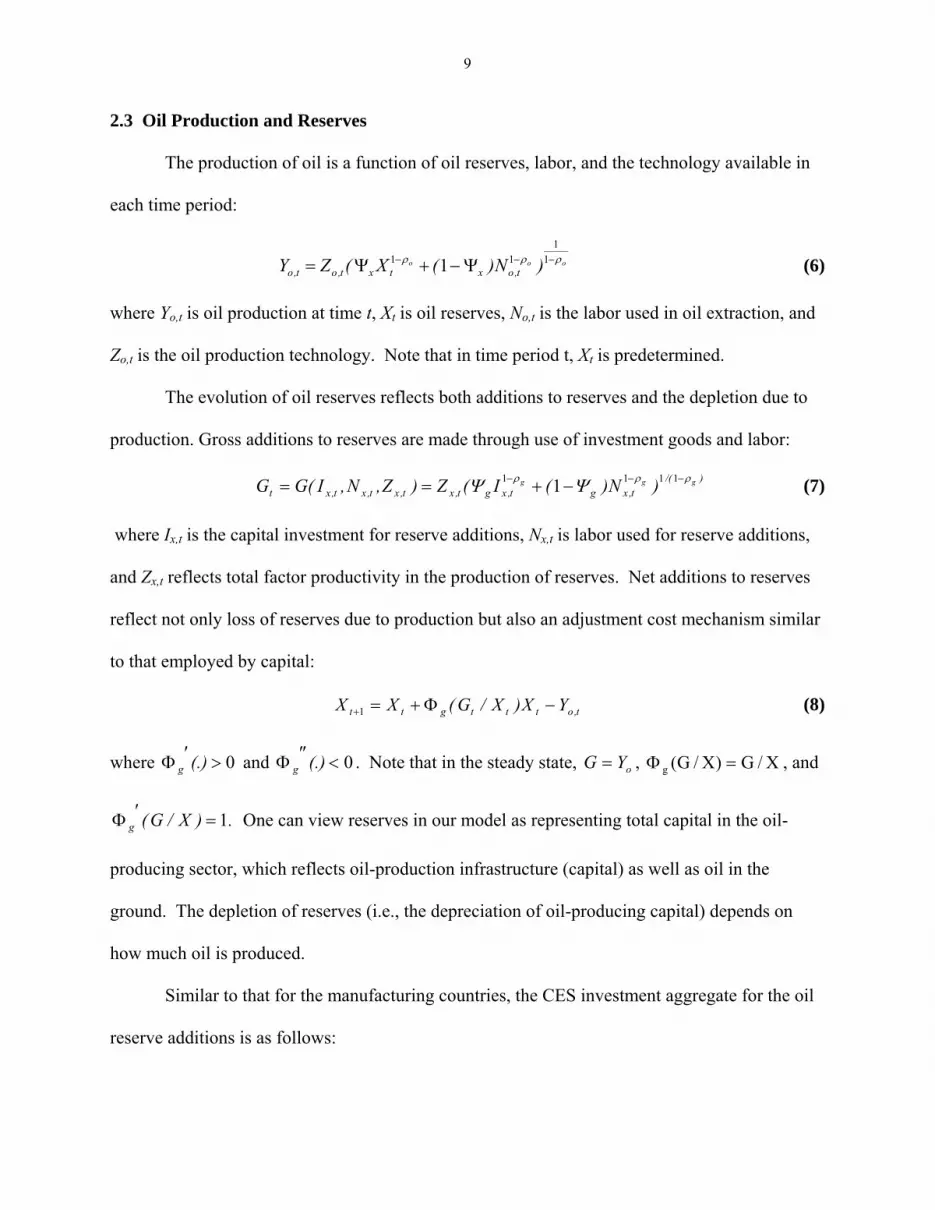
2.3 Oil Production and Reserves

The production of oil is a function of oil reserves, labor, and the technology available in

each time period:

ooo )N)(X(ZY t,oxtxt,ot,oρρρ −−− Ψ−+Ψ= 11

11 1 (6)

where Yo,t is oil production at time t, Xt is oil reserves, No,t is the labor used in oil extraction, and

Zo,t is the oil production technology. Note that in time period t, Xt is predetermined.

The evolution of oil reserves reflects both additions to reserves and the depletion due to

production. Gross additions to reserves are made through use of investment goods and labor:

)/(t,xgt,xgt,xt,xt,xt,xt

ggg )N)(I(Z)Z,N,I(GG ρρρ ΨΨ −−− −+== 1111 1 (7)

where Ix,t is the capital investment for reserve additions, Nx,t is labor used for reserve additions,

and Zx,t reflects total factor productivity in the production of reserves. Net additions to reserves

reflect not only loss of reserves due to production but also an adjustment cost mechanism similar

to that employed by capital:

t,otttgtt YX)X/G(XX −Φ+=+1 (8)

where and . Note that in the steady state, 0>′Φ (.)g 0<″Φ (.)g oYG = , X/G)X/G(g =Φ , and

One can view reserves in our model as representing total capital in the oil-

producing sector, which reflects oil-production infrastructure (capital) as well as oil in the

ground. The depletion of reserves (i.e., the depreciation of oil-producing capital) depends on

how much oil is produced.

.)X/G(g 1=′Φ

Similar to that for the manufacturing countries, the CES investment aggregate for the oil

reserve additions is as follows:

10

)1/(11,,

1,,, ])1([ μμμ −−− Ψ−+Ψ= txixtxixtx BAI (9)

where Ai,x,t is the use of the country a good in the process of making reserve additions, and Bi,x,t is

the use of the country b good in the process of making reserve additions.

2.4 International Market Clearing Constraints

In each period of time, the total quantities of each of the three goods must be completely

used:

toitbitaitoctbctacta AAAAAAY ,,,,,,,,,,,,, +++++= (10)

toitbitaitoctbctactb BBBBBBY ,,,,,,,,,,,,, +++++= (11)

tbtato OOY ,,, += (12)

In addition, market-clearing prices and wages must be established.

2.5 Exogenous Shocks

There are ten exogenous driving forces in our model. Eight shocks originate in the two

manufacturing countries. For each manufacturing country, there are shocks to total factor

productivity, the labor wedge, the oil wedge and investment. The other two shocks originate in

the oil-producing country. They are a technology shock to oil production and a technology

shock to the production of oil reserves. With the exception of total factor productivity shocks,

we assume that the (logs of the) exogenous driving forces follow independent first-order

autoregressive processes. Following Backus and Crucini (2000), we allow total factor

productivity to be correlated across manufacturing countries, both contemporaneously and with a

lagged spillover. Unlike Backus and Crucini, the stochastic processes for these variables are not

assumed to be the same across the two manufacturing countries.

11

2.6 Oil Supply Shocks

As discussed above, the model’s implementation of oil demand is similar to that found in

Backus and Crucini (2000). On the supply side, the current model differs from Backus and

Crucini by capturing both oil production and reserves.

Maximizing the representative agent’s utility in the oil-producing country, taking prices

as given, yields the following decisions rules for the production of oil and reserves. Oil

production is determined so that:

t,ot,xt,o mcpp += , (13)

where is the price of oil (in terms of the numeraire good), is the price of reserves (user

cost of oil), and is the marginal cost of producing oil in time period t. Given that the stock

of reserves is fixed in time t, where is the wage (in terms of the numeraire

good) in the oil-producing country and is the marginal product of labor in the oil-producing

country. The first order condition for the production of reserves is given by:

t,op t,xp

t,omc

ot,lt,ot,o mp/wmc = t,ow

ot,lmp

)}]1(){([1

11,1,1,1,1,1,1,

+

++++++++ Φ′−Φ++−=

t

ttgtgtx

otxtxtotttx X

GpmpppMEp , (14)

where is the stochastic discount factor and 1+tM

)}XG

(pmp)pp{(t

tt,gt,gt,x

ot,xt,xt,o

1

1111111 1

+

+++++++ Φ′−Φ++− is the payoff of having more reserves

next period. The term is the value of using those reserves to produce oil

next period while

111 +++ − t,xt,xt,o mp)pp(

)XG

(pt

tt,gt,gt,x

1

1111 1

+

++++ Φ′−Φ+ is the value of additional reserves at the end of

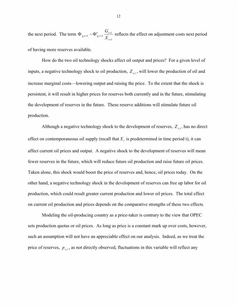
12

the next period. The term 1

111

+

+++ Φ′−Φ

t

tt,gt,g X

G reflects the effect on adjustment costs next period

of having more reserves available.

How do the two oil technology shocks affect oil output and prices? For a given level of

inputs, a negative technology shock to oil production, , will lower the production of oil and

increase marginal costs—lowering output and raising the price. To the extent that the shock is

persistent, it will result in higher prices for reserves both currently and in the future, stimulating

the development of reserves in the future. These reserve additions will stimulate future oil

production.

t,oZ

Although a negative technology shock to the development of reserves, , has no direct

effect on contemporaneous oil supply (recall that is predetermined in time period t), it can

affect current oil prices and output. A negative shock to the development of reserves will mean

fewer reserves in the future, which will reduce future oil production and raise future oil prices.

Taken alone, this shock would boost the price of reserves and, hence, oil prices today. On the

other hand, a negative technology shock in the development of reserves can free up labor for oil

production, which could result greater current production and lower oil prices. The total effect

on current oil production and prices depends on the comparative strengths of these two effects.

t,xZ

tX

Modeling the oil-producing country as a price-taker is contrary to the view that OPEC

sets production quotas or oil prices. As long as price is a constant mark up over costs, however,

such an assumption will not have an appreciable effect on our analysis. Indeed, as we treat the

price of reserves, , as not directly observed, fluctuations in this variable will reflect any txp ,

13

fluctuations in the mark-up of oil prices over marginal costs.3 Thus, changes in OPEC’s price

setting stance will in part be captured by our measures of technology shocks to oil production

and reserve development. An exogenous cut in OPEC oil production, perhaps for geopolitical

reasons, would look like a negative technology shock to oil production.4

3. Model Solution and Estimation.

To solve the model for a given set of parameters, we log-linearize the first order

conditions of the social planner’s problem around the deterministic steady state and solve the

resulting linear rational expectations model as in Blanchard and Kahn (1980). Rather than

calibrate the parameters, we use Bayesian methods to estimate the parameters of technology,

preferences, and the stochastic processes generating the exogenous shocks.

As in Backus and Crucini, we take the United States to be one of the manufacturing

countries in the model. The other manufacturing country denoted below by ROW, we take to be

the OECD countries (less Mexico and the United States) plus Brazil, China, and India. We take

the time interval of the model to be quarterly and include eight quarterly time series in the

estimation of the model. These inclue: real oil prices (deflated by the U.S. GDP deflator), world

oil production, U.S. real GDP, U.S. real consumption, U.S. real investment, U.S. hours, U.S. oil

consumption and the relative price of imports to the United States.

While the relative price of U.S. imports, U.S. oil consumption and world oil production

provide the information about economic activity in the ROW, it would be useful to include more

direct information on economic activity in ROW. Unfortunately, there are not quarterly data of

sufficient length for many countries to construct a quarterly series for the ROW. Because our

3 Petroleum Intelligence Weekly and the Oil and Gas Journal provide some data on the sales of reserves, but these prices may not be representative of overall market conditions because most reserves—particularly those of OPEC—are not traded, and the value of reserves may vary considerably with the characteristics of the reserves. 4 This abstracts from the cross-country wealth effect of an increase in the markup of oil prices.

14

estimation procedure readily handles the use of mixed frequency data (see appendix), however,

we add annual ROW output and investment (in constant dollars) as two additional observation

equations. Thus, taken together we have eight quarterly observation equations and two annual

observation equations.5 Our sample period runs from 1970 through 2006.

The linearized DSGE model links the observed time series and the underlying driving

processes that result in deviations from the steady state.6 Markov Chain Monte Carlo methods

similar to those of Lubik and Schorfheide (2004) and Smets and Wouters (2007) are employed to

estimate the posterior distribution of the parameters.7 In the process of estimating the posterior

distribution of the parameters, we also estimate a posterior distribution for the unobserved shock

processes. These estimates allow us to decompose movements in actual observables into

contributions due to various exogenous shocks.

3.1 Prior and posterior distributions of the structural parameters.

In implementing the Bayesian estimation strategy, we must specify prior distributions for

the structural parameters (parameters of technology and preferences) and the parameters of the

stochastic processes of the ten exogenous driving forces. For most of the structural parameters

for the two manufacturing countries, we set the mode of the prior distribution to be equal to the

values set in Backus and Crucini. For the oil-producing country, we use information on the ratio

of oil production to reserves,XY0 , labor share in the production of oil, and the ratio of oil price to

5 For the United States and world oil, we find substantially similar results to those reported below when the model is not required to fit annual output and investment data for rest of the world. The principal difference is that use of the rest of world data allows a better identification of the individual sources of rest-of-world shocks. 6 The logs of U.S. real GDP, consumption, investment, hours, oil consumption; relative price of imports to the United States; rest of world output and investment; and world oil production are linearly detrended. The logs of real oil price are demeaned. 7 We use the random walk Metropolis-Hastings sampler to generate draws from the posterior distribution. The transition equation in the Markov Chain depends on the Hessian of the posterior distribution evaluated at the posterior mode and shocks drawn from a t-distribution with five degrees of freedom. We use 105,000 draws in our sampler with 100,000 draws as the burn in period.

15

reserve price , 00 mcp

ppp o

x

o

−= , to help set the prior distributions of the parameters. As for how

much weight to place on the prior distribution versus the data when estimating the posterior

distributions, we divide the parameters into roughly three groups. Parameters like the discount

factor or those that reflect shares of steady state values (for example, output elasticity of labor

equals labor’s share in GDP) have relatively tight priors. Parameters that reflect elasticities of

substitution or adjustment costs for capital and reserves have more diffuse priors. Finally, a third

group of parameters, namely the parameters of the stochastic processes governing the driving

forces have relatively uninformed priors—as we have very little direct prior information

concerning these stochastic processes.

Table 1 displays the prior and estimated posterior distributions of the structural

parameters. For many parameters, using the information in the data results in a substantial shift

in the posterior distribution relative to the prior distribution; for most parameters the posterior

distribution is substantially tighter than the prior distribution. Not surprisingly given the tight

priors for these parameters, the posterior distributions for the discount factor, labor’s share in

manufacturing country GDP, the share of home and foreign goods, and the depreciation rate on

capital are close to the values assumed in Backus and Crucini.

Our posterior distribution suggests an estimate of the intertemporal elasticity of

substitution which is similar to that typically assumed in the macroeconomics literature. The

posterior distribution also suggests an elasticity of substitution between domestic and the foreign

good that is substantially lower than that assumed in Backus and Crucini. 8 On the other hand,

the elasticity of substitution between oil and capital is slightly larger than in Backus and Crucini.

8 Given that Backus and Crucini calibrate their parameters to data for the United States and other OECD countries, it is not surprising that our estimated parameters take different values. In addition, the dramatic swings in the relative

16

The posterior distributions for all three of these elasticities are substantially “tighter” than their

prior distributions. The posterior distribution for the elasticities of substitution in the oil

production and reserve production technologies are still relatively “diffuse” suggesting the data

are not too informative about these parameters. Finally, the adjustment costs for capital are

estimated to be substantially higher than those for oil reserves suggesting that it is easier to add

to reserves than it is to add to capital in the manufacturing country.

Table 2 presents the prior and posterior distributions for the stochastic processes

governing the exogenous variables in the model. Given that prior distributions were relatively

uninformative, the data have a lot to say about these variables. With the exception of ROW

investment demand shocks, the autoregressive parameters are quite high suggesting that shocks

are very persistent. The standard deviation of shocks to oil production and oil reserves are

relatively large compared to shocks in total factor productivity and investment shocks in the

manufacturing countries. The standard deviation of oil wedge shocks in the two manufacturing

countries is very large suggesting that these two variables may be an important source of shocks

to world oil demand. On the other hand, the estimated spillover in total productivity is relatively

small. Finally, the variances of ROW shocks, with the exception of the investment shock, are

estimated to be larger than U.S. shocks.

3.2 Model Evaluation

To evaluate the relative fit of the model, we compare our benchmark model to a model in

which the structural parameters are set to the values assumed by Backus and Crucini (the

parameters of the shock processes are estimated as in the benchmark model) and to a state space

import price over our sample period likely contribute to a relatively low value for the elasticity of substitution between home and foreign goods.

17

model in which the state equation is a VAR(1) with relatively uninformed priors.9 We use a

state space-VAR(1) rather than a traditional VAR(1) model for comparison because we have

only annual data for rest-of-world output and investment.

To assess our model’s overall “goodness of fit”, we construct marginal likelihoods and

Bayes factors for the three models.10 These are presented in Table 3. Our benchmark model

appears to “fit” the data better than the two alternative models. As mentioned above, with the

exception of the elasticity of substitution between domestic and foreign goods, the modes of the

posterior distribution for most of the structural parameters in the benchmark model are similar to

the values assumed in Backus and Crucini. However, because of the large swings in the relative

import price over our sample, a low value for the elasticity of substitution between domestic and

foreign goods in the benchmark model substantially improves the fit of the model. The

benchmark model fits better than the state space-VAR(1) model in part because relatively diffuse

priors are assumed for the latter model’s vastly greater number of parameters. Unfortunately, we

were unable to conceive of “naturally suggestive” non-diffuse prior distributions for the reduced

form state space model that yielded an improvement over the model with diffuse priors.11

4. Impulse Responses

To obtain a better picture of what the model implies about oil shocks and economic

activity, we examine how oil markets and real U.S. GDP respond to a variety of shocks,

including a negative oil production shock, a negative oil reserve shock, a positive total factor

productivity shock, a positive labor wedge shock, a positive oil wedge shock, and a negative U.S.

9 The benchmark and Backus and Crucini models are evaluated assuming the same prior distributions. Recall that Backus-Crucini parameters are the modes of the prior distributions for the benchmark model. 10 We use the harmonic mean estimator proposed by Geweke (1999) with a truncation probability of 0.8. 11 State space models with a higher order VAR describing the state equations quickly become quite large as one adds lags. The state space-VAR(1) model contains 155 parameters while a VAR(2) model contains 255 parameters. We experimented with imposing Minnesota type priors, but these priors did not improve the performance of the state space-VAR(1) model in this particular application.

18

investment demand shock. Different types of shocks can yield similar responses in oil prices and

production. In many cases, the longer-term dynamics of a shock differ from its short-run effects.

As modeled here, a shock is an unexpected and temporary deviation in a series away

from its long-term trend. Such shocks show persistence, but eventually dissipate. For each

series, we report impulse responses for the mean, 5th and 95th percentile of the posterior

distribution.

4.1 Effects on the Oil Market

We find that an oil production shock yields oil-market dynamics that are like the classic

supply shock envisioned in most economic research. As shown in Figure 3A, an oil production

shock boosts the price of oil. As the shock dissipates, the price of oil returns toward its long-

term steady state.

An oil reserve shock yields initially leads to slightly higher production and lower prices,

as the negative technology shock to reserve production frees up labor for oil production. Over the

longer-term, however, lower reserves yield reduced oil production and higher oil prices.

From the perspective of oil-market dynamics, a total factor productivity shock in the

United States initially looks similar to an oil-supply shock. The price of oil is pushed upward

and oil production is initially reduced as investment is redirected to the manufacturing countries.

Over the longer-term, increased oil demand is translated into increased oil production, but oil

production lags behind the growth of manufacturing, which sustains higher oil prices.

An increase in the labor wedge acts like a negative shock to labor supply that reduces

U.S. employment and output. As shown in Figure 3B, such a shock initially looks like a supply

shock for oil—weaker economic activity reduces oil consumption, but the relative price of oil is

19

pushed upward as U.S. firms substitute oil for labor. Over the longer-term, a decline in

manufacturing output dominates, and the oil price and output fall.

An increased oil wedge could be the result of higher energy taxation or reduced economic

efficiency in the use of oil. An increased U.S. oil wedge has relatively simple dynamics. The

initial and longer-term effects are a negative shock to oil demand that depresses the price of oil

and reduces oil output.

A positive investment shock in the United States generates complicated dynamics in the

world oil market. The initial responses look like an oil supply shock. The relative price of oil is

pushed upward and oil production falls. This is due primarily to a decline in the demand for U.S.

output, and as a result the relative price of oil rises. Over the longer-term, the relative price of oil

remains high but oil production is increased.

As can be seen, interpreting the dynamics of the oil market through oil prices and

production is fraught with difficulty. Different types of economic shocks can yield similar

outcomes in the oil market, and the long-term dynamics of a particular shock can be different

from the short-term effects. These results suggest that additional information about the source of

oil price shocks might be gleaned by examining how the shocks affect overall economic activity.

4.2 Effects on U.S. Economic Activity

As shown in Figure 4, a negative oil-production shock reduces U.S. output. The negative

effects on economic activity gradually moderate over time. Similarly, a negative shock to oil

reserves reduces U.S. output.

As expected, a favorable shock to total factor productivity in the United States boosts

U.S. output. The gains in output are driven directly by increased productivity—and also by the

increased investment, work and oil use that are stimulated by enhanced productivity. Although

20

the estimated parameter for total productivity spillovers is relatively small, a foreign productivity

gain yields small gains in U.S. output—with those gains the result of productivity spillovers and

increased exports, investment and labor.

An increase in the U.S. labor wedge (or decrease in labor supply) reduces U.S. output.

An increase in the labor wedge abroad also generates U.S. output losses—with those losses the

result of reduced trade.

Both a decrease in the economic efficiency of U.S. use of oil (an increased oil wedge)

and a negative investment demand shock in the United States reduce U.S. output. Foreign

shocks in these variables stimulate U.S. output by making oil and investment capital more

available to the United States.

4.3 Oil Price Shocks and U.S. Economic Activity

The impulse response functions show avenues through which oil price movements and

U.S. GDP may be negatively related, positively related or seemingly unrelated. As expected, oil

supply shocks generate a negative relationship between oil prices and U.S. economic activity.

The model reflects oil supply shocks originating from both production and reserves. Taken

together, these two supply shocks imply that the estimated mean oil price elasticity of U.S. real

GDP is −0.018. The interior 90 percent of the posterior distribution for the elasticity is −0.012 to

−0.029. These estimates are at the lower end of the range, −0.012 to −0.12, found by previous

empirical research for the United States. 12

Shocks to the ROW oil wedge and U.S. capital accumulation also generate an inverse

relationship between oil price fluctuations and U.S. output. In essence, a positive capital

accumulation shock implies less investment is needed to reach the desired level of capital stock.

12 See Jones, Leiby and Paik (2004). If the model is not asked to fit annual data for the rest of the world, somewhat higher estimates of the oil price elasticity of real GDP are obtained.

21

Thus, the capital accumulation shock works like a negative investment demand shock and leads

to lower U.S. output. In contrast, shocks to U.S. and ROW total factor productivity, the U.S. oil

wedge, and ROW investment generate a positive relationship between oil price and U.S. GDP.

Shocks to the labor wedges affect economic activity but have relatively little effect on oil prices.

5. Historical Decompositions

Historical decompositions show the contribution of each shock to the evolution of oil

prices and U.S. GDP. In each of the figures, we represent the actual history of the variable over

the past 37 years and the mean, 5th percentile and 95th percentile of the posterior distribution.

The extent to which the posterior distribution moves with the historical series shows the extent to

which the variable explains the historical movement.

5.1 Real Oil Price

Figures 5A-C display historical decomposition for real oil prices. Figure 5A summarizes

the relative contributions of oil supply shocks, oil demand shocks and demand shocks from the

U.S. and ROW to world oil price movements. The historical decomposition suggests that the

rapid rise in the oil price from 1973 through the early 1980s was largely driven by oil supply

shocks, with ROW demand shocks contributing to the oil price increases in the early 1980s. The

decline in oil prices in the mid-1980s and again during 1998 and 1999 appears to be equally

driven by oil supply and oil demand shocks. Much of the recent run-up in oil prices is demand

driven—with roughly equal contributions from the United States and the ROW.

Among the two types of oil supply shocks, shocks to oil production are much more

important to the evolution of world oil prices than are oil reserve shocks (Figure 5B). On the

demand side, shocks to the economic efficiency of oil use in both the United States and the ROW

are relatively important (Figure 5C). Total factor productivity shocks make only a small

22

contribution to oil price movements. For oil price movements, shocks to the U.S. and ROW

labor wedges and investment demand are relatively unimportant.

5.2 U.S. Output

Figures 6A-C display historical decomposition for U.S. real GDP. Figure 6A

summarizes the relative contributions of oil, domestic, and foreign shocks on U.S. real GDP. As

shown in the figure, the model implies that domestic shocks are largely responsible for U.S.

output fluctuations. Oil shocks contribute only moderately to U.S. output fluctuations, and ROW

shocks are much less important.

As shown in Figures 6B-C, shocks to U.S. total factor productivity and to the labor

wedge appear to be the most important sources of domestic shocks for real U.S. GDP. Strongly

related to traditional business cycle fluctuations, the labor wedge contributes substantially to

output declines in every recession in our sample. This is consistent with previous findings such

as Hall (1997) and Chari, et al. (2007). Shocks to the U.S. oil wedge and investment demand,

while not as important as productivity and labor supply shocks, do contribute to output

fluctuations over our sample.

5.3 Oil Prices and Sources of U.S. Economic Fluctuations

Taken together, figures 5 and 6 provide an interesting perspective on recent economic

history. The historical decompositions show that oil production shocks are the most important

source of oil price fluctuations and a moderate source of U.S. economic fluctuation.

Unfavorable oil production shocks boost oil prices and moderately reduce U.S. GDP. The

historical decompositions also show that shocks originating in the United States are a moderately

important source of oil price fluctuations and the most important source of U.S. output

fluctuations.

23

Changes in total factor productivity, the labor wedge, the oil wedge, and investment

demand have all contributed to fluctuations in U.S. real GDP. Of these shocks, those arising

from the oil wedge contribute the most to movements in world oil prices. Consistent with the

impulse response functions, shocks originating in the United States generally contribute to a

positive relationship between oil prices and U.S. output—although the impulse response

functions for shocks to the labor wedge and investment demand show much greater effect on

U.S. economic activity than on oil prices.

The historical decompositions also show that shocks originating abroad that are unrelated

to oil supply are a fairly important source of world oil price fluctuation without having much net

effect on U.S. output. The oil price gains driven by foreign demand shocks do not have the

generally negative effect on U.S. economic activity that results from oil supply shocks.

Although the gains from trade and productivity spillovers to the United States are small, they

seem to offset any economic losses that arise from the effects of higher oil prices.13

5.4 Comparing the 1970s and the 2000s

The relatively poor U.S. economic performance in the mid-1970s though the early 1980s

appears to have been bad luck—that is, a confluence of negative factors. Oil supply shocks

contributed moderately to the poor economic performance, as did shocks to total factor

productivity and the labor wedge. In the late 1970s, the increased economic efficiency of U.S.

oil use—as reflected in reduced oil wedge—provided a slight stimulus to U.S. economic activity

while boosting oil prices. This favorable effect on U.S. economic activity was dominated by the

negative factors at work during the time.

13 When the model’s structural parameters are set to values assumed by Backus and Crucini, oil supply shocks and ROW shocks contribute more to U.S. GDP movements. Recall that the mode of the posterior distribution for the elasticity of substitution between home and foreign goods is 0.34 in our model, while Backus and Crucini set it at

24

Our findings for the 1970s are generally consistent with Blanchard and Gali (2007), as

well as Nordhaus (2004), Greenwood and Yorukoglu (1997), and Samaniego (2006). Blanchard

and Gali find the poor U.S. economic performance of the 1970s owes a combination of adverse

oil price shocks and other bad luck. Nordhaus shows that the 1970s productivity slowdown was

concentrated in the most energy-intensive sectors, and Greenwood and Yorukoglu and

Samaniego variously attribute some of the negative productivity shocks of that era to significant

learning costs associated with the adoption of new technologies and the necessity of plant-level

reorganization.14

For more recent years, Blanchard and Gali find rising oil prices had small negative

effects on output that were generally dwarfed by the effects of other positive shocks. Although

we do find some evidence that unfavorable oil supply shocks weakened U.S. economic activity

in recent years, our findings are somewhat different. We find the strong growth in U.S. real

GDP during the 1990s and 2000s reflects several different sources. The first contribution was an

investment boom in the early and mid-1990s. The second contribution came from increased total

factor productivity, which began to make an impact in the mid-1990s and mostly continues

through the end of the sample in 2006. Gains in the economic efficiency of U.S. oil use also

provided a slight stimulus to U.S. economic activity while boosting oil prices. Because these

gains in total factor productivity and the economic efficiency of oil use also helped drive oil

prices higher, we find evidence of relatively benign mechanisms in which oil prices and

economic activity were both driven upward by the same forces. At the same time, foreign

productivity shocks boosted oil prices without much net effect on U.S. economic activity.

1.5. A higher elasticity of substitution implies that for a given change in relative prices, the quantity response is greater. 14 Some of the negative productivity shocks of the 1970s may also be the result of the new and relatively inefficient environmental regulation introduced during that era.

25

5.5 Sources of ROW Fluctuations

Although our focus has been primarily on oil price movements and U.S. economic

activity, our model does have something to say about fluctuations in the rest of the world. Figure

7 plots the mean (and 5th and 95th percentiles) of the posterior distribution for the total

contribution of all the shocks to ROW GDP. Figure 7 also shows the source of the ROW

fluctuations as originating from the oil sector, U.S. shocks, and ROW shocks. Even though the

model is quarterly and the ROW data are annual, the model tracks movements in ROW GDP

relatively well. As the figure shows, oil shocks explain relatively little of the fluctuations in

ROW GDP; the largest contribution occurred in the early 1980s. Shocks originating in the

United States contribute even less to fluctuations in ROW GDP. Fluctuations in ROW output

fluctuations are driven primarily by ROW shocks, with TFP shocks and labor wedge shocks

being the most important (details available upon request). The dramatic gain in ROW GDP at

the end of the sample can be mostly attributed to increases in ROW TFP.

6. Conclusions

Oil prices have nearly quadrupled since early 2003, but U.S. economic activity expanded

rapidly for a number of those years—even as oil prices increased. As we have seen, the factors

driving oil price gains also determine the effect on overall economic activity. Oil supply shocks

alone do not explain the changes in economic activity or oil markets over the past decade. Our

historical decompositions show that shocks to oil production, oil reserves, the economic

efficiency of U.S. and foreign energy use, U.S. and foreign investment and U.S. total factor

productivity have contributed to oil price movements and fluctuations in real economic activity

26

over the past 37 years. The labor wedge is an important source of U.S. economic fluctuation

without much effect on oil prices.

Of these factors, increased U.S. total factor productivity and the improved economic

efficiency in the U.S. use of oil seem to have contributed to a positive relationship between oil

prices and U.S. real GDP in recent years. During the same period, economic shocks originating

abroad also seem to have generally contributed to an increase in world oil prices without

negative consequences for U.S. output. Better luck—in the form of a confluence of oil supply

shocks and favorable shocks to U.S. economic activity—has added to the appearance of a more

favorable relationship between oil prices and economic activity.

In contrast with the recent experience, the 1970s and early 1980s saw rising oil prices and

a poor U.S. economic performance. Negative oil supply shocks and increased foreign oil

demand toward the end of the period pushed oil prices upward. The oil-supply shocks

contributed to the relatively poor U.S. economic performance, but the United States also

experienced weakening total factor productivity, which may have been the result of adjustment

to new capital that embodied information technology. By not taking into account these declines

in total factor productivity, the earlier literature on the negative effects of oil-price shocks may

have overestimated the magnitude that such shocks have on economic activity.

As we have seen, oil price increases arising from productivity gains and other shocks can

have a substantially different effect on oil markets and economic activity than those arising from

oil supply shocks. Unfavorable oil supply shocks boost oil prices and reduce aggregate

economic activity. Favorable domestic productivity shocks boost GDP while pushing oil prices

upward. Favorable foreign productivity shocks may be mildly beneficial, as the increased trade

and technology spillovers more than offset the negative effects of higher oil prices.

27

These substantially different effects have important implications for our understanding of

the relationship between oil prices and aggregate economic activity. In a world where strong

economic growth and rising oil demand in China and India have combined with more moderate

gains in Europe and the United States to put tremendous upward pressure on oil prices, different

types of economic shocks have different consequences for oil prices and economic activity.

Some shocks can result in a positive relationship between oil prices and aggregate economic

activity. The negative correlation that seemed to characterize the relationship between oil prices

and economic activity in the 1970s and early 80s does not well describe a global economy where

oil price gains are being driven by forces other than unfavorable oil supply shocks.

28

Technical Appendix

A. Details of the Model

Manufacturing countries a and b

We write the log linearized (around the deterministic steady state) first order conditions

for the social planners’ problem. From the FOCs with respect to bajA tjc ,,,, = :

bajzpANN

NC tjutatjctjj

j

tj ,,ˆˆˆˆ1

)1)(1(ˆ))1()1(( ,,,,,,, ==−−−

−−−−−− μσθμσθ (A1)

where is the labor/leisure ratio for country j, is the (shadow) price of good A,

and is a preference shock that will be the source of the wedge between the measured

marginal rate of substitution between consumption and leisure and the marginal product of labor.

Similarly, from the FOCs with respect to

)1/( jj NN − tap ,ˆ

tjuz ,,ˆ

bajB tjc ,,,, = :

bajzpBNN

NC tjutbtjctjj

j

tj ,,ˆˆˆˆ1

)1)(1(ˆ))1()1(( ,,,,,,, ==−−−

−−−−−− μσθμσθ . (A2)

Also,

bajBsAsC tjcjatjcjatj ,,0ˆ)1(ˆˆ,,,,,,, ==−−− , (A3)

where is the steady state expenditure share in country j on good a.

Linearized FOCs for labor for country a and b are:

μ−Ψ= 1,, )/( jjcjja CAs

bajNN

NCpY tjj

j

tjtjtj ,,0ˆ]11

)1)1)(1[((ˆ)1(ˆˆ,,,, ==−

−−−−+−−+ σθσθ . (A4)

The linearized FOCs for oil inputs for country a and b are:

tjkotjjjk

tjjjktotjtj

zKYK

OYOppY

,,,1

,1

,,,

ˆˆ])/()1[(

ˆ])/)(1)(1[(ˆˆˆ

=Ψ−−

+Ψ−−−−+−

−

ν

ν

υ

υυ j=a, b , (A5)

29

where is the wedge between the marginal product of oil and the relative price of oil in

country j. Output of country j is given by

tjkoz ,,ˆ

bajzKYK

OYONY

tjtjjjk

tjjjktjtj

,,0ˆˆ)/()1(

ˆ)/)(1)(1(ˆˆ

,,1

,1

,,

==−Ψ−−

Ψ−−−−−

−

ν

ν

α

αα (A6)

The linearized FOCs for and tjiA ,, bajB tji ,,,, =

bajpKpAI tjktjItatjitjI ,,ˆˆˆˆˆ)( ,,,,,,, =−=−−+ ςμμς (A7)

bajpKpBI tjktjItbtjitjI ,,ˆˆˆˆˆ)( ,,,,,,, =−=−−+ ςμμς , (A8)

where )/)('/''( jjI KIΦΦ=ς , and is the (shadow) price of installed capital in country j.

Also,

tjkp ,,ˆ

bajBsAsI tjijatjijatj ,,0ˆ)1(ˆˆ,,,,,,, ==−−− . (A9)

The log linearized capital accumulation equation is given by:

bajzIKK tjktjtjtj ,,ˆˆˆ)1(ˆ,,,,1, =++−=+ δδ (A10)

where is capital accumulation shock (or alternatively investment demand shock). tjkz ,,ˆ

The linearized FOCs for capital are:

bajOYOfpp

Iypfpp

p

pfpp

KYKfpp

tjjjkjkjk

j

tjItjtjjkjk

jtjk

tjkjkjk

jtjjjkjk

jk

jI

,,0ˆ])/)(1)(1(

ˆ)ˆˆ(ˆ

ˆ)1(ˆ)])/()1(([

1,1

,,

1,1,1,,,

,,

1,,,,

1,1

,,

==Ψ−−−

−++−

−+Ψ−+−

+−

+++

++−

ν

ν

υβ

βδςβ

βυυδςβ

(A11)

where ])1([

)1( 11 υυα −− Ψ−+Ψ−=

jkjk

jk OK

Yf .

30

The oil-producing country, o

The linearized FOCs for consumption:

From the FOC with respect to : tocA ,,

0ˆˆˆ)( ,,,, =−−− tatocto pAC μσμ . (A12)

Similarly, from the FOC with respect to : tocB ,,

0ˆˆˆ)( ,,,, =−−− tbtocto pBC μσμ . (A13)

Also,

,0ˆ)1(ˆˆ,,,,,,, =−−− tocoatocoato BsAsC (A14)

where is the steady state expenditure on good a. μ−Ψ= 1,, )/( oocooa CAs

Linearized FOC for labor in oil production:

,0ˆˆ1/

1ˆ/1

1

ˆˆ)1/(ˆ])1/([

,,,

,,

=−−

+−

−

−−−−+−−−

totxxo

toox

tonxtxxoxLLto

onnxooLL

zppp

ppp

XNNNNNNNN ηξηξ (A15)

where LLξ is the elasticity of the marginal utility of leisure with respect to leisure, is the

elasticity of the marginal product of labor in the production of oil with respect to labor, is the

elasticity of the marginal product of labor in the production of oil with respect to reserves, and

is the (shadow) price of reserves. Linearized FOC for labor in production of reserves:

onnη

onxη

txp ,

,0ˆˆ

ˆˆ)1/(ˆ])1/([

,,

,,,

=−−

−−−−+−−−

txtx

txxnitoxooLLtx

xnnxoxLL

zp

INNNNNNNN ηξηξ (A16)

where is the elasticity of the marginal product of labor in the production of reserves with

respect to labor, is the elasticity of the marginal product of labor in the production of reserves

xnnξ

xniη

31

with respect to reserve investment, and is the (shadow) price of reserves. Oil output is

given by

txp ,

.0ˆˆ)/)(1(ˆ)/(ˆ,,

11, =−Ψ−−Ψ− −−

totoooxtoxto zNYNXYXY oo ρρ (A17)

The linearized FOCs for and toiA ,, ,,, toiB

,ˆˆ'"

1ˆ'"ˆˆˆˆ)( ,,,,,,, txtx

g

gt

g

gtx

xintatoitx

xii pz

XGX

XGNpAI −⎟

⎟⎠

⎞⎜⎜⎝

⎛

Ψ

Ψ+−

Ψ

Ψ=+−−+ ημμη (A18)

,ˆˆ'"

1ˆ'"ˆˆˆˆ)( ,,,,,,, txtx

g

gt

g

gtx

xintbtoitx

xii pz

XGX

XGNpBI −⎟

⎟⎠

⎞⎜⎜⎝

⎛

Ψ

Ψ+−

Ψ

Ψ=+−−+ ημμη (A19)

where xGIXG

GIG

xgg

g

i

xiixii

ρη −ΨΨΨ

+= 1)/('"

is the elasticity of the marginal production of

investment in the production of reserves with respect to investment expenditures while

xGNXG

GNG

xgg

g

i

xinxin

ρη −Ψ−ΨΨ

+= 1)/)(1('"

is the elasticity of the marginal production of

investment in the production of reserves with respect to labor. Goods expenditures on reserves

are

0ˆ)1(ˆˆ,,,,,,, =−−− toijatoijatx BsAsI . (A20)

The log-inearized evolution of reserves is given by:

( ) too

txtxxgtxxgtt YXYzNGNIGI

XGXX xx

,,,1

,1

1ˆˆˆ)/)(1(ˆ)/(ˆˆ −+Ψ−−Ψ+= −−

+ρρ , (A21)

where in the steady state. The linearized FOC for reserves is: oYG =

32

,0ˆ)1(

ˆ'"ˆ)/)(1(

'"

ˆ)/('"

ˆ)1(ˆ))1(1(

ˆˆ)1(ˆ'"

)1(

1,

1,1,1

1,1

1,0

1,,

,1,,1

=−+

⎥⎥⎦

⎤

⎢⎢⎣

⎡⎟⎟⎠

⎞⎜⎜⎝

⎛

Ψ

Ψ−

⎥⎥⎦

⎤

⎢⎢⎣

⎡Ψ−⎟

⎟⎠

⎞⎜⎜⎝

⎛

Ψ

Ψ−

⎥⎥⎦

⎤

⎢⎢⎣

⎡Ψ⎟⎟⎠

⎞⎜⎜⎝

⎛

Ψ

Ψ−

−+−−+

−−+⎥⎥⎦

⎤

⎢⎢⎣

⎡⎟⎟⎠

⎞⎜⎜⎝

⎛

Ψ

Ψ+−

+

++−

+−

++

++

tot

txtg

gtxtxg

g

g

txtxgg

g

totxntotox

txtxtoxttg

goxx

zE

zEXG

XGNEGN

XG

XG

IEGIXG

XG

NEpEf

ppEfXEXG

XG

x

x

β

ββ

β

ηββ

ββηβ

ρ

ρ (A22)

where

⎟⎟⎠

⎞⎜⎜⎝

⎛−

−=

1

)1(,

x

oox

pp

fβ

β .

Finally, the resource constraints imply:

toia

oitbi

a

bitai

a

aitoc

a

octbc

a

bctac

a

acta A

YA

AYA

AYA

AYA

AYA

AYA

Y ,,,

,,,

,,,

,,,

,,,

,,,

,ˆˆˆˆˆˆˆ +++++= (A23)

toib

oitbi

b

bitai

b

aitoc

b

octbc

b

bctac

b

actb B

YB

BYB

BYB

BYB

BYB

BYB

Y ,,,

,,,

,,,

,,,

,,,

,,,

,ˆˆˆˆˆˆˆ +++++= (A24)

tbo

bta

o

ato O

YO

OYO

Y ,,,ˆˆˆ += (A25)

B. Observation Equations in the State Space Model

Our data consists of observations on US GDP, consumption, investment, and

employment, the relative (non oil) import price for the US, US oil consumption (barrels), real oil

price (deflated by US GDP deflator), world oil production (barrels), ROW real GDP (PPP, in

dollars), and ROW real investment (PPP, in dollars). For several variables the mapping between

the model and the data are exact: t,acons

t,us CY = , t,ainv

t,us IY = , tainv

tROW IY ,,ˆˆ = t,a

empt,us NY = ,

33

t,ot,outputoil YY = , and t,aconsoil

t,us OY = . However, several variables need to be transformed to

correspond to the data we will employ. Output in the model corresponds to gross output rather

than value added, thus GDP is given by )1/()ˆˆ(ˆ,,,

aa

aota

aa

aotb

gdptrow YP

OPO

YPOP

YY −−= and

)YPOP

/()OYPOP

Y(Yaa

aot,a

aa

aot,a

gdpt,us −−= 1 . Similarly, as the GDP (value added) deflator was used to

deflate the import price and oil price:

aa

ao

aa

ao

t,at,ot,at,bpriceimportrel

t,us

YPOP

YPOP

)PP()PP(Y−

−+−=1

, and

)YPOP

/()PP(Yaa

aot,at,ot,priceoilreal −−= 1 .

C. Bayesian Estimation of the DSGE Model

One can write the solution to the linearized, rational expectations DSGE model in terms

of a state space model:

(C1) elmodt

elmodt SY Π=

. (C2) elmodttt VMSS += −1

elmodtY is a vector of endogenous variables in the model. is the state vector which includes

the capital stocks of US (country a) and ROW (country b) and oil reserves as well as the ten

exogenous shock variables: TFP, labor wedge, oil wedge, investment (capital accumulation)

shocks for countries a and b and oil production and oil reserve shocks.

elmodtS

The model is written in terms of quarters while we have only annual data for ROW GDP

and ROW investment. Thus, we partition the observation equation of the state space model into

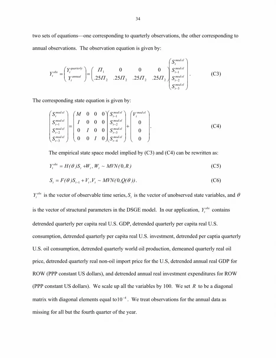
34

two sets of equations—one corresponding to quarterly observations, the other corresponding to

annual observations. The observation equation is given by:

⎟⎟⎟⎟⎟

⎠

⎞

⎜⎜⎜⎜⎜

⎝

⎛

⎟⎟⎠

⎞⎜⎜⎝

⎛=⎟⎟

⎠

⎞⎜⎜⎝

⎛=

−

−

−

elmodt

elmodt

elmodt

elmodt

annualt

quarterlytobs

t

SSSS

....YY

Y

3

2

1

2222

1

25252525000ΠΠΠΠ

Π . (C3)

The corresponding state equation is given by:

⎟⎟⎟⎟⎟

⎠

⎞

⎜⎜⎜⎜⎜

⎝

⎛

+

⎟⎟⎟⎟⎟

⎠

⎞

⎜⎜⎜⎜⎜

⎝

⎛

⎟⎟⎟⎟⎟

⎠

⎞

⎜⎜⎜⎜⎜

⎝

⎛

=

⎟⎟⎟⎟⎟

⎠

⎞

⎜⎜⎜⎜⎜

⎝

⎛

−

−

−

−

−

−

−

000

000000000000

4

3

2

1

3

2

1

elmodt

elmodt

elmodt

elmodt

elmodt

elmodt

elmodt

elmodt

elmodt V

SSSS

II

IM

SSSS

. (C4)

The empirical state space model implied by (C3) and (C4) can be rewritten as:

(C5) )R,(MVN~W,WS)(HY tttobs

t 0+= θ

))(Q,(MVN~V,VS)(FS tttt θθ 01 += − . (C6)

obstY is the vector of observable time series, is the vector of unobserved state variables, and tS θ

is the vector of structural parameters in the DSGE model. In our application, contains

detrended quarterly per capita real U.S. GDP, detrended quarterly per capita real U.S.

consumption, detrended quarterly per capita real U.S. investment, detrended per captia quarterly

U.S. oil consumption, detrended quarterly world oil production, demeaned quarterly real oil

price, detrended quarterly real non-oil import price for the U.S, detrended annual real GDP for

ROW (PPP constant US dollars), and detrended annual real investment expenditures for ROW

(PPP constant US dollars). We scale up all the variables by 100. We set

obstY

R to be a diagonal

matrix with diagonal elements equal to . We treat observations for the annual data as

missing for all but the fourth quarter of the year.

410 −

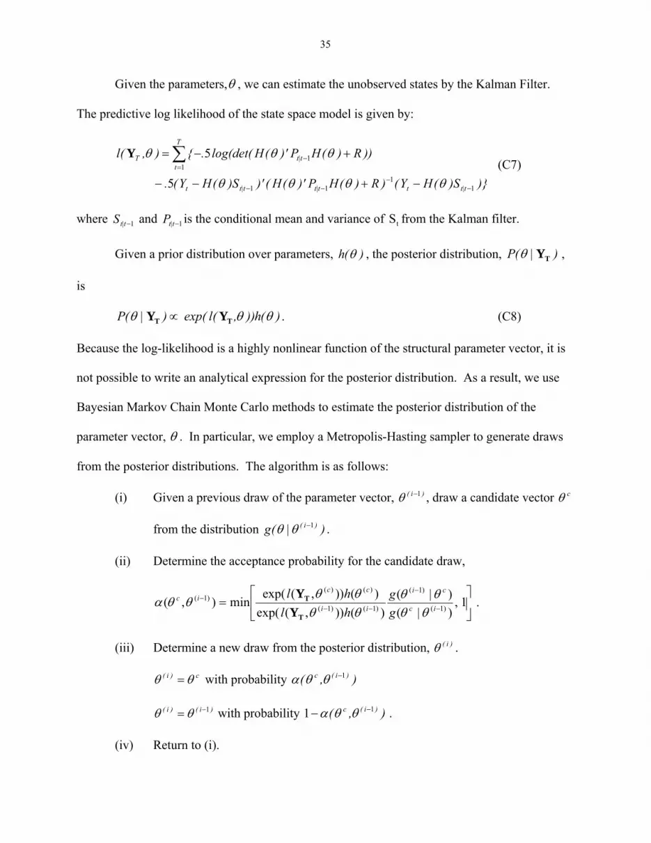
35

Given the parameters,θ , we can estimate the unobserved states by the Kalman Filter.

The predictive log likelihood of the state space model is given by:

(C7) )}S)(HY()R)(HP)'(H()'S)(HY(.

))R)(HP)'(Hlog(det(.{),(l

t|ttt|tt|tt

T

tt|tT

11

11

11

5

5

−−

−−

=−

−+−−

+−= ∑θθθθ

θθθY

where and is the conditional mean and variance of from the Kalman filter. 1−t|tS 1−t|tP tS

Given a prior distribution over parameters, )(h θ , the posterior distribution, )|(P TYθ ,

is

)(h)),(lexp()|(P θθθ TT YY ∝ . (C8)

Because the log-likelihood is a highly nonlinear function of the structural parameter vector, it is

not possible to write an analytical expression for the posterior distribution. As a result, we use

Bayesian Markov Chain Monte Carlo methods to estimate the posterior distribution of the

parameter vector, θ . In particular, we employ a Metropolis-Hasting sampler to generate draws

from the posterior distributions. The algorithm is as follows:

(i) Given a previous draw of the parameter vector, )i( 1−θ , draw a candidate vector

from the distribution )| .

cθ

(g )i( 1−θθ

(ii) Determine the acceptance probability for the candidate draw,

⎥⎦

⎤⎢⎣

⎡=

−

−

−−− 1,

)|()|(

)()),(exp()()),(exp(

min),( )1(

)1(

)1()1(

)()()1(

ic

ci

ii

ccic

gg

hlhl

θθθθ

θθθθ

θθαT

T

YY

.

(iii) Determine a new draw from the posterior distribution, )i(θ .

c)i( θθ = with probability ),

)i() 1−= θ with probability ), .

( )i(c 1−θθα

i(θ ( )i(c 11 −− θθα

(iv) Return to (i).

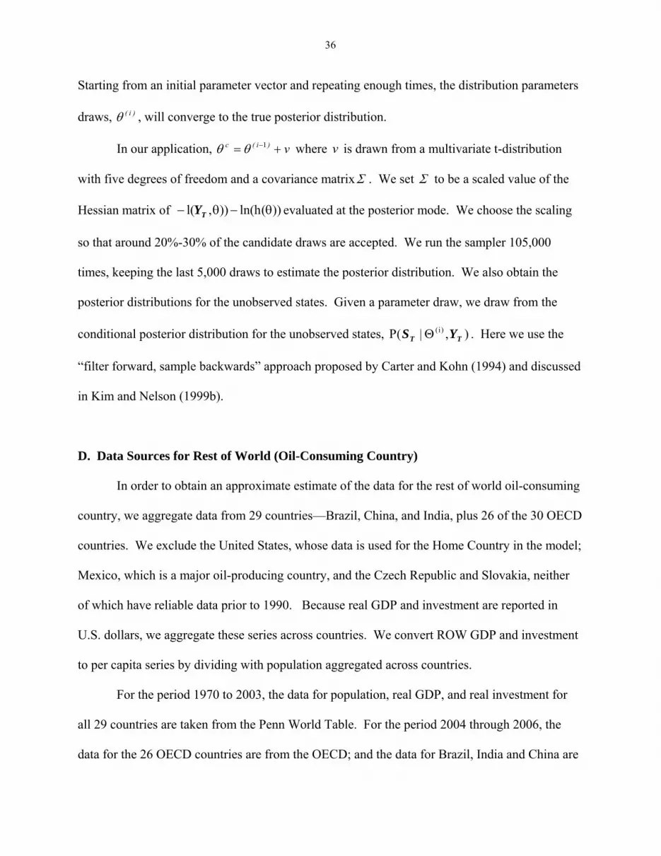
36

Starting from an initial parameter vector and repeating enough times, the distribution parameters

draws, , will converge to the true posterior distribution. )i(θ

In our application, where is drawn from a multivariate t-distribution

with five degrees of freedom and a covariance matrix

v)i(c += −1θθ v

Σ . We set Σ to be a scaled value of the

Hessian matrix of ))(hln()),(l θ−θ− TY evaluated at the posterior mode. We choose the scaling

so that around 20%-30% of the candidate draws are accepted. We run the sampler 105,000

times, keeping the last 5,000 draws to estimate the posterior distribution. We also obtain the

posterior distributions for the unobserved states. Given a parameter draw, we draw from the

conditional posterior distribution for the unobserved states, . Here we use the

“filter forward, sample backwards” approach proposed by Carter and Kohn (1994) and discussed

in Kim and Nelson (1999b).

),|(P )i(TT YS Θ

D. Data Sources for Rest of World (Oil-Consuming Country)

In order to obtain an approximate estimate of the data for the rest of world oil-consuming

country, we aggregate data from 29 countries—Brazil, China, and India, plus 26 of the 30 OECD

countries. We exclude the United States, whose data is used for the Home Country in the model;

Mexico, which is a major oil-producing country, and the Czech Republic and Slovakia, neither

of which have reliable data prior to 1990. Because real GDP and investment are reported in

U.S. dollars, we aggregate these series across countries. We convert ROW GDP and investment

to per capita series by dividing with population aggregated across countries.

For the period 1970 to 2003, the data for population, real GDP, and real investment for

all 29 countries are taken from the Penn World Table. For the period 2004 through 2006, the

data for the 26 OECD countries are from the OECD; and the data for Brazil, India and China are

37

from Haver Analytics. The data from 2004 to 2006 were spliced to the earlier data in 2003,

country by country, and then aggregated to obtain per capita measures of ROW output and

investment.

38

References: Alquist, Ron and Lutz Kilian (2007), “What Do We Learn from the Price of Crude Oil Futures?”

CEPR Discussion Papers 6548, University of Michigan. Backus, David K. and Mario J. Crucini (2000), “Oil Prices and the Terms of Trade,” Journal of

International Economics 50: 185–213. Backus, David K., Patrick J. Kehoe and Finn E. Kydland (1992), “International Real Business

Cycles,” Journal of Political Economy 100(4): 745-75. Backus, David K., Patrick J. Kehoe and Finn E. Kydland, (1994), “Dynamics of the Trade

Balance and the Terms of Trade: the J-curve?” American Economic Review 84(1): 84–103.

Balke, Nathan S., Stephen P. Brown and Mine K. Yücel (2002), “Oil Price Shocks and the U.S. Economy: Where Does the Asymmetry Originate?” The Energy Journal 23(3): 27-52 (Third Quarter).

Barsky, Robert, and Lutz Killian (2001), “Do We Really Know that Oil Caused the Great Stagflation? A Monetary Alternative,” NBER Macroeconomics Annual 2001, (May): 137-183.

Barsky, Robert, and Lutz Killian (2004), “Oil and the Macroeconomy since the 1970s,” Journal of Economic Perspectives, 18(4): 115-134 (Fall).

Bernanke, Ben S. (2004), “The Great Moderation,” speech at the meetings of the Eastern Economic Association (February).

Bernanke, Ben S., Mark Gertler, and Mark Watson (1997), “Systematic Monetary Policy and the Effects of Oil Price Shocks,” Brookings Papers on Economics Activity 1997(1): 91-142.

Blanchard, Olivier and J. Gali (2007), “The Macroeconomic Effects of Oil Price Shocks: Why are the 2000s so Different from the 1970s?” Massachusetts Institute of Technology, Department of Economics, Working Paper 07-21 (August).

Blanchard, O, and C. Kahn (1980), “The Solution of Linear Difference Equations under Rational Expectations,” Econometrica, 48: 1305-1310.

Blanchard, Olivier and John Simon (2001), “The Long and Large Decline in U.S. Output Volatility,” Brookings Papers on Economic Activity (1): 135–64.

Bodenstein, Martin, Christopher J. Erceg and Luca Guerrieri (2007), “Oil Shocks and External Adjustment,” Board of Governors of the Federal Reserve System, International Finance Discussion Paper Number 897 (June).

Bohi, Douglas R. (1989), Energy Price Shocks and Macroeconomic Performance, Resources for the Future, Washington, D.C.

Bohi, Douglas R. (1991), “On the Macroeconomic Effects of Energy Price Shocks,” Resources and Energy 13(2):145-62.

Boivin, Jean and Marc P. Giannoni (2006), “Has Monetary Policy Become More Effective?” Review of Economics and Statistics 88: 445–62 (August).

Brown, Stephen P. A. and Mine K. Yücel (1999), “Oil Prices and U.S. Aggregate Economic Activity: A Question of Neutrality,” Economic and Financial Review, Federal Reserve Bank of Dallas (Second Quarter).

Bruno, Michael R. and Jeffrey Sachs (1981), “Supply versus Demand Approaches to the Problem of Stagflation,” in Macroeconomic Policies for Growth and Stability, edited by H. Giersch, Tubingen, J. C. B. Mohr.

39

Bruno, Michael R. and Jeffrey Sachs (1985), Economics of Worldwide Stagflation. Cambridge, Mass.:Harvard University Press.

Burbidge, J and A. Harrison (1984), “Testing for the Effects of Oil-Price Rises Using Vector Autoregression,” International Economic Review, 25:459-484.

Carter, C.K. and P. Kohn (1994), “On Gibbs Sampling for State Space Models,” Biometrica 81, 541-553.

Chari, V.V., Patrick Kehoe, and Ellen McGrattan (2007), “Business Cycle Accounting,” Econometrica, 75(3): 781-836.

Darby, Michael R. (1982), “The Price of Oil and World Inflation and Recession,” American Economic Review, 72:738-751.

Davis, Steven J. and John Haltiwanger (2001), “Sectoral Job Creation and Destruction Responses to Oil Price Changes and Other Shocks,” Journal of Monetary Economics (December).

Elekdag, Sukru and Douglas Laxton (2007), “Understanding the Link Between Oil Prices and the Economy,” Box 1.1 in IMF World Economic Outlook.

Ferderer, J. Peter (1996), “Oil Price Volatility and the Macroeconomy: A Solution to the Asymmetry Puzzle,” Journal of Macroeconomics 18:1-16.

Geweke, J. (1999), “Using Simulation Methods for Bayesian Econometric Models: Inference, Development, and Communication,” Econometric Reviews 18, 1-126.

Gisser, M. and T. H. Goodwin (1986), “Crude Oil and the Macroeconomy: Tests of Some Popular Notions,” Journal of Money, Credit and Banking, 18:95-103.

Greenwood, Jeremy and Yorukoglu, Mehmet (1997). “1974,” Carnegie-Rochester Conference Series on Public Policy 46:49-95.

Hall, Robert E. (1997), “Macroeconomic Fluctuations and the Allocation of Time,” Journal of Labor Economics, 15(1): S223-S250.

Hamilton, James D. (1983), “Oil and the Macroeconomy since World War II,” Journal of Political Economy 91(2): 228-48.

Hamilton, James D. (1996), “This is What Happened to the Oil Price Macroeconomy Relationship,” Journal of Monetary Economics 38(2): 215-20 (October).

Hamilton, James D. (2003), “What Is an Oil Shock?” Journal of Econometrics 113: 363-98. Hamilton, James D. and Ana Maria Herrera (2004), “Oil Shocks and Aggregate Macroeconomic

Behavior: The Role of Monetary Policy,” Journal of Money, Credit, Banking 36(2), 265-86.

Herrera, Ana María and Elena Pesavento (forthcoming), “Oil Price Shocks, Systematic Monetary Policy and the ‘Great Moderation’,” Macroeconomic Dynamics.

Hickman, Bert, Hillard Huntington and James Sweeney, eds. (1987), Macroeconomic Impacts of Energy Shocks, Amsterdam: North-Holland.

Hooker, Mark A. (1996), “What Happened to the Oil Price Macroeconomy Relationship?” Journal of Monetary Economics, 38(2): 195-213 (October).

Hooker, Mark A. (2002), “Are Oil Shocks Inflationary? Asymmetric and Nonlinear Specifications versus Changes in Regime,” Journal of Money, Credit and Banking 34(2): 540-561.

Huntington, Hillard (2003), “Energy Disruptions, Interfirm Price Effects and the Aggregate Economy,” Energy Economics 25 (2), 119-136.

Huntington, Hillard G. (2005), Macroeconomic Consequences of Higher Oil Prices, Energy Modeling Forum Special Report 9, Stanford University, Stanford, California, August.

40

Jones, Donald W., Paul N. Leiby and Inja K. Paik (2004), “Oil Price Shocks and the Macroeconomy: What Has Been Learned Since 1996?” The Energy Journal, 25 (2).

Kahn, James A., Margaret M. McConnell and Gabriel Perez-Quiros (2002), “On the Causes of the Increased Stability of the U.S. Economy,” Economic Policy Review, Federal Reserve Bank of New York (May):183–202.

Kilian, Lutz (2008), “Exogenous Oil Supply Shocks: How Big Are They and How Much Do They Matter for the U.S. Economy?” Review of Economics and Statistics, 90(2): 216-240 (May).

Kilian, Lutz (2007), “Not All Oil Price Shocks Are Alike: Disentangling Demand and Supply Shocks in the Crude Oil Market,” Working Paper, University of Michigan.

Kim, Chang-Jin and Charles Nelson (1999a), “Has the U.S. Economy Become More Stable? A Bayesian Approach Based on a Markov-Switching Model of the Business Cycle,” Review of Economics and Statistics 81: 608-16 (November).

Kim, Chang-Jin and Charles Nelson (1999b), State Space Models with Regime Switching, MIT Press, Cambridge.

Kim, In-Moo and Prakash Loungani (1992), “The Role of Energy in Real Business Cycle Models, Journal of Monetary Economics 29: 173–189.

King, Robert. G., Charles I. Plosser and Sergio T. Rebelo (1988), “Production, Growth, and Business Cycles: I. The Basic Neoclassical Model, Journal of Monetary Economics 21: 195–232.

Lubik, T. and F. Schorfheide (2004), “Testing for Indeterminacy: An Application to U.S. Monetary Policy,” American Economic Review, 94(1): 190-217.

McConnell, Margaret M. and Gabriel Perez-Quiros (2000), “Output Fluctuations in the United States: What Has Changed Since the Early 1980s?” American Economic Review 90: 1464-76 (December)

Mork, Knut Anton and Robert E. Hall (1980), “Energy Prices, Inflation, and Recession, 1974-1975,” The Energy Journal, 1(3):31-63.

Nordhaus, William D. (2004). “Retrospective on the Postwar Productivity Slowdown,” Cowles Foundation Discussion Paper # 1494.

Pierce, James L. and Jared J. Enzler (1974), “The Effects of External Inflationary Shocks,” Brookings Papers on Economic Activity, 1:13-61.

Rasche, R.H. and J.A. Tatom (1977), “The Effects of the New Energy Regime on Economic Capacity, Production and Prices,” Economic Review, Federal Reserve Bank of St. Louis, 59(4):2-12.

Rotemberg, Julio and Michael Woodford (1996), “Imperfect Competition and the Effects of Energy Price Increases on Economic Activity,” Journal of Money, Credit and Banking 28(4): 549-577.

Samaniego, Roberto M. (2006). “Organizational Capital, Technology Adoption and the Productivity Slowdown,” Journal of Monetary Economics, 53:1555-1569.

Segal, Paul (2007), “Why Do Oil Price Shocks No Longer Shock?” Oxford Institute for Energy Studies Working Paper.

Smets, F. and R. Wouters (2007), “Shocks and Frictions in U.S. Business Cycles: A Bayesian DSGE Approach,” American Economic Review, 97(3): 586-606.

Stock, James H. and Mark W. Watson (2003), “Has the Business Cycle Changed? Evidence and Explanations,” paper presented at the Federal Reserve Bank of Kansas City symposium on Monetary Policy and Uncertainty, Jackson Hole, Wyoming (August).

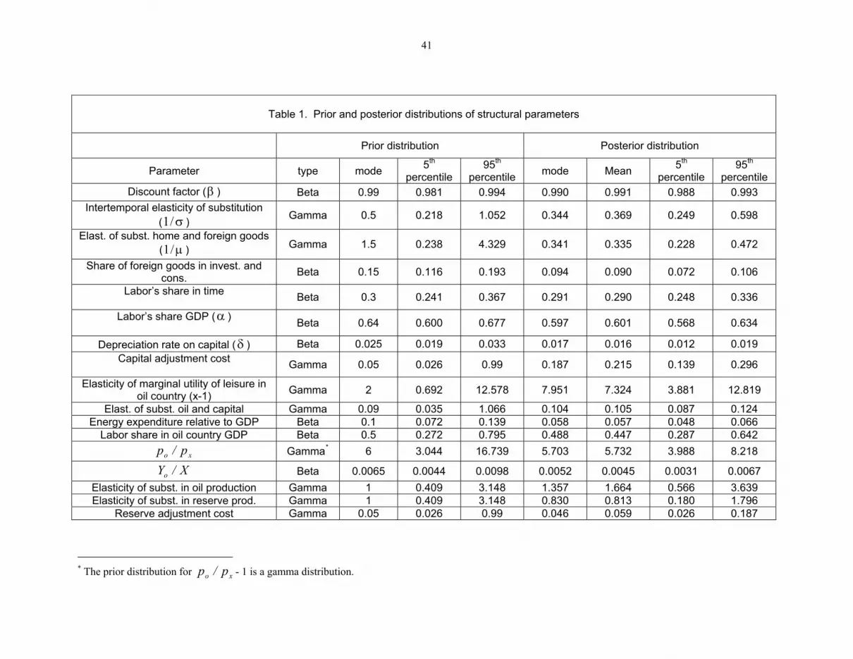
41

Table 1. Prior and posterior distributions of structural parameters

Prior distribution Posterior distribution

Parameter type mode 5th percentile

95th percentile mode Mean 5th

percentile 95th

percentile Discount factor ( ) β Beta 0.99 0.981 0.994 0.990 0.991 0.988 0.993

Intertemporal elasticity of substitution ( σ/1 ) Gamma 0.5 0.218 1.052 0.344 0.369 0.249 0.598

Elast. of subst. home and foreign goods ( μ/1 ) Gamma 1.5 0.238 4.329 0.341 0.335 0.228 0.472

Share of foreign goods in invest. and cons. Beta 0.15 0.116 0.193 0.094 0.090 0.072 0.106

Labor’s share in time Beta 0.3 0.241 0.367 0.291 0.290 0.248 0.336

Labor’s share GDP ( ) α Beta 0.64 0.600 0.677 0.597 0.601 0.568 0.634

Depreciation rate on capital ( ) δ Beta 0.025 0.019 0.033 0.017 0.016 0.012 0.019 Capital adjustment cost

Gamma 0.05 0.026 0.99 0.187 0.215 0.139 0.296

Elasticity of marginal utility of leisure in oil country (x-1) Gamma 2 0.692 12.578 7.951 7.324 3.881 12.819

Elast. of subst. oil and capital Gamma 0.09 0.035 1.066 0.104 0.105 0.087 0.124 Energy expenditure relative to GDP Beta 0.1 0.072 0.139 0.058 0.057 0.048 0.066

Labor share in oil country GDP Beta 0.5 0.272 0.795 0.488 0.447 0.287 0.642

xo p/p Gamma* 6 3.044 16.739 5.703 5.732 3.988 8.218

X/Yo Beta 0.0065 0.0044 0.0098 0.0052 0.0045 0.0031 0.0067 Elasticity of subst. in oil production Gamma 1 0.409 3.148 1.357 1.664 0.566 3.639 Elasticity of subst. in reserve prod. Gamma 1 0.409 3.148 0.830 0.813 0.180 1.796

Reserve adjustment cost Gamma 0.05 0.026 0.99 0.046 0.059 0.026 0.187

* The prior distribution for - 1 is a gamma distribution. xo p/p

42

Table 2. Prior and posterior distributions of parameters of exogenous driving forces

Prior distribution Posterior distribution

AR(1) coefficient type mode 5th percentile

95th percentile mode Mean 5th

percentile 95th

percentile US total factor productivity Beta 0.70 0.112 0.942 0.847 0.872 0.806 0.931

ROW total factor productivity Beta 0.70 0.112 0.942 0.981 0.983 0.972 0.990 Spillover in total factor productivity Normal 0.088 0.006 0.170 0.029 0.022 0.006 0.039

Oil production shock Beta 0.70 0.112 0.942 0.890 0.903 0.867 0.932 Oil reserve shock Beta 0.70 0.112 0.942 0.980 0.978 0.956 0.994 US labor wedge Beta 0.70 0.112 0.942 0.998 0.998 0.993 0.999

ROW labor wedge Beta 0.70 0.112 0.942 0.994 0.996 0.989 0.999 US oil wedge Beta 0.70 0.112 0.942 0.891 0.906 0.879 0.933

ROW oil wedge Beta 0.70 0.112 0.942 0.732 0.750 0.654 0.831 US investment shock Beta 0.70 0.112 0.942 0.874 0.876 0.767 0.960

ROW investment shock Beta 0.70 0.112 0.942 0.989 0.994 0.982 0.999

Standard deviation of innovations US total factor productivity Gamma 0.10 0.172 9.180 0.518 0.529 0.527 0.589

ROW total factor productivity Gamma 0.10 0.172 9.180 0.981 0.969 0.830 1.140 Corr(US TFP, ROW TFP) Beta†

0.258 -0.240 0.630 0.427 0.421 0.273 0.553 Oil production shock Gamma 0.10 0.172 9.180 2.937 3.019 2.394 3.595

Oil reserve shock Gamma 0.10 0.172 9.180 2.995 3.632 1.845 5.362 US labor wedge Gamma 0.10 0.172 9.180 0.882 0.881 0.785 0.976

ROW labor wedge Gamma 0.10 0.172 9.180 2.238 2.159 1.839 2.470 US oil wedge Gamma 0.10 0.172 9.180 16.665 16.743 14.486 19.311

ROW oil wedge Gamma 0.10 0.172 9.180 33.435 34.212 28.699 40.243 US investment shock Gamma 0.10 0.172 9.180 0.154 0.158 0.075 0.257

ROW investment shock Gamma 0.10 0.172 9.180 0.037 0.030 0.021 0.041

† The prior distribution for (Corr(US TFP,ROW TFP)+1)/2 is a beta distribution.

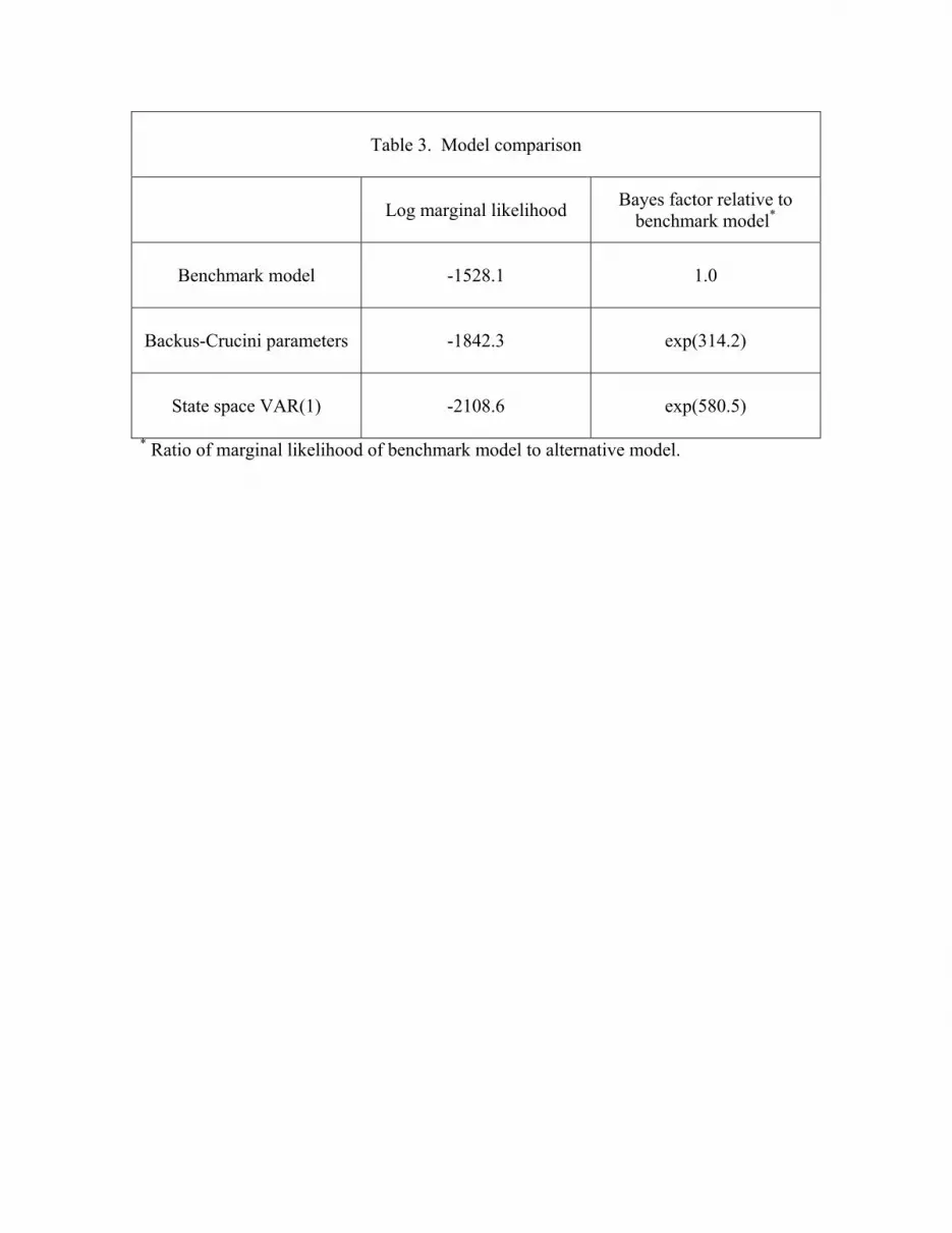
Table 3. Model comparison

Log marginal likelihood

Bayes factor relative to benchmark model*

Benchmark model

-1528.1 1.0

Backus-Crucini parameters

-1842.3 exp(314.2)

State space VAR(1)

-2108.6 exp(580.5)

* Ratio of marginal likelihood of benchmark model to alternative model.

44

0

30

60

90

120

150

48 51 54 57 60 63 66 69 72 75 78 81 84 87 90 93 96 99 02 05

Index, 1982=100

Figure 1Oil Price Shocks and U.S. Recessions

45

-15

-10

-5

0

5

10

15

1971 1974 1977 1980 1983 1986 1989 1992 1995 1998 2001 2004 2007-0.07

-0.05

-0.03

-0.01

0.01

0.03

0.05

0.07

Oil Price

Quarterly Change

Figure 2Oil Prices and U.S. GDP

GDP Cyclical Component

Deviation

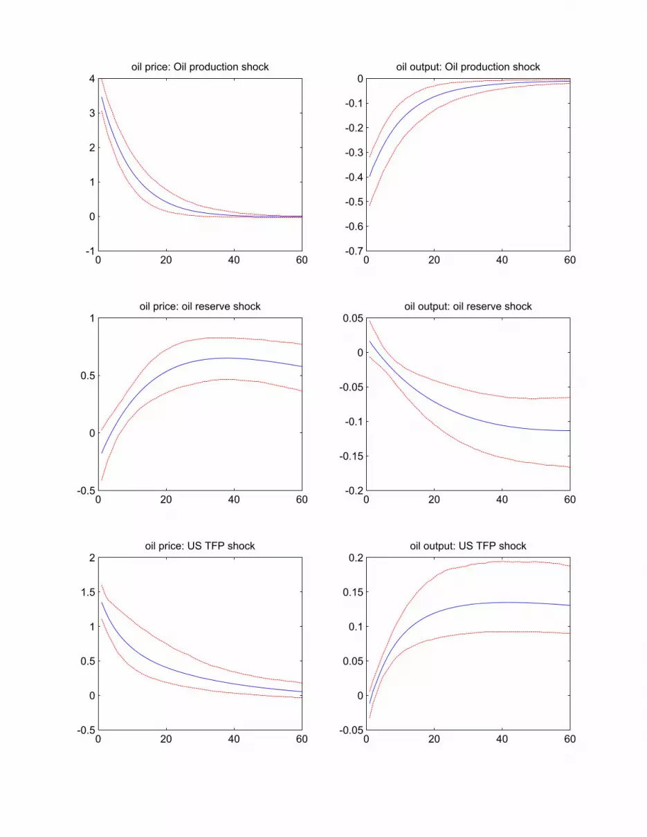
0 20 40 60-1

0

1

2

3

4oil price: Oil production shock

0 20 40 60-0.7

-0.6

-0.5

-0.4

-0.3

-0.2

-0.1

0oil output: Oil production shock

0 20 40 60-0.5

0

0.5

1oil price: oil reserve shock

0 20 40 60-0.2

-0.15

-0.1

-0.05

0

0.05oil output: oil reserve shock

0 20 40 60-0.5

0

0.5

1

1.5

2oil price: US TFP shock

0 20 40 60-0.05

0

0.05

0.1

0.15

0.2oil output: US TFP shock

0 20 40 60-0.3

-0.2

-0.1

0

0.1

0.2

0.3

0.4

0.5oil price: US labor wedge shock

0 20 40 60-0.2

-0.15

-0.1

-0.05

0oil output: US labor wedge shock

0 20 40 60-0.25

-0.2

-0.15

-0.1

-0.05

0oil price: US Oil wedge shock

0 20 40 60-0.05

-0.04

-0.03

-0.02

-0.01

0oil output: US Oil wedge shock

0 20 40 600

2

4

6

8

10

12oil price: US Investment shock

0 20 40 60-1

-0.5

0

0.5

1

1.5

2

2.5

3oil output: US Investment shock

0 20 40 60-0.035

-0.03

-0.025

-0.02

-0.015

-0.01

-0.005

0output: Oil prod shock

0 20 40 60-0.07

-0.06

-0.05

-0.04

-0.03

-0.02

-0.01

0output: Oil reserve shock

0 20 40 600

0.2

0.4

0.6

0.8

1

1.2

1.4output: US TFP

0 20 40 600.05

0.1

0.15

0.2

0.25

0.3

0.35

0.4output: ROW TFP

0 20 40 60-0.65

-0.6

-0.55

-0.5

-0.45

-0.4

-0.35

-0.3output: US labor wedge

0 20 40 60-0.035

-0.03

-0.025

-0.02

-0.015

-0.01

-0.005

0

0.005output: ROW labor wedge

0 20 40 60-0.01

-0.008

-0.006

-0.004

-0.002

0output: US oil wedge

0 20 40 60-2

0

2

4

6

8

10

12

14x 10-4 output: ROW oil wedge

0 20 40 60-4

-3

-2

-1

0

1

2output: US Investment shock

0 20 40 60-0.2

0

0.2

0.4

0.6

0.8output: ROW Investment shock

1970 1980 1990 2000 2010-100

-50

0

50

100oil supply shocks

1970 1980 1990 2000 2010-100

-50

0

50

100oil demand shocks

1970 1980 1990 2000 2010-100

-50

0

50

100US oil demand shocks

1970 1980 1990 2000 2010-100

-50

0

50

100ROW oil demand shocks

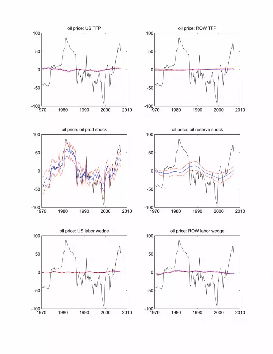
1970 1980 1990 2000 2010-100

-50

0

50

100oil price: US TFP

1970 1980 1990 2000 2010-100

-50

0

50

100oil price: ROW TFP

1970 1980 1990 2000 2010-100

-50

0

50

100oil price: oil prod shock

1970 1980 1990 2000 2010-100

-50

0

50

100oil price: oil reserve shock

1970 1980 1990 2000 2010-100

-50

0

50

100oil price: US labor wedge

1970 1980 1990 2000 2010-100

-50

0

50

100oil price: ROW labor wedge

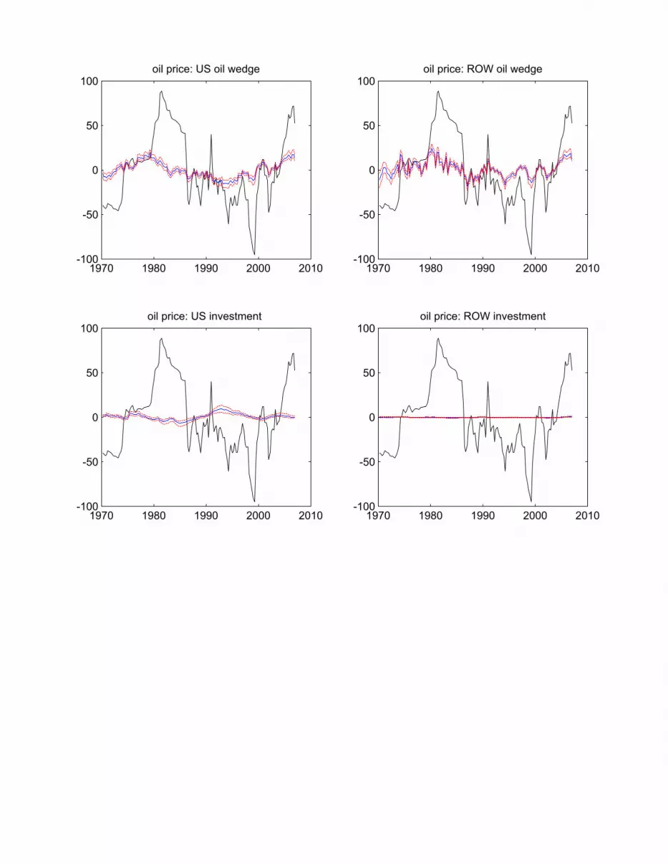
1970 1980 1990 2000 2010-100

-50

0

50

100oil price: US oil wedge

1970 1980 1990 2000 2010-100

-50

0

50

100oil price: ROW oil wedge

1970 1980 1990 2000 2010-100

-50

0

50

100oil price: US investment

1970 1980 1990 2000 2010-100

-50

0

50

100oil price: ROW investment

1970 1980 1990 2000 2010-10

-5

0

5

10US GDP: oil supply shocks

1970 1980 1990 2000 2010-10

-5

0

5

10US GDP: US shocks

1970 1980 1990 2000 2010-10

-5

0

5

10US GDP: ROW shocks

1970 1980 1990 2000 2010-10

-5

0

5

10US GDP: US TFP

1970 1980 1990 2000 2010-10

-5

0

5

10US GDP: ROW TFP

1970 1980 1990 2000 2010-10

-5

0

5

10US GDP: oil prod shock

1970 1980 1990 2000 2010-10

-5

0

5

10US GDP: oil reserve shock

1970 1980 1990 2000 2010-10

-5

0

5

10US GDP: US labor wedge

1970 1980 1990 2000 2010-10

-5

0

5

10US GDP: ROW labor wedge

1970 1980 1990 2000 2010-10

-5

0

5

10US GDP: US oil wedge

1970 1980 1990 2000 2010-10

-5

0

5

10US GDP: ROW oil wedge

1970 1980 1990 2000 2010-10

-5

0

5

10US GDP: US investment

1970 1980 1990 2000 2010-10

-5

0

5

10US GDP: ROW investment

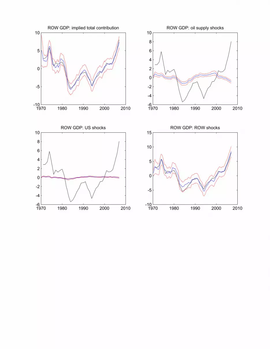
1970 1980 1990 2000 2010-10

-5

0

5

10ROW GDP: implied total contribution

1970 1980 1990 2000 2010-6

-4

-2

0

2

4

6

8

10ROW GDP: oil supply shocks

1970 1980 1990 2000 2010-6

-4

-2

0

2

4

6

8

10ROW GDP: US shocks

1970 1980 1990 2000 2010-10

-5

0

5

10

15ROW GDP: ROW shocks