Embed Size (px)
Citation preview

arX
iv:0
710.
5566
v2 [
mat
h.O
A]
21
May
200
9
AN INFINITE DIMENSIONAL SCHUR-HORN THEOREM AND
MAJORIZATION THEORY WITH APPLICATIONS TO OPERATOR IDEALS
VICTOR KAFTAL AND GARY WEISS
Abstract. The main result of this paper is the extension of the Schur-Horn Theorem to infinite sequences:For two nonincreasing nonsummable sequences ξ and η that converge to 0, there exists a positive compactoperator A with eigenvalue list η and diagonal sequence ξ if and only if
Pnj=1
ξj ≤Pn
j=1ηj for every n if
and only if ξ = Qη for some orthostochastic matrix Q. When ξ and η are summable, requiring additionallyequality of their infinite series obtains the same conclusion, extending a theorem by Arveson and Kadison.Our proof depends on the construction and analysis of an infinite product of T-transform matrices. Furtherresults on majorization for infinite sequences providing “intermediate” sequences generalize known resultsfrom the finite case. Majorization properties and invariance under various classes of stochastic matrices arethen used to characterize arithmetic mean closed operator ideals.
1. Introduction
The Schur-Horn Theorem characterizes the diagonals of a (finite) selfadjoint matrix in terms of sequencemajorization, that is, the order relation ξ 4 η for ξ, η ∈ RN given by
∑nj=1 ξ∗j ≤∑n
j=1 η∗j for 1 ≤ n ≤ N and
∑Nj=1 ξj =
∑Nj=1 ηj , where ξ∗, η∗ denote the monotone nonincreasing rearrangement of ξ, η. The theory of
majorization arose during the early part of the 20th century from a number of apparently unrelated topics:wealth distribution (Lorenz [27]), inequalities involving convex functions (Hardy, Littlewood and Polya [12]),convex combinations of permutation matrices (Birkhoff [4]), and more central to our interests herein, doublystochastic matrices and the relation between eigenvalue lists and diagonals of selfadjoint matrices:
Theorem 1.1. Let ξ, η ∈ RN .(i) Hardy, Littlewood and Polya Theorem [12]. ξ 4 η if and only ξ = Pη for some doubly stochasticmatrix P .
(ii) Horn Theorem [13, Theorem 4]. ξ 4 η if and only if ξ = Qη for some orthostochastic matrix Q, i.e.,the Schur-square of an orthogonal matrix (Qij = (Uij)
2 ∀ i, j for some unitary matrix U with real entries).(iii) Schur-Horn Theorem [35],[13]. Given a selfadjoint N ×N matrix A having eigenvalue list η, there isa basis in which A has diagonal entries ξ if and only if ξ 4 η.
The sufficiency part of the Schur-Horn Theorem is due to Schur and the necessity follows immediatelyfrom the Horn Theorem. The main goal of this paper is to extend to infinite dimension the Horn Theoremand hence the Schur-Horn Theorem.
The notion of majorization extends seamlessly to infinite sequences that admit a monotone nonincreasingrearrangement and in this paper, to avoid always having to pass to monotone rearrangements, we will focuson sequences decreasing monotonically to 0 and will denote by c*
o their positive cone and by (ℓ1)∗ the subconeof summable decreasing sequences. (We note explicitly that c*
o and (ℓ1)∗ do not mean herein the duals of co
and ℓ1.) Even for finite sequences, the terminology and notations describing majorization vary considerablyin the literature. In this paper, we will use the following notations:
Definition 1.2. For ξ, η ∈ c*o we say that
• η majorizes ξ (ξ ≺ η) if∑n
j=1 ξj ≤∑nj=1 ηj for every n ∈ N;
• η strongly majorizes ξ (ξ 4 η) if ξ ≺ η and lim∑n
j=1(ηj − ξj) = 0;
• η block majorizes ξ (ξ ≺b η) if ξ ≺ η and∑nk
j=1 ξj =∑nk
j=1 ηj for some sequence N ∋ nk ↑ ∞.
For ξ, η ∈ (ℓ1)∗ we say that
Date: May 22, 2009.1991 Mathematics Subject Classification. Primary: 15A51, 47L20 .Key words and phrases. Schur-Horn theorem, majorization, stochastic matrices, operator ideals.
1

2 VICTOR KAFTAL AND GARY WEISS
• η majorizes at infinity ξ (ξ ≺∞ η) if∑∞
j=n ξj ≤∑∞j=n ηj for every n ∈ N;
• η strongly majorizes at infinity ξ (ξ 4∞ η) if ξ ≺∞ η and∑∞
j=1 ξj =∑∞
j=1 ηj.
If ξ, η ∈ c+o
(resp. (ℓ1)+), then we say that any of the above relations hold for ξ and η if they hold for theirmonotone rearrangements ξ∗ and η∗.
For nonsummable monotone decreasing sequences, the condition lim∑n
j=1(ηj − ξj) = 0 retains many of
the key properties of ”equality at the end” for finite and for summable sequences (e.g., see Section 7) and itwill prove crucial for our extension of the Schur-Horn Theorem.
Majorization at infinity, aka “tail majorization,” was first introduced and studied for finite sequences andappears in [1], [24], [7], [37] among others. It holds particular relevance for this paper as it provides thenatural characterization of the notion of arithmetic mean closure at infinity for operator ideals contained inthe trace class (see Theorem 8.3 and [18]-[22]).
Block-majorization is both a natural way to bring the results of finite majorization theory to bear oninfinite sequences and it also arises naturally in Sections 4,7, and 8. See in particular the proof of ourextension of a known finite intermediate sequence result:
• If ξ, η ∈ c*o and ξ ≺ η, then there are ζ, ρ ∈ c*
o for which ξ 4 ζ ≤ η and ξ ≤ ρ 4 η (Theorem 7.4).
and of a similar result for majorization at infinity (Theorem 7.7).In 1964, in two papers that are not nearly as well-known as they deserve and with two almost disjoint
approaches, Markus [28] and Gohberg and Markus [10] found infinite dimensional versions of the Hardy,Littlewood and Polya Theorem 1.1(i) and an extension to the summable case of the Horn Theorem [13,Theorem 4], (Theorem 1.1 (ii)). More recently, Arveson and Kadison obtained other characterizations in [3]using still different methods.
If ξ, η ∈ c*o, then
ξ ≺ η ⇐⇒ ξ = Qη for some substochastic Q (Q row-stochastic if ξn > 0 ∀n) [28, Lemma 3.1](1)
ξ ≺ η ⇐⇒ ξ = Qη with Qij = |Wij |2, for some co-isometry W [10, Proposition III, pg 205]
ξ ≺ η ⇐⇒ ξ = Qη with Qij = |Lij |2, for some contraction L [3, Theorem 4.2]
If ξ, η ∈ (ℓ1)+, then
ξ 4 η ⇐⇒ ξ = Qη with Qij = |Uij |2, for some unitary U [10, Theorem 1](2)
ξ 4 η ⇐⇒ ξ = Qη with Qij = |Wij |2, for some isometry W [3, Theorem 4.1]
By reformulating matricially the proof of Markus’s [28, Lemma 3.1] and slightly tightening it (see Remark3.8), we can identify a sequence of orthogonal matrices underlying the construction. An analysis of theirproperties and infinite products permits us to obtain:
• If ξ, η ∈ c*o, ξn > 0 ∀n, and ξ ≺ η, then there is a canonical co-isometry with real entries W (ξ, η)
for which ξ = Q(ξ, η)η with Q(ξ, η)ij = (W (ξ, η)ij)2 (Theorem 3.7).
• If ξ, η ∈ c*o, then ξ 4 η ⇐⇒ ξ = Qη with Qij = |Uij |2 for some orthogonal matrix U (Theorem 3.9).
Not surprisingly, this construction applied to finite sequences provides another proof of the (finite) HornTheorem 1.1(ii).
The canonical matrix Q(ξ, η) is obtained as an infinite product of T-transforms (see Section 3 for details)and is therefore completely determined by the sequence {mk, tk} where mk is the matrix size and 0 < tk ≤ 1is the “convex coefficient” of the k-th transform. In Section 4 we further analyze this double sequence and,more precisely the set {tk | mk = 1}, in order to link properties of the majorization ξ ≺ η with properties ofthe corresponding canonical matrix Q(ξ, η):
• ξ 4 η if and only if Q(ξ, η) is orthostochastic (i.e., if W (ξ, η) is orthogonal) if and only if∑{tk | mk = 1} = ∞ (Theorem 4.7).
• ξ ≺b η if and only Q(ξ, η) is the direct sum of finite orthostochastic matrices if and only ifcard{k | tk = mk = 1} = ∞ (Proposition 4.4).
Notice that if ξ, η ∈ c*o and ξ = Qη for some orthostochastic matrix Q, then by (1) it follows that ξ ≺ η, but
in general it does not follow that ξ 4 η. In fact, a main results of this paper is:
• If ξ, η ∈ c*o, ξ 6∈ (ℓ1)∗ and ξ ≺ η, then there is an orthostochastic matrix Q for which ξ = Qη
(Theorem 5.3).

INFINITE DIMENSIONAL SCHUR-HORN THEOREM 3
Section 5 is devoted to the proof of this theorem by showing that a pair of c*o-sequences ξ ≺ η with ξ non-
summable and ξ 64 η can be decomposed into “mutually orthogonal” pairs of infinite subsequences for whichstrong majorization holds (Lemmas 5.1-5.2) and then invoking Theorem 3.9 to obtain an orthostochasticmatrix for each pair and direct summing them. Together, Theorems 3.9 and 5.3 provide the following infinitedimensional extension of the Horn Theorem (Remark 5.4):
• If ξ, η ∈ c*o then ξ = Qη for some orthostochastic matrix Q ⇐⇒
{
ξ ≺ η if ξ 6∈ ℓ1
ξ 4 η if ξ ∈ ℓ1.
To apply the Horn Theorem to positive compact operators, notice first that the eigenvalue list with multi-plicity (which is the sequence s(A) of s-numbers of A ∈ K(H)+) “ignores” the nullspace of A (e.g., see (32))and hence it characterizes the partial isometry orbit V(A) := {V AV ∗ | V partial isometry, V ∗V A = A} of Arather than, as in the finite rank case, the unitary orbit U(A) of A. Then if we fix an orthonormal basis of theHilbert space H and denote by E the canonical conditional expectation on the corresponding atomic masaD (i.e., the operation of “taking the main diagonal”), we obtain the following infinite dimension extensionof the Schur-Horn Theorem for positive compact operators:
• E(V(A)) =
{
{B ∈ D ∩ K(H)+ | s(B) ≺ s(A)} \ L1 if Tr(A) = ∞{B ∈ D ∩ K(H)+ | s(B) 4 s(A)} if Tr(A) < ∞.
(Proposition 6.4 ).
If A has finite rank, then U(A) = V(A) and if A ∈ K(H)+ has dense range, i.e., RA = I then
• E(U(A)) =
{
{B ∈ D ∩ K(H)+ | s(B) ≺ s(A), RB = I} \ L1 if Tr(A) = ∞{B ∈ D ∩ K(H)+ | s(B) 4 s(A), RB = I} if Tr(A) < ∞.
(Proposition 6.6 )
For positive compact operators with infinite rank some sufficient conditions and some necessary conditionsfor membership in E(U(A)) are presented in Propositions 6.6 and 6.10. Our work extends some of the resultsof Gohberg and Marcus in [10] and Arveson and Kadison in [3]. There are only limited overlaps betweenour paper and those by A. Neumann [33] and by Antezana, Massey, Ruiz, and Stojanoff [2] as these authorscharacterize the closures of the expectation of the unitary orbit of a selfadjoint not necessarily compactoperator while we do not take closures. The connections with these three papers are further discussed inSection 6 where we also answer a couple of questions of Neumann. The following, in the case of sequencesξ, η ∈ c*
o. compares these different results to Proposition 6.4 .
If ξ 6∈ (ℓ1)∗, then ξ ≺ η ⇔ diag ξ ∈
E(U(diag η))||.||
([33, Theorem 3.13])
E{L diag ηL∗ | L ∈ B(H)1} ([3, Theorem 4.2])
E(U(diag η)) (Proposition 6.4 )
If ξ ∈ (ℓ1)∗, then ξ 4 η ⇔ diag ξ ∈
E(U(diag η))||.||1
([2, Proposition 3.13])
E(U(diag η)||.||1
) ([3, Theorem 4.2])
E(U(diag η)) ([10, Theorem 1], Proposition 6.4 )
Finally, in Section 8 we apply results on majorization for infinite sequences to operator ideals (two-sidedideals of B(H)). We characterize arithmetic mean closed ideals and arithmetic mean at infinity closed ideals(see Section 8 for the definitions) in terms of the diagonals of their positive elements (Theorems 8.1, 8.3)and in terms of invariance under the action of various classes of (sub) stochastic matrices (Corollary 8.7,Theorem 8.9). This paper began as part of a long-term project investigating arithmetic mean ideals andarithmetic mean at infinity ideals [18]-[22].
2. Notations and preliminaries on stochastic matrices
Let c*o denote the cone of nonnegative monotone nonincreasing sequences converging to 0 and (ℓ1)∗ the
cone of nonnegative monotone nonincreasing summable sequences. (Again, notice that c*o and (ℓ1)∗ here do
not denote the duals of co and ℓ1.) If ξ ∈ (co)+, denote by ξ∗ its nonincreasing rearrangement.
For every sequence ξ = < ξ1, ξ2, . . . > and every n = 0, 1, . . . , denote by ξ(n) the truncated sequenceξ(n) = < ξn+1, ξn+2, . . . > and by ξχ[1, n] the sequence < ξ1, ξ2, . . . , ξn, 0, . . . >. We will of course identifyξχ[1, n] with a vector in Rn and conversely, embed Rn into co by completing finite sequences with infinitelymany zeros.

4 VICTOR KAFTAL AND GARY WEISS
When applying the majorization notations of Definition 1.2 to finite sequences, we caution the reader
again that what we call majorization (ξ ≺ η, i.e.,∑k
1 ξj ≤ ∑k1 ηj for all 1 ≤ k ≤ n) is often called weak
majorization, and what we call strong majorization (ξ 4 η, i.e., ξ ≺ η with∑n
j=1 ξj =∑n
j=1 ηj) is mostlycalled majorization, although with no universal agreement about notations or even about the direction ofthe inequalities (see [14, Remark, page 198]). For the theory of majorization of finite sequences we refer thereader to Marshall and Olkin [29].
Immediate consequences of Definition 1.2 are:
If ξ, η ∈ c*o, then ξ ≺b η ⇒ ξ 4 η ⇒ ξ ≺ η.(3)
If ξ, η ∈ (ℓ1)∗, then ξ ≺ η and∞∑
j=1
ξj =∞∑
j=1
ηj ⇔ ξ 4 η ⇔ η 4∞ ξ.
Once we have fixed an orthonormal basis {ek} for a complex separable infinite-dimensional Hilbert spaceH , i.e., once we have identified H with ℓ2, we will also identify infinite matrices with operators and willuse these terms interchangeably. E.g., when we apply a Hilbert space operator to a sequence in c*
o, whatwe mean is that we apply the corresponding matrix to that sequence – which for substochastic matricesis always possible (e.g., see Remark 2.2). Also, for typographical reasons we are not going to distinguishbetween row and column vectors, e.g., if P is a matrix, we shall write P < ξ1, ξ2, . . . > in lieu the moreprecise P < ξ1, ξ2, . . . >T.
K(H) denotes the ideal of compact operators and L1 the trace class ideal, with tr denoting the usualtrace. Given a compact operator A ∈ K(H), the sequence s(A) ∈ c*
o of its s-numbers (singular numbers)consists of the eigenvalues of (A∗A)1/2 in monotone order, with repetition according to multiplicity, and withinfinitely many zeros added in case A has finite rank. In particular, if A ≥ 0 has infinite rank, then s(A) isprecisely the “eigenvalue list” of A.
Given a sequence ρ ∈ ℓ∞, we denote by diag ρ the diagonal matrix having ρ as its main diagonal. Givenan operator A ∈ B(H), we denote by E(A) the diagonal matrix having as diagonal the main diagonal of A,i.e., E : B(H) → D is the normal faithful and trace preserving conditional expectation from B(H) onto themasa D of diagonal operators.
Stochastic matrices play a key role in majorization theory of finite sequences (e.g, see Theorem 1.1(i)). Asimilar but necessarily more complex role is played in the case of infinite sequences.
Definition 2.1. A matrix P with nonnegative entries is called
• substochastic if its row and column sums are bounded by 1;• column-stochastic if it is substochastic with column sums equal to 1;• row-stochastic if it is substochastic with row sums equal to 1;• doubly stochastic if it is both column and row-stochastic;• block stochastic if it is the direct sum of finite doubly stochastic matrices.
Remark 2.2.
(i) Contrary to the finite case a (square) matrix can be column-stochastic without being row stochastic andvice versa.
(ii) We can apply a substochastic matrix P to any sequence ρ ∈ ℓ∞, where by Pρ we just mean the sequence<∑∞
j=1 Pijρj >.
(iii) If ρ ∈ co and P is substochastic, then Pρ ∈ co.(iv) By Schur’s test (e.g., see [11, Problem 45]) substochastic matrices viewed as Hilbert space operators arecontractions.
An important class of stochastic matrices is the one obtained as “Schur-squares” of contractions. To bemore precise, we should call them the Schur product of a contraction by its complex conjugate matrix, but inmost cases we consider only matrices with real entries. The Schur product is also called Hadamard productor entrywise product. The relevance of these stochastic matrices is clear from the following well-knownlemma whose verification is straightforward.
Lemma 2.3. Let ξ, η ∈ c*o and let Qij = |Lij |2 for all i, j for some contraction L ∈ B(H). Then
diag ξ = E(L diag η L∗) if and only if ξ = Qη.

INFINITE DIMENSIONAL SCHUR-HORN THEOREM 5
Lemma 2.4. Let Qij = |Lij |2 for all i, j for some contraction L ∈ B(H). Then(i) Q is substochastic.(ii) Q is column-stochastic if and only if L is an isometry.(ii′) Q is row-stochastic if and only if L is a co-isometry.
Proof. Notice first that
(4)
∞∑
j=1
Qij =
∞∑
j=1
LijL∗ji = ||L∗ei||2 ≤ 1 for every i,
and similarly
(5)
∞∑
i=1
Qij = ||Lej||2 ≤ 1 for every j.
(i) Immediate from (4) and (5).(ii) Sufficiency is immediate from (i) and (5). Conversely, assume that Q is column-stochastic and hence||Lej|| = 1 for all j by (5). Then (L∗Lej, ej) = 1 for all j and thus E(I − L∗L) = 0. Since E is faithful andI − L∗L ≥ 0 because L is a contraction, it follows that L∗L = I.
(ii′) Apply (ii) to L∗. �
Definition 2.5. If Qij = |Lij |2 for some contraction L, then we say that Q is isometry stochastic (resp. co-isometry stochastic, unistochastic, orthostochastic) if L is an isometry (resp. co-isometry, unitary, orthogonalmatrix, i.e., a unitary matrix with real entries). If L is the direct sum of finite unitary (resp. orthogonal)matrices, we say that Q is block unistochastic (resp. block orthostochastic.)
Remark 2.6.
(i) The terminology “orthostochastic” goes back at least to Horn (cf. [13]). When the entries of the unitarymatrix are not necessarily real, its Schur-square is called unitary stochastic in [29], Pythagorean in [17,Section 4], and orthostochastic in [15], although unistochastic appears to be the more common term now.
(ii) Q can be the Schur-square of different contractions, e.g., Qij = |L(1)ij |2 = |L(2)
ij |2; but L(1) is an isometry,
a co-isometry, a unitary if and only if so is L(2), respectively. Of course, L(1) may have real entries, whileL(2) does not.
(iii) L does not need to be a contraction for Q to be doubly stochastic, e.g., consider the 4 × 4 matrix L withconstant entries 1
2 .(iv) As remarked by Horn [13], every 2 × 2 doubly stochastic matrix is necessarily orthostochastic but
1
2
1 1 01 0 10 1 1
is doubly stochastic but not unistochastic (see [29, p. 39] for more examples).(v) Let P be a matrix and Π be a permutation matrix. Then ΠP is substochastic (resp. row-stochastic,column-stochastic, isometry stochastic, co-isometry stochastic, unistochastic, orthostochastic) precisely whenP is. However, permutations do not preserve block stochasticity.
An immediate consequence of Theorem 1.1(i) and (ii) is that
if ξ, η ∈ c*o, then ξ ≺b η ⇔ ξ = Qη for a block orthostochastic matrix Q(6)
⇔ ξ = Qη for a block stochastic matrix Q.
Another simple application of the Horn Theorem, which we will need in Theorem 3.9, is to the case whenη is a sequence with finite support. This result generalizes [17, Theorem 13] (see also [2, Theorem 4.7].)
Lemma 2.7. If ξ, η ∈ c*o , ξ 4 η, and η has finite support, then ξ = Qη for some orthostochastic matrix Q.
Proof. The case when η = 0 being trivial, let n be the largest integer for which ηn > 0. If n = 1, then
let U be an orthogonal matrix that has as its first column the unit vector(√
ξ1
η1,√
ξ2
η1,√
ξ3
η1, · · ·
)T
and let
Qij := U2ij . Then Qη = ξ. In the case that n > 1, we have
∑∞j=1 ξj =
∑nj=1 ηj >
∑n−1j=1 ηj . Let m

6 VICTOR KAFTAL AND GARY WEISS
be the index for which∑m−1
j=1 ξj ≤ ∑n−1j=1 ηj <
∑mj=1 ξj and let α :=
∑mj=1 ξj −∑n−1
j=1 ηj . Then m ≥ n,
0 < α = ηn −∑∞j=m+1 ξj ≤ ηn and
< ξ1, ξ2, . . . , ξm > 4 < η1, η2, . . . , ηn−1, α, 0, . . . , 0 > .
By applying the Horn Theorem (see Theorem 1.1 (ii)) to the above two vectors of (Rm)+, we find an m×morthostochastic matrix Qo for which
Qo < η1, η2, . . . , ηn−1, α, 0, . . . , 0 > = < ξ1, ξ2, . . . , ξm >
and let Uo be an orthogonal matrix for which Qoij = (Uo
ij)2. In particular, the first n columns U1, U2, . . . , Un of
Uo are orthonormal. Denote by Q1, Q2, . . . , Qn their Schur-squares, i.e., the first n columns of Qo. Thereforethe ℓ2 vectors
U1
00...
,
U2
00...
, . . . ,
Un−1
00...
,
√αηn
Un√
ξm+1
ηn√ξm+2
ηn
...
are also orthonormal. Complete them to an orthonormal basis of ℓ2 with real entry vectors and denote byU the orthogonal matrix having as columns these vectors and by Q the orthostochastic matrix Qij = U2
ij .Then
Q =
Q1 . . . Qn−1αηn
Qn ∗ ∗ . . .
0 . . . 0 ξm+1
ηn∗ ∗ . . .
0 . . . 0 ξm+2
ηn∗ ∗ . . .
......
......
......
...
and hence
Qη =
(Q1 . . . Qn−1
αηn
Qn
)
η1
η2
...ηn
0 . . . 0 ξm+1
ηn.
0 . . . 0 ξm+2
ηn
......
......
η1
η2
...ηn
=
(Q1 . . . Qn−1 Qn
)
η1
η2
...ηn−1
α
ξm+1
ξm+2
...
= ξ.
�
The following lemma is a key “bridge” between properties of majorization and properties of stochasticmatrices.
Lemma 2.8. If P is a substochastic matrix for which limn
∑ni=1(ηi − (Pη)i) = 0 for some η ∈ c*
o withηn > 0 for all n, then P is column-stochastic.
Proof.n∑
i=1
(ηi − (Pη)i) =
n∑
j=1
(1 −
n∑
i=1
Pij
)(ηj − ηn) +
∞∑
j=n+1
n∑
i=1
Pij(ηn − ηj) +(n −
n∑
i=1
∞∑
j=1
Pij
)ηn
≥ (1 −n∑
i=1
Pij)(ηj − ηn) ≥ 0 for all n ≥ j.
Thus for all j,
0 = limn
n∑
i=1
(ηi − (Pη)i) ≥ limn
(1 −n∑
i=1
Pij)(ηj − ηn) = (1 −∞∑
i=1
Pij)ηj ≥ 0,

INFINITE DIMENSIONAL SCHUR-HORN THEOREM 7
hence∑∞
i=1 Pij = 0. �
Remark 2.9.
(i) The first line of the proof is based on Ostrowski’s decomposition [34] and shows that∑n
i=1(ηi − (Pη)i) ≥ 0whether Pη is monotone or not. It was used by Markus to prove that Pη ≺ η in [28, Lemma 3.1].
(ii) If Pη is monotone, then the condition Pη 4 η is equivalent to limn
∑ni=1(ηi − (Pη)i) = 0 and hence
implies that P is column-stochastic.(iii) In the case that ζ ∈ (ℓ1)+ and
∑∞j=1(Pζ)j =
∑∞j=1 ζj, it is immediate to verify that
∑∞=1 Pjn = 1 for every
n which ζn 6= 0. The same conclusion can be obtained by the operator theoretic argument in [3, Theorem4.1] in the case that Pij = |Lij |2 for some contraction L. For the reader’s convenience, a sketch of the
argument is that then Tr(diag ζ) = Tr(E(L diag ζ L∗)) and hence Tr(
E((diag ζ)
12 (I − L∗L)(diag ζ)
12
))
= 0
Since I − L∗L ≥ 0 and Tr and E are faithful, it follows that (diag ζ)12 (I − L∗L)(diag ζ)
12 = 0 and hence
||Len|| = 1 for every n for which ζn 6= 0.(iv) Notice that if P is a substochastic matrix for which Pη 4 η for some η ∈ c*
o with ηn > 0 for all n, P canfail to be row-stochastic as is the case for
P :=
1/2 0 0 0 . . .1/2 0 0 0 . . .0 1/2 0 0 . . .0 1/2 0 0 . . .0 0 1/2 0 . . .0 0 1/2 0 . . ....
......
......
and η any summable sequence with ηn > 0 for all n.
For summable sequences the converse of Lemma 2.8 holds.
Lemma 2.10. Let ξ, η ∈ c*o and ξ = Pη for some column-stochastic matrix P . If ξ ∈ (ℓ1)∗ (resp. η ∈ (ℓ1)∗),
then η ∈ (ℓ1)∗ (resp. ξ ∈ (ℓ1)∗) and ξ 4 η.
Proof. We know from (1) that ξ ≺ η. Moreover,
∞∑
i=1
ξi =
∞∑
i=1
(Pη)i =
∞∑
i=1
∞∑
j=1
Pijηj =
∞∑
j=1
∞∑
i=1
Pijηj =
∞∑
j=1
ηj ,
thus ξ ∈ (ℓ1)∗ if and only if η ∈ (ℓ1)∗ and ξ 4 η. �
Without the condition of summability, the implication in Lemma 2.10 can fail. In fact, the followingexample shows that it can fail even for an orthostochastic matrix as seen by modifying the matrix in Remark2.9(iv) as follows. Let ω denote the harmonic sequence, i.e., ω := < 1
n >.
Example 2.11. An orthostochastic matrix Q for which Qω 64 ω.
Proof. Partition N into two infinite strictly increasing sequence {nk} and {mk} for which
lim(∑2k
j=k+11nj
− ∑kj=1
1mj
)
> 0. For instance, this can be achieved by setting mk := (k + 1)2 and
listing N \ {mk} as {nk}.
Defining
Uij =
1√2
if i = 2k − 1 , j = nk, k ∈ N
1√2
if i = 2k − 1, j = mk, k ∈ N
1√2
if i = 2k, j = nk, k ∈ N
− 1√2
if i = 2k, j = mk, k ∈ N
0 otherwise
.

8 VICTOR KAFTAL AND GARY WEISS
it is easy to see that U is an orthogonal matrix. Let Q be the Schur-square of U , i.e., Qij := U2ij . Then a
simple computation shows that for every k ∈ N,
(Qω)2k−1 = (Qω)2k =1
2
( 1
nk+
1
mk
)
and hence (Qω)2k > (Qω)2k+1, that is, Qω is monotone nonincreasing. Moreover,
2k∑
j=1
ωj −2k∑
j=1
(Qω)j =
2k∑
j=1
1
j−
k∑
i=1
( 1
ni+
1
mi
)≥
2k∑
j=k+1
1
ni−
k∑
j=1
1
mi.
Similarly,
2k+1∑
j=1
ωj −2k+1∑
j=1
(Qω)j =
2k+1∑
j=1
1
j−
k∑
i=1
( 1
ni+
1
mi
)− 1
2(
1
nk+1+
1
mk+1)
≥2k∑
j=k+1
1
ni−
k∑
j=1
1
mi− 1
2(
1
nk+1+
1
mk+1).
Thus lim(∑n
j=1 ωj −∑n
j=1(Qω)j
)
≥ lim(∑2k
j=k+11
nj−∑k
j=11
mj
)
> 0, i.e., Qω 64 ω. �
We will see from Theorem 5.3 that for any nonsummable sequence η we can choose an orthostochastic matrixQ for which Qη = 1
2η and hence Qη 64 η.
We know of no simple condition that characterizes substochastic matrices for which Pη 4 η for all η ∈ c*o.
Notice that since Pη is not necessarily monotone, by the latter condition we mean (Pη)∗ 4 η for themonotone rearrangement (Pη)∗ of Pη. A sufficient condition is that P is block stochastic, i.e., the directsum of doubly stochastic finite matrices. A more general sufficient condition is provided by the followinglemma.
Lemma 2.12. If P is a substochastic matrix and lim (n −∑ni,j=1 Pij) = 0, then
(i) P is doubly stochastic;(ii) Pη 4 η for every η ∈ c*
o.
Proof.(i)
n −n∑
i,j=1
Pij =
n∑
i=1
(1 −n∑
j=1
Pij) ≥n∑
i=1
(1 −∞∑
j=1
Pij)
thus
0 = lim (n −n∑
i,j=1
Pij) ≥∞∑
i=1
(1 −∞∑
j=1
Pij).
Then because P is substochastic,∑∞
j=1 Pij = 1 for all i. Similarly,∑∞
i=1 Pij = 1 for all j.
(ii) Since∑n
i=1(Pη)i ≤∑n
i=1(Pη)∗i for every n,
n∑
i=1
(ηi − (Pη)∗i ) ≤n∑
i=1
(ηi − (Pη)i)
=
n∑
j=1
(1 −n∑
i=1
Pij)ηj −n∑
i=1
∞∑
j=n+1
Pijηj
≤n∑
j=1
(1 −n∑
i=1
Pij)||η||∞
= (n −n∑
i,j=1
Pij)||η||∞,
hence lim∑n
i=1(ηi − (Pη)i)∗ ≤ lim (n −∑n
i,j=1 Pij)||η||∞ = 0. Thus (Pη)∗ 4 η, i.e., by Definition 1.2,Pη 4 η.

INFINITE DIMENSIONAL SCHUR-HORN THEOREM 9
�
Remark 2.13. The condition lim (n −∑ni,j=1 Pij) = 0 is not necessary for (ii). For instance, (ii) holds
trivially for every permutation matrix Π since (Πη)∗ = η for every η, but it is easy to find a permutationmatrix Π for which lim(n −∑n
i,j=1 Πij) > 0.
3. The canonical co-isometry of a majorization
We start with some historical notes about the link between majorization and stochastic matrices.Muirhead [32] for the case of integer-valued finite sequences and then Hardy, Littlewood and Polya [12,
p. 47] for the case of real-valued finite sequences proved that for all ξ, η ∈ RN with ξ 4 η, there is a doublystochastic matrix P with ξ = Pη. P was obtained as a finite product of T-transforms, i.e. matrices of theform tI +(1− t)Π with Π a transposition and 0 ≤ t < 1. The T-transforms were chosen so to reduce at eachstep the Hamming distance (i.e., the number of positions where two sequences differ) between the sequence ξand the iterated transform of η. Notice that while individual T-transforms are orthostochastic, the productof two T-transforms can fail to be even unistochastic ([29, Chapter II, Section G]).
In 1952, Horn proved that the matrix P can be chosen to be orthostochastic by using a different methodbased on convexity arguments and a technically difficult proof [13, Theorem 4].
A proof based on properties of determinants was given a few years later by Mirsky [30, Theorem 2].After a four decade hyatus, a proof based on composition of Givens rotations (special permutations of
T-transforms) was obtained by Casazza and Leon in the Appendix of [6].More recently, Arveson and Kadison [3, Theorem 2.1] gave an elegant proof of the Horn theorem showing
that P can be chosen to be unistochastic (see also [16, Lemma 5 and Theorem 6]). Reformulating their resultin our terminology, they showed that ξ is obtained by applying to η a finite number of T-transforms andthat by properly choosing unitary matrices whose Schur-squares are those T-transforms, the Schur-squareof their product (a unistochastic matrix by definition) applied to η also yields ξ.
Another recent proof was obtained by Kornelson and Larson [25, Theorem 2]. More precisely, they provedthe equivalent statement that every positive finite rank operator B with eigenvalue list η can be decomposed
as the linear combination B =∑k
j=1 ξjPj of rank-one projections (not required to be mutually orthogonal)
with the given monotone nonincreasing coefficient sequence ξ := < ξ1, ξ2, . . . ξk, 0 . . . >, if and only if (in ournotations) ξ 4 η.
This link between majorization and stochastic matrices was partially extended to the infinite case byMarkus in [28, Lemma 3.1] (see (1)) and the Schur-Horn Theorem was extended to summable sequencesby Gohberg and Markus in [10, Lemma 1] (see (2)) based on [10, Theorem 1]. The latter proof dependedcrucially on the summability of the sequence, so we focus on the former proof.
At the core of Markus’s proof, although he did not employ this terminology nor exhibit explicitly thematrices, is the construction, for every ξ, η ∈ c*
o with ξ ≺ η, of an infinite sequence of permutations ofT-transforms whose product is a substochastic matrix Q for which ξ = Qη. Furthermore, a remark in hisproof states that when ξn > 0 for all n, the matrix Q is row-stochastic. In this section we revisit andslightly tighten the Markus construction for the case when ξn > 0 for all n (see Remark 3.8) and provethat it provides a co-isometry stochastic matrix (Theorem 3.7) and in the strong majorization case, anorthostochastic matrix (Theorems 3.9, 4.7). Not surprisingly, this construction restricted to finite sequencesyields another proof of the Horn Theorem (Remark 4.3)
For every integer m ≥ 1 and 0 < t ≤ 1, define the m + 1 × m + 1 orthogonal matrix
(7) V (m, t) :=
0 0 . . . 0√
t −√
1 − t1 0 . . . 0 0 00 1 . . . 0 0 0...
......
......
...0 0 . . . 1 0 0
0 0 . . . 0√
1 − t√
t
.
Notice that the Schur-square of the matrix V (m, t) is the product of the permutation matrix Π1 that sends< 1, 2, . . . , m, m + 1 > to < m, 1, 2, . . . , m − 1, m + 1 > and of the T-transform tI + (1 − t)Π2 where Π2 isthe transposition that interchanges m and m + 1.

10 VICTOR KAFTAL AND GARY WEISS
Given a sequence {mk, tk} where mk ∈ N and 0 < tk ≤ 1, define for every n ∈ N
(8) W (n) :=(In−1 ⊕ V (mn, tn) ⊕ I∞
)(In−1 ⊕ V (mn, tn) ⊕ I∞
)· · ·(I1 ⊕ V (m2, t2) ⊕ I∞
)(V (m1, t1) ⊕ I∞
)
where In denotes the n× n identity matrix for 1 ≤ n ≤ ∞ and I0 is simply dropped. Define also R(n) to bethe Schur-square of V (mn, tn) ⊕ I∞, and let
(9) Q(n) :=(In−1 ⊕ R(n)
)(In−2 ⊕ R(n−1)
)· · ·(I1 ⊕ R(2)
)R(1).
Being a product of orthogonal matrices, all W (n) are also orthogonal. Denote by Pn := In⊕ 0 the projectionon span{e1, . . . , en}.
Proposition 3.1. Let {mk, tk} be a sequence with mk ∈ N and 0 < tk ≤ 1. Then(i) The sequence of operators W (n) converges in the weak operator topology to a co-isometry W ({mk, tk})and PnW ({mk, tk}) = PnW (n) for every n. The convergence is in the strong operator topology if and only ifW ({mk, tk}) is orthogonal.
(ii) The sequence of operators Q(n) converges in the weak operator topology to a row-stochastic operatorQ({mk, tk}) and PnQ({mk, tk}) = PnQ(n) for every n.
Proof.(i) From (8) we have for all integers j > n,
W (j) = (Ij−1 ⊕ V (mj , tj) ⊕ I∞) · · · (In ⊕ V (mn+1, tn+1) ⊕ I∞)W (n)
and hence
(10) PnW (j) = PnW (n) for all j ≥ n.
As a consequence,((W (j) − W (i))x, y
)=((W (j) − W (i))x, P⊥
n y)
for all x, y ∈ H and i, j ≥ n. Thus the
sequence of orthogonal matrices {W (j)} is weakly Cauchy and hence converges weakly to a contractionW ({mk, tk}) with real entries. Set W := W ({mk, tk}). From (10), it follows that PnW = PnW (n) for all n,
that is, the first n rows of the matrix W (n) stabilize: Wij = W(n)ij for all n, j and all i ≤ n. Therefore
WW ∗ = s-lim PnWW ∗Pn = s-limPnW (n)(W (n))∗Pn = s-limPn = I,
i.e., W is a co-isometry. Since ||(W −W (n))x||2 → ||x||2−||Wx||2 for all x ∈ H , the sequence W (n) convergesstrongly to W if and only if W is orthogonal.
(ii) Same proof. �
Remark 3.2. Proposition 3.1 holds even if we allow tk = 0. However, in order to obtain the uniqueness ofthe sequence {mk, tk} in the construction in Theorem 3.7, we will have to assume there that tk > 0 for allk. In addition, this assumption will simplify some of the proofs.
A case where it is simple to find the form of W ({mk, tk}) and Q({mk, tk}) is when mk = 1 for all k.
Example 3.3.
W ({1, tk}) =
√t1 −√
1 − t1 0 0 . . .√
t2(1 − t1)√
t2t1 −√1 − t2 0 . . .
√
t3(1 − t2)(1 − t1)√
t3(1 − t2)t1√
t3t2 −√1 − t3 . . .
......
......
...√
tk∏k−1
i=1 (1 − ti)
√
tkt1∏k−1
i=2 (1 − ti)
√
tkt2∏k−1
i=3 (1 − ti)
√
tkt3∏k−1
i=4 (1 − ti) . . ....
......
......

INFINITE DIMENSIONAL SCHUR-HORN THEOREM 11
Q({1, tk}) =
t1 1 − t1 0 0 . . .t2(1 − t1) t2t1 1 − t2 0 . . .
t3(1 − t2)(1 − t1) t3(1 − t2)t1 t3t2 1 − t3 . . ....
......
......
tk∏k−1
i=1 (1 − ti) tkt1∏k−1
i=2 (1 − ti) tkt2∏k−1
i=3 (1 − ti) tkt3∏k−1
i=4 (1 − ti) . . ....
......
......
We see in this case that Q({1, tk}) is the Schur-square of W ({1, tk}). For the general case we first statea couple of elementary lemmas leaving their proof to the reader.
Lemma 3.4. Let A and B be two bounded matrices with the property that for every i, j there is at most oneindex k for which AikBkj 6= 0 and let A′ and B′ be the Schur-square of A and B respectively. Then A′B′ isthe Schur-square of AB. If furthermore A and B are orthogonal (resp. unitary) then A′B′ is orthostochastic(resp. unistochastic). In particular, if Q is orthostochastic (resp. unistochastic) and Π is a permutation,then ΠQ is orthostochastic (resp. unistochastic).
Next, we consider a simple case where this sufficient condition is satisfied.
Lemma 3.5. Let A and B be bounded matrices, let n ∈ N, and assume that for every j there is at most oneindex i > n for which Bij 6= 0.
(i) For every i and j there is at most one index k for which (In ⊕ A)ikBkj 6= 0.(ii) If for every j there is at most one index i > 1 (resp. i > 0) for which Aij 6= 0, then for every j there isat most one index i > n + 1 (resp. i > n) for which
((In ⊕ A)B
)
ij6= 0.
(iii) Let A(n) be a sequence of bounded matrices for which for every n and j, A(n)ij 6= 0 for at most oneindex i > 1 and let Q =
(In−1 ⊕A(n)
)(In−2 ⊕A(n− 1)
)· · ·(I1 ⊕ A(2)
)A(1). Then for every j, Qij 6= 0 for
at most one index i > n.
Given a sequence {mk, tk} where mk ∈ N and 0 < tk ≤ 1, then for every n, j, at most one of the entries
W(n)ij for i > n is nonzero.
Proposition 3.6. Let {mk, tk} be a sequence with mk ∈ N and 0 < tk ≤ 1 and let W (n) and Q(n) be as in(8) and (9). Then
(i) Q(n) is the Schur-square of W (n) for every n and for every n and j there is at most one index i > n for
which Q(n)ij 6= 0.
(ii) Q({mk, tk}) is the Schur-square of W ({mk, tk}).Proof.
(i) We reason by induction. Q(1) is by definition the Schur-square of W (1). Assume that Q(n) is the Schur-square of W (n). Now W (n+1) =
(In ⊕ V (mn+1, tn+1) ⊕ I∞
)W (n). Since for every factor V (mk, tk) ⊕ I∞
and every j there is at most one index i > 1 for which(V (mk, tk) ⊕ I∞
)
ij6= 0, it follows from Lemma
3.5(iii) that for every n and j, W(n)ij 6= 0 for at most one index i > n. Thus by Lemma 3.5(i), for every i
and j, (In ⊕ V (mn+1, tn+1) ⊕ I∞)
ikW
(n)kj 6= 0 for at most one index k. But then, the product of Q(n+1) =
(In ⊕ R(n+1)
)Q(n) of the Schur-square of In ⊕ V (mn+1, tn+1) ⊕ I∞ by the Schur-square of W (n) coincides
by Lemma 3.4 with the Schur-square of W (n+1) =(In ⊕ V (mn+1, tn+1) ⊕ I∞
)W (n).
(ii) Obvious since the first n rows of W ({mk, tk}) (resp. Q({mk, tk})) coincide with the first n rows of W (n)
(resp. Q(n).) �
To every majorization ξ ≺ η with ξn > 0 for all n, the following construction associates a sequence {mk, tk}with mk ∈ N and 0 < tk ≤ 1 and hence associates the corresponding co-isometry W (ξ, η) := W ({mk, tk}).Theorem 3.7. Let ξ, η ∈ c*
o with ξn > 0 for every n. If ξ ≺ η, then there is a canonical co-isometry W (ξ, η)with real entries whose Schur-square Q(ξ, η) satisfies ξ = Q(ξ, η)η.

12 VICTOR KAFTAL AND GARY WEISS
Proof. We construct the following sequence {mk, tk} where mk ∈ N and 0 < tk ≤ 1. Set ρ(0) := η andchoose m1 ∈ N for which ηm1+1 < ξ1 ≤ ηm1 . Since ξ ≺ η and hence ξ1 ≤ η1, and since ξ1 > 0 and ηj → 0,such an integer exists and by the monotonicity of η, it is unique. Express ξ1 as a convex combinationof ηm1 and ηm1+1, that is, choose t1 for which ξ1 = t1ηm1 + (1 − t1)ηm1+1. Thus 0 < t1 ≤ 1 and alsot1 is uniquely determined. Set δ1 := (1 − t1)ηm1 + t1ηm1+1 and hence δ1 = ηm1 + ηm1+1 − ξ1. Definethe sequence ρ(1) := < η1, η2, . . . , ηm1−1, δ1, ηm1+2, ηm1+3, . . . > where if m1 = 1, then the first entry ofρ(1) is δ1. Since ηm1+2 ≤ ηm1+1 ≤ δ1 < ηm1 ≤ ηm1−1, we see that ρ(1) is monotone nonincreasing and
ρ(1) ≤ η. Let R(1) be the Schur-square of V (m1, t1) ⊕ I∞, i.e., R(1)ij =
((V (m1, t1) ⊕ I∞
)
ij
)2for all i, j.
Then R(1)η = < ξ1, ρ(1)1, ρ(1)2, . . . > . Moreover,
(11) ξ(1) ≺ ρ(1).
(Recall the notation ξ(1) := < ξ2, ξ3, . . . >.) Indeed, for every 1 ≤ n < m1,
n∑
j=1
(ρ(1)j − ξ(1)j ) =
n∑
j=1
ηj −n+1∑
j=2
ξj =
n∑
j=1
(ηj − ξj) + ξ1 − ξn+1 ≥ 0,
and for every n ≥ m1
n∑
j=1
(ρ(1)j − ξ(1)j ) =
m1−1∑
j=1
ηj + δ1 +
n+1∑
j=m1+2
ηj −n+1∑
j=2
ξj =
n+1∑
j=1
(ηj − ξj) ≥ 0.
Repeat the construction applying it to the pair ξ(1) ≺ ρ(1), and so on. By the assumption that ξk > 0 for allk, the process can be iterated providing an infinite sequence of pairs {mk, tk} with mk ∈ N and 0 < tk ≤ 1and from these, of sequences ρ(k) and scalars δk satisfying for all k the relations:
ρ(k − 1)mk+1 < ξk ≤ ρ(k − 1)mk, ξk = tkρ(k − 1)mk
+ (1 − tk)ρ(k − 1)mk+1,(12)
δk := (1 − tk)ρ(k − 1)mk+ tkρ(k − 1)mk+1 = ρ(k − 1)mk
+ ρ(k − 1)mk+1 − ξk,(13)
ρ(k) := < ρ(k − 1)1, . . . , ρ(k − 1)mk−1, δk, ρ(k − 1)mk+2, . . . >, i.e.,
ρ(k)j =
ρ(k − 1)j for all j < mk
δk for j = mk
ρ(k − 1)j+1 for all j > mk,
(14)
ξ(k) ≺ ρ(k), η = ρ(0) ≥ ρ(1) ≥ ρ(2) ≥ · · · ,(15)
n∑
j=1
(ρ(k)j − ξ(k)j ) =
n+1∑
j=1
(ρ(k − 1)j − ξ(k−1)j ) for all n ≥ mk.(16)
Let R(n) be the Schur-square of V (mn, tn) ⊕ I∞, and let Q(n) := (In−1 ⊕ R(n)) · · · (I1 ⊕ R(2))R(1) as in (9).Then for all n,
(17) R(n)ρ(n − 1) = < ξn, ρ(n)1, ρ(n)2, . . . >, Q(n)η = < ξ1, ξ2, . . . , ξn, ρ(n)1, ρ(n)2, . . . >
Let
W (ξ, η) := W ({mk, tk}) and Q(ξ, η) := Q({mk, tk}).Then by Propositions 3.1 and 3.6, W (ξ, η) is a co-isometry and Q(ξ, η) is its Schur-square. Finally, by
Remark 2.2, Q(ξ, η)η is defined and is a sequence in co. In fact, by (17),
PnQ(ξ, η)η = PnQ(n)η = < ξ1, ξ2, . . . , ξn, 0, 0, . . . >→ ξ pointwise,
and hence Q(ξ, η)η = ξ.�

INFINITE DIMENSIONAL SCHUR-HORN THEOREM 13
Remark 3.8.
(i) The construction of the sequence {mk, tk} and the associated sequence of matrices Q(n) follows the Markusconstruction in [28, Lemma 3.1]. A minor difference is that while Markus chose mk to be an index for whichηmk+1 ≤ ξk ≤ ηmk
so to treat at the same time also the case when ξ is finitely supported, here we consideronly the case of infinitely supported ξ and then request that ηmk+1 < ξk ≤ ηmk
, which makes the constructioncanonical. The main difference is that Markus’s analysis is at the level of the action of the matrices Q(n)
on η, and thus yields only that their limit Q is row-stochastic. It is by introducing the underlying matricesW (n) and analyzing their properties that we can obtain that Q is co-isometry stochastic.
(ii) As a consequence of [10, Proposition III, pg 205] obtained by Gohberg and Markus with different methods,is that if ξ ≺ η, then ξ = Qη for some co-isometry stochastic matrix Q (see Remark 6.5(ii) for more details.)
When the majorization is strong, we obtain the following extension of the Horn Theorem [13, Theorem4](see Theorem 1.1(ii)). In the nonsummable case strong majorization will not be required, as we will see inTheorem 5.3.
Theorem 3.9. If ξ, η ∈ c*o and ξ 4 η, then ξ = Qη for some orthostochastic matrix Q.
Proof. If η has finite support, then the conclusion follows from Lemma 2.7. If η has infinite support, thenξ too has infinite support. Indeed, if otherwise ξn = 0 for some n, then
∑∞j=1 ηj =
∑n−1j=1 ξj ≤ ∑n−1
j=1 ηj
which implies that ηn = 0, a contradition. But then, by Theorem 3.7, ξ = Q(ξ, η)η where Q(ξ, η) is theSchur-square of the co-isometry W (ξ, η). By Lemma 2.8 and Remark 2.9(ii), Q(ξ, η) is column-stochasticand hence by Lemma 2.4 , W (ξ, η) is also an isometry and hence unitary. Since by construction W (ξ, η) hasreal entries, it is orthogonal, hence Q(ξ, η) is orthostochastic. �
Remark 3.10.
(i) The above proof shows that if ξ 4 η and η has infinite support, then any co-isometry stochastic matrix Qfor which ξ = Qη must be unistochastic, i.e., the Schur product of a unitary matrix by its complex conjugate.
(ii) In the case when ξ 4 η and ξ has infinite support but η does not, we cannot invoke Lemma 2.8 to concludethat W (ξ, η) is orthogonal, so for simplicity’s sake, we have chosen in lieu of Q(ξ, η) the orthostochasticmatrix provided by Lemma 2.7. However, in the next section we will prove that if ξ 4 η, then Q(ξ, η) itselfis orthostochastic (Theorem 4.7).
(iii) If ξ has finite support, say {1, . . . , N}, then the construction of Theorem 3.7 can still be carried on forthe first N steps and it provides yet another proof of the Horn Theorem (see Remark 4.3).
4. Properties of the canonical matrix Q(ξ, η) of a majorization
In this section, on which the following ones do not depend, we further analyze the construction in Theorem3.7 to relate the properties of the majorization ξ ≺ η to those of the canonical co-isometry stochastic matrixQ(ξ, η) via the properties of the set {tk | mk = 1}. In the next lemmas we collect the additional neededproperties of the sequences mk, tk, δk, ρ(k), W (n), etc. that were introduced in Theorem 3.7
Lemma 4.1. Let ξ, η ∈ c*o, ξ ≺ η, and assume that ξn > 0 for all n. Then for every k ∈ N
(i) mk ≥ mk−1 − 1;(ii) ρ(k)j = ηj+k for every j > mk;
(iii) if n ≥ mk, then∑n
j=1(ρ(k)j − ξ(k)j ) =
∑n+kj=1 (ηj − ξj);
(iv) if mk = 1, then δk = ηk+1 +∑k
j=1(ηj − ξj);
(v) if tk = 1, and mk = mk−1 − 1, then tk−1 = 1;
(vi) if∑n
j=1(ηj − ξj) = 0 and∑n−1
j=1 (ηj − ξj) > 0 for some n > 1, then mn = tn = 1.
Proof.(i) Assume by contradiction that mk < mk−1 − 1, then
ξk > ρ(k − 1)mk+1 (by (12))
= ρ(k − 2)mk+1 (by (14) since mk + 1 < mk−1)
≥ ρ(k − 2)mk−1(by the monotonicity of ρ(k − 2), since mk + 1 < mk−1)
≥ ξk−1 (by (12)).
This is a contradiction because of the monotonicity of ξ.

14 VICTOR KAFTAL AND GARY WEISS
(ii) The proof is by induction on k. The property holds by (14) for k = 1 since by definition ρ(0) = η. Assumeit holds for some k and let j > mk+1. Then,
ρ(k + 1)j = ρ(k)j+1 (by (14))
= ηj+1+k (by the induction hypothesis, since by (i), j + 1 > mk.)
(iii) If n ≥ mk, then by (i), n + p ≥ mk−p for all 0 ≤ p < k. Thus iterating (16)
n∑
j=1
(ρ(k)j − ξ(k)j ) =
n+k∑
j=1
(ρ(0)j − ξ(0)j ) =
n+k∑
j=1
(ηj − ξj).
(iv) Since δk = ρ(k)1 by (14), setting n = 1 in (iii) we obtain
δk = ξk+1 +
k+1∑
j=1
(ηj − ξj) = ηk+1 +
k∑
j=1
(ηj − ξj).
(v) ξk−1 ≤ ρ(k − 2)mk−1(by (12))
≤ ρ(k − 2)mk(by the monotonicity of ρ(k − 2), since mk < mk−1)
= ρ(k − 1)mk(by (14), since mk < mk−1)
= ξk (by (12), since tk = 1)
≤ ξk−1 (by the monotonicity of ξ.)
But then, ξk−1 = ρ(k − 2)mk−1and hence by (12), tk−1 = 1.
(vi) We reason by induction on n and first prove the property for n = 2. If η1 + η2 = ξ1 + ξ2 and η1 > ξ1,then η2 < ξ2 ≤ ξ1 < η1. Thus m1 = 1, ρ(1)1 = δ1 = η1 + η2 − ξ1 = ξ2 and hence m2 = t2 = 1. Assume
now that the property (vi) holds for some n ≥ 2 for every pair of sequences and that∑n+1
j=1 (ηj − ξj) = 0 and∑n
j=1(ηj − ξj) > 0. Then ηn+1 < ξn+1 ≤ ξ1 ≤ ηm1 implies that n + 1 > m1 and from (16) we obtain that∑n
j=1(ρ(1)j − ξ(1)j ) =
∑n+1j=1 (ηj − ξj) = 0. We claim that
∑n−1j=1 (ρ(1)j − ξ
(1)j ) > 0. If n > m1, the claim holds
because
ρ(1)n = ηn+1 (by (14))
< ξn+1
= ξ(1)n (by definition)
= ρ(1)n +n−1∑
j=1
(ρ(1)j − ξ(1)j ) (since
n∑
j=1
(ρ(1)j − ξ(1)j ) = 0.)
If n = m1, i.e., ηn+1 < ξ1 ≤ ηn, then
n−1∑
j=1
(ρ(1)j − ξ(1)j ) = ξ(1)
n − ρ(1)n (sincen∑
j=1
(ρ(1)j − ξ(1)j ) = 0)
= ξn+1 − δ1 (by (14))
= ξn+1 − ηn+1 + ξ1 − ηn (by (13))
=
n−1∑
j=1
ηj −n∑
j=2
ξj (since
n+1∑
j=1
(ηj − ξj) = 0.)
Thus, if ξ1 = ηn, then∑n−1
j=1 (ρ(1)j − ξ(1)j ) = ξn+1 − ηn+1 > 0. If on the other hand ξ1 < ηn, then by
the monotonicity of η and ξ, we have∑n−1
j=1 ηj >∑n−1
j=1 ξj ≥ ∑nj=2 ξj , thus completing the proof of the
claim. Therefore the sequences ξ(1) ≺ ρ(1) satisfy the hypotheses of (vi) for n and hence, by the inductionhypothesis, satisfy the thesis of (vi). But by definition, the pair {mn, tn} for ξ(1) ≺ ρ(1) coincides with thepair {mn+1, tn+1} for ξ ≺ η, which concludes the induction proof.
�

INFINITE DIMENSIONAL SCHUR-HORN THEOREM 15
Without the assumption that∑n−1
j=1 (ηj − ξj) > 0, the conclusion of (vi) may fail: consider for instanceξ =< 1, 1, ∗, . . . > and η =< 1, 1, 1, 0, . . . > where m2 = 2.
Lemma 4.2. Let ξ, η ∈ c*o with ξn > 0 for all n and ξ ≺ η.
(i) W (n) = Pn+mnW (n)Pn+mn
+ P⊥n+mn
for every n.
(ii) If Pn commutes with W (ξ, η), then∑n
j=1(ηj − ξj) = 0.
(iii) If mn = tn = 1, then Pn commutes with W (n) and with W (ξ, η) and ρ(n) = η(n).
Proof.(i) By Lemma 4.1(i), the sizes k + mk of the matrices Ik−1 ⊕ V (mk, tk) are nondecreasing. Thus for every1 ≤ k ≤ n,
P⊥n+mn
(Ik−1 ⊕ V (mk, tk) ⊕ I∞
)=(Ik−1 ⊕ V (mk, tk) ⊕ I∞
)P⊥
n+mn= P⊥
n+mn.
By (8), P⊥n+mn
W (n) = W (n)P⊥n+mn
= P⊥n+mn
and hence the claim.(ii) If W (ξ, η) commutes with Pn, i.e., W (ξ, η)ij = 0 when 1 ≤ i ≤ n and j > n and when 1 ≤ j ≤ nand i > n, then so does its Schur-square Q(ξ, η). But then, the n × n matrix Qn := PnQ(ξ, η)Pn
∣∣PnH
is also orthostochastic. Since Q(ξ, η)η = ξ, it follows that Qn < η1, . . . , ηn >=< ξ1, . . . , ξn > and hence∑n
j=1(ηj − ξj) = 0.
(iii) By Lemma 4.1 (i), for every k, either mk−1 ≤ mk or mk−1 = mk + 1. Let j be the largest index i ≤ nfor which mi−1 ≤ mi and if there is none, set j = 1. Then mi = n + 1 − i for all j ≤ i ≤ n. By applyingrecursively Lemma 4.1(v) we obtain that ti = 1 for all j ≤ i ≤ n. But then the size of all the matricesIi−1 ⊕ V (n + 1 − i, 1) is constant and equal to n + 1, hence
W (n) =
(((In−1 ⊕ V (1, 1))(In−2 ⊕ V (2, 1)) . . . (Ij−1 ⊕ V (n + 1 − j, 1))
)
⊕ I∞
)
W (j−1)
where we set W (0) = I if j = 1. All the matrices Ii−1 ⊕ V (n + 1 − i, 1) for j ≤ i ≤ n are n + 1 × n + 1permutation matrices that leave the n + 1 position fixed and hence they commute with Pn. If j = 1, thenW (0) = I commutes trivially with Pn, while if j > 1, then mj−1 = mj = n + 1− j, hence n = j − 1 + mj−1,
and thus by (i), W (j−1) also commutes with Pn. Thus PnW (n) = W (n)Pn. As PnW (ξ, η) = PnW (n) byProposition 3.1, it follows that PnW (ξ, η)P⊥
n = 0. On the other hand, W (ξ, η) is a co-isometry and W (n) isunitary, hence
P⊥n W (ξ, η)Pn = P⊥
n W (ξ, η)(W (n))∗W (n)Pn = P⊥n W (ξ, η)(W (n))∗PnW (n)
= P⊥n W (ξ, η)W (ξ, η)∗PnW (n) = P⊥
n PnW (n) = 0
which proves that W (ξ, η) commutes with Pn. Moreover,
ρ(n) =< δn, ηn+2, . . . > (by (14) and Lemma 4.1(ii), since mn = 1)
=< ηn+1 +
n∑
j=1
(ηj − ξj), ηn+2, . . . > (by Lemma 4.1 (iv), since mn = 1)
= η(n) (by (ii))
�
Remark 4.3. [Proof of the Horn Theorem] If the sequence ξ has finite support, say {1, . . .N}, then, asmentioned in Remark 3.10 (iii), the construction in Theorem 3.7 can be carried for the first N steps, andthe properties obtained in Lemmas 4.1 and 4.2 hold for 1 ≤ n ≤ N . Thus Q(N) is an infinite orthostochasticmatrix and Q(N)η =< ξ1, . . . , ξN , ρ(N)1, ρ(N)2, . . . >. If furthermore ξ 4 η, then also ηj = 0 for all j > N
and ρ(N) ≡ 0. It is then easy to verify that then the upper left N×N block QN of Q(N) is also orthostochasticand that < ξ1, . . . ξN >= QN < η1, . . . , ηN >.
Thus if we start with two finite (monotone) sequences ξ, η ∈ RN with ξ 4 η we can obtain the requiredorthostochastic matrix QN by applying the construction in Theorem 3.7 to N × N matrices, thus providingan algorithmic proof of the Horn Theorem. For the reader’s convenience we summarize this adaptation.
Proof. For every integer 1 ≤ m ≤ n − 1 < N and 0 < t ≤ 1, define the n × n orthogonal matrix
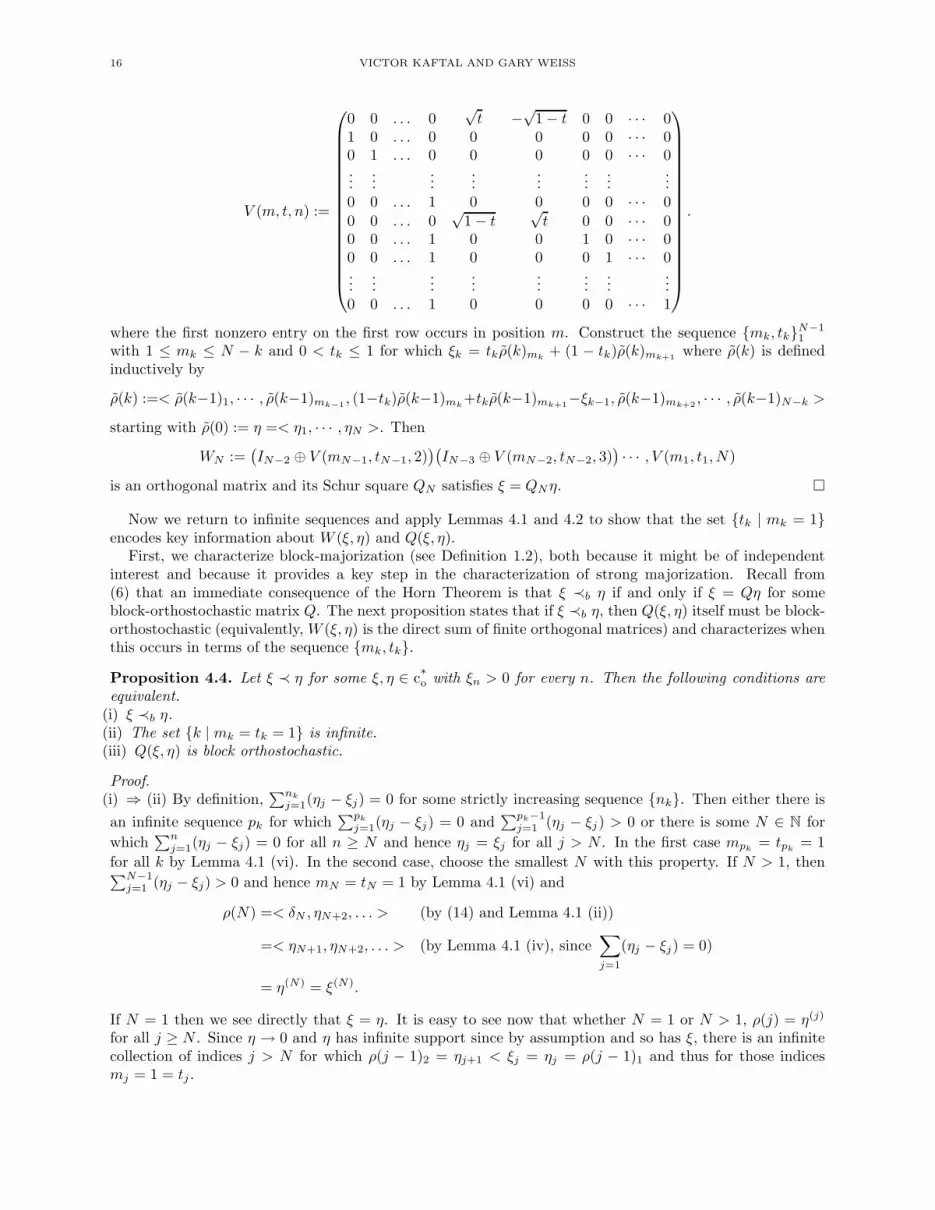
16 VICTOR KAFTAL AND GARY WEISS
V (m, t, n) :=
0 0 . . . 0√
t −√
1 − t 0 0 · · · 01 0 . . . 0 0 0 0 0 · · · 00 1 . . . 0 0 0 0 0 · · · 0...
......
......
......
...0 0 . . . 1 0 0 0 0 · · · 0
0 0 . . . 0√
1 − t√
t 0 0 · · · 00 0 . . . 1 0 0 1 0 · · · 00 0 . . . 1 0 0 0 1 · · · 0...
......
......
......
...0 0 . . . 1 0 0 0 0 · · · 1
.
where the first nonzero entry on the first row occurs in position m. Construct the sequence {mk, tk}N−11
with 1 ≤ mk ≤ N − k and 0 < tk ≤ 1 for which ξk = tkρ(k)mk+ (1 − tk)ρ(k)mk+1
where ρ(k) is definedinductively by
ρ(k) :=< ρ(k−1)1, · · · , ρ(k−1)mk−1, (1−tk)ρ(k−1)mk
+tkρ(k−1)mk+1−ξk−1, ρ(k−1)mk+2
, · · · , ρ(k−1)N−k >
starting with ρ(0) := η =< η1, · · · , ηN >. Then
WN :=(IN−2 ⊕ V (mN−1, tN−1, 2)
)(IN−3 ⊕ V (mN−2, tN−2, 3)
)· · · , V (m1, t1, N)
is an orthogonal matrix and its Schur square QN satisfies ξ = QNη. �
Now we return to infinite sequences and apply Lemmas 4.1 and 4.2 to show that the set {tk | mk = 1}encodes key information about W (ξ, η) and Q(ξ, η).
First, we characterize block-majorization (see Definition 1.2), both because it might be of independentinterest and because it provides a key step in the characterization of strong majorization. Recall from(6) that an immediate consequence of the Horn Theorem is that ξ ≺b η if and only if ξ = Qη for someblock-orthostochastic matrix Q. The next proposition states that if ξ ≺b η, then Q(ξ, η) itself must be block-orthostochastic (equivalently, W (ξ, η) is the direct sum of finite orthogonal matrices) and characterizes whenthis occurs in terms of the sequence {mk, tk}.
Proposition 4.4. Let ξ ≺ η for some ξ, η ∈ c*o with ξn > 0 for every n. Then the following conditions are
equivalent.(i) ξ ≺b η.(ii) The set {k | mk = tk = 1} is infinite.(iii) Q(ξ, η) is block orthostochastic.
Proof.(i) ⇒ (ii) By definition,
∑nk
j=1(ηj − ξj) = 0 for some strictly increasing sequence {nk}. Then either there is
an infinite sequence pk for which∑pk
j=1(ηj − ξj) = 0 and∑pk−1
j=1 (ηj − ξj) > 0 or there is some N ∈ N for
which∑n
j=1(ηj − ξj) = 0 for all n ≥ N and hence ηj = ξj for all j > N . In the first case mpk= tpk
= 1
for all k by Lemma 4.1 (vi). In the second case, choose the smallest N with this property. If N > 1, then∑N−1
j=1 (ηj − ξj) > 0 and hence mN = tN = 1 by Lemma 4.1 (vi) and
ρ(N) =< δN , ηN+2, . . . > (by (14) and Lemma 4.1 (ii))
=< ηN+1, ηN+2, . . . > (by Lemma 4.1 (iv), since∑
j=1
(ηj − ξj) = 0)
= η(N) = ξ(N).
If N = 1 then we see directly that ξ = η. It is easy to see now that whether N = 1 or N > 1, ρ(j) = η(j)
for all j ≥ N . Since η → 0 and η has infinite support since by assumption and so has ξ, there is an infinitecollection of indices j > N for which ρ(j − 1)2 = ηj+1 < ξj = ηj = ρ(j − 1)1 and thus for those indicesmj = 1 = tj .

INFINITE DIMENSIONAL SCHUR-HORN THEOREM 17
(ii) ⇒ (iii) By Lemma 4.2(ii), W (ξ, η) commutes with every Pk for which mk = tk = 1. Thus W (ξ, η) isblock diagonal with each (finite) block an orthogonal matrix and hence its Schur-square Q(ξ, η) is blockorthostochastic.
(iii) ⇒ (i) Obvious (see (6)). �
Next, we proceed to characterize strong majorization ξ 4 η. To do so, we will first need to further analyzethe property obtained in Proposition 3.6 (i) that for every n the orthogonal matrix W (n) has in each columnat most one non-zero entry below row n. For a given j, define
q(n, j) = γ(n, j) = 0 if all the entries of W(n)ij for i > n are zero(18)
W(n)n+q(n,j),j = γ(n, j) is the unique nonzero entry.
Reformulating (18) in vector form,
(19)
W(n)n+1,j
W(n)n+2,j
. . .
=
{
0 if q(n, j) = 0
γ(n, j)eq(n,j) if q(n, j) 6= 0.
and thus we obtain the recurrence relation
W(n+1)n+1,j
W(n+1)n+2,j
. . .
=
(V (mn+1, tn+1) ⊕ I∞
)
W(n)n+1,j
W(n)n+2,j
. . .
=
{
0 if q(n, j) = 0
γ(n, j)(V (mn+1, tn+1) ⊕ I∞
)eq(n,j) if q(n, j) 6= 0
.
We leave to the reader to verify the following lemma.
Lemma 4.5. Given a sequence {mk, tk} where mk ∈ N and 0 < tk ≤ 1, and the co-isometryW := W ({mk, tk}), for every n, j, let q(n, j) and γ(n, j) be the sequences defined by (18)
(i)
q(1, j) =
j for j < m1
j for j = m1, t1 6= 1
0 for j = m1, t1 = 1
j − 1 for j > m1
, γ(1, j) =
1 for j < m1√1 − t1 for j = m1√t1 for j = m1 + 1
1 for j > m1 + 1
,
and
q(n + 1, j) =
q(n, j) for q(n, j) < mn+1
q(n, j) for q(n, j) = mn+1, tn+1 6= 1
0 for q(n, j) = mn+1, tn+1 = 1
q(n, j) − 1 for q(n, j) > mn+1
,
γ(n + 1, j) =
γ(n, j) for q(n, j) < mn+1√1 − tn+1γ(n, j) for q(n, j) = mn+1√tn+1γ(n, j) for q(n, j) = mn+1 + 1
γ(n, j) for q(n, j) > mn+1 + 1
.
(ii) 0 ≤ q(n + 1, j) ≤ q(n, j) ≤ j and 0 ≤ γ(n + 1, j) ≤ γ(n, j) ≤ 1 for every n and j.(iii) ||P⊥
n W (n)ej|| = γ(n, j) for every n and j.(iv) For all n > 1 and all j,
Wnj = W(n))nj =
{
0 if q(n − 1, j) = 0
γ(n − 1, j)(V (mn, tn) ⊕ I∞)
1,q(n−1,j)if q(n − 1, j) 6= 0
.
In particular, all the entries of W are either 0, 1, or products of a finite number of the factors√
tk,√
1 − tkand −√
1 − tk, but not more than one for each k.

18 VICTOR KAFTAL AND GARY WEISS
The case j = 1 is of special use.
Lemma 4.6. Given a sequence {mk, tk} where mk ∈ N and 0 < tk ≤ 1, and the co-isometryW := W ({mk, tk}), let gn := γ(n, 1)2 and set g∞ := lim gn. Then
(i) g∞ =
{
1 mk > 1 for all k∏{(1 − tk) | mk = 1} otherwise
(ii) Wn1 =
{√tngn−1 if mn = 1
0 if mn > 1
(iii) ||We1||2 = 1 − g∞.
Proof.(i) It is straightforward to solve the recurrence relation in Lemma 4.5 (i) for j = 1 and obtain
q(n, 1) =
{
0 if mk = 1, tk = 1 for some 1 ≤ k ≤ n
1 otherwise,
γ(n, 1) =
{
1 if mk > 1 for all 1 ≤ k ≤ n∏{√1 − tk | mk = 1, 1 ≤ k ≤ n} otherwise.
Now (i) follows immediately.(ii) By the proof of (i), q(n, 1) ∈ {0, 1} for all n and thus
Wn1 =
{
0 q(n − 1, 1) = 0
γ(n − 1, 1)(V (mn, tn) ⊕ I∞)1,1 q(n − 1, 1) = 1
(by Lemma 4.5(iv))
=
{
0 q(n − 1, 1) = 0√
gn−1
(V (mn, tn))1,1 q(n − 1, 1) = 1
=√
gn−1
{√tn mn = 1
0 mn > 1(q(n − 1, 1) = 0 ⇔ gn−1 = 0).
(iii) Assume first that the set {k | mk = 1} is non-empty and order it into a strictly increasing, possibly finite,sequence {kn}1≤n≤N≤∞. If N = ∞, then g∞ = limn gkn
. If N < ∞, then gk = gkNfor every k ≥ kN , and
hence g∞ = gkN. Furthermore, for every 1 ≤ n ≤ N , gkn−1 = gkn−1 , where we set n0 = 0 and go = 1. Thus
tkngkn−1 = gkn−1 − gkn
. But then, from (ii) we have
||We1||2 =
N∑
n=1
tkngkn−1 =
N∑
n=1
(gkn−1 − gkn) = gk0 − lim gk = 1 − g∞.
Finally, if the set {k | mk = 1} is empty, then gk = 1 for all k by (i) and hence g∞ = 1. By (ii), Wn1 = 0 forall n and hence ||We1||2 = 0, also satisfying (iii).
�
Theorem 4.7. Let ξ ≺ η for some ξ, η ∈ c*o with ξn > 0 for every n. Then the following conditions are
equivalent.(i) ξ 4 η.(ii)
∑{tk | mk = 1} = ∞.(iii) Q(ξ, η) is orthostochastic.
Proof. Notice that by Lemma 2.4 (see also Remark 2.6 (ii)), Q(ξ, η) is orthostochastic if and only if W (ξ, η)is unitary, in fact, orthogonal, since it has real entries.
(iii) ⇒ (ii) In the case that there are infinitely many indices k for which mk = 1 and tk = 1, then∑{tk | mk = 1} = ∞ holds trivially, thus assume that there is an integer N for which there are no
INFINITE DIMENSIONAL SCHUR-HORN THEOREM 19
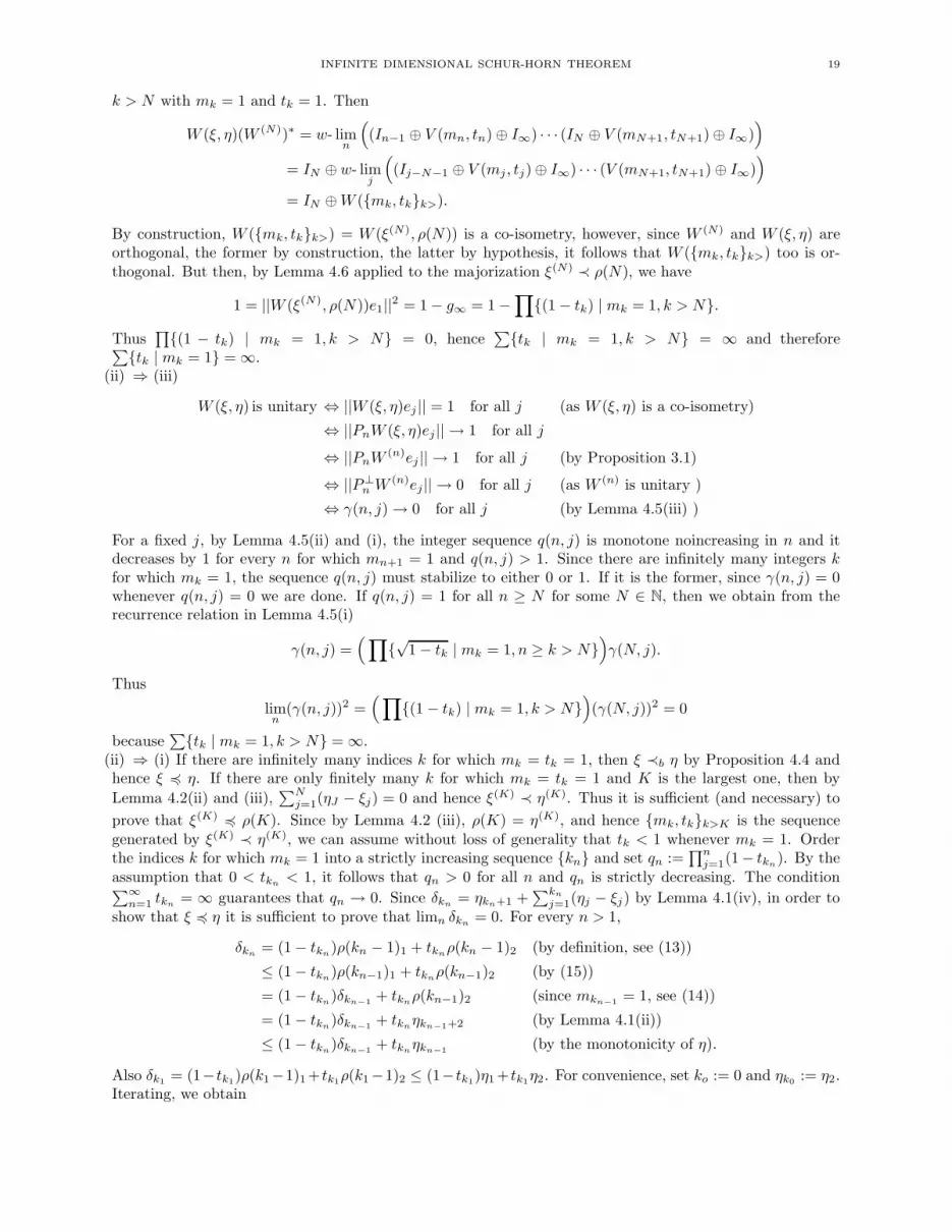
k > N with mk = 1 and tk = 1. Then
W (ξ, η)(W (N))∗ = w- limn
(
(In−1 ⊕ V (mn, tn) ⊕ I∞) · · · (IN ⊕ V (mN+1, tN+1) ⊕ I∞))
= IN ⊕ w- limj
(
(Ij−N−1 ⊕ V (mj , tj) ⊕ I∞) · · · (V (mN+1, tN+1) ⊕ I∞))
= IN ⊕ W ({mk, tk}k>).
By construction, W ({mk, tk}k>) = W (ξ(N), ρ(N)) is a co-isometry, however, since W (N) and W (ξ, η) areorthogonal, the former by construction, the latter by hypothesis, it follows that W ({mk, tk}k>) too is or-thogonal. But then, by Lemma 4.6 applied to the majorization ξ(N) ≺ ρ(N), we have
1 = ||W (ξ(N), ρ(N))e1||2 = 1 − g∞ = 1 −∏
{(1 − tk) | mk = 1, k > N}.
Thus∏{(1 − tk) | mk = 1, k > N} = 0, hence
∑{tk | mk = 1, k > N} = ∞ and therefore∑{tk | mk = 1} = ∞.
(ii) ⇒ (iii)
W (ξ, η) is unitary ⇔ ||W (ξ, η)ej || = 1 for all j (as W (ξ, η) is a co-isometry)
⇔ ||PnW (ξ, η)ej || → 1 for all j
⇔ ||PnW (n)ej || → 1 for all j (by Proposition 3.1)
⇔ ||P⊥n W (n)ej || → 0 for all j (as W (n) is unitary )
⇔ γ(n, j) → 0 for all j (by Lemma 4.5(iii) )
For a fixed j, by Lemma 4.5(ii) and (i), the integer sequence q(n, j) is monotone noincreasing in n and itdecreases by 1 for every n for which mn+1 = 1 and q(n, j) > 1. Since there are infinitely many integers kfor which mk = 1, the sequence q(n, j) must stabilize to either 0 or 1. If it is the former, since γ(n, j) = 0whenever q(n, j) = 0 we are done. If q(n, j) = 1 for all n ≥ N for some N ∈ N, then we obtain from therecurrence relation in Lemma 4.5(i)
γ(n, j) =(∏
{√
1 − tk | mk = 1, n ≥ k > N})
γ(N, j).
Thus
limn
(γ(n, j))2 =(∏
{(1 − tk) | mk = 1, k > N})
(γ(N, j))2 = 0
because∑{tk | mk = 1, k > N} = ∞.
(ii) ⇒ (i) If there are infinitely many indices k for which mk = tk = 1, then ξ ≺b η by Proposition 4.4 andhence ξ 4 η. If there are only finitely many k for which mk = tk = 1 and K is the largest one, then by
Lemma 4.2(ii) and (iii),∑N
j=1(ηJ − ξj) = 0 and hence ξ(K) ≺ η(K). Thus it is sufficient (and necessary) to
prove that ξ(K) 4 ρ(K). Since by Lemma 4.2 (iii), ρ(K) = η(K), and hence {mk, tk}k>K is the sequencegenerated by ξ(K) ≺ η(K), we can assume without loss of generality that tk < 1 whenever mk = 1. Orderthe indices k for which mk = 1 into a strictly increasing sequence {kn} and set qn :=
∏nj=1(1− tkn
). By theassumption that 0 < tkn
< 1, it follows that qn > 0 for all n and qn is strictly decreasing. The condition∑∞
n=1 tkn= ∞ guarantees that qn → 0. Since δkn
= ηkn+1 +∑kn
j=1(ηj − ξj) by Lemma 4.1(iv), in order toshow that ξ 4 η it is sufficient to prove that limn δkn
= 0. For every n > 1,
δkn= (1 − tkn
)ρ(kn − 1)1 + tknρ(kn − 1)2 (by definition, see (13))
≤ (1 − tkn)ρ(kn−1)1 + tkn
ρ(kn−1)2 (by (15))
= (1 − tkn)δkn−1 + tkn
ρ(kn−1)2 (since mkn−1 = 1, see (14))
= (1 − tkn)δkn−1 + tkn
ηkn−1+2 (by Lemma 4.1(ii))
≤ (1 − tkn)δkn−1 + tkn
ηkn−1 (by the monotonicity of η).
Also δk1 = (1− tk1)ρ(k1−1)1+ tk1ρ(k1−1)2 ≤ (1− tk1)η1 + tk1η2. For convenience, set ko := 0 and ηk0 := η2.Iterating, we obtain

20 VICTOR KAFTAL AND GARY WEISS
δkn≤(
n∏
j=2
(1 − tkj))(
(1 − tk1)η1 + tk1η2
)+
n∑
j=3
(
tkj−1
n∏
i=j
(1 − tki)ηkj−2
)
+ tknηkn−1
=(
n∏
i=1
(1 − tki))η1 +
n∑
j=2
(
tkj−1
n∏
i=j
(1 − tki)ηkj−2
)
+ tknηkn−1
=(
n∏
i=1
(1 − tki))η1 +
n∑
j=2
(( n∏
i=j
(1 − tki) −
n∏
i=j−1
(1 − tki))
ηkj−2
)
+ (1 − (1 − tkn))ηkn−1
= qnη1 +
n∑
j=2
( qn
qj−1− qn
qj−2
)
ηkj−2 +(1 − qn
qn−1
)ηkn−1
= qn
(
η1 +
n∑
j=2
( 1
qj−1− 1
qj−2
)
ηkj−2 −1
qn−1ηkn−1
)
+ ηkn−1
= qn(η1 − η2) + qn
n∑
j=2
1
qj−1(ηkj−2 − ηkj−1 ) + ηkn−1 ,
where the last equality is obtained by “summation by parts”. We know that qn → 0 and clearly, ηkn−1 → 0.
We claim that also qn
∑nj=2
1qj−1
(ηkj−2 − ηkj−1 ) → 0. Indeed, for every ǫ > 0, choose m for which ηkm< ǫ
and choose N ≥ m + 2 so that for all n ≥ N
qn
m+1∑
j=2
1
qj−1(ηkj−2 − ηkj−1 ) < ǫ.
Then by the monotonicity of q and η
qn
n∑
j=2
1
qj−1(ηkj−2 − ηkj−1 ) < ǫ + qn
n∑
j=m+2
1
qj−1(ηkj−2 − ηkj−1 )
≤ ǫ +
n∑
j=m+2
(ηkj−2 − ηkj−1) < ǫ + ηkm< 2ǫ.
This proves that limn δkn= 0 and hence that ξ 4 η.
We split the proof of the implication (i) ⇒ (ii) or (iii) in two cases.If η has infinite support, then (i) ⇒ (iii). Immediate by Remark 3.10.If η has finite support, then (i) ⇒ (ii). Let ηN > 0 and ηN+1 = 0. First notice that if mh = 1 for someh ≥ N−1, then ρ(h)2 = ηh+2 = 0 by Lemma 4.1 (ii). For every k ≥ h, ρ(k)2 ≤ ρ(h)2, hence ρ(k)2 = 0 and bythe definition of mk we have mk = 1. Thus the sequence {mk} either eventually stabilizes at 1 or is boundedaway from 1 from N −1 on. We claim that the latter case is impossible. Reasoning by contradiction, assumethat mk ≥ 2 for all k ≥ N − 1. Then for every k ≥ N − 1 and every n ≥ mk we have
ξN ≤ ρ(N − 1)1 (since ξ(N−1) ≺ ρ(N − 1) by (15))
= ρ(k)1 (by (14)
≤n∑
j=1
ρ(k)j
=
n+k∑
j=1
ηj −k∑
j=1
ξj (by Lemma 4.1(iii))
=
∞∑
j=k+1
ξj → 0 (since
N∑
j=1
ηj =
∞∑
j=1
ξj)
which contradicts the assumption that ξ has infinite support and hence ξN > 0. Therefore there is a K ≥ Nsuch that mk = 1 for all k ≥ K. But then, if k > K, ρ(k − 1) =< δk−1, 0, . . . > and hence ξk = tkδk−1,
INFINITE DIMENSIONAL SCHUR-HORN THEOREM 21
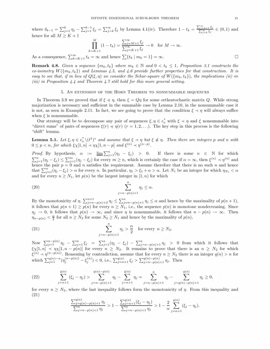
where δk−1 =∑k
j=1 ηj −∑k−1
j=1 ξj =∑∞
j=k ξj by Lemma 4.1(iv). Therefore 1 − tk =P
∞
j=k+1 ξjP
∞
j=k ξj∈ (0, 1) and
hence for all M ≥ K + 1M∏
k=K+1
(1 − tk) =
∑∞j=M+1 ξj
∑∞j=K+1 ξj
→ 0 for M → ∞.
As a consequence,∑∞
k=K+1 tk = ∞ and hence∑{tk | mk = 1} = ∞. �
Remark 4.8. Given a sequence {mk, tk} where mk ∈ N and 0 < tk ≤ 1, Proposition 3.1 constructs theco-isometry W ({mk, tk}) and Lemmas 4.5, and 4.6 provide further properties for that construction. It iseasy to see that, if in lieu of Q(ξ, η) we consider the Schur-square of W ({mk, tk}), the implications (ii) ⇔(iii) in Proposition 4.4 and Theorem 4.7 still hold for this more general setting.
5. An extension of the Horn Theorem to nonsummable sequences
In Theorem 3.9 we proved that if ξ 4 η, then ξ = Qη for some orthostochastic matrix Q. While strongmajorization is necessary and sufficient in the summable case by Lemma 2.10, in the nonsummable case itis not, as seen in Example 2.11. In fact, we are going to prove that the condition ξ ≺ η will always sufficewhen ξ is nonsummable.
Our strategy will be to decompose any pair of sequences ξ, η ∈ c*o with ξ ≺ η and ξ nonsummable into
“direct sums” of pairs of sequences ξ(r) 4 η(r) (r = 1, 2, . . .). The key step in this process is the following“shift” lemma.
Lemma 5.1. Let ξ, η ∈ c*o \(ℓ1)∗ and assume that ξ ≺ η but ξ 64 η. Then there are integers p and n with
0 ≤ p < n, for which ξχ[1, n] ≺ ηχ[1, n − p] and ξ(n) ≺ η(n−p).
Proof. By hypothesis, α := lim∑n
j=1(ηj − ξj) > 0. If there is some n ∈ N for which∑n
j=1(ηj − ξj) ≤∑m
j=1(ηj − ξj) for every m ≥ n, which is certainly the case if α = ∞, then ξ(n) ≺ η(n) andhence the pair p = 0 and n satisfies the requirement. Assume therefore that there is no such n and hencethat
∑nj=1(ηj − ξj) > α for every n. In particular, η1 > ξ1 + α > α. Let N1 be an integer for which ηN1 < α
and for every n ≥ N1, let p(n) be the largest integer in [1, n) for which
(20)n∑
j=n−p(n)+1
ηj ≤ α.
By the monotonicity of η,∑n+1
j=n−p(n)+2 ηj ≤∑nj=n−p(n)+1 ηj ≤ α and hence by the maximality of p(n + 1),
it follows that p(n + 1) ≥ p(n) for every n ≥ N1, i.e., the sequence p(n) is monotone nondecreasing. Sinceηj → 0, it follows that p(n) → ∞, and since η is nonsummable, it follows that n − p(n) → ∞. Thenηn−p(n) < α
2 for all n ≥ N2 for some N2 ≥ N1 and hence by the maximality of p(n),
(21)
n∑
j=n−p(n)+1
ηj >α
2for every n ≥ N2.
Now∑n−p(n)
j=1 ηj − ∑nj=1 ξj =
∑nj=1(ηj − ξj) − ∑n
j=n−p(n)+1 ηj > 0 from which it follows that
ξχ[1, n] ≺ ηχ[1, n − p(n)] for every n ≥ N2. It remains to prove that there is an n ≥ N2 for whichξ(n) ≺ η(n−p(n)). Reasoning by contradiction, assume that for every n ≥ N2 there is an integer q(n) > n for
which∑q(n)−n
j=1 (η(n−p(n))j − ξ
(n)j ) < 0, i.e.,
∑q(n)j=n+1 ξj >
∑q(n)−p(n)j=n−p(n)+1 ηj . Then
(22)
q(n)∑
j=n+1
(ξj − ηj) >
q(n)−p(n)∑
j=n−p(n)+1
ηj −q(n)∑
j=n+1
ηj =n∑
j=n−p(n)+1
ηj −q(n)∑
j=q(n)−p(n)+1
ηj ≥ 0,
for every n ≥ N2, where the last inequality follows form the monotonicity of η. From this inequality and(21)
∑q(n)j=q(n)−p(n)+1 ηj∑n
j=n−p(n)+1 ηj> 1 −
∑q(n)j=n+1(ξj − ηj)∑n
j=n−p(n)+1 ηj> 1 − 2
α
q(n)∑
j=n+1
(ξj − ηj).

22 VICTOR KAFTAL AND GARY WEISS
Set m1 = N2 and mk+1 := q(mk). The sequence mk is strictly increasing and for every k ≥ 1,∑mk+1
j=mk+1−p(mk)+1 ηj∑mk
j=mk−p(mk)+1 ηj> 1 − 2
α
mk+1∑
j=mk+1
(ξj − ηj).
Given that η is nonincreasing and that p(mk) is nondecreasing, the average of η over the integer interval{mk+1 − p(mk+1) ≤ j ≤ mk+1} must be larger or equal than its average over the integer interval{mk+1 − p(mk) ≤ j ≤ mk+1} and hence
(23)
1p(mk+1)
∑mk+1
j=mk+1−p(mk+1)+1 ηj
1p(mk)
∑mk
j=mk−p(mk)+1 ηj
≥1
p(mk)
∑mk+1
j=mk+1−p(mk)+1 ηj
1p(mk)
∑mk
j=mk−p(mk)+1 ηj
> 1 − 2
α
mk+1∑
j=mk+1
(ξj − ηj).
Now by (22),∑mk+1
j=mk+1(ξj − ηj) > 0 for every k ≥ 1 and by assumption,∑mk
j=1(ηj − ξj) > α > 0. Thus forevery h > 1,
mh∑
j=1
(ηj − ξj) =
m1∑
j=1
(ηj − ξj) −mh∑
j=m1+1
(ξj − ηj) =
m1∑
j=1
(ηj − ξj) −h−1∑
k=1
mk+1∑
j=mk+1
(ξj − ηj) > 0,
whence∑∞
k=1
∑mk+1
j=mk+1(ξj −ηj) < ∞. Choose ko ∈ N for which∑∞
k=ko
∑mk+1
j=mk+1(ξj −ηj) < α2 . In particular,
for all k ≥ ko we have 0 < 2α
∑mk+1
j=mk+1(ξj − ηj) < 1 and hence from equation (23) we have for every K ≥ ko
0 <
K∏
k=ko
(
1 − 2
α
mk+1∑
j=mk+1
(ξj − ηj)
)
<
1p(mK+1)
∑mK+1
j=mK+1−p(mK+1)+1 ηj
1p(mko )
∑mko
j=mko−p(mko )+1 ηj
≤ 2p(mko
)
p(mK+1),
where the last inequality follows from the inequalites (20) and (21). Now, on the one hand, p(mk) → ∞and hence 2
p(mko )p(mK+1) → 0 for K → ∞. On the other hand, the sequence 2
α
∑mk+1
j=mk+1(ξj − ηj) ∈ (0, 1) and is
summable, hence∏∞
k=ko
(
1 − 2α
∑mk+1
j=mk+1(ξj − ηj)
)
> 0, a contradiction.
�
Lemma 5.2. Let ξ, η ∈ c*o \(ℓ1)∗ and assume that ξ ≺ η but ξ 64 η. Then there there are two partitions of N
into sequences, N = {n(1)j } ∪ {n(2)
j } and N = {m(1)j } ∪ {m(2)
j } with n(1)1 = m
(1)1 = 1 for which, if ξ′ := {ξ
n(1)j
},η′ := {η
m(1)j
}, ξ′′ := {ξn
(2)j
}, and η′′ := {ηm
(2)j
} are the corresponding subsequences of ξ and η, then ξ′ 4 η′,
ξ′′ ≺ η′′, ξ′′ 64 η′′, and ξ′ ∈ (ℓ1)∗.
Proof. By Lemma 5.1, ξχ[1, N ] ≺ ηχ[1, N − p] and ξ(N) ≺ η(N−p) for some pair of integers p and N with0 ≤ p < N . Let
α := lim( k∑
j=1
(ηj − ξj))
, β :=
N−p∑
j=1
ηj −N∑
j=1
ξj , and γ := lim( k∑
j=1
(η(N−p)j − ξ
(N)j )
)
.
By hypothesis, α > 0 and β ≥ 0, γ ≥ 0. Since for k > N − p
k∑
j=1
(ηj − ξj) = β +
k−N+p∑
j=1
(η(N−p)j − ξ
(N)j ) +
k+p∑
j=k+1
ξj
and∑k+p
j=k+1 ξj → 0 for k → ∞, it follows that 0 < α = β + γ, so β and γ cannot both vanish.
Assume first that β > 0. The strategy for the construction of the sequences ξ′, ξ′′, η′, and η′′ is to firstmove a finite number of entries from the infinite sequence ξ(N) to the finite sequence ξχ[1, N ], i.e., deletethem from the first sequence and insert them after the last nonzero term of the second one, and do so whilewhile controlling the sum and preserving the majorization by ηχ[1, N − p] of the new finite sequence. Thiswill automatically preserve majorization of the new infinite sequence by η(N−p). At the next step, movea single entry from the sequence η(N−p) to the sequence ηχ[1, N − p], so to preserve majorization of thetwo infinite sequences and still control the sums, while majorization of the two finite ones is automaticallypreserved. And then iterate the process.

INFINITE DIMENSIONAL SCHUR-HORN THEOREM 23
Now we make this strategy precise. We construct three strictly increasing sequences of integers kj , hi andqi with N < kqi
< hi ≤ hi + p < kqi+1 < kqi+2 < · · · < kqi+1 so that
β +
i−1∑
j=1
ηhj− 1
i<
qi∑
j=1
ξkj< β +
i−1∑
j=1
ηhj,(24)
δi :=
qi∑
j=1
ξkj−
kqi+qi∑
j=kqi+1
ξj > δi−1,(25)
ηhi< min{ 1
2i, δi −
i−1∑
j=1
ηhj},(26)
where for i = 1 we take 0 in place of∑i−1
j=1 ηhjand of δi−1.
To start the construction, use the fact that ξj → 0 and is nonsummable to choose N < k1 < · · · < kq1−1
for which β − 1 <∑q1−1
j=1 ξkj< β. Since ξ has infinite support, it has an infinite subsequence for which
ξpn> ξpn+1. Choose kq1 ∈ {pn} large enough so that
∑q1
j=1 ξkj< β. By the monotonicity of ξ, it follows
that δ1 :=∑q1
i=1 ξki−∑kq1+q1
j=kq1+1 ξj > 0 and conditions (24) and (25) are thus satisfied for i = 1. To satisfy
also (26) it is enough to choose h1 > kq1 so that ηh1 < min{ 12 , δ1}, which is always possible since ηj → 0
and δ1 > 0. Assume now the construction of the three integer sequences up to some i − 1 and choosehi−1 + p < kqi−1+1 < kqi−1+2 < · · · < kqi−1 for which
β +i−1∑
j=1
ηhj−
qi−1∑
j=1
ξkj− 1
i<
qi−1∑
j=qi−1+1
ξkj< β +
i−1∑
j=1
ηhj−
qi−1∑
j=1
ξkj.
Choose kqi∈ {pn}, kqi
> kqi−1 large enough so that∑qi
j=qi−1+1 ξkj< β +
∑i−1j=1 ηhj
−∑qi−1
j=1 ξkj, i.e., so to
satisfy (24). Now
δi − δi−1 =
qi∑
j=qi−1+1
ξkj−
kqi+qi∑
j=kqi+1
ξj +
kqi−1+qi−1∑
j=kqi−1+1
ξj
=
qi∑
j=qi−1+1
ξkj−
kqi+qi∑
j=kqi+qi−1+1
ξj +
kqi−1+qi−1∑
j=kqi−1+1
ξj −kqi
+qi−1∑
j=kqi+1
ξj
≥qi∑
j=qi−1+1
ξkj−
kqi+qi∑
j=kqi+qi−1+1
ξj (by the monotonicity of ξ)
> 0. (because ξkqi> ξkqi
+1)
Thus (25) is satisfied. By the induction assumption that ηhn< min{ 1
2n , δn−∑n−1
j=1 ηhj} for all 1 ≤ n ≤ i−1,
we see that δi > δi−1 >∑i−i
j=1 ηhjand since ηn → 0 we can choose hi > kqi
so to satisfy also (26).Now define
(27) n(1) :=< 1, . . . , N, k1, k2, . . . > and m(1) :=< 1, . . . , N − p, h1, h2, . . . >
and n(2), m(2) are the complementary sequences of n(1), m(1) respectively. Explicitly,
ξ′ : = < ξ1, . . . , ξN , ξk1 , ξk2 , . . . > and η′ : = < η1, . . . , ηN−p, ηh1 , ηh2 , . . . >(28)
ξ′′ : = < ξN+1, ξN+2, . . . , ξk1−1, ξk1+1, . . . > and η′′ : = < ηN−p+1, . . . , ηh1−1, ηh1+1, . . . > .
First we verify that ξ′ 4 η′.If m ≤ N − p, then
∑mj=1(η
′j − ξ′j) =
∑mj=1(ηj − ξj) ≥ 0.
If N − p < m ≤ N , then∑m
j=1(η′j − ξ′j) ≥
∑N−pj=1 ηj −
∑Nj=1 ξj = β > 0.
Finally, if m > N , let qi−1 < m − N ≤ qi, where we set qo = 0 for convenience. Then m > N + qi−1 ≥

24 VICTOR KAFTAL AND GARY WEISS
N + i − 1 ≥ N − p + i − 1 and hence
m∑
j=1
η′j ≥
N−p+i−1∑
j=1
η′j =
N−p∑
j=1
ηj +i−1∑
j=1
ηhj
≥N−p∑
j=1
ηj − β +
qi∑
j=1
ξkj(by (26))
=N∑
j=1
ξj +
qi∑
j=1
ξkj≥
N∑
j=1
ξj +m−∑
j=1
ξkj=
m∑
j=1
ξ′j .
Thus ξ′ ≺ η′. For every i > 1,
N−p+i−1∑
j=1
η′j =
N−p∑
j=1
ηj +
i−1∑
j=1
ηhj=
N∑
j=1
ξj + β +
i−1∑
j=1
ηhj(by the definition of β)
≤N∑
j=1
ξj +
qi∑
j=1
ξkj+
1
i(by (26))
=
N+qi∑
j=1
ξ′j +1
i<
∞∑
j=1
ξ′j +1
i.
Therefore∑∞
j=1 η′j ≤∑∞
j=1 ξ′j and since ξ′ ≺ η′ and by (26), η′ ∈ (ℓ1)∗ and hence ξ′ ∈ (ℓ1)∗, equality follows,
i.e., ξ′ 4 η′.Next, we verify that ξ′′ ≺ η′′. We start with the following two inequalities.
If hi + p ≤ N + m < hi+1 + p, then
(29)
m∑
j=1
η′′j =
m+i∑
j=1
η(N−p)j −
i∑
j=1
ηhj≥
m∑
j=1
η(N−p)j −
i∑
j=1
ηhj
If kqi≤ N + m < kqi+1 and N + m ≥ h1 + p, then
m∑
j=1
ξ′′j =
m+qi∑
j=1
ξ(N)j −
qi∑
j=1
ξkj=
m∑
j=1
ξ(N)j +
N+m+qi∑
j=N+m+1
ξj −qi∑
j=1
ξkj(30)
≤m∑
j=1
ξ(N)j +
kqi+qi∑
j=kqi+1
ξj −qi∑
j=1
ξkj=
m∑
j=1
ξ(N)j − δi,
where the inequality follows from the monotonicity of ξ.Since N < h1 + p < kq2 < . . . kqi
< hi ≤ hi + p < kqi+1 < . . . , to prove that∑m
j=1(η′′j − ξ′′j ) ≥ 0, we need to
consider three cases: N + m < h1 + p, hi + p ≤ N + m < kqi+1 for some i ≥ 1, and kqi≤ N + m < hi + p
for some i ≥ 2.In the first case, since ξ(N) ≺ η(N−p),
m∑
j=1
(η′′j − ξ′′j ) =
m∑
j=1
(η(N−p)j − ξ′′j ) ≥
m∑
j=1
(η(N−p)j − ξ
(N)j ) ≥ 0.
In the second case hi + p ≤ N + m < hi+1 + p and kqi≤ N + m < kqi+1 while N + m ≥ h1 + p, hence
combining (29) and (30) yields
m∑
j=1
(η′′j − ξ′′j ) ≥
m∑
j=1
(η(N−p)j − ξ′′j ) + δi −
i∑
j=1
ηhj> 0
where the last inequality follows from ξ(N) ≺ η(N−p) and (26).In the third case hi−1 + p ≤ N + m < hi + p and kqi
≤ N + m < kqi+1 while N + m ≥ kq2 > h1 + p, hence
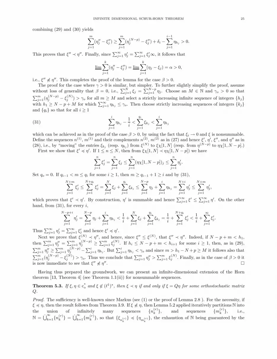
INFINITE DIMENSIONAL SCHUR-HORN THEOREM 25
combining (29) and (30) yields
m∑
j=1
(η′′j − ξ′′j ) ≥
m∑
j=1
(η(N−p)j − ξ′′j ) + δi −
i−1∑
j=1
ηhj> 0.
This proves that ξ′′ ≺ η′′. Finally, since∑∞
j=1 η′j =
∑∞j=1 ξ′j∞, it follows that
lim
k∑
j=1
(η′′j − ξ′′j ) = lim
k∑
j=1
(ηj − ξj) = α > 0,
i.e., ξ′′ 64 η′′. This completes the proof of the lemma for the case β > 0.The proof for the case where γ > 0 is similar, but simpler. To further slightly simplify the proof, assume
without loss of generality that β = 0, i.e.,∑N
j=1 ξj =∑N−p
j=1 ηj . Choose an M ∈ N and γo > 0 so that∑m
j=1(η(N−p)j − ξ
(N)j ) > γo for all m ≥ M and select a strictly increasing infinite sequence of integers {hj}
with h1 ≥ N − p + M for which∑∞
j=1 ηhj≤ γo. Then choose strictly increasing sequences of integers {kj}
and {qi} so that for all i ≥ 1
(31)
i∑
j=1
ηhj− 1
i<
qi∑
j=1
ξkj<
i∑
j=1
ηhj
which can be achieved as in the proof of the case β > 0, by using the fact that ξi → 0 and ξ is nonsummable.Define the sequences n(1), m(1) and their complements n(2), m(2) as in (27) and hence ξ′, η′, ξ′′, and η′′ as in(28), i.e., by “moving” the entries ξkj
(resp. ηkj) from ξ(N) to ξχ[1, N ] (resp. from η(N−p) to ηχ[1, N − p].)
First we show that ξ′ 4 η′. If 1 ≤ n ≤ N , then from ξχ[1, N ] ≺ ηχ[1, N − p]) we have
n∑
j=1
ξ′j =
n∑
j=1
ξj ≤n∑
j=1
(ηχ[1, N − p])j ≤n∑
j=1
η′j .
Set qo = 0. If qi−1 < m ≤ qi for some i ≥ 1, then m ≥ qi−1 + 1 ≥ i and by (31),
N+m∑
j=1
ξ′j ≤N+qi∑
j=1
ξ′j =
N∑
j=1
ξj +
qi∑
j=1
ξkj≤
N−p∑
j=1
ηj +
i∑
j=1
ηhj=
N+i∑
j=1
η′j ≤
N+m∑
j=1
η′j ,
which proves that ξ′ ≺ η′. By construction, η′ is summable and hence∑∞
j=1 ξ′ ≤ ∑∞j=1 η′. On the other
hand, from (31), for every i,
N−p+i∑
j=1
η′j =
N−p∑
j=1
ηj +
i∑
j=1
ηhj<
1
i+
N∑
j=1
ξj +
qi∑
j=1
ξkj=
1
i+
N+qi∑
j=1
ξ′j <1
i+
∞∑
j=1
ξ′j .
Thus∑∞
j=1 η′j =
∑∞j=1 ξ′j and hence ξ′ 4 η′.
Next we prove that ξ(N) ≺ η′′, and hence, since ξ′′ ≤ ξ(N), that ξ′′ ≺ η′′. Indeed, if N − p + m < h1,
then∑m
j=1 η′′j =
∑mj=1 η
(N−p)j ≥ ∑m
j=1 ξ(N)j . If hi ≤ N − p + m < hi+1 for some i ≥ 1, then, as in (29),
∑mj=1 η′′
j ≥∑mj=1 η
(N−p)j −∑i
j=1 ηhj. But
∑ij=1 ηhj
< γo and since m > h1 −N + p ≥ M it follows also that∑m
j=1(η(N−p)j − ξ
(N)j ) > γo. Thus we conclude that
∑mj=1 η′′
j >∑m
j=1 ξ(N)j . Finally, as in the case of β > 0 it
is now immediate to see that ξ′′ 64 η′′. �
Having thus prepared the groundwork, we can present an infinite-dimensional extension of the Horntheorem [13, Theorem 4] (see Theorem 1.1(ii)) for nonsummable sequences.
Theorem 5.3. If ξ, η ∈ c*o and ξ 6∈ (ℓ1)∗, then ξ ≺ η if and only if ξ = Qη for some orthostochastic matrix
Q.
Proof. The sufficiency is well-known since Markus (see (1) or the proof of Lemma 2.8 ). For the necessity, ifξ 4 η, then the result follows from Theorem 3.9. If ξ 64 η, then Lemma 5.2 applied iteratively partitions N into
the union of infinitely many sequences {n(r)k }, and sequences {m(r)
k }, i.e.,
N = ˙⋃∞k=1{n
(r)k } = ˙⋃∞
k=1{m(r)k }, so that {ξ
n(r)k
} 4 {ηm
(r)k
}, the exhaustion of N being guaranteed by the

26 VICTOR KAFTAL AND GARY WEISS
condition in Lemma 5.2 that n(1)1 = m
(1)1 = 1. Then by Theorem 3.9 we can find for each r an orthogonal
matrix W (r) with Schur-square Q(r), for which {ξn
(r)k
} = Q(r){ηm
(r)k
}. “Direct summing” the matrices Q(r)
with respect to the two decompositions of the basis yields the required orthostochastic matrix Q. Explicitly,let Rr, Sr ∈ B(H) be the diagonal projections on the subspaces with bases {e
m(r)k
} and {em
(r)k
} respectively.
Then∑∞
r=1 Rr =∑∞
r=1 Sr = I. We can identify the matrices Q(r) and W (r) with corresponding operators inB(RrH, SrH) and then define Q :
∑∞r=1 SrQ(r)Rr and W :
∑∞r=1 SrW (r)Rr . It is clear that W, Q ∈ B(H),
W is unitary and its matrix is
Wij :=
{
(W (r))hk if i = n(r)h , j = m
(r)k for some r, h, k
0 otherwise.
Similarly,
Qij :=
{
(Q(r))hk if i = n(r)h , j = m
(r)k for some r, h, k
0 otherwise.
Thus the matrix Q is the Schur-square of the matrix W and hence Q is orthostochastic. For every i ∈ N,
i = n(r)h for a unique r and h and
(Qη)i =
∞∑
j=1
Qijηj =
∞∑
k=1
Q(r)hkηm
(r)k
= ξn
(r)h
= ξi
i.e., ξ = Qη. �
Thus combining the above theorem with Theorem 3.9, we have the following infinite dimensional extensionof the Horn Theorem
Remark 5.4. If ξ, η ∈ c*o then ξ = Qη for some orthostochastic matrix Q ⇐⇒
{
ξ ≺ η if ξ 6∈ ℓ1
ξ 4 η if ξ ∈ ℓ1.
6. Diagonals of compact operators
Recall that having fixed an orthonormal basis for the Hilbert space H , we denote by D the masa ofdiagonal operators, by E : B(H) → D the operation of taking the main diagonal, i.e., the normal faithfuland trace preserving conditional expectation from B(H) onto D, and by diag : ℓ∞ → D the isometricisomorphism that maps a sequence η to the diagonal operator having diagonal η.
For the readers’ convenience, let us first collect here some of the equivalent conditions of the majorizationrelations that we have obtained explicitly or that are immediate consequences of results obtained in theprevious sections.
Corollary 6.1. Let ξ, η ∈ c*o .
If ξ 6∈ (ℓ1)∗, then the following conditions are equivalent:NS(i) ξ ≺ ηNS(ii) ξ = Qη for some orthostochastic matrix Q.NS(ii′) diag ξ = E(U diag ηU∗) for some orthogonal matrix U .NS(iiid) ξ = Qη for some doubly stochastic matrix Q.NS(iiis) ξ = Qη for some substochastic matrix Q.NS(iii′is) diag ξ = E(W diag ηW ∗) for some isometry W .NS(iii′cs) diag ξ = E(W diag ηW ∗) for some co-isometry W .NS(iii′cn) diag ξ = E(L diag ηL∗) for some contraction L.If ξ ∈ (ℓ1)∗, then the following conditions are equivalent:
S(i) ξ 4 ηS(ii) ξ = Qη for some orthostochastic matrix Q.S(ii′) diag ξ = E(U diag ηU∗) for some orthogonal matrix U .S(iiid) ξ = Qη for some doubly stochastic matrix Q.S(iiic) ξ = Qη for some column stochastic matrix Q.S(iii′is) diag ξ = E(W diag ηW ∗) for some isometry W .In general the following conditions are equivalent:
INFINITE DIMENSIONAL SCHUR-HORN THEOREM 27
(i) ξ ≺ η.(ii) ξ = DQη for some orthostochastic matrix Q and some D ∈ D with 0 ≤ D ≤ I.(iii) ξ = QDη for some orthostochastic matrix Q and some D ∈ D with 0 ≤ D ≤ I.(ii′) diag ξ = E(DU diag η (DU)∗) = for some orthogonal U and some D ∈ D with 0 ≤ D ≤ I.(iii′) diag ξ = E(UD diag η (UD)∗) for some orthogonal U and some D ∈ D with 0 ≤ D ≤ I.(iv) diag ξ = E(L diag ηL∗) for some contraction L.
Remark 6.2.
(i) In lieu of orthogonal matrices it suffices to take unitary matrices and conversely, we can always ask thatthe isometries, co-isometries, and contractions have real entries.
(ii) The equivalence of (i) and (iv) was proven by Arveson and Kadison in [3, Theorem 4.2]
In the case of finite rank positive operators, the “sequence” formulation S(i)⇔S(ii′) in the above corollaryis obviously equivalent to the operator theory formulation of the classical Schur-Horn Theorem (see Theorem1.1 (iii)).
For infinite rank positive compact operators however, the above corollary leads to a somewhat differentoperator theory reformulation. We find convenient to introduce the notion of partial isometry orbit of anoperator.
For every operator A ∈ B(H), denote by
U(A) : = {UAU∗ | U unitary in B(H)} the unitary orbit of A.
V(A) : = {V AV ∗ | V partial isometry in B(H), V ∗V = RA ∨ RA∗} the partial isometry orbit of A.
Lemma 6.3. U(A) ⊂ V(A) for every A ∈ B(H) and U(A) = V(A) if and only if A has finite rank.
Proof. The inclusion is obvious since if U is unitary, then V := U(RA ∨ RA∗) is a partial isometry withV ∗V = RA ∨ RA∗ and UAU∗ = V AV ∗.
If A has finite rank and V is a partial isometry with V ∗V = RA ∨ RA∗ , then both (V ∗V )⊥ and (V V ∗)⊥
are infinite and hence equivalent projections. Thus V can be extended to a unitary U and V AV ∗ = UAU∗.Thus U(A) = V(A).
If A has infinite rank, then choose a partial isometry V with V ∗V = RA ∨ RA∗ but (V V ∗)⊥ 6∼ (V ∗V )⊥
and let B = V AV ∗. Since V RAV ∗B = V RAV ∗V AV ∗ = B, it follows that V V ∗ ≥ V RAV ∗ ≥ RB. Similarly,V RA∗V ∗B∗ = B∗ and hence V V ∗ ≥ V RA∗V ∗ ≥ RB∗ . Thus V V ∗ ≥ V (RA∨RA∗)V ∗ = V RAV ∗∨V RA∗V ∗ ≥RB∨RB∗ . So far, we have only used the fact that V ∗V ≥ RA∨RA∗ , and since A = V ∗BV , the same argumentshows that V ∗(RB ∨ RB∗)V ≥ RA ∨ RA∗ . But then
RB ∨ RB∗ ≤ V V ∗ = V (RA ∨ RA∗)V ∗ ≤ V V ∗(RB ∨ RB∗)V V ∗ = RB ∨ RB∗
whence V V ∗ = RB ∨RB∗ . But then RB ∨RB∗ is not unitarily equivalent to RA∨RA∗ , hence B 6∈ U(A). �
Denote by s(A) the sequence of s-numbers of A. In particular, if A is a positive compact operator, s(A) isthe eigenvalue list of A in monotone non-increasing order, with repetition according to multiplicity, and withinfinitely many zeros added in case A has finite rank. Notice that the eigenvalue list of A “ignores” the nullspace of A, i.e., s(A) = s(A⊕ 0n) where 0n denotes the zero operator on a space of dimension n ∈ N∪ {∞}.
Since for all A ∈ K(H)+ there is an isometry V for which A = V diag s(A)V ∗ (and V can be chosenunitary when A has finite rank or when RA = I), we see that
(32) V(A) = V(diag s(A)) = {B ∈ K(H)+ | s(B) = s(A)} =⋃
0≤n≤∞U(diag s(A) ⊕ 0n).
In [3] the set V(A) is denoted by Os(A) and it was shown that V(A) = U(A))||.||1
when A is trace-class,[3,Proposition 3.1].
The infinite dimensional extensions of the Horn Theorem obtained in Theorems 3.9 and 5.3 provide acharacterization of “the diagonals” of the partial isometry orbit of a positive compact operator.
Proposition 6.4. Let A ∈ K(H)+. Then
E(V(A)) =
{
{B ∈ D ∩ K(H)+ | s(B) ≺ s(A)} \ L1 if Tr(A) = ∞{B ∈ D ∩ K(H)+ | s(B) 4 s(A)} if Tr(A) < ∞.

28 VICTOR KAFTAL AND GARY WEISS
Proof. By (32), assume without loss of generality that A = diag s(A).To prove that the left hand set is contained in the right hand set, let V be a partial isometry with V ∗V =
Rdiag s(A) and let B = E(V diag s(A)V ∗). Then Tr(B) = Tr(V diag s(A)V ∗) = Tr(diag s(A)) = Tr(A) andwe only need to prove that s(B) ≺ s(A). Let W be the isometry that rearranges the sequence s(B) into thesequence of the diagonal entries of B, i.e., B = W diag s(B)W ∗. Then W commutes with the expectation Eand hence
diag s(B) = W ∗BW = W ∗E(V diag s(A)V ∗)W = E(W ∗V diag s(A)V ∗W ).
If diag s(A) has infinite rank then V is an isometry and if diag s(A) has finite rank, we can extend V to anisometry. Since RW = RB = RE(V V ∗) ≥ V V ∗ = RV , W ∗V is an isometry. By Lemma 2.3, s(B) = Qs(A)
where Qij = |(W ∗V )ij |2 and hence by (1) and Lemma 2.4 it follows that s(B) ≺ s(A).To prove the opposite inclusion, let B ∈ D ∩ K(H)+ with s(B) ≺ s(A) and if Tr(A) = ∞ assume that
Tr(B) = ∞ while if Tr(A) < ∞ assume that Tr(B) = Tr(A) and hence s(B) 4 s(A). Then by Theorems3.9 and 5.3, there is a unitary U for which diag s(B) = E(U diag s(A)U∗). As above, let W be the isometrythat rearranges the sequence s(B) into the sequence of the diagonal entries of B. Then WU is an isometryand hence
B = W diag s(B)W ∗ = WE(U diag s(A)U∗)W ∗ = E(WU diag s(A)U∗W ∗) ∈ E(V(diag s(A)) = E(V(A)).
�
Remark 6.5.
(i) The proof that s(E(C)) ≺ s(C) for all C ∈ K(H)+ (i.e., the inclusion of the left-hand set into the righthand set in Proposition 6.4) is usually attributed to Ky Fan [8]. See also [9] and see an elegant proof in [3,Theorem 4.2] of the more general fact that s(E(LAL∗)) ≺ s(A) for every contraction L.
(ii) Gohberg and Markus have proven in [10, Proposition III, pg 205] that if A ∈ K(H)+, ξ ∈ c*o, and ξ ≺ s(A),
then there is an orthonormal sequence fn ∈ H for which (Afn, fn) = ξn for all n. Thus setting W ∗en = fn
for the fixed orthonormal basis {en}, defines a co-isometry W for which diag ξ = E(WAW ∗). Applied to thecase of A = diag η, their result proves that if ξ ≺ η, then ξ = Qη for some co-isometry stochastic matrix Q(cf. Theorem 3.7).
In the case that A is of trace-class and ξ 4 s(A), Gohberg and Markus have furthermore proven in [10,Theorem 1] that A vanishes on span{fn}⊥, i.e., that W ∗W ≥ RA. Thus V := WRA is a partial isometryand diag ξ ∈ E(V(A)), which proves the inclusion of the right hand set into the left hand set in Proposition6.4.
(iii) In the trace-class case, Proposition 6.4 was derived from the (finite dimensional) Schur-Horn Theoremby Arveson and Kadison using compactness arguments (see [3, Theorem 4.1]).
Since s(A ⊕ 0) = s(A) but in general E(U(A ⊕ 0)) 6= E(U(A)), it is clear that we cannot characterizeE(U(A)) only in terms of the sequence s(A).
Proposition 6.6. Let A ∈ K(H)+. Then(i) E(U(A)) ⊂ E(V(A)) ∩ {B ∈ D | Tr(R⊥
B) ≤ Tr(R⊥A)}.
(ii) If RA = I, then
E(U(A)) = E(V(A)) ∩ {B ∈ D | RB = I}
=
{
{B ∈ D ∩ K(H)+ | s(B) ≺ s(A), RB = I} \ L1 if Tr(A) = ∞{B ∈ D ∩ K(H)+ | s(B) 4 s(A), RB = I} if Tr(A) < ∞.
(iii) The inclusion in (i) is proper unless RA = I or A has finite rank.
Proof.(i) That E(U(A)) ⊂ E(V(A)) follows from Lemma 6.3. Let B = E(UAU∗) for some unitary U . ThenE(R⊥
BUAU∗R⊥B) = R⊥
BE(UAU∗)R⊥B = 0 since RB ∈ D. By the faithfulness of the expectation, it follows that
R⊥BUAU∗R⊥
B = 0, hence R⊥BUAU∗ = 0 and thus R⊥
B ≤ (RUAU∗)⊥ = UR⊥AU∗, whence Tr(R⊥
B) ≤ Tr(R⊥A).
(ii) The second set equality is given by Proposition 6.4 . By (i), E(U(A)) ⊂ E(V(A)) ∩ {B ∈ D | RB = I}.To prove the opposite inclusion, let B ∈ D ∩ K(H)+ with RB = I and s(B) ≺ s(A) and assume thats(B) 4 s(A) if Tr(A) < ∞ and Tr(B) = ∞ if Tr(A) = ∞. By Theorems 3.9 and 5.3 (or see for convenienceCorollary 6.1), diag s(B) ∈ E(U(diag s(A)). Since RB = I, there is a permutation matrix Π for which

INFINITE DIMENSIONAL SCHUR-HORN THEOREM 29
B = Πdiag s(A)Π∗. As Π commutes with the expectation, B ∈ E(U(diag s(A)). But U(diag s(A) = U(A)since RA = I, and thus B ∈ E(U(A)).
(iii) If RA = I, the equality holds by (ii) and if A has finite rank, then U(A) = V(A) by Lemma 6.3 and hence
E(U(A)) = E(V(A)) = E(V(A)) ∩ {B ∈ D | Tr(R⊥B) ≤ ∞}.
Assume now that A has infinite rank but RA 6= I. Set n := Tr(R⊥A) ∈ N ∪ {∞} and η := s(A). Then
ηj 6= 0 for all j and n 6= 0. Let Λ be an infinite subset of N with cardN \ Λ = n, let π : N → Λ be a
bijection, ηk :=
{
0 if k 6∈ Λ
ηj if k = π(j). Then U(A) = U(diag η). Clearly, B := diag η ∈ E(V(A)) = E(V(diag η))
and R⊥B = 0.
We claim that B 6∈ E(U(A)). Reasoning by contradiction, assume that diag η = E(U diag ηU∗) for someunitary U . By Lemma 2.3, η = Qη for the unistochastic and hence doubly stochastic matrix Q given byQij = |Uij |2. But then, for every i ∈ N
∞∑
j=1
Qiπ(j)ηj =
∞∑
j=1
Qiπ(j)ηπ(j) =
∞∑
k=1
Qikηk = ηi =
∞∑
k=1
Qikηi =∑
k 6∈Λ
Qikηi +
∞∑
j=1
Qiπ(j)ηi
since Q is column stochastic. Hence for all i ∈ N,
(33)∑
k 6∈Λ
Qikηi +
∞∑
j=1
Qiπ(j)(ηi − ηj) = 0
Let np be the strictly increasing sequence of integers starting with n0 = 0 for which ηj = ηnpfor all
np−1 < j ≤ np. Applying the identity (33) to any 0 < i ≤ n1 we have
∑
k 6∈Λ
Qikηi +
∞∑
j=n1+1
Qiπ(j)(ηi − ηj) =∑
k 6∈Λ
Qikηi +
∞∑
j=1
Qiπ(j)(ηi − ηj) = 0.
Since ηi = ηn1 > ηj > 0 for all j > n1, and Qik ≥ 0 for all k, we see that Qik = 0 for all k 6∈ {π(1), · · · , π(n1)}and in particular for all k 6∈ Λ. But then
∑n1
j=1 Qiπ(j) = 1 since Q is row stochastic. Hence∑n1
i,j=1 Qiπ(j) = n1.
Since Q is also column-stochastic, it follows that∑n1
i=1 Qiπ(j) = 1 for every 0 < j ≤ n1. Thus Qiπ(j) = 0 forevery pair i > n1 and 0 < j ≤ n1. Now applying the identity (33) to n1 < i ≤ n2 we obtain
∑
k 6∈Λ
Qikηi +
∞∑
j=n2+1
Qiπ(j)(ηi − ηj) =∑
k 6∈Λ
Qikηi +
∞∑
j=1
Qiπ(j)(ηi − ηj) = 0.
Thus again we obtain for all n1 < i ≤ n2 that Qik = 0 for all k 6∈ {π((n1 + 1), · · ·π(n2)} and in particularfor all k 6∈ Λ. Iterating, we obtain that Qik = 0 for all k 6∈ Λ and all i. Since Λ 6= ∅ we conclude that Q isnot column stochastic, a contradiction. �
Notice that if ξ, ζ ∈ (co)+, then (ξ + ζ)∗ ≺ ξ∗ + ζ∗. Thus the majorization condition in Proposition 6.4 is
preserved by convex combinations, which yields the following simple conclusions.
Corollary 6.7. Let A ∈ K(H)+. Then(i) E(V(A)) is convex.(ii) If A has finite rank or RA = I, then E(U(A)) is convex.
Proof.(i) Let Bi ∈ D ∩ K(H)+ and s(Bi) ≺ s(A) for i = 1, 2, let t ∈ [0, 1], and let B := tB1 + (1 − t)B2. ThenB ∈ D∩K(H)+. Clearly, s(tB1) ≺ s(tA), s((−t)B2) ≺ s((1− t)A), and hence s(B) ≺ s(tA)+ s((1− t)A) =s(A). Furthermore, if Tr(A) = ∞ and we choose Bi 6∈ L1, then B 6∈ L1, while if we Tr(A) < ∞ and wechoose Bi with Tr(Bi) = Tr(A)), then also Tr(B) = Tr(A). Thus the right hand set in Proposition 6.4 isconvex and hence so is E(V(A)).
(ii) If in the proof of (i) we choose the diagonal operators Bi so that RBi= I for i = 1, 2, i.e., all the diagonal
entries of Bi don’t vanish, then RB = I and hence the conclusion follows from Proposition 6.6 �
When A has infinite rank but RA 6= I, we can identify a distinguished subset of E(U(A)) in terms of thefollowing stronger notion of sequence majorization.

30 VICTOR KAFTAL AND GARY WEISS
Definition 6.8. Let ξ ∈ c*o, η ∈ (co)
+, p ∈ Z+, and N ∈ N. Then we say that
(i) ξp≺ η if ξ ≺ η∗ and
∑n+pj=1 ξj ≤∑n
j=1 ηj for all n ≥ N .
(ii) ξp≺ η if ξ
p≺ η for some N ∈ N.
Lemma 6.9. Let ξ, η ∈ c*o and ξ
p≺ η for some p ∈ N, and assume also that ξ 4 η if ξ ∈ ℓ1. Then
ξ = Q <
p︷ ︸︸ ︷
0, 0, · · · , 0, η > for some orthostochastic matrix Q.
Proof. We start by disposing of the case where ξ or η or both have finite support. If ξ has finite support,by hypothesis ξ 4 η and hence η too has finite support. If η has finite support, then there is a permutation
matrix Π for which Π <
p︷ ︸︸ ︷
0, 0, · · · , 0, η >= η. By Lemma 2.7, there is an orthostochastic matrix Q′ for which
ξ = Q′η = Q′Π <
p︷ ︸︸ ︷
0, 0, · · · , 0, η >. By Lemma 3.4 Q := Q′Π is also orthostochastic.
Thus assume henceforth that both ξn and ηn never vanish. Let N be an integer for which ξp≺ η and
let η :=< η1, η2, · · · , ηN ,
p︷ ︸︸ ︷
0, 0, · · · , 0, η(N) > (recall the notation η(N) =< ηN+1, ηN+2, · · · > .) As in the first
part of the proof, since η is the permutation of the original sequence <
p︷ ︸︸ ︷
0, 0, · · · , 0, η >, it suffices to find anorthostochastic matrix Q for which ξ = Qη.
Consider first the case when ξ1 > ηN and apply the first step of the construction in the proof of Theorem3.7 to the sequences ξ ≺ η. We have proven in (11) that ξ(1) ≺ ρ(1). The assumption that ξ1 > ηN
guarantees that m1 ≤ N − 1 and hence for every n ≥ N − 1 we see from Lemma 4.1 (iii) or from a directelementary computation that
n∑
j=1
ρ(1)j =
n+1∑
j=1
ηj − ξ1 ≥n+1+p∑
j=1
ξj − ξ1 =
n+p∑
j=1
ξ(1)j .
This shows that ξ(1)p≺
N−1ρ(1). Furthermore, if ξ ∈ ℓ1 and thus ξ 4 η, then ξ(1) 4 ρ(1).
Recall that R(1) is the Schur-square of V (m1, t1)⊕ I∞, where V (m1, t1) is the orthogonal m1 +1×m1 +1matrix defined in (7). Then R(1) is orthostochastic and for every j there is at most one index i > 1 for which
R(1)ij 6= 0. Since R(1)η =< ξ1, ρ(1) > and m1 + 1 ≤ N , we also have
R(1)η =< ξ1, ρ(1)1, ρ(1)2, · · · , ρ(1)N−1,
p︷ ︸︸ ︷
0, 0, · · · , 0, ρ(1)(N−1) > .
Now, consider the case when ξ1 ≤ ηN and define t1 := ηN
ξ1, R(1) to be the Schur-square of V (N, t1)⊕ I∞,
and ρ(1) :=< η1, η2, · · · , ηN−1, ηN −ξ1, η(N) >∗. Then ρ(1)j = ηj if j ≤ N−1 and
∑nj=1 ρ(1)j ≥∑n
j=1 ηj−ξ1
for all n ≥ N . Thus
n∑
j=1
ρ(1)j
{
=∑n
j=1 ηj ≥∑nj=1 ξj ≥∑n
j=1 ξ(1) if n ≤ N − 1
≥ ∑nj=1 ηj − ξ1 ≥∑n+p
j=1 ξj − ξ1 =∑n+p−1
j=1 ξ(1) if n ≥ N.
This shows that ξ(1)p−1≺ ρ(1) and if ξ ∈ ℓ1, then clearly, ξ(1) 4 ρ(1). Furthermore, since t1ηN = ξ1 and
(1 − t1)ηN = ηN − ξ1, we have
R(1)η =< ξ1, η1, η2, · · · , ηN−1, ηN − ξ1,
p−1︷ ︸︸ ︷
0, 0, · · · , 0, η(N) > .
Let Π1 be the permutation matrix for which
Π1 < ηN − ξ1,
p−1︷ ︸︸ ︷
0, 0, · · · , 0, η(N) >=< ρ(1),
p−1︷ ︸︸ ︷
0, 0, · · · , 0, ρ(1)(N) >

INFINITE DIMENSIONAL SCHUR-HORN THEOREM 31
and let R(1) :=(IN ⊕ Π1
)R(1). Then
R(1)η =< ξ1, ρ(1)1, ρ(1)2, · · · , ρ(1),
p−1︷ ︸︸ ︷
0, 0, · · · , 0, ρ(1)(N) > .
Furthermore, by Lemma 3.4, R(1) is orthostochastic and by Lemma 3.5 (ii) for every j there is at most one
index i > 1 for which R(1)ij 6= 0.
Iterate this construction. At every step we decrease by one unit either N or p. Thus we end the processwhen after k ≤ p + N − 1 steps we reach p = 0. Define as in (9)
Q(k) :=(Ik−1 ⊕ R(k)
)(Ik−2 ⊕ R(k−1)
)· · ·(I1 ⊕ R(2)
)R(1)
where for every 1 ≤ h ≤ k and every j there is at most one index i > 1 for which R(h)ij 6= 0. By Lemma 3.5 (iii),
as in the proof of Proposition 3.6, Q(k) is orthostochastic and for every j there is at most one index i > k
for which Q(k)ij 6= 0. Then Q(k)η =< ξ1, ξ2, · · · , ξk, ρ(k) > and ξ(k) ≺ ρ(k), with ξ(k) 4 ρ(k) when ξ ∈ ℓ1. By
Theorem 3.9 there is an orthostochastic matrix Q′ for which ξ(k) = Q′ρ(k). Let Q :=(Ik ⊕ Q′)Q(k). Then
ξ = Qη. Finally, by Lemmas 3.5(i) and 3.4, Q is also orthostochastic.�
Proposition 6.10. Let A ∈ K(H)+ and assume that A has infinite rank. Then(i)
⋃
p∈Z+, 0≤p≤Tr(R⊥
A)
{E(V(A)) ∩ {B ∈ D∩K(H)+ | s(B)P≺ s(A), Tr(R⊥
A)− p ≤ Tr(R⊥B) ≤ Tr(R⊥
A)} ⊂ E(U(A))
(ii) If RA 6= I, then the inclusion in (i) is proper.
Proof.(i) Let B ∈ D ∩ K(H)+ belong to the left-hand set and by passing if necessary to a smaller integer, assume
without loss of generality that s(B)P≺ s(A) with Tr(R⊥
B) = Tr(R⊥A) − p. Since Tr(B) = Tr(A), if s(A) ∈
ℓ1, i.e., Tr(A) < ∞, then s(B) 4 s(A) (see also Proposition 6.4). But then by Lemma 6.9, there is
an orthostochastic matrix Q for which s(B) = Q <
p︷ ︸︸ ︷
0, 0, · · · , 0, s(A) >. Thus in B(RBH), diag s(B) =ERB
(V (diag s(A) ⊕ 0p)V∗) where V ∈ B(RBH) is unitary and ERB
denotes the conditional expectationwith respect to the orthonormal basis of RBH , which is the subset of the fixed basis on H since RB ∈ D.Extend V to a unitary U ∈ B(H) that commutes with RB. Then
diag s(B) ⊕ 0Tr(R⊥
B) = E(V (diag s(A) ⊕ 0p)V
∗ ⊕ 0Tr(R⊥
A)−p) = E(U(diag s(A) ⊕ 0Tr(RA)⊥)U∗) ∈ E(U(A)).
Finally, B = Π(diag s(B) ⊕ 0Tr(R⊥
B)
)Π∗ for some permutation matrix Π. But then
B = ΠE(U(A))Π∗ = E(Π(U(A)Π∗) = E(U(A)).
(ii) Assume that RA 6= I and let N := Tr(R⊥A). Set η := s(A) and η :=< 0, η1, η2, · · · >. Then A is unitarily
equivalent to the diagonal operator
D :=
{
diag η if N = 1
0N−1 ⊕ diag η, if N > 1.
Let U be an orthogonal matrix for which Uij = 0 for all i > j > 1, all other entries being nonzero. (suchmatrices exist, see Example 6.11 below) and let Q be the Schur square of U . Let
U :=
{
U if N = 1
IN−1 ⊕ U if N > 1and B := E(UDU∗)
and let ξ := Qη. Then
B =
{E(U diag η U∗) = diag ξ if N = 1E(0N−1 ⊕ U diag η U∗) = 0N−1 ⊕ diag ξ if N > 1.
It is immediate to verify that ξn > 0 for all n and hence s(B) is the monotone rearrangement ξ∗ of ξ. Now
B ∈ E(U(A)) and Tr(R⊥B) = N − 1 = Tr(R⊥
A) − 1 but ξ∗ 6 1≺ η and hence s(B) 6p≺ s(A) for all p > 0. Indeed,

32 VICTOR KAFTAL AND GARY WEISS
since ηj > 0 for all j, Qij
{
= 0 for i > j > 1
> 0 otherwise, and Q is doubly stochastic and hence column stochastic, we
have for every n > 1
n∑
i=1
ξ∗i ≥n∑
i=1
ξi =
n∑
i=1
∞∑
j=1
Qij ηj
=
n∑
i=1
∞∑
j=2
Qijηj−1 =
n∑
j=2
n∑
i=1
Qijηj−1 +
∞∑
j=n+1
n∑
i=1
Qijηj−1
=
n−1∑
j=1
ηj +
∞∑
j=n+1
n∑
i=1
Qijηj−1 >
n−1∑
j=1
ηj .
�
Example 6.11. An orthogonal matrix U for which Uij = 0 for all i > j > 1, all other entries being nonzero.
Given a sequence {an} with an > 0 for all n and∑∞
j=1 an = 1, set bn :=(∑n
j=1 aj
)−1and
U :=
√a1
√
a1(b1 − b2)√
a1(b2 − b3) · · ·√
a1(bn−1 − bn)√
a1(bn − bn+1) · · ·√a2 −
√1 − a2b2
√
a2(b2 − b3) · · ·√
a2(bn−1 − bn)√
a2(bn − bn+1) · · ·√a3 0 −√
1 − a3b3 · · ·√
a3(bn−1 − bn)√
a3(bn − bn+1) · · ·...
......
......
...√an 0 0 · · · −
√1 − anbn
√
an(bn − bn+1) · · ·√an+1 0 0 · · · 0 −
√
1 − an+1bn+1 · · ·...
......
......
......
A direct computation shows that U is indeed unitary.
Thus our characterization of E(U(A)) is complete for the cases when RA = I or when A has finite rankand it points to an interesting and delicate role of RA in the general case.
The role of RA disappears when one takes the closure of E(U(A)) under the operator or the trace-classnorm (in the trace class case). Indeed from the more general work by A. Neumann in [33] follows that
E(U(A))||.||
= {B ∈ D ∩ K(H)+ | s(B) ≺ s(A)} [33, Corollary 2.18, Theorem 3.13]
In case that Tr(A) < ∞, Antezana, Massey, Ruiz, and Stojanoff extended the work of Neumann andproved that
E(U(A))||.||1
= {B ∈ D ∩ K(H)+ | s(B) 4 s(A)} [2, Proposition 3.13]
For the readers’ convenience we collect here below the relations between the various sets and their closuresin the special case when RA = I or A has finite rank (see also the introduction.)
• If A ∈ K(H)+, RA = I, and Tr(A) = ∞, then
E(U(A) = {B ∈ D ∩ K(H)+ | s(B) ≺ s(A), RB = I} \ L1
( E(V(A)) = {B ∈ D ∩ K(H)+ | s(B) ≺ s(A)}
( E(U(A))||.||
= {B ∈ D ∩ K(H)+ | s(B) ≺ s(A)}• If 0 6= A ∈ K(H)+, RA = I, and Tr(A) < ∞, then
E(U(A) = {B ∈ D ∩ K(H)+ | s(B) 4 s(A), RB = I}( E(V(A)) = {B ∈ D ∩ K(H)+ | s(B) 4 s(A)}
= E(U(A))
||.||1)= E
(U(A))
||.||1)
( E(U(A))||.||
= {B ∈ D ∩ K(H)+ | s(B) ≺ s(A)}
INFINITE DIMENSIONAL SCHUR-HORN THEOREM 33
• If 0 6= A ∈ K(H)+ has finite rank, then
E(U(A) = E(V(A) = {B ∈ D ∩ K(H)+ | s(B) 4 s(A)}
= E(U(A))
||.||1)= E
(U(A))
||.||1)
( E(U(A))||.||
= {B ∈ D ∩ K(H)+ | s(B) ≺ s(A)}So, in particular, E(U(A)) is closed in the trace norm if and only if A has finite rank (see also [2, Remark4.8] and it is never closed in the operator norm but for the trivial case A 6= 0. This answers in the negativethe question by A. Neumann [33, pg 447] on whether E(U(A)) must be norm closed if A is of trace class orHilbert-Schmidt class and provides an alternative to his [33, Remark 3.7] .
The inclusions in the finite rank case are illustrated by the following simple example.
Example 6.12. Let η := < 1, 0, . . . >. Then U(diag η)) = V(diag η)) consists of all the rank-one projections,
E(V (diag η)) consists of all trace class positive diagonal operators with trace = 1, while E(U(diag η))||.||
consists of all trace class positive diagonal operators with trace ≤ 1. That the latter set contains 0 isimmediately clear since if Fn denotes the infinite matrix with the upper left n × n corner having entriesall equal to 1
n and all other entries zero, then Fn is a rank-one projections and hence Fn ∈ U(diag η) and
||E(Fn)|| = 1n → 0.
Finally, notice that in the summable case, if we pass from the unitary orbit of to the bounded orbit, weobtain:
Corollary 6.13. If 0 6= η ∈ (ℓ1)∗, then L+1 ∩ D = E{T diag ηT ∗ | T ∈ B(H)}.
Proof. Let B ∈ L+1 ∩ D. Then B = V diag s(B)V ∗ for some isometry V that commutes with E. Choose
c ≥ Tr Bη1
. Then s(B) ≺ cη and by Corollary 6.1, diag s(B) = E(DU diag cηU∗D) for some D ∈ D with
0 ≤ D ≤ I and some unitary U . Then
B = V E(DU diag cηU∗)V ∗ = E((c1/2V DU) diag η (c1/2V DU)∗).
The opposite inclusion is trivial since Tr(E(T diag ηT ∗)) = Tr(T diag ηT ∗) < ∞ for every T ∈ B(H). �
7. Intermediate sequences
The main goal of this section is to extend to infinite sequences the finite sequence results we list in thefollowing proposition (see [29, 5.A.9 and 5.A.9a]). As mentioned in Section 2, we use for finite sequences thesame notations denoting majorization orderings like 4 etc. introduced in Definition 1.2 for infinite sequences.
Proposition 7.1. Let ξ, η ∈ (RN)+ be two nonincreasing finite sequences.(A) If ξ ≺ η, then there are finite nonincreasing sequences ζ, ρ ∈ (RN)+ with(i) ξ 4 ζ ≤ η;(ii) ξ ≤ ρ 4 η.(B) If ξ ≺∞ η, then there are finite nonincreasing sequences ζ, ρ ∈ (RN )+ with(i) ξ 4∞ ζ ≤ η, (i.e., ζ 4 ξ and ζ ≤ η);(ii) ξ ≤ ρ 4∞ η, (i.e., ξ ≤ ρ and η 4 ρ).
(A)(i) is due to Mirsky [31] and the one-line proof given for RN in [29, 5.A.9] easily extends to (RN)+ (seealso [3, Lemma 4.3]) and to (ℓ1)∗ (see the first step in the proof of Theorem 7.4(i) below).(A)(ii) is due to Fan [9] (see also [29, 5.A.9]).(B)(i)-(ii) are stated without proof or attribution in [29, 5.A.9a]. The proof of (B)(ii) is immediate as it is
enough to choose ρ := < ξ1 +∑N
j=1(ηj − ξj), ξ2, . . . , ξN >. The proof of (B)(i) is similar to that of (A)(ii)and since we need this result in Proposition 7.6, for completeness’s sake and the readers’ convenience, wepresent it next.
Proof of (B)(i). Assume that∑N
j=1(ηj − ξj) 6= 0, otherwise choose ζ = η. The proof is by induction on N .If N = 1 then ξ1 < η1, thus ζ := ξ satisfies the condition. Assume now that the property is true for all
k ≤ N − 1 for some N > 1 and let α := min1≤n≤
∑Nj=n(ηj − ξj). In particular, ηN − α ≥ ξN ≥ 0. By passing if
necessary to η :=< η1, η2, . . . , ηN−1, ηN − α > and since ξ ≺∞ η ≤ η and min1≤n≤
∑Nj=n(ηj − ξj) = 0, we can

34 VICTOR KAFTAL AND GARY WEISS
assume without loss of generality that α = 0. Let m be an integer for which the minimum α = 0 is attained,
i.e.,∑N
j=m(ηj − ξj) = 0. Then m > 1 since by assumption∑N
j=1(ηj − ξj) 6= 0. For every 1 ≤ n ≤ m − 1
we have∑m−1
j=n (ηj − ξj) =∑N
j=n(ηj − ξj) ≥ 0, i.e., < ξ1, ξ2, . . . , ξm−1 >≺∞< η1, η2, . . . , ηm−1 > . By theinduction hypothesis there is a monotone nonincreasing sequence < ζ1, ζ2, . . . , ζm−1 > such that
< ξ1, ξ2, . . . , ξm−1 > 4∞ < ζ1, ζ2, . . . , ζm−1 > ≤ < η1, η2, . . . , ηm−1 > .
In particular,∑m−1
j=n (ζj − ξj) ≥ 0 for 1 ≤ n ≤ m − 1, with equality for n = 1. Now define
ζ := < ζ1, ζ2, . . . , ζm−1, ηm, ηm+1, . . . , ηN > .
Then ζ ≤ η,∑N
j=n(ζj − ξj) =
{∑m−1j=n (ζj − ξj) ≥ 0 for 1 ≤ n ≤ m − 1
∑Nj=n(ηj − ξj) ≥ 0 for m ≤ n ≤ N
, and thus ξ ≺∞ ζ. Furthermore,
∑Nj=1(ζj−ξj) =
∑m−1j=1 (ζj−ξj) = 0 and so ξ 4∞ ζ. It remains to prove that ζ is nonincreasing, which requires
only proving that ζm−1 ≥ ζm. Since∑m−1
j=n (ζj − ξj) ≥ 0 for all n ≤ m−1, it follows that ζm−1 ≥ ξm−1 ≥ ξm.
Since∑
j=m(ζj − ξj) = 0 while∑
j=m+1(ζj − ξj) ≥ 0 it follows that ξm ≥ ζm, whence ζm−1 ≥ ζm, whichcompletes the proof. �
Proposition 7.2. If ξ, η ∈ c*o, then the following conditions are equivalent.
(i) There is a strictly increasing sequence of indices N ∋ nk ↑ ∞ with no = 0 for which ξ(nk) ≺ η(nk).(ii) ξ ≺ η and {∑n
1 (ηj − ξj)}n≥m attains a minimum for every m ∈ N.
(iii) ξ ≺b ζ ≤ η for some ζ ∈ c*o.
(iii′) ξ ≤ ρ ≺b η for some ρ ∈ c*o.
Proof.(i) ⇔ (ii) ξ(m) ≺ η(m) means by definition that
∑nj=m+1(ηj − ξj) ≥ 0 for every n ≥ m + 1, hence
∑nj=1(ηj − ξj) ≥ ∑m
j=1(ηj − ξj) for every n ≥ m, i.e,∑m
j=1(ηj − ξj) = minn≥m
∑n1 (ηj − ξj). Thus if
ξ(nk) ≺ η(nk) for a strictly increasing sequence of indices nk with no = 0, then for every nk−1 < m ≤ nk wehave
infn≥m
n∑
1
(ηj − ξj) = min{ minm≤n<nk
n∑
1
(ηj − ξj), infn≥nk
n∑
1
(ηj − ξj)} = minm≤n≤nk
n∑
1
(ηj − ξj)
and hence the minimum is attained. Conversely, if (ii) holds, then set no = 0 and construct nk recursivelyby setting nk+1 to be an index for which the minimum of {∑n
1 (ηj − ξj)}n>nkis attained. Then by the above
equivalence, ξ(nk) ≺ η(nk) for all k > 0, while the same relation holds by hypothesis for k = 0.(iii) ⇒ (i) Let
∑nk
j=1 ξj =∑nk
j=1 ζj for a sequence of indices N ∋ nk ↑ ∞ and set n0 = 0. Then for everym > nk,
m∑
j=nk+1
ξj =
m∑
j=1
ξj −nk∑
j=1
ξj ≤m∑
j=1
ζj −nk∑
j=1
ζj =
m∑
j=nk+1
ζj
i.e., ξ(nk) ≺ ζ(nk). But ζ(nk) ≤ η(nk), hence ξ(nk) ≺ η(nk) for all k ≥ 1. The same relation holds for k = 0and no = 0 as ξ(0) = ξ ≺ η = η(0).
(iii′) ⇔ (i) Similar argument.(ii) ⇒ (iii) If η is finitely supported, condition (ii) implies that so is ξ. If ξ is finitely supported and ξN = 0,then < ξ1, . . . , ξN−1 >≺< η1, . . . , ηN−1 >. In either case the result follows from the finite dimensionalone by completing with infinitely many zeros the finite sequence ζ provided by Proposition 7.1 (A)(i). Soassume henceforth that both ξn > 0 and ηn > 0 for all n. For every t ∈ [0, η1], define the sequencec*o ∋ η(t) :=< min{t, ηn} >. Then η(t) ≤ η, η(t) is monotone decreasing in t, ξ ≺ η(η1) = η, and ξ 6≺ η(t)
for t < ξ1, since ξ1 ≤ η1. Thus it is easy to see that
{t ∈ [0, η1] | ξ ≺ η(t)} =
∞⋂
n=1
{ξ1 ≤ t ≤ η1 |n∑
j=1
(min{t, ηj} − ξj) ≥ 0} = [t1, η1]
for some t1 ∈ [ξ1, η1]. Let N1 be the index for which ηN1+1 < t1 ≤ ηN1 . Then
(34)
n∑
j=1
(η(t1)j − ξj) =
{∑nj=1(t1 − ξj) for 1 ≤ n ≤ N1
∑nj=1(ηj − ξj) −
∑N1
j=1(ηj − t1) for n > N1..

INFINITE DIMENSIONAL SCHUR-HORN THEOREM 35
But then, η(t)j = η(t1)j for all t ∈ (ηN1+1, t1] and all j ≥ N1, hence the same computation yields for all nn∑
j=1
(η(t)j − ξj) =n∑
j=1
(η(t1)j − ξj) − min{n, N1}(t1 − t).
By the minimality of t1, it follows that infn
∑nj=1(η(t1)j − ξj) = 0. Moreover, we see from ( 34) that
{∑n1 (η(t1)j − ξj)}n≥m attains a minimum for every m ∈ N. In particular minn
∑nj=1(η(t1)j − ξj) = 0, i.e.,
∑n1
j=1 ξj =∑n1
j=1 η(t1)j for some integer n1 ≥ 1. But then, for every n > n1, we have∑n
j=n1+1(η(t1)j − ξj) =∑n
1 (η(t1)j − ξj) ≥ 0, and hence ξ(n1) ≺ η(t1)(n1) ≤ η(n1). Furthermore, by
(34) and the following remark, the sequences ξ(n1) and η(t1)(n1) satisfy the condition (ii). Thus by repeating
the construction we find
ξ(n1)1 ≤ t2 ≤ η(t1)
(n1)1 = η(t1)n1+1 = min{t1, ηn1+1}
for which ξ(n1) ≺ η(t1)(n1)(t2) = η(t2)
(n1) and
n2∑
j=n1+1
ξj =
n2−n1∑
j=1
ξ(n1)j =
n2−n1∑
j=1
η(t2)(n1)j =
n2∑
j=n1+1
η(t2)j
for some integer n2 > n1. Then also ξ(n2) and η(t2)(n2) satisfy condition (ii). Thus iterating the construc-
tion, we find a strictly increasing sequence of integers nk and a nonincreasing sequence tk > 0 for whichξ(nk) ≺ η(tk)(nk) ≤ η(nk) and
∑nk
j=nk−1+1 ξj =∑nk
j=nk−1+1 η(tk)j . Let ζ be the sequence spliced together
from the sequences η(tk), i.e., ζj = η(tk)j for nk−1 < j ≤ nk and k ∈ N. By construction ζ ≤ η and ζ is non-increasing since each η(tk) is nonincreasing and since η(tk) ≤ η(tk−1) for every k. For every nk−1 < n ≤ nk
and k > 1 (the case k = 1 being simpler)
n∑
j=1
(ζj − ξj) =k−1∑
h=1
nh∑
j=nh−1+1
(η(th)j − ξj) +n∑
j=nk−1+1
(η(tk)j − ξj) =
n−nk−1∑
j=1
(η(tk)(nk−1)j − ξ
(nk−1)j ) ≥ 0
with equality holding for n = nk. Thus ξ ≺b ζ, which completes the proof of (iii).(i) ⇒ (iii′) Applying Proposition 7.1(A)(ii) to each pair of finite sequence
< ξnk+1, ξnk+2, . . . , ξnk+1>≺< ηnk+1, ηnk+2, . . . , ηnk+1
>
we find a nonincreasing finite sequence < ρnk+1, ρnk+2, . . . , ρnk+1> for which
< ξnk+1, ξnk+2, . . . , ξnk+1> ≤ < ρnk+1, ρnk+2, . . . , ρnk+1
>4< ηnk+1, ηnk+2, . . . , ηnk+1> .
Let ρ be the sequence spliced together from the finite sequences thus obtained. By construction, ξ ≤ ρand it is immediate to see that ρ ≺b η. Since ρnk
− ηnk=∑nk−1
j=nk−1+1(ηj − ρj) ≥ 0 and hence
ρnk≥ ηnk
≥ ηnk+1 ≥ ρnk+1, we see that ρ is monotone nonincreasing, which concludes the proof �
Remark 7.3.
(a) A sufficient condition for (ii) in Proposition 7.2 is that ξ ≺ η and∑∞
j=1(ηj − ξj) = ∞.
(b) The reduction to the finite case that we used to prove the implication (i) ⇒ (iii′) fails for the implication(ii) ⇒ (iii). Indeed the sequence created by splicing together the finite sequences obtained from Proposition7.1(A)(i) is in general not monotone nonincreasing. In other words, to prove (iii) one has to consider theglobal behavior of the sequences and not only the behavior on each of the finite intervals nk < j ≤ nk+1.
As consequence of Proposition 7.2 we can extend to infinite sequences Proposition 7.1(A).
Theorem 7.4. Let ξ, η ∈ c*o and ξ ≺ η.
(i) There is a ζ ∈ c*o for which ξ 4 ζ ≤ η.
(ii) There is a ρ ∈ c*o for which ξ ≤ ρ 4 η.
Proof. Let α := lim∑n
j=1(ηj − ξj). If α = 0, for (i) take ζ = η and for (ii) take ρ = ξ. If the conditions
of Proposition 7.2 are satisfied, e.g., if α = ∞ (see Remark 7.3(a)), since block majorization implies strongmajorization it is enough to take the sequences ζ, ρ ∈ c*
o for which ξ ≺b ζ ≤ η and ξ ≤ ρ ≺b η providedby Proposition 7.2 (iii) and (iii′). Thus assume henceforth that 0 < α < ∞ and that the condition (ii) ofProposition 7.2 fails, i.e., that there is some m ≥ 0 for which minn>m
∑nj=1(ηj −ξj) does not exist and hence
α = infn>m
∑nj=1(ηj − ξj).

36 VICTOR KAFTAL AND GARY WEISS
(i) If ξ ∈ ℓ∗1 then either ξ 4 η, in which case choose ζ = η, or there is a smallest integer N for which∑N
j=1 ηj −∑∞
j=1 ξj ≥ 0, in which case choose
ζ := < η1, η2, . . . , ηN−1, ηN −N∑
j=1
ηj +
∞∑
j=1
ξj , 0 . . . > .
Thus assume henceforth that ξ 6∈ ℓ∗1 and in particular, that both ξ and η have infinite support. Weproceed as in the proof of the implication of (ii) ⇒ (iii) in Proposition 7.2 and construct the nonincreasingsequence η(t1) := min{t1, η} with ξ1 ≤ t1 ≤ η1, for which ξ ≺ η(t1) ≤ η and infn
∑nj=1(η(t1)j − ξj) = 0.
If limn
∑nj=1(η(t1)j − ξj) = 0, i.e., ξ 4 η(t1), then we are done. If limn
∑nj=1(η(t1)j − ξj) > 0, then there
is an integer n1 for which∑n1
j=1(η(t1)j − ξj) = 0. As a consequence, ξ(n1) ≺ η(t1)(n1) and we can repeat
the construction. We claim that the construction terminates after a finite number of steps. Reasoning bycontradiction, assume that the construction can be carried on infinitely many times and thus provides astrictly increasing sequence of integers nk and a nonincreasing sequence tk > 0 starting with no = 0 andto = η1 for which
(35) ξ(nk−1) ≺ (η(tk−1)(nk−1))(tk) = η(tk)(nk−1)
and
(36)
nk−nk−1∑
j=1
((η(tk)(nk−1))j − (ξ(nk−1))j) =
nk∑
j=nk−1+1
(η(tk)j − ξj) = 0.
Assume furthermore that nk > nk−1 is the smallest integer for which (36) holds and let Nk be the integerfor which ηNk+1 < tk ≤ ηNk
. Such an integer exists and satisfies the condition Nk ≥ nk−1 + 1 since
(37) ηnk−1+1 = (η(nk−1))1 ≥ (η(tk−1)(nk−1))1 ≥ tk = (η(tk)(nk−1))1 ≥ (ξ(nk−1))1 = ξnk−1+1 > 0
and ηj > 0 for all j by the assumption that both ξ and η have infinite support. Moreover, from (34), wehave
n∑
j=nk−1+1
(η(tk)j − ξj) =
{∑nj=nk−1+1(tk − ξj) for nk−1 + 1 ≤ n ≤ Nk
∑nj=nk−1+1(ηj − ξj) −
∑Nk
j=nk−1+1(ηj − tk) for n > Nk.
If nk > Nk, then
0 =
nk∑
j=nk−1+1
(η(tk)j − ξj) =
nk∑
j=nk−1+1
(ηj − ξj) −Nk∑
j=nk−1+1
(ηj − tk)
=
nk∑
j=1
(ηj − ξj) −nk−1∑
j=1
(ηj − ξj) −Nk∑
j=nk−1+1
(ηj − tk)
and thus {∑nj=1(ηj − ξj)}n>nk−1
attains its minimum for n = nk. Recall that m is an integer for which
{∑nj=1(ηj − ξj)}n>m does not attain a minimum and let K be an integer for which nk−1 ≥ m. Then we
conclude that nk ≤ Nk for every k ≥ K and hencenk∑
j=nk−1+1
η(tk)j − ξj) =
nk∑
j=nk−1+1
(tk − ξj) = 0.
It follows that tk = ξnk−1+1 = . . . = ξnkand since for every nk−1 + 1 ≤ n ≤ nk we also have
∑nj=nk−1+1(η(tk)j − ξj) =
∑nj=nk−1+1(tk − ξj) = 0, by the minimality of nk, it follows that nk = nk−1 + 1.
From this and (37) we have that ηj ≥ ξj for every j ≥ nK−1 + 1. But then∑n
j=nK−1+1(ηj − ξj) is mono-
tone nondecreasing and hence attains a minimum, and therefore∑n
j=m(ηj − ξj) also has a minimum, acontradiction.
Thus we conclude that the construction terminates after h ≥ 1 steps, i.e., (35) holds for 1 ≤ k ≤ h and(36) holds for 1 ≤ k ≤ h − 1 while
0 = infn>nh−1
n∑
j=nh−1+1
(η(th)j − ξj) = limn
n∑
j=nh−1+1
(η(th)j − ξj)

INFINITE DIMENSIONAL SCHUR-HORN THEOREM 37
and hence ξ(th)(nh−1) 4 η(th)(nh−1). Let ζ be the sequence obtained by splicing together the sequencesη(tk)(nk−1), i.e.,
ζj =
{
η(tk)j for nk−1 < j ≤ nk and 1 ≤ k ≤ h − 1
η(th)j for nh−1 < j
Then it is easy to verify that ξ 4 ζ and as in the proof of (ii) ⇒ (iii) in Proposition 7.2 we see that ζ ≤ ηand ζ is nonincreasing since each η(tk) is nonincreasing and since η(tk) ≤ η(tk−1) for every k.
(ii) Let N the smallest integer m for which the minimum of {∑nj=1(ηj − ξj)}n>m does not exist. If N = 0,
then α <∑n
j=1(ηj−ξj) for all n and hence ρ := < ξ1+α, ξ2, ξ3, . . . > satisfies the required condition. Assumehenceforth that N ≥ 1. Then
(38)
N∑
j=1
(ηj − ξj) ≤ α <
n∑
j=1
(ηj − ξj) for all n > N,
By Proposition 7.1(A)(ii) applied to the sequences < ξ1, ξ2, . . . , ξN >≺< η1, η2, . . . , ηN >, we can find< ρ1, ρ2, . . . , ρN >∈ (RN)+ with
(39) < ξ1, ξ2, . . . , ξN >≤< ρ1, ρ2, . . . , ρN > 4 < η1, η2, . . . , ηN > .
Set ρ := < ρ1, ρ2, . . . , ρN , ξN+1 + α −∑Nj=1(ηj − ξj), ξN+2, . . . >. Then ξ ≤ ρ by (38) and (39). Moreover,
∑nj=1(ηj − ρj) ≥ 0 for all n ≤ N by (39), while for n > N ,
n∑
j=1
(ηj − ρj) =∑
j=1
(ηj − ρj) + ηN+1 −(
ξN+1 + α −∑
j=1
(ηj − ξj))
+
n∑
j=N+2
(ηj − ξj)
=
n∑
j=1
(ηj − ξj) − α > 0
by (39) and (38). Thus ρ 4 η. Finally, ρ is monotone nonincreasing because
ρN =
N∑
j=1
ρj −N−1∑
j=1
ρj ≥N∑
j=1
ηj −N−1∑
j=1
ηj = ηN (by (39))
≥ ηN+1 > ξN+1 + α −N∑
j=1
(ηj − ξj) = ρN+1 (by (38))
�
The proof of the case ξ ∈ (ℓ1)∗ in (i) is essentially Mirski’s proof [31] of Proposition 7.1 (A)(i) (see also[29, 5.A.9]).
Remark 7.5. Let ξ, η, ρ, ζ ∈ c*o with ξ ≺ ζ ≤ η, ξ ≤ ρ ≺ η, and ξ 4 η. Then ζ = η and ξ = ρ. Indeed, for
every m ≥ n, ηn − ζn ≤ ∑mj=1(ηj − ζj) ≤ ∑m
j=1(ηj − ξj) and hence ηn − ζn ≤ lim∑m
j=1(ηj − ξj) = 0 for
every n. A similar argument shows that ρn − ξn ≤ lim∑m
j=1(ηj − ξj) = 0 for every n.
When∑∞
j=1 ξj =∑∞
j=1 ηj < ∞, then by (3), η ≺∞ ξ ⇔ ξ ≺ η and so the results in Proposition 7.2 andTheorem 7.4 can in this case be reformulated in terms of majorization at infinity. However, a more generalextension of these results to both summable and nonsummable sequences is given in the next proposition.
Proposition 7.6. Let ξ, η ∈ c*o. Then the following conditions are equivalent.
(i) There is a sequence of indices N ∋ nk ↑ ∞ with no = 0 for which∑nk
j=n ξj ≤∑nk
j=n ηj for all nk−1 < n ≤ nk
and all k ∈ N.(ii) Either(a) η(n) 6≺ ξ(n) for n = 0, 1, 2 . . .or
(b) there is an N ∈ N such that η(N) ≺b ξ(N) and∑N
j=n(ηj − ξj) ≥ 0 for all 1 ≤ n ≤ N .
(iii) ζ ≤ η and ζ ≺b ξ for some ζ ∈ c*o.
(iii′) η ≺b ρ and ξ ≤ ρ for some ρ ∈ c*o .
38 VICTOR KAFTAL AND GARY WEISS
Proof.(i) ⇒ (ii) If there are infinitely many indices k for which
∑nk
nk−1+1(ηj − ξj) > 0, then it is easy to see that
(ii)(a) holds. If on the other hand∑nk
nk−1+1(ηj − ξj) = 0 for every k > K for some K ∈ N, then for everyn > nK ,
n∑
nK+1
(ξj − ηj) =
{∑nk
n+1(ηj − ξj) ≥ 0 nk−1 < n < nk
0 n = nk
,
and thus η(nK) ≺b ξ(nK). Furthermore, it is clear that∑nk
j=n(ηj − ξj) ≥ 0 for all 0 < n ≤ nk and all k and
hence, in particular, for k = K, and thus (ii) (b) holds.(ii) (a) ⇒ (i) Since η 6≺ ξ, there is some n for which
∑nj=1(ηj − ξj) > 0. Let n1 be the smallest such integer.
Then∑n1
j=n(ηj − ξj) =∑n1
j=1(ηj − ξj) −∑n−1
j=1 (ηj − ξj) > 0 for every 1 < n ≤ n1, since∑n−1
j=1 (ηj − ξj) ≤ 0and the same inequality holds by definition if n = 1. Iterating the construction we obtain the sequence nk.(ii) (b) ⇒ (i) Obvious.(iii) ⇒ (i) and (iii′) ⇒ (i) Obvious.(i) ⇒ (iii) By applying Proposition 7.1(B)(i) to each pair of finite sequences
< ξnk−1+1, ξnk−1+2, . . . , ξnk> ≺∞ < ηnk−1+1, ηnk−1+2, . . . , ηnk
>
we find finite monotone nonincreasing sequences
< ξnk−1+1, ξnk−1+2, . . . , ξnk> 4∞ < ζnk−1+1, ζnk−1+2, . . . , ζnk
> ≤ < ηnk−1+1, ηnk−1+2, . . . , ηnk> .
Thus < ζnk−1+1, ζnk−1+2, . . . , ζnk> 4 < ξnk−1+1, ξnk−1+2, . . . , ξnk
> for every k. Let ζ be the sequenceobtained by splicing together the finite sequences thus obtained for each interval nk−1 < n ≤ nk. Thenζ ≤ η and if nk−1 < n ≤ nk for k > 1, then
n∑
j=1
ζj =
k−1∑
i=1
( ni∑
j=ni−1+1
ζj
)
+
n∑
j=nk−1+1
ζj ≤k−1∑
i=1
( ni∑
j=ni−1+1
ξj
)
+
n∑
j=nk−1+1
ξj =
n∑
j=1
ξj
with equality holding for n = nk. The same conclusion holds directly for k = 1. Thus, ζ ≺b ξ. Finally,
ζnk+1 =
nk+1∑
j=1
ζj −nk∑
j=1
ζj ≤nk+1∑
j=1
ξj −nk∑
j=1
ξj = ξnk+1 ≤ ξnk≤ ζnk
,
which proves that ζ is monotone nonincreasing.
(ii) (b) ⇒ (iii′) Let ρ := < ξ1 +∑N
j=1(ηj − ξj), ξ2, ξ3, . . . >. Then ξ ≤ ρ ∈ c*o and
n∑
j=1
(ρj − ηj) =
n∑
j=1
(ξj − ηj) +
N∑
j=1
(ηj − ξj) =
∑Nj=n+1(ηj − ξj) ≥ 0 for 1 ≤ n < N
0 for n = N∑n
j=N+1(ξj − ηj) ≥ 0 for n > N.
Thus it is now immediate to see that η ≺b ρ.The remaining implication is the crux of the proof.
(ii) (a) ⇒ (iii′) For all t ≥ 0 and p ∈ N set
ρ(t, p) =
{
< t, t, . . . > if p = 1
< ξ1, ξ2, . . . , ξp−1, t, t, . . . > if p > 1.
Since η = η(o) 6≺ ξ(o) = ξ, there is an N ∈ N for which∑N
j=1 ηj >∑N
j=1 ξj =∑N
j=1 ρ(ξN , N)j , i.e., η 6≺ρ(ξN , N). (Notice that although ρ(t, p) may fail to be monotone, it is convenient and should cause no confu-sion to apply to it the majorization notations we use for monotone sequences.) Letp1 := min{p | η 6≺ ρ(ξp, p)}; thus p1 ≤ N . Assume first that p1 > 1. Then η ≺ ρ(t, p1) if and onlyif
(40)
n∑
j=1
(ρ(t, p1) − ηj) =
{∑nj=1(ξj − ηj) ≥ 0 for 0 < n < p1
(n − p1 + 1)t −∑nj=1 ηj +
∑p1−1j=1 ξj ≥ 0 for n ≥ p1.

INFINITE DIMENSIONAL SCHUR-HORN THEOREM 39
Since η ≺ ρ(ξp1−1, p1 − 1) = ρ(ξp1−1, p1) by the minimality of p1, the inequalities in (40) are satisfied for all0 < n < p1 for any choice of t ≥ 0. For every n ≥ p1 set
t(n) :=1
n − p1 + 1
(n∑
j=1
ηj −p1−1∑
j=1
ξj
).
Then the inequalities in (40) are satisfied for all n ≥ p1 if and only if t ≥ supn≥p1t(n). Since
t(n) =n
n − p1 + 1(ηa)n − 1
n − p1 + 1
p1−1∑
j=1
ξj
where (ηa)n is the arithmetic mean of η and since (ηa)n → 0 it follows that t(n) → 0. Since tN > 0, thereis some n1 ≥ p1 for which the supremum is attained, i.e., t1 := t(n1) = maxn≥p1 t(n). Thus η ≺ ρ(t1, p1)and from (40) it follows also that
∑n1
j=1(ρ(t1, p1)j − ηj) = 0. Since η ≺ ρ(ξp1−1, p1 − 1) = ρ(ξp1−1, p1) and
η 6≺ ρ(ξp1 , p1), it follows from the monotonicity of ρ(t, p1) in t, that ξp1 < t1 ≤ ξp1−1. As a consequence,ρ(t1, p1) is nonincreasing and ξ ≤ ρ(t1, p1). Furthermore, from 1 < p1 ≤ n1 it follows that ρ(t1, p1)1 = ξ1
and ρ(t1, p1)n1 = t1 > ξp1 ≥ ξn1 ≥ ξn1+1 and from η ≺ ρ(t1, p1) it follows that ρ(t1, p1)1 ≥ η1 and
ρ(t1, p1)n1 ≥ ρ(t1, p1)n1+1 =
n1+1∑
j=1
ρ(t1, p1)j −n1∑
j=1
ρ(t1, p1)j ≥n1+1∑
j=1
ηj −n1∑
j=1
ηj = ηn1+1.
Thus
ξ ≤ ρ(t1, p1), η ≺ ρ(t1, p1),
n1∑
j=1
(ρ(t1, p1)j − ηj) = 0,(41)
ρ(t1, p1)1 = max{ξ1, η1}, and ρ(t1, p1)n1 ≥ max{ξn1+1, ηn1+1}.The case when p1 = 1, i.e., η 6≺ ρ(ξ1, 1) = < ξ1, ξ1, . . . > occurs if and only if η1 > ξ1. Then set t1 := η1
and n1 = 1 and the relation (41) follow trivially.Now we can repeat the same construction applying it to the sequences η(n1) 6≺ ξ(n1). Iterating, we obtain
a strictly increasing sequence of indices nk and for each k ∈ N a finite monotone nonincreasing sequence
< ρnk−1+1, ρnk−1+2, . . . , ρnk> ≥ < ξnk−1+1, ξnk−1+2, . . . , ξmh
>
for which∑n
j=nk−1+1 ρj ≥ ∑nj=nk−1+1 ηj for all nk−1 < n ≤ nk with equality for n = nk and furthermore
for which ρnk−1+1 = max{ξnk−1+1, ηnk−1+1} and ρnk≥ max{ξnk+1, ηnk+1}. This latter condition shows that
ρnk≥ ρnk+1 and hence the sequence ρ obtained by splicing together these finite sequences is monotone
nonincreasing. It is now immediate to see that it satisfies (iii′). �
As consequence of Proposition 7.6 we can extend to infinite summable sequences Proposition 7.1(B).
Theorem 7.7. Let ξ, η ∈ (ℓ1)∗ and ξ ≺∞ η.(i) ξ 4∞ ζ ≤ η for some ζ ∈ c*
o.(ii) ξ ≤ ρ 4∞ η for some ρ ∈ c*
o.
Proof.(i) If η(n) 6≺ ξ(n) for all n, then by Proposition 7.6there is a ζ ∈ c*
o for which ζ ≤ η and ζ ≺b ξ,hence ζ 4 ξ, and thus ξ 4∞ ζ. Thus it remains to consider the case when η(N) ≺ ξ(N) for someN , i.e.,
∑nj=N+1(ξj − ηj) ≥ 0 for every n ≥ N + 1. Thus
∑∞j=N+1(ξj − ηj) ≥ 0. By hypothesis,
∑∞j=N+1(ξj − ηj) ≤ 0, hence we have equality, i.e., η(N) 4 ξ(N), or, equivalently, ξ(N) 4∞ η(N). In
particular, ξN+1 ≥ ηN+1. Moreover,∑N
j=n(ηj − ξj) =∑∞
j=n(ηj − ξj) ≥ 0 for every 1 ≤ n ≤ N , i.e.,
< ξ1, ξ2, . . . , ξN >≺∞< η1, η2, . . . , ηN >. By Proposition 7.1(B)(i), there is a finite nonincreasing sequenceζ ∈ (RN)+ with ξ 4∞ ζ ≤ η on the integer interval 1, 2, . . . , N . In particular, ξN ≤ ζN . Define the infinitesequence ζ := < ζ1, ζ2, . . . , ζN , ηN+1, ηN+2, . . . >. Since ζ ≥ ξN ≥ ξN+1 ≥ ηN+1 = ζN+1, it follows that ζ ismonotone nonincreasing. It is now immediate to see that ξ 4∞ ζ ≤ η.
(ii) It suffices to choose ρ := < ξ1 +∑∞
j=1(ηj − ξj), ξ2, ξ3, . . . >. �

40 VICTOR KAFTAL AND GARY WEISS
8. Applications to operator ideals
Calkin [5] established a correspondence between the two-sided ideals of B(H) for a separable infinite-dimensional Hilbert space H and the characteristic sets. These are the positive cones of c∗o that are hereditary(i.e., solid) and invariant under ampliations, i.e., the maps
c∗o ∋ ξ → Dmξ := < ξ1, . . . , ξ1, ξ2, . . . , ξ2, ξ3, . . . , ξ3, . . . >
where each entry ξi of ξ is repeated m-times. The order-preserving lattice isomorphism I → Σ(I) maps eachideal to its characteristic set Σ(I) := {s(X) | X ∈ I} and its inverse is the map Σ → I(Σ) where I(Σ) is theideal generated by {diag ξ | ξ ∈ Σ}.
Two sequence operations, the arithmetic mean restricted to c*o and the arithmetic mean at infinity re-
stricted to (ℓ1)∗ respectively,
ξa := 〈 1
n
n∑
1
ξj〉 and ξa∞:= 〈 1
n
∞∑
j=n+1
ξj〉
are essential for the study of commutator spaces (i.e., commutator ideals) and hence traces on ideals (see [7]and [18] -[22].) If I is an ideal, then the arithmetic mean ideals aI and Ia, called the pre-arithmetic meanand arithmetic mean of I, are the ideals with characteristic sets
Σ(aI) := {ξ ∈ c∗o | ξa ∈ Σ(I)},Σ(Ia) := {ξ ∈ c∗o | ξ = O(ηa) for some η ∈ Σ(I)},
where the notation ξ = O(ζ) means ξn ≤ Mζn for some M > 0 and all n. The ideal I− := a(Ia) is calledthe am-closure of I and an ideal I is called am-closed if I = I− (there is an analogous notion of am-interiorand am-open ideals). It is easy to see that I ⊂ I− , the map I → I− is idempotent, and L1 is the am-closureof the finite rank ideal F and hence the smallest am-closed ideal (see [21].) Many of the ideals arisingfrom classical sequence spaces are am-closed and am-closed ideals play a central role in the study of singlecommutators in operator ideals.
Similarly, the arithmetic mean at infinity ideals a∞I and Ia∞
are the ideals with characteristic sets
Σ(a∞I) := {ξ ∈ (ℓ1)∗ | ξa∞
∈ Σ(I)}Σ(Ia∞
) := {ξ ∈ c∗o | ξ = O(ηa∞) for some η ∈ Σ(I ∩ L1)}.
The am-∞ closure of I is I−∞ := a∞(Ia∞
) and an ideal I is called am-∞ closed if I = I−∞ (there is ananalogous notion of am-∞ interior and am-∞ open ideals). The map I → I−∞ is also idempotent, butby definition, I−∞ ⊂ L1 and hence we only have I ∩ L1 ⊂ I−∞. For the definition and basic properties ofarithmetic mean at infinity ideals, see [21] and [19]. Papers [18]-[22] develop our investigation of the theoryof arithmetic mean and arithmetic mean at infinity ideals.
The am-closure of an ideal is naturally reformulated in terms of majorization by elements of the charac-teristic set of the ideal since by definition ξ ≺ η if and only if ξa ≤ ηa for any ξ, η ∈ c*
o (see the equivalenceof conditions (i) and (ii) in the following theorem.)
Theorem 8.1. Let I be an ideal and let ξ ∈ c*o. Then the following conditions are equivalent.
(i) ξ ∈ Σ(I−).(ii) ξ ≺ η for some η ∈ Σ(I).(ii′) ξ 4 η for some η ∈ Σ(I).(iii) ξ = Pη for some η ∈ Σ(I) and some substochastic matrix P .(iii′) ξ = Qη for some η ∈ Σ(I) and some orthostochastic matrix Q.(iv) diag ξ = E(L diag ηL∗) for some η ∈ Σ(I) and some contraction L.(iv′) diag ξ = E(U diag ηU∗) for some η ∈ Σ(I) and some orthogonal matrix U .If I ⊃ L1 then these conditions are also equivalent to:
(ii′′) ξ ≺b η for some η ∈ Σ(I).(iii′′) ξ = Qη for some η ∈ Σ(I) and some block orthostochastic matrix Q.(iv′′) diag ξ = E(U diag ηU∗) for some η ∈ Σ(I) and some matrix U direct sum of finite orthogonal matrices.
Proof.(i) ⇔ (ii) This is a reformulation of the definition of I−. Indeed, ξ ∈ Σ(I−) = Σ(a(Ia)) ⇔ ξa ∈ Σ(Ia) ⇔ξa = O(ηa) for some η ∈ Σ(I) ⇔ ξa ≤ ηa for some η ∈ Σ(I) ⇔ ξ ≺ η for some η ∈ Σ(I).

INFINITE DIMENSIONAL SCHUR-HORN THEOREM 41
(ii) ⇒ (ii′) Let ξ ≺ η for some η ∈ Σ(I). By Theorem 7.4 there is a ζ ∈ c*o for which ξ 4 ζ ≤ η. By the
hereditariness of Σ, ζ ∈ Σ(I).(ii′) ⇒ (ii) Obvious.(ii) ⇔ (iii) ⇐ (iv) By (1) and Lemmas 2.3 and 2.4 .(ii′) ⇒ (iii′) ⇔ (iv′) By Theorem 3.9 and Lemma 2.3 .(iii′) ⇒ (iii), (iv′)⇒ (iv), and (ii′′) ⇒(ii) Obvious.(ii′′) ⇔ (iii′′) ⇔ (iv′′) By (6) and Lemma 2.3.Assume now that I ⊃ L1.
(ii) ⇒ (ii′′) If ξ ∈ (ℓ1)∗, then ξ ∈ Σ(I) and hence there is nothing to prove. If ξ 6∈ (ℓ1)∗, then∑∞
j=1(2ηj − ξj) = ∞. As by Remark 7.3(a), condition (ii) of Proposition 7.2 is satisfied for ξ ≺ 2η ∈ Σ(I).
Hence there is a ζ ∈ c*o for which ξ ≺b ζ ≤ 2η and then ζ ∈ Σ(I) by the hereditariness of Σ(I). �
Remark 8.2. An example of an ideal I 6⊃ L1 for which (i) 6⇒ (ii′′) is the finite rank ideal F . It is easy tosee that F− = L1 (e.g., see [19]), but it is clear that every sequence ξ ∈ Σ(L1) = (ℓ1)∗ that is not finitelysupported cannot be block majorized by a finitely supported η, i.e., (ii′′) fails.
The analogue of Theorem 8.1 for am-∞ closure is:
Theorem 8.3. Let I ⊂ L1 be an ideal and let ξ ∈ (ℓ1)∗. Then the following conditions are equivalent.(i) ξ ∈ Σ(I−∞).(ii) ξ ≺∞ η for some η ∈ Σ(I).(ii′) ξ 4∞ η for some η ∈ Σ(I).(ii′′) η 4 ξ for some η ∈ Σ(I).(iii) Pξ ∈ Σ(I) for some column-stochastic matrix P.(iii′) Qξ ∈ Σ(I) for some block orthostochastic matrix Q.(iv) E(V diag ξV ∗) ∈ I for some isometry V.(iv′) E(U diag ξU∗) ∈ I for some matrix U direct sum of finite orthogonal matrices.
Proof.(i) ⇔ (ii) As in the proof of Theorem 8.1, this equivalence is a reformulation of the definition of I−∞.(ii) ⇔ (ii′) One direction is by Theorem 7.7 and the same argument as in the proof of Theorem 8.1; the otherdirection is obvious.
(ii′) ⇔ (ii′′) By definition, e.g., see (3).(ii′) ⇒ (iii′) If ηn > 0 for all n, then
∑∞j=n(2ηj − ξj) >
∑∞j=n ηj > 0, hence 2η(n) 6≺ ξ(n) for every n and
thus condition (ii)(a) in Proposition 7.6 applies to the pair of sequences ξ, 2η. Thus there is a ζ ∈ c*o for
which ζ ≺b ξ and ζ ≤ 2η and hence ζ ∈ Σ(I). By (6), ζ = Qξ for some block orthostochastic matrix Q, i.e.,Qξ ∈ Σ(I). If on the other hand η = 0 for some N ∈ N, then also ξ = 0 and hence by the Horn Theoremthere is an N × N orthostochastic matrix Q0 mapping < ξ1, . . . , ξN > onto < η1, . . . , ηN >. But then,Q := Qo ⊕ I is also block orthostochastic and Qξ = η ∈ Σ(I).
(iii′) ⇒ (iv′)⇒ (iv)⇒(iii)⇒(ii′′) Obvious from the definitions and Lemmas 2.3 , 2.4 , and 2.10. �
Corollary 8.4. For every ideal I, E(I) = I− ∩ D.
Proof. Since ideals are the linear span of their positive parts and the conditional expectation is linear, it isenough to prove that E(I+) = (I−)+ ∩ D. Let A ∈ I+. By Proposition 6.4 , s(E(A)) ≺ s(A) and sinces(A) ∈ Σ(I) by definition, by Theorem 8.1 it follows that s(E(A)) ∈ Σ(I−), i.e., E(A) ∈ I−. This provesthat E(I) ⊂ I− ∩ D. Let now B ∈ I− ∩ D. Then, again by Theorem 8.1, s(B) 4 η for some η ∈ Σ(I). ByProposition 6.4 , B ∈ E(V(diag η)) ⊂ E(I), which concludes the proof. �
Corollary 8.5. An ideal I is am-closed if and only if E(I) ⊂ I.
Proof. If I is am-closed, i.e., I = I−, then by Corollary 8.4, E(I) = I ∩ D ⊂ I. Conversely, if E(I) ⊂ Ithen, again by Corollary 8.4, I− ∩ D ⊂ I. But since every selfadjoint element of I− is diagonalizable, andsince I and I− are ideals and hence unitarily invariant, this implies that I− ⊂ I and hence I− = I, i.e., I isam-closed. �
Theorem 8.1 leads naturally to the following notion of invariance of an ideal under the action of a classof substochastic matrices. Recall from Remark 2.2 that if ξ ∈ c*
o and P is a substochastic matrix, then(Pξ)∗ ∈ c*
o, where * denotes monotone rearrangement.

42 VICTOR KAFTAL AND GARY WEISS
Definition 8.6. Given a collection P of substochastic matrices and an ideal I, we say that I is invariantunder P if (Pξ)∗ ∈ Σ(I) for every P ∈ P and every ξ ∈ Σ(I).
An immediate consequence of Theorem 8.1 is the following characterization of am-closed ideals in termsof invariance under various classes of substochastic matrices.
Corollary 8.7. Let I be an ideal. Then the following conditions are equivalent.(i) I is am-closed.(ii) I is invariant under substochastic matrices.(ii′) I is invariant under one of the following classes of substochastic matrices: row-stochastic, column-stochastic, double stochastic, isometry stochastic, co-isometry stochastic, unistochastic, orthostochastic.
(iii) I ⊃ L1 and I is invariant under block stochastic matrices.(iii′) I ⊃ L1 and I is invariant under block orthostochastic matrices.
We consider now invariance under other classes of substochastic matrices. For the finite case, Birkhoff [4]proved that doubly stochastic matrices are convex combinations of permutation matrices. For the infinitecase, Kendall [26] proved that convex combinations of permutation matrices are dense in the class of doublystochastic matrices for an appropriate topology.
It is thus natural (e.g., see A. Neumann’s remark ([33, pg 448])) to consider an intermediate class ofmatrices, the infinite convex combinations of permutation matrices:
C := {∞∑
j=1
tjΠj | Πj permutation matrix, 0 < tj ≤ 1,∞∑
j=1
tj = 1}.
Clearly, all Banach ideals are invariant under C. However, there are Banach ideals that are not am-closed,and hence, by Corollary 8.7 are not invariant under doubly stochastic matrices. Indeed Varga proved thatfor any principal ideal (ξ) generated by diag ξ for some irregular and nonsummable sequence ξ,
(42) cl(ξ) ( (ξ)− = (cl(ξ))−
where the closure cl is taken under the principal ideal norm which is well known to be complete (see [36,Remark 3] and see also [19, Remark 4.8]). Therefore invariance under C is strictly weaker than invarianceunder doubly stochastic matrices.
However, for soft-edged ideals (ideals I for which ξ ∈ Σ(I) if and only if ξ = αη for some α ∈ c*o and
some η ∈ Σ(I)) and for soft-complemented ideals (ideals I for which ξ ∈ Σ(I) if and only if αξ ∈ Σ(I) for allα ∈ c*
o), invariance under C is equivalent to invariance under doubly stochastic matrices. For the propertiesof soft-edged and soft-complemented ideals we refer the reader to [19]) (see also [18], [21]).
To prove this fact, we introduce first the following class of block substochastic matrices
B := {∞∑
k=1
⊕tkPk | Pk finite doubly stochastic matrix, 0 < tk ≤ 1,
∞∑
k=1
tk = 1}.
Lemma 8.8. Let I 6= {0} be an ideal.(i) If I is invariant under C, then I ⊃ L1 and I is invariant under B.(ii) If I is soft-edged or soft-complemented and is invariant under B, then I is invariant under block stochasticmatrices.
Proof.(i) Let t := < tk >∈ (ℓ1)∗ and without loss of generality, assume that
∑∞k=1 tk = 1. Let Πk be the permutation
matrix corresponding to the transposition 1 ↔ k and let 1:= < 1, 0, . . . >. Since 1 ∈ Σ(I), by the invariance
of I under C we have(∑∞
j=1 tkΠk1)∗
= t ∈ Σ(I). This proves that Σ(I) ⊃ (ℓ1)∗ and hence I ⊃ L1.
Now let P ∈ B, i.e., P :=∑∞
k=1 ⊕tkPk where 0 < tk ≤ 1,∑∞
k=1 tk = 1, Pk are finite doubly stochasticmatrices and the k-th direct sum block corresponds to the indices nk−1 < i, j ≤ nk. Recall that by theBirkhoff Theorem [4] (see also [29]), each Pk =
∑mk
h=1 sh,kπh,k is a convex combination of (finite) permutationmatrices πh,k. Let Πh,k := I ⊕ πh,k ⊕ I be the infinite permutation matrix corresponding to πh,k, i.e., thepermutation matrix that agrees with πh,k for the indices nk−1 < i ≤ nk and that leaves all the other indices

INFINITE DIMENSIONAL SCHUR-HORN THEOREM 43
invariant. For every ξ ∈ Σ(I) and every h and k,
(0 ⊕ πh,k ⊕ 0)ξ =< 0, 0, . . . , 0, πh,k
(< ξnk−1+1, ξnk−1+2, . . . , ξnk
>), 0, 0, . . . >
≤< ξ1, ξ2 . . . , ξnk−1, πh,k
(< ξnk−1+1, ξnk−1+2, . . . , ξnk
>), ξnk+1, . . . >= Πh,kξ.
But then
Pξ =(
∞∑
k=1
⊕tk
mk∑
h=1
sh,kπh,k
)ξ
=
∞∑
k=1
< 0, 0, . . . ,(
mk∑
h=1
tksh,kπh,k < ξnk−1+1, ξnk−1+2, . . . , ξnk>), 0, 0, . . . >
≤∞∑
k=1
mk∑
h=1
tksh,kΠh,kξ =( ∞∑
k=1
mk∑
h=1
tksh,kΠh,k
)
ξ.
Now,∑∞
k=1
∑mk
h=1 tksh,kΠh,k ∈ C and hence((
∞∑
k=1
⊕tkπk
)ξ
)∗≤((
∞∑
k=1
mk∑
h=1
tksh,kΠh,k
)ξ
)∗∈ Σ(I),
which proves that I is invariant under B.(ii) Assume first that I is soft-edged, let ξ ∈ Σ(I) and let P =
∑∞k=1 ⊕Pk be a block stochastic matrix with
the k-th direct sum block corresponds to the indices nk−1 < i, j ≤ nk. By definition, ξ ≤ αη for someη ∈ Σ(I) and some α ∈ c*
o. By consolidating finite numbers of blocks and passing if necessary to a largersequence α still in c*
o, we can assume without loss of generality that α is constant on each block (nk−1, nk] andthat
∑∞k=1 αnk
< ∞. By passing to a scalar multiple of η, we can furthermore assume that∑∞
k=1 αnk= 1.
But then Pξ ≤ P (αη) =(∑∞
k=1 ⊕αnkPk
)η. Since R :=
∑∞k=1 ⊕αnk
Pk ∈ B, (Pξ)∗ ≤ (Rη)∗ ∈ Σ(I), whichproves the claim
Assume now that I is soft-complemented, let ξ ∈ Σ(I), and let P =∑∞
k=1 ⊕Pk be a block stochastic matrixwith the k-th direct sum block corresponds to the indices nk−1 < i, j ≤ nk. To prove that (Pξ)∗ ∈ Σ(I),it is enough to prove that α(Pξ)∗ ∈ Σ(I) for every α ∈ c*
o. The case where ξ and hence Pξ have finitesupport being trivial, assume that ξn > 0 for all n. Then ((Pξ)∗)n = (Pξ)Π(n) for some permutation Π.
Let γ :=< αΠ−1(n) >, then γ ∈ co. Choose a sequence γ ∈ c*o with γ ≤ γ and a subsequence nki
for which
r :=∑∞
i=1 γnki< ∞. Define δj := γnki
for all nki< j ≤ nki+1 and R :=
∑∞i=1 ⊕γnki
(∑ki+1
h=ki+1 ⊕Ph
).
Then δ ∈ c*o, γ ≤ δ, and 1
r R ∈ B. Since (γPξ)Π(n) = (α(Pξ)∗)n is monotone nonincreasing, it follows that
α(Pξ)∗ = (γPξ)∗ and hence α(Pξ)∗ ≤ (δPξ)∗ = (Rξ)∗ = (1r R(rξ))∗ ∈ Σ(I). which concludes the proof. �
Theorem 8.9. If I is soft-edged or soft-complemented and it is invariant under C, then I is am-closed.
Proof. By combining parts (i) and (ii) of Lemma 8.8, we see that I is invariant under block stochasticmatrices and that I ⊃ L1. By Corollary 8.7 it follows that I is am-closed. �
Is is easy to see that Varga’s ideal cl(ξ) (see (42)) which is not am-closed, but being Banach is invariantunder C, is neither soft-edged nor soft-complemented.
References
[1] Albeverio, S., Guido, D., Ponosov, A., and Scarlatti, S., Singular traces and compact operators, J. Funct. Anal. 137 (2)(1996), 281–302.
[2] Antezana, J., Massey, P., Ruiz, M, and Stojanoff, D., The Schur-Horn Theorem for operators and frames with prescribed
norms and frame operator, Illinois J of Math. to appear.[3] Arveson, W. and Kadison, R. V., Diagonals of self-adjoint operators. Operator theory, operator algebras, and applications,
Contemp. Math. 414 Amer. Math. Soc., Providence, RI (2006), 247–263.[4] Birkhoff, G., Tres observaciones sobre el algebra lineal, Univ. Nac. Tucuman Rev. Ser. A 5 (1946), 147–151.[5] Calkin, J. W., Two-sided ideals and congruences in the ring of bounded operators in Hilbert space, Ann. of Math. 42 (2)
(1941), 839–873.[6] Casazza, P., Leon, M., Frames with a given frame operator (2002) Preprint.[7] Dykema, K., Figiel, T., Weiss, G., and Wodzicki, M., The commutator structure of operator ideals, Adv. Math., 185 (1)
(2004), 1–79.

44 VICTOR KAFTAL AND GARY WEISS
[8] Fan, K., On a theorem of Weyl concerning eigenvalues of linear transformations, Proc. Nat. Acad. Sci. U.S.A. 35 (1949),652–655.
[9] Fan, K., Maximum properties and inequalities for the eigenvalues of completely continuous operators. Proc. Nat. Acad.
Sci. U.S.A. 37 (1951), 760–766.[10] Gohberg, I.C., and Markus, A. S., Some relations between eigenvalues and matrix elements of linear operators Mat. Sb.
64 (106) (1964), 481-496 (Russian); Amer. Math. Soc. Transl. (2) 52 (1966) 201-216 (English)[11] Halmos, P. R., A Hilbert Space Problem Book, 2nd Edition, Graduate Texts in Mathematics (19), Springer-Verlag (1982).
From 1st Edition, D. Van Nostrand Co., Inc., Princeton, N.J.-Toronto, Ont.-London, 1967.[12] Hardy, G. H., Littlewood, J. E., and Polya, G., Inequalities. 2d ed. Cambridge University Press, 1952.[13] Horn, R. A. Doubly stochastic matrices and the diagonal of a rotation matrix. Amer. J. Math. 76 (1954), 620–630.[14] Horn, R. A. and Johnson, C. R. Matrix Analysis. Corrected reprint of the 1985 original. Cambridge University Press,
Cambridge, 1996.[15] Horn, R. A.; Johnson, C. R. Topics in Matrix Analysis. Corrected reprint of the 1991 original. Cambridge University Press,
Cambridge, 1995.[16] Kadison, R., The Pythagorean Theorem I: the finite case, Proc. Natl. Acad. Sci. USA 99 (7) (2002), 4178–4184.[17] Kadison, R., The Pythagorean Theorem II: the infinite discrete case, Proc. Natl. Acad. Sci. USA 99 8 (2002), 5217–5222.[18] Kaftal, V. and Weiss, G., Traces, ideals, and arithmetic means, Proc. Natl. Acad. Sci. USA 99 (11) (2002), 7356–7360.[19] Kaftal, V. and Weiss, G., Soft ideals and arithmetic mean ideals, Int. Eq. Oper. Theory. 58 (2007) 363-405[20] Kaftal, V. and Weiss, G., Second order arithmetic means in operator ideals, Operators and Matrices textbf1 2, (2007)
235-256[21] Kaftal, V. and Weiss, G., Traces on operator ideals and arithmetic means, to appear in J. Oper. Theory.[22] Kaftal, V. and Weiss, G., A survey on the interplay between arithmetic mean ideals, traces, lattices of operator ideals, and
an infinite Schur-Horn majorization theorem, to appear in OT21, Recent advances in operator theory, operator algebras,and their applications, Oper. Theory Adv. Appl., Birkhauser, Basel.
[23] Kaftal, V. and Weiss, G., The B(H) lattices, density and arithmetic mean ideals, preprint.[24] Kalton, N. J., Trace-class operators and commutators, J. Funct. Anal. 86 (1989), 41–74.[25] Kornelson, K. and Larson, D., Rank-one decompositions of operators and construction of frames, Wavelets, frames and
operator theory, Contemp. Math 345, Amer. Math. Soc. Providence, Ri (2004), 203–214.[26] Kendall, D., On infinite doubly-stochastic matrices and Birkhoff’s problem 111, J. London Math. Soc. 35 (1960), 81–84.[27] Lorenz, M. O., Methods of measuring concentration of wealth, J. Amer. Statist. Assoc. 9 (1905), 209–219.[28] Markus, A. S., The eigen-and singular values of the sum and product of linear operators, Uspekhi Mat. Nauk 4 (118)
(1964), 93–123.[29] Marshall, A. W. and Olkin, I., Inequalities: Theory of Majorization and its Applications, Academic Press Inc. [Harcourt
Brace Jovanovich Publishers], Mathematics in Science and Engineering. 143 (1979).[30] Mirsky, L., Matrices with prescribed characteristic roots and diagonal elements. J. London Math. Soc. 33 (1958), 14–24.[31] Mirsky, L., Symmetric gauge functions and unitarily invariant norms. Quart. J. Math. Oxford Ser. [2] 11 (1960), 50–59.[32] Muirhead, R.F., Some methods applicable to identities and inequalities of symmetric algebraic functions of n letters. Proc.
Edinburgh Math. Soc. 21 1903, 144–157.[33] Neumann, A., An infinite-dimensional generalization of the Schur-Horn convexity theorem. J. Funct. Anal., 161 (2) 1999,
418–451.[34] Ostrowski, A. M. , Sur quelques applications des fonctions convexes et concaves au sens the I. Schur J. Math. Pures Appl.
[9], 31 (1952), 253–292.
[35] Schur, I., Uber eine Klasse von Mittelbildungen mit Anwendungen auf der Determinantentheorie, Sitzungsber. BerlinerMat. Ges., ( 22) (1923), 9–29.
[36] Varga, J., Traces on irregular ideals. Proc. Amer. Math. Soc. 107 (1989), 715–723.[37] Wodzicki, M., Vestigia investiganda, Mosc. Math. J. 4 (2002), 769–798, 806.
University of Cincinnati, Department of Mathematics, Cincinnati, OH, 45221-0025, USA
E-mail address: [email protected]
E-mail address: [email protected]


