An evaluation of the life-cycle effects of minimum

pensions on retirement behavior:

Extended version ∗

Sergi Jimenez-Martın

Universitat Pompeu Fabra †Alfonso R. Sanchez Martın

Universidad Pablo de Olavide‡

June 2006

Abstract

In this paper we explore the effects of the minimum pension program on welfare and

retirement in Spain. This is done with a stylized life-cycle model which provides a convenient

analytical characterization of optimal behavior. We use data from the Spanish Social Security

to estimate the behavioral parameters of the model and then simulate the changes induced

by the minimum pension in aggregate retirement patterns. The impact is substantial: there

is threefold increase in retirement at 60 (the age of first entitlement) with respect to the

economy without minimum pensions, and total early retirement (before or at 60) is almost

50% larger.

Keywords: Retirement, life cycle model, minimum pension, structural estimation.

JEL Class: D91, J26, H55

∗This is an extended version of the homonymous paper, forthcoming in Journal of Applied Econometrics.

Financial help from the Fundacion BBVA, projects # BEC2002-04294-c02-01 and SEJ2005-08793-C04-01, from a

Marie Curie Fellowship of the European Community programme “Improving Human Research Potential and the

Socio-economic Knowledge Base” under contract number HPMF-CT-2002-01626 and the support of the Barcelona

Economics program of CREA are gratefully acknowledged. We thank Cesar Alonso, Hugo Benıtez-Silva, Michele

Boldrin, J.I. Garcıa Perez, Albert Marcet, John Rust, three anonymous referees and workshop and conference

participants at UC3M, CREB, CentrA, UPF, Maryland, Fundacion Areces, Naples, Toulouse, Lisbon and London

(ESWC2005).†Department of Economics, Ramon Trias Fargas 25. 08005 BARCELONA (SPAIN). sergi.jimenez@econ.upf.es‡Email: arsanmar@upo.es

Contents

1 Introduction 1

2 Minimum pensions and retirement behavior 4

2.1 Spanish Old Age pension rules . . . . . . . . . . . . . . . . . . . . . . . . . . . . 4

2.2 Labor supply patterns of older workers in Spain . . . . . . . . . . . . . . . . . . . 5

3 The behavioral model 7

3.1 Optimal retirement behavior . . . . . . . . . . . . . . . . . . . . . . . . . . . . . 9

3.2 The effects of pension rules on individual behavior . . . . . . . . . . . . . . . . . 10

3.2.1 The effects of the minimum pension scheme . . . . . . . . . . . . . . . . . 12

3.3 The applicability of the life cycle model . . . . . . . . . . . . . . . . . . . . . . . 13

3.3.1 Assessing the impact of minimum pensions with the life cycle model . . . 14

4 Econometric estimation of the preference parameters 15

4.1 Unobserved heterogeneity . . . . . . . . . . . . . . . . . . . . . . . . . . . . . . . 15

4.2 Maximum Likelihood estimation method . . . . . . . . . . . . . . . . . . . . . . . 16

4.3 Estimation Results . . . . . . . . . . . . . . . . . . . . . . . . . . . . . . . . . . . 18

5 Simulation results 21

5.1 Impact of the minimum pension scheme on retirement and welfare . . . . . . . . 21

5.1.1 Welfare impact of the minimum pension scheme . . . . . . . . . . . . . . 24

5.2 Early retirement and borrowing constraints . . . . . . . . . . . . . . . . . . . . . 25

5.2.1 The impact of the borrowing constraint in our benchmark model . . . . . 25

5.2.2 Early retirement with heterogeneity in the discount factor . . . . . . . . . 26

5.3 Reform Analysis . . . . . . . . . . . . . . . . . . . . . . . . . . . . . . . . . . . . 27

6 Conclusions 29

A The solution of the individual problem 32

A.1 The conditional consumption/savings problem . . . . . . . . . . . . . . . . . . . . 32

A.2 The Optimal binding age for the credit constrain . . . . . . . . . . . . . . . . . . 33

B General expressions for the marginal utility of working 35

C Optimal retirement with and without credit constraints 37

D HLSS Database 37

E Impact of minimum pensions on retirement 39

F Welfare impact of minimum pensions 39

G Heterogenous discount factor 422

1 Introduction

It is generally agreed that the aging of the population represents a major challenge to the

financial sustainability of current Pay As You Go (PAYG) Social Security Systems. This has led

most OECD countries to reform their pension regulations, trying to reduce their generosity and

to provide older workers with larger incentives to remain in the labor force. This state of affairs

has spurred academic economists to explore the effects of pension rules on individual behavior

and on the aggregate performance of the economy. We contribute to that effort by exploring

the welfare and behavioral impact of minimum pension schemes, with special emphasis on their

labor supply consequences. Either in the form of minimum guaranteed benefits in earning-related

schemes (of the type commonly found in continental Europe) or as the basic benefits in flat-rate

pension systems (frequently found in Nordic and Anglo-Saxon countries, with the exception of

US), the presence of minimum pensions is a remarkable regularity all over OECD economies1.

See Kalisch and Aman (1998) for a thorough review of pension regulations in OECD countries.

The Spanish pension system is a case in point. In this country, 37.6 % of the contributive old-

age pensions were topped up under the minimum pension scheme in 1999. In that year these

minimum pension supplements represented 8.5 % of disposable pension income for men, and

15.2% for women. Successive governments have granted widespread support to the program on

the grounds of its popular re-distributive properties, to the point of letting its value grow beyond

that of the minimum wage, from year 2000 onwards. In contrast, its disincentive side-effects

have received very little attention. Its tendency to exacerbate the pre-retirement of low-income

workers is a paramount example: in our sample of Social Security administrative records almost

70 % of people retiring at the age of 60 were enjoying a top up of their pensions. This has been

no obstacle for recent reforms to increase the program’s generosity and to weaken its eligibility

conditions2.

In this paper we quantitatively assess the impact of the Spanish pension rules, especially the

minimum pension scheme, on the retirement and savings patterns of Spanish workers. This task

is undertaken with the help of a life cycle model with an endogenous retirement decision and the

prohibition to borrow from future pension income. This model is used as the data generating

process in a structural maximum likelihood estimation, carried out over a unique, very large

sample of labor records obtained from the Spanish Social Security administration (HLSS).

Our paper has connections with a number of different strands of the literature. First, it has

obvious links with the (by now) very large literature that explores the efficiency properties of

different pension designs. In our view, the effects of minimum pensions on savings and labor

supply have receive relatively little attention so far, although we do not try to elaborate this1In countries like Germany, where minimum pensions are formally missing, it is common to find some form of

minimum guaranteed benefit, legislated in an indirect way (like eg. minimum contributions rules).2The 2002 amendment to the 1997 reform extended the right to early retire to all the employees, abolishing

the previous limitation of this right to those who contributed to the system before 1967.

1

intuition, as the number of works involved is simply too large to be properly revised here. Instead,

we just mention that the immediate inspiration for this development came from the analysis of

the accruals and implicit tax rates generated by the Spanish pension system in Boldrin et al.

(2004) and Jimenez-Martın and Sanchez-Martın (2004).

Our structural estimation exercise is related to the econometric literature on retirement

behavior. The state of the art is represented by the maximum likelihood approach in Rust and

Phelan (1995) and the Method of Simulated Moments implemented in French (2005), French and

Jones (2001) and Gustman and Steinmeier (2002). 3 However, as our data generating process

is a continuous time life-cycle model, our estimation procedure is more closely related to the

study of the strength of bequest motives in Hurd (1989) or to the classical analysis of the effects

of wage reductions on partial retirement in Gustman and Steinmeier (1986).4 Note that, since

the Spanish public pension program is universal, the endogeneity of financial incentives and

the issue of selection into particular pension arrangements are not relevant for our econometric

experiment.

Finally, the effect of credit constraints (the prohibition of anticipating the consumption

of future pension flows) on life cycle savings has been explored in Leung (1994, 2000), while

Crawford and Lilien (1981) Fabel (1994a) discuss its impact on retirement. Our work integrates

both approaches. The resulting model is extremely well suited for exploring the impact of

pension rules on savings and labor supply. More generally, its closed-form optimal behavioral

rules are very convenient for analysis with a strong expositional or computational content. In

this paper we use the model as the data generating process in a maximum likelihood estimation

procedure, assuming the existence of unobserved heterogeneity in the relative value of leisure.

The life-cycle methodology has two main advantages in this context. On the one hand, it largely

avoids the computational burden involved in the estimation of standard Dynamic Programming

Models. On the other hand, the ability to solve the model at any point in the individuals life

cycle is valuable in situations where data on accumulated assets are not available (as is the case

in our estimation database). Unfortunately, this way of working weakens our ability to measure

the relative contribution of minimum pensions and borrowing constraints to early retirement

flows. The scope of our life-cycle experiment is discussed at length in section 3.3.

Our main findings can be summarized as follows:3Rust and Phelan (1997) show that size of the retirement flows in USA (particularly the discontinuities at the

key ages of the pension system, 62 and 65) can be entirely rationalized on economic grounds. They are the optimal

reply to old-age pension rules, health shocks (in form of out-of-pocket medical costs) and the insurance mechanisms

available for that risk. French (2005) explore retirement behavior within a different estimation framework and

taking optimal savings decision into account. French and Jones (2001) assesses the relative importance of Medicare

and pension rules on the retirement flows at the age of 65.4Note, however, that our model and those in Hurd (1989) and Gustman and Steinmeier (1986) are substantially

different. We rely on the labor supply predictions of the model rather than on the predicted saving behavior in

Hurd’s work. With respect to the latter, our model includes life uncertainty, borrowing constraints and discrete

retirement (rather than a continuous-hours decision).

2

• Our theoretical model shows that minimum pensions create very strong incentives for

low-income workers to leave the labor force as soon as they become first available.

• When taken to the data, our model does a satisfactory job in reproducing actual empirical

behavior.

• Our calibrated simulations reveal a very significant quantitative impact for minimum pen-

sions: the incidence of retirement at the age of first entitlement (60) almost triples with

respect to that in the economy without minimum pensions. Total early retirement (before

or at 60) is almost 50% larger with minimum pensions. Welfare gains for the affected

individuals can also be quite large.

• In our basic life-cycle framework prohibiting borrowing from future pensions has very little

impact on retirement incentives. This suggests that our approach may overstate the role of

minimum pensions in fostering early retirement. We simulate a model with heterogeneous

discount factors to check the robustness of our main finding, with positive results.

• Finally, our model predicts a strong behavioral response to the labor-incentive package

introduced in 2002, combining pension bonuses and the elimination of contributions for

people working beyond 65. The effectiveness of this reform package can be strengthen by

combining it with a delay in the age when minimum pension is first available.

Although our findings are specific to the Spanish case, they surely apply more broadly.

For instance, for countries with flat-rate pension schemes or in the assessment of proposals to

privatize the current PAYG systems, which normally include some form of minimum benefit

guarantee. Even in countries where the access to the minimum is delayed until the normal

retirement age (like France and US), this mechanism could result in low income workers leaving

the workforce early, as they correctly anticipate their catching up with the minimum benefit in

a few years time.

The rest of the paper is as follows. In section 2 we describe the Spanish pension rules, and

present some key facts. In section 3 we introduce our life cycle model, briefly review its basic

theoretical predictions and discuss its adequacy for the purposes of the paper. Section 4 deals

with the structural estimation experiment. Firstly, we describe how to use the life cycle model

as a data generating process; then we present the maximum likelihood estimations and comment

on the properties of the preferences revealed throughout the experiment. Our main experiment

(the quantification of the effects of minimum pensions) is reported in section 5. The role of

borrowing constraints, the robustness of our results and the effects of several changes in current

pension rules are also explored there. Section 6 concludes with some final remarks. At the end

of the paper, several appendices enlarge the main text substantially, by getting into additional

discussions and/or more detailed presentations of derivations and results.

3

2 Minimum pensions and retirement behavior

In this section we briefly review the basic features of the Spanish pension system, and explore

the main labor supply patterns for older workers.

2.1 Spanish Old Age pension rules

Public pensions is the largest welfare program in Spain, absorbing almost 70 % of the total social

protection expenditure, and representing around 10% of GDP in 2001. The system is of the Pay

As You Go, Defined Benefit type. It provides five types of contributory pensions (old age,

disability, widows and widowers, orphans and other relatives), and is organized around three

basic schemes: the General Regime (private sector employees and some public servants), the

Central Government civil servants Scheme, and some Special Regimes, with the Self-employed

Scheme being the most important one. In this paper we deal with old age pensions granted by

the General Regime, which covers around 74 % of the total,

Financing: The System is financed through contributions from employers and employees. Con-

tributions are a fixed proportion of gross labor income between an upper and a lower limit

(contribution bases), which are annually fixed and vary according to the professional category.

The current contribution rates are 23.6 and 4.7 %, for employers and employees, respectively.

Pension formula: Eligibility requires a minimum of 8 years of contributions (15 after the

1997 reform) and complete withdrawal from the labor force. The initial amount is obtained by

multiplying a benefit base and a replacement rate. The benefit base is a moving average of the

individual’s contribution bases in the 8 years immediately before retirement (15 after the 1997

system). The replacement rate depends on age and the number of years of contributions. An

individual receives 100% of the benefit base if he retires at the age of 65 (Normal Retirement

Age, τN ) having contributed for more than 35 years. It is possible to start collecting the pension

at the Early Retirement Age (ERA, 60 in Spain) under a 40% penalty on the benefit base. This

corresponds to an 8% annual penalty for bringing forward the retirement age (7% with 40 years

of contribution after 1997).5 There is also a penalty for insufficient contributions (2 % of the

benefit base per year below 35 years) The purchasing power of the initial benefit is kept constant

according to the evolution of the CPI.

Minimum and maximum pensions: There are lower and upper limits on the pension benefit.

Their values in 2000 were roughly equal to and four times the minimum wage respectively. The

minimum pension varies in presence of a dependent spouse and/or with age brackets, since it

is greater for individuals above 65. They are compatible with early retirement, as they can

be awarded immediately after the ERA. In 1999 almost 35% of the stock of old age pensions

were topped up to the guaranteed minimum (23.7% in the General Regime), while the incidence

of maximum pensions was much lower. Historically the behavior of both limits, which are5A further reduction of this penalty for very long contributive careers came into force in 2002

4

8.4

8.5

8.6

8.7

8.8

8.9

log

of a

nnua

l am

ount

in 2

001

euro

s

1975 1980 1985 1990 1995 2000 2005year

Minimum Pension Minimum Wage

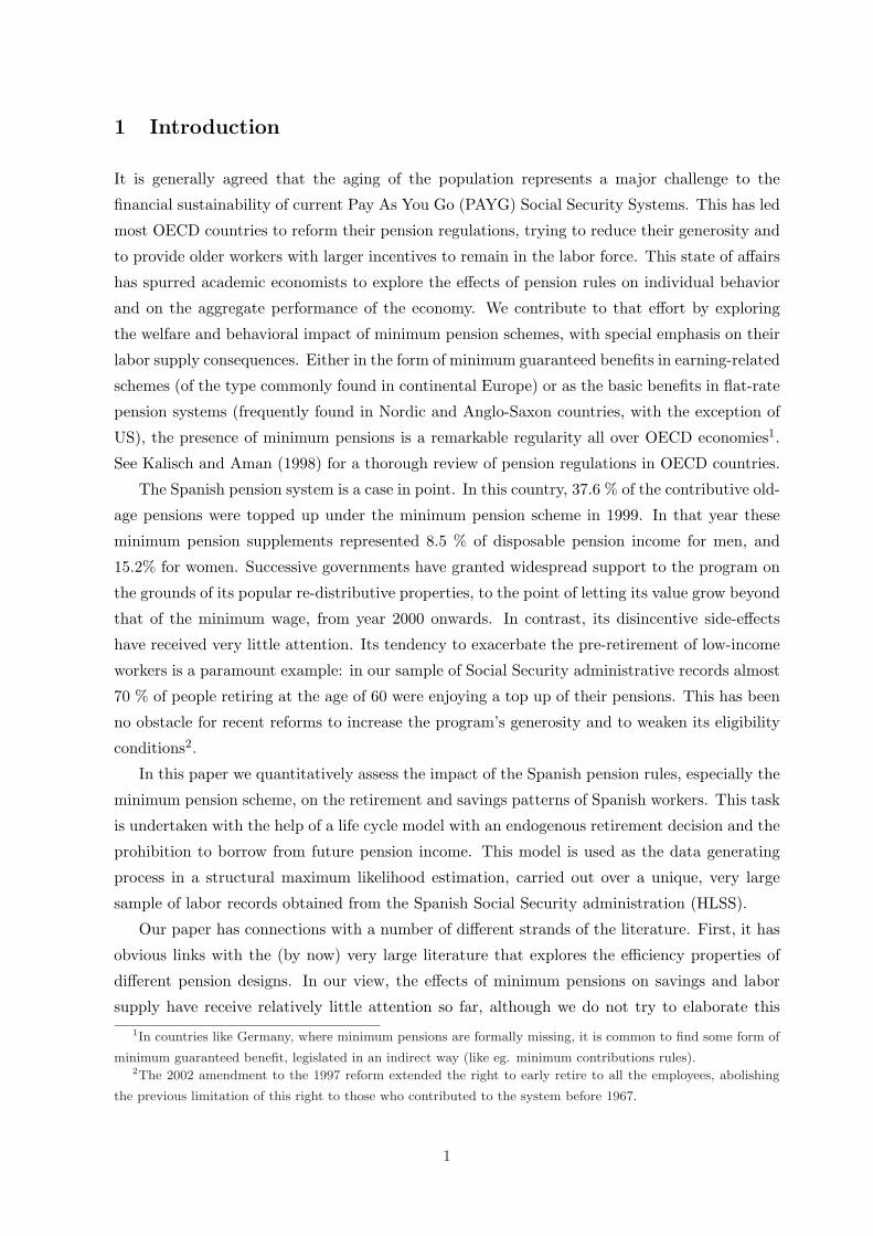
Figure 1: Minimum Pension for married individuals aged 65+ and Minimum Wage (“Salario Mınimo

Interprofesional”): log of real values in 1976–2004.

annually fixed by the government, has been very different: while maximum pensions have been

kept roughly constant in real terms over the last 15 years, minimum pensions have grown at

approximately the same rate as nominal wages. As a result of this policy, the minimum pension

(for married individuals aged 65+) is larger that the legislated Minimum Wage since 2000, and

that their values have continued to diverge ever since.

2.2 Labor supply patterns of older workers in Spain

Most Spanish workers withdraw from the labor force either at the ERA (60) or at the NRA

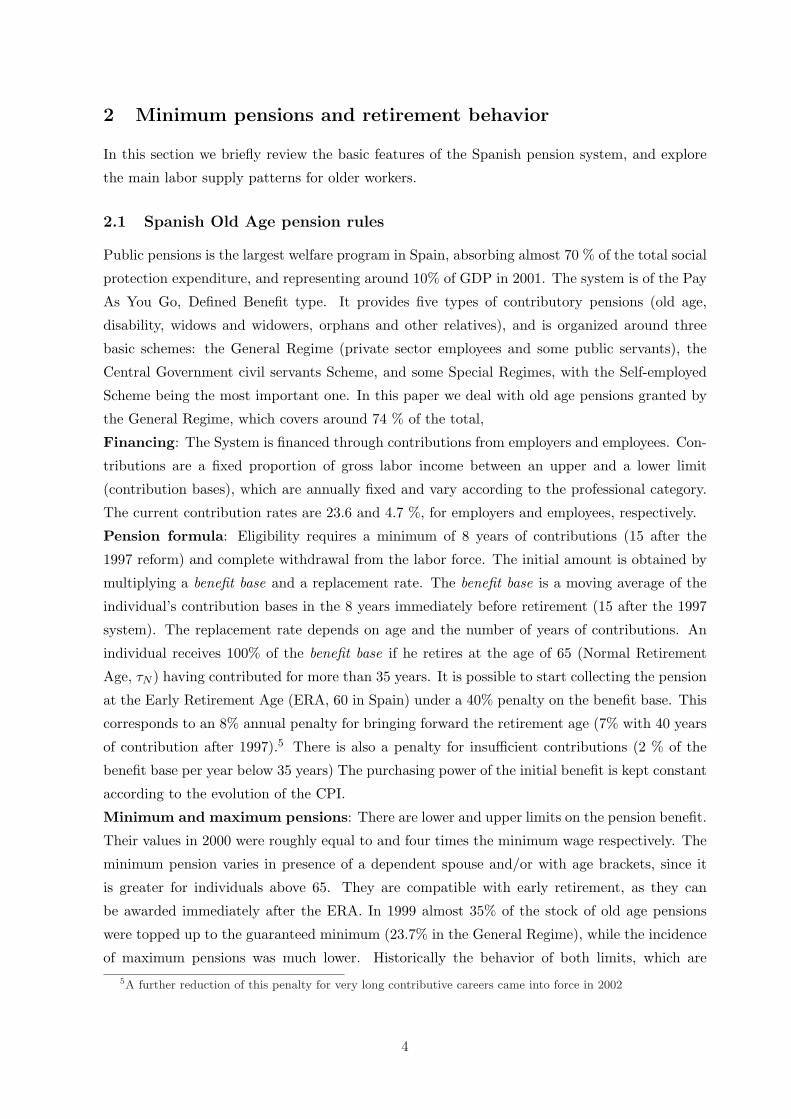
(65). This results in sharp discontinuities in the empirical retirement hazard at the pension

system’s key ages (figure 2). This is a very robust empirical pattern, shared by most countries

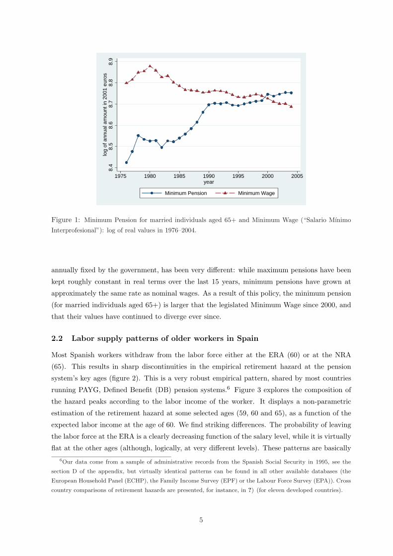
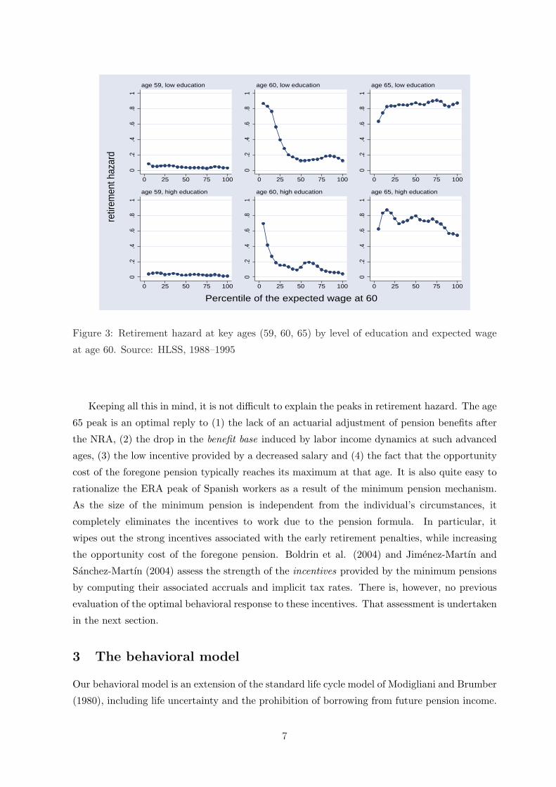
running PAYG, Defined Benefit (DB) pension systems.6 Figure 3 explores the composition of

the hazard peaks according to the labor income of the worker. It displays a non-parametric

estimation of the retirement hazard at some selected ages (59, 60 and 65), as a function of the

expected labor income at the age of 60. We find striking differences. The probability of leaving

the labor force at the ERA is a clearly decreasing function of the salary level, while it is virtually

flat at the other ages (although, logically, at very different levels). These patterns are basically6Our data come from a sample of administrative records from the Spanish Social Security in 1995, see the

section D of the appendix, but virtually identical patterns can be found in all other available databases (the

European Household Panel (ECHP), the Family Income Survey (EPF) or the Labour Force Survey (EPA)). Cross

country comparisons of retirement hazards are presented, for instance, in ?) (for eleven developed countries).

5

0.2

.4.6

.8re

tirem

ent h

azar

d

55 60 65 70age

sample hazard unaffected by MPaffected by MP

Figure 2: Retirement hazard by age in the full sample and in the subsamples of workerst that qualify

and fail-to-qualify for the minimum benefit (MP). Source: HLSS, 1995

independent of the educational achievement of the individual.7 It means that most early retirees

are low-income workers who qualify for a minimum pension top-up. We also find that 67.7% of

the people who retire at the exact age of 60 are actually receiving the minimum complement.

Finally, it is quite revealing that the retirement hazard at the age of 60 for those affected by the

minimum pension is 5 times larger than that for those who do not receive it (see figure 2).

An informal explanation of the empirical regularities

To explore the incentives underlying the pension regulations imagine a worker who decides to

stay working at a specific age τ . He faces two marginal disincentives for doing so: the reduction

in leisure time and, provided the eligibility conditions are met, the foregone pension benefit. On

the other hand, staying working allows the individual to collect a salary and implies a change in

the pension benefit he is entitled to in the future. This latter change depends on two elements.

Firstly, delaying retirement in the age range {τm, . . . , τN} reduces the early retirement penalty

(and the insufficient contributions penalty, if the number of years of contribution is lower than

35). Secondly, the benefit base changes as current gross labor income moves into the averaging

period and substitutes the value observed 8 years before (15 years under the 1997 system). Note

that while the first effect always results in higher benefits, the concavity of the life cycle profiles

of labor income can result in the second having the opposite effect.7The education level is not observable in our sample of social security records, but can be approximated by

the contribution group, with which the education level is highly correlated (see ?) for an illustration).

6

0.2

.4.6

.81

0 25 50 75 100

age 59, low education

0.2

.4.6

.81

0 25 50 75 100

age 60, low education

0.2

.4.6

.81

0 25 50 75 100

age 65, low education

0.2

.4.6

.81

0 25 50 75 100

age 59, high education

0.2

.4.6

.81

0 25 50 75 100

age 60, high education

0.2

.4.6

.81

0 25 50 75 100

age 65, high education

retir

emen

t haz

ard

Percentile of the expected wage at 60

Figure 3: Retirement hazard at key ages (59, 60, 65) by level of education and expected wage

at age 60. Source: HLSS, 1988–1995

Keeping all this in mind, it is not difficult to explain the peaks in retirement hazard. The age

65 peak is an optimal reply to (1) the lack of an actuarial adjustment of pension benefits after

the NRA, (2) the drop in the benefit base induced by labor income dynamics at such advanced

ages, (3) the low incentive provided by a decreased salary and (4) the fact that the opportunity

cost of the foregone pension typically reaches its maximum at that age. It is also quite easy to

rationalize the ERA peak of Spanish workers as a result of the minimum pension mechanism.

As the size of the minimum pension is independent from the individual’s circumstances, it

completely eliminates the incentives to work due to the pension formula. In particular, it

wipes out the strong incentives associated with the early retirement penalties, while increasing

the opportunity cost of the foregone pension. Boldrin et al. (2004) and Jimenez-Martın and

Sanchez-Martın (2004) assess the strength of the incentives provided by the minimum pensions

by computing their associated accruals and implicit tax rates. There is, however, no previous

evaluation of the optimal behavioral response to these incentives. That assessment is undertaken

in the next section.

3 The behavioral model

Our behavioral model is an extension of the standard life cycle model of Modigliani and Brumber

(1980), including life uncertainty and the prohibition of borrowing from future pension income.

7

This credit constraint is relevant in the absence of a bequest motive, an aspect first established

in Yaari (1965) and treated thoroughly in Leung (2000). We follow this latter paper in the

treatment of the model with a fixed retirement age, while our analysis of the retirement decision

is similar to that in Crawford and Lilien (1981) and Fabel (1994b).

Time in the model (ie, the age of the individual) is represented by t, while T stands for the

length of the individual life. T is a continuous random variable distributed on [t0, T ] according

to the survival function S(.) and mortality hazard h(.)8. The length of life is the only source

of uncertainty included in the model. We consider an individual of age t0 and study his/her

optimal decisions for what remains of the life-cycle. Their preferences for consumption, c(t) :

[t0, T ] → R+ and leisure, lτ (t) : [t0, T ] → [0, 1] (with lτ (t) = 1 ∀ t ∈ [τ, T ], ie. taking τ as the

age of full withdrawal from the labor force) are represented by a standard, additively separable

life-cycle utility function:

V (c, lτ , T ) =∫ T

t0e−δ (t−t0) υ(c(t), lτ (t)) dt

where δ is a discount factor. The period utility function is also additively separable in its two

arguments: υ(c, l) = u(c(t)) + ν(l(t)), with both components exhibiting the usual properties.9

Individuals choose the consumption path and the retirement age τ that maximize expected utility

under the constraints imposed by two market imperfections: the lack of an insurance market

for life uncertainty (i.e. the absence of private annuities) and the prohibition of borrowing from

future pension income (i.e., accumulated assets a(t) must not be negative after retirement in

order to avoid people dying with standing debts).

Working individuals receive a gross labor income w(t) and must pay social contributions

at a constant rate ς.10 After retirement, the consumer’s income consists of a flow of pension

benefits, b(t, τ), which depends on both age and the retirement age as discussed in section 2.1.

We also assume that there is no bequest motive for savings and that the public sector fully

taxes involuntary bequests. For the sake of simplicity we abstract from private pensions (quite

irrelevant in the Spanish case), work with a constant real interest rate, r, and take the life

cycle profile of labor hours l(t) as exogenously fixed. The formal statement of the intertemporal

problem is, then, as follows:8We assume that h(t) > 0 ∀[0, T ] and limt→T h(t) = ∞. Applying standard results it is easy to express

the survival function (conditional on being alive at the age of t0) as the non-linear discount function: S(t) =

exp(−

∫ t

t0h(s) ds

).

9They are twice continuously differentiable, strictly increasing and concave. We also assume that

limc→0 u′(c(t)) = ∞.10In this section we omit some of the institutional details to ease the exposition. For a complete record of the

institutional details we refer to table 1.

8

max E[V (c, l)] =∫ Tt0

e−δ (t−t0) S(t) [u(c(t)) + ν(lτ (t))] dt

c(t), a(t), τ st a(t) = r a(t) + w(t, τ)− c(t)

w(t, τ) = w(t)(1− ς) I(t0, τ) + b(t, τ) I(τ, T )

lτ (t) = l(t) I(t0, τ) + 1 I(τ, T )

a(t0) = a0 a(T ) = 0 a(t) ≥ 0 ∀ t ≥ τ

(1)

where I(t1, t2) is the indicator function for the event t ∈ [t1, t2].

Under the previous assumptions, the borrowing constraint always becomes binding before the

maximum life span (see proposition 1 in Leung (2000)). We denote this “wealth depletion time”

by t ∈ [τ , T ), where τ = max{τm, τ} (ie. the maximum between the ERA and the individual

retirement age). Following Crawford and Lilien (1981) and Fabel (1994b) we use this result to

transform the original constrained problem into a new un-constrained one including t as a new

decision variable.

max∫ tt0

e−δ(t)u(c(t)) dt +∫ Tt e−δ(t)u(b(t, τ)) dt +

∫ Tt0

e−δ(t)ν(lτ (t)) dt

c(t), τ, a(t), t st. a′(t) = r a(t) + w(t, τ)− c(t) t ∈ [t0, t]

w(t, τ) = w(t) (1− ς) I(t0, τ) + b(t, τ) I(τ, T )

t ∈ [τ , T ) lτ (t) = l(t) I(t0, τ) + 1 I(τ, T ) τ = max{τm, τ}a(t0) = a0 a(t) = 0 t ∈ [t, T ]

(2)

where eδ(t) is a shorthand notation for S(t) eδ (t−t0). We deal with this problem in three stages.

Firstly, we analytically characterize the optimal profiles of consumption and accumulated assets

for a given retirement age and a given binding age for the credit constraint. As this is a well

known step, we leave the algebraic details and a calibrated example to appendix A.1. Using

these conditional solutions we compute, in a second stage, the optimal binding age for any given

retirement age. Finally, we employ the information of the previous two stages to characterize

the optimal retirement age. A detailed discussion of the entire procedure is available in Jimenez-

Martın and Sanchez-Martın (2003).

3.1 Optimal retirement behavior

After the first two stages of our solution procedure we are left with the optimal unconditional

consumption function, cτ (t), and optimal binding age t(τ) for any fixed retirement age. We can

then characterize what the individual envisages as the optimal retirement behavior (given the

information available at age t0) as the solution to the static optimization problem:

maxτ∈[τ0,τ1]

E[V (cτ , lτ )] (3)

where t0 < τ0, τ1 < T and

E[V (cτ , lτ )] =∫ t(τ)

t0e−δ(t) u(cτ (t)) dt +

∫ T

t(τ)e−δ(t)u(b(t, τ)) dt +

∫ τ

t0ν(l(t)) dt +

∫ T

τν(1) dt

9

50 52 54 56 58 60 62 64 66 68 70−10

−5

0

5

10

15

λ e−r τ y’ − e−δ (τ) ∆ ν

λ e−r τ y’

Figure 4: Marginal utility of working by age for the Spanish median worker. We separately

show marginal changes in life cycle wealth λ e−r τ y′(τ), and the total marginal change implied,

including the impact of leisure reductions.

eδ(t) is a shorthand notation for S(t) eδ (t−t0). Some discontinuities introduced by the pension

regulations (see below) imply that V (τ) is only piecewise continuously differentiable. Therefore,

local optimum τ∗ can be either interior (d Vd τ (τ∗) = 0 and d 2 V

d τ 2 (τ∗) < 0), or corner solutions, i.e.,

ages where the marginal utility of working changes its sign in a discrete, negative drop. Therefore,

finding the best retirement age involves a comparison among the utility levels achieved in local

optima and corner solutions.

In our life cycle context, the optimal retirement is driven by a relatively simple income/leisure

trade-off. This can be shown by exploring the marginal utility of staying employed at age τ :d V

d τ(τ) = λ e−r (τ−t0) y′(τ)− e−δ(τ) ∆ ν(τ) (4)

where λ is the lagrange multiplier associated with the implicit Intertemporal Budget Constraint,

y′(τ) is the current value of the marginal changes in τ -conditional life cycle wealth, and

∆ ν(τ) = ν(1)− ν(lτ ) (5)

is the current utility cost of the foregone leisure. Note that pension rules have a critical influence

on retirement by shaping the evolution of y′(.) with the retirement age, as we review in the next

section.

3.2 The effects of pension rules on individual behavior

By staying in the workforce at age τ , the individual’s life cycle wealth is modified in three

different ways. On the one hand, current income takes the form of labor earnings, with the

10

reception of pension benefits being deferred for at least one period (assuming the individual

meets the eligibility criteria). On the other hand, the pension benefit the worker is entitled to

receive in the future changes. This latter effect can be very important, as it alters the income

to be perceived at every single year after retirement. The analytical expression of these changes

is given by:

y′(τ) = w(τ)(1− ς)− b I(τ ≥ τm) + b′ A(τ , t) (6)

where I(.) is a standard indicator function and A(τ , t) captures the effect, accumulated over the

individual’s entire remaining life, of marginal changes in the benefit:

A(τ , t) =∫ t

τe−r(t−τ) dt + e−r(t−τ)

∫ T

te−(δ(t)−δ(t)) dt

The first term represents the impact along the interior optimal consumption path, while the

second captures the direct impact of changes in b in the utility function after the optimal wealth

depletion age.11

Notice that the second term vanishes under perfect capital markets. The trade off is slightly

different in the presence of corner solutions, i.e. when cτ (τ | τ) < b(τ). However, as this is not a

very common situation, we have confined the details to appendix B, where a general expression

for the marginal utility of working is presented.

The incentives the pension rules create for an average Spanish worker (characterized by a

concave wage profile) are displayed in figure 4 and can be summarized as follows:

• Before the ERA, τm, workers have very significant incentives to keep working, stemming

basically from a relatively high salary and the fact that they do not suffer the marginal

cost of the foregone pension (this is revealed by the indicator function, I(τ ≥ τm), in (6)).

• In the age range [τm, τN ) individuals have strong incentives to keep working. This is a

direct consequence of the early retirement penalties: by staying employed, individuals are

granted the equivalent of an 8% annual increase in the replacement rate. This more than

offsets the opportunity cost of the foregone pension, resulting in a positive jump in the

marginal utility of working along this time interval.

• Once the individual reaches the NRA, that is, when there are no further premia for delaying

retirement, the incentive to work vanishes (recall the arguments given in section 2.2)

11 Equation (6) is obtained from the first term of d V/d τ in (4) (the component derived from changes in

consumption):

λ e−r (τ−t0)

[w(τ)(1− ς)− b I(τ ≥ τm) + b′(τ)

∫ t

τ

e−r (t−τ) dt

]+ b′(τ)

∫ T

t

e−δ(t) u′(b) dt

by using the first order condition for optimal consumption e−δ(t)u′(c(t)) = λ e−r(t−t0) and recalling that c(t) = b.

11

50 55 60 65 7012

14

16

18

20

22λ

50 55 60 65 70−0.5

0

0.5

1

1.5

2

2.5Y’

50 55 60 65 70−2

0

2

4

6

8

10

12

50 55 60 65 70−10

−5

0

5

10λ e−r τ y’ − e−δ (τ) ∆ νλ e−r τ y’

min pension

min pension

min pension min pension

Figure 5: Income and substitution effects induced by the minimum pension scheme on a worker

in the 10th quantile of the income distribution.

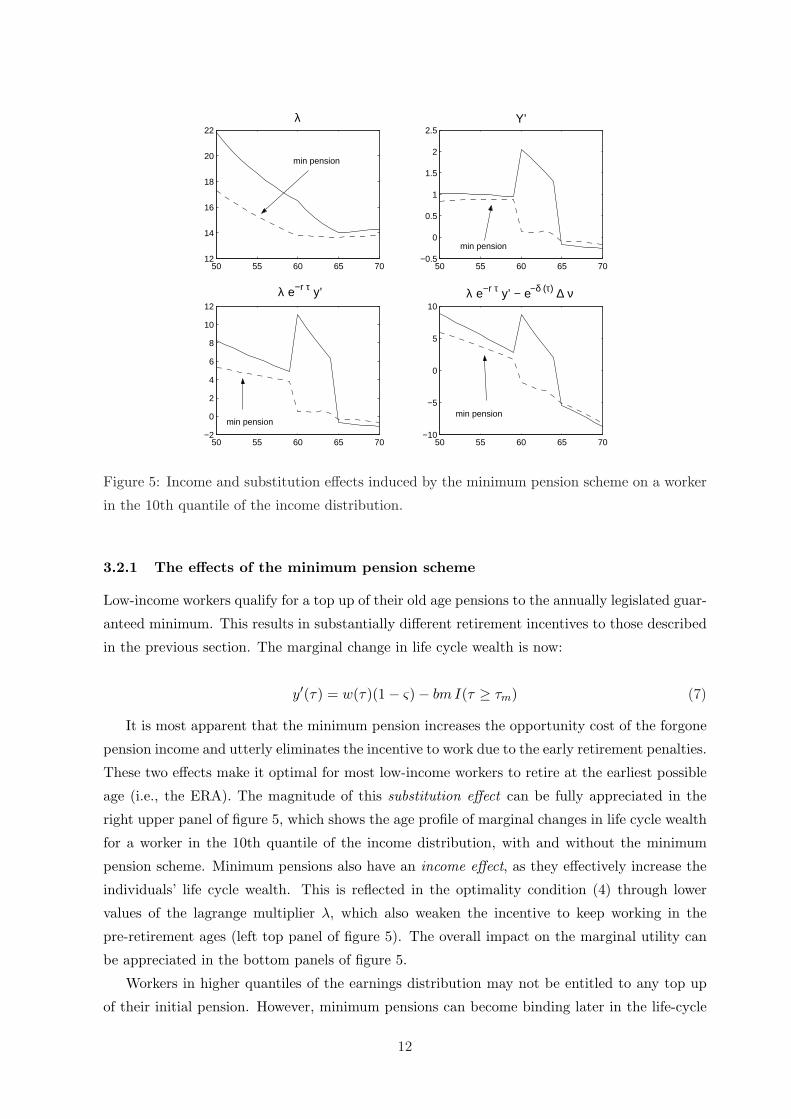
3.2.1 The effects of the minimum pension scheme

Low-income workers qualify for a top up of their old age pensions to the annually legislated guar-

anteed minimum. This results in substantially different retirement incentives to those described

in the previous section. The marginal change in life cycle wealth is now:

y′(τ) = w(τ)(1− ς)− bm I(τ ≥ τm) (7)

It is most apparent that the minimum pension increases the opportunity cost of the forgone

pension income and utterly eliminates the incentive to work due to the early retirement penalties.

These two effects make it optimal for most low-income workers to retire at the earliest possible

age (i.e., the ERA). The magnitude of this substitution effect can be fully appreciated in the

right upper panel of figure 5, which shows the age profile of marginal changes in life cycle wealth

for a worker in the 10th quantile of the income distribution, with and without the minimum

pension scheme. Minimum pensions also have an income effect, as they effectively increase the

individuals’ life cycle wealth. This is reflected in the optimality condition (4) through lower

values of the lagrange multiplier λ, which also weaken the incentive to keep working in the

pre-retirement ages (left top panel of figure 5). The overall impact on the marginal utility can

be appreciated in the bottom panels of figure 5.

Workers in higher quantiles of the earnings distribution may not be entitled to any top up

of their initial pension. However, minimum pensions can become binding later in the life-cycle

12

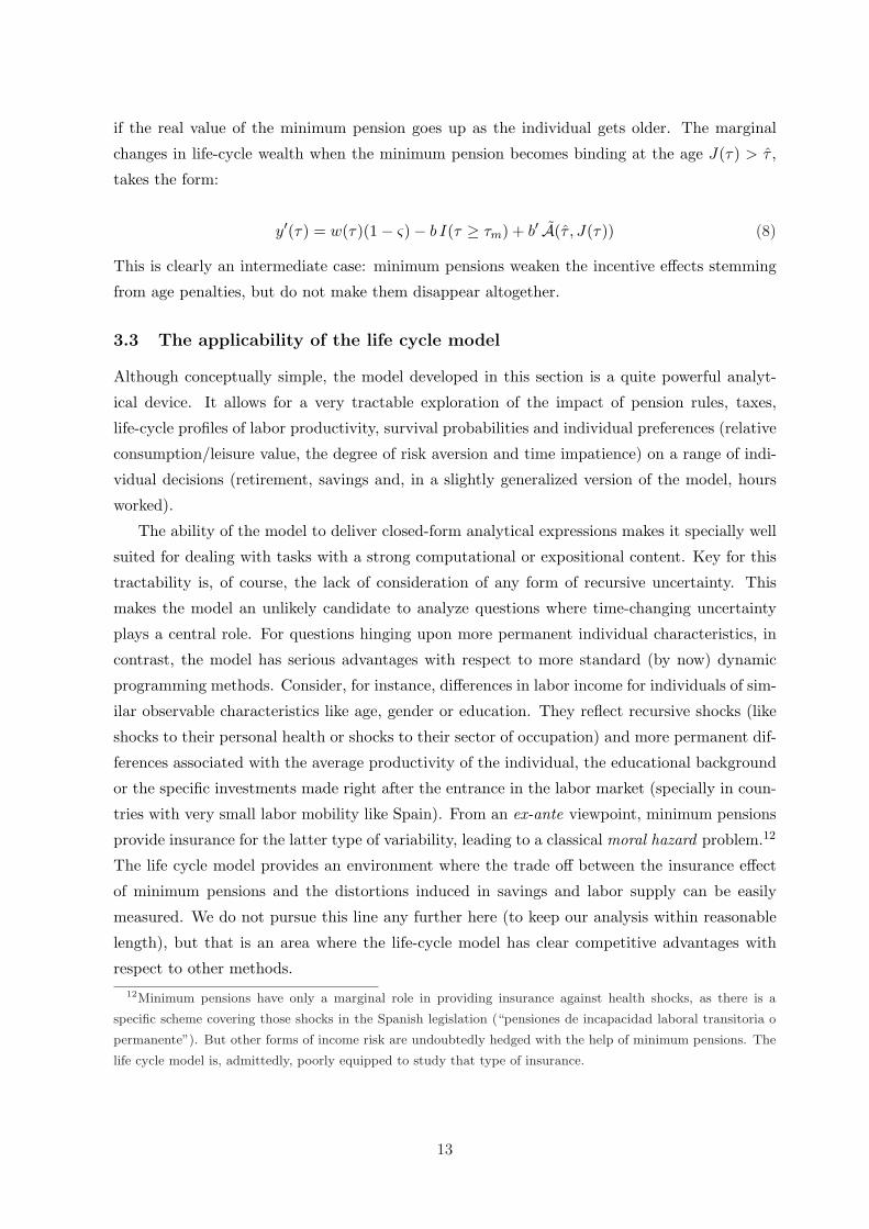
if the real value of the minimum pension goes up as the individual gets older. The marginal

changes in life-cycle wealth when the minimum pension becomes binding at the age J(τ) > τ ,

takes the form:

y′(τ) = w(τ)(1− ς)− b I(τ ≥ τm) + b′ A(τ , J(τ)) (8)

This is clearly an intermediate case: minimum pensions weaken the incentive effects stemming

from age penalties, but do not make them disappear altogether.

3.3 The applicability of the life cycle model

Although conceptually simple, the model developed in this section is a quite powerful analyt-

ical device. It allows for a very tractable exploration of the impact of pension rules, taxes,

life-cycle profiles of labor productivity, survival probabilities and individual preferences (relative

consumption/leisure value, the degree of risk aversion and time impatience) on a range of indi-

vidual decisions (retirement, savings and, in a slightly generalized version of the model, hours

worked).

The ability of the model to deliver closed-form analytical expressions makes it specially well

suited for dealing with tasks with a strong computational or expositional content. Key for this

tractability is, of course, the lack of consideration of any form of recursive uncertainty. This

makes the model an unlikely candidate to analyze questions where time-changing uncertainty

plays a central role. For questions hinging upon more permanent individual characteristics, in

contrast, the model has serious advantages with respect to more standard (by now) dynamic

programming methods. Consider, for instance, differences in labor income for individuals of sim-

ilar observable characteristics like age, gender or education. They reflect recursive shocks (like

shocks to their personal health or shocks to their sector of occupation) and more permanent dif-

ferences associated with the average productivity of the individual, the educational background

or the specific investments made right after the entrance in the labor market (specially in coun-

tries with very small labor mobility like Spain). From an ex-ante viewpoint, minimum pensions

provide insurance for the latter type of variability, leading to a classical moral hazard problem.12

The life cycle model provides an environment where the trade off between the insurance effect

of minimum pensions and the distortions induced in savings and labor supply can be easily

measured. We do not pursue this line any further here (to keep our analysis within reasonable

length), but that is an area where the life-cycle model has clear competitive advantages with

respect to other methods.12Minimum pensions have only a marginal role in providing insurance against health shocks, as there is a

specific scheme covering those shocks in the Spanish legislation (“pensiones de incapacidad laboral transitoria o

permanente”). But other forms of income risk are undoubtedly hedged with the help of minimum pensions. The

life cycle model is, admittedly, poorly equipped to study that type of insurance.

13

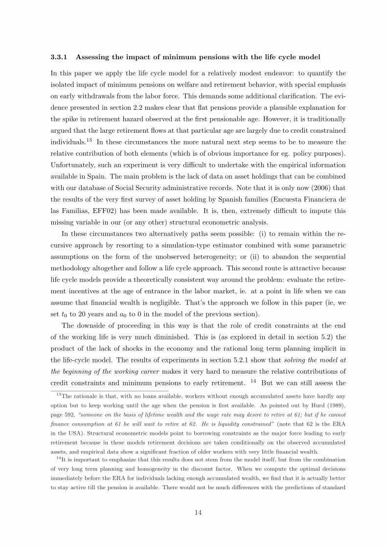
3.3.1 Assessing the impact of minimum pensions with the life cycle model

In this paper we apply the life cycle model for a relatively modest endeavor: to quantify the

isolated impact of minimum pensions on welfare and retirement behavior, with special emphasis

on early withdrawals from the labor force. This demands some additional clarification. The evi-

dence presented in section 2.2 makes clear that flat pensions provide a plausible explanation for

the spike in retirement hazard observed at the first pensionable age. However, it is traditionally

argued that the large retirement flows at that particular age are largely due to credit constrained

individuals.13 In these circumstances the more natural next step seems to be to measure the

relative contribution of both elements (which is of obvious importance for eg. policy purposes).

Unfortunately, such an experiment is very difficult to undertake with the empirical information

available in Spain. The main problem is the lack of data on asset holdings that can be combined

with our database of Social Security administrative records. Note that it is only now (2006) that

the results of the very first survey of asset holding by Spanish families (Encuesta Financiera de

las Familias, EFF02) has been made available. It is, then, extremely difficult to impute this

missing variable in our (or any other) structural econometric analysis.

In these circumstances two alternatively paths seem possible: (i) to remain within the re-

cursive approach by resorting to a simulation-type estimator combined with some parametric

assumptions on the form of the unobserved heterogeneity; or (ii) to abandon the sequential

methodology altogether and follow a life cycle approach. This second route is attractive because

life cycle models provide a theoretically consistent way around the problem: evaluate the retire-

ment incentives at the age of entrance in the labor market, ie. at a point in life when we can

assume that financial wealth is negligible. That’s the approach we follow in this paper (ie, we

set t0 to 20 years and a0 to 0 in the model of the previous section).

The downside of proceeding in this way is that the role of credit constraints at the end

of the working life is very much diminished. This is (as explored in detail in section 5.2) the

product of the lack of shocks in the economy and the rational long term planning implicit in

the life-cycle model. The results of experiments in section 5.2.1 show that solving the model at

the beginning of the working career makes it very hard to measure the relative contributions of

credit constraints and minimum pensions to early retirement. 14 But we can still assess the13The rationale is that, with no loans available, workers without enough accumulated assets have hardly any

option but to keep working until the age when the pension is first available. As pointed out by Hurd (1989),

page 592, “someone on the basis of lifetime wealth and the wage rate may desire to retire at 61; but if he cannot

finance consumption at 61 he will wait to retire at 62. He is liquidity constrained” (note that 62 is the ERA

in the USA). Structural econometric models point to borrowing constraints as the major force leading to early

retirement because in these models retirement decisions are taken conditionally on the observed accumulated

assets, and empirical data show a significant fraction of older workers with very little financial wealth.14It is important to emphasize that this results does not stem from the model itself, but from the combination

of very long term planning and homogeneity in the discount factor. When we compute the optimal decisions

immediately before the ERA for individuals lacking enough accumulated wealth, we find that it is actually better

to stay active till the pension is available. There would not be much differences with the predictions of standard

14

incidence of early retirement with and without the minimum pension and check the robustness

of our findings. More precisely, our main experiment in this paper is as follows. We first extend

the life-cycle model by considering one simple form of unobserved heterogeneity (the individual

value of leisure); We then use the resulting probabilistic model as the data generating process

for the estructural estimation of the preference parameters in the model; Finally, we compute

how much early retirement is generated by the minimum pension in the life-cycle model (section

5.1). The robustness of these findings to the indirect omission of the impact of credit constraints

is tested via simulations in section 5.2.

4 Econometric estimation of the preference parameters

In this section we design a method to recover the preference parameters by comparing optimal

retirement (as predicted by the previous section’s theoretical model) with actual retirement

data (from our HLSS database, which is described in appendix D). We start by reporting

the way we introduce variability in individual retirement ages, by assuming a specific form of

unobserved heterogeneity in the population. We then describe the details of our maximum

likelihood estimation procedure, present the results obtained and discuss their implications.

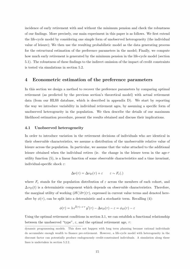
4.1 Unobserved heterogeneity

In order to introduce variation in the retirement decisions of individuals who are identical in

their observable characteristics, we assume a distribution of the unobservable relative value of

leisure across the population. In particular, we assume that the value attached to the additional

leisure obtained when the individual retires (ie. the change in the leisure term in the age-τ

utility function (5), is a linear function of some observable characteristics and a time invariant,

individual-specific shock ε:

∆ν(τ) = ∆νD(τ) + ε ε ∼ Fε(.)

where Fε stands for the population distribution of ε across the members of each cohort, and

∆ νD(t) is a deterministic component which depends on observable characteristics. Therefore,

the marginal utility of working (∂V/∂τ)(τ), expressed in current value terms and denoted here-

after by φ(τ), can be split into a deterministic and a stochastic term. Recalling (4):

φ(τ) = λ eδ(τ)−r τ y′(τ)−∆νD(τ)− ε = φD(τ)− ε

Using the optimal retirement conditions in section 3.1, we can establish a functional relationship

between the unobserved “type”, ε, and the optimal retirement age, τ :

dynamic programming models. This does not happen with long term planning because rational individuals

do accumulate enough wealth to finance pre-retirement. However, a life-cycle model with heterogeneity in the

discount factor can potentially produce endogenously credit-constrained individuals. A simulation along these

lines is undertaken in section 5.2.2.

15

ε = φ∗D(τ)

The asterisk reminds us of the need for discarding local optima in order to have a one-to-one

relationship between the two variables. Note that individuals with different observable charac-

teristics will have different age profiles of φ∗D. Finally, a change of variable in the distribution

function of ε leads to a (conditional on the observables) distribution law for the stochastic

optimal retirement age. The unconditional probability of being retired at age t or before is then:

Fτ (t) = P [τ ≤ t] = P [φ∗−1

D (ε) ≤ t] = P [ε ≥ φ∗D(t)] = 1− Fε(φ∗D(t)) (9)

This continuous-time specification becomes operative by making τ discrete and considering

the existence of lower and upper limits in the retirement age (τ and τ respectively). Then, from

the viewpoint of the analyst, retirement is a discrete stochastic variable ξ ∈ {τ , τ + 1, . . . , τ},distributed according to the following law:

Fξ(a) =

1− Fε(φ∗D(τ)) a = τ

1− Fε(φ∗D(a)) a ∈ {τ + 1, . . . , τ − 1}Fε(φ∗D(τ)) a = τ

(10)

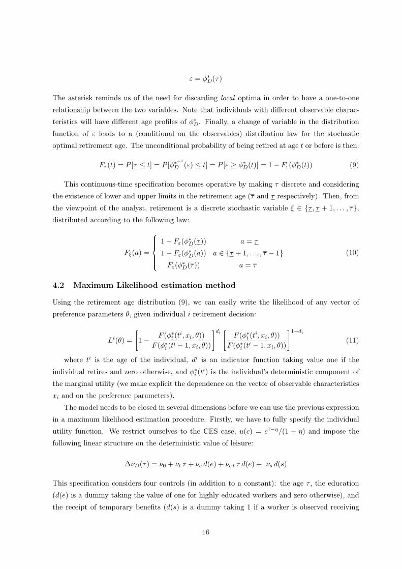
4.2 Maximum Likelihood estimation method

Using the retirement age distribution (9), we can easily write the likelihood of any vector of

preference parameters θ, given individual i retirement decision:

Li(θ) =

[1− F (φ∗i (t

i, xi, θ))F (φ∗i (ti − 1, xi, θ))

]di[

F (φ∗i (ti, xi, θ))

F (φ∗i (ti − 1, xi, θ))

]1−di

(11)

where ti is the age of the individual, di is an indicator function taking value one if the

individual retires and zero otherwise, and φ∗i (ti) is the individual’s deterministic component of

the marginal utility (we make explicit the dependence on the vector of observable characteristics

xi and on the preference parameters).

The model needs to be closed in several dimensions before we can use the previous expression

in a maximum likelihood estimation procedure. Firstly, we have to fully specify the individual

utility function. We restrict ourselves to the CES case, u(c) = c1−η/(1 − η) and impose the

following linear structure on the deterministic value of leisure:

∆νD(τ) = ν0 + νt τ + νe d(e) + νe t τ d(e) + νs d(s)

This specification considers four controls (in addition to a constant): the age τ , the education

(d(e) is a dummy taking the value of one for highly educated workers and zero otherwise), and

the receipt of temporary benefits (d(s) is a dummy taking 1 if a worker is observed receiving

16

temporary benefits, either related to unemployment or to illness). We also allow for an interac-

tion term between age and education. Consequently, the vector of the preference parameters to

be estimated is θ = (ν0, νe, νe t, νt, νs, δ, η).

Secondly, we have to specify the economic environment, including the institutional setting,

the wage process, the interest rate, the survival process, the heterogeneity dimensions and their

population distributions. All these elements are specified as follows:

• The permanent component of the relative value of leisure, ε, is assumed to be normally

distributed across individuals: ε ∼ N(0, 1). This introduces some similarities between our

empirical model and a reduced form probit model. Note, however, that our unobservable

individual type ε is permanent rather than the annual shock included in the probit case.

This accounts for the non standard denominator in our likelihood function (11).

Table 1: Stylized version of the Spanish RGSS pension rules. 1985 system.Provision Expression Definitions

τm is the ERAElegibility τ ≥ τm = 60 a(τ) ≥ 15 a(.) denotes

years of contributionscx, cm are respectively the

Covered wages c(t) = min{cx(t),max{w(t), cm(t)} } Max and Min. covered wagec(t) denotes contributionsw(τ) is the benefit base

Benefit Base w(τ) = (1/R)∑τ

τ−R c(t) dt R: length of the averagingperiod (8 in 1995)

Age Penalty α(τ) =

α0 if τ < τm

α0 + α1(τ − τm) if τm ≤ τ ≤ τN

1 otherwise

τN is the NRAα0 = .60α1 = .08

History Penalty κ(a(τ)) =

κ0 if a(τ) < 15κ0 + κ1(a(τ)− am) if 15 ≤ a(τ) ≤ 35

1 otherwiseκ0 = .60κ1 = .02

b(t, τ) is the pre-tax pensionPension b(t, τ) = min{bx(t),max{α(τ) κ(a(τ)) w(τ), bm(t, τ)} } bx is the maximum pension

bm is the minimum pensionFurther Maximum contributions and pensions are constant in real termsassumptions The minimum pension real growth rate or generosity is 0.5 %.

• We assume all individuals in the sample share the same survival probabilities, estimated

from the 1995, National Statistics Institute (INE) mortality data.

• We include in our simulations a stylized version of the pension rules in the Spanish General

Regime. The parameter values are those in effect before the 1997 reform (the estimation

sample is the 1995 cross section of HLSS). These values are presented in Table 1.

We implement the estimation procedure in three economies of increasing institutional

complexity. The first one, E1, only includes the pension rules relevant for the “average”

individual (i.e.; it excludes the upper and lower limits on both pensions and contributions).

17

On top of this we consider a second economy, E2, in which there is a minimum guaranteed

income level (bm) available for workers older than the ERA. We refer to the rate of real

growth of the minimum pension as the generosity of the system. Finally, on the top

of E2 we specify the economy E3, in which there is a unique maximum pension, and a

minimum and maximum level of contributions, which vary across individuals according to

their professional qualification. The comparison of the results under E2 and E3 will allow

us to evaluate the marginal contribution of this last group of pension rules in explaining

the empirical retirement patterns.

• The base value for our constant interest rate is 3%.

• The other components of the vector of observable information xi (wages, education and

labor history) are used to compute the marginal utility φ∗(ti) for every individual in the

sample. The key part for this task is to construct, for each individual in the sample,

a smoothed life-cycle profile of labor earnings compatible with the observed information

from 1986 to 1995. This is crucial in estimating the wages, pensions and wealth of each

individual in the sample. The details are provided in appendix D and further explained

in Boldrin et al. (2004).

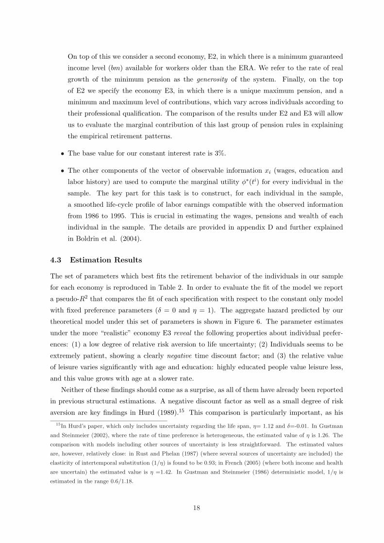
4.3 Estimation Results

The set of parameters which best fits the retirement behavior of the individuals in our sample

for each economy is reproduced in Table 2. In order to evaluate the fit of the model we report

a pseudo-R2 that compares the fit of each specification with respect to the constant only model

with fixed preference parameters (δ = 0 and η = 1). The aggregate hazard predicted by our

theoretical model under this set of parameters is shown in Figure 6. The parameter estimates

under the more “realistic” economy E3 reveal the following properties about individual prefer-

ences: (1) a low degree of relative risk aversion to life uncertainty; (2) Individuals seems to be

extremely patient, showing a clearly negative time discount factor; and (3) the relative value

of leisure varies significantly with age and education: highly educated people value leisure less,

and this value grows with age at a slower rate.

Neither of these findings should come as a surprise, as all of them have already been reported

in previous structural estimations. A negative discount factor as well as a small degree of risk

aversion are key findings in Hurd (1989).15 This comparison is particularly important, as his15In Hurd’s paper, which only includes uncertainty regarding the life span, η= 1.12 and δ=-0.01. In Gustman

and Steinmeier (2002), where the rate of time preference is heterogeneous, the estimated value of η is 1.26. The

comparison with models including other sources of uncertainty is less straightforward. The estimated values

are, however, relatively close: in Rust and Phelan (1987) (where several sources of uncertainty are included) the

elasticity of intertemporal substitution (1/η) is found to be 0.93; in French (2005) (where both income and health

are uncertain) the estimated value is η =1.42. In Gustman and Steinmeier (1986) deterministic model, 1/η is

estimated in the range 0.6/1.18.

18

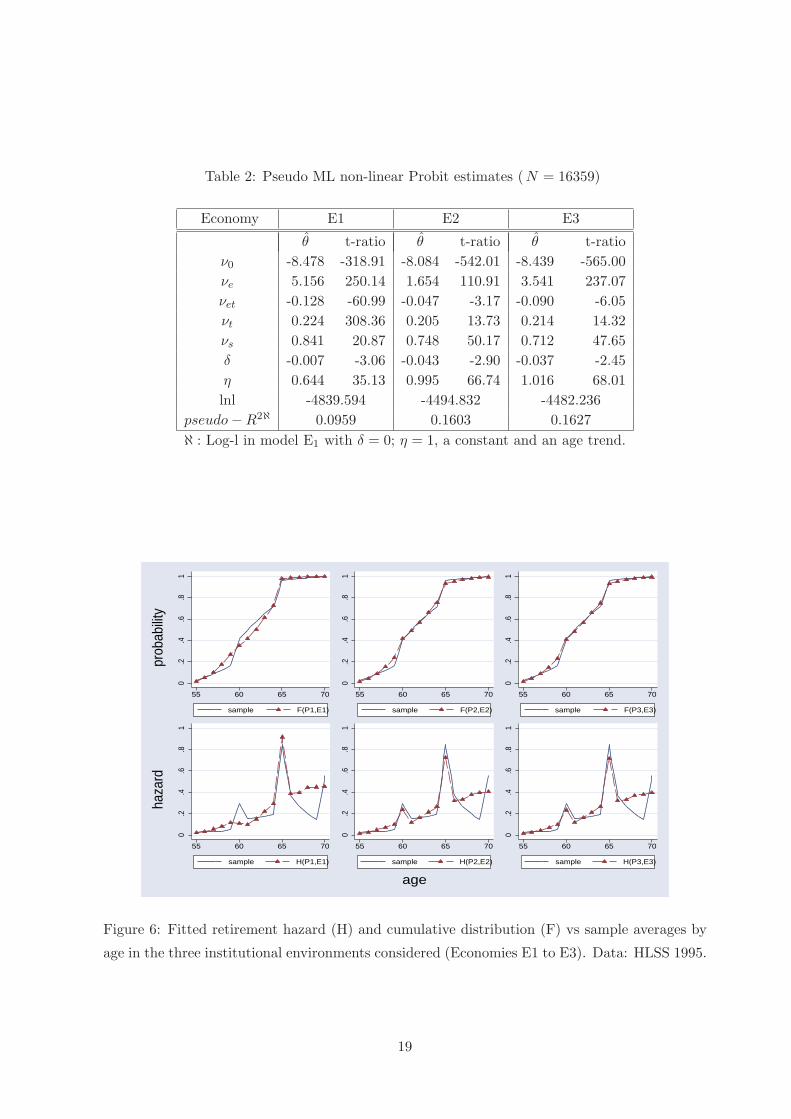
Table 2: Pseudo ML non-linear Probit estimates (N = 16359)

Economy E1 E2 E3

θ t-ratio θ t-ratio θ t-ratioν0 -8.478 -318.91 -8.084 -542.01 -8.439 -565.00νe 5.156 250.14 1.654 110.91 3.541 237.07νet -0.128 -60.99 -0.047 -3.17 -0.090 -6.05νt 0.224 308.36 0.205 13.73 0.214 14.32νs 0.841 20.87 0.748 50.17 0.712 47.65δ -0.007 -3.06 -0.043 -2.90 -0.037 -2.45η 0.644 35.13 0.995 66.74 1.016 68.01lnl -4839.594 -4494.832 -4482.236

pseudo−R2ℵ 0.0959 0.1603 0.1627ℵ : Log-l in model E1 with δ = 0; η = 1, a constant and an age trend.

0.2

.4.6

.81

55 60 65 70

sample F(P1,E1)

0.2

.4.6

.81

55 60 65 70

sample F(P2,E2)

0.2

.4.6

.81

55 60 65 70

sample F(P3,E3)

0.2

.4.6

.81

55 60 65 70

sample H(P1,E1)

0.2

.4.6

.81

55 60 65 70

sample H(P2,E2)

0.2

.4.6

.81

55 60 65 70

sample H(P3,E3)

haz

ard

p

roba

bilit

y

age

Figure 6: Fitted retirement hazard (H) and cumulative distribution (F) vs sample averages by

age in the three institutional environments considered (Economies E1 to E3). Data: HLSS 1995.

19

estimations are obtained from a life-cycle model which is very close to ours. The main difference

is that Hurd’s results stem from the model’s predictions about optimal savings, while ours come

from the implications of the model in terms of optimal retirement. In Hurd’s paper, a negative

δ helps the model to reproduce the observed amounts of accumulated assets at advanced ages.

In our work the degree of time impatience determines the sign and magnitude of the incentives

provided by the pension regulations. Very patient workers value the financial gains stemming

from delayed retirement a great deal. This keeps them active until the NRA, unless minimum

pensions block this incentive. Therefore, a negative δ emerges in our estimations as a form to

express the high attachment to the labor force shown by average and above average Spanish

wage-earners.

Highly educated workers usually have better working conditions and more pleasant occupa-

tions, which result in a higher attachment to activity. Our extremely stylized model has only one

way to reflect these facts: by lowering the estimated relative value of leisure for these workers.

On the other hand, a pattern of strong increase in leisure value as individuals grow older is quite

common in the literature (see for instance Gustman and Steinmeier (1986)).

The adjustment of the model

The life cycle approach is well suited to our purpose of exploring the incentives provided by

the pension regulation, but it is far from being a complete theory of retirement. It is clear

that recursive models may provide a more comprehensive ground for empirical analysis. The

estimation of our life cycle model is, however, a very valuable experiment as it gives us a set

of parameters values that are fully consistent with our theoretical model. Furthermore, the

estimation gives a chance to test the empirical performance of the life cycle theory. This is

summarized in the third column of Figure 6, where the estimated cumulative distribution and

hazard by age are compared to their empirical counterparts.

Loosely speaking, the life cycle model does a rather satisfactory job at reproducing the

empirical retirement distribution. Summing up, we observe that our base model (E3): (1) slightly

overestimates retirement flows immediately before 60; (2) reproduces a spike in retirement flows

at 60, but its size is a bit lower than that in the data; (3) overstates the number of people

retiring immediately before the Normal retirement age; and, finally, generates a large spike at

the NRA, although, again, it is of a smaller magnitude than the empirical one. The relatively

high post-65 hazards found are entirely due to the very small predicted probability of survival

in the labor force beyond the NRA. The probability of retirement at those ages is actually very

small and decreasing.

That we do not fully reproduce the size of the peaks is easy to understand as some rele-

vant economic processes are missed in our stylized life-cycle model. First, there is no health

uncertainty or unemployment shocks. Clearly, both factors can contribute to the age 60 spike:

Individuals who receive mild health shocks at any age before 60 and fail to qualify for a disability

20

pension may well decide to keep working till the retirement benefit first becomes available. A

similar story could be applied to people who have been fired before 60: they could stay active

claiming the unemployment benefit and start collecting the pension as soon as possible. The

underestimation of the age 65 peak could stem from the combination of institutional factors (col-

lective agreement clauses) and firms decisions. In absence of these elements, our model tends to

shift some of the retirement flows from the NRA to the ages immediately before 65.

From our sequence of simulations (E1 to E3) we extract two relevant implications. Firstly,

the comparison between E1 and E2 confirms that the economy without minimum pensions (E1)

is utterly incapable of reproducing the empirical patterns of pre-retirement (withdrawals before

or at the ERA) and early retirement (before 65). And, secondly, the coincidence between the

estimated hazard for economies E2 and E3 identifies the minimum pension as the key factor

shaping early retirement patterns, and play down the role of maximum pension and min/max

of contributions.

We showed in section 2.2 that the age-60 retirement peak is basically due to the behavior of

low income workers. To test the ability of the model to reproduce this observation we compare

in figure 7 the retirement hazard by age in the data and in the model, for three wage groups (de-

limited by the 1/3 and 2/3 quantiles of earnings: 1.58 and 2.60 million pesetas respectively). We

can appreciate how the life cycle model (once equipped with the minimum pension mechanism)

successfully reproduces this empirical regularity.

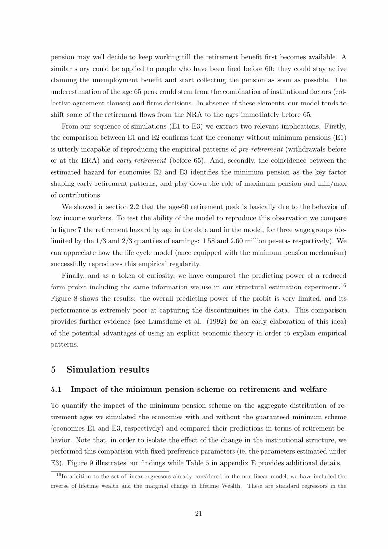
Finally, and as a token of curiosity, we have compared the predicting power of a reduced

form probit including the same information we use in our structural estimation experiment.16

Figure 8 shows the results: the overall predicting power of the probit is very limited, and its

performance is extremely poor at capturing the discontinuities in the data. This comparison

provides further evidence (see Lumsdaine et al. (1992) for an early elaboration of this idea)

of the potential advantages of using an explicit economic theory in order to explain empirical

patterns.

5 Simulation results

5.1 Impact of the minimum pension scheme on retirement and welfare

To quantify the impact of the minimum pension scheme on the aggregate distribution of re-

tirement ages we simulated the economies with and without the guaranteed minimum scheme

(economies E1 and E3, respectively) and compared their predictions in terms of retirement be-

havior. Note that, in order to isolate the effect of the change in the institutional structure, we

performed this comparison with fixed preference parameters (ie, the parameters estimated under

E3). Figure 9 illustrates our findings while Table 5 in appendix E provides additional details.16In addition to the set of linear regressors already considered in the non-linear model, we have included the

inverse of lifetime wealth and the marginal change in lifetime Wealth. These are standard regressors in the

21

0.2

.4.6

.81

55 60 65 70

sample H(P1,E1)

0.2

.4.6

.81

55 60 65 70

sample H(P2,E2)

0.2

.4.6

.81

55 60 65 70

sample H(P3,E3)

0.2

.4.6

.81

55 60 65 70

sample H(P1,E1)0

.2.4

.6.8

1

55 60 65 70

sample H(P2,E2)

0.2

.4.6

.81

55 60 65 70

sample H(P3,E3)

0.2

.4.6

.81

55 60 65 70

sample H(P1,E1)

0.2

.4.6

.81

55 60 65 70

sample H(P2,E2)

0.2

.4.6

.81

55 60 65 70

sample H(P3,E3)

retir

emen

t haz

ard

age

Figure 7: Retirement hazard by age and wage level in the three institutional environments

considered (Economies E1 to E3). The wage levels (W1 to W3) are delimited by the percentiles

1/3 and 2/3 of the empirical distribution. Data: HLSS 1995.

0.2

5.5

.75

1re

tirem

ent h

azar

d

55 60 65 70age

sample hazard est. probit hazard

Figure 8: Hazard out of the labor force: sample vs. predictions form a probit model using the

same information as our estructural model. Data: HLSS 1995.

22

0.0

0.1

0.1

0.1

0.2

0.3

retir

emen

t den

sity

55 60 65 70age

with MP without MP

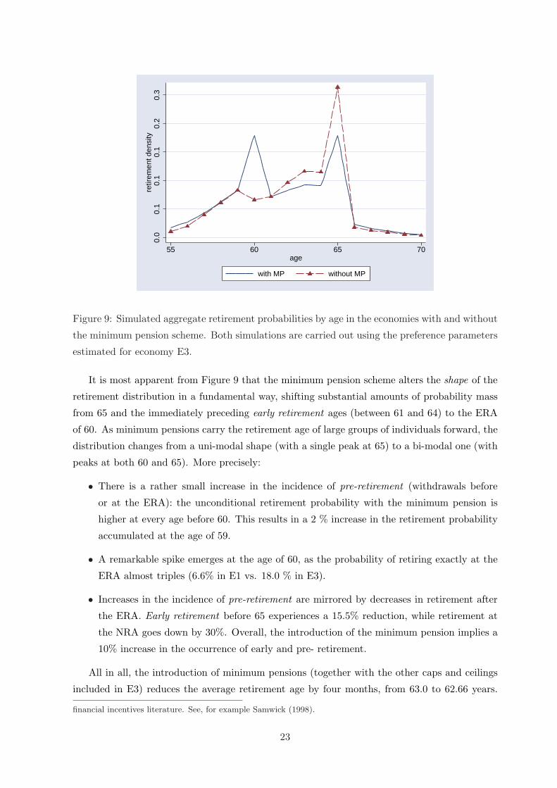
Figure 9: Simulated aggregate retirement probabilities by age in the economies with and without

the minimum pension scheme. Both simulations are carried out using the preference parameters

estimated for economy E3.

It is most apparent from Figure 9 that the minimum pension scheme alters the shape of the

retirement distribution in a fundamental way, shifting substantial amounts of probability mass

from 65 and the immediately preceding early retirement ages (between 61 and 64) to the ERA

of 60. As minimum pensions carry the retirement age of large groups of individuals forward, the

distribution changes from a uni-modal shape (with a single peak at 65) to a bi-modal one (with

peaks at both 60 and 65). More precisely:

• There is a rather small increase in the incidence of pre-retirement (withdrawals before

or at the ERA): the unconditional retirement probability with the minimum pension is

higher at every age before 60. This results in a 2 % increase in the retirement probability

accumulated at the age of 59.

• A remarkable spike emerges at the age of 60, as the probability of retiring exactly at the

ERA almost triples (6.6% in E1 vs. 18.0 % in E3).

• Increases in the incidence of pre-retirement are mirrored by decreases in retirement after

the ERA. Early retirement before 65 experiences a 15.5% reduction, while retirement at

the NRA goes down by 30%. Overall, the introduction of the minimum pension implies a

10% increase in the occurrence of early and pre- retirement.

All in all, the introduction of minimum pensions (together with the other caps and ceilings

included in E3) reduces the average retirement age by four months, from 63.0 to 62.66 years.

financial incentives literature. See, for example Samwick (1998).

23

Most changes occur at the lowest end of the income distribution, as figure 7 in the preceding

section makes clear. The retirement behavior of median and high income workers is largely

unaffected by the institutional change involved by shifting form E1 to E3.

5.1.1 Welfare impact of the minimum pension scheme

Low income workers, then, are the principal beneficiaries of the minimum pension scheme. Ar-

guably this comes at the price of higher average contributions for the overall working population,

emphasizing the distinctive redistributive character of this piece of the pension regulations.17 It

is clear that both effects should be accounted for by any measure of the average welfare impact

of minimum pensions. In this paper we assess the welfare effect by computing a compensated

equivalent variation that keeps constant the average generosity of the system (in terms of its

implicit internal rate of return). More precisely, we proceed as follows: 18

1. Evaluate the generosity of the current system by computing its average internal rate of

return r.

2. Compute the contribution rate needed to keep r constant in a system without minimum

pensions (and letting individual adjust their optimal life cycle behavior to the new insti-

tutional environment).

3. Compute the equivalent variation associated with the presence of minimum pensions, but

keeping the average generosity constant.

Proceeding in this way we find that the average welfare gain produced by minimum pensions

is not very large: it amounts to approximately 0.6% of the life-cycle consumption of the median

worker in the economy. This low figure is, of course, the result of the cancelation of effects of

opposite sign for different individuals. The gain for a low income worker that retires at the age

of 60 is a substantial 3.3% of his/her life-cycle consumption. For a worker of average earnings

that stays active till 65 the losses from higher contributions amount to almost 1% of his/her

life-cycle consumption. The detailed results can be checked in Table 6 of appendix F. Note that

these figures are extremely sensitive to changes in the growth rate of the minimum pensions.

In our benchmark simulation we assume a future growth rate of 0.5%, which is significantly

smaller than the average for the 1985/2004 interval. Had we extrapolated the historical figures,

we would have found a much larger welfare impact: an average equivalent variation of 3.6%,

and welfare gains as large as 13% of life-cycle consumption for early retirees.17In our framework, the redistributive role of minimum pensions is dominant, as the absence of health shocks

eliminate the potencial efficiency gains of early withdrawals form the labor force and unemployment benefits.18Appendix F provides formal definitions of the equivalent variation and of the compensation in generosity.

24

5.2 Early retirement and borrowing constraints

In this section we explore what arguably is the main drawback of the life cycle setting: the

very minor role played by credit restrictions. In section 5.2.1 we show that credit constraints

hardly affect optimal retirement patterns in our benchmark model (ie, when decisions are taken

early in the life-cycle by agents with a homogenous discount factor). Things may be different

in a population with heterogenous δ, as this would endogenously generate credit-constrained

individuals who may early retire in absence of minimum pensions. This possibility is explored

in section 5.2.2. We find that the quantitative bias introduced by this possibility in our main

results is small.

5.2.1 The impact of the borrowing constraint in our benchmark model

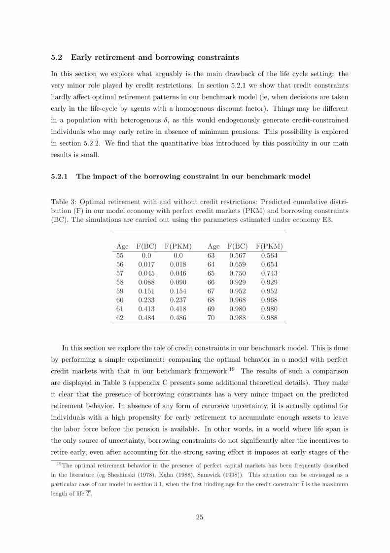
Table 3: Optimal retirement with and without credit restrictions: Predicted cumulative distri-bution (F) in our model economy with perfect credit markets (PKM) and borrowing constraints(BC). The simulations are carried out using the parameters estimated under economy E3.

Age F(BC) F(PKM) Age F(BC) F(PKM)55 0.0 0.0 63 0.567 0.56456 0.017 0.018 64 0.659 0.65457 0.045 0.046 65 0.750 0.74358 0.088 0.090 66 0.929 0.92959 0.151 0.154 67 0.952 0.95260 0.233 0.237 68 0.968 0.96861 0.413 0.418 69 0.980 0.98062 0.484 0.486 70 0.988 0.988

In this section we explore the role of credit constraints in our benchmark model. This is done

by performing a simple experiment: comparing the optimal behavior in a model with perfect

credit markets with that in our benchmark framework.19 The results of such a comparison

are displayed in Table 3 (appendix C presents some additional theoretical details). They make

it clear that the presence of borrowing constraints has a very minor impact on the predicted

retirement behavior. In absence of any form of recursive uncertainty, it is actually optimal for

individuals with a high propensity for early retirement to accumulate enough assets to leave

the labor force before the pension is available. In other words, in a world where life span is

the only source of uncertainty, borrowing constraints do not significantly alter the incentives to

retire early, even after accounting for the strong saving effort it imposes at early stages of the19The optimal retirement behavior in the presence of perfect capital markets has been frequently described

in the literature (eg Sheshinski (1978), Kahn (1988), Samwick (1998)). This situation can be envisaged as a

particular case of our model in section 3.1, when the first binding age for the credit constraint t is the maximum

length of life T .

25

life cycle. This means that the presence of recursive uncertainty (i.e. health, unemployment or

income shocks) is instrumental for making the credit constraints the key factor after the intense

retirement flows observed at the ERA (as emphasized in eg. French (2005)).

Alternatively, a life-cycle model without recursive uncertainty may produce an age-60 spike

if very impatient individuals were included in it. Those individuals optimally accumulate little

wealth along their working careers and are, consequently, strongly credit constrained in the years

immediately before ERA. In these circumstances, they have no real option to retire until the

public pension is first available. Furthermore, very impatient individuals are not much affected

by the strong forces retaining workers at that particular age (stemming basically from increases

in the future pension, recall section 3.2), as they discount these future gains strongly.20 These

two observations together suggest that these workers may find it optimal to retire at 60 even in

absence of minimum pensions. This possibility is quantitatively evaluated in the next section.

5.2.2 Early retirement with heterogeneity in the discount factor

54 56 58 60 62 64 66 680

0.2

0.4

0.6

0.8

1

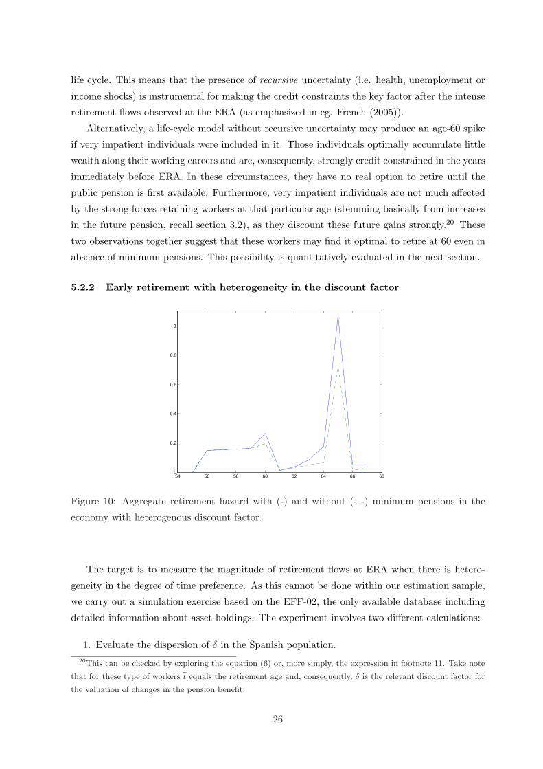
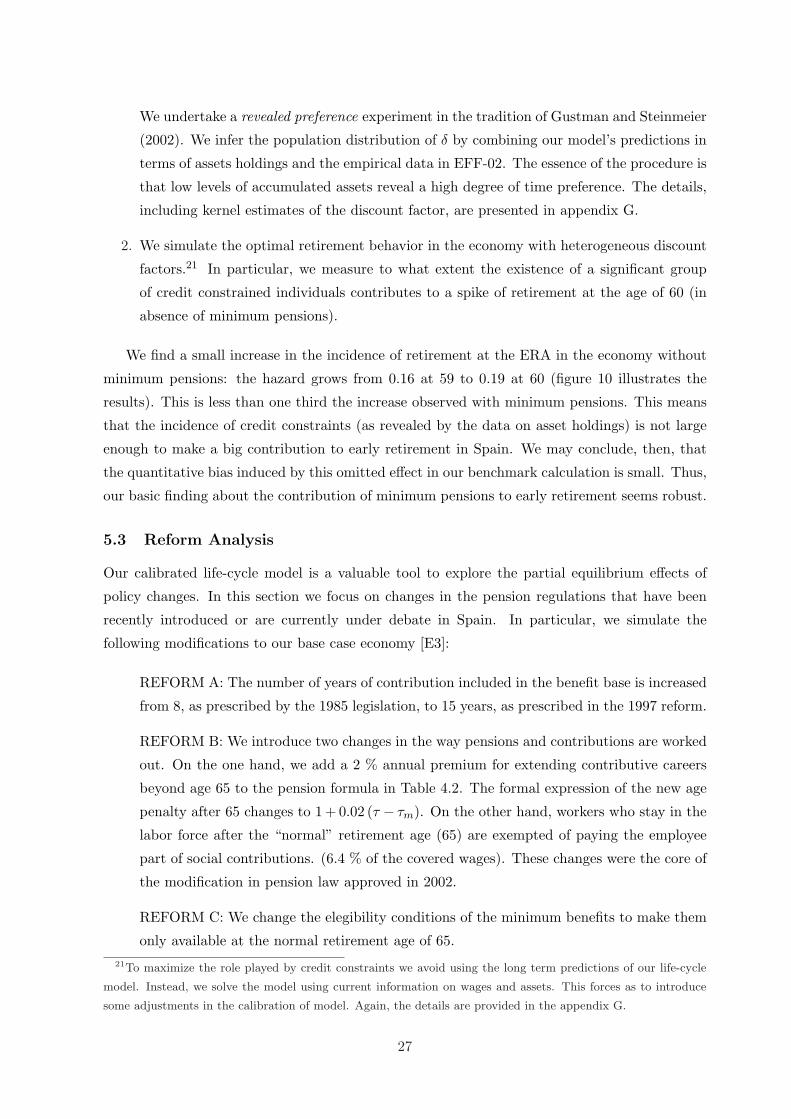
Figure 10: Aggregate retirement hazard with (-) and without (- -) minimum pensions in the

economy with heterogenous discount factor.

The target is to measure the magnitude of retirement flows at ERA when there is hetero-

geneity in the degree of time preference. As this cannot be done within our estimation sample,

we carry out a simulation exercise based on the EFF-02, the only available database including

detailed information about asset holdings. The experiment involves two different calculations:

1. Evaluate the dispersion of δ in the Spanish population.20This can be checked by exploring the equation (6) or, more simply, the expression in footnote 11. Take note

that for these type of workers t equals the retirement age and, consequently, δ is the relevant discount factor for

the valuation of changes in the pension benefit.

26

We undertake a revealed preference experiment in the tradition of Gustman and Steinmeier

(2002). We infer the population distribution of δ by combining our model’s predictions in

terms of assets holdings and the empirical data in EFF-02. The essence of the procedure is

that low levels of accumulated assets reveal a high degree of time preference. The details,

including kernel estimates of the discount factor, are presented in appendix G.

2. We simulate the optimal retirement behavior in the economy with heterogeneous discount

factors.21 In particular, we measure to what extent the existence of a significant group

of credit constrained individuals contributes to a spike of retirement at the age of 60 (in

absence of minimum pensions).

We find a small increase in the incidence of retirement at the ERA in the economy without

minimum pensions: the hazard grows from 0.16 at 59 to 0.19 at 60 (figure 10 illustrates the

results). This is less than one third the increase observed with minimum pensions. This means

that the incidence of credit constraints (as revealed by the data on asset holdings) is not large

enough to make a big contribution to early retirement in Spain. We may conclude, then, that

the quantitative bias induced by this omitted effect in our benchmark calculation is small. Thus,

our basic finding about the contribution of minimum pensions to early retirement seems robust.

5.3 Reform Analysis

Our calibrated life-cycle model is a valuable tool to explore the partial equilibrium effects of

policy changes. In this section we focus on changes in the pension regulations that have been

recently introduced or are currently under debate in Spain. In particular, we simulate the

following modifications to our base case economy [E3]:

REFORM A: The number of years of contribution included in the benefit base is increased

from 8, as prescribed by the 1985 legislation, to 15 years, as prescribed in the 1997 reform.

REFORM B: We introduce two changes in the way pensions and contributions are worked

out. On the one hand, we add a 2 % annual premium for extending contributive careers

beyond age 65 to the pension formula in Table 4.2. The formal expression of the new age

penalty after 65 changes to 1 + 0.02 (τ − τm). On the other hand, workers who stay in the

labor force after the “normal” retirement age (65) are exempted of paying the employee

part of social contributions. (6.4 % of the covered wages). These changes were the core of

the modification in pension law approved in 2002.

REFORM C: We change the elegibility conditions of the minimum benefits to make them

only available at the normal retirement age of 65.21To maximize the role played by credit constraints we avoid using the long term predictions of our life-cycle

model. Instead, we solve the model using current information on wages and assets. This forces as to introduce

some adjustments in the calibration of model. Again, the details are provided in the appendix G.

27

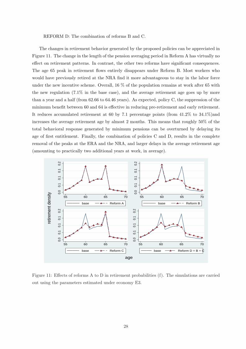
REFORM D: The combination of reforms B and C.

The changes in retirement behavior generated by the proposed policies can be appreciated in

Figure 11. The change in the length of the pension averaging period in Reform A has virtually no

effect on retirement patterns. In contrast, the other two reforms have significant consequences.

The age 65 peak in retirement flows entirely disappears under Reform B. Most workers who

would have previously retired at the NRA find it more advantageous to stay in the labor force

under the new incentive scheme. Overall, 16 % of the population remains at work after 65 with

the new regulation (7.1% in the base case), and the average retirement age goes up by more

than a year and a half (from 62.66 to 64.46 years). As expected, policy C, the suppression of the

minimum benefit between 60 and 64 is effective in reducing pre-retirement and early retirement.

It reduces accumulated retirement at 60 by 7.1 percentage points (from 41.2% to 34.1%)and

increases the average retirement age by almost 2 months. This means that roughly 50% of the

total behavioral response generated by minimum pensions can be overturned by delaying its

age of first entitlement. Finally, the combination of policies C and D, results in the complete

removal of the peaks at the ERA and the NRA, and larger delays in the average retirement age

(amounting to practically two additional years at work, in average).

0.0

0.1

0.1

0.1

0.2

55 60 65 70

base Reform A

0.0

0.1

0.1

0.1

0.2

55 60 65 70

base Reform B

0.0

0.1

0.1

0.1

0.2

55 60 65 70

base Reform C

0.0

0.1

0.1

0.1

0.2

55 60 65 70

base Reform D = B + C

retir

emen

t den

sity

age

Figure 11: Effects of reforms A to D in retirement probabilities (f). The simulations are carried

out using the parameters estimated under economy E3.

28

6 Conclusions

The minimum pension scheme is one of the largest programs of the Spanish Old Age pension

system. It provides substantial income support for a large number of Spanish pensioners, which

has gained it widespread popularity. The efficiency properties of this mechanism, however, have

received little attention so far. In this paper we both quantify the welfare impact of minimum

pensions and study the magnitude of the distortions generated by this piece of regulation on

retirement behavior. We undertake this analysis with the help of a stylized life cycle model,

which allows for a very convenient analytical characterization of the optimality conditions, and

which can be solved with much less computational effort than what is needed with a standard

Dynamic Programming model. We use this model as the data generating process in a structural

estimation experiment, finding that our stylized model provides a rather good approximation of

empirical retirement behavior, using a minimum amount of information.

Once these maximum likelihood estimations are fed into the model, we are left with a fully

operative tool for policy analysis. Our main experiment is a quantitative evaluation of the

impact of the minimum pension on early retirement. We find that the incidence of retirement

at the age of first entitlement (60) almost triples with respect to that in the economy without

minimum pensions, and total early retirement (before or at 60) is almost 50% larger with

minimum pensions. We check that these findings are robust to the inclusion of heterogeneity

in the discount factor (ie, in situation where the role of credit constraints is much reinforced).

We also explore the impact of several policy changes already implemented or currently under

debate in Spain.

Our findings make it clear that minimum pensions should receive more attention in the cur-

rent debate about the reform of the pension system in Spain (or any country with a similar

system). It is clearly a contradiction to discuss changes aimed at fostering older workers’ labor

participation and, at the same time, to ignore the strong disincentive effects of minimum pen-

sions. We conclude with a few remarks about some drawbacks of the current experiment and

some future lines of research. Firstly, the magnitude of the behavioral changes induced by the

minimum pensions is high enough for general equilibrium effects to be sizeable. An evaluation

of the quantitative importance of these effects would be desirable (see Sanchez-Martın (2002))

for a first evaluation in an OLG context). A second aspect of our model that demands a serious

reconsideration is the absence of any form of recursive uncertainty. Health and unemployment

shocks are particularly well worth considering, as they can have a strong influence on retirement

decisions in economies with imperfect insurance. Extending the life-cycle model to include these

features is a promising, although quite demanding, research effort for the immediate future.

29

REFERENCES

Boldrin M, Jimenez-Martın M, Peracchi F. 1999. Social security and retirement in Spain. In Social

Security and Retirement around the world, Jonathan Gruber and David Wise (eds). University of

Chicago Press for the NBER: Chicago.

Boldrin M, Jimenez-Martın M, Peracchi F. 2004. Micromodeling of social security and retirement

in Spain. In Social Security and Retirement around the world: micro-estimation, Jonathan Gruber

and David Wise (eds). University of Chicago Press for the NBER: Chicago.

Crawford VP, Lilien DM. 1981. Social security and the retirement decision. Quarterly Journal of

Economics 96: 505-529.

Fabel O. 1994a. The economics of Pensions and Variable Retirement Schemes. Series in Financial

Economics and Quantitative Analysis. John Wiley & Sons.

Fabel 0. 1994b. Social security, optimal retirement and savings. European Journal of Political

Economy 10: 783-802.

French E. 2005. The effects of health, wealth, and wages on labor supply and retirement behavior.

Review of Economic Studies 72: 395-427.

French E, Jones JB. 2001. The effects of health insurance and self-insurance on retirement be-

haviour.Working paper series, Research Department, wp 2001-19, Federal Reserve Bank of Chicago.

Gruber J, Wise D (eds). 1999. Social Security and Retirement around the World. University of

Chicago Press: Chicago.

Gustman A, Steinmeier T. 1986. A structural retirement model. Econometrica 54: 555-584.

Gustman A, Steinmeier T. 2002. The social security early retirement age in a structural model of

retirement and wealth. Working paper n. 9183, National Bureau of Economic Research.

Hurd MD. 1989. Mortality risk and bequest. Econometrica 57: 779-813.

Jimenez-Martın S, Sanchez-Martın AR. 2003. An evaluation of the life-cycle effects of minimum

pensions on retirement behavior. Working Paper 715, Universitat Pompeu Fabra.

Jimenez-Martın S, Sanchez-Martın AR. 2004. The effects of pension rules on monetary incentives

to retirement, with an application to the analysis of pension reform in Spain. Hacienda Publica

Espanola 169: 35-66.

Kahn JA. 1988. Social security, liquidity and early retirement. Journal of Public Economics 89:

97-117.

Kalisch DW, Aman T. 1998. Retirement income systems: The reform process across OECD

countries. AWP3.4. OECD: Paris.

Leung SF. 1994. Uncertain lifetime, the theory of the consumer, and the life cycle hypothesis.

Econometrica 62: 1233-1239.

Leung SF. 2000. Why do some households save so little? a rational explanation. Review of

Economic Dynamics 3: 771-800.

30

Lumsdaine RL, Stock JH, Wise DA. 1992. Three models of retirement: computational complexity

versus predictive validity. In Topics in the economics of aging. Wise DA (ed). Chicago University

Press for the NBER: Chicago.

Modigliani F, Brumberg R. 1980. Utility analysis and aggregate consumption functions: an attempt

at integration. In The Collected Papers of Franco Modigliani. Abel A (ed). MIT: Cambridge, MA.

Rust J, Phelan C. 1997. How social security and medicare affect retirement behavior in a world of

incomplete markets. Econometrica 65: 781-831.

Samwick A. 1998. New evidence on pensions, social security and the timing of retirement. Journal

of Public Economics 70: 207-236.

Sanchez-Martın AR. 2002. Endogenous retirement and public pension system reform in Spain.

Mimeo.

Sheshinski E. 1978. A model of social security and retirement decisions. Journal of Public Eco-

nomics 10: 337-360.

Yaari ME. 1965. Uncertain lifetime, life insurance and the theory of the consumer. Review of

Economic Studies 32: 137-150.

31

APPENDIX

A The solution of the individual problem

In section 3 we show how the original constrained problem in (1) is transformed into the un-

constrained one in (2). This new problem is dealt with in three stages. In the next section we

review how to analytically characterize the optimal profiles of consumption and accumulated

assets for a given retirement age and a given binding age for the credit constraint. In section

A.2 we show how to use these conditional solutions to compute the optimal binding age for any

given retirement age.

A.1 The conditional consumption/savings problem

When both the retirement, τ , and the wealth depletion age, t, are fixed, a straightforward

application of Optimal Control Theory allows for a complete characterization of the optimal

conditional consumption function cτ (. |t) (ie, the solution to problem (2)). 22 Omitting the

dependence on τ and t to make notation easier, the Hamiltonian of the system is:

H(a(t), c(t), λ(t), t, τ) = e−δ(t) [ u(c(t)) + ν(lτ (t)) ] + λ(t) (r a(t) + w(t)− c(t))

Denoting a solution by x = {a, c, λ}, it must satisfy the following first order conditions, ∀t ∈[t0, t]:

∂ H(x(t), t, τ)∂ c(t)

≡ e−δ t d u

dc(c(t))− λ(t) = 0 (12)

∂ H(x(t), t, τ)∂ a(t)

≡ r λ(t) = −λ(t) (13)

a(t) = r a(t) + w(t)− c(t) (14)

a(t0) = a0 ; a(t) = 0 (15)

It is easy to check that these conditions are also sufficient for our problem. To get to expression

(17) we proceed as follows:

1. We integrate (13) to obtain λ(t) as a function of λ(t0) (just λ in our notation). If this is

particularized in (12), we obtain:

e−δ(t) d u

dc(c(t)) = λ e−r t (16)

2. If we integrate (14) we obtain the conditional Intertemporal Budget constraint (IBC).22Our problem differs from the standard formulation (as stated in eg. ?), pag 165, or ?), pag 84) due to the

existence of a couple of discontinuities in the retirement age. The first one appears in the objective function, as

a result of the leisure component; while the second one shows up in the system’s dynamic equation, stemming

from the pension rules. The optimality conditions are, however, standard as all the relevant regularity conditions

apply to our problem (see note 6 in ?), pag 87).

32

3. If we further restrict ourselves to the CES case, u(c) = c1−η/(1 − η), we can express

the optimal conditional consumption c(t) as an explicit function of λ from (16). This,

in turn, can be particularized in the conditional IBC. Obtaining the optimal conditional

consumption is then straightforward:

cτ (t | t) =[S(t)d(t)]γ

Cc(t)Y (τ, t) with Cc(t) =

∫ t

t0e−r (t−t0) [S(t) d(t)]γ dt (17)

where γ stands for the intertemporal elasticity of substitution γ = 1/η, d(t) = e(r−δ) (t−t0)

is the net discounted factor, Cc(t) is an integrating constant (ensuring that the present

discounted values of earnings and consumption are equal), and Y (τ, t) is the Conditional

Life-cycle Wealth:

Y (τ, t) = a0 +∫ τ

t0e−r (t−t0) w(t)(1− ς) dt +

∫ t

τe−r (t−t0) b(t, τ) dt (18)

Expressions (17) and (18) make it easy to study the dependence of optimal consumption on

individual preferences, life cycle income and the survival profile, given a specific institutional

environment. They also allow the optimal conditional consumption profile to be calculated very

quickly.

As the survival probability eventually goes to zero as age increases, the optimal conditional

consumption profile must be eventually decreasing. Intuitively, there must be an age t∗ where

the constant or increasing pension benefits equal the decreasing conditional consumption, i.e.

cτ (t∗ |t) = b(τ). Assume we represent this relation via the function hτ (t). Of course, there is no

guarantee that t∗ ≡ hτ (t) = t for an arbitrary wealth depletion age t. As we show in the next

paragraph, this condition defines the “optimal” binding age for the credit constraint. Therefore,

finding the right unconditional optimal consumption function (for every retirement age) requires

finding the unique fix point of hτ (.).

A.2 The Optimal binding age for the credit constrain

If we particularize the previous optimal conditional consumption function cτ (t | t) in problem

(2) objective function, we are left with the following “concentrated” problem, which provides

the optimal wealth depletion age for a given retirement age:

max V (t) =∫ tt0

e−δ(t)u( cτ (t | t) ) dt +∫ Tt e−δ(t)u(b(t, τ)) dt

t ∈ [τ , T ]

Given τ, cτ (t | t) : [t0, t] →R+ and τ = max{τm, τ}(19)

Under our assumptions, the solution to this problem coincides with the intuitive proposal

we stated at the end of the previous section: the optimal t is implicitly defined as a fixed point

of the function hτ (.)

t∗ ≡ hτ (t) = t (20)

33

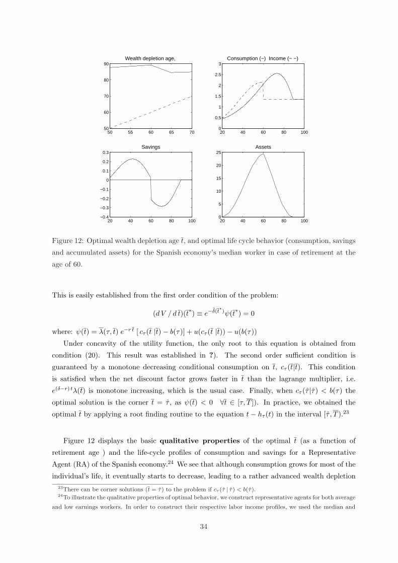
50 55 60 65 7050

60

70

80

90Wealth depletion age,

20 40 60 80 1000

0.5

1

1.5

2

2.5

3Consumption (−) Income (− −)

20 40 60 80 100−0.4

−0.3

−0.2

−0.1

0

0.1

0.2

0.3Savings

20 40 60 80 1000

5

10

15

20

25Assets

Figure 12: Optimal wealth depletion age t, and optimal life cycle behavior (consumption, savings

and accumulated assets) for the Spanish economy’s median worker in case of retirement at the

age of 60.

This is easily established from the first order condition of the problem:

(d V / d t)(t∗) ≡ e−δ(t∗)ψ(t∗) = 0

where: ψ(t) = λ(τ, t) e−r t [ cτ (t |t)− b(τ)] + u(cτ (t |t))− u(b(τ))

Under concavity of the utility function, the only root to this equation is obtained from

condition (20). This result was established in ?). The second order sufficient condition is

guaranteed by a monotone decreasing conditional consumption on t, cτ (t|t). This condition

is satisfied when the net discount factor grows faster in t than the lagrange multiplier, i.e.

e(δ−r) tλ(t) is monotone increasing, which is the usual case. Finally, when cτ (τ |τ) < b(τ) the

optimal solution is the corner t = τ , as ψ(t) < 0 ∀t ∈ [τ, T ]). In practice, we obtained the

optimal t by applying a root finding routine to the equation t− hτ (t) in the interval [τ , T ).23

Figure 12 displays the basic qualitative properties of the optimal t (as a function of

retirement age ) and the life-cycle profiles of consumption and savings for a Representative

Agent (RA) of the Spanish economy.24 We see that although consumption grows for most of the

individual’s life, it eventually starts to decrease, leading to a rather advanced wealth depletion23There can be corner solutions (t = τ) to the problem if cτ (τ | τ) < b(τ).24To illustrate the qualitative properties of optimal behavior, we construct representative agents for both average

and low earnings workers. In order to construct their respective labor income profiles, we used the median and

34

age. Therefore, the credit constraint becomes binding only for the very elderly. Median workers

accumulate assets right after the entrance into the labor market, and start depleting assets only

after retirement.

B General expressions for the marginal utility of working

The general procedure to obtain the analytical expression for the marginal utility of working at

any age τ is as follows:

1. Differentiate the expression of E[V ] in (1) with respect to both τ and consumption.

2. Particularize the first order condition of the optimal consumption problem (16) and group

all terms containing d cτ/d τ .

3. Differentiate the conditional intertemporal budget constraint with respect to τ and gather

all the terms containing d cτ/d τ .

4. Particularize the expression in step 3 into the general equation obtained in step 2. In this

way we disposed of the term containing the consumption derivative, and we are left with

a general analytical expression for optimal retirement.

The general expression (omitting the leisure component) when there are no minimum pen-

sions is:

d Vd τ (τ) = λ(τ, t) d(τ) [w(τ)(1− ς)− I(τ = τ) I(τ < t) b + b′A(τ , t)+

e−r (t−τ)( I(τ < t) b− c(t) ) d td τ ]+

eδ(τ)−δ(t) ( u(c)− u(b)) d td τ + b′ u′(b)Aδ(t, T )

where t = t(τ), b = b(τ); b′ = b′(τ), c(.) = cτ (.|t), d(t) = e(r−δ) (t−t0), A(τ , t) =∫ tτ e−r t dt and

Aδ(t, T ) =∫ Tt e−δ(t) dt. When the pension system includes a guarantee minimum the expression

becomes a bit more complicated:

d Vd τ (τ) = λ(τ, t, J) d(τ) [ w(τ)(1− ς)− I(τ = τ) I(τ < t) b + b′A(τ , t)+

e−r (t−τ)( I(τ < t) b− c(t) ) d td τ ]+

eδ(τ)−δ(J) ( I(t < J) u(b)− I(J < T ) u(bmJ) d Jd τ +

eδ(τ)−δ(t) ( u(c)− I(t < J)u(b)) d td τ +

b′ u′(b)Aδ(t, J)

where J = J(τ) is the age when the minimum pension becomes binding.

the 10th percentile of the empirical distribution in 1994 wave from the European Community Household Panel

(ECHP). The survival probabilities and all the other environmental parameters are identical to those used in

the estimation of the model (see section 4.2). The preference parameters employed are our maximum likelihood

estimations in section 4.

35

50 52 54 56 58 60 62 64 66 68 70−10

−8

−6

−4

−2

0

2

4

6

8

10

PKM

BC

Figure 13: Marginal utility of working with (-) and without (- -) credit constraint. Representative

(median) agent.

50 52 54 56 58 60 62 64 66 68 70−10

−8

−6

−4

−2

0

2

4

6

BC

PKM

Figure 14: Marginal utility of working with (-) and without (- -) credit constraint. Agent in the

10% quantile of the income distribution.

36

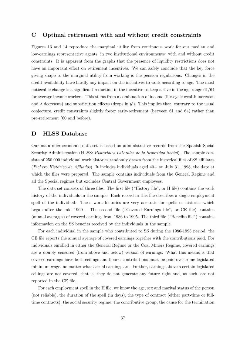
C Optimal retirement with and without credit constraints

Figures 13 and 14 reproduce the marginal utility from continuous work for our median and

low-earnings representative agents, in two institutional environments: with and without credit

constraints. It is apparent from the graphs that the presence of liquidity restrictions does not

have an important effect on retirement incentives. We can safely conclude that the key force

giving shape to the marginal utility from working is the pension regulations. Changes in the

credit availability have hardly any impact on the incentives to work according to age. The most

noticeable change is a significant reduction in the incentive to keep active in the age range 61/64

for average income workers. This stems from a combination of income (life-cycle wealth increases

and λ decreases) and substitution effects (drops in y′). This implies that, contrary to the usual

conjecture, credit constraints slightly foster early-retirement (between 61 and 64) rather than

pre-retirement (60 and before).

D HLSS Database

Our main microeconomic data set is based on administrative records from the Spanish Social

Security Administration (HLSS: Historiales Laborales de la Seguridad Social). The sample con-

sists of 250,000 individual work histories randomly drawn from the historical files of SS affiliates

(Fichero Historico de Afiliados). It includes individuals aged 40+ on July 31, 1998, the date at

which the files were prepared. The sample contains individuals from the General Regime and

all the Special regimes but excludes Central Government employees.

The data set consists of three files. The first file (“History file”, or H file) contains the work

history of the individuals in the sample. Each record in this file describes a single employment

spell of the individual. These work histories are very accurate for spells or histories which

began after the mid–1960s. The second file (“Covered Earnings file”, or CE file) contains

(annual averages) of covered earnings from 1986 to 1995. The third file (“Benefits file”) contains

information on the SS benefits received by the individuals in the sample.

For each individual in the sample who contributed to SS during the 1986-1995 period, the

CE file reports the annual average of covered earnings together with the contributions paid. For

individuals enrolled in either the General Regime or the Coal Miners Regime, covered earnings

are a doubly censored (from above and below) version of earnings. What this means is that

covered earnings have both ceilings and floors: contributions must be paid over some legislated

minimum wage, no matter what actual earnings are. Further, earnings above a certain legislated

ceilings are not covered, that is, they do not generate any future right and, as such, are not

reported in the CE file.

For each employment spell in the H file, we know the age, sex and marital status of the person

(not reliable), the duration of the spell (in days), the type of contract (either part-time or full-

time contracts), the social security regime, the contributive group, the cause for the termination

37

of the spell, the sector of employment (4-digits SIC), and the region of residence (52 Spanish

provinces). We restrict our empirical analysis to the sample of male workers enroled in the

General Regime in 1995, that have been working continuously from 1986 to 1994. Descriptive

statistics of the variables employed are presented in table D. We refer to Boldrin et al. (2004)

for a more detailed description of the variables in the HLSS files.

Table 4: Descriptive statisticsby education Total Edu high Edu low

# observations: 16359 1472 14887mean s.e. mean s.e. mean s.e.

%retiring .122 .328 .0822 .274 .1268 .332High education .0899 .286 — — — —Age 58.90 2.96 59.28 3.33 58.86 2.92Receipt temporary benefits .3272 .469 .1637 .370 .343 .474Years of contribution 31.4 5.72 31.76 5.53 31.44 5.73Wagea 2.420 1.56 4.502 2.25 2.215 1.31Benefit basea 2.17 1.02 3.553 1.17 2.030 .897Theoretical Benefita 1.33 .728 2.246 .947 1.244 .635Effective benefita .627 .930 1.17 1.49 .5730 .835

by age group 55–59 60–64 65+# observations: 9970 5716 673

mean s.e. mean s.e. mean s.e.%retiring .0342 .181 .206 .405 .7221 .448High education .0818 .270 .0970 .296 .1500 .357Age 56.91 1.48 61.58 1.39 65.53 1.16Receipt temporary benefits .3118 .463 .3497 .476 .3655 .481Years of contribution 29.85 5.25 33.90 5.40 34.69 6.27Wagea 2.471 1.61 2.362 1.47 2.165 1.50Benefit basea 2.169 1.03 2.192 .995 2.092 1.11Theoretical Benefita 1.178 .601 1.528 .770 2.007 1.12Effective benefita — — 1.558 .741 2.018 1.11a: (in 106 1995 pta)

Earnings distribution, earnings histories and projections

As commented in the previous section, we do not observe earnings directly but only covered

earnings (i.e. a doubly censored version of earnings). To deal with the top-censoring problem,

we proceed as follows. First we estimate a Tobit model for (log) covered earnings. Then we use

the estimated parameters to impute the earnings of the censored observations and estimate an

earning function using imputed earnings for those affected by the ceilings. Finally, we gener-

ate “true earnings” for all the individuals in the top censored groups, by using the estimated

regression function and adding an individual random noise component.

From the individual profile of covered earnings ct between year 1986 and year 1995 = T

we impute the individual profile of “true” real earnings (wt, t = 1986, . . . , 1995). Given this

information, we “smoothly” project earnings forward and backward in the following way:

wT+k = wT + g(aT+k) for k = −KL, . . . , 0, . . . , +KH

38

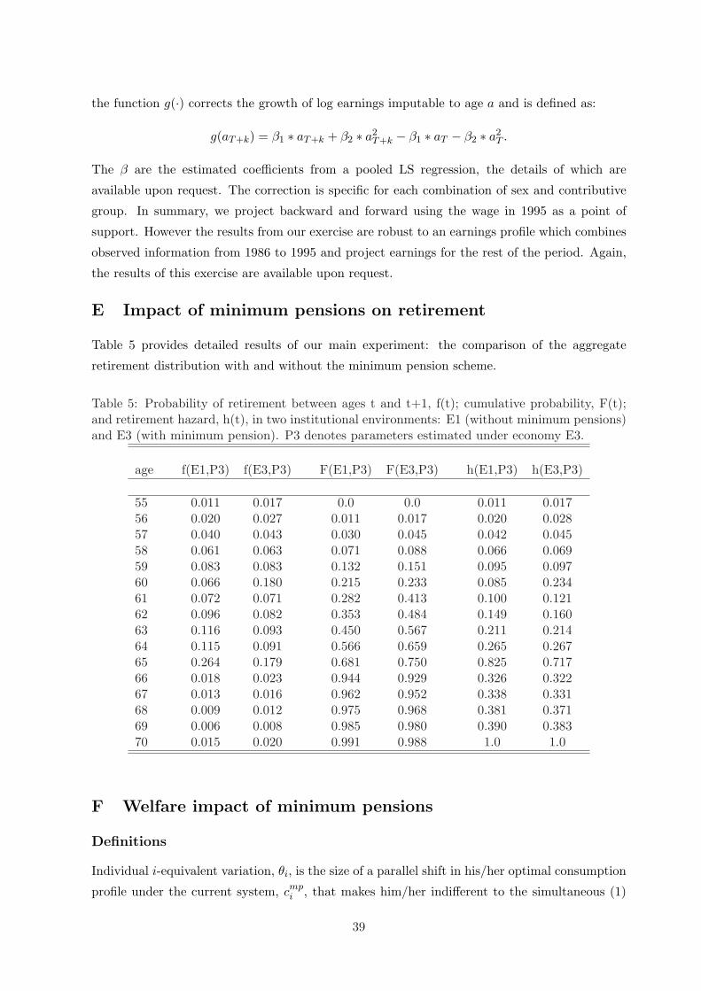
the function g(·) corrects the growth of log earnings imputable to age a and is defined as:

g(aT+k) = β1 ∗ aT+k + β2 ∗ a2T+k − β1 ∗ aT − β2 ∗ a2

T .

The β are the estimated coefficients from a pooled LS regression, the details of which are

available upon request. The correction is specific for each combination of sex and contributive

group. In summary, we project backward and forward using the wage in 1995 as a point of

support. However the results from our exercise are robust to an earnings profile which combines

observed information from 1986 to 1995 and project earnings for the rest of the period. Again,

the results of this exercise are available upon request.

E Impact of minimum pensions on retirement

Table 5 provides detailed results of our main experiment: the comparison of the aggregate

retirement distribution with and without the minimum pension scheme.

Table 5: Probability of retirement between ages t and t+1, f(t); cumulative probability, F(t);and retirement hazard, h(t), in two institutional environments: E1 (without minimum pensions)and E3 (with minimum pension). P3 denotes parameters estimated under economy E3.

age f(E1,P3) f(E3,P3) F(E1,P3) F(E3,P3) h(E1,P3) h(E3,P3)

55 0.011 0.017 0.0 0.0 0.011 0.01756 0.020 0.027 0.011 0.017 0.020 0.02857 0.040 0.043 0.030 0.045 0.042 0.04558 0.061 0.063 0.071 0.088 0.066 0.06959 0.083 0.083 0.132 0.151 0.095 0.09760 0.066 0.180 0.215 0.233 0.085 0.23461 0.072 0.071 0.282 0.413 0.100 0.12162 0.096 0.082 0.353 0.484 0.149 0.16063 0.116 0.093 0.450 0.567 0.211 0.21464 0.115 0.091 0.566 0.659 0.265 0.26765 0.264 0.179 0.681 0.750 0.825 0.71766 0.018 0.023 0.944 0.929 0.326 0.32267 0.013 0.016 0.962 0.952 0.338 0.33168 0.009 0.012 0.975 0.968 0.381 0.37169 0.006 0.008 0.985 0.980 0.390 0.38370 0.015 0.020 0.991 0.988 1.0 1.0

F Welfare impact of minimum pensions

Definitions

Individual i-equivalent variation, θi, is the size of a parallel shift in his/her optimal consumption

profile under the current system, cmpi , that makes him/her indifferent to the simultaneous (1)

39

elimination of the minimum pension and (2) reduction in the contribution rate that keeps the

average generosity constant. Formally:

V mpi (cmp

i (1 + θi), τmpi | ςmp) = V ∗

i (c∗i , τ∗i | ς∗)

where V ji , cj

i , τji and ςj stand for life-cycle utility, consumption, optimal retirement and con-

tribution rate under system j. The current system (j = mp) includes real-world contribution

rates and minimum pensions. In the alternative system j = ∗ minimum pensions are absent and

contributions are reduced to ς∗ (a rate that guarantees the same average generosity in absence of

minimum pensions. We measure the average generosity under system j by the average internal

rate of return: rj =∫i r(i)

j dP (i), with P (i) denoting agent i measure. The r(i) are defined in a

standard way (the rates that match the expected discounted value of life cycle pension benefits

and contributions).

Detailed calculations

The welfare calculation involves three steps:

1. To compute the current system’s average internal rate of return r we partition the sample

(active individuals aged 55 or older) according to the wage and educational levels. Each

individual is then assigned a “type” i of the I possible observable groups. The empirical

measure (weight) of each group is denoted µi. Recall than, on top of this observable

heterogeneity, individuals differ in their unobservable relative value of leisure (implying

different consumption paths and retirement ages for otherwise identical households). rmp

is then computed as follows:

(a) We calculate rmpi (τ) ∀i ∈ I and for each possible retirement age. This implies solving

the following nonlinear equation:

τ−1∑

a=20

Sacotia

(1 + rmpi (τ))a

=T∑

a=τ

Sabia(τ)

(1 + rmpi (τ))a

where cotia stands for age-a contributions, bia(τ) for pension income in case of retire-

ment at τ and Sa is the probability of surviving to age a (conditional on surviving

till age-20).

(b) For each i ∈ I, we compute the retirement probabilities predicted at every age by our

theoretical model, Pi(τ).

We use them to find an internal rate of return that accounts for both observable and

unobservable heterogeneity:

rmp =I∑

i=1

µi

70∑

τ=56

Pi(τ) rmpi (τ)

40

2. We work out the contribution rate (ς∗) that results in the same implicit average rate of

return in absence of minimum pensions. We allow individuals to change their optimal

consumption and retirement behavior during the process.

3. Finally, we compute the Equivalent Variation (θ) associated with the elimination of the

minimum pension scheme, while keeping constant the average generosity of the pension

system.

Table 6 presents the results obtained assuming the same parameter values implemented in

the paper.25 Table 7 shows that the results are very sensitive to the projected growth rate of the

minimum pensions. If their historical growth rates (roughly in line with average wages) were to

stay unchanged, their welfare impact would be much larger.

age High Education Average EducationQ 1/3 Q 2/3 Q 3/3 Q1/3 Q 2/3 Q 3/3

57.0000 2.5831 -0.1015 -0.1015 3.4899 -0.1017 -0.101758.0000 2.5387 -0.1021 -0.1021 3.4280 -0.1024 -0.102459.0000 2.4966 -0.1027 -0.1027 3.3692 -0.1030 -0.103060.0000 2.4568 -0.1032 -0.1032 3.3133 -0.1035 -0.103561.0000 -0.1016 -0.1016 -0.1016 -0.0923 -0.1020 -0.102062.0000 -0.1009 -0.1009 -0.1009 -0.1013 -0.1013 -0.101363.0000 -0.0999 -0.0999 -0.0999 -0.1003 -0.1003 -0.100364.0000 -0.0997 -0.0997 -0.0997 -0.1001 -0.1001 -0.100165.0000 -0.0990 -0.0990 -0.0990 -0.0995 -0.0995 -0.0995

Table 6: Compensated equivalent variation by age of retirement, education and wage level(positive signs indicates welfare gains)

age High Education Average EducationQ 1/3 Q 2/3 Q 3/3 Q1/3 Q 2/3 Q 3/3

58.0000 13.5220 -0.2308 -0.2308 13.9952 -0.2314 -0.231459.0000 13.4186 -0.2321 -0.2321 13.7802 -0.2328 -0.232860.0000 13.2362 -0.2334 -0.2334 13.6807 -0.2341 -0.234161.0000 7.7155 -0.2298 -0.2298 8.8084 -0.2306 -0.230662.0000 3.3081 -0.2281 -0.2281 4.1861 -0.2289 -0.228963.0000 0.2378 -0.2258 -0.2258 0.9270 -0.2267 -0.226764.0000 -0.2222 -0.2254 -0.2254 -0.2142 -0.2263 -0.226365.0000 -0.2239 -0.2239 -0.2239 -0.2249 -0.2249 -0.2249

Table 7: Compensated equivalent variation projecting historical growth rates of minimum pen-sions

25We consider 2 educational types and 3 labor earnings-quantiles.

41

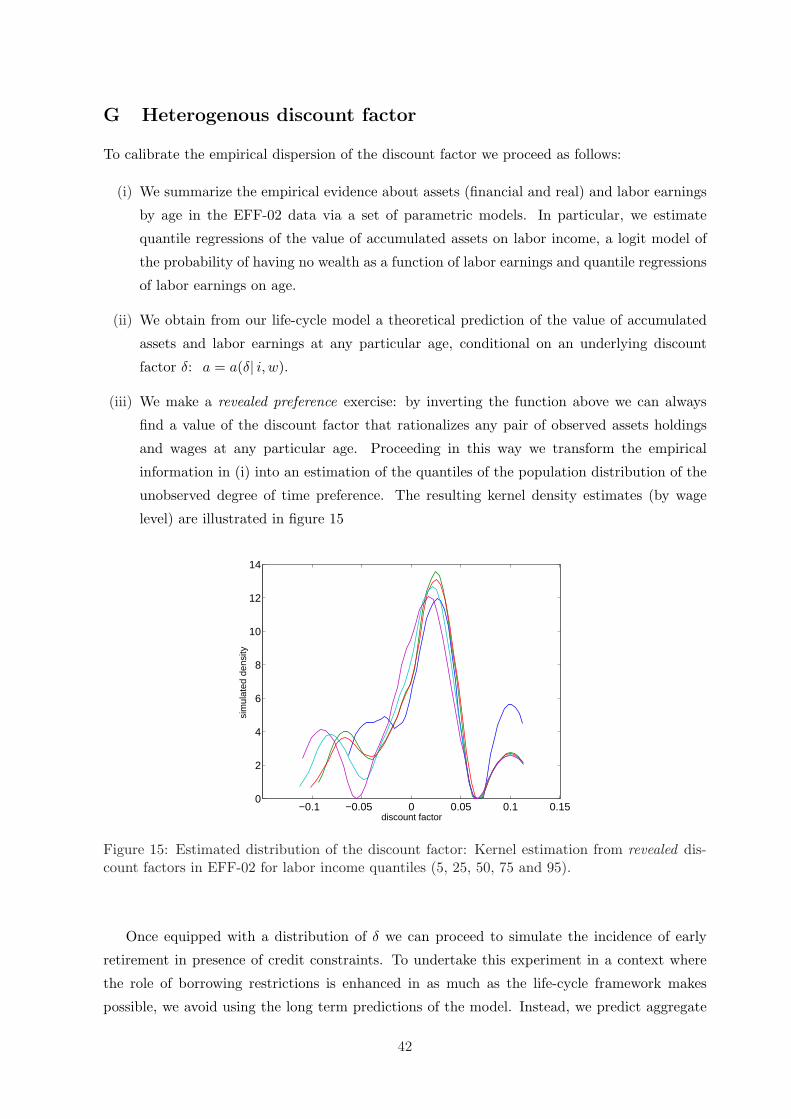
G Heterogenous discount factor

To calibrate the empirical dispersion of the discount factor we proceed as follows:

(i) We summarize the empirical evidence about assets (financial and real) and labor earnings

by age in the EFF-02 data via a set of parametric models. In particular, we estimate

quantile regressions of the value of accumulated assets on labor income, a logit model of

the probability of having no wealth as a function of labor earnings and quantile regressions

of labor earnings on age.

(ii) We obtain from our life-cycle model a theoretical prediction of the value of accumulated

assets and labor earnings at any particular age, conditional on an underlying discount

factor δ: a = a(δ| i, w).

(iii) We make a revealed preference exercise: by inverting the function above we can always

find a value of the discount factor that rationalizes any pair of observed assets holdings

and wages at any particular age. Proceeding in this way we transform the empirical

information in (i) into an estimation of the quantiles of the population distribution of the

unobserved degree of time preference. The resulting kernel density estimates (by wage

level) are illustrated in figure 15

−0.1 −0.05 0 0.05 0.1 0.150

2

4

6

8

10

12

14

discount factor

sim

ulat

ed d

ensi

ty

Figure 15: Estimated distribution of the discount factor: Kernel estimation from revealed dis-count factors in EFF-02 for labor income quantiles (5, 25, 50, 75 and 95).

Once equipped with a distribution of δ we can proceed to simulate the incidence of early

retirement in presence of credit constraints. To undertake this experiment in a context where

the role of borrowing restrictions is enhanced in as much as the life-cycle framework makes

possible, we avoid using the long term predictions of the model. Instead, we predict aggregate

42

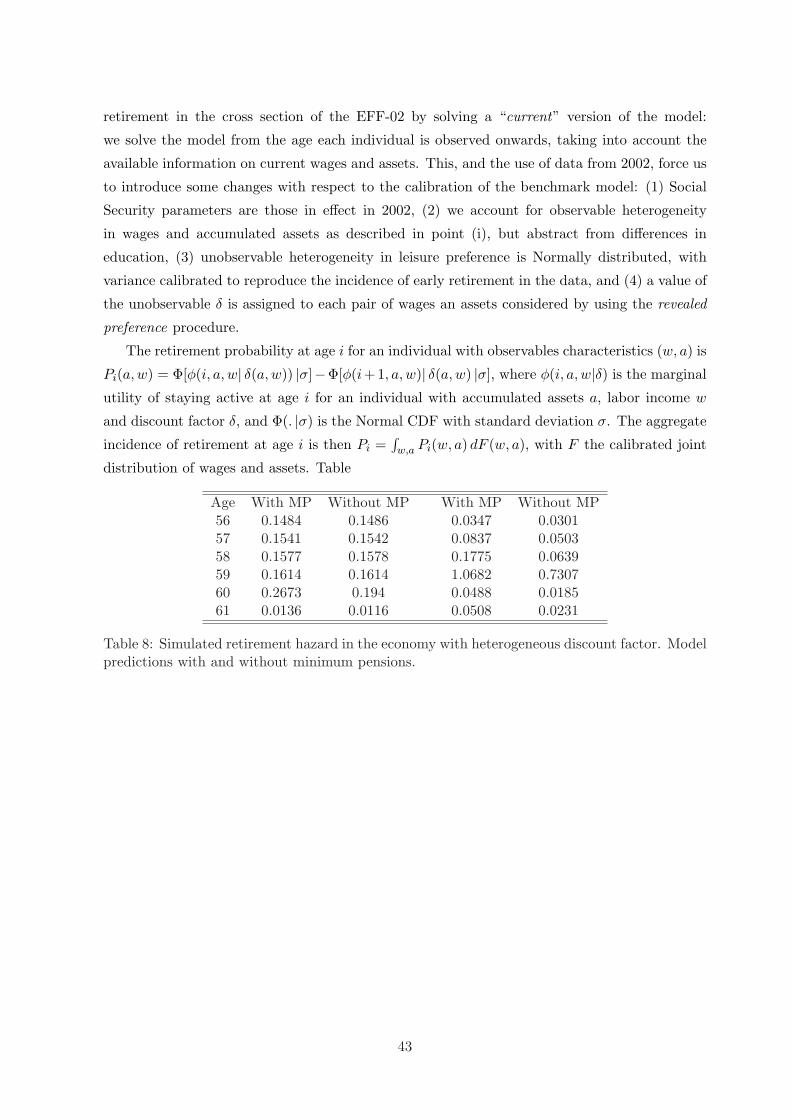
retirement in the cross section of the EFF-02 by solving a “current” version of the model:

we solve the model from the age each individual is observed onwards, taking into account the

available information on current wages and assets. This, and the use of data from 2002, force us

to introduce some changes with respect to the calibration of the benchmark model: (1) Social

Security parameters are those in effect in 2002, (2) we account for observable heterogeneity

in wages and accumulated assets as described in point (i), but abstract from differences in

education, (3) unobservable heterogeneity in leisure preference is Normally distributed, with

variance calibrated to reproduce the incidence of early retirement in the data, and (4) a value of

the unobservable δ is assigned to each pair of wages an assets considered by using the revealed

preference procedure.

The retirement probability at age i for an individual with observables characteristics (w, a) is

Pi(a,w) = Φ[φ(i, a, w| δ(a,w)) |σ]−Φ[φ(i+1, a, w)| δ(a, w) |σ], where φ(i, a, w|δ) is the marginal

utility of staying active at age i for an individual with accumulated assets a, labor income w

and discount factor δ, and Φ(. |σ) is the Normal CDF with standard deviation σ. The aggregate

incidence of retirement at age i is then Pi =∫w,a Pi(w, a) dF (w, a), with F the calibrated joint

distribution of wages and assets. Table

Age With MP Without MP With MP Without MP56 0.1484 0.1486 0.0347 0.030157 0.1541 0.1542 0.0837 0.050358 0.1577 0.1578 0.1775 0.063959 0.1614 0.1614 1.0682 0.730760 0.2673 0.194 0.0488 0.018561 0.0136 0.0116 0.0508 0.0231

Table 8: Simulated retirement hazard in the economy with heterogeneous discount factor. Modelpredictions with and without minimum pensions.

43