an artificial co-stimulation classifier for malicious api - UM

AN ARTIFICIAL CO-STIMULATION CLASSIFIER FOR MALICIOUS API

CALLS CLASSIFICATION IN PORTABLE EXECUTABLE MALWARES

SAMAN MIRZA ABDULLA

THIS THESIS SUBMITTED IN FULFILMENT OF THE REQUIREMENT FOR THE DEGREE OF

DOCTOR OF PHILOSOPHY

FACULTY OF COMPUTER SCIENCE AND INFORMATION TECHNOLOGY UNIVERSITY OF MALAYA

KUALA LUMPUR MALAYSIA

2012

UNIVERSITY OF MALAYA

ORIGINAL LITERARY DECLARATION

Name of Candidate: Saman Mirza Abdulla I.C. Passport: S974411

Registration metric number: WHA080028

Name of Degree: Doctor of Philosophy (PhD)

Title of the thesis: An Artificial Co-stimulation Classifier for Malicious API Calls

Classification in Portable Executable Malwares

Field of study: Artificial Classifier Models for Malware Classification

I do solemnly and sincerely declare that:

(1) I am the sole author/writer of this work;

(2) This work is original;

(3) Any use of any work in which copyright exists was done by way of fair dealing

and for permitted purposes and any excerpt or extract form, or reference to or

reproduction of any copyright work has been disclosed expressly and

sufficiently and the title of the work and its authorship have been acknowledged

in this work;

(4) I do not have any actual knowledge nor do I ought reasonably to know that the

making of this work constitutes an infringement of any copyright work;

(5) I hereby assign all and every rights in the copyright to this work to the

University of Malaya (‘UM’), who henceforth shall be owner of the copyright in

this work and that any reproduction or use in any form or by any means

whatsoever is prohibited without the written consent of UM having been first

had and obtained;

(6) I am fully aware that if in the course of making this work I have infringed any

copyright whether intentionally or otherwise, I may be subject to legal action or

any other action as may be determined by UM.

Candidate’s Signature: Date: 12h April 2013

Subscribed and solemnly declared before.

Witness’s Signature: Date: 12h April 2013

Name:

Designation:

iii

ABSTRACT

Recently, most researchers have employed behaviour based detection systems to

classify Portable Executable (PE) malwares. They usually tried to identify malicious

Application Programming Interface (API) calls among the sequence of calls that made

by a suspected application. They depended mostly on measuring the similarity or the

distance between the suspected API calls with a set of predefined calls that collected

from normal and malware applications. However, malwares always tried to keep their

normality through hiding their malicious activities. Within such behaviours, calls that

made by PE malwares become more similar to normal, which in turn, challenging most

distinguishing models. Even such similarity puts the accuracy of most classifier models

in a very critical situation as many misclassified and doubtful results will be recorded.

Therefore, this work has addressed the accuracy problem of the API call behaviour

classifier models. To achieve that, the work has proposed a biological model that

defined as Artificial Costimulation Classifier (ACC). The model can mimic the

Costimulation phenomenon that occurred inside the Human Immune Systems (HIS) to

control errors and to avoid self-cell attacking. Moreover, Costimulation can work as

safety and balance processes inside the Artificial Immune System (AIS).

To build the ACC model, this work has employed the Feed forward Back-Propagation

Neural Network (FFBP-NN) with Euclidean Distance. The work also used the K-fold

cross validation method to validate the dataset. The results of our work showed the

ability of the ACC model to improve the accuracy of malicious API call classification

up to 90.23%. The results of the ACC model have been compared with four types of

classifier models and it shows its outperformance.

iv

ABSTRAK

Pada masa ini, kebanyakan penyelidik telah menggunakan sistem pengesan perilaku

untuk mengklasifikasikan Portable Executable (PE) malware. Mereka kebiasaanya

mencuba untuk mengenalpasti panggilan API kod hasad sebagai jujukan panggilan yang

dibuat oleh aplikasi yang mencurigakan. Mereka amat bergantung kepada pengukuran

persamaan atau jarak antara panggilan API yang dicurigai dengan set panggilan

pratakrif yang dikumpukan dari aplikasi normal dan hasad. Namun, perision hasad

kebiasaanya berusaha untuk menjaga normality dengan menyembunyikan aktiviti

subversif mereka. Dalam perilaku seperti ini, panggilan yang dibuat malware PE hasad

menjadi lebih mirip dengan panggilan normal yang mengelirukan model pengkelasan.

Bahkan, persamaan ini meletakkan ketepatan kebanyakan model pengkelasan dalam

situasi yang kritikal kerana banyak kesilapan dalam pengkelasan dan hasil yang diragui

direkodkan. Oleh yang demikian, penulisan ini mensasarkan ketepatan masalah dalam

perilaku panggilan API model pengkelasan. Untuk mencapai matlamat ini, kajian ini

mencadangkan model biologi yang didefinasikan sebagai Artificial Costimulation

Classifier (ACC). Model ini dapat meniru fenomena Costimulation di dalam Sistem

Imun Manusia (HIS) bagi mengawal kesilapan dan mengelakkan serangan sesama sel.

Costimulation boleh berfungsi sebagai proses keselamatan dan pengimbangan di dalam

Imun Sistem Buatan (AIS). Untuk membina model ACC, kajian ini telah menggunakan

Feedforward Back-Propagation Neural Network (FFBP-NN) dengan Euclidean

Distance. Kajian ini juga turut menggunakan pendekatan K-fold cross validation untuk

menguji set data. Hasil penemuan daripada kajian ini menunjukkan kemampuan model

ACC untuk memperbaiki ketepatan pengkelasan panggilan API kod hasad sehingga

90%. Hasil daripada model ACC ini telah dibandingkan dengan empat model

pengkelasan dan menunjukkan hasil yang memberangsangkan.

v

ACKNOWLEDGMENTS

It is the time for appreciating the role of some people that contributed directly or

indirectly to achieve this thesis. However, the author wants to start firstly to thank the

God for his gracious and merciful through achieving this work, and he always praying

him for these mercies and blessings.

Secondly, the author wants to send a special appreciation to his supervisors, Assoc.

Prof. Dr. Miss Laiha Mat Kiah and Assoc. Prof. Dr. Omar Zakaria, for their great

supports.The author wants to state here that only their suggestions and comments, with

support from Allha, werethe reasons to build a work like this thesis from a scratched

project proposal.

For management and financial supports, the author wants to thank the Ministry of

Higher Education and Scientific Research of KRG with Mr. Ahmed Ismail. The author

wants to send the same thank to University of Malaya, Faculty FCSIT, department of

Computer System and Technology, and all UM staffs for providing the required

facilities and supports.

Finally, the author wishes to express her love and gratitude to her beloved families; for

their understanding and endless love, through the duration of his studies. The author

wants to mention the role of two family members that supported him during his study;

the brother Mr. Srood Mirza and the wife Rozhan Dilshad, and he feels that they

deserve to dedicate this study to them.

vi

DEDICATION

This thesis is dedicated to:

To My father and mother;

To my faithful brother SROOD and my lover wife ROZHAN;

and

To my Kids:

SAKO, SANAR and SAN

vii

ORIGINAL LITERARY DECLARATION .................................................................... II

ABSTRACT .................................................................................................................... III

ABSTRAK ...................................................................................................................... IV

ACKNOWLEDGMENTS ............................................................................................... V

DEDICATION ................................................................................................................ VI

LIST OF FIGURES ......................................................................................................... X

LIST OF TABLES ........................................................................................................ XII

LIST OF ABBREVIATION ........................................................................................ XIII

CHAPTER ONE ............................................................................................................... 1

1. RESEARCH ORIENTATION ...................................................................................... 2

1.1 INTRODUCTION AND BACKGROUND ...................................................................... 2

1.2 THE MOTIVATION OF THE RESEARCH ................................................................... 6

1.3 THE PROBLEM STATEMENTS ................................................................................. 8

1.4 THE RESEARCH QUESTIONS ................................................................................ 12

1.5 THE OBJECTIVES OF RESEARCH .......................................................................... 13

1.6 THE SIGNIFICANT OF THE STUDY ........................................................................ 14

1.7 THE SCOPE OF THE RESEARCH ............................................................................ 15

1.8 ORGANIZATION OF THIS STUDY ........................................................................... 16

CHAPTER 2 ................................................................................................................... 17

2. CLASSIFICATION OF MALICIOUS API CALLS IN PE MALWARES:

LITERATURE REVIEW................................................................................................ 17

2.1 INTRODUCTION AND BACKGROUND .................................................................... 17

2.2 COMPUTER SECURITY ......................................................................................... 19

2.3 COMPUTER MALWARES ...................................................................................... 20

2.4 CLASSES AND BEHAVIOURS OF MALWARES ....................................................... 22

2.5 PE MALWARES ................................................................................................... 23

2.5.1 PE Format ................................................................................................... 24

2.5.2 The Vulnerabilities in PE Format ............................................................... 29

2.6 ABUSING API FUNCTION BEHAVIOURS OF PE MALWARES................................. 32

2.7 CLASSIFICATION OF API CALLS BEHAVIOURS .................................................... 34

2.8 REVIEW ON MALICIOUS API CALLS CLASSIFIER MODELS .................................. 36

2.8.1 Non-Biological API Detection Models........................................................ 39

2.8.2 Biological API detection systems ................................................................ 47

2.8.3 Why Biological Models? ............................................................................. 55

2.9 WORK STRATEGY OF HIS: .................................................................................. 56

2.9.1 Important Activities of HIS.......................................................................... 59

2.9.2 Co-stimulation Function in HIS .................................................................. 61

2.10 ARTIFICIAL CO-STIMULATION CLASSIFIER (ACC): ............................................. 64

2.10.1 ANN Classifier Technique: ......................................................................... 67

2.10.2 The Similarity Measuring Technique: ......................................................... 72

2.11 CHAPTER SUMMARY ........................................................................................... 74

viii

CHAPTER 3 ................................................................................................................... 75

3. RESEARCH METHODOLOGY ................................................................................ 75

3.1 INTRODUCTION ................................................................................................... 75

3.2 METHODOLOGY FLOW ........................................................................................ 76

3.3 PART ONE: PE SAMPLES AND API CALL VECTORS ........................................... 77

3.3.1 The Properties of PE Malware Samples ..................................................... 79

3.3.2 The Sources of PE Samples ......................................................................... 82

3.3.3 PE Samples Verification Process ................................................................ 83

3.3.4 Extracting API Functions (Execution of PE Samples) ................................ 86

3.3.5 API Function Referencing File ................................................................... 89

3.3.6 Indexing the observed API Functions ......................................................... 91

3.3.7 Scanning –Sliding the Indexing API calls ................................................... 92

3.3.8 Labelling vectors in X1 and X2:.................................................................. 96

3.4 PART TWO: SIGNAL-1 AND SIGNAL-2 GENERATION .............................................. 97

3.4.1 Signal-1 generation ..................................................................................... 98

3.4.2 Signal-2 generation ................................................................................... 101

3.5 PART THREE: CO-STIMULATION........................................................................ 102

3.6 MODEL AND PROBLEM’S VALIDATION ............................................................. 104

3.7 CHAPTER SUMMARY ......................................................................................... 105

CHAPTER 4 ................................................................................................................. 106

4- ACC IMPLEMENTATION ................................................................................... 106

4.1 INTRODUCTION: ................................................................................................ 106

4.2 SYSTEM ENVIRONMENT AND EMPLOYED SOFTWARE ........................................ 107

4.3 ACC IMPLEMENTATION: PART ONE ................................................................. 108

4.3.1 Properties of PE Samples ......................................................................... 108

4.3.2 The sources of PE Samples ....................................................................... 109

4.3.3 PE Samples verification process ............................................................... 110

4.3.4 Extracting API Functions (Execution of PE samples): ............................. 111

4.3.5 Preparing dataset X: ................................................................................. 113

4.3.6 Preparing the Matrix X1: .......................................................................... 114

4.3.7 Preparing the Matrix X2: .......................................................................... 116

4.4 PART TWO OF ACC MODEL: ........................................................................... 117

4.4.1 Training and Testing ANN (FFBP-NN): Dataset X1 ................................ 118

4.4.2 Training and Testing ANN (FFBP-NN): Dataset X2 ................................ 122

4.4.3 Active Threshold boundaries: ................................................................... 125

4.4.4 Grouping the Results: ............................................................................... 131

4.5 PART THREE OF ACC MODEL: CO-STIMULATION ........................................... 133

4.5.1 Calculating the Similarity Measurement .................................................. 134

4.5.2 Costimulation process: ............................................................................. 137

4.6 CHAPTER SUMMARY ......................................................................................... 140

CHAPTER 5 ................................................................................................................. 141

5. EVALUATING ACC WITH OTHER CLASSIFIER MODELS ............................. 141

5.1 INTRODUCTION ................................................................................................. 141

ix

5.2 SUPERVISED LEARNING CLASSIFIER MODELS ................................................... 142

5.2.1 Feed-Forward Back Propagation Neural Network (FFBP-NN): ............. 142

5.2.2 Support Vector Machine (SVM): ............................................................... 143

5.3 UNSUPERVISED CLASSIFIER MODEL .................................................................. 144

5.3.1 Self-Organizing Map (SOM): .................................................................... 144

5.3.2 (K-means):................................................................................................. 147

5.4 STATISTICAL CLASSIFIER MODELS .................................................................... 151

5.5 ACCURACY EVALUATION FOR CLASSIFIER MODELS .......................................... 157

5.6 CHAPTER SUMMARY ......................................................................................... 161

CHAPTER 6 ................................................................................................................. 162

6. CONCLUSION AND CONTRIBUTIONS .............................................................. 162

6.1 INTRODUCTION ................................................................................................. 162

6.2 CONCLUSION .................................................................................................... 162

6.3 ACHIEVEMENT OF RESEARCH OBJECTIVES ....................................................... 163

6.4 CONTRIBUTION ................................................................................................. 167

6.5 SUGGESTED FUTURE WORKS ............................................................................. 172

6.6 CHAPTER SUMMARY ......................................................................................... 174

REFERENCES .............................................................................................................. 175

LIST OF PUBLICATION............................ ERROR! BOOKMARK NOT DEFINED.

APPENDIX-1 ................................................................................................................ 186

The letter from Peter Szor ...................................................................................... 186

APPENDIX-2 ................................................................................................................ 188

Codes used throughout building ACC model ......................................................... 188

APPENDIX-3: TRUE AND FALSE RATES IN TESTED MODELS INCLUDED ACC

....................................................................................................................................... 206

x

LIST OF FIGURES

Figure 1-1 Comparison between normal and malware applications in a number of calls

conducted for only six types of API functions .................................................................. 9

Figure 1-2 SOM classification and FA generation ......................................................... 10

Figure 1-3 The Underlined Scopes in this research ......................................................... 15

Figure 2-1 The flow of literature review .......................................................................... 18

Figure 2-2Format of PE applications (HZV, 2010) ........................................................ 25

Figure 2-3Memory block with filled and free space area ................................................ 30

Figure 2-4Using both types of calls to find addresses of an API function ...................... 31

Figure 2-5 Similarity between API calls in two malwares ............................................. 34

Figure 2-6 Layers of the immune system (Michael A. Horan, 1997) ............................ 57

Figure 2-7Parallel actions, signal communications, feedbacks, and confirmation

processes ......................................................................................................................... 61

Figure 2-8 HIS co-stimulation Process (Rang, Dale, Ritter, & Moore, 2003) ................ 63

Figure 2-9 ACC model to classify malicious API calls .................................................. 64

Figure 2-10 Input and output of an ANN neuron ............................................................. 67

Figure 2-11 Three main types of transfer function in ANN ............................................. 68

Figure 2-12 Typical structure of FFBP-NN with n hidden layer and i nodes at output

layer ................................................................................................................................. 69

Figure 3-1 The main parts of the ACC model................................................................. 76

Figure 3-2The activities and steps of part one of the ACC model .................................. 78

Figure 3-3 The applications’ categories the focused by this work as samples ............... 81

Figure 3-4 PE samples verification process .................................................................... 84

Figure 3-5 Phases and rounds of PE sample Execution and API calls extraction .......... 87

Figure 3-6Collecting API functions that are called by a PE application using

APIMonitoring Software ................................................................................................. 88

Figure 3-7 The API function reference file ..................................................................... 90

Figure 3-8 Scanning process and Window Sliding to Build Input Vector ...................... 93

Figure 3-9 Grouping API calls based on Behaviours or Activities of Malwares............ 94

Figure 3-10 Attaching indexing and scanning-sliding steps to extracting API calling step

......................................................................................................................................... 95

Figure 3-11 Aactivities and sub-blocks of part two of ACC model ............................... 97

Figure 3-12 Process of generating Signal-1 .................................................................... 98

Figure 4-1 List of API names converted to equivalent API indexes ............................ 114

Figure 4-2 Sample of X to X1 conversion ...................................................................... 115

Figure 4-3 Example of (X) to (X2) conversion .............................................................. 116

Figure 4-4 The structure of the ANN used as tested classifier model .......................... 118

Figure 4-5 Details about the structure of the ANN used as tested classifier model...... 119

Figure 4-6Training parameters for the FFBP-NN using dataset X1 ............................... 120

Figure 4-7; Training, testing, and validation status for X1 dataset ................................ 121

Figure 4-8The result of predicting (6000) non-seen vectors after training FFBP-NN with

dataset X1tests .................................................................................................................. 121

Figure 4-9 Training, testing, and validation status for X2 dataset .................................. 123

xi

Figure 4-10 The result of predicting (2,000) non-seen vectors after training FFBP-NN

with dataset X2tests .......................................................................................................... 124

Figure 4-11 Confusion matrix for FFBP-NN training and testing with X2tests ............... 124

Figure 4-12 Shifting the threshold line process, and the THREE areas of results. ....... 127

Figure 4-13 The impact of Shifting threshold lines on the RMSE measure of each

defined area ................................................................................................................... 129

Figure 4-14 RMSE for doubtful area increased more than other areas......................... 130

Figure 4-15 Number of high certainty vectors in classes and sub classes .................... 136

Figure 5-1 Confusion matrix for FFBP-NN training and testing with X1tests ................ 142

Figure 5-2 The Confusion matrix output for SVM classifier model ............................. 143

Figure 5-3The physical structure for SOM NN at part one test ..................................... 144

Figure 5-4 Number of vectors inside each cluster (SOM part one test)........................ 145

Figure 5-5 The Confusion matrix for SOM classifier model ....................................... 146

Figure 5-6 Clustering 2000 vectors with K-means algorithm ....................................... 147

Figure 5-7 Confusion Matrix for K-mean classifier model .......................................... 149

Figure 5-8 the variance of distances between vectors and centres................................ 149

Figure 5-9 A sample of the SPSS program report about API call frequencies collection

....................................................................................................................................... 152

Figure 5-10 Samples of vectors that shown the frequency rate of API calls ................ 153

Figure 5-11 Obtaining the average probability measure for API functions .................. 154

Figure 5-12 Median accuracy comparison between the tested classifier models ......... 158

Figure 5-13 The mean accuracy of models that computed using ANOVA testing method

....................................................................................................................................... 159

xii

LIST OF TABLES

Table 2-1Abusing behaviours of API functions by Malware ......................................... 33

Table 2-2 Summary of Related Works for Non-Biological Malware Detection Models 42

Table 2-3 List of Biological Models that Inspired HIS Algorithms and Models............ 50

Table 3-1; Number of Malwares Samples that Analysed and Verified .......................... 85

Table 3-2 Rules that considered during signals confirmation. ...................................... 102

Table 4-1 Number of PE that passed verification ......................................................... 110

Table 4-2A compression result between the number of monitored API functions and

actually called API function .......................................................................................... 112

Table 4-3 The effect of upper and lower line shifting on the RMSE measure in the

defined three area .......................................................................................................... 128

Table 4-4 Impact of increasing the input number on RMSE ........................................ 130

Table 4-5 FP and FN isolating and minimizing RMSE ................................................ 132

Table 4-6 The OAS values for each behaviour class .................................................... 136

Table 4-7 Value of and its percentage for each behaviour class. ............................... 137

Table 4-8 Number of doubtful vectors with RMSE rate improvements after applying co-

stimulation process ........................................................................................................ 138

Table 4-9 Number of vectors in the three predefined areas before and after applying co-

stimulation ..................................................................................................................... 139

Table 5-1 Number of vectors inside and outside the mean distance for each class ..... 150

Table 5-2 FP and FN rates for Statistical Classifier models (Highest and Lowest call

rate similarity) ............................................................................................................... 155

Table 5-3 FP and FN rates for Statistical Classifier models (Probability of malicious

calling rate similarity) ................................................................................................... 156

Table 5-4 The median accuracy comparison between ACC and some classifier models

....................................................................................................................................... 157

Table 5-5 Comparison between the mean of tested and ACC classifier models .......... 160

xiii

LIST OF ABBREVIATION

COMMON NAME ACRONYM

Anti-virus AV

Application programming Interface API

Portable Executable PE

Operating system OS

False Alarm FA

False Positive FP

False Negative FN

Root Mean Square Error RMSE

Immune System IS

Human Immune System HIS

Artificial Immune System AIS

Support Vector Machine SVM

Self-Organizing Map SOM

True Positive TP

Artificial Co-stimulation Classifier ACC

Dynamic link library DLL

Common Object File Format COFF

Relative virtual address RVA

Import address table IAT

Original entry point OEP

Negative selection algorithm NSA

Clonal selection algorithm CSA

Major Histocompatibility Complex MHC

Artificial neural network ANN

Feed forward Back propagation Neural Network FFBP-NN

1

List of Publication

S. M. Abdulla, M. L. Mat Kiah & O. Zakaria. 2012. Minimizing Errors in Identifying

Malicious API to Detect PE Malwares Using Artificial Costimulation. International

Conference on Emerging Trends in Computer and Electronics Engineering

(ICETCEE'2012), pg. 49-54.

Abdulalla, S. M., Kiah, L. M., & Zakaria, O. (2010). A biological model to improve PE

malware detection: Review. [Academic Journal]. International Journal of the Physical

Sciences, 5(15), 12.

Abdulla, S. M., N. B. Al-Dabagh and O. Zakaria (2010). "Identify Features and

Parameters to Devise an Accurate Intrusion Detection System Using Artificial Neural

Network." World Academy of Science, Engineering and Technology (70): 627-631.

Saman Mirza Abdulla, O. Z. (2009). Devising a Biological Model to Detect

Polymorphic Computer Viruses Artificial Immune System (AIM): Review. 2009

International Conference on Computer Technology and Development, Kota Kinabalu,

Malaysia, IEEE Computer Society.

2

Chapter One

1. Research Orientation

1.1 Introduction and Background

Recently, most malware classifier researchers have depended on tracing the behaviours

of malwares rather than looking for knowing signatures (M Alazab, Venkataraman, &

Watters, 2010; Peng, 2011; Wagener, State, & Dulaunoy, 2008). The reasons behind

this trend are going back to the number of malwares that crossed (80) millions

(Spafford, 1990), and the defeat techniques (Polymorphic and Metamorphic) that used

by malwares to change old malwares’ signature to new ones. Although these two

reasons have challenged signature based classifier models, they have encouraged

malware classifier researchers to employ the behaviour based classifier models rather

than other types of malware classifier model (Y. Hu, Chen, Xu, Zheng, & Guo, 2008;

Lanzi, Sharif, & Lee, 2009; Park & Reeves, 2011; Tian, Islam, Batten, & Versteeg,

2010; Trinius, Willems, Holz, & Rieck, 2011; Zolkipli & Jantan, 2011).

The fundamental work of any type of behaviour-based classification system depends on

learning the behaviours of known malwares and subsequently scanning other

applications to detect similar behaviours (Cohen, 1987). Along this direction,

researchers have studied the behaviours of numerous malwares to build different kinds

of behaviour-based classifier systems. The memory access behaviour, the codes that are

more frequently used by malwares, and the system files that register record-

modification activities are among the behaviours that frequently studied by researchers

to build different kinds of behaviour-based detection systems (Ding, Jin, Bouvry, Hu, &

Guan, 2009; H. J. Li, Tien, Lin, Lee, & Jeng, 2011; Rieck, Holz, Willems, Düssel, &

3

Laskov, 2008; Rozinov, 2005; Wang, Pang, Zhao, & Liu, 2009; Yoshiro Fukushima,

Akigiro Sakai, Yoshiaki Hori, & Sakurai, 2010; C. W. J. P. R. Zhao & Liu, 2009).

One of the most important behaviour that researchers have focused more is monitoring

and tracing the behaviours of application programming interface (API) calling. This

behaviour is utilized to build API call behaviour-based detection systems. This

monitoring system is employed more frequently because malwares, as normal

applications, should call API functions during implementation. Based on different ways

of calling, API call behaviour-based classifier systems, ideally, can identify malicious

calls among normal calls. As a result, the classifier system can reveal the behaviour of

malwares in applications (M. Alazab, Layton, Venkataraman, & Watters, 2010; M

Alazab et al., 2010; Bai, Pang, Zhang, Fu, & Zhu, 2009; Cheng Wang, 2009; S. Choi,

Park, Lim, & Han, 2007; Dabek, Zhao, Druschel, Kubiatowicz, & Stoica, 2003;

Dunham, 2011; Focardi, Luccio, & Steel, 2011; K.-S. Han, Kim, & Im, 2011; J-Y. Xu,

2004; Kwon, Bae, Cho, & Moon, 2009; Miao, Wang, Cao, Zhang, & Liu, 2010; Nakada

et al., 2002).

The calling behaviours that classified by an API calls classifier model can be extracted

from some specific fields inside Portable Executable (PE) file format(Microsoft, 2008).

PE is a type of the file format that followed by a wide range of applications, especially,

the ones that can be executed under Windows Operating System (OS) (Y. Huang,

2003). This application’s format has some fields where the name and the address of the

required API functions that called by an application during its execution can be found

(APIMonitoring.Com, 2010). Malwares as normal applications can keep the addresses

of the required API functions in these fields and can use these addresses to find any API

function that necessary during their execution.

4

Malwares that can infect any PE applications are known as PE malwares, which also

known as Win32 malwares (Bradfield, 2010). PE malwares can call API functions as

normal PE applications do, and Windows OS responds to PE malwares’ calls as its

respond to normal PE applications. Windows OS cannot make any differentiate between

the calls that made by PE malwares and PE normal applications (Szor, 2000). This

situation encouraged PE malwares to misuse or abuse these API functions, and to hide

their malicious activities from behaviour classifier models. For instance, the API

function RegQueryValuExA ( ) that called during installation of new PE applications,

probably can be called by PE Trojan horse malwares to conduct communication with

their resources so that they can get new updates. Therefore, a classifier model cannot

easily decide either calling such functions is for malicious purposes or it is normal.

Accordingly, cases like this call are either misclassified or correctly classified but with a

low certainty degree (doubtfully classified) (K. S. Han, Kim, & Im, 2012b). This

situation affects negatively on the accuracy degree of any classifier models.

The accuracy of classifier models is directly affected by errors that may occur during

the process of classifying objects. Errors, which mean misclassifying objects or objects

that doubtfully classified, can be measured by computing parameters in two directions.

In the first direction, the two types of False Alarms (FA), False Positive (FP) and False

Negative (FN), should be obtained. This direction determines the number of objects that

are incorrectly classified. The second direction defines the level of certainty with

respect to the correct classification of objects. To obtain a high degree of certainty,

classifier models usually depend on computing of the Root Mean Square Error (RMSE)

(Yoshiro Fukushima et al., 2010). With respect to both directions, API call classifier

models have low accuracy because they have a high FA rate, which indicates

misclassification, and have high RMSE rate, which means objects have been classified

doubtfully.

5

Researchers, in the past years, employed many tools and techniques to build API calling

behaviour classifier models, although they have high FA and RMSE rates’ problem (M.

Alazab, Venkatraman, & Watters, 2011; Fei Chen, 2009; Marhusin, Larkin, Lokan, &

Cornforth, 2008; Miao Wang, 2009; Sami, Yadegari, Peiravian, Hashemi, & Hamze,

2010). In each work, researchers have looked for different solutions to overcome the

accuracy problems. Moreover, researchers studied different parts of API behaviour-

based detection systems to obtain features that more relevant to the accuracy problem

(Father, 2004; Kwon et al., 2009). Accordingly, researchers proposed different API

calling behaviour classifier models (K. S. Han, Kim, & Im, 2012a; Islam, Islam, &

Chowdhury, 2012). Researches, even, tried to find some bio-oriented solutions from the

Immune System (IS) algorithms to improve the accuracy of API calls classifier models

(Khaled, Ab d ul-Kader, & Ismail, 2010). Bio-oriented models, sometimes referred as

biological models, are inspired by several phenomena and algorithms that occur inside

the Human Immune System (HIS) (Abdulalla, Kiah, & Zakaria, 2010; Zakaria, 2009).

Since 1994, when the idea of the biological model was coined, different IS algorithms,

such as Negative Selection, Clonal Selection, and Danger Method, have been widely

used in different works and fields, particularly in malware detection models(Jieqiong

Zheng 2010). Most IS algorithms depend on pattern-recognition and shape-matching

processes. Many researchers found that biological models suffer from a high rate of FA

(Xiao & Stibor, 2011). The most recent algorithm, Dendretic Cell Algorithm, which is

considered as a second-generation algorithm for Artificial Immune System (AIS), has a

problem in setting an appropriate threshold value for classifier models (Xiao & Stibor,

2011). Hence, all AIS algorithms based models that used to classify malicious API calls

need accuracy improvement as well.

To provide this improvement, the current work intends to find a method that can control

errors. The present work has found that a biological phenomenon, which is called co-

6

stimulation and occurs inside IS, has been utilized as an error controller. The IS uses

this biological error controller to eliminate errors occurred when a self-cell is classified

as non-self-cell. This process means minimizing FA rates inside IS. Further, the

phenomenon does not occur independently; it always comes in parallel with other IS

activities to improve the detector’s ability (D Dasgupta, 2007). For this reason, this

phenomenon is defined as a safety and balancing procedure within the work of AIS

(Jieqiong Zheng 2010). Therefore, this present research proposes employing the

functionalities of this phenomenon to overcome the exist drawbacks in the malicious

API call classifiers.

The aim of utilizing the concept of this phenomenon in malicious API call classification

is to control the errors first, and subsequently start implementing improvements. The

improvements that the current work intends to apply include increasing the certainty of

objects that are doubtfully classified, which subsequently means improvement of the

RMSE. The improvements also included minimizing the misclassification rate, and

consequently, means decreasing the FA rate. As a result the accuracy can be improved.

1.2 The Motivation of the Research

Many recent studies have traced and analysed API calls that were made by suspected

applications to detect and identify the PE malwares inside computer systems (M. Alazab

et al., 2010; M Alazab et al., 2010; Miao et al., 2010; Sami et al., 2010). These were

performed because malwares can bypass the valid AV software and can challenge them

by using different signature-defeating techniques (M. Alazab et al., 2011). Secondly,

with defeating techniques, such as encryption and polymorphic techniques, malwares

can make changes on malware signatures but cannot make any changes on the type and

the sequence of API calls (J-Y. Xu, 2004). In addition, any cancellation, deletion, or

7

modification of an API function during a PE execution would generate an end error

message (Father, 2004). Therefore, the type and the way that API functions, as called by

any PE malware, will not be changed even if the signature or the structure of codes has

been modified. Furthermore, malwares should call the required API functions in order

to be executed smoothly and correctly (Zhu & Liu, 2011; Zolkipli & Jantan, 2011). All

above confirmed that for each malware a sequence of API functions is existed, and this

sequence cannot be encrypted or changed for a specific malware unless the behaviour

and the codes of the malware is changed totally (Szor, 2006).

API behaviour-based detection systems have effective features and characteristics for

classifying malicious API calls. The systems can nullify the effect of many defeating

techniques and can provide indication on existing malicious API calls. More

justifications have been structured and organized to explain the trends in using API call

monitoring (Bayer, Habibi, Balzarotti, Kirda, & Kruegel, 2009; Peng, 2011; Tabish,

Shafiq, & Farooq, 2009; H. Zhao, Zheng, Li, Yao, & Hou, 2009; Zhu & Liu, 2011).

However, malwares usually challenge these trends by making their behaviour of calling

API functions appear as normal. Malwares use the same procedures and ways to call

API functions to hide their malicious and non-privileged behaviours from detection

systems and the users’ eyes. Malwares try to display themselves as normal as possible

by following the call sequences of some normal APIs (F. Y. Zhang, Qi, & Hu, 2011a).

These malware behaviours negatively affect most malicious API call classifiers, and

lead to misclassify cases as well as doubtfully classify objects, which in turn, puts the

accuracy at a weak level. The existing similarity of API call sequences between normal

and malware applications affects the accuracy of most malicious API call classifiers.

By solving the similarity problem and improving the accuracy, API behaviour classifier

models can attain relevant features and characteristics. Therefore, the current work

8

offers a bio-oriented solution that can improve the discrimination between two different

cases that have similarity in behaviours. The present work can insert a part that is

missed in most malicious API call classifiers, and can bring about improvement in

accuracy. Furthermore, classifier techniques that are applied to sensitive cases or have

numerous doubtful points can depend on the proposed model to achieve accurate

results. By evaluating malwares, this work offers a new definition that explains

malwares more at the detection stage. The proposed new version of malware definition

can help malware analysts, and can explain malwares from the viewpoint of detection

systems.

1.3 The Problem Statements

This research work targets to address the accuracy problem of the classifier models that

distinguish malicious API calling behaviours. The work evaluates different types of

malicious API calling classifier models with respect to the three types of features that

are relevant to the accuracy problem. The features are False Positive (FP), False

Negative (FN) and Root mean Square Error (RMSE).

The accuracy of any malicious API classifier models will be affected negatively when

they classify a malicious API sequence that has some similar characteristics with

normal API sequences. Moreover, when a classifier model depends on some statistical

measures, such as probability or frequency, their accuracy will be also affected

negatively when the probability or frequency measure of a malicious API call came

within the same range that a normal API call has. These problems are clearly illustrated

in Figure 1-1 and Figure 1-2.

9

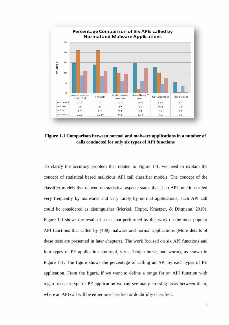
Figure ‎1-1 Comparison between normal and malware applications in a number of

calls conducted for only six types of API functions

To clarify the accuracy problem that related to Figure 1-1, we need to explain the

concept of statistical based malicious API call classifier models. The concept of the

classifier models that depend on statistical aspects states that if an API function called

very frequently by malwares and very rarely by normal applications, such API call

could be considered as distinguisher (Merkel, Hoppe, Kraetzer, & Dittmann, 2010).

Figure 1-1 shows the result of a test that performed by this work on the most popular

API functions that called by (400) malware and normal applications (More details of

these tests are presented in later chapters). The work focused on six API functions and

four types of PE applications (normal, virus, Trojan horse, and worm), as shown in

Figure 1-1. The figure shows the percentage of calling an API by each types of PE

application. From the figure, if we want to define a range for an API function with

regard to each type of PE application we can see many crossing areas between them,

where an API call will be either misclassified or doubtfully classified.

10

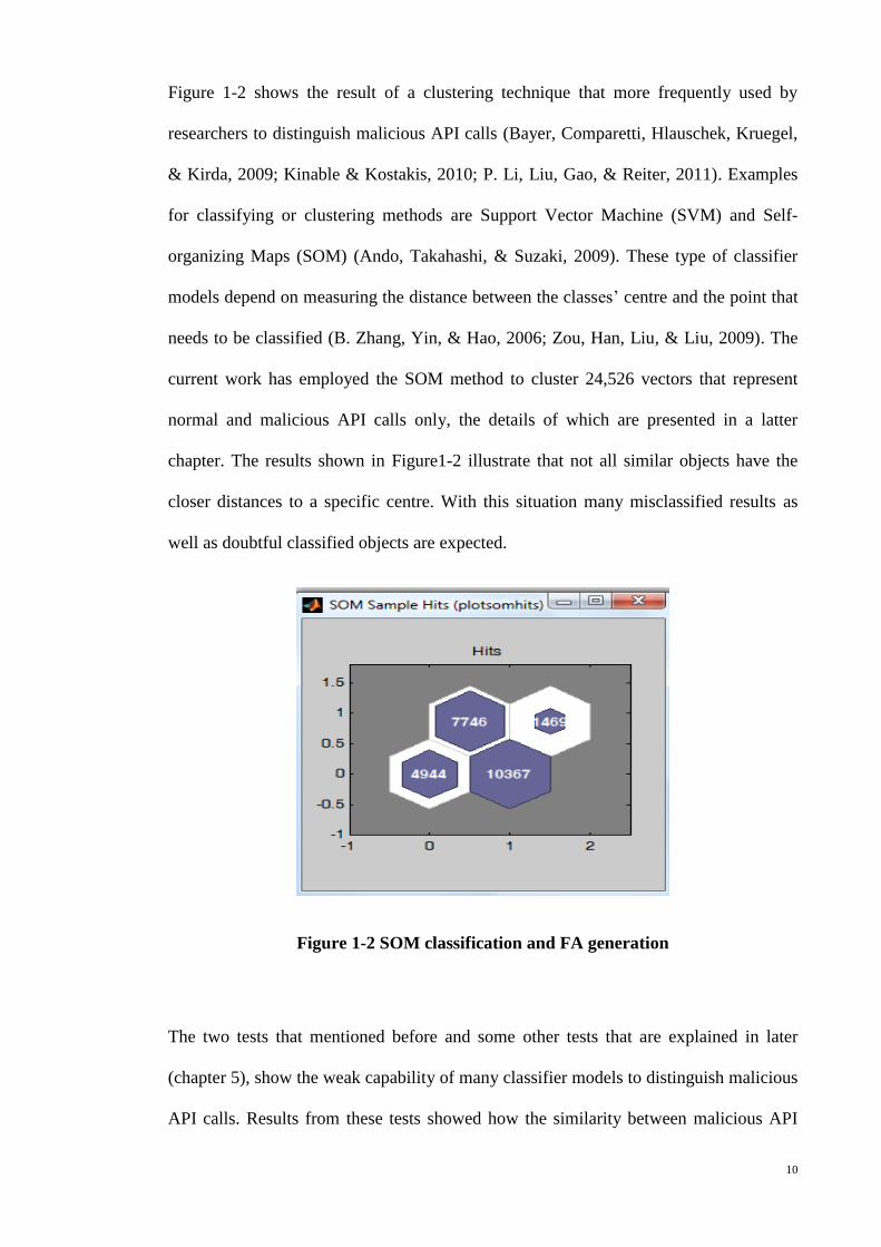
Figure 1-2 shows the result of a clustering technique that more frequently used by

researchers to distinguish malicious API calls (Bayer, Comparetti, Hlauschek, Kruegel,

& Kirda, 2009; Kinable & Kostakis, 2010; P. Li, Liu, Gao, & Reiter, 2011). Examples

for classifying or clustering methods are Support Vector Machine (SVM) and Self-

organizing Maps (SOM) (Ando, Takahashi, & Suzaki, 2009). These type of classifier

models depend on measuring the distance between the classes’ centre and the point that

needs to be classified (B. Zhang, Yin, & Hao, 2006; Zou, Han, Liu, & Liu, 2009). The

current work has employed the SOM method to cluster 24,526 vectors that represent

normal and malicious API calls only, the details of which are presented in a latter

chapter. The results shown in Figure1-2 illustrate that not all similar objects have the

closer distances to a specific centre. With this situation many misclassified results as

well as doubtful classified objects are expected.

Figure ‎1-2 SOM classification and FA generation

The two tests that mentioned before and some other tests that are explained in later

(chapter 5), show the weak capability of many classifier models to distinguish malicious

API calls. Results from these tests showed how the similarity between malicious API

11

calls and normal API calls negatively affect the accuracy of classifier models. The low

accuracy is caused by the continuous inclusion of misclassified and doubtful points by

the output from classifying malicious API calls with normal API calls.

The main improvement that this work aims to achieve is to minimize the FP, FN and

RMSE rates. As these three features have inverse relation with accuracy, minimizing the

rates of these features means improving the accuracy. Moreover, to improve the rate of

these features another problem should be solved, which is the instability of the threshold

value that used as a distinguisher in malicious API calling classifier models. The

outcomes of the clustering and classification based models are generally compared with

a threshold value to distinguish and discriminate cases. Researchers have defined a

value between 0.5 and 0.65 to formulate the threshold value (K. S. Han et al., 2012b;

Zolkipli & Jantan, 2011). Even within this range, however, tests and evaluations

showed that results are not clear with regard to misclassification points. Researchers

usually change this value to minimize the FA rate and to improve the accuracy (Bayer,

Comparetti, et al., 2009; Kinable & Kostakis, 2010; P. Li et al., 2011). Therefore, the

aim of this work is also to present a new formula that enables a threshold value to work

as an error controller beside case distinguisher.

12

1.4 The Research Questions

This research intends to improve the accuracy of malicious API call-classifier models

through using a bio-oriented solution. Therefore, the main question that this work wants

to answer is how to devise an artificial classifier model which exactly can imitate an

accurate biological classifier phenomenon. Other questions that this work wants to

address in regard to this are:

1. What are the problems in the malicious API calls classifier models that led to

misclassify objects or doubtfully classifying objects?

2. Which biological phenomenon is used by human Immune System (IS) as a

classification error controller?

3. What is the suitable tool or technique that can function as an artificial error

controller?

4. How the artificial error controller can function within an artificial classifier

models?

5. How is the effectiveness of the proposed ACC classifier model?

13

1.5 The Objectives of Research

The main objective of this work is to develop a bio-oriented model that can minimize

the FP, FN and RMSE rates in malicious API calls classifier models. In order to achieve

the main objective, this work focuses on the following sub-objectives:

1. To study the relevant literatures on the API behaviour classifier models with

respect to their accuracy;

2. To determine a biological phenomenon that can avoid errors during classifying

biological objects or cells;

3. To propose an appropriate artificial error controller;

4. To develop an Artificial Co-stimulation Classifier (ACC) model; and

5. To test and evaluate the developed ACC model.

14

1.6 The Significant of the Study

The study of classifying PE malwares with normal applications took another direction

during the past years. Instead of investigating the detection of unseen signatures,

researchers proposed different studies to reveal unseen PE malwares through classifying

their API calling behaviours(Fu, Pang, Zhao, Zhang, & Wei, 2008; K. S. Han et al.,

2012a; Kwon et al., 2009; Sami et al., 2010; M. K. Shankarapani, Ramamoorthy,

Movva, & Mukkamala, 2011). Through their studies, researchers have proposed

different classifier models, and they employed different methods to distinguish

malicious API calls. However, the behaviours’ similarity between normal and malware

applications in calling API functions and system’s responding always challenges this

direction of researching as an open source problem. This is because the existing

behaviour’s similarities puts many API calling cases in a doubtful area or misclassified

them. As a result, it impacts negatively on the accuracy of the classifier models.

The project’s goal that designed by this work is for improving the accuracy of the

malicious API calling classifier models. Through achieving this goal, the new direction

of malware classification studies could be taken to better level of accuracy. Moreover,

projects that need to classify different objects that have similar characteristics can get

benefit from the proposed design.

The goal that proposed by this work can be achieved through implementing a new bio-

oriented model. The proposed model, ACC, extracted from the functionality of a

biological phenomenon that called co-stimulation. The phenomenon is occurred inside

Human Immune System (HIS). Therefore, this work introduces a new functionality in

the field of artificial immune system that supports, in general, pattern recognition

projects, especially, the biological based projects.

15

1.7 The Scope of the Research

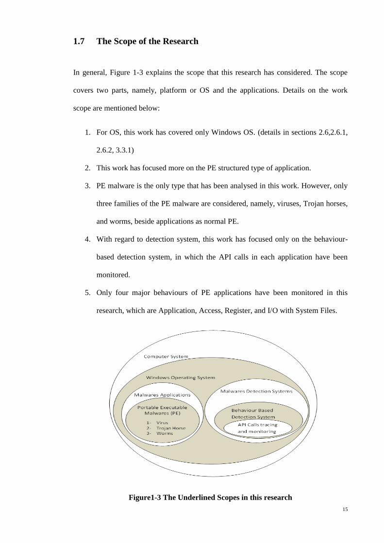
In general, Figure 1-3 explains the scope that this research has considered. The scope

covers two parts, namely, platform or OS and the applications. Details on the work

scope are mentioned below:

1. For OS, this work has covered only Windows OS. (details in sections 2.6,2.6.1,

2.6.2, 3.3.1)

2. This work has focused more on the PE structured type of application.

3. PE malware is the only type that has been analysed in this work. However, only

three families of the PE malware are considered, namely, viruses, Trojan horses,

and worms, beside applications as normal PE.

4. With regard to detection system, this work has focused only on the behaviour-

based detection system, in which the API calls in each application have been

monitored.

5. Only four major behaviours of PE applications have been monitored in this

research, which are Application, Access, Register, and I/O with System Files.

Figure‎1-3 The Underlined Scopes in this research

16

1.8 Organization of this study

The flow between each chapter and inside each chapter is summarized as below:

1. In general, there are four sections in chapter 2:

a. A section is related more on the current behaviour based and API

calls monitoring models that used to detect malicious API and PE

malwares.

b. Another section illustrates the current biological algorithms and

artificial immune system works that proposed as malware detection

systems.

c. A section illustrates the biological functionalities and activities of

HIS.

d. Last section shows the details of the theories and methods that used

by this work to build and simulate the ACC model.

2. Chapter 3 is more related to the methodology of this work. It explains the main

framework of the ACC model. The chapter gives more details about each part of

the ACC model. The functionality of each part and the theory that used to

achieve each part are also explained.

3. Chapter 4 illustrated the execution parameters and characteristics of each part in

the ACC mode. It includes the results that obtained through model execution.

4. Chapter 5 shows testing some major classifier models. Through this chapter, this

work has evaluated results that have been obtained for testing these models. A

compression between the tested classifier models and ACC modes has been

illustrated in this chapter.

5. Chapter 6 explains the conclusion and contributions of this research. The chapter

also explains the achievements of the current research.

17

Chapter 2

2. Classification of malicious API calls in PE malwares: Literature

Review

2.1 Introduction and Background

Malwares are increasingly infecting more PE applications. As these applications

supported by all versions of the Windows platform (Symantec, 2010), and malware

authors easily find new vulnerabilities in such file structures. The PE structure has many

fertile fields that malwares can use for hiding codes and data (Hamlen, Mohan, &

Wartell, 2010). Moreover, Windows dynamically loads and maps all applications to the

main memory. This platform also provides all required dynamic link library (DLL)

functions to any application during execution. Such facilities smoothly and correctly

execute any application, even malwares (Dabak, Phadke, & Borate, 1999; Schreiber,

2001). Moreover, the facility allows PE malwares to become parts of the system. Thus,

the integrated malwares can abuse system resources to propagate. Malwares can then

easily exploit OS vulnerabilities through executor infection.

Valid detection systems that reveal malwares face many challenges. First, unknown PE

malwares can easily defeat signature-based detection systems (S. Yu, Zhou, Liu, Yang,

& Luo, 2011). Therefore, behaviour-based detection systems can offer a ray of hope for

the detection of unseen malwares. However, the accuracy of behaviour-based detection

systems needs to be improved because these systems depend on discriminating normal

behaviours from abnormal ones. In most cases, many overlapping areas exist. Such

similarities in behaviour result in weak classification and detection.

18

This chapter covers subjects relevant to the main targets of our work. These subjects are

divided into two classes related to a specific field. The first field is computer security;

more precisely, computer malware and detection systems. This part concerns PE

malware with behaviour-based detection systems that trace and monitor API calls. The

second field is the biological field, which concerns the HIS phenomenon. This review

intends to support the search for a bio-oriented approach that would improve the

accuracy of classifying malicious API calls in PE applications.

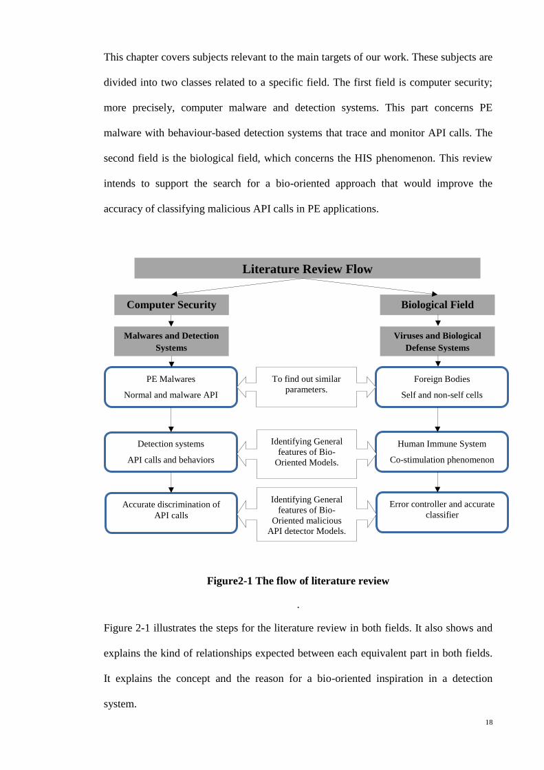
Figure‎2-1 The flow of literature review

.

Figure 2-1 illustrates the steps for the literature review in both fields. It also shows and

explains the kind of relationships expected between each equivalent part in both fields.

It explains the concept and the reason for a bio-oriented inspiration in a detection

system.

Error controller and accurate

classifier

Human Immune System

Co-stimulation phenomenon

Foreign Bodies

Self and non-self cells

PE Malwares

Normal and malware API

calls

Detection systems

API calls and behaviors

Accurate discrimination of

API calls

Literature Review Flow

Computer Security Biological Field

Malwares and Detection

Systems

Viruses and Biological

Defense Systems

To find out similar

parameters.

Identifying General

features of Bio-

Oriented Models.

Identifying General

features of Bio-

Oriented malicious

API detector Models.

19

2.2 Computer Security

Computer security is a branch of computer systems known as information security.

Although it is difficult to describe and specify a definition for computer security, in the

context of computer science, it is almost meaning protecting and preventing accessing

and altering information by unauthorised users (Salomon, 2010). Based on the areas

associated with, computer security covered three main topics:

1- Confidentiality; which means accessing information only by authorised person.

2- Integrity; information should not be altered by unauthorised person in such a

way that authorised users cannot detect it.

3- Authentication; means users are the authorised persons.

This work more concerned to keep integrity in computer security systems as malwares,

which are unwanted or unauthorised softwares, can access and alter information inside

the system in undetectable ways (Szor, 2006).

Computer security has some functions such as detection, prevention, and recovery that

usually used to analyse what the security system can do (Solomon, 1993). However, in

this work the detection function is more concerned as the work deals with infected PE

applications.

Finally, computer security systems have some domains that define the level they can

work there. Each domain mutually depends on one or some other domains. For instant,

this work is more concerned with system security and network security domains

because they related more with unwanted softwares that use networks to change system

files and integrity.

http://en.wikipedia.org/wiki/Information_security

20

Next section gives more details about those unwanted softwares which known as

computer malwares, which they have ability to breach system security and alter system

integrity.

2.3 Computer Malwares

The term “malware” covers all malicious types of software that are used for unwanted

applications (Idika & Mathur, 2007). Although the term malware, which is shortened

from malicious software, was coined to cover all types of unwanted applications, most

computer end-users continue to use the term computer virus, instead of malwares, for

unwanted software, such as Trojan horses and worms. The reason for such a mistake is

related to the similar targets of these types of software attack in a computer. The term of

malware is also used for those kinds of software or applications that interrupt and deny

computer system operations. Malwares include applications that gather information and

lead to loss of privacy or exploitation. Applications that gain unauthorized accesses to

computer system resources can also be considered as malwares (Bradfield, 2010).

The unwanted activities that used by malwares are to control execution flows of the

infected applications and to achieve their payloads. Malwares also used the same

unwanted actives to propagate inside the same victim host or infect more networks.

Malwares usually try to propagate and infect successfully through defeat techniques or

by checking for the system’s vulnerabilities (Szor, 2000). Through these techniques,

malwares can overcome and bypass detection and prevision systems. Different

malwares use different defeat techniques to hide themselves inside computer systems as

well as conceal the system resources they abuse. At the same time, they use different

vulnerabilities to penetrate computer systems (Bradfield, 2010).

The variety of activities that malwares perform affects their definition and classification.

As a definition, malwares are recently described as software designed to realize

21

malicious and shady goals on attacked computers or networks. Malwares are often

described through some malicious activities (S. Yu et al., 2011). For instance, a new

definition proposed recently (Vinod, Laxmi, & Gaur, 2011) is that malwares are

exploiters of Internet vulnerabilities, network ports, OS resources, and peripheral

devices.

Malwares are defined through possible abusive activities performed during and after the

infection cycle. The definition is a result of tracing the malware through behaviour

monitoring. In both definitions, only the functionalities and misuse activities of

malwares are explained. The definitions reflect the features and parameters used in the

models to reveal the malwares.

On the other aside, categorizing malwares mostly depends on the type and strategy

performed by these applications for infecting and propagating (Bradfield, 2010).

Accordingly, malwares fall under different families and classes, such as viruses, Trojan

horses, and worms. In addition, the verity of platforms, programs, and hardware in

computer systems display malwares in different structures and codes, using different

programming languages. With such dependencies, malwares can only infect a special

type of application.

Although there are several classes of malwares and many activities performed by them,

next section of this work gives more details about the main three types of malware and

their behaviours inside the infected system.

22

2.4 Classes and Behaviours of Malwares

Malwares infect and propagate in different ways. Classes of malware are properly

identified by the way they are introduced into the target system and the policy these

intend to breach (Szor, 2006). The three common types of malware are viruses, worms,

and Trojan horses. Classes of malwares include spyware, bots, and backdoors.

However, most of these are considered subclasses of the three main classes. To cover

most of the activities that are considered to classify malware, researchers need to

monitor the following behaviours (Ahmadi, Sami, Rahimi, & Yadegari, 2011; M.

Shankarapani, Kancherla, Ramammoorthy, Movva, & Mukkamala, 2010)

1- Some classes of malware need a user interface to start execution. Thus, they

depend on execution, such as viruses and Trojan horses. Other types that can self-

execute, such as worms, do not need a second part (Lee, Im, & Jeong, 2011).

2- After a malware is executed, either dependently or independently, it can replicate

itself. Such a malware can insert a copy of itself inside new files or applications.

Worms and viruses can perform such activation; however, Trojan horses cannot

perform this replication (Rieck et al., 2008).

3- Malwares can be either host-based or network-based. After replicating, a malware

is going to find a new victim. If the malware can send a copy of itself over a

network and the Internet, it is considered a network-based malware (worm).

However, a malware that is limited by its search engine within the same victim

computer is classified as a host-based malware (virus) (Fosnock, 2005;

Technology, 2010).

23

Although malwares classified based on the above mentioned three main behaviours,

another characteristic is also important to define classes for malwares, which is platform

dependant. As mentioned in (Szor, 2006), it is difficult for malwares to be a multi-

platform infectors. Therefore, malwares are classified also based on the platform that

they can penetrate. For example, PE malwares can only infect applications that follow

the PE structure, and then they can penetrate platforms that support this structure. For

instance, Windows-based applications support the PE structure. Therefore, malwares in

such a structure can be considered platform-dependent. PE malwares are also called

Win32 malwares (X. Hu, 2011).

Next section gives more details about PE malwares and some of their behaviours.

2.5 PE Malwares

Based on the platform-dependant classification, PE malwares or Win32 malwares are a

special class of malwares. They are called such because of the type of applications they

infect. PE malwares only infect applications and files that follow the format of the PE

structure (Merkel et al., 2010). As they infect only Windows-based applications, they

are also defined as Win32 malwares. A sub-classification of PE malwares are included

the main three classes of malware that mentioned in section 2.5. Accordingly, the name

of these three groups of malware becomes PE virus, PE Trojan horse, and PE Worms.

PE malwares take advantage of the vulnerabilities they find in the structure of PE

applications. They find areas to hide their codes and payloads. Many malware authors

prefer to infect PE applications because they knew that malwares can survive over

different versions of Windows OS (Szor, 2000). Analysts consider them the most

frequently unwanted software, and AV vendors place them on top of the list of newly

detected malwares.

24

Many AV vendors and malware analysts reported that new variants of known PE

malwares could be generated more efficiently than other types of malware. Moreover, a

very wide range of normal applications follows the PE format. Thus, malware authors

find the second point as a reason to focus more on PE infectors than the other types

because unseen malwares can be generated easily, and may infect a wide range of

uninfected applications.

Subsequent section explains the most important fields and sections located inside PE

format and has strong relation with vulnerabilities that considered by PE malwares.

2.5.1 PE Format

The PE format is the executable file structure developed within the Windows NT

version 3.1 OS. The format draws primarily from the Common Object File Format

(COFF) specification common to UNIX OS (Microsoft, 2008). The format significantly

changes the development environment and applications. One of the most important

changes is the compatibility between the previous versions and all descendant versions

of Windows. A PE file is organized as a linear stream of data. It is the native Win32 file

format used by all Win32 executable formats. It contains many fields and sections, in

addition to the data and codes for the application itself. The fields and sections are

structured properly and are used to store data. Some of these data are used to address

locations needed when a PE file is mapped on the main memory. Other data are used to

find the addresses of these functions and the sub-routines required during the execution

of a PE application. Therefore, sections either belong to the data or to the codes

(Chappell, 2006; Pietrek, 1994).

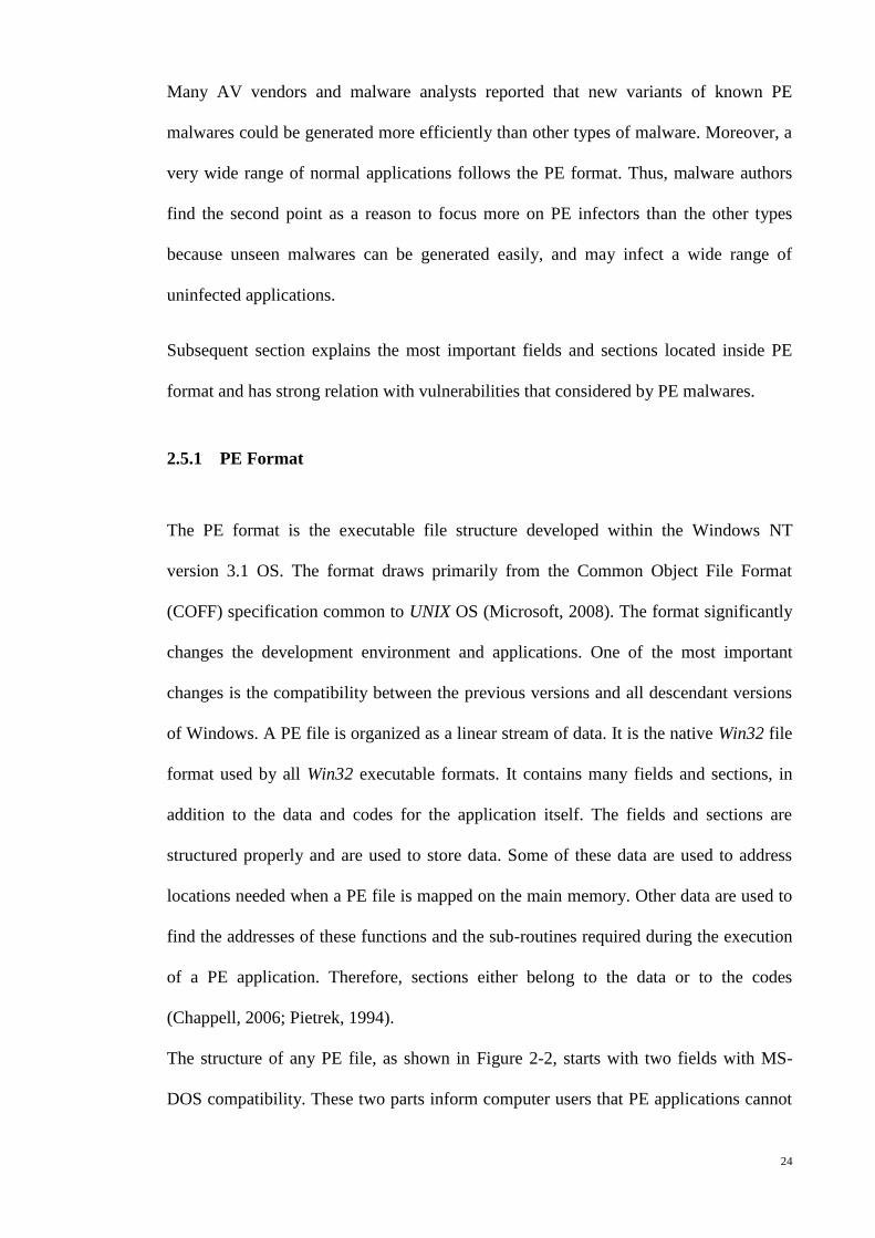
The structure of any PE file, as shown in Figure 2-2, starts with two fields with MS-

DOS compatibility. These two parts inform computer users that PE applications cannot

25

be executed outside MS-DOS. The subsequent parts, which are PE Header, PE

Optional Header, Section Header, and Sections, are associated with PE execution.

The PE Header contains information about the physical layout and properties of the

file, whereas the PE Optional Header contains information about the logical layout of

the PE file. The PE header tells the system how much memory is needed to set aside for

mapping the executable format into the memory.

Figure ‎2-2Format of PE applications (HZV, 2010)

The PE Header file has 20 bytes and seven members. However, malware analysts are

more frequently concerned with only two of the members (Microsoft, 2008, 2011) .

1- NumberOfSection. It gives the number of sections a PE file has. Typically, the

number is nine. However, applications may need more or less sections; thus, the

number changes from one application to another. A malware can then insert a new

section into the victim file and modify the content of this field.

26

2- Characteristics. It contains many flags that point to a specific situation. For

example, a flag is used to identify whether a PE file is executable or is considered

as a DLL.

We move on to the next part, the PE Optional Header. This section comprises 224

bytes. The last 128 bytes contain the DataDirectory. However, the first 96 bytes contain

30 members. Members of the optional header that are closely related to malware

activities are listed below (Y. Choi, Kim, Oh, & Ryou, 2009; Jajodia, 2009).

1- AddressOfEntryPoint. It contains the relative virtual address (RVA) of the first

instruction that is executed when the PE loader is ready to run the PE file.

Malwares usually change this RVA to ensure execution of their codes within the

PE instructions.

2- SectionAlignment. The value in this field adjusts the sections of the PE in the main

memory. It usually creates unused spaces between section offsets.

3- FileAlignment. The value in this field adjusts the PE sections in the file. It also

creates unused spaces between section offsets inside PE files. Malware can use

these slack areas for inserting codes.

4- SizeOfImage. With reference to the SectionAlignment, the value of this field

displays the size of all headers and sections of a PE file inside the main memory.

If a malware needs to increase or decrease the number of sections, the value inside

this field would be modified.

5- SizeOfHeaders. It is the size of all headers in a PE file, such as the DOS header,

PE header, and section table’s header. Malwares need to modify the contents of

these fields to make changes inside any section.

27

6- DataDirectory. It is an array of 16 structures. Each structure is related to an

important data structure in the PE file, such as the import address table that is

responsible for allocating the address of required API functions. Our work focuses

only on two data directories: export and import data directories. These two data

structures are better related to the addresses of API functions that may respond

by/to the subroutines of the PE file during execution.

The following section is on the section header, which is sometimes called the section

table. It contains a number of structures in an array form. The number of structures

should be equal to the number of sections in the section table. Each structure has 12

members. However, only two members are more closely related to malware

behaviours (Basics, 2010).

1- VirtualSize. This field gives the exact size of each section’s data in bytes.

Malwares modify the information in this field to correspond with the

modifications they make.

2- Characteristics. This field explains the status of each section in terms of the ability

to read or write inside the section. It also explains whether the data are initialized

or uninitialized. An important behaviour of malwares is inserting initialized data.

Therefore, monitoring this field indicates monitoring an important behaviour of

malwares.

28

The last part is specified for sections’ contain. Here, the sections contain the main

content of the file, including codes, data, resources, and other executable information.

Each section has a header and a body. The header is stored in the Section Header. The

body, which is the section itself, is not properly structured. However, a linker can still

organise them because the header contains enough information to decipher the content

data (Hamlen et al., 2010; Y. Zhang, Li, Sun, & Qin, 2008).

Typically, an application for Windows NT has nine predefined sections, namely, .text,

.bbs, .rdata, .data, .rsrc, .edata, .idata, .pdata, and .debug. Each section is specific for a

particular function mentioned below (Y. Choi et al., 2009; Hamlen et al., 2010; Jajodia,

2009).

1- .text section. Windows NT keeps all segments of executable codes inside this

section. It is also contains the entry point codes of PE applications. In addition, it

contains the jump thunk table that points to the import address table (IAT), which

facilitates the search for the API functions called by a subroutine.

2- .bss section. Any PE application has uninitialized data, including variables that are

declared as static within a function or source model. This section is used to

represent such data.

3- .rdata section. This area is used to keep recent read-only data.

4- .data section. This section keeps initialized variables and variables used globally

in applications and modules.

5- .rsrc section. This section keeps resource information for a module or application.

6- .edata section. It keeps the Export Directory for an application or DLL. When

present, this section contains information on the names and addresses of exported

functions.

29

7- .idata section. This section contains different information about imported

functions, including the Import Directory and IAT.

8- .debug section. This section contains different information about imported

functions, including the Import Directory and IAT.

Above sections and fields are mostly targeted by PE malwares as vulnerabilities. Next

section gives some explanations on these vulnerabilities.

2.5.2 The Vulnerabilities in PE Format

Permitting malware authors to insert new or modify existing codes and data inside

sections and fields of PE files considered as the simplest vulnerability. A PE is

organized into a linear stream of data. It contains many fields and sections, aside from

the data and codes for the application itself (Szor, 2000). Any PE Explorer software can

exploit the structure of PE applications and then reveal information and data inside each

section and field (Bayer, Kruegel, & Kirda, 2006). Moreover, tools such as text/HEX

editor or WinHex can manually edit the contents of each section and field in a PE

application (Technology, 2010). Therefore, malware authors can easily open and view

the format of any PE application to look for vulnerabilities (Basics, 2010).

The second vulnerability is going back the structure of the PE format itself. It helps a

malware move through the old to the latest versions of the Windows OS because the PE

file format has not changed since its development in Windows NT 3.1. Therefore,

escaping between versions is not difficult for malwares because the above-mentioned

vulnerabilities still remain (Szor, 1998).

Another important vulnerability is the slack and free area that exists in all PE files,

which is attributed to the memory alignment procedure. All PE files use information in

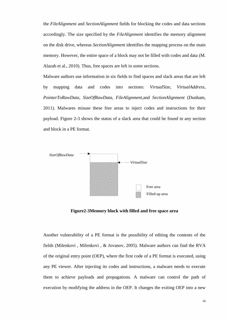
30

the FileAlignment and SectionAlignment fields for blocking the codes and data sections

accordingly. The size specified by the FileAlignment identifies the memory alignment

on the disk drive, whereas SectionAlignment identifies the mapping process on the main

memory. However, the entire space of a block may not be filled with codes and data (M.

Alazab et al., 2010). Thus, free spaces are left in some sections.

Malware authors use information in six fields to find spaces and slack areas that are left

by mapping data and codes into sections: VirtualSize, VirtualAddress,

PointerToRawData, SizeOfRawData, FileAlignment,and SectionAlignment (Dunham,

2011). Malwares misuse these free areas to inject codes and instructions for their

payload. Figure 2-3 shows the status of a slack area that could be found in any section

and block in a PE format.

Figure‎2-3Memory block with filled and free space area

Another vulnerability of a PE format is the possibility of editing the contents of the

fields (Milenkovi , Milenkovi , & Jovanov, 2005). Malware authors can find the RVA

of the original entry point (OEP), where the first code of a PE format is executed, using

any PE viewer. After injecting its codes and instructions, a malware needs to execute

them to achieve payloads and propagations. A malware can control the path of

execution by modifying the address in the OEP. It changes the exiting OEP into a new

Free area

Filled-up area

VirtualSize

SizeOfRawData

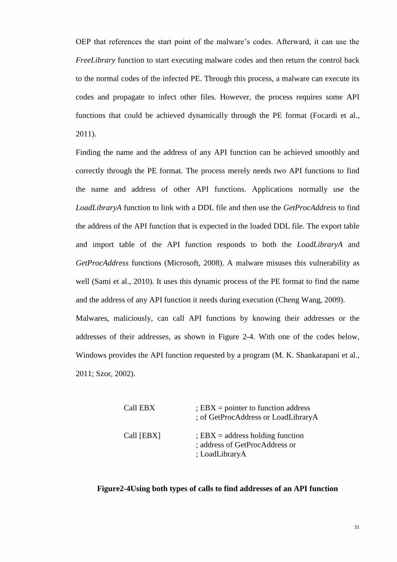
31

OEP that references the start point of the malware’s codes. Afterward, it can use the

FreeLibrary function to start executing malware codes and then return the control back

to the normal codes of the infected PE. Through this process, a malware can execute its

codes and propagate to infect other files. However, the process requires some API

functions that could be achieved dynamically through the PE format (Focardi et al.,

2011).

Finding the name and the address of any API function can be achieved smoothly and

correctly through the PE format. The process merely needs two API functions to find

the name and address of other API functions. Applications normally use the

LoadLibraryA function to link with a DDL file and then use the GetProcAddress to find

the address of the API function that is expected in the loaded DDL file. The export table

and import table of the API function responds to both the LoadLibraryA and

GetProcAddress functions (Microsoft, 2008). A malware misuses this vulnerability as

well (Sami et al., 2010). It uses this dynamic process of the PE format to find the name

and the address of any API function it needs during execution (Cheng Wang, 2009).

Malwares, maliciously, can call API functions by knowing their addresses or the

addresses of their addresses, as shown in Figure 2-4. With one of the codes below,

Windows provides the API function requested by a program (M. K. Shankarapani et al.,

2011; Szor, 2002).

Call EBX ; EBX = pointer to function address

; of GetProcAddress or LoadLibraryA

Call [EBX] ; EBX = address holding function

; address of GetProcAddress or

; LoadLibraryA

Figure‎2-4Using both types of calls to find addresses of an API function

32

New malicious API calls by malwares always used whenever malware authors discover

new vulnerability / ies inside the structure of the PE. On the other side, malware

detection researchers also perform studies on such formats to trace the fingerprints of

malicious API calls of new PE malware (Szor, 2006).The next section shows the

purposes that a PE malware makes malicious API calls for.

2.6 Abusing API Function Behaviours of PE Malwares

As mentioned in section 2.3, PE malwares can affect OS integrity. They gain this

capability after successfully infecting executable files (Solomon, 1993). Through PE

format infection, a PE malware can exploit OS vulnerabilities and then insert codes into

some parts of the OS. Then, they can abuse system resources to infect more files (Essam

Al Daoud, 2008).

The infection of executable formats allows PE malwares to take over OS resources

easily and then use these resources as normal applications (Bo-yun Zhang, 2006). One

of the most important resources a PE malware uses is the API function. A PE malware

needs to call such system functions to execute its functionalities smoothly and normally

inside the Windows OS (S. Choi et al., 2007). As illustrated in Figure 2-4, a malware

can easily find the address of a system call that needs through execution (M. Alazab et

al., 2010).

A malware can call an API function in the same way that a normal application does.

However, it has a different purpose for such a call. A malware differs from a normal

application in calling an API function in that the malware abuses these functions to

perform payloads and to propagate (Bai et al., 2009). Therefore, during malware system

calling, malware analysts see some behaviours that are not frequently seen during the

system calls of normal applications (M Alazab et al., 2010). .

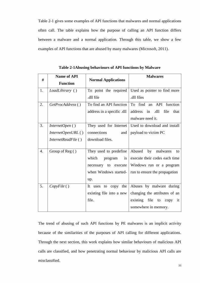
33

Table 2-1 gives some examples of API functions that malwares and normal applications

often call. The table explains how the purpose of calling an API function differs

between a malware and a normal application. Through this table, we show a few

examples of API functions that are abused by many malwares (Microsoft, 2011).

Table ‎2-1Abusing behaviours of API functions by Malware

# Name of API

Function Normal Applications

Malwares

1. LoadLibirary ( ) To point the required

.dll file

Used as pointer to find more

.dll files

2. GetProcAddress ( ) To find an API function

address in a specific .dll

To find an API function

address in .dll file that

malware need it.

3. InternetOpen ( )

InternetOpenURL ( )

InternetReadFile ( )

They used for Internet

connections and

download files.

Used to download and install

payload to victim PC

4. Group of Reg ( ) They used to predefine

which program is

necessary to execute

when Windows started-

up.

Abused by malwares to

execute their codes each time

Windows run or a program

run to ensure the propagation

5. CopyFile ( ) It uses to copy the

existing file into a new

file.

Abuses by malware during

changing the attributes of an

existing file to copy it

somewhere in memory.

The trend of abusing of such API functions by PE malwares is an implicit activity

because of the similarities of the purposes of API calling for different applications.

Through the next section, this work explains how similar behaviours of malicious API

calls are classified, and how penetrating normal behaviour by malicious API calls are

misclassified.

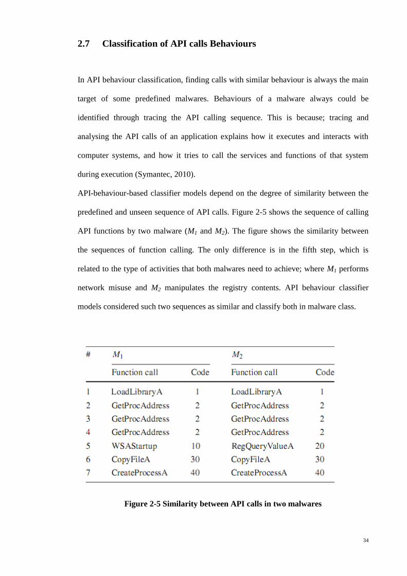
34

2.7 Classification of API calls Behaviours

In API behaviour classification, finding calls with similar behaviour is always the main

target of some predefined malwares. Behaviours of a malware always could be

identified through tracing the API calling sequence. This is because; tracing and

analysing the API calls of an application explains how it executes and interacts with

computer systems, and how it tries to call the services and functions of that system

during execution (Symantec, 2010).

API-behaviour-based classifier models depend on the degree of similarity between the

predefined and unseen sequence of API calls. Figure 2-5 shows the sequence of calling

API functions by two malware (M1 and M2). The figure shows the similarity between

the sequences of function calling. The only difference is in the fifth step, which is

related to the type of activities that both malwares need to achieve; where M1 performs

network misuse and M2 manipulates the registry contents. API behaviour classifier

models considered such two sequences as similar and classify both in malware class.

Figure ‎2-5 Similarity between API calls in two malwares

35

Like the API functions of Figure 2-5, malwares can misuse many other API functions.

For instant, the API function CreateWindowExA misused by malwares to build a

message and present it to user ones it has executed (Dunham, 2011). Other functions

misused for other activities. For example, below functions may use by malwares to

control HTTP communication: “HttpSendRequestExA, HttpQueryInfoA ,

HttpSendRequestExW , InternetQueryDataAvailable , InternetReadFileExA ,

HttpSendRequestW, GetUrlCachEntryInfoW”(Szor, 2000). Such calls supposedly show

abnormalities as malwares misuse them for different malicious behaviours. However,

some parts of this sequence remain similar to normal behaviours.

As shown in Figure 2-5, the first four calls that are used by both malwares are often

found in the API sequence of normal applications. Malwares and normal applications

often use these four API functions to acquire information about functions that form the

OS. As a second example, a system call sequence can have the following form:

“OpenRegistry, ManipulateRegistry, OpenSocket, WriteSocket, ...”; this form can

characterize malicious calls that manipulate the Windows registry database and then

transmit information through network socket operations (Xiao & Stibor, 2011). Some

other malwares misuse API function by inserting their malicious calls in the path of

normal calls. For instant, if the GetDate function is in the sub-sequence of the

CreateFile, then the name of the file depends on the data and varies from data set to

another (Bayer, Comparetti, et al., 2009). Although, malware analysts consider such

behaviour as a malicious call because normal applications do not need to do these

procedures, malicious classifier models cannot distinguish them accurately.

36

There are many calls that made by malwares; however, a normal program may do the

same calling sequences too. Many functions are used properly by a normal application

for a privileged activity while they misused by a malware for non-privileged issues

(Table 2-1). Furthermore, the way that both types of application call systems and the

ways the system responds bring both normal and malware system-calling behaviours

close to each other.

This level of similarity makes distinguishing the normal calls from the malicious calls

difficult for classifier models. Therefore, many classifier models either misclassify

unseen calls or doubtfully classify them into a class. Both situations negatively affect

the accuracy of the classifier model.

Next section presents many methods that proposed by researchers as malicious API call

classifier models to distinguish malicious calls in PE malwares.

2.8 Review on Malicious API calls Classifier Models

Although the concept of API tracing goes back to 1996, researchers proposed active

efforts on this topic only after 2005 (Omer, 2009). Moreover, the idea of infecting

executable files goes back to December 1986. At the time, Ralf Burger, who is the

creator of the Virdem, presented a model of programs that could replicate themselves

by adding their codes to executable DOS files in .COM format (Solomon, 1993). The

codes that presented by Burger were considered the first MS-DOS executable infectors.

However, the first Win32 (Windows 95 and Windows NT) infector goes back to 1996,

when a few viruses penetrated Windows 95 through the PE format. For instance, a

Win32 virus called “Win95.Punch” that could infect the .EXE format and stay in the

memory as a VxD driver was discovered. Similarly, the virus BOZA, created by some

37

Australian Virus Laboratory and Distribution (VLAD) group, appeared the same year

Windows 95 was introduced (Fu et al., 2008; Szor, 1998).

After that, the PE infectors or Win32 viruses developed gradually. However, until 2000,

the field of PE or Win32 viruses was still in its early stage, as mentioned in (Szor,

1998). The most important problem found at that time was the compatibility of

Windows 95 that kept most DOS-based viruses compatible with the new Widows 95,

such as the Yankee-Doodle (Szor, 2000). Based on our best knowledge the first article

that covers PE infectors, the techniques used to penetrate Windows OS and some

detection strategies were conducted in 1998 (Szor, 1998). The author published a new

version of his article in (Szor, 2000). The author succeeded to describe the format of the

PE files and the locations that the viruses most possibly changed or modified.

Moreover, he explained how computer viruses abused the Win32 API in Windows 95.

He mentioned the necessity of working with some behaviour-based techniques to detect

PE infectors.

At present, different detection models depend on disparate methods and techniques to

detect PE malwares (Xiang, Hao, Zhang, & Liu, 2008). However, detection models

operate as knowledge-based, statistical-based, or machine-learning-based systems (Szor,

2006). The independent parameters of any detection models are changed, depending on

their types. For instance, the knowledge-based detection system, also known as the

signature-based detection system, depends on some predefined strings inside a

suspected file. Meanwhile, statistical- and machine-learning-based systems frequently

use other parameters, such as API call tracing or instructions and redundant code

monitoring (Essam Al Daoud, 2008). Moreover, all detection models are either static-

based or dynamic-based systems. Static detection models check suspected files and

applications without executing them. However, dynamic execution models scan the

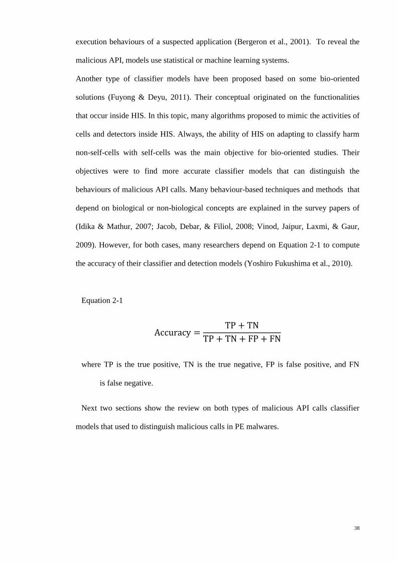
38

execution behaviours of a suspected application (Bergeron et al., 2001). To reveal the

malicious API, models use statistical or machine learning systems.

Another type of classifier models have been proposed based on some bio-oriented

solutions (Fuyong & Deyu, 2011). Their conceptual originated on the functionalities

that occur inside HIS. In this topic, many algorithms proposed to mimic the activities of

cells and detectors inside HIS. Always, the ability of HIS on adapting to classify harm

non-self-cells with self-cells was the main objective for bio-oriented studies. Their

objectives were to find more accurate classifier models that can distinguish the

behaviours of malicious API calls. Many behaviour-based techniques and methods that

depend on biological or non-biological concepts are explained in the survey papers of

(Idika & Mathur, 2007; Jacob, Debar, & Filiol, 2008; Vinod, Jaipur, Laxmi, & Gaur,

2009). However, for both cases, many researchers depend on Equation 2-1 to compute

the accuracy of their classifier and detection models (Yoshiro Fukushima et al., 2010).

Equation 2-1

where TP is the true positive, TN is the true negative, FP is false positive, and FN

is false negative.

Next two sections show the review on both types of malicious API calls classifier

models that used to distinguish malicious calls in PE malwares.

39

2.8.1 Non-Biological API Detection Models

Detection systems that depend on statistical and machine learning algorithms or

methods may be considered as non-biological models. They use techniques, such as

data mining, conditional probability, the Naive Bayes theory, neural network, fuzzy

logic, and other machine learning techniques. Researchers use disparate non-biological

models in recent years to propose detection systems. In 2001, a non-biological model

was proposed in (Schultz, Eskin, Zadok, & Stolfo, 2001) to reveal malicious executable

files. These models depend on the frequency calculation of API functions that are called

by benign and malware applications. They use the frequency figures to find features for

their mining systems. They train their system on the known features of malware. Data

mining techniques are used to detect unseen malwares, whereas the Naive Bayes

method is used to classify the suspected executable file.

Another non-biological model, the heuristic technique, was used by (Szor, 2002) by

executing a suspected application in a virtual machine. To develop this heuristic model,

the author referred to his article (Szor, 2000), explaining most sections and fields in a

PE file whose contents the malware might modify. The study monitored the API calls

used by normal applications or abused by three types of malware during memory

access. The author evaluated the monitored API to reveal malicious executable.

A static model was proposed by (Bergeron et al., 2001) to reveal executable codes.

Authors in this work represent an API call or a block of API calls as an intermediate

form. The authors showed the direction of the flow between these intermediate blocks.

Finally, the work extracted a control flow compared with many security policies to

reveal malicious executable codes.

40

When malwares penetrate systems, they inject malicious codes, dynamically generate

malicious codes, or perform obfuscated malicious codes (Xiang et al., 2008). These

behaviours could be revealed by tracing and monitoring the API calls of a suspected PE

file, as was conducted in a study proposed by (Rabek, Khazan, Lewandowski, &

Cunningham, 2003). Another powerful method used by different malwares is the

polymorphic technique. This technique gives malware the ability to change signatures

and to rearrange codes (Szor, 2006). Therefore, signature-based detection systems

cannot overcome such malwares. More time and effort are required to analyse

polymorphic malwares as they become more complex. By controlling API functions

and system calls, such techniques could be revealed, as proposed by (J-Y. Xu, 2004). In

the aforementioned work, the similarity was measured between the original virus and

the variants that were generated through polymorphic techniques. A threshold value was

defined to evaluate the degree of similarity between two API call sequences. Thus, the

degree of similarity between two API sequences could be obtained, and accordingly, the

two most similar sequences could be identified.

Different behaviours of malware, including mass mailing and registry overwriting, were

used by (Mori, 2004) to define malicious codes. They defined these behaviours on the

level of Win32 API calls. Static code analysis and dynamic code simulation were

combined to identify these behaviours. The authors argued that different types of mail

malware could be detected by tracing Win32 API calls through their respective

proposed approach.

To analyse malware behaviours, malware analysts rely on manual steps. An approach

was proposed by (Bayer et al., 2006) to analyse malware dynamically by increasing the

number of malwares. Their proposed work found similar dynamic behaviours for

malware based on certain predefined policies. During their implementation, they

depended on tracing the Win32 API calls, as in the previous studies.

41

One of the most important behaviours of malware is propagation among files within the

same host or propagation over networks (C. W. J. P. R. Zhao & Liu, 2009). A model

was proposed by (Y. Ye, Wang, Li, & Ye, 2007) to implement malware detection based

on propagation behaviour. In this work, the authors relied on data mining to develop a

model by using an objective-oriented association mining-based classification. Through

this approach, vectors of Win32 API calls could be monitored to detect malwares.

Malwares can locate each address of required API functions via different means. For

instance, the Boza virus uses hard-coded addresses, whereas Win32.Bozano uses

homonymy functions. However, most malwares, such as Win32.Aztec, use a string

array to store the name and address of API calls. Consequently, researchers (Fu et al.,

2008) proposed an approach for extracting API calls in suspected files. Some indirect

API calls made by many malwares could not be revealed easily. This issue was solved

by comparing the original API call sequences and the indirect API call policies used by

the malwares.

Considering that the number of malicious codes approximately equals the number of

normal codes (Shabtai, Moskovitch, Elovici, & Glezer, 2009), additional studies were

conducted from 2008 through 2012 to detect malicious API calls. Table 2-2 mentions

most of these studies.

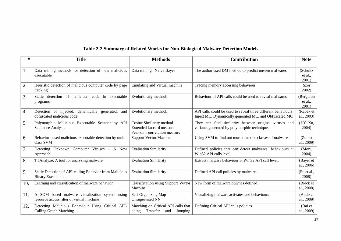
42

Table ‎2-2 Summary of Related Works for Non-Biological Malware Detection Models

# Title Methods Contribution Note

1. Data mining methods for detection of new malicious

executable

Data mining , Naive Bayes The author used DM method to predict unseen malwares (Schultz

et al.,

2001)

2. Heuristic detection of malicious computer code by page

tracking

Emulating and Virtual machine Tracing memory accessing behaviour (Szor,

2002)

3. Static detection of malicious code in executable

programs

Evolutionary methods. Behaviour of API calls could be used to reveal malwares (Bergeron

et al.,

2001)

4. Detection of injected, dynamically generated, and

obfuscated malicious code

Evolutionary method. API calls could be used to reveal three different behaviours;

Inject MC, Dynamically generated MC, and Obfuscated MC

(Rabek et

al., 2003)

5. Polymorphic Malicious Executable Scanner by API

Sequence Analysis

Cosine Similarity method.

Extended Jaccard measure.

Pearson’s correlation measure

They can find similarity between original viruses and

variants generated by polymorphic technique.

(J-Y. Xu,

2004)

6. Behavior-based malicious executable detection by multi-

class SVM

Support Vector Machine Using SVM to find out more than one classes of malwares (Zou et

al., 2009)

7. Detecting Unknown Computer Viruses – A New

Approach

Evaluation Similarity Defined policies that can detect malwares’ behaviours at

Win32 API calls level.

(Mori,

2004)

8. TTAnalyze: A tool for analyzing malware Evaluation Similarity Extract malware behaviour at Win32 API call level. (Bayer et

al., 2006)

9. Static Detection of API-calling Behavior from Malicious

Binary Executable

Evaluation Similarity Defined API call policies by malwares (Fu et al.,

2008)

10. Learning and classification of malware behavior

Classification using Support Vector

Machine

New form of malware policies defined. (Rieck et

al., 2008)

11. A SOM based malware visualization system using

resource access filter of virtual machine

Self-Organizing Map

Unsupervised NN

Visualizing malware activates and behaviours (Ando et

al., 2009)

12. Detecting Malicious Behaviour Using Critical API-

Calling Graph Matching

Matching on Critical API calls that

doing Transfer and Jumping

Defining Critical API calls policies. (Bai et

al., 2009)

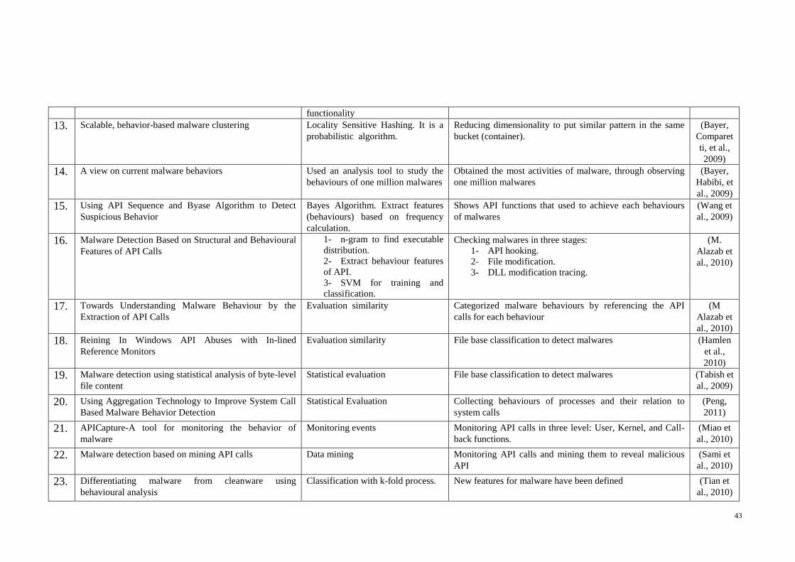
https://www.auto.tuwien.ac.at/~chris/research/doc/eicar06_ttanalyze.pdf

http://www.springerlink.com/index/Q87P5407J3201267.pdf

43

functionality

13. Scalable, behavior-based malware clustering Locality Sensitive Hashing. It is a

probabilistic algorithm.

Reducing dimensionality to put similar pattern in the same

bucket (container).

(Bayer,

Comparet

ti, et al.,

2009)

14. A view on current malware behaviors Used an analysis tool to study the

behaviours of one million malwares

Obtained the most activities of malware, through observing

one million malwares

(Bayer,

Habibi, et

al., 2009)

15. Using API Sequence and Byase Algorithm to Detect

Suspicious Behavior

Bayes Algorithm. Extract features

(behaviours) based on frequency

calculation.

Shows API functions that used to achieve each behaviours

of malwares

(Wang et

al., 2009)

16. Malware Detection Based on Structural and Behavioural

Features of API Calls

1- n-gram to find executable

distribution.

2- Extract behaviour features

of API.

3- SVM for training and

classification.

Checking malwares in three stages:

1- API hooking.

2- File modification.

3- DLL modification tracing.

(M.

Alazab et

al., 2010)

17. Towards Understanding Malware Behaviour by the

Extraction of API Calls

Evaluation similarity Categorized malware behaviours by referencing the API

calls for each behaviour

(M

Alazab et

al., 2010)

18. Reining In Windows API Abuses with In-lined

Reference Monitors

Evaluation similarity File base classification to detect malwares (Hamlen

et al.,

2010)

19. Malware detection using statistical analysis of byte-level

file content

Statistical evaluation File base classification to detect malwares (Tabish et

al., 2009)

20. Using Aggregation Technology to Improve System Call

Based Malware Behavior Detection

Statistical Evaluation Collecting behaviours of processes and their relation to

system calls

(Peng,

2011)

21. APICapture-A tool for monitoring the behavior of

malware

Monitoring events Monitoring API calls in three level: User, Kernel, and Call-

back functions.

(Miao et

al., 2010)

22. Malware detection based on mining API calls Data mining Monitoring API calls and mining them to reveal malicious

API

(Sami et

al., 2010)

23. Differentiating malware from cleanware using

behavioural analysis

Classification with k-fold process. New features for malware have been defined (Tian et

al., 2010)

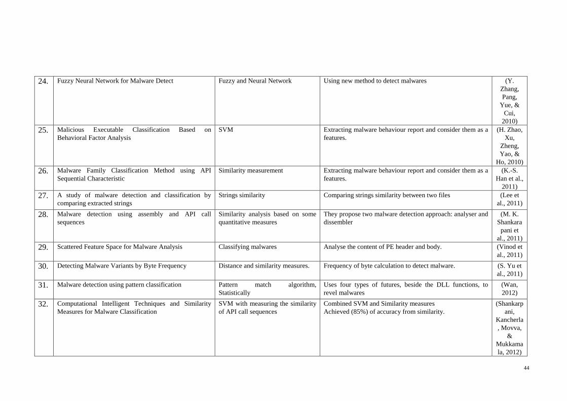
44

24. Fuzzy Neural Network for Malware Detect Fuzzy and Neural Network Using new method to detect malwares (Y.

Zhang,

Pang,

Yue, &

Cui,

2010)

25. Malicious Executable Classification Based on

Behavioral Factor Analysis

SVM Extracting malware behaviour report and consider them as a

features.

(H. Zhao,

Xu,

Zheng,

Yao, &

Ho, 2010)

26. Malware Family Classification Method using API

Sequential Characteristic

Similarity measurement Extracting malware behaviour report and consider them as a

features.

(K.-S.

Han et al.,

2011)

27. A study of malware detection and classification by

comparing extracted strings

Strings similarity Comparing strings similarity between two files (Lee et

al., 2011)

28. Malware detection using assembly and API call

sequences

Similarity analysis based on some

quantitative measures

They propose two malware detection approach: analyser and

dissembler

(M. K.

Shankara

pani et

al., 2011)

29. Scattered Feature Space for Malware Analysis Classifying malwares Analyse the content of PE header and body. (Vinod et

al., 2011)

30. Detecting Malware Variants by Byte Frequency Distance and similarity measures. Frequency of byte calculation to detect malware. (S. Yu et

al., 2011)

31. Malware detection using pattern classification Pattern match algorithm,

Statistically

Uses four types of futures, beside the DLL functions, to

revel malwares

(Wan,

2012)

32. Computational Intelligent Techniques and Similarity

Measures for Malware Classification

SVM with measuring the similarity

of API call sequences

Combined SVM and Similarity measures

Achieved (85%) of accuracy from similarity.

(Shankarp

ani,

Kancherla

, Movva,

&

Mukkama

la, 2012)

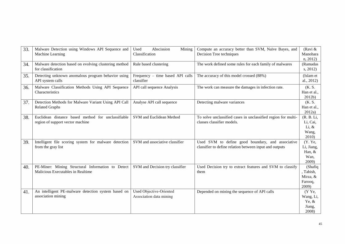
45

33. Malware Detection using Windows API Sequence and

Machine Learning

Used Abscission Mining

Classification

Compute an accuracy better than SVM, Naïve Bayes, and

Decision Tree techniques

(Ravi &

Manohara

n, 2012)

34. Malware detection based on evolving clustering method

for classification

Rule based clustering The work defined some rules for each family of malwares (Ramadas

s, 2012)

35. Detecting unknown anomalous program behavior using

API system calls

Frequency – time based API calls

classifier

The accuracy of this model crossed (88%) (Islam et

al., 2012)

36. Malware Classification Methods Using API Sequence

Characteristics

API call sequence Analysis The work can measure the damages in infection rate. (K. S.

Han et al.,

2012b)

37. Detection Methods for Malware Variant Using API Call

Related Graphs

Analyse API call sequence Detecting malware variances (K. S.

Han et al.,

2012a)

38. Euclidean distance based method for unclassifiable

region of support vector machine

SVM and Euclidean Method To solve unclassified cases in unclassified region for multi-

classes classifier models.

(R. B. Li,

Li, Cai,

Li, &

Wang,

2010)

39. Intelligent file scoring system for malware detection

from the gray list

SVM and associative classifier Used SVM to define good boundary, and associative

classifier to define relation between input and outputs

(Y. Ye,

Li, Jiang,

Han, &

Wan,

2009)

40. PE-Miner: Mining Structural Information to Detect

Malicious Executables in Realtime

SVM and Decision try classifier Used Decision try to extract features and SVM to classify

them

(Shafiq

, Tabish,

Mirza, &

Farooq,

2009)

41. An intelligent PE-malware detection system based on

association mining

Used Objective-Oriented

Association data mining

Depended on mining the sequence of API calls (Y Ye,

Wang, Li,

Ye, &

Jiang,

2008)

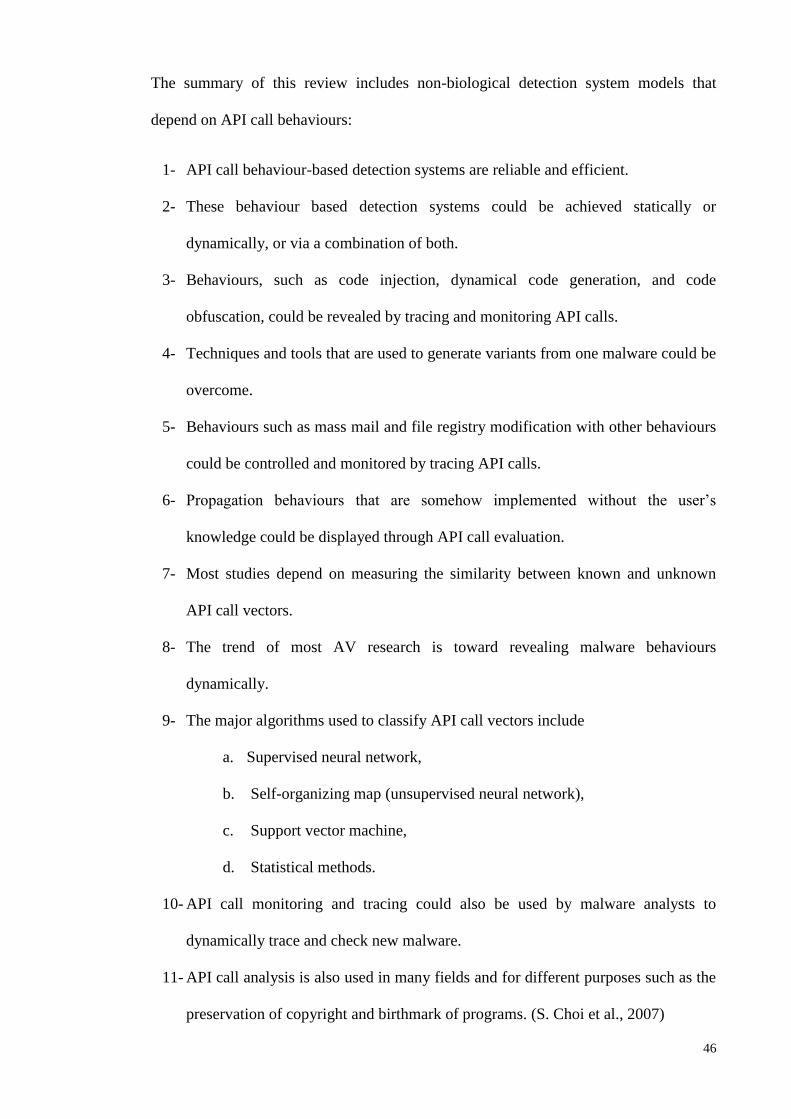
46

The summary of this review includes non-biological detection system models that

depend on API call behaviours:

1- API call behaviour-based detection systems are reliable and efficient.

2- These behaviour based detection systems could be achieved statically or

dynamically, or via a combination of both.

3- Behaviours, such as code injection, dynamical code generation, and code

obfuscation, could be revealed by tracing and monitoring API calls.

4- Techniques and tools that are used to generate variants from one malware could be

overcome.

5- Behaviours such as mass mail and file registry modification with other behaviours

could be controlled and monitored by tracing API calls.

6- Propagation behaviours that are somehow implemented without the user’s

knowledge could be displayed through API call evaluation.

7- Most studies depend on measuring the similarity between known and unknown

API call vectors.

8- The trend of most AV research is toward revealing malware behaviours

dynamically.

9- The major algorithms used to classify API call vectors include

a. Supervised neural network,

b. Self-organizing map (unsupervised neural network),

c. Support vector machine,

d. Statistical methods.

10- API call monitoring and tracing could also be used by malware analysts to

dynamically trace and check new malware.

11- API call analysis is also used in many fields and for different purposes such as the

preservation of copyright and birthmark of programs. (S. Choi et al., 2007)

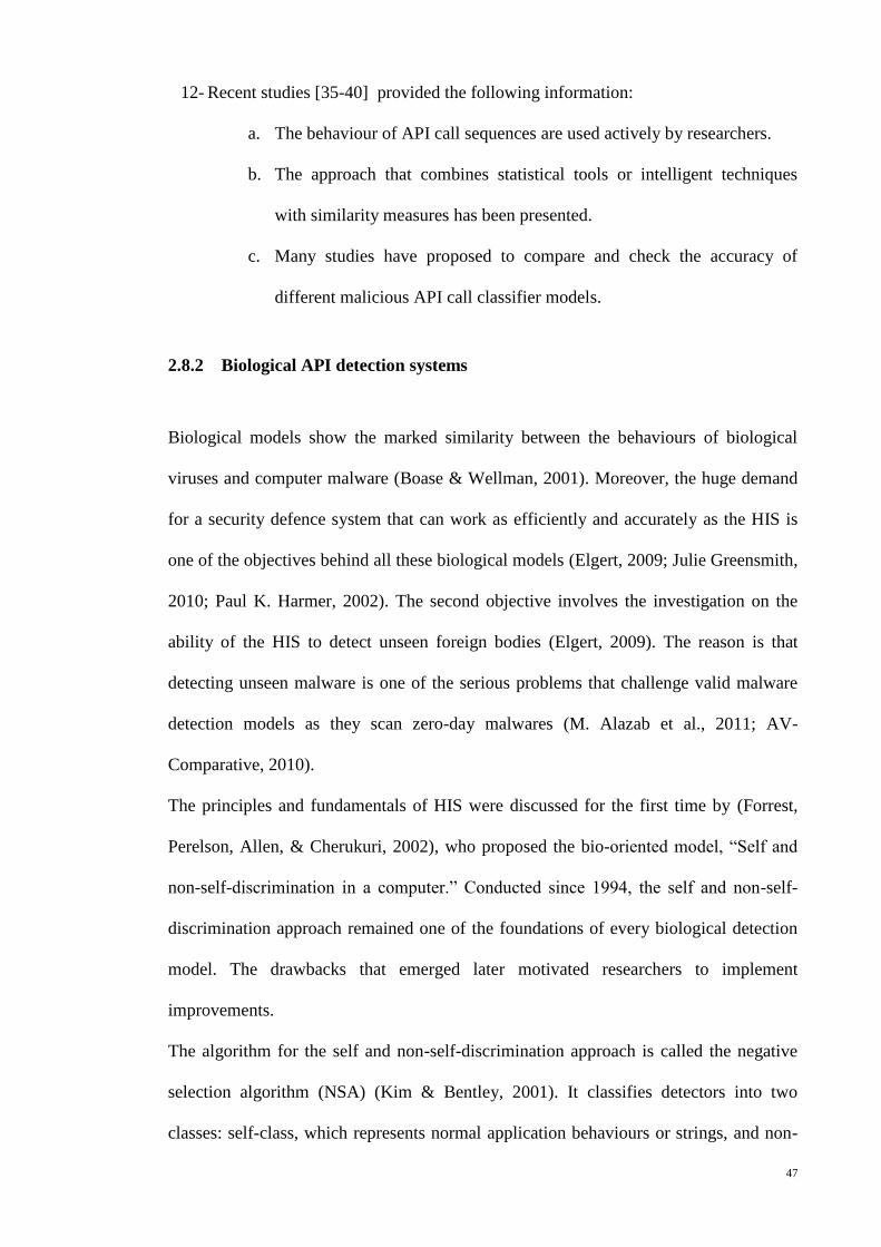
47

12- Recent studies [35-40] provided the following information:

a. The behaviour of API call sequences are used actively by researchers.

b. The approach that combines statistical tools or intelligent techniques

with similarity measures has been presented.

c. Many studies have proposed to compare and check the accuracy of

different malicious API call classifier models.

2.8.2 Biological API detection systems

Biological models show the marked similarity between the behaviours of biological

viruses and computer malware (Boase & Wellman, 2001). Moreover, the huge demand

for a security defence system that can work as efficiently and accurately as the HIS is

one of the objectives behind all these biological models (Elgert, 2009; Julie Greensmith,

2010; Paul K. Harmer, 2002). The second objective involves the investigation on the

ability of the HIS to detect unseen foreign bodies (Elgert, 2009). The reason is that

detecting unseen malware is one of the serious problems that challenge valid malware

detection models as they scan zero-day malwares (M. Alazab et al., 2011; AV-

Comparative, 2010).

The principles and fundamentals of HIS were discussed for the first time by (Forrest,

Perelson, Allen, & Cherukuri, 2002), who proposed the bio-oriented model, “Self and

non-self-discrimination in a computer.” Conducted since 1994, the self and non-self-

discrimination approach remained one of the foundations of every biological detection

model. The drawbacks that emerged later motivated researchers to implement

improvements.

The algorithm for the self and non-self-discrimination approach is called the negative

selection algorithm (NSA) (Kim & Bentley, 2001). It classifies detectors into two

classes: self-class, which represents normal application behaviours or strings, and non-

48

self, which represents malware behaviours. The implementation of the NSA algorithm

proceeds as follows: an unknown string or behaviour that does not match any detector

inside the self-class could be considered as a detector inside the non-self-class (Kim &

Bentley, 2001).

A number of researchers (Fuyong & Deyu, 2011; Ji & Dasgupta, 2009; Shen, Wen-Jian,

& Xu-Fa, 2007; Tao, Shiguang, & Dejiao, 2010; Yang, Deng, Chen, & Wang, 2011)

proved that not every unknown string or behaviour could be considered as non-self.

This issue was noted as a main drawback for the NSA; it encouraged researchers to

work on this aspect to improve the algorithm (Fuyong & Deyu, 2011; Kim & Bentley,

2001; P. T. Zhang, Wang, & Tan, 2010).

The clonal selection algorithm (CSA) was one of the alternative algorithms to NSA that

was proposed to build detection or classification models (Khaled et al., 2010;

Xiangrong Zhang 2004; Y. Yu & Hou, 2004; Zuben, 2001). In using the CSA, classes

are divided into two main classes: self-detectors and non-self-detectors. Unlike the case

in NSA, maturation in CSA is performed among non-self-detectors to generate unseen

non-self-detectors. The new non-self-detectors are then compared with the known self-

detectors. If a match is found during the comparison, the newly generated non-self-

detector is cancelled. Otherwise, the non-self-detector is considered a member of the

non-self-detector class (Zuben, 2001). The CSA can effectively detect variants of old

viruses and malwares because the CSA process generates new variants of detectors from

old detectors. One of the drawbacks of the CSA is its weak diversity that is due to the

maturation inside the same domain of non-self-detectors, which also causes global

optimization problems (Yidan Luo & Jiang, 2008).

Another alternative to NSA is the danger theory (U Aickelin & Cayzer, 2002). Similar

to the self and non-self-approaches, the danger theory supports the classification

process. In this theory, the HIS responds only to danger cases among numerous foreign

49

cases found. A non-self-behaviour does not have to be classified as malware. Detection

models should be able to distinguish between a dangerous, hostile, or unfriendly non-

self-behaviour(U. Aickelin, Bentley, Cayzer, Kim, & McLeod, 2003; Kim, Greensmith,

Twycross, & Aickelin, 2005). The danger theory increases the efficiency of detection

models because it minimizes the dimensions of the domain. However, measuring the

degree of danger for any non-self-application is not easy.

The identification of a threshold to discriminate between dangerous and friendly non-

self-cases is difficult. In such a situation, classification models put many cases in a

doubtful position (Manzoor, Shafiq, Tabish, & Farooq, 2009).

To identify more alternatives to NSA and CSA, researchers investigated the

functionalities of all parts of HIS and then examined the phenomenon that occurs within

HIS. As a result, an AIS algorithm was proposed (D Dasgupta, 2007; D. Dasgupta, Yu,

& Nino, 2010; De Castro & Timmis, 2002; He, Yiwen, Tao, & Ting, 2010; S. Hofmeyr

& Forrest, 1999; Khaled et al., 2010; Paul K. Harmer, 2002)]. HIS contains different

activities and functionalities. Parts of HIS may achieve one or more functions as the

entire system defends the human body. Some functionalities may be implemented as a

form of a distributed system, whereas others are achieved in the form of a centralized

system (D Dasgupta, 2007; Jieqiong Zheng 2010; Paul K. Harmer, 2002). The ability to

adapt the valid detectors to match unseen harmful foreign bodies without any false

alarm is the key to the success of HIS (Health, 2003) and is the goal of most biological

models.

Several functionalities of HIS mentioned in (Paul K. Harmer, 2002) could be proposed

for computer security applications. Table 2-3 summarizes the functionalities and

activities proposed in various detection models:

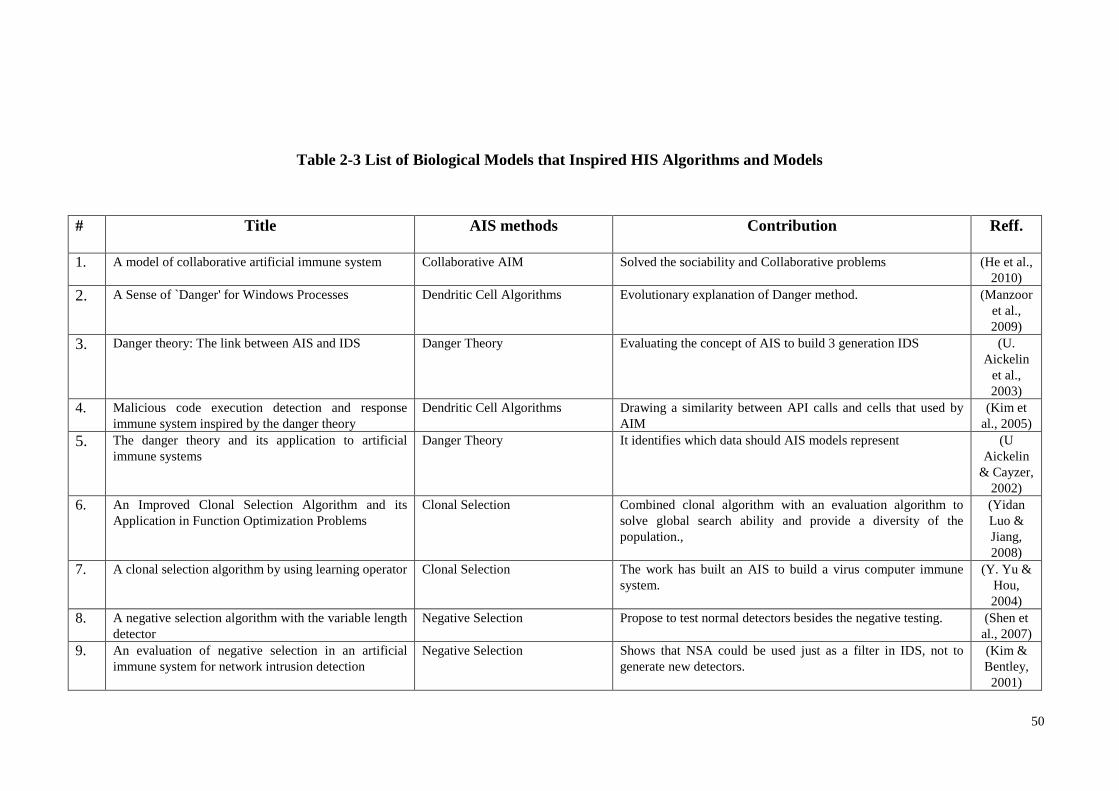
50

Table ‎2-3 List of Biological Models that Inspired HIS Algorithms and Models

# Title AIS methods Contribution Reff.

1. A model of collaborative artificial immune system Collaborative AIM Solved the sociability and Collaborative problems (He et al.,

2010)

2. A Sense of `Danger' for Windows Processes Dendritic Cell Algorithms Evolutionary explanation of Danger method. (Manzoor

et al.,

2009)

3. Danger theory: The link between AIS and IDS Danger Theory Evaluating the concept of AIS to build 3 generation IDS (U.

Aickelin

et al.,

2003)

4. Malicious code execution detection and response

immune system inspired by the danger theory

Dendritic Cell Algorithms Drawing a similarity between API calls and cells that used by

AIM

(Kim et

al., 2005)

5. The danger theory and its application to artificial

immune systems

Danger Theory It identifies which data should AIS models represent (U

Aickelin

& Cayzer,

2002)

6. An Improved Clonal Selection Algorithm and its

Application in Function Optimization Problems

Clonal Selection Combined clonal algorithm with an evaluation algorithm to

solve global search ability and provide a diversity of the

population.,

(Yidan

Luo &

Jiang,

2008)

7. A clonal selection algorithm by using learning operator Clonal Selection The work has built an AIS to build a virus computer immune

system.

(Y. Yu &

Hou,

2004)

8. A negative selection algorithm with the variable length

detector

Negative Selection Propose to test normal detectors besides the negative testing. (Shen et

al., 2007)

9. An evaluation of negative selection in an artificial

immune system for network intrusion detection

Negative Selection Shows that NSA could be used just as a filter in IDS, not to

generate new detectors.

(Kim &

Bentley,

2001)

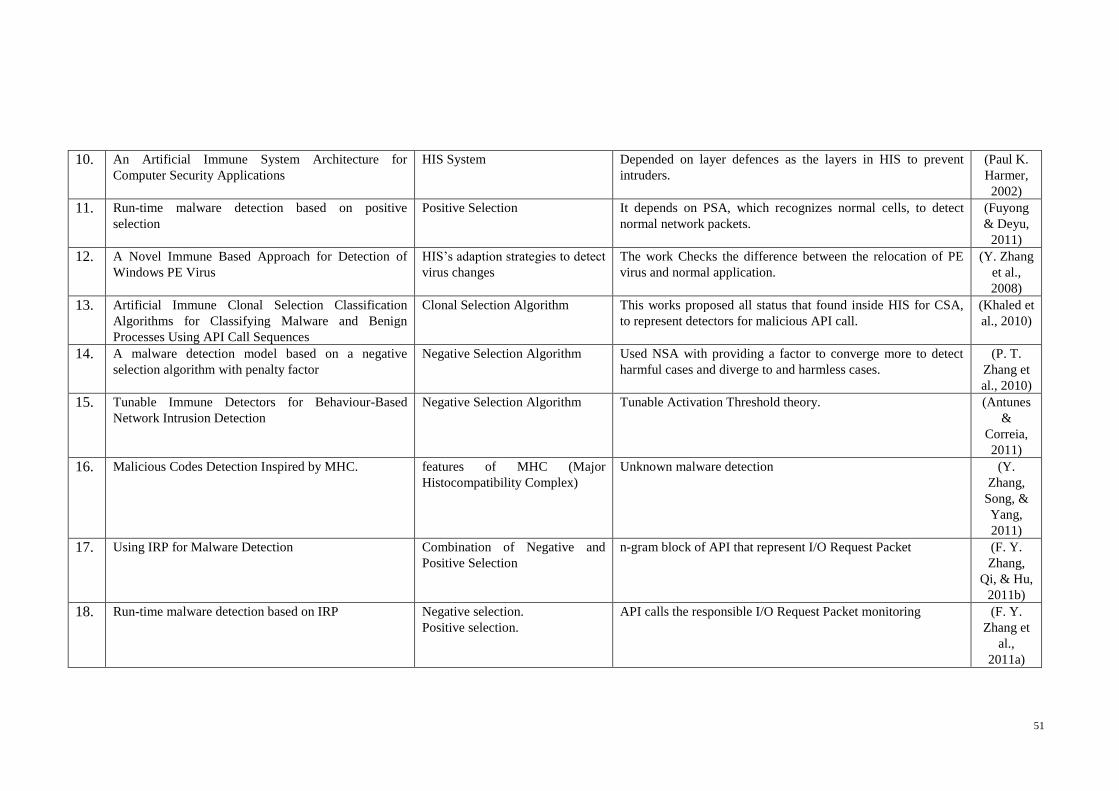
51

10. An Artificial Immune System Architecture for

Computer Security Applications

HIS System Depended on layer defences as the layers in HIS to prevent

intruders.

(Paul K.

Harmer,

2002)

11. Run-time malware detection based on positive

selection

Positive Selection It depends on PSA, which recognizes normal cells, to detect

normal network packets.

(Fuyong

& Deyu,

2011)

12. A Novel Immune Based Approach for Detection of

Windows PE Virus

HIS’s adaption strategies to detect

virus changes

The work Checks the difference between the relocation of PE

virus and normal application.

(Y. Zhang

et al.,

2008)

13. Artificial Immune Clonal Selection Classification

Algorithms for Classifying Malware and Benign

Processes Using API Call Sequences

Clonal Selection Algorithm This works proposed all status that found inside HIS for CSA,

to represent detectors for malicious API call.

(Khaled et

al., 2010)

14. A malware detection model based on a negative

selection algorithm with penalty factor

Negative Selection Algorithm Used NSA with providing a factor to converge more to detect

harmful cases and diverge to and harmless cases.

(P. T.

Zhang et

al., 2010)

15. Tunable Immune Detectors for Behaviour-Based

Network Intrusion Detection

Negative Selection Algorithm Tunable Activation Threshold theory. (Antunes

&

Correia,

2011)

16. Malicious Codes Detection Inspired by MHC. features of MHC (Major

Histocompatibility Complex)

Unknown malware detection (Y.

Zhang,

Song, &

Yang,

2011)

17. Using IRP for Malware Detection Combination of Negative and

Positive Selection

n-gram block of API that represent I/O Request Packet (F. Y.

Zhang,

Qi, & Hu,

2011b)

18. Run-time malware detection based on IRP Negative selection.

Positive selection.

API calls the responsible I/O Request Packet monitoring (F. Y.

Zhang et

al.,

2011a)

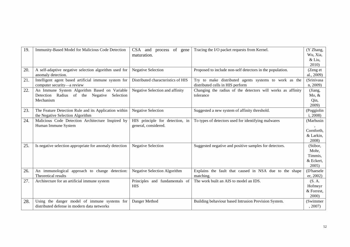
52

19. Immunity-Based Model for Malicious Code Detection CSA and process of gene

maturation.

Tracing the I/O packet requests from Kernel. (Y Zhang,

Wu, Xia,

& Liu,

2010)

20. A self-adaptive negative selection algorithm used for

anomaly detection.

Negative Selection Proposed to include non-self detectors in the population. (Zeng et

al., 2009)

21. Intelligent agent based artificial immune system for

computer security—a review

Distributed characteristics of HIS Try to make distributed agents systems to work as the

distributed cells in HIS perform

(Srinivasa

n, 2009)

22. An Immune System Algorithm Based on Variable

Detection Radius of the Negative Selection

Mechanism

Negative Selection and affinity Changing the radius of the detectors will works as affinity

tolerance

(Jiang,

Mo, &

Qin,

2009)

23. The Feature Detection Rule and its Application within

the Negative Selection Algorithm

Negative Selection Suggested a new system of affinity threshold. (Poggiolin

i, 2008)

24. Malicious Code Detection Architecture Inspired by

Human Immune System

HIS principle for detection, in

general, considered.

To types of detectors used for identifying malwares (Marhusin

,

Cornforth,

& Larkin,

2008)

25. Is negative selection appropriate for anomaly detection Negative Selection Suggested negative and positive samples for detectors. (Stibor,

Mohr,

Timmis,

& Eckert,

2005)

26. An immunological approach to change detection:

Theoretical results

Negative Selection Algorithm Explains the fault that caused in NSA due to the shape

matching.

(D'haesele

er, 2002)

27. Architecture for an artificial immune system Principles and fundamentals of

HIS

The work built an AIS to model an IDS. (S. A.

Hofmeyr

& Forrest,

2000)

28. Using the danger model of immune systems for

distributed defense in modern data networks

Danger Method Building behaviour based Intrusion Prevision System. (Swimmer

, 2007)

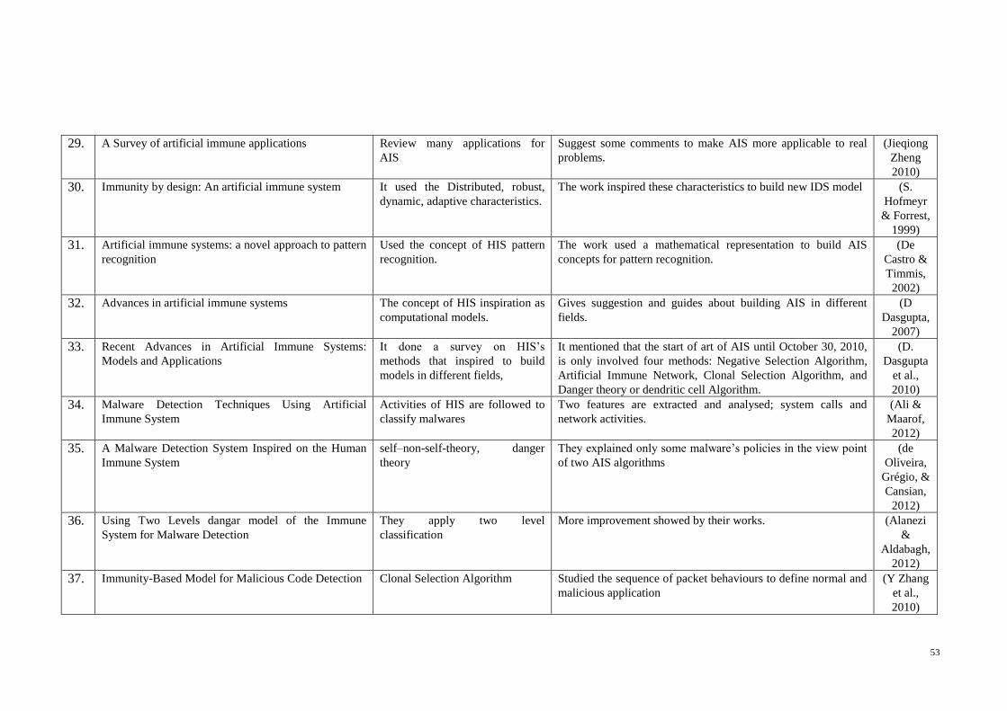
53

29. A Survey of artificial immune applications Review many applications for

AIS

Suggest some comments to make AIS more applicable to real

problems.

(Jieqiong

Zheng

2010)

30. Immunity by design: An artificial immune system It used the Distributed, robust,

dynamic, adaptive characteristics.

The work inspired these characteristics to build new IDS model (S.

Hofmeyr

& Forrest,

1999)

31. Artificial immune systems: a novel approach to pattern

recognition

Used the concept of HIS pattern

recognition.

The work used a mathematical representation to build AIS

concepts for pattern recognition.

(De

Castro &

Timmis,

2002)

32. Advances in artificial immune systems The concept of HIS inspiration as

computational models.

Gives suggestion and guides about building AIS in different

fields.

(D

Dasgupta,

2007)

33. Recent Advances in Artificial Immune Systems:

Models and Applications

It done a survey on HIS’s

methods that inspired to build

models in different fields,

It mentioned that the start of art of AIS until October 30, 2010,

is only involved four methods: Negative Selection Algorithm,

Artificial Immune Network, Clonal Selection Algorithm, and

Danger theory or dendritic cell Algorithm.

(D.

Dasgupta

et al.,

2010)

34. Malware Detection Techniques Using Artificial

Immune System

Activities of HIS are followed to

classify malwares

Two features are extracted and analysed; system calls and

network activities.

(Ali &

Maarof,

2012)

35. A Malware Detection System Inspired on the Human

Immune System

self–non-self-theory, danger

theory

They explained only some malware’s policies in the view point

of two AIS algorithms

(de

Oliveira,

Grégio, &

Cansian,

2012)

36. Using Two Levels dangar model of the Immune

System for Malware Detection

They apply two level

classification

More improvement showed by their works. (Alanezi

&

Aldabagh,

2012)

37. Immunity-Based Model for Malicious Code Detection Clonal Selection Algorithm Studied the sequence of packet behaviours to define normal and

malicious application

(Y Zhang

et al.,

2010)

54

The summary of Table 2-3 could be as follows:

1- The AIS algorithm is used to build many applications in different fields.

2- Many proposed studies in the computer security field employed the AIS. Most

algorithms involved in AIS improve the ability and accuracy of security in

computer systems. The same scenario of HIS has been proposed to integrate

computer immunology or to define defence systems for computers.

3- Regarding malware detection models and approaches, the major AIS

algorithms that are frequently employed include (D. Dasgupta et al., 2010)

a. NSA,

b. AIS network,

c. CSA; and

d. The danger theory and dendritic cell algorithm.

4- Numerous functionalities and phenomena that occur inside HIS are not

included in building malware detection models, including the co-stimulation

phenomenon.

5- The parameters and features that are considered in building bio-oriented

malware detection models differ from case to case.

6- To our knowledge, few studies have employed API calls as features and

parameters to proposed biological detection models.

Biological studies that attempt to classify API call vectors into self- and non-self-groups

have inspired most AIS algorithms, but none of these have involved the co-stimulation

phenomenon to perform such classification despite its importance as a HIS

discrimination method. Response strategies against foreign bodies are adopted based on

the classification achieved by co-stimulation.

55

2.8.3 Why Biological Models?

The main target of any classification model is distinguishing unseen objects to their

correct classes with a high degree of certainty. This target has a direct relation with the

accuracy degree of classifier models. Therefore, the accuracy is the main concern in

classifier models. There are two main features usually related to measure the accuracy

of classifier models, which are FP and FN rates. These two features give indications

about objects that misclassified. Accuracy, as mentioned in Equation 2-1, increases if

FP and FN parameters decrease, and vice versa.

This work focused more on biological models because such models depend on some

processes and strategies of HIS that used to defend body against foreign cells.

Biologically, the strategy that achieved by HIS has no self-cell attacking which means

no FP. Moreover, cases like passing non-self-cell as self-cell, which means FN, is very

rare. Therefore, the accuracy of HIS in classifying self and non-self cells is very high.

The role of having a high accuracy in HIS when classifying foreign cases is going back

to different parts. However for controlling errors, HIS has a phenomenon which

responsible to eliminate errors, and can keep the HIS’s safety with reference to mistakes

made when attacking a self-cell. Although some cells have foreign genes, HIS will not

attack them as non-self-cell as far as they are not harmful cells. It means cells are not

listed as self-cell however have characteristics of self-cells. Distinguishing such

different cells that have similar characteristics by HIS brings attention to this work.

Such type of distinguishing process is very necessary in classify many malicious API

calls that penetrating normal behaviours.

To know more about biological processes inside HIS, and how HIS can keep the

accuracy, latter sections explains the work strategy of HIS and identifies how this

strategy is carried out by HIS.

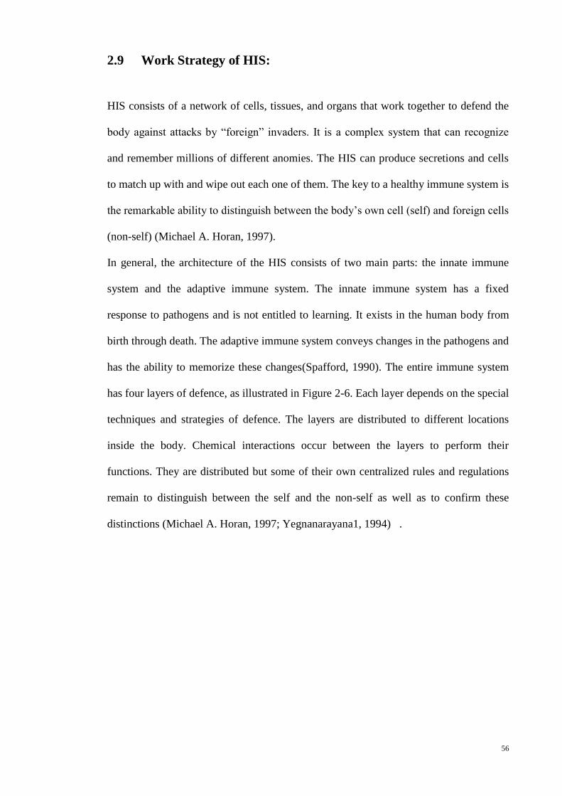
56

2.9 Work Strategy of HIS:

HIS consists of a network of cells, tissues, and organs that work together to defend the

body against attacks by “foreign” invaders. It is a complex system that can recognize

and remember millions of different anomies. The HIS can produce secretions and cells

to match up with and wipe out each one of them. The key to a healthy immune system is

the remarkable ability to distinguish between the body’s own cell (self) and foreign cells

(non-self) (Michael A. Horan, 1997).

In general, the architecture of the HIS consists of two main parts: the innate immune

system and the adaptive immune system. The innate immune system has a fixed

response to pathogens and is not entitled to learning. It exists in the human body from

birth through death. The adaptive immune system conveys changes in the pathogens and

has the ability to memorize these changes(Spafford, 1990). The entire immune system

has four layers of defence, as illustrated in Figure 2-6. Each layer depends on the special

techniques and strategies of defence. The layers are distributed to different locations

inside the body. Chemical interactions occur between the layers to perform their

functions. They are distributed but some of their own centralized rules and regulations

remain to distinguish between the self and the non-self as well as to confirm these

distinctions (Michael A. Horan, 1997; Yegnanarayana1, 1994) .

57

Figure ‎2-6 Layers of the immune system (Michael A. Horan, 1997)

Each layer of the immune system has several functional components known as cells. A

network of interacting cells and molecules, which recognizes foreign substances

(antigens), constitutes the immune system (Michael A. Horan, 1997). The molecules of

the immune system that recognize antigens are called antibodies. An antibody does not

recognize an antigen as an entire object; instead, an antibody recognizes small regions

called epitopes. An antibody recognizes an antigen when it binds to one of its epitopes.

The binding region of an antibody is called the paratope. The strength and specificity of

the interaction between the antibody and the antigen are measured as the affinity of

interaction. The strength of affinity depends on the degree of complementarity in shape

between the interacting regions of the antibody and the antigen. A given antibody can

typically recognize a range of different epitopes, whereas a given epitope can be

recognized by different types of antibodies. An antibody will not only recognize a

specific antigen, but will also recognize other antigens that have the correct epitope. An

epitope characteristic for a given antibody type is called an idiotope (Elgert, 2009).

58

Antibodies produced by cells are called B-lymphocytes. B-lymphocytes differ in terms

of the antibodies they produce. Each type of antibody is produced by a corresponding

lymphocyte, which produces only one type of antibody. When an antibody on the

surface of a lymphocyte binds with another molecule (antigen or other antibody), the

lymphocyte is stimulated to clone and then to secrete free antibodies. In contrast,

lymphocytes that are not stimulated die in a matter of days. Thus, a selection process

occurs whereby antibodies stimulated by antigens increase the antibodies, whereas the

non-stimulated antibodies die (Michael A. Horan, 1997; Spafford, 1990).

Until this stage, the antibodies of the B-cells in the immune system identify non-self-

bodies. However, co-stimulation in the system will confirm whether the decision made

by the B-cell is correct. A positive confirmation will activate B-cells to generate more

of such antibodies and to memorize them; otherwise, a the B-cell decision will be

cancelled and such types of B-cell antibodies will be killed(Yegnanarayana1, 1994).

Such process ensures that no self-cells will be attacked by the immune system, which

results in an autoimmune disease (Michael A. Horan, 1997). To explain more activities

of HIS, next section focused on important functions that occur inside HIS and the task

of each function.

59

2.9.1 Important Activities of HIS

Below are the important activities achieved by the immune cells as well as properties of

the HIS (U Aickelin, Greensmith, & Twycross, 2004):

1- Parallel and Distributed: The structure of the immune system is totally

distributed and has a verity of components. Those components that distributed

throughout the body can communicated through the chemical signals.

2- Multi-layered: No part of the immune system can provide defence

individually. The parts operated independently, yet as a package, to provide

defence to the body.

3- Autonomous: There are many entities at each layer or parts of the immune

system. Each entity has operated independently. This keeps the system

reliability.

4- Imperfect Detection: For detection purposes, not necessary the matching be

exactly, it required exceeding an affinity threshold. It builds detectors so that

they can detect a large subset of non-self-space.

5- Safety: for minimizing the detection errors, there are many checking processes

in the system, such as Co-stimulation (sometimes called second confirmation

signals) and activation thresholds.

6- Diversity: A single pathogen cannot succumb the immune system of entire

population. In addition, a large population of cells with a diverse set of

receptors types enables the body to cover a large portion of the non-self-space.

60

7- Search Space optimizing: The maintenance of the receptors to cover a large

space and changes of search over the time is not an easy job, even though as a

combinatorial. However, the immune system has a great program, through

death and cell division, to maintain a random sampling of the search space.

Therefore, through this program, the immune system always can optimize its

arsenal of receptors.

8- Self / Non-self-Detection: The non-self-receptors death and generation gave the

immune system an ability to detect and respond to pathogens, even those that

have not been countered before.

9- Selective Response: After detection, chemical signals and identification

method effectively classify the antigen. This will determine the exact response

to an infection.

10- Memory: Memory B cells enable the immune system to “remember” past

infections and prime the system for an improve response upon later infection

by the same or similar antigen.

11- Adaptive: The system evolves through clonal selection and hyper-mutation to

improve the antigen recognition capabilities and therefore improve the overall

system performance.

All above functions can be found implicitly in the Figure 2-7 that also shows the

distributed and parallel actions that achieved upon detecting a pathogen (Kim &

Bentley, 2001).

For this work, the safety function that achieved by HIS is more concerned as it controls

FP and FN errors. As mentioned in point number (5), the function that used by HIS to

provide safety and control errors is called co-stimulation. Therefore, the next section

explains in detail how co-stimulation is occurred, biologically, inside HIS.

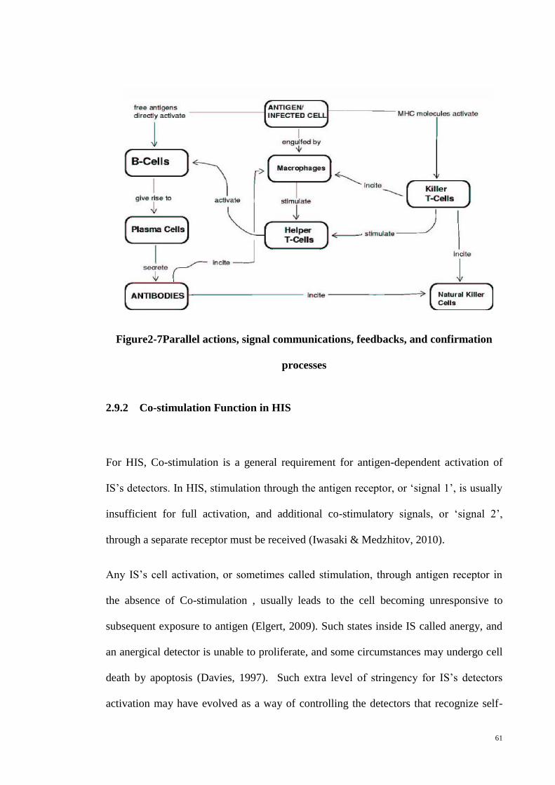
61

Figure‎2-7Parallel actions, signal communications, feedbacks, and confirmation

processes

2.9.2 Co-stimulation Function in HIS

For HIS, Co-stimulation is a general requirement for antigen-dependent activation of

IS’s detectors. In HIS, stimulation through the antigen receptor, or ‘signal 1’, is usually

insufficient for full activation, and additional co-stimulatory signals, or ‘signal 2’,

through a separate receptor must be received (Iwasaki & Medzhitov, 2010).

Any IS’s cell activation, or sometimes called stimulation, through antigen receptor in

the absence of Co-stimulation , usually leads to the cell becoming unresponsive to

subsequent exposure to antigen (Elgert, 2009). Such states inside IS called anergy, and

an anergical detector is unable to proliferate, and some circumstances may undergo cell

death by apoptosis (Davies, 1997). Such extra level of stringency for IS’s detectors

activation may have evolved as a way of controlling the detectors that recognize self-

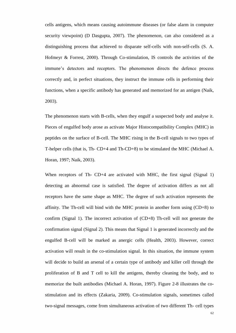
62

cells antigens, which means causing autoimmune diseases (or false alarm in computer

security viewpoint) (D Dasgupta, 2007). The phenomenon, can also considered as a

distinguishing process that achieved to disparate self-cells with non-self-cells (S. A.

Hofmeyr & Forrest, 2000). Through Co-stimulation, IS controls the activities of the

immune’s detectors and receptors. The phenomenon directs the defence process

correctly and, in perfect situations, they instruct the immune cells in performing their

functions, when a specific antibody has generated and memorized for an antigen (Naik,

2003).

The phenomenon starts with B-cells, when they engulf a suspected body and analyse it.

Pieces of engulfed body arose as activate Major Histocompatibility Complex (MHC) in

peptides on the surface of B-cell. The MHC rising in the B-cell signals to two types of

T-helper cells (that is, Th- CD+4 and Th-CD+8) to be stimulated the MHC (Michael A.

Horan, 1997; Naik, 2003).

When receptors of Th- CD+4 are activated with MHC, the first signal (Signal 1)

detecting an abnormal case is satisfied. The degree of activation differs as not all

receptors have the same shape as MHC. The degree of such activation represents the

affinity. The Th-cell will bind with the MHC protein in another form using (CD+8) to

confirm (Signal 1). The incorrect activation of (CD+8) Th-cell will not generate the

confirmation signal (Signal 2). This means that Signal 1 is generated incorrectly and the

engulfed B-cell will be marked as anergic cells (Health, 2003). However, correct

activation will result in the co-stimulation signal. In this situation, the immune system

will decide to build an arsenal of a certain type of antibody and killer cell through the

proliferation of B and T cell to kill the antigens, thereby cleaning the body, and to

memorize the built antibodies (Michael A. Horan, 1997). Figure 2-8 illustrates the co-

stimulation and its effects (Zakaria, 2009). Co-stimulation signals, sometimes called

two-signal messages, come from simultaneous activation of two different Th- cell types

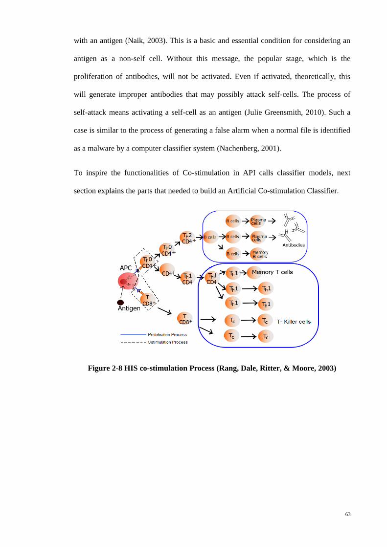
63

with an antigen (Naik, 2003). This is a basic and essential condition for considering an

antigen as a non-self cell. Without this message, the popular stage, which is the

proliferation of antibodies, will not be activated. Even if activated, theoretically, this

will generate improper antibodies that may possibly attack self-cells. The process of

self-attack means activating a self-cell as an antigen (Julie Greensmith, 2010). Such a

case is similar to the process of generating a false alarm when a normal file is identified

as a malware by a computer classifier system (Nachenberg, 2001).

To inspire the functionalities of Co-stimulation in API calls classifier models, next

section explains the parts that needed to build an Artificial Co-stimulation Classifier.

Figure ‎2-8 HIS co-stimulation Process (Rang, Dale, Ritter, & Moore, 2003)

64

2.10 Artificial Co-stimulation Classifier (ACC):

The ACC is a system that depends on the concept of the HIS co-stimulation, structure

and functionalities, to classify malicious API calls in PE malwares. The ACC model

mimics the co-stimulation phenomenon; HIS strongly relies on co-stimulation to

classify self and non-self-cells and to avoid any self-attack (Elgert, 2009). This work

proposes an ACC model to improve the classification of cases that have a strong

similarity index among them, such as the classification of malicious API calls with

normal API calls. Figure 2-9 illustrates the framework of the ACC model that can

distinguish between malicious and normal API calls.

Figure ‎2-9 ACC model to classify malicious API calls

65

As illustrated in Figure 2-9, the ACC model forwards any input case to two different

paths. Through the first path, the model checks the execution sequence of a case,

whereas the second path scans the case to check the availability of four major abnormal

activities done by most malwares. For the first path, the ACC model involves all API

functions that traced and monitored. In the second path, the model narrows down the

monitoring process that divided it into four iterations. For each round, the model checks

the availability of one abnormality behaviour (section 1.7), and it only involves the API

functions mostly used by malwares to achieve an abnormal activity. As explained

below, important issues include the need for both paths and why one path is inadequate

for detecting malicious API calls.

1- First, this work needs narrowing because tracing and monitoring the original

sequences of API calls usually lead to uncertain and misclassified results. In

later chapters, more details on this question are provided.

2- Second, this work needs to keep the results of the first path to identify the certain

and uncertain areas.

3- This work needs narrowing because the API sequence that is applied to the first

path represents the original execution sequence for the suspected application.

The sequence contains a wide range of mixed behaviours, such as junk code

insertion, that usually use jumping among codes. These junk code leads to hide

most malicious behaviours.

4- Narrowing practically means decreasing the number of API functions involved

in an API call monitoring procedure. Most vendors of API call monitoring

software recommend narrowing to obtain results that are more precise. The

reason is that such software might display different results of the sequence of the

API functions called by a suspected application when the number of API

functions involved in monitoring increases or decreases. This problem has been

66

clearly written in the manual of both software used in (APIMonitoring.Com,

2010; HeavenTools, 2010). This present work explains this problem

experimentally in later chapters.

This work depends on artificial neural network (ANN) to construct both checking

blocks (general and narrowing), as illustrated in Figure 2-9. ANN in this work depends

on feed-forward back propagation algorithm during the learning process. The co-

stimulation block uses the Euclidean theory to measure the similarity and the distance

between vectors.

Next two sections explain the theory of tools, ANN and Euclidean methods, that

involved in the process of building the ACC classifier model.

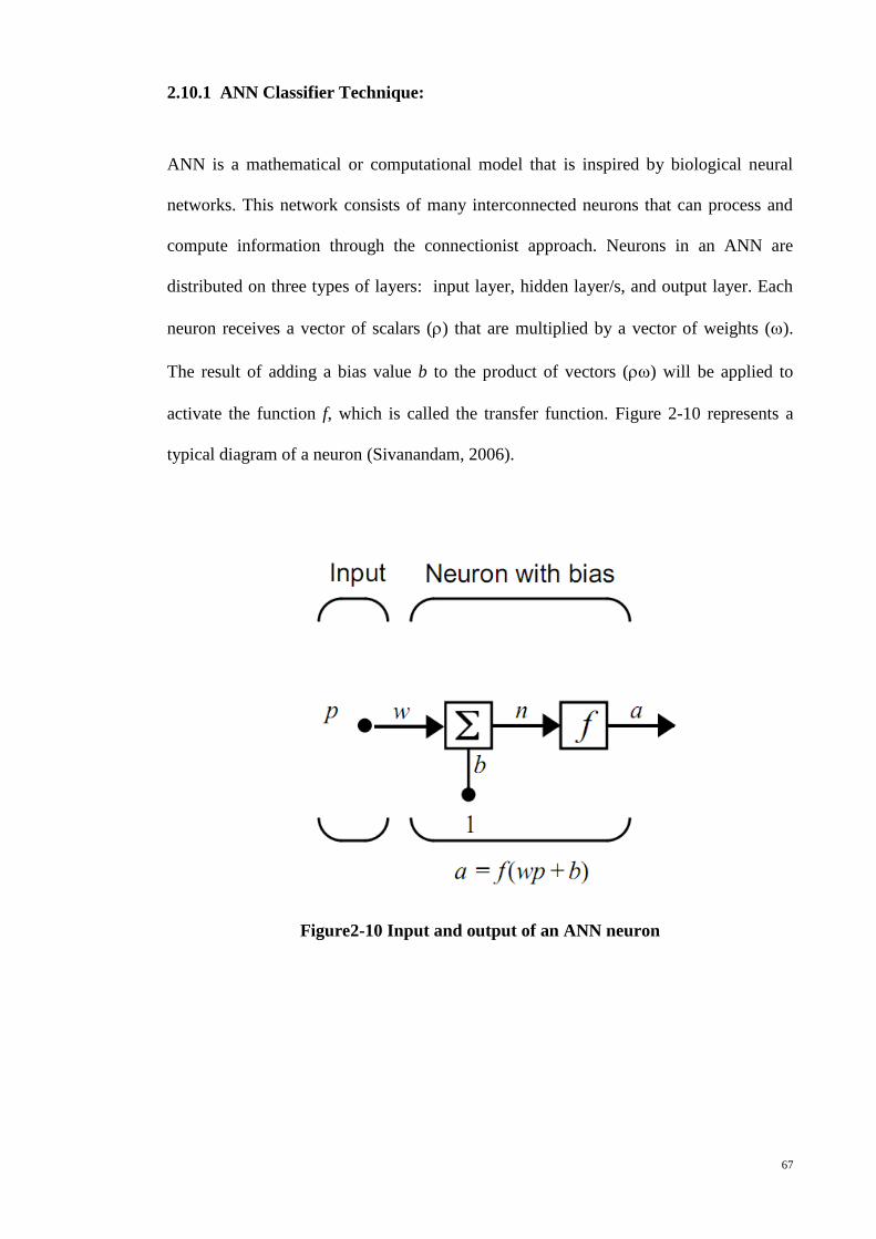
67

2.10.1 ANN Classifier Technique:

ANN is a mathematical or computational model that is inspired by biological neural

networks. This network consists of many interconnected neurons that can process and

compute information through the connectionist approach. Neurons in an ANN are

distributed on three types of layers: input layer, hidden layer/s, and output layer. Each

neuron receives a vector of scalars () that are multiplied by a vector of weights ().

The result of adding a bias value b to the product of vectors () will be applied to

activate the function f, which is called the transfer function. Figure 2-10 represents a

typical diagram of a neuron (Sivanandam, 2006).

Figure‎2-10 Input and output of an ANN neuron

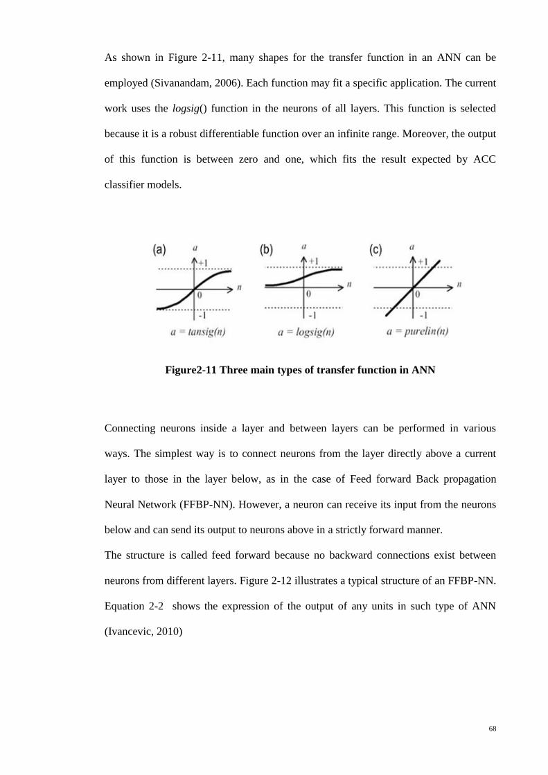
68

As shown in Figure 2-11, many shapes for the transfer function in an ANN can be

employed (Sivanandam, 2006). Each function may fit a specific application. The current

work uses the logsig() function in the neurons of all layers. This function is selected

because it is a robust differentiable function over an infinite range. Moreover, the output

of this function is between zero and one, which fits the result expected by ACC

classifier models.

Figure‎2-11 Three main types of transfer function in ANN

Connecting neurons inside a layer and between layers can be performed in various

ways. The simplest way is to connect neurons from the layer directly above a current

layer to those in the layer below, as in the case of Feed forward Back propagation

Neural Network (FFBP-NN). However, a neuron can receive its input from the neurons

below and can send its output to neurons above in a strictly forward manner.

The structure is called feed forward because no backward connections exist between

neurons from different layers. Figure 2-12 illustrates a typical structure of an FFBP-NN.

Equation 2-2 shows the expression of the output of any units in such type of ANN

(Ivancevic, 2010)

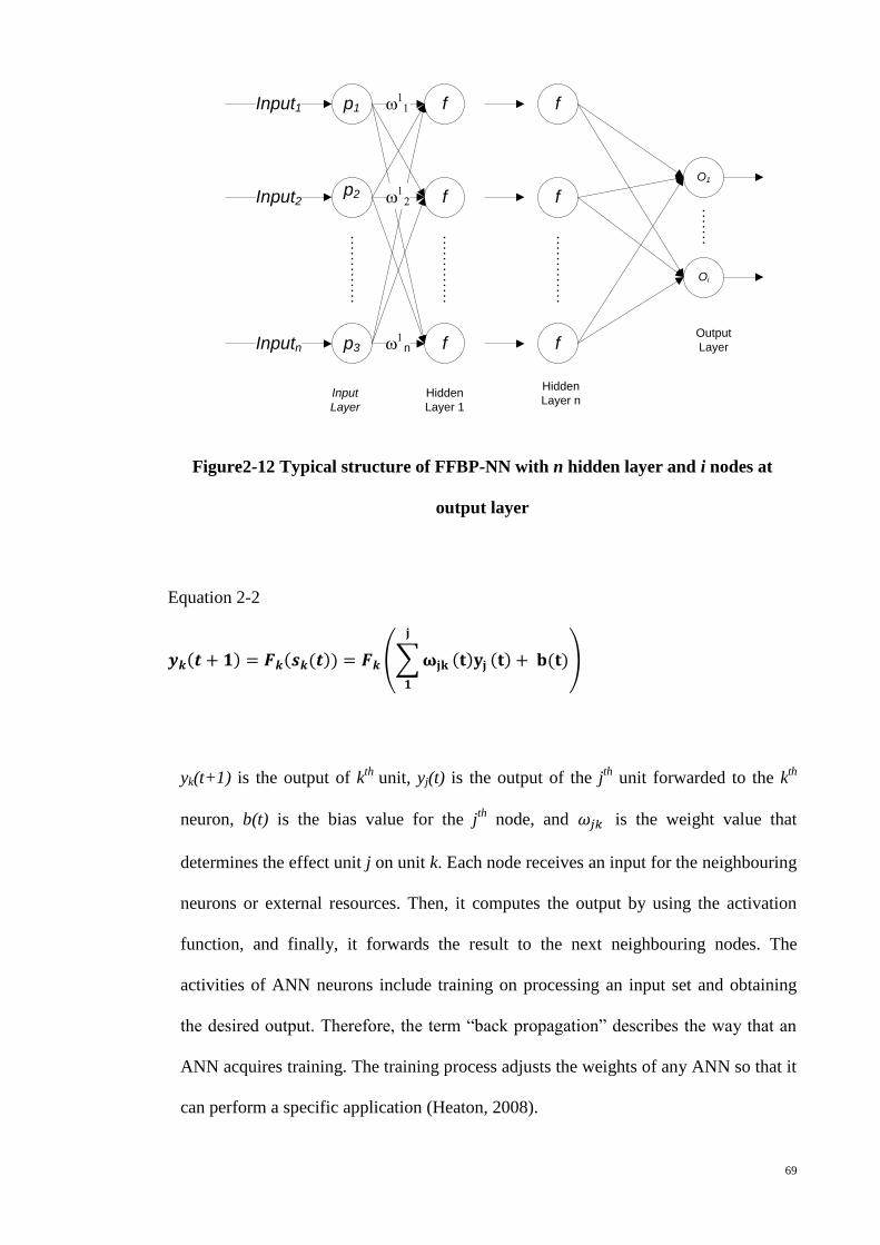
69

p1

p2

p3

f

f

f

f

f

f

O1

Oi

Input1

Input2

Inputn

11

1n

12

Input

Layer

Hidden

Layer 1

Hidden

Layer n

Output

Layer

Figure‎2-12 Typical structure of FFBP-NN with n hidden layer and i nodes at

output layer

Equation 2-2

( ) ( ( )) (∑ ( )

( ) ( ))

yk(t+1) is the output of kth

unit, yj(t) is the output of the jth

unit forwarded to the kth

neuron, b(t) is the bias value for the jth

node, and is the weight value that

determines the effect unit j on unit k. Each node receives an input for the neighbouring

neurons or external resources. Then, it computes the output by using the activation

function, and finally, it forwards the result to the next neighbouring nodes. The

activities of ANN neurons include training on processing an input set and obtaining

the desired output. Therefore, the term “back propagation” describes the way that an

ANN acquires training. The training process adjusts the weights of any ANN so that it

can perform a specific application (Heaton, 2008).

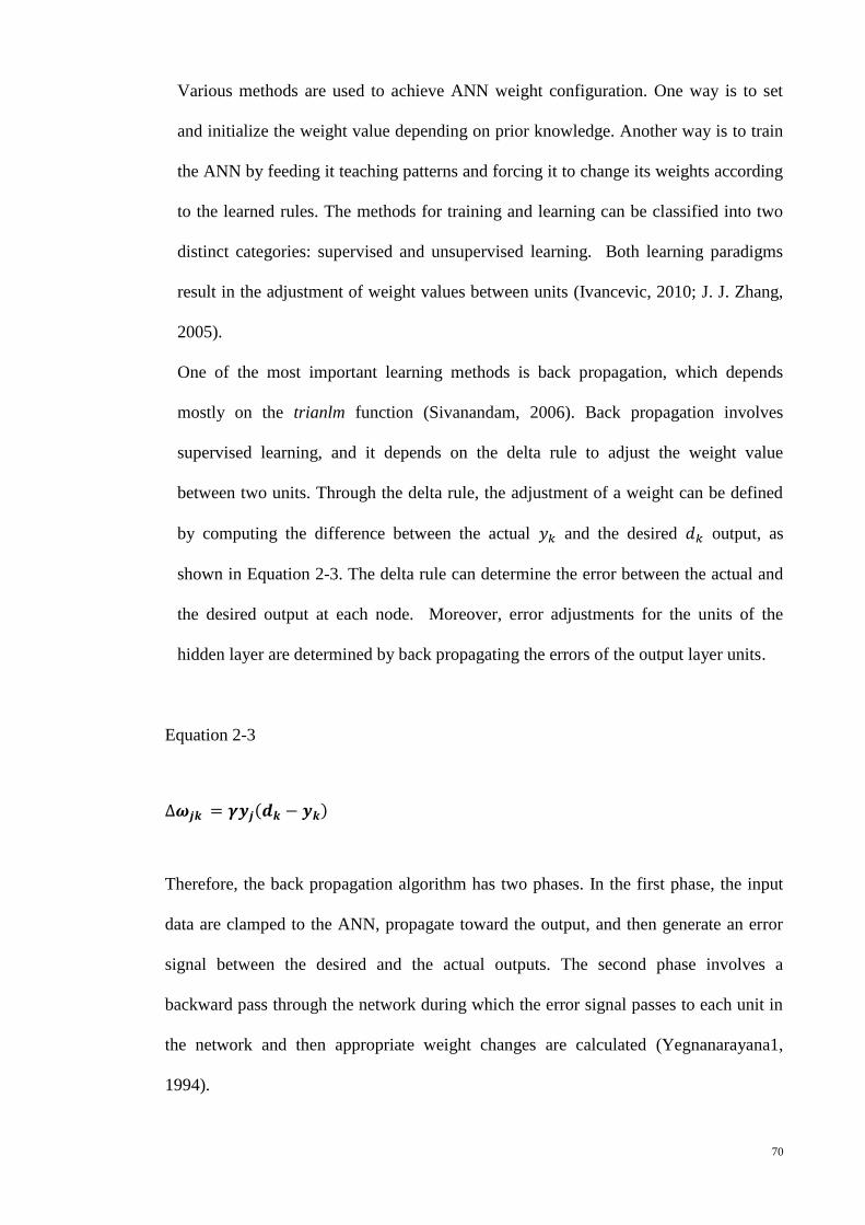
70

Various methods are used to achieve ANN weight configuration. One way is to set

and initialize the weight value depending on prior knowledge. Another way is to train

the ANN by feeding it teaching patterns and forcing it to change its weights according

to the learned rules. The methods for training and learning can be classified into two

distinct categories: supervised and unsupervised learning. Both learning paradigms

result in the adjustment of weight values between units (Ivancevic, 2010; J. J. Zhang,

2005).

One of the most important learning methods is back propagation, which depends

mostly on the trianlm function (Sivanandam, 2006). Back propagation involves

supervised learning, and it depends on the delta rule to adjust the weight value

between two units. Through the delta rule, the adjustment of a weight can be defined

by computing the difference between the actual and the desired output, as

shown in Equation 2-3. The delta rule can determine the error between the actual and

the desired output at each node. Moreover, error adjustments for the units of the

hidden layer are determined by back propagating the errors of the output layer units.

Equation 2-3

( )

Therefore, the back propagation algorithm has two phases. In the first phase, the input

data are clamped to the ANN, propagate toward the output, and then generate an error

signal between the desired and the actual outputs. The second phase involves a

backward pass through the network during which the error signal passes to each unit in

the network and then appropriate weight changes are calculated (Yegnanarayana1,

1994).

71

The rate of error between the actual and the desired outputs will be minimized by

adjusting the value of the neuron’s weight. The overall error that occurred due to

differences between actual and desired for an ANN classifier model is computed

according to the Equation 2-4 (Heaton, 2008).

.

Equation 2-4

√

∑( )

Where:

ti is the desired output and yi is the actual output.

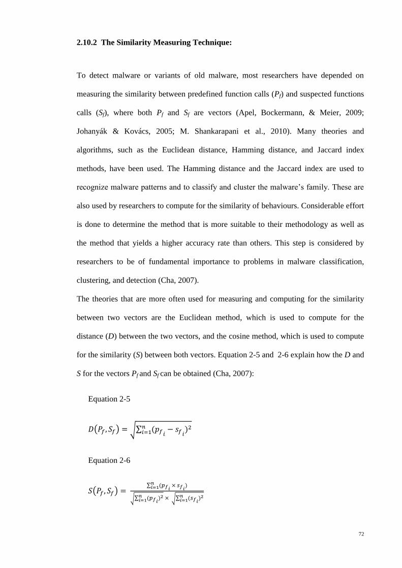
72

2.10.2 The Similarity Measuring Technique:

To detect malware or variants of old malware, most researchers have depended on

measuring the similarity between predefined function calls (Pf) and suspected functions

calls (Sf), where both Pf and Sf are vectors (Apel, Bockermann, & Meier, 2009;

Johanyák & Kovács, 2005; M. Shankarapani et al., 2010). Many theories and

algorithms, such as the Euclidean distance, Hamming distance, and Jaccard index

methods, have been used. The Hamming distance and the Jaccard index are used to

recognize malware patterns and to classify and cluster the malware’s family. These are

also used by researchers to compute for the similarity of behaviours. Considerable effort

is done to determine the method that is more suitable to their methodology as well as

the method that yields a higher accuracy rate than others. This step is considered by

researchers to be of fundamental importance to problems in malware classification,

clustering, and detection (Cha, 2007).

The theories that are more often used for measuring and computing for the similarity

between two vectors are the Euclidean method, which is used to compute for the

distance (D) between the two vectors, and the cosine method, which is used to compute

for the similarity (S) between both vectors. Equation 2-5 and 2-6 explain how the D and

S for the vectors Pf and Sf can be obtained (Cha, 2007):

Equation 2-5

( ) √∑ (

)

Equation 2-6

( ) ∑ (

)

√∑ ( )

√∑ ( )

73

Where n is the number of elements in both vectors, and i is the ith

element within

each vector.

To decide on a similarity status between any two vectors or to obtain the degree of

similarity between them, most studies have considered both values of D and S (Tabish

et al., 2009; S. Yu et al., 2011). However, some studies are satisfied only with one

method to check the affinity status between two compared vectors (Apel et al., 2009; M.

Shankarapani et al., 2010). Although the Euclidean distance method is strongly

recommended by many researchers, the present work states some flaws of this method

(Rozinov, 2005):

1. The Euclidean method depends on the size of the two compared vectors, where

both vectors may be identical, but missing a small part, thereby generating a

high difference in the similarity index.

2. The improper alignment of the two vectors being compared will result in low

Euclidean distance measurement.

However, in our work, the Euclidean method is still applicable given that the size of the

vectors will remain the same. The alignment of vectors is necessary for sequences of

API calls to influence the work.

74

2.11 Chapter Summary

Chapter two could be summarised as below;

1- PE malwares affect the integrity of Windows OS through misusing resources,

such as API call functions.

2- Malware authors can easily find much vulnerability inside PE structure, such as

unused fields and areas that misused by malwares to insert malicious codes.

3- PE malwares can penetrate normal behaviour to avoid classifying their

malicious API call behaviour.

4- Researchers are either depended on biological or non-biological concepts to

devise their malicious API calls classifier models.

5- Penetrating normal calling behaviours by PE malwares brings down the

accuracy of malicious API call classifier models.

6- This work preferred biological concepts of co-stimulation as it can provide

solutions for minimising FP and FN.

7- This work proposed ACC model for classifying malicious API calls in PE

malwares.

8- ACC combines two methods to achieve the concept of co-stimulation; ANN

classifier and Euclidean Similarity theory.

75

Chapter 3

3. Research Methodology

3.1 Introduction

As mentioned in section (2.11), this work proposes ACC model for improving the

accuracy of distinguishing malicious API calls in PE applications. The current chapter

explains the methodology of the ACC model. Throughout this chapter, the main three

parts of the ACC model are explained.

Each parts of the ACC model contains many activities. Although these activities

executed individually and having different aims, they achieved within each part

sequentially. The output of each sub-part is received as an input by subsequent subpart.

Even this sequentially approach is followed between the main parts.

Finally, the input of ACC model is a suspected PE application and the out is its API

calls that classified either normally or maliciously.

Next section starts to explain the works that occurred inside the first part of the ACC

model.

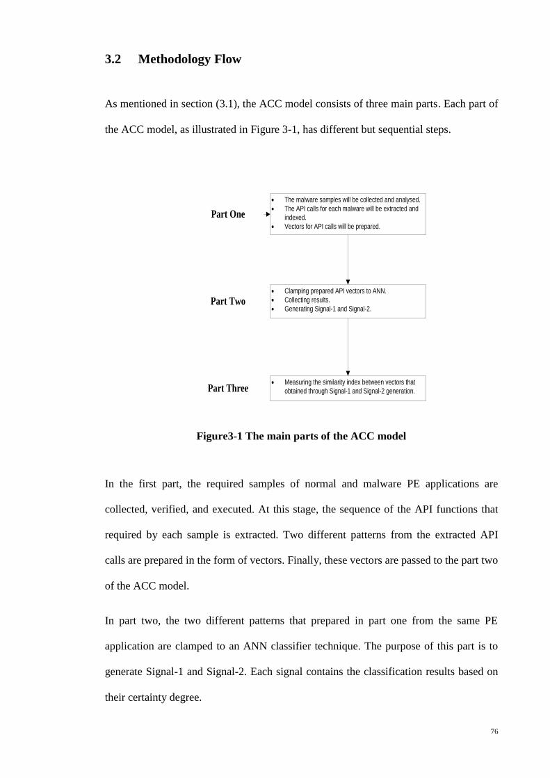
76

3.2 Methodology Flow

As mentioned in section (3.1), the ACC model consists of three main parts. Each part of

the ACC model, as illustrated in Figure 3-1, has different but sequential steps.

Figure‎3-1 The main parts of the ACC model

In the first part, the required samples of normal and malware PE applications are

collected, verified, and executed. At this stage, the sequence of the API functions that

required by each sample is extracted. Two different patterns from the extracted API

calls are prepared in the form of vectors. Finally, these vectors are passed to the part two

of the ACC model.

In part two, the two different patterns that prepared in part one from the same PE

application are clamped to an ANN classifier technique. The purpose of this part is to

generate Signal-1 and Signal-2. Each signal contains the classification results based on

their certainty degree.

· The malware samples will be collected and analysed.

· The API calls for each malware will be extracted and

indexed.

· Vectors for API calls will be prepared.

· Clamping prepared API vectors to ANN.

· Collecting results.

· Generating Signal-1 and Signal-2.

· Measuring the similarity index between vectors that

obtained through Signal-1 and Signal-2 generation.

Part One

Part Two

Part Three

77

Finally, the last part of the ACC model calculates the similarity that may found among

the results that computed in the form of Signal-1 and Signal-2. The purpose of this step

in ACC model is to obtain a new degree of certainty for each misclassified and doubtful

results.

3.3 Part ONE: PE Samples and API Call Vectors

The first part of ACC model, as shown in Figure 3-2, pertains to PE sample collection

and API vectors preparation. This part contains the following steps and activities:

1- For the PE sample collection and preparation, this work achieves that following

steps:

a. Identifying the properties and characteristics of the PE samples that

should be collected as well as the sources where probably could be

found.

b. Verifying all collected PE samples in order to confirm each collected

sample is either malware or normal.

2- For API call vectors preparation, this work achieves the following steps:

a. Extracting the general execution pattern for API calls from the PE

samples that confirmed in the step 1.b.

b. Extracting another four different patterns of API calls from the PE

samples that confirmed in the step 1.b

c. Indexing all API calls that extracted through steps 2.a and 2.b.

d. Preparing API call vectors.

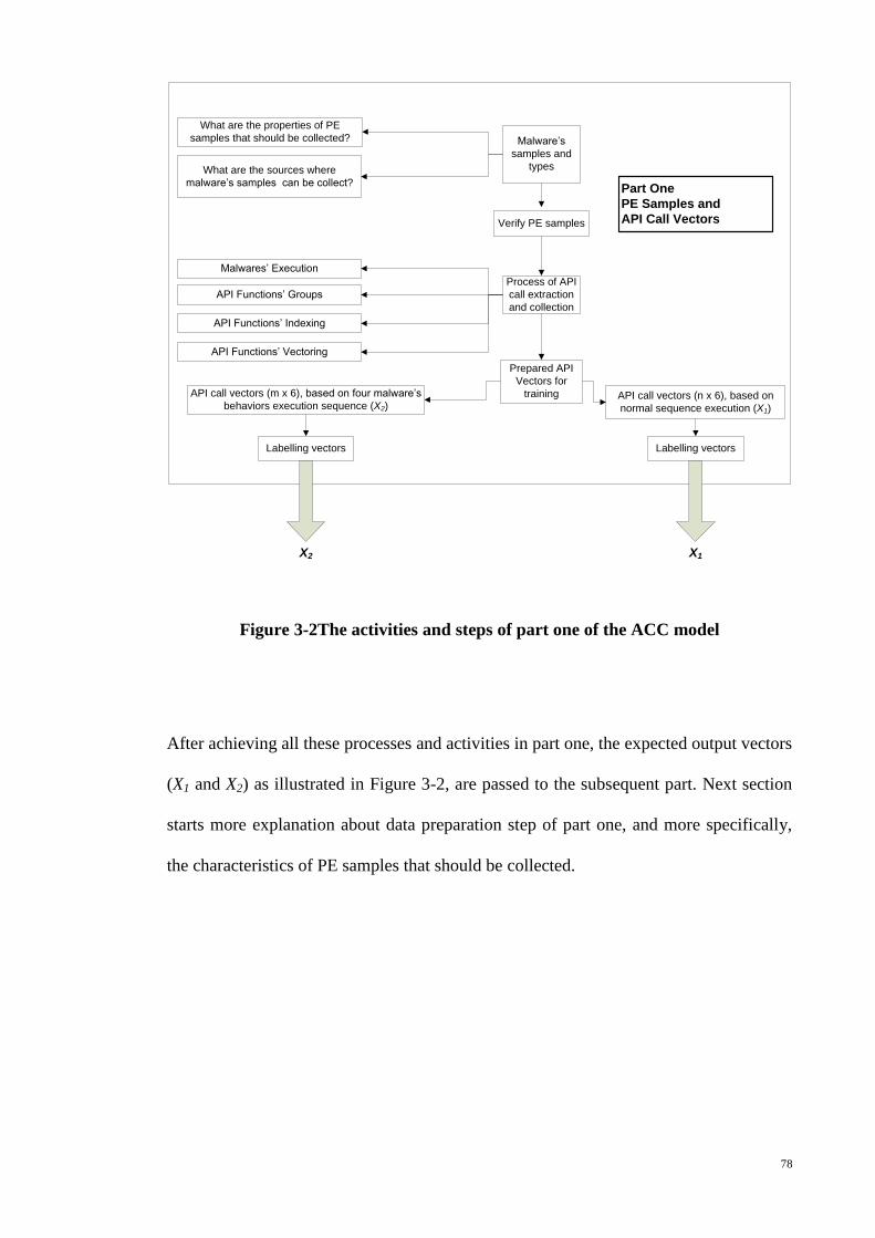
78

Malware’s

samples and

types

What are the properties of PE

samples that should be collected?

What are the sources where

malware’s samples can be collect?

Process of API

call extraction

and collection

Malwares’ Execution

API Functions’ Groups

API Functions’ Indexing

API Functions’ Vectoring

API call vectors (m x 6), based on four malware’s

behaviors execution sequence (X2)

Prepared API

Vectors for

training API call vectors (n x 6), based on

normal sequence execution (X1)

X2 X1

Part One

PE Samples and

API Call VectorsVerify PE samples

Labelling vectors Labelling vectors

Figure ‎3-2The activities and steps of part one of the ACC model

After achieving all these processes and activities in part one, the expected output vectors

(X1 and X2) as illustrated in Figure 3-2, are passed to the subsequent part. Next section

starts more explanation about data preparation step of part one, and more specifically,

the characteristics of PE samples that should be collected.

79

3.3.1 The Properties of PE Malware Samples

This section will focus on three areas as mentioned previously (section 1.7). We have

considered the more frequently infected structure of applications as well as the more

easily penetrated operating systems. Among different types of malware family, this

work covers three families. Therefore, all our samples should share these three

characteristics, as explained and justified below.

1. Regarding the structure and the format of the infected files and application, all

our samples should follow the PE structure because of the following reasons:

a. Many AV vendors reported that 70% to 80% of total malwares are PE

infectors (Ahmadi et al., 2011; Symantec, 2010). Moreover, the

behaviours of one million malwares have been monitored and collected

randomly from networks and the Internet. Research shows that around

80% of malwares have PE infector behaviour (Bayer, Habibi, et al.,

2009).

b. The PE format represents the biggest fraction of today’s malicious

codes. Moreover, a sufficient number of non-malicious samples also

use this format. Therefore, the acquisition of appropriate training and

testing sets is realistic (Merkel et al., 2010).

c. The number of PE infectors throughout past years has been increasing

because the slack and free areas inside these file formats are widely

available, and malware authors can easily misuse them (Essam Al

Daoud, 2008; Schreiber, 2001).

d. It is the valid format that supported by all Windows OS versions

(Microsoft, 2008, 2011).

80

2. All our PE samples are either normal or malware. If the samples are malware,

they should be classified under one of the malware families mentioned in

section 1.7, which includes PE virus, PE Trojan horse, and PE worm. Our

samples have narrowed down the families for the following reasons:

a. These three families are considered as the major types of PE malwares

(AV-Comparative, 2010; McAfee, 2010; McGraw & Morrisett, 2002;

Symantec, 2010; Xu, Sung, Mukkamala, & Liu, 2007).

b. AV vendors have reported that these three groups represent 75% to

85% of the entire population of PE malwares (AV-Comparative, 2010;

Coorp, 2008; McAfee, 2010; Symantec, 2010).

c. Another reason for selecting these categories of malware is because of

the behaviours and activities that could be found in these three types.

Most researchers believe that by evaluating the three behaviours, such

as self or non-self-propagation, dependent or independent execution,

and host or network propagation, the models can reveal most malwares

(K.-S. Han et al., 2011; Niemela & Palomaki, 2011; Trinius et al.,

2011).

d. These three families are the mean families of malwares, and the other

families of malwares could be considered as their sub-families

(Wagener et al., 2008).

3. Our work focuses on Windows OS. Therefore, all our samples should be

Windows-based applications. The reasons for choosing this platform are

explained below:

a. Since the development of the Windows NT version, the PE structure

has become a standardized format for all later versions (Dabak et al.,

1999; Oney, 2002; Schreiber, 2001). Therefore, PE malwares can

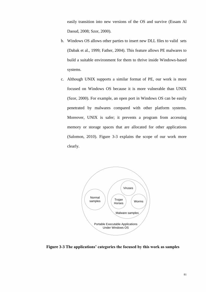
81

easily transition into new versions of the OS and survive (Essam Al

Daoud, 2008; Szor, 2000).

b. Windows OS allows other parties to insert new DLL files to valid sets

(Dabak et al., 1999; Father, 2004). This feature allows PE malwares to

build a suitable environment for them to thrive inside Windows-based

systems.

c. Although UNIX supports a similar format of PE, our work is more

focused on Windows OS because it is more vulnerable than UNIX

(Szor, 2000). For example, an open port in Windows OS can be easily

penetrated by malwares compared with other platform systems.

Moreover, UNIX is safer; it prevents a program from accessing

memory or storage spaces that are allocated for other applications

(Salomon, 2010). Figure 3-3 explains the scope of our work more

clearly.

Portable Executable Applications

Under Windows OS

Normal

samples

Malware samples

Viruses

Trojan

HorsesWorms

Figure ‎3-3 The‎applications’‎categories‎the‎focused‎by‎this‎work‎as‎samples

82

3.3.2 The Sources of PE Samples

In any study, searching for the samples is an important step. However, the type of the

sources where samples could be collected is more important. Researchers have used

different methods to collect normal and malware applications. However, for both types

of application, verification is also an important process.

In collecting PE malwares, one of the resources most researchers use is downloading

the samples from websites. Many online resources provide a substantial number of

normal and malware PE application samples (OffensiveComputing, 2010; VirusSign,

2010; VXHeavens, 2010). However, such samples should be verified. Verification may

be performed by scanning the samples through valid AV software (K.-S. Han et al.,

2011).

This work collected 10,000 samples of PE malware applications from the following

online sources after consulting with the University of Malaya Information Technology

Centre (UMITC).

1- http://vx.netlux.org/vl.php.

2- http://www.offensivecomputing.net/

3- http://www.virussign.com/?gclid=CPv2__m5la0CFUoa6wodWxU0mg

We also collected 2,000 normal PE samples from fresh Windows 7 operating systems.

All samples, comprising normal and malware applications, were collected between May

2010 and September 2010.

Next step of this work shows how and why the collected samples are verified.

http://vx.netlux.org/vl.php

http://www.offensivecomputing.net/

http://www.virussign.com/?gclid=CPv2__m5la0CFUoa6wodWxU0mg

83

3.3.3 PE Samples Verification Process

Most researchers need to verify their malware samples, especially if the malwares were

collected from websites. The research needs verification to determine if the samples are

malwares or not (Szor, 2006). Researchers usually depend on valid AV software to

check the normality or abnormality of suspected samples. To obtain accurate

verification, researchers depend on decisions made by a collection of AV software (H.

Zhao et al., 2010).

To verify our samples, we used five AV software applications, namely, Norton,

KasperSky, McAfee, Avira, and PC-Cillen Internet Security. The first verification

process was implemented using the 2010 version of all AV software. A year later, the

same samples were verified again using the 2011 version of all AV software. The

process of verifying the collected PE samples are clearly illustrated in the Figure3-4.

Table 3-1 provides more details about the number of samples that underwent the

verification process, and the number of malwares that were verified using the five kinds

of AV software. Based on the information listed in the table, some malwares could not

be marked positively by all AV software. The undetected samples are either not

malware or unknown malwares. Therefore, this work only considered those samples

that have been verified as malware by all five AV software to avoid doubts and

uncertainties about the samples.

Hereafter, only 2,000 PE samples; 1,500 PE malwares and 500 normal applications

were considered for further works in this study. Verified samples of PE malwares are

divided into 500 PE viruses, 500 PE Trojan horses, and 500 PE worms. The numbers of

collected samples, which are 2,000, are confirmed by(Parmjit Singh, Chan Yuen Fook,

& Sidhu, 2009)as a sufficient number for building ACC model. Only samples that

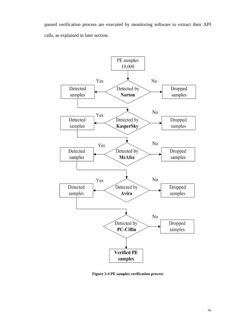
84

passed verification process are executed by monitoring software to extract their API

calls, as explained in later section.

Figure ‎3-4 PE samples verification process

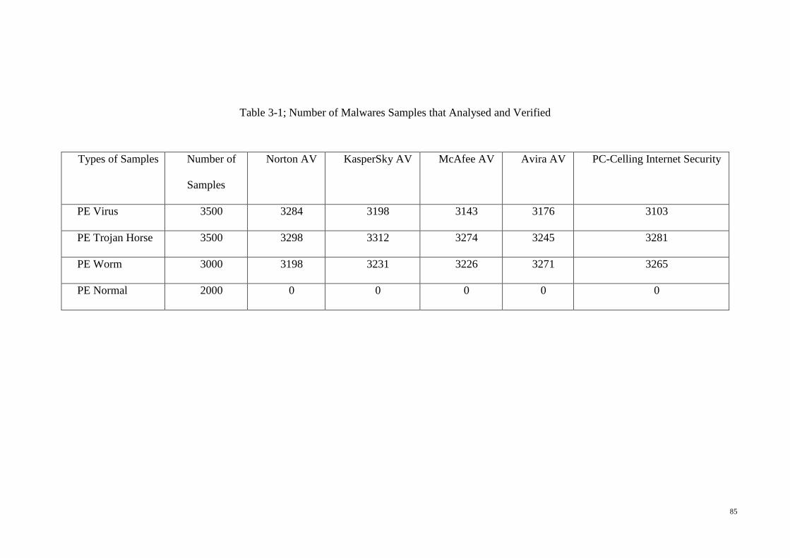
85

Table 3-1; Number of Malwares Samples that Analysed and Verified

Types of Samples Number of

Samples

Norton AV KasperSky AV McAfee AV Avira AV PC-Celling Internet Security

PE Virus 3500 3284 3198 3143 3176 3103

PE Trojan Horse 3500 3298 3312 3274 3245 3281

PE Worm 3000 3198 3231 3226 3271 3265

PE Normal 2000 0 0 0 0 0

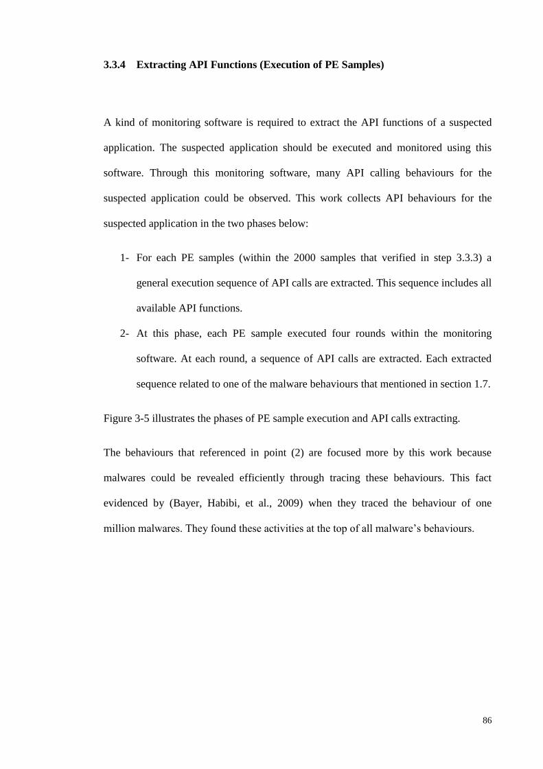
86

3.3.4 Extracting API Functions (Execution of PE Samples)

A kind of monitoring software is required to extract the API functions of a suspected

application. The suspected application should be executed and monitored using this

software. Through this monitoring software, many API calling behaviours for the

suspected application could be observed. This work collects API behaviours for the

suspected application in the two phases below:

1- For each PE samples (within the 2000 samples that verified in step 3.3.3) a

general execution sequence of API calls are extracted. This sequence includes all

available API functions.

2- At this phase, each PE sample executed four rounds within the monitoring

software. At each round, a sequence of API calls are extracted. Each extracted

sequence related to one of the malware behaviours that mentioned in section 1.7.

Figure 3-5 illustrates the phases of PE sample execution and API calls extracting.

The behaviours that referenced in point (2) are focused more by this work because

malwares could be revealed efficiently through tracing these behaviours. This fact

evidenced by (Bayer, Habibi, et al., 2009) when they traced the behaviour of one

million malwares. They found these activities at the top of all malware’s behaviours.

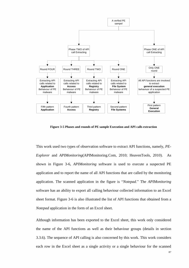
87

A verfied PE

sampel

Phase ONE of API

call Extracting

All API functions are involved

to extract

general execution

behaviuor of a suspected PE

application

Phase TWO of API

call Extracting

Round ONERound TWORound THREERound FOUR

Extracting API

calls related to

Application

Behaivour of PE

malware

Extracting API

calls related to

Access

Behaivour of PE

malware

Extracting API

calls related to

Registry

Behaivour of PE

malware

Extracting API

calls related to

File System

Behaivour of PE

malware

First pattern

General

Execution

Second pattern

File Systems

Third pattern

Registry

Fourth pattern

Access

Fifth pattern

Application

Only ONE

round

Figure ‎3-5 Phases and rounds of PE sample Execution and API calls extraction

This work used two types of observation software to extract API functions, namely, PE-

Explorer and APIMonitoring(APIMonitoring.Com, 2010; HeavenTools, 2010). As

shown in Figure 3-6, APIMonitoring software is used to execute a suspected PE

application and to report the name of all API functions that are called by the monitoring

application. The scanned application in the figure is “Notepad.” The APIMonitoring

software has an ability to export all calling behaviour collected information to an Excel

sheet format. Figure 3-6 is also illustrated the list of API functions that obtained from a

Notepad application in the form of an Excel sheet.

Although information has been exported to the Excel sheet, this work only considered

the name of the API functions as well as their behaviour groups (details in section

3.3.6). The sequence of API calling is also concerned by this work. This work considers

each row in the Excel sheet as a single activity or a single behaviour for the scanned

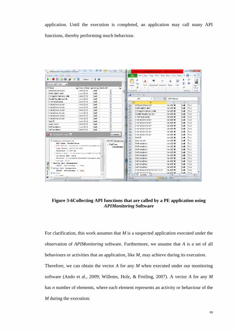
88

application. Until the execution is completed, an application may call many API

functions, thereby performing much behaviour.

Figure ‎3-6Collecting API functions that are called by a PE application using

APIMonitoring Software

For clarification, this work assumes that M is a suspected application executed under the

observation of APIMonitoring software. Furthermore, we assume that A is a set of all

behaviours or activities that an application, like M, may achieve during its execution.

Therefore, we can obtain the vector A for any M when executed under our monitoring

software (Ando et al., 2009; Willems, Holz, & Freiling, 2007). A vector A for any M

has n number of elements, where each element represents an activity or behaviour of the

M during the execution:

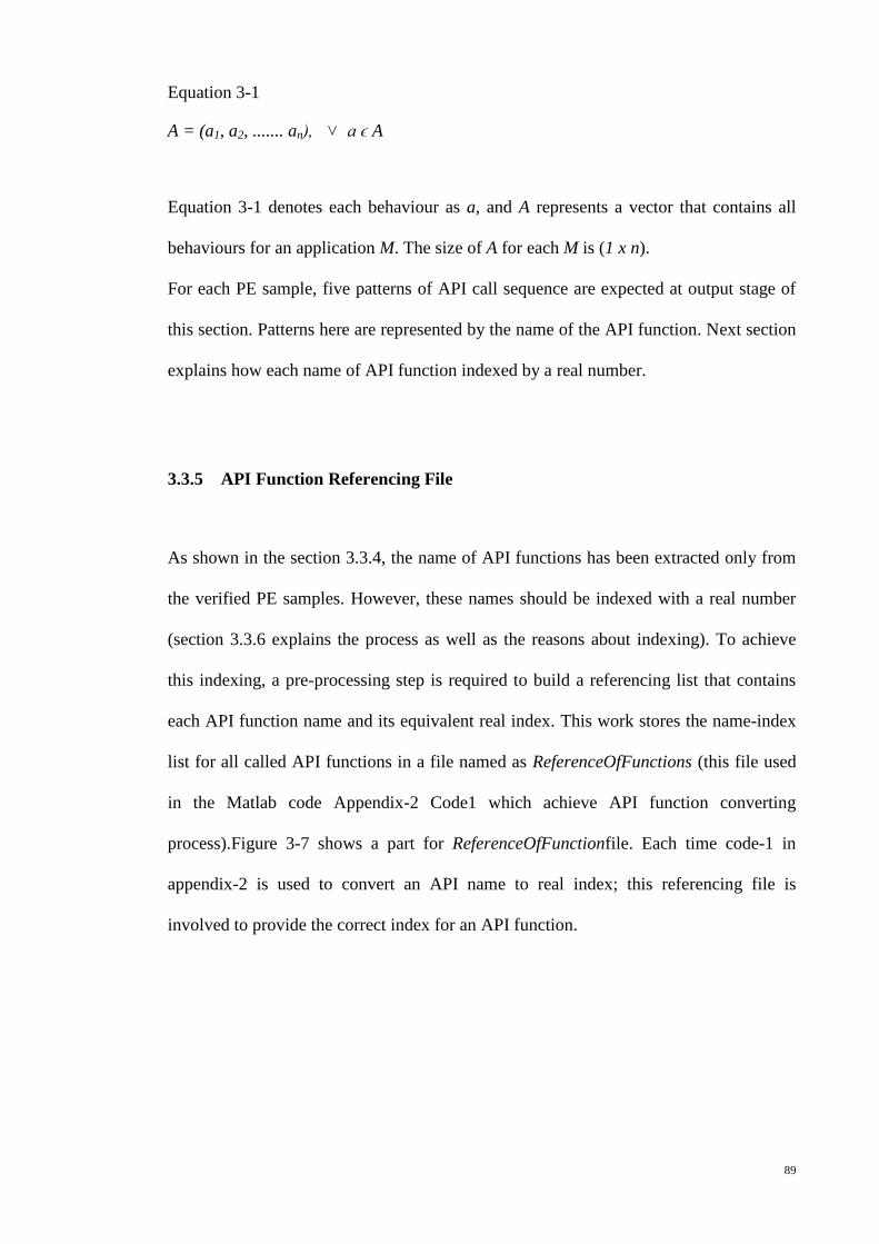
89

Equation 3-1

A = (a1, a2, ....... an), ˅ a ϵ A

Equation 3-1 denotes each behaviour as a, and A represents a vector that contains all

behaviours for an application M. The size of A for each M is (1 x n).

For each PE sample, five patterns of API call sequence are expected at output stage of

this section. Patterns here are represented by the name of the API function. Next section

explains how each name of API function indexed by a real number.

3.3.5 API Function Referencing File

As shown in the section 3.3.4, the name of API functions has been extracted only from

the verified PE samples. However, these names should be indexed with a real number

(section 3.3.6 explains the process as well as the reasons about indexing). To achieve

this indexing, a pre-processing step is required to build a referencing list that contains

each API function name and its equivalent real index. This work stores the name-index

list for all called API functions in a file named as ReferenceOfFunctions (this file used

in the Matlab code Appendix-2 Code1 which achieve API function converting

process).Figure 3-7 shows a part for ReferenceOfFunctionfile. Each time code-1 in

appendix-2 is used to convert an API name to real index; this referencing file is

involved to provide the correct index for an API function.

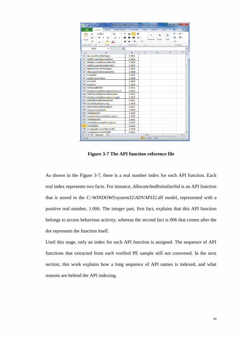
90

.

Figure ‎3-7 The API function reference file

As shown in the Figure 3-7, there is a real number index for each API function. Each

real index represents two facts. For instance, AllocateAndInitializeSid is an API function

that is stored in the C:\WINDOWS\system32\ADVAPI32.dll model, represented with a

positive real number, 1.006. The integer part, first fact, explains that this API function

belongs to access behaviour activity, whereas the second fact is 006 that comes after the

dot represents the function itself.

Until this stage, only an index for each API function is assigned. The sequence of API

functions that extracted from each verified PE sample still not converted. In the next

section, this work explains how a long sequence of API names is indexed, and what

reasons are behind the API indexing.

91

3.3.6 Indexing the observed API Functions

As mentioned in section 3.3.5, this work needs to convert each element in A (section

3.3.4) that represents the name of an API function to a real number index. The reason

that behind indexing the name of API function calls is because dealing with a real

number is easier than dealing with strings, especially, if such information clamps any

artificial intelligent (AI) technique. Most researchers that employed an AI technique as

a classifier model have converted the name of all API functions from strings to integers

or any real number (Zolkipli & Jantan, 2011).

When a Matlab code, such as mentioned in Appendix-2 / code1, is used to convert the

name of an API function, it reads first the name of the API function that needs to be

converted. Then, the code makes a search inside the ReferenceOfFunction to find out its

equivalent index value. Finally, the code sends out the correct index.

To explain indexing API functions mathematically, suppose I(x) denotes the indexing

function that converts strings (API function) to their equivalent indices, which are real

numbers, then,

Equation 3-2

I (A) = ( I(a1), I(a2)…I(an) )

and each string a is converted to r real number,

I(ai) ri ˅ r ϵ R Or I(A)

where ri is the equivalent index of the ai API function and it is the ith

element in the

vector. The output of the indexing process is a vector that has the same (1 x n)

dimensions. This result indicates that vectors A and have the same dimensions.

However, for each pattern that obtained in section 3.3.4, the value of n is difference.

92

Next stage shows converting the long sequence of API indexes to matrixes through

scanning-sliding process.

3.3.7 Scanning –Sliding the Indexing API calls

At this stage, we need to convert the vector , which has (1x n) dimension to a matrix

with dimension of (m x 6) because we need to build two data sets in the form of

matrices, X1, to generate Signal-1, and X2, to generate Signal-2 (Figure 3-2). Both input

sets are derived from vector .

The size of vectors in the new matrix should be established to convert a long sequence

of indexed API functions into a matrix. The size of the vector denotes the number of

elements inside each vector. The number of elements inside each vector identifies the

adequate number of indexed API calls to reveal malware behaviour. Most researchers

set this number to six elements (Alanezi & Aldabagh, 2012). Six elements from the long

sequence of an indexed API calls vector are scanned each time. After scanning, the

scanning window slides by one unit. This process will continue until scanning of the last

six elements of a long indexed API call is completed.

The scanning–sliding process described above is followed to form both X1 and X2

datasets, however, with a little difference. In forming X1, Figure3-8 illustrates the

process of scanning–sliding on the indexed API calls of an application. The scanning

window is shown at three positions. At each position, the process scans only six indexed

API calls. Then, the process copies the content of this window to make a new vector in

input set X1.

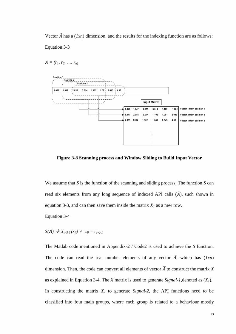
93

Vector has a (1xn) dimension, and the results for the indexing function are as follows:

Equation 3-3

= (r1, r2, …. rn)

Figure ‎3-8 Scanning process and Window Sliding to Build Input Vector

We assume that S is the function of the scanning and sliding process. The function S can

read six elements from any long sequence of indexed API calls ( ), such shown in

equation 3-3, and can then save them inside the matrix X1 as a new row.

Equation 3-4

S( ) Xn-5 6 (xij) ˅ xij = ri+j-1

The Matlab code mentioned in Appendix-2 / Code2 is used to achieve the S function.

The code can read the real number elements of any vector , which has (1xn)

dimension. Then, the code can convert all elements of vector to construct the matrix X

as explained in Equation 3-4. The X matrix is used to generate Signal-1,denoted as (X1).

In constructing the matrix X2 to generate Signal-2, the API functions need to be

classified into four main groups, where each group is related to a behaviour mostly

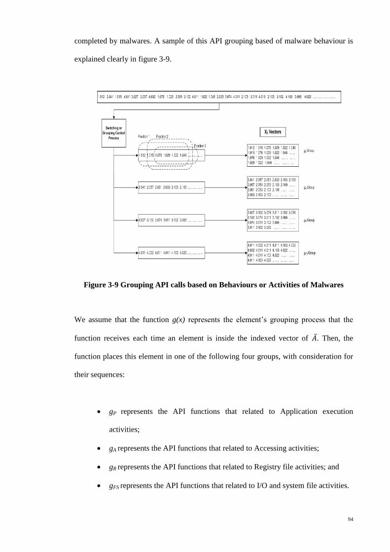
94

completed by malwares. A sample of this API grouping based of malware behaviour is

explained clearly in figure 3-9.

Figure ‎3-9 Grouping API calls based on Behaviours or Activities of Malwares

We assume that the function g(x) represents the element’s grouping process that the

function receives each time an element is inside the indexed vector of . Then, the

function places this element in one of the following four groups, with consideration for

their sequences:

· gP represents the API functions that related to Application execution

activities;

· gA represents the API functions that related to Accessing activities;

· gR represents the API functions that related to Registry file activities; and

· gFS represents the API functions that related to I/O and system file activities.

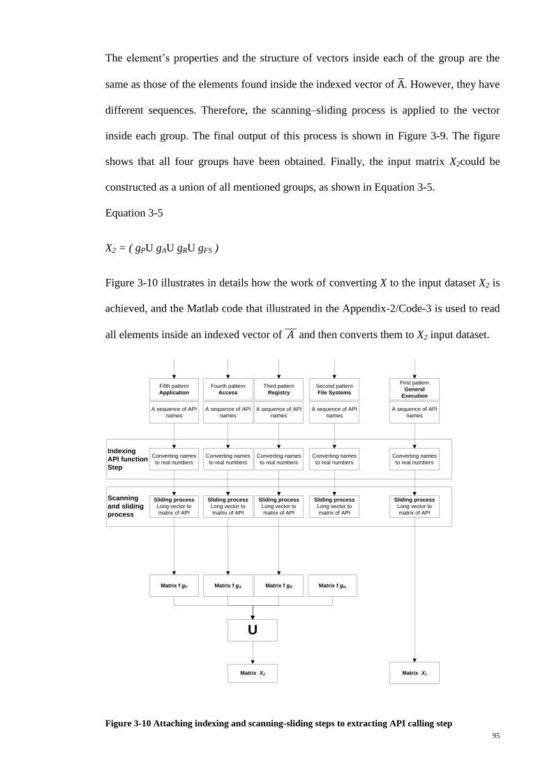
95

The element’s properties and the structure of vectors inside each of the group are the

same as those of the elements found inside the indexed vector of . However, they have

different sequences. Therefore, the scanning–sliding process is applied to the vector

inside each group. The final output of this process is shown in Figure 3-9. The figure

shows that all four groups have been obtained. Finally, the input matrix X2could be

constructed as a union of all mentioned groups, as shown in Equation 3-5.

Equation 3-5

X2 = ( gPU gAU gRU gFS )

Figure 3-10 illustrates in details how the work of converting X to the input dataset X2 is

achieved, and the Matlab code that illustrated in the Appendix-2/Code-3 is used to read

all elements inside an indexed vector of and then converts them to X2 input dataset.

First pattern

General

Execution

Second pattern

File Systems

Third pattern

Registry

Fourth pattern

Access

Fifth pattern

Application

A sequence of API

names

A sequence of API

names

A sequence of API

names

A sequence of API

names

A sequence of API

names

Converting names

to real numbers

Converting names

to real numbers

Converting names

to real numbers

Converting names

to real numbers

Converting names

to real numbers

Indexing

API function

Step

Sliding process

Long vector to

matrix of API

Scanning

and sliding

process

Sliding process

Long vector to

matrix of API

Sliding process

Long vector to

matrix of API

Sliding process

Long vector to

matrix of API

Sliding process

Long vector to

matrix of API

Matrix X1

Matrix f gRMatrix f gAMatrix f gP

U

Matrix X2

Matrix f gfs

Figure ‎3-10 Attaching indexing and scanning-sliding steps to extracting API calling step

96

The output of this part is generating both X1 and X2 data sets. Next section is about the

methodology of the part two that used both prepared data sets to generate Signal-1 and

Signal-2.

3.3.8 Labelling vectors in X1 and X2:

Each vector in X1 and X2 represented the behaviour of the six calls made by a PE

application. Therefore, the class to which a vector belonged, namely, normal or

malware, must be identified. Each vector needed to be labelled by identifying their

classes. Each vector class is labelled either as (0) or as (1). The label (0) is considered

for normal calls, whereas label (1) is considered for malicious calls.

Different levels of binary for labelling were used to identify the family of each malware

vector. However, the family identification of malware applications was beyond the

scope of this research. This labelling process helped our model during the training and

testing phases. The model used these labelling processes as a target for each vector,

which is usually what a supervised ANN needs during implementation (Sivanandam,

2006).

The implementation of Part One of the ACC model is thus completed. Prepared

matrixes of X1 and X2 will be forwarded to the next part. At later parts, the list of below

will be expected:

1- The ACC model uses both datasets in the processes of training or test-setting

phases;

2- A part of a prepared dataset will be used to test the accuracy and error problems

of some classifier models;

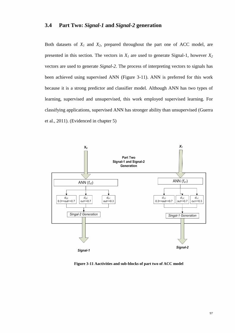
97

3.4 Part Two: Signal-1 and Signal-2 generation

Both datasets of X1 and X2, prepared throughout the part one of ACC model, are

presented in this section. The vectors in X1 are used to generate Signal-1, however X2

vectors are used to generate Signal-2. The process of interpreting vectors to signals has

been achieved using supervised ANN (Figure 3-11). ANN is preferred for this work

because it is a strong predictor and classifier model. Although ANN has two types of

learning, supervised and unsupervised, this work employed supervised learning. For

classifying applications, supervised ANN has stronger ability than unsupervised (Guerra

et al., 2011). (Evidenced in chapter 5)

Figure ‎3-11 Aactivities and sub-blocks of part two of ACC model

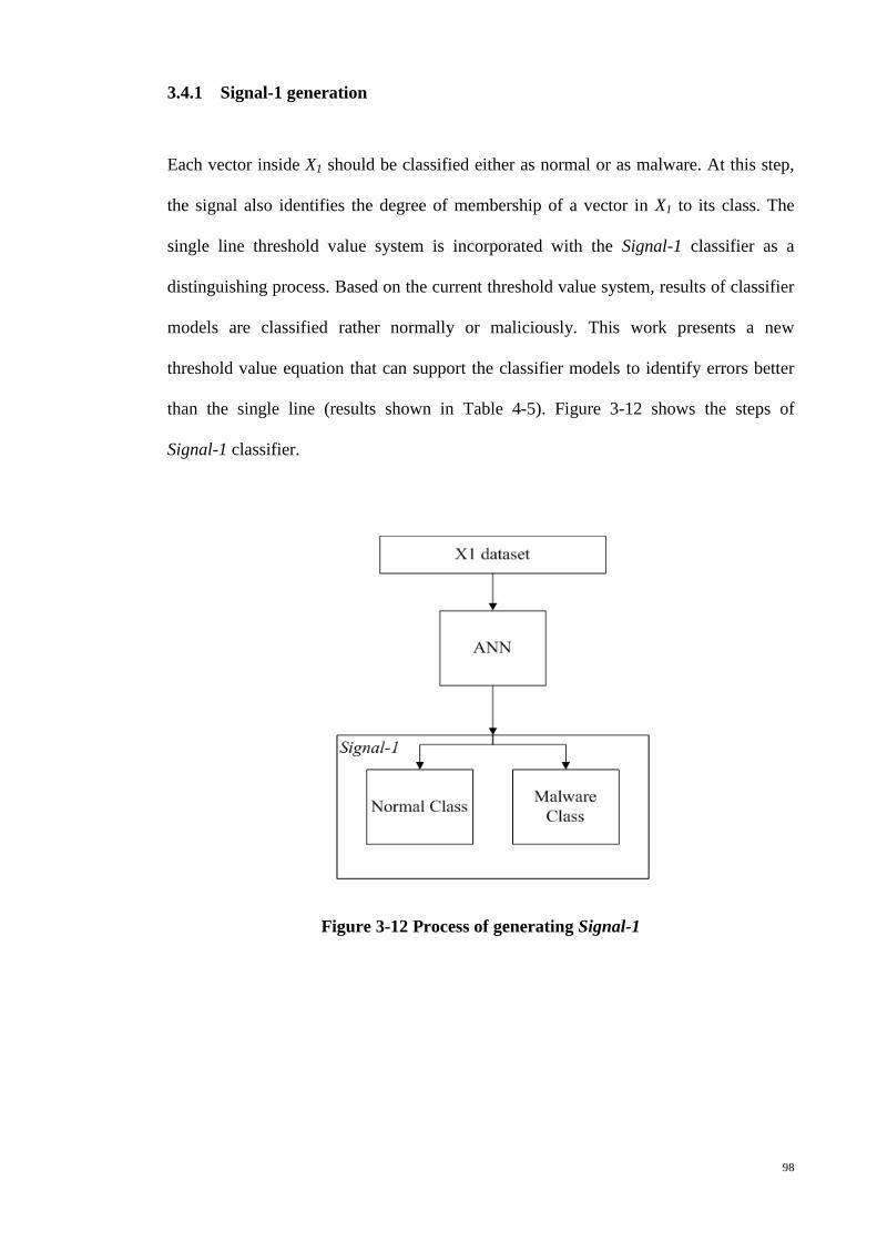
98

3.4.1 Signal-1 generation

Each vector inside X1 should be classified either as normal or as malware. At this step,

the signal also identifies the degree of membership of a vector in X1 to its class. The

single line threshold value system is incorporated with the Signal-1 classifier as a

distinguishing process. Based on the current threshold value system, results of classifier

models are classified rather normally or maliciously. This work presents a new

threshold value equation that can support the classifier models to identify errors better

than the single line (results shown in Table 4-5). Figure 3-12 shows the steps of

Signal-1 classifier.

Figure ‎3-12 Process of generating Signal-1

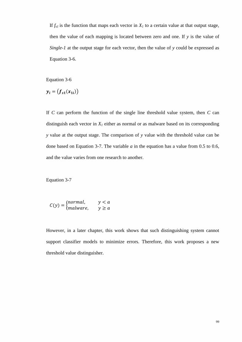
99

If fs1 is the function that maps each vector in X1 to a certain value at that output stage,

then the value of each mapping is located between zero and one. If y is the value of

Single-1 at the output stage for each vector, then the value of y could be expressed as

Equation 3-6.

Equation 3-6

( ( ))

If C can perform the function of the single line threshold value system, then C can

distinguish each vector in X1 either as normal or as malware based on its corresponding

y value at the output stage. The comparison of y value with the threshold value can be

done based on Equation 3-7. The variable a in the equation has a value from 0.5 to 0.6,

and the value varies from one research to another.

Equation 3-7

( ) {

However, in a later chapter, this work shows that such distinguishing system cannot

support classifier models to minimize errors. Therefore, this work proposes a new

threshold value distinguisher.

100

Based on the new threshold system that shown in Equation 3-8, outputs of Signal-1 can

be divided into three area, namely, d11, d12, and d13:

Equation 3-8

( ) {

Signal-1 carries three different classes (d11, d12, and d13) as outputs. This work focuses

more on the elements that lay in d13 area because all elements of this group are

considered either as doubtful or as misclassified objects.

Finally, the input vectors of X1 are classified into three groups of (G1), namely, normal

vectors (G1n), malware vectors (G1m), and suspected vectors (G1s). The work groups of

each input vector based on their corresponding output ( ).

If G is the function of the groups in the input vectors, as in equation 3-9, then the final

stage Signal-1 maintains for any vector in X1 includes the input vector itself X1i, the

actual output y1i, and the group of the input vector G1i, Equation 3-10.

Equation 3-9

( ) {

Equation 3-10

( ) (

)

More details on the execution of Signal-1 will be discussed in chapter four. Next section

explains the process of preparing Signla-2 results.

101

3.4.2 Signal-2 generation

The same ANN used to generate Signal-1 is also employed to generate Signal-2 because

the structure of the input dataset X2 is exactly similar to that of X1. Each vector in X2 has

six real value elements, as in X1. The process of training and testing the ANN is also the

same. However, each vector in X2 represents a different aspect from the vectors of X1.

Although the meaning of vectors is not the same, the target of each vector in X2 is

represented by 0 or 1, implying the same range of output. Therefore, the activation

function used by each node for training X1 has not changed during the training of X2.

Due to the difference in the meaning of vectors in both datasets, the output of the ANN

gives different explanation. The execution of the ANN with X2 determines the degree of

relationship between each vector with certain malware behaviours. However, the

execution of the same ANN with X1, can only show the degree of normality of a general

execution vector. More importantly, ANN with X2 can classify malwares, implicitly,

based on the four major behaviours of malwares. However, this goal is beyond of our

work. ANN with X2 checks vectors for a specific behaviour; hence, precise results could

be obtained.

The results of Signal-2 are distinguished also based on Equation 3-8. Moreover,

Equation 3-9 is used for grouping the vectors of X2 into three groups in (G2), such as

normal vectors (G2n), malware vectors (G2m), and suspected vectors (G2s).

Equation 3-10 is used to generating Signal-2 for each vector in X2. The format of

Signal-2 can be shown as (X2i, Y2i, G2i). However, sub-classification exists inside each

group. Vectors in each group will belong to one of monitored behaviours of the

malware. Based on the monitored behaviour of an application, we can determine if the

application is a malware or not.

Next section explains how results of Signal-1 and Signal-2 proceeds by the part three of

ACC model.

102

3.5 Part Three: Co-stimulation

In this part, ACC model performs a comparison process between elements of Signal-1

and Signal-2. For Signal-1, only cases in d13 are considered. However, for Signal-2,

cases in both d21 and d22 are considered. The model takes each case in d13 (suppose Ci),

and achieves the following procedures:

1- Compute the similarity index between Ci and each case in d21. Then;

a. Considerer only vectors that their similarity indexes are greater than 0.7.

b. Compute the total number of vectors that obtained in 1.a.

c. Compare the number that obtained in 1.b with the factor K (value of K

explained later page 178, 3).

2- Compute the similarity index between Ci and each element in d22, and then

repeat all steps of 1.a, 1.b, and1.c to obtain 2.a, 2.b, and 2.c.

3- ACC makes decision based on the following rules:

Table ‎3-2 Rules that considered during signals confirmation.

Status of Ci Rules

Ci is Normal

If the value that obtained in 1.b >K (Signal-1 confirmation) and

value that obtained in 2.b <K (Signal-2 confirmation).

Ci is Malware

If the value that obtained in 1.b <K (Signal-1 confirmation) and

value that obtained in 2.b >K (Signal-2 confirmation).

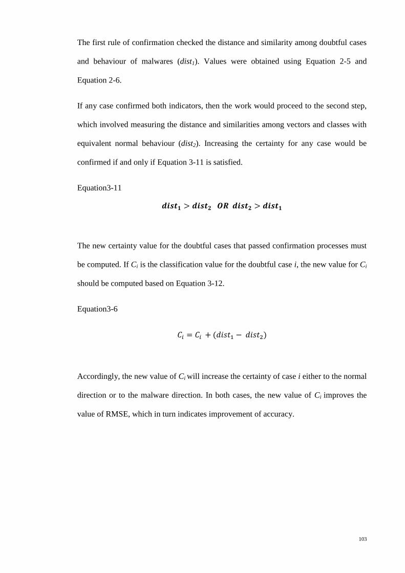
103

The first rule of confirmation checked the distance and similarity among doubtful cases

and behaviour of malwares (dist1). Values were obtained using Equation 2-5 and

Equation 2-6.

If any case confirmed both indicators, then the work would proceed to the second step,

which involved measuring the distance and similarities among vectors and classes with

equivalent normal behaviour (dist2). Increasing the certainty for any case would be

confirmed if and only if Equation 3-11 is satisfied.

Equation 3-11

The new certainty value for the doubtful cases that passed confirmation processes must

be computed. If Ci is the classification value for the doubtful case i, the new value for Ci

should be computed based on Equation 3-12.

Equation 3-6

( )

Accordingly, the new value of Ci will increase the certainty of case i either to the normal

direction or to the malware direction. In both cases, the new value of Ci improves the

value of RMSE, which in turn indicates improvement of accuracy.

104

3.6 Model‎and‎Problem’s‎Validation

A part of the present methodology is to validate ACC model against the important

theories and techniques that frequently employed as malicious API call classifier

models. This validation process that depends on some tests should confirm to facts:

1- Errors exist in the current classifier models due to characteristics similarity

of vectors that belongs to different classes.

2- Result of ACC model should show better accuracy results than other models.

In general, most studies depended on three types of techniques to achieve API call

classification. These techniques were either supervised or unsupervised AI algorithms,

or they followed some statistical theories. Therefore, this work tests the collected API

calls using the following AI techniques and statistical theories.

1- Supervised learning algorithm

a. Neural Network

b. Support Vector Machine

2- Unsupervised learning algorithm

a. SOM

b. K-mean clustering

3- Statistical theories: These theories depend mostly on computing the frequency or

probability of suspected API functions that mostly called by normal and rarely

called by malware application.

Results of these tests are shown in Table 5-4

105

3.7 Chapter Summary

This chapter explains the methodology steps of the ACC model as below:

1- ACC model is proposed by this work as a malicious API calls classifier models.

2- ACC model has three main parts. Each part has different sub-parts or steps.

3- Parts of the ACC model, mainly, related to:

a. Sample collection and API call vectors preparation. This part started by

collecting PE samples from different sources and ended by generating

two different patterns of API call vectors.

b. Designing an ANN as a classifier model, and using the two different data

sets of (1.a) as inputs for training and testing the ANN classifier model.

This part also results Signal-1 and Signal-2 at output.

c. Making a compression between results in Signal-1 and Signal-2.

Through this step, ACC model should be able to increase the certainty of

doubtful and misclassified results.

4- Clamping the same input data set (1.a) to some important classifier models, and

compare their results with the results that obtained by ACC model.

5- Some new ideas presented though this chapter, such as proposing new function

as a threshold value system. The new threshold value should support classifier

models better than the valid one.

106

Chapter 4

4- ACC Implementation

4.1 Introduction:

This chapter explains the implementation part of the ACC model. Through this chapter,

the three main parts of ACC model are executed individually. Moreover, details about

steps inside each main part are also explained. The first section of this chapter describes

the type and the version of softwares that employed by this work as well as the details

about OS environment where implementations are taken place.

As there are many techniques and theories involved in ACC model, this chapter also

covered information about parameters and features of the involved theories with regard

to the API call classifier models. More figures and tables are presented in this chapter to

explain the implementation process or to support the ACC methodology.

107

4.2 System environment and Employed Software

This work has executed all codes and PE samples using the Windows 7 OS. An HP

desktop computer with the following details was used:

· Model: HP Compaq dc7900 Convertible Minitower.

· Processor: Intel(R) Core(TM)2 Duo CPU E8400 @3.00GHz 3.00 GHz

· Memory (RAM): 4.00 GB

· System Type: Windows 7, 32 bit Operating System.

Three types of softwares are used in this work for coding and evaluation as follows:

· Matlab 2010b. Matlab software version 2010b was used throughout the work,

from coding most parts of the ACC model to code and test most classifier

models. To present and display the results, our work mostly depended on the

graphical tools of Matlab.

· SPSS Version 18. SPSS Version 18, statistical software that can perform most

statistical theories, was used in obtaining the frequency and probability of each

API function that might be called by any PE sample. The software even used

during model’s evaluation.

· The monitoring softwares have been used for extracting API functions that

called by PE samples. Two types of these softwares are employed. The first

software is called APIMonitoring (Version 2007) and the second is PE-Explorer

that is usable for Windows 7 (2008). Both softwares work only with Win 32-bit

PE files.

108

4.3 ACC Implementation: Part One

The following steps are needed to be achieved throughout the implementation of part

one of the ACC model. This part was introduced in chapter (3) as a sample collection

and API call vectors preparation. This part is started by specifying the characteristics of

PE samples that focused by this work and ended with generating to different patterns of

input dataset. Implementation details of each step in this part are explained in later

sections, wherever is necessary.

4.3.1 Properties of PE Samples

The wok introduced the properties of the required samples in section 3.3.1. The section

has focused only on the characteristics and properties of the malware and normal

applications that should be collected. The section also identified the type of malware

and normal applications that should be focused by this work. Furthermore, the section

also presented the justifications about each focused property.

The only aim of this section was to know the type of malwares and normal samples that

should be collected. Through sections 1.7, 2.6, and 3.3.1 all information regarding

samples and other relevant issues has been clearly identified. It has been decided

through these sections that the type of application which should be focused by this work

is PE structures.

As the aim for the section 3.3.1 was only to explain the properties of samples, therefore,

there is no coding works for this section. The only step that could be done here is to

move to the next section to find out the process that used by this work to identify

sources where samples could be found.

.

109

4.3.2 The sources of PE Samples

All sample properties that identified through section 3.3.1 have been passed to section

3.3.2 to guide the research how to find the required samples. Therefore, the aim of

section 3.3.2 was to find out where these samples could be obtained.

Through reviewing many researches, the work has found the possible ways that could

be followed to get malware and normal samples. Regarding normal samples, it was not

difficult to find them as most researches depended on applications from a fresh installed

Windows (H. D. Huang, Lee, Kao, Tsai, & Chang, 2011). However, obtained malware

samples were difficult. The ways that used by most researches are either downloading

them from online sources or capturing them through using Honeypot systems. Getting

malwares from other researchers was more difficult.

Here, this work wants to refer the Appendix-1 that contains valuable suggestions and

recommendations from a great malware analyst and a security architect from Symantec

Security Response, Mr. Peter Szor, regarding collecting malware samples. This work

decided to download PE malware samples from three different websites that mentioned

in section 3.3.1, based on these suggestions.

To decide how many samples are adequate for this research, the work has found in

(Parmjit Singh et al., 2009) that 500 samples are efficient for each type of applications

included in this work. As the work focused on four types of application (section 1.7),

therefore 2,000 samples are sufficient. However, because the section after 3.3.2 has

used to verify malware and normal samples, and there is a possibility that some samples

will not pass this verification process, therefore, this work decided to collect 10,000

malwares. As indicated in table 3-1, this work collected 3,500 PE Viruses, 3,500 PE

Trojan horses, and 3,000 PE Worms.

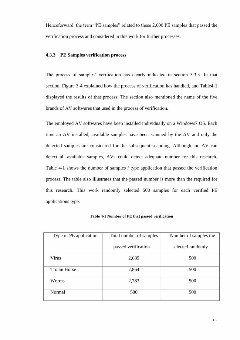
110

Henceforward, the term “PE samples” related to these 2,000 PE samples that passed the

verification process and considered in this work for further processes.

4.3.3 PE Samples verification process

The process of samples’ verification has clearly indicated in section 3.3.3. In that

section, Figure 3-4 explained how the process of verification has handled, and Table4-1

displayed the results of that process. The section also mentioned the name of the five

brands of AV softwares that used in the process of verification.

The employed AV softwares have been installed individually on a Windows7 OS. Each

time an AV installed, available samples have been scanned by the AV and only the

detected samples are considered for the subsequent scanning. Although, no AV can

detect all available samples, AVs could detect adequate number for this research.

Table 4-1 shows the number of samples / type application that passed the verification

process. The table also illustrates that the passed number is more than the required for

this research. This work randomly selected 500 samples for each verified PE

applications type.

Table ‎4-1 Number of PE that passed verification

Type of PE application Total number of samples

passed verification

Number of samples the

selected randomly

Virus 2,689 500

Trojan Horse 2,864 500

Worms 2,783 500

Normal 500 500

111

4.3.4 Extracting API Functions (Execution of PE samples):

PE samples under monitoring systems must be executed to extract the needed

information. Samples that passed verification processes in sections 3.3.3 and 4.3.3 were

executed under the APIMonitoring software. From this execution, the monitored

software can observe much information, including the name of each API function called

by the executed sample and the name of the DLL related to each API function.

The monitoring software reports the name of the API functions in the form of a name

sequence. The first name represents the first function called by the executed sample,

whereas the last name is the last necessary API function needed by the sample. The

monitoring software can track the system calling for any executed application. Each call

is represented as execution behaviour for the monitored sample. Therefore, this work

monitored the sequence of the execution behaviour by monitoring the execution of

samples using the APIMonitoring software.

In addition to obtaining the sequence of API functions’ name or the names of the

execution behaviour, this work obtained more information from monitoring the

execution process, as summarised below:

1- The DLL files that most frequently called by the executed sample. This work has

found that most DLL files used by PE samples during calling of API functions

are:

a. Kernel.dll; 820 API functions were monitored;

b. User32.dll; 621 API functions were monitored; and

c. Advapi32.dll; 430 API functions were monitored.

2- The total number of calls made by all PE samples was 326,942. In this

monitoring scenario 1,871 API functions are monitored, however, only 342

functions were called by PE samples.

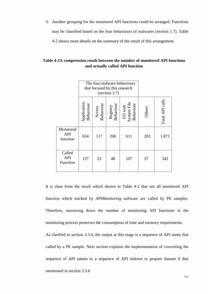
112

3- Another grouping for the monitored API functions could be arranged. Functions

may be classified based on the four behaviours of malwares (section 1.7). Table

4-2 shows more details on the summary of the result of this arrangement.

Table ‎4-2A compression result between the number of monitored API functions

and actually called API function

The four malware behaviours

that focused by this research

(section 1.7)

Appli

cati

on

Beh

avio

ur

Acc

ess

Beh

avio

ur

Reg

istr

y

Beh

avio

ur

I/O

wit

h

Syst

em F

ile

Beh

avio

ur

Oth

ers

Tota

l A

PI

call

s

Monitored

API

function 654 117 206 611 283 1,871

Called

API

Function 127 23 48 107 37 342

It is clear from the result which shown in Table 4-2 that not all monitored API

function which tracked by APIMonitoring software are called by PE samples.

Therefore, narrowing down the number of monitoring API functions in the

monitoring process preserves the consumption of time and memory requirements.

As clarified in section 3.3.4, the output at this stage is a sequence of API name that

called by a PE sample. Next section explains the implementation of converting the

sequence of API names to a sequence of API indexes to prepare dataset X that

mentioned in section 3.3.6

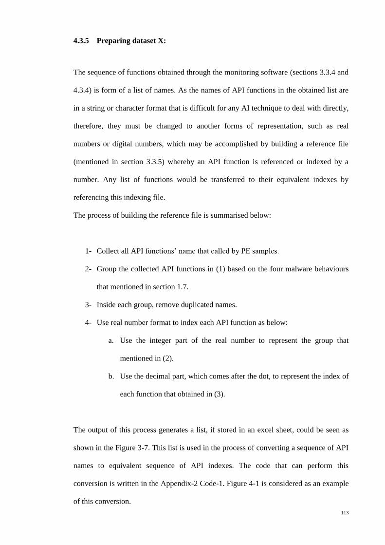
113

4.3.5 Preparing dataset X:

The sequence of functions obtained through the monitoring software (sections 3.3.4 and

4.3.4) is form of a list of names. As the names of API functions in the obtained list are

in a string or character format that is difficult for any AI technique to deal with directly,

therefore, they must be changed to another forms of representation, such as real

numbers or digital numbers, which may be accomplished by building a reference file

(mentioned in section 3.3.5) whereby an API function is referenced or indexed by a

number. Any list of functions would be transferred to their equivalent indexes by

referencing this indexing file.

The process of building the reference file is summarised below:

1- Collect all API functions’ name that called by PE samples.

2- Group the collected API functions in (1) based on the four malware behaviours

that mentioned in section 1.7.

3- Inside each group, remove duplicated names.

4- Use real number format to index each API function as below:

a. Use the integer part of the real number to represent the group that

mentioned in (2).

b. Use the decimal part, which comes after the dot, to represent the index of

each function that obtained in (3).

The output of this process generates a list, if stored in an excel sheet, could be seen as

shown in the Figure 3-7. This list is used in the process of converting a sequence of API

names to equivalent sequence of API indexes. The code that can perform this

conversion is written in the Appendix-2 Code-1. Figure 4-1 is considered as an example

of this conversion.

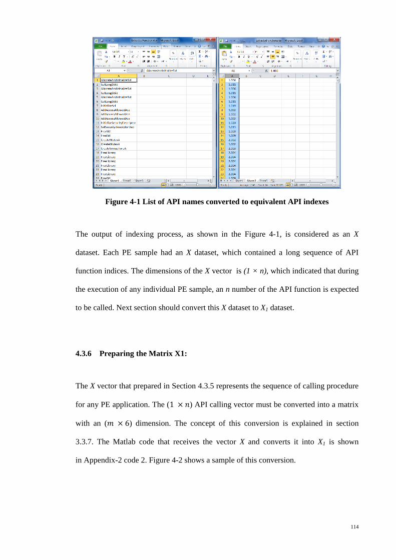
114

Figure ‎4-1 List of API names converted to equivalent API indexes

The output of indexing process, as shown in the Figure 4-1, is considered as an X

dataset. Each PE sample had an X dataset, which contained a long sequence of API

function indices. The dimensions of the X vector is (1 × n), which indicated that during

the execution of any individual PE sample, an n number of the API function is expected

to be called. Next section should convert this X dataset to X1 dataset.

4.3.6 Preparing the Matrix X1:

The X vector that prepared in Section 4.3.5 represents the sequence of calling procedure

for any PE application. The ( ) API calling vector must be converted into a matrix

with an ( ) dimension. The concept of this conversion is explained in section

3.3.7. The Matlab code that receives the vector X and converts it into X1 is shown

in Appendix-2 code 2. Figure 4-2 shows a sample of this conversion.

115

Figure ‎4-2 Sample of X to X1 conversion

After converting the sequence of each application that comes within the PE samples,

this work puts X1 vectors for all application in one set together. Assembling all X1

vectors in one set created a big X1 matrix with (25,319) vectors. However, (793)

duplicated vectors have been recorded, which means (793) duplicated behaviours in the

matrix.

In later section, this work uses X1 to train an ANN classifier model to distinguish

normal with malicious vectors. Existing duplicated vectors inside the training dataset

harms the training process of the ANN classifier model. Therefore, this work should

remove duplicated vectors in X1 dataset. After cleaning the X1 dataset from duplication,

only (24,526) unique vectors have been remained and considered for further process in

later sections.

In the next section, this work explains how the vector X is used to prepare the matrix X2.

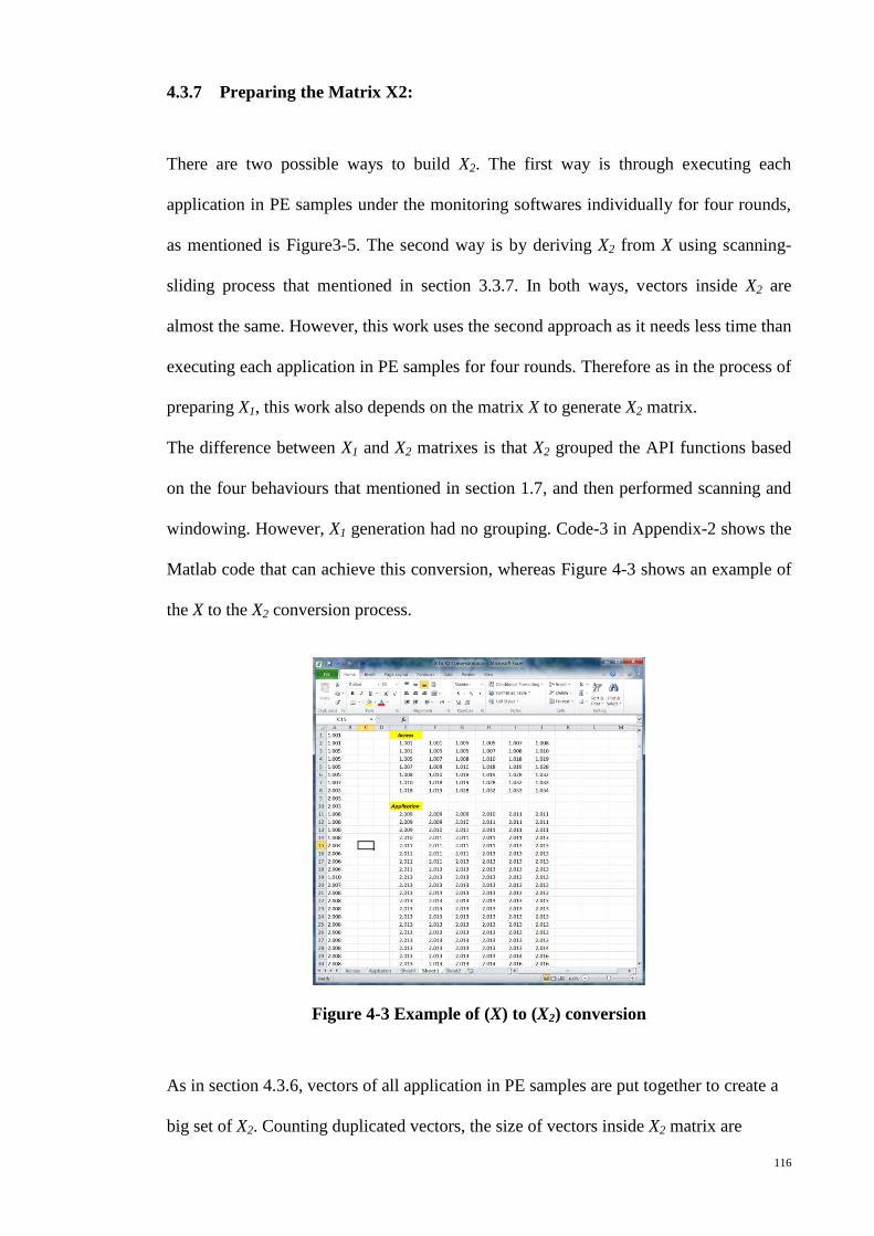
116

4.3.7 Preparing the Matrix X2:

There are two possible ways to build X2. The first way is through executing each

application in PE samples under the monitoring softwares individually for four rounds,

as mentioned is Figure3-5. The second way is by deriving X2 from X using scanning-

sliding process that mentioned in section 3.3.7. In both ways, vectors inside X2 are

almost the same. However, this work uses the second approach as it needs less time than

executing each application in PE samples for four rounds. Therefore as in the process of

preparing X1, this work also depends on the matrix X to generate X2 matrix.

The difference between X1 and X2 matrixes is that X2 grouped the API functions based

on the four behaviours that mentioned in section 1.7, and then performed scanning and

windowing. However, X1 generation had no grouping. Code-3 in Appendix-2 shows the

Matlab code that can achieve this conversion, whereas Figure 4-3 shows an example of

the X to the X2 conversion process.

Figure ‎4-3 Example of (X) to (X2) conversion

As in section 4.3.6, vectors of all application in PE samples are put together to create a

big set of X2. Counting duplicated vectors, the size of vectors inside X2 matrix are

117

(6,074). However, this number has reduced to (5,451) vectors after removing duplicated

vectors. Finally and before passing X1 and X2 to the part two of ACC model, vectors

inside these two dataset should be labelled as normal or malwares. The process of

labelling is clearly explained in section 3.3.8

4.4 Part TWO of ACC Model:

The main target of this part of the ACC model is to classify vectors that have a

dimension of (1 x 6) elements. This part receives such vectors from both X1 and X2

matrixes that prepared in sections 4.3.6 and 4.3.7.

As mentioned in sections 3.4.1 and 3.4.2, this part employed an ANN to classify each

clamped vectors to either normal or malware. In section 2.11.1, this work mentioned

that ANN classifier model has depended on Feed-forward Back Propagation as a

training algorithm.

Both X1 and X2 data set has been assigned to train and test the ANN classifier models in

two different phases. ANN with X1 has learned to distinguish a sequence of API indexes

that behaved normally with the one that behaved maliciously. However, X2 can train

ANN to distinguish four major behaviours (section 1.7) of PE malwares. ANN can learn

differently from X1 and X2, as the patterns of API calling sequences in these two dataset

are different. API sequences that kept inside X1 represent the general execution of a

suspected application, while sequences in X2 represent four major behaviours that

malwares more frequently follow (Section 3.3.1).

In this part, a new idea presents by this work to control misclassified and low certainty

classified cases. The new approach proposes a threshold value system that can map

results of ANN classifier models in to three areas; normal, malware, and doubtful areas.

Next section shows the process of training and testing the ANN classifier model using

X1 dataset.

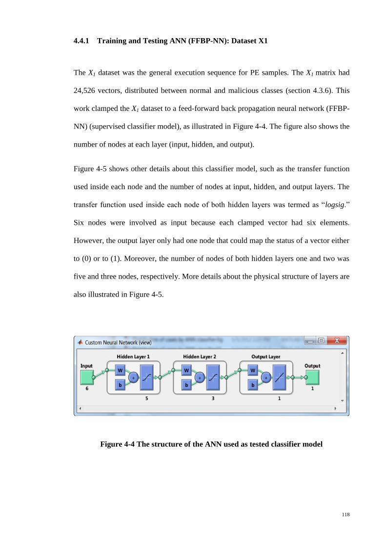
118

4.4.1 Training and Testing ANN (FFBP-NN): Dataset X1

The X1 dataset was the general execution sequence for PE samples. The X1 matrix had

24,526 vectors, distributed between normal and malicious classes (section 4.3.6). This

work clamped the X1 dataset to a feed-forward back propagation neural network (FFBP-

NN) (supervised classifier model), as illustrated in Figure 4-4. The figure also shows the

number of nodes at each layer (input, hidden, and output).

Figure 4-5 shows other details about this classifier model, such as the transfer function

used inside each node and the number of nodes at input, hidden, and output layers. The

transfer function used inside each node of both hidden layers was termed as “logsig.”

Six nodes were involved as input because each clamped vector had six elements.

However, the output layer only had one node that could map the status of a vector either

to (0) or to (1). Moreover, the number of nodes of both hidden layers one and two was

five and three nodes, respectively. More details about the physical structure of layers are

also illustrated in Figure 4-5.

Figure ‎4-4 The structure of the ANN used as tested classifier model

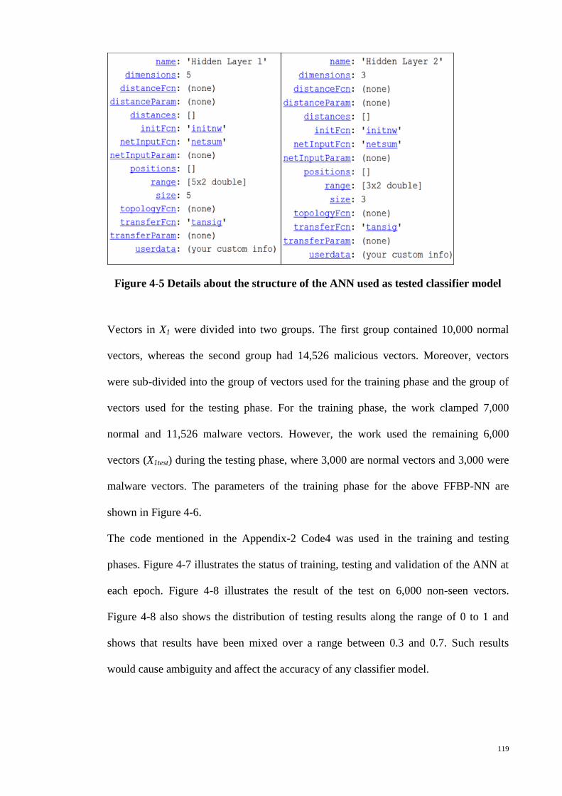
119

Figure ‎4-5 Details about the structure of the ANN used as tested classifier model

Vectors in X1 were divided into two groups. The first group contained 10,000 normal

vectors, whereas the second group had 14,526 malicious vectors. Moreover, vectors

were sub-divided into the group of vectors used for the training phase and the group of

vectors used for the testing phase. For the training phase, the work clamped 7,000

normal and 11,526 malware vectors. However, the work used the remaining 6,000

vectors (X1test) during the testing phase, where 3,000 are normal vectors and 3,000 were

malware vectors. The parameters of the training phase for the above FFBP-NN are

shown in Figure 4-6.

The code mentioned in the Appendix-2 Code4 was used in the training and testing

phases. Figure 4-7 illustrates the status of training, testing and validation of the ANN at

each epoch. Figure 4-8 illustrates the result of the test on 6,000 non-seen vectors.

Figure 4-8 also shows the distribution of testing results along the range of 0 to 1 and

shows that results have been mixed over a range between 0.3 and 0.7. Such results

would cause ambiguity and affect the accuracy of any classifier model.

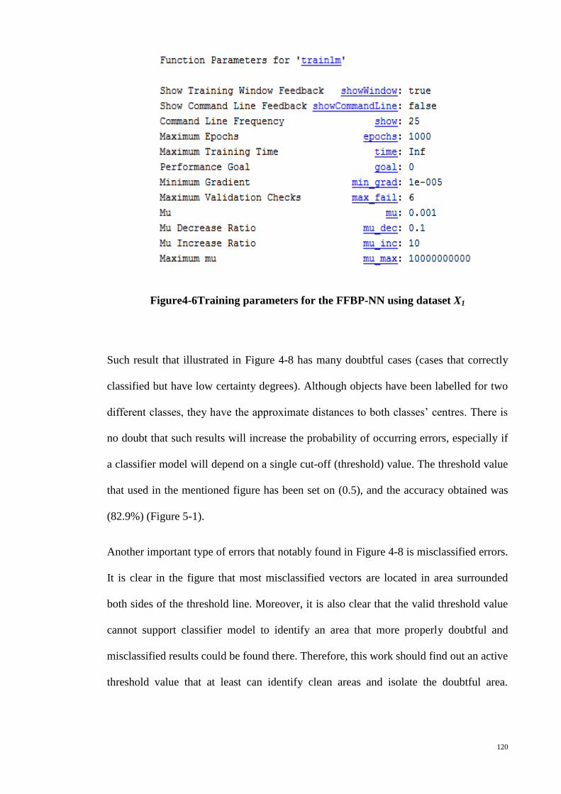
120

Figure‎4-6Training parameters for the FFBP-NN using dataset X1

Such result that illustrated in Figure 4-8 has many doubtful cases (cases that correctly

classified but have low certainty degrees). Although objects have been labelled for two

different classes, they have the approximate distances to both classes’ centres. There is

no doubt that such results will increase the probability of occurring errors, especially if

a classifier model will depend on a single cut-off (threshold) value. The threshold value

that used in the mentioned figure has been set on (0.5), and the accuracy obtained was

(82.9%) (Figure 5-1).

Another important type of errors that notably found in Figure 4-8 is misclassified errors.

It is clear in the figure that most misclassified vectors are located in area surrounded

both sides of the threshold line. Moreover, it is also clear that the valid threshold value

cannot support classifier model to identify an area that more properly doubtful and

misclassified results could be found there. Therefore, this work should find out an active

threshold value that at least can identify clean areas and isolate the doubtful area.

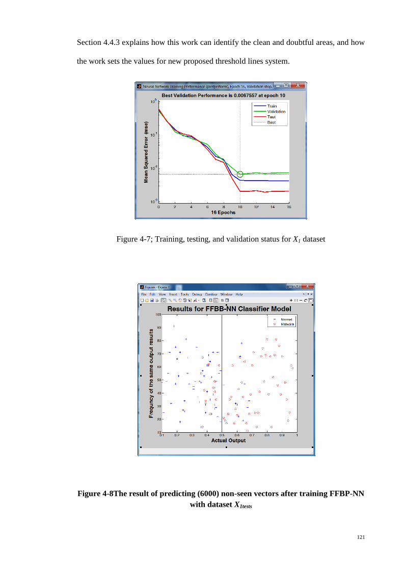
121

Section 4.4.3 explains how this work can identify the clean and doubtful areas, and how

the work sets the values for new proposed threshold lines system.

Figure 4-7; Training, testing, and validation status for X1 dataset

Figure ‎4-8The result of predicting (6000) non-seen vectors after training FFBP-NN

with dataset X1tests

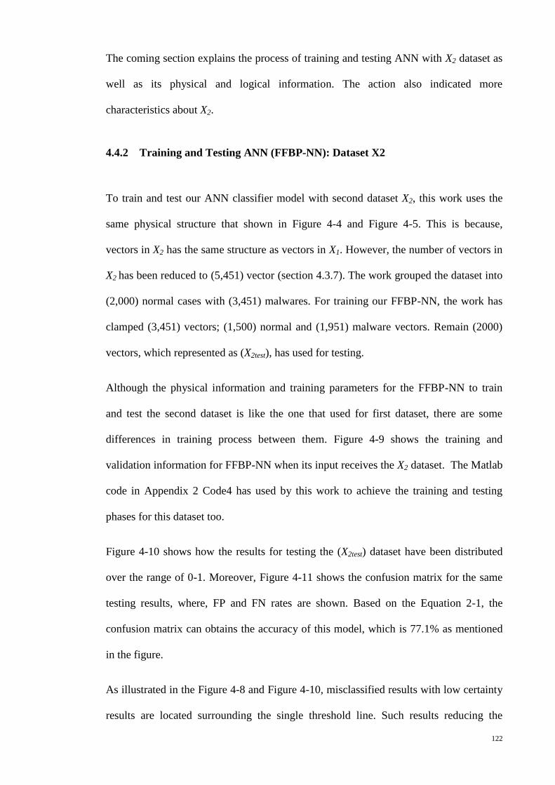
122

The coming section explains the process of training and testing ANN with X2 dataset as

well as its physical and logical information. The action also indicated more

characteristics about X2.

4.4.2 Training and Testing ANN (FFBP-NN): Dataset X2

To train and test our ANN classifier model with second dataset X2, this work uses the

same physical structure that shown in Figure 4-4 and Figure 4-5. This is because,

vectors in X2 has the same structure as vectors in X1. However, the number of vectors in

X2 has been reduced to (5,451) vector (section 4.3.7). The work grouped the dataset into

(2,000) normal cases with (3,451) malwares. For training our FFBP-NN, the work has

clamped (3,451) vectors; (1,500) normal and (1,951) malware vectors. Remain (2000)

vectors, which represented as (X2test), has used for testing.

Although the physical information and training parameters for the FFBP-NN to train

and test the second dataset is like the one that used for first dataset, there are some

differences in training process between them. Figure 4-9 shows the training and

validation information for FFBP-NN when its input receives the X2 dataset. The Matlab

code in Appendix 2 Code4 has used by this work to achieve the training and testing

phases for this dataset too.

Figure 4-10 shows how the results for testing the (X2test) dataset have been distributed

over the range of 0-1. Moreover, Figure 4-11 shows the confusion matrix for the same

testing results, where, FP and FN rates are shown. Based on the Equation 2-1, the

confusion matrix can obtains the accuracy of this model, which is 77.1% as mentioned

in the figure.

As illustrated in the Figure 4-8 and Figure 4-10, misclassified results with low certainty

results are located surrounding the single threshold line. Such results reducing the

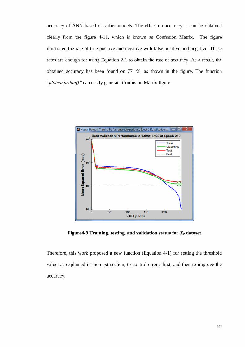
123

accuracy of ANN based classifier models. The effect on accuracy is can be obtained

clearly from the figure 4-11, which is known as Confusion Matrix. The figure

illustrated the rate of true positive and negative with false positive and negative. These

rates are enough for using Equation 2-1 to obtain the rate of accuracy. As a result, the

obtained accuracy has been found on 77.1%, as shown in the figure. The function

“plotconfusion()” can easily generate Confusion Matrix figure.

Figure‎4-9 Training, testing, and validation status for X2 dataset

Therefore, this work proposed a new function (Equation 4-1) for setting the threshold

value, as explained in the next section, to control errors, first, and then to improve the

accuracy.

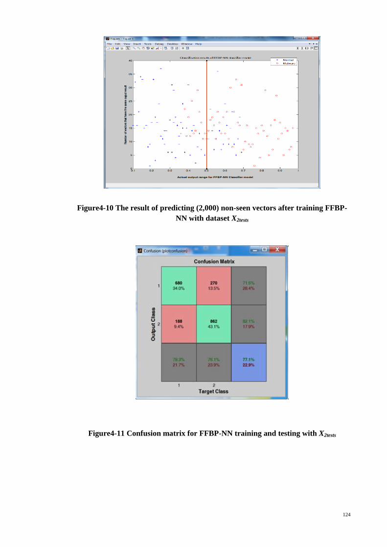
124

Figure‎4-10 The result of predicting (2,000) non-seen vectors after training FFBP-

NN with dataset X2tests

Figure‎4-11 Confusion matrix for FFBP-NN training and testing with X2tests

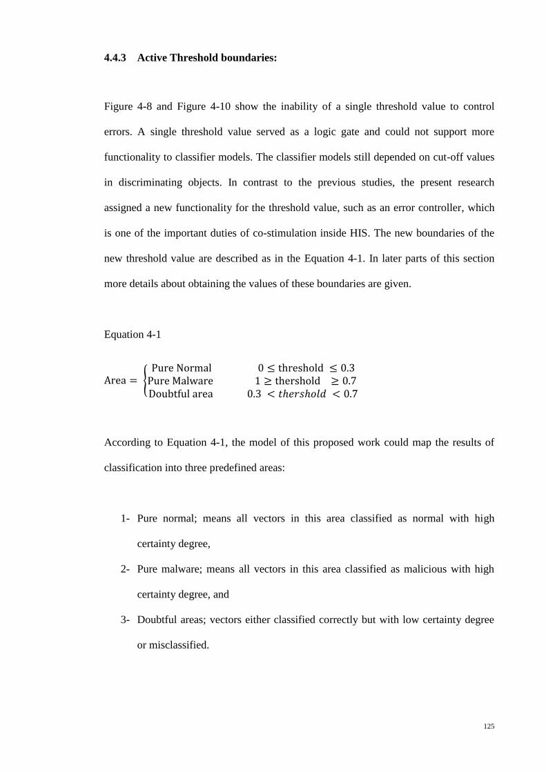
125

4.4.3 Active Threshold boundaries:

Figure 4-8 and Figure 4-10 show the inability of a single threshold value to control

errors. A single threshold value served as a logic gate and could not support more

functionality to classifier models. The classifier models still depended on cut-off values

in discriminating objects. In contrast to the previous studies, the present research

assigned a new functionality for the threshold value, such as an error controller, which

is one of the important duties of co-stimulation inside HIS. The new boundaries of the

new threshold value are described as in the Equation 4-1. In later parts of this section

more details about obtaining the values of these boundaries are given.

Equation 4-1

{

According to Equation 4-1, the model of this proposed work could map the results of

classification into three predefined areas:

1- Pure normal; means all vectors in this area classified as normal with high

certainty degree,

2- Pure malware; means all vectors in this area classified as malicious with high

certainty degree, and

3- Doubtful areas; vectors either classified correctly but with low certainty degree

or misclassified.

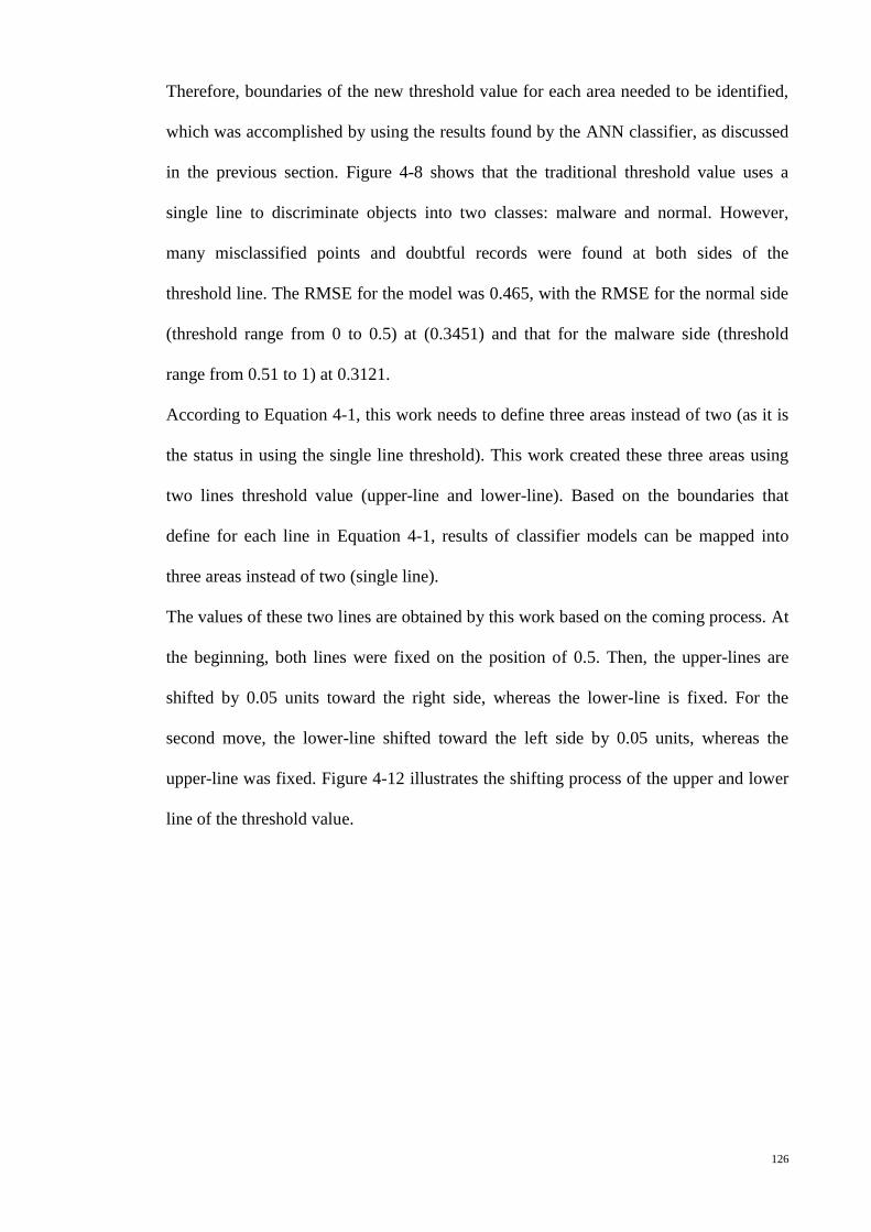
126

Therefore, boundaries of the new threshold value for each area needed to be identified,

which was accomplished by using the results found by the ANN classifier, as discussed

in the previous section. Figure 4-8 shows that the traditional threshold value uses a

single line to discriminate objects into two classes: malware and normal. However,

many misclassified points and doubtful records were found at both sides of the

threshold line. The RMSE for the model was 0.465, with the RMSE for the normal side

(threshold range from 0 to 0.5) at (0.3451) and that for the malware side (threshold

range from 0.51 to 1) at 0.3121.

According to Equation 4-1, this work needs to define three areas instead of two (as it is

the status in using the single line threshold). This work created these three areas using

two lines threshold value (upper-line and lower-line). Based on the boundaries that

define for each line in Equation 4-1, results of classifier models can be mapped into

three areas instead of two (single line).

The values of these two lines are obtained by this work based on the coming process. At

the beginning, both lines were fixed on the position of 0.5. Then, the upper-lines are

shifted by 0.05 units toward the right side, whereas the lower-line is fixed. For the

second move, the lower-line shifted toward the left side by 0.05 units, whereas the

upper-line was fixed. Figure 4-12 illustrates the shifting process of the upper and lower

line of the threshold value.

127

Figure ‎4-12 Shifting the threshold line process, and the THREE areas of results.

Within each shift, the work computes the RMSE for each defined area. The aim of these

tests is to find out the value of both threshold lines on which RMSE for each pure

normal and malware areas sets on a smallest value. Table 4-3 and Figure 4-13 show the

results that have been obtained during each shift. It is clear that value of RMSE in both

pure normal and pure malware areas are decreased within each shifting of threshold

value lines, while this value for the doubtful area is notably increased. With this

process, the work can create two cleaner areas and control the existing errors inside the

third one. The process of shifting lines will be continue until the value of RMSE in both

clean areas will not be decreasing notably. According to the Table 4-3 and Figure 4-13,

the work found that at test number nine and forward (where the value of upper line =

0.7 and the lower line = 0.3), the value of the RMSE, in all three areas, somehow

become fixed and the process of shifting lines no more affected them.

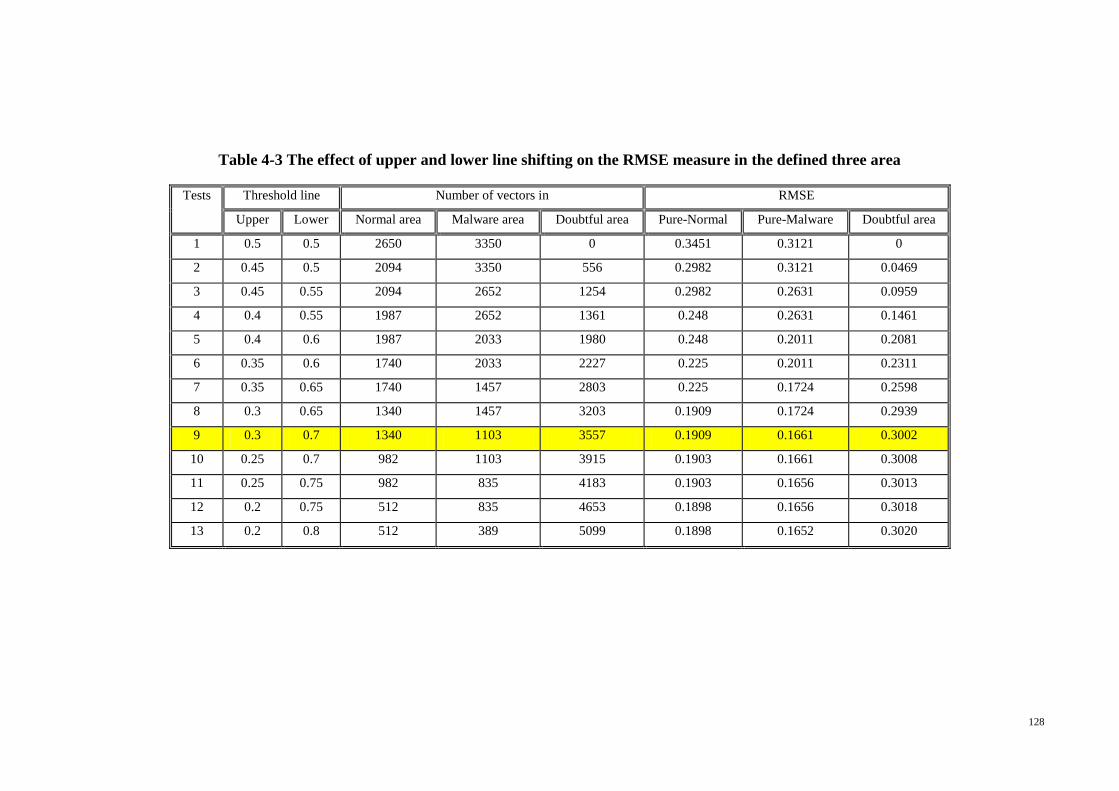
128

Table ‎4-3 The effect of upper and lower line shifting on the RMSE measure in the defined three area

Tests Threshold line Number of vectors in RMSE

Upper Lower Normal area Malware area Doubtful area Pure-Normal Pure-Malware Doubtful area

1 0.5 0.5 2650 3350 0 0.3451 0.3121 0

2 0.45 0.5 2094 3350 556 0.2982 0.3121 0.0469

3 0.45 0.55 2094 2652 1254 0.2982 0.2631 0.0959

4 0.4 0.55 1987 2652 1361 0.248 0.2631 0.1461

5 0.4 0.6 1987 2033 1980 0.248 0.2011 0.2081

6 0.35 0.6 1740 2033 2227 0.225 0.2011 0.2311

7 0.35 0.65 1740 1457 2803 0.225 0.1724 0.2598

8 0.3 0.65 1340 1457 3203 0.1909 0.1724 0.2939

9 0.3 0.7 1340 1103 3557 0.1909 0.1661 0.3002

10 0.25 0.7 982 1103 3915 0.1903 0.1661 0.3008

11 0.25 0.75 982 835 4183 0.1903 0.1656 0.3013

12 0.2 0.75 512 835 4653 0.1898 0.1656 0.3018

13 0.2 0.8 512 389 5099 0.1898 0.1652 0.3020

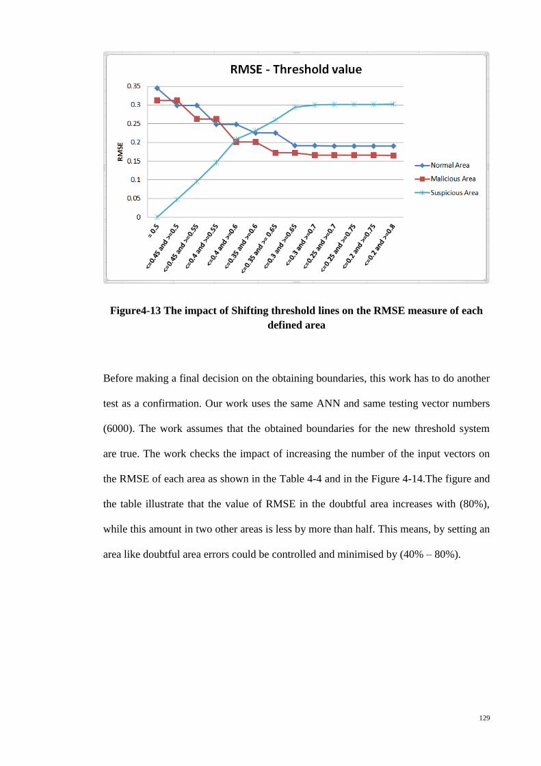
129

Figure‎4-13 The impact of Shifting threshold lines on the RMSE measure of each

defined area

Before making a final decision on the obtaining boundaries, this work has to do another

test as a confirmation. Our work uses the same ANN and same testing vector numbers

(6000). The work assumes that the obtained boundaries for the new threshold system

are true. The work checks the impact of increasing the number of the input vectors on

the RMSE of each area as shown in the Table 4-4 and in the Figure 4-14.The figure and

the table illustrate that the value of RMSE in the doubtful area increases with (80%),

while this amount in two other areas is less by more than half. This means, by setting an

area like doubtful area errors could be controlled and minimised by (40% – 80%).

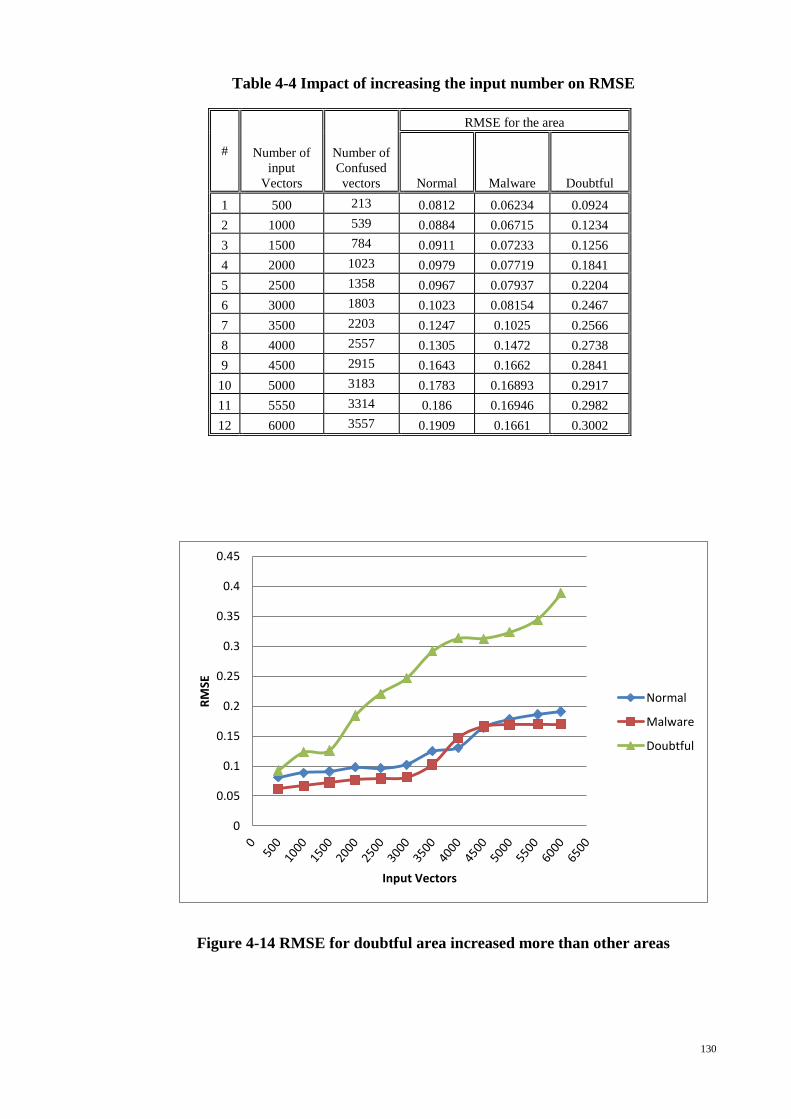
130

Table ‎4-4 Impact of increasing the input number on RMSE

# Number of

input

Vectors

Number of

Confused

vectors

RMSE for the area

Normal Malware Doubtful

1 500 213 0.0812 0.06234 0.0924

2 1000 539 0.0884 0.06715 0.1234

3 1500 784 0.0911 0.07233 0.1256

4 2000 1023 0.0979 0.07719 0.1841

5 2500 1358 0.0967 0.07937 0.2204

6 3000 1803 0.1023 0.08154 0.2467

7 3500 2203 0.1247 0.1025 0.2566

8 4000 2557 0.1305 0.1472 0.2738

9 4500 2915 0.1643 0.1662 0.2841

10 5000 3183 0.1783 0.16893 0.2917

11 5550 3314 0.186 0.16946 0.2982

12 6000 3557 0.1909 0.1661 0.3002

Figure ‎4-14 RMSE for doubtful area increased more than other areas

0

0.05

0.1

0.15

0.2

0.25

0.3

0.35

0.4

0.45

RM

SE

Input Vectors

Normal

Malware

Doubtful

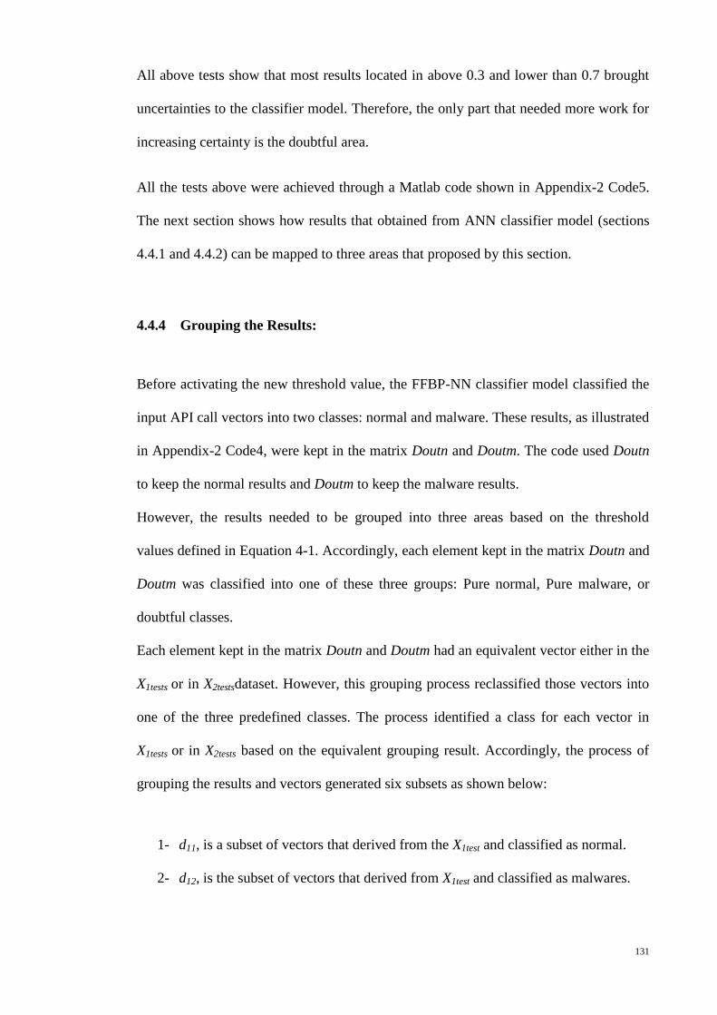
131

All above tests show that most results located in above 0.3 and lower than 0.7 brought

uncertainties to the classifier model. Therefore, the only part that needed more work for

increasing certainty is the doubtful area.

All the tests above were achieved through a Matlab code shown in Appendix-2 Code5.

The next section shows how results that obtained from ANN classifier model (sections

4.4.1 and 4.4.2) can be mapped to three areas that proposed by this section.

4.4.4 Grouping the Results:

Before activating the new threshold value, the FFBP-NN classifier model classified the

input API call vectors into two classes: normal and malware. These results, as illustrated

in Appendix-2 Code4, were kept in the matrix Doutn and Doutm. The code used Doutn

to keep the normal results and Doutm to keep the malware results.

However, the results needed to be grouped into three areas based on the threshold

values defined in Equation 4-1. Accordingly, each element kept in the matrix Doutn and

Doutm was classified into one of these three groups: Pure normal, Pure malware, or

doubtful classes.

Each element kept in the matrix Doutn and Doutm had an equivalent vector either in the

X1tests or in X2testsdataset. However, this grouping process reclassified those vectors into

one of the three predefined classes. The process identified a class for each vector in

X1tests or in X2tests based on the equivalent grouping result. Accordingly, the process of

grouping the results and vectors generated six subsets as shown below:

1- d11, is a subset of vectors that derived from the X1test and classified as normal.

2- d12, is the subset of vectors that derived from X1test and classified as malwares.

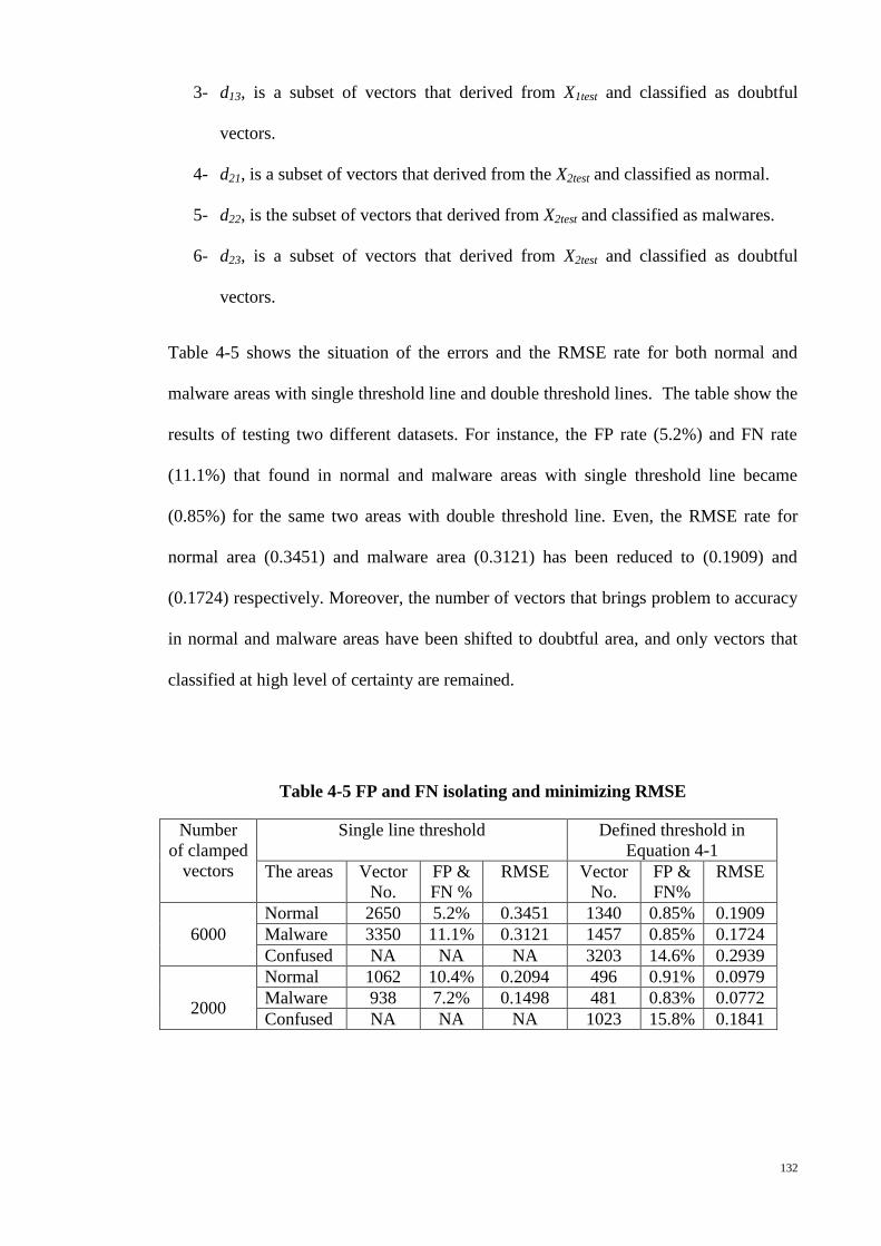
132

3- d13, is a subset of vectors that derived from X1test and classified as doubtful

vectors.

4- d21, is a subset of vectors that derived from the X2test and classified as normal.

5- d22, is the subset of vectors that derived from X2test and classified as malwares.

6- d23, is a subset of vectors that derived from X2test and classified as doubtful

vectors.

Table 4-5 shows the situation of the errors and the RMSE rate for both normal and

malware areas with single threshold line and double threshold lines. The table show the

results of testing two different datasets. For instance, the FP rate (5.2%) and FN rate

(11.1%) that found in normal and malware areas with single threshold line became

(0.85%) for the same two areas with double threshold line. Even, the RMSE rate for

normal area (0.3451) and malware area (0.3121) has been reduced to (0.1909) and

(0.1724) respectively. Moreover, the number of vectors that brings problem to accuracy

in normal and malware areas have been shifted to doubtful area, and only vectors that

classified at high level of certainty are remained.

Table ‎4-5 FP and FN isolating and minimizing RMSE

Number

of clamped

vectors

Single line threshold Defined threshold in

Equation 4-1

The areas Vector

No.

FP &

FN %

RMSE Vector

No.

FP &

FN%

RMSE

6000

Normal 2650 5.2% 0.3451 1340 0.85% 0.1909

Malware 3350 11.1% 0.3121 1457 0.85% 0.1724

Confused NA NA NA 3203 14.6% 0.2939

2000

Normal 1062 10.4% 0.2094 496 0.91% 0.0979

Malware 938 7.2% 0.1498 481 0.83% 0.0772

Confused NA NA NA 1023 15.8% 0.1841

133

Through this process, the work groups the doubtful and misclassified results into d13

and d23 groups. It means errors in both normal and malware classes can be isolated. This

work focused on the area that needed more improvement in the entire classification

accuracy. Therefore, in the next section this work uses a functionality of co-stimulation

to improve the accuracy of ANN classifier model by increase the certainty of low

certainty cases and reclassify the misclassified results.

4.5 Part THREE of ACC Model: Co-stimulation

The main target of this part is to increase the certainty degree of doubtfully classified

cases and reclassifies the misclassified cases. This improvement can be achieved

through a process named co-stimulation.

The process considered vectors inside d13 that contains high misclassified and

doubtfully classified vectors. The process also involved vectors in d21 and d22 that

contain high classified vectors with a few misclassified cases.

The process of co-stimulation can measure some similarity figures between a low

certainty vector in d13 with vectors in both d21 and d22together. Later, the process

considers the degree of similarity with the old certainty degree of the vector to compute

new and better certainty degree for the doubtful vector. Latter sections give more details

about co-stimulation process. However, the next section starts to find out indicators that

accordingly two vectors are considered as similar or non-similar through co-stimulation

process.

134

4.5.1 Calculating the Similarity Measurement

To define two vectors similar or non-similar, co-stimulation process needs define two

measures to evaluate the similarity degree between both vectors or between a vector and

a class. Both measures were extracted from the vectors classified as high certainty

vectors, that is, vectors kept in matrixes d11with d12fornormaland d21with d22formalware.

The work evaluated those vectors to determine two important indicators, which would

function as threshold values. The first indicator used to decide the similarity between

two vectors, whereas the second indicator can check the distance between vectors and

classes. Below steps show calculating process for the value of both indicators:

A- Identifying the value of the first indicator (When two vectors are similar):

1- Within a certain behaviour class, the similarity degree between each vector and

the remaining vectors would be computed. Afterward, the vector’s average

similarity (VAS) was obtained for each vector. If class A has n vectors, each

vector in class A has (n) similarity, and each vector should have one VAS.

However, class A should have (n) VAS.

2- For each class, the overall average similarity (OAS) would be computed

depending on the VAS of each vector (class A has only one OAS). The value of

OAS represents the value of the indicator used for evaluating the similarity

among vectors within a certain class.

3- Each behaviour class has different vectors and different number of vectors.

Hence, behaviour classes would have different values for their similarity

indicator.

4- Vectors are considered to be similar to any vector inside a certain behaviour

class if and only if their Cosine Similarity is equal to or greater than the OAS

value of that class.

135

B- Identifying the value of the second indicator (vector to class similarity):

1- Within a certain behaviour class and for each vector, the VAS of each vector

would be compared with the OAS values of that class. The number of vectors

(assume ) that has a VAS equal to or greater than the OAS of the class is

identified.

2- This work considered the value of as the second indicator value.

Accordingly, closer behaviour classes for doubtful vectors were identified if and only if

their VAS values were equal to or greater than the OAS value for a number of vectors

that can pass the number (test one or T1 or Signal-1). If a doubtful vector from a

malware behaviour class is identified, another confirmation test must be conducted,

namely, test two or T2 or Signal-2. The Signal-2 would test the same doubtful vector

with the normal behaviour class equivalent to the malware behaviour class, which was

identified through Signal-1. The conditions that should be satisfied through Signal-2

would be an inverse of the conditions applied through Signal-1.

Table 4-5 presents the figures used to compute both values of the indicators. The total

number of vectors in all matrixes normal and malwares was 3, 774 vectors: 1, 836 and

1, 938 normal and malware vectors, respectively. However, the 977 vectors that

belonged to the X2test dataset were sub classified based on four malware behaviours.

Figure 4-15 shows the numbers of high-certainty vectors in the main and sub classes of

the malware and normal datasets.

The code mentioned in the Appendix 2 – Code6 was used in archiving, collecting

information, and identifying both values of the indicators. Table 4-6 and Table 4-7

illustrate the obtained values for OAS and for all normal and malware behavior

classes.

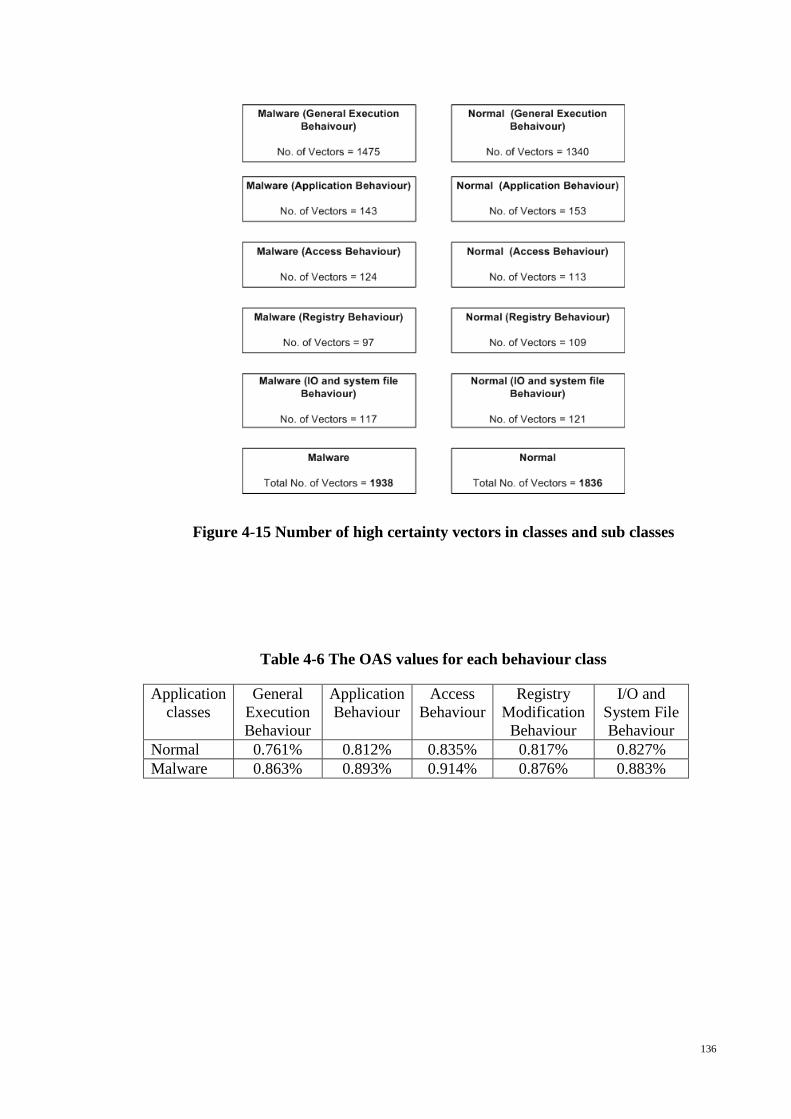
136

Figure ‎4-15 Number of high certainty vectors in classes and sub classes

Table ‎4-6 The OAS values for each behaviour class

Application

classes

General

Execution

Behaviour

Application

Behaviour

Access

Behaviour

Registry

Modification

Behaviour

I/O and

System File

Behaviour

Normal 0.761% 0.812% 0.835% 0.817% 0.827%

Malware 0.863% 0.893% 0.914% 0.876% 0.883%

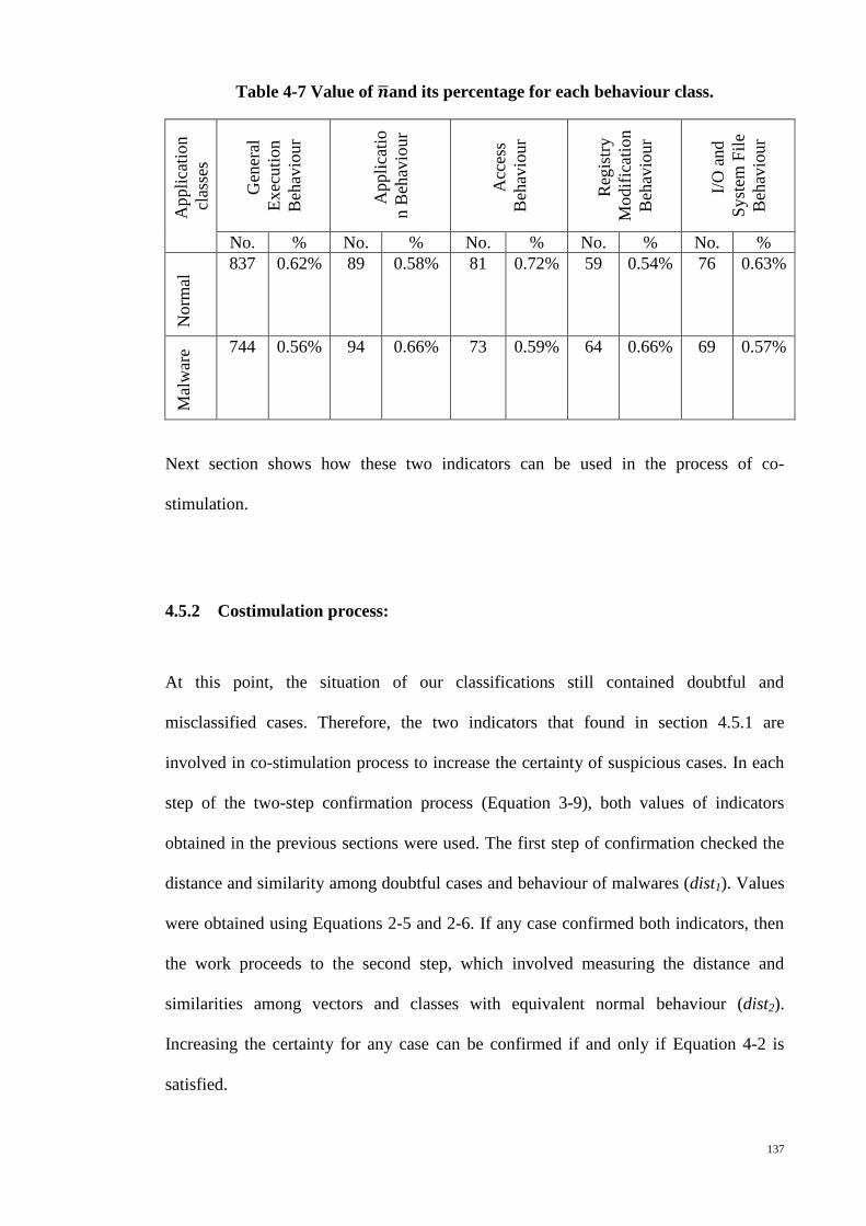
137

Table ‎4-7 Value of and its percentage for each behaviour class.

Appli

cati

on

clas

ses

Gen

eral

Exec

uti

on

Beh

avio

ur

Appli

cati

o

n B

ehav

iour

Acc

ess

Beh

avio

ur

Reg

istr

y

Modif

icat

ion

Beh

avio

ur

I/O

and

Syst

em F

ile

Beh

avio

ur

No. % No. % No. % No. % No. %

Norm

al 837 0.62% 89 0.58% 81 0.72% 59 0.54% 76 0.63%

Mal

war

e 744 0.56% 94 0.66% 73 0.59% 64 0.66% 69 0.57%

Next section shows how these two indicators can be used in the process of co-

stimulation.

4.5.2 Costimulation process:

At this point, the situation of our classifications still contained doubtful and

misclassified cases. Therefore, the two indicators that found in section 4.5.1 are

involved in co-stimulation process to increase the certainty of suspicious cases. In each

step of the two-step confirmation process (Equation 3-9), both values of indicators

obtained in the previous sections were used. The first step of confirmation checked the

distance and similarity among doubtful cases and behaviour of malwares (dist1). Values

were obtained using Equations 2-5 and 2-6. If any case confirmed both indicators, then

the work proceeds to the second step, which involved measuring the distance and

similarities among vectors and classes with equivalent normal behaviour (dist2).

Increasing the certainty for any case can be confirmed if and only if Equation 4-2 is

satisfied.

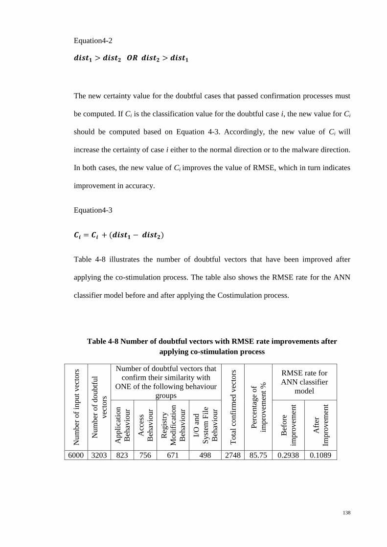
138

Equation 4-2

The new certainty value for the doubtful cases that passed confirmation processes must

be computed. If Ci is the classification value for the doubtful case i, the new value for Ci

should be computed based on Equation 4-3. Accordingly, the new value of Ci will

increase the certainty of case i either to the normal direction or to the malware direction.

In both cases, the new value of Ci improves the value of RMSE, which in turn indicates

improvement in accuracy.

Equation 4-3

( )

Table 4-8 illustrates the number of doubtful vectors that have been improved after

applying the co-stimulation process. The table also shows the RMSE rate for the ANN

classifier model before and after applying the Costimulation process.

Table ‎4-8 Number of doubtful vectors with RMSE rate improvements after

applying co-stimulation process

Num

ber

of

input

vec

tors

Num

ber

of

doubtf

ul

vec

tors

Number of doubtful vectors that

confirm their similarity with

ONE of the following behaviour

groups

Tota

l co

nfi

rmed

vec

tors

Per

centa

ge

of

impro

vem

ent

%

RMSE rate for

ANN classifier

model

Appli

cati

on

Beh

avio

ur

Acc

ess

Beh

avio

ur

Reg

istr

y

Modif

icat

ion

Beh

avio

ur

I/O

and

Syst

em F

ile

Beh

avio

ur

Bef

ore

impro

vem

ent

Aft

er

Impro

vem

ent

6000 3203 823 756 671 498 2748 85.75 0.2938 0.1089

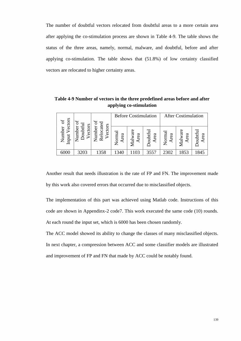
139

The number of doubtful vectors relocated from doubtful areas to a more certain area

after applying the co-stimulation process are shown in Table 4-9. The table shows the

status of the three areas, namely, normal, malware, and doubtful, before and after

applying co-stimulation. The table shows that (51.8%) of low certainty classified

vectors are relocated to higher certainty areas.

Table ‎4-9 Number of vectors in the three predefined areas before and after

applying co-stimulation

Num

ber

of

Input

Vec

tors

Num

ber

of

Doubtf

ul

Vec

tors

Num

ber

of

Rel

oca

ted

Vec

tors

Before Costimulation After Costimulation N

orm

al

Are

a

Mal

war

e

Are

a

Doubtf

ul

Are

a

Norm

al

Are

a

Mal

war

e

Are

a

Doubtf

ul

Are

a

6000 3203 1358 1340 1103 3557 2302 1853 1845

Another result that needs illustration is the rate of FP and FN. The improvement made

by this work also covered errors that occurred due to misclassified objects.

The implementation of this part was achieved using Matlab code. Instructions of this

code are shown in Appendinx-2 code7. This work executed the same code (10) rounds.

At each round the input set, which is 6000 has been chosen randomly.

The ACC model showed its ability to change the classes of many misclassified objects.

In next chapter, a compression between ACC and some classifier models are illustrated

and improvement of FP and FN that made by ACC could be notably found.

140

4.6 Chapter Summary

The implementation processes that described throughout the chapter four is summarized

as below:

1- This work has utilized the process of malware samples verification to avoid

possibility of finding any noises in malware’s samples.

2- It is not necessary for a PE application to call all API functions available inside

computer system. PE applications only need to call the API functions that

necessary for their execution.

3- The long sequence of API functions that called by an application could be

broken down to smaller parts of sequences, which each of them represent a

behaviour of the application during its execution.

4- For each type of application’s execution behaviour there is a concerned group of

API function. To monitor a specific behaviour of an application, tracing the

behaviour’s concerned group of API function is enough.

5- ANN is a good classifier model. However, it has many misclassified or doubtful

classified cases. Current threshold value that used with all classified models has

no ability to identify which area causes more errors that affect the accuracy.

6- The result of any classifier model could be divided into three areas; normal,

malware, and doubtful area.

7- This work needs to depend on some indicators in order to decide whether two

vectors are similar or not.

8- Process of co-stimulation is a confirmation of a case in two directions.

141

Chapter 5

5. Evaluating ACC with other Classifier models

5.1 Introduction

Although the tools and the techniques that employed by researchers for devising

classifier models were different, the concept and the algorithms that activated by them

were followed either supervised or unsupervised methods (Ando et al., 2009; Merkel et

al., 2010; Miao Wang, 2009; B. Zhang et al., 2006; Y. Zhang et al., 2010; H. Zhao et

al., 2009; Zou et al., 2009). Moreover, Statistical theories was another concept that

intended by researchers to build classifier models. Different statistical methods used by

researchers to measure the membership probability degree for an unknown case inside a

class. Measuring the frequency for a malware’s behaviour was another statistical

method (Cha, 2007).

Regarding the input dataset, researchers were clamped only one dataset as an input to

their systems. Therefore, this work tests some supervised and unsupervised detection

models depending only on the X1 dataset, which has (24,526) vectors. The work also

tested two concepts of statistical theories. Below are more details of the tested models:

1- Supervised learning methods.

a. Neural Network; Feed forward Back-Propagation algorithm

b. Support Vector Machine.

2- Unsupervised learning methods;

a. Neural Network: Self-Organizing Map.

b. K-means algorithm

3- Statistical Theory (Obtaining the frequently of function calling).

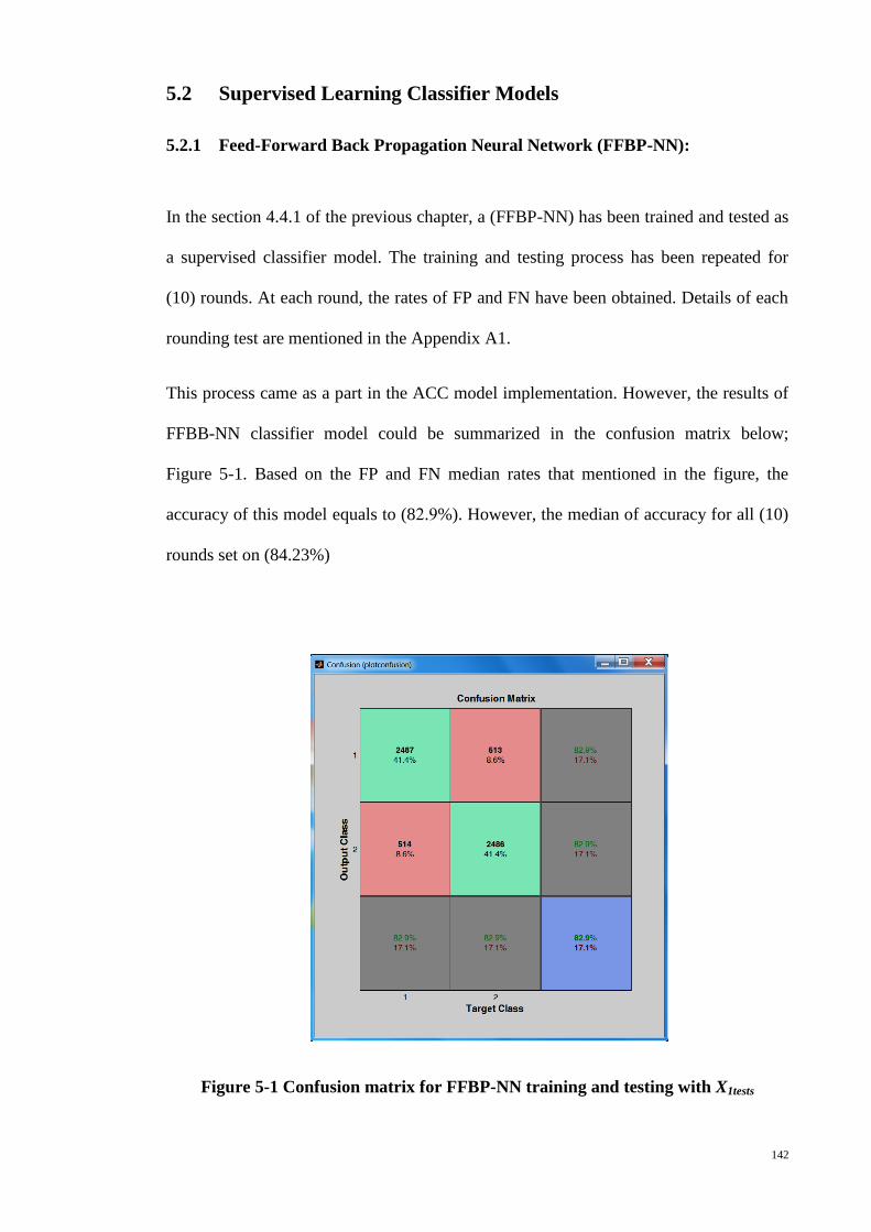
142

5.2 Supervised Learning Classifier Models

5.2.1 Feed-Forward Back Propagation Neural Network (FFBP-NN):

In the section 4.4.1 of the previous chapter, a (FFBP-NN) has been trained and tested as

a supervised classifier model. The training and testing process has been repeated for

(10) rounds. At each round, the rates of FP and FN have been obtained. Details of each

rounding test are mentioned in the Appendix A1.

This process came as a part in the ACC model implementation. However, the results of

FFBB-NN classifier model could be summarized in the confusion matrix below;

Figure 5-1. Based on the FP and FN median rates that mentioned in the figure, the

accuracy of this model equals to (82.9%). However, the median of accuracy for all (10)

rounds set on (84.23%)

Figure ‎5-1 Confusion matrix for FFBP-NN training and testing with X1tests

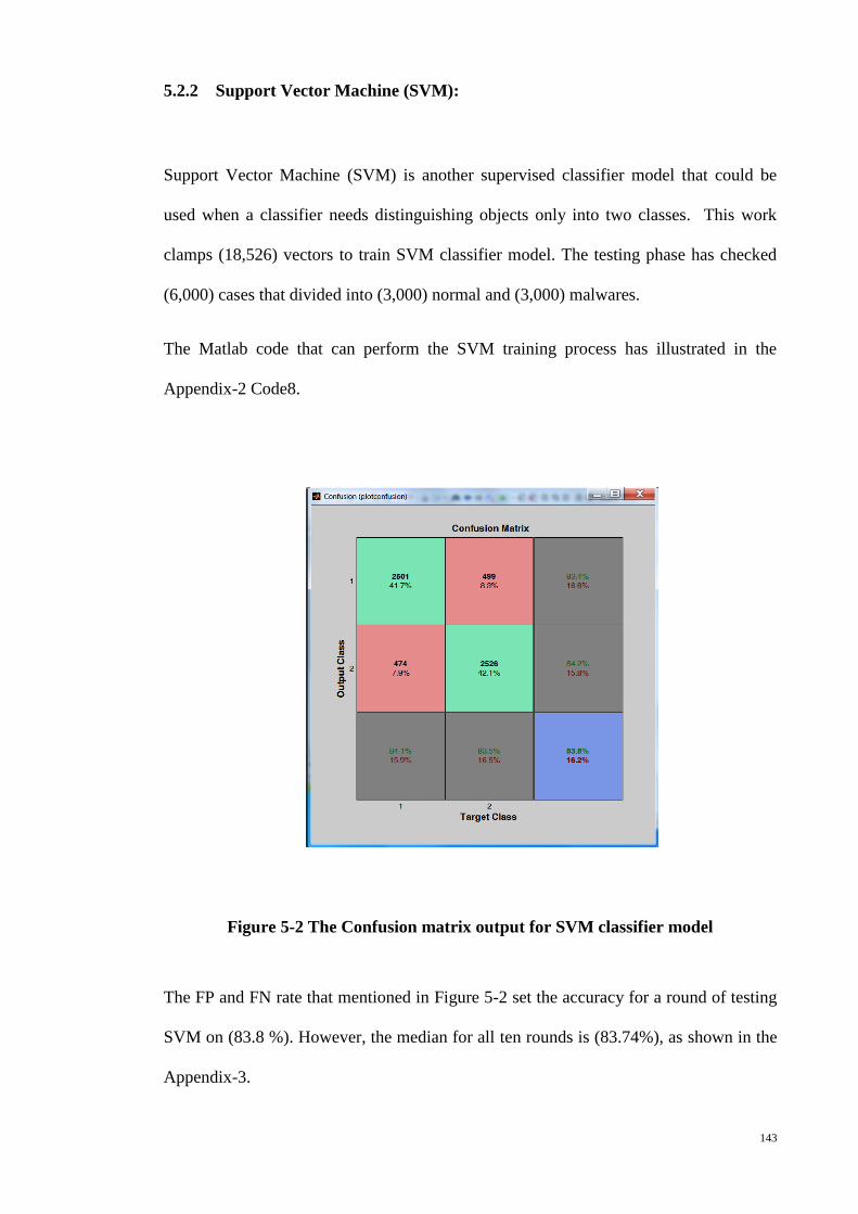
143

5.2.2 Support Vector Machine (SVM):

Support Vector Machine (SVM) is another supervised classifier model that could be

used when a classifier needs distinguishing objects only into two classes. This work

clamps (18,526) vectors to train SVM classifier model. The testing phase has checked

(6,000) cases that divided into (3,000) normal and (3,000) malwares.

The Matlab code that can perform the SVM training process has illustrated in the

Appendix-2 Code8.

Figure ‎5-2 The Confusion matrix output for SVM classifier model

The FP and FN rate that mentioned in Figure 5-2 set the accuracy for a round of testing

SVM on (83.8 %). However, the median for all ten rounds is (83.74%), as shown in the

Appendix-3.

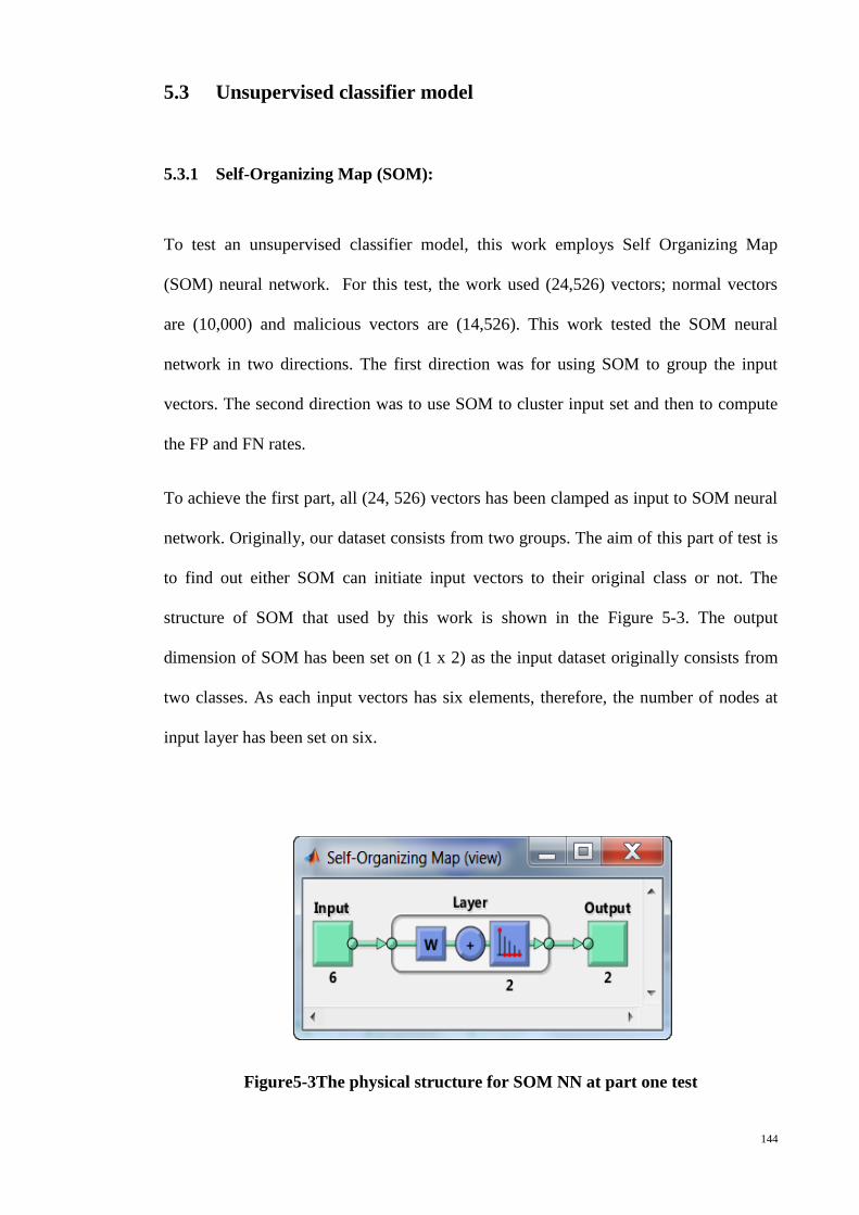
144

5.3 Unsupervised classifier model

5.3.1 Self-Organizing Map (SOM):

To test an unsupervised classifier model, this work employs Self Organizing Map

(SOM) neural network. For this test, the work used (24,526) vectors; normal vectors

are (10,000) and malicious vectors are (14,526). This work tested the SOM neural

network in two directions. The first direction was for using SOM to group the input

vectors. The second direction was to use SOM to cluster input set and then to compute

the FP and FN rates.

To achieve the first part, all (24, 526) vectors has been clamped as input to SOM neural

network. Originally, our dataset consists from two groups. The aim of this part of test is

to find out either SOM can initiate input vectors to their original class or not. The

structure of SOM that used by this work is shown in the Figure 5-3. The output

dimension of SOM has been set on (1 x 2) as the input dataset originally consists from

two classes. As each input vectors has six elements, therefore, the number of nodes at

input layer has been set on six.

Figure‎5-3The physical structure for SOM NN at part one test

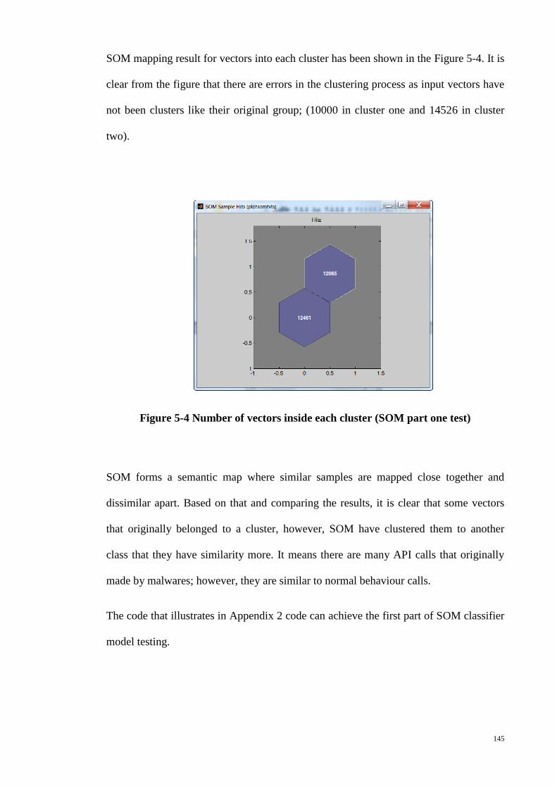
145

SOM mapping result for vectors into each cluster has been shown in the Figure 5-4. It is

clear from the figure that there are errors in the clustering process as input vectors have

not been clusters like their original group; (10000 in cluster one and 14526 in cluster

two).

Figure ‎5-4 Number of vectors inside each cluster (SOM part one test)

SOM forms a semantic map where similar samples are mapped close together and

dissimilar apart. Based on that and comparing the results, it is clear that some vectors

that originally belonged to a cluster, however, SOM have clustered them to another

class that they have similarity more. It means there are many API calls that originally

made by malwares; however, they are similar to normal behaviour calls.

The code that illustrates in Appendix 2 code can achieve the first part of SOM classifier

model testing.

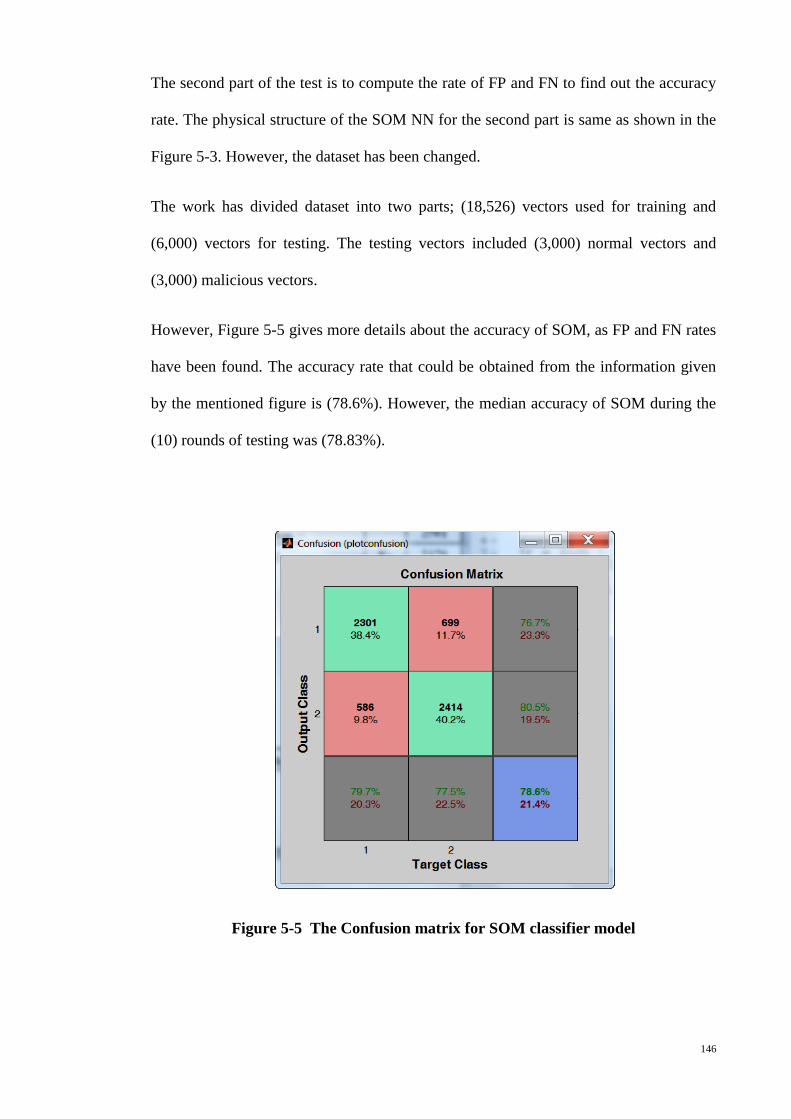
146

The second part of the test is to compute the rate of FP and FN to find out the accuracy

rate. The physical structure of the SOM NN for the second part is same as shown in the

Figure 5-3. However, the dataset has been changed.

The work has divided dataset into two parts; (18,526) vectors used for training and

(6,000) vectors for testing. The testing vectors included (3,000) normal vectors and

(3,000) malicious vectors.

However, Figure 5-5 gives more details about the accuracy of SOM, as FP and FN rates

have been found. The accuracy rate that could be obtained from the information given

by the mentioned figure is (78.6%). However, the median accuracy of SOM during the

(10) rounds of testing was (78.83%).

Figure ‎5-5 The Confusion matrix for SOM classifier model

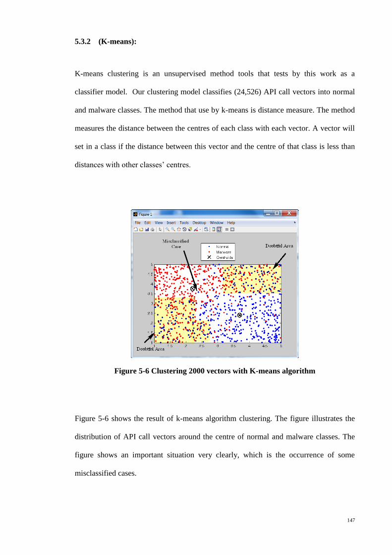
147

5.3.2 (K-means):

K-means clustering is an unsupervised method tools that tests by this work as a

classifier model. Our clustering model classifies (24,526) API call vectors into normal

and malware classes. The method that use by k-means is distance measure. The method

measures the distance between the centres of each class with each vector. A vector will

set in a class if the distance between this vector and the centre of that class is less than

distances with other classes’ centres.

Figure ‎5-6 Clustering 2000 vectors with K-means algorithm

Figure 5-6 shows the result of k-means algorithm clustering. The figure illustrates the

distribution of API call vectors around the centre of normal and malware classes. The

figure shows an important situation very clearly, which is the occurrence of some

misclassified cases.

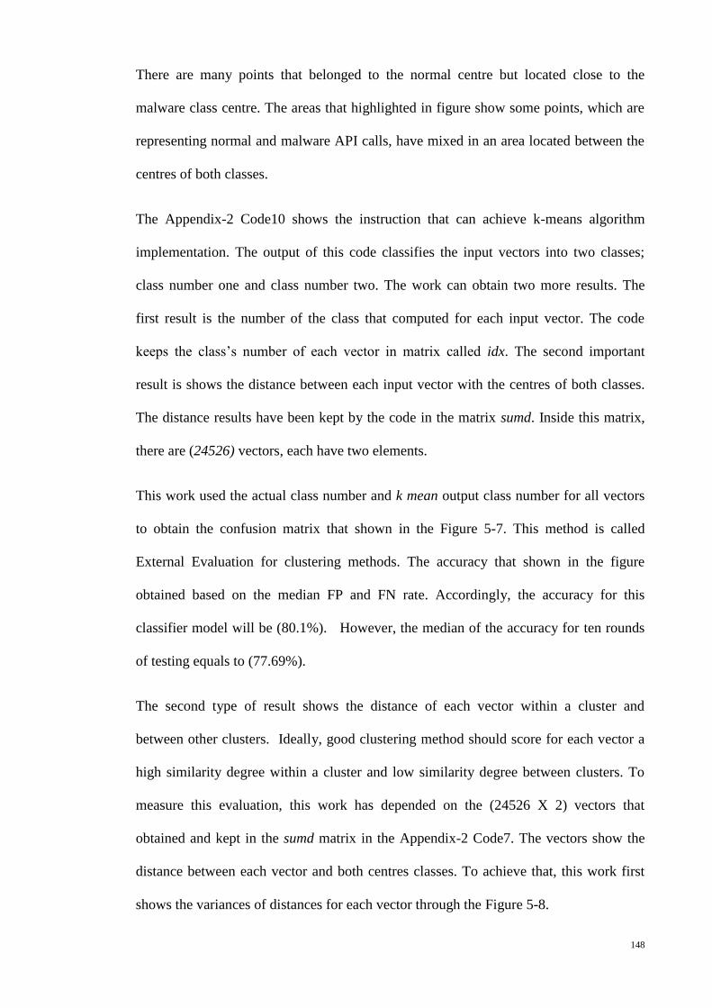
148

There are many points that belonged to the normal centre but located close to the

malware class centre. The areas that highlighted in figure show some points, which are

representing normal and malware API calls, have mixed in an area located between the

centres of both classes.

The Appendix-2 Code10 shows the instruction that can achieve k-means algorithm

implementation. The output of this code classifies the input vectors into two classes;

class number one and class number two. The work can obtain two more results. The

first result is the number of the class that computed for each input vector. The code

keeps the class’s number of each vector in matrix called idx. The second important

result is shows the distance between each input vector with the centres of both classes.

The distance results have been kept by the code in the matrix sumd. Inside this matrix,

there are (24526) vectors, each have two elements.

This work used the actual class number and k mean output class number for all vectors

to obtain the confusion matrix that shown in the Figure 5-7. This method is called

External Evaluation for clustering methods. The accuracy that shown in the figure

obtained based on the median FP and FN rate. Accordingly, the accuracy for this

classifier model will be (80.1%). However, the median of the accuracy for ten rounds

of testing equals to (77.69%).

The second type of result shows the distance of each vector within a cluster and

between other clusters. Ideally, good clustering method should score for each vector a

high similarity degree within a cluster and low similarity degree between clusters. To

measure this evaluation, this work has depended on the (24526 X 2) vectors that

obtained and kept in the sumd matrix in the Appendix-2 Code7. The vectors show the

distance between each vector and both centres classes. To achieve that, this work first

shows the variances of distances for each vector through the Figure 5-8.

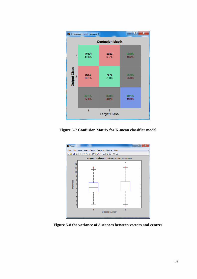
149

Figure ‎5-7 Confusion Matrix for K-mean classifier model

Figure ‎5-8 the variance of distances between vectors and centres

150

For both classes, it is clear that distances have been separated between 2 and 12, and the

mean of the distance for both classes is around 6. Now going back to distances that have

been kept in sumd, this work can obtain some measures as illustrated in Table5-1.

Table ‎5-1 Number of vectors inside and outside the mean distance for each class

Class’s Number Number of Distances > 6 Number of Distance < 6 Total number of vectors

Class 1 10,668 13,858 24,526

Class 2 9,216 15,310 24,526

It is clear from the table that many vectors are located outside the mean distance for

each class. The clustering certainty of such vectors is very low, which increases the rate

of RMSE.

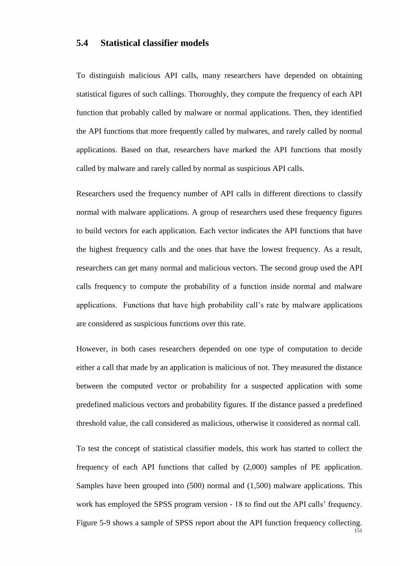
151

5.4 Statistical classifier models

To distinguish malicious API calls, many researchers have depended on obtaining

statistical figures of such callings. Thoroughly, they compute the frequency of each API

function that probably called by malware or normal applications. Then, they identified

the API functions that more frequently called by malwares, and rarely called by normal

applications. Based on that, researchers have marked the API functions that mostly

called by malware and rarely called by normal as suspicious API calls.

Researchers used the frequency number of API calls in different directions to classify

normal with malware applications. A group of researchers used these frequency figures

to build vectors for each application. Each vector indicates the API functions that have

the highest frequency calls and the ones that have the lowest frequency. As a result,

researchers can get many normal and malicious vectors. The second group used the API

calls frequency to compute the probability of a function inside normal and malware

applications. Functions that have high probability call’s rate by malware applications

are considered as suspicious functions over this rate.

However, in both cases researchers depended on one type of computation to decide

either a call that made by an application is malicious of not. They measured the distance

between the computed vector or probability for a suspected application with some

predefined malicious vectors and probability figures. If the distance passed a predefined

threshold value, the call considered as malicious, otherwise it considered as normal call.

To test the concept of statistical classifier models, this work has started to collect the

frequency of each API functions that called by (2,000) samples of PE application.

Samples have been grouped into (500) normal and (1,500) malware applications. This

work has employed the SPSS program version - 18 to find out the API calls’ frequency.

Figure 5-9 shows a sample of SPSS report about the API function frequency collecting.

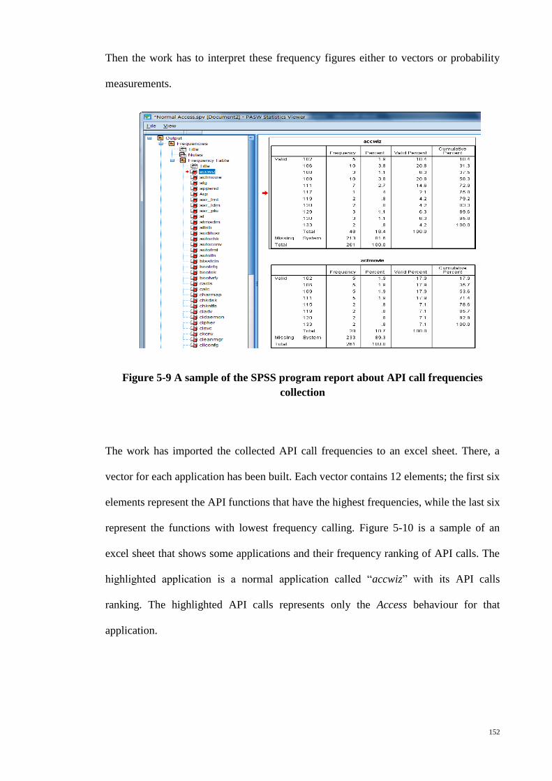
152

Then the work has to interpret these frequency figures either to vectors or probability

measurements.

Figure ‎5-9 A sample of the SPSS program report about API call frequencies

collection

The work has imported the collected API call frequencies to an excel sheet. There, a

vector for each application has been built. Each vector contains 12 elements; the first six

elements represent the API functions that have the highest frequencies, while the last six

represent the functions with lowest frequency calling. Figure 5-10 is a sample of an

excel sheet that shows some applications and their frequency ranking of API calls. The

highlighted application is a normal application called “accwiz” with its API calls

ranking. The highlighted API calls represents only the Access behaviour for that

application.

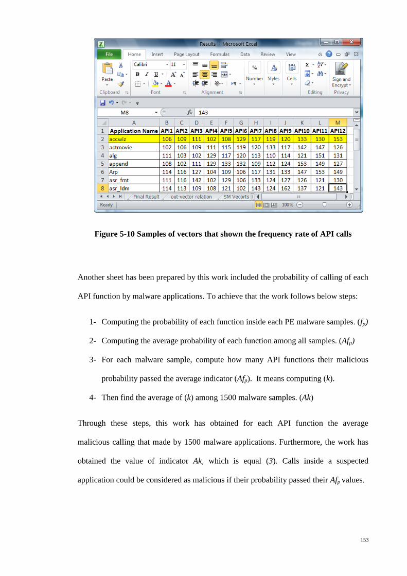
153

Figure ‎5-10 Samples of vectors that shown the frequency rate of API calls

Another sheet has been prepared by this work included the probability of calling of each

API function by malware applications. To achieve that the work follows below steps:

1- Computing the probability of each function inside each PE malware samples. (fp)

2- Computing the average probability of each function among all samples. (Afp)

3- For each malware sample, compute how many API functions their malicious

probability passed the average indicator (Afp). It means computing (k).

4- Then find the average of (k) among 1500 malware samples. (Ak)

Through these steps, this work has obtained for each API function the average

malicious calling that made by 1500 malware applications. Furthermore, the work has

obtained the value of indicator Ak, which is equal (3). Calls inside a suspected

application could be considered as malicious if their probability passed their Afp values.

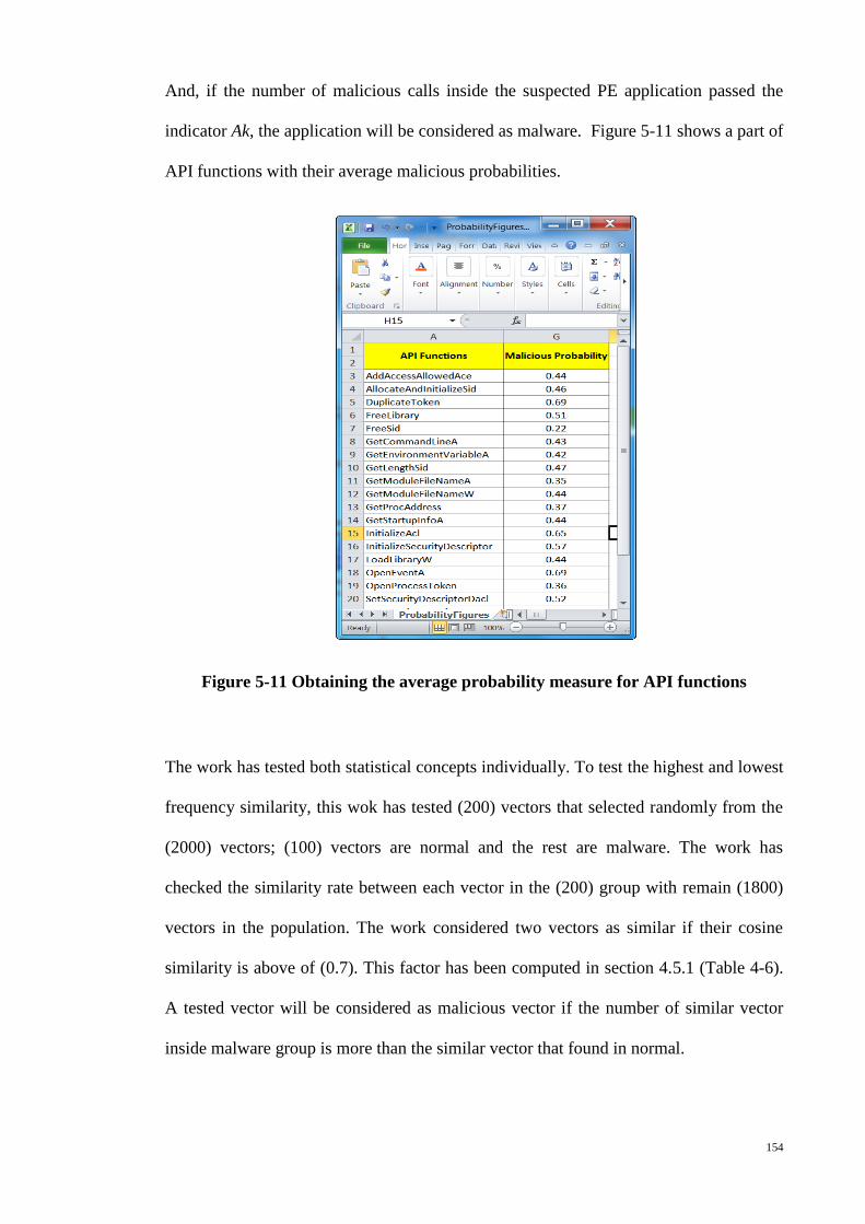
154

And, if the number of malicious calls inside the suspected PE application passed the

indicator Ak, the application will be considered as malware. Figure 5-11 shows a part of

API functions with their average malicious probabilities.

Figure ‎5-11 Obtaining the average probability measure for API functions

The work has tested both statistical concepts individually. To test the highest and lowest

frequency similarity, this wok has tested (200) vectors that selected randomly from the

(2000) vectors; (100) vectors are normal and the rest are malware. The work has

checked the similarity rate between each vector in the (200) group with remain (1800)

vectors in the population. The work considered two vectors as similar if their cosine

similarity is above of (0.7). This factor has been computed in section 4.5.1 (Table 4-6).

A tested vector will be considered as malicious vector if the number of similar vector

inside malware group is more than the similar vector that found in normal.

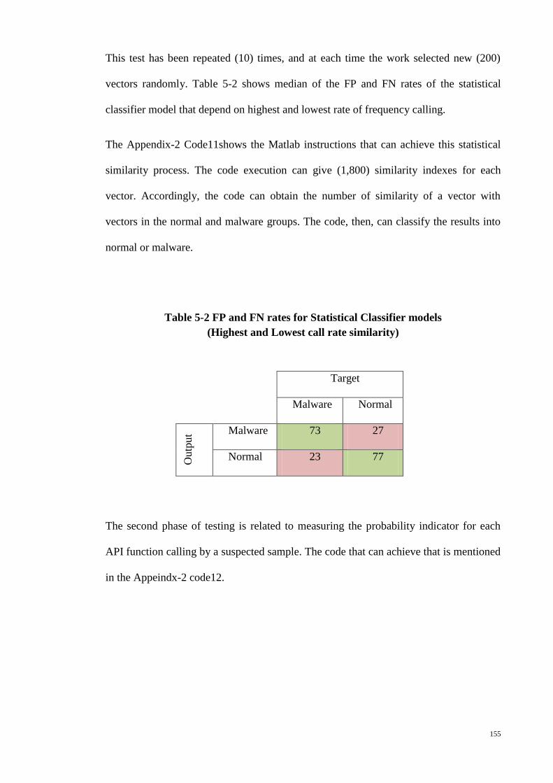
155

This test has been repeated (10) times, and at each time the work selected new (200)

vectors randomly. Table 5-2 shows median of the FP and FN rates of the statistical

classifier model that depend on highest and lowest rate of frequency calling.

The Appendix-2 Code11shows the Matlab instructions that can achieve this statistical

similarity process. The code execution can give (1,800) similarity indexes for each

vector. Accordingly, the code can obtain the number of similarity of a vector with

vectors in the normal and malware groups. The code, then, can classify the results into

normal or malware.

Table ‎5-2 FP and FN rates for Statistical Classifier models

(Highest and Lowest call rate similarity)

Target

Malware Normal

Outp

ut Malware 73 27

Normal 23 77

The second phase of testing is related to measuring the probability indicator for each

API function calling by a suspected sample. The code that can achieve that is mentioned

in the Appeindx-2 code12.

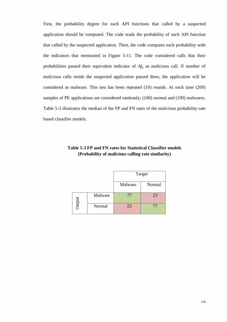
156

First, the probability degree for each API functions that called by a suspected

application should be computed. The code reads the probability of each API function

that called by the suspected application. Then, the code compares each probability with

the indicators that mentioned in Figure 5-11. The code considered calls that their

probabilities passed their equivalent indicator of Afp as malicious call. If number of

malicious calls inside the suspected application passed three, the application will be

considered as malware. This test has been repeated (10) rounds. At each time (200)

samples of PE applications are considered randomly; (100) normal and (100) malwares.

Table 5-3 illustrates the median of the FP and FN rates of the malicious probability rate

based classifier models.

Table ‎5-3 FP and FN rates for Statistical Classifier models

(Probability of malicious calling rate similarity)

Target

Malware Normal

Outp

ut Malware 77 23

Normal 23 77

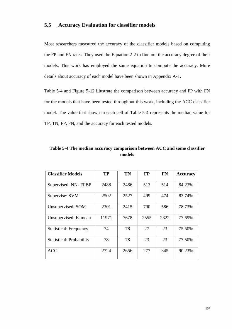
157

5.5 Accuracy Evaluation for classifier models

Most researchers measured the accuracy of the classifier models based on computing

the FP and FN rates. They used the Equation 2-2 to find out the accuracy degree of their

models. This work has employed the same equation to compute the accuracy. More

details about accuracy of each model have been shown in Appendix A-1.

Table 5-4 and Figure 5-12 illustrate the comparison between accuracy and FP with FN

for the models that have been tested throughout this work, including the ACC classifier

model. The value that shown in each cell of Table 5-4 represents the median value for

TP, TN, FP, FN, and the accuracy for each tested models.

Table ‎5-4 The median accuracy comparison between ACC and some classifier

models

Classifier Models TP TN FP FN Accuracy

Supervised: NN- FFBP 2488 2486 513 514 84.23%

Supervise: SVM 2502 2527 499 474 83.74%

Unsupervised: SOM 2301 2415 700 586 78.73%

Unsupervised: K-mean 11971 7678 2555 2322 77.69%

Statistical: Frequency 74 78 27 23 75.50%

Statistical: Probability 78 78 23 23 77.50%

ACC 2724 2656 277 345 90.23%

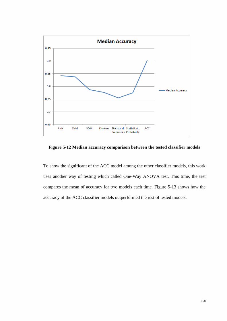
158

Figure ‎5-12 Median accuracy comparison between the tested classifier models

To show the significant of the ACC model among the other classifier models, this work

uses another way of testing which called One-Way ANOVA test. This time, the test

compares the mean of accuracy for two models each time. Figure 5-13 shows how the

accuracy of the ACC classifier models outperformed the rest of tested models.

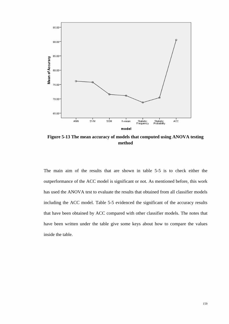
159

Figure ‎5-13 The mean accuracy of models that computed using ANOVA testing

method

The main aim of the results that are shown in table 5-5 is to check either the

outperformance of the ACC model is significant or not. As mentioned before, this work

has used the ANOVA test to evaluate the results that obtained from all classifier models

including the ACC model. Table 5-5 evidenced the significant of the accuracy results

that have been obtained by ACC compared with other classifier models. The notes that

have been written under the table give some keys about how to compare the values

inside the table.

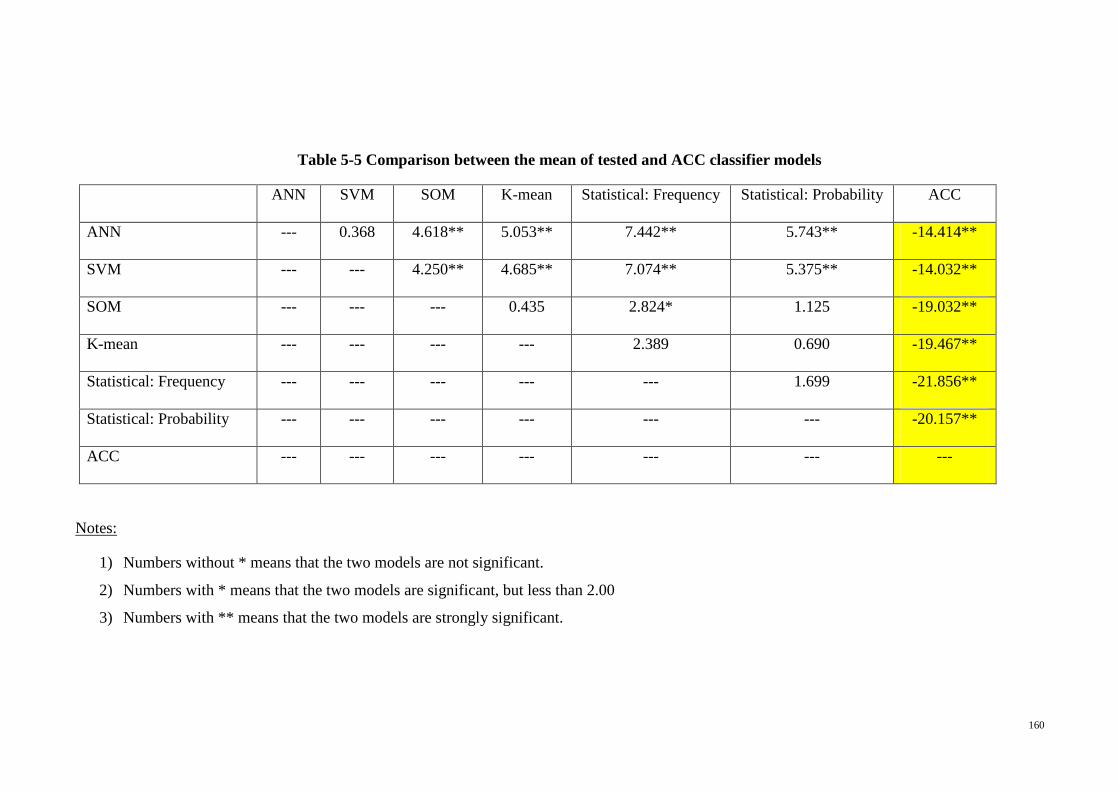
160

Table ‎5-5 Comparison between the mean of tested and ACC classifier models

ANN SVM SOM K-mean Statistical: Frequency Statistical: Probability ACC

ANN --- 0.368 4.618** 5.053** 7.442** 5.743** -14.414**

SVM --- --- 4.250** 4.685** 7.074** 5.375** -14.032**

SOM --- --- --- 0.435 2.824* 1.125 -19.032**

K-mean --- --- --- --- 2.389 0.690 -19.467**

Statistical: Frequency --- --- --- --- --- 1.699 -21.856**

Statistical: Probability --- --- --- --- --- --- -20.157**

ACC --- --- --- --- --- --- ---

Notes:

1) Numbers without * means that the two models are not significant.

2) Numbers with * means that the two models are significant, but less than 2.00

3) Numbers with ** means that the two models are strongly significant.

161

5.6 Chapter Summary

The accuracy of the ACC has been verified with some conversional classifier models.

Through chapter five, this work had shown the process of models verification. Below are

the summery of chapter five:

1- Classifier models could be devised based on different techniques and tools.

2- To test the majority of classifier models with reference to accuracy, this work has

tested the classifier models that more frequently employed by researchers during

the past decade.

3- All used classified models have high rates of False Alarm and Root Mean Square

Errors.

4- The ANOVA test that has been done by this work evidenced that ACC model has

significant outperformance accuracy.

162

Chapter 6

6. Conclusion and Contributions

6.1 Introduction

This chapter is organized in the following manner. The first part presents the conclusions

of the work, with emphasis on the importance of improving the accuracy of classifying

malicious API calls. In addition, this section explains how the direction set by this current

work can support behaviour-based API call detection systems to reveal PE malwares.

The second part of this chapter presents the objectives, all of which were defined and

validated by the work, and describes how each objective was carried out and achieved.

Later, the chapter emphasis the most important contributions of the current work and how

each contribution can positively affect the accuracy of API calling behaviour classifier

systems. The chapter ends by underlining some suggestions for future works.

6.2 Conclusion

Throughout the review stage of this work, we found that most researchers attempted to

classify PE malwares by monitoring the API calls behaviour of malwares. However,

malwares always try to call API functions as normal applications. This behaviour affected

the accuracy of malicious API classifier models, which is problematic. Therefore, this

work addressed the gap of malicious API calls classifier models.

First, the work conducted tests and measured the gaps in the behaviour-based API calls

classifier models. Hence, the work found that the accuracy of API call classifier models

can be improved by controlling errors and by conducting further analysis. The work

searched to find some error controller and confirmation mechanisms. This work found that

163

the functions of a biological phenomenon, called co-stimulation, can be used as a bio-

oriented solution to the problem of gaps in API call classifier models.

Co-stimulation always directs the human immune system to avoid errors. Another function

of co-stimulation is in improving the ability of detectors to use safe and balanced processes

(sections 2.10.1 and 2.10.2). Based on these two processes, this work concluded that

simulating the functionality of co-stimulation as a bio-oriented solution the accuracy of

API calling behaviour classifier models can be improved.

This work has found that the concept of co-stimulation can be attached to most API call

classifier models to increase the certainty of doubtful cases and to improve the

misclassified cases by performing two steps. In the first step, the classifier model can

define the boundaries of these cases that are located in doubtful areas. Second, the model

can clamp them for further investigations and analyses. Through these two steps, the

classifier models, such as ANN, can minimize the FP and FN with RMSE rates

(Table 4-5).

Another interesting discovery is the viewpoint considered by previous researchers in

defining malwares. We found that most researchers defined malwares from the viewpoint

of computer systems or computer users. However, we noted that the viewpoint of detection

and classification systems in defining malwares has not been considered yet. Therefore,

this work concluded a new paradigm for defining malwares based on their behaviours

(6.3.4).

6.3 Achievement of Research Objectives

The objectives are mentioned in Section 1.5. Each objective in this current work is focused

on the process of improving the accuracy of the API call classifier models. Below is the

explanation of each objective in relation to their effect on minimizing errors while

classifying malicious API calls.

164

· Studying different works on malicious API call classifier models

Different perspective and proposals have been made by previous works on malicious

API calling classifier models. Those works had analysed API calling behaviours to

reveal PE malwares through classifying malicious API calls. Reviewing those

projects was the first objective that conducted by this work to collect much

information about this area.

The work initiated this objective to find out the type of models that proposed by

researchers and the tools with methods that utilised by them. The aim of this

objective was also to identify the relation between the behaviours of malwares and

proposed classifier models as well as with the functionalities of the biological viruses

and biological defence systems.

Through achieving this objective the following points become clear:

1- Most works have depended on measuring the similarity between calling

behaviours of unseen malwares with some predefined calling behaviours (Table

2-2 and Table 2-3).

2- Penetrating a normal behaviour for calling API functions by malwares has an

important effect on the accuracy of classifier models as it leads to increase

errors.

3- There is a strong matching between HIS and malware classifier models. This

work obtained through this objective that biological error controller can be

employed to control errors in malicious API classifier models, and then to

improve the accuracy rate.

4- Through this objective, it became clear for this work which type of malwares

should be focused in this research.

165

· For Investigating the functionality and the ability of a biological phenomenon

that can minimize or avoid errors

This work initiated this objective to understand how immune system can control

error when it classify huge amount of biological viruses. Through section (2.10) the

overall work strategy of human immune system has been explained. The section

showed how immune system works and which part of this system can control errors.

The sub-section 2.10.1 has explained the biological error controller that used by the

immune system in more details. Moreover, in sub-section 2.10.2 the concept of

biological error controller, which called co-stimulation, inside the artificial immune

system has been clarified.

In the methodology chapter, especially section 3.5, the designing steps of building a

classifier model including the co-stimulation error controller is clearly explained.

The implementation of the concept of artificial co-stimulation is showed in chapter

four.

Through chapter five and six, the accuracy of Artificial Co-stimulation classifier

model has been discussed and compared with other classifier models (Table 5-4 and

Table 5-6 with Figure 5-12 and Figure 5-13).

· Identifying features that have efficient impact on accuracy of the malicious API

call-classifier models

To validate the accuracy, most classifier models depended on many features. The

most important were the FA and RMSE rates. The FA comes in the four forms,

which are FP, FN, TP, and TN. The value of these four features were substituted in

Equation 2-1 and its result used by most researchers to find the accuracy of their

classifier models. Another form used by researchers to gage the accuracy of classifier

166

models is RMSE, which mentioned in Equation 2-4. Moreover, researchers have

identified different values for the threshold distinguisher that attached to all classifier

models. The main target of this objective was studying the characteristics of these

features.

Targeting this objective helped this work in two ways:

1- As most researches used the FA and RMSE rates for validate the accuracy of

their works with other works, this work should use the same concept to validate

the proposed model, which is ACC, against most important classifier models

that conducted by researchers in Table 2-2 and Table 2-3. Table 5-4 was

resulting from the concept of this objective.

2- Through this objective, the weaknesses of the current threshold value systems

have been revealed. The objective helped this work to find out solutions that

makes threshold value to do other functionalities, such as error controller

(section 4.3.3).

· Building an accurate discrimination model (ACC) and performing validation

Under this section, both objectives that concerned the design and implementation

with validating the ACC model are targeted. The objective has achieved with regard

to FP and FN with RMSE features. The main target of this objective was to design an

accurate malicious API call classifier models, such as ACC, then, to implement and

validate it. These three steps are achieved as indicated below:

1- The parts that mentioned in chapter 3 indicated how to build an accurate model

like ACC.

2- Chapter 4 related to the implementation of ACC.

167

3- Chapter 5 tested the more frequently used classifier model. The result of these

tests was used to validate the ACC accuracy.

6.4 Contribution

The main contribution of our work can be summarised in the following points:

1- Defining a new concept to categorize classifier models.

2- Devising a new bio-oriented malicious API calls classifier model.

3- Identifying new functionality for threshold line distinguisher that attached to

classifier models.

4- New paradigm to define malwares.

Latter parts of this section explain the above-mentioned contributions in detail.

· A new concept to categorise malicious API call-classifier models

Throughout the process of literature review, this current work has found malicious API

classifier models could be categorised into two types of model; biological models and

non-biological models (section 2.9). Although the aim of both types of classier models is

same, their concept and implementation are different.

The concept of biological models depends on some algorithms that occurred inside HIS,

while their implementation depends on a code program that can compute the matching

degree between the shape of detectors and the shape of unknown objects.

On the other side, non-biological models depend on some mathematical and statistical

computation of malwares’ behaviours, where some statistical methods, such as

measuring probability and frequency of API calls, are employed.

168

Categorising classifier models into biological and non-biological may bring attention of

many researchers to do some comparison works between them to propose many types of

accuracy improvement. For instant, researchers can propose some works that can identify

weak points for each type of these models or suggesting ideas of building a hybrid

system between them for better accuracy.

· A new bio-oriented solution for minimizing FP and FN with RMSE errors in

malicious API call-classifier models.

The AIS includes many techniques and algorithms that are employed in different fields

of study. However, most of them are utilized for detection and classification purposes

only (Jieqiong Zheng 2010). Although biologically, the immune system has amazing

interconnected and interrelated procedures and phenomena, only a few bio-oriented

algorithms have been coined independently and employed artificially in AIS (Elgert,

2009; Naik, 2003; Smith, 2006). More research and complementary studies should be

done to improve the ability of these AIS algorithms (U Aickelin et al., 2004; Julie

Greensmith, 2010; Marhusin, Cornforth, et al., 2008; P. T. Zhang et al., 2010; Y Zhang et

al., 2010).

In the field of malware classification, most studies depend on the fundamental algorithm

that was proposed by Forrest et al. (1994; 1997). Based on this algorithm, if a case is not

normal, it can be considered as a malware (Forrest et al., 2002). However, such concept

leads to an increase in the rate of errors, such as false alarms, as every unknown normal

is not always a malware (P. T. Zhang et al., 2010). To avoid such errors, this work found

that IS includes the co-stimulation phenomenon, which undertakes double confirmation

in distinguishing or identifying an unknown cell (Elgert, 2009; Health, 2003). Therefore,

classifier models and detection systems that depend on the algorithm of AIS should also

include this phenomenon in their processes to minimize errors. However, to the best of

169

our knowledge and according to the latest survey on AIS applications (Jieqiong Zheng

2010), the concept of confirmation performed by co-stimulation has not been included in

any research on classification and detection models of malwares .

· New functionalities for the threshold value:

Most of the classifier models and detection systems that proposed previously have

threshold values through which objects can be distinguished. The function ( ) can

represent most, if not all, threshold lines. This function means that all the threshold

values are in a single line, and the only change that occurs from one model to another is

the value of (a).

Models with a single-line threshold value can separate objects into only two classes.

Models that use such discriminator function can position objects in one of its two sides.

On each side of the threshold line, researchers can find a mixture of classified objects

that are high-certainty objects, misclassified objects, and doubtful or low-certainty

objects.

To make the threshold value systems more active in detecting and classifying models,

this study provides a new function for threshold value so that the system can perform

more roles. The new roles that our new threshold value can provide include bonding

most cases that are doubtfully classified and sub-classifying objects into three areas,

namely, pure class one, pure class two, and a class of low-certainty objects. Through

these new functions, the threshold value can support classifier models to identify those

objects that negatively affect the rate of RMSE. This new threshold value can also

identify objects that need more analyses and work to increase their degree of certainty.

Such increase in degree of certainty can reposition some misclassified cases, which in

turn can decrease the FP and FN rates.

170

The support vector machine theory is the only theory that performs its threshold value in

a similar manner to our proposed function. It can collect objects in two classes and then

create a gap between them. However, it cannot activate and utilize this gap to support

more classification models.

· A new paradigm of malwares’‎definition:

Throughout the history of computer viruses and malwares, many definitions of malwares

have been formulated and coined (Bradfield, 2010; Idika & Mathur, 2007). Most of these

definitions describe the activities or the behaviour that malwares perform inside any

infected system. The behaviour described in earlier definitions is analysed and explained

through the lenses of computer systems or computer users. From those definitions,

researchers show ways by which malwares interact with computer systems and reveal the

risks that malwares may bring to users (Szor, 2006).

Some researchers attempted to use another style of defining malwares. They extracted

information from the methodologies of their work and then they used them to define

malwares (M. Alazab et al., 2010; Bayer, Habibi, et al., 2009; Trinius et al., 2011; S. Yu

et al., 2011). However, most of their definitions were still coined within the boundaries

of computer systems and the concepts of computer users.

Our current work initiates a new version of malware definition. We extracted information

from the methodology of the work, but we considered the detection viewpoint of

malwares and classification models. The new version of malware definition states the

following: “Malwares are blocks of codes that are mixed up with normal codes to

perform their payloads smoothly and to defeat detection systems smartly"

The first part of our definition explains the way that malwares can be used to predict

normal applications. This success accurately satisfies the objectives and the methodology

171

of our work. Other definitions always start by describing malwares as unwanted

applications or unprivileged codes that they want to detect.

The second part of our definition shows the behaviour that malwares may perform. The

definition concentrates on two activities: payload execution and defeating techniques.

Although the work payload covers many of the activities of malwares, these are not often

used by researchers to define malwares. However, to date, the concept of the defeating

behaviour of malwares has never been used in any process of defining malwares.

· Supporting other biological models.

Initially, AIS was grounded on simple models of the human immune system. As noted by

Stibor (Xiao & Stibor, 2011), the “first-generation algorithms,” including NSA and CSA,

do not produce the same high quality performance as the human immune system. In

particular, algorithms that conduct negative selections are prone to scaling problems and

generating excessive FA when used to solve problems, such as malware detection

systems. The second-generation algorithm, called Dendretic Cell Algorithm (DCA), was

developed to overcome the problems seen in the NSA. When appropriate threshold

values are used, DCA can generate robust and accurate results in classifying models

(Xiao & Stibor, 2011; Yidan Luo & Jiang, 2008).

Through the proposed model, solutions to the problem of the rate of FA that accompany

NSA and CSA, as well as the problem of identifying an appropriate threshold value

necessary for DCA, are already provided.

172

6.5 Suggested future works

For future works, this work suggests some directions that may make the classification of

malicious API calls more efficient. To achieve that, this work recommended some more

expansion in the parts of the ACC model. Parts that need expansion summarized below:

· Identifying optimum threshold value

Identifying doubtful area for any classifier model may change based on the methods that

used and the dataset that clamped. Through the section 4.4.3, this work could define the

perfect boundaries of active threshold value. It takes many tests to find out these active

values. To make it more efficient, this work suggested an automated step that can give

optimum boundaries for any dataset that may clamped to any classifier model. By this

step, less time required for defining an active threshold value.

This step can support classifier models in another direction. When the boundaries of the

threshold value have been defined, it means defining objects that lie within these

boundaries and need more investigations. Accordingly, the definition of active threshold

can highlight the area where objects doubtfully classified or misclassified.

· More malware policies and behaviours

Since they coded for the first time, malwares have got many modifications and they

behaved differently and more difficultly. They changed from their simplest to more

complicated form. Every span of time, malware analysts recorded new behaviours and

173

activities of malwares. Therefore, to detect malwares based on their behaviours systems

should be up-to-date.

Classifier models usually depend on some training dataset to find out any new cases.

These training sets should cover the valid malware activities and behaviours. Therefore,

this work recommended a process that can identify optimum behaviours from a

malware’s population. Through this identification, classifier models can narrow down to

the necessary behaviours that should be monitored. By this step also, malicious API calls

classifier models can highlight the number and the type of the API functions that should

be covered during training step, and they remained up-to-date with respect to the recent

available malware samples.

174

6.6 Chapter Summary

Contribution and conclusion of this work have been described through the chapter six, and

below are the chapter summary:

1- As far as PE malwares can abuse the API calling behaviour of normal applications,

PE malwares can challenge the malicious API calling classifier models.

2- From the objectives of the researchers;

a. Classifier models are divided into two groups, biological and non-biological

classifier models.

b. Biological co-stimulation is used by human immune system to support

minimizing errors in biological viruses’ classification.

3- It is not necessary for a PE application to call all API functions available inside

computer system. PE applications only need to call the API functions that

necessary for their execution.

4- The long sequence of API functions that called by an application could be broken

down to smaller parts of sequences, which each of them represent a behaviour of

the application during its execution.

175

References

Abdulalla, S. M., Kiah, L. M., & Zakaria, O. (2010). A biological model to improve PE

malware detection: Review. [Acadimic Jounral]. International Journal of the

Physical Sceinces., 5(15), 12.

Ahmadi, M., Sami, A., Rahimi, H., & Yadegari, B. (2011). Iterative System Call Patterns

Blow the Malware Cover. Paper presented at the Security for The Next Generation

2011, KasperSky Lab, TUM, Germany, Garching, Boltzmannstr.

Aickelin, U., Bentley, P., Cayzer, S., Kim, J., & McLeod, J. (2003). Danger theory: The

link between AIS and IDS? Artificial Immune Systems, 147-155.

Aickelin, U., & Cayzer, S. (2002). The danger theory and its application to artificial

immune systems.

Aickelin, U., Greensmith, J., & Twycross, J. (2004). Immune system approaches to

intrusion detection–a review. Artificial Immune Systems, 316-329.

Alanezi, M. M. K., & Aldabagh, N. B. (2012). Using Two Levels dangar model of the

Immune System for Malware Detection. International Journal of Computer Sceince

and Information Security, 10(2), 10.

Alazab, M., Layton, R., Venkataraman, S., & Watters, P. (2010). Malware Detection

Based on Structural and Behavioural Features of API Calls. Paper presented at the

1st International Cyber Resilience Conference, Perth, Western Australia.

Alazab, M., Venkataraman, S., & Watters, P. (2010). Towards Understanding Malware

Behaviour by the Extraction of API Calls. Paper presented at the Cybercrime and

Trustworthy Computing Workshop (CTC), 2010 Second, Ballarat, VIC , Australia.

Alazab, M., Venkatraman, S., & Watters, P. (2011). Zero-day Malware Detection based on

Supervised Learning Algorithms of API call Signatures.

Ali, M. A. M., & Maarof, M. A. (2012). Malware Detection Techniques Using Artificial

Immune System.

Ando, R., Takahashi, K., & Suzaki, K. (2009). A SOM based malware visualization system

using resource access filter of virtual machine.

Antunes, M., & Correia, M. (2011). Tunable immune detectors for behaviour-based

network intrusion detection. Artificial Immune Systems, 6825/2011, 334-347. doi:

10.1007/978-3-642-22371-6_29

Apel, M., Bockermann, C., & Meier, M. (2009). Measuring similarity of malware

behavior.

APIMonitoring.Com. (2010). Win32 API Monitoring Retrieved 15/03/2010, from

http://www.apimonitor.com/index.html

AV-Comparative. (2010, 2010). Report Anti-Virus Comparative February 2010, 2010,

from www.av-comparatives.org/images/stories/test/.../avc_report25.pdf

Bai, L., Pang, J., Zhang, Y., Fu, W., & Zhu, J. (2009). Detecting Malicious Behavior Using

Critical API-Calling Graph Matching. Paper presented at the The 1st International

Conference on Information Science and Engineering (ICISE2009), Nanjing, China.

Basics, D. (2010, Mar 15, 2010 5:18 PM ). An In-Depth Look into the Win32 Portable

Executable File Format - Part 1 Retrieved 20-10-2010, from

http://msdn.microsoft.com/en-us/magazine/bb985992.aspx

http://www.apimonitor.com/index.html

http://www.av-comparatives.org/images/stories/test/.../avc_report25.pdf

http://msdn.microsoft.com/en-us/magazine/bb985992.aspx

176

Bayer, U., Comparetti, P. M., Hlauschek, C., Kruegel, C., & Kirda, E. (2009). Scalable,

behavior-based malware clustering.

Bayer, U., Habibi, I., Balzarotti, D., Kirda, E., & Kruegel, C. (2009). A view on current

malware behaviors.

Bayer, U., Kruegel, C., & Kirda, E. (2006). TTAnalyze: A tool for analyzing malware.

Bergeron, J., Debbabi, M., Desharnais, J., Erhioui, M. M., Lavoie, Y., & Tawbi, N. (2001).

Static detection of malicious code in executable programs. Int. J. of Req. Eng, 184–

189.

Bo-yun Zhang, J.-p. Y., Jin-bo Hao, Ding-xing zhanh and Shu-lin Wang. (2006). Using

Support Vector Machine to Detect Unknown Computer Viruses. International

Journal of Computational Intelligence Research. , 2(1), 100-104.

Boase, J., & Wellman, B. (2001). A Plague of viruses: Biological, computer and

marketing. Current Sociology, 49(6), 39.

Bradfield, S. K. a. J. C. (2010). A General Definition of Malware. [Original Paper].

Journal in Computer Virology, 6(2), 105-114. doi: 10.1007/s11416-009-0137-1

Cha, S.-H. (2007). Comprehensive Survey on Distance/Similarity Measures between

Probability Density Functions. INTERNATIONAL JOURNAL OF

MATHEMATICAL MODELS AND METHODS IN APPLIED SCIENCES, 1(4),

300-307.

Chappell, D. (2006). Understanding .NET: Addison-Wesley Professional.

Cheng Wang, J. P., Rongcai Zhao and Xiaoxian Liu. (2009, 26-29 August, 2009). Using

API Sequence and Byase Algorithm to Detect Suspicious Behavior. Paper presented

at the International Conference on Communications and Networking in China,

Information and Coding Theory Symposium Xi'an, China.

Choi, S., Park, H., Lim, H., & Han, T. (2007). A static birthmark of binary executables

based on API call structure. Advances in Computer Science–ASIAN 2007.

Computer and Network Security, 2-16.

Choi, Y., Kim, I., Oh, J., & Ryou, J. (2009). Encoded Executable File Detection Technique

via Executable File Header Analysis. International Journal of Hybrid Information

Technology, 2(2).

Cohen, F. (1987). Computer viruses:: Theory and experiments. Computers & security,

6(1), 22-35.

Coorp, S. (2008). Symantec Internet Security Threat Report Volume XIII. Whitepaper,

Apr.

D'haeseleer, P. (2002). An immunological approach to change detection: Theoretical

results.

Dabak, P., Phadke, S., & Borate, M. (1999). Undocumented Windows NT: John Wiley

\& Sons, Inc.

Dabek, F., Zhao, B., Druschel, P., Kubiatowicz, J., & Stoica, I. (2003). Towards a common

API for structured peer-to-peer overlays. Peer-to-Peer Systems II, 2735/2003, 33-

44. doi: 10.1007/978-3-540-45172-3_3

Dasgupta, D. (2007). Advances in artificial immune systems. Computational Intelligence

Magazine, IEEE, 1(4), 40-49.

177

Dasgupta, D., Yu, S., & Nino, F. (2010). Recent Advances in Artificial Immune Systems:

Models and Applications. Applied Soft Computing.

Davies, H. (1997). "Signals and Control" Introductory Immunobiology (1 ed., pp. 271-

277).

De Castro, L., & Timmis, J. (2002). Artificial immune systems: a novel approach to pattern

recognition.

de Oliveira, I., Grégio, A., & Cansian, A. (2012). A Malware Detection System Inspired on

the Human Immune System. Computational Science and Its Applications–ICCSA

2012, 286-301.

Ding, J., Jin, J., Bouvry, P., Hu, Y., & Guan, H. (2009). Behavior-Based Proactive

Detection of Unknown Malicious Codes.

Dunham, K. (2011). Malcode Context of API Abuse (pp. 41): SANS Intitute / InfoSec

Reading Room.

Elgert, K. D. (2009). Immunology: understanding the immune system: Wiley-Blackwell.

Essam Al Daoud, I. H. J. a. B. Z. (2008). Computer Virus Strategies and Detection

Methods. International Journal of Open Problems in Computer Science and

Mathematics (IJOPCM), 1(2).

Father, H. (2004). Hooking Windows API - Technics of hooking API functions on

Windows. The CODEBreakers-Journal, 1(2).

Fei Chen, Y. F. (2009). Dynamic Detection of Unknown Malicious Executables Based on

API Interception. Paper presented at the 2009 First International Workshop on

Database Technology and Applications, Chiana.

Focardi, R., Luccio, F., & Steel, G. (2011). An introduction to security API analysis.

Foundations of security analysis and design VI, 35-65.

Forrest, S., Perelson, A., Allen, L., & Cherukuri, R. (2002). Self-nonself discrimination in

a computer. Paper presented at the 1994 IEEE Computer Society Symposium on

Research in Security and Privacy, 1994. Proceedings., Oakland, CA, USA.

Fosnock, C. (2005). Computer Worms: Past, Present, and Future. East Carolina

University.

Fu, W., Pang, J., Zhao, R., Zhang, Y., & Wei, B. (2008). Static Detection of API-Calling

Behavior from Malicious Binary Executables.

Fuyong, Z., & Deyu, Q. (2011). Run-time malware detection based on positive selection.

Journal in Computer Virology, 1-11.

Guerra, L., McGarry, L. M., Robles, V., Bielza, C., Larrañaga, P., & Yuste, R. (2011).

Comparison between supervised and unsupervised classifications of neuronal cell

types: A case study. Developmental neurobiology, 71(1), 71-82.

Hamlen, K. W., Mohan, V., & Wartell, R. (2010). Reining In Windows API Abuses with

In-lined Reference Monitors (Vol. 2010). Dallas, USA: University of Texas

Han, K.-S., Kim, I.-K., & Im, E.-G. (2011). Malware Family Classification Method using

API Sequential Characteristic. (Journal of Security Engineering), 8(2), 4.

Han, K. S., Kim, I. K., & Im, E. G. (2012a). Detection Methods for Malware Variant

Using API Call Related Graphs.

Han, K. S., Kim, I. K., & Im, E. G. (2012b). Malware Classification Methods Using API

Sequence Characteristics.

178

He, Y., Yiwen, L., Tao, L., & Ting, Z. (2010). A model of collaborative artificial immune

system.

Health, N. I. O. (2003). Understanding the Immuney System How it Works. Science

Education.

Heaton, J. (2008). Introduction to Neural Networks for Java: Heaton Research, Inc.

HeavenTools. (2010, 15/03/2010). View, Eidt, and Reverse Engineering EXE and DLL

Files., from http://www.heaventools.com/overview.htm

Hofmeyr, S., & Forrest, S. (1999). Immunity by design: An artificial immune system.

Hofmeyr, S. A., & Forrest, S. (2000). Architecture for an artificial immune system.

Evolutionary Computation, 8(4), 443-473.

Hu, X. (2011). Large-Scale Malware Analysis, Detection, and Signature Generation. The

University of Michigan.

Hu, Y., Chen, L., Xu, M., Zheng, N., & Guo, Y. (2008). Unknown Malicious Executables

Detection Based on Run-Time Behavior.

Huang, H. D., Lee, C. S., Kao, H. Y., Tsai, Y. L., & Chang, J. G. (2011). Malware

behavioral analysis system: TWMAN. Paper presented at the Intelligent Agent (IA),

2011 IEEE Symposium on, Paris, France.

Huang, Y. (2003). Vulnerabilities in Portable Executable (PE) File Format For Win32

Architecture. 19. Retrieved from

http://www.orkspace.net/secdocs/Other/PE/Vulnerabilities%20in%20Portable%20

Executable%20(PE).pdf

HZV. (2010). PE File Structure Retrieved 2010, 2010, from

http://www.thehackademy.net/madchat/vxdevl/papers/winsys/pefile/pefile.htm

Idika, N., & Mathur, A. (2007). A survey of malware detection techniques. Purdue

University.

Islam, M. R., Islam, M. S., & Chowdhury, M. U. (2012). Detecting unknown anomalous

program behavior using API system calls. Informatics engineering and information

science, 383-394.

Ivancevic, V. G. I. a. T. T. (2010). Brain and Classical Neural Network Quantam Neural

Computation (Vol. 40, pp. 43-150). Netherlands: Springer Netherlands.

Iwasaki, A., & Medzhitov, R. (2010). Regulation of adaptive immunity by the innate

immune system. Science, 327(5963), 291.

J-Y. Xu, A. H. S., P. Chavez, S. Mukkamala. (2004, 2004). Polymorphic Malicious

Executable Scanner by API Sequence Analysis. Paper presented at the 4th

International Conference on Hybrid Intelligent Systems (HIS 2004), , Kitakyushu,

Japan.

Jacob, G., Debar, H., & Filiol, E. (2008). Behavioral detection of malware: from a survey

towards an established taxonomy. Journal in Computer Virology, 4(3), 251-266.

Jajodia, S. (2009). Identifying Malicious Code Through Reverse Engineering. In A. Singh

(Ed.), Advances in Information Security (Vol. 44). USA: SpringerLink.

Ji, Z., & Dasgupta, D. (2009). V-detector: An efficient negative selection algorithm with.

Information sciences, 179(10), 1390-1406.

Jiang, H., Mo, W. L., & Qin, J. (2009). An Immune System Algorithm Based on Variable

Detection Radius of the Negative Selection Mechanism.

http://www.heaventools.com/overview.htm

http://www.orkspace.net/secdocs/Other/PE/Vulnerabilities%20in%20Portable%20Executable%20(PE).pdf

http://www.orkspace.net/secdocs/Other/PE/Vulnerabilities%20in%20Portable%20Executable%20(PE).pdf

http://www.thehackademy.net/madchat/vxdevl/papers/winsys/pefile/pefile.htm

179

Jieqiong Zheng , Y. C., and Wei Zhang (2010). A Survey of artificial immune applications

[Journal Article]. Artificial Intelligence Review, 34(2010), 19-34. doi:

10.1007/s10462-010-9159-9

Johanyák, Z. C., & Kovács, S. (2005). Distance based similarity measures of fuzzy sets.

Proceedings of SAMI, 2005.

Julie Greensmith, A. W., and Uwe Aickelin. (2010). Artificial Immune Systems. School of

Computer Science, University of Nottingham: Engineering and Physical Sciences

Research Council (EPSRC). (Reprinted from: 2010).

Khaled, A., Ab d ul-Kader, H., & Ismail, N. (2010). Artificial Immune Clonal Selection

Classification Algorithms for Classifying Malware and Benign Processes Using

API Call Sequences. IJCSNS, 10(4), 31.

Kim, J., & Bentley, P. (2001). An evaluation of negative selection in an artificial immune

system for network intrusion detection.

Kim, J., Greensmith, J., Twycross, J., & Aickelin, U. (2005). Malicious code execution

detection and response immune system inspired by the danger theory.

Kinable, J., & Kostakis, O. (2010). Malware classification based on call graph clustering.

Journal in Computer Virology, 1-13.

Kwon, O., Bae, S., Cho, J., & Moon, J. (2009). Study of fuzzy clustering methods for

malicious codes using native API call frequency.

Lanzi, A., Sharif, M., & Lee, W. (2009). K-Tracer: A system for extracting kernel malware

behavior.

Lee, J., Im, C., & Jeong, H. (2011). A study of malware detection and classification by

comparing extracted strings.

Li, H. J., Tien, C. W., Lin, C. H., Lee, H. M., & Jeng, A. B. (2011, 2011). AOS: An

optimized sandbox method used in behavior-based malware detection. Paper

presented at the Proceedings of the 2011 International Conference on Machine

Learning and Cybernetics, , Guilin - China.

Li, P., Liu, L., Gao, D., & Reiter, M. (2011). On challenges in evaluating malware

clustering.

Li, R. B., Li, A. H., Cai, Y. P., Li, L., & Wang, T. (2010). Euclidean distance based

method for unclassifiable region of support vector machine. Journal of Computer

Applications, 02.

Manzoor, S., Shafiq, M., Tabish, S., & Farooq, M. (2009). A sense of ‘danger’for windows

processes. Artificial Immune Systems, 220-233.

Marhusin, M. F., Cornforth, D., & Larkin, H. (2008, 2008). Malicious Code Detection

Architecture Inspired by Human Immune System. Paper presented at the 2008.

SNPD '08. Ninth ACIS International Conference Software Engineering, Artificial

Intelligence, Networking, and Parallel/Distributed Computing, Phuket.

Marhusin, M. F., Larkin, H., Lokan, C., & Cornforth, D. (2008). An Evaluation of API

Calls Hooking Performance.

McAfee. (2010). McAfee Threats Report: Second Quarter 2010. In n. Q. 2010 (Ed.), (pp.

20).

McGraw, G., & Morrisett, G. (2002). Attacking malicious code: A report to the Infosec

Research Council. Software, IEEE, 17(5), 33-41.

180

Merkel, R., Hoppe, T., Kraetzer, C., & Dittmann, J. (2010). Statistical Detection of

Malicious PE-Executables for Fast Offline Analysis. Communication and

Multimedia Security, 6109/2010, 93-105. doi: 10.1007/978-3-642-13241-4_10

Miao, Q. G., Wang, Y., Cao, Y., Zhang, X. G., & Liu, Z. L. (2010, 2010). APICapture-A

tool for monitoring the behavior of malware. Paper presented at the Advanced

Computer Theory and Engineering (ICACTE), 2010 3rd International Conference,

Chengdu, China.

Miao Wang, C. Z. a. J. Y. (2009). Native API Based Windows Anomaly Intrusion

Detection Methods Using SVM. Paper presented at the International Conference on

Senser Networks, Ubiquitous, and Trustworthy, Taichung, Taiwan.

Michael A. Horan, G. S. A. (1997). Ageing, defence mechanisms and the Immune System.

[Journal Article]. Age and Ageing Oxford Journal, 26-S24: 15-19.

Microsoft. (2008). Microsoft Portable Executable and Common Object File Format

Specification Revision 8.1 – February 15, 2008. . Accessed on 2009, from

http://www.microsoft.com/whdc/system/platform/firmware/PECOFF.mspx

Microsoft. (2011). MSDN Library Retrieved 12/2/2010, 2010, from

http://msdn.microsoft.com/en-us/library/ms123401.aspx

Milenkovi , M., Milenkovi , A., & Jovanov, E. (2005). Using instruction block signatures

to counter code injection attacks. ACM SIGARCH Computer Architecture News,

33(1), 108-117.

Mori, A. (2004). Detecting Unknown Computer Viruses – A New Approach – Lecture

Notes in Computer Science (Vol. 3233/2004, pp. 226-241): Springer Berlin /

Heidelberg.

Nachenberg, C. S. (2001). Northride, CA 91326 (US) Patent No.: I. A. P. U. t. P. C. T.

(PCT).

Naik, S. (2003). Introduction to The Immune System. J Indian Rheumatol Assoc, 11(1,

March 2003), 6.

Nakada, H., Matsuoka, S., Seymour, K., Dongarra, J., Lee, C., & Casanova, H. (2002).

GridRPC: A remote procedure call API for Grid computing. Advanced

Programming Models Research Group, GWD-I (Informational).

Niemela, J., & Palomaki, P. (2011). MALWARE DETECTION BY APPLICATION

MONITORING: WO Patent WO/2011/042,304.

OffensiveComputing. (2010). Offensive Computing Retrieved 11/1/2010, 2010, from


Omer, Y. I. (2009). A WHITELIST BASED IMPLEMENTATION OF ANTIVIRUS-

DEFINITION FILE TO DETECT UNKNOWN MALICIOUS ACTIVITY. Addis

Ababa University.

Oney, W. (2002). Programming the microsoft windows driver model: Microsoft Press

Redmond, WA, USA.

Park, Y., & Reeves, D. (2011). Deriving common malware behavior through graph

clustering.

Parmjit Singh, Chan Yuen Fook, & Sidhu, G. K. (2009). A Comprehensive Guide to

Writing A Research Proposal. Malaysia: Venton Publishing.

http://www.microsoft.com/whdc/system/platform/firmware/PECOFF.mspx

http://msdn.microsoft.com/en-us/library/ms123401.aspx


181

Paul K. Harmer, P. D. W., Gregg H. Gunsch, and Gary B. Lamont. (2002). An Artificial

Immune System Architecture for Computer Security Applications. Paper presented

at the IEEE Transactions on Evolutionary Computation.

Peng, C. F. (2011). Using Aggregation Technology to Improve System Call Based Malware

Behavior Detection. MAster MAster's Thesis.

Pietrek, M. (1994). Peering Inside the PE: A Tour of the Win32 Portable Executable File

Format Retrieved 5/5/2010, 2010

Poggiolini, M. (2008). The Feature Detection Rule and its Application within the Negative

Selection Algorithm. Magister Scientiaw, University of Pretoria, Pretoria, South

Aferica.

Rabek, J. C., Khazan, R. I., Lewandowski, S. M., & Cunningham, R. K. (2003, 2003).

Detection of injected, dynamically generated, and obfuscated malicious code. Paper

presented at the WORM '03 Proceedings of the 2003 ACM workshop on Rapid

malcode New Yourk, NY, USA.

Ramadass, S. (2012). Malware detection based on evolving clustering method for

classification. Scientific Research and Essays, 7(22), 2031-2036.

Rang, H., Dale, M., Ritter, J., & Moore, P. (2003). Pharmacology (Fifth ed.):

CHURCHILL LIVENGSTONE.

Ravi, C., & Manoharan, R. (2012). Malware Detection using Windows API Sequence and

Machine Learning. International Journal of Computer Applications, 43(17), 12-16.

Rieck, K., Holz, T., Willems, C., Düssel, P., & Laskov, P. (2008). Learning and

classification of malware behavior. Detection of Intrusions and Malware, and

Vulnerability Assessment, 108-125.

Rozinov, K. (2005). Efficient static analysis of executables for detecting malicious

behaviors. POLYTECHNIC UNIVERSITY.

Salomon, D. (Ed.). (2010). Elements Of Computer Security. London: SpringerLink.

Sami, A., Yadegari, B., Peiravian, N., Hashemi, S., & Hamze, A. (2010). Malware

detection based on mining API calls.

Schreiber, S. (2001). Undocumented Windows 2000 secrets: a programmer's cookbook:

Addison-Wesley Longman Publishing Co., Inc. Boston, MA, USA.

Schultz, M. G., Eskin, E., Zadok, E., & Stolfo, S. J. (2001). Data mining methods for

detection of new malicious executables. sp, 0038.

Shabtai, A., Moskovitch, R., Elovici, Y., & Glezer, C. (2009). Detection of malicious code

by applying machine learning classifiers on static features: A state-of-the-art

survey. Information Security Technical Report, 14(1), 16-29.

Shafiq, M., Tabish, S., Mirza, F., & Farooq, M. (2009). PE-Miner: Mining Structural

Information to Detect Malicious Executables in Realtime. [Lecture Notes in

Computer Science]. Recent Advances in Intrusion Detection, 5758/2009, 121-141.

doi: 10.1007/978-3-642-04342-0_7

Shankarapani, M., Kancherla, K., Ramammoorthy, S., Movva, R., & Mukkamala, S.

(2010). Kernel machines for malware classification and similarity analysis. Paper

presented at the Neural Networks (IJCNN), The 2010 International Joint

Conference on, Barcelona.

182

Shankarapani, M. K., Ramamoorthy, S., Movva, R. S., & Mukkamala, S. (2011). Malware

detection using assembly and API call sequences. Journal in Computer Virology,

7(2), 107-119.

Shankarpani, M., Kancherla, K., Movva, R., & Mukkamala, S. (2012). Computational

Intelligent Techniques and Similarity Measures for Malware Classification.

Computational Intelligence for Privacy and Security, 215-236.

Shen, H., Wen-Jian, L., & Xu-Fa, W. (2007). A negative selection algorithm with the

variable length detector. Journal of Software, 6.

Sivanandam, S. (2006). Introduction to neural networks using MATLAB 6.0: Tata

McGraw-Hill.

Smith, D. F. a. (Ed.) (2006) (2006 ed., Vols. 6). INDIANA, USA: University of

Evansville.

Solomon, A. (1993). A Brife History of PC Viruses. Computer Fraud and Security

Bulletin, 1993(12), 10.

Spafford, E. H. (1990). Computer Viruses--A Form of Artificial Life?

Srinivasan, S. R. a. S. (2009). Intelligent agent based artificial immune system for

computer security—a review [Journal Article]. Artificial Intelleigence Review,

32(1-4 / December., 2009), 13-43. doi: 10.1007/s10462-009-9131-8

Stibor, T., Mohr, P., Timmis, J., & Eckert, C. (2005). Is negative selection appropriate for

anomaly detection?

Swimmer, M. (2007). Using the danger model of immune systems for distributed defense

in modern data networks. Computer Networks, 51(5), 1315-1333.

Symantec. (2010). Symantec Global Internet Security Threat Report - Trends for 2009

(Vol. XV): Fond in

http://securityresponse.symantec.com/business/theme.jsp?themeid=threatreport.

Szor, P. (1998). Attacks on Win32. Paper presented at the Virus Bulletin Conference,

Munich, Germany.

Szor, P. (2000). Attacks On Win32–Part II. VIRUS, 47.

Szor, P. (2002). USA Patent No.

Szor, P. (2006). The Art of Computer Research and Defence: Addison Wesley Profesional.

Tabish, S. M., Shafiq, M. Z., & Farooq, M. (2009). Malware detection using statistical

analysis of byte-level file content. Paper presented at the CyberSecurity and

Intelligence Informatics New York, NY, USA

Tao, C., Shiguang, J., & Dejiao, N. (2010). NUMERICAL NEGATIVE SELECTION

ALGORITHM. International Journal on Artificial Intelligence Tools, 19(5), 703-

712.

Technology, W. (2010). Virdem Computer Virus, 2010, from

http://virus.wikia.com/wiki/Virdem

Tian, R., Islam, R., Batten, L., & Versteeg, S. (2010). Differentiating malware from

cleanware using behavioural analysis.

Trinius, P., Willems, C., Holz, T., & Rieck, K. (2011). A malware instruction set for

behavior-based analysis.

Vinod, P., Jaipur, R., Laxmi, V., & Gaur, M. (2009). Survey on malware detection

methods.

http://securityresponse.symantec.com/business/theme.jsp?themeid=threatreport

http://virus.wikia.com/wiki/Virdem

183

Vinod, P., Laxmi, V., & Gaur, M. (2011). Scattered Feature Space for Malware Analysis.

Advances in Computing and Communications, 562-571.

VirusSign. (2010). VirusSign Retrieved 11/1/2010, 2010, from


VXHeavens. (2010). VX Heavens Retrieved 11/1/2010, 2010, from

http://vx.netlux.org/vl.php.

Wagener, G., State, R., & Dulaunoy, A. (2008). Malware behaviour analysis. Journal in

Computer Virology, 4(4), 279-287.

Wan, J. (2012). Malware detection using pattern classification: US Patent 8,161,548.

Wang, C., Pang, J., Zhao, R., & Liu, X. (2009). Using api sequence and bayes algorithm to

detect suspicious behavior.

Willems, C., Holz, T., & Freiling, F. (2007). Toward automated dynamic malware analysis

using cwsandbox. IEEE Security & Privacy, 32-39.

Xiang, B., Hao, Y. J., Zhang, Y., & Liu, H. Y. (2008). A novel anti-trojan approach using

behavioral analysis.

Xiangrong Zhang , T. S. a. L. J. (2004). SAR Image Classification Based on Immune

Clonal Feature Selection. SpringerLink, 3212/2004(1611-3349), 504-511. doi:

10.1007/b100438

Xiao, H., & Stibor, T. (2011). A supervised topic transition model for detecting malicious

system call sequences.

Xu, J., Sung, A. H., Mukkamala, S., & Liu, Q. (2007). Obfuscated Malicious Executable

Scanner. Journal of Research and Practice in Information Technology, 39(3), 181-

198.

Yang, T., Deng, H. L., Chen, W., & Wang, Z. (2011). GF-NSA: A Negative Selection

Algorithm Based on Self Grid File. Applied Mechanics and Materials, 44, 3200-

3203.

Ye, Y., Li, T., Jiang, Q., Han, Z., & Wan, L. (2009). Intelligent file scoring system for

malware detection from the gray list.

Ye, Y., Wang, D., Li, T., & Ye, D. (2007). IMDS: Intelligent malware detection system.

Ye, Y., Wang, D., Li, T., Ye, D., & Jiang, Q. (2008). An intelligent PE-malware detection

system based on association mining. Journal in Computer Virology, 4(4), 323-334.

Yegnanarayana1, B. (1994). Artificial neural networks for pattern recognition [Journal

Article ]. Sadhana, 19(2), 189-238. doi: 10.1007/BF02811896

Yidan Luo, & Jiang, Z. (2008, 2008). An Improved Clonal Selection Algorithm and its

Application in Function Optimization Problems. Paper presented at the Second

International Symposium on Intelligent Information Technology Application,

Shangahai, Chian.

Yoshiro Fukushima, Akigiro Sakai, Yoshiaki Hori, & Sakurai, a. K. (2010). A Behavior

Based Malware Detection Scheme to Avoiding False Positive. Paper presented at

the 18th IEEE International Conference on Network Protocols, Kyoto, Japan.

Yu, S., Zhou, S., Liu, L., Yang, R., & Luo, J. (2011). Detecting Malware Variants by Byte

Frequency. Journal of Networks, 6(4), 638-645.

Yu, Y., & Hou, C. (2004). A clonal selection algorithm by using learning operator.


http://vx.netlux.org/vl.php

184

Zakaria, S. M. A. a. O. (2009, 13-19 November, 2009). Devising a Biological Model to

Detect Polymorphic Computer Viruses Artificial Immune System (AIM): Review.

Paper presented at the 2009 International Conference on Computer Technology and

Development, Kota Kinabalu, Malaysia.

Zeng, J., Liu, X., Li, T., Liu, C., Peng, L., & Sun, F. (2009). A self-adaptive negative

selection algorithm used for anomaly detection. Progress in Natural Science, 19(2),

261-266.

Zhang, B., Yin, J., & Hao, J. (2006). Using RS and SVM to Detect New Malicious

Executable Codes. Rough Sets and Knowledge Technology, 574-579.

Zhang, F. Y., Qi, D. Y., & Hu, J. L. (2011a). Run-time malware detection based on IRP.

Journal of South China University of Technology, 39(2), 113-117.

Zhang, F. Y., Qi, D. Y., & Hu, J. L. (2011b). Using IRP for malware detection. Recent

Advances in Intrusion Detection 6307/2010, 514-515. doi:

10.1007/978.3.642.15512.3_39

Zhang, J. J. (2005). Introduction to artificial neural network. Bellingham, WA: Bellingham

AI Robotics Society.

Zhang, P. T., Wang, W., & Tan, Y. (2010). A malware detection model based on a

negative selection algorithm with penalty factor. SCIENCE CHINA Information

Sciences, 53(12), 2461-2471.

Zhang, Y., Li, T., Sun, J., & Qin, R. (2008). A Novel Immune Based Approach for

Detection of Windows PE Virus. Advanced Data Mining and Applications, 250-

259.

Zhang, Y., Pang, J., Yue, F., & Cui, J. (2010). Fuzzy Neural Network for Malware Detect.

Zhang, Y., Song, L. P., & Yang, L. H. (2011). Malicious Codes Detection Inspired by

MHC. Applied Mechanics and Materials, 55, 1642-1647. doi:

10.4028/www.scientific.net/AMM.55-57.1642

Zhang, Y., Wu, L., Xia, F., & Liu, X. (2010). Immunity-Based Model for Malicious Code

Detection. Advanced Intelligent Computing Theories and Applications, 399-406.

Zhao, C. W. J. P. R., & Liu, W. F. X. (2009, 2009). Malware Detection Based on

Suspicious Behavior Identification. Paper presented at the First International

Workshop on Education Technology and Computer Science, 2009. ETCS '09.,

Wuhan, Hubei

Zhao, H., Xu, M., Zheng, N., Yao, J., & Ho, Q. (2010). Malicious executables

classification based on behavioral factor analysis. Paper presented at the 2010.

IC4E '10. International Conference one-Education, e-Business, e-Management, and

e-Learning, Sanya - China.

Zhao, H., Zheng, N., Li, J., Yao, J., & Hou, Q. (2009). Unknown Malware Detection Based

on the Full Virtualization and SVM.

Zhu, L., & Liu, S. (2011, 2011). An experimental comparative study on three classification

algorithms on unknown malicious code identification. Paper presented at the

Multimedia Technology (ICMT), 2011 International Conference, Hanzhou - China.

Zolkipli, M. F., & Jantan, A. (2011, 05 May 2011 ). An approach for malware behavior

identification and classification Paper presented at the 2011 3rd International

Conference on Computer Research and Development (ICCRD), Shanghai - China.

http://www.scientific.net/AMM.55-57.1642

185

Zou, M., Han, L., Liu, Q., & Liu, M. (2009). Behavior-based malicious executables

detection by multi-class SVM. Paper presented at the Information, Computing and

Telecommunication, 2009. YC-ICT '09. IEEE Youth Conference on, Beijing.

Zuben, L. N. C. a. F. J. V. (2001). Learning and Optimization Using Clonal Selection

Principle. IEEE transactions on Evolutionary computation, Special Issue on

Artificial Immune System 2001.

186

Appendix-1

The letter from Peter Szor

Virus Analysis 2 messages

From: WHA080028 student <[email protected]>

<[email protected]> Fri, Mar 19, 2010 at 4:42 PM

To: [email protected]

Dear Sir

I am a PhD student in Network Department - Faculty of Computer Science -University of Malaya. My Name

is “Saman Mirza Abdulla” from Iraq. My research is somehow related to develop a biological model to detect

computer malwares, and now I am in my third semester.

My model has scoped to windows PE file and the function calls that malwares used them during infection

and after. The model currently needed to be analysed with some real malwares to know if the analysed

malwares somehow following the print-foot that drawn by our model or not. For that, we need to trace some

malwares to know how they insert their code inside the PE file and where.

Otherwise, I should trace those malwares, which in that case, needs to download them.

Please, can you advise me how I can get real malware codes or articles that specified virus analysis? In fact, I

found one article in your token about virus analysis in (VB) magazine. In addition to that, your book "Virus

Research and Defence" and some articles published by Symantec became my research backbone.

Your cooperation is highly appreciated.

Thanks in advance for any comments and guides.

Thanks.

Saman Mirza Abdulla --------------------------------------------------------------------------------------------

UNIVERSITY OF MALAYA - " The Leader in Research & Innovation "

mailto:[email protected]

187

Peter Szor [email protected]

To: [email protected] Fri, Mar 19, 2010 at 10:56 PM

Hi Saman,

Thanks for your question. You see, malware samples are never shared outside of the relatively small security

circles, which is really hard to get into. Often, I see this problem at universities, that they would need real

malware. The problem is that by not knowing you, nobody would risk to give samples to you, due to the

impossible justification of its use, and safe handling, without risking the general public. This is true for

trojan, malware, as well as virus samples. In the adware space, there are even more problems, since there is a

lot of copyrighted material in there, and nobody wants to exchange those.

What I would recommend is to either get in touch with another university, or try to find a few sample cases in

virus collections and magazines on the internet. This is not difficult to find.

For your test, if you work with viruses, I would recommend to use something like Funlove to start with. This

small virus is also a network share infector, and it was everywhere at one point of time. This is a simple virus

to profile, based on behaviors.

Then, there are the more difficult types, such as Zmist, which integrates themselves into the executable.

They might not always get call from the file, and they are not at an obvious location either.

Viruses right now are not the greatest issue. Yet, there are cases like polymorphic viruses on the Wildlist.

Reading Virus Bulletin, you can see the names of these threats. The real issue today is malware profiling.

There were over 3 million threats released last year, and most of them are not self replicating threats. They

install themselves often, like real applications, and do their tricks that way.

Depending on which types of threats you need for your test (there are many types in genres) you would need

a honeypot project to capture samples, or have connections to honeypot circles. Real time capturing of

malware, such as worms, bots, trojans is done with virtual machines, or real machines using vulnerable

services connected to the internet. The captures are made on these boxes. This model helps you to get a lot of

malware in a very short time, and allows you to do further research on the classes of interest. This would be

my main recommendation.

There are free honeypot/honeynet projects which you can deploy easily on boxes and collect samples with

them. I wish you good luck collecting the samples, and I apologies, and need your understanding that I

cannot give you live samples of malware code, even for phd research. But having at least 6 million variants

of malware out there, with about 200-300.000 a month, this should not be a problem for you. If nothing, you

could follow the logs of AV at your university to see what comes in, and try to ask your department to save

these samples.

This is how I started.

Best, Peter

mailto:[email protected]

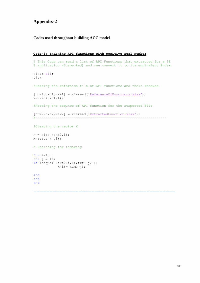
188

Appendix-2

Codes used throughout building ACC model

Code-1; Indexing API functions with positive real number

% This Code can read a list of API Functions that extracted for a PE % application (Suspected) and can convert it to its equivalent index

clear all; clc;

%Reading the reference file of API functions and their Indexes

[num1,txt1,raw1] = xlsread('ReferenceOfFunctions.xlsx'); m=size(txt1,1);

%Reading the sequnce of API function for the suspected file

[num2,txt2,raw2] = xlsread('ExtractedFunction.xlsx'); %=================================================================

%Creating the vector X

n = size (txt2,1); X=zeros (n,1);

% Searching for indexing

for i=1:n for j = 1:m if isequal (txt2(i,1),txt1(j,1)) X(i)= num1(j);

end end end

============================================

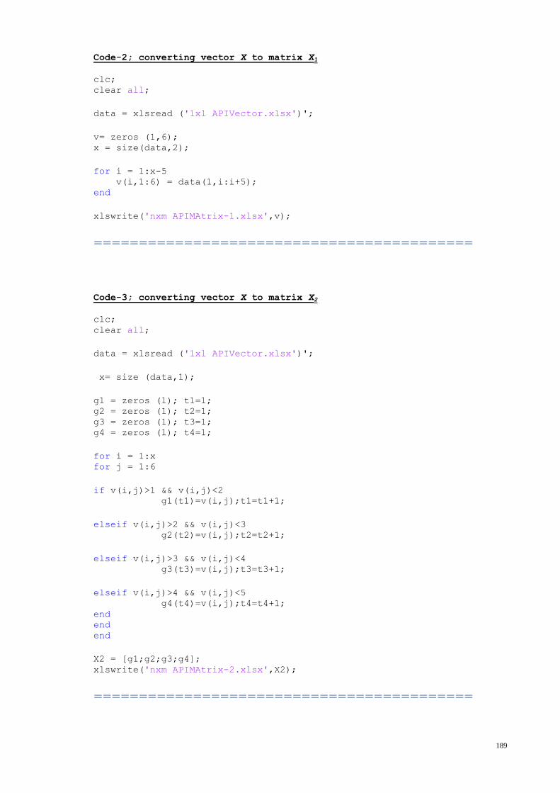
189

Code-2; converting vector X to matrix X1

clc; clear all;

data = xlsread ('1xl APIVector.xlsx')';

v= zeros (1,6); x = size(data,2);

for i = 1:x-5 v(i,1:6) = data(1,i:i+5); end

xlswrite('nxm APIMAtrix-1.xlsx',v);

==========================================

Code-3; converting vector X to matrix X2

clc; clear all;

data = xlsread ('1xl APIVector.xlsx')';

x= size (data,1);

g1 = zeros (1); t1=1; g2 = zeros (1); t2=1; g3 = zeros (1); t3=1; g4 = zeros (1); t4=1;

for i = 1:x for j = 1:6

if v(i,j)>1 && v(i,j)<2 g1(t1)=v(i,j);t1=t1+1;

elseif v(i,j)>2 && v(i,j)<3 g2(t2)=v(i,j);t2=t2+1;

elseif v(i,j)>3 && v(i,j)<4 g3(t3)=v(i,j);t3=t3+1;

elseif v(i,j)>4 && v(i,j)<5 g4(t4)=v(i,j);t4=t4+1; end end end

X2 = [g1;g2;g3;g4]; xlswrite('nxm APIMAtrix-2.xlsx',X2);

==========================================

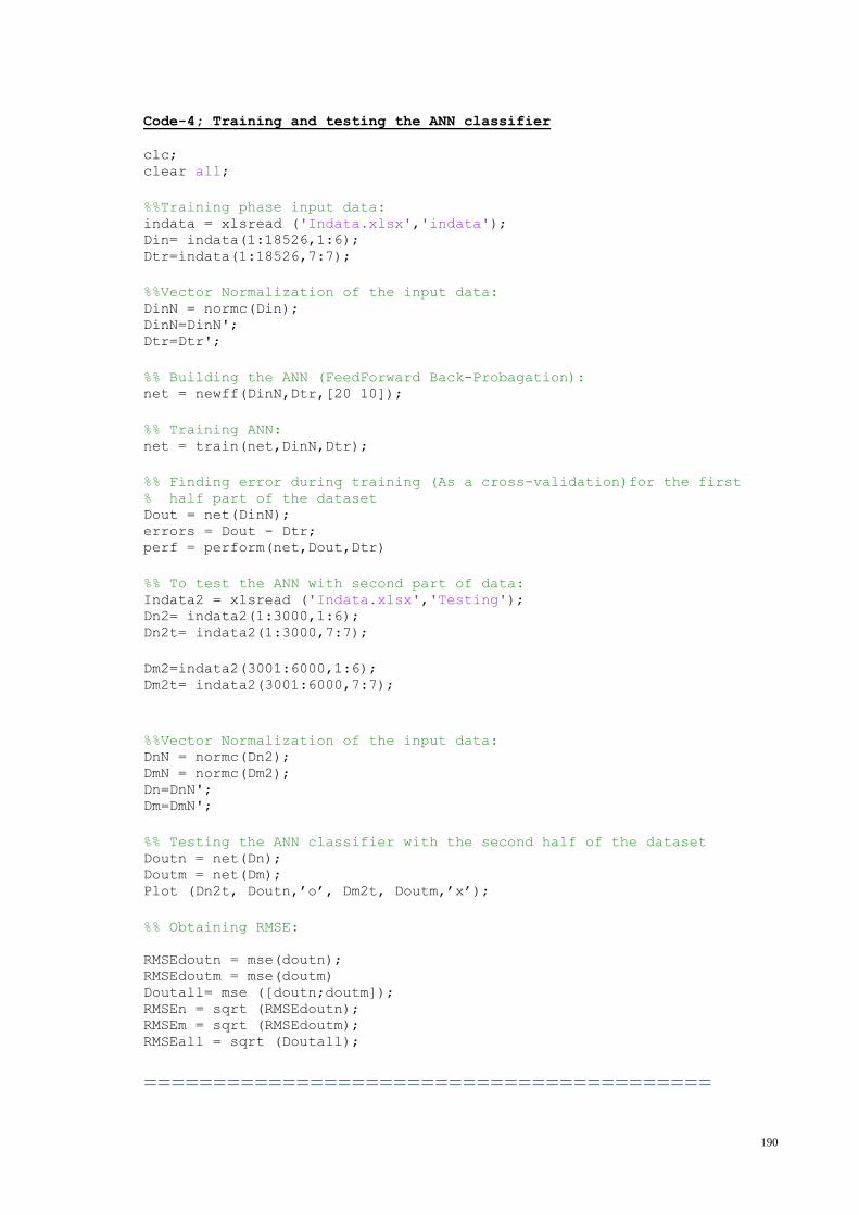
190

Code-4; Training and testing the ANN classifier

clc; clear all;

%%Training phase input data: indata = xlsread ('Indata.xlsx','indata'); Din= indata(1:18526,1:6); Dtr=indata(1:18526,7:7);

%%Vector Normalization of the input data: DinN = normc(Din); DinN=DinN'; Dtr=Dtr';

%% Building the ANN (FeedForward Back-Probagation): net = newff(DinN,Dtr,[20 10]);

%% Training ANN: net = train(net,DinN,Dtr);

%% Finding error during training (As a cross-validation)for the first % half part of the dataset Dout = net(DinN); errors = Dout - Dtr; perf = perform(net,Dout,Dtr)

%% To test the ANN with second part of data:

Indata2 = xlsread ('Indata.xlsx','Testing'); Dn2= indata2(1:3000,1:6);

Dn2t= indata2(1:3000,7:7);

Dm2=indata2(3001:6000,1:6);

Dm2t= indata2(3001:6000,7:7);

%%Vector Normalization of the input data: DnN = normc(Dn2);

DmN = normc(Dm2);

Dn=DnN'; Dm=DmN';

%% Testing the ANN classifier with the second half of the dataset Doutn = net(Dn); Doutm = net(Dm);

Plot (Dn2t, Doutn,’o’, Dm2t, Doutm,’x’);

%% Obtaining RMSE:

RMSEdoutn = mse(doutn);

RMSEdoutm = mse(doutm)

Doutall= mse ([doutn;doutm]);

RMSEn = sqrt (RMSEdoutn);

RMSEm = sqrt (RMSEdoutm);

RMSEall = sqrt (Doutall);

=========================================

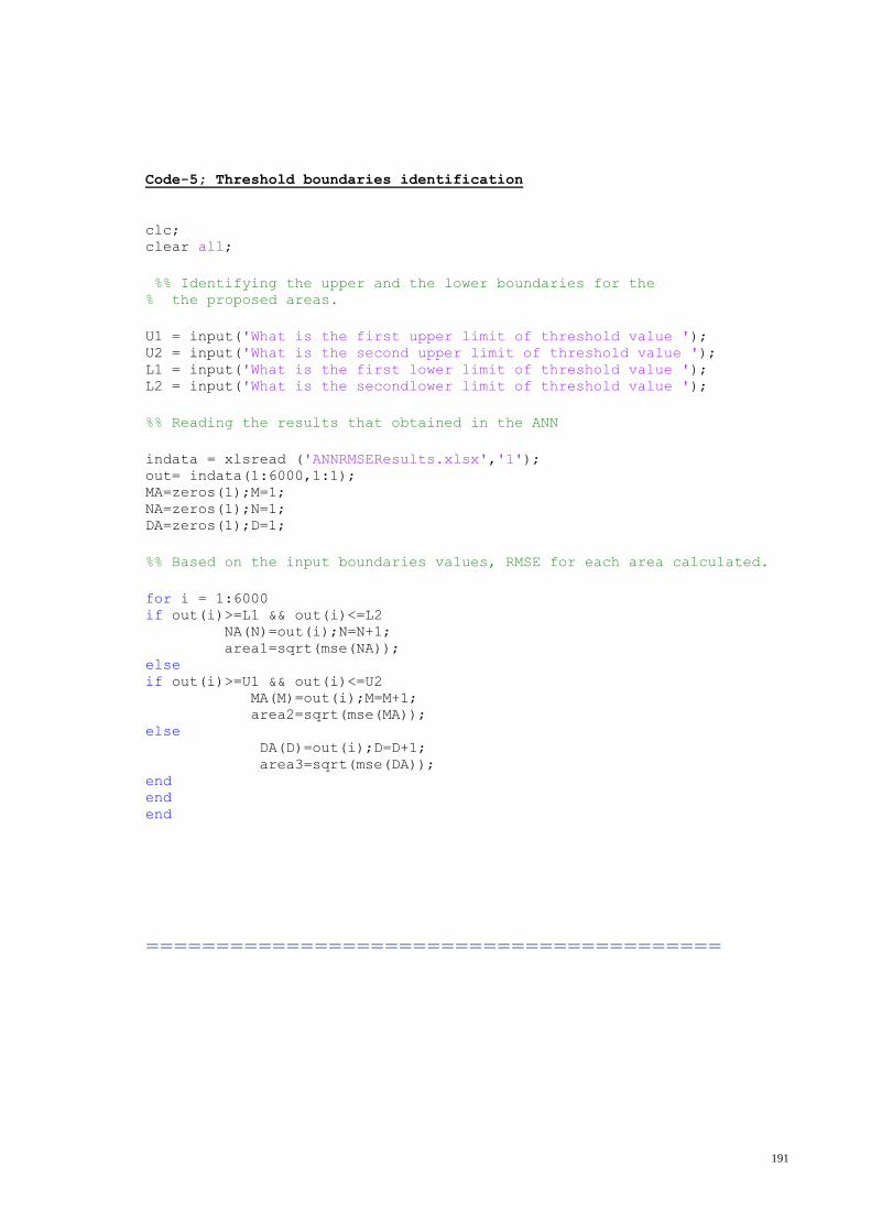
191

Code-5; Threshold boundaries identification

clc; clear all;

%% Identifying the upper and the lower boundaries for the % the proposed areas.

U1 = input('What is the first upper limit of threshold value '); U2 = input('What is the second upper limit of threshold value '); L1 = input('What is the first lower limit of threshold value '); L2 = input('What is the secondlower limit of threshold value ');

%% Reading the results that obtained in the ANN

indata = xlsread ('ANNRMSEResults.xlsx','1'); out= indata(1:6000,1:1); MA=zeros(1);M=1; NA=zeros(1);N=1; DA=zeros(1);D=1;

%% Based on the input boundaries values, RMSE for each area calculated.

for i = 1:6000 if out(i)>=L1 && out(i)<=L2 NA(N)=out(i);N=N+1; area1=sqrt(mse(NA)); else if out(i)>=U1 && out(i)<=U2 MA(M)=out(i);M=M+1; area2=sqrt(mse(MA)); else DA(D)=out(i);D=D+1; area3=sqrt(mse(DA)); end end end

=========================================

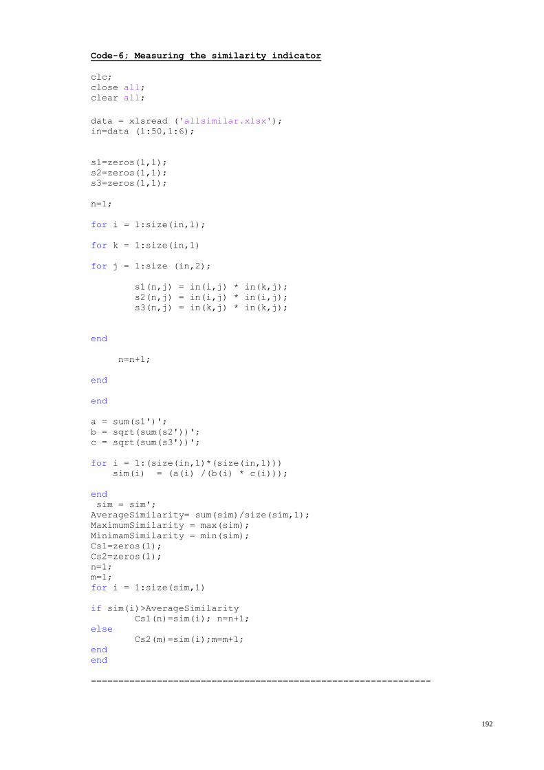
192

Code-6; Measuring the similarity indicator

clc;

close all;

clear all;

data = xlsread ('allsimilar.xlsx');

in=data (1:50,1:6);

s1=zeros(1,1);

s2=zeros(1,1);

s3=zeros(1,1);

n=1;

for i = 1:size(in,1);

for k = 1:size(in,1)

for j = 1:size (in,2);

s1(n,j) = in(i,j) * in(k,j);

s2(n,j) = in(i,j) * in(i,j);

s3(n,j) = in(k,j) * in(k,j);

end

n=n+1;

end

end

a = sum(s1')';

b = sqrt(sum(s2'))';

c = sqrt(sum(s3'))';

for i = 1:(size(in,1)*(size(in,1)))

sim(i) = (a(i) /(b(i) * c(i)));

end

sim = sim';

AverageSimilarity= sum(sim)/size(sim,1);

MaximumSimilarity = max(sim);

MinimamSimilarity = min(sim);

Cs1=zeros(1);

Cs2=zeros(1);

n=1;

m=1;

for i = 1:size(sim,1)

if sim(i)>AverageSimilarity

Cs1(n)=sim(i); n=n+1;

else

Cs2(m)=sim(i);m=m+1;

end

end

==============================================================

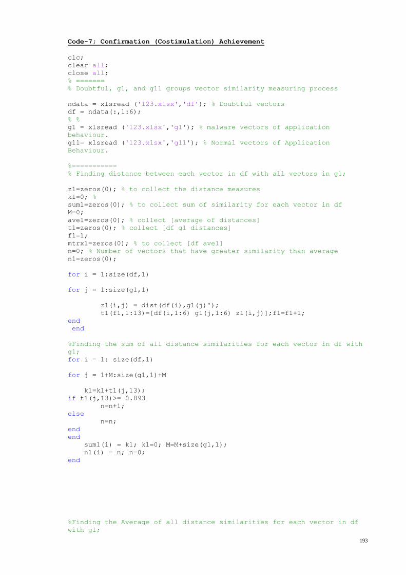
193

Code-7; Confirmation (Costimulation) Achievement

clc;

clear all;

close all;

% =======

% Doubtful, g1, and g11 groups vector similarity measuring process

ndata = xlsread ('123.xlsx','df'); % Doubtful vectors

df = ndata(:,1:6);

% %

g1 = xlsread ('123.xlsx','g1'); % malware vectors of application

behaviour.

g11= xlsread ('123.xlsx','g11'); % Normal vectors of Application

Behaviour.

%===========

% Finding distance between each vector in df with all vectors in g1;

z1=zeros(0); % to collect the distance measures

k1=0; %

sum1=zeros(0); % to collect sum of similarity for each vector in df

M=0;

ave1=zeros(0); % collect [average of distances]

t1=zeros(0); % collect [df g1 distances]

f1=1;

mtrx1=zeros(0); % to collect [df ave1]

n=0; % Number of vectors that have greater similarity than average

n1=zeros(0);

for i = 1:size(df,1)

for j = 1:size(g1,1)

z1(i,j) = dist(df(i),g1(j)');

t1(f1,1:13)=[df(i,1:6) g1(j,1:6) z1(i,j)];f1=f1+1;

end

end

%Finding the sum of all distance similarities for each vector in df with

g1;

for i = 1: size(df,1)

for j = 1+M:size(g1,1)+M

k1=k1+t1(j,13);

if t1(j,13)>= 0.893

n=n+1;

else

n=n;

end

end

sum1(i) = k1; k1=0; M=M+size(g1,1);

n1(i) = n; n=0;

end

%Finding the Average of all distance similarities for each vector in df

with g1;

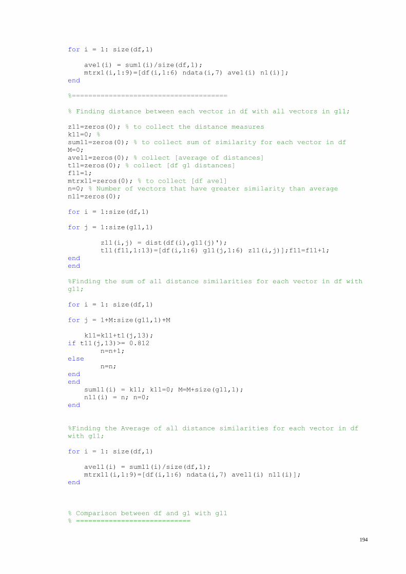
194


ave1(i) = sum1(i)/size(df,1);

mtrx1(i,1:9)=[df(i,1:6) ndata(i,7) ave1(i) n1(i)];

end

%======================================



k11=0; %


M=0;



f11=1;



n11=zeros(0);



z11(i,j) = dist(df(i),g11(j)');

t11(f11,1:13)=[df(i,1:6) g11(j,1:6) z11(i,j)];f11=f11+1;

end

end


g11;



k11=k11+t1(j,13);

if t11(j,13)>= 0.812

n=n+1;

else

n=n;

end

end

sum11(i) = k11; k11=0; M=M+size(g11,1);

n11(i) = n; n=0;

end


with g11;




end

% Comparison between df and g1 with g11

% ============================

195


if (mtrx1(i,8)>=0.893) && (mtrx11(i,8)=<0.812) && (mtrx1(i,9)>=73)...

&& (mtrx11(i,9)=<81)

mtrx1(i,7)=mtrx1(i,7)+mtrx1(i,8)-mtrx11(i,8);

elseif (mtrx11(i,8)>=0.812) && (mtrx1(i,8)=<0.893) &&

(mtrx11(i,9)>=81)...

&& (mtrx1(i,9)=<73)


else

mtrx1 (i,7)=mtrx1(i,7);

end

end

%==================Group g2 and g22 ===========================



k2=0; %


M=0;



f2=1;



n2=zeros(0);




t2(f2,1:13)=[df(i,1:6) g2(j,1:6) z2(i,j)];f2=f2+1;

end

end


g2;



k2=k2+t2(j,13);

if t2(j,13)>= 0.0.914

n=n+1;

else

n=n;

end

end

sum2(i) = k2; k2=0; M=M+size(g2,1);

n2(i) = n; n=0;

end


with g2;



196


end

%======================================



k22=0; %


M=0;



f22=1;



n22=zeros(0);



z22(i,j) = dist(df(i),g22(j)');

t22(f22,1:13)=[df(i,1:6) g22(j,1:6) z22(i,j)];f22=f22+1;

end

end


g22;



k22=k22+t1(j,13);

if t22(j,13)>= 0.835

n=n+1;

else

n=n;

end

end

sum22(i) = k22; k22=0; M=M+size(g22,1);

n22(i) = n; n=0;

end


with g22;




end

%Comparison between df and g2 with g22

% ============================



&& (mtrx22(i,9)=<81)


197


(mtrx22(i,9)>=81)...

&& (mtrx2(i,9)=<73)


else

mtrx2(i,7)=mtrx2(i,7);

end

end

%===================== group g3 and g33 =======================



k3=0; %


M=0;



f3=1;



n3=zeros(0);




t3(f3,1:13)=[df(i,1:6) g3(j,1:6) z3(i,j)];f3=f3+1;

end

end


g3;



k3=k3+t3(j,13);

if t3(j,13)>= 0.876

n=n+1;

else

n=n;

end

end

sum3(i) = k3; k3=0; M=M+size(g3,1);

n3(i) = n; n=0;

end


with g3;




end

%======================================

198



k33=0; %


M=0;



f33=1;



n33=zeros(0);



z33(i,j) = dist(df(i),g33(j)');

t33(f33,1:13)=[df(i,1:6) g33(j,1:6) z33(i,j)];f33=f33+1;

end

end


g33;



k33=k33+t1(j,13);

if t33(j,13)>= 0.817

n=n+1;

else

n=n;

end

end

sum33(i) = k33; k33=0; M=M+size(g33,1);

n33(i) = n; n=0;

end


with g33;




end


% ===========================



&& (mtrx33(i,9)=<59)



(mtrx33(i,9)>=59)...

&& (mtrx3(i,9)=<64)


199

else


end

end

%===================== group g4 and g44 =======================



k4=0; %


M=0;



f4=1;



n4=zeros(0);




t4(f4,1:13)=[df(i,1:6) g4(j,1:6) z4(i,j)];f4=f4+1;

end

end


g4;



k4=k4+t4(j,13);

if t4(j,13)>= 0.883

n=n+1;

else

n=n;

end

end

sum4(i) = k4; k4=0; M=M+size(g4,1);

n4(i) = n; n=0;

end


with g4;




end

%======================================



k44=0; %

200


M=0;



f44=1;



n44=zeros(0);



z44(i,j) = dist(df(i),g44(j)');

t44(f44,1:13)=[df(i,1:6) g44(j,1:6) z44(i,j)];f44=f44+1;

end

end


g44;



k44=k44+t1(j,13);

if t44(j,13)>= 0.827

n=n+1;

else

n=n;

end

end

sum44(i) = k44; k44=0; M=M+size(g44,1);

n44(i) = n; n=0;

end


with g44;




end


% ============================



&& (mtrx44(i,9)=<76)



(mtrx44(i,9)>=76)...

&& (mtrx4(i,9)=<69)


else


end

end

%=======================================================

201

Code-8; Training SVM classifier model to detect malicious API calls

clc;

clear all;

close all;

indata= xlsread ('Indata.xlsx','Normaliz(indata)');

in=indata(1:18526,1:6);

tr=indata(1:18526,7:7);

testin=indata(18527:24526,1:6);

testout=indata(18527:24526,7:7);

svmStruct = svmtrain(in, tr);

classes = svmclassify(svmStruct,testin);

==========================================

202

Code-9; SOM Classifier model

clc; clear all; Close all;

% Solve a Clustering Problem with a Self-Organizing Map % Script generated by NCTOOL % % This script assumes these variables are defined: % % simpleclusterInputs - input data.

num = xlsread ('nxm APIMAtrix-1.xlsx'); num = num (:, 1:6)';

% Create a Self-Organizing Map dimension1 = 2; dimension2 = 2; net = selforgmap([dimension1 dimension2]);

% Train the Network [net,tr] = train(net,num);

% Test the Network d = net(num)';

xlswrite('A.xlsx', d, 1, 'A1');

figure (1),plotsomhits(net,num)

===========================================

203

Code-10; Measuring the accuracy of k-means algorithm to classify API

calls

clc;

clear all;

close all;

indata= xlsread ('k-meandata.xlsx','4');

X=indata(1:2000,1:6);

opts = statset('Display','final');

[idx,ctrs] = kmeans(X,2,...

'Distance','city',...

'Replicates',5,...

'Options',opts);

plot(X(idx==1,1),X(idx==1,2),'b.','MarkerSize',12)

hold on

plot(X(idx==2,1),X(idx==2,2),'r.','MarkerSize',12)

plot(ctrs(:,1),ctrs(:,2),'kx',...

'MarkerSize',12,'LineWidth',2)

plot(ctrs(:,1),ctrs(:,2),'ko',...

'MarkerSize',12,'LineWidth',2)

legend('Normal','Malware','Centroids',...

'Location','NO')

204

Code-11; Similarity measure in statistical based (Frequently) Classifier

model

clc; clear all; close all;

indata = xlsread ('StatVectors.xlsx','StatVector'); m=indata(1:1500,1:12); n=indata(1501:2000,1:12)'; z=zeros(1500,1);x=1;

for i = 1:1500 for j =1501:1550 z(x) = dist(m(i),n(j));x=x+1; end end

g=zeros(1,1500); a=1;b=1500;k=1; c=z(1:750000,1:1);

for j = 1:500

for i = a:b

g(j,k)= z(i,1);k=k+1;

end a=a+1500;b=b+1500;k=1; end

ma=zeros(1);x=1; na=zeros(1);y=1; va=zeros(1);v=1; g2=zeros(1,3);

for i = 401:500 for j = 1:1500 if g(i,j)>=0.7 ma(x)=g(i,j);x=x+1; else if g(i,j)<=0.3 na(y)=g(i,j);y=y+1; else va(v)=g(i,j); end end end

g2(i,1:3)=[size(ma,2),size(na,2),size(va,2)];

end

205

Code-12; Similarity measure in statistical based (Probability) Classifier

model

========================================

% This Code can read a list of API Functions that extracted for a PE % with their probability measure. The Code can compare the probability of % these function with the known malicious probability rate of them % ================================================================ clear all; clc; %% % Reading the reference file of Malicious rate Probability [num1,txt1,raw1] = xlsread('MProbabilityOfFunctions.xlsx'); m=size(txt1,1); %% % Reading the probability rate of each API function that might be called % by the suspected file [num2,txt2,raw2] = xlsread('ProbaOfExtractedFunction.xlsx'); %=================================================================

% Creating the vector X n = size (txt2,1); m = size (txt1,1); X= {n,m}; M=0;

% Searching for indexing

for i=1:n for j = 1:m if isequal (txt2(i,1),txt1(j,1)) && num1(i,1) >=num2(i,1) X{i,1}= (txt2(i,1));X{i,2}=(num2(i,1));M=M+1;

end end end

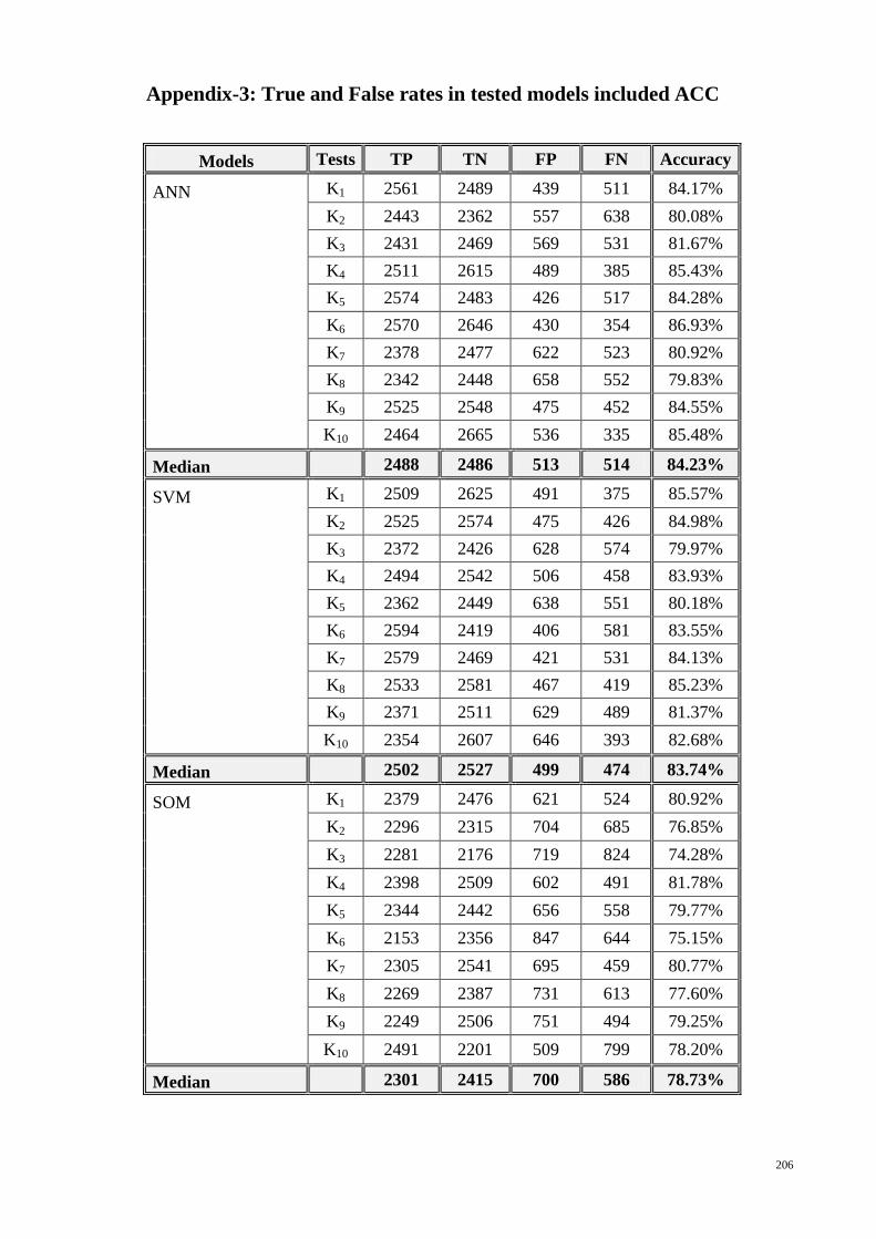
206

Appendix-3: True and False rates in tested models included ACC

Models Tests TP TN FP FN Accuracy

ANN K1 2561 2489 439 511 84.17%

K2 2443 2362 557 638 80.08%

K3 2431 2469 569 531 81.67%

K4 2511 2615 489 385 85.43%

K5 2574 2483 426 517 84.28%

K6 2570 2646 430 354 86.93%

K7 2378 2477 622 523 80.92%

K8 2342 2448 658 552 79.83%

K9 2525 2548 475 452 84.55%

K10 2464 2665 536 335 85.48%

Median 2488 2486 513 514 84.23%

SVM K1 2509 2625 491 375 85.57%

K2 2525 2574 475 426 84.98%

K3 2372 2426 628 574 79.97%

K4 2494 2542 506 458 83.93%

K5 2362 2449 638 551 80.18%

K6 2594 2419 406 581 83.55%

K7 2579 2469 421 531 84.13%

K8 2533 2581 467 419 85.23%

K9 2371 2511 629 489 81.37%

K10 2354 2607 646 393 82.68%

Median 2502 2527 499 474 83.74%

SOM K1 2379 2476 621 524 80.92%

K2 2296 2315 704 685 76.85%

K3 2281 2176 719 824 74.28%

K4 2398 2509 602 491 81.78%

K5 2344 2442 656 558 79.77%

K6 2153 2356 847 644 75.15%

K7 2305 2541 695 459 80.77%

K8 2269 2387 731 613 77.60%

K9 2249 2506 751 494 79.25%

K10 2491 2201 509 799 78.20%

Median 2301 2415 700 586 78.73%

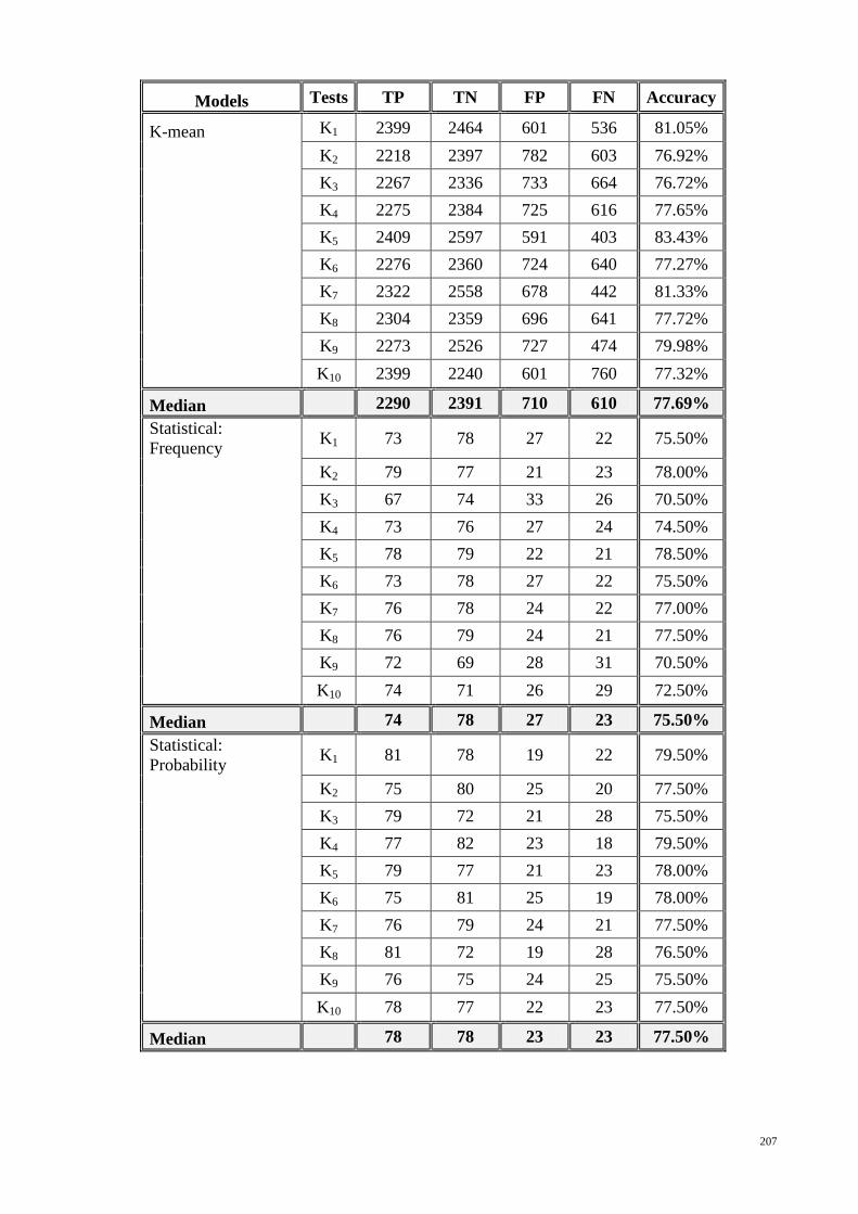
207


K-mean K1 2399 2464 601 536 81.05%

K2 2218 2397 782 603 76.92%

K3 2267 2336 733 664 76.72%

K4 2275 2384 725 616 77.65%

K5 2409 2597 591 403 83.43%

K6 2276 2360 724 640 77.27%

K7 2322 2558 678 442 81.33%

K8 2304 2359 696 641 77.72%

K9 2273 2526 727 474 79.98%

K10 2399 2240 601 760 77.32%

Median 2290 2391 710 610 77.69%

Statistical:

Frequency K1 73 78 27 22 75.50%

K2 79 77 21 23 78.00%

K3 67 74 33 26 70.50%

K4 73 76 27 24 74.50%

K5 78 79 22 21 78.50%

K6 73 78 27 22 75.50%

K7 76 78 24 22 77.00%

K8 76 79 24 21 77.50%

K9 72 69 28 31 70.50%

K10 74 71 26 29 72.50%

Median 74 78 27 23 75.50%

Statistical:

Probability K1 81 78 19 22 79.50%

K2 75 80 25 20 77.50%

K3 79 72 21 28 75.50%

K4 77 82 23 18 79.50%

K5 79 77 21 23 78.00%

K6 75 81 25 19 78.00%

K7 76 79 24 21 77.50%

K8 81 72 19 28 76.50%

K9 76 75 24 25 75.50%

K10 78 77 22 23 77.50%

Median 78 78 23 23 77.50%

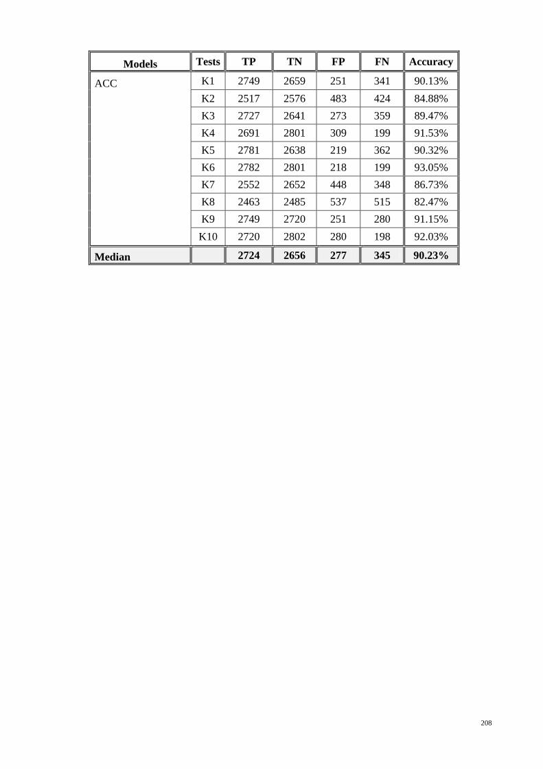
208


ACC K1 2749 2659 251 341 90.13%

K2 2517 2576 483 424 84.88%

K3 2727 2641 273 359 89.47%

K4 2691 2801 309 199 91.53%

K5 2781 2638 219 362 90.32%

K6 2782 2801 218 199 93.05%

K7 2552 2652 448 348 86.73%

K8 2463 2485 537 515 82.47%

K9 2749 2720 251 280 91.15%

K10 2720 2802 280 198 92.03%

Median 2724 2656 277 345 90.23%

Documents

an artificial co-stimulation classifier for malicious api - UM