As

RSa

5b

c

a

ARRA

KIQER

1

sdavt2

s(s(wiaui

a

h0

Agricultural and Forest Meteorology 195–196 (2014) 179–191

Contents lists available at ScienceDirect

Agricultural and Forest Meteorology

j our na l ho me page: www.elsev ier .com/ locate /agr formet

mmonia volatilisation following urea fertilisation in an irrigatedorghum crop in Italy

.M. Ferraraa, B. Loubetb,∗, C. Decuqb, A.D. Palumboa, P. Di Tommasic, V. Magliuloc,. Massonb, E. Personneb, P. Cellierb, G. Ranaa

Consiglio per la Ricerca e la sperimentazione in Agricoltura – Research Unit for cropping systems in dry environments (CRA – SCA), Via Celso Ulpiani, – 70125 Bari, ItalyINRA, UMR INRA-AgroParisTech, 1091 Environnement et Grandes Cultures, 78850 Thiverval-Grignon, FranceCNR – ISAFoM, Via Patacca 85, Ercolano (Na), Italy

r t i c l e i n f o

rticle history:eceived 15 November 2013eceived in revised form 30 April 2014ccepted 20 May 2014

a b s t r a c t

Ammonia (NH3) fluxes were estimated by three inverse modelling methods over a sorghum field fol-lowing the application of 240 kg N ha−1 of urea pills under a semi-arid Mediterranean climate. Ammoniavolatilisation started following irrigation, which coincided with the third urea application. The maximumvolatilisation rate was reached 7 days after irrigation. A clear dependence of the NH3 volatilisation on

−2 −1

eywords:nverse modellingC-TILDASmission factoresistance model

irrigation and rainfall events was observed. The NH3 fluxes ranged from −2.5 to 45 �g NH3 m s . Thecanopy compensation point jumped from 9 �g NH3 m−3 before urea hydrolysis to 131 �g NH3 m−3 after-wards, while the soil compensation point varied in the meantime from 24 to 800 �g NH3 m−3 on average.The soil-dominated observed NH3 emissions were reasonably well reproduced by a two-layer resistancemodel. Overall, between 10% and 14% of the total nitrogen applied was volatilised.

© 2014 Elsevier B.V. All rights reserved.

. Introduction

The nitrogen (N) cycle is greatly affected by human activitiesuch as fertilizer production (Haber-Bosch process), energy pro-uction, combustion and changes in land use, generating increasedmounts of reactive N (Nr) in the environment which leads toarious threats to aquatic and terrestrial ecosystems, as well aso human health through atmospheric pollution (Galloway et al.,008), while being beneficial for crop and food production.

Agriculture is responsible for over 90% of ammonia (NH3) emis-ions in Europe (EMEP/EEA and guidebook, 2013) and 95% in ItalyRomano et al., 2013). In particular, field applied manure is the mainource of atmospheric NH3, followed by mineral N fertilizer useECETOC, 1994). Among these, urea accounts for 50% of the totalorld fertilizer consumption and is steadily increasing in develop-

ng countries. In Italy, about 40% of N is applied as urea, although trend in application reduction has been recorded. Field-appliedrea contributes to about 4% of the anthropogenic NH3 emissions

n Western Europe (ECETOC, 1994).The amount of NH3 volatilised is a variable percentage of the

pplied NH3, depending on several factors such as the fertilizer

∗ Corresponding author. Tel.: +33 (0)1 30 81 55 33.E-mail address: loubet@grignon.inra.fr (B. Loubet).

ttp://dx.doi.org/10.1016/j.agrformet.2014.05.010168-1923/© 2014 Elsevier B.V. All rights reserved.

type, the application technique, the soil type and humidity, theweather conditions and the crop cover (e.g. Sommer et al., 2003).NH3 volatilisation increases with soil ammonium (NH4

+) content,soil pH and soil temperature, while soil microbial population andorganic matter content impacts the amount of NH4

+ (van derWeerden and Jarvis, 1997).

While several studies on NH3 volatilisation after slurry/manurespreading can be found for different environments (e.g. Carozziet al., 2013a, 2013c; Huijsmans et al., 2003; Monteny and Erisman,1998; Pain et al., 1998; Sintermann et al., 2012; Sommer andHutchings, 2001), few data are available for NH3 losses by ureaunder semi-arid conditions (Das et al., 2008) while these conditionswould characterise approximately 12% of European and MiddleEastern land (Gao and Giorgi, 2008). Consequently, inappropriateNH3 emission factors may be used for urea in these semi-arid condi-tions (20% of the N applied is used in the EMEP/EEA and guidebook,2013). Among the few data available by micrometeorological meth-ods in semi-arid conditions, Sanz-Cobena et al. (2008) and Pacholskiet al. (2006) reported NH3 losses of about 10% and 48% of the urea-N applied, using the integrated horizontal flux method, a methodwhich may overestimate NH3 emissions (Sintermann et al., 2012).

Additionally, Roelcke et al. (1996) reported NH3 losses of about 60%of surface applied urea in 13 days under semi-arid conditions, whileZhang et al. (1992) found that between 30% and 32% of the N appliedas urea could be lost as NH3 from calcareous soils in North China.

1 rest M

Ftl

ecLdssLtbmcy

fC2WQd

aSSemice

flmdapf

2

2

2Islap7Mwp

vhdow1cb

80 R.M. Ferrara et al. / Agricultural and Fo

urthermore, understanding NH3 volatilisation dynamics is criticalo identifying best management practices and to extrapolating NH3osses over larger scales.

Measuring NH3 fluxes is nevertheless still difficult. Acknowl-dged methods include the aerodynamic gradient (AG), the eddyovariance (EC), and the inverse modelling (IM) methods (see e.g.,oubet et al., 2010). The aerodynamic gradient method with wetenuders and conductivity analysis with gaseous separation on aemi-permeable membrane is still the reference method for mea-uring NH3 fluxes (Flechard and Fowler, 1998; Flechard et al., 2010;oubet et al., 2012; Sutton et al., 1993, 2008). Recently, the condi-ional time averaged gradient (COTAG) method has been developedased on time integration of the AG method conditioned by ther-al stability (Famulari et al., 2009), to allow longer term and low

ost monitoring of NH3 fluxes, but these may not be well adaptedet for very unstable conditions.

The eddy covariance (EC) technique has been recently availableor NH3 with the development of highly sensitive and fast Quantumascade Laser (QCL) devices (Brodeur et al., 2009; Famulari et al.,004; Ferrara et al., 2012; Shaw et al., 1998; Sintermann et al., 2011;hitehead et al., 2008). But NH3 flux measurement by EC with a

CL could be difficult due to the interaction of NH3 with water andust in the tubes.

Inverse dispersion methods are also increasingly used to evalu-te NH3 losses following slurry application using either Lagrangiantochastic models (Flesch et al., 2007; McGinn et al., 2007;intermann et al., 2012; Sommer et al., 2005) or Gaussian mod-ls (Loubet et al., 2001, 2010) or both (Carozzi et al., 2013c). Theseethods are very well adapted for geometrically well-defined and

solated sources, and have been demonstrated as being valid whenompared to reference methods in the case of high fluxes (Loubett al., 2010; Sintermann et al., 2012).

In this study, we analyse ammonia fluxes above a sorghum crop,ollowing application of urea pills, in the semi-arid region of Apu-ia (Italy). The fluxes were estimated with three inverse modelling

ethods. A resistance model is used to interpret the NH3 fluxynamics and identify its soil and plant components. The canopynd soil compensation points are evaluated and compared to soilH and NH4

+ measurements and discussed. Finally the emissionactor of NH3 volatilisation following urea application is estimated.

. Materials and methods

.1. Field site and nitrogen application

The experimental campaign was carried out from 17 to 30 July008 in Rutigliano (41′N, 17◦54′ E, 122 m a.s.l.) near Bari in Southerntaly in a 2 ha flat field of growing Sorghum vulgare (cv Hay Day)owed on 10 June 2008 and irrigated with a sprinkler. The soil is aoamy clay (Clay 41%; Silt 44%; Sand 15%), with a porosity of 52%,

bulk density of 1.15 kg L−1, a field capacity of 29% and a wiltingoint of 17%. The pH(H2O) was 7.8, while the pH(KCl) was around.0 during the experimental campaign. The climate is semi-aridediterranean, with hot and dry summers and short and temperateinters with mean annual temperature of 15.7 ◦C and mean annualrecipitation of 600 mm.

The crop was very heterogeneous with a mean leaf area indexarying from 1.0 to 5.0 m2 m−2 (Licor 3100, USA) and an averageeight from 0.72 to 1.25 m. Single sided LAI and plant height wasetermined 2 times per week on 10 plants. In total 240 kg N ha−1

f urea (46% N content commercial name; Fertilsud s.r.l., Italy)

as applied in granular form in three applications: 30, 90 and

20 kg N ha−1 on 1, 16 and 22 July 2008. The first and second appli-ations were done under dry conditions (applying 7.9 mm of watery irrigation only before urea spreading), while 9.3 mm of water

eteorology 195–196 (2014) 179–191

was applied before and after the third application. The amountof urea applied was slightly larger than usual agronomic practicesfor irrigated sorghum (150–200 kg N ha−1; Giardini and Vecchietti,2000).

2.2. Site experimental monitoring

A summary of the variables monitored is given in Table 1.The meteorological data (air temperature, relative humidity, globalradiation, reference evapotranspiration, wind speed, wind direc-tion and rainfall) were measured with a standard meteorologicalstation placed on a reference grass field located near the exper-imental field with all sensors at 2 m above ground. The othermeteorological data (net radiation, incoming and outgoing globalradiation, infrared surface temperature, wind speed and direction,air temperature and relative humidity) were measured in the mid-dle of the experimental field every 10 s and averaged over one hourtime intervals with a data logger (CR10X, Campbell Sci., Shepshed,UK). Soil samples were also collected every three to four days, atrandom locations at 0–0.2 and 0.2–0.4 m depths for the volumetricsoil water content and at 0.2–0.4 m depth for soil available nitrate(NO3

−), NH4+ and pH.

2.3. Heat, water vapour and CO2 fluxes by eddy covariance

Heat, water vapour and carbon dioxide (CO2) fluxes were mea-sured by eddy covariance, with a tri-axial ultrasonic anemometer(Gill R2, Gill Instruments Ltd, UK), and a H2O/CO2 open path infraredabsorption analyser (Li-Cor 7500, USA) located near the centre ofthe field at zm = 1.3 m and zm = 1.6 m height (changed on the 26July). The fetch was around 120 m in the prevalent wind direction,which is a short fetch for EC measurements. The flux footprint wasestimated with the Kormann and Meixner (2001) model using aroughness length z0 of 0.06 m. The percentage of flux footprint inthe field was found to range from 68% to 96% (for u* > 0.1 m s−1) andaveraged 84%. The wind sector 240–300 deg/N was the most criti-cal sector with only 72% of the flux footprint in the field. The eddycovariance fluxes of CO2, latent (LE) and sensible heat (H), as wellas the friction velocity (u*) and the Obukhov length (L) were calcu-lated as in Aubinet et al. (2000). The Eddysoft package (Kolle andRebmann, 2007) was used to acquire and to calculate half-hourlymean eddy fluxes.

2.4. NH3 concentrations with a QC-TILDAS

NH3 concentration was measured with the compact QC-TILDAS-76 (SN002-U, Aerodyne Research Inc., ARI, USA; Zahniser et al.,2005). An accurate description of the device can be found inMcManus et al. (2008) and Nelson et al. (2004), while Ellis et al.(2010) evaluated the performance of the instrument. In this trial, a2.5 m long 0.75 cm inner diameter PFA tube was used as the inlet forthe QC-TILDAS. The NH3 concentrations of the QCL were calibratedto match the concentrations of the diffusion samplers, described inthe following, with a calibration factor of 2.86 ± 0.09 as discussedin Ferrara et al. (2012).

2.5. Estimation of NH3 fluxes by inverse modelling

NH3 flux was estimated by inverse modelling using the concen-tration measured at the EC mast by the QCL (C(zm)) and backgroundNH3 concentration (Cbgd) was estimated as the minimum of threesets of diffusion samplers (Tang et al., 2001) located at 100 m, 100 m

and 300 m on the north, south and west of the field (Fig. 1) andchanged weekly. The inverse modelling methods have been exten-sively detailed in Flesch et al. (1995, 2004, 2005a, 2005b, 2007)and the methodology used here detailed in Loubet et al. (2010)

R.M. Ferrara et al. / Agricultural and Forest Meteorology 195–196 (2014) 179–191 181

Table 1Details of the measurements setup.

Measurement Symbol Unit Details

Meteorology (inthe field)

Wind speed U m s−1 Cup anemometer (A100, Vector Inst., USA) at 2 mWind direction WD deg/N Potentiometer wind vane W200P (Campbell Sci.,

Shepshed, UK) at 5 mAir temperature Ta

◦C Thermo-hygrometer (M100, Rotronic, USA) at 2 mRelative humidity RH % Thermo-hygrometer (M100, Rotronic, USA) at 2 mGlobal radiation Rg W m−2 Albedometer (Li-200, LI-COR, USA) for incoming and

out coming global radiation at 2 mPrecipitation P mm Tipping bucket rain gauge (ARG100, Campbell Sci.,

Shepshed, UK).

Diffusion samplers Background concentration Cbgd �g NH3 m−3 ALPHA samplers located at 100 m, 100 m and 300 m onthe north, south and west of the field

Concentration with QCL-TILDAS NH3 concentration C(zm) �g NH3 m−3 NH3 fast analyser (QC-TILDAS-76 SN002-U, AerodyneResearch Inc., USA)

Soil and cropsurface

Soil water content at 0–0.2 and0.2–0.4 m depths

WC kg kg−1 Gravimetric measurements

Soil temperature at 0.1 and0.3 m, depths,

Ts◦C Thermistors (107, Campbell Sci., Shepshed, UK). Depths

N-NO3− and N-NH4

+

concentrations at 0.2–0.4 mdepth

[NO3−] [NH4

+] mg kg−1 dry soil Molecular absorption spectroscopy (colorimetricreactions: of Griess-Ilosvay for NO3

− and of Berthelotfor NH4

+) (Model AutoAnalyzer II, Bran Luebbe,

aianaF

F

Fptt1

pH at 0.2 – 0.4 m depth pH

Infrared Surface Temperature Tz0′

nd Carozzi et al. (2013c). Briefly, the field is considered as hav-ng a homogeneous flux FNH3(zm). The half-hourly concentrationt the EC mast location, Cmodel, is modelled using u*, L, the rough-ess length (z0) and the wind direction (WD) from the ultrasonicnemometer with a modelled flux Fmodel = 1 ng NH3 m−2 s−1. FinallyNH3(zm) is evaluated as:

NH3 (zm) = C(zm) − Cbgd

Cmodel× Fmodel (1)

ig. 1. Map of the field site. The green rectangle is the sorghum crop, the blueoint is the eddy covariance mast and met station location, the yellow square ishe additional met station location and the red stars are the background concen-ration sampling locations. The eddy covariance mast location was 40.9939 N and7.0328 E.

Germany)pH-metre (CyberScan pH1100 197,589 XS) with KCl

◦C Infrared temperature sensor (IRR PN, Apogee Ins., USA)

To model Cmodel, the Gaussian model FIDES (Loubet et al., 2001,2010) and the Lagrangian stochastic model of Flesch et al. (2004),which is implemented in the WindTrax software, were compared.The two models are detailed at length in the quoted papers as wellas in Carozzi et al. (2013b) and are not detailed here. Briefly, FIDESis a Gaussian-like dispersion model based on a semi-analytic solu-tion of the advection diffusion equation with the assumptions ofstationarity and horizontal homogeneity of the wind speed and ver-tical diffusivity, for which vertical profiles are assumed as powerlaws of height (Philip, 1959). The WindTrax model simulates theback-trajectories of a large number of air parcels from the sam-pler location and records the touch down locations and verticalvelocities to retrieve the flux footprint. In this trial, WindTrax wasoperated either with the Monin–Obukhov similarity assumptionswith the same input as FIDES: u*, L, z0 and WD (WindTrax-MO) orusing the half-hourly covariance matrix calculated from the ultra-sonic anemometer ¯u′

iu′

jand ¯u′

iT ′ (WindTrax-raw). The displacement

height (d) was also needed and was estimated according to Eq. (1)of Graefe (2004), based on the empirical model of Raupach (1994,1995). The roughness length was estimated under near neutral con-ditions (|zm/L| < 0.1) as (zm–d)/exp(k U(zm)/u*), where U(zm) is theaveraged wind speed. On average, d varied from 0.34 to 0.56 m andz0 from 0.05 to 0.10 m with an average z0 of 0.06 m.

2.6. Diffusion samplers preparation and analysis

The ALPHA (Adapted Low-cost Passive High Absorption) dif-fusion sampler consists of a paper filter coated with citric acid,separated from a 5 �m PTFE membrane (27 mm diameter) by a6 mm supporting ring and absorbs only gases (Tang et al., 2001).The ammonium trapped on the paper filter was extracted in 3 mlof double deionised water (milliQ, 18.2 M�) and analysed with aFLORRIA analyser (Mechatronics, NL). Unexposed samplers weretransported to the site, stored in a refrigerator and analysed forpotential contamination during transport. Three replicates at each

location allowed excluding outliers in the diffusion samplers. Thecoefficient of variation of the background concentration was 26%,which can be considered as large in relative value, but small inabsolute value compared with the concentration in the field.

182 R.M. Ferrara et al. / Agricultural and Forest M

Fig. 2. Resistance model scheme used to model the NH3 flux. Here, Raero and Rac

are the aerodynamic and canopy aerodynamic resistances, Rbl and Rbg are the leafand ground boundary layer resistances, Rstom and Rcut are the stomatal and cuticularresistances; Cstom and Csoil are the stomatal and soil surface concentrations linkedwith the emission potentials; C(zm), Cc and C(z0 + d) are the concentrations at thereference height, the leaf surface and at z0 + d.

2

aictCeestbtWMc1

2

tetw(aCCl

Lc

R

R

R

The NH3 emission potential � at z0 + d was then estimated byrearranging equation (6) and using its definition (T(z0 + d) in ◦C):

.7. NH3 emission potential � in the soil

The NH3 emission potential � is the ratio [NH4+]/[H+]

t the soil-atmosphere or the plant-atmosphere interface. Its a temperature-invariant compensation point. Indeed, theompensation point Cp, which is the NH3 gaseous concentra-ion at the interface, is related to � by the Henry’s law:p = � × 10(−3.4362+0.0508T), where T is the temperature in ◦C (Loubett al., 2012; Schjørring, 1997). The soil emission potential wasstimated based on measured NH4

+ concentration and pH in theoil, � soil = [NH4

+]/[H+] where [H+] and [NH4+] are concentra-

ions in mol l−1; [NH4+] was estimated in the 0.2–0.4 m soil layer

ased on measured NH4+ concentration in the liquid phase of

he soil CNH4+ (g NH4+ kg−1 dry soil). [NH4

+] = CNH4+ × �sol/(MN ×

C), where �soil is the soil apparent density (kg m−3 dry soil),N = 14 g mol−1, and WC is the soil water content. The H+ con-

entration in the liquid phase of the soil was estimated as0−pH × �sol/WC.

.8. Interpretation of NH3 fluxes by resistance analogy

In order to interpret the measured NH3 fluxes we used a resis-ance model for NH3 similar to the Surfatm-NH3 model (Personnet al., 2009) or the model described in Massad et al. (2010). Inhis model the NH3 flux combines a ground and a leaf path-ay, which itself results from a cuticular and a stomatal pathway

Fig. 2). The soil and the stomata have an emission potential of � soilnd � stom respectively, leading to a concentration in the stomatastom and at the soil surface Csoil deduced from the Henry’s law = � × 10(−3.4362+0.0508 T), where T is taken as either the soil or the

eaf infrared surface temperature.In this model the aerodynamic resistances were modelled as in

amaud et al. (2009) and Stella et al. (2011), for maize, which has aanopy similar to sorghum:

aero(zm) = u(zm)u2∗

− �H(zm/L) − �M(zm/L)ku∗

(2)

ac = 14LAI · hc (3)

u∗

bg(NH3) = Bst

uground∗

(4)

eteorology 195–196 (2014) 179–191

where u(zm) is the wind speed (m s−1) at the reference height,� M and � H are the integrated stability correction functions formomentum and heat respectively (Dyer and Hicks, 1970), Bst isthe Stanton number, and u*

ground is u* at the ground estimatedas in Loubet et al. (2006). The leaf boundary layer resistance Rblwas estimated as Rbg but with u* instead of u*

ground. The stoma-tal resistance, Rstom, was estimated based on the method detailedby Lamaud et al. (2009), which is based on the Penman–Monteithestimation of gstom in dry conditions and on a regression betweengstom and the CO2 assimilation. The carbon assimilation was itselfestimated by adjusting the Kowalski et al. (2004) model. Thismethod allows evaluating Rstom under dry and wet conditions andto avoid taking into account the soil evaporation in the estimation ofRstom.

The cuticular resistance Rcut modelled according to Massad et al.(2010), assuming a ratio of acid to NH3 concentration in the atmo-sphere equal to 1, was found to average 22,100 s m−1 (median). Thislarge value was due to both relative humidity (RH in percentage)being quite small during the day and the leaf temperature beinghigh.

Rcut = 31.5 × e0.15Tleaves+0.148·(100−RH)

LAI0.5(5)

The fluxes to the vegetation and the ground were estimatedbased on the concentrations C(z0 + d) and Cc which were evaluatedas in Nemitz et al. (2001) and Massad et al. (2010). The emissionpotentials � soil and � stom were fixed and three configurations weretested in order to evaluate whether the NH3 emissions were mainlycoming from the soil or the plants:

(1) Assuming the soil was the only source of NH3, � soil was set tothe measured � soil(0.2–0.4 m) and the stomatal pathway wasset to zero (by letting Rbl → ∞);

(2) Assuming the pH and NH4+ concentration measured in the

soil was equal to that in the apoplast, � stom was set to� soil(0.2–0.4 m) while the soil pathway was switched off (byletting Rbg → ∞);

The � stom and � soil were optimised as follows for the period fol-lowing 22 July: (1) � soil increased following each rain or irrigationevent to reproduce the sudden release of NH4

+ by urease, and thendecreased exponentially with an time constant � as proposed byMassad et al. (2010). (2) � stom increased only once following theirrigation of 22 July and remained constant afterwards. The valuesof � soil, � and � stom were tuned together using an optimisationprocedure (the generalised reduced gradient method under Excel,Lasdon et al., 1978) using the model root mean square error (RMSE)as the cost function.

2.9. Canopy NH3 emission potential � (estimated at z0)

Additionally, � was also inferred at z0 + d from the NH3 concen-tration and flux measured at the reference height, following theapproach of Sutton et al. (2009b). Based on the resistance modelshown in Fig. 2, the NH3 flux measured at zm can be expressed as afunction of the aerodynamic resistance Raero(zm) as:

FNH3(zm) = −C(zm) − C(z0)Raero(zm)

(6)

� (z0 + d) = (Raero(zm) × FNH3(zm) + C(zm)) × 10+3.4362−0.0508·T(z0+d)

(7)

R.M. Ferrara et al. / Agricultural and Forest Meteorology 195–196 (2014) 179–191 183

Fig. 3. (a) Bowen ratio (H/LE) and friction velocity (u*). (b) Air, soil (0–0.1 m depth) and surface crop temperature, (c) relative air humidity (RH) and wind speed at 1 m abovedisplacement plane and (d) net radiation (Rn), sensible (H) and latent heat fluxes (LE). The arrow indicates fertilisation time.

3

3

car1ttwwi9aan1woJ

. Results

.1. Meteorological conditions

The Bowen ratio (H/LE), which when higher than 1 indicates dryonditions, was above 1.5 before the 21 July and around 1 or belowfterwards except on the 23 July when it was up to 3; this cor-esponded to a period of high wind-speed with u* reaching up to

m s−1 (Fig. 3a). The daily air temperature ranged from 16 ◦C (min)o 33.5 ◦C (max) and averaged 24.7 ◦C, while hourly averaged soilemperature in the first 0.1 m layer reached 32 ◦C (Fig. 3b). The skyas clear for most of the period apart from the 23 to 24 July 2008hen a small amount of rainfall (8.2 mm) was observed. The max-

mum solar radiation was stable during the period and peaked at50 W m−2. The daily average relative humidity was around 60%nd the hourly wind speed ranged from 0.5 to 8.9 m s−1 and aver-ged 3.4 m s−1 (Fig. 3c). The net radiation was up to 700 W m−2 atoon. The sensible heat flux ranged from around 300 W m−2 on the

7 July to less than 200 on the 29 July, while the latent heat fluxas below 200 W m−2 on the 19 July, and peaked following rainfall

r irrigation and was maximum following the irrigation on the 28uly (Fig. 3d).

3.2. CO2 fluxes and canopy stomatal conductance

The CO2 fluxes were the smallest on the 17, 18, 23 and 24 July,possibly indicating a growing water stress until it rained on the 24July. The CO2 fluxes then increased from the 24 to the 31 July withthe canopy growth following water supply and nitrogen availability(see discussion) (Fig. 4a). The CO2 flux modelled as a function ofthe solar radiation following Kowalski et al. (2004) is also shownwith the parameters used to adjust the model to the measured CO2fluxes (Fig. 4b). The ecosystem respiration (Rd) varied from −1.5 to−0.5 �mol m−2 s−1, while the assimilation increased after the 24July as shown by the increase of the a1 coefficient (see Fig. 4 legendfor definition).

The NH3 canopy stomatal conductance gs(NH3) estimated withthe Penman–Monteith approach and estimated with the Lamaudet al. (2009) approach agreed quite well during dry periods butsubstantially diverged following rain and irrigation (Fig. 4c). It alsodiverged during the 22 to 24 July period, due to high wind speed

and low radiation. The gs(NH3) varied from 1.8 to 2.8 mm s−1 dur-ing the first week, decreased between the 22 and 24 July due tolower radiation, and then increased regularly the following daysdue to canopy growth. Overall the stomatal conductance was small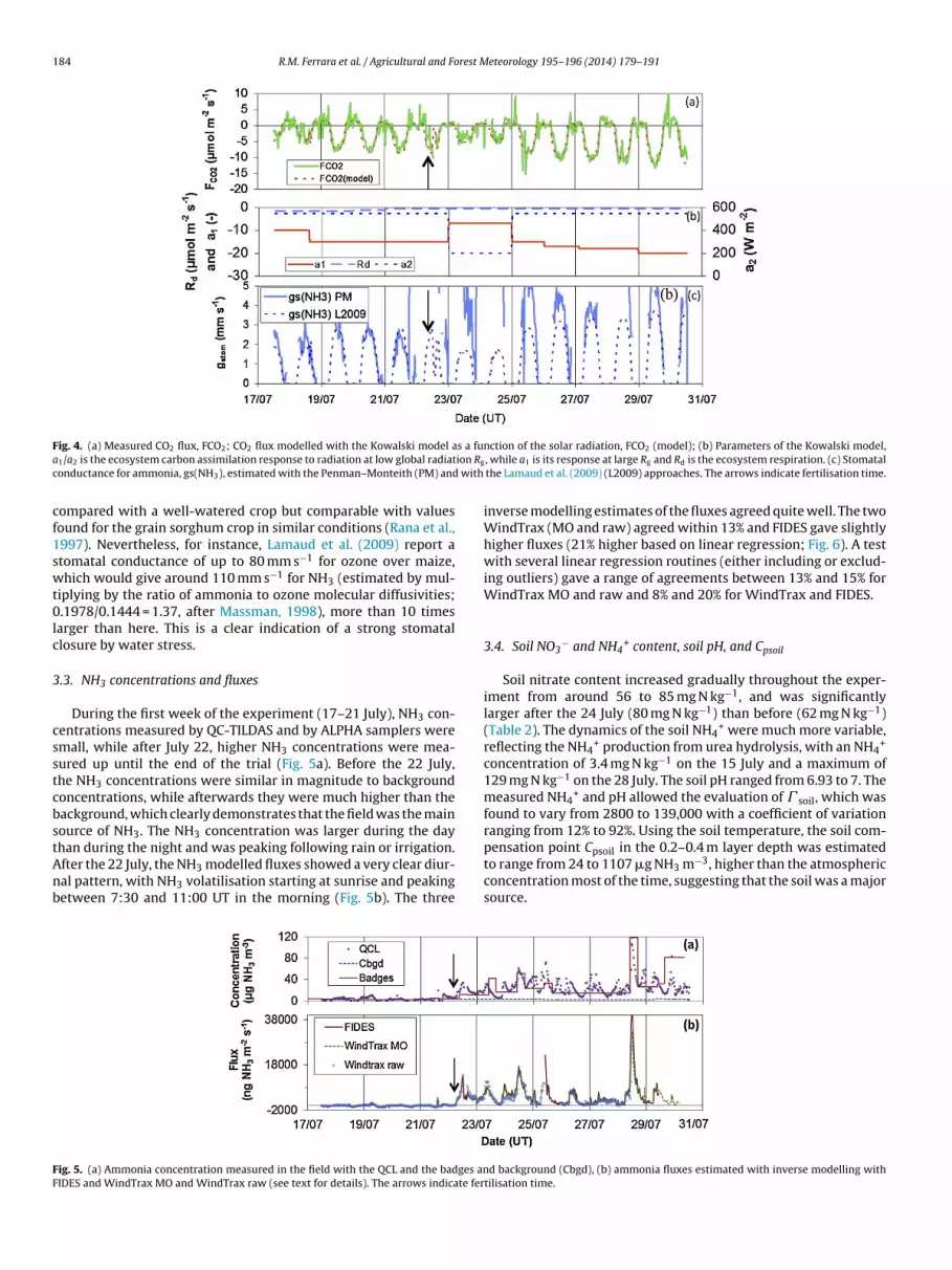

184 R.M. Ferrara et al. / Agricultural and Forest Meteorology 195–196 (2014) 179–191

F s a fua ion Rg

c with

cf1swt0lc

3

csstcbstAnb

FF

ig. 4. (a) Measured CO2 flux, FCO2; CO2 flux modelled with the Kowalski model a1/a2 is the ecosystem carbon assimilation response to radiation at low global radiatonductance for ammonia, gs(NH3), estimated with the Penman–Monteith (PM) and

ompared with a well-watered crop but comparable with valuesound for the grain sorghum crop in similar conditions (Rana et al.,997). Nevertheless, for instance, Lamaud et al. (2009) report atomatal conductance of up to 80 mm s−1 for ozone over maize,hich would give around 110 mm s−1 for NH3 (estimated by mul-

iplying by the ratio of ammonia to ozone molecular diffusivities;.1978/0.1444 = 1.37, after Massman, 1998), more than 10 times

arger than here. This is a clear indication of a strong stomatallosure by water stress.

.3. NH3 concentrations and fluxes

During the first week of the experiment (17–21 July), NH3 con-entrations measured by QC-TILDAS and by ALPHA samplers weremall, while after July 22, higher NH3 concentrations were mea-ured up until the end of the trial (Fig. 5a). Before the 22 July,he NH3 concentrations were similar in magnitude to backgroundoncentrations, while afterwards they were much higher than theackground, which clearly demonstrates that the field was the mainource of NH3. The NH3 concentration was larger during the day

han during the night and was peaking following rain or irrigation.fter the 22 July, the NH3 modelled fluxes showed a very clear diur-al pattern, with NH3 volatilisation starting at sunrise and peakingetween 7:30 and 11:00 UT in the morning (Fig. 5b). The three

ig. 5. (a) Ammonia concentration measured in the field with the QCL and the badges anIDES and WindTrax MO and WindTrax raw (see text for details). The arrows indicate fer

nction of the solar radiation, FCO2 (model); (b) Parameters of the Kowalski model,, while a1 is its response at large Rg and Rd is the ecosystem respiration. (c) Stomatal

the Lamaud et al. (2009) (L2009) approaches. The arrows indicate fertilisation time.

inverse modelling estimates of the fluxes agreed quite well. The twoWindTrax (MO and raw) agreed within 13% and FIDES gave slightlyhigher fluxes (21% higher based on linear regression; Fig. 6). A testwith several linear regression routines (either including or exclud-ing outliers) gave a range of agreements between 13% and 15% forWindTrax MO and raw and 8% and 20% for WindTrax and FIDES.

3.4. Soil NO3− and NH4

+ content, soil pH, and Cpsoil

Soil nitrate content increased gradually throughout the exper-iment from around 56 to 85 mg N kg−1, and was significantlylarger after the 24 July (80 mg N kg−1) than before (62 mg N kg−1)(Table 2). The dynamics of the soil NH4

+ were much more variable,reflecting the NH4

+ production from urea hydrolysis, with an NH4+

concentration of 3.4 mg N kg−1 on the 15 July and a maximum of129 mg N kg−1 on the 28 July. The soil pH ranged from 6.93 to 7. Themeasured NH4

+ and pH allowed the evaluation of � soil, which wasfound to vary from 2800 to 139,000 with a coefficient of variationranging from 12% to 92%. Using the soil temperature, the soil com-

pensation point Cpsoil in the 0.2–0.4 m layer depth was estimatedto range from 24 to 1107 �g NH3 m−3, higher than the atmosphericconcentration most of the time, suggesting that the soil was a majorsource.

d background (Cbgd), (b) ammonia fluxes estimated with inverse modelling withtilisation time.

R.M. Ferrara et al. / Agricultural and Forest Meteorology 195–196 (2014) 179–191 185

Table 2Soil ammonium [NH4

+] and nitrate [NO3−] concentration, soil pH (measured in KCl), soil water content and temperature in the 0.2–0.4 m depth layer, apoplastic [NH4

+]/[H+]ratio (� ), soil compensation point (Cpsoil), the averaged NH3 flux during the given day, and the cumulated NH3 losses during the period between one soil sampling and thenext. Either the standard deviation (±) or the coefficient of variation (%) is given.

Date [NH4+] [NO3

−] pH in KCl (–) water content(%)

� soil (–) Tsoil (0–10 cm)(◦C)

Cpsoil

(�g NH3 m−3)NH3 fluxes(g N ha−1 day−1)

NH3 lossescumulated(g N ha−1)

(mg N kg−1 dry soil)

15/07/2008 3.4 ± 0.7 56.4 ± 11.3 7.00 ± 0.20 10.4 2810 (23%) 26.4 ± 0.7 24 (23%) – –18/07/2008 57.0 ± 32.3 62.5 ± 18.4 6.93 ± 0.18 10.3 40,160 (59%) 26.4 ± 0.7 336 (59%) 143 ± 260 0.1522/07/2008 39.8 ± 14.1 66.3 ± 10.4 7.03 ± 0.18 9.0 35,000 (37%) 26.9 ± 1.2 281 (37%) 2801 ± 2317 2.324/07/2008 105.3 ± 95.7 82.0 ± 14.8 7.05 ± 0.05 15.5 97,000 (92%) 25.3 ± 1.4 526 (92%) 5616 ± 3973 8.728/07/2008 128.7 ± 65.1 73.3 ± 39.6 7.12 ± 0.04 9.7 139,000 (51%) 24.3 ± 1.3 1107 (51%) 7150 ± 9838 19.331/07/2008 46.5 ± 5.0 85.4 ± 41.0 7.13 ± 0.12 8.4 5

Fig. 6. Comparison of ammonia fluxes: FIDES, WindTrax-raw as a function ofWindTrax-MO. Regression lines are: FIDES–y = 1.21x, R2 = 0.97, and WindTrax-r

3

ivtb1

msTiCbl�w

3

mo�Jt

aw–y = 0.87x, R2 = 0.87.

.5. NH3 compensation points

The canopy compensation point C(z0 + d) was estimated bynverse resistance modelling as shown in Eq. (7). This led to aariable � (z0 + d) during the day, with a smaller value at noonhan during the night. Moreover, � (z0 + d) was smaller on averageefore the 22 July than afterwards (Fig. 7). On average, C(z0 + d) was31 �g NH3 m−3 during the highest emission period (22–30 July).

The soil compensation point was also estimated through directeasurements of [NH4

+] and [H+] in the soil (Table 2). The corre-ponding � soil was found to be always larger than the � (z0 + d).his is expected since we have observed NH3 emissions dur-ng this campaign, hence, the concentration at the soil surfacesoil should be larger than C(z0 + d) because of the resistancesetween the two points (see Fig. 2). Similarly C(zm) should be

ower than C(z0 + d). The � soil pattern was the same with a smaller during the first week and a larger one during the secondeek.

.6. Modelled NH3 fluxes by resistance analogy

A two-layer resistance model is useful for interpreting the esti-ated fluxes and for analysing whether the fluxes are due to soil

r plant emissions. If the stomatal flux is set to zero and thesoil is set to the measured values of Table 2 (except on the 18

uly as we suspect contamination), we see that the dynamics ofhe modelled flux follow the flux dynamics estimated by inverse

1,000 (12%) 25.5 ± 0.8 319 (12%) 3256 ± 7504 22.4

modelling (Fig. 8a) quite well. In particular the flux dynamic isquite well represented with a daily pattern showing small fluxes atnight and large flux during the day. This indicates that the observeddaily pattern is principally driven by the aerodynamic resistances(above and within the canopy, Fig. 2) and soil surface temperature(which drives Csoil via the Henry constant). However, the modelledflux with the sole soil source tends to overestimate afternoon andearly night NH3 fluxes, especially on the 23, 26, 27 and 29 July,which could be due to a decreasing availability of NH4

+ in thesoil due to volatilisation (a process not taken into account in themodel). Finally, the soil emission model does not reproduce thelarge volatilisation peaks observed on the 24, 25 and 28 July. Thesedates correspond to irrigation or rain events which must have led toa sudden release of urea and therefore NH4

+ in the soil, for whichthe dynamics can be quick (Roelcke et al., 2002; Sommer et al.,2004). These peaks may also partly be explained by NH3 release bythe cuticles following night time adsorption, an assumption that isfurther discussed in the following section.

In the second test, the soil flux was forced to zero and thestomatal emission potential � stom was set to � soil which wouldcorrespond to � values much larger than reported values (up to10 times larger in the review of Massad et al., 2010). Despite thelarge � stom, the NH3 flux was much smaller than the modelled oneif only stomata are considered, except towards the end of the mea-surement campaign, both because of the large � and the increasedstomatal conductance (Figs. 4c and 8b). Additionally, the night-timeflux goes to zero as the stomata closed.

The “optimised” or fit model was constructed to best repro-duce the daily dynamics of the NH3 flux by adjusting � soil inresponse to rain and irrigation events as explained in the materialand methods (Fig. 8c). This parameterisation allowed reproducingthe measured fluxes quite satisfactorily (Fig. 8c). A value of � = 0.72and � stom = 92,300 best reproduced the observations after the 22July. The optimised � soil after each rain/irrigation event were foundto be 90,500 the 22 July, 126,600 the 23 July, 219,300 the 24 July,766,200 the 25 July and 744,400 the 28 July. The linear regressionbetween modelled and measured fluxes gives a slope of 0.97 andan r2 of 0.48. The RMSE was however high (2.91 �g NH3 m−2 s−1)which represents 96% of the averaged measured flux. The modelledcumulated flux was 9% smaller than the measured one. Althoughthe model roughly reproduces the flux dynamics, the high RMSEand small r2 demonstrate that large differences still exist: the largeremission peaks are not well reproduced (on 24 and 28 July) and themodel often overestimates afternoon fluxes (Fig. 8c). These differ-ences could be explained by the dynamics of NH4

+ availability andwater content in the soil surface layers which are not taken into

account in the current approach and which are discussed later on.Nevertheless, with this parameterisation, the soil dominates theflux while the stomatal and cuticular fluxes are small and of thesame magnitude (Fig. 8e).

186 R.M. Ferrara et al. / Agricultural and Forest Meteorology 195–196 (2014) 179–191

1000

10000

100000

1000000

17/07 19 /07 21 /07 23 /07 25 /07 27 /07 29 /07 31 /07

(z0)

, so

il

Date

Micromet (z0)

Soil

F flux

s lets. T

4

4u

bLTwth

F�s

ig. 7. Emission potential estimated from soil NH4+ and pH (� soil = “Soil”), and from

hade on the 18 July because we suspect a contamination of the sample by urea pel

. Discussion

.1. Flux estimated with inverse modelling and associatedncertainties

Inverse modelling methods to estimate ground emissions haveeen long used both with Gaussian-like models and backwardagrangian stochastic (bLS) dispersion models (Flesch et al., 1995).

he methodology has been proven to be robust (Flesch et al., 2004)orking even with disturbed flow (Flesch et al., 2005a), thanks to

he work initiated by Thomas K. Flesch and John D. Wilson thatas led to the development of WindTrax. However, both LS and

ig. 8. Comparison of measured fluxes (estimated by inverse modelling) and those modesoil from Table 2, (b) no soil flux and � stom assumed equal to � soil in Table 2, (c) optimise

tomatal and cuticular fluxes are given. Left axis in (e) is cuticular flux. The arrows indica

inversion (� (z0 + d) = “Micromet (z0)). The soil measured � soil is shown in a lighterhe arrow indicates fertilisation time.

Gaussian-like models have been shown to be adapted for estimat-ing emissions from fields (Carozzi et al., 2013c; Flesch et al., 2004;Gao et al., 2009; Loubet et al., 2010) and farm buildings (Flesch et al.,2005b; Hensen et al., 2009; McGinn et al., 2006, 2007; Sommeret al., 2005). Excluding extreme stability conditions, bLS models areon average less than 2% biased even in disturbed flows but with avariability of around 20% between trials (Flesch et al., 2004, 2005a).Under unstable conditions the bLS method tends to underestimate

the source strength by up to 30%, while it may overestimate it byup to 40% under stable conditions (Gao et al., 2009). Eulerian mod-els like FIDES have also been shown to be almost unbiased whencompared to gradient methods (less than 7%) (Loubet et al., 2010),

lled by resistance analogy with several parameterisations: (a) no stomatal flux andd � soil and � stom. In (d) the optimised � soil and � stom are shown and in (e) the soil,te fertilisation time.

rest M

oeFpWu

pwa2eFld

eoudttfiiatiob2suttmhCwliNo

eeccdageta2

4

aNiAuaeJ

R.M. Ferrara et al. / Agricultural and Fo

r when compared to bLS models (Carozzi et al., 2013c). Carozzit al. (2013b) have further shown that the differences betweenIDES and WindTrax were due to dissimilarities in eddy diffusivityarameterisation which cause FIDES to give larger estimates thanindTrax under slightly unstable conditions and smaller estimates

nder slightly stable conditions.In this study the FIDES and the WindTrax model (with two

arameterisations WindTrax-MO and WindTrax-raw) comparedell in estimating NH3 emission from the urea-treated field with

bias of 21% (R2 = 0.97) between WindTrax-MO and FIDES and2% (R2 = 0.82) between WindTrax-raw and FIDES (based on lin-ar regression with imposed intercept at 0, see Figs. 5b and 6).IDES gives on average larger estimates than WindTrax, becausearger fluxes occur during unstable conditions during which eddyiffusivity in FIDES is larger than in WindTrax (Carozzi et al., 2013c).

It is crucial to understand that inverse modelling methodsssentially evaluate the emission flux that would explain thebserved concentration increase above a well-localised source areander the measured turbulent regime. These methods are highlyependent upon the fact that the source is isolated and its geome-ry is well known, which was the case here (Fig. 1). They also requirehat the concentration difference between the measurement in theeld and the background (Cbgd) is correctly measured, which is eas-

er if the concentration difference is large, and which was the casefter the 22 July (Fig. 5a). However, the background concentra-ion was measured with badges over weekly periods, whereas its expected that Cbgd has a daily pattern due to the combinationf the variation of background sources with temperature and theoundary layer height variation throughout the day (Hensen et al.,009). The pattern of Cbgd will also be dependent on whether NH3ources are rather localised or more remote and diffuse. To eval-ate the potential impact of such a variability we have assumedhat Cbgd either (1) varied as a function of temperature, followinghe Henry equilibrium, or (2) had a similar daily pattern as C(zm), to

imic the boundary layer height effect on concentration. In the twoypotheses, the average Cbgd was conserved and equal to measuredbgd. Hypothesis (1) leads to very similar fluxes as those estimatedith the measured background concentration, while hypothesis (2)

eads to a much smaller NH3 flux during the first week of the exper-ment with almost no deposition. However, after the 22 July, whenH3 volatilisation starts, the Cbgd daily pattern has negligible effectn the flux (data not shown).

Finally inverse dispersion methods also require a good param-terisation of the turbulence in the surface layer. To evaluate theffect of such parameterisation on the estimated NH3 flux, we haveompared WindTrax-raw which is based on measured turbulenceharacteristics, and WindTrax-MO and FIDES which are used in twoifferent parameterisations of the turbulence in the surface bound-ry layer. The fact that the three models agree within roughly 20%ives confidence in the robustness of these estimates of the NH3mission, especially after the 22 July. We can therefore concludehat the inverse dispersion model gives a robust estimate of themmonia flux and that the method has an uncertainty lower than0%.

.2. Dynamics of NH3 volatilisation following urea application

As reported by Sommer et al. (2004), NH3 emission from soil-pplied fertilizers is controlled by the equilibrium between theH4

+ in the soil solution and the NH3 present in the atmosphere. Asnorganic fertilizers, like urea, do not contain ammoniacal N (Totalmmoniacal N (TAN) = NH3 + NH4

+), NH3 is not emitted until the

rea is hydrolysed, which requires adequate moisture conditionsround the urea grains. This hydrolysis phase explains why no NH3mission was observed following the urea application on the 16uly until irrigation occurred (Table 2 and Fig. 8c). Indeed, NH3

eteorology 195–196 (2014) 179–191 187

volatilisation started immediately following irrigation and reacheda maximum 7 days later on the 22 July. These results are in agree-ment with Roelcke et al. (2002): they found that NH3 fluxes began toincrease on the fourth day after urea spreading on winter wheat andreached a maximum after 7–8 days under humid conditions, whileunder dry conditions the maximum was observed 11 days after fer-tilisation, since the dry soil surface delayed the diffusion of urea tozones of high urease activity and therefore reduced or preventedhydrolysis. Following the application of urea during summer onmaize, Roelcke et al. (2002) observed that NH3 volatilisation startedon the day of spreading, in sharp contrast with the results from lab-oratory experiments where at least 2 days of favourable conditionsfor urea hydrolysis were necessary for substantial NH3 losses tooccur. Sanz-Cobena et al. (2008) found that NH3 losses reached amaximum 4 days after urea application.

It is likely that hydrolysis started after the irrigation on themorning of 22 July, which was the first significant water supplyfollowing the urea application on 16 July. This hypothesis is sup-ported by the observed increase in soil NH4

+ concentration, whichrose from 3.4 mg kg−1 of dry soil on the 15 July to 105 mg kg−1 ofdry soil on the 23 July (see Table 2). The pH also increased whichmay be explained by the ammonium release in the soil (Black et al.,1985).

4.3. Compensation point and emission potential

The � soil, which was determined by in situ measurements ofNH4

+ and pH, ranged from around 3000 to around 140,000, andaveraged 80,500 between the 22 and the 30 July, a value in agree-ment with measurements reported by Sutton et al. (2009a,b) forammonium nitrate application (� soil ranging from 10,000 to morethan 100,000: David et al. (2009) reported a value of 105,000). TheNH4

+ concentration measured in the soil is comparable to what Liand Wang (2008) reported for urea application, but much higherthan what Sanz-Cobena et al. (2008) found for Mediterranean con-ditions in a comparable soil (maximum 20 mg N kg−1), although theNO3

− concentration they report is similar to this study (from 30 to60 mg N kg−1). The � soil estimated by Sanz-Cobena et al. (2008)would however be much higher than what we found here due toa soil pHH2O of 8.1 in their study. Indeed, we estimated a � soil of264,000 for their study, with a soil density of 1470 kg m−3, and a soilNH4

+ concentration of 20 mg N kg−1. Similarly the estimated � soilin Li and Wang (2008) was 247,000 (using pHKCl = 6.99, a soil densityof 1118 kg m−3, and a soil NH4

+ concentration of 300 mg N kg−1).However, the optimised � soil which best reproduces the observedNH3 fluxes showed much higher peaks, up to 766,200 on the 25 and28 July (Fig. 8d). The higher values of � soil required to reproducethe measured NH3 flux can be explained by the fact that � soil in themodel is considered at the soil surface while the measured � soil isbetween 0.2 and 0.4 m depth. The peaks parameterised in Fig. 8are justified as the surface � soil will be much larger than that at0.2–0.4 depth when the urea is dissolved and hydrolysed and willthen decrease quickly as NH3 volatilises and NH4

+ is transferredfurther down in the soil or immobilised (Génermont and Cellier,1997). The optimised � soil averaged 104,200 from 22 to 30 July,a value much more in the range of values found by Sanz-Cobenaet al. (2008) and Li and Wang (2008) and on the higher end of whatSutton et al. (2009a,b) report. We can conclude that the � soil mea-sured in this study was in the range of the reported � soil for ureaand ammonium nitrate applications.

The resistance modelling approach led to a � (z0 + d) averaging4800 before the 22 July and 29,200 afterwards. These measure-

ments give an estimate of the compensation point of the wholecanopy, and hence aggregate soil emissions and deposition to oremission from the canopy. The � (z0 + d) before 22 July (Fig. 7) com-pares rather well with the stomatal � stom proposed by Massad et al.

188 R.M. Ferrara et al. / Agricultural and Forest Meteorology 195–196 (2014) 179–191

05

101520253035

17/07 22/07 27/07 01/08 06/08C

umul

ated

flux

(kg

N-N

H3

ha- 1

)Date (UT)

FIDESExtr apolat ed res istance model

Fig. 9. Cumulated ammonia volatilisation during the experimental period (17–30 July 2008). The total amount of ammonia volatilised is equal to 9.9% of the total N applieda llowiv

(rnte(tat�

4

jceattteee

TE

R

nd 10.7% of the N applied after the 16 July. An evaluation of the volatilisation foolatilised). The arrow indicates fertilisation time.

2010) (� stom = 2603, for 210 kg N ha−1), but is smaller than thoseeported by Loubet et al. (2009) for maize supplied with ammoniumitrate (� stom = 10,000, for 150 kg N ha−1). However the parame-erised � stom (Fig. 8d) was very close to the one proposed by Massadt al. (2010) before 22 July (2800) but much larger after 22 July92,300). The hypothesis of assimilation and hydrolysis of urea byhe plant is possible (Witte, 2011) and would justify the high � stom

fter the 22 July. Although the � stom was high, NH3 was depositedo the plant because � soil was most of the time larger than

stom.

.4. Morning peak ammonia emissions

A peak in NH3 emission was often observed in the morning,ust after sunrise especially on the 25, 27 and 29 July (Fig. 8a and). This peak could not be explained by stomatal emissions or soilmissions (Fig. 8a and b). Because of the large NH3 concentrationst night after the 22 July, we hypothesise that NH3 is deposited onhe wet cuticle at night and re-emitted when water evaporates. Inhe morning, when water evaporates, or if the NH3 concentration in

he atmosphere decreases, the NH3 deposited on the cuticle may bemitted back to the atmosphere (Burkhardt et al., 2009; Flechardt al., 1999). A similar uneven emission pattern (with largermission in the morning) was also observed over cut grassland in

able 3xamples of NH3 losses following urea application expressed as a percentage of the nitro

Fertilizer and technique Method % loss

Laboratory measurements Flow-throughchamber technique

62–70%,

Broadcast application of urea REA 0.8%

Broadcast application of urea Vented chamber 7.0%

Broadcast application of urea Vented chamber 4.8–5.6%

Broadcast application IHF 25–48%

Broadcast application followed byincorporation

IHF 18.0%

Deep point placement IHF 11–12%

Urea solution on moist soil IHF 4–20%

Broadcast application with 10 mm irrigation IHF 10.1%

Broadcast application with 10 mm irrigationand NBTP inhibitor

IHF 5.9%

Broadcast application at several stages of Ricegrowth

Range of methods 5.5–23.5%

Broadcast application Wind tunnel 28.4–29.5%

Broadcast application with 4 mm irrigation bLS 29.0%

Broadcast application Vented chamber 2.1–9.5%

Broadcast application IHF 15–20%

Broadcast application and incorporation IHF 0.5–2.3%

Broadcast application of urea Inverse modelling 9.7%a

EA stands for Relaxed Eddy accumulation. IHF stands for Inverse Horizontal Flux. bLS staa % of total application of nitrogen (240 kg N ha−1). If the period after the 30 July is estimb GS stands for growing season.

ng the experimental period with the resistance model is also shown (13.8% of N

the GRAMINAE experiment (Personne et al., 2009; Sutton et al.,2009a). During this period the NH3 emission was concluded tocome mainly from the litter decomposition. The model usedto compare with the measured fluxes failed to reproduce thispattern correctly, just as in this study (Sutton et al., 2009a).Emission from the cuticle exists potentially, but is not frequentlyobserved (Flechard et al., 1999). However, the very dry conditionsencountered in Mediterranean climate may lead to a high saltconcentration in the dew or directly on the leaf surface becauseof the dust load. These salts promote water adsorption on theleaf at relative humidity lower than saturation (typically 70%)(Burkhardt, 2010; Burkhardt and Eiden, 1994; Burkhardt et al.,2009). The mechanism of NH3 volatilisation from cuticles couldbe explained by the Sechenov relation: at moderately low saltconcentration (below 5000 mol m−3), the solubility of gases expo-nentially decreases when salt concentration increases in water,hence when water evaporates (Weisenberger and Schumpe, 1996).This would lead to an increased compensation point comparedwith the standard Henry constant approach, which may explainsome of the observed emission peaks in the morning.

Morning emission peaks may also be explained by night-timerewetting of the soil surface by dew and capillarity. The urea pelletswould then have been dissolved which would have then releasednitrogen at the soil surface.

gen applied, for different crops using several methods.

% lossaveraged

No. daysb Crop Reference

66.0% 38 Soil incubation Akiyama et al. (2004)

0.8% 23 Maize Zhu et al. (2000)7.0% 80 Maize Wang et al. (2004)5.2% GS Maize Roelcke et al. (2002)

36.0% 8–15 Maize Pacholski et al. (2006)18.0% 8–15 Maize Pacholski et al. (2006)

11.5% 8–15 Maize Pacholski et al. (2006)13.7% 9 Bare soil McInnes et al. (1986)10.1% 38 Sunflower Sanz-Cobena et al. (2008)

5.9% 38 Sunflower Sanz-Cobena et al. (2008)

15.0% - RICE Yan et al. (2003)(reviewing several authors)

29.0% 7 Grass van der Weerden and Jarvis(1997)

29.0% 6 Dry prairie Sommer et al. (2005)6.0% GS Winter wheat Wang et al. (2004)

17.5% 8–15 Winter wheat Pacholski et al. (2006)1.6% 8–15 Winter wheat Pacholski et al. (2006)9.7% 14 Grain sorghum Present study

nds for backward Lagrangian Stochastic Model.ated, the percentage becomes 13.2%.

rest M

4

itcahpeus

ladeac3

tAtTrwfof2Wtt

5

•

•

•

••

•

•

A

“2ibEFBPia

R.M. Ferrara et al. / Agricultural and Fo

.5. Cumulated NH3 losses

The NH3 volatilisation clearly started on the 22 July afterrrigation (Fig. 9). The total amount lost was 23.2 kg N ha−1 overhe 14 days of the campaign. The typical sigmoid trend in the NH3umulated loss described by a Michaelis–Menten equation is notpplicable to our data (Fig. 9). In fact, only two of the three phasesave been observed in our trial: the onset of urea hydrolysis, thehase of increasing NH3 emissions, but not the phase of decreasingmissions. It is therefore very likely that the NH3 emission contin-ed following the end of the experimental campaign, which wastopped prematurely due to instrument breakdown.

In order to evaluate the missing NH3 emissions, we have simu-ated the emissions from 30 July to 10 August using the resistancepproach, assuming that the soils emission potential graduallyecreased within 10 days to reach the value measured before thexperiment, and further assuming the NH3 concentration in thetmosphere decreased similarly. This simulation showed that theumulated NH3 emission during that period could represent up to6% of the emission measured before the 30 July.

The amount of NH3 lost by volatilisation during the experimen-al period corresponded to 9.9% of the total applied nitrogen (TAN).ccounting for ammonia emissions that would have occurred after

he experiment would lead to an emission factor of 13.8% TAN.hese NH3 emissions are very similar, though smaller than thoseeported by Sanz-Cobena et al. (2008) for a very comparable soilith similar wetness (Table 3). Overall the NH3 emission factor

ound here is in the range of those reported for urea applicationver a variety of crops (Table 3). Usually lower emissions are foundor dryer soils than wetter ones (Sommer et al., 2004; Meyers et al.,006; Sutton et al., 2000; Yamulki et al., 1996; Zhu et al., 2000).e can conclude that the cumulated loss at our arid site was in

he range of reported losses following urea application, and closeo those reported for similar soil and meteorological conditions.

. Conclusions

Ammonia volatilisation was measured following urea applicationto a sorghum field in semi-arid conditions.Under such conditions, the sorghum did not show any sign ofwater stress.Ammonia volatilisation started immediately following irrigation,and the maximum volatilisation flux was reached 7 days later.The ammonia fluxes ranged from −2.5 to 45 �g NH3 m−2 s−1.After urea hydrolysis, the canopy compensation point reached131 �g NH3 m−3, while the soil compensation point averaged800 �g NH3 m−3.The soil was therefore clearly identified as the main source ofNH3.The ammonia emission factor ranged between 10% and 14% of thetotal applied nitrogen.

cknowledgments

This study has been supported by Italian Projects FISRCLIMESCO” (DD 285/ric 2/2/2006) and AQUATER (DM n.09/7303/05). European Project NitroEurope supported the exper-

mental field work. The corresponding author has been also fundedy NinE – ESF Research Networking Programme “Nitrogen inurope” and ACCENT – Biaflux (Network of Excellence funded by EC,P6, PRIORITY 1.1.6.3 Global Change and Ecosystems: subproject

iosphere-Atmosphere Exchange of Pollutants). The authors thankasquale Introna and Nicola Martinelli for them helping in conduct-ng the experimental work in the field and Marcello Mastrangelond Dr. Carola Vitti for laboratory measurements. The authors thank

eteorology 195–196 (2014) 179–191 189

Dr. David Nelson from Aerodyne Res. for his support on the fastammonia analyzer. The authors thank the associate editor TimothyJ Griffis and the reviewers for their comments that greatly helpedimproving the manuscript. They also thank Polina Voylokov for hercareful correction of the revised manuscript.

References

Akiyama, H., McTaggart, I., Ball, B., Scott, A., 2004. N2O, NO, and NH3 emissions fromsoil after the application of organic fertilizers, urea and water. Water Air SoilPollut. 156 (1), 113–129.

Aubinet, M., Grelle, A., Ibrom, A., Rannik, U., Moncrieff, J., Foken, T., Kowalski, A.S.,Martin, P.H., Berbigier, P., Bernhofer, C., Clement, R., Elbers, J., Granier, A., Grun-wald, T., Morgenstern, K., Pilegaard, K., Rebmann, C., Snijders, W., Valentini,R., Vesala, T., 2000. Estimates of the annual net carbon and water exchange offorests: the EUROFLUX methodology. Adv. Ecol. Res. 30, 113–175.

Black, A.S., Sherlock, R.R., Cameron, K.C., Smith, N.P., Goh, K.M., 1985. Comparisonof 3 field methods for measuring ammonia volatilization from urea granulesbroadcast on to pasture. J. Soil Sci. 36 (2), 271–280.

Brodeur, J.J., Warland, J.S., Staebler, R.M., Wagner-Riddle, C., 2009. Technical note:laboratory evaluation of a tunable diode laser system for eddy covariance mea-surements of ammonia flux. Agric. For. Meteorol. 149 (2), 385–391.

Burkhardt, J., Eiden, R., 1994. Thin water films on coniferous needles. Atmos. Environ.28 (12), 2001–2017.

Burkhardt, J., Flechard, C.R., Gresens, F., Mattsson, M., Jongejan, P.A.C., Erisman,J.W., Weidinger, T., Meszaros, R., Nemitz, E., Sutton, M.A., 2009. Modelling thedynamic chemical interactions of atmospheric ammonia with leaf surface wet-ness in a managed grassland canopy. Biogeosciences 6 (1), 67–84.

Burkhardt, J., 2010. Hygroscopic particles on leaves: nutrients or desiccants? Ecol.Monogr. 80 (3), 369–399.

Carozzi, M., Ferrara, R.M., Rana, G., Acutis, M., 2013a. Evaluation of mitigation strate-gies to reduce ammonia losses from slurry fertilisation on arable lands. Sci. TotalEnviron. 449, 126–133.

Carozzi, M., Loubet, B., Acutis, M., Rana, G., Ferrara, R.M., 2013b. Inverse disper-sion modelling highlights the efficiency of slurry injection to reduce ammonialosses by agriculture in the Po Valley (Italy). Agric. For. Meteorol. 171,306–318.

Carozzi, M., Loubet, B., Acutis, M., Rana, G., Ferrara, R.M., 2013c. Inverse dispersionmodelling highlights the efficiency of slurry injection to reduce ammonia lossesby agriculture in the Po Valley (Italy). Agric. For. Meteorol. 171–172 (0), 306–318.

Das, P., Kim, K.-H., Sa, J.-H., Bae, W.S., Kim, J.-C., Jeon, E.-C., 2008. Emissions of ammo-nia and nitric oxide from an agricultural site following application of differentsynthetic fertilizers and manures. Geosci. J. 12 (2), 177–190.

David, M., Loubet, B., Cellier, P., Mattsson, M., Schjoerring, J.K., Nemitz, E., Roche,R., Riedo, M., Sutton, M.A., 2009. Ammonia sources and sinks in an intensivelymanaged grassland canopy. Biogeosciences 6 (9), 1903–1915.

Dyer, A.J., Hicks, B.B., 1970. Flux-profile relationship in the constant flux layer. Q.J.R.Meteorol. Soc. 96, 715–721.

ECETOC, 1994. NH3 Emissions to air in Western Europe. Technical report No.62. European Centre for Ecotoxicology and Toxicology of Chemicals, Brussels,Belgium, pp. 196.

Ellis, R.A., Murphy, J.G., Pattey, E., van Haarlem, R., O’Brien, J.M., Herndon, S.C., 2010.Characterizing a Quantum Cascade Tunable Infrared Laser Differential Absorp-tion Spectrometer (QC-TILDAS) for measurements of atmospheric ammonia.Atmos. Measure. Technol. 3 (2), 397–406.

EMEP/EEA and guidebook, 2013. EMEP/EEA Air Pollutant Emission Inventory Guide-book 2013. European Environment Agency, Publications Office of the EuropeanUnion, Luxembourg.

Famulari, D., Fowler, D., Hargreaves, K., Milford, C., Nemitz, E., Sutton, M.A., Weston,K., 2004. Measuring eddy covariance fluxes of ammonia using tunable diodelaser absorption spectroscopy. Water Air Soil Pollut. Focus 4, 151–158.

Famulari, D., Fowler, D., Nemitz, E., Hargreaves, K.J., Storeton-West, R.L., Rutherford,G., Tang, Y.S., Sutton, M.A., Weston, K.J., 2009. Development of a low-cost systemfor measuring conditional time-averaged gradients of SO2 and NH3. Environ.Monit. Assess. 161, 11–27.

Ferrara, R.M., Loubet, B., Di Tommasi, P., Bertolini, T., Magliulo, V., Cellier, P., Eugster,W., Rana, G., 2012. Eddy covariance measurement of ammonia fluxes: compar-ison of high frequency correction methodologies. Agric. For. Meteorol. 158 (0),30–42.

Flechard, C.R., Fowler, D., 1998. Atmospheric ammonia at a moorland site. II:Long-term surface-atmosphere micrometeorological flux measurements. Q.J.R.Meteorol. Soc. 124 (547), 759–791.

Flechard, C.R., Fowler, D., Sutton, M.A., Cape, J.N., 1999. A dynamic chemical modelof bi-directional ammonia exchange between semi-natural vegetation and theatmosphere. Q.J.R. Meteorol. Soc. 125 (559), 2611–2641.

Flechard, C.R., Spirig, C., Neftel, A., Ammann, C., 2010. The annual ammonia budgetof fertilised cut grassland – Part 2: Seasonal variations and compensation pointmodeling. Biogeosciences 7 (2), 537–556.

Flesch, T.K., Wilson, J.D., Yee, E., 1995. Backward-time Lagrangian stochatic dis-

pertion models and their application to estimate gaseous emissions. J. Appl.Meteorol. 34, 1320–1332.

Flesch, T.K., Wilson, J.D., Harper, L.A., Crenna, B.P., Sharpe, R.R., 2004. Deducingground-to-air emissions from observed trace gas concentrations: a field trial.J. Appl. Meteorol. 43 (3), 487–502.

1 rest M

F

F

F

G

G

G

G

G

G

H

H

K

K

K

L

L

L

L

L

L

L

L

M

M

M

M

90 R.M. Ferrara et al. / Agricultural and Fo

lesch, T.K., Wilson, J.D., Harper, L.A., 2005a. Deducing ground-to-air emissions fromobserved trace gas concentrations: a field trial with wind disturbance. J. Appl.Meteorol. 44 (4), 475–484.

lesch, T.K., Wilson, J.D., Harper, L.A., Crenna, B.P., 2005b. Estimating gas emissionsfrom a farm with an inverse-dispersion technique. Atmos. Environ. 39 (27),4863–4874.

lesch, T.K., Wilson, J.D., Harper, L.A., Todd, R.W., Cole, N.A., 2007. Determiningammonia emissions from a cattle feedlot with an inverse dispersion technique.Agric. For. Meteorol. 144 (1–2), 139–155.

alloway, J.N., Townsend, A.R., Erisman, J.W., Bekunda, M., Cai, Z.C., Freney, J.R.,Martinelli, L.A., Seitzinger, S.P., Sutton, M.A., 2008. Transformation of the nitro-gen cycle: recent trends, questions, and potential solutions. Science 320 (5878),889–892.

ao, X., Giorgi, F., 2008. Increased aridity in the Mediterranean region under green-house gas forcing estimated from high resolution simulations with a regionalclimate model. Global Planet. Change 62 (3–4), 195–209.

ao, Z.L., Mauder, M., Desjardins, R.L., Flesch, T.K., van Haarlem, R.P., 2009.Assessment of the backward Lagrangian Stochastic dispersion technique forcontinuous measurements of CH4 emissions. Agric. For. Meteorol. 149 (9),1516–1523.

énermont, S., Cellier, P., 1997. A mechanistic model for estimating ammoniavolatilization from slurry applied to bare soil. Agric. For. Meteorol. 88 (1–4),145–167.

iardini, A., Vecchietti, M., 2000. In: Pàtron (Ed.), Coltivazioni erbacee: cereali eproteaginose. , pp. 201–220.

raefe, J., 2004. Roughness layer corrections with emphasis on SVAT model appli-cations. Agric. For. Meteorol. 124 (3–4), 237–251.

ensen, A., Loubet, B., Mosquera, J., van den Bulk, W.C.M., Erisman, J.W., Damm-gen, U., Milford, C., Lopmeier, F.J., Cellier, P., Mikuska, P., Sutton, M.A., 2009.Estimation of NH3 emissions from a naturally ventilated livestock farmusing local-scale atmospheric dispersion modelling. Biogeosciences 6 (12),2847–2860.

uijsmans, J.F.M., Hol, J.M.G., Vermeulen, G.D., 2003. Effect of applicationmethod, manure characteristics, weather and field conditions on ammoniavolatilization from manure applied to arable land. Atmos. Environ. 37 (26),3669–3680.

olle, O., Rebmann, C., 2007. EddySoft Documentation of a Software Package toAcquire and Process Eddy Covariance Data. Max-Planck-Institut für Biogeo-chemie.

ormann, R., Meixner, F.X., 2001. An analytical footprint model for non-neutralstratification. Boundary Layer Meteorol. 99 (2), 207–224.

owalski, A.S., Loustau, D., Berbigier, P., Manca, G., Tedeschi, V., Borghetti, M., Valen-tini, R., Kolari, P., Berninger, F., Rannik, U., Hari, P., Rayment, M., Mencuccini, M.,Moncrieff, J., Grace, J., 2004. Paired comparisons of carbon exchange betweenundisturbed and regenerating stands in four managed forests in Europe. GlobalChange Biol. 10 (10), 1707–1723.

amaud, E., Loubet, B., Irvine, M., Stella, P., Personne, E., Cellier, P., 2009. Partitioningof ozone deposition over a developed maize crop between stomatal and non-stomatal uptakes, using eddy-covariance flux measurements and modelling.Agric. For. Meteorol. 149 (9), 1385–1396.

asdon, L.S., Waren, A.D., Jain, A., Ratner, M., 1978. Design and testing of a generalizedreduced gradient code for nonlinear programming. ACM Trans. Math. Softw. 4(1), 34–50.

i, D.J., Wang, X.M., 2008. Nitrogen isotopic signature of soil-released nitric oxide(NO) after fertilizer application. Atmos. Environ. 42 (19), 4747–4754.

oubet, B., Milford, C., Sutton, M.A., Cellier, P., 2001. Investigation of the interactionbetween sources and sinks of atmospheric ammonia in an upland landscapeusing a simplified dispersion-exchange model. J. Geophys. Res. -Atmos. 106(D20), 24183–24195.

oubet, B., Asman, W.A.H., Theobald, M.R., Hertel, O., Tang, Y.S., Robin, P., Hassouna,M., Dammgen, U., Genermont, S., Cellier, P., Sutton, M.A., 2009. Ammonia depo-sition near hot spots: processes, models and monitoring methods. In: Sutton,M.A., Reis, S., Baker, S.M.H. (Eds.), Atmospheric Ammonia. Detecting EmissionChanges and Environmental Impacts. Springer Science + Business Media B.V., pp.205–267.

oubet, B., Cellier, P., Milford, C., Sutton, M.A., 2006. A coupled dispersion andexchange model for short-range dry deposition of atmospheric ammonia. Q.J.R.Meteorol. Soc. 132 (618), 1733–1763.

oubet, B., Génermont, S., Ferrara, R., Bedos, C., Decuq, C., Personne, E., Fanucci, O.,Durand, B., Rana, G., Cellier, P., 2010. An inverse model to estimate ammoniaemissions from fields. Eur. J. Soil Sci. 61, 793–805.

oubet, B., Decuq, C., Personne, E., Massad, R.S., Flechard, C., Fanucci, O., Mascher, N.,Gueudet, J.C., Masson, S., Durand, B., Genermont, S., Fauvel, Y., Cellier, P., 2012.Investigating the stomatal, cuticular and soil ammonia fluxes over a growingtritical crop under high acidic loads. Biogeosciences 9 (4), 1537–1552.

assad, R.S., Nemitz, E., Sutton, M.A., 2010. Review and parameterisation of bi-directional ammonia exchange between vegetation and the atmosphere. Atmos.Chem. Phys. 10 (21), 10359–10386.

assman, W.J., 1998. A review of the molecular diffusivities of H2O, CO2, CH4, CO,O3, SO2, NH3, N2O, NO, AND NO2 in air, O2 and N2 near STP. Atmos. Environ. 32(6), 1111–1127.

cGinn, S.M., Flesch, T.K., Harper, L.A., Beauchemin, K.A., 2006. An approach formeasuring methane emissions from whole farms. J. Environ. Qual. 35 (1), 14–20.

cGinn, S.M., Flesch, T.K., Crenna, B.P., Beauchernin, K.A., Coates, T., 2007. Quan-tifying ammonia emissions from a cattle feedlot using a dispersion model. J.Environ. Qual. 36 (6), 1585–1590.

eteorology 195–196 (2014) 179–191

McInnes, K.J., Ferguson, R.B., Kissel, D.E., Kanemasu, E.T., 1986. Field-measurementsof ammonia loss from surface applications of urea solution to bare soil. Agron.J. 78 (1), 192–196.

McManus, J.B., Shorter, J.H., Nelson, D.D., Zahniser, M.S., Glenn, D.E., McGovern, R.M.,2008. Pulsed quantum cascade laser instrument with compact design for rapid,high sensitivity measurements of trace gases in air. Appl. Phys. B – Lasers Opt.92 (3), 387–392.

Meyers, T.P., Luke, W.T., Meisinger, J.J., 2006. Fluxes of ammonia and sulfateover maize using relaxed eddy accumulation. Agric. For. Meteorol. 136 (3–4),203–213.

Monteny, G.J., Erisman, J.W., 1998. Ammonia emission from dairy cow buildings:a review of measurement techniques, influencing factors and possibilities forreduction. Netherlands J. Agric. Sci. 46 (3–4), 225–247.

Nelson, D.D., McManus, B., Urbanski, S., Herndon, S., Zahniser, M.S., 2004. Highprecision measurements of atmospheric nitrous oxide and methane usingthermoelectrically cooled mid-infrared quantum cascade lasers and detectors.Spectrochim. Acta A – Mol. Biomol. Spectrosc. 60 (14), 3325–3335.

Nemitz, E., Milford, C., Sutton, M.A., 2001. A two-layer canopy compensation pointmodel for describing bi-directional biosphere-atmosphere exchange of ammo-nia. Q.J.R. Meteorol. Soc. 127 (573), 815–833.

Pacholski, A., Cai, G., Nieder, R., Richter, J., Fan, X., Zhu, Z., Roelcke, M., 2006. Calibra-tion of a simple method for determining ammonia volatilization in the field –comparative measurements in Henan Province, China. Nutr. Cycl. Agroecosyst.74 (3), 259–273.

Pain, B.F., Van der Weerden, T.J., Chambers, B.J., Phillips, V.R., Jarvis, S.C., 1998. A newinventory for ammonia emissions from UK agriculture. Atmos. Environ. 32 (3),309–313.

Personne, E., Loubet, B., Herrmann, B., Mattsson, M., Schjoerring, J.K., Nemitz, E.,Sutton, M.A., Cellier, P., 2009. SURFATM-NH3: a model combining the surfaceenergy balance and bi-directional exchanges of ammonia applied at the fieldscale. Biogeosciences 6 (8), 1371–1388.

Philip, J.R., 1959. The theory of local advection: 1. J. Meteorol. 16, 535–547.Rana, G., Katerji, N., Mastrorilli, M., ElMoujabber, M., 1997. A model for predicting

actual evapotranspiration under soil water stress in a Mediterranean region.Theor. Appl. Climatol. 56 (1–2), 45–55.

Raupach, M.R., 1994. Simplified expressions for vegetation roughness length andzero-plane displacement as functions of canopy height and area index. BoundaryLayer Meteorol. 71 (1–2), 211–216.

Raupach, M.R., 1995. Simplified expressions for vegetation roughness length andzero-plane displacement (vol. 71, pg. 211, 1994). Boundary Layer Meteorol. 76(3), 304.

Roelcke, M., Han, Y., Li, S.X., Richter, J., 1996. Laboratory measurements and simu-lations of ammonia volatilization from urea applied to calcareous Chinese loesssoils. Plant Soil 181 (1), 123–129.

Roelcke, M., Li, S.X., Tian, X.H., Gao, Y.J., Richter, J., 2002. In situ comparisons of ammo-nia volatilization from N fertilizers in Chinese loess soils. Nutr. Cycl. Agroecosyst.62 (1), 73–88.

Romano, D., Bernetti, A., Cóndor, R.D., De Lauretis, R., Di Cristofaro, E., Lena, F., Gagna,A., Gonella, B., Pantaleoni, M., Peschi, E., Taurino, E., Vitullo, M., 2013. ItalianEmission Inventory 1990–2011. Informative Inventory Report 2013. ISPRA ––Institute for Environmental Protection and Research Environment Department.

Sanz-Cobena, A., Misselbrook, T.H., Arce, A., Mingot, J.I., Diez, J.A., Vallejo, A., 2008.An inhibitor of urease activity effectively reduces ammonia emissions from soiltreated with urea under Mediterranean conditions. Agric. Ecosyst. Environ. 126(3–4), 243–249.

Schjørring, J.K., 1997. Plant-Atmosphere Ammonia Exchange: Quantification, Physi-ology Regulation and Interaction with Environmental Factors. R. Veterinary andAgric. Univ., Copenhagen, Denmark, pp. 55 (D.Sc. thesis).

Shaw, W.J., Spicer, C.W., Kenny, D.V., 1998. Eddy correlation fluxes of trace gasesusing a tandem mass spectrometer. Atmos. Environ. 32 (17), 2887–2898.

Sintermann, J., Spirig, C., Jordan, A., Kuhn, U., Ammann, C., Neftel, A., 2011. Eddycovariance flux measurements of ammonia by high temperature chemical ion-isation mass spectrometry. Atmos. Measure. Technol. 4 (3), 599–616.

Sintermann, J., Neftel, A., Ammann, C., Häni, C., Hensen, A., Loubet, B., Flechard,C., 2012. Are ammonia emissions from field-applied slurry substantially over-estimated in European emission inventories? Biogeosciences 9, 1611–1632.

Sommer, S.G., Hutchings, N.J., 2001. Ammonia emission from field applied manureand its reduction – invited paper. Eur. J. Agron. 15 (1), 1–15.

Sommer, S.G., Genermont, S., Cellier, P., Hutchings, N.J., Olesen, J.E., Morvan, T., 2003.Processes controlling ammonia emission from livestock slurry in the field. Eur.J. Agron. 19 (4), 465–486.

Sommer, S.G., Schjoerring, J.K., Denmead, O.T., 2004. Ammonia emission from min-eral fertilizers and fertilized crops. Adv. Agron. 82, 82, 557–622.

Sommer, S.G., McGinn, S.M., Flesch, T.K., 2005. Simple use of the backwardsLagrangian stochastic dispersion technique for measuring ammonia emissionfrom small field-plots. Eur. J. Agron. 23 (1), 1–7.

Stella, P., Personne, E., Loubet, B., Lamaud, E., Mascher, N., Cellier, P., 2011. SURFATM-O3: a new model for partitioning ozone deposition over agro-ecosystems.Development and application to a maize canopy, Nitrogen & Global Change.Key Findings – Future Challenges, Edinburgh., pp. 2.

Sutton, M.A., Pitcairn, C.E.R., Fowler, D., 1993. The exchange of ammonia between

the atmosphere and plant communities. Adv. Ecol. Res. 24, 301–389.

Sutton, M.A., Nemitz, E., Milford, C., Fowler, D., Moreno, J., San Jose, R., Wyers, G.P.,Otjes, R.P., Harrison, R., Husted, S., Schjørring, J.K., 2000. Micrometeorologicalmeasurements of net ammonia fluxes over oilseed rape during two vegetationperiods. Agric. For. Meteorol. 105 (4), 351–369.

rest M

S

S

S

T

v

W

R.M. Ferrara et al. / Agricultural and Fo

utton, M.A., Erisman, J.W., Dentener, F., Moller, D., 2008. Ammonia in the environ-ment: from ancient times to the present. Environ. Pollut. 156 (3), 583–604.

utton, M.A., Nemitz, E., Milford, C., Campbell, C., Erisman, J.W., Hensen, A., Cellier,P., David, M., Loubet, B., Personne, E., Schjoerring, J.K., Mattsson, M., Dorsey, J.R.,Gallagher, M.W., Horvath, L., Weidinger, T., Meszaros, R., Dämmgen, U., Neftel,A., Herrmann, B., Lehman, B.E., Flechard, C., Burkhardt, J., 2009a. Dynamics ofammonia exchange with cut grassland: synthesis of results and conclusions ofthe GRAMINAE Integrated Experiment. Biogeosciences 6, 2907–2934.

utton, M.A., Nemitz, E., Theobald, M.R., Milford, C., Dorsey, J.R., Gallagher, M.W.,Hensen, A., Jongejan, P.A.C., Erisman, J.W., Mattsson, M., Schjoerring, J.K., Cel-lier, P., Loubet, B., Roche, R., Neftel, A., Hermann, B., Jones, S.K., Lehman, B.E.,Horvath, L., Weidinger, T., Rajkai, K., Burkhardt, J., Lopmeier, F.J., Daemmgen,U., 2009b. Dynamics of ammonia exchange with cut grassland: strategy andimplementation of the GRAMINAE Integrated Experiment. Biogeosciences 6 (3),309–331.

ang, Y.S., Cape, J.N., Sutton, M.A., 2001. Development and types of passive samplersfor monitoring atmospheric NO2 and NH3 concentrations. ScientificWorldJour-nal 1, 513–529.

an der Weerden, T.J., Jarvis, S.C., 1997. Ammonia emission factors for N fertilizers

applied to two contrasting grassland soils. Environ. Pollut. 95 (2), 205–211.

ang, Z.H., Liu, X.J., Ju, X.T., Zhang, F.S., Malhi, S.S., 2004. Ammonia volatilizationloss from surface-broadcast urea: comparison of vented- and closed-chambermethods and loss in winter wheat-summer maize rotation in North China Plain.Commun. Soil Sci. Plant Anal. 35 (19–20), 2917–2939.

eteorology 195–196 (2014) 179–191 191

Weisenberger, S., Schumpe, A., 1996. Estimation of gas solubilities in salt solutionsat temperatures from 273 K to 363 K. AIChE J. 42 (1), 298–300.

Whitehead, J.D., Twigg, M., Famulari, D., Nemitz, E., Sutton, M.A., Gallagher, M.W.,Fowler, D., 2008. Evaluation of laser absorption spectroscopic techniques foreddy covariance flux measurements of ammonia. Environ. Sci. Technol. 42 (6),2041–2046.

Witte, C.P., 2011. Urea metabolism in plants. Plant Sci.: Int. J. Exp. Plant Biol. 180 (3),431–438.

Yamulki, S., Harrison, R.M., Goulding, K.W.T., 1996. Ammonia surface-exchangeabove an agricultural field in southeast england. Atmos. Environ. 30 (1),109–118.

Yan, X.Y., Akimoto, H., Ohara, T., 2003. Estimation of nitrous oxide, nitric oxide andammonia emissions from croplands in East, Southeast and South Asia. GlobalChange Biol. 9 (7), 1080–1096.

Zahniser, M.S., Nelson, D.D., McManus, J.B., Shorter, J.H., Herndon, S., Jimenez, R.,2005. Development of a Quantum Cascade Laser-Based Detector for NH3 andNitric Acid. Final Report, U.S. Department of Energy, SBIR Phase II, Grant No.DE-FG02-01ER83139.

Zhang, S.L., Cai, G.X., Wang, X.Z., Xu, Y.H., Zhu, Z.L., Freney, J.R., 1992. Losses of urea-

nitrogen applied to maize grown on a calcareous fluvo-aquic soil in North ChinaPlain. Pedosphere 2 (2), 171–178.

Zhu, T., Pattey, E., Desjardins, R.L., 2000. Relaxed eddy-accumulation tech-nique for measuring ammonia volatilization. Environ. Sci. Technol. 34 (1),199–203.