AGGREGATION AND DISAGGREGATION OF STRUCTURAL TIMESERIES MODELS

By Luiz K. Hotta and Klaus L. Vasconcellos

State University of Campinas and University of Pernambuco, Brazil

First version received May 1995

Abstract. The aggregation/disaggregation problem has been widely studied in thetime series literature. Some main issues related to this problem are modelling,prediction and robustness to outliers. In this paper we look at the modelling problemwith particular interest in the local level and local trend structural time series modelstogether with their corresponding ARIMA(0, 1, 1) and ARIMA(0, 2, 2) representations.Given an observed time series that can be expressed by a structural or autoregressiveintegrated moving-average (ARIMA) model, we derive the necessary and suf®cientconditions under which the aggregate and/or disaggregate series can be expressed bythe same class of model. Harvey's cycle and seasonal components models (Harvey,Forecasting, Structural Time Series Models and the Kalman Filter, Cambridge:Cambridge University Press, 1989) are also brie¯y discussed. Systematic sampling ofstructural and ARIMA models is also discussed.

Keywords. Aggregation of time series models; disaggregation of time series models;aggregation of structural time series models; disaggregation of structural time seriesmodels.

1. INTRODUCTION

The aggregation/disaggregation problem has been widely studied in the timeseries literature. Some main issues related to this problem are modelling,prediction and robustness to outliers. We look at the modelling problem, withparticular interest in the local level and local trend structural time series modelstogether with their corresponding ARIMA(0, 1, 1) and ARIMA(0, 2, 2)representations. Given an observed time series that can be expressed by astructural or autoregressive integrated moving-average (ARIMA) model, we givethe conditions under which the aggregate and/or disaggregate series can beexpressed by the same class of model. Most of the work in the literature deals withthe aggregation problem. A survey for the case of aggregation of ARIMA modelscan be found in Pino et al. (1987) (see also Stram and Wei, 1986a). Tiao (1972)studied some cases when the period of aggregation goes to in®nity. Theaggregation of the structural model was considered by Gonzalez (1992, 1993) andHarvey and Stock (1994) using a non-Bayesian approach and by Vasconcellos(1992), using a Bayesian approach, both using the state space modellingformulation. There are also studies on disaggregation (see, for instance, Stram and

0143-9782/99/04 155±171 JOURNAL OF TIME SERIES ANALYSIS Vol. 20, No. 2# 1999 Blackwell Publishers Ltd., 108 Cowley Road, Oxford OX4 1JF, UK and 350 Main Street,Malden, MA 02148, USA.

Wei, 1986b; Guerrero, 1990; Nijman and Palm, 1990; Gonzalez, 1992, 1993;Harvey and Stock, 1994). However, none of the work on aggregation anddisaggregation deals directly with the modelling problem and all the results foundin the literature about structural time series models are derived under theassumption that the model for the basic series is an orthogonal model, anassumption that is necessary for the identi®cation of the parameters. In this paperwe use the relationship between structural and ARIMA models and treat both theaggregation and disaggregation problem for the structural time series models withand without the orthogonality assumption. Section 2 presents the models and givesthe relationship between structural and ARIMA models. Sections 3 and 4 dealwith the problem of temporal aggregation and disaggregation of time series withSection 3 presenting the aggregation and disaggregation of ARIMA and structuralmodels. Since the structural model is widely used in the context of unobservedcomponents models with cyclical and seasonal components (see Harvey (1989)and West and Harrison (1989) for the Bayesian and non-Bayesian approach,respectively), we discuss, in Section 4, the models suggested by Harvey for thesecomponents. Section 5 analyses the systematic sampling of time series. Con-cluding remarks are presented in Section 6.

2. STRUCTURAL AND ARIMA TIME SERIES MODELS

The relationship between structural and ARIMA time series models is alreadywell known. This section only introduces the terminology and notation andreviews the main results that will be used in Section 3.

2.1. Local level structural model

Consider the local level structural model

yt � ì t � å t

ì t � ì tÿ1 � ç t(1)

where å t and ç t are white noise processes with variances equal to ó 2å and ó 2

ç,respectively. Traditionally, å t and ç t are considered to be uncorrelated for allinstants of time. We will consider here that å t and ç t are uncorrelated fordifferent instants of time, but can have a contemporaneous correlation given byr � corr(å t, ç t). Godolphin and Stone (1980) supported this modi®cation on thebasis that this model structure can yield useful polynomial projecting predictors.Here, we will call the structural model with r � 0 the orthogonal or uncorrelatedstructural model, and the general model will be called the non-orthogonal model.It is a well-known result that the class of local level non-orthogonal structuralmodels and the class of ARIMA(0, 1, 1) models are equivalent. From now on,we will refer equivalently to the (general) local level non-orthogonal structuralmodel and the (general) ARIMA(0, 1, 1) model.

156 L. K. HOTTA AND K. L. VASCONCELLOS

# Blackwell Publishers Ltd 1999

Write the equivalent ARIMA(0, 1, 1) model in the form

(1ÿ B)yt � d t � (1ÿ èB)at (2)

where at is a white noise process and jèj < 1. The ®rst-order autocorrelation ofthe disturbance term d t in model (2) is r1 � ÿè=(1� è2), which lies in therange [ÿ0:5, 0:5], and it is negative if and only if è is positive. If r � 0 inmodel (1), then r1 will be always non-positive. This gives the well-known resultthat the orthogonal structural model is equivalent to the class of ARIMA(0, 1, 1)models with non-negative è (see, for instance, Harvey, 1989 p. 68).

The parameters in model (2) can be evaluated, equating its autocovariancefunction with the autocovariance function of the structural model (1). There isan identi®cation problem in the non-orthogonal model, since we have threeparameters (ó 2

å , ó2ç, r) and only the ®rst two autocovariances of d t (those of

orders zero and one) are different from zero. Here, we will have a range ofpossible values for r, depending on r1 (see Vasconcellos, 1992). When r1 isnegative, there is an obvious solution, which is to take r � 0.

The coef®cient è in model (2) is equal to zero when óå � 0 (for instance,when there is no observation error) or when E(å tç t) � ÿó 2

å . It is equal to 1when óç � 0 (for instance, when the level is constant). Also, it is equal to ÿ1when r � 1 and óç � 2óå.

2.2. Local trend structural model

Now consider the local trend structural model:

yt � ì t � å t

ì t � ì tÿ1 � â tÿ1 � ç t (3)

â t � â tÿ1 � æ t

where å t, ç t and æ t are white noise processes, uncorrelated for different instantsof time, but with contemporaneous correlation. We de®ne ó 2

å � var(å t),ó 2ç � var(ç t), ó 2

æ � var(æ t), r12 � corr(å t, ç t), r13 � corr(å t, æ t), r23 �corr(ç t, æ t), á2 � óç=óå, á3 � óæ=óå. The autocovariance matrix of thedisturbances is then

cov

å t

ç t

æ t

0@ 1A � ó 2å

1 r12á2 r13á3

r12á2 á22 r23á2á3

r13á3 r23á2á3 á23

0@ 1A: (4)

When there is no contemporaneous correlation, i.e. rij � 0 for i, j �1, 2, 3, i 6� j, we will say that we have a full orthogonal (or, simply, orthogonal)model. If r12 � r13 � 0 (but not necessarily r23 � 0), we will say that we have aclassical local trend (structural) model.

We can also write model (3) as

AGGREGATION OF STRUCTURAL MODELS 157

# Blackwell Publishers Ltd 1999

(1ÿ B)2 yt � Bæ t � (1ÿ B)ç t � (1ÿ B)2å t � et (5)

and, from (4) and (5), the autocovariance function of the error term et will begiven by

ã0 � (6� 2á22 � á2

3 � 6r12á2 ÿ 4r13á3 ÿ 2r23á2á3)ó 2å

ã1 � (ÿ4ÿ á22 ÿ 4r12á2 � 2r13á3 � r23á2á3)ó 2

å

ã2 � (1� r12á2)ó 2å

ã j � ö j > 3:

(6)

Thus, we can write the structural model (3) as an ARIMA(0, 2, 2) model withthe form

(1ÿ B)2 yt � (1ÿ è1 Bÿ è2 B2)at � et (7)

where at is a white noise process.Notice, from Equations (6), that when r12 is equal to zero, ã2 can only be

positive. Therefore this correlation is necessary to generate an ARIMA(0, 2, 2)with a negative value of ã2 (which means a positive value of è2). In addition,when there is no observational error (óå � 0), we have an ARIMA(0, 2, 1)model, since ã2 (and hence è2) is equal to zero.

The relationship between the parameters in the structural and ARIMA(0, 2,2) models can be obtained by equating the autocovariances of the error term et

from the two representations in (3) and (7). The six parameters of the non-orthogonal structural model are not identi®able because there are only threeequations. We de®ne the ð parameters:

ð1 � (1� r12á2)ó 2å

ð2 � (á22 ÿ r23á2á3 ÿ 2r13á3)ó 2

å (8)

ð3 � á23ó

2å :

Then the ®rst three autocovariances of the error term will be written as

ã0 � 6ð1 � 2ð2 � ð3

ã1 � ÿ4ð1 ÿ ð2 (9)

ã2 � ð1:

It is easily seen from (7) and (8) above that the three ð parameters ð1, ð2,ð3 can be uniquely obtained from the ®rst three autocovariances ã1, ã2, ã3.Observe from (8) that ð3 is always non-negative for the general ARIMA(0, 2,2) structure and for the orthogonal model we have additionally that ð2 > 0 andð3 > 0. Similarly, the process can be represented by a classical local trend

158 L. K. HOTTA AND K. L. VASCONCELLOS

# Blackwell Publishers Ltd 1999

stuctural model if and only if ð1 > 0 and one of the two sets of conditions,ð3 � 0, ð2 > 0, or ð3 . 0, 4ð2 � ð3 > 0, is satis®ed.

For the full orthogonal structural model case, the error term can onlygenerate part of the ARIMA(0, 2, 2) class. The equivalent range for (è1, è2) isgiven by the restrictions (see for example Godolphin and Stone, 1980)

è2 > è1=(è1 ÿ 4) è2 < 1ÿ è1 è2 < 0 (10)

while, for the general ARIMA(0, 2, 2) model, the restrictions are

è2 > ÿ1 è2 < 1ÿ è1 è2 < 1� è1: (11)

For the full orthogonal structural model (3), the boundaries of the restrictionsin (10) are equivalent to ó 2

ç � 0 (á2 � 0), ó 2æ � 0 (á3 � 0) and ó 2

å � 0,respectively. Also, the boundaries of the restrictions in (11) are equivalent to(á2 � 0, r13 � 1), (á3 � 0) and (á2

3 � 4è21, 2� r12á2 � ÿè1; á2

2 ÿ 2r13á3 ÿr23á2á3 � 4� 4è1 ÿ è2

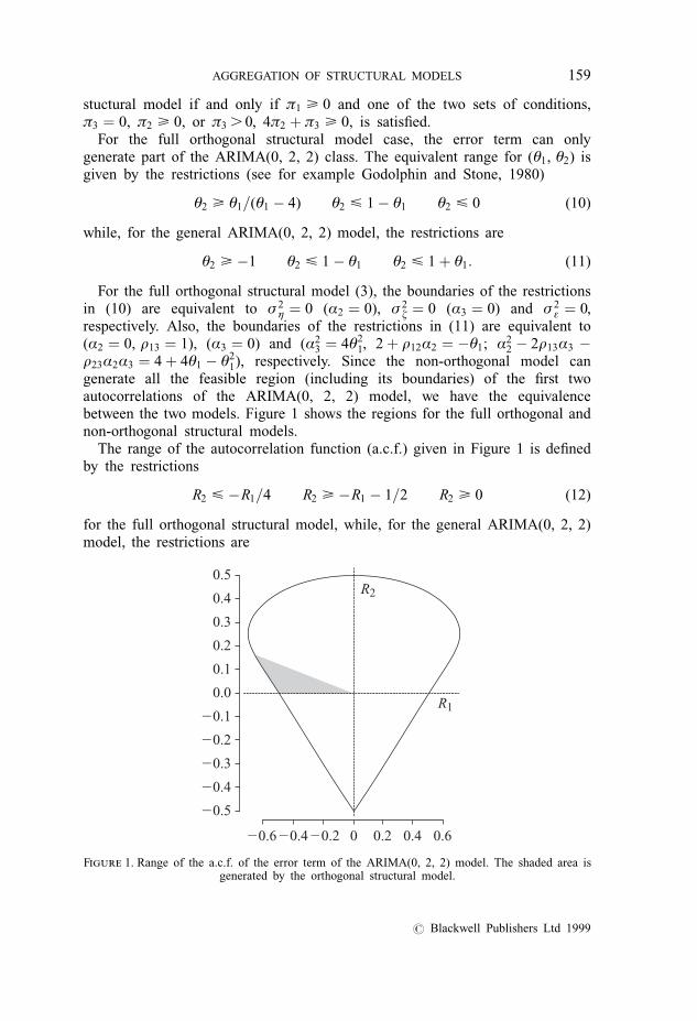
1), respectively. Since the non-orthogonal model cangenerate all the feasible region (including its boundaries) of the ®rst twoautocorrelations of the ARIMA(0, 2, 2) model, we have the equivalencebetween the two models. Figure 1 shows the regions for the full orthogonal andnon-orthogonal structural models.

The range of the autocorrelation function (a.c.f.) given in Figure 1 is de®nedby the restrictions

R2 < ÿR1=4 R2 > ÿR1 ÿ 1=2 R2 > 0 (12)

for the full orthogonal structural model, while, for the general ARIMA(0, 2, 2)model, the restrictions are

20.620.420.2 0 0.2 0.4 0.6

20.5

20.4

20.3

20.2

20.1

0.0

0.1

0.2

0.3

0.4

0.5R2

R1

Figure 1. Range of the a.c.f. of the error term of the ARIMA(0, 2, 2) model. The shaded area isgenerated by the orthogonal structural model.

AGGREGATION OF STRUCTURAL MODELS 159

# Blackwell Publishers Ltd 1999

R21 � 8R2

2 ÿ 4R2 < 0 R2 > ÿR1 ÿ 1=2 R2 > R1 ÿ 1=2: (13)

Equations (12) and (13) are obtained from (10) and (11), respectively, using therelation between the a.c.f. of the error et de®ned in (7) and è1 and è2.

3. AGGREGATION AND DISAGGREGATION OF STRUCTURAL MODELS

Now consider the aggregate series

Yô � yôm � � � � � yômÿm�1 � (1� B � � � � � Bmÿ1)yôm (14)

where m is the period of aggregation. In this section we assume that thedisaggregate series yt (aggregate series Yô) is generated by an ARIMA orstructural model and we derive the necessary conditions for the aggregate series(disaggregate series) to be represented as an ARIMA or structural model.

3.1. Local level structural model

Applying the method used by Telser (1967), we have from Equations (1) and(14) that the aggregate variable Yô is given by

(1ÿ Bm)Yô � (1� B � � � � � Bmÿ1)2fçôm � (1ÿ B)åômg � Dô (15)

with the autocovariances of the error term Dô being given by

Ã0 � 2m3 � m

3á2 � 2m� 2mrá

� �ó 2å

Ã1 � m3 ÿ m

6á2 ÿ mÿ mrá

� �ó 2å (16)

à j � 0 j > 2

where á � óç=óå. Thus, we can model the aggregate series as an ARIMA(0, 1,1) process of the form

(1ÿ B)Yô � (1ÿÈB)Aô � Dô (17)

where B is such that BYô � Yôÿ1. We have seen that the parameters of theARIMA(0, 1, 1) model given by Equation (2) can be easily related to theparameters of the local level model (1) by equating the autocovariance functions.Using this, we arrive at the ®rst-order autocorrelation of the error term Dô as

R1 � (1� è2)(m2 ÿ 1)ÿ 2è(m2 � 2)

2(1� è2)(2m2 � 1)ÿ 8è(m2 ÿ 1): (18)

From the relationship between ARIMA(0, 1, 1) and local level structuralmodels given in Section 2.1, the aggregate series can be modelled as

160 L. K. HOTTA AND K. L. VASCONCELLOS

# Blackwell Publishers Ltd 1999

Yô � Mô � Eô

Mô � Môÿ1 � ô(19)

where Eô and Hô are white noise processes with variances equal to ó 2E and ó 2

H,respectively, with à � cov(Eô, Hô9) equal to zero when ô 6� ô9 and constantwhen ô � ô9.

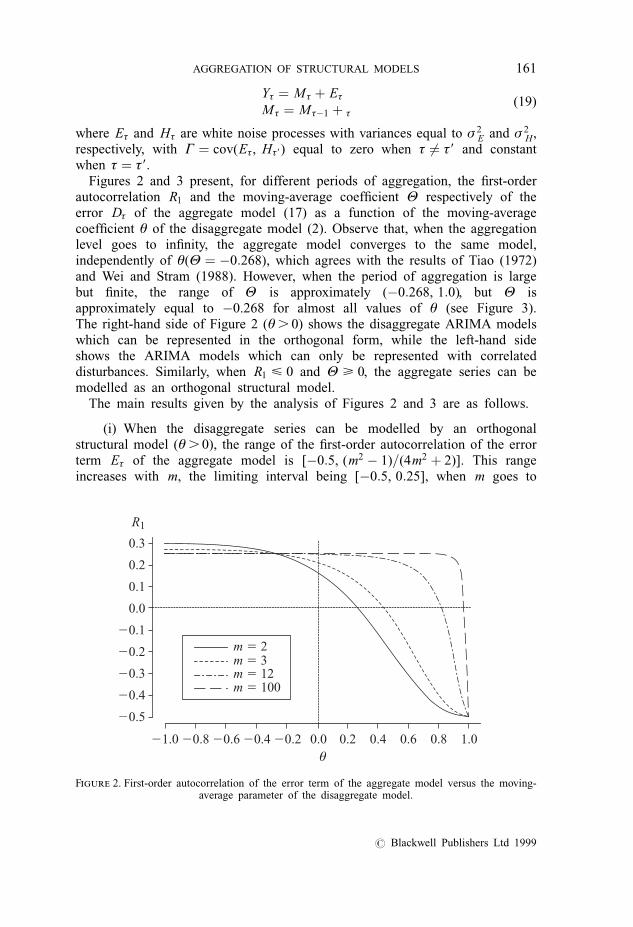
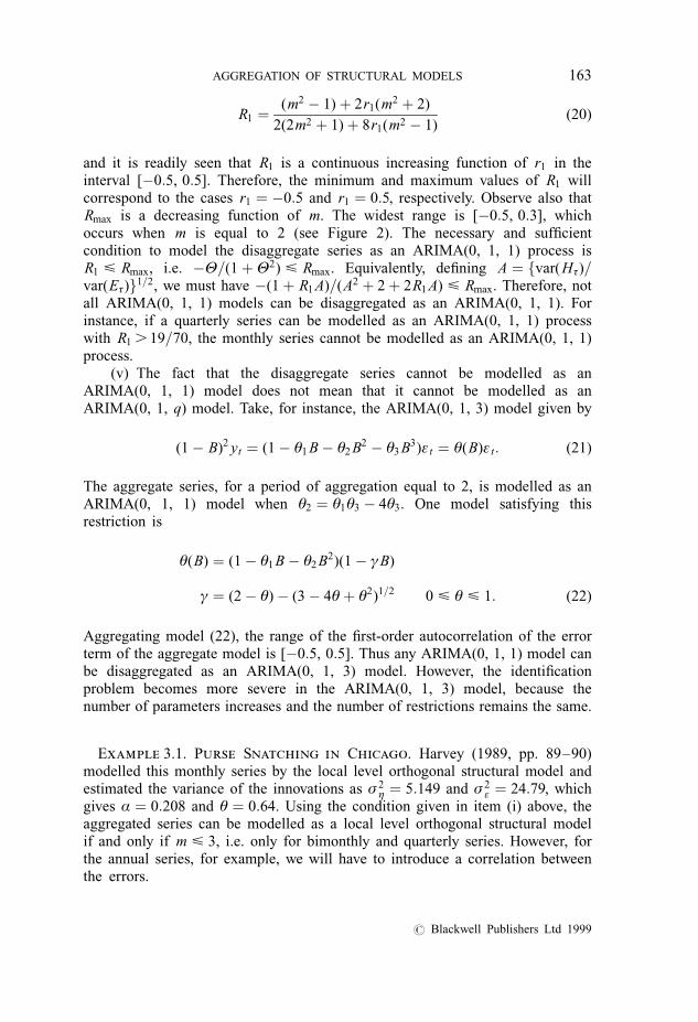
Figures 2 and 3 present, for different periods of aggregation, the ®rst-orderautocorrelation R1 and the moving-average coef®cient È respectively of theerror Dô of the aggregate model (17) as a function of the moving-averagecoef®cient è of the disaggregate model (2). Observe that, when the aggregationlevel goes to in®nity, the aggregate model converges to the same model,independently of è(È � ÿ0:268), which agrees with the results of Tiao (1972)and Wei and Stram (1988). However, when the period of aggregation is largebut ®nite, the range of È is approximately (ÿ0:268, 1:0), but È isapproximately equal to ÿ0.268 for almost all values of è (see Figure 3).The right-hand side of Figure 2 (è. 0) shows the disaggregate ARIMA modelswhich can be represented in the orthogonal form, while the left-hand sideshows the ARIMA models which can only be represented with correlateddisturbances. Similarly, when R1 < 0 and È > 0, the aggregate series can bemodelled as an orthogonal structural model.

The main results given by the analysis of Figures 2 and 3 are as follows.

(i) When the disaggregate series can be modelled by an orthogonalstructural model (è. 0), the range of the ®rst-order autocorrelation of the errorterm Eô of the aggregate model is [ÿ0:5, (m2 ÿ 1)=(4m2 � 2)]. This rangeincreases with m, the limiting interval being [ÿ0:5, 0:25], when m goes to

m 5 2m 5 3m 5 12m 5 100

21.0 20.8 20.6 20.4 20.2 0.0 0.2 0.4 0.6 0.8 1.0θ

20.5

20.4

20.3

20.2

20.1

0.0

0.1

0.2

0.3

R1

Figure 2. First-order autocorrelation of the error term of the aggregate model versus the moving-average parameter of the disaggregate model.

AGGREGATION OF STRUCTURAL MODELS 161

# Blackwell Publishers Ltd 1999

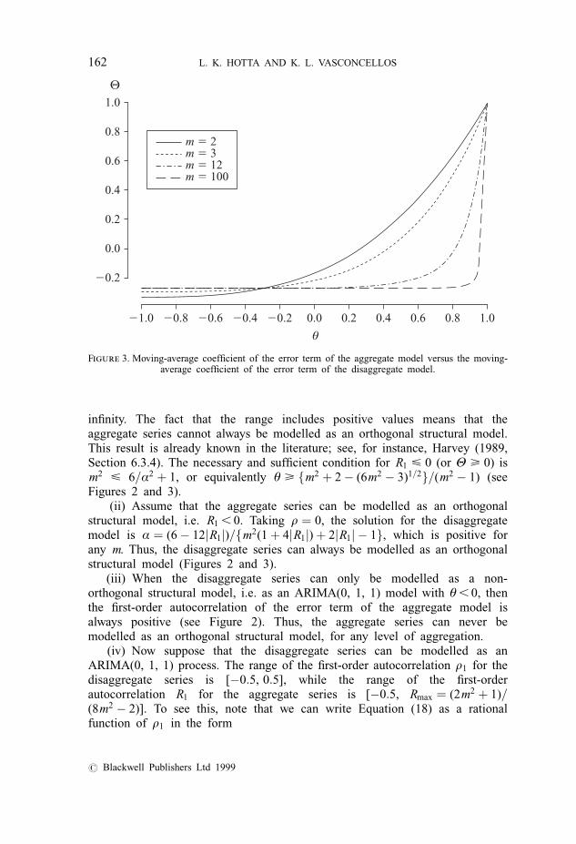
in®nity. The fact that the range includes positive values means that theaggregate series cannot always be modelled as an orthogonal structural model.This result is already known in the literature; see, for instance, Harvey (1989,Section 6.3.4). The necessary and suf®cient condition for R1 < 0 (or È > 0) ism2 < 6=á2 � 1, or equivalently è > fm2 � 2ÿ (6m2 ÿ 3)1=2g=(m2 ÿ 1) (seeFigures 2 and 3).

(ii) Assume that the aggregate series can be modelled as an orthogonalstructural model, i.e. R1 , 0. Taking r � 0, the solution for the disaggregatemodel is á � (6ÿ 12jR1j)=fm2(1� 4jR1j)� 2jR1j ÿ 1g, which is positive forany m. Thus, the disaggregate series can always be modelled as an orthogonalstructural model (Figures 2 and 3).

(iii) When the disaggregate series can only be modelled as a non-orthogonal structural model, i.e. as an ARIMA(0, 1, 1) model with è, 0, thenthe ®rst-order autocorrelation of the error term of the aggregate model isalways positive (see Figure 2). Thus, the aggregate series can never bemodelled as an orthogonal structural model, for any level of aggregation.

(iv) Now suppose that the disaggregate series can be modelled as anARIMA(0, 1, 1) process. The range of the ®rst-order autocorrelation r1 for thedisaggregate series is [ÿ0:5, 0:5], while the range of the ®rst-orderautocorrelation R1 for the aggregate series is [ÿ0:5, Rmax � (2m2 � 1)=(8m2 ÿ 2)]. To see this, note that we can write Equation (18) as a rationalfunction of r1 in the form

m 5 12m 5 3m 5 2

m 5 100

21.0 20.8 20.6 20.4 20.2 0.0 0.2 0.4 0.6 0.8 1.0

θ

20.2

0.0

0.2

0.4

0.6

0.8

1.0

Θ

Figure 3. Moving-average coef®cient of the error term of the aggregate model versus the moving-average coef®cient of the error term of the disaggregate model.

162 L. K. HOTTA AND K. L. VASCONCELLOS

# Blackwell Publishers Ltd 1999

R1 � (m2 ÿ 1)� 2r1(m2 � 2)

2(2m2 � 1)� 8r1(m2 ÿ 1)(20)

and it is readily seen that R1 is a continuous increasing function of r1 in theinterval [ÿ0:5, 0:5]. Therefore, the minimum and maximum values of R1 willcorrespond to the cases r1 � ÿ0:5 and r1 � 0:5, respectively. Observe also thatRmax is a decreasing function of m. The widest range is [ÿ0:5, 0:3], whichoccurs when m is equal to 2 (see Figure 2). The necessary and suf®cientcondition to model the disaggregate series as an ARIMA(0, 1, 1) process isR1 < Rmax, i.e. ÿÈ=(1�È2) < Rmax. Equivalently, de®ning A � fvar(Hô)=var(Eô)g1=2, we must have ÿ(1� R1 A)=(A2 � 2� 2R1 A) < Rmax. Therefore, notall ARIMA(0, 1, 1) models can be disaggregated as an ARIMA(0, 1, 1). Forinstance, if a quarterly series can be modelled as an ARIMA(0, 1, 1) processwith R1 . 19=70, the monthly series cannot be modelled as an ARIMA(0, 1, 1)process.

(v) The fact that the disaggregate series cannot be modelled as anARIMA(0, 1, 1) model does not mean that it cannot be modelled as anARIMA(0, 1, q) model. Take, for instance, the ARIMA(0, 1, 3) model given by

(1ÿ B)2 yt � (1ÿ è1 Bÿ è2 B2 ÿ è3 B3)å t � è(B)å t: (21)

The aggregate series, for a period of aggregation equal to 2, is modelled as anARIMA(0, 1, 1) model when è2 � è1è3 ÿ 4è3. One model satisfying thisrestriction is

è(B) � (1ÿ è1 Bÿ è2 B2)(1ÿ ãB)

ã � (2ÿ è)ÿ (3ÿ 4è� è2)1=2 0 < è < 1: (22)

Aggregating model (22), the range of the ®rst-order autocorrelation of the errorterm of the aggregate model is [ÿ0:5, 0:5]. Thus any ARIMA(0, 1, 1) model canbe disaggregated as an ARIMA(0, 1, 3) model. However, the identi®cationproblem becomes more severe in the ARIMA(0, 1, 3) model, because thenumber of parameters increases and the number of restrictions remains the same.

Example 3.1. Purse Snatching in Chicago. Harvey (1989, pp. 89±90)modelled this monthly series by the local level orthogonal structural model andestimated the variance of the innovations as ó 2

ç � 5:149 and ó 2å � 24:79, which

gives á � 0:208 and è � 0:64. Using the condition given in item (i) above, theaggregated series can be modelled as a local level orthogonal structural modelif and only if m < 3, i.e. only for bimonthly and quarterly series. However, forthe annual series, for example, we will have to introduce a correlation betweenthe errors.

AGGREGATION OF STRUCTURAL MODELS 163

# Blackwell Publishers Ltd 1999

3.2. Local trend structural model

Using Equations (5) and (14), the aggregate variable Yô can be written in theform

(1ÿ Bm)2Yô � (1� B � � � � � Bmÿ1)3fBæôm � (1ÿ B)çôm � (1ÿ B)2åômg � Eô

(23)

with the autocovariances of the error term Eô given by

Ã0 � 6mð1 � m(m2 � 1)ð2 � m(11m4 � 5m2 � 4)

20ð3

Ã1 � ÿ4mð1 ÿ m(m2 � 2)

3ð2 � m(m2 ÿ 1)(13m2 � 8)

60ð3

(24)

Ã2 � mð1 ÿ m(m2 ÿ 1)

6ð2 � m(m2 ÿ 1)(m2 ÿ 4)

120ð3

à j � 0 j > 3

where m is the period of aggregation and ð1, ð2, ð3 are the ð parameters for thedisaggregate series, de®ned in (8). This shows that as expected, the aggregateseries can be represented as an ARIMA(0, 2, 2) process.

From the equations above, we can see that the ð parameters Ð1, Ð2, Ð3 ofthe aggregate series can be written in terms of ð1, ð2, ð3 as

Ð1 � mð1 ÿ m(m2 ÿ 1)

6ð2 � m(m2 ÿ 1)(m2 ÿ 4)

120ð3

Ð2 � m3ð2

m3(m2 ÿ 1)

4ð3 (25)

Ð3 � m5ð3:

From Section 2.2 the aggregate series can be modelled by a full orthogonallocal trend structural model if and only if the two conditions

Ð1 > 0 Ð2 > 0 (26)

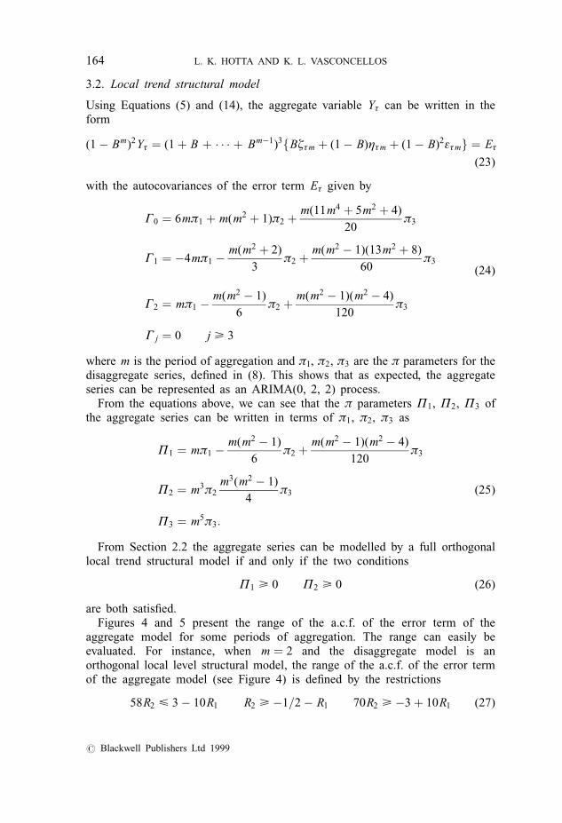
are both satis®ed.Figures 4 and 5 present the range of the a.c.f. of the error term of the

aggregate model for some periods of aggregation. The range can easily beevaluated. For instance, when m � 2 and the disaggregate model is anorthogonal local level structural model, the range of the a.c.f. of the error termof the aggregate model (see Figure 4) is de®ned by the restrictions

58R2 < 3ÿ 10R1 R2 > ÿ1=2ÿ R1 70R2 > ÿ3� 10R1 (27)

164 L. K. HOTTA AND K. L. VASCONCELLOS

# Blackwell Publishers Ltd 1999

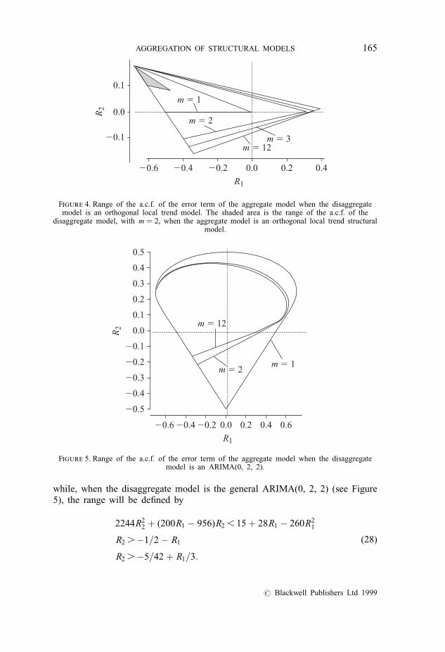
while, when the disaggregate model is the general ARIMA(0, 2, 2) (see Figure5), the range will be de®ned by

2244R22 � (200R1 ÿ 956)R2 , 15� 28R1 ÿ 260R2

1

R2 .ÿ1=2ÿ R1

R2 .ÿ5=42� R1=3:

(28)

m 5 1

m 5 2

m 5 3m 5 12

20.6 20.4 20.2 0.0 0.2 0.4

R1

20.1

0.0

0.1

R2

Figure 4. Range of the a.c.f. of the error term of the aggregate model when the disaggregatemodel is an orthogonal local trend model. The shaded area is the range of the a.c.f. of the

disaggregate model, with m � 2, when the aggregate model is an orthogonal local trend structuralmodel.

m 5 1m 5 2

m 5 12

20.6 20.4 20.2 0.0 0.2 0.4 0.6

R1

20.5

20.4

20.3

20.2

20.1

0.0

0.1

0.2

0.3

0.4

0.5

R2

Figure 5. Range of the a.c.f. of the error term of the aggregate model when the disaggregatemodel is an ARIMA(0, 2, 2).

AGGREGATION OF STRUCTURAL MODELS 165

# Blackwell Publishers Ltd 1999

The main results for the local trend structural model are as follows.

(i) Some orthogonal local trend structural models cannot be aggregated asthe same class of model (see Figure 4). In fact, the aggregation of a fullorthogonal structural model will not generally lead to a full orthogonalstructural model if one of the two positivity conditions in (26), is not satis®ed.For example, for m equal to 2, the aggregate series will be modelled as a fullorthogonal structural model only if the a.c.f. of the error term of thedisaggregate series is in the shaded area in Figure 4. This region will shrinkconsiderably as m increases, similarly to the local level case.

(ii) Moreover, it can be shown that, if the disaggregate series is modelledby a classical local trend structural model, then the aggregate series will alsobe modelled in this same form if and only if the ®rst condition in (26), namelyÐ1 > 0, is satis®ed.

(iii) Not all ARIMA(0, 2, 2) processes can be disaggregated as anARIMA(0, 2, 2) process (see Figure 5).

(iv) Although not represented in Figures 4 and 5, the results for m . 12 arealmost the same as the result for m � 12. For large but ®xed m, the range ofthe a.c.f. is large. However, for most cases, independently of the disaggregatemodel, the ®rst autocorrelations of the aggregate model error term areapproximately (R1, R2) � (0:3939, 0:01515) (this result can also be found inTiao, 1972). This point is the right vertex of the triangle in Figure 4((è1, è2) � (0, 0) in the disaggregate model), and it is also the crossing of theellipse and the straight line in Figure 5 ((è1, è2) � (ÿ2, ÿ1)) when m goes toin®nity. For ®nite m, for instance m � 12, these points are equal to (0.3916,0.01458) and (0.3962, 0.01573) (Figures 4 and 5, respectively), which arealready very close to the limit value.

(v) We observe that the local level structural model can be put as a specialcase of the local trend model. In particular, we will have ð3 � 0, ð2 � ó 2

ç,ð1 � ó 2

å . Thus, for classical local trend models, the positivity of the ®rstequation in (25) can be seen as an extension of the positivity condition we havefor the local level.

(vi) For a period of aggregation of two units (m � 2) of the classical localtrend model, the last term of the positivity condition vanishes, due to the factorm2 ÿ 4. This means that, when the disaggregated series is represented by aclassical local trend model, the level m � 2 of aggregation has no sensitivity tothe local trend structure, and the condition for representing the aggregatedseries by a classical orthogonal model is the same for the local level and localtrend models.

(vii) Although not pursued here, similarly to the ARIMA(0, 1, 1) model, itis possible to show that the ARIMA(0, 2, 2) model can always bedisaggregated as an ARIMA(0, 2, q), but sometimes q must be larger than 2.

Example 3.2. UK Quarterly Gas Consumption. Harvey (1989, pp. 95±99) modelled this series using an orthogonal local trend plus cycle model. We

166 L. K. HOTTA AND K. L. VASCONCELLOS

# Blackwell Publishers Ltd 1999

will use only the trend component, with variance estimates given by ó 2ç � 6:42,

ó 2æ � 0:29, ó 2

å � 114. The autocorrelations of the error term of the model forthe observed series, given by Equation (6), are r1 � ÿ0:663 and r2 � 0:164.The equivalent ARIMA(0, 2, 2) parameters are è1 � 1:631 and è2 � ÿ0:673.We can see that these values satisfy Equations (10) and (12), con®rming thatthe model can be written as an orthogonal structural model. The ®rst twoautocorrelations of the error term of the aggregate model are fR1 � ÿ0:651,R2 � 0:154g for m � 2 and fR1 � ÿ0:573, R2 � 0:118g for m � 4, accordingto Equations (16). Since both correlations satisfy (12), we have that thesemestral and annual series can be modelled as orthogonal structural models.

4. AGGREGATION OF SEASONAL AND CYCLICAL COMPONENTS

Assume that the observed series is of the additive form, i.e. is the sum of trend,seasonal, cyclical and irregular components. It is natural to consider what willhappen individually to the components when the series is aggregated. Themodels considered up to now were appropriate for trends. In this section, weconsider the models proposed by Harvey (1989) for the seasonal and cyclicalcomponents.

The seasonal component, as suggested by Harvey (1989, Section 2.3.4), ismodelled as

st �Xsÿ1

j�1

stÿ j � ù t (29)

where the ù t form a white noise process such that ù t is uncorrelated with thepast components stÿ j, j . 0, and s is the seasonal period. It is immediate to seethat the aggregated series is

Sô �Xmÿ1

i�0

sômÿi � ÿXrÿ1

j�1

Sôÿ j � Wô (30)

when mr � s. Thus, the aggregated seasonal component can be modelled withthe same form as for the disaggregated seasonal component. Clearly, when m isa multiple of the seasonal period s, the seasonal component disappears with theaggregation, in the sense that the sum of the seasonal terms will produce a whitenoise process which will be added to the observational error. Although the errorvariances are not identi®able anymore, this does not pose a problem since, inpractice, we will not be interested in estimates of the individual variances.

For the cyclical component, Harvey (1989, p. 46) suggested the model

(1ÿ 2r cos ëc B� r2 B2)yt � (1ÿ r cos ëc B)å1 t � r sin ëc Bå2 t

� (1ÿ èB)å t � at (31)

AGGREGATION OF STRUCTURAL MODELS 167

# Blackwell Publishers Ltd 1999

where, in general, å1 t and å2 t are independent white noises with equal variances(see Harvey, 1989, p. 46), 0 ,r, 1 and 0 , ëc ,ð. The autoregressivepolynomial has a pair of complex roots equal to rÿ1 exp(�iëc), which areresponsible for the cyclical behaviour of the series. Thus, the cycle component isan ARMA(2, 1) with autoregressive complex roots and moving-average para-meter equal to

è1� r2

2r cos ëc

� 1� r2

2r cos ëc

!2

ÿ1

8<:9=;

1=2

(32)

with subtraction when 0 , ë,ð=2 and addition for ð=2 , ë,ð.The aggregated series is an ARMA(2, 2) process with autoregressive roots

equal to rÿm exp(�imëc) (see, for instance, Pino et al., 1987).For m � 2 the aggregate model is given by

f1ÿ 2r2 cos(2ëc)r4 L2gYô

� (1� 2r cos ëc B� r2 B2)(1ÿ èB)(1� B)å t � Aô (33)

where L � B2, such that LYô � Yôÿ1. Thus, although the aggregate series stillhas a cyclical behaviour due to the pair of complex roots, it is not the type ofmodel described by (31) anymore, because the moving-average parameter doesnot obey Equation (32), with the appropriate change of r to r2 and of ëc to 2ëc.One could try to decompose the aggregated cycle into two independentcomponents: a cycle of the class of model (31) plus an independent white noisecomponent E2ô. This sum is given by

f1ÿ 2r2 cos(2ëc) L� r4 L2gYô � (1ÿÈL)E1ô

� f1ÿ 2r2 cos(2ëc) L� r4 L2gE2ô � Aô (34)

where È follows a restriction similar to (32). We can see thatE(AôAôÿ2) � r4 var(E2ô), which is always positive, while, in model (34), wehave E(AôAôÿ2) � ÿèr2 var(å t), which is negative for 0 , ëc ,ð=2. Even whenëc .ð=2, equating the ®rst- and second-order autocorrelations of the moving-average terms of models (33) and (34) will result in an incompatible system ofequations, showing that the decomposition is not possible.

Since the aggregation of model (31) will never result in another model of thesame class, we have that model (31) cannot be disaggregated into anothermodel of the same class.

For m . 2, it can be shown that the aggregated process can still have a cyclecomponent representation if the parameters satisfy some equality constraints.For instance, for m � 3 and ëc ,ð=4, we have a single equality constraint,which is

168 L. K. HOTTA AND K. L. VASCONCELLOS

# Blackwell Publishers Ltd 1999

r � cos ëc

cos(2ëc)ÿ cos ëc

cos(2ëc)

� �2

ÿ1

" #1=2

: (35)

However, in practice it is very dif®cult for the process to satisfy these equalityconstraints exactly, which means that the aggregate process will still, in general,be a non-reducible ARMA(2, 2) in the form speci®ed by Pino et al.

5. SYSTEMATIC SAMPLING

We now study the case when a process that satis®es a given model is observedonly at speci®c instants of time, which are multiples of a basic observing periodof length l. This means that we study the process uh de®ned by

uh � yhl h � 1, 2, . . .: (36)

Suppose that the original process fytg can be modelled by an ARIMA(0, d,d) structure. From Brewer (1973), it can readily be seen that the process uh

will also follow an ARIMA(0, d, d) model. A similar result will hold for thelocal level model de®ne in Section 2.1. For this case, it can be seen that if yt

follows the simple orthogonal local level structural model then uh will bemodelled as

uh � mh � vh

mh � mhÿ1 � wh

(37)

where vh and wh are white noise processes with variances given, respectively, byó 2å and ló 2

ç. Therefore. in this case, systematic sampling still yields a process inthe same class of orthogonal structural models as the original process. The sameis not true for a higher order orthogonal model. Suppose now that yt follows theorthogonal local trend structural model introduced in Section 2.2. It is notdif®cult to relate the components ì t and â6 of the state vector to the samecomponents at time t ÿ l. We will obtain the following relations:

ì t � ì tÿ l � lâ tÿ l � v t

â t � â tÿ l � î t

(38)

where v t and î t can be expressed in terms of çt and æ t. Thus, we can deducethat the process uh, as de®ned before can be represented as a local trend modelin the form

uh � mh � vh

mh � mhÿ1 � bhÿ1 � w(1)h (39)

bh � hhÿ1 � w(2)h

AGGREGATION OF STRUCTURAL MODELS 169

# Blackwell Publishers Ltd 1999

where w(1)h and w

(2)h will now be white noise processes. From the expressions for

v t and î t in terms of ç t and æ t, we can obtain cov(w(1)h , w

(2)h ) � l2(l ÿ 1)ó 2

æ=2and var(w

(2)h ) � l3ó 2

æ, where ó 2æ is the variance of æ t. Therefore, unless the trend

in the original model is non-stochastic, we will not be able to produce arepresentation of uh in terms of an orthogonal local trend structural model. Thisshows that the process generated by systematic sampling cannot always berepresented by the same state space modelling as the original process.

6. CONCLUDING REMARKS

In this paper we analysed the classes of ARIMA(0, k, k) models, k � 1, 2,orthogonal structural local and trend models and the aggregation/disaggregationproblem. It was shown that even when the disaggregate model can be modelledas a structural model with uncorrelated disturbances, there are situations whenthe aggregate model cannot be modelled with uncorrelated disturbances.However, when the aggregate series can be represented as an orthogonalstructural model, the disaggregate series can also be represented by anorthogonal structural model. For general k, when the observed series ismodelled as an ARIMA(0, k, k) model, the aggregate series will also be anARIMA(0, k, k) model, but the disaggregate series will not always be of thesame type. For those cases, we can only model the disaggregated series asARIMA(0, k, q), for some q . k.

The aggregation of the Harvey cycle model (1989, p. 46) will also result in acomponent of cyclical behaviour, due the the presence of a pair of complexroots in the autoregressive polynomial. However, since in general the aggregateseries will not have the same cyclical behaviour, the disaggregation/aggregationmust be considered carefully when modelling the cycle.

The systematic sampling of a series which obeys a given structure does notnecessarily produce a series that can be modelled by the same particularstructure. We have shown that this is true for the special example of anorthogonal local trend structural model.

ACKNOWLEDGEMENTS

We wish to thank Professor Andrew Harvey and the referee for helpfulcomments. We are also grateful for grants from CNPq and FINEP.

REFERENCES

Brewer, K. R. W. (1973) Some consequences of temporal aggregation and systematic samplingfor ARIMA and ARMAX models. J. Economet. 2, 133±54.

Godolphin, E. and Stone, M. (1980) On the structural representation for polynomial predictor

170 L. K. HOTTA AND K. L. VASCONCELLOS

# Blackwell Publishers Ltd 1999

models. J. R. Stat. Soc. B 42, 35±45.Gonzalez, P. (1992) Temporal aggregation and systematic sampling in structural time-series

models, J. Forecasting 11, 271±81.б (1993) Efectos de la aggregacioÂn temporal y el muestreo sistemaÂtico en modelos estaciones de

series temporales. Rev. Esp. Econ. 10, 111±34.Guerrero, V. M. (1990) Temporal disaggregation of time series: an ARIMA based approach. In.

Stat. Rev. 58, 29±46.Harvey, A. C. (1989) Forecasting, Structural Time Series Models and the Kalman Filter,

Cambridge: Cambridge University Press.б and Stock, J. H. (1994) Estimation, smoothing, interpolation, and distribution for structural

time-series models in continuous time. In Models, Methods and Applications of Econometrics(ed P. C. Phillips). Oxford: Basil Blackwell, pp. 55±70.

Nijman, T. E. and Palm, F. C. (1990) Predictive accuracy gain from disaggregate sampling inARIMA models. J. Bus. Econ. Stat. 8, 405±15.

Pino, F. A., Morettin, P. A. and Mentz, R. P. (1987) Modelling and forecasting linearcombination of time series. Int. Stat. Rev. 55, 295±313.

Stram, D. O. and Wei, W. W. S. (1986a) Temporal aggregation in the ARIMA processes. J. TimeSer. Anal. 7, 179±292.

б and б (1996b) A methodological note on the dissaggregation of time series models. J. TimeSer. Anal. 7, 293±302.

Telser, L. G. (1967) Discrete samples and moving sums in stationary stochastic process. J. Amer.Statist. Ass. 62, 484±99.

Tiao, G. C. (1972) Asymptotic behaviour of time series aggregates. Biometrika 59, 525±31.б and Hillmer, S. C. (1978) Some considerations on decomposition of a time series.

Biometrika, 65, 497±502.Vasconcellos, K. L. P. (1992) Aspects of forecasting aggregate and discrete data. Unpublished

Ph.D. Dissertation, University of Warwick.Wei, W. W. S. and Stram, D. O. (1988) An eigenvalue approach to the limiting behaviour of time

series aggregates. Ann. Inst. Stat. Math. 40, 101±10.West, M. and Harrison, P. J. (1989) Bayesian Forecasting and Dynamic Models. New York:

Springer.

AGGREGATION OF STRUCTURAL MODELS 171

# Blackwell Publishers Ltd 1999