Aerodynamics Final Project

American Institute of Aeronautics and Astronautics

1

Aerodynamics Final Project

James Einwaechter NC State University, Raleigh, NC, 27607, USA

Nomenclature

𝑐 = chord 𝐶 = lift coefficient 𝐶 = pressure coefficient 𝐶 = pressure coefficient for lower surface 𝐶 = pressure coefficient for upper surface x = x-location y = y-location 𝑥 = the x coordinate of the origin 𝑦 = the y coordinate of the origin u = the (i) component of the velocity 𝑈 = freestream velocity v = the (j) component of velocity V = velocity magnitude

I. Abstract HIS project served to plot streamlines superimposed with velocity contour plots, lift coefficient distributions, and pressure coefficient distributions for two objects of interest using MATLAB to apply the Hess Smith Panel

Method. The two airfoils examined in this report are NACA 2412 and NACA 2418. The program code in MATLAB can be easily adjusted for the free-stream velocity and the angles of attack.

II. Procedure Bellanca 8KCAB Decathlon

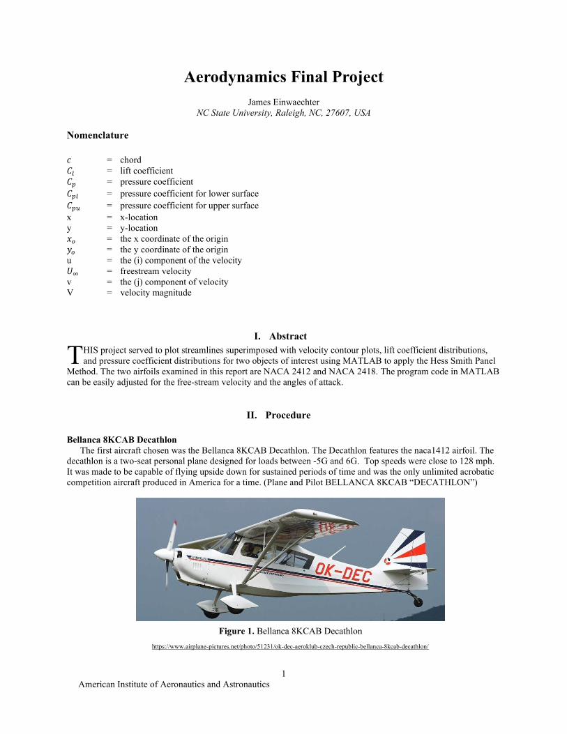
The first aircraft chosen was the Bellanca 8KCAB Decathlon. The Decathlon features the naca1412 airfoil. The decathlon is a two-seat personal plane designed for loads between -5G and 6G. Top speeds were close to 128 mph. It was made to be capable of flying upside down for sustained periods of time and was the only unlimited acrobatic competition aircraft produced in America for a time. (Plane and Pilot BELLANCA 8KCAB “DECATHLON”)

https://www.airplane-pictures.net/photo/51231/ok-dec-aeroklub-czech-republic-bellanca-8kcab-decathlon/

T

Figure 1. Bellanca 8KCAB Decathlon


2

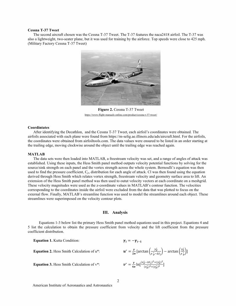
Cessna T-37 Tweet The second aircraft chosen was the Cessna T-37 Tweet. The T-37 features the naca2418 airfoil. The T-37 was

also a lightweight, two-seater plane, but it was used for training by the airforce. Top speeds were close to 425 mph. (Military Factory Cessna T-37 Tweet)

https://www.flight-manuals-online.com/product/cessna-t-37-tweet/

Coordintates

After identifying the Decathlon, and the Cessna T-37 Tweet, each airfoil’s coordinates were obtained. The airfoils associated with each plane were found from https://m-selig.ae.illinois.edu/ads/aircraft.html. For the airfoils, the coordinates were obtained from airfoiltools.com. The data values were ensured to be listed in an order starting at the trailing edge, moving clockwise around the object until the trailing edge was reached again. MATLAB

The data sets were then loaded into MATLAB, a freestream velocity was set, and a range of angles of attack was established. Using these inputs, the Hess Smith panel method outputs velocity potential functions by solving for the source/sink strength on each panel and the vortex strength across the whole system. Bernoulli’s equation was then used to find the pressure coefficient, Cp, distribution for each angle of attack. Cl was then found using the equation derived through Hess Smith which relates vortex strength, freestream velocity and geometry surface area to lift. An extension of the Hess Smith panel method was then used to outut velocity vectors at each coordinate on a meshgrid. These velocity magnitudes were used as the z-coordinate values in MATLAB’s contour function. The velocities corresponding to the coordinates inside the airfoil were excluded from the data that was plotted to focus on the external flow. Finally, MATLAB’s streamline function was used to model the streamlines around each object. These streamlines were superimposed on the velocity contour plots.

III. Analysis Equations 1-3 below list the primary Hess Smith panel method equations used in this project. Equations 4 and

5 list the calculation to obtain the pressure coefficient from velocity and the lift coefficient from the pressure coefficient distribution.

Equation 1. Kutta Condition: 𝜸𝒊 = −𝜸𝒊 𝟏

Equation 2. Hess Smith Calculation of u*: 𝒖∗ =𝜸

𝟐𝝅[arctan

∗

∗ ∆− arctan

∗

∗]

Equation 3. Hess Smith Calculation of v*: 𝒗∗ =𝜸

𝟒𝝅ln[

( ∗ ∆ ) ( ∗ )

( ∗ ) ( ∗ )]

Figure 2. Cessna T-37 Tweet


3

Equation 4. Bernoulli Equation for Cp: 𝑪𝒑 = 𝟏 −𝑽𝟐

𝑼 𝟐

Equation 5. Cl calculation from source strengths: 𝑪𝒍 = 𝟐 ∗ ∗ ∑ ∆𝑆

A. Lift and Pressure Coefficient Distributions

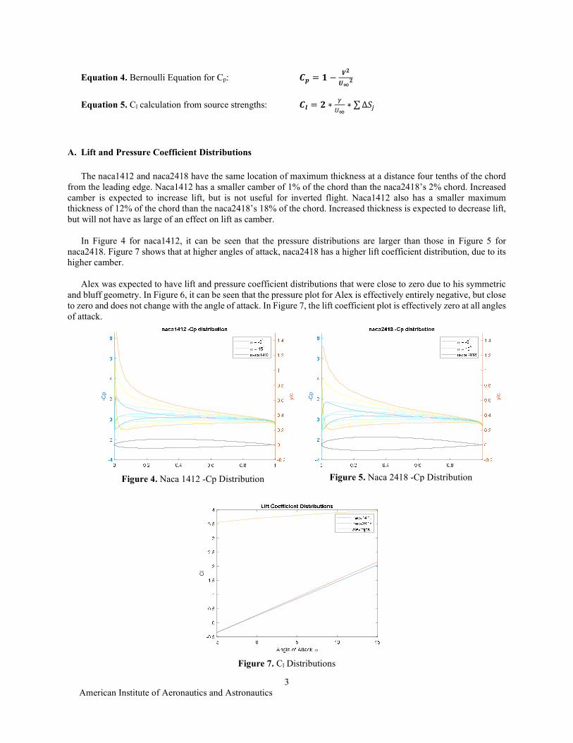
The naca1412 and naca2418 have the same location of maximum thickness at a distance four tenths of the chord from the leading edge. Naca1412 has a smaller camber of 1% of the chord than the naca2418’s 2% chord. Increased camber is expected to increase lift, but is not useful for inverted flight. Naca1412 also has a smaller maximum thickness of 12% of the chord than the naca2418’s 18% of the chord. Increased thickness is expected to decrease lift, but will not have as large of an effect on lift as camber. In Figure 4 for naca1412, it can be seen that the pressure distributions are larger than those in Figure 5 for naca2418. Figure 7 shows that at higher angles of attack, naca2418 has a higher lift coefficient distribution, due to its higher camber. Alex was expected to have lift and pressure coefficient distributions that were close to zero due to his symmetric and bluff geometry. In Figure 6, it can be seen that the pressure plot for Alex is effectively entirely negative, but close to zero and does not change with the angle of attack. In Figure 7, the lift coefficient plot is effectively zero at all angles of attack.

-Cp

y/c

-Cp

y/c

Cl

Figure 4. Naca 1412 -Cp Distribution Figure 5. Naca 2418 -Cp Distribution

Figure 7. Cl Distributions


4

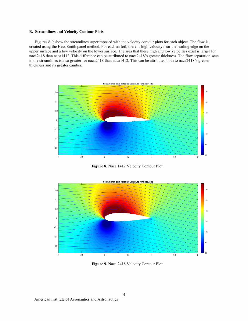
B. Streamlines and Velocity Contour Plots Figures 8-9 show the streamlines superimposed with the velocity contour plots for each object. The flow is

created using the Hess Smith panel method. For each airfoil, there is high velocity near the leading edge on the upper surface and a low velocity on the lower surface. The area that these high and low velocities exist is larger for naca2418 than naca1412. This difference can be attributed to naca2418’s greater thickness. The flow separation seen in the streamlines is also greater for naca2418 than naca1412. This can be attributed both to naca2418’s greater thickness and its greater camber.

Figure 8. Naca 1412 Velocity Contour Plot

Figure 9. Naca 2418 Velocity Contour Plot


5

IV. Conclusion This project highlighted the aerodynamic differences between two airfoils. The Decathlon’s airfoil was observed

to have a smaller camber and maximum thickness in its airfoil than the T-37 Tweet. As a result, the Decathlon had a smaller lift at high angles of attack. This was expected because the goal of this aircraft was to have high aerobatic performance and be able to experience inverted flight for sustained periods of time. The T-37 Tweet was used as a trainer plane for the Air Force, so it needed to be designed for higher speeds. These differences can be visualized in the velocity contour plots where naca 2418 causes more of the flow to speed up on its upper surface and more of the flow to slow down on its lower surface than naca1412.


6

Appendix

MATLAB Code % Aerodynamics Project 2 % James Einwaechter % 5/6/2019 clear close all clc for k = 1:3 airfoils = ["naca1412","naca2418","alexrojas"]; coords = flip(load(sprintf('%s.txt',airfoils(k))),1); x=coords(:,1); y=coords(:,2); uinf = 120; %(free-stream velocity) alphas = -5:5:15; %(angle of attack; degrees) npanel = length(x)-1; cc = jet(length(alphas)); % used to color Cp lines figure() for l = 1:length(alphas) alpha=alphas(l)*pi/180.0; for j=1:npanel ds(j) = sqrt((x(j+1)-x(j)).^2 + (y(j+1)-y(j)).^2); % panel length tnx(j) = (x(j+1)-x(j))./ds(j); % x component of panel tangent = cos(theta_j) tny(j) = (y(j+1)-y(j))./ds(j); % y component of panel tangent = sin(theta_j) xnx(j) = -tny(j); % x component of panel normal xny(j) = tnx(j); % y component of panel normal end %apply V dot n = 0.0 for every panel for i=1:npanel xi = 0.5*(x(i)+x(i+1)); yi = 0.5*(y(i)+y(i+1)); sumn = 0.0; sumt = 0.0; for j=1:npanel xj = x(j); yj = y(j); xip = tnx(j).*(xi-xj) + tny(j).*(yi-yj); %x* location in panel coord. system yip = -tny(j).*(xi-xj) + tnx(j).*(yi-yj); %y* location in panel coord. system upv = 0.5/pi.*(atan2(yip,xip-ds(j))-atan2(yip,xip)); %x* velocity in panel coord. system. vpv = 0.25/pi.*log(((xip-ds(j)).^2 + yip.^2)/(xip.^2 + yip.^2)); %y* velocity in panel coord. system if (i==j) upv = 0.5; vpv = 0.0;


7

end uv = tnx(j).*upv - tny(j).*vpv; %x component of induced velocity in Cart. system vv = tny(j).*upv + tnx(j).*vpv; %y component of induced velocity in Cart. system us = -vv; %x component of source velocity vs = uv; %y component of source velocity a(i,j) = us.*xnx(i) + vs.*xny(i); %matrix elements at(i,j) = us.*tnx(i) + vs.*tny(i); %matrix elements storing tangential components sumn = sumn + uv.*xnx(i) + vv.*xny(i); sumt = sumt + uv.*tnx(i) + vv.*tny(i); end a(i,npanel+1) = sumn; b(i) = -uinf.*(cos(alpha).*xnx(i) + sin(alpha).*xny(i)); at(i,npanel+1) = sumt; end % --- apply Kutta condition for j=1:npanel+1 a(npanel+1,j) = at(1,j)+at(npanel,j); end b(npanel+1) = -uinf.*(cos(alpha).*(tnx(1)+tnx(npanel)) + sin(alpha).*(tny(1)+tny(npanel))); % ----now solve A*ss = b to get the source strengths (ss(1:npanel)) and vortex strength (ss(npanel+1)) % Note that your matrix is (npanel+1,npanel+1) ss = linsolve(a,b')'; % ---- now compute tangential velocity and cp for each panel for i=1:npanel xi(i) = 0.5.*(x(i)+x(i+1)); yi = 0.5.*(y(i)+y(i+1)); sums = 0.0; for j=1:npanel+1 sums = sums + at(i,j).*ss(j); end vtan = sums + uinf.*(cos(alpha).*tnx(i) + sin(alpha).*tny(i)); cp(i) = 1.0 - vtan.^2/uinf.^2; %Cp end hold on yyaxis left txt = sprintf('\\alpha = %d^\\circ', round(alpha*180/pi,0)); cplines(l)=plot(xi,-cp,'-','color', cc(l, :),'DisplayName',txt); xlim([0,1]); ylabel('-Cp'); if k==3 ylim([-6,6.5]); else ylim([-4,8.5]); end cl(l,k) = 2*ss(j)*sum(ds)./uinf; end legend(cplines([1,end])) %plot cp


8

yyaxis right airfoil = plot(x,y,'k','DisplayName',sprintf('%s',airfoils(k))); legend show ylim([-.2, 1.5]); ylabel('y/c');xlabel('x/c'); title(sprintf('%s -Cp distribution',airfoils(k))); hold off if k==3 %plot cl figure() plot(alphas,cl); ylabel('Cl');xlabel('Angle of Attack \alpha'); title('Lift Coefficient Distributions') legend(airfoils); end alpha=alphas(1)*pi/180.0; ifield=500; jfield = 500; [xfield,yfield] = meshgrid(linspace(-1,2,500),linspace(-.75,.75,500)); for jj=1:jfield % loop over field points - for ii=1:ifield xi = xfield(ii,jj); yi = yfield(ii,jj); dksq = sqrt((xi-x).^2+(yi-y).^2); % take out the inside of the object [I,J]=min(dksq); dotp=dot([xnx(J),xny(J)],[x(J)-xi,y(J)-yi]); if k==3 && dotp<0 && min(x)<=xi && xi<=max(x)&& min(y)<= yi&& yi<=max(y) xi=NaN; yi=NaN; elseif k~=3 && dotp>0 && min(x)<=xi && xi<=max(x)&& min(y)<= yi&& yi<=max(y) xi=NaN; yi=NaN; end ufield(ii,jj) = 0.0; % initializes field velocity data vfield(ii,jj) = 0.0; for j=1:npanel xj = x(j); yj = y(j); xip = tnx(j)*(xi-xj) + tny(j)*(yi-yj); yip = -tny(j)*(xi-xj) + tnx(j)*(yi-yj); upv = 0.5/pi*(atan2(yip,xip-ds(j))-atan2(yip,xip)); vpv = 0.25/pi*log(((xip-ds(j)).^2 + yip.^2)./(xip.^2 + yip.^2)); if(x(j)==xi) && (y(j)==yi) upv = 0.5; vpv = 0.0; end if(x(j+1)==xi) && (y(j+1)==yi) upv = 0.0; vpv = 0.5; end uv = tnx(j)*upv - tny(j)*vpv;


9

vv = tny(j)*upv + tnx(j)*vpv; us = -vv; vs = uv; ufield(ii,jj) = ufield(ii,jj) + us*ss(j) + uv*ss(npanel+1); % superimposes velocities for sources and vortex vfield(ii,jj) = vfield(ii,jj) + vs*ss(j) + vv*ss(npanel+1); % superimposes velocities for sources and vortex end ufield(ii,jj) = ufield(ii,jj) + uinf*cos(alpha); % add free stream vfield(ii,jj) = vfield(ii,jj) + uinf*sin(alpha); % add free stream vmag(ii,jj) = sqrt(ufield(ii,jj)^2+vfield(ii,jj)^2); end end figure() starty = -.75:0.05:.75; %define where to start streamlines startx = -ones(size(starty)); [~,h] = contourf(xfield,yfield, vmag,300); hold on h.LineColor = 'none'; colorbar caxis([uinf*.5,uinf*1.6]); %scale contour as function of freestream pbaspect([2 1 1]); colormap jet title(sprintf('Streamlines and Velocity Contours for %s',airfoils(k))); %streamline(xfield,yfield,ufield, vfield,startx,starty) streamslice(xfield,yfield,ufield, vfield,'noarrows'); hold off clearvars -except cl end

Works Cited Military Factory Cessna T-37 Tweet. 2019. Web Publication. 5 May 2019. Plane and Pilot BELLANCA 8KCAB “DECATHLON”. 28 January 2016. web publication. 5 May 2019.

Documents

Aerodynamics Final Project