Embed Size (px)
Citation preview

HAL Id: tel-01871074https://tel.archives-ouvertes.fr/tel-01871074v3
Submitted on 11 Apr 2019
HAL is a multi-disciplinary open accessarchive for the deposit and dissemination of sci-entific research documents, whether they are pub-lished or not. The documents may come fromteaching and research institutions in France orabroad, or from public or private research centers.
L’archive ouverte pluridisciplinaire HAL, estdestinée au dépôt et à la diffusion de documentsscientifiques de niveau recherche, publiés ou non,émanant des établissements d’enseignement et derecherche français ou étrangers, des laboratoirespublics ou privés.
Advanced polyhedral discretization methods forporomechanical modelling
Michele Botti
To cite this version:Michele Botti. Advanced polyhedral discretization methods for poromechanical modelling. Gen-eral Mathematics [math.GM]. Université Montpellier, 2018. English. NNT : 2018MONTS041. tel-01871074v3

THÈSE POUR OBTENIR LE GRADE DE DOCTEUR
DE L’UNIVERSITE DE MONTPELLIER
En Mathématiques et Modélisation
École doctorale : Information, Structures, Systèmes
Unité de recherche : Institut Montpelliérain Alexander Grothendieck
Advanced polyhedral discretization methods forporomechanical modelling
Présentée par Michele BOTTI
Le 27 Novembre 2018
Sous la direction de Daniele DI PIETRO
Devant le jury composé de
BEIRÃO DA VEIGA Lourenço, Professeur des universités, Università di Milano-Bicocca Rapporteur
BOFFI Daniele, Professeur des universités, Università di Pavia Examinateur
DI PIETRO Daniele, Professeur des universités, Université de Montpellier Directeur
GALLOUËT Thierry, Professeur des universités, Institut de Mathématiques de Marseille Rapporteur
SOCHALA Pierre, Ingénieur, BRGM Co-encadrant
VOHRALÍK Martin, Directeur de recherche, INRIA Paris Président du jury


Acknowledgements
Sono profondamente grato a Daniele A. Di Pietro per essere stato un eccezionale direttoredi tesi durante l’intero svolgersi del dottorato. Ammiro la tua passione e dedizione per laricerca e sono onorato di aver lavorato insieme a questa tesi. Ti ringrazio per avermi sempremanifestato fiducia ed avermi incoraggiato durante tutto il percorso. La tua disponibilità e iltuo supporto sono stati di grandissimo aiuto per raggiungere al meglio questo traguardo.
I would like to thank my second supervisor, Pierre Sochala, for welcoming me at BRGMwithin the best conditions. Thank you for your kindness, your listening, your passion and forall the time we have spent together. It has been a great pleasure to work with you.
I would also like to express my sincere gratitude to Lourenço Beirão da Veiga and ThierryGallouët, who have accepted the heavy task of being referees, for the interest they have shownin my work, and their pertinent suggestions. I am also very grateful to Daniele Boffi andMartin Vohralik for having accepted to be members of the PhD committee.
I would like to thank all the members of the SPU research team that I met during the9 months at the BRGM. I am particularly grateful to André Burnol, Farid Smaï, FernandaM.L. Veloso, and Hideo Aochi for the fruitful discussions about poromechanics and reservoirmodelling. I also express my special thanks to Olivier Le Maître for his collaboration in theresults of the last chapter of this manuscript. I really appreciate your great intuitions andclear explanations.
At the IMAG, I would like to thank the researchers and professors with whom I hadthe opportunity to exchange and work with, especially Berardo Ruffini, Michele Bolognesi,Matthieu Alfaro, Philippe Roche and Vanessa Lleras. I am also grateful to the administra-tive staff, including Bernadette Lacan, Geneviève Carrière, and Carmela Madonia for theirefficiency and patience. Many thanks also to the PhD and post-doctoral students met duringthe years in Montpellier, especially Abel, Alexandre, Francesco, Jocelyn, Joubine, Mario,Nestor, Paul, Paul-Marie, Rita, Robert, Rodrigo, and Tiffany. I am also particularly gratefulto Alice, Fatima, Roberta for the good moments we shared in our office. Finally, I would liketo express a huge thank to Florent for being a true friend during these three years, not onlyfor the fantastic time we had while traveling around the world, but also for being close to mewhen I needed it most.
Questi tre anni di dottorato mi hanno permesso di incontrare tante altre persone stupende chedesidero ringraziare perché, a modo loro, hanno fortemente contribuito alla realizzazionedi questa tesi. Ringrazio Florent, Alex, Tim, Paul e Alec per avermi accolto al mio arrivoall’IMAG ed avermi fatto sentire sin da subito a casa. Un ringraziamento speciale va anchea tutti i coinquilini dell’appartamento di Rue Rondelet: Gregoire, Jean-Florent, Claire, Swan
i

ii Acknowledgements
e Pierre-Alexis. Condividere le cene, le serate, i weekend con voi ha riempito di gioia la miaesperienza a Montpellier.
Desidero ringraziare gli amici dello Sborgomeo: Rumi, Stiv, Max, Maffo, Zenk, Andree Susi; che sono sempre al mio fianco. I momenti condivisi con voi li porterò nel cuore.Un grande grazie anche agli Sugarcandy Mountains: Cano, Jaya, Oscar, J, Zenk e Zoia. Iconcerti e le prove insieme sono per me un fondamentale momento di amicizia e divertimento.Sono felice che il nostro progetto musicale continui. Scusandomi con chi non ho menzionato,ringrazio anche tutti coloro che, nonostante la lontananza, mi sono stati vicini manifestandomiil loro affetto e la loro amicizia.
Sarò eternamente riconoscente ai miei genitori per avermi fatto sentire il loro amore anchea centinaia di chilometri di distanza. Vi sono grato per tutto ciò che avete fatto e continuate afare per me, per gli insegnamenti ed i valori che mi avete trasmesso. Grazie mamma per il tuosesto senso capace di sentire quando qualche nuvolone grigio fa capolino nel mio cielo anchequando cerco di nasconderlo. Grazie papà per il tuo cuore immenso e per avermi insegnatola gioia del dare agli altri. Grazie Mamie per esserti sempre preoccupata per me. GrazieStefano per la tua vicinanza, la tua energia e la voglia di passare dei bei momenti insieme.Grazie Lorenzo per tutte le ore trascorse a confrontarci sulle nostre teorie e riflessioni. Sonodavvero felice di condividere con te la passione per la matematica. Ringrazio immensamenteAnna e Martine per il loro supporto e per esserci per celebrare questo importante traguardo.
Concludo ringraziando la persona con cui più di tutte ho condiviso le soddisfazioni ele fatiche di questo dottorato. Grazie Claudia per esserci sempre stata con il tuo preziososostegno e per tutta la bellezza e l’amore che mi hai regalato in questi anni.

iii

iv

Résumé
Dans cette thèse, on s’intéresse à de nouveaux schémas de discrétisation afin de résoudreles équations couplées de la poroélasticité et nous présentons des résultats analytiques etnumériques concernant des problèmes issus de la poromécanique. Nous proposons de ré-soudre ces problèmes en utilisant les méthodes Hybrid High-Order (HHO), une nouvelleclasse de méthodes de discrétisation polyédriques d’ordre arbitraire. Cette thèse a été con-jointement financée par le Bureau de Recherches Géologiques et Minières (BRGM) et leLabEx NUMEV. Le couplage entre l’écoulement souterrain et la déformation géomécaniqueest un sujet de recherche crucial pour les deux institutions de cofinancement.
Contexte et motivations
On prend en considération des matériaux constitués d’un squelette solide et d’un réseau depores, connectés entre eux et permettant le passage d’un fluide interstitiel. Le comportementde ce fluide peut influer sur celui du squelette et réciproquement. De nombreux matériauxprésentent cette caractéristique : les matériaux minéraux comme les sols et les roches,des matériaux organiques comme le bois, les os ou le cerveau et les matériaux industrielscomme certains joints d’étanchéité. Dans cette thèse, l’accent porte sur la modélisationdes sols et des roches. Le milieu poreux est vu comme la superposition de deux milieuxcontinus : le squelette solide déformable et la phase fluide. Le milieu poreux possède unecinématique déterminée par le squelette et les sollicitations considérées peuvent être de typemécanique, hydraulique et thermique. Les sollicitations mécaniques peuvent être causées pardes contraintes imposées, telles que le creusement d’ouvrages, ou bien par des contraintesintrinsèques, telles que la consolidation du sol par gravité. Les sollicitations hydrauliquessont liées à l’écoulement du fluide à travers le milieu, tandis que les sollicitations thermiquespeuvent être dues à la présence de sources de chaleur. Lorsque les trois phénomènes sonttraités de manière couplée, le cadre est celui dit de la thermo-hydro-mécanique. Dans cettethèse, on s’intéresse avant tout au modèle hydro-mécanique saturé obtenu en supposant queles variations de température soient négligeables.
L’intérêt pour les mécanismes couplés de diffusion-déformation était initialement motivépar le problème de la consolidation [2727, 189189], à savoir, le tassement progressif du sol dû àl’extraction des fluides. Aujourd’hui la théorie de la poroélasticité présente un intérêt pourles scientifiques et les ingénieurs en raison de son potentiel d’applications dans la mécaniquedes sols, l’industrie pétrolière, la géomécanique environnementale et la biomécanique. Ensimulation de réservoir, le couplage mécanique-écoulement joue un rôle important pourl’étude des problèmes de compaction et subsidence induits par la mise en production de
v
vi
réservoirs peu consolidés, pour la stabilité des puits, ou encore la fracturation hydraulique.La non prise en compte de ce couplage peut aussi conduire à de mauvaises prédictions dela production. Le couplage poroélastic est par ailleurs crucial pour l’étude des risques liés àl’injection et au stockage du CO2 dans les aquifères salins, comme la fuite du CO2 par le puitsou bien la réactivation mécanique des failles. La surpression entraînée par l’injection peutaussi modifier les contraintes appliquées sur la roche couverture et provoquer une fracturationqui remettrait en cause l’intégrité du stockage.
Dans cette thèse, nous considérons principalement trois problèmes liées à la modélisationde la géomécanique : le problème couplé de Biot linéaire dans le Chapitre 22, le comportementnon-linéaire en mécanique et poromécanique dans les chapitres 33 et 44 et la poroélasticité aveccoefficients aléatoires dans le Chapitre 55. Comme noté dans [6868], de nombreux résultatsexpérimentaux suggèrent que la réponse volumétrique de la roche poreuse au changement dela pression totale est en réalité non-linéaire. Cette non-linéarité est généralement associée à lafermeture/ouverture de fissures ou, dans les roches très poreuses, à l’effondrement progressifdes pores. Les études physiques du comportement mécanique non-linéaire des milieuxporeux [2222, 2828] ont été motivées par la nécessité de quantifier l’effet de la diminution de lapression interstitielle lors de l’épuisement d’un gisement de pétrole ou de gaz sur le volumede la matrice rocheuse.
En simulation numérique, la prise en compte des incertitudes dans les données d’entrée(telles que les constantes physiques, les conditions limites et initiales, le forçage externe etla géométrie) est un problème crucial, en particulier dans l’analyse des risques. L’évaluationdes risques dans les applications de poroélasticité reste un défi majeur pour un large éventaild’applications de gestion des ressources essentielles. Les préoccupations récentes de la pop-ulation concernant la sismicité induite et la contamination des eaux souterraines soulignentla nécessité de quantifier la probabilité d’événements nocifs associés à l’écoulement et à ladéformation de la subsurface. La prédiction des contraintes critiques qui peuvent compro-mettre l’intégrité des roches couvertures et la stabilité des puits dans les réservoirs de stockageprésente un intérêt particulier. La clé de la réussite de l’évaluation des risques dans les appli-cations poroélastiques est la capacité de prédire la probabilité d’événements critiques en sebasant sur une approximation empirique des paramètres matériels et de la variabilité du termesource. La quantification d’incertitude fournit des barres d’erreur numériques qui facilitentla comparaison avec l’observation expérimentale et l’évaluation des modèles physiques. Deplus, elle permet d’identifier les paramètres incertains qui doivent être mesurés avec plus deprécision car ils ont un impact plus significatif sur la solution. Parmi les différentes techniquesconçues pour la propagation et la quantification de l’incertitude dans les modèles numériques,dans cette thèse nous considérons les méthodes spectrales stochastiques. L’idée centrale deces méthodes est la décomposition de quantités aléatoires sur des bases d’approximationappropriées telles que les expansions en Polynômes de Chaos [112112, 137137].
Discrétisation
Ces dernières années, un effort important a été consacré au développement et à l’analysede méthodes numériques capables de traiter des maillages plus généraux que les maillagessimpliciaux ou cartésiens. Dans le contexte de la poroélasticité, cette nécessité est motivée par

vii
la présence des couches géologiques et des fractures dans le milieu poreux. La discrétisationdu domaine peut également inclure des éléments dégénérés (comme dans la région prochedu puits dans la modélisation des réservoirs) et des interfaces non-conformes apparaissantlors de la modélisation de l’érosion et de la formation de failles. Dans le contexte dela mécanique des structures, les méthodes supportant les maillages polyédriques générauxpeuvent être utiles pour plusieurs raisons, notamment l’utilisation de nœuds suspendus pourles problèmes de contact et d’interface et la robustesse par rapport aux distorsions et fractures.De plus, les méthodes polyédriques permettent de simplifier les procédures de raffinement etde déraffinement du maillage utilisées pour l’adaptation.
Dans cette thèse, on s’intéresse à deux familles de méthodes de discrétisation polyé-driques d’ordre arbitraire : les méthodes HHO et Galerkin discontinues (dG). L’utilisationde méthodes d’ordre élevé peut accélérer la convergence en présence de solutions régulières,ou lorsqu’elles sont associées au raffinement local du maillage. De plus, la construction deproblèmes discrets à l’aide des discrétisations HHO et dG est valable en dimension d’espacearbitraire permettant d’envisager une mise en œuvre indépendante de la dimension. Lesdeux méthodes sont non-conformes dans le contexte de formulations primales de problèmeselliptiques, car aucune condition de continuité n’est imposée entre les éléments voisins endG et entre les faces voisines en HHO. Nous nous concentrons sur la méthode HHO pour ladiscrètisation de la mécanique et sur la méthode dG pour la discrétisation de l’écoulement.
Les méthodes HHO, introduites dans [7878] et [7474], reposent sur des formulations primalesde problèmes elliptiques et aboutissent à des systèmes symétriques et définis positifs. Lesinconnues discrètes sont des polynômes du même ordre sur les éléments et les faces. Cesderniéres établissent des connexions inter-éléments aux interfaces et peuvent être utiliséespour imposer des conditions limites essentielles aux faces de bord. Les inconnues de maillesont des variables intermédiaires qui peuvent être éliminées du système global par conden-sation statique, comme détaillé dans le Chapitre 22. La conception des méthodes HHO sefait en deux étapes : (i) tout d’abord, on reconstruit des opérateurs différentiels discrètsbasés sur la résolution de problèmes locaux peu coûteux à l’intérieur de chaque élémentet ensuite, (ii) on introduit une stabilisation qui relie entre elles les inconnues discrètesd’élément et de face. Les définitions des opérateurs de reconstructions différentiels sontbasées sur des contreparties discrètes des intégrations par parties. Même si les problèmeslocaux liés aux opérateurs de reconstruction doivent être résolus, les résultats numériquesde [7474] indiquent que le coût associé devient marginal par rapport au coût de la résolutiondu système global. De plus, les méthodes HHO sont efficaces, car l’utilisation d’inconnuesde face donne des stencils compacts. Les méthodes HHO offrent d’autres avantages, dont lapossibilité d’établir des propriétés de conservation de quantités physiques et la robustesse parrapport à l’hétérogénéité des coefficients. La discrétisation HHO étudiée dans le Chapitre 33s’inspire des travaux récents sur les opérateurs Leray–Lions [6969, 7070], où les auteurs montrentque la méthode est robuste en ce qui concerne les non-linéarités.
Les méthodes dG peuvent être considérées comme des méthodes éléments finis permettantdes discontinuités dans les espaces discrets, ou bien comme des volumes finis dans lesquelsla solution approchée est représentée dans chaque élément du maillage par un polynôme aulieu que par une constante. Permettre à la solution d’être continue par morceaux offre unegrande flexibilité dans la conception du maillage. En plus d’être adaptées aux maillages

viii
généraux y compris non-conformes, les méthodes dG ont l’avantage de pouvoir monter enordre très facilement. Leur principal inconvénient est le grand nombre d’inconnues qu’ellesengendrent, et donc le coût de résolution des systèmes. Une analyse unifiée des méthodes dGpour les problèmes elliptiques peut être trouvée dans [4242] et [7676]. La stratégie fondamentalepour approcher le problème de la diffusion hétérogène (tel que le flux darcéen dans les milieuxporeux) en utilisant les méthodes dG consiste à pénaliser les sauts d’interface en utilisant unepondération dépendante de la moyenne harmonique des composantes normales du tenseur dediffusion. Cette technique permet de pénaliser de façon optimale. De plus, comme indiquédans le chapitres 22 et 44 et dans [7777], la méthode proposée est robuste en ce qui concerne lesvariations spatiales du coefficient de perméabilité, avec des constantes dans les estimationsd’erreur ayant une dépendance faible du rapport d’hétérogénéité.
Structure du manuscrit
Par la suite, nous allons résumer brièvement le contenu du manuscrit en mettant l’accent surles résultats marquants.
Dans le Chapitre 11 nous présentons les modèles de poroélasticité que nous allons con-sidérer successivement. Une fois ceux-ci introduits, nous faisons un inventaire des difficultésliées à leur approximation numérique, avant de présenter un état de l’art documenté nouspermettant de définir les orientations des chapitres suivants.
Dans le Chapitre 22, publié dans SIAM Journal on Scientific Computing (voir [3030]), nousintroduisons un nouvel algorithme pour le problème de Biot, basé sur une discrétisation HHOde la mécanique et une discrétisation dG Symmetric Weighted Interior Penalty (SWIP) duflux. La méthode a plusieurs atouts, notamment la validité en deux et trois dimensions, lastabilité inf-sup, le support des maillages polyédriques généraux et l’utilisation de l’ordred’approximation arbitraire en espace. De plus, le coût de résolution peut être réduit encondensant statiquement un grand sous-ensemble d’inconnues. Notre analyse fournit desestimations de stabilité et d’erreur qui se maintiennent même lorsque le coefficient de stockagespécifique est nul et montre que les constantes dépendent faiblement de l’hétérogénéité ducoefficient de perméabilité. Nous discutons les détails de la mise en œuvre de la méthode etfournissons des tests numériques démontrant ses performances. Enfin, nous montrons que leschéma est localement conservateur sur le maillage primal, une propriété souhaitable pourles praticiens et fondamentale pour les estimations a postériori basées sur des flux équilibrés.
Dans le Chapitre 33, publié dans SIAM Journal on Numerical Analysis (voir [3333]), nousproposons et analysons une nouvelle discrétisation HHO d’une classe de modèles d’élasticité(linéaire et) non-linéaire couramment utilisées en mécanique des solides. La méthode sat-isfait un principe local de travail virtuel à l’intérieur de chaque élément du maillage, avecdes tractions numériques d’interface qui obéissent à la loi d’action et réaction. Une analysecomplète couvrant des lois de comportement mécanique très générales est effectuée. En par-ticulier, nous prouvons l’existence d’une solution discrète et nous identifions une hypothèsede monotonie stricte sur la loi contrainte-déformation qui assure l’unicité. La convergenceaux solutions de régularité minimale est démontrée en utilisant un argument de compacité.Une estimation d’erreur optimale d’ordre hk+1 de la norme d’énergie est alors prouvée dansles conditions supplémentaires de continuité de Lipschitz et de forte monotonie sur la loi de

ix
comportement. Les performances de la méthode sont largement étudiées sur un panel com-plet de tests numériques avec des lois contrainte-déformation correspondant à des matériauxréels.
Dans le Chapitre 44, tiré de [3535], nous construisons et analysons une méthode coupléeHHO-dG pour la poroélasticité non-linéaire. Il y a deux différences principales par rapportà la méthode conçue dans le Chapitre 22 pour la version linéaire du problème. Première-ment, le gradient symétrique discret se situe dans l’espace complet des polynômes à valeurstensorielles, par opposition aux gradients symétriques des polynômes à valeurs vectorielles.Comme montré dans le Chapitre 33, cette modification est nécessaire pour l’analyse de conver-gence en présence de lois de comportement non-linéaires. Deuxièmement, le terme de droitedu problème discret est obtenu en prenant la moyenne en temps de la force de chargement f etde la source de fluide g entre deux pas de temps consécutifs. Cette modification nous permetde prouver la stabilité et l’estimation d’erreur sans aucune hypothèse de régularité supplé-mentaire sur les données. Un autre résultat marquant de ce chapitre est une nouvelle preuvede l’inégalité de Korn discrète, ne nécessitant pas d’hypothèse géométrique particulière surle maillage.
Le Chapitre 55 contient des perspectives sur la solution numérique du problème de Biotavec coefficients poroélastiques aléatoires dans le contexte de la quantification des incer-titudes. Il recueille une partie des travaux en cours réalisés lors du stage au BRGM quis’est déroulé de janvier à septembre 2018. L’incertitude est modélisée par un ensemble finide paramètres avec une distribution de probabilité prescrite. Une attention particulière estaccordée pour assurer que la paramétrisation des coefficients soit physiquement admissible.Nous présentons la formulation faible du système d’équations différentielles stochastiqueset établissons sa bonne position. Nous discutons ensuite de l’approximation du problèmepar des techniques non-intrusives basées sur le développement de solutions sur des bases dePolynômes de Chaos. La procédure de projection spectrale considérée permet de réduirele problème stochastique à un ensemble fini de simulations déterministes paramétriquesdiscrétisées par le schéma HHO-dG du Chapitre 22. Nous étudions numériquement la conver-gence de l’erreur par rapport au niveau de la grille dans l’espace de probabilité. Enfin, nouseffectuons une analyse de sensibilité pour évaluer la propagation de l’incertitude en entréesur les champs de déplacement et pression dans un cas test d’injection et un problème detraction.
En Annexe AA, publié dans les actes de la conférence Finite Volumes for Complex Appli-
cations VIII (voir [3434]), nous présentons une variante du schéma HHO-dG pour le problèmede la poroélasticité non-linéaire étudié dans le Chapitre 44. En particulier cette annexe four-nit des tests numériques démontrant la convergence de la méthode en presence de lois decomportement non-linéaires de type Hencky-Mises.
L’Annexe BB présente des travaux réalisés en marge de la ligne directrice de ce manuscrit.Elle est tirée de [3636] publié dans Computational Methods in Applied Mathematics. Nousconsidérons les problèmes hyperélastiques et leurs solutions numériques en utilisant des algo-rithmes de discrétisation par éléments finis conformes. Pour ces problèmes, nous présentonsdes reconstructions du tenseur de contraintes conformes en H (div), équilibrées et faiblementsymétriques, obtenues à partir de problèmes locaux à l’aide des espaces d’éléments finisArnold–Falk–Winther. Les reconstructions sont indépendantes de la loi de comportement

x
mécanique. Sur la base de ces reconstructions du tenseur des contraintes, nous obtenons uneestimation d’erreur à postériori en distinguant les estimations d’erreur de discrétisation, delinéarisation et de quadrature, et proposons un algorithme adaptatif équilibrant ces différentessources d’erreur. Nous confirmons l’efficacité de l’estimation par un test numérique avec unesolution analytique. Nous appliquons ensuite l’algorithme adaptatif à un test davantage axésur l’application.


Contents
1 Introduction 11
1.1 Poroelasticity . . . . . . . . . . . . . . . . . . . . . . . . . . . . . . . . . 111.2 Discretization . . . . . . . . . . . . . . . . . . . . . . . . . . . . . . . . . 991.3 Uncertainty quantification . . . . . . . . . . . . . . . . . . . . . . . . . . 12121.4 Plan of the manuscript . . . . . . . . . . . . . . . . . . . . . . . . . . . . 1313
2 The Biot problem 1717
2.1 Introduction . . . . . . . . . . . . . . . . . . . . . . . . . . . . . . . . . . 18182.2 Discretization . . . . . . . . . . . . . . . . . . . . . . . . . . . . . . . . . 20202.3 Stability analysis . . . . . . . . . . . . . . . . . . . . . . . . . . . . . . . 27272.4 Error analysis . . . . . . . . . . . . . . . . . . . . . . . . . . . . . . . . . 31312.5 Implementation . . . . . . . . . . . . . . . . . . . . . . . . . . . . . . . . 37372.6 Numerical tests . . . . . . . . . . . . . . . . . . . . . . . . . . . . . . . . 40402.7 Appendix: Flux formulation . . . . . . . . . . . . . . . . . . . . . . . . . 4444
3 Nonlinear elasticity 4949
3.1 Introduction . . . . . . . . . . . . . . . . . . . . . . . . . . . . . . . . . . 50503.2 Setting and examples . . . . . . . . . . . . . . . . . . . . . . . . . . . . . 52523.3 Notation and basic results . . . . . . . . . . . . . . . . . . . . . . . . . . . 54543.4 The Hybrid High-Order method . . . . . . . . . . . . . . . . . . . . . . . 55553.5 Analysis . . . . . . . . . . . . . . . . . . . . . . . . . . . . . . . . . . . . 58583.6 Local principle of virtual work and law of action and reaction . . . . . . . . 68683.7 Numerical results . . . . . . . . . . . . . . . . . . . . . . . . . . . . . . . 70703.8 Appendix: Technical results . . . . . . . . . . . . . . . . . . . . . . . . . 7474
4 Nonlinear poroelasticity 8383
4.1 Introduction . . . . . . . . . . . . . . . . . . . . . . . . . . . . . . . . . . 84844.2 Continuous setting . . . . . . . . . . . . . . . . . . . . . . . . . . . . . . 86864.3 Discrete setting . . . . . . . . . . . . . . . . . . . . . . . . . . . . . . . . 89894.4 Discretization . . . . . . . . . . . . . . . . . . . . . . . . . . . . . . . . . 93934.5 Stability and well-posedness . . . . . . . . . . . . . . . . . . . . . . . . . 98984.6 Convergence analysis . . . . . . . . . . . . . . . . . . . . . . . . . . . . . 103103
xiii

xiv Contents
5 Poroelasticity with uncertain coefficients 111111
5.1 Introduction . . . . . . . . . . . . . . . . . . . . . . . . . . . . . . . . . . 1121125.2 The Biot model . . . . . . . . . . . . . . . . . . . . . . . . . . . . . . . . 1131135.3 Probabilistic framework . . . . . . . . . . . . . . . . . . . . . . . . . . . . 1161165.4 The Biot problem with random coefficients . . . . . . . . . . . . . . . . . 1201205.5 Discrete setting . . . . . . . . . . . . . . . . . . . . . . . . . . . . . . . . 1261265.6 Test cases . . . . . . . . . . . . . . . . . . . . . . . . . . . . . . . . . . . 131131
A A nonconforming high-order method for nonlinear poroelasticity 141141
A.1 Introduction . . . . . . . . . . . . . . . . . . . . . . . . . . . . . . . . . . 141141A.2 Mesh and notation . . . . . . . . . . . . . . . . . . . . . . . . . . . . . . . 142142A.3 Discretization . . . . . . . . . . . . . . . . . . . . . . . . . . . . . . . . . 143143A.4 Formulation of the method . . . . . . . . . . . . . . . . . . . . . . . . . . 145145A.5 Numerical results . . . . . . . . . . . . . . . . . . . . . . . . . . . . . . . 146146
B A posteriori error estimation for nonlinear elasticity 147147
B.1 Introduction . . . . . . . . . . . . . . . . . . . . . . . . . . . . . . . . . . 147147B.2 Setting . . . . . . . . . . . . . . . . . . . . . . . . . . . . . . . . . . . . . 149149B.3 Equilibrated stress reconstruction . . . . . . . . . . . . . . . . . . . . . . . 150150B.4 A posteriori error estimate and adaptive algorithm . . . . . . . . . . . . . . 154154B.5 Numerical results . . . . . . . . . . . . . . . . . . . . . . . . . . . . . . . 158158
List of Figures 165165
Bibliography 169169


Chapter 1
Introduction
Contents
1.1 Poroelasticity . . . . . . . . . . . . . . . . . . . . . . . . . . . . . . . . 11
1.1.1 Context . . . . . . . . . . . . . . . . . . . . . . . . . . . . . . . 22
1.1.2 Governing equations . . . . . . . . . . . . . . . . . . . . . . . . 33
1.1.3 The Biot model . . . . . . . . . . . . . . . . . . . . . . . . . . . 55
1.1.4 Nonlinear poroelasticity . . . . . . . . . . . . . . . . . . . . . . 77
1.2 Discretization . . . . . . . . . . . . . . . . . . . . . . . . . . . . . . . . 99
1.2.1 Numerical issues . . . . . . . . . . . . . . . . . . . . . . . . . . 99
1.2.2 Polyhedral element methods . . . . . . . . . . . . . . . . . . . . 1010
1.3 Uncertainty quantification . . . . . . . . . . . . . . . . . . . . . . . . 1212
1.4 Plan of the manuscript . . . . . . . . . . . . . . . . . . . . . . . . . . 1313
In this manuscript we focus on novel discretization schemes for solving the coupled equationsof poroelasticity and we present analytical and numerical results for poromechanics problemsrelevant to geoscience applications. We propose to solve these problems using Hybrid High-Order (HHO) methods, a new class of nonconforming high-order methods supporting generalpolyhedral meshes.
1.1 Poroelasticity
Porous media are solid materials comprising a great number of interconnected pores allowingfor fluid flow through the medium. The presence of a moving fluid influences the mechanicalresponse of the solid matrix. Two mechanisms play a central role in this interaction betweenthe mechanical behavior and the fluid dynamics: (i) an increase of the pore pressure inducesa dilatation of the rock in response to the added stress, and (ii) a compression of the porousskeleton leads to a rise of pore pressure, if the change of the mechanical state is fast relativeto the fluid flow rate. These two coupled deformation-diffusion phenomena lie at the heart
1

2 Chapter 1. Introduction
Figure 1.1: Geologic storage of carbon dioxide in saline aquifers
of the theory of poroelasticity. In accordance with these key phenomena, the fluid-filledporous medium acts in a time-dependent manner. Indeed, if the fluid pressure caused by thedeformation is allowed to dissipate through a Darcean mass transport, further deformationof the rock progressively appear. At the same time, the induced poroelastic stresses will, inturn, respond back to the fluid pressure field.
1.1.1 Context
This Ph.D. thesis was conjointly founded by the Bureau de recherches géologiques et minières(BRGM) and LabEx NUMEV. The coupling between subsurface flow and geomechanicaldeformation is a crucial research topic for both cofunding institutions. The main goals ofBRGM are to implement decision-support tools designed to anticipate and prevent subsurfacerisks and to establish safety criteria for human geological activities. There is, therefore, aparticular interest in poromechanical modelling, that is critical in the assessment of the envi-ronmental impacts of groundwater use and exploitation of shale gas reserves. In particular,seismicity induced by fluid injection and withdrawal has emerged as a central element of thescientific discussion around subsurface technologies that tap into water and energy resources.
Interest in the coupled diffusion-deformation mechanisms was initially motivated by theproblem of consolidation, namely the progressive settlement of a soil due to fluid extraction.The earliest theory modeling the effects of the pore fluid on the deformation of soils wasdeveloped in the pioneering work of Terzaghi [189189], who proposed a model for consolidationaccounting for the fluid-to-solid coupling only. In this case, the problem can be decoupledand solved in two stages. This kind of theory can successfully model some of the poroelasticprocesses in the case of highly compressible fluids such as air. However, when one dealswith slightly compressible (or incompressible) fluids, the solid-to-fluid coupling cannot beneglected since the changes in the stress can significantly influence the pore pressure. Thefirst detailed mathematical theory of poroelasticity incorporating both the basic phenomenaoutlined above, was formulated by Biot [2727]. The model proposed by Biot was subsequentlyre-derived via homogenization [99, 4545] and mixture theory [146146, 147147], what placed the Biottheory on a rigorous basis.
Poroelasticity has since been explored in a large number of geomechanical applications,
1.1. Poroelasticity 3
such as: subsidence due to fluid withdrawal, reservoir impoundment, tensile failure inducedby pressurization of a borehole, waste disposal, earthquake triggering due to pressure inducedfaults slip, and injection-production cycles in geothermal fields. Recently, coupled flow andgeomechanics has also gained attention due to its role in the long-term geologic storage ofcarbon dioxide in saline aquifers (cf. Figure 1.11.1), which is widely regarded as a promisingtechnology to help mitigate the climate change by reducing anthropogenic CO2 emissionsinto the atmosphere. Injection of CO2 requires a compression of the ambient groundwaterand an overpressurization of the aquifer, which could fracture the caprock, trigger seismicity,or activate faults. BRGM plays a key role in the research on CO2 storage in geological layers,especially in deep aquifers, and develops tools to understand and prevent the onset of thepreviously mentioned side effects. Other examples of poroelastic structures include cartilage,skin, bone, the myocardium, the brain, and the lungs. Consequently, notable contributionshave also been made in a diverse range of biomechanics applications [66, 1515, 4444, 187187, 193193].
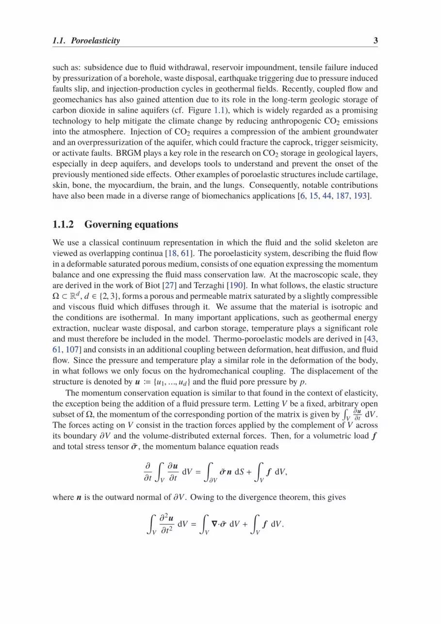
1.1.2 Governing equations
We use a classical continuum representation in which the fluid and the solid skeleton areviewed as overlapping continua [1818, 6161]. The poroelasticity system, describing the fluid flowin a deformable saturated porous medium, consists of one equation expressing the momentumbalance and one expressing the fluid mass conservation law. At the macroscopic scale, theyare derived in the work of Biot [2727] and Terzaghi [190190]. In what follows, the elastic structureΩ ⊂ Rd , d ∈ 2, 3, forms a porous and permeable matrix saturated by a slightly compressibleand viscous fluid which diffuses through it. We assume that the material is isotropic andthe conditions are isothermal. In many important applications, such as geothermal energyextraction, nuclear waste disposal, and carbon storage, temperature plays a significant roleand must therefore be included in the model. Thermo-poroelastic models are derived in [4343,6161, 107107] and consists in an additional coupling between deformation, heat diffusion, and fluidflow. Since the pressure and temperature play a similar role in the deformation of the body,in what follows we only focus on the hydromechanical coupling. The displacement of thestructure is denoted by u ≔ u1, ..., ud and the fluid pore pressure by p.
The momentum conservation equation is similar to that found in the context of elasticity,the exception being the addition of a fluid pressure term. Letting V be a fixed, arbitrary opensubset of Ω, the momentum of the corresponding portion of the matrix is given by
∫
V
∂u∂t
dV .The forces acting on V consist in the traction forces applied by the complement of V acrossits boundary ∂V and the volume-distributed external forces. Then, for a volumetric load f
and total stress tensor σ , the momentum balance equation reads
∂
∂t
∫
V
∂u
∂tdV =
∫
∂V
σn dS +
∫
V
f dV,
where n is the outward normal of ∂V . Owing to the divergence theorem, this gives
∫
V
∂2u
∂t2dV =
∫
V
∇·σ dV +
∫
V
f dV .

4 Chapter 1. Introduction
In the classical poroelasticity model, since the deformation of the material is usually muchslower than the flow rate, the inertial effects are considered negligible. This quasi-staticassumption consists in ignoring the second time-derivative for displacements and, since V
was chosen arbitrarily, it follows that
−∇·σ = f in Ω. (1.1)
Turning to the mass conservation equation, the variables of interest are the fluid contentη (fluid mass per unit bulk volume of porous medium), the flux w (fluid mass flow rate perunit area and time), and the volumetric fluid source g. Taking V ⊂ Ω as before, the rate atwhich fluid moves across the boundary ∂V is given by
∫
∂Vw ·n dS. Then the conservation of
mass for isothermal single-phase flow of a slightly compressible fluid takes the integral form
∂
∂t
∫
V
η dV +
∫
∂V
w ·n dS =
∫
V
g dV .
The divergence theorem applied to the second term of the left-hand side of the above equationand the fact that V was chosen arbitrarily lead to
∂η
∂t+ ∇·w = g. (1.2)
The coupling between the mechanical behavior of the matrix and the fluid dynamics isrealized by constitutive relations relating the total stress σ , the flux w , and the fluid content ηto the primary variables u and p. The total stress must account for the usual material stress,as in solid mechanics, and for the fluid pressure. Owing to the Terzaghi decomposition of thetotal stress [190190], one has
σ = σ − αpI d, (1.3)
whereσ is referred to as the effective stress tensor and measures the material properties of themedium. The Biot–Willis coefficient 0 < α ≤ 1, defined as the ratio of the volume changeof the fluid over the volume change of the medium, accounts for the pressure-deformationinteraction, and I d denotes the d-dimensional identity matrix. The effective stress tensordepends on the deformation according to the stress-strain relation σ = σ (∇su ), where thesymmetric gradient operator measures the strain in the case of small deformations and isdefined as
∇su ≔∇u + (∇u )T
2, with (∇u )i j ≔
∂ui
∂x j
, for 1 ≤ i, j ≤ d.
The standard assumption of Darcy’s law for porous media holds for the flux:
w = −K∇p
µf, (1.4)
where K is the tensor-valued intrinsic permeability field and µf is the fluid viscosity. Thethird constitutive assumption links the change in the fluid content η with the changes in the

1.1. Poroelasticity 5
fluid pressure p and and the material volume, which is locally measured by ∇·u . Morespecifically, following [6161, 6868], we set
η = c0p + α∇·u, (1.5)
where the Biot–Willis coefficient α quantifies the amount of fluid that can be forced into themedium by a variation of pore volume for a constant fluid pressure, while the constrainedspecific storage coefficient c0 ≥ 0 measures the amount of fluid that can be forced into themedium by pressure increments due to the compressibility of the structure. The case of asolid matrix with incompressible grains corresponds to the limit value c0 = 0.
1.1.3 The Biot model
The Biot model of linear poroelasticity is valid under the following assumptions: (i) smallrelative variations of porosity with respect to the equilibrium value ϕ ∈ [0, 1], (ii) smallrelative variations of the fluid density, and (iii) infinitesimal strain theory. Moreover, thematerial is assumed to be isotropic, linearly elastic, and homogeneous and, as a consequence,its mechanical behavior is described by Hooke’s stress-strain law
σ (∇su ) ≔ 2µ∇su + λ(∇·u )I d, (1.6)
the Lamé’s parameters µ > 0 and λ > 0 correspond to the dilatation and shear moduli,respectively. We recall that the shear modulus µ remains bounded and bounded away from0, namely 0 < µ ≤ µ ≤ µ ∈ R, whereas λ can take unboundedly large values in the case of aquasi-incompressible material (λ → ∞). We note that the condition λ > 0 is stronger thanthe one required to have the coercivity of the elasticity operator in Section 2.2.22.2.2. Indeed,λ ≥ − 2
dµ is sufficient to ensure the positivity of the bulk modulus and the well-posedness of
the weak formulation (5.185.18) (see also Lemma 5.45.4 and [178178]).The Biot model is derived by inserting the constitutive relations (1.31.3), (1.41.4), and (1.51.5)
into (1.11.1) and (1.21.2). Additional details on the model derivation and investigations on theporomechanical coefficient are given in Section 5.25.2. Hence, for a given bounded connecteddomain Ω ⊂ Rd , d ∈ 2, 3, with boundary ∂Ω and outward normal n, a finite time tF > 0,a volumetric load f , and a fluid source g, the corresponding problem consists in finding avector-valued displacement field u : Ω× (0, tF] → Rd and a scalar-valued pore pressure fieldp : Ω × (0, tF] → R solution of
−∇·σ (∇su ) + α∇p = f in Ω × (0, tF], (1.7a)
c0dt p + αdt (∇·u ) − ∇·(κ∇p) = g in Ω × (0, tF], (1.7b)
where dt denotes the time-derivative operator and κ ≔ K
µfthe tensor-valued fluid mobility
field. There are two distinct sets of boundary conditions, one corresponding to the deformationand one corresponding to the flow, and an initial condition on the fluid content to be added
6 Chapter 1. Introduction
to the above equations to close the model for the Biot problem:
u = uD on ΓD × (0, tF], (1.7c)
(σ (∇su ) + αpI d)n = tN on ΓN × (0, tF], (1.7d)
p = pd on Γd × (0, tF], (1.7e)
κ∇p · n = wn on Γn × (0, tF], (1.7f)
(c0p + α∇·u )(·, 0) = η0 in Ω, (1.7g)
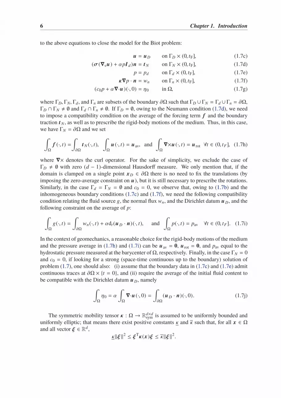
where ΓD, ΓN, Γd , and Γn are subsets of the boundary ∂Ω such that ΓD ∪ ΓN = Γd ∪ Γn = ∂Ω,ΓD ∩ ΓN , ∅ and Γd ∩ Γn , ∅. If ΓD = ∅, owing to the Neumann condition (1.7d1.7d), we needto impose a compatibility condition on the average of the forcing term f and the boundarytraction tN , as well as to prescribe the rigid-body motions of the medium. Thus, in this case,we have ΓN = ∂Ω and we set
∫
Ω
f (·, t) =∫
∂Ω
tN (·, t),∫
Ω
u (·, t) = uav, and
∫
Ω
∇×u (·, t) = u rot ∀t ∈ (0, tF], (1.7h)
where ∇× denotes the curl operator. For the sake of simplicity, we exclude the case ofΓD , ∅ with zero (d − 1)-dimensional Hausdorff measure. We only mention that, if thedomain is clamped on a single point xD ∈ ∂Ω there is no need to fix the translations (byimposing the zero-average constraint on u), but it is still necessary to prescribe the rotations.Similarly, in the case Γd = ΓN = ∅ and c0 = 0, we observe that, owing to (1.7b1.7b) and theinhomogeneous boundary conditions (1.7c1.7c) and (1.7f1.7f), we need the following compatibilitycondition relating the fluid source g, the normal flux wn, and the Dirichlet datum uD, and thefollowing constraint on the average of p:
∫
Ω
g(·, t) =∫
∂Ω
wn(·, t) + αdt (uD · n)(·, t), and
∫
Ω
p(·, t) = pav ∀t ∈ (0, tF]. (1.7i)
In the context of geomechanics, a reasonable choice for the rigid-body motions of the mediumand the pressure average in (1.7h1.7h) and (1.7i1.7i) can be uav = 0, u rot = 0, and pav equal to thehydrostatic pressure measured at the barycenter ofΩ, respectively. Finally, in the case ΓN = 0and c0 = 0, if looking for a strong (space-time continuous up to the boundary) solution ofproblem (1.71.7), one should also: (i) assume that the boundary data in (1.7c1.7c) and (1.7e1.7e) admitcontinuous traces at ∂Ω × t = 0, and (ii) require the average of the initial fluid content tobe compatible with the Dirichlet datum uD, namely
∫
Ω
η0 = α
∫
Ω
∇·u (·, 0) =
∫
∂Ω
(uD · n)(·, 0). (1.7j)
The symmetric mobility tensor κ : Ω → Rd×dsym is assumed to be uniformly bounded and
uniformly elliptic; that means there exist positive constants κ and κ such that, for all x ∈ Ωand all vector ξ ∈ Rd ,
κ‖ξ ‖2 ≤ ξTκ (x)ξ ≤ κ‖ξ ‖2.
1.1. Poroelasticity 7
Parameter Description Unit
µ ∈ [µ, µ] Shear modulus Paλ ∈ (0,+∞) Dilatation modulus Paκ ∈ Rd×d
sym Uniformly elliptic mobility tensor m2s−1Pa−1
ϕ ∈ [0, 1] Reference porosity value –α ∈ (ϕ, 1] Biot–Willis coefficient –c0 ≥ 0 Constrained specific storage coefficient Pa−1
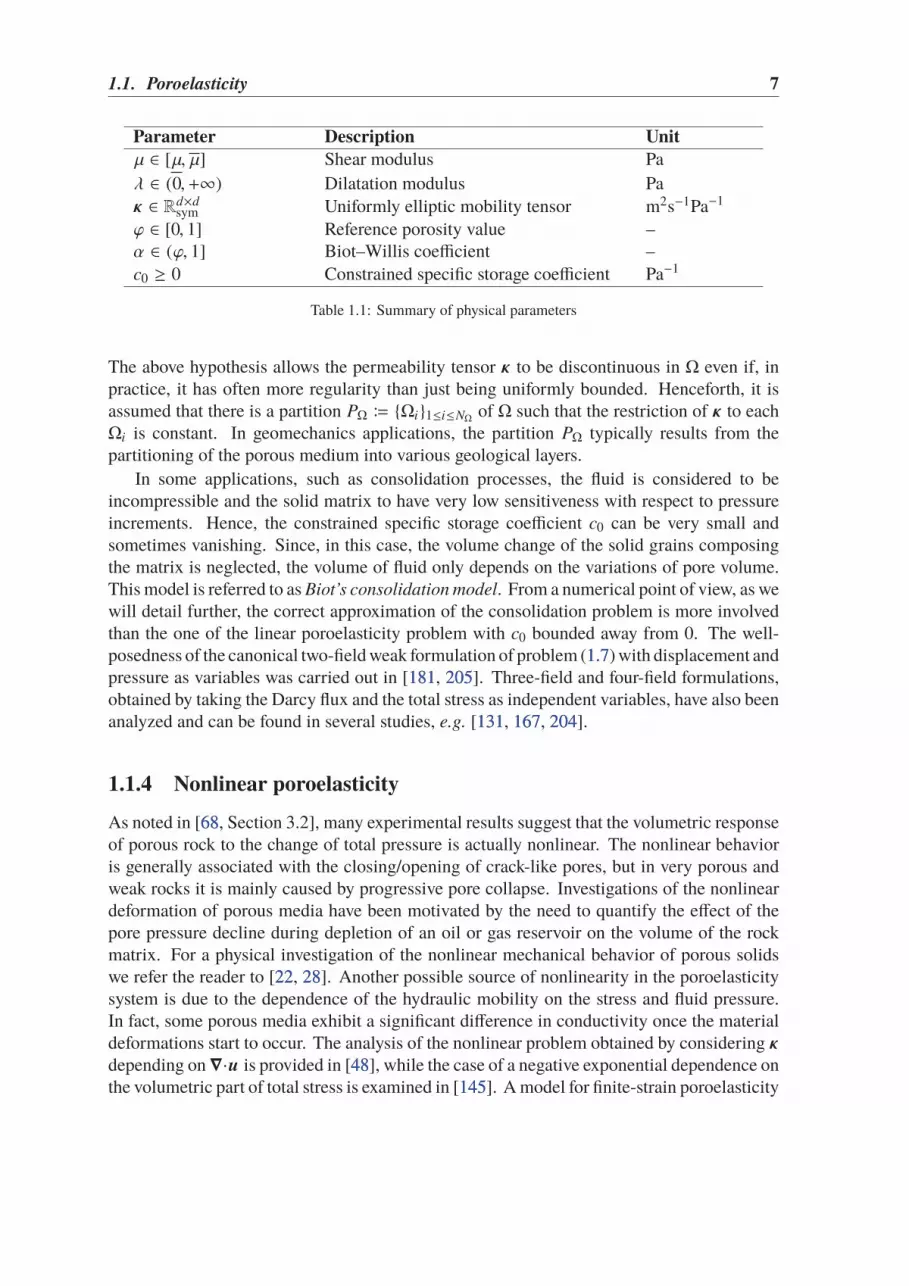
Table 1.1: Summary of physical parameters
The above hypothesis allows the permeability tensor κ to be discontinuous in Ω even if, inpractice, it has often more regularity than just being uniformly bounded. Henceforth, it isassumed that there is a partition PΩ ≔ Ωi1≤i≤NΩ of Ω such that the restriction of κ to eachΩi is constant. In geomechanics applications, the partition PΩ typically results from thepartitioning of the porous medium into various geological layers.
In some applications, such as consolidation processes, the fluid is considered to beincompressible and the solid matrix to have very low sensitiveness with respect to pressureincrements. Hence, the constrained specific storage coefficient c0 can be very small andsometimes vanishing. Since, in this case, the volume change of the solid grains composingthe matrix is neglected, the volume of fluid only depends on the variations of pore volume.This model is referred to as Biot’s consolidation model. From a numerical point of view, as wewill detail further, the correct approximation of the consolidation problem is more involvedthan the one of the linear poroelasticity problem with c0 bounded away from 0. The well-posedness of the canonical two-field weak formulation of problem (1.71.7) with displacement andpressure as variables was carried out in [181181, 205205]. Three-field and four-field formulations,obtained by taking the Darcy flux and the total stress as independent variables, have also beenanalyzed and can be found in several studies, e.g. [131131, 167167, 204204].
1.1.4 Nonlinear poroelasticity
As noted in [6868, Section 3.2], many experimental results suggest that the volumetric responseof porous rock to the change of total pressure is actually nonlinear. The nonlinear behavioris generally associated with the closing/opening of crack-like pores, but in very porous andweak rocks it is mainly caused by progressive pore collapse. Investigations of the nonlineardeformation of porous media have been motivated by the need to quantify the effect of thepore pressure decline during depletion of an oil or gas reservoir on the volume of the rockmatrix. For a physical investigation of the nonlinear mechanical behavior of porous solidswe refer the reader to [2222, 2828]. Another possible source of nonlinearity in the poroelasticitysystem is due to the dependence of the hydraulic mobility on the stress and fluid pressure.In fact, some porous media exhibit a significant difference in conductivity once the materialdeformations start to occur. The analysis of the nonlinear problem obtained by considering κdepending on∇·u is provided in [4848], while the case of a negative exponential dependence onthe volumetric part of total stress is examined in [145145]. A model for finite-strain poroelasticity

8 Chapter 1. Introduction
with deformation dependent permeability field has been proposed and analyzed in [2323, 9090].In this manuscript we focus on nonlinearities of the stress-strain relation σ : Ω×Rd×d
sym →R
d×dsym in the small deformation regime. In particular, in Chapter 44 we study the poroelasticity
problem obtained by replacing (1.61.6) with the hyperelastic nonlinear laws considered inChapter 33. Hyperelasticity is a type of constitutive model for ideally elastic materials inwhich the stress is determined by the current state of deformation by deriving a stored energydensity function Ψ : Rd×d
sym → R, namely
σ (τ) ≔∂Ψ(τ)
∂τ.
We next discuss a number of meaningful examples.Example 1.1 (Hencky–Mises model). The nonlinear Hencky–Mises model of [105105, 157157]corresponds to the stored energy density function
Ψhm(τ) ≔α
2tr(τ)2
+ Φ(dev(τ)), (1.8)
where dev : Rd×dsym → R defined by dev(τ) = tr(τ2)− 1
dtr(τ)2 is the deviatoric operator. Here,
α ∈ (0,+∞) and Φ : [0,+∞) → R is a function of class C2 satisfying, for some positiveconstants C1, C2, and C3,
C1 ≤ Φ′(ρ) < α, |ρΦ′′(ρ) | ≤ C2 and Φ′(ρ) + 2ρΦ′′(ρ) ≥ C3 ∀ρ ∈ [0,+∞). (1.9)
We observe that taking α = λ + 2dµ and Φ(ρ) = µρ in (1.81.8) leads to the linear case (1.61.6).
Deriving the energy density function (1.81.8) yields
σ (τ) = λ(dev(τ)) tr(τ)I d + 2µ(dev(τ))τ, (1.10)
with nonlinear Lamé functions µ(ρ) ≔ Φ′(ρ) and λ(ρ) ≔ α − Φ′(ρ).In the previous example the nonlinearity of the model only depends on the deviatoric part
of the strain. In the following model it depends on the term τ : Cτ.Example 1.2 (An isotropic reversible damage model). The isotropic reversible damage modelof [5050] can also be interpreted in the framework of hyperelasticity by setting up the energydensity function as
Ψdam(τ) ≔(1 − D(τ))
2τ : Cτ + Φ(D(τ)), (1.11)
where D : Rd×dsym → [0, 1] is the scalar damage function and C is a fourth-order symmetric
and uniformly elliptic tensor, namely, for some positive constants C∗ and C∗, it holds
C∗‖τ‖2d×d ≤ Cτ : τ ≤ C∗‖τ‖2
d×d, ∀τ ∈ Rd×d . (1.12)
The function Φ : [0, 1] → R defines the relation between τ and D by ∂φ∂D=
12τ : Cτ. The
resulting stress-strain relation reads
σ (τ) = (1 − D(τ))Cτ. (1.13)

1.2. Discretization 9
Another generalization of the linear stress-strain relation is obtained by adding second-order terms to (1.61.6).Example 1.3 (A second-order elasticity model). In the second-order isotropic elasticity modelof [6666, 124124] the stress-strain relation is
σ (τ) = λ tr(τ)I d + 2µτ + B tr((τ)2)I d + 2B tr(τ)τ + C tr(τ)2I d + A(τ)2, (1.14)
where λ and µ are the standard Lamé parameter, and A, B,C ∈ R are the second-order moduli.We note that the hyperelastic stored energy function associated to the the stress-strain relation(1.141.14) has third-order terms and in general is not polyconvex, i.e. convex with respect to eachof the strain invariants.
1.2 Discretization
In order to discretize the Biot and nonlinear poroelasticity problems presented in the previoussections, we consider a coupling of the Hybrid High-Order (HHO) and discontinuous Galerkin(dG) method. Concerning the time discretization, we consider backward differentiationformulas (especially the implicit Euler method), which are the simplest and most widely usedmethods in the literature. We show that this construction yields an inf-sup stable hydro-mechanical coupling, which is a crucial property to ensure robustness for small time stepscombined with small permeabilities. Additionally, the analysis presented in Chapter 22 and44 allows to derive error estimates that are robust in the limit c0 → 0 which, as noted inSection 1.2.11.2.1 and in [164164, Section 5.2], is expected to mitigate the problem of the nonphysicalpressure oscillations which can sometimes arise in the numerical simulation of poroelasticsystems. Before discussing the main features of the discretization methods considered in thenext chapters, we give an overview of the numerical issues related to the discretization ofporoelasticity problems.
1.2.1 Numerical issues
Several difficulties have to be accounted for in the design of a discretization methods forproblem (1.71.7). These issues have three origins: the discretization of the elasticity operator,the (possibly saddle-point) coupling between the flow and the mechanics, and the roughvariations of the permeability coefficient that the Darcy operator has to accomodate.
First, we remark that the elasticity operator has to be carefully engineered in order to ensurestability expressed by a discrete version of Korn’s inequality. Conforming finite elementsnaturally yields coercive discretizations, but this is not necessarily the case when consideringnonconforming approximations. For instance, it is well known that the Crouzeix–Raviartspace (spanned by piecewise affine functions that are continuous at the midpoint of meshinterfaces) does not fulfill a discrete Korn’s inequality. Another numerical issue concerningthe discretization of elasticity problems is the so-called locking phenomenon. When thedilatation modulus λ in (1.61.6) is very large, which corresponds to a quasi-incompressiblematerial, results of poor quality can be obtained. More specifically, it can be observed that

10 Chapter 1. Introduction
the material deforms as if it were much stiffer. In other words, it appears to lock. The keypoint to ensure that a numerical method is locking-free is to establish an error estimate witha multiplicative constant not blowing up in the limit λ → ∞, i.e. being able to prove uniformconvergence with respect to λ.
The stability of the saddle-point mechanics-flow coupling is closely related to the elasticitylocking phenomenon. Indeed, for both of them, the difficulty lies in the approximationof the divergence operator. In the linear elasticity context, locking can be handled byprojecting the divergence operator onto a discrete (pressure) space which satisfies an inf-supcondition when coupled with the displacement approximation space. In the context of aporoelastic displacement-pressure coupling, stability can thus be obtained by considering adiscrete pressure belonging to that space, which is in fact equivalent to projecting the discretedivergence operator onto the pressure space in the coupling term. From a mathematicalpoint of view, the inf-sup condition yields an estimate in the L∞((0, tF); L2(Ω))-norm on thediscrete pore pressure which is independent of κ−1. It is of some importance to note thatinf-sup stability is not strictly needed in the compressible case (i.e. with c0 > 0). As a matterof fact, the presence of the term c0dt p in the left-hand side of the fluid balance Equation(1.7b1.7b) directly yields a discrete L∞((0, tF); L2(Ω)) estimate on the pore pressure which doesnot depend neither on κ−1 nor on λ. An investigation of the role of the inf-sup conditionin the context of finite element discretizations of linear poroelasticity can be found, e.g. ,in [154154, 155155] and in [165165, 166166].
The problem of spurious spatial oscillations of the pore pressure is actually more involvedthan a simple saddle-point coupling issue. The difficulty comes from the fact that, in veryearly times (or when the permeability is low), the pressure is quasi-L2(Ω) as the diffusionterm gives an almost vanishing contribution. However, as soon as t > 0, boundary conditionsare imposed on the pore pressure hence giving necessarily to this latter a H1(Ω) regularity.When c0 = 0, if no discrete inf-sup condition holds, the only control of pressure is given bythe diffusion term, which is almost inexistent in early times. Spurious spatial oscillations thenarise. If an inf-sup condition holds, then it yields a control of the pressure approximation,hence reducing the oscillations. However, it has been recently pointed out in [176176] that, evenfor discretization methods leading to an inf-sup stable discretization of the Stokes problem inthe steady case, pressure oscillations can arise owing to a lack of monotonicity of the discreteoperator.
1.2.2 Polyhedral element methods
In recent years, a large effort has been devoted to the development and analysis of numericalmethods that apply to more general meshes than simplicial or Cartesian ones. In the contextof poroelaticity, this necessity arises from the presence of various layers and fractures inthe porous medium. The discretization of the domain may also include degenerate elements(as in the near wellbore region in reservoir modelling, e.g. Figure 1.21.2) and nonconforminginterfaces (accounting for the presence of cracks or resulting from local mesh refinement).In the context of structural mechanics, discretization methods supporting polyhedral meshesand nonconforming interfaces can be useful for several reasons including, e.g., the use ofhanging nodes for contact and interface elasticity problems, and the greater robustness to mesh

1.2. Discretization 11
Figure 1.2: Example of polyhedral mesh with degenerate elements in reservoir applications
distorsion and fracture. Moreover, polyhedral methods allow for simple mesh refinement andcoarsening procedures for adaptivity.
In this dissertation, we focus on two families of polyhedral discretization methods: theHHO and dG methods. Both are nonconforming in the context of primal formulations of ellip-tic problems, since no continuity condition is imposed between neighboring mesh elements.They are also high-order methods, because they allow to increase the space approximation or-der. The use of high-order methods can classically accelerate the convergence in the presenceof regular exact solutions or when combined with local mesh refinement. Additionally, theconstruction of discrete problems using the HHO and dG discretizations is valid for arbitraryspace dimension and this enables dimension-independent implementations. In what follows,we consider the HHO method of [3333, 7474] for the discretization of the (possibly nonlinear)elasticity operator in (1.7a1.7a) and the Symmetric Weighted Interior Penalty (SWIP) dG methodof [7777, 9393] for the Darcy operator in (1.7b1.7b).
Discontinuous Galerkin methods can be viewed as finite element methods allowing fordiscontinuities in the discrete trial and test spaces. Localizing test functions to single meshelements, they can also be viewed as finite volume methods in which the approximatesolution is represented on each mesh element by a polynomial function and not only by aconstant function. Allowing the approximate solution to be only piecewise continuous offersa substantial amount of flexibility in the mesh design. A unified analysis of dG methodsfor elliptic problems can be found in [4242] and in [7676, Chapter 4]. The fundamental strategyto approximate heterogeneous diffusion (such us Darcean flow in porous media) problemusing dG methods is to penalize interface and boundary jumps using a diffusion-dependentparameter scaling as the harmonic mean of the normal component of the diffusion tensor.Indeed, using the harmonic mean to penalize will turn out to tune automatically the amountof penalty. Moreover, as pointed out in Chapter 44 and in [7777] the proposed method is robustwith respect to the spatial variations of the permeability coefficient, with constants in theerror estimates having a mild dependendance on the heterogeneity ratio.
Hybrid High-Order methods, introduced in [7878] and [7474], rely on primal formulations ofelliptic problems and lead to a symmetric, positive definite system matrices. The methods canbe deployed on general polyhedral meshes. The degrees of freedom are polynomials of thesame order at mesh elements and faces: face-based discrete unknowns establish inter-elementsconnections at interfaces and can be used to strongly enforce essential boundary conditions
12 Chapter 1. Introduction
at boundary faces, element-based discrete unknowns are intermediate variables which canbe eliminated from the global system by static condensation, as detailed in [5757, Section2.4] and in Section 2.52.5. The design of these methods proceeds in two step: (i) the discretereconstructions of differential operators hinging on the solution of inexpensive local problemsinside each element and (ii) the definition of a least-squares stabilization that weakly enforcesthe matching of element- and face-based discrete unknowns. The definitions of the differentialreconstructions operators are based on discrete counterparts of integrations by parts. Even iflocal problems related to the reconstruction operators have to be solved, the numerical resultsof [7474] indicate that the associated cost becomes marginal with respect to the cost of solvingthe global systems as the number of discrete unknowns is increased. Moreover, HHO methodsare computationally effective, since the use of face unknowns yields to compact stencils, andthey can be efficiently implemented thanks to the possibility of statically condensing a largesubset of the unknowns. The HHO discretization studied in Chapter 33 for nonlinear elasticityproblems is inspired by recent works on Leray–Lions operators [6969, 7070], where the authorsshow that the method is robust with respect to nonlinearities. The robustness of the methodwith respect to locking has been proved in [7474, Section 5].
Other locking-free polyhedral schemes have been proposed for the discretization of linearelasticity problems. A non-exhaustive list includes: (i) the Hybridizable discontinuousGalerkin (HDG) method of [185185], (ii) the Mimetic Finite Difference (MFD) scheme of [1919],(iii) the Virtual Element Method (VEM) of [2020], (iv) the generalized Crouzeix–Raviartscheme introduced in [8080], and (v) the Weak Galerkin (WG) method of [197197]. Concerningthe nonlinear version of the problem, discretization methods supporting general meshes havealso been considered in [2121] and [5454], where the authors propose a low-order VEM schemefor small and finite deformations, respectively. The HHO method has been applied for thediscretization of finite deformations elasticity problems in [11]. To the best of our knowledge,the existing literature on the approximation of poroelasticity problem on general polyhedralmeshes is more scarce. We can cite the vectorial Multi-Point Flux Approximation methodsof [160160], the Hybrid Finite Volume discretization considered in [138138], and the very recentHDG method of [101101] .
1.3 Uncertainty quantification
In numerical simulation, accounting for uncertainties in input data (such as physical constants,boundary and initial conditions, external forcing, and geometry) is a crucial issue, especiallyin risk analysis, safety, and design. Risk assessment in poroelasticity is a critical challengefor a wide range of vital resource management applications. Recent public concerns overinduced seismicity [6363, 113113] and groundwater contamination [182182] underscore the need toquantify the probability of harmful events associated with subsurface flow and deformation.Of particular interest is the prediction of critical stresses which can compromise the caprockintegrity [162162] and wellbore stability [153153] in storage reservoirs. The key to successful riskassessment in these contexts is the ability to predict the probability of critical events basedon some empirical approximation of the material parameters and source term variability.For this reason there is a particular need to combine numerical methods for poromechanical

1.4. Plan of the manuscript 13
simulation with efficient techniques for quantifying uncertainties.Uncertainty Quantification (UQ) methods have been developed in the last decades to take
into account the effect of random input parameters on the quantity of interest. They enable toobtain information on the model output that is richer than in a deterministic context, since theyprovide the statistical moments and the probability distribution. This information makes thecomparison with experimental observation easier and facilitate the evaluation of the validityof the physical models. Indeed, UQ methods provide confidence intervals in computedpredictions and identify the uncertain parameters that should be measured or controlled withmore accuracy because they have the most significant impact on the solution. Additionally,they allow to assess the limits of predictability and the level of reliability that can be attachedto numerical simulations.
Among the techniques designed for UQ in numerical models, the stochastic spectralmethods have received a considerable attention. The core idea of these methods is thedecomposition of random quantities on suitable approximation bases such as the Karhunen–Loéve [142142, 180180] or the Polynomial Chaos [112112, 137137] expansions. The former represents therandom fields as a linear combination of an infinite number of uncorrelated random variables,while the latter uses polynomial expansions in terms of independent random variables. Theirmain interest is that they provide a complete probabilistic description of the uncertain solution.
In Chapter 55, in order to investigate the effect of uncertainty in poroelasticity problems,we rely on a Polynomial Chaos (PC) approach. The fundamental concept on which PCdecompositions are based is to regard uncertainty as generating a new dimension and thesolution as being dependent on this dimension. A convergent expansion along the newdimension is then sought in terms of a set of orthogonal basis functions, whose coefficientscan be used to characterize the uncertainty. The motivation behind PC approaches includes:(i) the suitability to model expressed in terms of partial differential equations, (ii) the ability todeal with situations exhibiting steep nonlinear dependence of the solution on random modeldata, and (iii) the promise of obtaining efficient and accurate estimates of uncertainty. Inaddition, the provided information is given in a format that can be readily exploited to probethe dependence of specific observables on particular components of the input data.
1.4 Plan of the manuscript
The rest manuscript is organized as follows.In Chapter 22, published in SIAM Journal on Scientific Computing (cf. [3030]), we introduce
a novel algorithm for the Biot problem based on a HHO discretization of the mechanics anda Symmetric Weighted Interior Penalty dG discretization of the flow. The method hasseveral assets, including, in particular, the validity in two and three space dimensions, inf-sup stability, and the support of general polyhedral meshes, nonmatching interfaces, andarbitrary space approximation order. Additionally, the resolution cost can be reduced bystatically condensing a large subset of the unknowns. Our analysis delivers stability and errorestimates that hold also when the constrained specific storage coefficient vanishes, and showsthat the constants have only a mild dependence on the heterogeneity of the permeabilitycoefficient. We discuss implementation details and provide numerical tests demonstrating

14 Chapter 1. Introduction
the performance of the method. In particular, we numerically check the robustness of themethod with respect to pressure spurious oscillations. Finally, we show that the scheme islocally conservative on the primal mesh, a desirable property for practitioners and key for aposteriori estimates based on equilibrated fluxes.
In Chapter 33, published in SIAM Journal on Numerical Analysis (cf. [3333]), we propose andanalyze a novel HHO discretization of a class of (linear and) nonlinear elasticity models in thesmall deformation regime which are of common use in solid mechanics. The method satisfiesa local principle of virtual work inside each mesh element, with interface tractions that obeythe law of action and reaction. A complete analysis covering very general stress-strain laws iscarried out. In particular, we prove the existence of a discrete solution and we identify a strictmonotonicity assumption on the stress-strain law which ensures uniqueness. Convergence tominimal regularity solutions u ∈ H1
0 (Ω;Rd) is proved using a compactness argument. Anoptimal energy-norm error estimate in hk+1 is then proved under the additional conditions ofLipschitz continuity and strong monotonicity on the stress-strain law. The performance of themethod is extensively investigated on a complete panel of model problems using stress-strainlaws corresponding to real materials. The numerical tests show that the method is robustwith respect to strong nonlinearities.
In Chapter 44, building on the material of the previous chapters, we construct and analyzea coupled HHO-dG discretization method for the nonlinear poroelasticity problem. Thechapter is submitted for publication (see [3535] for the preprint version). Compared to themethod proposed in Chapter 22 for the linear poroelasticity problem, there are two maindifferences in the design. First, the discrete symmetric gradient sits in the full space oftensor-valued polynomials, as opposed to symmetric gradients of vector-valued polynomials.As shown in Chapter 33, this modification is required for the convergence analysis in thepresence of nonlinear stress-strain laws. Second, the right-hand side of the discrete problemis obtained by taking the average in time of the loading force f and fluid source g betweentwo consecutive time steps. This modification allows us to prove stability and optimal errorestimates without any additional time regularity assumptions on data. Moreover, the resultsholds for both nonzero and vanishing storage coefficients. In this chapter we also give a newsimple proof of discrete Korn’s inequality, not requiring particular geometrical assumptionson the mesh.
In Chapter 55, we consider the numerical solution of the Biot problem with randomporoelastic coefficients in the context of uncertainty quantification. The chapter collects partof the ongoing work carried out during the internship at the BRGM that took place fromJanuary to September 2018. The uncertainty is modelled with a finite set of parameters withprescribed probability distribution. We present the variational formulation of the stochasticpartial differential system and establish its well-posedness. We then discuss the approximationof the parameter-dependent problem by non-intrusive techniques based on on PolynomialChaos decompositions. We specifically focus on sparse spectral projection methods whichessentially amount to performing an ensemble of deterministic model simulations to estimatethe expansion coefficients. We numerically investigate the convergence of the probabilityerror of the PC approximation with respect to the level of the sparse grid. Finally, we performa sensitivity analysis to asses the propagation of the input uncertainty on the solutions
1.4. Plan of the manuscript 15
considering an injection test and a traction problem.In Appendix AA, published in the conference book Finite Volumes for Complex Appli-
cations VIII (cf. [3434]), we present a variant of the HHO-dG algorithm for the quasi-staticnonlinear poroelasticity problem studied in Chapter 44. In particular, this appendix providesnumerical tests demonstrating the convergence of the method considering the Hencky-Misesnon-linear behavior law.
Appendix BB is an excerpt of a complementary work that has been published in Computa-
tional Methods in Applied Mathematics (cf. [3636]). I decided not to include the full version togive a more consistent structure to the manuscript. Therein we consider hyperelastic problemsand their numerical solution using a conforming finite element discretization and iterativelinearization algorithms. For these problems, we present equilibrated, weakly symmetric,H (div)-conforming stress tensor reconstructions, obtained from local problems on patchesaround vertices using the Arnold–Falk–Winther finite element spaces. We distinguish twostress reconstructions, one for the discrete stress and one representing the error of the itera-tive linearization algorithm. The reconstructions are independent of the mechanical behaviorlaw. Based on these stress tensor reconstructions, we derive an a posteriori error estimatedistinguishing the discretization, linearization, and quadrature error estimates, and proposean adaptive algorithm balancing these different error sources. We prove the efficiency ofthe estimate, and confirm it on a numerical test with analytical solution. We then apply theadaptive algorithm to a more application-oriented test.

16 Chapter 1. Introduction

Chapter 2
The Biot problem
This chapter has been published in the following peer-reviewed journal (see [3030]):
SIAM Journal on Scientific Computing,Volume 38, Issue 3, 2016, Pages A1508–A1537.
Contents
2.1 Introduction . . . . . . . . . . . . . . . . . . . . . . . . . . . . . . . . 1818
2.2 Discretization . . . . . . . . . . . . . . . . . . . . . . . . . . . . . . . . 2020
2.2.1 Mesh and notation . . . . . . . . . . . . . . . . . . . . . . . . . 2020
2.2.2 Linear elasticity operator . . . . . . . . . . . . . . . . . . . . . . 2222
2.2.3 Darcy operator . . . . . . . . . . . . . . . . . . . . . . . . . . . 2424
2.2.4 Hydro-mechanical coupling . . . . . . . . . . . . . . . . . . . . 2525
2.2.5 Formulation of the method . . . . . . . . . . . . . . . . . . . . . 2626
2.3 Stability analysis . . . . . . . . . . . . . . . . . . . . . . . . . . . . . . 2727
2.4 Error analysis . . . . . . . . . . . . . . . . . . . . . . . . . . . . . . . 3131
2.4.1 Projection . . . . . . . . . . . . . . . . . . . . . . . . . . . . . . 3131
2.4.2 Error equations . . . . . . . . . . . . . . . . . . . . . . . . . . . 3333
2.4.3 Convergence . . . . . . . . . . . . . . . . . . . . . . . . . . . . 3333
2.5 Implementation . . . . . . . . . . . . . . . . . . . . . . . . . . . . . . 3737
2.6 Numerical tests . . . . . . . . . . . . . . . . . . . . . . . . . . . . . . . 4040
2.6.1 Convergence . . . . . . . . . . . . . . . . . . . . . . . . . . . . 4040
2.6.2 Barry and Mercer’s test case . . . . . . . . . . . . . . . . . . . . 4242
2.7 Appendix: Flux formulation . . . . . . . . . . . . . . . . . . . . . . . 4444
17
18 Chapter 2. The Biot problem
2.1 Introduction
We consider in this chapter the quasi-static Biot’s consolidation problem describing Darcianflow in a deformable saturated porous medium. Our original motivation comes from appli-cations in geosciences, where the support of general polyhedral meshes is crucial, e.g., tohandle nonconforming interfaces arising from local mesh adaptation or Voronoi elements inthe near wellbore region when modelling petroleum extraction. Let Ω ⊂ Rd , 1 ≤ d ≤ 3,denote a bounded connected polyhedral domain with boundary ∂Ω and outward normal n.For a given finite time tF > 0, volumetric load f , fluid source g, the Biot problem consists infinding a vector-valued displacement field u and a scalar-valued pore pressure field p solutionof
−∇·σ (u ) + α∇p = f in Ω × (0, tF), (2.1a)
c0dt p + ∇·(αdtu ) − ∇·(κ∇p) = g in Ω × (0, tF), (2.1b)
where c0 ≥ 0 and α > 0 are real numbers corresponding to the constrained specific storageand Biot–Willis coefficients, respectively, κ is a real-valued permeability field such thatκ ≤ κ ≤ κ a.e. in Ω for given real numbers 0 < κ ≤ κ , and the Cauchy stress tensor is givenby
σ (u ) ≔ 2µ∇su + λI d∇·u,
with real numbers λ ≥ 0 and µ > 0 corresponding to Lamé’s parameters, ∇s denoting thesymmetric part of the gradient operator applied to vector-valued fields, and I d denoting theidentity matrix of Rd×d . Equations (2.1a2.1a) and (2.1b2.1b) express, respectively, the mechanicalequilibrium and the fluid mass balance. We consider, for the sake of simplicity, the followinghomogeneous boundary conditions:
u = 0 on ∂Ω × (0, tF), (2.1c)
κ∇p · n = 0 on ∂Ω × (0, tF). (2.1d)
Initial conditions are set prescribing u (·, 0) = u0 and, if c0 > 0, p(·, 0) = p0. In theincompressible case c0 = 0, we also need the following compatibility condition on g:
∫
Ω
g(·, t) = 0 ∀t ∈ (0, tF), (2.1e)
as well as the following zero-average constraint on p:
∫
Ω
p(·, t) = 0 ∀t ∈ (0, tF). (2.1f)
For the derivation of the Biot model we refer to the seminal work of Terzaghi [190190] andBiot [2727, 2929]. A theoretical study of problem (2.12.1) can be found in [181181]. For the preciseregularity assumptions on the data and on the solution under which our a priori bounds andconvergence estimates are derived, we refer to Lemma 2.72.7 and Theorem 2.122.12, respectively.
2.1. Introduction 19
A few simplifications are made to keep the exposition as simple as possible while stillretaining all the principal difficulties. For the Biot–Willis coefficient we take
α = 1,
an assumption often made in practice. For the scalar-valued permeability κ , we assume thatit is piecewise constant on a partition PΩ of Ω into bounded open polyhedra. The treatmentof more general permeability coefficients can be done following the ideas of [7777]. Also, moregeneral boundary conditions than (2.1c2.1c)–(2.1d2.1d) can be considered up to minor modifications.
Our focus is here on a novel space discretization for the Biot problem (standard choices aremade for the time discretization). Several difficulties have to be accounted for in the design ofthe space discretization of problem (2.12.1): in the context of nonconforming methods, the linearelasticity operator has to be carefully engineered to ensure stability expressed by a discretecounterpart of the Korn’s inequality; the Darcy operator has to accomodate rough variationsof the permeability coefficient; the choice of discrete spaces for the displacement and thepressure must satisfy an inf-sup condition to contribute reducing spurious pressure oscillationsfor small time steps combined with small permeabilities when c0 = 0. An investigation of therole of the inf-sup condition in the context of finite element discretizations can be found, e.g.,in Murad and Loula [154154, 155155]. A recent work of Rodrigo, Gaspar, Hu, and Zikatanov [176176]has pointed out that, even for discretization methods leading to an inf-sup stable discretizationof the Stokes problem in the steady case, pressure oscillations can arise owing to a lack ofmonotonicity. Therein, the authors suggest that stabilizing is possible by adding to the massbalance equation an artificial diffusion term with coefficient proportional to h2/τ (with h andτ denoting, respectively, the spatial and temporal meshsizes). However, computing the exactamount of stabilization required is in general feasible only in 1 space dimension.
Several space discretization methods for the Biot problem have been considered in theliterature. Finite element discretizations are discussed, e.g., in the monograph of Lewisand Schrefler [140140]; cf. also references therein. A finite volume discretization for thethree-dimensional Biot problem with discontinuous physical coefficients is considered byNaumovich [156156]. In [165165, 166166], Phillips and Wheeler propose and analyze an algorithmthat models displacements with continuous elements and the flow with a mixed method.In [167167], the same authors also propose a different method where displacements are insteadapproximated using discontinuous Galerkin methods. In [200200], Wheeler, Xue and Yotovstudy the coupling of multipoint flux discretization for the flow with a discontinuous Galerkindiscretization of the displacements. While certainly effective on matching simplicial meshes,discontinuous Galerkin discretizations of the displacements usually do not allow to proveinf-sup stability on general polyhedral meshes.
In this chapter, we propose a novel space discretization of problem (2.12.1) where the linearelasticity operator is discretized using the Hybrid High-Order (HHO) method of [7474] (c.f.also [7171, 7373, 7878]), while the flow relies on the Symmetric Weighted Interior Penalty (SWIP)discontinuous Galerkin method of [7777], see also [7676, Chapter 4]. The proposed method hasseveral assets: (i) It delivers an inf-sup stable discretization on general meshes including,e.g., polyhedral elements and nonmatching interfaces; (ii) it allows to increase the spaceapproximation order to accelerate convergence in the presence of (locally) regular solutions;

20 Chapter 2. The Biot problem
(iii) it is locally conservative on the primal mesh, a desirable property for practitioners andkey for a posteriori estimates based on equilibrated fluxes; (iv) it is robust with respect to thespatial variations of the permeability coefficient, with constants in the error estimates thatdepend on the square root of the heterogeneity ratio; (v) it is (relatively) inexpensive: at thelowest order, after static condensation of element unknowns for the displacement, we have 4(resp. 9) unknowns per face for the displacements + 3 (resp. 4) unknowns per element for thepore pressure in 2d (resp. 3d). Finally, the proposed construction is valid for arbitrary spacedimension, a feature which can be exploited in practice to conceive dimension-independentimplementations.
The material is organized as follows. In Section 2.22.2, we introduce the discrete settingand formulate the method. In Section 2.32.3, we derive a priori bounds on the exact solu-tion for regular-in-time volumetric load and mass source. The convergence analysis of themethod is carried out in Section 2.42.4. Implementation details are discussed in Section 2.52.5,while numerical tests proposed in Section 2.62.6. Finally, in Appendix 2.72.7, we investigate thelocal conservation properties of the method by identifying computable conservative normaltractions and mass fluxes.
2.2 Discretization
In this section we introduce the assumptions on the mesh, define the discrete counterparts ofthe elasticity and Darcy operators and of the hydro-mechanical coupling terms, and formulatethe discretization method.
2.2.1 Mesh and notation
Denote by H ⊂ R+∗ a countable set of meshsizes having 0 as its unique accumulation point.Following [7676, Chapter 1], we consider h-refined spatial mesh sequences (Th)h∈H where, forall h ∈ H , Th is a finite collection of nonempty disjoint open polyhedral elements T suchthat Ω =
⋃
T∈Th T and h = maxT∈Th hT with hT standing for the diameter of the element T .We assume that mesh regularity holds in the following sense: For all h ∈ H , Th admits amatching simplicial submesh Th and there exists a real number > 0 independent of h suchthat, for all h ∈ H , (i) for all simplex S ∈ Th of diameter hS and inradius rS, hS ≤ rS and(ii) for all T ∈ Th, and all S ∈ Th such that S ⊂ T , hT ≤ hS. A mesh sequence with thisproperty is called regular. It is worth emphasizing that the simplicial submesh Th is just ananalysis tool, and it is not used in the actual construction of the discretization method. Theseassumptions are essentially analogous to those made in the context of other recent methodssupporting general meshes; cf., e.g., [2020, Section 2.2] for the Virtual Element method. For acollection of useful geometric and functional inequalities that hold on regular mesh sequenceswe refer to [7676, Chapter 1] and [6969].
Remark 2.1 (Face degeneration). The above regularity assumptions on the mesh imply thatthe diameter of the mesh faces is uniformly comparable to that of the cell(s) they belongto, i.e., face degeneration is not allowed. Face degeneration has been considered, on theother hand, in [4747] in the context of interior penalty discontinuous Galerkin methods. One
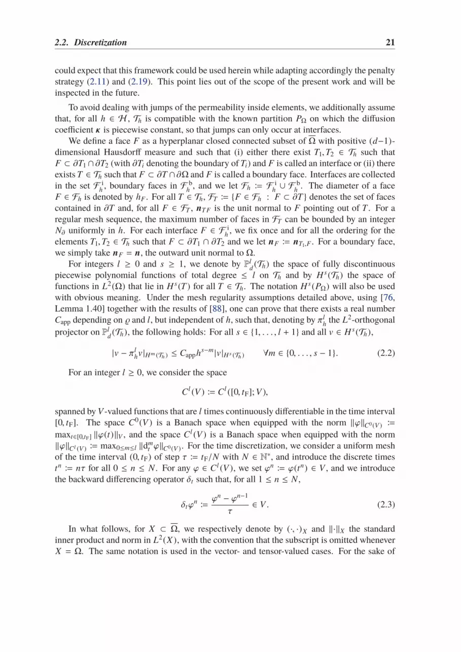
2.2. Discretization 21
could expect that this framework could be used herein while adapting accordingly the penaltystrategy (2.112.11) and (2.192.19). This point lies out of the scope of the present work and will beinspected in the future.
To avoid dealing with jumps of the permeability inside elements, we additionally assumethat, for all h ∈ H , Th is compatible with the known partition PΩ on which the diffusioncoefficient κ is piecewise constant, so that jumps can only occur at interfaces.
We define a face F as a hyperplanar closed connected subset of Ω with positive (d−1)-dimensional Hausdorff measure and such that (i) either there exist T1,T2 ∈ Th such thatF ⊂ ∂T1∩ ∂T2 (with ∂Ti denoting the boundary of Ti) and F is called an interface or (ii) thereexists T ∈ Th such that F ⊂ ∂T ∩∂Ω and F is called a boundary face. Interfaces are collectedin the set F i
h, boundary faces in F b
h, and we let Fh ≔ F i
h∪ F b
h. The diameter of a face
F ∈ Fh is denoted by hF . For all T ∈ Th, FT ≔ F ∈ Fh : F ⊂ ∂T denotes the set of facescontained in ∂T and, for all F ∈ FT , nT F is the unit normal to F pointing out of T . For aregular mesh sequence, the maximum number of faces in FT can be bounded by an integerN∂ uniformly in h. For each interface F ∈ F i
h, we fix once and for all the ordering for the
elements T1,T2 ∈ Th such that F ⊂ ∂T1 ∩ ∂T2 and we let nF ≔ nT1,F . For a boundary face,we simply take nF = n, the outward unit normal to Ω.
For integers l ≥ 0 and s ≥ 1, we denote by Pld(Th) the space of fully discontinuous
piecewise polynomial functions of total degree ≤ l on Th and by H s (Th) the space offunctions in L2(Ω) that lie in H s (T ) for all T ∈ Th. The notation H s (PΩ) will also be usedwith obvious meaning. Under the mesh regularity assumptions detailed above, using [7676,Lemma 1.40] together with the results of [8888], one can prove that there exists a real numberCapp depending on and l, but independent of h, such that, denoting by πl
hthe L2-orthogonal
projector on Pld(Th), the following holds: For all s ∈ 1, . . . , l + 1 and all v ∈ H s (Th),
|v − πlhv |Hm (Th ) ≤ Capphs−m |v |H s (Th ) ∀m ∈ 0, . . . , s − 1. (2.2)
For an integer l ≥ 0, we consider the space
Cl (V ) ≔ Cl ([0, tF]; V ),
spanned by V -valued functions that are l times continuously differentiable in the time interval[0, tF]. The space C0(V ) is a Banach space when equipped with the norm ‖ϕ‖C0(V ) ≔
maxt∈[0,tF] ‖ϕ(t)‖V , and the space Cl (V ) is a Banach space when equipped with the norm‖ϕ‖Cl (V ) ≔ max0≤m≤l ‖dm
t ϕ‖C0(V ). For the time discretization, we consider a uniform meshof the time interval (0, tF) of step τ ≔ tF/N with N ∈ N∗, and introduce the discrete timestn≔ nτ for all 0 ≤ n ≤ N . For any ϕ ∈ Cl (V ), we set ϕn
≔ ϕ(tn) ∈ V , and we introducethe backward differencing operator δt such that, for all 1 ≤ n ≤ N ,
δtϕn≔
ϕn − ϕn−1
τ∈ V . (2.3)
In what follows, for X ⊂ Ω, we respectively denote by (·, ·)X and ‖·‖X the standardinner product and norm in L2(X ), with the convention that the subscript is omitted wheneverX = Ω. The same notation is used in the vector- and tensor-valued cases. For the sake of

22 Chapter 2. The Biot problem
brevity, throughout the chapter, we will often use the notation a . b for the inequality a ≤ Cb
with generic constant C > 0 independent of h, τ, c0, λ, µ, and κ , but possibly depending on and the polynomial degree k. We will name generic constants only in statements or whenthis helps to follow the proofs.
2.2.2 Linear elasticity operator
The discretization of the linear elasticity operator is based on the Hybrid High-Order methodof [7474]. Let a polynomial degree k ≥ 1 be fixed. The degrees of freedom (DOFs) for thedisplacement are collected in the space
U kh≔
×T∈Th Pkd (T )d
××F∈Fh P
kd−1(F)d
.For a generic collection of DOFs in U k
hwe use the notation v
h≔
(
(vT )T∈Th, (vF )F∈Fh)
. Wealso denote by vh (not underlined) the function of Pk
d(Th)d such that vh |T = vT for all T ∈ Th.
The restrictions of U kh
and vh
to an element T are denoted by U kT
and vT=
(
vT, (vF )F∈FT)
,respectively. For further use, we define the reduction map I k
h: H1(Ω)d → U k
hsuch that, for
all v ∈ H1(Ω)d ,
I khv =
(
(πkT v )T∈Th, (π
kFv )F∈Fh
)
, (2.4)
where πkT
and πkF
denote the L2-orthogonal projectors on Pkd(T ) and Pk
d−1(F), respectively.
For all T ∈ Th, the reduction map on U kT
obtained by a restriction of I kh
is denoted by I kT.
For all T ∈ Th, we obtain a high-order polynomial reconstruction r k+1T
: U kT→ Pk+1
d(T )d
of the displacement field by solving the following local pure traction problem:c2: For a givenlocal collection of DOFs v
T=
(
vT, (vF )F∈FT) ∈ U k
T, find r k+1
Tv
T∈ Pk+1
d(T )d such that
(∇srk+1T v
T,∇sw )T = (∇svT,∇sw )T +
∑
F∈FT(vF − vT,∇swnTF )F ∀w ∈ Pk+1
d (T )d . (2.5)
In order to uniquely define the solution to (2.52.5), we prescribe the conditions∫
Tr k+1
Tv
T=
∫
TvT and
∫
T∇ssr
k+1T
vT=
∑
F∈FT∫
F12 (vF ⊗ nTF − nT F ⊗ vF ), where ∇ss denotes the skew-
symmetric part of the gradient operator. We also define the global reconstruction of thedisplacement r k+1
h: U k
h→ Pk+1
d(Th)d such that, for all v
h∈ U k
h,
(r k+1h v
h) |T = r k+1
T vT
∀T ∈ Th.
The following approximation property is proved in [7474, Lemma 2]: For all v ∈ H1(Ω)d ∩H k+2(PΩ)d ,
‖∇s(r k+1h I k
hv − v )‖ . hk+1‖v ‖Hk+2(PΩ)d . (2.6)
We next introduce the discrete divergence operator DkT
: U kT→ Pk
d(T ) such that, for all
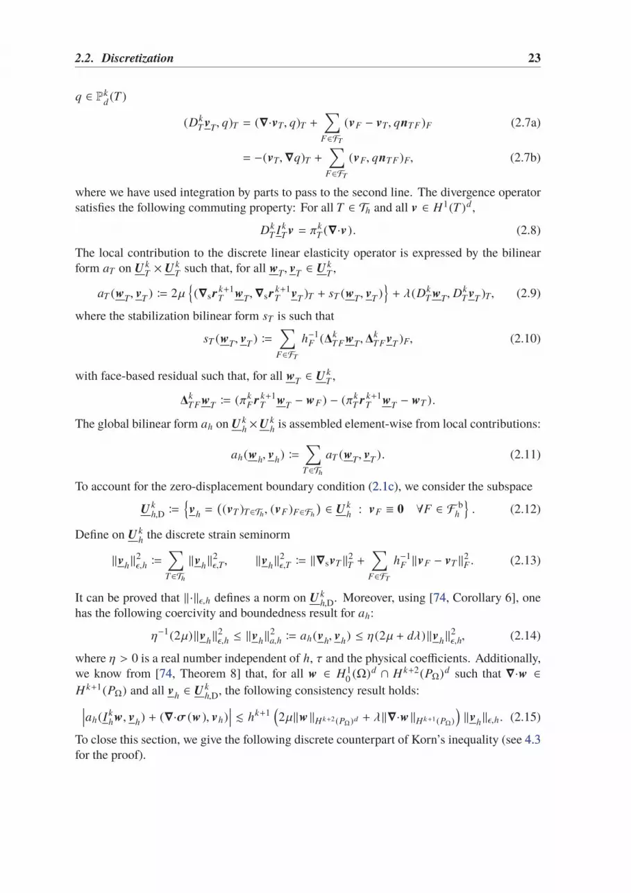
2.2. Discretization 23
q ∈ Pkd(T )
(DkT vT
, q)T = (∇·vT, q)T +
∑
F∈FT(vF − vT, qnTF )F (2.7a)
= −(vT,∇q)T +
∑
F∈FT(vF, qnTF )F, (2.7b)
where we have used integration by parts to pass to the second line. The divergence operatorsatisfies the following commuting property: For all T ∈ Th and all v ∈ H1(T )d ,
DkT I k
T v = πkT (∇·v ). (2.8)
The local contribution to the discrete linear elasticity operator is expressed by the bilinearform aT on U k
T× U k
Tsuch that, for all w
T, v
T∈ U k
T,
aT (wT, v
T) ≔ 2µ
(∇sr
k+1T w
T,∇sr
k+1T v
T)T + sT (w
T, v
T)+ λ(Dk
TwT, Dk
T vT)T, (2.9)
where the stabilization bilinear form sT is such that
sT (wT, v
T) ≔
∑
F∈FTh−1
F (∆kTFwT
,∆kTFvT
)F, (2.10)
with face-based residual such that, for all wT∈ U k
T,
∆kTFwT
≔ (πkF r
k+1T w
T− wF ) − (πk
T rk+1T w
T− wT ).
The global bilinear form ah on U kh×U k
his assembled element-wise from local contributions:
ah(wh, v
h) ≔
∑
T∈ThaT (w
T, v
T). (2.11)
To account for the zero-displacement boundary condition (2.1c2.1c), we consider the subspace
U kh,D ≔
v
h=
(
(vT )T∈Th, (vF )F∈Fh) ∈ U k
h: vF ≡ 0 ∀F ∈ F b
h
. (2.12)
Define on U kh
the discrete strain seminorm
‖vh‖2ǫ,h ≔
∑
T∈Th‖v
h‖2ǫ,T, ‖v
h‖2ǫ,T ≔ ‖∇svT ‖2
T +
∑
F∈FTh−1
F ‖vF − vT ‖2F . (2.13)
It can be proved that ‖·‖ǫ,h defines a norm on U kh,D. Moreover, using [7474, Corollary 6], one
has the following coercivity and boundedness result for ah:
η−1(2µ)‖vh‖2ǫ,h ≤ ‖v
h‖2
a,h ≔ ah(vh, v
h) ≤ η(2µ + dλ)‖v
h‖2ǫ,h, (2.14)
where η > 0 is a real number independent of h, τ and the physical coefficients. Additionally,we know from [7474, Theorem 8] that, for all w ∈ H1
0 (Ω)d ∩ H k+2(PΩ)d such that ∇·w ∈H k+1(PΩ) and all v
h∈ U k
h,D, the following consistency result holds:
ah(I khw, vh
) + (∇·σ (w ), vh) . hk+1
(
2µ‖w ‖Hk+2(PΩ)d + λ‖∇·w ‖Hk+1(PΩ)
)
‖vh‖ǫ,h. (2.15)
To close this section, we give the following discrete counterpart of Korn’s inequality (see 4.34.3for the proof).

24 Chapter 2. The Biot problem
Proposition 2.2 (Discrete Korn’s inequality). There is a real number CK > 0 depending on
and on k but independent of h such that, for all vh∈ U k
h,D, recalling that vh ∈ Pkd(Th)d
denotes the broken polynomial function such that vh |T = vT for all T ∈ Th,
‖vh‖ ≤ CKdΩ‖vh‖ǫ,h, (2.16)
where dΩ denotes the diameter of Ω.
2.2.3 Darcy operator
The discretization of the Darcy operator is based on the Symmetric Weighted Interior Penaltymethod of [7777], cf. also [7676, Section 4.5]. At each time step, the discrete pore pressure issought in the broken polynomial space
Pkh ≔
P
kd(Th) if c0 > 0,
Pkd,0(Th) if c0 = 0,
(2.17)
where we have introduced the zero-average subspacePkd,0(Th) ≔
qh ∈ Pk
d(Th) : (qh, 1) = 0
.
For all F ∈ F ih, we define the jump and (weighted) average operators such that, for all
ϕ ∈ H1(Th), denoting by ϕT and κT the restrictions of ϕ and κ to T ∈ Th, respectively,
[ϕ]F ≔ ϕT1 − ϕT2, ϕF ≔ ωT1ϕT1 + ωT2ϕT2, (2.18)
whereωT1 = 1−ωT2 ≔κT2
(κT1+κT2 ). Denoting by∇h the broken gradient on H1(Th) and letting,
for all F ∈ F ih, λκ,F ≔
2κT1κT2(κT1+κT2 )
, we define the bilinear form ch on Pkh× Pk
hsuch that, for all
qh, rh ∈ Pkh,
ch(rh, qh) ≔ (κ∇hrh,∇hqh) +∑
F∈F ih
ςλκ,F
hF
([rh]F, [qh]F )F
−∑
F∈F ih
(
(κ∇hrhF · nF, [qh]F )F + ([rh]F, κ∇hqhF · nF )F
)
,(2.19)
where ς > 0 is a user-defined penalty parameter. The fact that the boundary terms onlyappear on internal faces in (2.192.19) reflects the Neumann boundary condition (2.1d2.1d). Fromthis point on, we will assume that ς > C2
trN∂ with Ctr denoting the constant from the discretetrace inequality [7676, Eq. (1.37)], which ensures that the bilinear form ch is coercive (in thenumerical tests of Section 2.62.6, we took ς = (N∂ + 0.1)k2). Since the bilinear form ch is alsosymmetric, it defines a seminorm on Pk
h, denoted hereafter by ‖·‖c,h (the map ‖·‖c,h is in fact
a norm on Pkd,0(Th)).
Remark 2.3 (Alternative stabilization). To get rid of the dependence of the lower thresholdof ς on Ctr, one can resort to the BR2 stabilization; c.f. [1717] and also [7676, Section 5.3.2]. Inpassing, this stabilization could also contribute to handle face degeneration since the penaltyparameter no longer depends on the inverse of the face diameter (cf. Remark 2.12.1). This topicwill make the object of future investigations.

2.2. Discretization 25
The following known results will be needed in the analysis. Let
P∗ ≔r ∈ H1(Ω) ∩ H2(PΩ) : κ∇r · n = 0 on ∂Ω
, Pk
∗h ≔ P∗ + Pkh .
Extending the bilinear form ch to Pk∗h× Pk
∗h, the following consistency result can be proved
adapting the arguments of [7676, Chapter 4] to account for the homogeneous Neumann boundarycondition (2.1d2.1d):
∀r ∈ P∗, −(∇·(κ∇r), q) = ch(r, q) ∀q ∈ P∗h. (2.20)
Assuming, additionally, that r ∈ H k+2(PΩ), as a consequence of [7676, Lemma 5.52] togetherwith the optimal approximation properties (2.22.2) of πk
hon regular mesh sequences one has,
supqh∈Pkd,0(Th )\0
ch(r − πkhr, qh)
‖qh‖c,h. κ
1/2hk ‖r ‖Hk+1(PΩ) .
2.2.4 Hydro-mechanical coupling
The hydro-mechanical coupling is realized by means of the bilinear form bh on U kh× Pk
d(Th)
such that, for all vh∈ U k
hand all qh ∈ Pk
d(Th),
bh(vh, qh) ≔
∑
T∈ThbT (v
T, qh |T ), bT (v
T, qh |T ) ≔ −(Dk
T vT, qh |T )T, (2.21)
where DkT
is the discrete divergence operator defined by (2.7a2.7a). A simple verification showsthat, for all v
h∈ U k
hand all qh ∈ Pk
d(Th),
bh(vh, qh) . ‖v
h‖ǫ,h‖qh‖. (2.22)
Additionally, using the definition (2.7a2.7a) of DkT
and (2.122.12) of U kh,D, it can be proved that, for
all vh∈ U k
h,D, it holds (χΩ denotes here the characteristic function of Ω),
bh(vh, χΩ) = 0. (2.23)
The following inf-sup condition expresses the stability of the hydro-mechanical coupling:Lemma 2.4 (Inf-sup condition for bh). There is a real number β depending on Ω, and k
but independent of h such that, for all qh ∈ Pkd,0(Th),
‖qh‖ ≤ β supvh∈Uk
h,D\0
bh(vh, qh)
‖vh‖ǫ,h
. (2.24)
Proof. Let qh ∈ Pkd,0(Th). Classically [3131], there is vqh ∈ H1
0 (Ω)d such that ∇·vqh = qh and
‖vqh ‖H1(Ω)d . ‖qh‖. Let T ∈ Th. Using the H1-stability of the L2-orthogonal projector (cf.,e.g., [6969, Corollary 3.7]), it is inferred that
‖∇sπkT vqh ‖T ≤ ‖∇vqh ‖T .
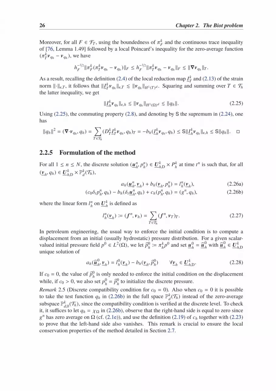
26 Chapter 2. The Biot problem
Moreover, for all F ∈ FT , using the boundedness of πkF
and the continuous trace inequalityof [7676, Lemma 1.49] followed by a local Poincaré’s inequality for the zero-average function(πk
Tvqh − vqh ), we have
h−1/2F
‖πkF (πk
T vqh − vqh )‖F ≤ h−1/2F
‖πkT vqh − vqh ‖F . ‖∇vqh ‖T .
As a result, recalling the definition (2.42.4) of the local reduction map I kT
and (2.132.13) of the strainnorm ‖·‖ǫ,T , it follows that ‖I k
Tvqh ‖ǫ,T . ‖vqh ‖H1(T )d . Squaring and summing over T ∈ Th
the latter inequality, we get
‖I khvqh ‖ǫ,h . ‖vqh ‖H1(Ω)d . ‖qh‖. (2.25)
Using (2.252.25), the commuting property (2.82.8), and denoting by S the supremum in (2.242.24), onehas
‖qh‖2= (∇·vqh, qh) =
∑
T∈Th(Dk
T I kT vqh, qh)T = −bh(I k
hvqh, qh) ≤ S‖I khvqh ‖ǫ,h . S‖qh‖.
2.2.5 Formulation of the method
For all 1 ≤ n ≤ N , the discrete solution (unh, pn
h) ∈ U k
h,D × Pkh
at time tn is such that, for all
(vh, qh) ∈ U k
h,D × Pkd(Th),
ah(unh, vh
) + bh(vh, pn
h) = lnh(v
h), (2.26a)
(c0δt pnh, qh) − bh(δtu
nh, qh) + ch(pn
h, qh) = (gn, qh), (2.26b)
where the linear form lnh
on U kh
is defined as
lnh(v
h) ≔ ( f n, vh) =
∑
T∈Th( f n, vT )T . (2.27)
In petroleum engineering, the usual way to enforce the initial condition is to compute adisplacement from an initial (usually hydrostatic) pressure distribution. For a given scalar-valued initial pressure field p0 ∈ L2(Ω), we let p0
h≔ πk
hp0 and set u0
h= u
0h with u
0h ∈ U k
h,Dunique solution of
ah(u0h, vh
) = l0h(v
h) − bh(v
h, p0
h) ∀vh∈ U k
h,D. (2.28)
If c0 = 0, the value of p0h
is only needed to enforce the initial condition on the displacementwhile, if c0 > 0, we also set p0
h= p0
hto initialize the discrete pressure.
Remark 2.5 (Discrete compatibility condition for c0 = 0). Also when c0 = 0 it is possibleto take the test function qh in (2.26b2.26b) in the full space Pk
d(Th) instead of the zero-average
subspace Pkd,0(Th), since the compatibility condition is verified at the discrete level. To check
it, it suffices to let qh = χΩ in (2.26b2.26b), observe that the right-hand side is equal to zero sinceg
n has zero average on Ω (cf. (2.1e2.1e)), and use the definition (2.192.19) of ch together with (2.232.23)to prove that the left-hand side also vanishes. This remark is crucial to ensure the localconservation properties of the method detailed in Section 2.72.7.

2.3. Stability analysis 27
2.3 Stability analysis
In this section we study the stability of problem (2.262.26) and prove its well-posedness. We recallthe following discrete Gronwall’s inequality, which is a minor variation of [121121, Lemma 5.1].Lemma 2.6 (Discrete Gronwall’s inequality). Let an integer N and reals δ,G > 0, and K ≥ 0be given, and let (an)0≤n≤N , (bn)0≤n≤N , and (γn)0≤n≤N denote three sequences of nonnegative
real numbers such that, for all 0 ≤ n ≤ N
an+ δ
n∑
m=0
bm+ K ≤ δ
n∑
m=0
γmam+ G.
Then, if γmδ < 1 for all 0 ≤ m ≤ N , letting ςm≔ (1 − γmδ)−1, it holds, for all 0 ≤ n ≤ N ,
an+ δ
n∑
m=0
bm+ K ≤ exp *,δ
n∑
m=0
ςmγm+- × G. (2.29)
Lemma 2.7 (A priori bounds). Assume f ∈ C1(L2(Ω)d) and g ∈ C0(L2(Ω)), and let
(u0h, p0
h) = (u
0h, p0
h) with (u
0h, p0
h) defined as in Section 2.2.52.2.5. For all 1 ≤ n ≤ N , denote by
(unh, pn
h) the solution to (2.262.26). Then, for τ small enough, it holds that
‖uNh ‖
2a,h + ‖c
1/20 pN
h ‖2+
1
2µ + dλ‖pN
h − pNh ‖2+
N∑
n=1
τ‖pnh‖
2c,h .
(
1
2µ+ c0
)
‖p0‖2+
d2Ω
2µ‖ f ‖2
C1(L2(Ω)d )+ (2µ + dλ)t2
F‖g‖2C0(L2(Ω))
+
t2F
c0‖g‖2
C0(L2(Ω)), (2.30)
with the convention that c−10 ‖g‖2
C0(L2(Ω))= 0 if c0 = 0 and, for 0 ≤ n ≤ N , pn
h ≔ (pnh, 1).
Remark 2.8 (Well-posedness). Owing to linearity, the well-posedness of (2.262.26) is an imme-diate consequence of Lemma 2.72.7.
Remark 2.9 (A priori bound for c0 = 0). When c0 = 0, the choice (2.172.17) of the discrete spacefor the pressure ensures that pn
h = 0 for all 0 ≤ n ≤ N . Thus, the third term in the left-handside of (2.302.30) yields an estimate on ‖pN
h‖2, and the a priori bound reads
‖uNh ‖
2a,h +
1
2µ + dλ‖pN
h ‖2+
N∑
n=1
τ‖pnh‖
2c,h .
(2µ)−1(
d2Ω‖ f ‖2
C1(L2(Ω)d )+ ‖p0‖2
)
+ (2µ + dλ)t2F‖g‖2
C0(L2(Ω)).
The convention c−10 ‖g‖2
C0(L2(Ω))= 0 if c0 = 0 is justified since the term T2 in point (4) of the
following proof vanishes in this case thanks to the compatibility condition (2.1e2.1e).
Proof of Lemma 2.72.7. Throughout the proof, Ci with i ∈ N∗ will denote a generic positiveconstant independent of h, τ, and of the physical parameters c0, λ, µ, and κ .

28 Chapter 2. The Biot problem
(1) Estimate of ‖pnh− pn
h‖. Using the inf-sup condition (2.242.24) followed by (2.232.23) to inferthat bh(v
h, pn
h) = 0, the mechanical equilibrium equation (2.26a2.26a), and the second inequalityin (2.142.14), for all 1 ≤ n ≤ N we get
‖pnh − pn
h‖ ≤ β supvh∈Uk
h,D\0
bh(vh, pn
h− pn
h)
‖vh‖ǫ,h
= β supvh∈Uk
h,D\0
bh(vh, pn
h)
‖vh‖ǫ,h
= β supvh∈Uk
h,D\0
lnh(v
h) − ah(un
h, v
h)
‖vh‖ǫ,h
≤ C1/21
(
dΩ‖ f n‖ + (2µ + dλ)1/2‖un
h‖a,h
)
,
where we have set, for the sake of brevity, C1/21 ≔ βmax(CK, η). This implies, in particular,
‖pnh − pn
h‖2 ≤ 2C1
(
d2Ω‖ f
n‖2+ (2µ + dλ)‖un
h‖2a,h
)
(2.31)
(2) Energy balance. Adding (2.26a2.26a) with vh= τδtu
nh
to (2.26b2.26b) with qh = τpnh, and summing
the resulting equation over 1 ≤ n ≤ N , it is inferred
N∑
n=1
τah(unh, δtu
nh)+
N∑
n=1
τ(c0δt pnh, pn
h)+
N∑
n=1
τ‖pnh‖
2c,h =
N∑
n=1
τlnh(δtu
nh)+
N∑
n=1
τ(gn, pnh). (2.32)
We denote by L and R the left- and right-hand side of (2.322.32) and proceed to find suitablelower and upper bounds, respectively.(3) Lower bound for L. Using twice the formula
2x(x − y) = x2+ (x − y)2 − y
2, (2.33)
and telescoping out the appropriate summands, the first two terms in the left-hand sideof (2.322.32) can be rewritten as, respectively,
N∑
n=1
τah(unh, δtu
nh) =
1
2‖uN
h ‖2a,h +
1
2
N∑
n=1
τ2‖δtunh‖
2a,h −
1
2‖u0
h‖2a,h,
N∑
n=1
τ(c0δt pnh, pn
h) =1
2‖c1/2
0 pNh ‖
2+
1
2
N∑
n=1
τ2‖c1/20 δt p
nh‖
2 − 1
2‖c1/2
0 p0h‖
2.
Using the above relation together with (2.312.31) and ‖ f N ‖ ≤ ‖ f ‖C1(L2(Ω)d ), it is inferred that
1
4‖uN
h ‖2a,h −
1
2‖u0
h‖2a,h +
1
2‖c1/2
0 pNh ‖
2 − 1
2‖c1/2
0 p0h‖
2
+
1
8C1(2µ + dλ)‖pN
h − pNh ‖2+
N∑
n=1
τ‖pnh‖
2c,h ≤ L +
d2Ω
4(2µ + dλ)‖ f ‖2
C1(L2(Ω)d ). (2.34)

2.3. Stability analysis 29
(4) Upper bound for R. For the first term in the right-hand side of (2.322.32), discrete integrationby parts in time yields
N∑
n=1
τlnh(δtu
nh) = ( f N, uN
h ) − ( f 0, u0h) −
N∑
n=1
τ(δt fn, un−1
h ),
hence, using the Cauchy–Schwarz inequality, the discrete Korn’s inequality followed by (2.142.14)
to estimate ‖unh‖2 ≤ C2d2
Ω
µ ‖unh‖2
a,hfor all 1 ≤ n ≤ N (with C2 ≔ C2
Kη/2), and Young’sinequality, one has
N
∑
n=1
τlnh(δtu
nh)
≤1
8*,‖u
Nh ‖
2a,h + ‖u
0h‖
2a,h +
1
2tF
N∑
n=1
τ‖un−1h ‖2
a,h+-
+
C2d2Ω
µ*,‖ f
N ‖2+ ‖ f 0‖2
+ 2tF
N∑
n=1
τ‖δt fn‖2+-
≤ 1
8*,‖u
Nh ‖
2a,h + ‖u
0h‖
2a,h +
1
2tF
N∑
n=0
τ‖unh‖
2a,h+- +
C2C3d2Ω
µ‖ f ‖2
C1(L2(Ω)d ),
(2.35)where we have used the classical bound ‖ f N ‖2
+‖ f 0‖2+2tF
∑Nn=1 τ‖δt f
n‖2 ≤ C3‖ f ‖2C1(L2(Ω)d )
to conclude. We proceed to estimate the second term in the right-hand side of (2.322.32) by split-ting it into two contributions as follows (here, gn
≔ (gn, 1)):
N∑
n=1
τ(gn, pnh) =
N∑
n=1
τ(gn, pnh − pn
h) +
N∑
n=1
τ(gn, pn
h) ≔ T1 + T2.
Using the Cauchy–Schwarz inequality, the bound∑N
n=1 τ‖gn‖2 ≤ tF‖g‖2C0(L2(Ω))
togetherwith (2.312.31) and Young’s inequality, it is inferred that
|T1 | ≤
N∑
n=1
τ‖gn‖2
1/2
×
N∑
n=1
τ‖pnh − pn
h‖2
1/2
≤ tF‖g‖C0(L2(Ω)) ×
2C1
tF
N∑
n=1
τ(
d2Ω‖ f
n‖2+ (2µ + dλ)‖un
h‖2a,h
)1/2
≤ 8C1t2F(2µ + dλ)‖g‖2
C0(L2(Ω))+
d2Ω
16(2µ + dλ)‖ f ‖2
C1(L2(Ω)d )+
1
16tF
N∑
n=1
τ‖unh‖
2a,h.
(2.36)Owing the compatibility condition (2.1e2.1e), T2 = 0 if c0 = 0. If c0 > 0, using the Cauchy–

30 Chapter 2. The Biot problem
Schwarz and Young’s inequalities, we have
|T2 | ≤tF
N∑
n=1
τc−10 ‖gn‖2
1/2
×t−1
F
N∑
n=1
τ‖c1/20 pn
h‖2
1/2
≤t2F
2c0‖g‖2
C0(L2(Ω))+
1
2tF
N∑
n=1
τ‖c1/20 pn
h‖2.
(2.37)
Using (2.352.35), (2.362.36), and (2.372.37), we infer
R ≤ 1
8*,‖u
Nh ‖
2a,h + t−1
F
N∑
n=0
τ‖unh‖
2a,h + ‖u
0h‖
2a,h+- +
1
2tF
N∑
n=1
τ‖c1/20 pn
h‖2+
t2F
2c0‖g‖2
C0(L2(Ω))
+ 8C1t2F(2µ + dλ)‖g‖2
C0(L2(Ω))+
(
1
16(2µ + dλ)+
C2C3
µ
)
d2Ω‖ f ‖2
C1(L2(Ω)d ). (2.38)
(5) Conclusion. Using (2.342.34), the fact that L = R owing to (2.322.32), and (2.382.38), it is inferredthat
‖uNh ‖
2a,h + 4‖c1/2
0 pNh ‖
2+
1
(2µ + dλ)‖pN
h − pNh ‖2+ 8
N∑
n=1
τ‖pnh‖
2c,h ≤
C4
tF
N∑
n=0
τ‖unh‖
2a,h +
C4
tF
N∑
n=1
τ4‖c1/20 pn
h‖2+ G,
where C4 ≔ max(1,C1) while, observing that ‖c1/20 p0
h‖ ≤ ‖c1/2
0 p0‖ since πkh
is a bounded
operator, and that it follows from (2.392.39) below that ‖u0h‖2
a,h≤ C5(2µ)−1
(
d2Ω‖ f 0‖2
+ ‖p0‖2)
,
C−14 G ≔
5C5
2µ
(
d2Ω‖ f
0‖2+ ‖p0‖2
)
+ 4‖c1/20 p0‖2
+
4t2F
c0‖g‖2
C0(L2(Ω))
+ 64C1t2F(2µ + dλ)‖g‖2
C0(L2(Ω))+
(
5
2(2µ + dλ)+
8C2C3
µ
)
d2Ω‖ f ‖2
C1(L2(Ω)d ).
Using Gronwall’s Lemma 2.62.6 with a0≔ ‖u0
h‖2
a,hand an
≔ ‖unh‖2
a,h+ 4‖c1/2
0 pnh‖2 for 1 ≤ n ≤
N , δ ≔ τ, b0≔ 0 and bn
≔ ‖pnh‖2
c,hfor 1 ≤ n ≤ N , K = 1
(2µ+dλ)‖pN
h− pN
h ‖2, and γn=
C4tF
,the desired result follows.
Proposition 2.10 (Stability and approximation properties for u0h). The initial displace-
ment (2.282.28) satisfies the following stability condition:
‖ u0h‖a,h . (2µ)−
1/2(
dΩ‖ f 0‖ + ‖p0‖)
. (2.39)
Additionally, recalling the global reduction map I kh
defined by (2.42.4), and assuming the
additional regularity p0 ∈ H k+1(PΩ), u0 ∈ H k+2(PΩ)d , and ∇·u0 ∈ H k+1(PΩ), it holds
(2µ)1/2‖ u0
h − I khu
0‖a,h . hk+1(
2µ‖u0‖Hk+2(PΩ)d + λ‖∇·u0‖Hk+1(PΩ) + ρ1/2κ ‖p0‖Hk+1(PΩ)
)
,(2.40)
with global heterogeneity ratio ρκ ≔ κ/κ.

2.4. Error analysis 31
Proof. (1) Proof of (2.392.39). Using the first inequality in (2.142.14) followed by the definition (2.282.28)of u0
h, we have
‖ u0h‖a,h . sup
vh∈Ukh,D\0
ah(u0h, vh
)
(2µ)1/2‖vh‖ǫ,h
= (2µ)−1/2 sup
vh∈Ukh,D\0
l0h(v
h) − bh(v
h, πk
hp0)
‖vh‖ǫ,h
. (2µ)−1/2
(
dΩ‖ f 0‖ + ‖p0‖)
,
where to conclude we have used the Cauchy–Schwarz and discrete Korn’s (2.162.16) inequalitiesfor the first term in the numerator and the continuity (2.222.22) of bh together with the L2(Ω)-stability of πk
hfor the second. (2) Proof of (2.402.40). The proof is analogous to that of point (3)
in Lemma 2.112.11 except that we use the approximation properties (2.22.2) of πkh
instead of (2.452.45).For this reason, elliptic regularity is not needed.
2.4 Error analysis
In this section we carry out the error analysis of the method.
2.4.1 Projection
We consider the error with respect to the sequence of projections (unh, pn
h)1≤n≤N , of the exact
solution defined as follows: For 1 ≤ n ≤ N , pnh∈ Pk
hsolves
ch(pnh, qh) = ch(pn, qh) ∀qh ∈ Pk
d (Th), (2.41a)
with the closure condition∫
Ωpn
h=
∫
Ωpn. Once pn
hhas been computed, un
h ∈ U kh,D solves
ah(unh, vh
) = lnh(v
h) − bh(v
h, pn
h) ∀vh∈ U k
h,D. (2.41b)
The well-posedness of problems (2.41a2.41a) and (2.41b2.41b) follow, respectively, from the coercivityof ch on Pk
d,0(Th) and of ah on U kh,D. The projection (u
nh, pn
h) is chosen so that a convergence
rate of (k+1) in space analogous to the one derived in [7474] can be proved for the ‖·‖a,h-norm ofthe displacement at final time tF. To this purpose, we also need in what follows the followingelliptic regularity, which holds, e.g., when Ω is convex: There is a real number Cell > 0 onlydepending on Ω such that, for all ψ ∈ L2
0(Ω), with L20(Ω) ≔
q ∈ L2(Ω) : (q, 1) = 0
, the
unique function ζ ∈ H1(Ω) ∩ L20(Ω) solution of the homogeneous Neumann problem
−∇·(κ∇ζ ) = ψ in Ω, κ∇ζ · n = 0 on ∂Ω, (2.42)
is such that‖ζ ‖H2(PΩ) ≤ Cellκ
−1/2‖ψ‖. (2.43)
For further insight on the role of the choice (2.412.41) and of the elliptic regularity assumptionwe refer to Remark 2.142.14.

32 Chapter 2. The Biot problem
Lemma 2.11 (Approximation properties for (unh, pn
h)). Let a time step 1 ≤ n ≤ N be fixed.
Assuming the regularity pn ∈ H k+1(PΩ), it holds
‖ pnh − pn‖c,h . hk κ
1/2‖pn‖Hk+1(PΩ) . (2.44)
Moreover, recalling the global reduction map I kh
defined by (2.42.4), further assuming the reg-
ularity un ∈ H k+2(PΩ)d , ∇·un ∈ H k+1(PΩ), and provided that the elliptic regularity (2.432.43)holds, one has
‖ pnh − pn‖ . hk+1ρ
1/2κ ‖pn‖Hk+1(PΩ), (2.45)
(2µ)1/2‖ un
h − I khu
n‖a,h . hk+1(
2µ‖un‖Hk+2(PΩ)d + λ‖∇·un‖Hk+1(PΩ) + ρ1/2κ ‖pn‖Hk+1(PΩ)
)
.
(2.46)
Proof. (1) Proof of (2.442.44). By definition, we have that ‖ pnh−pn‖c,h = infqh∈Pkd (Th ) ‖qh−pn‖c,h.
To prove (2.442.44), it suffices to take qh = πkh
pn in the right-hand side of the previous expressionand use the approximation properties (2.22.2) of πk
h.
(2) Proof of (2.452.45). Let ζ ∈ H1(Ω) solve (2.422.42) with ψ = pn − pnh. From the consistency
property (2.202.20), it follows that
‖ pnh − pn‖2
= −(∇·(κ∇ζ ), pnh − pn) = ch(ζ, pn
h − pn) = ch(ζ − π1hζ, pn
h − pn).
Then, using the Cauchy–Schwarz inequality, the estimate (2.442.44) together with the approxi-mation properties (2.22.2) of π1
h, and elliptic regularity, it is inferred that
‖ pnh − pn‖2
= ch(ζ − π1hζ, pn
h − pn) ≤ ‖ζ − π1hζ ‖c,h‖ pn
h − pn‖c,h
. hk+1κ1/2‖ζ ‖H2(PΩ) ‖pn‖Hk+1(PΩ) . hk+1ρ
1/2κ ‖ pn
h − pn‖‖pn‖Hk+1(PΩ),
and (2.452.45) follows.(3) Proof of (2.462.46). We start by observing that
‖ unh − I k
hun‖a,h = sup
vh∈Ukh\0
ah(unh − I k
hun, v
h)
‖vh‖a,h
. supvh∈Uk
h\0
ah(unh − I k
hun, v
h)
(2µ)1/2‖vh‖ǫ,h
,
where we have used the first inequality in (2.142.14). Recalling the definition (2.272.27) of the linearform ln
h, the fact that f n
= −∇·σ (u ) + ∇p, and using (2.41a2.41a), it is inferred that
ah(unh − I k
hun, v
h) = ln
h(vnh) − ah(I k
hun, v
h) − bh(v
h, phn)
=
− ah(I khu
n, vh) − (∇·σ (un), vh)
+
(∇pn, vh) − bh(vh, pn
h)
.(2.47)
Denote by T1 and T2 the terms in braces. Using (2.152.15), it is readily inferred that
|T1 | . hk+1(
2µ‖un‖Hk+2(PΩ)d + λ‖∇·un‖Hk+1(PΩ)
)
‖vh‖ǫ,h. (2.48)

2.4. Error analysis 33
For the second term, performing an element-wise integration by parts on (∇p, vh) andrecalling the definition (2.212.21) of bh and (2.7a2.7a) of Dk
Twith q = pn
h, it is inferred that
|T2 | =∑
T∈Th
(pnh − pn,∇·vT )T +
∑
F∈FT(pn
h − pn, (vF − vT )nTF )F
. hk+1ρ1/2κ ‖pn‖Hk+1(PΩ) ‖vh
‖ǫ,h,
(2.49)
where the conclusion follows from the Cauchy–Schwarz inequality together with (2.452.45).Plugging (2.482.48)–(2.492.49) into (2.472.47) we obtain (2.462.46).
2.4.2 Error equations
We define the discrete error components as follows: For all 1 ≤ n ≤ N ,
enh≔ un
h − unh, ρn
h ≔ pnh − pn
h. (2.50)
Owing to the choice of the initial condition detailed in Section 2.2.52.2.5, the inital error (e0h, ρ0
h) ≔
(u0h− u
0h, p0
h− p0
h) is the null element in the product space U k
h,D × Pkh. On the other hand, for
all 1 ≤ n ≤ N , (enh, ρn
h) solves
ah(enh, v
h) + bh(v
h, ρn
h) = 0 ∀vh∈ U k
h, (2.51a)
(c0δt ρnh, qh) − bh(δt e
nh, qh) + ch(ρn
h, qh) = Enh (qh), ∀qh ∈ Pk
h, (2.51b)
with consistency error
Enh (qh) ≔ (gn, qh) − (c0δt p
nh, qh) − ch(pn
h, qh) + bh(δt unh, qh).
2.4.3 Convergence
Theorem 2.12 (Estimate for the discrete errors). Let (u, p) denote the unique solution to (2.12.1),for which we assume the regularity
u ∈ C2(H1(PΩ)d) ∩ C1(H k+2(PΩ)d), p ∈ C1(H k+1(PΩ)).
If c0 > 0, we further assume p ∈ C2(L2(Ω)). Define, for the sake of brevity, the bounded
quantities
N1 ≔(
2µ + dλ)1/2 ‖u ‖C2(H1(PΩ)d ) + ‖c
1/20 p‖C2(L2(Ω)d ),
N2 ≔(2µ + dλ)
1/2
2µ
(
2µ‖u ‖C1(Hk+2(PΩ)d ) + λ‖∇·u ‖C1(Hk+1(PΩ)) + ρ1/2κ ‖p‖C1(Hk+1(PΩ))
)
+ ‖c1/20 p‖C0(Hk+1(PΩ)) .
Then, assuming the elliptic regularity (2.432.43), it holds, letting ρnh ≔ (ρn
h, 1),
‖eNh‖2
a,h + ‖c1/20 ρN
h ‖2+
1
2µ + dλ‖ρN
h − ρNh ‖2+
N∑
n=1
τ‖ρnh‖
2c,h .
(
τN1 + hk+1N2
)2. (2.52)

34 Chapter 2. The Biot problem
Remark 2.13 (Pressure estimate for c0 = 0). In the incompressible case c0 = 0, the thirdterm in the left-hand side of (2.522.52) delivers an estimate on the L2-norm of the pressure sinceρN
h = 0 (cf. (2.1f2.1f)).
Proof of Theorem 2.122.12. Throughout the proof, Ci with i ∈ N∗ will denote a generic positiveconstant independent of h, τ, and of the physical parameters c0, λ, µ, and κ .(1) Basic error estimate. Using the inf-sup condition (2.242.24), equation (2.232.23) followedby (2.51a2.51a), and the second inequality in (2.142.14), it is readily seen that
‖ρnh − ρn
h‖ ≤ β supvh∈Uk
h,D\0
bh(vh, ρn
h− ρn
h)
‖vh‖ǫ,h
= β supvh∈Uk
h,D\0
−ah(enh, v
h)
‖vh‖ǫ,h
≤ C1/21 (2µ + dλ)
1/2‖enh‖a,h,
with C1/21 = βη
1/2. Adding (2.51a2.51a) with vh= τδt eh
to (2.51b2.51b) with qh = τρnh
and summingthe resulting equation over 1 ≤ n ≤ N , it is inferred that
N∑
n=1
τah(enh, δt e
nh) +
N∑
n=1
τ(c0δt ρnh, ρ
nh) +
N∑
n=1
τ‖ρnh‖
2c,h =
N∑
n=1
τEnh (ρn
h). (2.53)
Proceeding as in point (3) of the proof of Lemma 2.72.7, and recalling that (e0h, ρ0
h) = (0, 0), we
arrive at the following error estimate:
1
4‖eN
h‖2
a,h +1
4C1(2µ + dλ)‖ρN
h − ρNh ‖2+
1
2‖c1/2
0 ρNh ‖
2+
N∑
n=1
τ‖ρnh‖
2c,h ≤
N∑
n=1
τEnh (ρn
h). (2.54)
(2) Bound of the consistency error. Using gn= c0dt p
n+ ∇·(dtu
n − κ∇pn), the consistencyproperty (2.202.20), and observing that, using the definition (2.192.19) of ch, integration by partstogether with the homogeneous displacement boundary condition (2.1c2.1c), and (2.232.23),
ch(pn − pnh, ρ
nh) + (∇·(dtu
n), ρnh) + bh(δt u
nh, ρ
nh) = 0,
we can decompose the right-hand side of (2.542.54) as follows:
N∑
n=1
τEnh (ρn
h) =
N∑
n=1
τ(c0(dt pn − δt p
nh), ρn
h) +
N∑
n=1
τch(pn − pnh, ρ
nh − ρn
h)
+
N∑
n=1
τ(∇·(dtu
n), ρnh − ρn
h) + bh(δt unh, ρ
nh − ρn
h)≔ T1 + T2 + T3.
(2.55)For the first term, inserting±δt p
n into the first factor and using the Cauchy-Schwarz inequalityfollowed by the approximation properties of p0
h(a consequence of (2.22.2)) and (2.452.45) of pn
h, it

2.4. Error analysis 35
is inferred that
|T1 | .c0
N∑
n=1
τ[‖dt p
n − δt pn‖2+ ‖δt (pn − pn
h)‖2]
1/2
×
N∑
n=1
τ‖c1/20 ρn
h‖2
1/2
≤ C2
(
τN1 + hk+1N2
)
+
1
2
N∑
n=1
τ‖c1/20 ρn
h‖2.
(2.56)
For the second term, the choice (2.41a2.41a) of the pressure projection readily yields
T2 = 0.
For the last term, inserting ±I khun into the first argument of bh, and using the commuting
property (2.82.8) of DkT, it is inferred that
T3 =
N∑
n=1
τ
∑
T∈Th
[(∇·(dtu
n − δtun), ρn
h − ρnh)T + (Dk
Tδt (I kTu
n − unT ), ρn
h − ρnh)T
] .Using the Cauchy–Schwarz inequality, the bound ‖Dk
Tδt (I k
Tun− u
nT )‖T . ‖δt (I k
Tun− u
nT )‖ǫ,T
valid for all T ∈ Th, and the approximation properties (2.402.40) and (2.462.46) of u0h and u
nh,
respectively, we obtain
|T3 | .
N∑
n=1
τ[‖dtu
n − δtun‖2
H1(Ω)d+ ‖δt (I k
hun − u
nh)‖2
ǫ,h
]12
×
N∑
n=1
τ‖ρnh − ρn
h‖2
12
≤ C3C1
(
τN1 + hk+1N2
)2+
1
4C1(2µ + dλ)
N∑
n=1
τ‖ρnh − ρn
h‖2.
(2.57)Using (2.562.56)–(2.572.57) to bound the right-hand side of (2.552.55), it is inferred
‖eNh‖2
a,h +1
C1(2µ + dλ)‖ρN
h − ρNh ‖2+ 2‖c1/2
0 ρNh ‖
2+ 4
N∑
n=1
τ‖ρnh‖
2c,h
≤ 1
C1(2µ + dλ)
N∑
n=1
τ‖ρnh − ρn
h‖2+ 2
N∑
n=1
τ‖c1/20 ρn
h‖2+ G,
with G ≔ 4(C1C3 + C2)(
τN1 + hk+1N2
)2. The conclusion follows using the discrete Gron-
wall’s inequality (2.292.29) with δ = τ, K = ‖eNh‖2
a,h, a0= 0 and an
=1
C1(2µ+dλ)‖ρn
h− ρn
h‖2+
2‖c1/20 ρn
h‖2 for 1 ≤ n ≤ N , bn
= 4‖ρnh‖2
c,h, and γn
= 1.
Remark 2.14 (Role of the choice (2.412.41) and of elliptic regularity). The choice (2.412.41) for theprojection ensures that the term T2 in step (2) of the proof of Theorem 2.122.12 vanishes. This isa key point to obtain an order of convergence of (k + 1) in space. For a different choice, saypn
h= πk
hpn, this term would be of order k, and therefore yield a suboptimal estimate for the
terms in the left-hand side of (2.582.58) below (the estimate (2.592.59) would not change and remainoptimal). This would also be the case if we removed the elliptic regularity assumption (2.432.43).

36 Chapter 2. The Biot problem
Remark 2.15 (BDF2 time discretization). In some of the numerical test cases of Section 2.62.6,we have used a BDF2 time discretization, which corresponds to the backward differencingoperator
δ(2)t ϕn+2
≔3ϕn+2 − 4ϕn+1
+ ϕn
2τ,
used in place of (2.32.3). As BDF2 requires two starting values, we perform a first march intime using the backward Euler scheme (another possibility would have been to resort to thesecond-order Crank–Nicolson scheme). For the BDF2 time discretization, stability estimatessimilar to those of Lemma 2.72.7 can be proved with this initialization, while the error can beshown to scale as τ2
+ hk+1 (compare with (2.522.52)). The main difference with respect to thepresent analysis focused on the backward Euler scheme is that formula (2.332.33) is replaced inthe proofs by
2x(3x − 4y + z) = x2 − y2+ (2x − y)2 − (2y − z)2
+ (x − 2y + z)2.
The modifications of the proofs are quite classical and are not detailed here for the sake ofconciseness (for a pedagogic exposition, one can consult, e.g., [9292, Chapter 6]).
Corollary 2.16 (Convergence). Under the assumptions of Theorem 2.122.12, it holds that
(2µ)1/2‖∇s,h(r k+1
h uNh − uN )‖ + ‖c1/2
0 (pNh − pN )‖ + 1
2µ + dλ‖(pN
h − pN ) − (pNh − pN
)‖
. τN1 + hk+1N2 + c1/20 hk+1‖pN ‖Hk+1(PΩ), (2.58)
N
∑
n=1
τ‖pnh − pn‖2
c,h
1/2
. τN1 + hk+1N2 + hk κ1/2t
1/2F ‖p‖C0(Hk+1(PΩ)) . (2.59)
Proof. Using the triangle inequality, recalling the definition (2.502.50) of eNh
and pNh
and (2.142.14)of ‖·‖a,h-norm, it is inferred that
(2µ)1/2‖∇s,h(r k+1
h uNh − uN )‖ . ‖eN
h‖a,h + (2µ)
1/2‖∇s,h(r k+1h uh − r k+1
h I khu
N )‖+ (2µ)
1/2‖∇s(r k+1h I k
huN − uN )‖,
‖pNh − pN − (pN
h − pN)‖ ≤ ‖ρN
h − ρNh ‖ + ‖ pN
h − pN ‖,‖c1/2
0 (pNh − pN )‖ ≤ ‖c1/2
0 ρNh ‖ + ‖c
1/20 (pN
h − pN )‖.
To conclude, use (2.522.52) to estimate the left-most terms in the right-hand sides of the aboveequations. Use (2.462.46) and (2.452.45), the approximation properties (2.62.6) of r k+1
hI k
h, respec-
tively, for the right-most terms. This proves (2.582.58). A similar decomposition of the erroryields (2.592.59).

2.5. Implementation 37
2.5 Implementation
In this section we discuss practical aspects including, in particular, static condensation. Theimplementation is based on the hho platform11, which relies on the linear algebra facilitiesprovided by the Eigen3 library [116116].
The starting point consists in selecting a basis for each of the polynomial spaces appearingin the construction. Let s = (s1, ..., sd) be a d-dimensional multi-index with the usual notation|s |1 =
∑di=1 si, and let x = (x1, ..., xd) ∈ Rd . Given k ≥ 0 and T ∈ Th, we denote by Bk
Ta
basis for the polynomial space Pkd(T ). In the numerical experiments of Section 2.62.6, we have
used the set of locally scaled monomials:
BkT ≔
(
x − xT
hT
) s
, |s |1 ≤ k
, (2.60)
with xT denoting the barycenter of T . Similarly, for all F ∈ Fh, we denote by BkF
a basisfor the polynomial space Pk
d−1(F) which, in the proposed implementation, is again a set oflocally scaled monomials similar to (2.602.60).
Remark 2.17 (Choice of the polynomial bases). The choice of the polynomial bases can havea sizeable impact on the conditioning of both the local problems defining the displacementreconstruction r k+1
T(cf. (2.52.5)) and the global problem. This is particularly the case when using
high polynomial orders (typically, k ≥ 7). The scaled monomial basis (2.602.60) is appropriatewhen dealing with isotropic elements. In the presence of anisotropic elements, a better choiceis to use for each element a local frame aligned with its principal axes of rotation togetherwith normalization factors tailored for each direction. A further improvement, originallyinvestigated in [1616] in the context of dG methods, consists in performing a Gram–Schmidtorthonormalization with respect to a suitably selected inner product. In the numerical testcases of Section 2.62.6, which focus on isotropic meshes and moderate polynomial degrees(k ≤ 3), the basis (2.602.60) proved fully satisfactory.
Introducing the vector bases BkT ≔ (Bk
T)d , T ∈ Th, and Bk
F ≔ (BkF
)d , F ∈ F ih, a basis
U kh,0 for the space U k
h,D (cf. (2.122.12)) is given by
U kh,0 ≔U
kT ×U k
F , U kT ≔ ×
T∈ThBk
T, U kF ≔ ×
F∈F ih
BkF,
while a basis Pkh
for the space Pkh
(cf. (2.172.17)) is obtained setting
Pkh ≔ ×
T∈ThBk
T .
When c0 = 0, the zero average constraint in Pkh
can be accounted for using as a Lagrangemultiplier the characteristic function of Ω. Notice also that boundary faces have beenexcluded from the Cartesian product in the definition ofU k
F to strongly account for boundary
1DL15105 Université de Montpellier

38 Chapter 2. The Biot problem
conditions. Letting, for the sake of brevity, N kn ≔
(
k+nk
)
, n ∈ N, a simple computation showsthat
dim(U kT ) = d card(Th)N k
d , dim(U kF ) = d card(F i
h )N kd−1, dim(Pk
h ) = card(Th)N kd .
The total DOF count thus yields
d card(Th)N kd + d card(F i
h )N kd−1 + card(Th)N k
d . (2.61)
In what follows, for a given time step 0 ≤ n ≤ N , we denote by UnT and Un
F the vectorscollecting element-based and face-based displacement DOFs, respectively, and by Pn thevector collecting pressure DOFs.
Denote now by A and B, respectively, the matrices that represent the bilinear formsah (cf. (2.112.11)) and bh (cf. (2.212.21)) in the selected basis. Distinguishing element-based andface-based displacement DOFs, the matrices A and B display the following block structure:
A =
AT T AT FATT F AF F
, B =
BTBF
.For every mesh element T ∈ Th, the element-based displacement DOFs are only coupled withthose face-based displacement DOFs that lie on the boundary of T and with the (element-based) pressure DOFs in T . This translates into the fact that the submatrix AT T is block-diagonal, i.e.,
AT T = diag(ATT )T∈Th,
with each elementary block ATT of size dim(BkT )2. Additionally, it can be proved that the
blocks ATT , T ∈ Th, are invertible, so that the inverse of AT T can be efficiently computedsetting
A−1T T = diag(A−1
TT )T∈Th . (2.62)
The above remark can be exploited in practice to efficiently eliminate the element-baseddisplacement DOFs from the global system. This process, usually referred to as “staticcondensation”, is detailed in what follows.
For a given time step 1 ≤ n ≤ N , the linear system corresponding to the discreteproblem (2.262.26) is of the form
AT T AT F BTATT F AF F BF
−BTT −BT
FτθC + c0M
UnT
UnF
Pn
=
FnT
0F
Gn
, (2.63)
where C denotes the matrix that represents the bilinear form ch in the selected basis, M is the(block diagonal) pressure mass matrix, Fn
T is the vector corresponding to the discretization
of the volumetric load f n, while 0F is the zero vector of length dim(U kF ). Denoting by
Gn the vector corresponding to the discretization of the fluid source gn, when the backward
Euler method is used to march in time, we let θ = 1 and set
Gn≔ τGn − BTUn−1
+ c0MPn−1.

2.5. Implementation 39
For the BDF2 method (and n ≥ 2) , we let θ = 3/2 and set
Gn≔
2
3τGn − 4
3BTUn−1
+
1
3BTUn−2
+
4
3c0MPn−1 − 1
3c0MPn−2.
Recalling (2.622.62), instead of assemblying the full system, we can effectively computethe Schur complement of AT T and code, instead, the following reduced version, where theelement-based displacement DOFs collected in the subvector Un
T no longer appear:
AF F − AT
T F A−1T T AT F BF − AT
T F A−1T T BT
−BTF + BT
T A−1T T AT F
τθC + c0M + BT
T A−1T T BT
UnF
Pn
=−AT
T F A−1T T Fn
T
Gn+ BT
T A−1T T Fn
T
. (2.64)
All matrix products appearing in (2.642.64) are directly assembled from their local counterparts(i.e., the factors need not be constructed separately). Specifically, introducing, for all T ∈ Th,the following local matrices A(T ) and B(T ) representing the local bilinear forms aT (cf. (2.92.9))and bT (cf. (2.212.21)), respectively:
A(T ) =
ATT ATFTAT
TFT AFTFT
, B(T ) =
BT
BFT
,one has for the left-hand side matrix, denoting by ←−−−−
T∈Ththe usual assembly procedure based
on a global DOF map,
ATT F A−1
T T AT F ←−−−−T∈Th
ATTFT A−1
TT ATFT , ATT F A−1
T T BT ←−−−−T∈Th
ATTFT A−1
TT BT,
BTT A−1
T T AT F ←−−−−T∈Th
BTT A−1
TT ATFT , BTT A−1
T T BT ←−−−−T∈Th
BTT A−1
TT BT,
and, similarly, for the right-hand side vector
ATT F A−1
T T FnT ←−−−−
T∈ThAT
TFT A−1TT Fn
T, BTT A−1
T T FnT ←−−−−
T∈ThBT
T A−1TT Fn
T .
The advantage of implementing (2.642.64) over (2.632.63) is that the number of DOFs appearingin the linear system reduces to (compare with (2.612.61))
d card(F ih )N k
d−1 + card(Th)N kd .
Additionally, since the reduced left-hand side matrix in (2.642.64) does not depend on the timestep n, it can be assembled (and, possibly, factored) once and for all in a preliminary stage,thus leading to a further reduction in the computational cost. Finally, for all T ∈ Th, the localvector Un
Tof element-based displacement DOFs can be recovered from the local right-hand
side vector FnT
and the local vector of face-based displacement DOFs and (element-based)pressure DOFs (Un
FT ,PnT
) by the following element-by-element post-processing:
UnT = A−1
TT
(
FnT − ATFT Un
FT − BT PnT
)
.

40 Chapter 2. The Biot problem
Figure 2.1: Triangular, hexagonal-dominant, Voronoi, and nonmatching quadrangular meshes for the numer-ical tests. The triangular and nonmatching quadrangular meshes were originally proposed for the FVCA5benchmark [120120], whereas the hexagonal-dominant mesh is the same used in [8080, Section 4.2.3].
2.6 Numerical tests
In this section we present a comprehensive set of numerical tests to assess the properties ofour method.
2.6.1 Convergence
We first consider a manufactured regular exact solution to confirm the convergence ratespredicted in (2.522.52). Specifically, we solve the two-dimensional incompressible Biot problem(c0 = 0) in the unit square domain Ω = (0, 1)2 with tF = 1 and physical parameters µ = 1,λ = 1, and κ = 1. The exact displacement u and exact pressure p are given by, respectively
u (x, t) =( − sin(πt) cos(πx1) cos(πx2), sin(πt) sin(πx1) sin(πx2)
)
,
p(x, t) = − cos(πt) sin(πx1) cos(πx2).
The volumetric load is given by
f (x, t) = 6π2(sin(πt) + π cos(πt)) × ( − cos(πx1) cos(πx2), sin(πx1) sin(πx2))
,
while g(x, t) ≡ 0. Dirichlet boundary conditions for the displacement and Neumann boundaryconditions for the pressure are inferred from exact solutions to ∂Ω.
We consider the triangular, (predominantly) hexagonal, Voronoi, and nonmatching quad-rangular mesh families depicted in Figure 2.12.1. The Voronoi mesh family was obtained usingthe PolyMesher algorithm of [188188]. The nonmatching mesh is simply meant to show that themethod supports nonconforming interfaces: refining in the corner has no particular meaningfor the selected solution. The time discretization is based on the second order BackwardDifferentiation Formula (BDF2); cf. Remark 2.152.15. The time step τ on the coarsest mesh is
taken to be 0.1/2(k+1)
2 for every choice of the spatial degree k, and it decreases with the mesh
size h according to the theoretical convergence rates, thus, if h2 = h1/2, then τ2 = τ1/2(k+1)
2 .Figure 2.22.2 displays convergence results for the various mesh families and polynomial degreesup to 3. The error measures are ‖pN
h− πk
hpN ‖ for the pressure and ‖uN
h− I k
huN ‖a,h for the
displacement. Using the triangle inequality together with (2.522.52) and the approximation prop-erties (2.22.2) of πk
hand (2.62.6) of (r k+1
h I k
h), it is a simple matter to prove that these quantities

2.6. Numerical tests 41
10´2.6
10´2.4
10´2.2
10´2
10´1.8
10´1.6
10´8
10´7
10´6
10´5
10´4
10´3
10´2
1.97
2.98
3.97
k “ 1
k “ 2
k “ 3
(a) ‖pNh− πk
hpN ‖, triangular
10´2.6
10´2.4
10´2.2
10´2
10´1.8
10´1.6
10´7
10´6
10´5
10´4
10´3
10´2
10´1
1.95
2.98
3.98
k “ 1
k “ 2
k “ 3
(b) ‖uNh− Ik
huN ‖a,h , triangular
10´2.2
10´2
10´1.8
10´1.6
10´1.4
10´1.2
10´7
10´6
10´5
10´4
10´3
10´2
10´1
1.78
3.27
4.2
k “ 1
k “ 2
k “ 3
(c) ‖pNh− πk
hpN ‖, hexagonal
10´2.2
10´2
10´1.8
10´1.6
10´1.4
10´1.2
10´6
10´5
10´4
10´3
10´2
10´1
100
1.91
2.98
4.08
k “ 1
k “ 2
k “ 3
(d) ‖uNh− Ik
huN ‖a,h , hexagonal
10´2.2
10´2
10´1.8
10´1.6
10´1.4
10´1.2
10´5
10´4
10´3
10´2
10´1
1.89
3.15
4.2
k “ 1
k “ 2
k “ 3
(e) ‖pNh− πk
hpN ‖, Voronoi
10´2.2
10´2
10´1.8
10´1.6
10´1.4
10´1.2
10´6
10´5
10´4
10´3
10´2
10´1
1.98
3.12
4.2
k “ 1
k “ 2
k “ 3
(f) ‖uNh− Ik
huN ‖a,h , Voronoi
10´1.6
10´1.4
10´1.2
10´1
10´0.8
10´0.6
10´5
10´4
10´3
10´2
10´1
1.77
3.01
3.99
k “ 1
k “ 2
k “ 3
(g) ‖pNh− πk
hpN ‖, nonmatching
10´1.6
10´1.4
10´1.2
10´1
10´0.8
10´0.6
10´6
10´5
10´4
10´3
10´2
10´1
1.82
2.95
3.99
k “ 1
k “ 2
k “ 3
(h) ‖uNh− Ik
huN ‖a,h , nonmatching
Figure 2.2: Errors vs. h

42 Chapter 2. The Biot problem
10´2
10´1
10´4
10´3
10´2
1.98
1.98
pNh ´ πkhp
N
uNh ´ I
khu
Na,h
Figure 2.3: Time convergence rate with BDF2, hexagonal mesh
have the same convergence behaviour as the terms in the left-hand side of (2.522.52). In all thecases, the numerical results show asymptotic convergence rates that are in agreement withtheoretical predictions. This test was also used to numerically check that the mechanicalequilibrium and mass conservation relations of Lemma 2.182.18 hold up to machine precision.
The convergence in time was also separately checked considering the method with spatialdegree k = 3 on the hexagonal mesh with mesh size h = 0.0172 and time step decreasingfrom τ = 0.1 to τ = 0.0125. With this choice, the time-component of the error is dominant,and Figure 2.32.3 confirms the second order convergence of the BDF2 scheme.
2.6.2 Barry and Mercer’s test case
A test case more representative of actual physical configurations is that of Barry and Mer-cer [1414], for which an exact solution is available (we refer to the cited paper and also to [164164,Section 4.2.1] for the its expression). We let Ω = (0, 1)2 and consider the following time-independent boundary conditions on ∂Ω
u · τ = 0, nT∇un = 0, p = 0,
where τ denotes the tangent vector on ∂Ω. The evolution of the displacement and pressurefields is driven by a periodic pointwise source (mimicking a well) located at x0 = (0.25, 0.25):
g = δ(x − x0) sin(t),
with normalized time t ≔ βt for β ≔ (λ + 2µ)κ . As in [166166, 176176], we use the followingvalues for the physical parameters:
c0 = 0, E = 1 · 105, ν = 0.1, κ = 1 · 10−2,
where E and ν denote Young’s modulus and Poisson ratio, respectively, and
λ =Eν
(1 + ν)(1 − 2ν), µ =
E
2(1 + ν).

2.6. Numerical tests 43
(a) t = π/2 (b) t = 3π/2
Figure 2.4: Pressure field on the deformed domain at different times for the finest Cartesian mesh containing4,192 elements
(a) t = π/2, κ = 1 · 10−2 (b) t = 3π/2, κ = 1 · 10−2
Figure 2.5: Pressure profiles along the diagonal (0, 0)–(1, 1) of the domain for different normalized times t andmeshes (k = 1). The time step is here τ = (2π/β) · 10−2.
In the injection phase t ∈ (0, π), we observe an inflation of the domain, which reaches itsmaximum at t = π/2; cf. Figure 2.4a2.4a. In the extraction phase t ∈ (π, 2π), on the other hand,we have a contraction of the domain which reaches its maximum at t = 3π/2; cf. Figure 2.4b2.4b.
The following results have been obtained with the lowest-order version of the method cor-responding to k = 1 (taking advantage of higher orders would require local mesh refinement,which is out of the scope of the present work). In Figure 2.52.5 we plot the pressure profileat normalized times t = π/2 and t = 3π/2 along the diagonal (0, 0)–(1, 1) of the domain. Weconsider two Cartesian meshes containing 1,024 and 4,096 elements, respectively, as well astwo (predominantly) hexagonal meshes containing 1,072 and 4,192 elements, respectively.In all the cases, a time step τ = (2π/β) · 10−2 is used. We note that the behaviour of thepressure is well-captured even on the coarsest meshes. For the finest hexagonal mesh, therelative error on the pressure in the L2-norm at times t = π/2 and t = 3π/2 is 2.85%.
To check the robustness of the method with respect to pressure oscillations for small

44 Chapter 2. The Biot problem
(a) Cartesian mesh (card(Th ) = 4,028), first step (b) Hexagonal mesh (card(Th ) = 4,192), first step
(c) Cartesian mesh (card(Th ) = 4,028), second step (d) Hexagonal mesh (card(Th )=4,192), second step
Figure 2.6: Pressure profiles along the diagonal (0, 0)–(1, 1) of the domain for κ = 1 · 10−6 and time stepτ = 1 · 10−4. Small oscillations are present on the Cartesian mesh (left), whereas no sign of oscillations ispresent on the hexagonal mesh (right).
permeabilities combined with small time steps, we also show in Figure 2.62.6 the pressureprofile after one and two step with κ = 1 · 10−6 and τ = 1 · 10−4 on the Cartesian andhexagonal meshes with 4,096 and 4,192 elements, respectively. We remark that the first timestep is performed using the backward Euler scheme, while the second with the second orderBDF2 scheme. This situation corresponds to the one considered in [176176, Figure 5.10] tohighlight the onset of spurious oscillations. In our case, small oscillations can be observedfor the Cartesian mesh (cf. Figure 2.6a2.6a and Figure 2.6c2.6c), whereas no sign of oscillations inpresent for the hexagonal mesh (cf. Figure 2.6b2.6b and Figure 2.6d2.6d). One possible conjecture isthat increasing the number of element faces contributes to the monotonicity of the scheme.
2.7 Appendix: Flux formulation
In this section, we reformulate the discrete problem (2.262.26) to unveil the local conservationproperties of the method. Before doing so, we need to introduce a few operators and some

2.7. Appendix: Flux formulation 45
notation to treat the boundary terms.We start from the mechanical equilibrium. Let an element T ∈ Th be fixed and denote by
U∂T ≔ Pkd−1(FT )d the broken polynomial space of degree ≤ k on the boundary ∂T of T . We
define the boundary operator LkT
: U∂T → U∂T such that, for all ϕ ∈ U∂T ,
LkTϕ |F ≔ πk
F
(
ϕ |F − r k+1T (0, (ϕ |F )F∈FT ) + πk
T rk+1T (0, (ϕ |F )F∈FT )
)
∀F ∈ FT .
We also need the adjoint Lk,∗T
of LkT
such that
∀ϕ ∈ U∂T, (LkTϕ,ψ)∂T = (ϕ, Lk,∗
Tψ)∂T ∀ψ ∈ U∂T .
For a collection of DOFs vT∈ U k
T, we denote in what follows by v∂T ∈ U∂T the function in
U∂T such that v∂T |F = vF for all F ∈ FT . Finally, it is convenient to define the discrete stressoperator Sk
T : U kT→ Pk
d(T )d×d such that, for all v
T∈ U k
T,
SkT vT≔ 2µ∇sr
k+1T v
T+ λI d Dk
T vT. (2.65)
To reformulate the mass conservation equation, we need to introduce the classical liftingoperator Rk
κ,h: Pk
h→ Pk−1
d(Th)d such that, for all qh ∈ Pk
h, it holds
(Rkκ,hqh, ξ h) =
∑
F∈F ih
([qh]F, κξ hF · nF )F ∀ξ h ∈ Pk−1d (Th)d .
Lemma 2.18 (Flux formulation of problem (2.262.26)). Problem (2.262.26) can be reformulated as
follows: Find (unh, pn
h) ∈ U k
h,D × Pkh
such that it holds, for all (vh, qh) ∈ U k
h,D × Pkd(Th) and
all T ∈ Th,
(SkTu
nT − pn
hI d,∇svT )T +
∑
F∈FT(Φk
TF (unT, pn
h |T ), vF − vT )F = ( f n, vT )T,
(2.66a)
(c0δt pnh, qh)T − (δtu
nT − κ (∇hpn
h − Rkκ,hpn
h),∇hqh)T −∑
F∈FT(φk
TF (δtunF, pn
h), qh |T )F = (gn, qh),
(2.66b)
where, for all T ∈ Th and all F ∈ FT , the numerical tractionΦkT F
: U kT× Pk
d(T ) → Pk
d−1(F)d
and mass flux φkTF
: Pkd−1(F)d × Pk
d(Th) → Pk
d−1(F) are such that
ΦkTF (v
T, q) ≔
(
SkT vT
− qI d
)
nTF + (2µ)Lk,∗T
(h−1∂TL
kT (v∂T − vT )),
φkTF (vF, qh) ≔
( − vn
F+ κ∇hqhF
) · nTF − ςλκ ,FhF
[qh]F (nT F · nF ) if F ∈ F ih,
0 otherwise,
(2.67)
with h∂T ∈ P0d(FT ) such that h∂T |F = hF for all F ∈ FT , and it holds, for all F ∈ F i
hsuch that
F ∈ FT1 ∩ FT2 ,
ΦkT1F (un
T1, pn
h |T1 ) +ΦkT2F (un
T2, pn
h |T2 ) = 0 (2.68a)
φkT1F (δtu
nF, pn
h) + φkT2F (δtu
nF, pn
h) = 0. (2.68b)

46 Chapter 2. The Biot problem
Proof. (1) Proof of (2.66a2.66a). Proceeding as in [5757, Section 3.1], the stabilization bilinearform sT defined by (2.102.10) can be rewritten as
sT (wT, v
T) =
∑
F∈FT(L
k,∗T
(h−1∂TL
kT (w∂T − wT )), vF − vT )F .
Therefore, using the definitions (2.52.5) of r k+1T
vT
with w = r k+1T
unT
and (2.7a2.7a) of DkTv
Twith
q = pnh |T , and recalling the definition (2.652.65) of Sk
T , one has
aT (unT, vT
) = (SkTu
nT,∇svT )T +
∑
F∈FT(Sk
TunTnTF + (2µ)L
k,∗T
(h−1∂TL
kT (un
∂T − unT )), vF − vT )F .
(2.69)On the other hand, using again the definition (2.7a2.7a) of Dk
Tv
Twith q = pn
h |T , one has
bT (vT, pn
h |T ) = −(pnhI d,∇svT )T −
∑
F∈FT(pn
h |TnTF, vF − vT )F . (2.70)
Equation (2.66a2.66a) follows summing (2.692.69) and (2.702.70).(2) Proof of (2.66b2.66b). Using the definition (2.7b2.7b) of Dk
Twith v
T= δtu
nT
and q = qh |T , it isinferred that
bT (δtunT, qh) = −(δtu
nT,∇hqh)T +
∑
F∈FT(δtu
nF · nTF, qh |T )F . (2.71)
On the other hand, adapting the results [7676, Section 4.5.5] to the homogeneous Neumannboundary condition (2.1d2.1d), it is inferred
ch(pnh, qh) =
∑
T∈Th
(κ (∇hpnh − Rk
κ,hpnh) · ∇hqh)T
−∑
F∈FT∩F ih
(κ∇hpnhF · nTF −
ςλκ,F
hF
[pnh]F (nT F · nF ), qh |T )F
. (2.72)
Equation (2.66b2.66b) follows summing (2.712.71) and (2.722.72).(3) Proof of (2.682.68). To prove (2.68a2.68a), let an internal face F ∈ F i
hbe fixed, and make v
h
in (2.68a2.68a) such that vT ≡ 0 for all T ∈ Th, vF ′ ≡ 0 for all F′ ∈ Fh \ F, let vF span Pkd−1(F)
and rearrange the sums. The mass flux conservation (2.68b2.68b) follows immediately from theexpression of φk
TFobserving that, for all (v
h, qh) ∈ U k
h× Pk
hand all F ∈ F i
h, the quantity
( − vF + κ∇hqhF) · nF −
ςλκ,F
hF
[qh]F
is single-valued on F.
Let now an element T ∈ Th be fixed. Choosing as test functions in (2.66a2.66a) vh∈ U k
h,D
such that vF ≡ 0 for all F ∈ Fh, vT ′ ≡ 0 for all T ′ ∈ Th \ T , and vT spans Pkd(T )d , we infer
the following local mechanical equilibrium relation: For all vT ∈ Pkd(T )d ,
(SkTu
nT − pn
hI d,∇svT )T −∑
F∈FT(Φk
TF (unT, pn
h |T ), vT )F = ( f n, vT )T .

2.7. Appendix: Flux formulation 47
Similarly, selecting qh in (2.66b2.66b) such that qh |T ′ ≡ 0 for all T ′ ∈ Th \ T and qT ≔ qh |T spansP
kd(T ), we infer the following local mass conservation relation: For all qT ∈ Pk
d(T ),
(c0δt pnh, qT )T − (δtu
nT − κ (∇hpn
h − Rkκ,hpn
h),∇qT )T −∑
F∈FT(φk
T F (δtunF, pn
h), qT )F = (gn, qT ).
To actually compute the numerical fluxes defined by (2.672.67), besides the operator SkT defined
by (2.652.65) (which is readily available once r k+1T
and DkT
have been computed; cf. (2.52.5)
and (2.7a2.7a), respectively), one also needs to compute the operators LkT
and Lk,∗T
. The latteroperation can be performed at marginal cost, since it only requires to invert the face massmatrices of Pk
d−1(F) for all F ∈ FT .

48 Chapter 2. The Biot problem

Chapter 3
Nonlinear elasticity
This chapter has been published in the following peer-reviewed journal (see [3333]):
SIAM Journal on Numerical Analysis,Volume 55, Issue 6, 2017, Pages 2687–2717.
Contents
3.1 Introduction . . . . . . . . . . . . . . . . . . . . . . . . . . . . . . . . 5050
3.2 Setting and examples . . . . . . . . . . . . . . . . . . . . . . . . . . . 5252
3.3 Notation and basic results . . . . . . . . . . . . . . . . . . . . . . . . . 5454
3.4 The Hybrid High-Order method . . . . . . . . . . . . . . . . . . . . . 5555
3.4.1 Degrees of freedom . . . . . . . . . . . . . . . . . . . . . . . . . 5555
3.4.2 Local reconstructions . . . . . . . . . . . . . . . . . . . . . . . . 5656
3.4.3 Discrete problem . . . . . . . . . . . . . . . . . . . . . . . . . . 5757
3.5 Analysis . . . . . . . . . . . . . . . . . . . . . . . . . . . . . . . . . . . 5858
3.5.1 Existence and uniqueness . . . . . . . . . . . . . . . . . . . . . 5858
3.5.2 Convergence . . . . . . . . . . . . . . . . . . . . . . . . . . . . 6060
3.5.3 Error estimate . . . . . . . . . . . . . . . . . . . . . . . . . . . . 6565
3.6 Local principle of virtual work and law of action and reaction . . . . 6868
3.7 Numerical results . . . . . . . . . . . . . . . . . . . . . . . . . . . . . 7070
3.7.1 Convergence for the Hencky–Mises model . . . . . . . . . . . . . 7070
3.7.2 Tensile and shear test cases . . . . . . . . . . . . . . . . . . . . . 7171
3.8 Appendix: Technical results . . . . . . . . . . . . . . . . . . . . . . . 7474
3.8.1 Discrete Korn inequality . . . . . . . . . . . . . . . . . . . . . . 7474
3.8.2 Discrete compactness . . . . . . . . . . . . . . . . . . . . . . . . 7676
3.8.3 Consistency of the discrete symmetric gradient operator . . . . . 7777
49

50 Chapter 3. Nonlinear elasticity
3.1 Introduction
In this chapter we develop and analyze a novel Hybrid High-Order (HHO) method for a classof (linear and) nonlinear elasticity problems in the small deformation regime.
Let Ω ⊂ Rd , d ∈ 2, 3, denote a bounded connected open polyhedral domain withLipschitz boundary Γ ≔ ∂Ω and outward normal n. We consider a body that occupies theregionΩ and is subjected to a volumetric force field f ∈ L2(Ω;Rd). For the sake of simplicity,we assume the body fixed on Γ (extensions to other standard boundary conditions are possible).The nonlinear elasticity problem consists in finding a vector-valued displacement field u :Ω→ Rd solution of
−∇·σ (·,∇su ) = f in Ω, (3.1a)
u = 0 on Γ, (3.1b)
where ∇s denotes the symmetric gradient. The stress-strain law σ : Ω × Rd×dsym → Rd×d
sym isassumed to satisfy regularity requirements closely inspired by [8787], including conditions onits growth, coercivity, and monotonicity; cf. Assumption 3.13.1 below for a precise statement.Problem (3.13.1) is relevant, e.g., in modeling the mechanical behavior of soft materials [191191]and metal alloys [169169]. Examples of stress-strain laws of common use in the engineeringpractice are collected in Section 3.23.2.
The HHO discretization studied in this chapter is inspired by recent works on linearelasticity [7474] (where HHO methods where originally introduced) and Leray–Lions opera-tors [6969, 7070]. It hinges on degrees of freedom (DOFs) that are discontinuous polynomialsof degree k ≥ 1 on the mesh and on the mesh skeleton. Based on these DOFs, we recon-struct discrete counterparts of the symmetric gradient and of the displacement by solvinglocal linear problems inside each mesh element. These reconstruction operators are usedto formulate a local contribution composed of two terms: a consistency term inspired bythe weak formulation of problem (3.13.1) with ∇s replaced by its discrete counterpart, and astabilization term penalizing cleverly designed face-based residuals. The resulting methodhas several advantageous features: (i) it is valid in arbitrary space dimension; (ii) it supportsarbitrary polynomial orders ≥ 1 on fairly general meshes including, e.g., polyhedral elementsand nonmatching interfaces; (iii) it satisfies inside each mesh element a local principle ofvirtual work with numerical tractions that obey the law of action and reaction; (iv) it canbe efficiently implemented thanks to the possibility of statically condensing a large subsetof the unknowns for linearized versions of the problem encountered, e.g., when solving thecorresponding system of nonlinear algebraic equations by the Newton method (a numericalcomparison between HHO methods and standard conforming finite element methods in thecontext of scalar diffusion problems can be found in [7979]). Additionally, as shown by thenumerical tests of Section 3.73.7, the method is robust with respect to strong nonlinearities.
In the context of structural mechanics, discretization methods supporting polyhedralmeshes and nonconforming interfaces can be useful for several reasons including, e.g., the useof hanging nodes for contact [2626, 202202] and interface [106106] elasticity problems, the simplicityin mesh refinement [186186] and coarsening [1616] for adaptivity, and the greater robustness tomesh distorsion [5555] and fracture [139139]. The use of high-order methods, on the other hand,
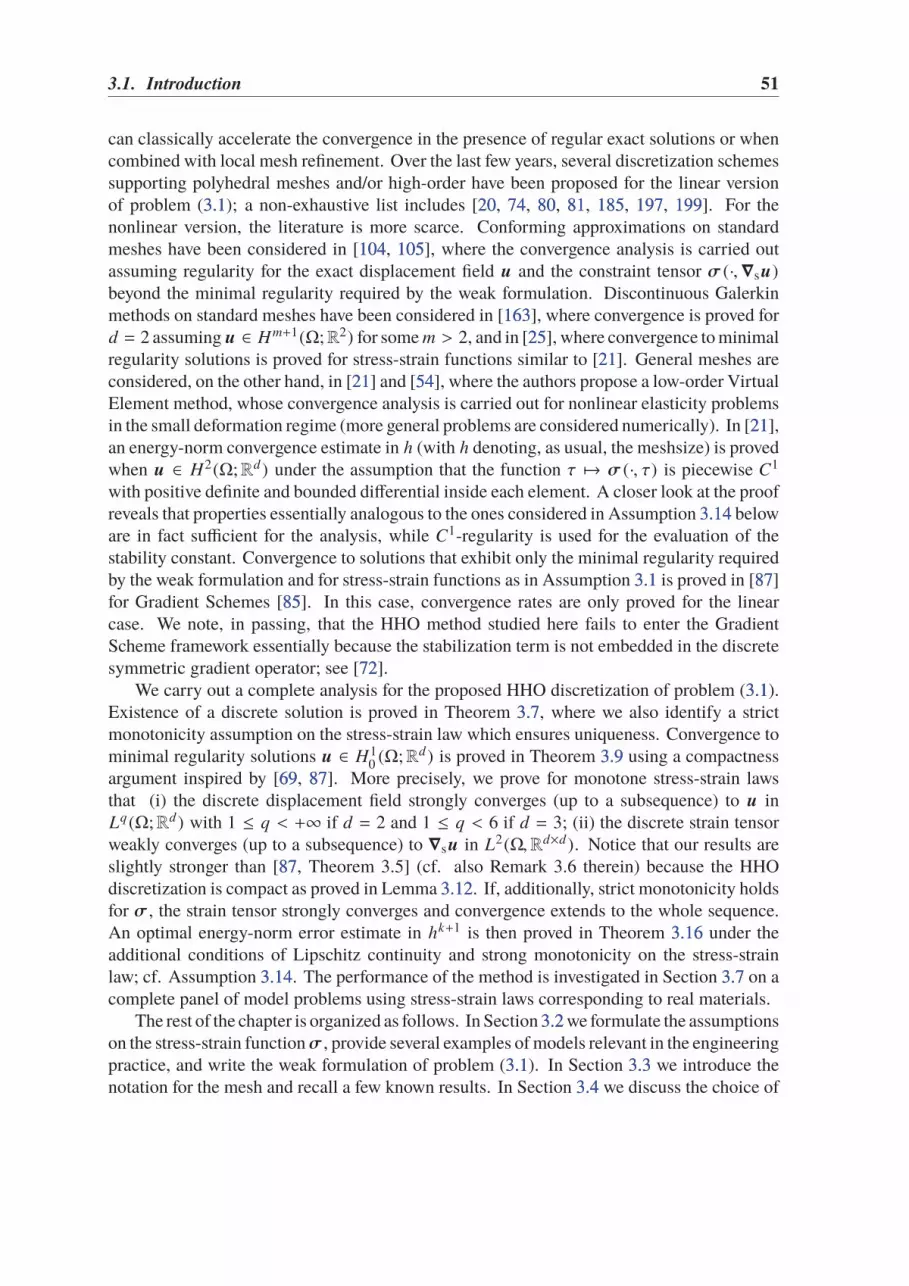
3.1. Introduction 51
can classically accelerate the convergence in the presence of regular exact solutions or whencombined with local mesh refinement. Over the last few years, several discretization schemessupporting polyhedral meshes and/or high-order have been proposed for the linear versionof problem (3.13.1); a non-exhaustive list includes [2020, 7474, 8080, 8181, 185185, 197197, 199199]. For thenonlinear version, the literature is more scarce. Conforming approximations on standardmeshes have been considered in [104104, 105105], where the convergence analysis is carried outassuming regularity for the exact displacement field u and the constraint tensor σ (·,∇su)
beyond the minimal regularity required by the weak formulation. Discontinuous Galerkinmethods on standard meshes have been considered in [163163], where convergence is proved ford = 2 assuming u ∈ Hm+1(Ω;R2) for some m > 2, and in [2525], where convergence to minimalregularity solutions is proved for stress-strain functions similar to [2121]. General meshes areconsidered, on the other hand, in [2121] and [5454], where the authors propose a low-order VirtualElement method, whose convergence analysis is carried out for nonlinear elasticity problemsin the small deformation regime (more general problems are considered numerically). In [2121],an energy-norm convergence estimate in h (with h denoting, as usual, the meshsize) is provedwhen u ∈ H2(Ω;Rd) under the assumption that the function τ 7→ σ (·, τ) is piecewise C1
with positive definite and bounded differential inside each element. A closer look at the proofreveals that properties essentially analogous to the ones considered in Assumption 3.143.14 beloware in fact sufficient for the analysis, while C1-regularity is used for the evaluation of thestability constant. Convergence to solutions that exhibit only the minimal regularity requiredby the weak formulation and for stress-strain functions as in Assumption 3.13.1 is proved in [8787]for Gradient Schemes [8585]. In this case, convergence rates are only proved for the linearcase. We note, in passing, that the HHO method studied here fails to enter the GradientScheme framework essentially because the stabilization term is not embedded in the discretesymmetric gradient operator; see [7272].
We carry out a complete analysis for the proposed HHO discretization of problem (3.13.1).Existence of a discrete solution is proved in Theorem 3.73.7, where we also identify a strictmonotonicity assumption on the stress-strain law which ensures uniqueness. Convergence tominimal regularity solutions u ∈ H1
0 (Ω;Rd) is proved in Theorem 3.93.9 using a compactnessargument inspired by [6969, 8787]. More precisely, we prove for monotone stress-strain lawsthat (i) the discrete displacement field strongly converges (up to a subsequence) to u inLq(Ω;Rd) with 1 ≤ q < +∞ if d = 2 and 1 ≤ q < 6 if d = 3; (ii) the discrete strain tensorweakly converges (up to a subsequence) to ∇su in L2(Ω,Rd×d). Notice that our results areslightly stronger than [8787, Theorem 3.5] (cf. also Remark 3.6 therein) because the HHOdiscretization is compact as proved in Lemma 3.123.12. If, additionally, strict monotonicity holdsfor σ , the strain tensor strongly converges and convergence extends to the whole sequence.An optimal energy-norm error estimate in hk+1 is then proved in Theorem 3.163.16 under theadditional conditions of Lipschitz continuity and strong monotonicity on the stress-strainlaw; cf. Assumption 3.143.14. The performance of the method is investigated in Section 3.73.7 on acomplete panel of model problems using stress-strain laws corresponding to real materials.
The rest of the chapter is organized as follows. In Section 3.23.2 we formulate the assumptionson the stress-strain functionσ , provide several examples of models relevant in the engineeringpractice, and write the weak formulation of problem (3.13.1). In Section 3.33.3 we introduce thenotation for the mesh and recall a few known results. In Section 3.43.4 we discuss the choice of

52 Chapter 3. Nonlinear elasticity
DOFs, formulate the local reconstructions and the discrete problem. The main results, statedand proved in Section 3.53.5, are collected in Theorems 3.73.7, 3.93.9, and 3.163.16 below. In Section 3.63.6we show that the HHO method satisfies on each mesh element a discrete counterpart of theprinciple of virtual work, and that interface tractions obey the law of action and reaction.Section 3.73.7 contains numerical tests. Finally, Appendix 3.83.8 contains the proofs of intermediatetechnical results.
3.2 Setting and examples
For the stress-strain function, we make the followingAssumption 3.1 (Stress-strain function I). The stress-strain function σ : Ω × Rd×d
sym → Rd×dsym
is a Caratheodory function, namely
σ (x, ·) is continuous on Rd×dsym for a.e. x ∈ Ω, (3.2a)
σ (·, τ) is measurable on Ω for all τ ∈ Rd×dsym, (3.2b)
and it holds σ (·, 0) ∈ L2(Ω;Rd×d). Moreover, there exist real numbers σ, σ ∈ (0,+∞) suchthat, for a.e. x ∈ Ω, and all τ, η ∈ Rd×d
sym , the following conditions hold:
‖σ (x, τ) − σ (x, 0)‖d×d ≤ σ ‖τ‖d×d, (growth) (3.2c)
σ (x, τ) : τ ≥ σ ‖τ‖2d×d, (coercivity) (3.2d)
(
σ (x, τ) − σ (x, η))
:(
τ − η) ≥ 0, (monotonicity) (3.2e)
where τ : η ≔∑d
i, j=1 τi, jηi, j and ‖τ‖2d×d≔ τ : τ.
We next discuss a number of meaningful models that satisfy the above assumptions.Example 3.2 (Linear elasticity). The linear elasticity model corresponds to
σ (·,∇su ) = C (·)∇su,
where C is a fourth order tensor. Being linear, the previous stress-strain relation clearlysatisfies Assumption 3.13.1 provided that C is uniformly elliptic. A particular case of theprevious stress-strain relation is the usual linear elasticity Cauchy stress tensor
σ (∇su ) = λ tr(∇su )I d + 2µ∇su, (3.3)
where tr(τ) ≔ τ : I d and λ ≥ 0, µ > 0 are the Lamé’s parameters.Example 3.3 (Hencky–Mises model). The nonlinear Hencky–Mises model of [105105, 157157]corresponds to the stress-strain relation
σ (∇su ) = λ(dev(∇su )) tr(∇su )I d + 2µ(dev(∇su ))∇su, (3.4)
where λ and µ are the nonlinear Lamé’s scalar functions and dev : Rd×dsym → R defined by
dev(τ) = tr(τ2) − 1d
tr(τ)2 is the deviatoric operator. Conditions on λ and µ such that σsatisfies Assumption 3.13.1 can be found in [1313, 2121].
3.2. Setting and examples 53
Example 3.4 (An isotropic damage model). The isotropic damage model of [5050] correspondsto the stress-strain relation
σ (·,∇su ) = (1 − D(∇su ))C (·)∇su, (3.5)
where D : Rd×dsym → R is the scalar damage function and C is a fourth-order symmetric and
uniformly elliptic tensor. If there exists a continuous and bounded function f : [0,+∞) →[a, b] for some 0 < a ≤ b, such that s ∈ [0,+∞) → s f (s) is non-decreasing and, for allτ ∈ Rd×d
sym , D(τ) = 1− f ( |τ |), the damage model constitutive relation satisfies Assumption 3.13.1.In the numerical experiments of Section 3.73.7 we will also consider the following model,
relevant in engineering applications, which however does not satisfy Assumption 3.13.1 ingeneral.Example 3.5 (The second-order elasticity model). The nonlinear second-order isotropicelasticity model of [6666, 124124, 135135] corresponds to the stress-strain relation
σ (∇su ) = λ tr(∇su )I d + 2µ∇su
+ B tr((∇su )2)I d + 2B tr(∇su )∇su + C tr(∇su )2I d + A(∇su )2, (3.6)
where λ and µ are the standard Lamé’s parameter, and A, B,C ∈ R are the second-ordermoduli.
Remark 3.6 (Energy density functions). Examples 3.23.2, 3.33.3, and 3.53.5, used in numerical tests ofSection 3.73.7, can be interpreted in the framework of hyperelasticity. Hyperelasticity is a typeof constitutive model for ideally elastic materials in which the stress-strain relation derivesfrom a stored energy density function Ψ : Rd×d
sym → R, namely
σ (τ) ≔∂Ψ(τ)
∂τ.
The stored energy density function leading to the linear Cauchy stress tensor (3.33.3) is
Ψlin(τ) ≔λ
2tr(τ)2
+ µ tr(τ2), (3.7)
while, in the Hencky–Mises model (3.43.4), it is defined such that
Ψhm(τ) ≔α
2tr(τ)2
+ Φ(dev(τ)). (3.8)
Here α ∈ (0,+∞), while Φ : [0,+∞) → R is a function of class C2 satisfying, for somepositive constants C1, C2, and C3,
C1 ≤ Φ′(ρ) < α, |ρΦ′′(ρ) | ≤ C2, and Φ′(ρ) + 2ρΦ′′(ρ) ≥ C3 ∀ρ ∈ [0,+∞). (3.9)
Deriving the energy density function (3.83.8) yields the stress-strain relation (3.43.4) with nonlinearLamé’s functions µ(ρ) ≔ Φ′(ρ) and λ(ρ) ≔ α − Φ′(ρ). Taking α = λ + µ and Φ(ρ) = µρin (3.83.8) leads to the linear case. Finally, the second-order elasticity model (3.63.6) is obtainedby adding third-order terms to the linear stored energy density function defined in (3.73.7):
Ψsnd(τ) ≔λ
2tr(τ)2
+ µ tr(
τ2)
+
C
3tr(τ)3
+ B tr(τ) tr(τ2) +A
3tr(τ3). (3.10)

54 Chapter 3. Nonlinear elasticity
The weak formulation of problem (3.13.1) that will serve as a starting point for the develop-ment and analysis of the HHO method reads
Find u ∈ H10 (Ω;Rd) such that, for all v ∈ H1
0 (Ω;Rd), a(u, v ) =
∫
Ω
f · v, (3.11)
where H10 (Ω;Rd) is the zero-trace subspace of H1(Ω;Rd) and the function a : H1
0 (Ω;Rd) ×H1
0 (Ω;Rd) → R is such that
a(v, w ) ≔
∫
Ω
σ (x,∇sv (x)) : ∇sw (x)dx.
Throughout the rest of the chapter, to alleviate the notation, we omit the dependence on thespace variable x and the differential dx from integrals.
3.3 Notation and basic results
We consider refined sequences of general polytopal meshes as in [8585, Definition 7.2] matchingthe regularity requirements detailed in [8282, Definition 3]. The main points are summarizedhereafter. Denote byH ⊂ R+∗ a countable set of meshsizes having 0 as its unique accumulationpoint, and let (Th)h∈H be a refined mesh sequence where each Th is a finite collection ofnonempty disjoint open polyhedral elements T with boundary ∂T such thatΩ =
⋃
T∈Th T andh = maxT∈Th hT with hT diameter of T .
For each h ∈ H , let Fh be a set of faces with disjoint interiors which partitions themesh skeleton, i.e.,
⋃
F∈Fh F =⋃
T∈Th ∂T . A face F is defined here as a hyperplanar
closed connected subset of Ω with positive (d−1)-dimensional Hausdorff measure such that(i) either there exist distinct T1,T2 ∈ Th such that F ⊂ ∂T1 ∩ ∂T2 and F is called an interfaceor (ii) there exists T ∈ Th such that F ⊂ ∂T ∩ Γ and F is called a boundary face. Interfacesare collected in the set F i
hand boundary faces in F b
h, so that Fh ≔ F i
h∪ F b
h. For all T ∈ Th,
FT ≔ F ∈ Fh : F ⊂ ∂T denotes the set of faces contained in ∂T and, for all F ∈ FT , nTF
is the unit normal to F pointing out of T .Mesh regularity holds in the sense that, for all h ∈ H , Th admits a matching simplicial
submesh Th and there exists a real number > 0 such that, for all h ∈ H , (i) for any simplexS ∈ Th of diameter hS and inradius rS, hS ≤ rS and (ii) for any T ∈ Th and all S ∈ Th suchthat S ⊂ T , hT ≤ hS.
Let X be a mesh element or face. For an integer l ≥ 0, we denote by Pld(X ;R) the space
spanned by the restriction to X of scalar-valued, d-variate polynomials of total degree l. TheL2-projector πl
X: L1(X ;R) → Pl
d(X ;R) is defined such that, for all v ∈ L1(X ;R),
∫
X
(πlXv − v)w = 0 ∀w ∈ Pl
d (X ;R). (3.12)
When dealing with the vector-valued polynomial space Pld(X ;Rd) or with the tensor-valued
polynomial space Pld(X ;Rd×d), we use the boldface notation π l
Xfor the corresponding L2-
orthogonal projectors acting component-wise.

3.4. The Hybrid High-Order method 55
On regular mesh sequences, we have the following optimal approximation propertiesfor πl
T(for a proof, cf. [7676, Lemmas 1.58 and 1.59] and, in a more general framework, [7070,
Lemmas 3.4 and 3.6]): There exists a real number Capp > 0 such that, for all s ∈ 0, . . . , l+1,all h ∈ H , all T ∈ Th, and all v ∈ H s (T ;R),
|v − πlTv |Hm (T ;R) ≤ Capphs−m
T |v |H s (T ;R) ∀m ∈ 0, . . . , s, (3.13a)
and, if s ≥ 1,
|v − πlTv |Hm (FT ;R) ≤ Capph
s−m− 12
T|v |H s (T ;R) ∀m ∈ 0, . . . , s − 1, (3.13b)
with Hm(FT ;R) denoting the broken hilbert space on the faces of T . Other useful geometricand functional analytic results on regular mesh sequences can be found in [7676, Chapter 1]and [6969, 7070].
At the global level, we define broken versions of polynomial and Sobolev spaces. Inparticular, for an integer l ≥ 0, we denote by Pl
d(Th;R), Pl
d(Th;Rd), and Pl
d(Th;Rd×d),
respectively, the space of scalar-valued, vector-valued, and tensor-valued broken polynomialfunctions on Th of total degree l. The space of broken vector-valued polynomial functions oftotal degree l on the trace of the mesh on the domain boundary Γ is denoted by Pl
d(F b
h;Rd).
Similarly, for an integer s ≥ 1, H s (Th;R), H s (Th;Rd), and H s (Th;Rd×d) are the scalar-valued, vector-valued, and tensor-valued broken Sobolev spaces of index s.
Throughout the rest of the chapter, for X ⊂ Ω, we denote by ‖·‖X the standard normin L2(X ;R), with the convention that the subscript is omitted whenever X = Ω. The samenotation is used for the vector- and tensor-valued spaces L2(X ;Rd) and L2(X ;Rd×d).
3.4 The Hybrid High-Order method
In this section we define the space of DOFs and the local reconstructions, and we state thediscrete problem.
3.4.1 Degrees of freedom
Let a polynomial degree k ≥ 1 be fixed. The DOFs for the displacement are collected in thespace
U kh≔ *,×T∈Th P
kd (T ;Rd)+- × *,×F∈Fh P
kd (F;Rd)+- ,
see Figure 3.13.1. Observe that naming U kh
the space of DOFs involves a shortcut: the actualDOFs can be chosen in several equivalent ways (polynomial moments, point values, etc.),and the specific choice does not affect the following discussion. Details concerning the actualchoice made in the implementation are given in Section 3.73.7 below.
For a generic collection of DOFs in U kh, we use the classical HHO underlined notation
vh≔
(
(vT )T∈Th, (vF )F∈Fh)
. We also denote by vh ∈ Pkd(Th;Rd) and vΓ,h ∈ Pk
d(F b
h;Rd) (not
underlined) the broken polynomial functions such that
(vh) |T = vT ∀T ∈ Th and (vΓ,h) |F = vF ∀F ∈ F bh .

56 Chapter 3. Nonlinear elasticity
••••
•• ••
••••
••••
••••
••••
••
•• ••
••••••
•• •• ••
••••••
••••••
••••••
••••••
••
••••
••
••••
••
Figure 3.1: Local DOFs for k = 1 (left) and k = 2 (right). Shaded DOFs can be locally eliminated by staticcondensation when solving linearized versions of problem (3.213.21).
The restrictions ofU kh
and vh
to a mesh elementT are denoted byU kT
and vT=
(
vT, (vF )F∈FT)
,respectively. The space U k
his equipped with the following discrete strain semi-norm:
‖vh‖ǫ,h ≔ *.,
∑
T∈Th‖v
h‖2ǫ,T+/-
1/2
, ‖vh‖2ǫ,T ≔ ‖∇svT ‖2
T +
∑
F∈FTh−1
F ‖vF − vT ‖2F . (3.14)
The DOFs corresponding to a given function v ∈ H1(Ω;Rd) are obtained by means ofthe reduction map I k
h: H1(Ω;Rd) → U k
hsuch that
I khv ≔
(
(πkT v )T∈Th, (π
kFv )F∈Fh
)
, (3.15)
where we remind the reader that πkT
and πkF
denote the L2-orthogonal projectors on Pkd(T ;Rd)
and Pkd(F;Rd), respectively. For all mesh elements T ∈ Th, the local reduction map I k
T:
H1(T ;Rd) → U kT
is obtained by a restriction of I kh, and is therefore such that for all v ∈
H1(T ;Rd)
I kT v =
(
πkT v, (π
kFv )F∈FT
)
. (3.16)
3.4.2 Local reconstructions
We introduce symmetric gradient and displacement reconstruction operators devised at theelement level that are instrumental to the formulation of the method.
Let a mesh element T ∈ Th be fixed. The local symmetric gradient reconstruction operator
Gks,T : U k
T→ Pk
d (T ;Rd×dsym )
is obtained by solving the following pure traction problem:c3: For a given local collectionof DOFs v
T=
(
vT, (vF )F∈FT) ∈ U k
T, find Gk
s,T vT∈ Pk
d(T ;Rd×d
sym ) such that, for all τ ∈P
kd(T ;Rd×d
sym ),∫
T
Gks,T vT
: τ = −∫
T
vT · (∇·τ) +∑
F∈FT
∫
F
vF · (τnTF ) (3.17a)
=
∫
T
∇svT : τ +∑
F∈FT
∫
F
(vF − vT ) · (τnTF ). (3.17b)

3.4. The Hybrid High-Order method 57
The right-hand side of (3.17a3.17a) is designed to resemble an integration by parts formula wherethe role of the function represented by the DOFs in v
Tis played by vT inside the volumetric
integral and by (vF )F∈FT inside boundary integrals. The reformulation (3.17b3.17b), obtainedintegrating by parts the first term in the right-hand side of (3.17a3.17a), highlights the fact that ourmethod is nonconforming, as the second addend accounts for the difference between vF andvT .
The definition of the symmetric gradient reconstruction is justified observing that, usingthe definitions (3.163.16) of the local reduction map I k
Tand (3.123.12) of the L2-orthogonal projectors
πkT
and πkF
in (3.17a3.17a), one can prove the following commuting property: For all T ∈ Th andall v ∈ H1(T ;Rd),
Gks,T I k
T v = πkT (∇sv ). (3.18)
As a result of (3.183.18) and (3.133.13), Gks,T I k
Thas optimal approximation properties in Pk
d(T ;Rd×d
sym ).
From Gks,T , one can define the local displacement reconstruction operator
r k+1T : U k
T→ Pk+1
d (T ;Rd)
such that, for all vT∈ U k
T,∇sr
k+1T
vT
is the orthogonal projection ofGks,T vT
on∇sPk+1d
(T ;Rd) ⊂P
kd(T ;Rd×d
sym ) and rigid-body motions are prescribed according to [7474, Eq. (15)]. More pre-
cisely, we let r k+1T
vT
be such that for all w ∈ Pk+1d
(T ;Rd) it holds
∫
T
(∇srk+1T v
T− Gk
s,T vT) : ∇sw = 0
and, denoting by ∇ss the skew-symmetric part of the gradient operator, we have
∫
T
r k+1T v
T=
∫
T
vT,
∫
T
∇ssrk+1T v
T=
∑
F∈FT
∫
F
1
2(vF ⊗ nTF − nT F ⊗ vF ) .
Notice that, for a given vT∈ U k
T, the displacement reconstruction r k+1
Tv
Tis a vector-valued
polynomial function one degree higher than the element-based DOFs vT . It was provedin [7474, Lemma 2] that r k+1
TI k
Thas optimal approximation properties in Pk+1
d(T ;Rd).
In what follows, we will also need the global counterparts of the discrete gradient anddisplacement operators Gk
s,h : U kh→ Pk
d(Th;Rd×d
sym ) and r k+1h
: U kh→ Pk+1
d(Th;Rd) defined
setting, for all vh∈ U k
hand all T ∈ Th,
(Gks,hvh
)|T = Gks,T vT
, (r k+1h v
h) |T = r k+1
T vT. (3.19)
3.4.3 Discrete problem
We define the following subspace of U kh
strongly accounting for the homogeneous Dirichletboundary condition (3.1b3.1b):
U kh,D ≔
v
h∈ U k
h: vF = 0 ∀F ∈ F b
h
, (3.20)
58 Chapter 3. Nonlinear elasticity
and we notice that the map ‖·‖ǫ,h defined by (3.143.14) is a norm onU kh,D. The HHO approximation
of problem (3.113.11) reads:
Find uh ∈ U kh,D such that, for all v
h∈ U k
h,D,
ah(uh, vh) ≔ Ah(uh, vh
) + sh(uh, vh) =
∫
Ω
f · vh, (3.21)
where the consistency contribution Ah : U kh× U k
h→ R and the stability contribution sh :
U kh× U k
h→ R are respectively defined setting
Ah(uh, vh) ≔
∫
Ω
σ (·, Gks,huh) : Gk
s,hvh,
sh(uh, vh) ≔
∑
T∈ThsT (uT, vT
), sT (uT, vT) ≔
∑
F∈FT
γ
hF
∫
F
∆kT FuT · ∆
kTFvT
. (3.22)
The scaling parameter γ > 0 in (3.223.22) can depend on σ and σ but is independent of themeshsize h. In the numerical tests of Section 3.73.7 we take γ = 2µ for the linear (3.33.3) andsecond-order (3.63.6) models and γ = 2µ(0) for the Hencky–Mises model (3.43.4). In sT , wepenalize in a least-square sense the face-based residual ∆k
T F : U kT→ Pk
d(F;Rd) such that, for
all T ∈ Th, all vT∈ U k
T, and all F ∈ FT ,
∆kTFvT
≔ πkF (r k+1
T vT− vF ) − πk
T (r k+1T v
T− vT ). (3.23)
This particular choice ensures that ∆kTF vanishes whenever its argument is of the form I k
Tw
with w ∈ Pk+1d
(T ;Rd), a crucial property to obtain an energy-norm error estimate in hk+1; cf.Theorem 3.163.16 below. Additionally, sh is stabilizing in the sense that the following uniformnorm equivalence holds (the proof is a straightforward modification of [7474, Lemma 4]; cf.also Corollary 6 therein): There exists a real number η > 0 independent of h such that, forall v
h∈ U k
h,D,
η−1‖vh‖2ǫ,h ≤ ‖Gk
s,hvh‖2+ sh(v
h, v
h) ≤ η‖v
h‖2ǫ,h. (3.24)
By (3.2d3.2d), this implies the coercivity of ah.
3.5 Analysis
In this section we carry out a complete analysis of the method. To alleviate the notation,inside the proofs we abridge into a . b the inequality a ≤ Cb with real number C > 0independent of h.
3.5.1 Existence and uniqueness
We start by discussing existence and uniqueness of the discrete solution.

3.5. Analysis 59
Theorem 3.7 (Existence and uniqueness of a discrete solution). Let Assumption 3.13.1 hold
and let (Th)h∈H be a regular mesh sequence. Then, for all h ∈ H , there exists at least one
solution uh ∈ U kh,D to problem (3.213.21). Additionally, if the stress-strain function σ is strictly
monotone (i.e., if the inequality in (3.2e3.2e) is strict for τ , η), the solution is unique.
Proof. 1) Existence. We follow the argument of [6464, Theorem 3.3]. If (E, (·, ·)E, ‖·‖E )
is a Euclidean space and Φ : E → E is a continuous map such that (Φ(x),x)E‖x‖E → +∞, as
‖x‖E → +∞, then Φ is surjective. We take E = U kh,D, endowed with the inner product
(vh, w
h)ǫ,h ≔
∑
T∈Th
*.,∫
T
∇svT : ∇swT +
∑
F∈FT
1
hF
∫
F
(vF − vT ) · (wF − wT )+/- ,
and we define Φ : U kh,D → U k
h,D such that, for all vh∈ U k
h,D, (Φ(vh), w
h)ǫ,h = ah(v
h, w
h)
for all wh∈ U k
h,D. The coercivity (3.2d3.2d) of σ together with the norm equivalence (3.243.24)
yields (Φ(vh), v
h)ǫ,h ≥ min1, σ η−1‖v
h‖2ǫ,h
for all vh∈ U k
h,D, so that Φ is surjective. Let
now yh∈ U k
h,D be such that (yh, w
h)ǫ,h =
∫
Ωf · wh for all w
h∈ U k
h,D. By the surjectivity of
Φ, there exists uh ∈ U kh,D such that Φ(uh) = y
h. By definition of Φ and y
h, uh is a solution
to the problem (3.213.21).2) Uniqueness. Let uh,1, uh,2 ∈ U k
h,D solve (3.213.21). We assume uh,1 , uh,2 and proceed bycontradiction. Subtracting (3.213.21) for uh,2 from (3.213.21) for uh,1, it is inferred that ah(uh,1, vh
)−a(uh,2, vh
) = 0 for all vh∈ U k
h,D. Hence in particular, taking vh= uh,1 − uh,2 we obtain that
ah(uh,1, uh,1 − uh,2) − ah(uh,2, uh,1 − uh,2) = 0.
On the other hand, owing to the strict monotonicity of σ and to the fact that the bilinear formsh is positive semidefinite, we have that
ah(uh,1, uh,1 − uh,2) − ah(uh,2, uh,1 − uh,2)
=
∫
Ω
(
σ (·, Gks,huh,1) − σ (·, Gk
s,huh,2))
: Gks,h(uh,1 − uh,2)
+ sh(uh,1 − uh,2, uh,1 − uh,2) > 0.
Hence, uh,1 = uh,2 and the conclusion follows.
Remark 3.8 (Strict monotonicity of the stress-strain function). The strict monotonicity as-sumption is fulfilled, e.g., by the Hencky–Mises model (3.43.4) and by the damage model (3.53.5)when D(τ) = 1 − f (|τ |), with f continuous, bounded, and such that [0,+∞) ∋ s 7→ s f (s)
is strictly increasing. We observe, in passing, that the strict monotonicity is weaker than thestrong monotonicity (3.40b3.40b) used in Theorem 3.163.16 below to prove error estimates.

60 Chapter 3. Nonlinear elasticity
3.5.2 Convergence
We now consider the convergence to solutions that only exhibit the minimal regularity requiredby the variational formulation (3.113.11). More specifically, in this section we prove the followingTheorem 3.9 (Convergence). Let Assumption 3.13.1 hold, let k ≥ 1, and let (Th)h∈H be a
regular mesh sequence. Further assume the existence of a real number CK > 0 independent
of h but possibly depending on Ω, , and on k such that, for all vh∈ U k
h,D,
‖vh‖ + ‖∇hvh‖ ≤ CK‖vh‖ǫ,h, (3.25)
where ∇h denotes the broken gradient on H1(Th;Rd). For all h ∈ H , let uh ∈ U kh,D be a
solution to the discrete problem (3.213.21) on Th. Then, for all q such that 1 ≤ q < +∞ if d = 2or 1 ≤ q < 6 if d = 3, as h → 0 it holds, up to a subsequence,
• uh → u strongly in Lq(Ω;Rd),
• Gks,huh → ∇su weakly in L2(Ω;Rd×d),
where u ∈ H10 (Ω;Rd) solves the weak formulation (3.113.11). Moreover, if we assume strict
monotonicity for σ (i.e., the inequality in (3.2e3.2e) is strict for τ , η), it holds that
• Gks,huh → ∇su strongly in L2(Ω;Rd×d).
Finally, if the solution to (3.113.11) is unique, convergence extends to the whole sequence.
Some remarks are of order before proceeding with the proof of Theorem 3.93.9.
Remark 3.10 (Existence of a solution to the continuous problem). A side result of theexistence of discrete solutions proved in Theorem 3.73.7 together with the convergence resultsof Theorem 3.93.9 is the existence of a solution to the weak formulation (3.113.11).
Remark 3.11 (Discrete Korn inequality). In Proposition 3.203.20 below we give a proof of thediscrete Korn inequality (3.253.25) based on the results of [3939], which require further assumptionson the mesh. While we have the feeling that these assumptions could probably be relaxed,we postpone this topic to a future work. Notice that inequality (3.253.25) is not required to provethe error estimate of Theorem 3.163.16 below.
The proof of Theorem 3.93.9 hinges on two technical results stated hereafter: a discreteRellich–Kondrachov Lemma (cf. [4040, Theorem 9.16]) and a proposition showing the approx-imation properties of the discrete symmetric gradient Gk
s,h defined by (3.193.19). Their proofsare given in Appendix 3.83.8.Lemma 3.12 (Discrete compactness). Let the assumptions of Theorem 3.93.9 hold. Let
(vh)h∈H ∈ (U k
h,D)h∈H , and assume that there is a real number C ≥ 0 such that
‖vh‖ǫ,h ≤ C ∀h ∈ H . (3.26)
Then, for all q such that 1 ≤ q < +∞ if d = 2 or 1 ≤ q < 6 if d = 3, the sequence
(vh)h∈H ∈ (Pkd(Th;Rd))h∈H is relatively compact in Lq(Ω;Rd). As a consequence, there is
a function v ∈ Lq(Ω;Rd) such that as h → 0, up to a subsequence, vh → v strongly in
Lq(Ω;Rd).
3.5. Analysis 61
Proof. See Appendix 3.8.23.8.2.
Proposition 3.13 (Consistency of the discrete symmetric gradient operator). Let (Th)h∈Hbe a regular mesh sequence, and let Gk
s,h be as in (3.193.19) with Gks,T defined by (3.173.17) for all
T ∈ Th.
1) Strong consistency. For all v ∈ H1(Ω;Rd) with I kh
defined by (3.153.15), it holds as h → 0
Gks,hI k
hv → ∇sv strongly in L2(Ω;Rd×d). (3.27)
2) Sequential consistency. For all h ∈ H and all τ ∈ H1(Ω;Rd×dsym ), denoting by γn (τ) the
normal trace of τ on Γ, it holds
limh→0
*, maxvh∈Uk
h, ‖vh ‖ǫ,h=1
∫
Ω
Gks,hvh
: τ + vh · (∇·τ) −∫
Γ
vΓ,h · γn (τ)+- = 0, (3.28)
Proof. See Appendix 3.8.33.8.3.
We are now ready to prove convergence.
Proof of Theorem 3.93.9. The proof is subdivided into four steps: in Step 1 we prove a uniforma priori bound on the solutions of the discrete problem (3.213.21); in Step 2 we infer the existenceof a limit for the sequence of discrete solutions and investigate its regularity; in Step 3 weshow that this limit solves the continuous problem (3.113.11); finally, in Step 4 we prove strongconvergence.
Step 1: A priori bound. We start by showing the following uniform a priori bound onthe sequence of discrete solutions:
‖uh‖ǫ,h ≤ C‖ f ‖, (3.29)
where the real number C > 0 only depends on Ω, σ, γ, , and k. Making vh= uh in (3.213.21)
and using the coercivity property (3.2d3.2d) of σ in the left-hand side together with the Cauchy–Schwarz inequality in the right-hand side yields
∑
T∈Th
*.,σ ‖Gks,TuT ‖
2T +
∑
F∈Fh
γ
hF
‖∆kTFuT ‖
2F+/- ≤ ‖ f ‖‖uh‖.
Owing to the norm equivalence (3.243.24), and using the discrete Korn inequality (3.253.25) toestimate the right-hand side of the previous inequality, it is inferred that
η−1 min(1, σ)‖uh‖2ǫ,h ≤ ‖ f ‖‖uh‖ ≤ CK‖ f ‖‖uh‖ǫ,h.
Dividing by ‖uh‖ǫ,h yields (3.293.29) with C = η min(1, σ)−1CK.Step 2: Existence of a limit and regularity. Let 1 ≤ q < +∞ if d = 2 or 1 ≤
q < 6 if d = 3. Owing to the a priori bound (3.293.29) and the norm equivalence (3.243.24), thesequences (‖uh‖ǫ,h)h∈H and (‖Gk
s,huh‖)h∈H are uniformly bounded. Therefore, Lemma 3.123.12
62 Chapter 3. Nonlinear elasticity
and the Kakutani theorem [4040, Theorem 3.17] yield the existence of u ∈ Lq(Ω;Rd) andG ∈ L2(Ω;Rd×d) such that as h → 0, up to a subsequence,
uh → u strongly in Lq(Ω;Rd) and Gks,huh → G weakly in L2(Ω;Rd×d).
This together with the fact that uh,Γ = 0 on Γ, shows that, for any τ ∈ H1(Ω;Rd×dsym ),
∫
Ω
G : τ + u · (∇·τ)
= limh→0
∫
Ω
Gks,huh : τ + uh · (∇·τ) −
∫
Γ
uh,Γ · γn (τ)
≤ limh→0
*,‖uh‖ǫ,h maxvh∈Uk
h, ‖vh ‖ǫ,h=1
∫
Ω
Gks,hvh
: τ + vh · (∇·τ) −∫
Γ
vh,Γ · γn (τ)+-
= 0.
(3.30)
To infer the previous limit we have used the uniform bound (3.293.29) on ‖uh‖ǫ,h and the sequentialconsistency (3.283.28) of Gk
s,h. Applying (3.303.30) with τ ∈ C∞c (Ω;Rd×d
sym ) leads to∫
Ω
G : τ + u · (∇·τ) = 0,
thus G = ∇su in the sense of distributions on Ω. As a result, owing to the isomorphismof Hilbert spaces between H1(Ω;Rd) and v ∈ L2(Ω;Rd) | ∇sv ∈ L2(Ω;Rd×d
sym ) proved
in [8989, Theorem 3.1], we have u ∈ H1(Ω;Rd). Using again (3.303.30) with τ ∈ H1(Ω;Rd×dsym )
and integrating by parts, we obtain∫
Γ
γ(u ) · γn (τ) = 0
with γ(u ) denoting the trace of u . As the set γn (τ) : τ ∈ H1(Ω;Rd×dsym ) is dense in
L2(Γ;Rd), we deduce that γ(u ) = 0 on Γ. In conclusion, with convergences up to asubsequence,
u ∈ H10 (Ω;Rd), uh → u strongly in Lq(Ω;Rd)
Gks,huh → ∇su weakly in L2(Ω;Rd×d).
Step 3: Identification of the limit. Let us now prove that u is a solution to (3.113.11).The growth property (3.2c3.2c) on σ and the bound on (‖Gk
s,huh‖)h∈H ensure that the sequence
(σ (·, Gks,huh))h∈H is bounded in L2(Ω;Rd×d
sym ). Hence, there exists η ∈ L2(Ω;Rd×dsym ) such
that, up to a subsequence as h → 0,
σ (·, Gks,huh) → η weakly in L2(Ω;Rd×d). (3.31)
Plugging into (3.213.21) vh= I k
hφ, with φ ∈ C∞
c (Ω;Rd), gives∫
Ω
σ (·, Gks,huh) : Gk
s,hI khφ =
∫
Ω
f · πkhφ − sh(uh, I k
hφ), (3.32)

3.5. Analysis 63
with πkh
denoting the L2-projector on the broken polynomial spaces Pkd(Th;Rd) and sh defined
by (3.223.22). Using the Cauchy–Schwarz inequality followed by the norm equivalence (3.243.24) tobound the first factor, we infer
|sh(uh, I khφ) | ≤ sh(uh, uh)
1/2sh(I khφ, I k
hφ)1/2 ≤ ‖uh‖ǫ,hsh(I k
hφ, I khφ)
1/2. (3.33)
It was proved in [7474, Eq. (35)] using the optimal approximation properties of r k+1T
I kT
that itholds for all h ∈ H , all T ∈ Th, all v ∈ H k+2(T ;Rd), and all F ∈ FT that
h−1/2F
‖∆kTF I k
T v ‖F . hk+1T ‖v ‖Hk+2(T ;Rd ), (3.34)
with ∆kTF defined by (3.233.23). As a consequence, recalling the definition (3.223.22) of sh, we have
the following convergence result:
∀v ∈ H1(Ω;Rd) ∩ H2(Th;Rd), limh→0
sh(I khv, I k
hv ) = 0. (3.35)
Recalling the a priori bound (3.293.29) on the discrete solution and the convergence prop-erty (3.353.35), it follows from (3.333.33) that |sh(uh, I k
hφ) | → 0 as h → 0. Additionally, by the
approximation property (3.13a3.13a) of the L2-projector, one has πkhφ → φ strongly in L2(Ω;Rd)
and, by virtue of Proposition 3.133.13, that Gks,hI k
hφ → ∇sφ strongly in L2(Ω;Rd×d). Thus, we
can pass to the limit h → 0 in (3.323.32) and obtain∫
Ω
η : ∇sφ =
∫
Ω
f · φ. (3.36)
By density of C∞c (Ω;Rd) in H1
0 (Ω;Rd), this relation still holds if φ ∈ H10 (Ω;Rd). On the
other hand, plugging vh= uh into (3.213.21) and using the fact that sh(uh, uh) ≥ 0, we obtain
Th ≔
∫
Ω
σ (·, Gks,huh) : Gk
s,huh ≤∫
Ω
f · uh.
Thus, using the previous bound, the strong convergence uh → u , and (3.363.36), it is inferredthat
limh→0Th ≤
∫
Ω
f · u =∫
Ω
η : ∇su . (3.37)
We now use the monotonicity assumption on σ and the Minty trick [152152] to prove thatη = σ (·,∇su ). Let Λ ∈ L2(Ω;Rd×d) and write, using the monotonicity (3.2e3.2e) of σ , theconvergence (3.313.31) of σ (·, Gk
s,huh), and the bound (3.373.37),
0 ≤ limh→0
(∫
Ω
(σ (·, Gks,huh) − σ (·,Λ)) : (Gk
s,huh − Λ)
)
≤∫
Ω
(η − σ (·,Λ)) : (∇su − Λ).
(3.38)Applying the previous relation with Λ = ∇su ± t∇sv , for t > 0 and v ∈ H1
0 (Ω;Rd), anddividing by t, leads to
0 ≤ ±∫
Ω
(η − σ (·,∇su ∓ t∇sv )) : ∇sv .
64 Chapter 3. Nonlinear elasticity
Owing to the growth property (3.2c3.2c) and the Caratheodory property (3.2a3.2a) of σ , we can lett → 0 and pass the limit inside the integral and then inside the argument of σ . In conclusion,for all v ∈ H1
0 (Ω;Rd), we infer
∫
Ω
σ (·,∇su ) : ∇sv =
∫
Ω
η : ∇sv =
∫
Ω
f · v,
where we have used (3.363.36) with φ = v in order to obtain the second equality. The aboveequation shows that η = σ (·,∇su ) and that u solves (3.113.11).
Step 4: Strong convergence. We prove that if σ is strictly monotone then Gks,huh → ∇su
strongly in L2(Ω;Rd×d). We define the function Dh : Ω→ R such that
Dh ≔ (σ (·, Gks,huh) − σ (·,∇su )) : (Gk
s,huh − ∇su ).
For all h ∈ H , the functionDh is non-negative as a result of the monotonicity property (3.2e3.2e)and, by (3.383.38) with Λ = ∇su , it is inferred that limh→0
∫
ΩDh = 0. Hence, (Dh)h∈H
converges to 0 in L1(Ω) and, therefore, also almost everywhere on Ω up to a subsequence.Let us take x ∈ Ω such that the above mentioned convergence hold at x. Developing theproducts in Dh and using the coercivity and growth properties (3.2d3.2d) and (3.2c3.2c) of σ , onehas
Dh(x) ≥ σ ‖Gks,huh(x)‖2
d×d − 2σ ‖Gks,huh(x)‖d×d ‖∇su (x)‖d×d + σ ‖∇su (x)‖2
d×d .
Since the right hand side is quadratic in ‖Gks,huh(x)‖d×d and (Dh(x))h∈H is bounded, we
deduce that also (Gks,huh(x))h∈H is bounded. Passing to the limit in the definition of Dh(x)
yields(
σ (x, Lx) − σ (x,∇su (x)))
:(
Lx − ∇su (x))
= 0,
where Lx is an adherence value of (Gks,huh(x))h∈H . The strict monotonicity assumption
forces Lx = ∇su (x) to be the unique adherence value of (Gks,huh(x))h∈H , and therefore the
sequence converges to this value. As a result,
Gks,huh → ∇su a.e. on Ω. (3.39)
Using (3.373.37) together with Fatou’s Lemma, we see that
limh→0
∫
Ω
σ (·, Gks,huh) : Gk
s,huh =
∫
Ω
σ (·,∇su ) : ∇su .
Moreover, owing to (3.393.39), (σ (·, Gks,huh) : Gk
s,huh)h∈H is a non-negative sequence convergingalmost everywhere on Ω. Using [8484, Lemma 8.4] we see that this sequence also converges inL1(Ω) and, therefore, it is equi-integrable in L1(Ω). Thus, the coercivity (3.2d3.2d) of σ ensuresthat (Gk
s,huh)h∈H is equi-integrable in L2(Ω;Rd×d) and Vitali’s theorem shows that
Gks,huh → ∇su strongly in L2(Ω;Rd×d).
This concludes the proof.

3.5. Analysis 65
3.5.3 Error estimate
We next estimate the order of convergence of the method for solutions that display furtherregularity beyond that required by the variational formulation. We stipulate the followingadditional assumptions on the stress-strain function σ .Assumption 3.14 (Stress-strain relation II). There exist real numbers σ∗, σ∗ ∈ (0,+∞) suchthat, for a.e. x ∈ Ω, and all τ, η ∈ Rd×d
sym ,
‖σ (x, τ) − σ (x, η)‖d×d ≤ σ∗‖τ − η‖d×d, (Lipschitz continuity) (3.40a)(
σ (x, τ) − σ (x, η))
:(
τ − η) ≥ σ∗‖τ − η‖2d×d . (strong monotonicity) (3.40b)
Remark 3.15 (Lipschitz continuity and strong monotonocity). It has been proved in [1313,Lemma 4.1] that, under the assumptions (3.93.9), the stress-strain tensor function for the Hencky–Mises model is strongly monotone and Lipschitz-continuous, namely Assumption 3.143.14 holds.Also the isotropic damage model satisfies Assumption 3.143.14 if the damage function in (3.53.5)is, for instance, such that D(|τ |) = 1 − (1 + |τ |)− 1
2 .
Theorem 3.16 (Error estimate). Let Assumptions 3.13.1 and 3.143.14 hold, and let (Th)h∈H be a
regular mesh sequence. Let u be the unique solution to (3.13.1). Let a polynomial degree k ≥ 1be fixed, and, for all h ∈ H , let uh be the unique solution to (3.213.21) on the mesh Th. Then,
under the additional regularity u ∈ H k+2(Th;Rd) and σ (·,∇su ) ∈ H k+1(Th;Rd×d), it holds
‖∇su−Gks,huh‖+sh(uh, uh)
12 ≤ Chk+1
(
‖u ‖Hk+2(Th ;Rd ) + ‖σ (·,∇su )‖Hk+1(Th ;Rd×d )
)
, (3.41)
where C is a positive constant depending only on Ω, k, the mesh regularity parameter , the
real numbers σ , σ , σ∗, σ∗ appearing in (3.23.2) and in (3.403.40), and an upper bound of ‖ f ‖.Remark 3.17 (Locking-free error estimate). The proposed scheme, although different fromthe one of [7474], is robust in the quasi-incompressible limit. The reason is that, as a result ofthe commuting property (3.183.18), we have πk
T(∇·v ) = tr(Gk
s,T I kTv ). Thus, considering, e.g., the
linear elasticity stress-strain relation (3.33.3), we can proceed as in [7474, Theorem 8] in order toprove that, when u ∈ H k+2(Th;Rd) and ∇·u ∈ H k+1(Th;R), and choosing γ = 2µ, it holds
(2µ)1/2‖∇su − Gk
s,huh‖ ≤ Chk+1(
2µ‖u ‖Hk+2(Th ;Rd ) + λ‖∇·u ‖Hk+1(Th ;R)
)
,
with real number C > 0 independent of h, µ and λ. The previous bound leads to a locking-free estimate; see [7474, Remark 9]. Note that the locking-free nature of polyhedral elementmethods has also been observed in [197197] for the Weak Galerkin method and in [2020] for theVirtual Element method.
Proof of Theorem 3.163.16. For the sake of conciseness, throughout the proof we let uh ≔ I khu
and use the following abridged notations for the constraint field and its approximations:
ς ≔ σ (·,∇su ) and, for all T ∈ Th, ςT ≔ σ (·, Gks,TuT ) and ςT ≔ σ (·, Gk
s,T uT ).
First we want to show that (3.413.41) holds assuming that
‖uh − uh‖ǫ,h . hk+1(
‖u ‖Hk+2(Th ;Rd ) + ‖ς ‖Hk+1(Th ;Rd×d )
)
. (3.42)
66 Chapter 3. Nonlinear elasticity
Using the triangle inequality, we obtain
‖Gks,huh − ∇su ‖ + sh(uh, uh)
1/2 ≤ ‖Gks,h(uh − uh)‖ + sh(uh − uh, uh − uh)
1/2
+ ‖Gks,h uh − ∇su ‖ + sh(uh, uh)
1/2.(3.43)
Using the norm equivalence (3.243.24) followed by (3.423.42) we obtain for the terms in the first lineof (3.433.43)
‖Gks,h(uh − uh)‖ + sh(uh − uh, uh − uh)
1/2. hk+1
(
‖u ‖Hk+2(Th ;Rd ) + ‖ς ‖Hk+1(Th ;Rd×d )
)
.
For the terms in the second line, using the approximation properties of Gks,h resulting
from (3.183.18) together with (3.13a3.13a) for the first addend and (3.343.34) for the second, we get
‖Gks,h uh − ∇su ‖ + sh(uh, uh)
1/2. hk+1‖u ‖Hk+2(Th ;Rd ) .
It only remains to prove (3.423.42), which we do in two steps: in Step 1 we prove a basic estimatein terms of a conformity error, which is then bounded in Step 2.
Step 1: Basic error estimate. Using for all T ∈ Th the strong monotonicity (3.40b3.40b) withτ = Gk
s,T uT and η = Gks,TuT , we infer
‖Gks,h(uh − uh)‖2
.
∑
T∈Th
∫
T
(ςT − ςT ) : Gks,T (uT − uT ).
Owing to the norm equivalence (3.243.24) and the previous bound, we get
‖ uh − uh‖2ǫ,h .
∑
T∈Th
∫
T
(ςT − ςT ) : Gks,T (uT − uT ) + sh(uh − uh, uh − uh)
= ah(uh, uh − uh) −∫
Ω
f · (uh − uh).
where we have used the discrete problem (3.213.21) to conclude. Hence, dividing by ‖ uh − uh‖ǫ,hand passing to the supremum in the right-hand side, we arrive at the following error estimate:
‖ uh − uh‖ǫ,h . supvh∈Uk
h,D, ‖vh ‖ǫ,h=1
Eh(vh), (3.44)
with conformity error such that, for all vh∈ U k
h,D,
Eh(vh) ≔
∑
T∈Th
∫
T
ςT : Gks,T vT
−∫
Ω
f · vh + sh(uh, vh). (3.45)
Step 2: Bound of the conformity error. We bound the quantity Eh(vh) defined above
for a generic vh∈ U k
h,D. Denote by T1, T2, and T3 the three addends in the right-hand sideof (3.453.45).

3.5. Analysis 67
Using for all T ∈ Th the definition (3.173.17) of Gks,T with τ = πk
TςT , we have that
T1 =
∑
T∈Th
*.,∫
T
ςT : ∇svT +
∑
F∈FT
∫
F
πkT ςTnTF · (vF − vT )
+/- , (3.46)
where we have used the fact that ∇svT ∈ Pk−1d
(T ;Rd×d) together with the definition (3.123.12) ofthe orthogonal projector to cancel πk
Tin the first term.
On the other hand, using the fact that f = −∇·ς a.e. inΩ and integrating by parts elementby element, we get that
T2 = −∑
T∈Th
*.,∫
T
ς : ∇svT +
∑
F∈FT
∫
F
ςnTF · (vF − vT )+/- , (3.47)
where we have additionally used that ς |T1nT1F +ς |T2nT2F = 0 for all interfaces F ⊂ ∂T1∩∂T2
and that vF vanishes on Γ (cf. (3.203.20)) to insert vF into the second term.Summing (3.463.46) and (3.473.47), taking absolute values, and using the Cauchy–Schwarz
inequality to bound the right-hand side, we infer that
|T1 + T2 | ≤ *.,∑
T∈Th
(
‖ς − ςT ‖2T + hT ‖ς − πk
T ςT ‖2∂T
)+/-1/2
‖vh‖ǫ,h. (3.48)
It only remains to bound the first factor. Let a mesh element T ∈ Th be fixed. Using theLipschitz continuity (3.40a3.40a) with τ = Gk
s,T uT and η = ∇su and the optimal approximation
properties of Gks,T I k
Tresulting from (3.183.18) together with (3.13a3.13a) with m = 1 and s = k + 2,
leads to
‖ς − ςT ‖T . ‖∇su − Gks,T uT ‖T . hk+1‖u ‖Hk+2(T ;Rd ), (3.49)
which provides an estimate for the first term inside the summation in the right-hand sideof (3.483.48). To estimate the second term, we use the triangle inequality, the discrete traceinequality of [7676, Lemma 1.46], and the boundedness of πk
Tto write
h1/2T‖ς − πk
T ςT ‖∂T . ‖πkT (ς − ςT )‖T + h
1/2T‖ς − πk
Tς ‖∂T ≤ ‖ς − ςT ‖T + h1/2T‖ς − πk
Tς ‖∂T .
The first term in the right-hand side is bounded by (3.493.49). For the second, using the approxima-tion properties (3.13b3.13b) of πk
Twith m = 0 and s = k+1, we get h
1/2T‖ς − πk
Tς ‖∂T . hk+1‖ς ‖Hk+1(T ;Rd×d )
so that, in conclusion,
h1/2T‖ς − πk
T ςT ‖∂T . hk+1(
‖u ‖Hk+2(T ;Rd ) + ‖ς ‖Hk+1(T ;Rd×d )
)
. (3.50)
Plugging the estimates (3.493.49) and (3.503.50) into (3.483.48) finally yields
|T1 + T2 | . hk+1(
‖u ‖Hk+2(Th ;Rd ) + ‖ς ‖Hk+1(Th ;Rd×d )
)
‖vh‖ǫ,h. (3.51)

68 Chapter 3. Nonlinear elasticity
It only remains to bound T3 = sh(uh, vh). Using the Cauchy–Schwarz inequality, the defini-
tion (3.223.22) of sh, the approximation property (3.343.34) of ∆kTF , and the norm equivalence (3.243.24),
we infer
|T3 | . *.,∑
T∈Th
∑
F∈FT
γ
hF
‖∆kTF uT ‖
2F+/-
1/2
sh(vh, v
h)
1/2. hk+1‖u ‖Hk+2(Th ;Rd ) ‖vh
‖ǫ,h. (3.52)
Using (3.513.51) and (3.523.52), we finally get that, for all vh∈ U k
h,D,
Eh(vh) . hk+1
(
‖u ‖Hk+2(Th ;Rd ) + ‖ς ‖Hk+1(Th ;Rd×d )
)
‖vh‖ǫ,h. (3.53)
Thus, using (3.533.53) to bound the right-hand side of (3.443.44), (3.423.42) follows.
3.6 Local principle of virtual work and law of action and
reaction
We show in this section that the solution of the discrete problem (3.213.21) satisfies inside eachelement a local principle of virtual work with numerical tractions that obey the law of actionand reaction. This property is important from both the mathematical and engineering pointsof view, and it can simplify the derivation of a posteriori error estimators based on equilibratedtractions; see, e.g., [33, 158158]. It is worth emphasizing that local equilibrium properties on theprimal mesh are a distinguishing feature of hybrid (face-based) methods: the derivation ofsimilar properties for vertex-based methods usually requires to perform reconstructions on adual mesh.
Define, for all T ∈ Th, the space
Dk∂T ≔ ×
F∈FTP
kd (F;Rd),
as well as the boundary difference operator δk∂T
: U kT→ Dk
∂Tsuch that, for all v
T∈ U k
T,
δk∂Tv
T= (δk
FvT)F∈FT ≔ (vF − vT )F∈FT .
The following proposition shows that the stabilization can be reformulated in terms of bound-ary differences.Proposition 3.18 (Reformulation of the local stabilization bilinear form). For all mesh
elements T ∈ Th, the local stabilization bilinear form sT defined by (3.223.22) satisfies, for all
uT, vT∈ U k
T,
sT (uT, vT) = sT ((0, δk
∂TuT ), (0, δk
∂Tv
T)). (3.54)
Proof. Let a mesh element T ∈ Th be fixed. Using the fact that r k+1T
I kTvT = vT for all
vT ∈ Pkd(T )d (this because r k+1
TI k
Tis a projector on Pk+1
d(T ;Rd), cf. [7474, Eq. (20)]) together
3.6. Local principle of virtual work and law of action and reaction 69
with the linearity of r k+1T
, it is inferred that, for all F ∈ FT , the face-based residual definedby (3.233.23) satisfies
∆kTFvT
= πkF (r k+1
T (0, δk∂Tv
T) − δk
FvT) − πk
T rk+1T (0, δk
∂Tv
T) = ∆k
TF (0, δk∂Tv
T)
for all vT∈ U k
T. Plugging this expression into (3.223.22) yields the assertion.
Define now the boundary residual operator Rk∂T
: U kT→ Dk
∂Tsuch that, for all v
T∈ U k
T,
Rk∂Tv
T≔ (Rk
TFv
T)F∈FT satisfies
−∑
F∈FT
∫
F
RkTFvT
· αF = sT ((0, δk∂Tv
T), (0, α∂T )) ∀α∂T ∈ Dk
∂T . (3.55)
Problem (3.553.55) is well-posed, and computing RkTF
vT
requires to invert the boundary massmatrix.Lemma 3.19 (Local principle of virtual work and law of action and reaction). Denote by
uh ∈ U kh,D a solution of problem (3.213.21) and, for all T ∈ Th and all F ∈ FT , define the
numerical traction
TTF (uT ) ≔ −πkTσ (·, Gk
s,TuT )nTF + RkTFuT .
Then, for all T ∈ Th we have the following discrete principle of virtual work: For all
vT ∈ Pkd(T ;Rd),
∫
T
σ (·, Gks,TuT ) : ∇svT +
∑
F∈FT
∫
F
TTF (uT ) · vT =
∫
T
f · vT, (3.56)
and, for any interface F ∈ FT1 ∩ FT2 , the numerical tractions satisfy the law of action and
reaction:
TT1F (uT1) +TT2F (uT2
) = 0. (3.57)
Proof. For all T ∈ Th, use the definition (3.173.17) of Gks,T vT
with τ = πkTσ (·Gk
s,TuT ) in Ah and
the rewriting (3.543.54) of sT together with the definition (3.553.55) of RkTF
to infer that it holds, forall v
h∈ U k
h,
∫
Ω
f · vh = Ah(uh, vh) + sh(uh, vh
)
=
∑
T∈Th
∫
T
σ (·, Gks,TuT ) : ∇svT
+
∑
T∈Th
∑
F∈FT
∫
F
(πkTσ (·, Gk
s,TuT )nTF − RkTFuT ) · (vF − vT ),
where to cancel πkT
inside the first integral in the second line we have used the fact that∇svT ∈ Pk−1
d(T ;Rd×d) for all T ∈ Th. Selecting v
hsuch that vT spans Pk
d(T ;Rd) for a selected
mesh element T ∈ Th while vT ′ ≡ 0 for all T ′ ∈ Th \ T and vF ≡ 0 for all F ∈ Fh,we obtain (3.563.56). On the other hand, selecting v
hsuch that vT ≡ 0 for all T ∈ Th, vF
spans Pkd(F;Rd) for a selected interface F ∈ FT1 ∩ FT2 , and vF ′ ≡ 0 for all F′ ∈ Fh \ F
yields (3.573.57).
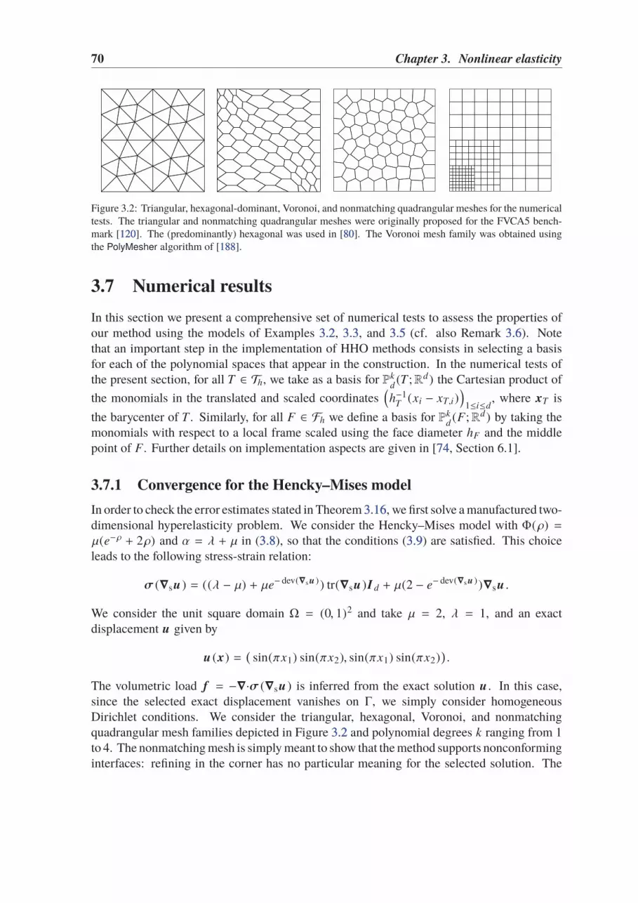
70 Chapter 3. Nonlinear elasticity
Figure 3.2: Triangular, hexagonal-dominant, Voronoi, and nonmatching quadrangular meshes for the numericaltests. The triangular and nonmatching quadrangular meshes were originally proposed for the FVCA5 bench-mark [120120]. The (predominantly) hexagonal was used in [8080]. The Voronoi mesh family was obtained usingthe PolyMesher algorithm of [188188].
3.7 Numerical results
In this section we present a comprehensive set of numerical tests to assess the properties ofour method using the models of Examples 3.23.2, 3.33.3, and 3.53.5 (cf. also Remark 3.63.6). Notethat an important step in the implementation of HHO methods consists in selecting a basisfor each of the polynomial spaces that appear in the construction. In the numerical tests ofthe present section, for all T ∈ Th, we take as a basis for Pk
d(T ;Rd) the Cartesian product of
the monomials in the translated and scaled coordinates(
h−1T
(xi − xT,i))
1≤i≤d, where xT is
the barycenter of T . Similarly, for all F ∈ Fh we define a basis for Pkd(F;Rd) by taking the
monomials with respect to a local frame scaled using the face diameter hF and the middlepoint of F. Further details on implementation aspects are given in [7474, Section 6.1].
3.7.1 Convergence for the Hencky–Mises model
In order to check the error estimates stated in Theorem 3.163.16, we first solve a manufactured two-dimensional hyperelasticity problem. We consider the Hencky–Mises model with Φ(ρ) =
µ(e−ρ + 2ρ) and α = λ + µ in (3.83.8), so that the conditions (3.93.9) are satisfied. This choiceleads to the following stress-strain relation:
σ (∇su ) = ((λ − µ) + µe− dev(∇su )) tr(∇su )I d + µ(2 − e− dev(∇su ))∇su .
We consider the unit square domain Ω = (0, 1)2 and take µ = 2, λ = 1, and an exactdisplacement u given by
u (x) =(
sin(πx1) sin(πx2), sin(πx1) sin(πx2))
.
The volumetric load f = −∇·σ (∇su ) is inferred from the exact solution u . In this case,since the selected exact displacement vanishes on Γ, we simply consider homogeneousDirichlet conditions. We consider the triangular, hexagonal, Voronoi, and nonmatchingquadrangular mesh families depicted in Figure 3.23.2 and polynomial degrees k ranging from 1to 4. The nonmatching mesh is simply meant to show that the method supports nonconforminginterfaces: refining in the corner has no particular meaning for the selected solution. The

3.7. Numerical results 71
x1
x2
u “ 0
σn “ T
p0, 0q
p1, 1q
‚
‚
σn
“0
σn
“0
(a) Description
1.5 −0.2
(b) σ1,1
1 −1
(c) σ1,2
5 3
(d) σ2,2
Figure 3.3: Tensile test description and resulting stress components for the linear case. Values in 105Pa
x1
x2
u “ 0
σn “ T
p0, 0q
p1, 1q
‚
‚
σn
“0
σn
“0
(a) Description
1 −1
(b) σ1,1
0.8 0
(c) σ1,2
3 −3
(d) σ2,2
Figure 3.4: Shear test description and resulting stress components for the linear case. Values in 105Pa
initialization of our iterative linearization procedure (Newton scheme) is obtained solving thelinear elasticity model. This initial guess leads to a 40% reduction of the number of iterationswith respect to a null initial guess. The energy-norm orders of convergence (OCV) displayedin the third column of Tables 3.13.1–3.43.4 at the end of the chapter are in agreement with thetheoretical predictions. In particular, it is observed that the optimal convergence in hk+1 isreached for the triangular, nonmatching Cartesian, and hexagonal meshes for 1 ≤ k ≤ 3,whereas for k = 4 the asymptotic convergence order does not appear to have been reachedin the last mesh refinement. It can also be observed in Table 3.23.2 that the convergence rateexceeds the estimated one on the locally refined Cartesian mesh for k = 1 and k = 2. For thesake of completeness, we also display in the fourth column of Tables 3.13.1–3.43.4 the L2-normof the error defined as the difference between the L2-projection πk
hu of the exact solution
on Pkd(Th;Rd) and the broken polynomial function uh obtained from element-based DOFs,
while in the fifth column we display the corresponding observed convergence rates. In thiscase, orders of convergence up to hk+2 are observed.
3.7.2 Tensile and shear test cases
We next consider the two test cases schematically depicted in Figures 3.33.3 and 3.43.4. Onthe unit square domain Ω, we solve problem (3.1a3.1a) considering three different models ofhyperelasticity (see Remark 3.63.6):

72 Chapter 3. Nonlinear elasticity
(i) Linear. The linear model corresponding to the stored energy density function (3.73.7) withLamé’s parameters
λ = 11 × 105Pa, µ = 82 × 104Pa. (3.58)
(ii) Hencky–Mises. The Hencky–Mises model (3.43.4) obtained by takingΦ(ρ) = µ(ρ2 + (1 + ρ)
1/2)
and α = λ + µ in (3.83.8), with λ, µ as in (3.583.58) (also in this case the conditions (3.93.9)hold). This choice leads to
σ (∇su ) = ((λ +µ
2) − µ
2(1 + dev(∇su ))−
1/2)) tr(∇su )I d
+ µ(1 + (1 + dev(∇su ))−1/2)∇su .
(3.59)
The Lamé’s functions of the previous relation are inspired from those proposed in [2121,Section 5.1]. In particular, the function µ(ρ) = µ(1 + (1 + dev(∇su ))−1/2) correspondsto the Carreau law for viscoplastic materials.
(iii) Second-order. The second-order model (3.63.6) with Lamé’s parameter as in (3.583.58) andsecond-order moduli
A = 11 × 106Pa, B = −48 × 105Pa, C = 13.2 × 10⁵Pa.
These values correspond to the estimates provided in [124124] for the Armco Iron. Werecall that the second-order elasticity stress-strain relation does not satisfy in generalthe assumptions under which we are able to prove the convergence and error estimates.In particular, we observe that the stored energy density function defined in (3.103.10) is notconvex.
The bottom part of the boundary of the domain is assumed to be fixed, the normal stress isequal to zero on the two lateral parts, and a traction is imposed at the top of the boundary.So, mixed boundary conditions are imposed as follows
u = 0 on x ∈ Γ, x2 = 0,σn = T on x ∈ Γ, x2 = 1,σn = 0 on x ∈ Γ, x1 = 0,σn = 0 on x ∈ Γ, x1 = 1.
For the tensile case, we impose a vertical traction at the top of the boundary equal toT = (0, 3.2 × 10⁵Pa). This type of boundary conditions produces large normal stresses (i.e.,the diagonal components of σ) and minor shear stresses (i.e., the off-diagonal components ofσ). It can be observed in Figure 3.33.3, where the components of the stress tensor are depictedfor the linear case. In Figure 3.53.5 we plot the stress norm on the deformed domain obtainedfor the three hyperelasticity models. The results of Fig. 3.33.3, 3.43.4, 3.53.5, and 3.63.6 are obtained ona mesh with 3584 triangles (corresponding to a typical mesh-size of 3.84 × 10⁻³) and withpolynomial degree k = 2. Obviously, the symmetry of the results is visible, and we observethat the three displacement fields are very close. This is motivated by the fact that, with ourchoice of the parameters in (3.583.58) and in (3.593.59), the linear model exactly corresponds to thelinear approximation at the origin of the nonlinear ones. The maximum value of the stress

3.7. Numerical results 73
(a) Linear (b) Hencky–Mises (c) Second order
Figure 3.5: Tensile test case: Stress norm on the deformed domain. Values in 105Pa
(a) Linear (b) Hencky–Mises (c) Second order
Figure 3.6: Shear test case: Stress norm on the deformed domain. Values in 104Pa
concentrates on the two bottom corners due to the homogeneous Dirichlet condition thattotally locks the displacement when x1 = 0. The repartition of the stress on the domain withthe second-order model is visibly different from those obtained with the linear and Hencky–Mises models. At the energy level, we also have a higher difference between the second-ordermodel and the linear one since |Elin − Ehm |/Elin = 0.44% while |Elin − Esnd |/Elin = 4.45%,where E• is the total elastic energy obtained by integrating over the domain the strain energydensity functions defined by (3.73.7), (3.83.8), and (3.103.10):
E• ≔
∫
Ω
Ψ•, with • ∈ lin, hm, snd.
The reference values for the total energy, used in Figure 3.73.7 in order to assess convergence,are obtained on a fine Cartesian mesh having a mesh-size of 1.95 × 10⁻³ and k = 3. For theshear case, we consider an horizontal traction equal toT = (4.5×10⁴Pa, 0) which induces thestress pattern illustrated in Figure 3.43.4. The computed stress norm on the deformed domain isdepicted in Figure 3.63.6, and we can see that the displacement fields associated with the threemodels are very close as for the tensile test case. Here, the maximum values of the stress arelocalized in the lower part of the domain near the lateral parts. Unlike the tensile test, the

74 Chapter 3. Nonlinear elasticity
difference between the three models is tiny as confirmed by the elastic energy equal to 3180 J,3184 J, and 3190 J respectively. The decreasing of the energy difference in comparison withthe previous test can be explained by the fact that the value of the Neumann boundary dataon the top is divided by a factor 7 in order to obtain maximum displacements roughly equalto 15%.
3.8 Appendix: Technical results
This appendix contains the proof of technical results.
3.8.1 Discrete Korn inequality
Proposition 3.20 (Discrete Korn inequality). Assume that the mesh further verifies the as-
sumption of [3939, Theorem 4.2] if d = 2 and [3939, Theorem 5.2] if d = 3. Then, the discrete
Korn inequality (3.253.25) holds.
Proof. Using the broken Korn inequality [3939, Eq. (1.22)] on H1(Th;Rd) followed by theCauchy–Schwarz inequality, one has
‖vh‖2+ ‖∇hvh‖2
. ‖∇s,hvh‖2+
∑
F∈F ih
h−1F ‖[vh]F ‖2
F
+ supm∈P1
d(Th ;Rd ), ‖γn (m)‖Γ=1
(∫
Γ
γ(vh) · γn (m)
)2
. ‖∇s,hvh‖2+
∑
F∈F ih
h−1F ‖[vh]F ‖2
F +
∑
F∈F bh
‖vh |F ‖2F .
(3.60)
For an interface F ∈ FT1∩FT2 , we have introduced the jump [vh]F ≔ vT1−vT2 . Thus, using thetriangle inequality, we get ‖[vh]F ‖F ≤ ‖vF−vT1 ‖F+‖vF−vT2 ‖F . For a boundary face F ∈ F b
h
such that F ∈ FT ∩ F bh
for some T ∈ Th we have, on the other hand, ‖vh |F ‖F = ‖vF − vT ‖F
since vF ≡ 0 (cf. (3.203.20)). Using these relations in the right-hand side of (3.603.60) and rearrangingthe sums leads to
‖vh‖2+ ‖∇hvh‖2
.
∑
T∈Th
*.,‖∇svT ‖2T +
∑
F∈FT∩F ih
h−1F ‖vF − vT ‖2
F+/- + h
∑
F∈F bh
h−1F ‖vF − vh |F ‖2
F
. max1, dΩ∑
T∈Th
*.,‖∇svT ‖2T +
∑
F∈FTh−1
F ‖vF − vT ‖2F+/- ,
where dΩ denotes the diameter of Ω. Owing to the definition (3.143.14) of the discrete strainseminorm, the latter yields the assertion.

3.8. Appendix: Technical results 75
0.000 0.005 0.010 0.015 0.020 0.025 0.030
21,532
21,538
21,544
21,550k = 1 Triangulark = 1 Voronoi
k = 2 Triangulark = 2 Voronoi
k = 3 Triangulark = 3 VoronoiElin = 21532 J
(a) Linear, tensile test
0.000 0.005 0.010 0.015 0.020 0.025 0.030
3,180
3,184
3,188
3,192k = 1 Triangulark = 1 Voronoi
k = 2 Triangulark = 2 Voronoi
k = 3 Triangulark = 3 VoronoiElin = 3180 J
(b) Linear, shear test
0.000 0.005 0.010 0.015 0.020 0.025 0.030
21,627
21,633
21,639
21,645k = 1 Triangulark = 1 Voronoi
k = 2 Triangulark = 2 Voronoi
k = 3 Triangulark = 3 VoronoiEhm = 21627 J
(c) Hencky–Mises, tensile test
0.000 0.005 0.010 0.015 0.020 0.025 0.030
3,184
3,188
3,192
3,196k = 1 Triangulark = 1 Voronoi
k = 2 Triangulark = 2 Voronoi
k = 3 Triangulark = 3 VoronoiEhm = 3184 J
(d) Hencky–Mises, shear test
0.000 0.005 0.010 0.015 0.020 0.025 0.030
22,490
22,500
22,510
22,520k = 1 Triangulark = 1 Voronoi
k = 2 Triangulark = 2 Voronoi
k = 3 Triangulark = 3 VoronoiEsnd = 22490 J
(e) Second-order, tensile test
0.000 0.005 0.010 0.015 0.020 0.025 0.030
3,190
3,194
3,198
3,202k = 1 Triangulark = 1 Voronoi
k = 2 Triangulark = 2 Voronoi
k = 3 Triangulark = 3 VoronoiEsnd = 3190 J
(f) Second-order, shear test
Figure 3.7: Energy vs h, tensile and shear test cases

76 Chapter 3. Nonlinear elasticity
3.8.2 Discrete compactness
Proof of Lemma 3.123.12. In the proof we use the same notation for functions in L2(Ω;Rd) ⊂L1(Ω;Rd) and for their extension by zero outside Ω. Let (v
h)h∈H ∈ (U k
h,D)h∈H besuch that (3.263.26) holds. Define the space of integrable functions with bounded variationBV(Rd) ≔ v ∈ L1(Rd;Rd) | ‖v ‖BV < +∞, where
‖v ‖BV ≔
d∑
i=1
sup
∫
Rd
v · ∂iφ | φ ∈ C∞c (Rd;Rd), ‖φ‖L∞(Rd ;Rd ) ≤ 1
.
Here, ∂iφ denotes the i-th column of ∇φ. Let φ ∈ C∞c (Rd;Rd) with ‖φ‖L∞(Rd ;Rd ) ≤ 1.
Integrating by parts and using the fact that∑
T∈Th∑
F∈FT∫
F(vF · φ)nT F = 0, we have that
∫
Rd
vh · ∂iφ =∑
T∈Th
∫
T
((∇φ)TvT )i
= −∑
T∈Th
*.,∫
T
((∇vT )Tφ)i +
∑
F∈FT
∫
F
(vF · φ − vT · φ)(nTF )i+/-
≤∑
T∈Th
*.,∫
T
d∑
j=1
|(∇vT ) ji | +∑
F∈FT
∫
F
d∑
j=1
|(vF − vT ) j (nTF )i |+/- ,where, in order to pass to the third line, we have used ‖φ‖L∞(Rd ;Rd ) ≤ 1. Therefore, summingover i ∈ 1, ..., d, observing that, for all T ∈ Th and all F ∈ FT , we have
∑di=1 |(nTF )i | ≤ d
1/2,and using the Lebesgue embeddings arising from the Hölder inequality on bounded domain,leads to
‖vh‖BV .
∑
T∈Th
*.,|T |1/2d‖∇vT ‖T +
∑
F∈FT|F |1/2
d−1‖vF − vT ‖F+/- ,
where |·|d denotes the d-dimensional Hausdorff measure. Moreover, using the Cauchy–Schwarz inequality together with the geometric bound |F |d−1hF . |T |d , we obtain that
‖vh‖BV . |Ω|1/2d
*.,∑
T∈Th
‖∇vT ‖2T +
∑
F∈FTh−1
F ‖vF − vT ‖2F
+/-
1/2
.
Thus, using the discrete Korn inequality (3.253.25), it is readily inferred that
‖vh‖BV . ‖vh‖ǫ,h . 1.
Owing to the Helly selection principle [9999, Section 5.2.3], the sequence (vh)h∈H is relativelycompact in L1(Rd;Rd) and thus in L1(Ω;Rd). It only remains to prove that the sequence isalso relatively compact in Lq(Ω;Rd), with 1 < q < +∞ if d = 2 or 1 < q < 6 if d = 3.

3.8. Appendix: Technical results 77
Owing to the discrete Sobolev embeddings [7171, Proposition 5.4] together with the discreteKorn inequality (3.253.25), it holds, with r = q + 1 if d = 2 and r = 6 if d = 3, that
‖vh‖Lr (Ω;Rd ) .*.,∑
T∈Th
‖∇vT ‖2T +
∑
F∈FTh−1
F ‖vF − vT ‖2F
+/-
1/2
. 1,
Thus, we can complete the proof by means of the interpolation inequality [4040, Remark 2p. 93]. For all h, h′ ∈ H we have with θ ≔ r−q
q(r−1)∈ (0, 1),
‖vh − vh′‖Lq (Ω;Rd ) ≤ ‖vh − vh′‖θL1(Ω;Rd )‖vh − vh′‖1−θ
Lr (Ω;Rd ). ‖vh − vh′‖θL1(Ω;Rd )
.
Therefore, up to a subsequence, (vh)h∈H is a Cauchy sequence in Lq(Ω;Rd), so it converges.
3.8.3 Consistency of the discrete symmetric gradient operator
Proof of Proposition 3.133.13. 1) Strong consistency. We first assume that v ∈ H2(Ω;Rd).Owing to the commuting property (3.183.18) and the approximation property (3.13a3.13a) with m = 1and s = 2, it is inferred that ‖Gk
s,T I kTv − ∇sv ‖T . h‖v ‖H2(T ;Rd ). Squaring, summing over
T ∈ Th, and taking the square root of the resulting inequality gives
‖Gks,hI k
hv − ∇sv ‖ . h‖v ‖H2(Ω;Rd ) . (3.61)
If v ∈ H1(Ω;Rd) we reason by density, namely we take a sequence (v ǫ )ǫ>0 ⊂ H2(Ω;Rd)
that converges to v in H1(Ω;Rd) as ǫ → 0 and, using twice the triangular inequality, wewrite
‖Gks,hI k
hv − ∇sv ‖ ≤ ‖Gks,hI k
h(v − v ǫ )‖ + ‖Gks,hI k
hv ǫ − ∇sv ǫ ‖ + ‖∇s(v − v ǫ )‖.
By (3.613.61), the second term in the right-hand side tends to 0 as h → 0. Moreover, owing tothe commuting property (3.183.18) and the H1-boundedness of πk
T, one has
‖Gks,hI k
h(v − v ǫ )‖ = *.,∑
T∈Th‖πk
T∇s(v − v ǫ )‖2T+/-
1/2
≤ *.,∑
T∈Th‖∇s(v − v ǫ )‖2
T+/-
1/2
≤ ‖∇s(v − v ǫ )‖.
Therefore, taking the supremum limit as h → 0 and then the supremum limit as ǫ → 0,concludes the proof of (3.273.27) (notice that the order in which the limits are taken is important).
2) Sequential consistency. In order to prove (3.283.28) we observe that, by the defini-tions (3.193.19) of Gk
s,h and (3.17b3.17b) of Gks,T one has, for all τ ∈ H1(Ω;Rd×d
sym ) and all vh∈ U k
h,
78 Chapter 3. Nonlinear elasticity
∫
Ω
Gks,hvh
: τ =∑
T∈Th
∫
T
Gks,T vT
: τ
=
∑
T∈Th
∫
T
(Gks,T vT
− ∇svT ) : (τ − π0Tτ) +
∑
T∈Th
∫
T
(Gks,T vT
− ∇svT ) : π0Tτ
+
∑
T∈Th
∫
T
∇svT : τ
= T1 +
∑
T∈Th
∑
F∈FT
∫
F
(vF − vT ) · (π0Tτ)nTF +
∑
T∈Th
∫
T
∇svT : τ
= T1 +
∑
T∈Th
∑
F∈FT
∫
F
(vF − vT ) · (π0Tτ − τ)nTF −
∑
T∈Th
∫
T
vT · (∇·τ)
+
∑
F∈F bh
∫
F
vF · (τnTF )
= T1 + T2 −∫
Ω
vh · (∇·τ) +
∫
Γ
vΓ,h · γn (τ).
(3.62)
To obtain the third equality, we used an element-wise integration by parts together with therelation
∑
T∈Th
∑
F∈FT∩F ih
∫
F
vF · (τnTF ) =∑
F∈F ih
∫
F
vF · (τnT1F + τnT2F ) = 0,
where for all F ∈ F ih, T1,T2 ∈ Th are such that F ⊂ ∂T1∩∂T2. Owing to (3.623.62), the conclusion
follows once we prove that |T1 + T2 | . h‖vh‖ǫ,h‖τ‖H1(Ω;Rd×d ). By (3.13a3.13a) (with m = 0 and
s = 1) we have ‖τ − π0Tτ‖T . hT ‖τ‖H1(T ;Rd×d ) and thus, using the Cauchy–Schwarz and
triangle inequalities followed by the norm equivalence (3.243.24),
|T1 | ≤ *.,∑
T∈Th‖Gk
s,T vT− ∇svT ‖2
T+/-
1/2 *.,∑
T∈Th‖τ − π0
Tτ‖2T+/-
1/2
. h(
‖Gks,hvh
‖2+ ‖v
h‖2ǫ,h
)1/2 ‖τ‖H1(Ω;Rd×d ) . h‖vh‖ǫ,h‖τ‖H1(Ω;Rd×d ) .
(3.63)
In a similar way, we obtain an upper bound for T2. By (3.13b3.13b) (with m = 0 and s = 1), forall F ∈ FT , we have ‖τ − π0
Tτ‖F . h
1/2T‖τ‖H1(T ;Rd×d ) . h
1/2F‖τ‖H1(T ;Rd×d ) and thus, using the
Cauchy–Schwarz inequality,
|T2 | .∑
T∈Th
∑
F∈FTh
1/2F‖vF − vT ‖F ‖τ‖H1(T ;Rd×d ) . h‖v
h‖ǫ,h‖τ‖H1(Ω;Rd×d ) . (3.64)
Owing to (3.633.63) and (3.643.64), the triangle inequality |T1 + T2 | ≤ |T1 | + |T2 | yields theconclusion.

3.8. Appendix: Technical results 79
Table 3.1: Convergence results on the triangular mesh family. OCV stands for order of convergence.
h ‖∇su − Gks,huh ‖ OCV ‖πk
hu − uh ‖ OCV
k = 1
3.07 · 10−2 5.59 · 10−2 — 7.32 · 10−3 —1.54 · 10−2 1.51 · 10−2 1.9 1.05 · 10−3 2.817.68 · 10−3 3.86 · 10−3 1.96 1.34 · 10−4 2.963.84 · 10−3 1.01 · 10−3 1.93 1.7 · 10−5 2.981.92 · 10−3 2.59 · 10−4 1.96 2.15 · 10−6 2.98
k = 2
3.07 · 10−2 1.3 · 10−2 — 1.47 · 10−3 —1.54 · 10−2 1.29 · 10−3 3.35 6.05 · 10−5 4.627.68 · 10−3 2.11 · 10−4 2.6 5.36 · 10−6 3.483.84 · 10−3 2.73 · 10−5 2.95 3.6 · 10−7 3.91.92 · 10−3 3.42 · 10−6 3 2.28 · 10−8 3.98
k = 3
3.07 · 10−2 2.81 · 10−3 — 2.39 · 10−4 —1.54 · 10−2 3.72 · 10−4 2.93 1.95 · 10−5 3.637.68 · 10−3 2.16 · 10−5 4.09 5.47 · 10−7 5.143.84 · 10−3 1.43 · 10−6 3.92 1.66 · 10−8 5.041.92 · 10−3 9.51 · 10−8 3.91 5.34 · 10−10 4.96
k = 4
3.07 · 10−2 1.37 · 10−3 — 1.13 · 10−4 —1.54 · 10−2 5.97 · 10−5 4.54 3.04 · 10−6 5.247.68 · 10−3 1.76 · 10−6 5.07 4.09 · 10−8 6.193.84 · 10−3 6.46 · 10−8 4.77 7.64 · 10−10 5.74

80 Chapter 3. Nonlinear elasticity
Table 3.2: Convergence results on the locally refined mesh family. OCV stands for order of convergence.
h ‖∇su − Gks,huh ‖ OCV ‖πk
hu − uh ‖ OCV
k = 1
0.25 0.13 — 1.9 · 10−2 —0.13 2.64 · 10−2 2.28 2.54 · 10−3 2.9
6.25 · 10−2 4.97 · 10−3 2.41 3.22 · 10−4 2.983.12 · 10−2 9.14 · 10−4 2.44 4.12 · 10−5 2.961.56 · 10−2 1.67 · 10−4 2.45 5.21 · 10−6 2.98
k = 2
0.25 1.88 · 10−2 — 3.79 · 10−3 —0.13 5.05 · 10−3 1.9 3.55 · 10−4 3.42
6.25 · 10−2 6.51 · 10−4 2.96 2.92 · 10−5 3.63.12 · 10−2 6.83 · 10−5 3.25 1.89 · 10−6 3.941.56 · 10−2 6.23 · 10−6 3.45 1.19 · 10−7 3.99
k = 3
0.25 7.84 · 10−3 — 1.41 · 10−3 —0.13 1.09 · 10−3 2.85 7.5 · 10−5 4.23
6.25 · 10−2 8.22 · 10−5 3.73 3.93 · 10−6 4.253.12 · 10−2 5.64 · 10−6 3.86 1.45 · 10−7 4.751.56 · 10−2 3.44 · 10−7 4.04 5.23 · 10−9 4.79
k = 4
0.25 4.35 · 10−3 — 4.68 · 10−4 —0.13 3.65 · 10−4 3.58 3.19 · 10−5 3.87
6.25 · 10−2 1.5 · 10−5 4.6 6.02 · 10−7 5.733.12 · 10−2 5.78 · 10−7 4.69 1.03 · 10−8 5.86
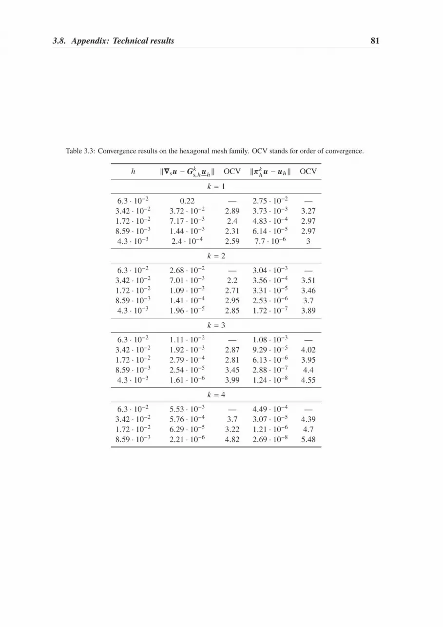
3.8. Appendix: Technical results 81
Table 3.3: Convergence results on the hexagonal mesh family. OCV stands for order of convergence.
h ‖∇su − Gks,huh ‖ OCV ‖πk
hu − uh ‖ OCV
k = 1
6.3 · 10−2 0.22 — 2.75 · 10−2 —3.42 · 10−2 3.72 · 10−2 2.89 3.73 · 10−3 3.271.72 · 10−2 7.17 · 10−3 2.4 4.83 · 10−4 2.978.59 · 10−3 1.44 · 10−3 2.31 6.14 · 10−5 2.974.3 · 10−3 2.4 · 10−4 2.59 7.7 · 10−6 3
k = 2
6.3 · 10−2 2.68 · 10−2 — 3.04 · 10−3 —3.42 · 10−2 7.01 · 10−3 2.2 3.56 · 10−4 3.511.72 · 10−2 1.09 · 10−3 2.71 3.31 · 10−5 3.468.59 · 10−3 1.41 · 10−4 2.95 2.53 · 10−6 3.74.3 · 10−3 1.96 · 10−5 2.85 1.72 · 10−7 3.89
k = 3
6.3 · 10−2 1.11 · 10−2 — 1.08 · 10−3 —3.42 · 10−2 1.92 · 10−3 2.87 9.29 · 10−5 4.021.72 · 10−2 2.79 · 10−4 2.81 6.13 · 10−6 3.958.59 · 10−3 2.54 · 10−5 3.45 2.88 · 10−7 4.44.3 · 10−3 1.61 · 10−6 3.99 1.24 · 10−8 4.55
k = 4
6.3 · 10−2 5.53 · 10−3 — 4.49 · 10−4 —3.42 · 10−2 5.76 · 10−4 3.7 3.07 · 10−5 4.391.72 · 10−2 6.29 · 10−5 3.22 1.21 · 10−6 4.78.59 · 10−3 2.21 · 10−6 4.82 2.69 · 10−8 5.48

82 Chapter 3. Nonlinear elasticity
Table 3.4: Convergence results on the Voronoi mesh family. OCV stands for order of convergence.
h ‖∇su − Gks,huh ‖ OCV ‖πk
hu − uh ‖ OCV
k = 1
6.5 · 10−2 8.82 · 10−2 — 1.55 · 10−2 —3.15 · 10−2 1.49 · 10−2 2.45 2.29 · 10−3 2.641.61 · 10−2 3.63 · 10−3 2.1 3.01 · 10−4 3.029.09 · 10−3 8.68 · 10−4 2.5 3.95 · 10−5 3.554.26 · 10−3 2.04 · 10−4 1.91 4.97 · 10−6 2.74
k = 2
6.5 · 10−2 1.43 · 10−2 — 2.63 · 10−3 —3.15 · 10−2 4.03 · 10−3 1.75 2.53 · 10−4 3.231.61 · 10−2 4.78 · 10−4 3.18 2.22 · 10−5 3.639.09 · 10−3 6.7 · 10−5 3.44 1.45 · 10−6 4.774.26 · 10−3 9.08 · 10−6 2.64 9.07 · 10−8 3.66
k = 3
6.5 · 10−2 7.12 · 10−3 — 9.08 · 10−4 —3.15 · 10−2 8.34 · 10−4 2.96 6.78 · 10−5 3.581.61 · 10−2 7.03 · 10−5 3.69 3.18 · 10−6 4.569.09 · 10−3 4.17 · 10−6 4.94 9.67 · 10−8 6.114.26 · 10−3 2.42 · 10−7 3.76 3.15 · 10−9 4.52
k = 4
6.5 · 10−2 3.25 · 10−3 — 3.68 · 10−4 —3.15 · 10−2 2.94 · 10−4 3.32 2.14 · 10−5 3.931.61 · 10−2 9.86 · 10−6 5.06 4.34 · 10−7 5.819.09 · 10−3 3.47 · 10−7 5.85 6.74 · 10−9 7.29

Chapter 4
Nonlinear poroelasticity
This chapter has been submitted for publication. The preprint is available in HAL:
Analysis of a Hybrid High-Order–discontinuous Galerkin discretization
method for nonlinear poroelasticity,https://hal.archives-ouvertes.fr/hal-01785810, 2018.
Contents
4.1 Introduction . . . . . . . . . . . . . . . . . . . . . . . . . . . . . . . . 8484
4.2 Continuous setting . . . . . . . . . . . . . . . . . . . . . . . . . . . . . 8686
4.2.1 Notation for function spaces . . . . . . . . . . . . . . . . . . . . 8686
4.2.2 Stress-strain law . . . . . . . . . . . . . . . . . . . . . . . . . . 8787
4.2.3 Weak formulation . . . . . . . . . . . . . . . . . . . . . . . . . . 8888
4.3 Discrete setting . . . . . . . . . . . . . . . . . . . . . . . . . . . . . . . 8989
4.3.1 Space mesh . . . . . . . . . . . . . . . . . . . . . . . . . . . . . 8989
4.3.2 Time mesh . . . . . . . . . . . . . . . . . . . . . . . . . . . . . 8989
4.3.3 L2-orthogonal projectors on local and broken polynomial spaces . 9090
4.3.4 Discrete spaces . . . . . . . . . . . . . . . . . . . . . . . . . . . 9191
4.3.4.1 Displacement . . . . . . . . . . . . . . . . . . . . . . 9191
4.3.4.2 Pore pressure . . . . . . . . . . . . . . . . . . . . . . . 9393
4.4 Discretization . . . . . . . . . . . . . . . . . . . . . . . . . . . . . . . . 9393
4.4.1 Nonlinear elasticity operator . . . . . . . . . . . . . . . . . . . . 9393
4.4.2 Hydro-mechanical coupling . . . . . . . . . . . . . . . . . . . . 9595
4.4.3 Darcy operator . . . . . . . . . . . . . . . . . . . . . . . . . . . 9797
4.4.4 Discrete problem . . . . . . . . . . . . . . . . . . . . . . . . . . 9797
4.5 Stability and well-posedness . . . . . . . . . . . . . . . . . . . . . . . 9898
4.6 Convergence analysis . . . . . . . . . . . . . . . . . . . . . . . . . . . 103103
83

84 Chapter 4. Nonlinear poroelasticity
4.1 Introduction
In this chapter, we formulate and analyze a coupled Hybrid High-Order–discontinuousGalerkin (HHO–dG) discretization method for nonlinear poroelastic problems. We over-step the work of Chapter 22 devoted to the Biot’s model [2727, 190190] by considering more generalnonlinear stress-strain constitutive laws as in Chapter 33. The model is valid under the assump-tions of small deformations of the rock matrix, small variations of the porosity, and smallrelative variations of the fluid density. The interest of the poroelastic models consideredhere is particularly manifest in geosciences applications [123123, 127127, 151151], where fluid flows ingeological subsurface, modeled as a porous media, induce a deformation of the rock matrix.The challenge is then to design a discretization method able to (i) treat a complex geometrywith polyhedral meshes and nonconforming interfaces, (ii) handle possible heterogeneities ofthe poromechanical parameters and nonlinearities of the stress-strain relation, and (iii) dealwith the numerical instabilities encountered in this type of coupled problem. We focus hereon the theoretical aspects while numerical tests assessing the convergence of the method havebeen presented in Section A.5A.5; further numerical investigation will be carried out in a futurework.
Let Ω ⊂ Rd , d ∈ 2, 3, denote a bounded connected polyhedral domain with boundary∂Ω and outward normal n. Without loss of generality, we assume that the domain is scaledso that its diameter diam(Ω) is equal to 1. For a given finite time tF > 0, volumetric loadf , fluid source g, the nonlinear poroelasticity problem considered here consists in finding avector-valued displacement field u and a scalar-valued pore pressure field p solution of
−∇·σ (·,∇su ) + α∇p = f in Ω × (0, tF), (4.1a)
C0dt p + αdt∇·u − ∇·(κ (·)∇p) = g in Ω × (0, tF), (4.1b)
where∇s denotes the symmetric gradient, dt denotes the time derivative, α is the Biot–Williscoefficient, C0 ≥ 0 is the constrained specific storage coefficient, and κ : Ω → Rd×d
s is theuniformly elliptic permeability tensor field which, for real numbers 0 < κ ≤ κ , satisfies foralmost every (a.e.) x ∈ Ω and all ξ ∈ Rd ,
κ |ξ |2 ≤ κ (x)ξ · ξ ≤ κ |ξ |2.
For the sake of simplicity, we assume in the following discussion that κ is piecewise constanton a polyhedral partition PΩ ofΩ, an assumption typically verified in geoscience applications.In the poroelasticity theory [6161], the medium is modeled as a continuous superposition ofsolid and fluid phases. The momentum equilibrium equation (4.1a4.1a) is based on the Terzaghidecomposition [190190] of the total stress tensor into a mechanical contribution and a porepressure contribution. Examples and assumptions for the constitutive stress-strain relationσ : Ω × Rd×d
s → Rd×ds are detailed in Section 4.2.24.2.2; we refer the reader to [2222, 2828] for
a physical and experimental investigation of the nonlinear behavior of porous solids. Onthe other hand, the mass conservation equation (4.1b4.1b) is derived for fully saturated porousmedia assuming Darcean flow. The first two terms of this equation quantify the variationof fluid content in the pores. The dimensionless coupling coefficient α express the amountof fluid that can be forced into the medium by a variation of pore volume for a constant
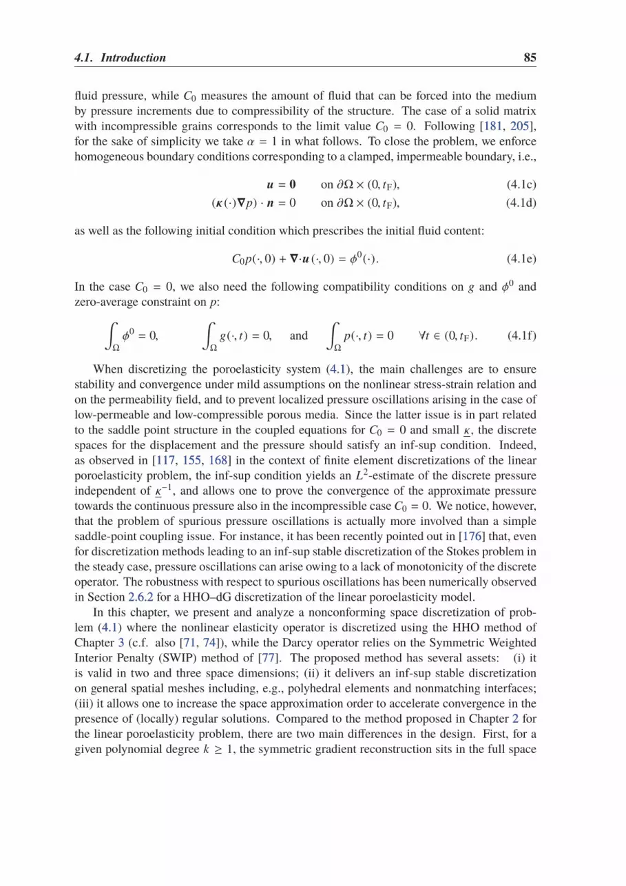
4.1. Introduction 85
fluid pressure, while C0 measures the amount of fluid that can be forced into the mediumby pressure increments due to compressibility of the structure. The case of a solid matrixwith incompressible grains corresponds to the limit value C0 = 0. Following [181181, 205205],for the sake of simplicity we take α = 1 in what follows. To close the problem, we enforcehomogeneous boundary conditions corresponding to a clamped, impermeable boundary, i.e.,
u = 0 on ∂Ω × (0, tF), (4.1c)
(κ (·)∇p) · n = 0 on ∂Ω × (0, tF), (4.1d)
as well as the following initial condition which prescribes the initial fluid content:
C0p(·, 0) + ∇·u (·, 0) = φ0(·). (4.1e)
In the case C0 = 0, we also need the following compatibility conditions on g and φ0 andzero-average constraint on p:
∫
Ω
φ0= 0,
∫
Ω
g(·, t) = 0, and
∫
Ω
p(·, t) = 0 ∀t ∈ (0, tF). (4.1f)
When discretizing the poroelasticity system (4.14.1), the main challenges are to ensurestability and convergence under mild assumptions on the nonlinear stress-strain relation andon the permeability field, and to prevent localized pressure oscillations arising in the case oflow-permeable and low-compressible porous media. Since the latter issue is in part relatedto the saddle point structure in the coupled equations for C0 = 0 and small κ , the discretespaces for the displacement and the pressure should satisfy an inf-sup condition. Indeed,as observed in [117117, 155155, 168168] in the context of finite element discretizations of the linearporoelasticity problem, the inf-sup condition yields an L2-estimate of the discrete pressureindependent of κ−1, and allows one to prove the convergence of the approximate pressuretowards the continuous pressure also in the incompressible case C0 = 0. We notice, however,that the problem of spurious pressure oscillations is actually more involved than a simplesaddle-point coupling issue. For instance, it has been recently pointed out in [176176] that, evenfor discretization methods leading to an inf-sup stable discretization of the Stokes problem inthe steady case, pressure oscillations can arise owing to a lack of monotonicity of the discreteoperator. The robustness with respect to spurious oscillations has been numerically observedin Section 2.6.22.6.2 for a HHO–dG discretization of the linear poroelasticity model.
In this chapter, we present and analyze a nonconforming space discretization of prob-lem (4.14.1) where the nonlinear elasticity operator is discretized using the HHO method ofChapter 33 (c.f. also [7171, 7474]), while the Darcy operator relies on the Symmetric WeightedInterior Penalty (SWIP) method of [7777]. The proposed method has several assets: (i) itis valid in two and three space dimensions; (ii) it delivers an inf-sup stable discretizationon general spatial meshes including, e.g., polyhedral elements and nonmatching interfaces;(iii) it allows one to increase the space approximation order to accelerate convergence in thepresence of (locally) regular solutions. Compared to the method proposed in Chapter 22 forthe linear poroelasticity problem, there are two main differences in the design. First, for agiven polynomial degree k ≥ 1, the symmetric gradient reconstruction sits in the full space

86 Chapter 4. Nonlinear poroelasticity
of tensor-valued polynomials of total degree ≤ k, as opposed to symmetric gradients ofvector-valued polynomials of total degree ≤ (k + 1). Following [3333, 7272], this modification isrequired to obtain optimal convergence rates when considering nonlinear stress-strain laws.Second, the right-hand side of the discrete problem of Section 4.4.44.4.4 is obtained by taking theaverage in time of the loading force f and fluid source g over a time step instead of their valueat the end of the time step. This modification allows us to prove stability and optimal errorestimates under significantly weaker time regularity assumptions on data (cf. Remark 4.124.12and 4.184.18). Finally, in Section 4.3.44.3.4 we give a new simple proof of discrete Korn’s inequality,not requiring particular geometrical assumption on the mesh. The interest of these resultsgoes beyond the specific application considered here.
The material is organized as follows. In Section 4.24.2 we present the assumptions on thestress-strain law and the variational formulation of the nonlinear poroelasticity problem. InSection 4.34.3 we define the space and time meshes and the discrete spaces for the displacementand the pressure fields. In Section 4.44.4 we define the discrete counterparts of the elasticity,Darcy, and hydromechanical coupling operators and formulate the discrete problem. InSection 4.54.5 we prove the well-posedness of the scheme by deriving an a priori estimateon the discrete solution that holds also when the specific storage coefficient vanishes. Theconvergence analysis of the method is carried out in Section 4.64.6.
4.2 Continuous setting
In this section we introduce the notation for function spaces, formulate the assumptions onthe stress-strain law, and derive a weak formulation of problem (4.14.1).
4.2.1 Notation for function spaces
Let X ⊂ Ω. Spaces of functions, vector fields, and tensor fields defined over X are respectivelydenoted by italic capital, boldface Roman capital, and special Roman capital letters. Thesubscript “s” appended to a special Roman capital letter denotes a space of symmetric tensorfields. Thus, for example, L2(X ),L2(X ), and L2
s (X ) denote the spaces of square integrablefunctions, vector fields, and symmetric tensor fields over X , respectively. For any measuredset X and any m ∈ Z, we denote by Hm(X ) the usual Sobolev space of functions that have weakpartial derivatives of order up to m in L2(X ), with the convention that H0(X ) ≔ L2(X ),while Cm(X ) and C∞
c (X ) denote, respectively, the usual spaces of m-times continuouslydifferentiable functions and infinitely continuously differentiable functions with compactsupport on X . We denote by (·, ·)X and (·, ·)m,X the usual scalar products in L2(X ) andHm(X ) respectively, and by ‖·‖X and ‖·‖m,X the induced norms.
For a vector space V with scalar product (·, ·)V , the space Cm(V ) ≔ Cm([0, tF]; V )
is spanned by V -valued functions that are m-times continuously differentiable in the timeinterval [0, tF]. The space Cm(V ) is a Banach space when equipped with the norm
‖ϕ‖Cm (V ) ≔ max0≤i≤m
maxt∈[0,tF]
‖ditϕ(t)‖V .
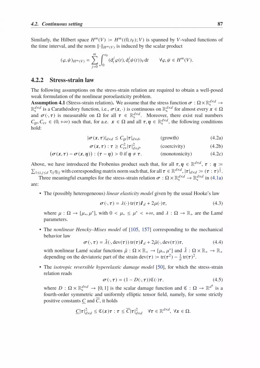
4.2. Continuous setting 87
Similarly, the Hilbert space Hm(V ) ≔ Hm((0, tF); V ) is spanned by V -valued functions ofthe time interval, and the norm ‖·‖Hm (V ) is induced by the scalar product
(ϕ, ψ)Hm (V ) =
m∑
j=0
∫ tF
0(d j
t ϕ(t), d jt ψ(t))V dt ∀ϕ, ψ ∈ Hm(V ).
4.2.2 Stress-strain law
The following assumptions on the stress-strain relation are required to obtain a well-posedweak formulation of the nonlinear poroelasticity problem.Assumption 4.1 (Stress-strain relation). We assume that the stress function σ : Ω×Rd×d
s →R
d×ds is a Carathéodory function, i.e., σ (x, ·) is continuous on Rd×d
s for almost every x ∈ Ωand σ (·, τ) is measurable on Ω for all τ ∈ Rd×d
s . Moreover, there exist real numbersCgr,Ccv ∈ (0,+∞) such that, for a.e. x ∈ Ω and all τ, η ∈ Rd×d
s , the following conditionshold:
|σ (x, τ) |d×d ≤ Cgr |τ |d×d, (growth) (4.2a)
σ (x, τ) : τ ≥ C2cv |τ |2d×d, (coercivity) (4.2b)
(
σ (x, τ) − σ (x, η))
:(
τ − η)
> 0 if η , τ. (monotonicity) (4.2c)
Above, we have introduced the Frobenius product such that, for all τ, η ∈ Rd×d , τ : η ≔∑
1≤i, j≤d τi jηi j with corresponding matrix norm such that, for all τ ∈ Rd×d , |τ |d×d ≔ (τ : τ)12 .
Three meaningful examples for the stress-strain relation σ : Ω × Rd×ds → Rd×d
s in (4.1a4.1a)are:
• The (possibly heterogeneous) linear elasticity model given by the usual Hooke’s law
σ (·, τ) = λ(·) tr(τ)I d + 2µ(·)τ, (4.3)
where µ : Ω → [µ∗, µ∗], with 0 < µ∗ ≤ µ∗ < +∞, and λ : Ω → R+ are the Laméparameters.
• The nonlinear Hencky–Mises model of [105105, 157157] corresponding to the mechanicalbehavior law
σ (·, τ) = λ(·, dev(τ)) tr(τ)I d + 2µ(·, dev(τ))τ, (4.4)
with nonlinear Lamé scalar functions µ : Ω × R+ → [µ∗, µ∗] and λ : Ω × R+ → R+depending on the deviatoric part of the strain dev(τ) ≔ tr(τ2) − 1
dtr(τ)2.
• The isotropic reversible hyperelastic damage model [5050], for which the stress-strainrelation reads
σ (·, τ) = (1 − D(·, τ))C(·)τ. (4.5)
where D : Ω × Rd×ds → [0, 1] is the scalar damage function and C : Ω → Rd4
is afourth-order symmetric and uniformly elliptic tensor field, namely, for some strictlypositive constants C and C, it holds
C |τ |2d×d ≤ C(x)τ : τ ≤ C |τ |2d×d ∀τ ∈ Rd×d, ∀x ∈ Ω.

88 Chapter 4. Nonlinear poroelasticity
Being linear, the Cauchy stress tensor in (4.34.3) clearly satisfies the previous assumptions.Moreover, under some mild requirements (cf. Appendix BB and [8787]) on the nonlinearLamé scalar functions µ and λ in (4.44.4) and on the damage function D in (4.54.5), it can beproven that also the Hencky–Mises model and the isotropic reversible damage model satisfyAssumption 4.14.1.
4.2.3 Weak formulation
At each time t ∈ [0, tF], the natural functional spaces for the displacement u (t) and porepressure p(t) taking into account the boundary condition (4.1c4.1c) and the zero average constraint(4.1f4.1f) are, respectively,
U ≔ H10(Ω) and P ≔
H1(Ω) if C0 > 0,
H1(Ω) ∩ L20(Ω) if C0 = 0,
with H10(Ω) ≔
v ∈ H1(Ω) : v |∂Ω = 0
and L2
0(Ω) ≔q ∈ L2(Ω) :
∫
Ωq = 0
. We con-
sider the following weak formulation of problem (4.14.1): For a loading term f ∈ L2(L2(Ω)),a fluid source g ∈ L2(L2(Ω)), and an initial datum φ0 ∈ L2(Ω) that verify (4.1f4.1f), findu ∈ L2(U ) and p ∈ L2(P) such that, for all v ∈ U , all q ∈ P, and all ϕ ∈ C∞
c ((0, tF))
∫ tF
0a(u (t), v ) ϕ(t)dt +
∫ tF
0b(v, p(t)) ϕ(t)dt =
∫ tF
0( f (t), v )Ω ϕ(t)dt,
(4.6a)∫ tF
0
[
b(u (t), q) − C0(p(t), q)Ω]
dtϕ(t)dt +
∫ tF
0c(p(t), q) ϕ(t)dt =
∫ tF
0(g(t), q)Ω ϕ(t)dt,
(4.6b)
(C0p(0) + ∇·u (0), q)Ω = (φ0, q)Ω, (4.6c)
where we have defined the nonlinear function a : U × U → R and the bilinear formsb : U × P → R and c : P × P → R such that, for all v, w ∈ U and all q, r ∈ P,
a(v, w ) ≔ (σ (·,∇sv ),∇sw )Ω, b(v, q) ≔ −(∇·v, q)Ω, c(q, r) ≔ (κ (·)∇r,∇q)Ω.
The first term in (4.6a4.6a) is well defined thanks to the growth assumption (4.2a4.2a). Moreover,owing to (4.2b4.2b) together with Korn’s first inequality and Poincaré’s inequality, a(·, ·) andc(·, ·) are coercive on U and P, respectively. The strict monotonicity assumption (4.2c4.2c)guarantees the uniqueness of the weak solution.
Remark 4.2 (Regularity of the fluid content and of the pore pressure). Using an integrationby parts in time in (4.6b4.6b), it is inferred that
dt
[
C0(p, q)Ω − b(u, q)]
+ c(p, q) = (g, q)Ω ∀q ∈ P in L2((0, tF)). (4.7)
Therefore, defining the fluid content φ ≔ C0p + ∇·u , we have that t 7→ (φ(t), q)Ω ∈H1((0, tF)) ⊂ C0([0, tF]) for all q ∈ P, and, as a result, (4.6c4.6c) makes sense. Moreover, in the

4.3. Discrete setting 89
case C0 > 0, taking q = 1 in (4.74.7) and owing to the definition of the bilinear form c and thehomogeneous Dirichlet condition (4.1c4.1c), we infer that
dt
(
C0
∫
Ω
p(·, t))
=
∫
Ω
g(·, t) in L2((0, tF)).
Thus, t 7→∫
Ωp(·, t) ∈ H1((0, tF)), namely the average of the pore pressure on the medium Ω
is a continuous function in [0, tF].
4.3 Discrete setting
In this section we define the space and time meshes, recall the definition and properties ofL2-orthogonal projectors on local and broken polynomial spaces, and introduce the discretespaces for the displacement and the pressure.
4.3.1 Space mesh
We consider here polygonal or polyhedral meshes corresponding to couples Mh ≔ (Th, Fh),where Th is a finite collection of polygonal elements T such that h ≔ maxT∈Th hT > 0 withhT denoting the diameter of T , while Fh is a finite collection of hyperplanar faces F. Itis assumed henceforth that the mesh Mh matches the geometrical requirements detailed in[8686, Definition 7.2]; see also [8282, Section 2]. We additionally assume here that the meshelements are star-shaped with respect to a ball of diameter uniformly comparable to theelement diameter in order to use the results of [3232, Appendix A]. To avoid dealing withjumps of the permeability coefficient inside elements, we additionally assume that Mh iscompliant with the partition PΩ on which κ is piecewise constant meaning that, for everyT ∈ Th, there exists a unique subdomain ω ∈ PΩ such that T ⊂ ω. For every mesh elementT ∈ Th, we denote by FT the subset of Fh containing the faces that lie on the boundary ∂T
of T . For each face F ∈ FT , nTF is the (constant) unit normal vector to F pointing out of T .Boundary faces lying on ∂Ω and internal faces contained in Ω are collected in the sets F b
h
and F ih, respectively.
Our focus is on the so-called h-convergence analysis, so we consider a sequence of refinedmeshes that is regular in the sense of [8282, Definition 3]. The corresponding strictly positiveregularity parameter, uniformly bounded away from zero, is denoted by . We additionallyassume that, for each mesh in the sequence, all the elements are star-shaped with respect toevery point of a ball of radius uniformly comparable to the diameter of the element. Themesh regularity assumption implies, in particular, that the diameter hT of a mesh elementT ∈ Th is uniformly comparable to the diameter hF of each face F ∈ FT , and that the numberof faces in FT is bounded above by an integer N∂ independent of h.
4.3.2 Time mesh
We subdivide (0, tF) into N ∈ N∗ uniform subintervals, and introduce the timestep τ ≔ tF/N
and the discrete times tn≔ nτ for all 0 ≤ n ≤ N . We define the space of piecewise H1

90 Chapter 4. Nonlinear poroelasticity
functions on (0, tF) by
H1(Tτ) ≔ϕ ∈ L2((0, tF)) : ϕ|(tn,tn−1) ∈ H1((tn−1, tn)) for all 1 ≤ n ≤ N
.
Since each ψ ∈ H1((tn−1, tn)) has an absolutely continuous representative in [tn−1, tn], wecan identify ϕ ∈ H1(Tτ) with a left continuous function in (0, tF). Therefore, for any vectorspace V and any ϕ ∈ H1(Tτ; V ), we set ϕ0
≔ ϕ(0) and, for all 1 ≤ n ≤ N ,
ϕn≔ lim
t→(tn )−ϕ(t) ∈ V .
If ϕ ∈ C0(V ), this simply amounts to setting ϕn≔ ϕ(tn). For all n ≥ 1 and ψ ∈ L1(V ), we
define the time average of ψ in (tn−1, tn) as
ψn≔ τ−1
∫ tn
tn−1ψ(t)dt ∈ V, (4.8)
with the convention thatψ0= 0 ∈ V . We also let, for all (ϕi)0≤i≤N ∈ V N+1 and all 1 ≤ n ≤ N ,
δtϕn≔
ϕn − ϕn−1
τ∈ V
denote the backward approximation of the first derivative of ϕ at time tn.We note a preliminary result that will be used in the convergence analysis of Section 4.64.6.
Let ψ ∈ H1(Tτ) and 1 ≤ n ≤ N . Identifying ψ|(tn−1,tn ) ∈ H1((tn−1, tn)) with its absolutelycontinuous representative in (tn−1, tn], one can use the fundamental theorem of calculus toinfer that
ψn−ψn= ψ(tn)−1
τ
∫ tn
tn−1
(
ψ(tn) −∫ tn
s
dtψ(t)dt
)
ds =1
τ
∫ tn
tn−1
∫ tn
s
dtψ(t)dt ds ≤∫ tn
tn−1|dtψ(t) |dt .
Thus, applying the previous result together with the Jensen inequality yields, for all ϕ ∈H1(Tτ; L2(Ω)),
‖ϕn − ϕn‖2Ω ≤
∫
Ω
(∫ tn
tn−1|dtϕ(x, t) |dt
)2
dx ≤ τ
∫ tn
tn−1‖dtϕ(t)‖2
Ωdt ≤ τ‖ϕ‖2H1((tn−1,tn );L2(Ω))
,
(4.9)where ϕ(x, t) is a shorthand notation for (ϕ(t))(x). As a result of (4.94.9), we get
N∑
n=1
τ‖ϕn − ϕn‖2Ω ≤ τ2
N∑
n=1
‖ϕ‖2H1((tn−1,tn );L2(Ω))
≕ τ2‖ϕ‖2H1(Tτ ;L2(Ω))
.
4.3.3 L2-orthogonal projectors on local and broken polynomial spaces
For X ⊂ Ω and k ∈ N, we denote by Pk (X ) the space spanned by the restriction to X of scalar-valued, d-variate polynomials of total degree k. The L2-projector πk
X: L1(X ) → Pk (X ) is
defined such that, for all v ∈ L1(X ),∫
X
(πkXv − v)w = 0 ∀w ∈ Pk (X ). (4.10)

4.3. Discrete setting 91
As a projector, πkX
is linear and idempotent so that, for all v ∈ Pk (X ), πkXv = v. When dealing
with the vector-valued polynomial space Pk (X ) or with the tensor-valued polynomial spaceP
k (X ), we use the boldface notation πkX
for the corresponding L2-orthogonal projectors actingcomponent-wise. At the global level, we denote by Pk (Th), Pk (Th), and Pk (Th), respectively,the spaces of fully discontinuous scalar-valued, vector-valued, and tensor-valued brokenpolynomial functions on Th of total degree k, and by πk
hand πk
hthe L2-projectors on Pk (Th)
and Pk (Th). The following optimal approximation properties for the L2-projector πkX
followfrom [6969, Lemmas 3.4 and 3.6]: There exists a strictly positive real number Cap independentof h such that, for all T ∈ Th, all l ∈ 1, . . . , k + 1, and all v ∈ H l (T ),
|v − πkTv |Hm (T ) + h
12T|v − πk
Tv |Hm (FT ) ≤ Caphl−mT |v |H l (T ) ∀m ∈ 0, . . . , l, (4.11)
where |·|Hm (FT ) is the broken Sobolev seminorm on FT .
4.3.4 Discrete spaces
In this section we define the discrete spaces upon which the HHO method corresponding toa polynomial degree k ≥ 1 is built.
4.3.4.1 Displacement
The discrete unknowns for the displacement are collected in the space
U kh≔
v
h=
(
(vT )T∈Th, (vF )F∈Fh)
: vT ∈ Pk (T ) ∀T ∈ Th and vF ∈ Pk (F) ∀F ∈ Fh
.
For any vh∈ U k
h, we denote by vh ∈ Pk (Th) the broken polynomial vector field obtained
patching element-based unknowns, so that
(vh)|T = vT ∀T ∈ Th.
The discrete unknowns corresponding to a function v ∈ H1(Ω) are obtained by means of theinterpolator I k
h: H1(Ω) → U k
hsuch that
I khv ≔
(
(πkT v |T )T∈Th, (π
kFv |F )F∈Fh
)
. (4.12)
For all T ∈ Th, we denote by U kT
and I kT
the restrictions to T of U kh
and I kh, respectively and,
for any vh∈ U k
h, we let v
T≔
(
vT, (vF )F∈FT)
collect the local discrete unknowns attached toT . At each time step, the displacement is sought in the following subspace of U k
hthat strongly
accounts for the homogeneous Dirichlet condition (4.1c4.1c):
U kh,D ≔
v
h=
(
(vT )T∈Th, (vF )F∈Fh) ∈ U k
h: vF = 0 ∀F ∈ F b
h
.
We next prove a discrete version of Korn’s first inequality on U kh,D that will play a key role
in the analysis. To this purpose, we endow the space U kh
with the discrete strain seminorm‖·‖ε,h defined, for all v
h∈ U k
h, such that
‖vh‖ε,h ≔
∑
T∈Th
*.,‖∇svT ‖2T +
∑
F∈FT
‖vF − vT ‖2F
hF
+/-
12
. (4.13)
92 Chapter 4. Nonlinear poroelasticity
We will also need the following continuous trace inequality, whose proof follows the argu-ments of [7676, Lemma 1.49] (where a slightly different notion of mesh faces is considered):There exists a strictly positive real number Ctr, independent of h but possibly depending on, such that, for all T ∈ Th, all vT ∈ H1(T ), and all F ∈ FT ,
‖vT ‖2F ≤ C2
tr
(
‖∇vT ‖T + h−1T ‖vT ‖T
)
‖vT ‖T . (4.14)
Proposition 4.3 (Discrete Korn’s first inequality). There is a real number CK > 0, only
depending on Ω, d, and such that, for all vh∈ U k
h,D,
‖vh‖Ω ≤ CK‖vh‖ε,h. (4.15)
Remark 4.4 (Strain norm). An immediate consequence of (4.154.15) is that the map ‖·‖ε,h is anorm in U k
h,D.
Proof. Let vh∈ U k
h,D. Since the divergence operator ∇· : H1s (Ω) → L2(Ω) is onto (c.f. [3131,
5656]), there exists τvh ∈ H1s (Ω) such that ∇·τvh = vh and ‖τvh ‖1,Ω ≤ Csj‖vh‖Ω, with Csj > 0
independent of h. It follows that
‖vh‖2Ω = (vh,∇·τvh )Ω =
∑
T∈Th
*.,−∫
T
∇svT : τvh +∑
F∈FT
∫
F
(vT − vF ) · τvhnTF+/- ,
where we have integrated by parts element by element and used the fact that τvh has continuousnormal components across interfaces and that boundary unknowns are set to zero in order toinsert vF into the boundary term. Applying a Cauchy–Schwarz inequality on the integralsover the element, a generalized Hölder inequality with exponents (2, 2,+∞) on the integralsover faces, using the fact that ‖nTF ‖L∞(F) ≤ 1, and invoking a discrete Cauchy–Schwarzinequality on the sum over T ∈ Th, we infer that
‖vh‖2Ω ≤
∑
T∈Th
*.,‖∇svT ‖T ‖τvh ‖T +∑
F∈FT
‖vF − vT ‖F
h12F
h12F‖τvh ‖F
+/-≤ *.,
∑
T∈Th‖∇svT ‖2
T+/-
12
‖τvh ‖Ω +*.,∑
T∈Th
∑
F∈FT
‖vF − vT ‖2F
hF
+/-12 *.,
∑
T∈Th
∑
F∈FThF ‖τvh ‖2
F+/-
12
≤√
2N∂Ctr*.,∑
T∈Th‖∇sv ‖2
T +
∑
T∈Th
∑
F∈FT
‖vF − vT ‖2F
hF
+/-12
‖τvh ‖1,Ω
=
√
2N∂Ctr‖vh‖ε,h‖τvh ‖1,Ω,
where, to pass to the third line, we have estimated ‖τvh ‖F using the continuous trace inequality(4.144.14) together with the fact that hF ≤ hT ≤ diam(Ω) = 1 for any T ∈ Th and F ∈ FT . Thus,invoking the boundedness of the divergence operator, we get
‖vh‖2Ω ≤
√
2N∂CsjCtr‖vh‖ε,h‖vh‖Ω,
which yields the conclusion with CK =√
2N∂CsjCtr.

4.4. Discretization 93
4.3.4.2 Pore pressure
At each time step, the discrete pore pressure is sought in the space
Pkh ≔
Pk (Th) if C0 > 0,
Pk0 (Th) ≔
qh ∈ Pk (Th) :
∫
Ωqh = 0
if C0 = 0.
For any internal face F ∈ F ih, we denote by TF,1,TF,2 ∈ Th the two mesh elements that share
F as a face, that is to say F ⊂ ∂TF,1 ∩ ∂TF,2 and TF,1 , TF,2 (the ordering of the elements isarbitrary but fixed), and we set
κF,i ≔
(
κ |TF, inTF, iF
)
· nTF, iF for i ∈ 1, 2, κF ≔2κF,1κF,2
κF,1 + κF,2. (4.16)
For all qh ∈ Pkh, we denote by qT the restriction of qh to an element T ∈ Th and we define the
discrete seminorm
‖qh‖κ,h ≔ *.,∑
T∈Th‖κ 1
2∇qT ‖2T +
∑
F∈F ih
κF
hF
‖qTF,1 − qTF,2 ‖2F+/-
12
. (4.17)
The fact that in (4.174.17) boundary terms only appear on internal faces reflects the homogeneousNeumann boundary condition (4.1d4.1d).
Using the surjectivity of the divergence operator∇· : H10(Ω) → L2
0(Ω) and proceeding asin the proof of the discrete Korn inequality (4.154.15), a discrete Poincaré-Wirtinger inequalityin Pk (Th) is readily inferred, namely one has the existence of CP > 0, only depending on Ω,d, and such that, for all qh ∈ Pk (Th),
‖qh − π0Ω
qh‖Ω ≤ CPκ− 1
2 ‖qh‖κ,h.
This result ensures, in particular, that the seminorm ‖·‖κ,h defined in (4.174.17) is a norm onPk
0 (Th). For a proof of more general Sobolev inequalities on broken polynomial spaces, werefer the reader to [7575] and [7676, Section 5.1.2].
4.4 Discretization
In this section we define the discrete counterparts of the elasticity, hydro-mechanical coupling,and Darcy operators, and formulate the HHO–dG scheme for problem (4.64.6).
4.4.1 Nonlinear elasticity operator
The discretization of the nonlinear elasticity operator closely follows the one presented inSection 3.43.4. We define the local symmetric gradient reconstruction Gk
s,T : U kT→ Pk
s (T ) such
that, for a given vT=
(
vT, (vF )F∈FT) ∈ U k
T, Gk
s,T vT∈ Pk
s (T ) solves∫
T
Gks,T vT
: τ = −∫
T
vT · (∇·τ) +∑
F∈FT
∫
F
vF · (τnTF ) ∀τ ∈ Pks (T ). (4.18)

94 Chapter 4. Nonlinear poroelasticity
Existence and uniqueness of Gks,T vT
follow from the Riesz representation theorem in Pks (T )
for the L2(T )d×d-inner product. This definition is motivated by the following property.Proposition 4.5 (Commuting property for the local symmetric gradient reconstruction). For
all v ∈ H1(T ), it holds that
Gks,T I
kT v = π
kT (∇sv ). (4.19)
Remark 4.6 (Approximation properties of the local symmetric gradient reconstruction). Thecommuting property (4.194.19) combined with (4.114.11) shows that Gk
s,T IkTv optimally approximates
∇sv in Pks (T ).
Proof. We start by noticing that it holds, for all α ∈ Rd×ds and all β ∈ Rd×d , denoting by
βs ≔12 (β + βT) the symmetric part of β,
α : β = α : βs. (4.20)
For all τ ∈ Pk (T ) we can then write∫
T
Gks,T I
kT v : τ =
∫
T
Gks,T I
kT v : τs
= −∫
T
πkT v · (∇·τs) +
∑
F∈FT
∫
F
πkFv · (τsnTF )
= −∫
T
v · (∇·τs) +∑
F∈FT
∫
F
v · (τsnTF )
=
∫
T
∇v : τs =
∫
T
∇sv : τs =
∫
T
∇sv : τ =
∫
T
πkT (∇sv ) : τ,
where we have used (4.204.20) with α = Gks,T I
kTv and β = τ in the first line, the definition (4.184.18)
of the local symmetric gradient with vT= I k
Tv in the second line, and definition (4.104.10) after
observing that ∇·τs ∈ Pk−1(T ) ⊂ Pk (T ) and τsnT F ∈ Pk (F) for all F ∈ FT to remove theL2-orthogonal projectors in the third line. In the fourth line, we have used an integration byparts, then invoked (4.204.20) first with α = τs and β = ∇v , then with α = ∇sv and β = τ, andwe have used the definition (4.104.10) of πk
Tto conclude.
From Gks,T , we define the local displacement reconstruction operator r k+1
T: U k
T→
Pk+1(T ) such that, for all vT∈ U k
T,
∫
T
(∇srk+1T v
T− Gk
s,T vT) : ∇sw = 0 ∀w ∈ Pk+1(T ),
∫
T
r k+1T v
T=
∫
T
vT,
∫
T
∇×(r k+1T v
T) =
∑
F∈FT
∫
F
nTF × vF,
where ∇× denotes the curl operator and v × w the vector product of two vectors v, w ∈ Rd .Optimal approximation properties for r k+1
TI k
Thave been recently proved in [3232, Appendix A]

4.4. Discretization 95
generalizing the ones of [7474, Lemma 2]. The optimal approximation properties of r k+1T
I kT
are required to infer (4.464.46) below.The discretization of the nonlinear elasticity operator is realized by the function ah :
U kh× U k
h→ R such that, for all w
h, v
h∈ U k
h,
ah(wh, v
h) ≔
∑
T∈Th
*.,∫
T
σ (·, Gks,TuT ) : Gk
s,T vT+
∑
F∈FT
γ
hF
∫
F
∆kTFuT · ∆
kTFvT
+/- , (4.21)
where γ > 0 denotes a user-dependent parameter and we penalize in a least-square sense theface-based residual ∆k
TF: U k
T→ Pk (F) such that, for all T ∈ Th, all v
T∈ U k
T, and all F ∈ FT ,
∆kTFvT
≔ πkF (r k+1
T vT− vF ) − πk
T (r k+1T v
T− vT ).
This definition ensures that ∆kTF
vanishes whenever its argument is of the form I kTw with
w ∈ Pk+1(T ), a crucial property to obtain high-order error estimates (cf. Theorems 2.122.12,3.163.16). For further use, we note the following seminorm equivalence, which can be provedusing the arguments of [7474, Lemma 4]: For all v
h∈ U k
h,
C−2eq ‖vh
‖2ε,h ≤
∑
T∈Th
*.,‖Gks,T vT
‖2T +
∑
F∈FTh−1
F ‖∆kTFvT
‖2F+/- ≤ C2
eq‖vh‖2ε,h, (4.22)
where Ceq > 0 is independent of h, and the discrete strain seminorm ‖·‖ε,h is defined by(4.134.13). By (4.2b4.2b), this implies the coercivity of ah.
Remark 4.7 (Choice of the stabilization parameter). The constants Cgr,Ccv appearing in (4.24.2)satisfy C2
cv ≤ Cgr. Indeed, owing to (4.2b4.2b), the Cauchy–Schwarz inequality, and (4.2a4.2a), itholds for all τ ∈ Rd×d
s ,
C2cv |τ |2d×d ≤ σ (x, τ) : τ ≤ |σ (x, τ) |d×d |τ |d×d ≤ Cgr |τ |2d×d . (4.23)
Thus, we choose the stabilization parameter γ in (4.214.21) such that
γ ∈ [C2cv,Cgr]. (4.24)
For the linear elasticity model (4.34.3), we have Cgr = 2µ+ dλ and Ccv =√
2µ, so that a naturalchoice for the stabilization parameter is γ = 2µ.
4.4.2 Hydro-mechanical coupling
The hydro-mechanical coupling is realized by means of the bilinear form bh on U kh× Pk (Th)
such that, for all vh∈ U k
hand all qh ∈ Pk (Th),
bh(vh, qh) ≔
∑
T∈Th
*.,∫
T
vT · ∇qT −∑
F∈FT
∫
F
vF · qTnT F+/- , (4.25)

96 Chapter 4. Nonlinear poroelasticity
where we remind the reader that qT ≔ qh|T . It can be checked using Cauchy–Schwarzinequalities together with the definition (4.134.13) of the discrete strain seminorm and discretetrace inequalities that there exists Cbd > 0 independent of h such that
bh(vh, qh) ≤ Cbd‖vh
‖ε,h‖qh‖Ω.
Additionally, using the strongly enforced boundary condition in U kh,D, it can be proved that
bh(vh, 1) = 0, ∀v
h∈ U k
h,D. (4.26)
Finally, we note the following lemma stating that the hybrid interpolator I kh
: H1(Ω) → U kh
is a Fortin operator.Lemma 4.8 (Fortin operator). For all v ∈ H1(Ω) and all qh ∈ Pk (Th), the interpolator I k
h
satisfies
‖I khv ‖ε,h ≤ Cst |v |1,Ω, (4.27a)
bh(I khv, qh) = b(v, qh), (4.27b)
where the strictly positive real number Cst is independent of h.
Proof. (i) Proof of (4.27a4.27a). Recalling the definitions (4.134.13) of the discrete strain seminormand (4.124.12) of the global interpolator, we can write
‖I khv ‖
2ε,h =
∑
T∈Th
*.,‖∇sπkT v ‖2
T +
∑
F∈FTh−1
F ‖πkFv − πk
T v ‖2F+/-
≤∑
T∈Th
*.,2‖∇s(πkT v − v )‖2
T + 2‖∇sv ‖2T +
∑
F∈FTh−1
F ‖v − πkT v ‖2
F+/- ≤ Cst |v |1,Ω,
with Cst > 0 independent of h. To pass to the second line, we have used a triangle inequalityafter inserting ±∇sv into the first term, and we have used the linearity, idempotency, andboundedness of πk
Fto write ‖πk
Fv − πk
Tv ‖F = ‖πk
F(v − πk
Tv )‖F ≤ ‖v − πk
Tv ‖F . To conclude,
we have used (4.114.11) respectively with l = m = 1 and with l = 1 and m = 0 to bound the firstand third terms inside the summation.
(ii) Proof of (4.27b4.27b). Recalling the definitions (4.254.25) of bh(·, ·) and (4.124.12) of the globalinterpolator, we can write for all qh ∈ Pk (Th),
bh(I khv, qh) =
∑
T∈Th
(∫
T
πkT v · ∇qT −
∫
F
πkFv |F · qTnTF
)
=
∑
T∈Th
(∫
T
v · ∇qT −∫
F
v · qTnT F
)
= b(v, qh),
where we have used definition (4.104.10) after observing that ∇qT ∈ Pk−1(T ) ⊂ Pk (T ) andqT |FnTF ∈ Pk (F) to remove the L2-orthogonal projectors in the second line, and integrationby parts over T ∈ Th to conclude.

4.4. Discretization 97
As a result of the previous Lemma, one has the following inf-sup condition, cf. PropositionA.1A.1 for the proof.Proposition 4.9. There is a strictly positive real number β independent of h such that, for
all qh ∈ Pk0 (Th),
‖qh‖Ω ≤ β supvh∈Uk
h,D\0
bh(vh, qh)
‖vh‖ε,h
. (4.28)
4.4.3 Darcy operator
The discretization of the Darcy operator is based on the Symmetric Weighted Interior Penaltymethod of [7777], cf. also [7676, Section 4.5]. For all F ∈ F i
hand all qh ∈ Pk (Th), we define the
jump and weighted average operators such that
[qh]F ≔ qTF,1 − qTF,2, qhF ≔√κF,2
√κF,1 +
√κF,2
qTF,1 +
√κF,1
√κF,1 +
√κF,2
qTF,2,
with TF,1,TF,2 ∈ Th, TF,1 , TF,2, such that F ⊂ ∂TF,1 ∩ ∂TF,2 and κF,1, κF,2 defined in (4.164.16).The bilinear form ch on Pk (Th) × Pk (Th) is defined such that, for all qh, rh ∈ Pk (Th),
ch(rh, qh) ≔
∫
Ω
κ∇hrh · ∇hqh +
∑
F∈F ih
ςκF
hF
∫
F
[rh]F[qh]F
−∑
F∈F ih
∫
F
(
[rh]F κ∇hqhF + [qh]F κ∇hrhF) · nT1F,
where we have introduced the broken gradient operator ∇h on Th and we have denoted byς > ς > 0 a user-defined penalty parameter chosen large enough to ensure the coercivity ofch (the proof is similar to [7676, Lemma 4.51]):
ch(qh, qh) ≥ (ς − ς)(1 + ς)−1‖qh‖2κ,h, ∀qh ∈ Pk
h .
Since, under this condition, ch is a symmetric positive definite bilinear form on the brokenpolynomial space Pk
h, we can define an associated norm by setting ‖ · ‖c,h ≔ ch(·, ·) 1
2 .The following consistency result can be proved adapting the arguments of [7676, Chapter 4]
to homogeneous Neumann boundary conditions and will be instrumental for the analysis.We define the functional spaces P∗ ≔
r ∈ H1(Ω) ∩ H2(PΩ) : κ∇r · n = 0 on ∂Ω
and set
Pk∗h≔ P∗ + Pk
h. Extending the bilinear form ch to Pk
∗h× Pk
∗h, it is inferred that, for all r ∈ P∗,
−(∇·(κ∇r), q)Ω = ch(r, q) ∀q ∈ P∗h. (4.29)
4.4.4 Discrete problem
For all 1 ≤ n ≤ N , the discrete solution (unh, pn
h) ∈ U k
h,D × Pkh
at time tn is such that, for all
(vh, qh) ∈ U k
h,D × Pk (Th),
ah(unh, vh
) + bh(vh, pn
h) = ( fn, vh)Ω, (4.30a)
C0(δt pnh, qh)Ω − bh(δtu
nh, qh) + ch(pn
h, qh) = (gn, qh)Ω, (4.30b)

98 Chapter 4. Nonlinear poroelasticity
with fn ∈ L2(Ω) and g
n ∈ L2(Ω) defined in Section 4.3.24.3.2. In order to start the time-steppingscheme we need to initialize the discrete fluid content. This is done by setting φ0
hequal to
the L2-orthogonal projection of φ0 on Pk (Th) according to (4.6c4.6c). This implies in particularthat
C0(p0h, qh)Ω − bh(u0
h, qh) ≔ (φ0, qh)Ω ∀qh ∈ Pk (Th). (4.30c)
Remark 4.10 (Advance in time scheme). The modified backward Euler scheme obtained bytaking time averages instead of pointwise evaluation of the right-hand sides in (4.304.30) can beinterpreted as a low-order discontinuous Galerkin time-stepping method, cf. [179179, 183183].
Notice that other time discretizations could be used, but we have decided to focus on thebackward Euler scheme to keep the proofs as simple as possible. From the practical point ofview, at each time step n, the discrete nonlinear system (4.304.30) can be solved by the Newtonmethod using as initial guess the solution at step (n − 1). The size of the linear system to besolved at each Newton iteration can be reduced by statically condensing a large part of theunknowns as described in Section 2.52.5.
4.5 Stability and well-posedness
In this section we study the stability of problem (4.304.30) and prove its well-posedness. We startwith an a priori estimate on the discrete solutions not requiring conditions on the time step τand robust with respect to vanishing storage coefficients and small permeability fields.Proposition 4.11 (A priori estimate). Denote by (un
h, pn
h)1≤n≤N the solution to (4.304.30). Under
Assumption 4.14.1 on the stress-strain relation and the regularity on the data f , g, and φ0
assumed in Section 4.2.34.2.3, it holds
N∑
n=1
τ‖unh‖
2ε,h +
N∑
n=1
τ(
‖pnh − π
0Ω
pnh‖
2Ω + C0‖pn
h‖2Ω
)
+ ‖sNh ‖
2c,h ≤
C *,‖ f ‖2L2(L2(Ω))
+ t2F‖g‖2
L2(L2(Ω))+ tF‖φ0‖2
Ω +
t2F
C0‖π0Ωg‖2
L2(L2(Ω))+
tF
C0‖π0Ωφ0‖2Ω.+- .
(4.31)
where C > 0 denotes a real number independent of h, τ, the physical parameters C0 and κ ,
and the final time tF. In (4.314.31), we have defined sNh≔
∑Nn=1 τpn
hand we have adopted the
convention that C−10 ‖π0
Ωg‖2
L2(L2(Ω))= 0 and C−1
0 ‖π0Ωφ0‖2Ω= 0 if C0 = 0.
Remark 4.12. In order to prove the a priori bound (4.314.31), no additional time regularityassumption on the loading term f and the mass source g are needed, whereas the stabilityestimate of Lemma 2.72.7, valid for linear stress-strain relation, requires f ∈ C1(L2(Ω)) andg ∈ C0(L2(Ω)). On the other hand, Proposition 4.114.11 gives an estimate of the discretedisplacement and pressure in the L2-norm in time, while Lemma 2.72.7 ensures a control inthe L∞-norm in time. However, under additional requirements on the stress-strain law (forinstance Assumption 4.154.15) and H1-regularity in time of f , a stronger version of (4.314.31) canbe inferred, establishing in particular an estimate in the L∞-norm in time.

4.5. Stability and well-posedness 99
Proof. (i) Estimate of ‖pnh− π0Ω
pnh‖Ω. The growth property of the stress-strain function (4.2a4.2a)
together with the Cauchy–Schwarz inequality, assumption (4.244.24), and the second inequalityin (4.224.22) yield, for all 1 ≤ n ≤ N and all v
h∈ U k
h,D,
ah(unh, vh
) =∑
T∈Th
*.,∫
T
σ (·, Gks,Tu
nT ) : Gk
s,T vT+
∑
F∈FT
γ
hF
∫
F
∆kTFu
nT · ∆
kTFvT
+/-≤ Cgr
∑
T∈Th
*.,‖Gks,Tu
nT ‖T ‖G
ks,T vT
‖T +∑
F∈FT
1
hF
‖∆kTFu
nT ‖F ‖∆k
TFvT‖F+/-
≤ CgrC2eq‖un
h‖ε,h‖vh‖ε,h.
(4.32)
Using the inf-sup condition (4.284.28), (4.264.26), and the mechanical equilibrium equation (4.30a4.30a),we get, for any 1 ≤ n ≤ N ,
‖pnh − π
0Ω
pnh‖Ω ≤ β sup
vh∈Ukh,D\0
bh(vh, pn
h− π0Ω
pnh)
‖vh‖ε,h
= β supvh∈Uk
h,D\0
( fn, vh)Ω − ah(un
h, v
h)
‖vh‖ε,h
.
Therefore, owing to the discrete Korn inequality (4.154.15) and to (4.324.32), we infer from theprevious bound that
‖pnh − π
0Ω
pnh‖Ω ≤ β
(
CK‖ fn‖Ω + CgrC
2eq‖un
h‖ε,h)
. (4.33)
(ii) Energy balance. For all 1 ≤ n ≤ N , summing (4.30b4.30b) at times 1 ≤ i ≤ n and takingqh = τ
2pnh
as a test function yields
τC0(pnh, pn
h)Ω − τbh(unh, pn
h) +
n∑
i=1
τ2ch(pih, pn
h) =
n∑
i=1
τ2(gi, pn
h)Ω + τ(φ0, pnh)Ω. (4.34)
Moreover, using the linearity of ch and the formula 2x(x − y) = x2+ (x − y)2 − y
2, the thirdterm in the left-hand side of (4.344.34) can be rewritten as
n∑
i=1
τ2ch(pih, pn
h) = τch*,
n∑
i=1
τpih, pn
h+- = τch(sn
h, δt snh) =
1
2
(
‖snh‖
2c,h + ‖δt s
nh‖
2c,h − ‖sn−1
h ‖2c,h
)
,
where we have set s0h≔ 0, sn
h≔
∑ni=1 τpi
hfor any 1 ≤ n ≤ N , and observed that pn
h= δt s
nh.
Therefore, summing (4.344.34) and (4.30a4.30a) at discrete time n with vh= τun
h, leads to
τah(unh, u
nh)+τC0‖pn
h‖2Ω+
1
2
(
‖snh‖
2c,h − ‖sn−1
h ‖2c,h
)
≤ τ( fn, un
h)Ω+
n∑
i=1
τ2(gi, pn
h)Ω+τ(φ0, pnh)Ω.
Summing the previous relation for 1 ≤ n ≤ N , telescoping out the appropriate summands,and using the coercivity property (4.2b4.2b), assumption (4.244.24), and the first inequality in (4.224.22),we get
C2cv
C2eq
N∑
n=1
τ‖unh‖
2ε,h+C0
N∑
n=1
τ‖pnh‖
2Ω+
1
2‖sN
h ‖2c,h ≤
N∑
n=1
τ( fn, un
h)Ω+
N∑
n=1
τ(Gn+φ0, pn
h)Ω, (4.35)

100 Chapter 4. Nonlinear poroelasticity
with the notation Gn≔
∑ni=1 τg
i=
∫ tn
0g(t)dt. We denote by R the right-hand side of (4.354.35)
and proceed to find a suitable upper bound.
(iii) Upper bound for R. For the first term in the right-hand side of (4.354.35), using theCauchy–Schwarz, discrete Korn (4.154.15), and Young inequalities, we obtain
N∑
n=1
τ( fn, un
h)Ω ≤ CK*,
N∑
n=1
τ‖ f n‖2Ω+-
12 *,
N∑
n=1
τ‖unh‖
2ε,h
+-12
≤C2
KC2eq
C2cv
‖ f ‖2L2(L2(Ω))
+
C2cv
4C2eq
N∑
n=1
τ‖unh‖
2ε,h,
(4.36)
where we have used the Jensen inequality to infer that
N∑
n=1
τ‖ f n‖2Ω =
N∑
n=1
1
τ
∫
Ω
(∫ tn
tn−1f (x, t)dt
)2
dx ≤N
∑
n=1
∫ tn
tn−1‖ f (t)‖2
Ωdt = ‖ f ‖2L2(L2(Ω))
.
We estimate the second term in the right-hand side of (4.354.35) by splitting it into two contribu-tions as follows:
N∑
n=1
τ(Gn+ φ0, pn
h)Ω =
N∑
n=1
τ(Gn+ φ0, pn
h − π0Ω
pnh)Ω +
N∑
n=1
τ(π0Ω
(Gn+ φ0), pn
h)Ω ≔ T1 + T2,
where we have used its definition (4.104.10) to move π0Ω
from pnh
to (Gn+ φ0) in the second term.
Owing to the Cauchy–Schwarz, triangle, Jensen, and Young inequalities, and using (4.334.33),we have
|T1 | ≤ *,N
∑
n=1
τ‖Gn+ φ0‖2
Ω+-
12 *,
N∑
n=1
τ‖pnh − π
0Ω
pnh‖
2Ω+-
12
≤√
2β *,N
∑
n=1
τ
∫
Ω
(∫ tn
0g(x, t)dt
)2
dx + tF‖φ0‖2Ω+-
12 *,
N∑
n=1
τ(
CK‖ fn‖Ω + CgrC
2eq‖un
h‖ε,h)2+-
12
≤ 2β(
tF‖g‖L2(L2(Ω)) + t12F ‖φ
0‖Ω)
CK‖ f ‖L2(L2(Ω)) + CgrC
2eq*,
N∑
n=1
τ‖unh‖
2ε,h
+-12
≤ tF β2 *,1 +
C2grC
6eq
C2cv
+-(
t12F ‖g‖L2(L2(Ω)) + ‖φ0‖Ω
)2
+ C2K‖ f ‖2
L2(L2(Ω))+
C2cv
4C2eq
N∑
n=1
τ‖unh‖
2ε,h.
(4.37)Owing to the compatibility condition (4.1f4.1f) and the linearity of the L2-projector, T2 =
0 if C0 = 0. Otherwise, using again the Cauchy–Schwarz, triangle, Jensen, and Young

4.5. Stability and well-posedness 101
inequalities, leads to
|T2 | ≤ *,N
∑
n=1
τ‖π0Ω
Gn+ π0Ωφ0‖2Ω+-
12 *,
N∑
n=1
τ‖pnh‖
2Ω+-
12
≤√
2(
t2F‖π0
Ωg‖2
L2(L2(Ω))+ tF‖π0
Ωφ0‖2Ω
)12 *,
N∑
n=1
τ‖pnh‖
2Ω+-
12
≤2t2
F
3C0‖π0Ωg‖2
L2(L2(Ω))+
2tF
3C0‖π0Ωφ0‖2Ω +
3C0
4
N∑
n=1
τ‖pnh‖
2Ω.
(4.38)
Finally, from (4.364.36), (4.374.37), (4.384.38), it follows that
R ≤ C2cv
2C2eq
N∑
n=1
τ‖unh‖
2ε,h +
3C0
4
N∑
n=1
τ‖pnh‖
2Ω +
2t2F
3C0‖π0Ωg‖2
L2(L2(Ω))+
2tF
3C0‖π0Ωφ0‖2Ω
+
C2K
C2cv
(
C2eq + C2
cv
)
‖ f ‖2L2(L2(Ω))
+
tF β2
C2cv
(
4C2grC
6eq + C2
cv
)
(
t12F ‖g‖L2(L2(Ω)) + ‖φ0‖Ω
)2
.
(4.39)
(iv) Conclusion. Passing the first two terms in the right-hand side of (4.394.39) to the left-handside of (4.354.35) and multiplying both sides by a factor 4, we obtain
2C2cv
C2eq
N∑
n=1
τ‖unh‖
2ε,h + C0
N∑
n=1
τ‖pnh‖
2Ω + 2‖sN
h ‖2c,h ≤ 4C, (4.40)
where we have denoted by C the last four summands in the right-hand side of (4.394.39). Inorder to conclude we apply again (4.334.33) to obtain a bound of the L2-norm of the discretepressure independent of the storage coefficient C0. Indeed, owing to (4.334.33) and C2
cv ≤ Cgr, itis inferred that
C2cv
2C2grC
6eq
N∑
n=1
τ‖pnh − π
0Ω
pnh‖
2Ω ≤
C2cv
C2eq
N∑
n=1
τ‖unh‖
2ε,h +
β2C2K
C2cvC6
eq
‖ f ‖2L2(L2(Ω))
.
Summing the previous relation to (4.404.40) yields
C2cv
C2eq
N∑
n=1
τ‖unh‖
2ε,h +
C2cv
2C2grC
6eq
N∑
n=1
τ‖pnh − π
0Ω
pnh‖
2Ω + C0
N∑
n=1
τ‖pnh‖
2Ω + 2‖sN
h ‖2c,h ≤
8t2F
3C0‖π0Ωg‖2
L2(L2(Ω))+
8tF
3C0‖π0Ωφ0‖2Ω + C2
K*,4C2
eq
C2cv
+
β2
C6eqC2
cv
+ 4+- ‖ f ‖2L2(L2(Ω))
+ 4tF β2 *,
4C2grC
6eq
C2cv
+ 1+- (t12F ‖g‖L2(L2(Ω)) + ‖φ0‖Ω)2.
Thus, multiplying both sides of the previous relation by maxC2eqC−2
cv , 2C2grC
6eqC−2
cv , 1 gives(4.314.31).

102 Chapter 4. Nonlinear poroelasticity
Remark 4.13 (A priori bound for C0 = 0). When C0 = 0, the a priori bound (4.314.31) reads
N∑
n=1
τ‖unh‖
2ε,h +
N∑
n=1
τ‖pnh‖
2Ω + ‖sN
h ‖2c,h ≤ C
(
‖ f ‖2L2(L2(Ω))
+ t2F‖g‖2
L2(L2(Ω))+ tF‖φ0‖2
Ω
)
.
The conventions C−10 ‖π0
Ωg‖2
L2(L2(Ω))= 0 and C−1
0 ‖π0Ωφ0‖2Ω= 0 if C0 = 0 are justified since
the term T2 in point (3) of the previous proof vanishes in this case thanks to the compatibilitycondition (4.1f4.1f).
We next proceed to discuss the existence and uniqueness of the discrete solutions. Theproof of the following theorem hinges on the arguments of [6464, Theorem 3.3].Theorem 4.14 (Existence and uniqueness). Let Assumption 4.14.1 hold and let (Mh)h∈H be a
regular mesh sequence. Then, for all h ∈ H and all N ∈ N∗, there exists a unique solution
(unh, pn
h)1≤n≤N ∈ (U k
h,D × Pkh
)N to (4.304.30).
Proof. We define the linear stress-strain function σ lin : Rd×ds → R
d×ds such that, for all
τ ∈ Rd×ds ,
σ lin(τ) =C2
cv
2τ +
C2cv
2dtr(τ)I d,
where Ccv is the coercivity constant of σ (see (4.2b4.2b)), and we denote by alinh
the bilinearform obtained by replacing σ with σ lin in (4.214.21). We consider the following auxiliary linearproblem:c4: For all 1 ≤ n ≤ N , find (yn
h, pn
h) ∈ U k
h,D × Pkh
such that
alinh (yn
h, v
h) + bh(v
h, pn
h) = ( fn, vh)Ω ∀v
h∈ U k
h,D,
C0(δt pnh, qh)Ω − bh(δt y
n
h, qh) + ch(pn
h, qh) = (gn, qh)Ω ∀qh ∈ Pk
h,(4.41)
with initial condition as in (4.30c4.30c). Since the previous system is linear and square and itssolution satisfies the a priori estimate of Proposition 4.114.11, it is readily inferred that problem(4.414.41) admits a unique solution.
Now we observe that, thanks to the norm equivalence (4.224.22), alinh
(·, ·) is a scalar producton U k
h,D, and we define the mapping Φ : U kh,D → U k
h,D such that, for all vh∈ U k
h,D,
alinh (Φ(v
h), w
h) = ah(v
h, w
h), ∀w
h∈ U k
h,D.
We want to show that Φ is an isomorphism. Let vh, z
h∈ U k
h,D be such that Φ(vh) = Φ(z
h).
If vh, z
h, owing to the norm equivalence (4.224.22) and the fact that ‖ · ‖ε,h is a norm on U k
h,D,
there is at least one T ∈ Th such that Gks,T vT
, Gks,T zT
or ∆kTF
vT, ∆k
TFz
Tfor some F ∈ FT .
In both cases, owing to the definition of ah and the strict monotonicity assumption (4.2c4.2c), itholds
0 < ah(vh, v
h− z
h) − ah(z
h, v
h− z
h) = alin
h (Φ(vh) − Φ(z
h), v
h− z
h) = 0.
Thus, we infer by contradiction that vh= z
hand, as a result, Φ is injective. In order to
prove that Φ is also onto, we recall the following result: If (E, (·, ·)E ) is a Euclidean space

4.6. Convergence analysis 103
and Ψ : E → E is a continuous map such that (Ψ(x),x)E‖x‖E → +∞ as ‖x‖E → +∞, then Ψ is
surjective. Since (U kh,D, alin
h(·, ·)) is a Euclidean space and the coercivity (4.2b4.2b) of σ together
with the definition of σlin yields alinh
(Φ(vh), v
h) ≥ alin
h(v
h, v
h) for all v
h∈ U k
h,D, we deduce
thatΦ is an isomorphism. Let, for all 1 ≤ n ≤ N , (yn
h, pn
h) ∈ U k
h,D×Pkh
be the unique solutionto problem (4.414.41). By the surjectivity and injectivity of Φ, for all 1 ≤ n ≤ N , there exists aunique un
h∈ U k
h,D such that Φ(unh) = yn
h. By definition of Φ and (yn
h)1≤n≤N , (un
h, pn
h)1≤n≤N
is therefore the unique solution of the discrete problem (4.304.30).
4.6 Convergence analysis
In this section we study the convergence of problem (4.304.30) and prove optimal error estimatesunder the following additional assumptions on the stress-strain function σ .Assumption 4.15 (Stress-strain relation II). There exist real numbers Clp,Cmn ∈ (0,+∞)
such that, for a.e. x ∈ Ω, and all τ, η ∈ Rd×ds ,
|σ (x, τ) − σ (x, η) |d×d ≤ Clp |τ − η |d×d, (Lipschitz continuity) (4.42a)(
σ (x, τ) − σ (x, η))
:(
τ − η) ≥ C2mn |τ − η |2d×d . (strong monotonicity) (4.42b)
Remark 4.16 (Lipschitz continuity and strong monotonocity). It is readily seen, by takingη = 0 in (4.424.42), that Lipschitz continuity and strong monotonicity imply respectively thegrowth and coercivity properties of Assumption 4.14.1. Therefore, recalling (4.234.23), it is inferredthat the constants appearing in (4.2a4.2a), (4.2b4.2b), (4.42a4.42a), and (4.42b4.42b) satisfy
C2mn ≤ C2
cv ≤ Cgr ≤ Clp. (4.43)
It was proved in [1313, Lemma 4.1] that the stress-strain relation for the Hencky–Mises modelis strongly monotone and Lipschitz-continuous. Also the isotropic damage model satisfiesAssumption 4.154.15 if the damage function in (4.54.5) is, for instance, such that
D(x, |τ |) = 1 − (1 + |C(x)τ |d×d)−12 ∀x ∈ Ω.
In order to prove a convergence rate of (k + 1) in space for both the displacement andpressure errors, we assume from this point on that the permeability tensor field κ is constanton Ω, and that the following elliptic regularity holds (which is the case, e.g., when Ω isconvex [115115, 149149]): There is a real number Cel > 0 only depending on Ω such that, for allψ ∈ L2
0(Ω), the unique function ζ ∈ P solution of the homogeneous Neumann problem
−∇·(κ∇ζ ) = ψ in Ω, κ∇ζ · n = 0 on ∂Ω,
is such that‖ζ ‖H2(Ω) ≤ Celκ
− 12 ‖ψ‖Ω. (4.44)
Let (unh, pn
h)1≤n≤N be the solution to (4.304.30). We consider, for all 1 ≤ n ≤ N , the discrete
error components defined as
enh≔ un
h − I khu
n, ǫnh ≔ pn
h − pnh, (4.45)
104 Chapter 4. Nonlinear poroelasticity
where the global elliptic projection pnh∈ Pk
his defined as the solution to
ch(pnh, qh) = ch(pn, qh) ∀qh ∈ Pk
h and
∫
Ω
pnh =
∫
Ω
pn.
Before proving the convergence of the scheme, we recall two preliminary approximationresults for the projector I k
hand the projection pn
hthat have been proved in [3333, Theorem 16]
and [3030, Lemma 11], respectively. There is a strictly positive constant Cpj depending only onΩ, k, and the mesh regularity parameter, such that,
• Assuming (4.424.42) and u ∈ L2(U ∩Hk+2(Th)) with σ (·,∇su ) ∈ L2(Hk+1s (Th)), for a.e.
t ∈ (0, tF) and all vh∈ U k
h,D, it holds
ah(I khu (·, t), v
h) + (∇·σ (·,∇su (·, t)), vh)
≤Cpjh
k+1(
|u (·, t) |Hk+2(Th ) + |σ (·,∇su (·, t)) |Hk+1(Th )
)
‖vh‖ε,h. (4.46)
• Assuming the elliptic regularity (4.444.44) and pn ∈ P ∩ H k+1(Th), for all 1 ≤ n ≤ N , itholds
h‖ pnh − pn‖c,h + κ
12 ‖ pn
h − pn‖Ω ≤ Cpjhk+1κ
12 |pn |Hk+1(Th ) . (4.47)
Now we have all the ingredients to estimate the discrete errors defined in (4.454.45).Theorem 4.17 (Error estimate). Let (u, p) denote the unique solution to (4.64.6), for which we
assumeu ∈ H1(Tτ;U ) ∩ L2(Hk+2(Th)), σ (·,∇su ) ∈ L2(Hk+1
s (Th)),
p ∈ L2(P ∩ H k+1(Th)), φ ∈ H1(Tτ; L2(Ω)),
with φ = C0p + ∇·u . If C0 > 0, we further assume π0Ω
p ∈ H1(Tτ; P0(Ω)) ≕ H1(Tτ). Then,
under Assumption 4.154.15 and the elliptic regularity (4.444.44), it holds
N∑
n=1
τ‖enh‖2ε,h +
N∑
n=1
τ(
‖ǫnh − π
0Ωǫn
h‖2Ω + C0‖ǫn
h‖2Ω
)
+ ‖zNh ‖
2c,h ≤ C
(
h2k+2C1 + τ2C2
)
, (4.48)
where C is a strictly positive constant independent of h, τ, C0, κ , and tF, and, for the sake of
brevity, we have defined zNh≔
∑Nn=1 τǫ
nh
and introduced the bounded quantities
C1 ≔ |u |2L2(Hk+2(Th ))
+ |σ (·,∇su ) |2L2(Hk+1(Th ))
+ (1 + C0)κ
κ|p|2
L2(Hk+1(Th )),
C2 ≔ ‖u ‖2H1(Tτ ;H1(Ω))
+ ‖φ‖2H1(Tτ ;L2(Ω))
+ C0‖π0Ω
p‖2H1(Tτ )
.
Remark 4.18 (Time regularity). In order to prove the previous error estimate, we only requirethe displacement u and the fluid content φ solving problem (4.64.6) to be piecewise H1-regularin (0, tF), whereas 2.122.12 is established under the much stronger regularity u ∈ C2(H1(Ω))
and, if C0 > 0, p ∈ C2(L2(Ω)). Moreover, the assumptions φ ∈ H1(Tτ; L2(Ω)) and, ifC0 > 0, π0
Ωp ∈ H1(Tτ) are consistent with the time regularity results observed in Remark
4.24.2.

4.6. Convergence analysis 105
Proof. (i) Estimate of ‖enh‖2ε,h
. First we observe that, owing to (4.1a4.1a) and the definition of bh
given in (4.254.25), for all vh∈ U k
h,D and all 1 ≤ n ≤ N , we have
( fn, vh)Ω = −(∇·σn
(·,∇su ), vh)Ω + (∇pn, vh)Ω = ah(I khu
n, vh) + bh(v
h, pn
h) − Rn(vh),
(4.49)where the residual linear form Rn : U k
h,D → R is defined such that, for all vh∈ U k
h,D,
Rn(vh) ≔ ah(I k
hun, v
h) + (∇·σn
(·,∇su ), vh)Ω,+bh(vh, pn
h) − (∇pn, vh)Ω. (4.50)
Using the norm equivalence (4.224.22), the strong monotonicity (4.42b4.42b) of σ along with as-sumption (4.244.24) on the stabilization parameter, the discrete mechanical equilibrium (4.30a4.30a),and (4.494.49), yields
C2mn
C2eq
‖enh‖2ε,h = C2
mn
∑
T∈Th
*.,‖Gks,T e
nT‖2
T +
∑
F∈FT
1
hF
‖∆kTF e
nT‖2
F+/-
≤ ah(unh, e
nh) − ah(I k
hun, en
h)
= ( fn, en
h)Ω − bh(enh, pn
h) − ah(I khu
n, enh) = −bh(en
h, ǫn
h) − Rn(enh).
Thus, owing to the previous relation and defining the dual norm
‖Rn‖ε,h,∗ ≔ supvh∈Uk
h,D\0
Rn(vnh)
‖vnh‖ε,h
,
we have that
C2mn
C2eq
‖enh‖2ε,h + bh(en
h, ǫn
h) ≤ ‖Rn‖ε,h,∗‖enh‖ε,h ≤
C2eq
2C2mn
‖Rn‖2ε,h,∗ +
C2mn
2C2eq
‖enh‖2ε,h,
where the conclusion follows from Young’s inequality. Hence, rearranging, we arrive at
C2mn
2C2eq
‖enh‖2ε,h + bh(en
h, ǫn
h) ≤C2
eq
2C2mn
‖Rn‖2ε,h,∗ (4.51)
(ii) Estimate of C0‖ǫnh‖2Ω
. Using (4.1b4.1b), the fact that (∇·u(t), 1)Ω = 0 to insert π0Ω
qh, and theconsistency property (4.294.29), we infer that, for all qh ∈ Pk
hand all 1 ≤ i ≤ N ,
(gi, qh)Ω = (C0dt p
i, qh)Ω + (∇·(dtui), qh − π0
Ωqh)Ω − (∇·(κ∇pi
), qh)Ω
= τ−1∫ t i
t i−1dt
[C0(p(t), qh)Ω + (∇·u (t), qh − π0
Ωqh)Ω
]dt + ch(pi, qh)
= δt
[C0(pi, qh)Ω + (∇·ui, qh − π0
Ωqh)Ω
]+ ch(pi, qh).
(4.52)

106 Chapter 4. Nonlinear poroelasticity
Therefore, using the discrete mass conservation equation (4.30b4.30b), (4.264.26), the Fortin property(4.27b4.27b) , the definition of the elliptic projection pn
h, and (4.524.52), we obtain
C0(δtǫih, qh)Ω − bh(δt e
ih, qh) + ch(ǫ i
h, qh)
= (gi, qh)Ω − C0(δt p
ih, qh)Ω + bh(δt (I
khu
i), qh − π0
Ωqh) − ch(pi
h, qh)
= (gi, qh)Ω − δt
[C0(pi
h, qh)Ω − (∇·ui, qh − π0Ω
qh)Ω
]− ch(pi, qh)
= δt
[C0(pi − pi
h, qh)Ω + (∇·ui − ∇·ui, qh − π0Ω
qh)Ω
]= δt
[C0(pi − pi
h, qh)Ω + C0(π0Ω
(pi − pi), qh)Ω + (φi − φi
, qh − π0Ω
qh)Ω
],
(4.53)where, in order to pass to the last line, we have inserted ±pi into the first term inside bracketsin the third line, we have defined, according to (4.1e4.1e), φi
≔ C0pi+ ∇·ui for all 0 ≤ i ≤ N ,
and we have used the definition of the global L2-projector π0Ω
. Moreover, setting p0h≔ 0, it
follows from the initial condition (4.30c4.30c), the boundary condition (4.1c4.1c), and (4.264.26) that
C0(ǫ0h, qh)Ω − bh(e0
h, qh) = (φ0, qh)Ω = (φ0, qh − π0
Ωqh)Ω + C0(π0
Ωp0, qh)Ω. (4.54)
For all 1 ≤ n ≤ N , summing (4.534.53) for 1 ≤ i ≤ n with the choice qh = τǫnh, using (4.544.54), and
proceeding as in the second step of the proof of Proposition 4.114.11, leads to
C0‖ǫnh‖
2Ω − bh(en
h, ǫn
h) +1
2τ
(
‖znh‖
2c,h − ‖zn−1
h ‖2c,h
)
≤ C0(pn − pnh, ǫ
nh)Ω + C0(π0
Ω(pn − pn
), ǫnh)Ω + (φn − φn
, ǫnh − π
0Ωǫn
h)Ω, (4.55)
where znh≔
∑ni=1 τǫ
ih
if n ≥ 1 and z0h≔ 0. We bound the first term in the right-hand side of
(4.554.55) applying the Cauchy–Schwarz and Young inequalities followed by the approximationresult (4.474.47), yielding
C0(pn − pnh, ǫ
nh)Ω ≤ C2
pjh2(k+1) κ
κC0 |pn |2
Hk+1(Th )+
C0
4‖ǫn
h‖2Ω
≤ C2pj
h2(k+1)
τ
(
κ
κ
)
C0 |p|2L2((tn−1,tn );Hk+1(Th ))+
C0
4‖ǫn
h‖2Ω,
(4.56)
where, in order to pass to the second line, we have used the Cauchy–Schwarz inequalityand adopted the notation | · |L2((tn−1,tn );Hm (Th )) ≔ ‖| · |Hm (Th ) ‖L2((tn−1,tn )), for any m ∈ N. Weestimate the second and third terms using the Cauchy–Schwarz and the Young inequalitiestogether with the time approximation result (4.94.9) as follows:
C0(π0Ω
(pn − pn), ǫn
h)Ω ≤ C0τ‖π0Ω
p‖2H1((tn−1,tn ))
+
C0
4‖ǫn
h‖2Ω,
(φn − φn, ǫn
h − π0Ωǫn
h)Ω ≤ ητ‖φ‖2H1((tn−1,tn );L2(Ω))
+
1
4η‖ǫn
h − π0Ωǫn
h‖2Ω,
(4.57)

4.6. Convergence analysis 107
with η denoting a positive real number that will be fixed later on in the proof. The relationobtained by plugging (4.564.56) and (4.574.57) into (4.554.55) reads
C0
2‖ǫn
h‖2Ω − bh(en
h, ǫn
h) +1
2τ
(
‖znh‖
2c,h − ‖zn−1
h ‖2c,h
)
− 1
4η‖ǫn
h − π0Ωǫn
h‖2Ω ≤
C2pj
h2(k+1)
τ
(
κ
κ
)
C0 |p|2L2((tn−1,tn );Hk+1(Th ))+ C0τ‖π0
Ωp‖2
H1((tn−1,tn ))+ ητ‖φ‖2
H1((tn−1,tn );L2(Ω)).
(4.58)
(iii) Estimate of ‖ǫnh−π0Ωǫn
h‖2Ω
. We proceed as in the first step of the proof of Proposition 4.114.11.Using the inf-sup condition (4.284.28), (4.264.26) followed by the definition (4.454.45) of the pressureerror, the linearity of bh, the mechanical equilibrium equation (4.30a4.30a), and (4.494.49), we get, forall 1 ≤ n ≤ N ,
‖ǫnh − π
0Ωǫn
h‖Ω ≤ β supvh∈Uk
h,D\0
bh(vh, ǫn
h− π0Ωǫn
h)
‖vh‖ε,h
= β supvh∈Uk
h,D\0
bh(vh, pn
h− pn
h)
‖vh‖ε,h
= β supvh∈Uk
h,D\0
( fn, vh)Ω − ah(un
h, v
h) − bh(v
h, pn
h)
‖vh‖ε,h
= β supvh∈Uk
h,D\0
ah(I khun, v
h) − ah(un
h, v
h) − Rn(v
h)
‖vh‖ε,h
.
(4.59)
Moreover, the Lipschitz continuity of the stress-strain function (4.42a4.42a), the Cauchy–Schwarzinequality, assumption (4.244.24) on the stabilization parameter γ together with (4.434.43), and thesecond inequality in (4.224.22), lead to
ah(I khu
n, vh) − ah(un
h, vh)
=
∑
T∈Th
*.,∫
T
(σ (·, Gks,T I
kTu
n) − σ (·, Gk
s,TunT )) : Gk
s,T vT+
∑
F∈FT
γ
hF
∫
F
∆kTF (I k
Tun − un
T ) · ∆kTFvT
+/-≤ ClpC2
eq‖enh‖ε,h‖vh
‖ε,h.(4.60)
Therefore, plugging the previous bound into the last line of (4.594.59), yields
‖ǫnh − π
0Ωǫn
h‖Ω ≤ βClpC2eq‖en
h‖ε,h + β‖Rn‖ε,h,∗.
Squaring and rearranging the previous relation and recalling that, owing to (4.434.43), C2mn ≤ Clp,
it is inferred that‖ǫn
h− π0Ωǫn
h‖2Ω
2β2C−2mnC2
lpC6eq
≤ C2mn
C2eq
‖enh‖2ε,h +
‖Rn‖2ε,h,∗
C2mnC6
eq
. (4.61)

108 Chapter 4. Nonlinear poroelasticity
(iv) Estimate of the dual norm of the residual. We split the residual linear form Rn definedin (4.504.50) into three contributions Rn
≔ Rn1 + R
n2 + R
n3 , defined, for all v
h∈ U k
h,D and all1 ≤ n ≤ N , such that
Rn1 (v
h) ≔ ah(I k
hun, v
h) − 1
τ
∫ tn
tn−1ah(I k
hu (t), vh) dt, (4.62a)
Rn2 (v
h) ≔ (∇·σn
(·,∇su ), vh)Ω +1
τ
∫ tn
tn−1ah(I k
hu (t), vh) dt, (4.62b)
Rn3 (v
h) ≔ bh(v
h, pn
h) − (∇pn, vh)Ω. (4.62c)
The first contribution can be bounded proceeding as in (4.604.60), then using the stability property(4.27a4.27a) of the interpolator I k
h, the Cauchy–Schwarz inequality, and a Poincaré–Wirtinger
inequality on the time interval (tn−1, tn). By doing so, we get
Rn1 (v
h) =
1
τ
∫ tn
tn−1ah(I k
hun, v
h) − ah(I k
hu (t), vh) dt
≤ 1
τ
∫ tn
tn−1
(
ClpC2eq‖I k
h(un − u (t))‖ε,h‖vh‖ε,h
)
dt
≤ClpC2
eqCst
τ‖v
h‖ε,h
∫ tn
tn−1‖un − u (t)‖1,Ωdt
≤ClpC2
eqCst√τ
‖vh‖ε,h‖un − u ‖L2((tn−1,tn );H1(Ω))
≤ ClpC2eqCstCap
√τ‖v
h‖ε,h‖u ‖H1((tn−1,tn );H1(Ω)) .
(4.63)
We estimate the residual linear form Rn2 defined in (4.62b4.62b) using the consistency property
(4.464.46) and the Cauchy–Schwarz inequality, obtaining
Rn2 (v
h) =
1
τ
∫ tn
tn−1
(
∇·σ (·,∇su (t)), vh
)
Ω+ ah(I k
hu (t), vh) dt
≤ Cpjhk+1
τ‖v
h‖ε,h
∫ tn
tn−1
(
|u (t) |Hk+2(Th ) + |σ (·,∇su (t)) |Hk+1(Th )
)
dt
≤ Cpjhk+1
√τ‖v
h‖ε,h
(
|u |L2((tn−1,tn );Hk+2(Th )) + |σ (·,∇su ) |L2((tn−1,tn );Hk+1(Th ))
)
.
(4.64)
Finally, the third term in (4.624.62) can be bounded integrating by parts element-wise and usingthe Cauchy–Schwarz inequality, the trace inequality (4.144.14), the consistency property (4.474.47),

4.6. Convergence analysis 109
and again the Cauchy–Schwarz inequality, namely
Rn3 (v
h) ≤
∑
T∈Th
∫
T
∇·vT (pn − pnh) +
∑
F∈FT
∫
F
(vF − vT ) · (pn − pnh)nTF
≤ Cpjhk+1
(
κ
κ
)12
|pn |Hk+1(Th ) ‖vh‖ε,h
≤ Cpjhk+1
√τ‖v
h‖ε,h
(
κ
κ
)12
|p|L2((tn−1,tn );Hk+1(Th )) .
(4.65)
Therefore, combining (4.634.63), (4.644.64), and (4.654.65), it is inferred that
‖Rn‖2ε,h,∗ = ‖R
n1 + R
n2 + R
n3 ‖
2ε,h,∗ ≤ 4C2
lpC4eqC2
stC2apτ‖u ‖2
H1((tn−1,tn );H1(Ω))+ 4C2
pjτ−1h2(k+1)Cn
1 ,
(4.66)with
Cn1 ≔ |u |2
L2((tn−1,tn );Hk+2(Th ))+ |σ (·,∇su ) |2
L2((tn−1,tn );Hk+1(Th ))+
(
κ
κ
)
|p|2L2((tn−1,tn );Hk+1(Th ))
.
(v) Conclusion. Adding (4.514.51) to (4.584.58) with η = 4β2C−2mnC2
lpC6eq, using (4.614.61) and (4.664.66),
summing the resulting equation over 1 ≤ n ≤ N , and multiplying both sides by 2τ, we obtain
N∑
n=1
τ *,C2
mn
2C2eq
‖enh‖2ε,h + C0‖ǫn
h‖2Ω +
‖ǫnh− π0Ωǫn
h‖2Ω
8β2C−2mnC2
lpC6eq
+- + ‖zNh ‖
2c,h ≤ C
(
h2(k+1)C1 + τ2C2
)
,
(4.67)with C ≔ max
1, C2
pj, 2C2pjC
−2mn(2C2
eq + C−6eq ), 2C2
lpC2stC
2ap(2C6
eq + C−2eq ), 4β2C2
lpC6eqC−2
mn
and
C1 ≔
N∑
n=1
(
Cn1 + C0
κ
κ|p|2
L2((tn−1,tn );Hk+1(Th ))
)
,
= |u |2L2(Hk+2(Th ))
+ |σ (·,∇su ) |2L2(Hk+1(Th ))
+ (1 + C0)κ
κ|p|2
L2(Hk+1(Th ))
C2 ≔
N∑
n=1
(
‖u ‖2H1((tn−1,tn );H1(Ω))
+ ‖φ‖2H1((tn−1,tn );L2(Ω))
+ C0‖π0Ω
p‖2H1((tn−1,tn ))
)
= ‖u ‖2H1(Tτ ;H1(Ω))
+ ‖φ‖2H1(Tτ ;L2(Ω))
+ C0‖π0Ω
p‖2H1(Tτ )
.
Finally, multiplying both sides of (4.674.67) by 2(C−2pj + 1)C yields (4.484.48) with C = 2(C−2
pj +
1)C2.

110 Chapter 4. Nonlinear poroelasticity

Chapter 5
Poroelasticity with uncertain coefficients
This chapter contains some preliminary results on the numerical solution of theBiot problem with random poroelastic coefficients in the context of uncertaintyquantification. It collects part of the ongoing work carried out during the ninemonth internship at the BRGM that took place from January to September 2018.
Contents
5.1 Introduction . . . . . . . . . . . . . . . . . . . . . . . . . . . . . . . . 112112
5.2 The Biot model . . . . . . . . . . . . . . . . . . . . . . . . . . . . . . . 113113
5.2.1 Fluid mass balance . . . . . . . . . . . . . . . . . . . . . . . . . 113113
5.2.2 Momentum balance . . . . . . . . . . . . . . . . . . . . . . . . . 115115
5.2.3 Constrained specific storage coefficient . . . . . . . . . . . . . . 115115
5.3 Probabilistic framework . . . . . . . . . . . . . . . . . . . . . . . . . . 116116
5.3.1 Notations and basic results . . . . . . . . . . . . . . . . . . . . . 117117
5.3.2 Uncertain poroelastic coefficients . . . . . . . . . . . . . . . . . 118118
5.4 The Biot problem with random coefficients . . . . . . . . . . . . . . . 120120
5.4.1 Strong and weak formulation . . . . . . . . . . . . . . . . . . . . 120120
5.4.2 Well-posedness . . . . . . . . . . . . . . . . . . . . . . . . . . . 122122
5.5 Discrete setting . . . . . . . . . . . . . . . . . . . . . . . . . . . . . . . 126126
5.5.1 Polynomial chaos expansion . . . . . . . . . . . . . . . . . . . . 126126
5.5.2 Sparse Pseudo-Spectral Projection . . . . . . . . . . . . . . . . . 127127
5.6 Test cases . . . . . . . . . . . . . . . . . . . . . . . . . . . . . . . . . . 131131
5.6.1 Point injection . . . . . . . . . . . . . . . . . . . . . . . . . . . 132132
5.6.2 Poroelastic footing . . . . . . . . . . . . . . . . . . . . . . . . . 133133
5.6.3 Convergence . . . . . . . . . . . . . . . . . . . . . . . . . . . . 134134
5.6.4 Sensitivity analysis . . . . . . . . . . . . . . . . . . . . . . . . . 135135
111
112 Chapter 5. Poroelasticity with uncertain coefficients
5.1 Introduction
The aim of this chapter is to study poroelasticity problems where the model coefficientsare uncertain. The interest of this type of hydro-mechanical coupled models is particularlymanifest in geosciences applications [123123, 126126, 150150, 151151], where subsurface fluid flowsinduce a deformation of the rock matrix. We rely here on the linear Biot model [2727, 190190]that describes the Darcean fluid flow in saturated porous media under the assumptions ofsmall deformations and small variations of the porosity and the fluid density. This modeldepends on physical parameters that are poorly known justifying a stochastic description,due to space heterogeneities, measurement inaccuracies, and sometimes the ill-posedness ofinverse problems inherent in parameter estimation techniques. Although there is an extensiveliterature on the poroelasticity model (we mention, in particular, the comprehensive textbooks[6161, 6868, 198198]) and its numerical approximation, to our knowledge few works have addressedthe role of uncertainty in Biot’s formulation of hydromechanical coupling. In [5252, 122122]the authors include uncertainty in one-dimensional consolidation analysis by incorporatingheterogeneity in the consolidation coefficient. The stochastic consolidation model has beenextended in [159159] to nonlinear uncertain soil parameters. Variability in the initial porepressure and in the heterogeneous hydraulic mobility has been considered in [6262] and [100100],respectively. We also mention [6565], where a stochastic Galerkin approach is proposed tosolve the poroelasticity equations with randomness in all material parameters and tested on aone-dimensional problem.
Uncertainty Quantification (UQ) methods have been developed in the last decades to takeinto account the effect of random input quantities of a model on the quantity of interest. Theyenable to obtain information on the model output that is richer than in a deterministic context,since they provide the statistical moments (mean and variance), the probability distribution,and the sensitivity analysis. Among the techniques designed for UQ in numerical models,the stochastic spectral methods have received a considerable attention. The principle of thesemethods is to decompose a random variable on suitable approximation bases. In particular,Polynomial Chaos (PC) expansion represents the solution as a finite sum of orthogonalpolynomials. PC were initially introduced by Wiener [201201] and applied by Ghanem andSpanos [112112] in solid mechanics and by Le Maître and Knio [137137] in fluid mechanics. Theywere subsequently used to treat a large variety of problems, including elliptic models (e.g.
[1010, 148148]), flow and transport in porous media (e.g. [110110, 111111]), thermal problems (e.g. [119119,141141]), and hyperbolic systems (see, e.g. [192192]). In this chapter, we focus on the non-intrusivespectral projection method, that only requires to use a deterministic solver as a black boxto construct the spectral expansion of the solution. Specifically, (i) a sparse grid allows toefficiently sample the parametric space, (ii) the numerical code is run for each sample (offlinestage), and (iii) the model outputs at each sample are collected and assembled in order toconstruct the spectral expansion of the solution.
The numerical solution of the poroelasticity coupled system requires a discretizationmethod able to (i) treat a complex geometry with polyhedral meshes and nonconform-ing interfaces, (ii) handle possible heterogeneities of the poromechanical parameters, and(iii) prevent localized pressure oscillations arising in the case of low-permeable and low-

5.2. The Biot model 113
compressible porous media. We choose to discretize the poroelasticity problem using theHybrid High-Order–discontinuous Galerkin coupled method developed in Chapter 22, whichsatisfies these requirements. The contribution of this work is threefold. First, a probabilis-tic framework is introduced to study the Biot model with uncertain coefficients. Specialattention is paid to providing a physically admissible set of poroelastic parameters. Second,the well-posedness of the stochastic Biot model is proven at the continuous level. Third, anon-intrusive polynomial chaos approach is implemented in order to investigate the effect ofthe random poroelastic coefficients on the displacement and the pressure fields for two testcases.
The material is organized as follows. In Section 5.25.2 we present the poroelasticity modeland identify the relations among the poromechanical coefficients allowing to express theconstrained specific storage coefficient as a function of the other parameters and deterministicprimary variables. In Section 5.35.3 we introduce the probabilistic framework and investigatehow the uncertainty of the model parameters propagates on the storage coefficient. InSection 5.45.4 we present the linear poroelasticity problem with random coefficients in strongand weak form. We then give the assumptions on the random model parameter yieldingthe well-posedness of the variational problem. In Section 5.55.5 we outline the features of thepolynomial chaos expansion and of the pseudo-spectral projection method. This procedureallows to reduce the stochastic problem to a finite set of parametric deterministic problemsdiscretized by the HHO–dG scheme. Finally, we present numerical results in Section 5.65.6 toillustrate the performance of the method and to perform the sensitivity analysis.
5.2 The Biot model
In this section we introduce the model problem and present some preliminary relationsbetween the coefficients characterizing the porous medium. The linear poroelasticity model,usually referred as Biot model, consists of two coupled governing equations; one describingthe mass balance of the fluid and the other expressing the momentum equilibrium of theporous medium.
5.2.1 Fluid mass balance
The fluid mass conservation law in a fully saturated porous medium reads
dt (ρfϕ) + ∇·(ρfϕv ) = ρfg, (5.1)
where dt denotes the time derivative, ρf [kg/m3] is the fluid density, ϕ [−] the soil porosity,v [ms−1] the velocity field, and g [s−1] the fluid source. The state equation for slightly
compressible fluids (cf. [6161, Section 3.1] and [206206]) yields
dt ρf =ρf
Kfdt p, (5.2)
with p [Pa] the pore pressure and Kf > 0 [Pa] the fluid bulk modulus. Moreover, underthe assumptions of an isotropic and isothermal conditions, infinitesimal strains, and small

114 Chapter 5. Poroelasticity with uncertain coefficients
relative variations of porosity, it is inferred, following [6161, Section 4.1], that the change ofthe porosity is caused by a fluid and a mechanical effect as follows:
dtϕ =1
Mdt p + αdt (∇·u ), (5.3)
where u [m] denotes the displacement field. We rely on the definitions of the Biot-Williscoefficient α ∈ (0, 1] [−] and the Biot tangent modulus M > 0 [Pa−1] given in [6161, 6868]:
α ≔ 1 − Kd
Km, M ≔
Km
α − ϕ, (5.4)
with Kd, Km > 0 [Pa] denoting the bulk moduli of the drained medium and the solid matrix,respectively. The coefficient α quantifies the amount of fluid that can be forced into themedium by a variation of the pore volume for a constant fluid pressure, while M measuresthe amount of fluid that can be forced into the medium by pressure increments due to thecompressibility of the structure. The case of a solid matrix with incompressible grains(Km → +∞) corresponds to the limit value 1/M = 0. From (5.25.2) and (5.35.3), it follows that thevariation of fluid content in the medium is given by
dt (ρfϕ) = ϕdt ρf + ρfdtϕ = ρf(
c0dt p + αdt (∇·u ))
.
where, according to (5.25.2), (5.35.3), and (5.45.4) the constrained specific storage coefficient isdefined by
c0 ≔α − ϕ
Km+
ϕ
Kf. (5.5)
Therefore, plugging the previous relation into (5.15.1) and assuming that the fluid density isuniform in the medium, we obtain
c0dt p + αdt (∇·u ) + ∇·(ϕv ) = g, (5.6)
The fluid velocity is related to the pore pressure through the well-known Darcy’s law (seefor instance [6868, Section 4.1.2]). Consistent with the small perturbations hypothesis adoptedhere, Darcy’s law can be considered in its simplest form
ϕv = −Kµf∇p,
where K [m2] is the tensor-valued intrinsic permeability and µf [Pa · s] is the fluid viscosity.Thus, defining the hydraulic mobility as κ ≔ K/µf, the mass conservation equation (5.65.6)becomes
c0dt p + αdt (∇·u ) − ∇·(κ∇p) = g. (5.7)
For the sake of simplicity, we also assume in what follows that the mobility field is isotropicand strictly positive, namely κ = κI d , with κ > 0.
5.2. The Biot model 115
5.2.2 Momentum balance
The momentum conservation equation under the quasi-static assumption, namely when theinertia effects in the elastic structure are negligible, reads
−∇·σ = f , (5.8)
where σ [Pa] denotes the total stress tensor and f [Pa/m] is the loading force (e.g. gravity).Owing to the Terzaghi’s decomposition [190190], the stress tensor is modeled as the sum of aneffective term (mechanical effect) and a pressure term (fluid effect), yielding
σ = σ (∇su ) − αpI d, (5.9)
where I d is the identity matrix. The symmetric part of the gradient of the displacement field∇su measures the strain accordingly to the small deformation hypothesis. In the context oflinear isotropic poroelasticity, the soil mechanical behavior is described through the Cauchystrain-stress relation defined, for all ǫ ∈ Rd×d
sym , by
σ (ǫ ) = 2µǫ + λ tr(ǫ )I d = 2µ dev(ǫ ) + K tr(ǫ )I d, (5.10)
where µ > 0 [Pa] and λ > 0 [Pa] are the Lamé’s coefficients, K = 2µ/d + λ [Pa] is the bulkmodulus, and
tr(ǫ ) ≔
d∑
i=1
ǫ ii, dev(ǫ ) ≔ ǫ − tr(ǫ )I d
d
are the trace and deviator operator, respectively. As noted in [2222, 2828], physical and experi-mental investigations suggest that the mechanical behavior of porous solids may be nonlinear.More general stress-strain relations could be used in place of the linear law (5.105.10), as we havedone in Chapter 33 and 44. Plugging (5.105.10) and (5.95.9) into (5.85.8), leads to
−∇· (2µ∇su + (λ∇·u − αp)I d
)
= f . (5.11)
Finally, we mention the Gassmann equation (cf. [103103, 150150]), that relates the bulk moduli K
and Kd to the Biot–Willis and storage coefficients α, c0:
α2= c0(K − Kd). (5.12)
5.2.3 Constrained specific storage coefficient
Investigating the relations between the poroelastic coefficients, we propose to express thespecific storage coefficient c0 as a function of other physical parameters. Using (5.45.4) toexpress the drained bulk modulus Kd as a function of α and Km, then plugging into (5.125.12),leads to
Km =Kc0 − α2
c0(1 − α). (5.13)
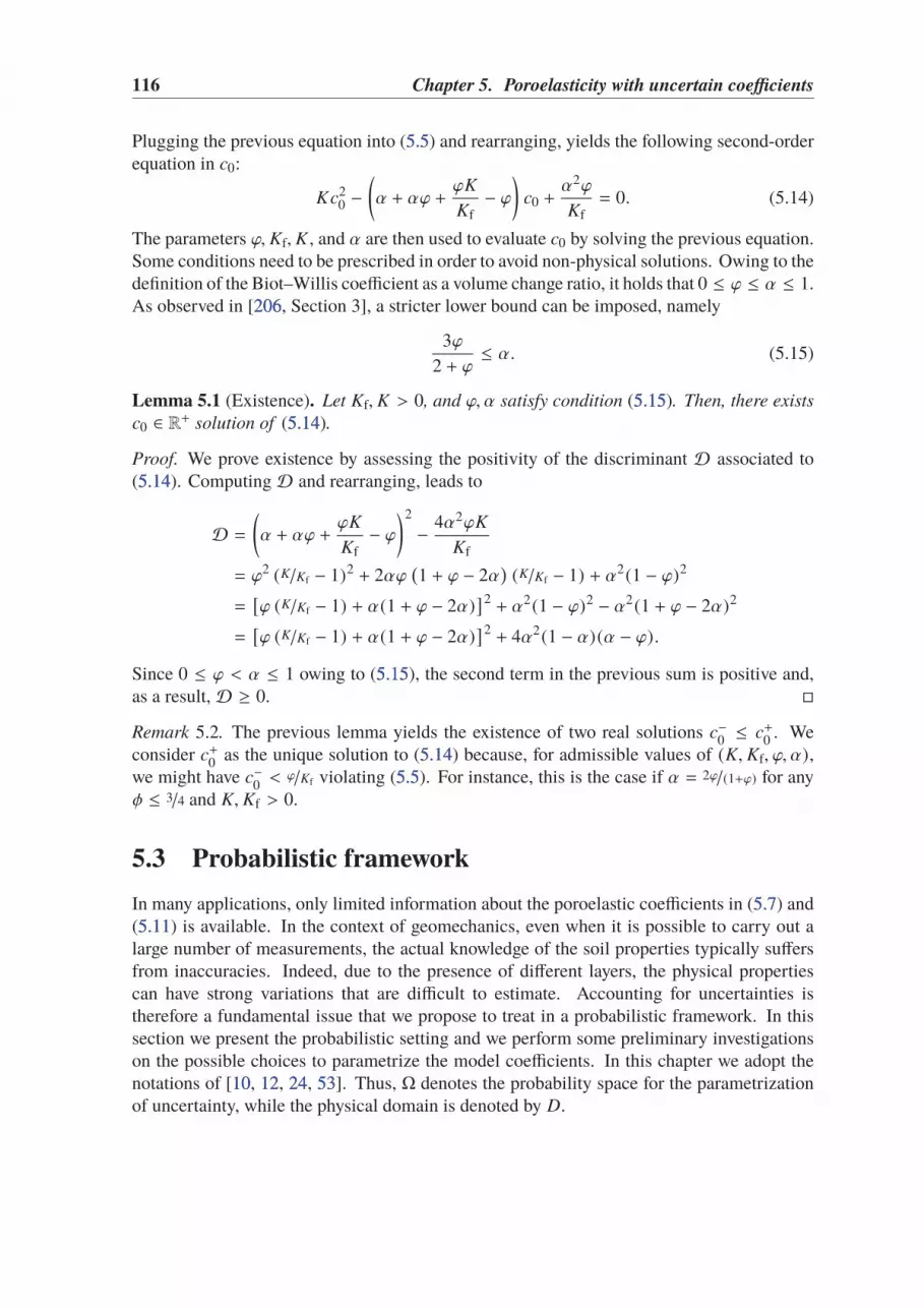
116 Chapter 5. Poroelasticity with uncertain coefficients
Plugging the previous equation into (5.55.5) and rearranging, yields the following second-orderequation in c0:
Kc20 −
(
α + αϕ +ϕK
Kf− ϕ
)
c0 +α2ϕ
Kf= 0. (5.14)
The parameters ϕ, Kf, K , and α are then used to evaluate c0 by solving the previous equation.Some conditions need to be prescribed in order to avoid non-physical solutions. Owing to thedefinition of the Biot–Willis coefficient as a volume change ratio, it holds that 0 ≤ ϕ ≤ α ≤ 1.As observed in [206206, Section 3], a stricter lower bound can be imposed, namely
3ϕ
2 + ϕ≤ α. (5.15)
Lemma 5.1 (Existence). Let Kf, K > 0, and ϕ, α satisfy condition (5.155.15). Then, there exists
c0 ∈ R+ solution of (5.145.14).
Proof. We prove existence by assessing the positivity of the discriminant D associated to(5.145.14). Computing D and rearranging, leads to
D =(
α + αϕ +ϕK
Kf− ϕ
)2
− 4α2ϕK
Kf
= ϕ2 (K/Kf − 1)2+ 2αϕ
(
1 + ϕ − 2α)
(K/Kf − 1) + α2(1 − ϕ)2
=
[
ϕ (K/Kf − 1) + α(1 + ϕ − 2α)]2+ α2(1 − ϕ)2 − α2(1 + ϕ − 2α)2
=
[
ϕ (K/Kf − 1) + α(1 + ϕ − 2α)]2+ 4α2(1 − α)(α − ϕ).
Since 0 ≤ ϕ < α ≤ 1 owing to (5.155.15), the second term in the previous sum is positive and,as a result, D ≥ 0.
Remark 5.2. The previous lemma yields the existence of two real solutions c−0 ≤ c+0 . Weconsider c+0 as the unique solution to (5.145.14) because, for admissible values of (K, Kf, ϕ, α),we might have c−0 < ϕ/Kf violating (5.55.5). For instance, this is the case if α = 2ϕ/(1+ϕ) for anyφ ≤ 3/4 and K, Kf > 0.
5.3 Probabilistic framework
In many applications, only limited information about the poroelastic coefficients in (5.75.7) and(5.115.11) is available. In the context of geomechanics, even when it is possible to carry out alarge number of measurements, the actual knowledge of the soil properties typically suffersfrom inaccuracies. Indeed, due to the presence of different layers, the physical propertiescan have strong variations that are difficult to estimate. Accounting for uncertainties istherefore a fundamental issue that we propose to treat in a probabilistic framework. In thissection we present the probabilistic setting and we perform some preliminary investigationson the possible choices to parametrize the model coefficients. In this chapter we adopt thenotations of [1010, 1212, 2424, 5353]. Thus, Ω denotes the probability space for the parametrizationof uncertainty, while the physical domain is denoted by D.

5.3. Probabilistic framework 117
5.3.1 Notations and basic results
Let n ∈ N and X ⊂ Rn a measurable set. Spaces of functions, vector fields, and tensor fieldsdefined over X are respectively denoted by italic capital, boldface Roman capital, and specialRoman capital letters. Thus, for example, L2(X ), L2(X ), L2(X ) denote the spaces of squareintegrable functions, vector fields, and tensor fields over X respectively. We introduce anabstract probability space (Θ,B,P), where Θ is the set of possible outcomes, B a σ-algebraof events, and P : B → [0, 1] a probability measure. For any random variable h : Θ → Rdefined on the abstract probability space, the expectation of h is
E(h) ≔
∫
Θ
h(θ)dP (θ).
We assume hereafter that all random quantities are second-order ones, namely they belong to
L2P (Θ) ≔
h : Θ→ R : E(h2) < +∞
.
We further introduce a parametrization of the random input data using a random vectorξ = (ξ1, . . . , ξN ) : Θ → Ω ≔ [0, 1]N such that, for all i ∈ 1, . . . , N , ξi ∈ L2
P (Θ) andhas zero mean. For convenience, the random variables ξi are assumed independent, so thatthe probability law Pξ of ξ factorizes. We denote by Bξ the Borel σ-algebra on Ω and by(Ω,Bξ,Pξ ) the image probability space. If, furthermore, each random variable ξi possessesthe density function ρi : [0, 1] → [0,+∞), we may define the space of second-order randomvariables on (Ω,Bξ,Pξ ) as the weighted Lebesgue space L2
ρ(Ω), where the weight function
ρ(ξ ) ≔
n∏
i=1
ρi (ξi)
is the joint density function of ξ . The expectation operator on the image space is denotedusing brackets and is related to the expectation on (Θ,B,P) through the identity
〈h〉 ≔∫
Ω
h(ω)ρ(ω)dω =
∫
Θ
h(ξ (θ))dP (θ) = E(h ξ ).
The variance operator of h ∈ (Ω,Bξ,Pξ ) is then defined by
Var(h) ≔⟨
(h − 〈h〉)2⟩
.
Let D ⊂ Rd , d ∈ 2, 3, denote the spatial domain occupied by the porous medium. For agiven vector space V (D) of real-valued functions on D, equipped with the norm ‖ · ‖V (D), wealso define the Bochner space of second-order random fields by
L2ρ(Ω,V (D)) ≔
v : D ×Ω→ R : ‖v‖L2ρ (Ω,V (D)) ≔
⟨
‖v‖2V (D)
⟩12 < ∞
.

118 Chapter 5. Poroelasticity with uncertain coefficients
0 5 10 15
0
2
4
6
8
10
12
14
16
18
0 5 10 15 20 25 30
K
0.05
0.1
0.15
0.2
0.25
0.3
0.35
0.4
0.45
0.5
Figure 5.1: Left: Scatter plot of 5000 realizations (µ, λ) for K ∼ U ([1, 20]) GPa and ν ∼ U ([0.1, 0.4]). Right:Scatter plot of 5000 realizations (K, ν) for µ ∼ U ([1, 10]) GPa and λ ∼ U ([2, 20]) GPa.
5.3.2 Uncertain poroelastic coefficients
In order to account for the uncertainty of the poroelastic material we model the Lamé’sconstants, the Biot–Willis coefficient, and the hydraulic mobility as spatially varying ran-dom fields depending on the finite-dimensional noise ξ . We represent the random fields(µ, λ, α, κ) : (x, ξ ) ∈ D×Ω→ R4, as affine combinations of the parameters (ξ1, . . . , ξN ) ∈ Ω:
µ(x, ξ ) ≔ µ0(x) +
N∑
i=1
µi (x)ξi, λ(x, ξ ) ≔ λ0(x) +
N∑
i=1
λi (x)ξi,
α(x, ξ ) ≔ α0(x) +
N∑
i=1
αi (x)ξi, κ(x, ξ ) ≔ κ0(x) +
N∑
i=1
κi (x)ξi .
(5.16a)
One well-established approach yielding such functional dependence on the random parametriza-tion is the truncated Karhunen–Loéve expansion [142142, 180180]. According to the results pre-sented in Section 5.2.35.2.3, the constrained specific storage coefficient c0 can be expressed interms of the elastic moduli λ, µ and the coupling Biot coefficient α (see also [6060, 114114] fortheoretical and empirical investigations on the storage coefficient). Therefore, we let
c0(x, ξ ) ≔ c0(µ(x, ξ ), λ(x, ξ ), α(x, ξ )). (5.16b)
In practice, the choice of the elastic parameters describing the mechanical properties ofthe medium is mostly one of convenience. For instance, one might be interested in the Youngmodulus E (e.g. in [128128]), or the bulk modulus K , and the Poisson ratio ν (e.g. in [6060, 173173])instead of µ and λ. For the sake of simplicity, here we choose the Lamé’s coefficients asprimary variables to avoid dealing with nonlinear parametrizations of the model coefficientinducing a warping of the (µ, λ) admissible set as depicted in Figure 5.15.1. However, usingthe truncated Karhunen–Loéve or Polynomial Chaos expansions, it is possible to obtain aparametrization of the model parameter in the affine combination form (5.16a5.16a) even if the

5.3. Probabilistic framework 119
0 5 10 15 20 25 300
0.01
0.02
0.03
0.04
0.05
0.06his
togra
m a
nd p
robabili
ty d
ensity function
0.05 0.1 0.15 0.2 0.25 0.3 0.35 0.4 0.45 0.50
1
2
3
4
5
6
his
tog
ram
an
d p
rob
ab
ility
de
nsity f
un
ctio
n
Figure 5.2: Distribution of the bulk modulus K (left) and the Poisson ration ν (right) corresponding to 106
realizations for µ ∼ U ([1, 10])GPa and λ ∼ U ([2, 20])GPa.
distributions of other elastic moduli are given as entry data. In order to assess the effect ofthe perturbation of the Lamé’s coefficients (µ, λ) as in (5.16a5.16a) on the couple (K, ν), one canuse the relations
K =2
dµ + λ and ν =
λ
2(µ + λ).
We notice that taking (µ, λ) as uniformly distributed primary mechanical variables, neces-sarily yields non-uniform distribution of (K, ν) as illustrated in Figure 5.25.2.
In what follows, we investigate the effect of the parametrization (5.16b5.16b) of c0 on itsprobability distribution. We consider the poromechanical coefficients illustrated in Table 5.15.1.They are inspired from [173173, Table 1], [206206, Section 3], and [6161, Table 4.1], and correspondsto two different layers of an ideal sandstone soil. Since in geophysical applications the fluidbulk modulus and the porosity are usually measurable with sufficient precision, we assumethat Kf and ϕ are deterministic quantities, whereas λ, µ, and α are random variables withuniform distribution, whose ranges are reported in Table 5.15.1. As a particular case of (5.16a5.16a),
Water filled sandstone Water filled deep sandKf 2.2 GPa 2.2 GPaϕ 10% 30%µ U ([1, 10]) GPa U ([5, 80]) KPaλ U ([2, 20]) GPa U ([12, 150]) KPaα U ([3ϕ(2 + ϕ)−1, 1]) U ([3ϕ(2 + ϕ)−1, 1])
Table 5.1: Poromechanical properties
we consider homogeneous random Lamé’s and Biot–Willis coefficients defined such that
µ(ξ ) = µmin + ξ1(µmax − µmin),
λ(ξ ) = λmin + ξ2(λmax − λmin),
α(ξ ) =3ϕ
2 + ϕ+ ξ3
2(1 − ϕ)
2 + ϕ,
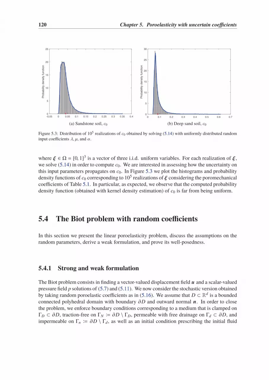
120 Chapter 5. Poroelasticity with uncertain coefficients
-0.05 0 0.05 0.1 0.15 0.2 0.25 0.3 0.35 0.40
5
10
15
20
25
Pro
babili
ty d
ensity function
(a) Sandstone soil, c0
0 0.1 0.2 0.3 0.4 0.5 0.6 0.70
5
10
15
20
25
30
Pro
babili
ty d
ensity f
unction
(b) Deep sand soil, c0
Figure 5.3: Distribution of 105 realizations of c0 obtained by solving (5.145.14) with uniformly distributed randominput coefficients λ, µ, and α.
where ξ ∈ Ω = [0, 1]3 is a vector of three i.i.d. uniform variables. For each realization of ξ ,we solve (5.145.14) in order to compute c0. We are interested in assessing how the uncertainty onthis input parameters propagates on c0. In Figure 5.35.3 we plot the histograms and probabilitydensity functions of c0 corresponding to 105 realizations of ξ considering the poromechanicalcoefficients of Table 5.15.1. In particular, as expected, we observe that the computed probabilitydensity function (obtained with kernel density estimation) of c0 is far from being uniform.
5.4 The Biot problem with random coefficients
In this section we present the linear poroelasticity problem, discuss the assumptions on therandom parameters, derive a weak formulation, and prove its well-posedness.
5.4.1 Strong and weak formulation
The Biot problem consists in finding a vector-valued displacement field u and a scalar-valuedpressure field p solutions of (5.75.7) and (5.115.11). We now consider the stochastic version obtainedby taking random poroelastic coefficients as in (5.165.16). We assume that D ⊂ Rd is a boundedconnected polyhedral domain with boundary ∂D and outward normal n. In order to closethe problem, we enforce boundary conditions corresponding to a medium that is clamped onΓD ⊂ ∂D, traction-free on ΓN ≔ ∂D \ ΓD, permeable with free drainage on Γd ⊂ ∂D, andimpermeable on Γn ≔ ∂D \ Γd , as well as an initial condition prescribing the initial fluid

5.4. The Biot problem with random coefficients 121
content φ0. For a given finite time tF > 0, the resulting problem is given by
−∇·σ (x, ξ, t) + ∇(α(x, ξ )p(x, ξ, t)) = f (x, t), (x, ξ, t) ∈ D ×Ω × (0, tF], (5.17a)
dtφ(x, ξ, t) − ∇·(κ (x, ξ )∇p(x, ξ, t)) = g(x, t), (x, ξ, t) ∈ D ×Ω × (0, tF], (5.17b)
u (x, ξ, t) = 0, (x, ξ, t) ∈ ΓD ×Ω × (0, tF], (5.17c)
σ (x, ξ, t)n + α(x, ξ )p(x, ξ, t))n, = 0 (x, ξ, t) ∈ ΓN ×Ω × (0, tF], (5.17d)
p(x, ξ, t) = 0, (x, ξ, t) ∈ Γd ×Ω × (0, tF], (5.17e)
κ (x, ξ )∇p(x, ξ, t) · n = 0, (x, ξ, t) ∈ Γn ×Ω × (0, tF], (5.17f)
φ(x, ξ, 0) = φ0(x), (x, ξ ) ∈ D ×Ω, (5.17g)
where the stress tensor in (5.17a5.17a) and (5.17d5.17d), and the fluid content in (5.17b5.17b) and (5.17g5.17g),are defined, for all (x, ξ, t) ∈ D ×Ω × (0, tF], such that
σ (x, ξ, t) = 2µ(x, ξ )∇su (x, ξ, t) + λ(x, ξ )(∇·u (x, ξ, t))I d, (5.17h)
φ(x, ξ, t) = c0(x, ξ )p(x, ξ, t) + α(x, ξ )∇·u (x, ξ, t). (5.17i)
If ΓN = Γd = ∅ and c0 = 0, owing to (5.17b5.17b) and the homogeneous Neumann condi-tion (5.17f5.17f), we need the following compatibility conditions on g and φ0 and zero-averageconstraint on p:
∫
D
φ0(·) = 0,
∫
D
g(·, t) = 0, and
∫
D
p(·, ·, t) = 0 ∀t ∈ (0, tF ). (5.17j)
For the sake of simplicity, we exclude the case of ΓD with zero (d−1)-dimensional Hausdorffmeasure. Indeed, this situation simply requires an additional compatibility condition on f
and the prescription of the rigid-body motions of the medium. We remark that other typesof boundary conditions, such as inhomogeneous ones, can also be considered up to minormodifications.
Before giving the variational formulation of problem (5.175.17), we introduce some notations.Let n ∈ N and X ⊂ Rn measurable set. For any m ∈ N, we denote by Hm(X ) the usualSobolev space of functions that have weak partial derivatives of order up to m in L2(X ),with the convention that H0(X ) ≔ L2(X ), while Cm(X ) and C∞
c (X ) denote, respectively,the usual spaces of m-times continuously differentiable functions and infinitely continuouslydifferentiable functions with compact support on X . Since the Biot problem is unsteady, wealso need to introduce, for a vector space V with scalar product (·, ·)V , the Bochner spaceL2((0, tF); V ) spanned by square integrable V -valued functions of the time interval (0, tF).Similarly, the Hilbert space H1(V ) ≔ H1((0, tF); V ) is spanned by V -valued functions ofthe time interval having first-order weak derivative, and the norm ‖·‖H1(V ) is induced by thescalar product
(φ, ψ)H1(V ) =
∫ tF
0(φ(t), ψ(t))V + (dtφ(t), dtψ(t))V dt ∀φ, ψ ∈ H1(V ).
At each time t ∈ (0, tF], the natural functional spaces for the random displacement fieldu (t) : D × Ω → Rd and pressure field p(t) : D × Ω → R taking into account the boundary

122 Chapter 5. Poroelasticity with uncertain coefficients
conditions (5.17c5.17c)–(5.17f5.17f) are, respectively,
U ≔ L2ρ(Ω,H1
0,ΓD(D)),
P ≔
L2ρ(Ω, H1(D) ∩ R(D)⊥) if Γd = ΓN = ∅ and c0 = 0,
L2ρ(Ω, H1
0,Γd(D)) otherwise,
with H10,ΓD
(D) ≔v ∈ H1(D) : v |ΓD = 0
, H1
0,Γd(D) ≔
q ∈ H1(D) : q|Γd = 0
, and
R(D)⊥ ≔
q ∈ L2(D) :
∫
D
q = 0
.
We consider the following weak formulation of problem (5.175.17): For a loading term f ∈L2((0, tF),L2(D)), a fluid source g ∈ L2((0, tF), L2(D)), and an initial datum φ0 ∈ L2(D)
that verify (5.17j5.17j), find u ∈ L2((0, tF),U ) and p ∈ L2((0, tF), P) such that, for all v ∈ U , allq ∈ P, and all ψ ∈ C∞
c ((0, tF))
∫ tF
0a(u (t), v ) ψ(t)dt +
∫ tF
0b(v, p(t)) ψ(t)dt =
∫ tF
0
⟨
( f (t), v )D
⟩
ψ(t)dt,
(5.18a)∫ tF
0
[
b(u (t), q) − c(p(t), q)]
dtψ(t)dt +
∫ tF
0d(p(t), q) ψ(t)dt =
∫ tF
0〈(g(t), q)D〉ψ(t)dt,
(5.18b)
c(p(0), q) − b(u (0), q) = 〈(φ0, q)D〉 , (5.18c)
where (·, ·)D denotes the usual inner product in L2(D) and the bilinear forms a : U ×U → R,b : U × P → R, and c : P × P → R are defined such that, for all v, w ∈ U and all q, r ∈ P,
a(v, w ) ≔
∫
Ω
∫
D
(
2µ(x, ξ )∇sv (x, ξ ) : ∇sw (x, ξ ) + λ(x, ξ )∇·v (x, ξ )∇·w (x, ξ ))
ρ(ξ ) dxdξ,
b(v, q) ≔ −∫
Ω
∫
D
α(x, ξ )∇·v (x, ξ )q(x, ξ )ρ(ξ ) dxdξ,
c(q, r) ≔
∫
Ω
∫
D
c0(x, ξ )q(x, ξ )r (x, ξ )ρ(ξ ) dxdξ,
d(q, r) ≔
∫
Ω
∫
D
κ(x, ξ )∇r (x, ξ ) · ∇q(x, ξ )ρ(ξ ) dxdξ .
Above, we have introduced the Frobenius product such that, for all τ, η ∈ Rd×d , τ : η ≔∑
1≤i, j≤d τi jηi j with corresponding norm such that, for all τ ∈ Rd×d , |τ |d×d ≔ (τ : τ)1/2.
5.4.2 Well-posedness
The aim of this section is to infer a stability estimate on the displacement and pressure (u, p) ∈L2((0, tF),U ) × L2((0, tF), P) solving (5.185.18), yielding, in particular, the well-posedness ofthe weak problem. The existence and uniqueness of a solution to the deterministic Biot

5.4. The Biot problem with random coefficients 123
problem has been studied in [181181, 205205]. The results therein establish the existence. foralmost every (a.e.) ξ ∈ Ω, of a solution (u (ξ ), p(ξ )) to (5.175.17). Thus, proving that themapping ξ → (u (ξ ), p(ξ )) is measurable and bounded in L2
ρ(Ω) gives the existence of asolution to (5.185.18).
We assume some additional conditions on the input random fields defined in (5.165.16) thatwill be needed in the proofs. First, we recall that, for all x ∈ D and all ξ ∈ Ω the couplingcoefficient α(x, ξ ) ∈ (0, 1] satisfies the lower bound (5.155.15). We assume that the referenceporosity of the medium is strictly positive (otherwise the Biot problem would reduce to adecoupled one), so that we have 0 < α ≔
3ϕ2+ϕ < α(x, ξ ). We also assume that the Lamé’s
coefficients satisfies the following:Assumption 5.3 (Elastic moduli). The shear modulus µ ∈ L∞(D ×Ω) is uniformly boundedfrom above and away from zero, i.e. there exist positive constants µ and µ such that
0 < µ ≤ µ(x, ξ ) ≤ µ < ∞, a.e. in D ×Ω. (5.19)
The dilatation modulus λ ∈ L∞(D×Ω) is uniformly bounded, i.e. there exist λ > 0 such that
0 < λ(x, ξ ) ≤ λ < ∞, a.e. in D ×Ω. (5.20)
The next result establishes the coercivity and the inf-sup condition respectively of thebilinear form a and b appearing in (5.18a5.18a).Lemma 5.4 (Coercivity and inf-sup). Under Assumption 5.35.3, the following bounds hold
a(v, v ) ≥ 2µ C−1K ‖v ‖2
U, ∀v ∈ U, (5.21)
sup0,v∈U
b(v, q)
‖v ‖U≥ α Cis‖q‖L2
ρ (Ω,L2(D)), ∀q ∈ L2ρ(Ω, L2(D)), (5.22)
where CK > 0 denotes the constant in Korn’s first inequality, and Cis > 0 the inf-sup constant.
In the case ΓD = ∂D, (5.225.22) holds for all q ∈ L2ρ(Ω, L2(D) ∩ R(D)⊥).
Proof. The first bound directly follows from Assumption 5.35.3. Indeed, since |ΓD |d−1 > 0, wecan apply Korn’s first inequality, yielding
2µ‖∇v ‖2L2ρ (Ω,L2(D))
≤ 2µCK
⟨
‖∇sv ‖2L2(D)
⟩
≤ CKa(v, v ), ∀v ∈ U .
To obtain (5.225.22), we use [2424, Lemma 7.2] establishing the existence, for any q ∈ L2ρ(Ω, L2(D))
(or q ∈ L2ρ(Ω, L2(D) ∩ R(D)⊥) in the case Γd = ∂D), of vq ∈ U such that ∇·vq = q and
Cis‖vq‖U ≤ ‖q‖L2ρ (Ω,L2(D)), with Cis > 0 depending on D. Thus, we conclude
sup0,v∈U
b(v, q)
‖v ‖U≥−b(vq, q)
‖vq‖U≥α‖q‖2
L2ρ (Ω,L2(D))
‖vq‖U≥ α Cis‖q‖L2
ρ (Ω,L2(D)) .

124 Chapter 5. Poroelasticity with uncertain coefficients
In order to prove the stability estimate of Proposition 5.55.5 below, we infer from (5.195.19) and(5.205.20) a lower bound of the specific storage coefficient c0. We rewrite (5.135.13), derived fromthe definition of α in (5.45.4) and the Gassmann equation (5.125.12), in the form
(1 − α)(Km − K )
α= K − α
c0.
Since the left-hand side of the previous relation is always non-negative (according to [6161,Chapter 4] we have Kd ≤ K ≤ Km), we infer that α/c0 ≤ K and, as a result,
c−10 (x, ξ ) ≤ K (x, ξ )
α(x, ξ )=
2µ(x, ξ ) + dλ(x, ξ )
dα(x, ξ )≤ 2µ + dλ
dαa.e. in D ×Ω. (5.23)
Proposition 5.5 (A priori estimate). Let (u, p) ∈ L2((0, tF),U × P) solve (5.185.18). Under
Assumption 5.35.3, it holds
∫ tF
0
[
a(u (t), u (t)) + c(p(t), p(t))]
dt ≤∫ tF
0
CK
2µ‖ f ‖2
L2(D)+
2µ + dλ
dα‖G‖2
L2(D)
dt,
(5.24)with G : (0, tF) → L2(D) defined by
G(t) ≔
∫ t
0g(s)ds + φ0. (5.25)
Proof. From (5.18a5.18a) we infer that a(u (t), v ) + b(v, p(t)) =(
f (t), 〈v〉)D, for a.e. t ∈ (0, tF)
and all v ∈ U . Setting v (x, ξ ) = u (x, ξ, t) and integrating the previous relation on (0, tF),yields
∫ tF
0a(u (t), u (t))dt +
∫ tF
0b(u (t), p(t))dt =
∫ tF
0
(
f (t), 〈u (t)〉)D dt. (5.26)
Adapting the argument of Remark 4.24.2 we ensure that b(u (t), q)− c(p(t), q) ∈ H1((0, tF)) forall q ∈ P. Thus, we can integrate by parts (5.18b5.18b) and obtain
dt
[
c(p(s), q) − b(u (s), q)]
+ d(p(s), q) =(
g(s), 〈q〉)D , for a.e. s ∈ (0, tF).
Letting t ∈ (0, tF), integrating the previous identity on (0, t), and then taking q(x, ξ ) =
p(x, ξ, t), leads to
c(p(t), p(t)) − b(u (t), p(t)) +
∫ t
0d(p(s), p(t))ds =
∫ t
0
(
g(s), 〈p(t)〉)D ds +(
φ0, 〈p(t)〉)D .
We define z(t) =∫ t
0p(s)ds and observe that dt z(t) = p(t) and z(0) = 0. Using the linearity
of d and the formula dt z2(t) = 2z(t)dt z(t) to rewrite the third term in the left hand side of
the previous relation, and recalling (5.255.25) we get
c(p(t), p(t)) − b(u (t), p(t)) +1
2dt [d(z(t), z(t))] =
(
G(t), 〈p(t)〉)D ds.

5.4. The Biot problem with random coefficients 125
Then, integrating on (0, tF) and summing the resulting identity to (5.265.26), gives
∫ tF
0a(u (t), u (t))dt +
∫ tF
0c(p(t), p(t))dt +
1
2d(z(tF), z(tF)) =
∫ tF
0
(
f (t), 〈u (t)〉)D dt +
∫ tF
0
(
G(t), 〈p(t)〉)D dt . (5.27)
To establish the result, we now bound the right-hand side of the previous relation. First, weobserve that, owing to the Jensen inequality, for all v ∈ U it holds
‖〈v〉‖2L2(D)
=
∫
D
(∫
Ω
v (x, ξ )ρ(ξ )dξ
)2
dx ≤∫
Ω
∫
D
v (x, ξ )2ρ(ξ ) dxdξ ≤ ‖v ‖2U .
Using the previous relation and the Cauchy–Schwarz and Young inequalities followed by(5.215.21), it is inferred that
∫ tF
0
(
f (t), 〈u (t)〉)D dt ≤∫ tF
0(2µC−1
K )−1/2‖ f ‖L2(D) (2µC−1
K )1/2‖u ‖Udt
≤ CK
4µ
∫ tF
0‖ f ‖2
L2(D)dt +
1
2
∫ tF
0a(u (t), u (t))dt .
Proceeding similarly for the second term in the right-hand side of (5.275.27) and recalling thelower bound (5.235.23), one has
∫ tF
0
(
G(t), 〈p(t)〉)D dt ≤∫ tF
0‖c−1/2
0 G‖L2ρ (Ω,L2(D)) ‖c
1/20 p‖L2
ρ (Ω,L2(D))dt
≤ 2µ + dλ
2dα
∫ tF
0‖G‖2
L2(D)dt +
1
2
∫ tF
0c(p(t), p(t))dt.
Plugging the previous two estimates in (5.275.27), multiplying by a factor 2, and using thenon-negativity of κ to infer d(z(tF), z(tF)) ≥ 0, yields the conclusion.
Some remarks are in order.
Remark 5.6 (Inf-sup conditon). We observe that it is possible to derive the previous a prioriestimate without (5.235.23). Indeed the inf-sup condition (5.225.22) together with (5.18a5.18a) allows tobound the second term in the right-hand side of (5.275.27) using the following: for a.e. t ∈ (0, tF),
‖p(t)‖L2ρ (Ω,L2(D)) ≤ (αCis)
−1 sup0,v∈U
b(v, p(t))
‖v ‖U= (αCis)
−1 sup0,v∈U
( f (t), 〈v〉)D − a(u (t), v )
‖v ‖U
≤ 1
αCis‖ f (t)‖L2(D) +
(2µ + dλ)1/2
d1/2αCisa(u (t), u (t))
1/2.
The resulting stability estimate would have, compared to (5.245.24), an additional dependence onαCis.
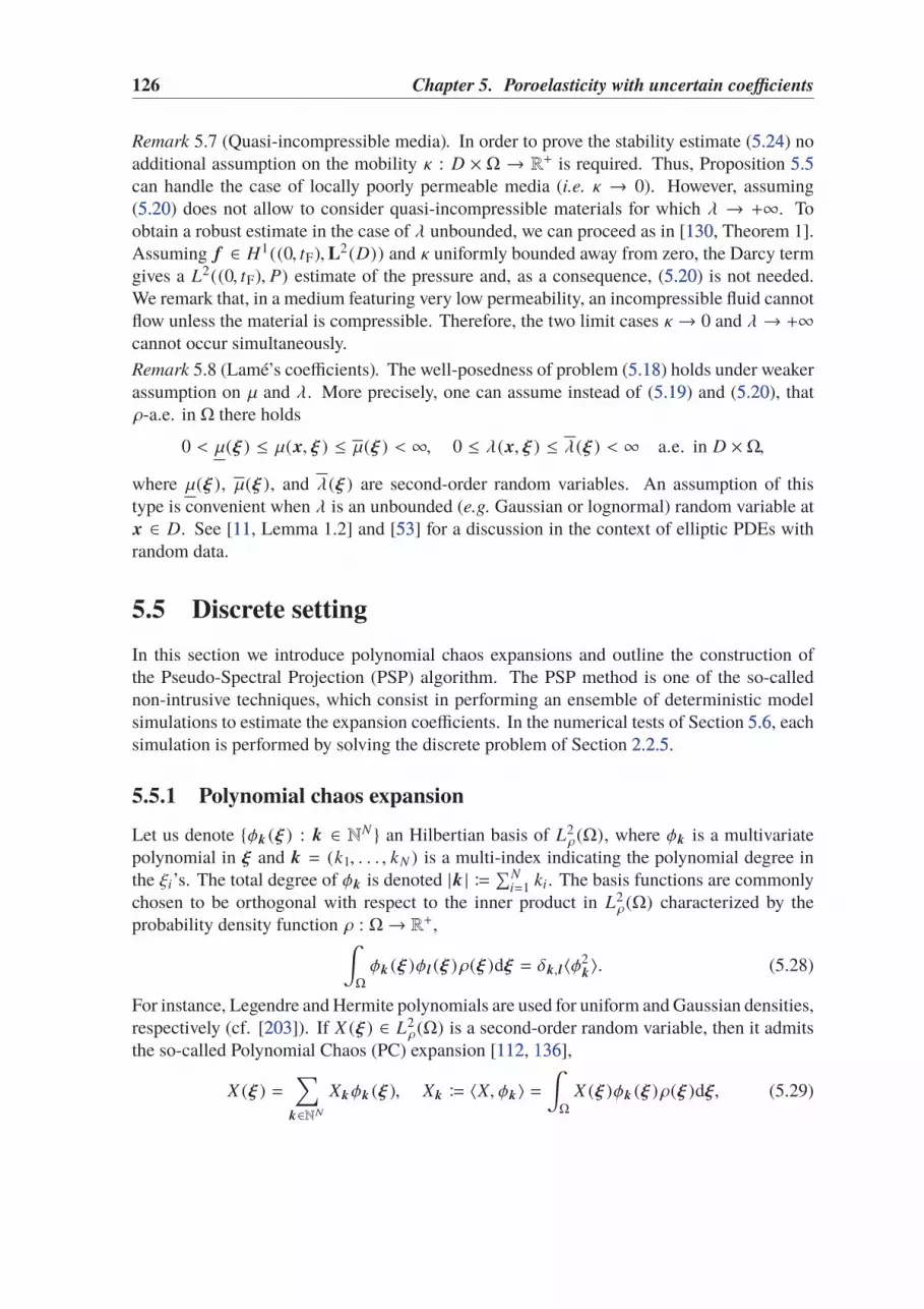
126 Chapter 5. Poroelasticity with uncertain coefficients
Remark 5.7 (Quasi-incompressible media). In order to prove the stability estimate (5.245.24) noadditional assumption on the mobility κ : D × Ω → R+ is required. Thus, Proposition 5.55.5can handle the case of locally poorly permeable media (i.e. κ → 0). However, assuming(5.205.20) does not allow to consider quasi-incompressible materials for which λ → +∞. Toobtain a robust estimate in the case of λ unbounded, we can proceed as in [130130, Theorem 1].Assuming f ∈ H1((0, tF),L2(D)) and κ uniformly bounded away from zero, the Darcy termgives a L2((0, tF), P) estimate of the pressure and, as a consequence, (5.205.20) is not needed.We remark that, in a medium featuring very low permeability, an incompressible fluid cannotflow unless the material is compressible. Therefore, the two limit cases κ → 0 and λ → +∞cannot occur simultaneously.
Remark 5.8 (Lamé’s coefficients). The well-posedness of problem (5.185.18) holds under weakerassumption on µ and λ. More precisely, one can assume instead of (5.195.19) and (5.205.20), thatρ-a.e. in Ω there holds
0 < µ(ξ ) ≤ µ(x, ξ ) ≤ µ(ξ ) < ∞, 0 ≤ λ(x, ξ ) ≤ λ(ξ ) < ∞ a.e. in D ×Ω,
where µ(ξ ), µ(ξ ), and λ(ξ ) are second-order random variables. An assumption of thistype is convenient when λ is an unbounded (e.g. Gaussian or lognormal) random variable atx ∈ D. See [1111, Lemma 1.2] and [5353] for a discussion in the context of elliptic PDEs withrandom data.
5.5 Discrete setting
In this section we introduce polynomial chaos expansions and outline the construction ofthe Pseudo-Spectral Projection (PSP) algorithm. The PSP method is one of the so-callednon-intrusive techniques, which consist in performing an ensemble of deterministic modelsimulations to estimate the expansion coefficients. In the numerical tests of Section 5.65.6, eachsimulation is performed by solving the discrete problem of Section 2.2.52.2.5.
5.5.1 Polynomial chaos expansion
Let us denote φk (ξ ) : k ∈ NN an Hilbertian basis of L2ρ(Ω), where φk is a multivariate
polynomial in ξ and k = (k1, . . . , kN ) is a multi-index indicating the polynomial degree inthe ξi’s. The total degree of φk is denoted |k | ≔ ∑N
i=1 ki. The basis functions are commonlychosen to be orthogonal with respect to the inner product in L2
ρ(Ω) characterized by theprobability density function ρ : Ω→ R+,
∫
Ω
φk (ξ )φl (ξ )ρ(ξ )dξ = δk,l〈φ2k〉. (5.28)
For instance, Legendre and Hermite polynomials are used for uniform and Gaussian densities,respectively (cf. [203203]). If X (ξ ) ∈ L2
ρ(Ω) is a second-order random variable, then it admitsthe so-called Polynomial Chaos (PC) expansion [112112, 136136],
X (ξ ) =∑
k∈NN
Xkφk (ξ ), Xk ≔ 〈X, φk〉 =∫
Ω
X (ξ )φk (ξ )ρ(ξ )dξ, (5.29)

5.5. Discrete setting 127
where the deterministic coefficients of the series Xk : k ∈ NN , named the spectral modes,are defined as the projection of X (ξ ) onto the basis functions. The PC approximation XK (ξ )
of X (ξ ) is obtained by truncating the expansion above to a finite series,
XK (ξ ) ≔∑
k∈KXkφk (ξ ), (5.30)
whereK ⊂ NN is the set of multi-indices related to the expansion. As a result, the expectationand variance operators applied to PC approximations simplify as follows:
〈XK 〉 = X0, (5.31)
Var(XK ) =∑
k∈K \0X2k〈φ
2k〉. (5.32)
The truncation strategy, i.e. the selection of the set K , depends on the method used tocompute the spectral modes and the error eK (ξ ) := X (ξ ) − XK (ξ ) decreases when thePC degree increases. The convergence rate of the PC expansion of X with respect to thePC degree depends on the regularity of X . In particular, an exponential convergence isexpected for analytical variables; more details about the convergence conditions can be foundin [4646, 9898]. Several methods can be implemented to compute the spectral modes of the PCexpansion [125125, 136136, 137137] such as pseudo-spectral projection, least squares regression, andcompressed sensing. These procedures mainly differ in the specific discrete norm used forminimizing the truncation error eK (ξ ). They are non-intrusively implemented by evaluatingX (ξ ) at a finite number of values of ξ (the design of experiments) and therefore requireonly the availability of a deterministic solver. We focus here on the non-intrusive spectralprojection approach [5858, 5959, 171171] designed to avoid internal aliasing (the violation of theorthogonality condition (5.285.28) at the discrete level). The spectral projection method uses aquadrature rule in order to compute the spectral modes Xk by approximating (5.295.29),
Xk = 〈X, φk〉 ≃Np∑
q=1
wq X (ξ (q))φk (ξ (q)), (5.33)
where ξ (q) and wq are the Np integration points and associated weights. The previousequation shows that the main computational burden of the non-intrusive spectral projectiontechnique is to compute Np model evaluations for X (ξ ( j)). In traditional tensor-productquadrature rules, Np scales exponentially with the number of parameters N (the so-called"Curse of Dimensionality") and is intractable for all but very low dimensional problem. Thisissue has motivated the use of sparse quadrature formulas, which significantly reduce thecomputational cost.
5.5.2 Sparse Pseudo-Spectral Projection
In the numerical tests of Section 5.65.6, we rely on the sparse Pseudo-Spectral Projection (PSP)method that is based on the partial tensorization of nested one-dimensional quadrature rules

128 Chapter 5. Poroelasticity with uncertain coefficients
0 0.2 0.4 0.6 0.8 1
Location of integration Points
3
2
1
0
Level
(a) Uniform points
0 0.2 0.4 0.6 0.8 1
Location of integration Points
3
2
1
0
Level
(b) Clenshaw–Curtis points
Figure 5.4: Examples of 1-D nested sequences including 1, 3, 5, and 9 quadrature points.
via Smolyak’s formula [184184]. Consider Q0,Q1,Q2, . . . a nested sequence of 1-D quadratureformulas having increasing polynomial exactness p0, p1, p2, . . ., that is
∫ 1
0F (ξ)ρ(ξ)dξ = Ql F =
Np (l)∑
q=1
F(
ξ (q,l))
w(q,l)1D
, ∀F ∈ Ppl ([0, 1]),
where Np(l) is the number of points in the formula Ql and Ppl ([0, 1]) denotes the spacespanned by polynomials of total degree pl . We call l the level of the formula Ql . Figure 5.45.4shows 1-D nested sequences over the interval [0, 1] for level 1 ≤ l ≤ 3 associated withuniform and Clenshaw–Curtis points.
Prescribing the multi-index l = (l1, . . . , lN ) ∈ NN , the full tensor-product quadrature ofan integrable function F, can be written as follows:
QFTl F ≔
(
Ql1 ⊗ · · · ⊗ QlN
)
F =
Np (l1)∑
q1=1
· · ·Np (lN )∑
qd=1
F(
ξ(q1,l1)
1 , . . . , ξ(qN ,lN )
N
)
w(q1,l1)
1D· · ·w(qN ,lN )
1D.
(5.34)The previous quadrature rule can be used in (5.335.33) to compute the spectral modes Xk ,using F = Xφk , for all k ∈ K . The complexity of QFT
lfor such nested sequences is
Np(l) =∏N
i=1 Np(li), and so it increases exponentially with N . Sparse grids mitigate thiscomplexity by first introducing the 1-D difference formulas between two successive levels,∆
Q
l= Ql −Ql−1, ∆Q
0 = Q0, such that (5.345.34) can be reformulated as
QFTl F =
*.,*.,
l1∑
i1=0
∆Q
i1
+/- ⊗ · · · ⊗*.,
lN∑
iN=0
∆Q
iN
+/-+/- F =
l1∑
i1=0
· · ·lN∑
iN=0
(
∆Q
i1⊗ · · · ⊗ ∆Q
iN
)
F =∑
i∈LFTl
∆Q
iF,
where LFTl= i ∈ NN, i j ≤ l j for j = 1, . . . , d is the multi-index set of full tensorizations.
The sparse quadrature rule QL is finally constructed by considering the summation over a
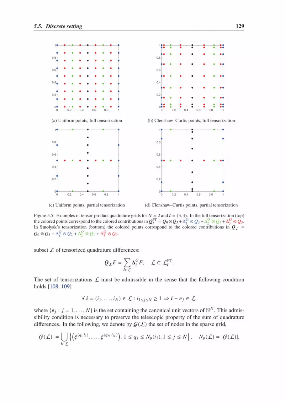
5.5. Discrete setting 129
0 0.2 0.4 0.6 0.8 1
0
0.2
0.4
0.6
0.8
1
(a) Uniform points, full tensorization
0 0.2 0.4 0.6 0.8 1
0
0.2
0.4
0.6
0.8
1
(b) Clenshaw–Curtis points, full tensorization
0 0.2 0.4 0.6 0.8 1
0
0.2
0.4
0.6
0.8
1
(c) Uniform points, partial tensorization
0 0.2 0.4 0.6 0.8 1
0
0.2
0.4
0.6
0.8
1
(d) Clenshaw–Curtis points, partial tensorization
Figure 5.5: Examples of tensor-product quadrature grids for N = 2 and l = (3, 3). In the full tensorization (top)the colored points correspond to the colored contributions in QFT
l= Q0 ⊗Q3+∆
Q
1 ⊗ Q3+∆Q
2 ⊗ Q3+∆Q
3 ⊗ Q3.In Smolyak’s tensorization (bottom) the colored points correspond to the colored contributions in QL =
Q0 ⊗ Q3 + ∆Q
1 ⊗ Q2 + ∆Q
2 ⊗ Q1 + ∆Q
3 ⊗ Q0.
subset L of tensorized quadrature differences:
QLF =∑
i∈L∆
Q
iF, L ⊂ LFT
l .
The set of tensorizations L must be admissible in the sense that the following conditionholds [108108, 109109]
∀ i = (i1, . . . , iN ) ∈ L : i1≤ j≤N ≥ 1 ⇒ i − e j ∈ L,
where e j : j = 1, . . . , N is the set containing the canonical unit vectors of NN . This admis-sibility condition is necessary to preserve the telescopic property of the sum of quadraturedifferences. In the following, we denote by G(L) the set of nodes in the sparse grid,
G(L) ≔⋃
i∈L
(ξ (q1,i1), . . . , ξ (qN ,iN )
)
, 1 ≤ qj ≤ Np(i j ), 1 ≤ j ≤ N, Np(L) = |G(L) |,

130 Chapter 5. Poroelasticity with uncertain coefficients
where | · | is the cardinality of a set. In Figure 5.55.5 we plot the grids corresponding to full andsparse tensor-product quadrature rules in the case of N = 2 and l = (3, 3).
A quadrature rule QL is said to be sufficiently exact with respect to a polynomial multi-index setK when for any couple (k, k′) ∈ K ×K , the basis orthonormality conditions (5.285.28)are recovered using the discrete inner product defined, for all X,Y ∈ L2
ρ(Ω), by
〈X,Y 〉QL ≔ QL (XY ).
In the case of full tensorizations, the largest setK ∗(l) for which internal aliasing errors vanishcan be easily determined from the degrees of polynomial exactness of the 1-D sequence,namely
K ∗(l) =
k ∈ NN : ki ≤pli
2, i = 1, . . . , N
.
An immediate consequence of using the sparse quadrature formula with L ⊂ LFTl
, is thatQL is not sufficiently exact with respect toK ∗(l), as the sparse formula is not able to exactlyintegrate the product of high-order monomials. We observe that the use of sparse quadrature,while reducing the complexity (Np(L) ≪ ∏N
j=1 Np(l j )), yields also a significant reductionof the (not uniquely-defined) largest setK ∗(L) for which the quadrature is sufficiently exact.
The PSP method allows to consider polynomial spaces larger than K ∗(L), for the samesparse grid G(L) and without introducing internal aliasing. Let Πl l≥1 denote the sequenceof 1-D projection operators associated to the sequence Ql l ≥ 1 of 1-D nested quadrature,where
Πl : X (ξ) 7→ Πl X (ξ) ≔
pl/2∑
k=0
Xkφk (ξ) ∈ Ppl2 ([0, 1]), Xk =
Np (l)∑
q=1
X (ξ (q,l))φk (ξ (q,l))w(q,l)1D
.
Note that Πl≥1 is free of internal aliasing, owing to the dependence on l of the projectionspaces, which ensures that the quadrature is sufficiently exact. Consider for l ≥ 1 thedifference of successive 1-D projection operators ∆Π
l>1 = Πl − Πl−1, ∆Π1 = Π1. It ispossible to write the full tensor-product projection corresponding to the quadrature rulegiven by (5.345.34) in terms of a sum of tensorized difference operators by observing that
ΠFTl X ≔
∑
k∈K ∗(l)
QFTl (Xφk )(ξ ) =
(
Πl1 ⊗ · · · ⊗ ΠlN
)
X
=
l1∑
i1=1
· · ·lN∑
iN=1
(
∆Πi1 ⊗ · · · ⊗ ∆ΠiN
)
X =∑
i∈LFTl
(
∆Πi1 ⊗ · · · ⊗ ∆ΠiN
)
X .
The sparse PSP operatorΠL is finally obtained by considering a summation over an admissiblesubset L ⊂ LFT
lof tensorized difference projection operators. This results in
ΠLX =∑
i∈L
(
∆Πi1 ⊗ · · · ⊗ ∆ΠiN
)
X . (5.35)
The key point is that the sparse PSP operator in (5.355.35) involves a telescopic sum of differences

5.6. Test cases 131
PSP Polynomials
Direct Projection Polynomials
Polynomial Exactness
k2
k1
0 5 10 15
0
5
10
15
Figure 5.6: Comparison of polynomials multi-index sets K (L) (below the red line) and K ∗(L) (belowthe blue line) using a quadrature rule QL in d = 2 dimensions. Points are multi-indices (k1, k2) suchF ∈ Pk1 ([0, 1]) × Pk1 ([0, 1]) is exactly integrated by QL .
in the projection onto subspaces of increasing dimensions, where each individual tensorizedquadrature projection is evaluated without internal aliasing. Moreover, ΠL belongs to thespan of φk : k ∈ K (L), with K (L) =
⋃
i∈L K ∗(i). We have K (L) ⊇ K ∗(L) and theprojection space of the sparse PSP is usually significantly larger than that of the direct sparseprojection. Nevertheless, the two methods have the same complexity relying both on the samesparse grid G(L). Note, however, that the global sparse quadrature rule QL is generally notsufficiently accurate with respect to K (L). The inclusion of the sets K (L) and K ∗(L) isillustrated in Figure 5.65.6.
5.6 Test cases
We assess the performance of the PSP method detailed in the previous section on two modelproblems. The first one is an injection test designed to investigate the effect of a fluid sourceon the deformation of the domain, while the second one is meant to evaluate the mechanicaleffect of a traction term on the flux. Our numerical experiments feature a simplified modelwith homogeneous random coefficients, namely the dependence of the spacial variable x in(5.165.16) is dropped. More realistic models, requiring (possibly strongly correlated) spatiallyvarying input coefficients with non-standard distributions will be the object of future works.After presenting the description of the test cases, we numerically investigate the convergenceof the probability error with respect to the level of the sparse grid. Finally, we perform asensitivity analysis in order to rank the contribution of the input parameters on the varianceof the solutions.
Our input uncertainty is parametrized by a vector ξ of dimension N = 4. In particular,we assume that µ, λ, and κ have a log-uniform distribution, while α is uniformly distributed.As proposed in Section 5.3.25.3.2, the specific storage coefficient c0 is evaluated from the otheruncertain input parameters. The advantage of this approach is twofold: (i) it ensures that

132 Chapter 5. Poroelasticity with uncertain coefficients
the set of poroelastic coefficients belong to the physical admissible set, and (ii) it allows toreduce the uncertainty dimension and then the size of the sampling (i.e. , number of sparsegrid points). Even if the experiments presented here are mainly academic model problems,we try to consider realistic sets of parameters and have a particular regard for the underlyingphysical phenomena. The ranges of variation of the uncertain input data are inspired from anideal water filled sand soil with a ϕ = 20% reference porosity. In both tests we set
µ(ξ ) = 102ξ1 KPa,
λ(ξ ) = 2 · 102ξ2 KPa,
α(ξ ) =3ϕ
2 + ϕ+ ξ3
2(1 − ϕ)
2 + ϕ,
κ(ξ ) = 102(ξ4−1) m2KPa−1s−1,
(5.36)
with uniformly distributed (ξ1, . . . , ξ4) ∈ [0, 1]4. This choice yields
〈µ〉 ∼ 21.5 KPa, 〈λ〉 ∼ 43 KPa, 〈α〉 ∼ 0.64, and 〈κ〉 ∼ 0.22m2
KPa s,
cv(µ) ∼ 1.16, cv(λ) ∼ 1.16, cv(α) ∼ 0.33, and cv(κ) ∼ 1.16,(5.37)
where cv(·) ≔ Var(·)1/2
〈·〉 denotes the coefficient of variation operator. In particular we observethat the previous average values have the same magnitude as the coefficients consideredin [102102, Table 2]. Our choice leads to a specific storage coefficient c0 ranging in (10−3, 10−1).
5.6.1 Point injection
The first experiment is inspired by the Barry and Mercer test considered in Section 2.6.22.6.2(see also [1414, 166166]). On the boundary of the unit square domain D = [0, 1]2 we impose thefollowing time-independent homogeneous boundary conditions:
u · τ = 0, nT∇un = 0, p = 0,
where τ denotes the tangent vector on ∂D. The loading term f in (5.17a5.17a) and the initialcondition φ0 in (5.17g5.17g) are both chosen to be zero. The evolution of the displacementand pressure fields solving (5.175.17) is only driven by a stationary fluid source located atx0 = (0.25, 0.25):
g = 10 δ(x − x0),
with δ denoting the Dirac delta function. The following results have been obtained using theHHO–dG coupled method with polynomial degree k = 3 on a Cartesian mesh containing1,024 elements. Using the static condensation procedure detailed in Section 2.52.5, the spacialdiscretization consists of 27,648 unknowns. We are interested in the stationary solution,namely the pressure and displacement fields manifesting after the initial transient phase.Therefore, we only focus on the configuration at the final time tF = 1s obtained after 10 timesteps of the implicit Euler scheme.
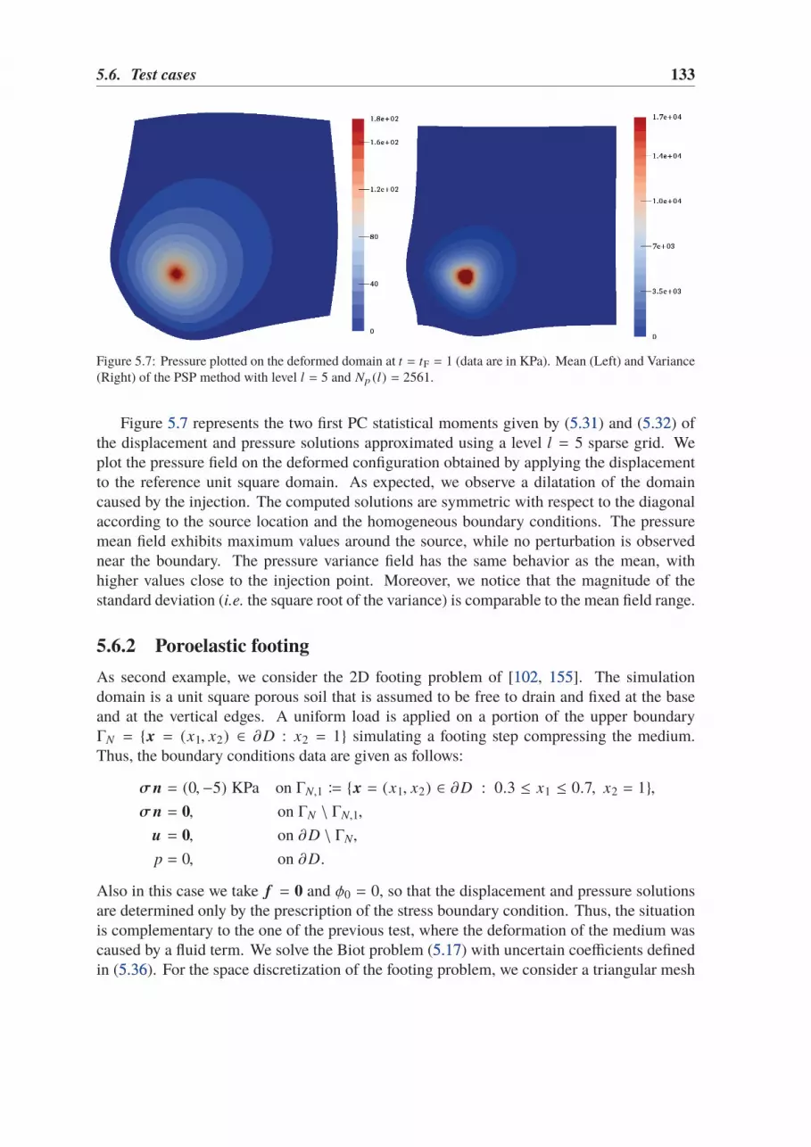
5.6. Test cases 133
Figure 5.7: Pressure plotted on the deformed domain at t = tF = 1 (data are in KPa). Mean (Left) and Variance(Right) of the PSP method with level l = 5 and Np (l) = 2561.
Figure 5.75.7 represents the two first PC statistical moments given by (5.315.31) and (5.325.32) ofthe displacement and pressure solutions approximated using a level l = 5 sparse grid. Weplot the pressure field on the deformed configuration obtained by applying the displacementto the reference unit square domain. As expected, we observe a dilatation of the domaincaused by the injection. The computed solutions are symmetric with respect to the diagonalaccording to the source location and the homogeneous boundary conditions. The pressuremean field exhibits maximum values around the source, while no perturbation is observednear the boundary. The pressure variance field has the same behavior as the mean, withhigher values close to the injection point. Moreover, we notice that the magnitude of thestandard deviation (i.e. the square root of the variance) is comparable to the mean field range.
5.6.2 Poroelastic footing
As second example, we consider the 2D footing problem of [102102, 155155]. The simulationdomain is a unit square porous soil that is assumed to be free to drain and fixed at the baseand at the vertical edges. A uniform load is applied on a portion of the upper boundaryΓN = x = (x1, x2) ∈ ∂D : x2 = 1 simulating a footing step compressing the medium.Thus, the boundary conditions data are given as follows:
σn = (0,−5) KPa on ΓN,1 ≔ x = (x1, x2) ∈ ∂D : 0.3 ≤ x1 ≤ 0.7, x2 = 1,σn = 0, on ΓN \ ΓN,1,
u = 0, on ∂D \ ΓN,
p = 0, on ∂D.
Also in this case we take f = 0 and φ0 = 0, so that the displacement and pressure solutionsare determined only by the prescription of the stress boundary condition. Thus, the situationis complementary to the one of the previous test, where the deformation of the medium wascaused by a fluid term. We solve the Biot problem (5.175.17) with uncertain coefficients definedin (5.365.36). For the space discretization of the footing problem, we consider a triangular mesh

134 Chapter 5. Poroelasticity with uncertain coefficients
Figure 5.8: Pressure plotted on the deformed domain at t = 0.2. Mean (left) and Variance (right) computedusing the PSP method with level l = 5 and Np (l) = 2561.
with 3,584 elements and we use the HHO–dG method with k = 2. For each point of the sparsegrid and each time iteration, the linear system to be solved has dimension 54,720. In this testcase, we are particularly interested in the pressure profile at early times. In fact, owing tothe free drainage boundary condition, after a few time steps the fluid is completely squeezedout of the soil, yielding an equilibrium configuration with no pressure and the displacementbalancing the Neumann condition. We consider the approximated solution at time t = 0.2sobtained after two time steps of the implicit Euler method. We mention, in passing, thatthe unphysical pressure oscillations observed in [155155] do not occur with our choice of thediscretization (this is in agreement with the results of Section 2.6.22.6.2). We plot in Figure5.85.8 the mean and variance fields corresponding to the PC approximation of the solution.Concerning the mean, we observe a significant deformation where the load is applied and amaximum pressure value near the center of the domain. The variance fields exhibit a similarconfiguration.
5.6.3 Convergence
Let V (D) be a normed vector space of functions over D and X ∈ L2ρ(Ω,V (D)) a random
field. We evaluate the predictive capacity of the PC expansion XK defined in (5.295.29) usingthe mean-squared error (MSE) computed from a validation set of N∗
= 500 Latin HypercubeSamples (LHS) and defined as
MSE(X − XK )(x) ≔1
N∗
N∗∑
i=1
(
X (x, ξ i) − XK (x, ξ i))2.
We plot in figures 5.105.10 and 5.115.11 the MSE fields of the PC solutions of the injection andfooting test, respectively. Owing to the symmetry of the point injection test with respect tothe diagonal, in 5.105.10 we only plot the first component of MSE(u − uK )(x). Similarly, for thefooting problem we consider the second component. The results are obtained using sparse

5.6. Test cases 135
1 2 3 4 5
Sparse Grid level
10-7
10-5
10-3
10-1
101
L2
err
or
Displacement
Pressure
Exponential
1 2 3 4 5
Sparse Grid level
10-11
10-9
10-7
10-5
10-3
L2
err
or
Displacement
Pressure
Exponential
Figure 5.9: Errors ‖MSE(u − uK )‖L2 (D) and ‖MSE(p − pK )‖L2 (D) vs. level l of the Sparse Grid. Pointinjection test (left) and footing test (right) with model coefficients µ, λ, α, κ distributed according to (5.365.36).
grid of level l = 1, 3, 5. We observe a rapid decrease of the MSE field for both experimentsand both the displacement and pressure. We especially note the strong decay of the maximalvalue with respect to the increasing sparse grid level. In Figure 5.95.9 we plot the L2(D)-normof the mean-squared error fields ‖MSE(u − uK )‖L2(D) and ‖MSE(p− pK )‖L2(D). The lineartrends observed in the semi-log scale of the sequential PC approximations suggest that themethod achieves roughly exponential convergence with respect to the level of the sparse grid,as predicted by theory.
5.6.4 Sensitivity analysis
We conclude the numerical investigation by assessing the different contributions of the inputparameters on the variance of the solutions. For each of the experiments presented above, wecompute the first order conditional variances
Var(uK (x, ξ ) |ξi)1≤i≤4, and Var(pK (x, ξ ) |ξi)1≤i≤4,
of the PC expansions obtained with the finer sparse grid (l = 5). Since each ξi in (5.365.36)parametrizes only one of the poromechanical model coefficients, the previous quantitiesallows to evaluate and differentiate the effect of the perturbations of µ, λ, α, κ on the solutions.
Concerning the injection test, we are mainly interested in assessing the effect of thefluid source on the deformation. Therefore, we perform the sensitivity analysis consideringthe displacement as the quantity of interest. On the other hand, in the footing experimentwe focus on the pressure. In Figure 5.125.12 we compare the total variance Var(uK ,1) definedin (5.325.32) with the sum of the first-order conditional variances
∑4i=1Var(u1(x, ξ ) |ξi) of the
PC approximated displacement solving the injection test. In Figure 5.145.14 we perform thesame comparison for the footing problem considering the pressure variance Var(pK ,1) andits first-order conditional contributions. The difference between the two fields indicates thatthe contribution due to second-order conditional variances is not negligible. This is probablydue to the fact that computing c0 using (5.145.14) yields a dependence c0 = c0(ξ1, ξ2, ξ3). Weobserve in Figures 5.135.13 and 5.155.15 that, in both experiments, the parameter with the main

136 Chapter 5. Poroelasticity with uncertain coefficients
1.2e-3
1e-3
7.5e-4
5e-4
2e-4
0
2.8e-4
2.4e-4
1.8e-4
1.2e-4
6e-5
0
6.5e-6
4.5e-6
3e-6
1.5e-6
0
4.5e+3
4e+3
3e+3
2e+3
1e+3
0
2.8
2.4
1.8
1.2
0.6
0
8e-4
6e-4
4e-6
2e-6
0
Figure 5.10: Displacement MSE(u1 − uK ,1) field (left) and pressure MSE(p− pK ) field (right) of the injectiontest case. Results are computed using the PSP method with l = 1 (top), l = 3 (middle), and l = 5 (bottom).
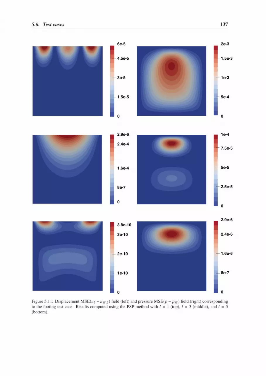
5.6. Test cases 137
6e-5
4.5e-5
3e-5
1.5e-5
0
2.9e-6
2.4e-4
1.6e-4
8e-7
0
3.8e-10
3e-10
2e-10
1e-10
0
2e-3
1.5e-3
1e-3
5e-4
0
1e-4
7.5e-5
5e-5
2.5e-5
0
2.9e-6
2.4e-6
1.6e-6
8e-7
0
Figure 5.11: Displacement MSE(u2 − uK ,2) field (left) and pressure MSE(p − pK ) field (right) correspondingto the footing test case. Results computed using the PSP method with l = 1 (top), l = 3 (middle), and l = 5(bottom).

138 Chapter 5. Poroelasticity with uncertain coefficients
Figure 5.12: Point injection test: Comparison between the total variance Var(u1(x, ξ )) and the sum of thefirst-order conditional variances
∑4i=1 Var(u1(x, ξ ) |ξi ) estimated using the PSP method with l = 5.
Figure 5.13: Point injection test: Conditional variances Var(u1(x, ξ ) |ξ1) (top left) Var(u1(x, ξ ) |ξ2) (top right)Var(u1(x, ξ ) |ξ3) (bottom left) Var(u1(x, ξ ) |ξ4) (bottom right) estimated using the PSP method with l = 5.
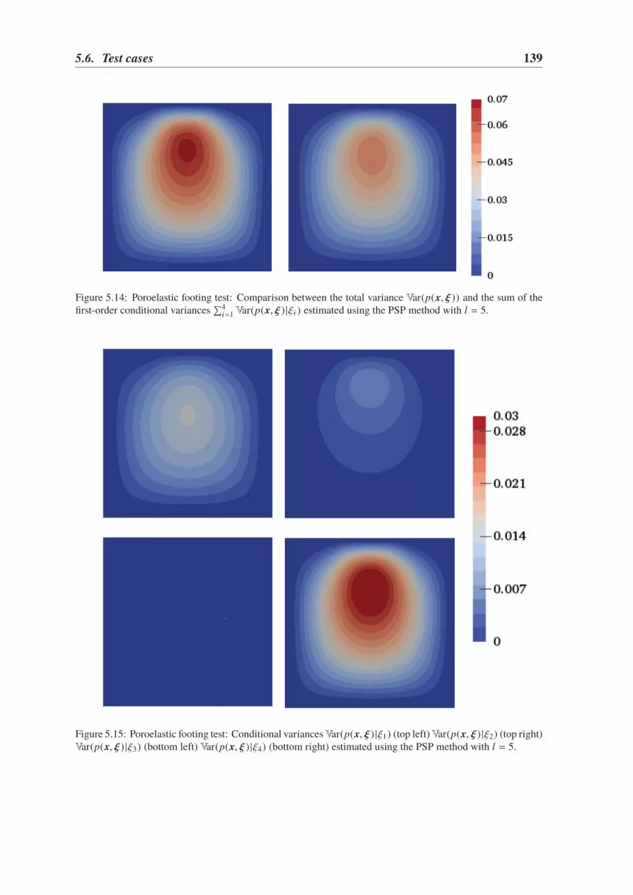
5.6. Test cases 139
Figure 5.14: Poroelastic footing test: Comparison between the total variance Var(p(x, ξ )) and the sum of thefirst-order conditional variances
∑4i=1Var(p(x, ξ ) |ξi ) estimated using the PSP method with l = 5.
Figure 5.15: Poroelastic footing test: Conditional variancesVar(p(x, ξ ) |ξ1) (top left)Var(p(x, ξ ) |ξ2) (top right)Var(p(x, ξ ) |ξ3) (bottom left) Var(p(x, ξ ) |ξ4) (bottom right) estimated using the PSP method with l = 5.

140 Chapter 5. Poroelasticity with uncertain coefficients
influence on the solutions is the hydraulic mobility κ (parametrized by ξ4), while the effect ofthe Biot–Willis coefficient α (parametrized by ξ3) on the variance is very weak. In particular,we notice in Figure 5.155.15 that α has no influence on the uncertainty of the pressure solving thefooting problem. Thus, in this case α could be fixed at a deterministic value. One possiblereason may be that the coefficient of variation cv(α) computed in (5.375.37) is smaller than theones relative to the other model coefficients. Finally, we remark that the conditional variancescorresponding to the Lamé’s coefficients µ, λ are almost the same in the case of the injectionproblem (cf. Figure 5.135.13), but are considerably different in the footing test (cf. Figure 5.155.15).
Appendix A
A nonconforming high-order method for
nonlinear poroelasticity
This appendix has been published in the following conference book (see [3434])
Finite Volumes for Complex Applications VIII,Hyperbolic, Elliptic and Parabolic Problems, 2017, Pages 537–545.
Contents
A.1 Introduction . . . . . . . . . . . . . . . . . . . . . . . . . . . . . . . . 141141
A.2 Mesh and notation . . . . . . . . . . . . . . . . . . . . . . . . . . . . . 142142
A.3 Discretization . . . . . . . . . . . . . . . . . . . . . . . . . . . . . . . . 143143
A.3.1 Nonlinear elasticity operator . . . . . . . . . . . . . . . . . . . . 143143
A.3.2 Darcy operator . . . . . . . . . . . . . . . . . . . . . . . . . . . 144144
A.3.3 Hydro-mechanical coupling . . . . . . . . . . . . . . . . . . . . 144144
A.4 Formulation of the method . . . . . . . . . . . . . . . . . . . . . . . . 145145
A.5 Numerical results . . . . . . . . . . . . . . . . . . . . . . . . . . . . . 146146
A.1 Introduction
We consider the nonlinear poroelasticity model obtained by generalizing the linear Biot’sconsolidation model of [2727, 190190] to nonlinear stress-strain constitutive laws. Our originalmotivation comes from applications in geosciences, where the support of polyhedral meshesand nonconforming interfaces is crucial.
Let Ω ⊂ Rd , d ∈ 2, 3, denote a bounded connected polyhedral domain with Lipschitzboundary ∂Ω and outward normal n. For a given finite time tF > 0, volumetric load f , fluidsource g, the considered nonlinear poroelasticity problem consists in finding a vector-valueddisplacement field u and a scalar-valued pore pressure field p solution of
−∇·σ (·,∇su ) + ∇p = f in Ω × (0, tF), (A.1a)
c0dt p + dt∇·u − ∇·(κ (·)∇p) = g in Ω × (0, tF), (A.1b)
141
142 Chapter A. A nonconforming high-order method for nonlinear poroelasticity
where ∇s denotes the symmetric gradient, c0 ≥ 0 is the constrained specific storage coeffi-cient, and κ : Ω→ (0, κ] is the scalar-valued permeability field. Equations (A.1aA.1a) and (A.1bA.1b)express, respectively, the momentum equilibrium and the fluid mass balance. For the sakeof simplicity, we assume that κ is piecewise constant on a partition PΩ of Ω into boundeddisjoint polyhedra and we consider the following homogeneous boundary conditions:
u = 0 on ∂Ω × (0, tF), (A.1c)
(κ (·)∇p) · n = 0 on ∂Ω × (0, tF). (A.1d)
The treatment of more general permeability fields and boundary conditions is possible upto minor modifications. Initial conditions are set prescribing u (·, 0) = u0 and, if c0 > 0,p(·, 0) = p0. In the incompressible case c0 = 0, we also need the following compatibilitycondition on g and zero-average constraint on p:
∫
Ω
g(·, t) = 0 and
∫
Ω
p(·, t) = 0 ∀t ∈ (0, tF).
We assume that the symmetric stress tensor σ : Ω × Rd×dsym → Rd×d
sym is a Caratheodoryfunction such that there exist real numbers σ, σ ∈ (0,+∞) and, for a.e. x ∈ Ω, and allτ, η ∈ Rd×d
sym , the following conditions hold:
‖σ (x, τ) − σ (x, 0)‖d×d ≤ σ ‖τ‖d×d, (growth) (A.2a)
σ (x, τ) : τ ≥ σ ‖τ‖2d×d, (coercivity) (A.2b)
(
σ (x, τ) − σ (x, η))
:(
τ − η) ≥ 0, (monotonicity) (A.2c)
where τ : η ≔∑d
i, j=1 τi, jηi, j and ‖τ‖2d×d= τ : τ.
A.2 Mesh and notation
Denote by H ⊂ R+∗ a countable set having 0 as unique accumulation point. We considerrefined mesh sequences (Th)h∈H where eachTh is a finite collection of disjoint open polyhedralelements T with boundary ∂T such that Ω =
⋃
T∈Th T and h = maxT∈Th hT with hT diameterof T . We assume that mesh regularity holds in the sense of [7676, Definition 1.38] and that,for all h ∈ H , Th is compatible with the partition PΩ, so that jumps of the permeabilitycoefficient do not occur inside mesh elements. Mesh faces are hyperplanar subsets of Ωwith positive (d−1)-dimensional Hausdorff measure and disjoint interiors. Interfaces arecollected in the set F i
h, boundary faces in F b
h, and we assume that Fh ≔ F i
h∪F b
his such that
⋃
T∈Th ∂T =⋃
F∈Fh F. For all T ∈ Th, FT ≔ F ∈ Fh : F ⊂ ∂T denotes the set of facescontained in ∂T and, for all F ∈ FT , nTF is the unit normal to F pointing out of T .
For X ⊂ Ω, we denote by ‖·‖X the norm in L2(X ;R), L2(X ;Rd), and L2(X ;Rd×d). Forl ≥ 0, the space Pl
d(X ;R) is spanned by the restriction to X of polynomials of total degree
l. On regular mesh sequences, we have the following optimal approximation property for theL2-projector πl
X: L1(X ;R) → Pl
d(X ;R): There exists Cap > 0 such that, for all h ∈ H , all
T ∈ Th, all s ∈ 1, . . . , l + 1, and all v ∈ H s (T ;R),
|v − πlTv |Hm (T ;R) ≤ Caphs−m
T |v |H s (T ;R) ∀m ∈ 0, . . . , s. (A.3)

A.3. Discretization 143
In what follows, for an integer l ≥ 0, we denote by Pld(Th;R), Pl
d(Th;Rd), and Pl
d(Th;Rd×d),
respectively, the space of scalar-, vector-, and tensor-valued broken polynomials of totaldegree l on Th. The space of broken vector-valued polynomials of total degree l on the meshskeleton is denoted by Pl
d(Fh;Rd).
A.3 Discretization
In this section we define the discrete counterparts of the elasticity and Darcy operators andof the hydro-mechanical coupling terms.
A.3.1 Nonlinear elasticity operator
The discretization of the nonlinear elasticity operator is based on the Hybrid High-Ordermethod of [7474]. Let a polynomial degree k ≥ 1 be fixed. The degrees of freedom (DOFs)for the displacement are collected in the space U k
h≔ P
kd(Th;Rd) × Pk
d(Fh;Rd). To account
for the Dirichlet condition (A.1cA.1c) we define the subspace
U kh,D ≔
v
h≔
(
(vT )T∈Th, (vF )F∈Fh) ∈ U k
h: vF = 0 ∀F ∈ F b
h
,
equipped with the discrete strain norm ‖ · ‖ǫ,h defined in (2.132.13). The DOFs corresponding to afunction v ∈ H1
0 (Ω;Rd) are obtained by means of the reduction map I kh
: H10 (Ω;Rd) → U k
h,D
such that I khv ≔
(
(πkTv )T∈Th, (π
kFv )F∈Fh
)
. Using the H1-stability of the L2-projector and thetrace inequality [7676, Lemma 1.49], we infer the existence of Cst > 0 independent of h suchthat, for all v ∈ H1
0 (Ω;Rd),
‖I khv ‖ǫ,h ≤ Cst‖v ‖H1(Ω;Rd ) . (A.4)
For all T ∈ Th, we denote byU kT
and I kT
the restrictions to T ofU kh
and I kh, and we define the
local symmetric gradient reconstruction Gks,T : U k
T→ Pk
d(T ;Rd×d
sym ) as the unique solution of
the pure traction problem: For a given vT=
(
vT, (vF )F∈FT) ∈ U k
T, find Gk
s,T vT∈ Pk
d(T ;Rd×d
sym )
such that, for all τ ∈ Pkd(T ;Rd×d
sym ),
∫
T
Gks,T vT
: τ = −∫
T
vT · (∇·τ) +∑
F∈FT
∫
F
vF · (τnTF ). (A.5)
The definition of Gks,T is justified by the commuting property (4.194.19) that, combined with (A.3A.3),
shows that Gks,T I k
Thas optimal approximation properties in Pk
d(T ;Rd×d
sym ). From Gks,T we define
the local displacement reconstruction operator r k+1T
: U kT→ Pk+1
d(T ;Rd) as in (2.52.5).
The discretization of the nonlinear elasticity operator is realized by the function ah :U k
h× U k
h→ R defined such that, for all w
h, v
h∈ U k
h,
ah(wh, v
h) ≔
∑
T∈Th
*.,∫
T
σ (·, Gks,TuT ) : Gk
s,T vT+
∑
F∈FT
γ
hF
∫
F
∆kTFuT · ∆
kTFvT
+/- , (A.6)

144 Chapter A. A nonconforming high-order method for nonlinear poroelasticity
where we penalize in a least-square sense the face-based residual ∆kT F
: U kT→ Pk
d(F;Rd)
such that, for all T ∈ Th, all vT∈ U k
T, and all F ∈ FT ,
∆kTFvT
≔ πkF (r k+1
T vT− vF ) − πk
T (r k+1T v
T− vT ).
This definition ensures that ∆kTF
vanishes whenever its argument is of the form I kTw with
w ∈ Pk+1d
(T ;Rd), a crucial property to obtain high-order error estimates (cf. Theorems 2.122.12,3.163.16, and 4.174.17). A possible choice for the scaling parameter γ > 0 in (A.6A.6) is γ = σ . For allv
h∈ U k
h,D, it holds (the proof follows from [7474, Lemma 4]):
C−1eq ‖vh
‖2ǫ,h ≤
∑
T∈Th
*.,‖Gks,T vT
‖2T +
∑
F∈FT
γ
hF
‖∆kTFvT
‖2F+/- ≤ Ceq‖vh
‖2ǫ,h,
where Ceq > 0 is independent of h. By (A.2bA.2b), this implies the coercivity of ah.
A.3.2 Darcy operator
The discretization of the Darcy operator is based on the Symmetric Weighted Interior Penaltymethod of [7777], cf. also [7676, Sec. 4.5]. At each time step, the discrete pore pressure is soughtin the broken polynomial space Pk
hdefined in (2.172.17). For all F ∈ F i
hand all qh ∈ Pk
d(Th;R),
we define the jump and average operators such that, denoting by qT and κT the restrictions ofqh and κ to an element T ∈ Th,
[qh]F ≔ qTF,1 − qTF,2, qhF ≔κTF,2
κTF,1+κTF,2qTF,1 +
κTF,1κTF,1+κTF,2
qTF,2,
where TF,1,TF,2 ∈ Th are such that F ⊂ TF,1∩TF,2. The bilinear form ch on Pkh×Pk
his defined
such that, for all qh, rh ∈ Pkh,
ch(rh, qh) ≔
∫
Ω
κ∇hrh · ∇hqh +
∑
F∈F ih
2ςκTF,1κTF,2hF (κTF,1+κTF,2 )
∫
F
[rh]F[qh]F
−∑
F∈F ih
∫
F
(
[rh]F κ∇hqhF + [qh]F κ∇hrhF) · nTF,1F,
(A.7)
where ∇h denotes the broken gradient and ς > 0 is a user-defined penalty parameter chosenlarge enough to ensure the coercivity of ch (cf. [7676, Lemma 4.51]). In the numerical tests ofSec. A.5A.5, we took ς = (N∂ +0.1)k2, with N∂ equal to the maximum number of faces betweenthe elements in Th. The fact that the boundary terms only appear on internal faces in (A.7A.7)reflects the Neumann boundary condition (A.1dA.1d).
A.3.3 Hydro-mechanical coupling
The hydro-mechanical coupling is realized by means of the bilinear form bh on U kh,D ×
Pkd(Th;R) such that, for all v
h∈ U k
h,D and all qh ∈ Pkd(Th;R),
bh(vh, qh) ≔ −
∑
T∈Th
∫
T
Gks,T vT
: qh |T I d,

A.4. Formulation of the method 145
where I d ∈ Rd×dsym is the identity matrix. A simple verification shows that there exists
Cbd > 0 independent of h such that bh(vh, qh) ≤ Cbd‖vh
‖ǫ,h‖qh‖Ω. Additionally, usingdefinition (A.5A.5) of Gk
s,T , it can be proved that, for all vh∈ U k
h,D, bh(vh, 1) = 0. The following
inf-sup condition expresses the stability of the coupling:Proposition A.1. There is a real β independent of h such that, for all qh ∈ Pk
d0(Th;R),
‖qh‖Ω ≤ β supvh∈Uk
h,D\0
bh(vh, qh)
‖vh‖ǫ,h
. (A.8)
Proof. Let qh ∈ Pkd0
(Th;R). There is vqh ∈ H10 (Ω;Rd) such that∇·vqh = qh and ‖vqh ‖H1(Ω;Rd ) ≤
Csj‖qh‖Ω, with Csj > 0 independent of h. Owing to (A.4A.4) we get
‖I khvqh ‖ǫ,h ≤ Cst‖vqh ‖H1(Ω;Rd ) ≤ CstCsj‖qh‖Ω.
Therefore, using the commuting property (4.194.19), denoting by S the supremum in (A.8A.8), andusing the previous inequality, it is inferred that
‖qh‖2Ω =
∑
T∈Th
∫
T
(∇svqh : qhI d) |T = −bh(I khvqh, qh) ≤ S‖I k
hvqh ‖ǫ,h ≤ CstCsjS‖qh‖Ω.
If a HHO discretization were used also for the Darcy operator, only cell DOFs would becontrolled by the inf-sup condition.
A.4 Formulation of the method
For the time discretization, we consider a uniform mesh of the time interval (0, tF) of stepτ ≔ tF/N with N ∈ N∗, and introduce the discrete times tn
≔ nτ for all 0 ≤ n ≤ N . For anyϕ ∈ Cl ([0, tF]; V ), we set ϕn
≔ ϕ(tn) ∈ V and let, for all 1 ≤ n ≤ N , δtϕn≔ (ϕn−ϕn−1)/τ ∈ V .
For all 1 ≤ n ≤ N , the discrete solution (unh, pn
h) ∈ U k
h,D × Pkh
at time tn is such that, for all
(vh, qh) ∈ U k
h,D × Pkd(Th;R),
ah(unh, vh
) + bh(vh, pn
h) =∑
T∈Th
∫
T
f n · vT,
c0
∫
Ω
(δt pnh)qh − bh(δtu
nh, qh) + ch(pn
h, qh) =
∫
Ω
gnqh.
(A.9)
If c0 = 0, we set the initial discrete displacement as u0h= I k
hu0. If c0 > 0, the usual way to
enforce the initial condition is to compute a displacement from the given initial pressure p0.We let p0
h≔ πk
hp0 and set u0
h∈ U k
h,D as the solution of
ah(u0h, vh
) =∑
T∈Th
∫
T
f 0 · vT − bh(vh, p0
h) ∀vh∈ U k
h,D.
At each time step n the discrete nonlinear equations (A.9A.9) are solved by the Newton’smethod using as initial guess the solution at step n − 1. At each Newton’s iteration theJacobian matrix is computed analytically and in the linearized system the displacementelement unknowns can be statically condensed (cf. Section 2.52.5).

146 Chapter A. A nonconforming high-order method for nonlinear poroelasticity
10´2
10´1.8
10´1.6
10´1.4
10´1.2
10´2
10´1
100
1
2
uNh ´ I
khu
N ǫ,h vs. h
pNh ´ πkhp
N Ω vs. h
10´2
10´1.8
10´1.6
10´1.4
10´1.2
10´2
10´1
1
2
uNh ´ I
khu
N ǫ,h vs. h
pNh ´ πkhp
N Ω vs. h
Figure A.1: Convergence tests on a Cartesian mesh family (left) and on a Voronoi mesh family (right).
A.5 Numerical results
We consider a regular exact solution in order to assess the convergence of the methodfor polynomial degree k = 1. Specifically, we solve problem (A.1A.1) in the square domainΩ = (0, 1)2 with tF = 1 and physical parameters c0 = 0 and κ = 1. As nonlinear constitutivelaw we take the Hencky–Mises relation given by
σ (∇su ) = (2 exp− dev(∇su ) −1) tr(∇su )I d + (4 − 2 exp− dev(∇su ))∇su,
where tr(τ) ≔ τ : I d and dev(τ) = tr(τ2)− 1d
tr(τ)2 are the trace and deviatoric operators. Itcan be checked that the previous stress-strain relation satisfies (A.2A.2). The exact displacementu and exact pressure p are given by
u (x, t) = t2 (
sin(πx1) sin(πx2), sin(πx1) sin(πx2))
,
p(x, t) = −π−1t(sin(πx1) cos(πx2) + cos(πx1) sin(πx2)).
The volumetric load f , the source term g, and the boundary conditions are inferred from theexact solutions. The time step τ on the coarsest mesh is 0.2 and it decreases with the meshsize h according to τ1/τ2 = 2h1/h2. In Fig. A.1A.1 we display the convergence results obtainedon two mesh families. The method exhibits second order convergence with respect to themesh size h for both the energy norm of the displacement and the L2-norm of the pressure atfinal time tF.

Appendix B
A posteriori error estimation for nonlinear
elasticity
This appendix has been published in the following peer-reviewed journal (see [3636])
Computational Methods in Applied Mathematics,Published online: 20 June 2018, DOI: 10.1515/cmam-2018-0012.
Contents
B.1 Introduction . . . . . . . . . . . . . . . . . . . . . . . . . . . . . . . . 147147
B.2 Setting . . . . . . . . . . . . . . . . . . . . . . . . . . . . . . . . . . . 149149
B.3 Equilibrated stress reconstruction . . . . . . . . . . . . . . . . . . . . 150150
B.3.1 Patchwise construction in the Arnold–Falk–Winther spaces . . . . 150150
B.3.2 Discretization and linearization error stress reconstructions . . . . 152152
B.4 A posteriori error estimate and adaptive algorithm . . . . . . . . . . . 154154
B.4.1 Guaranteed upper bound . . . . . . . . . . . . . . . . . . . . . . 154154
B.4.2 Adaptive algorithm . . . . . . . . . . . . . . . . . . . . . . . . . 156156
B.4.3 Local efficiency . . . . . . . . . . . . . . . . . . . . . . . . . . . 157157
B.5 Numerical results . . . . . . . . . . . . . . . . . . . . . . . . . . . . . 158158
B.5.1 L-shaped domain . . . . . . . . . . . . . . . . . . . . . . . . . . 158158
B.5.2 Notched specimen plate . . . . . . . . . . . . . . . . . . . . . . 161161
B.1 Introduction
In this appendix we develop equilibrated H (div)-conforming stress tensor reconstructions fora class of (linear and) nonlinear elasticity problems in the small deformation regime. Basedon these reconstructions, we can derive an a posteriori error estimate distinguishing thediscretization and linearization errors, as proposed in [9595] for nonlinear diffusion problems.Thanks to this distinction we can, at each iteration, compare these two error contributions
147
148 Chapter B. A posteriori error estimation for nonlinear elasticity
and stop the linearization algorithm once its contribution is negligible compared to thediscretization error.
Let Ω ∈ Rd , d ∈ 2, 3, be a bounded, simply connected polyhedron, which is occupiedby a body subjected to a volumetric force field f ∈ [L2(Ω)]d . For the sake of simplicity, weassume that the body is fixed on its boundary ∂Ω. The nonlinear elasticity problem consistsin finding a vector-valued displacement field u : Ω→ Rd solving
−∇·σ(∇su ) = f in Ω, (B.1a)
u = 0 on ∂Ω, (B.1b)
where∇su =12 ((∇u )T
+∇u ) denotes the symmetric gradient and expresses the strain tensorassociated to u . The stress-strain law σ : Ω × Rd×d
sym → Rd×dsym is assumed to satisfy regularity
requirements inspired by [3333, 6969]. Problem (B.1B.1) describes the mechanical behavior ofsoft materials [191191] and metal alloys [169169]. In these applications, the solution is oftenapproximated using H1-conforming finite elements. For nonlinear mechanical behavior laws,the resulting discrete nonlinear equation can then be solved using an iterative linearizationalgorithm yielding at each iteration a linear algebraic system to be solved, until the residualof the nonlinear equation lies under a predefined threshold.
The a posteriori error estimate is based on equilibrated stress reconstructions. It is wellknown that, in contrast to the analytical solution, the discrete stress tensor resulting fromthe conforming finite element method does not have continuous normal components acrossmesh interfaces, and that its divergence is not locally in equilibrium with the source termf on mesh elements. We consider here the stress reconstruction proposed in [175175] forlinear elasticity to restore these two properties. This reconstruction uses the Arnold–Falk–Winther mixed finite element spaces [77], leading to weakly symmetric tensors. In SectionB.3B.3 we apply this reconstruction to the nonlinear case by constructing two stress tensors:one playing the role of the discrete stress and one expressing the linearization error. Theyare obtained by summing up the solutions of minimization problems on cell patches aroundeach mesh vertex, so that they are H (div)-conforming and the sum of the two reconstructionsverifies locally the mechanical equilibrium (B.1aB.1a). The patch-wise equilibration techniquewas introduced in [3838, 6767] for the Poisson problem using the Raviart–Thomas finite elementspaces. In [8383] it is extended to linear elasticity without any symmetry constraint by usinglinewise Raviart–Thomas reconstructions. Elementwise reconstructions from local Neumannproblems requiring some pre-computations to determine the fluxes to obtain an equilibratedstress tensor can be found in [44, 5151, 134134, 161161], whereas in [158158] the direct prescription of thedegrees of freedom in the Arnold–Winther finite element space is considered.
Based on the equilibrated stress reconstructions, we develop the a posteriori error estimatein Section B.4B.4 and prove that it is efficient, meaning that, up to a generic constant, it is alsoa local lower bound for the error. The idea goes back to [170170] and was advanced amongstothers by [22, 132132, 133133, 172172] for the upper bound.Local lower error bounds are derived in [3838,6767, 9494, 9797, 144144]. Using equilibrated fluxes for a posteriori error estimation offers severaladvantages. The first one is, as mentioned above, the possible distinction of error componentsby expressing them in terms of fluxes. Secondly, the error upper bound is obtained withcomputable constants. In our case these constants depend only on the parameters of the
B.2. Setting 149
stress-strain relation. Thirdly, since the estimate is based on the discrete stress (and not thedisplacement), it does not depend on the mechanical behavior law (except for the constantin the upper bound). In addition, equilibrated error estimates were proven to be polynomial-degree robust for several linear problems in 2D, as the Poisson problem in [3737, 9797], linearelasticity in [8383] and the related Stokes problem in [4949] and recently in 3D in [9696].
The material is organized as follows. In Section B.2B.2 we introduce the weak and thediscrete formulations of problem (B.1B.1), along with some useful notation. In Section B.3B.3we present the equilibrated stress tensor reconstructions, first assuming that we solve thenonlinear discrete problem exactly, and then distinguish its discrete and its linearization errorpart at each iteration of a linearization solver. In Section B.4B.4 we derive the a posteriorierror estimate distinguishing the different error components. We then propose an algorithmequilibrating the error sources using adaptive stopping criteria for the linearization andadaptive remeshing. We finally show the efficiency of the error estimate. In Section B.5B.5 weevaluate the performance of the estimates. We perform a linear test with analytical solution inorder to compare the error estimator and the analytical error and to show that effectivity indicesare close to one. We then apply the proposed adaptive algorithm to application-oriented testswith nonlinear stress-strain relations.
B.2 Setting
In this section we write the weak and the considered discrete formulation of problem (B.1B.1).In the following, we will adopt the notation that bold greek letters are tensor-valued functionsand bold latin letters are vector-valued functions. For X ⊂ Ω, we respectively denoteby (·, ·)X and ‖·‖X the standard inner product and norm in L2(X ), with the conventionthat the subscript is omitted whenever X = Ω. The same notation is used in the vector-and tensor-valued cases. [H1(Ω)]d and H(div,Ω) stand for the Sobolev spaces composedof vector-valued [L2(Ω)]d functions with weak gradient in [L2(Ω)]d×d , and tensor-valued[L2(Ω)]d×d functions with weak divergence in [L2(Ω)]d , respectively. In what follows, weconsider stress-strain functions σ satisfying the following assumption.Assumption B.1 (Stress-strain relation). The symmetric stress tensor σ : Rd×d
sym → Rd×dsym is
continuous on Rd×dsym , satisfies the growth and strong monotonicity assumptions (3.2c3.2c) and
(3.40b3.40b), and σ (0) = 0.Multiplying (B.1aB.1a) by a test function v ∈ [H1
0 (Ω)]d and integrating by parts yields
(σ(∇su ),∇sv ) = ( f , v ). (B.2)
Owing to (3.2c3.2c), for all v, w ∈ [H1(Ω)]d , the form a(v, w ) ≔ (σ(∇sv ),∇sw ) is well definedand, from equation (B.2B.2), we can derive the following weak formulation of (B.1B.1):
Given f ∈ [L2(Ω)]d, find u ∈ [H10 (Ω)]d s.t., ∀v ∈ [H1
0 (Ω)]d, a(u, v ) = ( f , v ). (B.3)
From (B.3B.3) it is clear that the analytical stress tensor σ(∇su ) lies in the space Hs(div,Ω) ≔
τ ∈ [L2(Ω)]d×d | ∇·τ ∈ [L2(Ω)]d and τ is symmetric.The discretization of (B.3B.3) is based on a conforming triangulation Th of Ω, i.e. a set of
closed triangles or tetrahedra with union Ω and such that, for any distinct T1,T2 ∈ Th, the set

150 Chapter B. A posteriori error estimation for nonlinear elasticity
T1 ∩ T2 is either a common edge, a vertex, the empty set or, if d = 3, a common face. Theset of vertices of the mesh is denoted by Vh; it is decomposed into interior vertices V int
hand
boundary vertices Vexth
. For all a ∈ Vh, Ta is the patch of elements sharing the vertex a, ωa
the corresponding open subdomain in Ω and Va the set of vertices in ωa. For all T ∈ Th, VT
denotes the set of vertices of T , hT its diameter and nT its unit outward normal vector.For all p ∈ N and all T ∈ Th, we denote by Pp(T ) the space of d-variate polynomials
in T of total degree at most p and by Pp(Th) = ϕ ∈ L2(Ω) | ϕ|T ∈ Pp(T ) ∀T ∈ Ththe corresponding broken space over Th. In what follows we will focus on conformingdiscretizations of problem (B.2B.2) of polynomial degree p ≥ 2 to avoid numerical locking, cf[196196]. The discrete formulation reads: find uh ∈ [H1
0 (Ω)]d ∩ [Pp(Th)]d such that
∀vh ∈ [H10 (Ω)]d ∩ [Pp(Th)]d, a(uh, vh) = ( f , vh). (B.4)
This problem is usually solved using some iterative linearization algorithm defining at eachiteration k ≥ 1 a linear approximation σ k−1
lin of σ . Then the linearized formulation reads:find uk
h∈ [H1
0 (Ω)]d ∩ [Pp(Th)]d such that
∀vh ∈ [H10 (Ω)]d ∩ [Pp(Th)]d, (σ k−1
lin (∇sukh),∇svh) = ( f , vh). (B.5)
For the Newton algorithm the linearized stress σ k−1lin is defined, for all η ∈ Rd×d
sym , such that
σ k−1lin (η) ≔
∂σ (τ)
∂τ|τ=∇su
k−1h
(η − ∇suk−1h ) + σ(∇su
k−1h ).
B.3 Equilibrated stress reconstruction
In general, the discrete stress tensor σ(∇suh) resulting from (B.4B.4) does not lie in H(div,Ω)
and thus cannot verify the equilibrium equation (B.1aB.1a). In this section we will reconstructfrom σ(∇suh) a discrete stress tensor σh satisfying these properties. Based on this recon-struction, we then devise two equilibrated stress tensors representing the discrete stress and thelinearization error respectively, which will be useful for the distinction of error componentsin the a posteriori error estimate of Section B.4B.4.
B.3.1 Patchwise construction in the Arnold–Falk–Winther spaces
Let us for now suppose that uh solves (B.4B.4) exactly, before considering iterative linearizationmethods such as (B.5B.5) in Section B.3.2B.3.2. For the stress reconstruction we will use mixed finiteelement formulations on patches around mesh vertices in the spirit of [174174, 175175]. The goalis to obtain a stress tensor σh in a suitable (i.e. H (div)-conforming) finite element space bysumming up these local solutions. The local problems are posed such that this global stresstensor is close to the discrete stress tensor σ(∇suh) obtained from (B.4B.4), and that it satisfiesthe mechanical equilibrium on each element. In [174174] the stress tensor is reconstructed in theArnold–Winther finite element space [88], directly providing symmetric tensors, but requiringhigh computational effort. As done in [175175], we weaken the symmetry constraint and impose

B.3. Equilibrated stress reconstruction 151
Figure B.1: Element diagrams for (ΣT ,VT ,ΛT ) in the case d = q = 2
it weakly, as proposed in [77]: for each element T ∈ Th, the local Arnold–Falk–Winther mixedfinite element spaces of degree q ≥ 1 hinge on the Brezzi–Douglas–Marini mixed finiteelement spaces [4141] for each line of the stress tensor and are defined by
ΣT ≔ [Pq(T )]d×d, VT ≔ [Pq−1(T )]d, ΛT ≔ µ ∈ [Pq−1(T )]d×d | µ = −µT . (B.6)
For q = 2, the degrees of freedom are displayed in Figure B.1B.1. On a patchωa the global spaceΣh(ωa) is the subspace ofH(div, ωa) composed of functions belonging piecewise to ΣT . Thespaces Vh(ωa) and Λh(ωa) consist of functions lying piecewise in VT and ΛT respectively,with no continuity conditions between two elements.
Let now q ≔ p. On each patch we consider subspaces where a zero normal component isenforced on the stress tensor on the boundary of the patch, so that the sum of the local solutionswill have continuous normal component across any mesh interface. Since the boundarycondition (B.1bB.1b) prescribes the displacement and not the normal stress, we distinguish thecase whether a is an interior vertex or a boundary vertex. If a ∈ V int
hwe set
Σah ≔ τh ∈ Σh(ωa) | τhnωa
= 0 on ∂ωa,V a
h ≔ vh ∈ Vh(ωa) | (vh, z )ωa= 0 ∀z ∈ RMd ,
Λah ≔ Λh(ωa),
where RM2≔ b + c(x2,−x1)T | b ∈ R2, c ∈ R and RM3
≔ b + a × x | b ∈ R3, a ∈ R3are the spaces of rigid-body motions respectively for d = 2 and d = 3. If a ∈ Vext
hwe set
Σah ≔ τh ∈ Σh(ωa) | τhnωa
= 0 on ∂ωa\∂Ω,V a
h ≔ Vh(ωa),
Λah ≔ Λh(ωa).
For each vertex a ∈ Vh we define its hat function ψa ∈ P1(Th) as the piecewise linear functiontaking value one at the vertex a and zero on all other mesh vertices.Construction B.2 (Stress tensor reconstruction). Let uh solve (B.4B.4). For each a ∈ Vh find(σa
h, ra
h, λa
h) ∈ Σah× V a
h× Λa
h such that for all (τh, vh, µh) ∈ Σah× V a
h× Λa
h,
(σah, τh)ωa
+ (rah,∇·τh)ωa
+ (λah, τh)ωa
= (ψaσ(∇suh), τh)ωa, (B.7a)
(∇·σah, vh)ωa
= (−ψa f + σ(∇suh)∇ψa, vh)ωa, (B.7b)
(σah, µh)ωa
= 0. (B.7c)
Then, extending σah
by zero outside ωa, set σh ≔∑
a∈Vhσa
h.

152 Chapter B. A posteriori error estimation for nonlinear elasticity
For interior vertices, the source term in (B.7bB.7b) has to verify the Neumann compatibilitycondition
(−ψa f + σ(∇suh)∇ψa, z )ωa= 0 ∀z ∈ RMd . (B.8)
Taking ψa z as a test function in (B.4B.4), we see that (B.8B.8) holds and we obtain the followingresult.Lemma B.3 (Properties of σh). Let σh be prescribed by Construction B.2B.2. Then σh ∈H(div,Ω), and for all T ∈ Th, the following holds:
( f + ∇·σh, v )T = 0 ∀v ∈ VT ∀T ∈ Th. (B.9)
Proof. All the fields σah
are in H(div, ωa) and satisfy appropriate zero normal conditions sothat their zero-extension to Ω is in H(div,Ω). Hence, σh ∈ H(div,Ω). Let us prove (B.9B.9).Since (B.8B.8) holds for all a ∈ V int
h, we infer that (B.7bB.7b) is actually true for all vh ∈ Vh(ωa).
The same holds if a ∈ Vexth
by definition of V ah. Since Vh(ωa) is composed of piecewise
polynomials that can be chosen independently in each cell T ∈ Ta, and using σh |T =∑
a∈VTσa
h|T and the partition of unity
∑
a∈VTψa = 1, we infer that ( f +∇·σh, v )T = 0 for all
v ∈ VT and all T ∈ Th.
Remark B.4 (Choice of q). In contrast to flux reconstructions in the Raviart–Thomas space(cf. [3838] or [8383]), the choice q = p−1 in (B.6B.6) does not lead to optimal convergence rates of theresulting error estimate in Section B.4B.4. This is due to the fact that the Brezzi–Douglas–Marinispace is smaller than the Raviart–Thomas space of the same degree.
B.3.2 Discretization and linearization error stress reconstructions
Let now, for k ≥ 1, ukh
solve (B.5B.5). We will construct two different equilibrated H (div)-conforming stress tensors. The first one, σk
h,disc, represents as above the discrete stress
tensor σ(∇sukh), for which we will have to modify Construction B.2B.2, because the Neumann
compatibility condition (B.8B.8) is not satisfied anymore. The second stress tensor σkh,lin will be
a measure for the linearization error and approximate σ k−1lin (∇su
kh) − σ(∇su
kh). The matrix
resulting from the left side of (B.7B.7) will stay unchanged and we will only modify the sourceterms.
We denote by σ(∇sukh) the L2-orthogonal projection of σ(∇su
kh) onto [Pp−1(Th)]d×d
such that (σ(∇sukh) − σ(∇su
kh), τh) = 0 for any τh ∈ [Pp−1(Th)]d×d .
Construction B.5 (Discrete stress reconstruction). For each a ∈ Vh solve (B.7B.7) with ukh
instead of uh, σ(∇sukh) instead of σ(∇su
kh) and the source term in (B.7bB.7b) replaced by
−ψa f + σ(∇sukh)∇ψa − yk
disc,
where ykdisc ∈ RMd is the unique solution of
(ykdisc, z )ωa
= −( f , ψa z )ωa+ (σ(∇su
kh),∇s(ψa z ))ωa
∀z ∈ RMd . (B.10)

B.3. Equilibrated stress reconstruction 153
The so obtained problem reads: find (σah, ra
h, λa
h) ∈ Σah×V a
h×Λa
h such that for all (τh, vh, µh) ∈Σ
ah× V a
h× Λa
h,
(σah, τh)ωa
+ (rah,∇·τh)ωa
+ (λah, τh)ωa
= (ψaσ(∇sukh), τh)ωa
,
(∇·σah, vh)ωa
= (−ψa f + σ(∇sukh)∇ψa − yk
disc, vh)ωa,
(σah, µh)ωa
= 0.
Then set σkh,disc ≔
∑
a∈Vhσa
h.
Construction B.6 (Linearization error stress reconstruction). For each a ∈ Vh solve (B.7B.7)with uk
hinstead of uh, the source term in (B.7aB.7a) replaced by
ψa (σ k−1lin (∇su
kh) − σ(∇su
kh)),
and the source term in (B.7bB.7b) replaced by
(σ k−1lin (∇su
kh) − σ(∇su
kh))∇ψa + yk
disc,
where ykdisc ∈ RMd is defined by (B.10B.10). The corresponding local problem is to find
(σah, ra
h, λa
h) ∈ Σah× V a
h× Λa
h such that for all (τh, vh, µh) ∈ Σah× V a
h× Λa
h,
(σah, τh)ωa
+ (rah,∇·τh)ωa
+ (λah, τh)ωa
= (ψa (σ k−1lin (∇su
kh) − σ(∇su
kh)), τh)ωa
,
(∇·σah, vh)ωa
= ((σ k−1lin (∇su
kh) − σ(∇su
kh))∇ψa + yk
disc, vh)ωa,
(σah, µh)ωa
= 0.
Then set σkh,lin ≔
∑
a∈Vhσa
h.
Notice that the role of ykdisc is to guarantee that, for interior vertices, the source terms in
Constructions B.5B.5 and B.6B.6 satisfy the Neumann compatibility conditions
(−ψa f + σ(∇sukh)∇ψa − yk
disc, z )ωa= 0 ∀z ∈ RMd,
((σ k−1lin (∇su
kh) − σ(∇su
kh))∇ψa + yk
disc, z )ωa= 0 ∀z ∈ RMd .
Lemma B.7 (Properties of the discretization and linearization error stress reconstructions).Let σk
h,disc and σkh,lin be prescribed by Constructions B.5B.5 and B.6B.6. Then it holds
1. σkh,disc,σ
kh,lin ∈ H(div,Ω),
2. ( f + ∇·(σkh,disc + σ
kh,lin), v )T = 0 ∀v ∈ VT ∀T ∈ Th,
3. As the Newton solver converges, σkh,lin → 0.
Proof. The proof is similar to the proof of Lemma B.3B.3. The first property is again satisfieddue to the definition of Σa
h. In order to show that the second property holds, we add the two
equations (B.7bB.7b) obtained for each of the constructions. The right hand side of this sum thenreads (−ψa f + σ
k−1lin (∇su
kh)∇ψa, vh)ωa
. Once again we can, for any z ∈ RMd , take ψa z as
a test function in (B.5B.5) to show that this term is zero if vh ∈ RMd , and so the equation holdsfor all vh ∈ Vh(ωa). Then we proceed as in the proof of Lemma B.3B.3.

154 Chapter B. A posteriori error estimation for nonlinear elasticity
B.4 A posteriori error estimate and adaptive algorithm
In this section we first derive an upper bound on the error between the analytical solutionof (B.3B.3) and the solution uh of (B.4B.4), in which we then identify and distinguish the discretiza-tion and linearization error components at each Newton iteration for the solution uk
hof (B.5B.5).
Based on this distinction, we present an adaptive algorithm stopping the Newton iterationsonce the linearization error estimate is dominated by the estimate of the discretization error.Finally, we show the efficiency of the error estimate.
B.4.1 Guaranteed upper bound
We measure the error in the energy norm ‖v ‖2en ≔ a(v, v ) = (σ(∇sv ),∇sv ), for which we
obtain the propertiesσ2∗C
−2K ‖∇v ‖2 ≤ ‖v ‖2
en ≤ σ ‖∇sv ‖2, (B.13)
by applying (3.40b3.40b) and the Korn inequality for the left inequality, and the Cauchy–Schwarzinequality and (3.2c3.2c) for the right one. In our case it holds CK =
√2, owing to (B.1bB.1b).
Theorem B.8 (Basic a posteriori error estimate). Let u be the solution of (B.3B.3) and uh the
solution of (B.4B.4). Let σh be the stress tensor defined in Construction B.2B.2. Then,
‖u − uh‖en ≤√
2σσ−3∗
*.,∑
T∈Th
( hT
π‖ f + ∇·σh‖T + ‖σh − σ(∇suh)‖T
)2+/-1/2
. (B.14)
Remark B.9 (Constants σ and σ∗). For the estimate to be computable, the constants σ and σ∗have to be specified. For the linear elasticity model (3.33.3) we set σ ≔ 2µ+dλ and σ∗ ≔
√
2µ,whereas for the Hencky–Mises model (3.43.4) we set σ ≔ 2µ(0) + d λ(0) and σ∗ ≔
√
2µ(0).Following [175175], we obtain a sharper bound in the case of linear elasticity, with µ−1/2 insteadof√
2σσ−3∗ in (B.14B.14).
Proof of Theorem B.8B.8. We start by bounding the energy norm of the error by the dual normof the residual of the weak formulation (B.3B.3). Using (B.13B.13), (3.40b3.40b), the linearity of a in itssecond argument, and (B.3B.3) we obtain
‖u − uh‖2en ≤ σ ‖∇s(u − uh)‖2 ≤ σσ−2
∗ |a(u, u − uh) − a(uh, u − uh) |
= σσ−2∗ ‖∇(u − uh)‖
a(
u,u − uh
‖∇(u − uh)‖
)
− a
(
uh,u − uh
‖∇(u − uh)‖
) ≤ σσ−3
∗ CK ‖u − uh‖en supv∈[H1
0 (Ω)]d,‖∇v ‖=1
a(u, v ) − a(uh, v )
= σσ−3∗ CK ‖u − uh‖en sup
v∈[H10 (Ω)]d,‖∇v ‖=1
( f , v ) − (σ(∇suh),∇sv ).
and thus
‖u − uh‖en ≤ σσ−3∗ CK sup
v∈[H10 (Ω)]d,‖∇v ‖=1
( f , v ) − (σ(∇suh),∇sv ). (B.15)

B.4. A posteriori error estimate and adaptive algorithm 155
Note that, due to the symmetry of σ we can replace ∇sv by ∇v in the second term insidethe supremum. Now fix v ∈ [H1
0 (Ω)]d , such that ‖∇v ‖ = 1. Since σh ∈ H(div,Ω), we caninsert (∇·σh, v ) + (σh,∇v ) = 0 into the term inside the supremum and obtain
( f , v ) − (σ(∇suh),∇v ) = ( f + ∇·σh, v ) + (σh − σ(∇suh),∇v ). (B.16)
For the first term of the right hand side of (B.16B.16) we obtain, using (B.9B.9) on each T ∈ Th
to insert Π0Tv , which denotes the L2-projection of v onto [P0(T )]d , the Cauchy–Schwarz
inequality and the Poincaré inequality on simplices,
( f + ∇·σh, v ) ≤ ∑
T∈Th( f + ∇·σh, v −Π0
T v )T ≤
∑
T∈Th
hT
π‖ f + ∇·σh‖T ‖∇v ‖T, (B.17)
whereas the Cauchy–Schwarz inequality applied to the second term directly yields
(σh − σ(∇suh),∇v ) ≤ ∑
T∈Th‖σh − σ(∇suh)‖T ‖∇v ‖T .
Inserting in (B.15B.15) and applying again the Cauchy–Schwarz inequality yields the result.
The goal of the following result is to elaborate the error estimate (B.14B.14) so as to distinguishdifferent error components using the equilibrated stress tensors of Constructions B.5B.5 and B.6B.6.This distinction is essential for the development of Algorithm B.12B.12, where the mesh and thestopping criteria for the iterative solver are chosen adaptively. Notice that in Theorem B.8B.8 wedon’t necessarily need σh to be the stress tensor obtained in Construction B.2B.2. We only needit to satisfy two properties: First, equation (B.16B.16) requires σh to lie in H(div,Ω). Second,in order to be able to apply the Poincaré inequality in (B.17B.17), σh has to satisfy the localequilibrium relation
( f − ∇·σh, v )T = 0 ∀v ∈ [P0(T )]d ∀T ∈ Th.
Thus, the theorem also holds for σh ≔ σkh,disc +σ
kh,lin, where σk
h,disc and σkh,lin are defined in
Constructions B.5B.5.Theorem B.10 (A posteriori error estimate distinguishing different error sources). Let u be
the solution of (B.3B.3), ukh
the solution of (B.5B.5), and σh ≔ σkh,disc + σ
kh,lin. Then,
‖u − ukh‖en ≤
√2σσ−3
∗(
ηkdisc + η
klin + η
kquad + η
kosc
)
,
where the local discretization, linearization, quadrature and oscillation error estimators on
each T ∈ Th are defined as
ηkdisc,T ≔ ‖σk
h,disc − σ(∇sukh)‖T,
ηklin,T ≔ ‖σk
h,lin‖T,ηk
quad,T ≔ ‖σ(∇sukh) − σ(∇su
kh)‖T,
ηkosc,T ≔ hTπ
−1‖ f −Πp−1T
f ‖T,
with Πp−1T
denoting the L2-projection onto [Pp−1(T )]d , and for each error source the global
estimator is given by ηk· ≔ 2
(
∑
T∈Th (ηk·,T )2
)1/2.
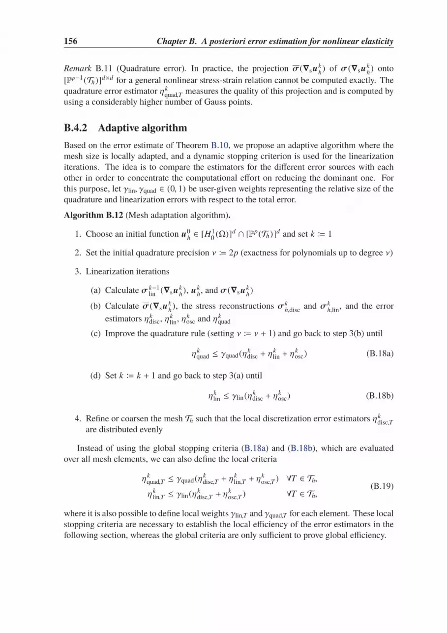
156 Chapter B. A posteriori error estimation for nonlinear elasticity
Remark B.11 (Quadrature error). In practice, the projection σ(∇sukh) of σ(∇su
kh) onto
[Pp−1(Th)]d×d for a general nonlinear stress-strain relation cannot be computed exactly. Thequadrature error estimator ηk
quad,T measures the quality of this projection and is computed byusing a considerably higher number of Gauss points.
B.4.2 Adaptive algorithm
Based on the error estimate of Theorem B.10B.10, we propose an adaptive algorithm where themesh size is locally adapted, and a dynamic stopping criterion is used for the linearizationiterations. The idea is to compare the estimators for the different error sources with eachother in order to concentrate the computational effort on reducing the dominant one. Forthis purpose, let γlin, γquad ∈ (0, 1) be user-given weights representing the relative size of thequadrature and linearization errors with respect to the total error.
Algorithm B.12 (Mesh adaptation algorithm).
1. Choose an initial function u0h∈ [H1
0 (Ω)]d ∩ [Pp(Th)]d and set k ≔ 1
2. Set the initial quadrature precision ν ≔ 2p (exactness for polynomials up to degree ν)
3. Linearization iterations
(a) Calculate σ k−1lin (∇su
kh), uk
h, and σ(∇su
kh)
(b) Calculate σ(∇sukh), the stress reconstructions σk
h,disc and σkh,lin, and the error
estimators ηkdisc, η
klin, ηk
osc and ηkquad
(c) Improve the quadrature rule (setting ν ≔ ν + 1) and go back to step 3(b) until
ηkquad ≤ γquad(ηk
disc + ηklin + η
kosc) (B.18a)
(d) Set k ≔ k + 1 and go back to step 3(a) until
ηklin ≤ γlin(ηk
disc + ηkosc) (B.18b)
4. Refine or coarsen the mesh Th such that the local discretization error estimators ηkdisc,T
are distributed evenly
Instead of using the global stopping criteria (B.18aB.18a) and (B.18bB.18b), which are evaluatedover all mesh elements, we can also define the local criteria
ηkquad,T ≤ γquad(ηk
disc,T + ηklin,T + η
kosc,T ) ∀T ∈ Th,
ηklin,T ≤ γlin(ηk
disc,T + ηkosc,T ) ∀T ∈ Th,
(B.19)
where it is also possible to define local weights γlin,T and γquad,T for each element. These localstopping criteria are necessary to establish the local efficiency of the error estimators in thefollowing section, whereas the global criteria are only sufficient to prove global efficiency.
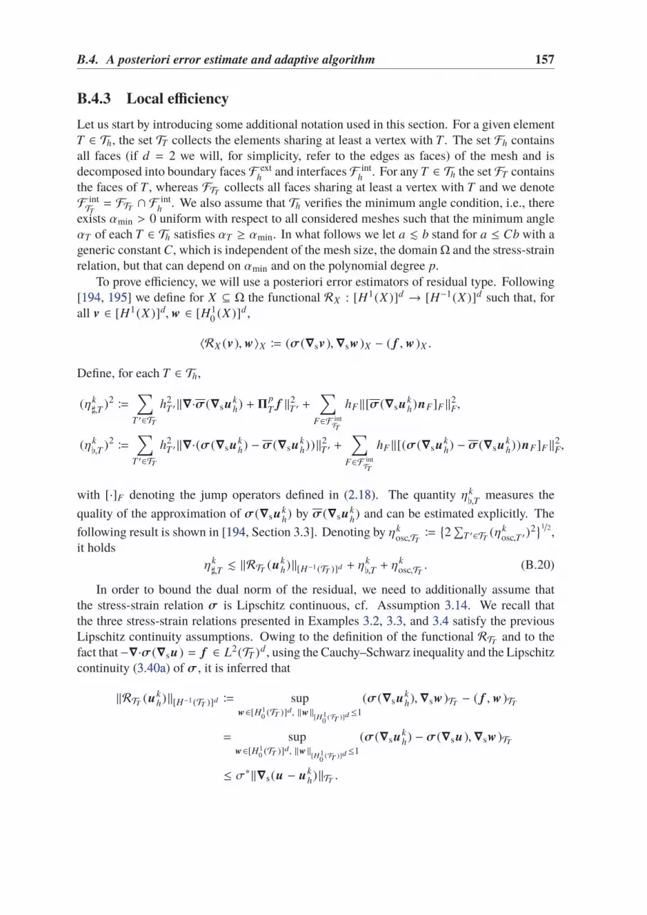
B.4. A posteriori error estimate and adaptive algorithm 157
B.4.3 Local efficiency
Let us start by introducing some additional notation used in this section. For a given elementT ∈ Th, the set TT collects the elements sharing at least a vertex with T . The set Fh containsall faces (if d = 2 we will, for simplicity, refer to the edges as faces) of the mesh and isdecomposed into boundary faces F ext
hand interfaces F int
h. For any T ∈ Th the set FT contains
the faces of T , whereas FTT collects all faces sharing at least a vertex with T and we denoteF intTT = FTT ∩ F
inth
. We also assume that Th verifies the minimum angle condition, i.e., thereexists αmin > 0 uniform with respect to all considered meshes such that the minimum angleαT of each T ∈ Th satisfies αT ≥ αmin. In what follows we let a . b stand for a ≤ Cb with ageneric constant C, which is independent of the mesh size, the domainΩ and the stress-strainrelation, but that can depend on αmin and on the polynomial degree p.
To prove efficiency, we will use a posteriori error estimators of residual type. Following[194194, 195195] we define for X ⊆ Ω the functional RX : [H1(X )]d → [H−1(X )]d such that, forall v ∈ [H1(X )]d, w ∈ [H1
0 (X )]d ,
〈RX (v ), w〉X ≔ (σ(∇sv ),∇sw )X − ( f , w )X .
Define, for each T ∈ Th,
(ηk♯,T
)2≔
∑
T ′∈TTh2
T ′‖∇·σ(∇sukh) +Π
p
Tf ‖2
T ′ +
∑
F∈F intTT
hF ‖[σ(∇sukh)nF]F ‖2
F,
(ηk,T )2
≔
∑
T ′∈TTh2
T ′‖∇·(σ(∇sukh) − σ(∇su
kh))‖2
T ′ +
∑
F∈F intTT
hF ‖[(σ(∇sukh) − σ(∇su
kh))nF]F ‖2
F,
with [·]F denoting the jump operators defined in (2.182.18). The quantity ηk,T
measures the
quality of the approximation of σ(∇sukh) by σ(∇su
kh) and can be estimated explicitly. The
following result is shown in [194194, Section 3.3]. Denoting by ηkosc,TT ≔
2∑
T ′∈TT (ηkosc,T ′)
21/2,it holds
ηk♯,T. ‖RTT (uk
h)‖[H−1(TT )]d + ηk,T + η
kosc,TT . (B.20)
In order to bound the dual norm of the residual, we need to additionally assume thatthe stress-strain relation σ is Lipschitz continuous, cf. Assumption 3.143.14. We recall thatthe three stress-strain relations presented in Examples 3.23.2, 3.33.3, and 3.43.4 satisfy the previousLipschitz continuity assumptions. Owing to the definition of the functional RTT and to thefact that−∇·σ(∇su ) = f ∈ L2(TT )d , using the Cauchy–Schwarz inequality and the Lipschitzcontinuity (3.40a3.40a) of σ , it is inferred that
‖RTT (ukh)‖[H−1(TT )]d ≔ sup
w∈[H10 (TT )]d, ‖w ‖
[H10
(TT )]d≤1
(σ(∇sukh),∇sw )TT − ( f , w )TT
= supw∈[H1
0 (TT )]d, ‖w ‖[H1
0(TT )]d
≤1
(σ(∇sukh) − σ(∇su ),∇sw )TT
≤ σ∗‖∇s(u − ukh)‖TT .

158 Chapter B. A posteriori error estimation for nonlinear elasticity
Thus, by (B.20B.20), the previous bound, and the strong monotonicity (3.40b3.40b) it holds
ηk♯,T. σ∗σ−1
∗ ‖u − ukh‖en,TT + η
k,T + η
kosc,TT
. (B.21)
It is well known that there exist nonconforming finite element methods which are equiva-lent to mixed finite element methods using the Brezzi–Douglas–Marini spaces (see e.g. [55]).Following the ideas of [9191, 9595, 118118] and references therein, we use these spaces to provethat ηk
disc,T . ηk♯,T
. As a result of this bound together with (B.21B.21), we obtain the followingTheorem (see [3636, Section 4.4] for the detailed proof).Theorem B.13 (Local efficiency). Let u ∈ [H1
0 (Ω)]d be the solution of (B.3B.3), ukh∈
[H10 (Ω)]d ∩ [Pp(Th)]d be arbitrary and σk
h,disc and σkh,lin defined by Constructions B.5B.5 and
B.6B.6. Let the local stopping criteria (B.19B.19) be verified. Then it holds for all T ∈ Th,
ηkdisc,T + η
klin,T + η
kquad,T + η
kosc,T . σ
∗σ−1∗ ‖u − uk
h‖en,TT + ηk,T + η
kosc,TT .
B.5 Numerical results
In this section we illustrate numerically our results on two test cases, both performed withthe Code_Aster11 software, which uses conforming finite elements of degree p = 2. Ourintention is, first, to show the relevance of the discretization error estimators used as meshrefinement indicators, and second, to propose a stopping criterion for the Newton iterationsbased on the linearization error estimator. All the triangulations are conforming, since in theremeshing progress hanging nodes are removed by bisecting the neighboring element.
B.5.1 L-shaped domain
Following [44, 129129, 158158], we consider the L-shaped domain Ω = (−1, 1)2 \ ([0, 1] × [−1, 0]),where for the linear elasticity case an analytical solution is given by
u (r, θ) =1
2µrα
(
cos(αθ) − cos((α − 2)θ)
A sin(αθ) + sin((α − 2)θ)
)
,
with the parameters
µ = 1.0, λ = 5.0, α = 0.6, A = 31/9.
This solution is imposed as Dirichlet boundary condition on ∂Ω, together with f = 0 in Ω.We perform this test for two different stress-strain relations. First on the linear elasticity model(3.33.3), where we can compare the error estimate (B.14B.14) to the analytical error ‖u − uh‖en.The second relation is the nonlinear Hencky–Mises model (3.43.4), for which we distinguishthe discretization and linearization error components and use the adaptive algorithm fromSection B.4.2B.4.2.
We compute the analytical error and its estimate on two series of unstructured meshes.Starting with the same initial mesh, we use uniform mesh refinement for the first one and
1http://web-code-aster.orghttp://web-code-aster.org

B.5. Numerical results 159
Figure B.2: L-shaped domain with linear elasticity model. Distribution of the error estimators (top) andthe analytical error (bottom) for the initial mesh (left) and after three (middle) and six (right) adaptive meshrefinements.
102 103
10−1.5
10−1
10−0.5
|Th | = number of mesh elements
error, unif.estimate, unif.error, adap.
estimate, adap.
|Th | Ieff
34 1.0084 1.01130 1.02
137 1.01214 1.05
239 1.01293 1.00429 1.01524 1.01
601 1.01801 1.011099 1.021142 1.02
Figure B.3: L-shaped domain with linear elasticity model. Left: Comparison of the error estimate (B.14B.14) and‖u − uh ‖en on two series of meshes, obtained by uniform and adaptive remeshing. Right: Effectivity indicesof the estimate for each mesh, with the meshes stemming from uniform refinement in italic.
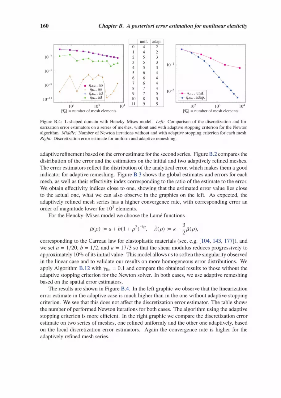
160 Chapter B. A posteriori error estimation for nonlinear elasticity
102 103 104
10−11
10−8
10−5
10−2
|Th | = number of mesh elements
ηdisc, noηlin, noηdisc, adηlin, ad
unif. adap.0 4 21 4 22 5 33 5 34 5 35 6 46 6 47 6 48 7 49 7 510 8 511 9 5
102 103 104
10−2
10−1
|Th | = number of mesh elements
ηdisc, unif.ηdisc, adap.
Figure B.4: L-shaped domain with Hencky–Mises model. Left: Comparison of the discretization and lin-earization error estimators on a series of meshes, without and with adaptive stopping criterion for the Newtonalgorithm. Middle: Number of Newton iterations without and with adaptive stopping criterion for each mesh.Right: Discretization error estimate for uniform and adaptive remeshing.
adaptive refinement based on the error estimate for the second series. Figure B.2B.2 compares thedistribution of the error and the estimators on the initial and two adaptively refined meshes.The error estimators reflect the distribution of the analytical error, which makes them a goodindicator for adaptive remeshing. Figure B.3B.3 shows the global estimates and errors for eachmesh, as well as their effectivity index corresponding to the ratio of the estimate to the error.We obtain effectivity indices close to one, showing that the estimated error value lies closeto the actual one, what we can also observe in the graphics on the left. As expected, theadaptively refined mesh series has a higher convergence rate, with corresponding error anorder of magnitude lower for 103 elements.
For the Hencky–Mises model we choose the Lamé functions
µ(ρ) ≔ a + b(1 + ρ2)−1/2, λ(ρ) ≔ κ − 3
2µ(ρ),
corresponding to the Carreau law for elastoplastic materials (see, e.g. [104104, 143143, 177177]), andwe set a = 1/20, b = 1/2, and κ = 17/3 so that the shear modulus reduces progressively toapproximately 10% of its initial value. This model allows us to soften the singularity observedin the linear case and to validate our results on more homogeneous error distributions. Weapply Algorithm B.12B.12 with γlin = 0.1 and compare the obtained results to those without theadaptive stopping criterion for the Newton solver. In both cases, we use adaptive remeshingbased on the spatial error estimators.
The results are shown in Figure B.4B.4. In the left graphic we observe that the linearizationerror estimate in the adaptive case is much higher than in the one without adaptive stoppingcriterion. We see that this does not affect the discretization error estimator. The table showsthe number of performed Newton iterations for both cases. The algorithm using the adaptivestopping criterion is more efficient. In the right graphic we compare the discretization errorestimate on two series of meshes, one refined uniformly and the other one adaptively, basedon the local discretization error estimators. Again the convergence rate is higher for theadaptively refined mesh series.

B.5. Numerical results 161
x
y
ǫ11
σ11
σc
E
Eres
Figure B.5: Left: Notched specimen plate. Right: Uniaxial traction curve
B.5.2 Notched specimen plate
In our second test we use the two nonlinear models of Examples 3.33.3 and 3.43.4 on a moreapplication-oriented test. The idea is to set a special sample geometry yielding to a modeldiscrimination test, namely different physical results for different models. We simulate theuniform traction of a notched specimen under plain strain assumption (cf. Figure B.5B.5).The notch is meant to favor strain localization phenomenon. We consider a domain Ω =(0, 10m) × (−10m, 10m) \ x ∈ R2 | ‖xm − (0, 11m)T ‖ ≤ 2m, we take f = 0, and weprescribe a displacement on the boundary leading to the following Dirichlet conditions:
ux = 0m if x = 0m, uy = −1.1 · 10−3m if y = −10m, uy = 1.1 · 10−3m if y = 10m.
In many applications, the information about the material properties are obtained in uniaxialexperiments, yielding a relation between σii and ǫ ii for a space direction xi. Since we onlyconsider isotropic materials, we can choose i = 1. From this curve one can compute thenonlinear Lamé functions of (3.43.4) and the damage function in (3.53.5). Although the uniaxialrelation is the same, the resulting stress-strain relations will be different. In our test, we usethe σ11 – ǫ11 – relation indicated in the right of Figure B.5B.5 with
σc = 3 · 104Pa, E =µ(3λ + 2µ)
λ + µ= 3 · 108Pa, Eres = 3 · 107Pa,
corresponding to the Lamé parameters µ = 326 · 109Pa and λ = 9
52 · 109Pa. For bothstress-strain relations we apply Algorithm B.12B.12 with γlin = 0.1. We first compare the resultsto a computation on a very fine mesh to evaluate the remeshing based on the discretizationerror estimators. Secondly, we perform adaptive remeshing based on these estimators butwithout applying the adaptive stopping of the Newton iterations and compare the two seriesof meshes. As in Section B.5.1B.5.1, we verify if the reduced number of iterations impacts thediscretization error.

162 Chapter B. A posteriori error estimation for nonlinear elasticity
Figure B.6: Notched specimen plate, comparison between Hencky–Mises (left in each picture) and damagemodel (right). Top left: tr(∇suh ). Top right: ηdisc on a fine mesh (no adaptive refinement). Bottom left: meshesafter six adaptive refinements. Bottom middle: initial mesh. Bottom right: ηdisc on the adaptively refinedmeshes.
Figure B.6B.6 shows the result of the first part of the test. In each of the four images the leftspecimen corresponds to the Hencky–Mises and the right to the isotropic damage model. Toillustrate the difference of the two models, the top left picture shows the trace of the straintensor. This scalar value is a good indicator for both models, representing locally the relativevolume increase which could correspond to either a damage or shear band localization zone.In the top right picture we see the distribution of the discretization error estimators in thereference computation (209,375 elements), whereas the distribution of the estimators onthe sixth adaptively refined mesh is shown in the bottom right picture (60,618 elements forHencky–Mises, 55,718 elements for the damage model). The corresponding meshes and theinitial mesh for the adaptive algorithm are displayed in the bottom left of the figure. To ensurea good discretization of the notch after repeated mesh refinement, the initial mesh cannotbe too corse in this curved area. We observe that the adaptively refined meshes match thedistribution of the discretization error estimators on the uniform mesh, and that the estimatorsare more evenly distributed on these meshes.
The results of the second part of the test are illustrated in Figure B.7B.7. As for the L-shape

B.5. Numerical results 163
103 104 10510−11
10−9
10−7
10−5
10−3
10−1
|Th | = number of mesh elements103 104
10−11
10−9
10−7
10−5
10−3
10−1
|Th | = number of mesh elements
ηdisc,noηlin,noηdisc, adηlin, ad
Hencky–Mises Damagenor. adap. nor. adap.
0 5 3 6 41 5 4 6 42 6 4 6 53 6 5 7 54 6 5 7 65 7 5 8 66 6 5 8 6
Figure B.7: Notched specimen plate. Comparison of the global discretization and linearization error estimatorswithout and with adaptive stopping criterion for the Hencky–Mises model (left) and the damage model (middle),and comparison of the number of performed Newton iterations (right).
test, we observe that the reduced number of Newton iterations does not affect the discretizationerror estimate, nor the overall error estimate which is dominated by the discretization errorestimate if the Newton algorithm is stopped.

164 Chapter B. A posteriori error estimation for nonlinear elasticity
List of Figures
1.1 Geologic storage of carbon dioxide in saline aquifers . . . . . . . . . . . . 22
1.2 Example of polyhedral mesh with degenerate elements in reservoir applications 1111
2.1 Triangular, hexagonal-dominant, Voronoi, and nonmatching quadrangularmeshes for the numerical tests. The triangular and nonmatching quadrangularmeshes were originally proposed for the FVCA5 benchmark [120120], whereasthe hexagonal-dominant mesh is the same used in [8080, Section 4.2.3]. . . . 4040
2.2 Errors vs. h . . . . . . . . . . . . . . . . . . . . . . . . . . . . . . . . . . 4141
2.3 Time convergence rate with BDF2, hexagonal mesh . . . . . . . . . . . . . 4242
2.4 Pressure field on the deformed domain at different times for the finest Carte-sian mesh containing 4,192 elements . . . . . . . . . . . . . . . . . . . . . 4343
2.5 Pressure profiles along the diagonal (0, 0)–(1, 1) of the domain for differentnormalized times t and meshes (k = 1). The time step is here τ = (2π/β) · 10−2. 4343
2.6 Pressure profiles along the diagonal (0, 0)–(1, 1) of the domain for κ = 1·10−6
and time step τ = 1 · 10−4. Small oscillations are present on the Cartesianmesh (left), whereas no sign of oscillations is present on the hexagonal mesh(right). . . . . . . . . . . . . . . . . . . . . . . . . . . . . . . . . . . . . . 4444
3.1 Local DOFs for k = 1 (left) and k = 2 (right). Shaded DOFs can belocally eliminated by static condensation when solving linearized versions ofproblem (3.213.21). . . . . . . . . . . . . . . . . . . . . . . . . . . . . . . . . 5656
3.2 Triangular, hexagonal-dominant, Voronoi, and nonmatching quadrangularmeshes for the numerical tests. The triangular and nonmatching quadrangularmeshes were originally proposed for the FVCA5 benchmark [120120]. The(predominantly) hexagonal was used in [8080]. The Voronoi mesh family wasobtained using the PolyMesher algorithm of [188188]. . . . . . . . . . . . . . 7070
3.3 Tensile test description and resulting stress components for the linear case.Values in 105Pa . . . . . . . . . . . . . . . . . . . . . . . . . . . . . . . . 7171
3.4 Shear test description and resulting stress components for the linear case.Values in 105Pa . . . . . . . . . . . . . . . . . . . . . . . . . . . . . . . . 7171
3.5 Tensile test case: Stress norm on the deformed domain. Values in 105Pa . . 7373
3.6 Shear test case: Stress norm on the deformed domain. Values in 104Pa . . . 7373
3.7 Energy vs h, tensile and shear test cases . . . . . . . . . . . . . . . . . . . 7575
165

166 List of Figures
5.1 Left: Scatter plot of 5000 realizations (µ, λ) for K ∼ U ([1, 20]) GPa andν ∼ U ([0.1, 0.4]). Right: Scatter plot of 5000 realizations (K, ν) for µ ∼U ([1, 10]) GPa and λ ∼ U ([2, 20]) GPa. . . . . . . . . . . . . . . . . . . 118118
5.2 Distribution of the bulk modulus K (left) and the Poisson ration ν (right) cor-responding to 106 realizations for µ ∼ U ([1, 10])GPa and λ ∼ U ([2, 20])GPa.119119
5.3 Distribution of 105 realizations of c0 obtained by solving (5.145.14) with uni-formly distributed random input coefficients λ, µ, and α. . . . . . . . . . . 120120
5.4 Examples of 1-D nested sequences including 1, 3, 5, and 9 quadrature points. 1281285.5 Examples of tensor-product quadrature grids for N = 2 and l = (3, 3).
In the full tensorization (top) the colored points correspond to the coloredcontributions in QFT
l= Q0 ⊗ Q3 + ∆
Q
1 ⊗ Q3 + ∆Q
2 ⊗ Q3 + ∆Q
3 ⊗ Q3. InSmolyak’s tensorization (bottom) the colored points correspond to the coloredcontributions in QL = Q0 ⊗ Q3 + ∆
Q
1 ⊗ Q2 + ∆Q
2 ⊗ Q1 + ∆Q
3 ⊗ Q0. . . . . . 1291295.6 Comparison of polynomials multi-index sets K (L) (below the red line) and
K ∗(L) (below the blue line) using a quadrature rule QL in d = 2 dimensions.Points are multi-indices (k1, k2) such F ∈ Pk1 ([0, 1]) × Pk1 ([0, 1]) is exactlyintegrated by QL . . . . . . . . . . . . . . . . . . . . . . . . . . . . . . . 131131
5.7 Pressure plotted on the deformed domain at t = tF = 1 (data are in KPa).Mean (Left) and Variance (Right) of the PSP method with level l = 5 andNp(l) = 2561. . . . . . . . . . . . . . . . . . . . . . . . . . . . . . . . . 133133
5.8 Pressure plotted on the deformed domain at t = 0.2. Mean (left) and Variance(right) computed using the PSP method with level l = 5 and Np(l) = 2561. 134134
5.9 Errors ‖MSE(u − uK )‖L2(D) and ‖MSE(p − pK )‖L2(D) vs. level l of theSparse Grid. Point injection test (left) and footing test (right) with modelcoefficients µ, λ, α, κ distributed according to (5.365.36). . . . . . . . . . . . . 135135
5.10 Displacement MSE(u1 − uK ,1) field (left) and pressure MSE(p − pK ) field(right) of the injection test case. Results are computed using the PSP methodwith l = 1 (top), l = 3 (middle), and l = 5 (bottom). . . . . . . . . . . . . 136136
5.11 Displacement MSE(u2 − uK ,2) field (left) and pressure MSE(p − pK ) field(right) corresponding to the footing test case. Results computed using thePSP method with l = 1 (top), l = 3 (middle), and l = 5 (bottom). . . . . . 137137
5.12 Point injection test: Comparison between the total variance Var(u1(x, ξ ))
and the sum of the first-order conditional variances∑4
i=1Var(u1(x, ξ ) |ξi)
estimated using the PSP method with l = 5. . . . . . . . . . . . . . . . . . 1381385.13 Point injection test: Conditional variancesVar(u1(x, ξ ) |ξ1) (top left)Var(u1(x, ξ ) |ξ2)
(top right) Var(u1(x, ξ ) |ξ3) (bottom left) Var(u1(x, ξ ) |ξ4) (bottom right) es-timated using the PSP method with l = 5. . . . . . . . . . . . . . . . . . . 138138
5.14 Poroelastic footing test: Comparison between the total varianceVar(p(x, ξ ))
and the sum of the first-order conditional variances∑4
i=1Var(p(x, ξ ) |ξi)
estimated using the PSP method with l = 5. . . . . . . . . . . . . . . . . . 1391395.15 Poroelastic footing test: Conditional variances Var(p(x, ξ ) |ξ1) (top left)
Var(p(x, ξ ) |ξ2) (top right) Var(p(x, ξ ) |ξ3) (bottom left) Var(p(x, ξ ) |ξ4)
(bottom right) estimated using the PSP method with l = 5. . . . . . . . . . 139139

List of Figures 167
A.1 Convergence tests on a Cartesian mesh family (left) and on a Voronoi meshfamily (right). . . . . . . . . . . . . . . . . . . . . . . . . . . . . . . . . 146146
B.1 Element diagrams for (ΣT,VT,ΛT ) in the case d = q = 2 . . . . . . . . . . 151151B.2 L-shaped domain with linear elasticity model. Distribution of the error
estimators (top) and the analytical error (bottom) for the initial mesh (left)and after three (middle) and six (right) adaptive mesh refinements. . . . . . 159159
B.3 L-shaped domain with linear elasticity model. Left: Comparison of the errorestimate (B.14B.14) and ‖u − uh‖en on two series of meshes, obtained by uniformand adaptive remeshing. Right: Effectivity indices of the estimate for eachmesh, with the meshes stemming from uniform refinement in italic. . . . . . 159159
B.4 L-shaped domain with Hencky–Mises model. Left: Comparison of thediscretization and linearization error estimators on a series of meshes, withoutand with adaptive stopping criterion for the Newton algorithm. Middle:
Number of Newton iterations without and with adaptive stopping criterionfor each mesh. Right: Discretization error estimate for uniform and adaptiveremeshing. . . . . . . . . . . . . . . . . . . . . . . . . . . . . . . . . . . . 160160
B.5 Left: Notched specimen plate. Right: Uniaxial traction curve . . . . . . . . 161161B.6 Notched specimen plate, comparison between Hencky–Mises (left in each
picture) and damage model (right). Top left: tr(∇suh). Top right: ηdisc
on a fine mesh (no adaptive refinement). Bottom left: meshes after sixadaptive refinements. Bottom middle: initial mesh. Bottom right: ηdisc onthe adaptively refined meshes. . . . . . . . . . . . . . . . . . . . . . . . . 162162
B.7 Notched specimen plate. Comparison of the global discretization and lin-earization error estimators without and with adaptive stopping criterion forthe Hencky–Mises model (left) and the damage model (middle), and com-parison of the number of performed Newton iterations (right). . . . . . . . 163163

168 List of Figures

Bibliography
[1] M. Abbas, A. Ern, and N. Pignet. Hybrid High-Order methods for finite
deformations of hyperelastic materials. Submitted. 2018.
[2] M. Ainsworth and J.T. Oden. “A posteriori error estimation in finite elementanalysis”. In: Pure and Applied Mathematics, Wiley-Interscience [John Wiley &
Sons], New York (2000).
[3] M. Ainsworth and J.T. Oden. “A posteriori error estimators for second order ellipticsystems Part 2. An optimal order process for calculating self-equilibrating fluxes”.In: Computers & Mathematics with Applications 26.9 (1993), pp. 75–87. doi:10.1016/0898-1221(93)90007-I10.1016/0898-1221(93)90007-I.
[4] M. Ainsworth and Rankin R. “Guaranteed computable error bounds for conformingand nonconforming finite element analysis in planar elasticity”. In: Internat. J.
Numer. Methods Engrg 82 (2010), pp. 1114–1157.
[5] T. Arbogast and Z. Chen. “On the implementation of mixed methods asnonconforming methods for second-order elliptic problems”. In: Math. Comp.
64.211 (1995), pp. 943–972.
[6] C.G. Armstrong, W.M. Lai, and V.C. Mow. “An analysis of the unconfinedcompression of articular cartilage”. In: J. Biomech. Eng. 106.2 (1984), pp. 165–173.
[7] D. N. Arnold, R. S. Falk, and R. Winther. “Mixed finite element methods for linearelasticity with weakly imposed symmetry”. In: Math. Comp. 76 (2007),pp. 1699–1723.
[8] D. N. Arnold and Winther R. “Mixed finite elements for elasticity”. In: Numer.
Math. 92 (2002), pp. 401–419.
[9] J.-L. Auriault and E. Sanchez-Palencia. “Étude du comportement macroscopiqued’un milieu poreux saturé déformable”. In: J. Méc. 16.4 (1977), pp. 575–603.
[10] I. Babuška and P. Chatzipantelidis. “On solving elliptic stochastic partial differentialequations”. In: Comput. Methods Appl. Mech. Engrg. 191.37 (2002),pp. 4093–4122. issn: 0045-7825. doi: 10.1016/S0045-7825(02)00354-710.1016/S0045-7825(02)00354-7.
[11] I. Babuška, F. Nobile, and R. Tempone. “A stochastic collocation method for ellipticpartial differential equations with random input data”. In: SIAM J. Numer. Anal.
45.3 (2007), pp. 1005–1034. doi: 10.1137/05064514210.1137/050645142.
169

170 Bibliography
[12] I. Babuška, R. Tempone, and G.E. Zouraris. “Galerkin Finite ElementApproximations of Stochastic Elliptic Partial Differential Equations”. In: SIAM J.
Numer. Anal. 42.2 (2004), pp. 800–825. issn: 0036-1429. doi:10.1137/S003614290241868010.1137/S0036142902418680.
[13] A. M. Barrientos, N. G. Gatica, and P. E. Stephan. “A mixed finite element methodfor nonlinear elasticity: two-fold saddle point approach and a-posteriori errorestimate”. In: Numer. Math. 91.2 (2002), pp. 197–222. doi:10.1007/s00211010033710.1007/s002110100337.
[14] S. Barry and G. Mercer. “Exact solution for two-dimensional time dependent flowand deformation within a poroelastic medium”. In: J. Appl. Mech. 66.2 (1999),pp. 536–540.
[15] S.I. Barry and G.K. Aldis. “Comparison of models for flow induced deformation ofsoft biological tissue”. In: J. Biomech. 23.7 (1990), pp. 647–654.
[16] F. Bassi, L. Botti, A. Colombo, D. A. Di Pietro, and P. Tesini. “On the flexibility ofagglomeration based physical space discontinuous Galerkin discretizations”. In: J.
Comput. Phys. 231.1 (2012), pp. 45–65.
[17] F. Bassi, S. Rebay, G. Mariotti, S. Pedinotti, and M. Savini. “A high-order accuratediscontinuous finite element method for inviscid and viscous turbomachineryflows”. In: Proceedings of the 2nd European Conference on Turbomachinery Fluid
Dynamics and Thermodynamics (1997), pp. 99–109.
[18] J. Bear. Dynamics of Fluids In Porous Media. Vol. 1. American Elsevier PublishingCompany, New York, 1972.
[19] L. Beirão Da Veiga. “A mimetic discretization method for linear elasticity”. In:M2AN Math. Model. Numer. Anal. 44.2 (2010), pp. 231–250.
[20] L. Beirão da Veiga, F. Brezzi, and L. D. Marini. “Virtual elements for linearelasticity problems”. In: SIAM J. Numer. Anal. 2.51 (2013), pp. 794–812.
[21] L. Beirão da Veiga, C. Lovadina, and D. Mora. “A Virtual Element Method forelastic and inelastic problems on polytope meshes”. In: Comput. Methods Appl.
Mech. Engrg. 295 (2015), pp. 327–346.
[22] E. Bemer, M. Boutéca, O. Vincké, N. Hoteit, and O. Ozanam. “Poromechanics:From linear to nonlinear poroelasticity and poroviscoelasticity”. In: Oil & Gas
Science and Technologies– Rev. IFP 56.6 (2001), pp. 531–544. doi:10.2516/OGST:200104310.2516/OGST:2001043.
[23] L. Berger, R. Bordas, D. Kay, and S. Tavener. “A stabilized finite element methodfor finite-strain three-field poroelasticity”. In: Comput. Mech. 60 (2017), pp. 51–68.doi: 10.1007/s00466-017-1381-810.1007/s00466-017-1381-8.
[24] A. Bespalov, C.E. Powell, and D. Silvester. “A priori error analysis of stochasticGalerkin mixed approximations of elliptic PDEs with random data”. In: SIAM J.
Numer. Anal. 50.4 (2012), pp. 2039–2063. doi: 10.1137/11085489810.1137/110854898.

Bibliography 171
[25] C. Bi and Y. Lin. “Discontinuous Galerkin method for monotone nonlinear ellipticproblems”. In: Int. J. Numer. Anal. Model 9 (2012), pp. 999–1024.
[26] S.O.R. Biabanaki, A.R. Khoei, and P. Wriggers. “Polygonal finite element methodsfor contact-impact problems on non-conformal meshes”. In: Comput. Meth. Appl.
Mech. Engrg. 269 (2014), pp. 198–221. doi: 10.1016/j.cma.2013.10.02510.1016/j.cma.2013.10.025.
[27] M. A. Biot. “General theory of threedimensional consolidation”. In: J. Appl. Phys.
12.2 (1941), pp. 155–164.
[28] M. A. Biot. “Nonlinear and semilinear rheology of porous solids”. In: J. Geoph.
Res. 78.23 (1973), pp. 4924–4937.
[29] M. A. Biot. “Theory of elasticity and consolidation for a porous anisotropic solid”.In: J. Appl. Phys. 26.2 (1955), pp. 182–185.
[30] D. Boffi, M. Botti, and D. A. Di Pietro. “A nonconforming high-order method forthe Biot problem on general meshes”. In: SIAM J. Sci. Comput. 38.3 (2016),A1508–A1537. doi: 10.1137/15M102550510.1137/15M1025505.
[31] D. Boffi, F. Brezzi, and M. Fortin. Mixed finite element methods and applications.Vol. 44. Springer Series in Computational Mathematics. Berlin Heidelberg:Springer, 2013. doi: 10.1007/978-3-642-36519-510.1007/978-3-642-36519-5.
[32] L. Botti, D. A. Di Pietro, and J. Droniou. A Hybrid High-Order discretisation of the
Brinkman problem robust in the Darcy and Stokes limits. Submitted. Mar. 2018.url: http://hal.archives-ouvertes.fr/hal-01746367http://hal.archives-ouvertes.fr/hal-01746367.
[33] M. Botti, D. A. Di Pietro, and P. Sochala. “A Hybrid High-Order method fornonlinear elasticity”. In: SIAM J. Numer. Anal. 55.6 (2017), pp. 2687–2717. doi:10.1137/16M110594310.1137/16M1105943.
[34] M. Botti, D. A. Di Pietro, and P. Sochala. “A nonconforming high-order method fornonlinear poroelasticity”. In: Finite Volumes for Complex Applications VIII –
Hyperbolic, Elliptic and Parabolic Problems. 2017, pp. 537–545.
[35] M. Botti, D. A. Di Pietro, and P. Sochala. Analysis of a Hybrid
High-Order–discontinuous Galerkin discretization method for nonlinear
poroelasticity. Submitted. May 2018. url:http://hal.archives-ouvertes.fr/hal-01785810http://hal.archives-ouvertes.fr/hal-01785810.
[36] M. Botti and R. Riedlbeck. “Equilibrated stress tensor reconstruction and aposteriori error estimation for nonlinear elasticity”. In: Comput. Methods Appl.
Math. (June 2018). doi: 10.1515/cmam-2018-001210.1515/cmam-2018-0012.
[37] D. Braess, V. Pillwein, and J. Schöberl. “Equilibrated residual error estimates arep-robust”. In: Comput. Methods Appl. Mech. Engrg. 198 (2009), pp. 1189–1197.
[38] D. Braess and J. Schöberl. “Equilibrated residual error estimator for edge elements”.In: Math. Comp. 77.262 (2008), pp. 651–672.
[39] S. C. Brenner. “Korn’s inequalities for piecewise H1 vector fields”. In: Math. Comp.
73.247 (2004), pp. 1067–1087. issn: 0025-5718.

172 Bibliography
[40] H. Brezis. Functional Analysis, Sobolev Spaces and Partial Differential Equations.Universitext. Springer New York, 2010. isbn: 9780387709130.
[41] F. Brezzi, J. Douglas, and L. D. Marini. “Recent results on mixed finite elementmethods for second order elliptic problems”. In: Vistas in applied mathematics.
Numerical analysis, atmospheric sciences, immunology. Ed. byDorodnitsyn Balakrishnan and Lions Eds. Optimization Software Inc., PublicationsDivision, New York, 1986, pp. 25–43.
[42] F. Brezzi, G. Manzini, L. D. Marini, P. Pietra, and A. Russo. “DiscontinuousGalerkin approximations for elliptic problems”. In: Numer. Methods Partial
Differential Equations 16.4 (2000), pp. 365–378. issn: 0749-159X.
[43] M. K. Brun, I. Berre, J. M. Nordbotten, and F. A. Radu. “Upscaling of the Couplingof Hydromechanical and Thermal Processes in a Quasi-static Poroelastic Medium”.In: Transport in Porous Media 124.1 (2018), pp. 137–158. issn: 1573-1634. doi:10.1007/s11242-018-1056-810.1007/s11242-018-1056-8.
[44] H. Bryne and L. Preziosi. “Modeling tumour growth using the theory of mixtures”.In: Mathematical Medicine and Biology 20.4 (2003), pp. 341–366.
[45] R. Burridge and Keller J. B. “Poroelasticity equations derived from microstructure”.In: J. Acoust. Soc. Am. 70.4 (1981), pp. 1140–1146. doi: 10.1121/1.38694510.1121/1.386945.
[46] R. H. Cameron and W. T. Martin. “The orthogonal development of nonlinearfunctionals in series of Fourier–Hermite functionals”. In: Ann. Math. 48 (1947),pp. 385–392.
[47] A. Cangiani, E. H. Georgoulis, and P. Houston. “hp-version discontinuous Galerkinmethods on polygonal and polyhedral meshes”. In: Math. Models Methods Appl.
Sci. 24.10 (2014), pp. 2009–2041. issn: 0218-2025. doi:10.1142/S021820251450014610.1142/S0218202514500146.
[48] Y. Cao, S. Chen, and A. J. Mier. “Analysis and numerical approximations ofequations of nonlinear poroelasticity”. In: Discrete & Continuous Dynamical
Systems - B 18 (2013), pp. 1253–1273. doi: 10.3924/dcdsb.2013.18.125310.3924/dcdsb.2013.18.1253.
[49] M. Čermák, F. Hecht, Z. Tang, and M. Vohralík. “Adaptive inexact iterativealgorithms based on polynomial-degree-robust a posteriori estimates for the Stokesproblem”. In: Numer. Math. 138.4 (2018), pp. 1027–1065. doi:10.1007//s00211-017-0925-310.1007//s00211-017-0925-3.
[50] M. Cervera, M. Chiumenti, and R. Codina. “Mixed stabilized finite elementmethods in nonlinear solid mechanics: Part II: Strain localization”. In: Comput.
Methods in Appl. Mech. and Engrg. 199.37–40 (2010), pp. 2571–2589. doi:10.1016/j.cma.2010.04.00510.1016/j.cma.2010.04.005.
[51] L. Chamoin, P. Ladevèze, and F. Pled. “On the techniques for constructingadmissible stress fields in model verification: Performances on engineeringexamples”. In: Internat. J. Numer. Methods Engrg. 88.5 (2011), pp. 409–441. doi:10.1002/nme.318010.1002/nme.3180.

Bibliography 173
[52] C.S. Chang. “Uncertainty in one-dimensional consolidation analysis”. In: J.
Geothec. Eng. 111.12 (1985), pp. 1411–1424.
[53] J. Charrier. “Strong and weak error estimates for elliptic partial differentialequations with random coefficients”. In: SIAM J. Numer. Anal. 50.1 (2012),pp. 216–246. doi: 10.1137/10080053110.1137/100800531.
[54] H. Chi, L. Beirão da Veiga, and G.H. Paulino. “Some basic formulations of thevirtual element method (VEM) for finite deformations”. In: Computer Methods in
Applied Mechanics and Engineering 318 (2017), pp. 148–192. issn: 0045-7825.doi: 10.1016/j.cma.2016.12.02010.1016/j.cma.2016.12.020.
[55] H. Chi, C. Talischi, O. Lopez-Pamies, and G. H. Paulino. “Polygonal finite elementsfor finite elasticity”. In: Int. J. Numer. Methods Eng. 101.4 (2015), pp. 305–328.issn: 1097-0207. doi: 10.1002/nme.480210.1002/nme.4802.
[56] P. G. Ciarlet and P. Ciarlet. “Another approach to linearized elasticity and a newproof of Korn’s inequality”. In: Math. Models Methods Appl. Sci. 15.02 (2005),pp. 259–271. doi: 10.1142/S021820250500035210.1142/S0218202505000352.
[57] B. Cockburn, D. A. Di Pietro, and A. Ern. “Bridging the Hybrid High-Order andHybridizable Discontinuous Galerkin Methods”. In: M2AN Math. Model. Numer.
Anal. (2015). Published online. DOI 10.1051/m2an/201505110.1051/m2an/2015051.
[58] P. R. Conrad and Y. M. Marzouk. “Adaptive Smolyak PseudospectralApproximations”. In: SIAM J. Sci. Comp. 35.6 (2013), A2643–A2670. doi:10.1137/12089071510.1137/120890715.
[59] P. G. Constantine, M. S. Eldred, and E. T. Phipps. “Sparse pseudospectralapproximation method”. In: Comput. Methods Appl. Mech. Engrg. 229 (2012),pp. 1–12.
[60] P. Cosenza, M. Ghoreychi, G. De Marsily, G. Vasseur, and S. Violette. “Theoreticalprediction of poroelastic properties of argillaceous rocks from in situ specificstorage coefficient”. In: Water Resour. Res. 38.10 (2002), p. 1207. doi:10.1029/2001WR00120110.1029/2001WR001201.
[61] O. Coussy. Poromechanics. J. Wiley and Sons, ltd., 2004. doi:10.1002/047009271810.1002/0470092718.
[62] A.A. Darrag and M.A Tawil. “The consolidation of soils under stochastic initialexcess pore pressure”. In: Applied Mathematical Modelling 17.11 (1993),pp. 609–612. doi: 10.1016/0307-904X(93)90069-S10.1016/0307-904X(93)90069-S.
[63] R. Davies, G. Foulger, A. Bindley, and P. Styles. “Induced seismicity and hydraulicfracturing for the recovery of hydrocarbons”. In: Mar. Petrol. Geol. 45.1 (2013),pp. 171–185. doi: 10.1016/j.marpetgeo.2013.03.01610.1016/j.marpetgeo.2013.03.016.
[64] K. Deimling. “Nonlinear functional analysis”. In: Springer-Verlag, Berlin (1985).doi: 10.1007/978-3-662-00547-710.1007/978-3-662-00547-7.

174 Bibliography
[65] P. Delgado and V. Kumar. “A stochastic Galerkin approach to uncertaintyquantification in poroelastic media”. In: Applied Mathematics and Computation
266.1 (2015), pp. 328–338. doi: 10.1016/j.amc.2015.04.12710.1016/j.amc.2015.04.127.
[66] M. Destrade and R. W. Ogden. “On the third- and fourth-order constants ofincompressible isotropic elasticity”. In: The Journal of the Acoustical Society of
America 128.6 (2010), pp. 3334–3343. doi: 10.1121/1.350510210.1121/1.3505102.
[67] P. Destuynder and B. Métivet. “Explicit error bounds in a conforming finite elementmethod”. In: Math. Comp. 68.228 (1999), pp. 1379–1396.
[68] E. Detournay and A. H. D. Cheng. “Fundamentals of poroelasticity”. In:Comprehensive rock engineering. Vol. 2. Ed. by J.A. Hudson. Pergamon, 1993,pp. 113–171.
[69] D. A. Di Pietro and J. Droniou. “A Hybrid High-Order method for Leray–Lionselliptic equations on general meshes”. In: Math. Comp. 86.307 (2017),pp. 2159–2191. doi: 10.1142/S021820251750019110.1142/S0218202517500191.
[70] D. A. Di Pietro and J. Droniou. “W s,p-approximation properties of ellipticprojectors on polynomial spaces, with application to the error analysis of a HybridHigh-Order discretization of Leray–Lions problems”. In: Math. Models Methods
Appl. Sci. 27.5 (2017), pp. 879–908. doi: 10.1142/S021820251750019110.1142/S0218202517500191.
[71] D. A. Di Pietro, J. Droniou, and A. Ern. “A Discontinuous-Skeletal Method forAdvection-Diffusion-Reaction on General Meshes”. In: SIAM J. Numer. Anal. 53.5(2015), pp. 2135–2157. doi: 10.1137/14099397110.1137/140993971.
[72] D. A. Di Pietro, J. Droniou, and G. Manzini. “Discontinuous Skeletal GradientDiscretisation methods on polytopal meshes”. In: J. Comput. Phys. 355 (2018),pp. 397–425. doi: 10.1016/j.jcp.2017.11.01810.1016/j.jcp.2017.11.018.
[73] D. A. Di Pietro and A. Ern. “A family of arbitrary order mixed methods forheterogeneous anisotropic diffusion on general meshes”. In: IMA J. Numer. Anal.
(2016). Published online. DOI: 10.1093/imanum/drw00310.1093/imanum/drw003.
[74] D. A. Di Pietro and A. Ern. “A hybrid high-order locking-free method for linearelasticity on general meshes”. In: Comput. Meth. Appl. Mech. Engrg. 283 (2015),pp. 1–21. doi: 10.1016/j.cma.2014.09.00910.1016/j.cma.2014.09.009.
[75] D. A. Di Pietro and A. Ern. “Discrete functional analysis tools for discontinuousGalerkin methods with application to the incompressible Navier–Stokes equations”.In: Math. Comp. 79 (2010), pp. 1303–1330. doi:10.1090/S0025-5718-10-02333-110.1090/S0025-5718-10-02333-1.
[76] D. A. Di Pietro and A. Ern. Mathematical aspects of discontinuous Galerkin
methods. Vol. 69. Mathématiques & Applications. Berlin: Springer-Verlag, 2012.doi: 10.1007/978-3-642-22980-010.1007/978-3-642-22980-0.
[77] D. A. Di Pietro, A. Ern, and J.-L. Guermond. “Discontinuous Galerkin methods foranisotropic semi-definite diffusion with advection”. In: SIAM J. Numer. Anal. 46.2(2008), pp. 805–831. doi: 10.1137/06067610610.1137/060676106.

Bibliography 175
[78] D. A. Di Pietro, A. Ern, and S. Lemaire. “An arbitrary-order and compact-stencildiscretization of diffusion on general meshes based on local reconstructionoperators”. In: Comput. Methods Appl. Math. 14.4 (2014), pp. 461–472.
[79] D. A. Di Pietro, B. Kapidani, R. Specogna, and F. Trevisan. “An Arbitrary-OrderDiscontinuous Skeletal Method for Solving Electrostatics on General PolyhedralMeshes”. In: IEEE Transactions on Magnetics 53.6 (June 2017), pp. 1–4. issn:0018-9464. doi: 10.1109/TMAG.2017.266654610.1109/TMAG.2017.2666546.
[80] D. A. Di Pietro and S. Lemaire. “An extension of the Crouzeix–Raviart space togeneral meshes with application to quasi-incompressible linear elasticity and Stokesflow”. In: Math. Comp. 84.291 (2015), pp. 1–31.
[81] D. A. Di Pietro and S. Nicaise. “A locking-free discontinuous Galerkin method forlinear elasticity in locally nearly incompressible heterogeneous media”. In: Appl.
Numer. Math. 63 (2013), pp. 105–116. issn: 0168-9274. doi:10.1016/j.apnum.2012.09.00910.1016/j.apnum.2012.09.009.
[82] D. A. Di Pietro and R. Tittarelli. “Numerical Methods for PDEs. State of the ArtTechniques”. In: ed. by L. Formaggia D. A. Di Pietro A. Ern. SEMA-SIMAI 15.Springer, 2018. Chap. An introduction to Hybrid High-Order methods. url:http://arxiv.org/abs/1703.05136http://arxiv.org/abs/1703.05136.
[83] P. Dörsek and J. Melenk. “Symmetry-free, p-robust equilibrated error indication forthe hp-version of the FEM in nearly incompressible linear elasticity”. In: Comput.
Methods Appl. Math. 13 (2013), pp. 291–304.
[84] J. Droniou. “Finite volume schemes for fully non-linear elliptic equations indivergence form”. In: ESAIM: Mathematical Modelling and Numerical Analysis -
Modélisation Mathématique et Analyse Numérique 40.6 (2006), pp. 1069–1100.
[85] J. Droniou, R. Eymard, T. Gallouët, C. Guichard, and R. Herbin. The gradient
discretisation method. Preprint hal-01366646hal-01366646. Nov. 2016.
[86] J. Droniou, R. Eymard, T. Gallouët, C. Guichard, and R. Herbin. The gradient
discretisation method: A framework for the discretisation and numerical analysis of
linear and nonlinear elliptic and parabolic problems. Maths & Applications. Toappear. Springer, 2017, 509p. url:https://hal.archives-ouvertes.fr/hal-01382358https://hal.archives-ouvertes.fr/hal-01382358.
[87] J. Droniou and B. P. Lamichhane. “Gradient Schemes for Linear and Non-linearElasticity Equations”. In: Numer. Math. 129.2 (2015), pp. 251–277. issn:0029-599X. doi: 10.1007/s00211-014-0636-y10.1007/s00211-014-0636-y.
[88] T. Dupont and R. Scott. “Polynomial approximation of functions in Sobolevspaces”. In: Math. Comp. 34.150 (1980), pp. 441–463.
[89] G. Duvaut and Lions J.L. Inequalities in Mechanics and Physics. 1st ed.Grundlehren der mathematischen Wissenschaften 219. Springer-Verlag BerlinHeidelberg, 1976. isbn: 978-3-642-66167-9,978-3-642-66165-5.

176 Bibliography
[90] W. Ehlers and G. Eipper. “Finite Elastic Deformations in Liquid-Saturated andEmpty Porous Solids”. In: Transport in Porous Media 34.1 (1999), pp. 179–191.issn: 1573-1634. doi: 10.1023/A:100656550909510.1023/A:1006565509095.
[91] L. El Alaoui, A. Ern, and M. Vohralík. “Guaranteed and robust a posteriori errorestimates and balancing discretization and linearization errors for monotonenonlinear problems”. In: Comput. Methods Appl. Mech. Engrg. 200 (2011),pp. 2782–2795.
[92] A. Ern and J.-L. Guermond. Theory and Practice of Finite Elements. Vol. 159.Applied Mathematical Sciences. New York, NY: Springer-Verlag, 2004.
[93] A. Ern, A. F. Stephansen, and P. Zunino. “A discontinuous Galerkin method withweighted averages for advection-diffusion equations with locally small andanisotropic diffusivity”. In: IMA J. Numer. Anal. 29.2 (2009), pp. 235–256. issn:0272-4979. doi: 10.1093/imanum/drm05010.1093/imanum/drm050.
[94] A. Ern and M. Vohralík. “A posteriori error estimation based on potential and fluxreconstruction for the heat equation”. In: SIAM J. Numer. Anal. 48.1 (2010),pp. 198–223.
[95] A. Ern and M. Vohralík. “Adaptive inexact Newton methods with a posterioristopping criteria for nonlinear diffusion PDEs”. In: SIAM J. Sci. Comput. 35.4(2013), A1761–A1791.
[96] A. Ern and M. Vohralík. Broken stable H1 and H (div) polynomial extensions for
polynomial-degree-robust potential and flux reconstruction in three space
dimensions. preprint hal-01422204. 2017.
[97] A. Ern and M. Vohralík. “Polynomial-degree-robust a posteriori estimates in aunified setting for conforming, nonconforming, discontinuous Galerkin, and mixeddiscretizations”. In: SIAM J. Numer. Anal. 53.2 (2015), pp. 1058–1081.
[98] O. G. Ernst, A. Mugler, H-J. Starkloff, and E. Ullmann. “On the convergence ofgeneralized polynomial chaos expansions”. In: ESAIM: Mathematical Modelling
and Numerical Analysis 46 (02 Mar. 2012), pp. 317–339. issn: 1290-3841. doi:10.1051/m2an/201104510.1051/m2an/2011045.
[99] L. C. Evans and R. F. Gariepy. Measure theory and fine properties of functions.Studies in advanced mathematics. Boca Raton (Fla.): CRC Press, 1992. url:http://opac.inria.fr/record=b1089059http://opac.inria.fr/record=b1089059.
[100] D.G. Frias, M.A. Murad, and F. Pereira. “Stochastic computational modelling ofhighly heterogeneous poroelastic media with long-range correlations”. In: Int. J.
Numer. Anal. Meth. Geomech. 28.1 (2004), pp. 1–32. doi: 10.1002/nag.32310.1002/nag.323.
[101] G. Fu. A high-order HDG method for the Biot’s consolidation model. Submitted.2018.
Bibliography 177
[102] F.J. Gaspar, F.J. Lisbona, C.W. Oosterlee, and P.N. Vabishchevich. “An efficientmultigrid solver for a reformulated version of the poroelasticity system”. In:Comput. Methods Appl. Mech. and Engrg. 196 (2007), pp. 1447–1457. doi:10.1016/j.cma.2006.03.02010.1016/j.cma.2006.03.020.
[103] F. Gassmann. “On Elasticity of Porous Media”. In: Vierteljahresheft der
Naturforschenden Gesselschaft 96 (1951), pp. 1–23.
[104] G. N. Gatica, A. Márquez, and W. Rudolph. “A priori and a posteriori error analysesof augmented twofold saddle point formulations for nonlinear elasticity problems”.In: Comput. Meth. Appl. Mech. Engrg. 264 (2013), pp. 23–48. doi:10.1016/j.cma.2013.05.01010.1016/j.cma.2013.05.010.
[105] G. N. Gatica and E. P. Stephan. “A mixed-FEM formulation for nonlinearincompressible elasticity in the plane”. In: Numerical Methods for Partial
Differential Equations 18.1 (2002), pp. 105–128. issn: 1098-2426. doi:10.1002/num.104610.1002/num.1046.
[106] G. N. Gatica and W. L. Wendland. “Coupling of Mixed Finite Elements andBoundary Elements for A Hyperelastic Interface Problem”. In: SIAM J. on Numer.
Anal. 34.6 (1997), pp. 2335–2356. doi: 10.1137/S003614299529131710.1137/S0036142995291317.
[107] B. Gatmiri and P. Delage. “A formulation of fully coupledthermal-hydraulic-mechanical behavior of saturated porous media–numericalapproach”. In: Int. J. Numerical and Anal. Meth. Geomech. 21.3 (1997),pp. 199–225. doi:10.1002/(SICI)1096-9853(199703)21:3<199::AID-NAG865>3.0.CO;2-M10.1002/(SICI)1096-9853(199703)21:3<199::AID-NAG865>3.0.CO;2-M.
[108] T. Gerstner and M. Griebel. “Dimension-Adaptive Tensor-Product Quadrature”. In:Computing 71.1 (2003), pp. 65–87.
[109] T. Gerstner and M. Griebel. “Numerical Integration Using Sparse Grids”. In:Numerical Algorithms (1998), pp. 209–232.
[110] R. G. Ghanem. “Probabilistic characterization of transport in heterogeneous media”.In: Comput. Meth. Appl. Mech. Eng. 158.3 (1998), pp. 199–220. issn: 0045-7825.doi: 10.1016/S0045-7825(97)00250-810.1016/S0045-7825(97)00250-8.
[111] R. G. Ghanem and S. Dham. “Stochastic Finite Element Analysis for MultiphaseFlow in Heterogeneous Porous Media”. In: Transport in Porous Media 32.3 (1998),pp. 239–262. issn: 1573-1634. doi: 10.1023/A:100651410932710.1023/A:1006514109327.
[112] R. G. Ghanem and S. D. Spanos. Stochastic Finite Elements: a Spectral Approach.Springer Verlag, 1991.
[113] S.M. Gorelick and M. D. Zoback. “Earthquake triggering and large-scale geologicstorage of carbon dioxide”. In: Proc. Natl. Acad. Sci. U.S.A. 109.26 (2012),pp. 10164–10168. doi: 10.1073/pnas.120247310910.1073/pnas.1202473109.
[114] D. H. Green and H. F. Wang. “Specific storage as a poroelastic coefficient”. In:Water Resour. Res. 26.7 (1990), pp. 1631–1637. doi: 10.1029/WR026i007p0163110.1029/WR026i007p01631.

178 Bibliography
[115] P. Grisvard. Elliptic problems in nonsmooth domains. Pitman Advanced Pub.Program. London, 1985.
[116] G. Guennebaud and B. Jacob. Eigen v3. http://eigen.tuxfamily.orghttp://eigen.tuxfamily.org. 2010.
[117] J. B. Haga, H. Osnes, and H. P. Langtangen. “On the causes of pressure oscillationsin low-permeable and low-compressible porous media”. In: Int. J. Numer. Anal.
Methods Geomech. 36.12 (2012), pp. 1507–1522. doi: 10.1002/nag.106210.1002/nag.1062.
[118] A. Hannukainen, R. Stenberg, and M. Vohralík. “A unified framework for aposteriori error estimation for the Stokes problem”. In: Numer. Math. 122 (2012),pp. 725–769.
[119] T. D. Hein and M. Kleiber. “Stochastic Finite Element modeling in linear transientheat transfer”. In: Comput. Meth. Appl. Mech. Eng. 144 (1997), pp. 111–124.
[120] R. Herbin and F. Hubert. “Benchmark on discretization schemes for anisotropicdiffusion problems on general grids”. In: Finite Volumes for Complex Applications
V. Ed. by R. Eymard and J.-M. Hérard. John Wiley & Sons, 2008, pp. 659–692.
[121] J. G. Heywood and R. Rannacher. “Finite-element approximation of thenonstationary Navier–Stokes problem. Part IV: error analysis for second-order timediscretization”. In: SIAM J. Numer. Anal. 27.2 (1990), pp. 353–384.
[122] H. P. Hong. “One-dimensional consolidation with uncertain properties”. In:Canadian Geotechnical journal 29 (1991), pp. 161–165.
[123] L. Hu, P. H. Winterfield, P. Fakcharoenphol, and Wu Y. S. “A novel fully-coupledflow and geomechanics model in enhanced geothermal reservoirs”. In: J. Pet. Sci.
Eng. 107 (2013), pp. 1–11. doi: 10.1016/j.petrol.2013.04.00510.1016/j.petrol.2013.04.005.
[124] D. S. Hughes and J. L. Kelly. “Second-Order Elastic Deformation of Solids”. In:Phys. Rev. 92 (5 1953), pp. 1145–1149.
[125] M. Iskandarani, S. Wang, A. Srinivasan, W. C. Thacker., J. Winokur, and O. Knio.“An overview of uncertainty quantification techniques with application to oceanicand oil-spill simulations”. In: J. Geophys. Res.: Oceans 121.4 (2016),pp. 2789–2808. issn: 2169-9291. doi: 10.1002/2015JC01136610.1002/2015JC011366.
[126] B. Jah and R. Juanes. “Coupled multiphase flow and poromechanics: Acomputational model of pore pressure effects on fault slip and earthquaketriggering”. In: Water Resour. Res. 50.5 (2014), pp. 3776–3808. doi:10.1002/2013WR01517510.1002/2013WR015175.
[127] L. Jin and M. D. Zoback. “Fully coupled nonlinear fluid flow and poroelasticity inarbitrarily fractured porous media: A hybrid-dimensional computational model”. In:Journal Geophysical Research: Solid Earth 122 (2017), pp. 7626–7658. doi:10.1002/2017JB01489210.1002/2017JB014892.
[128] A. Khan, C. E. Powell, and D. J. Silvester. Robust preconditioning for stochastic
Galerkin formulations of parameter-dependent linear elasticity equations.Submitted. Mar. 2018.

Bibliography 179
[129] Kwang-Yeon Kim. “Guaranteed a posteriori error estimator for mixed finite elementmethods of linear elasticity with weak stress symmetry”. In: SIAM J. Numer. Anal.
48.6 (2011), pp. 2364–2385.
[130] A.E. Kolesov, P.N. Vabishchevich, and M.V. Vasilyeva. “Splitting scheme forporoelasticity and thermoelasticity problems”. In: Comput. and Math. with Appl. 67(2014), pp. 2185–2198. doi: 10.1016/j.camwa.2014.02.00510.1016/j.camwa.2014.02.005.
[131] J. Korsawe, G. Starke, W. Wang, and O. Kolditz. “Finite element analysis ofporo-elastic consolidation in porous media: Standard and mixed approaches”. In:Comput. Methods Appl. Mech. Engrg. 195 (2006), pp. 1096–1115. doi:10.1016/j.cma.2005.04.01110.1016/j.cma.2005.04.011.
[132] P. Ladevèze. “Comparaison de modèles de milieux continus”. PhD thesis. UniversitéPierre et Marie Curie (Paris 6), 1975.
[133] P. Ladevèze and D. Leguillon. “Error estimate procedure in the finite elementmethod and applications”. In: SIAM J. Numer. Anal. 20 (1983), pp. 485–509.
[134] P. Ladevèze, J. P. Pelle, and P. Rougeot. “Error estimation and mesh optimization forclassical finite elements”. In: Engrg. Comp. 8.1 (1991), pp. 69–80.
[135] L. D. Landau and E. M. Lifshitz. Theory of elasticity. Pergamon London, 1959,134p.
[136] O. P. Le Maître and O. M. Knio. Spectral Methods for Uncertainty Quantification.Scientific Computation. Springer, 2010.
[137] O. Le Maître, M. T. Reagan, H. N. Najm, R. G. Ghanem, and O. M. Knio. “AStochastic Projection Method for Fluid Flow II.: Random Process”. In: J. Comput.
Phys. 181.1 (2002), pp. 9–44. issn: 0021-9991. doi: 10.1006/jcph.2002.710410.1006/jcph.2002.7104.
[138] S. Lemaire. “Discrétisations non-conformes d’un modèle poromécanique surmaillages généraux”. PhD thesis. Université Paris-Est, Dec. 2013.
[139] S. E. Leon, D. W. Spring, and G. H. Paulino. “Reduction in mesh bias for dynamicfracture using adaptive splitting of polygonal finite elements”. In: Int. J. Numer.
Methods Eng. 100.8 (2014), pp. 555–576. issn: 1097-0207. doi:10.1002/nme.474410.1002/nme.4744.
[140] R. W. Lewis and B. A. Schrefler. The finite element method in the static and
dynamic deformation and consolidation of porous media. Numerical methods inengineering. John Wiley, 1998. isbn: 9780471928096.
[141] H. Liu, B. Hu, and Z. W. Yu. “Stochastic finite element method for randomtemperature inconcrete structures”. In: Int. J. Solids Struct. 38.1 (2001),pp. 6965–6983.
[142] M. Loéve. Probability theory. Vol. 2. Springer-Verlang, New York, 1977.
[143] A. F. D. Loula and J. N. C. Guerreiro. “Finite element analysis of nonlinear creepingflows”. In: Comput. Meth. Appl. Mech. Engrg. 79.1 (1990), pp. 87–109.

180 Bibliography
[144] R. Luce and B. I. Wohlmuth. “A local a posteriori error estimator based onequilibrated fluxes”. In: SIAM J. Numer. Anal. 42 (2004), pp. 1394–1414.
[145] P. Luo, C. Rodrigo, F. J. Gaspar, and C. W. Oosterlee. “Multigrid method fornonlinear poroelasticity equations”. In: Comput. Visual. Sci. 17 (2015),pp. 255–265. doi: 10.1007/s00791-016-0260-810.1007/s00791-016-0260-8.
[146] Bowen R. M. “Compressible porous media models by use of the theory ofmixtures”. In: Int. J. Eng. Sci. 20.6 (1982), pp. 697–735. doi:10.1016/0020-7225(82)90082-910.1016/0020-7225(82)90082-9.
[147] Bowen R. M. “Incompressible porous media models by use of the theory ofmixtures”. In: Int. J. Eng. Sci. 18.9 (1980), pp. 1129–1148. doi:10.1016/0020-7225(80)90114-710.1016/0020-7225(80)90114-7.
[148] H. G. Matthies and A. Keese. “Galerkin methods for linear and nonlinear ellipticstochastic partial differential equations”. In: Comput. Methods Appl. Mech. Engrg.
194.12-16 (2005), pp. 1295–1331.
[149] V. Maz’ya and J. Rossman. Elliptic equations in polyhedral domains. Vol. 162.AMS: Mathematical Surveys and Monographs, 2010.
[150] A. Mehrabian and Y. N. Abousleiman. “Gassmann equation and the constitutiverelations for multiple-porosity and multiple-permeability poroelasticity withapplications to oil and gas shale”. In: Int. J. Numer. Anal. Meth. Geomech. 39(2015), pp. 1547–1569. doi: 10.1002/nag.239910.1002/nag.2399.
[151] S. E. Minkoff, C. M. Stone, S. Bryant, M. Peszynsak, and M. F. Wheeler. “Coupledfluid flow and geomechanical deformation modeling”. In: J. Pet. Sci. Eng. 38(2003), pp. 37–56. doi: 10.1016/S0920-4105(03)00021-410.1016/S0920-4105(03)00021-4.
[152] G. J. Minty. “On a “monotonicity” method for the solution of nonlinear equations inBanach spaces”. In: Proceedings of the National Academy of Sciences of the United
States of America 50.6 (1963), pp. 1038–1041.
[153] D. Moos, P. Peska, T. Finkbeiner, and M.D. Zoback. “Comprehensive WellboreStability Analysis Utilizing Quantitative Risk Assessment”. In: J. Pet. Sci. Eng. 38.3(2003), pp. 97–109. doi: 10.1016/S0920-4105(03)00024-X10.1016/S0920-4105(03)00024-X.
[154] M. A. Murad and F. D. Loula. “Improved accuracy in finite element analysis ofBiot’s consolidation problem”. In: Comput. Methods Appl. Mech. Engrg. 93.3(1992), pp. 359–382.
[155] M. A. Murad and F. D. Loula. “On stability and convergence of finite elementapproximations of Biot’s consolidation problem”. In: Interat. J. Numer. Methods
Engrg. 37.4 (1994). doi: 10.1002/nme.162037040710.1002/nme.1620370407.
[156] A. Naumovich. “On finite volume discretization of the three-dimensional Biotporoelasticity system in multilayer domains”. In: Comput. Meth. App. Math. 6.3(2006), pp. 306–325.

Bibliography 181
[157] J. Necas. Introduction to the theory of nonlinear elliptic equations. Chichester: AWiley-Interscience Publication. John Wiley & Sons Ltd., 1986. Reprint of the 1983edition.
[158] S. Nicaise, K. Witowski, and B. I. Wohlmuth. “An a posteriori error estimator forthe Lamé equation based on H(div)-conforming stress approximations”. In: IMA J.
Numer. Anal. 28.2 (2008), pp. 331–353. doi: 10.1093/imanum/drm00810.1093/imanum/drm008.
[159] S. Nishimura, K. Shimada, and H. Fujii. “Consolidation inverse analysisconsidering spacial variability and non-linearity of soil parameters”. In: Soils and
Foundations 42.3 (2002), pp. 45–61. doi: 10.3208/sandf.42.3_4510.3208/sandf.42.3_45.
[160] J. M. Nordbotten. “Cell-centered finite volume discretizations for deformableporous media”. In: Int. J. Numer. Meth. Eng. 100.6 (2014), pp. 399–418. doi:10.1002/nme.473410.1002/nme.4734.
[161] S. Ohnimus, E. Stein, and E. Walhorn. “Local error estimates of FEM fordisplacements and stresses in linear elasticity by solving local Neumann problems”.In: Int. J. Numer. Meth. Engng. 52 (2001), pp. 727–746.
[162] C.M. Oldenburg. “The risk of induced seismicity: Is cap-rock on shaky ground ?” In:Greenh. Gases: Sci. Technol. 2.4 (2012), pp. 217–218. doi: 10.1002/ghg.129910.1002/ghg.1299.
[163] C. Ortner and E. Süli. “Discontinuous Galerkin Finite Element Approximation ofNonlinear Second-Order Elliptic and Hyperbolic Systems”. In: SIAM J. on Numer.
Anal. 45.4 (2007), pp. 1370–1397. doi: 10.1137/06067119X10.1137/06067119X.
[164] P. J. Phillips. “Finite element methods in linear poroelasticity: Theoretical andcomputational results”. PhD thesis. University of Texas at Austin, Dec. 2005.
[165] P. J. Phillips and M. F. Wheeler. “A coupling of mixed and continuous Galerkinfinite element methods for poroelasticity I: the continuous in time case”. In:Comput. Geosci. 11 (2007), pp. 131–144.
[166] P. J. Phillips and M. F. Wheeler. “A coupling of mixed and continuous Galerkinfinite element methods for poroelasticity II: the discrete-in-time case”. In: Comput.
Geosci. 11 (2007), pp. 145–158.
[167] P. J. Phillips and M. F. Wheeler. “A coupling of mixed and discontinuous Galerkinfinite-element methods for poroelasticity”. In: Comput. Geosci. 12 (2008),pp. 417–435.
[168] P. J. Phillips and M. F. Wheeler. “Overcoming the problem of locking in linearelasticity and poroelasticity: An heuristic approach”. In: Comput. Geosci. 13 (2009),pp. 5–12. doi: 10.1007/s10596-008-9114-x10.1007/s10596-008-9114-x.
[169] M. Pitteri and G. Zanotto. Continuum models for phase transitions and twinning in
crystals. Chapman & Hall/CRC, 2003.
[170] W. Prager and J. L. Synge. “Approximations in elasticity based on the concept offunction space”. In: Quart. Appl. Math. 5 (1947), pp. 241–269.

182 Bibliography
[171] M. T. Reagan, H. N. Najm, R. G. Ghanem, and O. M. Knio. “Uncertaintyquantification in reacting-flow simulations through non-intrusive spectralprojection”. In: Combustion and Flame 132.3 (2003), pp. 545–555.
[172] S. I. Repin. A posteriori estimates for partial differential equations. Vol. 4. RadonSeries on Computational and Applied Mathematics. Walter de Gruyter GmbH &Co. KG, Berlin, 2008.
[173] J. R. Rice and M. P. Cleary. “Some basic stress diffusion solutions forfluid-saturated elastic porous media with compressible constituents”. In: Rev.
Geophys. 14.2 (1976), pp. 227–241. doi: 10.1029/RG014i002p0022710.1029/RG014i002p00227.
[174] R. Riedlbeck, D. A. Di Pietro, A. Ern, S. Granet, and K. Kazymyrenko. “Stress andflux reconstruction in Biot’s poro-elasticity problem with application to a posteriorianalysis”. In: Comput. and Math. with Appl. 73.7 (2017), pp. 1593–1610.
[175] R. Riedlbeck, D. A. Di Pietro, and E. Ern. “Equilibrated stress reconstructions forlinear elasticity problems with application to a posteriori error analysis”. In: Finite
Volumes for Complex Applications VIII – Methods and Theoretical Aspects. 2017,pp. 293–301.
[176] C. Rodrigo, F.J. Gaspar, X. Hu, and L.T. Zikatanov. “Stability and monotonicity forsome discretizations of the Biot’s consolidation model”. In: Comput. Methods Appl.
Mech. and Engrg. 298 (2016), pp. 183–204. doi: 10.1016/j.cma.2015.09.01910.1016/j.cma.2015.09.019.
[177] D. Sandri. “Sur l’approximation numérique des écoulements quasi-Newtoniens dontla viscosité suit la loi puissance ou la loi de Carreau”. In: Math. Modelling and
Num. Anal." 27.2 (1993), pp. 131–155.
[178] O.D. Schirra. “New Korn-type inequalities and regularity of solutions to linearelliptic systems and anisotropic variational problems involving the trace-free part ofthe symmetric gradient”. In: Calc. Var. 43 (2012), pp. 147–172. doi:10.1007/s00526-011-0406-y10.1007/s00526-011-0406-y.
[179] D. Schötzau and Schwab C. “Time Discretization of Parabolic Problems by theHP-Version of the Discontinuous Galerkin Finite Element Method”. In: SIAM J.
Numer. Anal. 38.3 (2000), pp. 837–875. doi: 10.1137/S003614299935239410.1137/S0036142999352394.
[180] C. Schwab and R. A. Todor. “Karhunen-Loève Approximation of Random Fields byGeneralized Fast Multipole Methods”. In: J. Comput. Phys. 217.1 (2006),pp. 100–122. issn: 0021-9991. doi: 10.1016/j.jcp.2006.01.04810.1016/j.jcp.2006.01.048.
[181] R. E. Showalter. “Diffusion in poro-elastic media”. In: J. Math. Anal. Appl. 251(2000), pp. 310–340. doi: 10.1006/jmaa.2000.704810.1006/jmaa.2000.7048.
[182] R. Shukla, P. Ranjith, S. Choi, and A. Haque. “Study of Caprock Integrity inGeosequestration of Carbon Dioxide”. In: Int. J. Geomech. 11.4 (2010),pp. 294–301. doi: 10.1061/(ASCE)GM.1943-5622.000001510.1061/(ASCE)GM.1943-5622.0000015.
[183] I. Smears. “Robust and efficient preconditioners for the discontinuous Galerkintime-stepping method”. In: IMA J. Numer. Anal. 37.4 (2017), pp. 1961–1985. doi:10.1093/imanum/drw05010.1093/imanum/drw050.

Bibliography 183
[184] S.A. Smolyak. “Quadrature and interpolation formulas for tensor products of certainclasses of functions”. In: Dokl. Akad. Nauk SSSR 4.240-243 (1963), p. 123.
[185] S.-C. Soon, B. Cockburn, and H. K. Stolarski. “A hybridizable discontinuousGalerkin method for linear elasticity”. In: Internat. J. Numer. Methods Engrg. 80.8(2009), pp. 1058–1092.
[186] D. W. Spring, S. E. Leon, and G. H. Paulino. “Unstructured polygonal meshes withadaptive refinement for the numerical simulation of dynamic cohesive fracture”. In:Int. J. Fracture 189.1 (2014), pp. 33–57. issn: 1573-2673. doi:10.1007/s10704-014-9961-510.1007/s10704-014-9961-5.
[187] C.C. Swan, R.S. Lakes, R.A. Brand, and K.J. Stewart. “Micromechanically basedporoelastic modeling of fluid flow in haversian bone”. In: J. Biomech. Eng. 125.1(2003), pp. 25–37.
[188] C. Talischi, G. H. Paulino, A. Pereira, and I. F. M. Menezes. “PolyMesher: ageneral-purpose mesh generator for polygonal elements written in Matlab”. In:Structural and Multidisciplinary Optimization 45.3 (2012), pp. 309–328. doi:10.1007/s00158-011-0706-z10.1007/s00158-011-0706-z.
[189] K. Terzaghi. “Die berechnung der durchlassigkeitszier des tones aus dem verlauf derhydrodynemischen spannungserscheinungen”. In: Sitz. Akad. Wissen. 132.2a(1923), pp. 105–124.
[190] K. Terzaghi. Theoretical soil mechanics. New York: Wiley, 1943.
[191] L. R. G. Treolar. The Physics of Rubber Elasticity. Oxford: Clarendon Press, 1975.
[192] J. Troyen, O. Le Maître, M. Ndjinga, and A. Ern. “Intrusive projection methods withupwinding for uncertain nonlinear hyperbolic systems”. In: J. Comput. Phys. 229.18(2010), pp. 6485–6511. doi: 10.1016/j.cam.2010.05.04310.1016/j.cam.2010.05.043.
[193] B. Tully and Y. Ventikos. “Cerebral water transport using multiple-networkporoelastic theory: application to normal pressure hydrocephalus”. In: J. Fluid
Mech. 667 (2011), pp. 188–215. doi: 10.1017/S002211201000442810.1017/S0022112010004428.
[194] R. Verfürth. A review of a posteriori error estimation and adaptive mesh-refinement
techniques. Wiley-Teubner, Chichester, 1996.
[195] R. Verfürth. “A review of a posteriori error estimation techniques for elasticityproblems”. In: Comput. Meth. Appl. Mech. Engrg. 176 (1999), pp. 419–440.
[196] M. Vogelius. “An analysis of the p-version of the finite element method for nearlyincompressible materials. Uniformly valid, optimal error estimates”. In: Numer.
Math. 41 (1983), pp. 39–53.
[197] C. Wang, J. Wang, R. Wang, and R. Zhang. “A Locking-free Weak Galerkin FiniteElement Method for Elasticity Problems in the Primal Formulation”. In: J. Comput.
Appl. Math. 307.C (2016), pp. 346–366. issn: 0377-0427. doi:10.1016/j.cam.2015.12.01510.1016/j.cam.2015.12.015.

184 Bibliography
[198] H. F. Wang. Theory of linear poroelasticity with applications to geomechanics and
hydrogeology. Princeton University Press, 2000.
[199] J. Wang and X. Ye. “A weak Galerkin mixed finite element method for second orderelliptic problems”. In: Math. Comp. 83.289 (2014), pp. 2101–2126.
[200] M. F. Wheeler, G. Xue, and I. Yotov. “Coupling multipoint flux mixed finiteelement methods with continuous Galerkin methods for poroelasticity”. In: Comput.
Geosci. 18 (2014), pp. 57–75.
[201] N. Wiener. “The Homogeneous Chaos”. In: Amer. J. Math. 60 (1938), pp. 897–936.
[202] P. Wriggers, W. T. Rust, and B. D. Reddy. “A virtual element method for contact”.In: Computational Mechanics 58.6 (2016), pp. 1039–1050. issn: 1432-0924. doi:10.1007/s00466-016-1331-x10.1007/s00466-016-1331-x.
[203] D. Xiu and G.E. Karniadakis. “The Wiener-Askey Polynomial Chaos for StochasticDifferential Equations”. In: SIAM J. Sci. Comp. 24.2 (2002), pp. 619–644.
[204] S.-Y. Yi. “Convergence analysis of a new mixed finite element method for Biot’sconsolidation model”. In: Numer. Methods Partial Differential Equations 30.4(2014), pp. 1189–1210. doi: 10.1002/num.2186510.1002/num.21865.
[205] A. Ženíšek. “The existence and uniqueness theorem in Biot’s consolidation theory”.In: Aplikace Matematiky 29 (1984), pp. 194–211.
[206] R. W. Zimmerman. “Coupling in poroelasticity and thermoelasticity”. In: Int. J.
Rock Mech. Min. Sci. 37.1–2 (Jan. 2000), pp. 79–87. issn: 0148-9062.


Résumé
Dans cette thèse, on s’intéresse à de nouveaux schémas de discrétisation afin de résoudreles équations couplées de la poroélasticité et nous présentons des résultats analytiques etnumériques concernant des problèmes issus de la poromécanique. Nous proposons de ré-soudre ces problèmes en utilisant les méthodes Hybrid High-Order (HHO), une nouvelleclasse de méthodes de discrétisation polyédriques d’ordre arbitraire. Cette thèse a été con-jointement financé par le Bureau de Recherches Géologiques et Minières (BRGM) et leLabEx NUMEV. Le couplage entre l’écoulement souterrain et la déformation géomécaniqueest un sujet de recherche crucial pour les deux institutions de cofinancement.
Mots clés: méthodes Hybrides d’Ordre Élevé, méthodes Galerkin discontinues, maillagespolyédriques, ordre d’approximation arbitraire, poromécanique, problème de Biot, élasti-cité non-linéaire, écoulement de Darcy, couplage hydraulique, formulation primale, analysefonctionnelle discrète, quantification d’incertitude.
Abstract
In this manuscript we focus on novel discretization schemes for solving the coupled equationsof poroelasticity and we present analytical and numerical results for poromechanics problemsrelevant to geoscience applications. We propose to solve these problems using Hybrid High-Order (HHO) methods, a new class of nonconforming high-order methods supporting generalpolyhedral meshes. This Ph.D. thesis was conjointly founded by the Bureau de recherchesgéologiques et minières (BRGM) and LabEx NUMEV. The coupling between subsurface flowand geomechanical deformation is a crucial research topic for both cofunding institutions.
Keywords: Hybrid High-Order methods, discontinuous Galerkin methods, arbitrary order,polyhedral meshes, poromechanics, Biot problem, nonlinear elasticity, Darcy flow, hydro-mechanical coupling, primal formulation, discrete functional analysis, uncertainty quantifi-cation.