Advanced numerical modeling of seismic response of a propped r.c. diaphragm wall

Noname manuscript No.(will be inserted by the editor)

Advanced numerical modeling of seismic response of apropped r.c. diaphragm wall

Chiara Miriano · Elisabetta Cattoni ·Claudio Tamagnini

Received: date / Accepted: date

Abstract The paper presents some results from a number of dynamic FE sim-ulations carried out to investigate the seismic response of a propped flexibleretaining wall in a dry coarse-grained soil, considering two bedrock accelera-tion time histories as seismic input. Two different soil plasticity models havebeen considered in this study: an anisotropic hardening, critical state modelfor cyclic/dynamic loading of sands and the classical Mohr–Coulomb elastic–perfectly plastic model with non–associative flow rule. The results obtainedallow to highlight the main features of the seismic performance of such typeof flexible retaining structures and to evaluate the effects of the constitutiveassumptions made on soil behavior on the predicted wall displacements andstructural loads.

Keywords performance–based design · diaphragm walls · finite elementmodeling and anisotropic hardening plasticity

1 Introduction

In recent years, much attention has been paid to the assessment of the performance-based design of the seismic behavior of retaining structures, focusing on the

Chiara Mirianovia G. Grioli, 31 – 06132 Perugia (Italy)E-mail: [email protected]

Elisabetta CattonieCampus Universityvia Isimbardi 10 – 22060 Novedrate (CO) (Italy)E-mail: [email protected]

Claudio Tamagnini (Corresponding Author)University of Perugia, via G. Duranti, 93 – 06125 Perugia (Italy)Tel: +39 075 585 3911Fax: +39 075 585 3897E-mail: [email protected]

2 Chiara Miriano et al.

evaluation of the deformation response of the soil–structure system under agiven seismic load rather than on the assessment of system safety based onconventional safety factors determined from a simplified (typically Limit Equi-librium) analysis of the earth pressures and structural loads.

Examples of this kind of approaches can be found, e.g., in References [41],[42] and [3] for gravity walls, and [12], [31] and [7] for flexible structures suchas anchored bulkheads or diaphragm walls. Most of the aforementioned worksare based on simple extensions of the classical Newmark sliding block method[26].

Recently, Callisto and Soccodato [8] have proposed an empirical relationbetween maximum accumulated displacement of a cantilever diaphragm walland the ratio ac/amax between the critical seismic acceleration bringing thewall to limit equilibrium conditions and the maximum expected acceleration onthe retained soil, based on the results of a series of finite difference simulations,carried out adopting an elastic (hysteretic)–perfectly plastic model for the soil.

Whether the aforementioned design procedures, based on a number of (of-tentimes rather crude) simplifying assumptions can be considered fully sat-isfactory, in lack of a systematic comparison with observed response fromrecorded case-histories, still remains an open question. In particular, it is quitesurprising that, in spite of the dramatic developments occurred in the devel-opment of advanced constitutive models for cyclic/dynamic behavior of soilssince the early ‘80 (see e.g., References [25,43,30,40,10,13,28]), only a fewexamples of application of advanced cyclic/dynamic models for soils in thenumerical analysis of retaining structures can be found in literature (see, e.g.,References [17,2]), and mostly related to the modeling of earthquake–inducedliquefaction.

In order to assess the influence on the predicted response of flexible re-taining structures of such features of the cyclic/dynamic behavior of granularsoils as induced anisotropy, history dependent dilatancy and fabric evolution,a number of FE numerical simulations of the dynamic response of a r.c. retain-ing wall subject to different earthquake inputs have been performed adoptingthe advanced constitutive model for sands proposed by Papadimitriou andBouckovalas [28] (PB model). The same simulations have been repeated us-ing the classical elastic–perfectly plastic Mohr–Coulomb model (MC model)to describe soil behavior. The comparison between the two sets of predictionsallows to obtain useful information concerning the influence of the constitu-tive assumptions on the seismic performance of the structure (in terms of walldisplacements, earth pressures and structural loads) and to provide some in-sight on the predictive capabilities of some of the aforementioned simplifiedapproaches.

The paper is organized as follows. After a short description of the geom-etry of the problem in Sect. 2, the paper briefly describes the PB and MCconstitutive models in chapter 3 and their calibration in chapter 4. Chapter5 describes the 2D FE model used in the numerical simulations in terms ofFE discretization, initial conditions, seismic input and simulations program.In chapter 6 some selected analyses results, in terms of horizontal wall dis-

Seismic response of a propped diaphragm wall 3

placements, earth pressures, structural loads and stress-strain paths duringthe dynamic phase, are shown and critically discussed. Finally, some conclud-ing remarks are presented in chapter 7.

Notation

In line with Terzaghi’s principle of effective stress, in the following develop-ments all stresses and stress–related quantities are effective, unless otherwisestated. The usual sign convention of soil mechanics (compression positive) isadopted throughout. Both direct and index notations will be used to repre-sent vector and tensor quantities according to convenience. Following stan-dard notation, for any two vectors v,w ∈ R3, the dot product is definedas: v · w := viwi, and the dyadic product as: [v ⊗ w]ij := viwj . Accord-ingly, for any two second–order tensors X,Y ∈ L, X · Y := XijYij and

[X ⊗ Y ]ijkl := XijYkl. The quantity ‖X‖ :=√X ·X denotes the Euclidean

norm of the second order tensor X.

In the representation of stress and strain states, use will sometimes bemade of the following invariant quantities:

p :=1

3tr(σ) ; q :=

√3

2‖s‖ ; S := cos(3θ) :=

√6

tr(r3)

[tr(r2)]3/2(1)

and:

εv := ε · 1 εs :=

√2

3‖e‖ εv := ε · 1 εs :=

√2

3‖e‖ (2)

In eqs. (1) and (2),

s := σ − 1

3tr(σ)1 r :=

1

ps (3)

is the deviatoric part of the stress tensor;

e := ε− 1

3tr(ε)1 e := ε− 1

3tr(ε)1 (4)

are the deviatoric parts of the strain and the strain rate tensors, respectively;s2 and s3 are the square and the cube of the deviatoric stress tensor, whosecomponents are given by:

(s2)ij := sikskj (s3)ij := siksklslj (5)

and θ is the Lode angle.

Finally, boldface uppercase sans–serif symbols will be used for the stiffness,damping and mass matrices of an assembled FE model.


2 The problem considered: excavation supported by r.c. diaphragmwalls

The problem considered in this study is the analysis of the seismic response ofan ideal deep excavation in sand, for the construction of a four–lane underpass(Fig. 1). The height of excavation is 9.5 m and its depth is 18 m. The supportof the excavation is provided by cast in place propped diaphragm walls withlength of 14.5 m, supported by a single r.c. slab at a depth of 1.5 m from theground surface. The embedment depth of the wall, equal to 5 m, has beenevaluated according to the current italian building code [23]. Since the lengthof the excavation is much larger than its width, plane strain conditions canbe assumed. The soil profile is constituted by a single homogeneous layer offine sand, 25 m thick, underlain by a rigid bedrock. The groundwater table isassumed to be located at the bed of the sand layer.

[Fig. 1 about here.]

The evaluation of the seismic response of such structures represents a ratherchallenging benchmark, mainly due to:

a) the difficulties related to the definition of the initial conditions of the systemat the beginning of the seismic loading stage – themselves the result of aquite complex soil–structure interaction problem;

b) the strongly non–proportional stress paths induced in the excavated soil,characterized by large differences in directions between the active and pas-sive zones (that is, behind the retaining structure and below the bottom ofthe excavation, respectively), as observed, e.g., by Viggiani and Tamagnini[38].

Although idealized, the problem studied can be considered representative asfor geometry and soil properties of a typical class of retaining structures widelyused in engineering practice.

3 Constitutive models adopted for the soil

3.1 Anisotropic hardening elastoplastic PB model

As a representative candidate of advanced inelastic critical state constitutiveequations for coarse–grained soils subjected to cyclic/dynamic loading condi-tions, the model proposed by Papadimitriou and Bouckovalas [28] (hereafter re-ferred to as PB model) has been selected. This model is the three–dimensionalgeneralization of a model developed by Papadimitriou et al. [29] for axisym-metric stress conditions. A particular feature of this model is that it combinesa kinematic–hardening elastoplastic framework to reproduce soil behavior atlarge cyclic strains with a Ramberg–Osgood type hysteretic formulation forrelatively smaller strains.


The reversible part of the model response is characterized by a hypoelasticconstitutive equations with hysteresis:

σ =

{Kt 1⊗ 1 + 2Gt

(I − 1

31⊗ 1

)}εe (6)

in which Kt and Gt are the state–dependent tangent shear and bulk moduli,respectively. The tangent shear modulus is given by the following expression:

Gt =Gmax

T (χr); Gmax =

Bp

0.3 + 0.7e2

√p

pa; Kt =

2(1 + ν)

3(1− 2ν)Gt (7)

where e is the void ratio, pa the atmospheric pressure and B a material con-stant. The scaling factor T ≥ 1 depends on the scalar quantity:

χr :=1√2

∥∥r − rref∥∥which measures the “distance” of the current stress ratio tensor r from aknown reference state rref. In particular, two possible cases are considered forthe reference state: a) virgin loading paths, for which rref = r0, r0 being thegeostatic stress ratio tensor; b) unloading paths, for which rref = rSR, thislast quantity being the stress ratio tensor at the shear reversal (SR) point, asdefined in [28]. The function T is given by:

T =

1 + κ

(1

a1− 1

)(χrη1

)κ−1virgin loading

1 + κ

(1

a1− 1

)(χr2η1

)κ−1shear reversal

(8)

subject to

T ≤ 1 + κ

(1

a1− 1

)In eq. (8), a1 and η1 are positive scalars, while κ ≥ 1 is a constant which, inthis work, has been assumed equal to 2 as in ref. [28]. With this choice, eq. (8)is consistent with the modulus decay law proposed in ref. [29]. The variable η1is related to a characteristic amplitude of shear strain γ1 (a model constant)according to:

η1 = a1

(GSRmaxpSR

)γ1 (9)

where GSRmax and pSR are the values of the maximum shear modulus Gmax andthe mean effective stress p at the last SR, respectively. For the first shearingpath in particular, GSRmax=G0

max and pSR=p0, i.e. variable η1 is related to thevalues of Gmax and p at consolidation. Parameter γ1 may be interpreted asa threshold strain beyond which any further degradation in the overall shearstiffness is due to the development of plastic shear strain (Gt=Gmin for γ ≥ γ1as shown in Fig. 2.



As far as the inelastic response is concerned, the model is characterized byan open conical yield surface (YS), which can rotate around the cone apex atthe origin of the stress space, and by three additional open wedge–type surfaceswith apex at the origin of stress space: the critical state surface (CSS), thebounding surface (BS) and the dilatancy surface (DS), as shown in Fig. 3.


The YS has the following analytical expression:

f(σ,α) =3

2(r −α) · (r −α)−m2 = 0 (10)

Here, α is a deviatoric dimensionless internal variable, providing the orienta-tion of the YS axis, while m is the tangent of the cone opening angle, typicallyvery small.

The model is capable to reproduce critical state (CS) conditions – contin-ued deviatoric deformations at constant effective stress – upon extreme devi-atoric strains. The CS locus in the void ratio vs. mean effective stress plane isgiven by:

ec = Γ − λ ln

(p

pa

)(11)

with Γ = ec at p = pa and λ is a material constant representing the slopeof the critical state line in the ec : ln p plane. The CS locus in stress space isprovided by the CSS, of equation:

F c(σ,α) =3

2αc ·αc − (αc)2 = 0 with: αc = g(θ, cM )M c

c −m (12)

and:

αc =

√2

3αcn n :=

r −α‖r −α‖

cos(3θ) =√

6 tr(n3) (13)

In eq. (12), M cc is a material constant giving the slope of the CSL in the

q : p space, cM = M ce/M

cc is the ratio of critical state slopes in axisymmetric

extension and compression, respectively, and g is a given function of cM andLode angle θ of the tensor r = r − α. In this work, the expression proposedby Van Eekelen [37] has been adopted as it guarantees the convexity of thefunction F c even for high M c

c values.The rotation of the cone axis in stress space is limited by the BS, of equa-

tion:

F b(σ,α, ψ) =3

2αb ·αb − (αb)2 = 0 with: αb = g(θ)M b

c −m (14)

and:

αb =

√2

3αbn M b

c = M cc + kbc 〈−ψ〉 ψ = e− ec(p) (15)


In eq. (15), kbc is a material constant controlling the change of peak stress ratioin axisymmetric compression with changes in soil density, quantified by thestate parameter ψ as defined by Been and Jefferies [4]. If ψ < 0 (soils denserthan critical), the peak failure conditions can occur at stress ratios higher thanthe corresponding critical state value, reached asymptotically upon furtherdeviatoric deformation, when e→ ec and ψ → 0.

The plastic flow direction is provided directly in terms of a prescribeddilatancy function D:

εp = γQ = γ

(n+

D

31

)D = A0

(αd −α

)· n (16)

αd =

√2

3αdn αd = g(θ, cM )Md

c −m Mdc = M c

c + kdcψ (17)

where γ ≥ 0 is the plastic multiplier, A0 > 0 and kdc are material constantsand Md

c is the slope of the phase transformation line [18] in axisymmetriccompression, function of soil density via kdc . Eq. (16) can be considered as ageneralization of the flow rule of Nova and Wood [27].

The set of evolution equations for the state variables is completed by thehardening law for the tensorial internal variable α, given by:

α = γ hbhf(αb −α

)(18)

According to eq. (18), the rate of rotation of the YS is related to its distanceto the BS. Limit conditions (α = 0) occur when the YS axis is on the BS. Thefunctions hb and hf are hardening functions controlling the plastic modulusof the material. In particular, hf is related to an additional tensorial inter-nal variable – the fabric tensor F – taking into account the effects of fabricevolution with accumulated plastic strains.

The plastic modulus Kp depends on the distance from the bounding surfacedb as:

Kp = phbhfdb (19)

All parameters of Eq.(19) are non–negative, except for db that controls thesign of plastic modulus. Scalar parameter hf is an empirical macroscopic indexwhich describes the effect of fabric evolution during shearing; parameter hb isdefined as:

hb = h0|db|⟨

dbref − |db|⟩ (20)

where h0 is a user–defined positive constant and dbref is a reference distancecorresponding to the θ–related “diameter” of the bounding surface.

In the PB model fabric evolution affects the plastic strain rate εp throughan empirical factor hf that scales the plastic modulus Kp (Eq. 17) and uses amacroscopic second order fabric tensor F , defined as:

hf =1 + 〈F · I〉2

1 + 〈F · n〉(21)


If the fabric tensor F is decomposed in a spheric part fp/3 and in a deviatoricpart f as follows:

F = f + (fp/3)I (22)

where fp = tr(F ), empirical factor hf can be rewritten as:

hf =1 + 〈fp〉2

1 + 〈f · n〉(23)

There is a correlation of fabric evolution to dilative or contractive behaviour,and consequently to the plastic volumetric starin rate εpv:

fp = Hεpv (24)

f = −H〈−εpv〉[Cn+ f ] (25)

where H e C are model parameters. C can be obtained by:

C = max(fp)2 (26)

Parameter H is related to the initial conditions by:

H = H0

(σ1opa

)−ζ〈−ψ0〉 (27)

where H0 e ζ are positive constants , ψ0 and σ10 are respectively the valueof the state parameter at consolidation and the value of the major principaleffective stress at consolidation. Further details on this point can be found in[28].

3.2 Elastic–perfectly plastic MC model

The second model considered in this study is the well–known Mohr–Coulombelastic–perfectly plastic model (see e.g.,[5]), hereafter referred to as MC model.This is one of the simplest and still widely used inelastic models for soils, im-plemented in many general purpose FE codes and readily available for routinedesign. In the version of the model adopted for the numerical simulations theelastic response is provided by Hooke’s law:

∆σ =

{K1⊗ 1 + 2G

(I − 1

31⊗ 1

)}∆εe (28)

where K and G are the constant bulk and shear moduli, respectively.The yield condition and the plastic flow direction of the material are pro-

vided by the following yield function, f , and plastic potential, g:

f = (σ1 − σ3)− (σ1 + σ3) sinφ− 2c cosφ = 0 (29)

g = (σ1 − σ3)− (σ1 + σ3) sinψ − 2c∗ cosψ = 0 (30)

where c is the cohesion, φ the friction angle, and ψ ≤ φ the dilatancy angle.The quantity c∗ is a dummy parameter which has no effect on the materialresponse.


4 Model calibration

In order for the comparison between the seismic response of the retainingstructure obtained with the two constitutive models to be meaningful, par-ticular care should be taken in the selection of the appropriate strategy forthe characterization of the different sets of model constants. A natural choicewould be to independently calibrate the different models on a common database of experimental data for a given soil. However, when – as in this case– no sufficiently large set of experimental data is available, defining such astrategy is not straightforward. This is particularly so when the mathematicalstructure and the physical interpretation of the relevant constants are differentfrom one model to another. As a much greater predictive capability of the PBmodel over the MC model can be anticipated, in this work the choice has beenmade to consider the PB model behavior as a reference for calibrating the MCmodel constants, as in Reference [39].

4.1 PB model

In the PB model, the material behavior is completely defined by a set of 16material constants, summarized in Tab. 1. The constants Γ , λ, M c

c and M ce

define the critical state conditions for the material; m defines the size of theYS in the deviatoric plane; B, a1, γ1 and ν control the hypoelastic responseof the material; kbc and kdc control the size of the BS and DS, respectively, as afunction of soil density; A0, h0, H0, ζ and C are hardening constants. For thepresent study, the values obtained by Papadimitriou and Bouckovalas [28] forNevada Sand, listed in Tab. 1, have been adopted.

[Table 1 about here.]

4.2 MC model

As previously stated, the material constants of the MC model have been deter-mined trying to match as closely as possible the response of PB model undermonotonic loading paths.

As far as the elastic behavior is concerned, the shear modulus G and Pois-son ratio ν of the material have been identified with Gmax and ν of the PBmodel. Since in the PB model Gmax is a function of mean effective stress p andvoid ratio e – see eq. (7) – the soil layer has been assumed as inhomogeneous,with a depth–increasing shear modulus G(z) matching the initial geostaticvalues of Gmax(z).

The friction angle of the MC model has been set equal to the critical statefriction angle φc = sin−1 [(6 +M c

c )/3M cc ] of the PB model in axisymmetric

compression. As for the PB model, the cohesion of the material has been set tozero. Finally, the dilatancy angle ψ has been assumed equal to 15◦, by matchingthe dilatancy of the PB model under drained axisymmetric compression for


the range of initial states and expected strain levels around the excavation.Further details on the MC model calibration procedures can be found in [24].The complete set of material constants adopted for the MC model is given inTab. 2.


To reproduce – at least in an approximate way – the material damping ofthe soil in the simulations with the MC model, classical Rayleigh damping [9]has been adopted, with a damping matrix given by:

C = αRM + βRK (31)

where K and M are the stiffness and mass matrix of the discrete model, re-spectively, and αR and βR the Rayleigh damping coefficients. These coeffi-cients have been selected according to the criterion of dual frequency control,as suggested by Lanzo et al. [20], with a damping value ξ∗ between the controlfrequencies set equal to 5%:

αR = ξ∗2ωmωnωm + ωn

(32)

βR = ξ∗2

ωm + ωn(33)

In eq. (32) and (33) the frequencies ωm and ωn are assumed as:

ωm = ω1 (34)

ωn = nω1 (35)

where ω1 is the fundamental frequency of the layer and n is the integer oddnumber that approximates the ratio ω1N/ω1, with ω1N that is the dominantfrequency of the seismic input.

Full details on the procedure adopted can be found in [24]. The controlfrequencies and the resulting values of the Rayleigh coefficients for each seismicinput considered in this study (see Sect. 5.1) are summarized in Tab. 3.


5 FE model and simulations program

The FE code Abaqus Standard v6.4 [16] has been used to perform the numer-ical simulations of the seismic response of the retaining structure under study.The standard model library of the code includes the MC model as one of theelastic–perfectly plastic models for geomaterials.

The advanced PB model has been implemented in the code using an ex-plicit, adaptive stress point algorithm with error control, based on a Runge–Kutta–Fehlberg scheme of 3rd order (RKF–32), to integrate the constitutiveequations at the Gauss point level. The UMAT subroutine is freely available on


the open–source database of constitutive models soilmodels.info [15]. Similarexplicit adaptive schemes have been first proposed by Sloan [35] for elasto-plastic models and Tamagnini et al. [36] for hypoplastic models. The RKF–32scheme has been preferred in this case to more widely used implicit closestpoint projection algorithms (see, e.g.,[5]) for the relatively complex structureof the PB model and the transient nature of the applied loading conditions,preventing the adoption of relatively large step sizes.

5.1 FE discretization

The FE discretization adopted in the numerical simulations is shown in Fig. 1.In the figure, only one half of the full model is represented for convenience,taking into account the geometrical symmetry of the discretization. The FEmesh is composed by 7222 elements with 21894 nodes, corresponding to 43963degrees of freedom. The soil domain has been discretized using eight–nodedelements with biquadratic interpolation for displacements. Particular care hasbeen placed in the selection of the maximum element size to avoid filtering ofhigh frequencies [19], taking into account the frequency content of the seismicinput considered. In addition, a relatively large horizontal dimension – 100 mfrom the centerline of the excavation to the fictitious lateral boundaries – hasbeen adopted for the numerical model in order to limit as much as possiblethe effects of eventual spurious reflections.

A total of 88 three–noded biquadratic beam elements have been used forthe r.c. diaphragm walls and the strut. The connection between the wallsand the strut is modeled with a perfect hinge. The structural elements arecharacterised by a rectangular cross–section with thickness t = 1 m in theplane of deformation; the material properties adopted for concrete are listedin Tab. 4.


Full adhesion has been assumed at the soil–wall contact; thin layers ofcontinuum elements with the same properties as the surrounding soil havebeen employed to simulate the interface behavior (see, e.g.,[11]).

5.2 Simulations stages and seismic input

The FE simulations have been performed in the following stages:

1. Geostatic stage, for the generation of the initial state variable fields ingeostatic conditions, before the excavation. In this step, the structural el-ements are deactivated.

2. Activation of wall elements, with their self weight. As the main focus ofthe analysis is the investigation of the structure response under seismicconditions, the construction of the walls has not been simulated (wished–in–place walls).


3. Excavation up to 2 m depth, with unsupported walls.4. Activation of strut elements, with their self weight.5. Completion of the excavation in steps of 0.5 m up to the final depth.6. Application of the seismic loading in terms of a given horizontal accelera-

tion history at the base of the soil layer.

In Stage 6, the transient dynamic analyses have been performed consideringtwo different seismic inputs: the WE component of time history registered atColfiorito and the NS component of time history registered in Assisi, during theUmbria–Marche earthquake (Italy) of september 1997 [32]. Both accelerogramshave been scaled to 0.2 g (by applying a small correction factor to the recordeddata) in order to have the same peak horizontal acceleration in the two cases,and baseline correction has been performed to correct for the spurious effectsof data sampling.

The two seismic inputs are shown in Fig. 4, in terms of acceleration timehistories, and in Fig. 5 in terms of Fourier spectral amplitudes. A number ofrepresentative ground motion characteristics (peak acceleration amax; funda-mental period T ; predominant frequency f ; Arias intensity IA; duration d) aresummarized in Tab. 5.




From Figs. 4 and 5 it can be observed that the two seismic inputs con-sidered, although possessing the same peak acceleration, are quite differentin terms of duration and frequency content. In the dynamic analysis an auto-matic time incrementation scheme is provided for use with the general implicitdynamic integration method. The scheme uses a half-step residual control toensure an accurate dynamic solution. The maximum time increment allowedis fixed equal to 0.005 seconds, namely the interval of acquisition of the testdata recordings of the seismic input.

5.3 Initial and boundary conditions

At the beginning of the simulations (stage 1, geostatic conditions) the initialconditions for the MC model have been defined by assigning a vertical stressin equilibrium with soil self–weight and a coefficient of earth pressure at restK0 = 1− sinφ = 0.47.

The initial conditions for the PB model require the definition, in additionto the geostatic stress field, of the void ratio and internal variables distributionwith depth (e0, α0 and F 0). In order to obtain these data, a preliminary sim-ulation has been carried out under one–dimensional conditions. After settingthe initial stress state to a very small initial isotropic value, the void ratio eto 0.66 and the internal variables α and F to zero, the soil weight (with γ


= 16 kN/m3) has been applied in small steps until final geostatic equilibriumconditions have been reached. The final converged state at the end of the pre-liminary simulation has then been assumed as the geostatic state for stage 1.The resulting void ratio profile corresponds to a relative density of the sandof approximately 62%, starting from the values of emin and emax reported byAlrumoli et al. [1] for Nevada sand. The computed coefficient of earth pressureat rest, K0 = σx/σz, decreases with depth, with a maximum value of about0.9 at ground surface to a final constant value of about 0.46 at about 5 mdepth. This is a consequence of the fact that, to avoid numerical instabilities,the state of the material at the beginning of the geostatic stage has been as-sumed as isotropic, with effective mean stress p = 3 kPa, and α = F = 0. Theobtained K0 profile is fairly realistic even for a virgin soil, as the upper part ofthe layer might have experienced a limited amount of preloading due to, e.g.,groundwater level oscillations.

As for the boundary conditions at the fictitious lateral boundaries, fixedhorizontal displacements have been assumed for the quasi–static simulationstages (1 to 5). The transient dynamic analysis (stage 6) has been performedimposing the chosen acceleration histories at the base of the model. During thisstage, periodic boundary conditions have been imposed on the lateral bound-aries. This choice has been preferred over other, more appropriate strategiesto eliminate (or reduce) spurious wave reflections at the lateral boundaries –e.g., the use of infinite elements, see [16] – due to the strong pressure– andhistory–dependent character of soil stiffness as described by the PB model.Recently, Martinelli [21] has reported a successful application of this approachin the simulation of the seismic response of piled foundations.

6 Results of the simulations

The full program of numerical simulations carried out for the present study isdetailed in Tab. 6. Two simulations have been carried out for each seismic inputto investigate the effect of the constitutive model adopted for the soil (C–01and C–02 for Colfiorito earthquake; A–01 and A–02 for Assisi earthquake).


6.1 End of excavation stage

The final conditions at the end of stage 5 (completion of the excavation) definethe initial state for the seismic loading stage 6. Therefore, it is important toassess whether significant differences exist in the displacement and stress fieldsat the end of this particular stage as computed with the two different modelsconsidered.

The computed wall displacements and bending moments on the left wall atthe end of stage 5 are shown in Figs. 6 and 7, respectively. Due to the symmetry


of the problem geometry, both displacements and moments computed on theleft and right walls are the same.


In all the simulations, the computed wall displacements are relatively small.The simulation carried out with the PB model displays slightly larger wallmovements, with a maximum of 2.5 mm, about 7.5 m below the top of thewall, with a 19% increase with respect to the maximum displacement computedwith the MC model. This is likely to be a consequence of the differences ingeostatic horizontal stresses adopted for the two different models in the upper5 m of soil, see Sect. 5.3.


Very small differences are observed in the bending moment distributionsof Fig. 7. As expected, larger positive bending moments are computed in thesimulation with the PB model, but the maximum percentage difference doesnot exceed 10%.

In summary, the initial conditions for the seismic loading stage appearquite similar for the two series of simulations considered. It is thus reasonableto speculate that all the differences experienced in the seismic performanceof the retaining structure as computed with the PB and MC models are tobe attributed to the different characteristics of the constitutive equations.This result is consistent with the observations of Burd and Houlsby [6] andViggiani and Tamagnini [38,39], who noted that, under static conditions andfor relatively homogeneous soil profiles, even elastic–perfectly plastic modelsmay give acceptable predictions of wall movements, provided that soil stiffnessparameters are appropriately selected. In this respect it is worth noting thatthis conclusion might not be generalizable to multi–anchored walls, and insituations where large differences in stiffness occur between different soil layers,see e.g., [22].

6.2 Seismic stage: ground accelerations and wall displacements

In order to assess the effect of site amplification in (almost) free–field con-ditions, the horizontal accelerations computed at point P3 (Fig. 1), close tothe ground surface, in Runs C–01 and C–02 (Colfiorito earthquake) and inRuns A–01 and A–02 (Assisi earthquake) are compared with the respectiveinput accelerograms in Figs. 8 and 9, respectively. The corresponding Fourierspectra are shown in Fig. 10.





For both soil models considered, a significant amplification is observedin the computed peak acceleration amax. However, while the values of amax

computed with the PB and MC models are similar for Colfiorito earthquake,this is not the case for the Assisi earthquake, for which much larger peakvalues are computed with the PB model. Important differences are observedalso in the Fourier spectra at point P3 for the Assisi earthquake: the dominantfrequency is found at about 2 Hz in the simulation with the PB model, andat about 3 Hz in the simulation with the MC model.

The computed wall displacements at the end of the seismic loading stagesfor the two seismic inputs are shown in Fig. 11.


In all the simulations, the computed residual displacements are one orderof magnitude larger than the post–excavation ones, with peak values rangingfrom about 14 mm (MC model) to 25 mm (PB model). The predictions of eachmodel for the two earthquakes considered are not much different – althoughthe differences are somewhat larger for the PB model than for the MC model.However, significant quantitative and qualitative differences are observed inthe comparison between the predictions obtained with the two models. Inparticular, the most significant feature of the PB model predictions is in themarked asymmetry of wall movements – with both walls experiencing mostlynegative (leftwards) displacements – due to the plastic deformations accu-mulated during the seismic loading stage. This feature is captured only to alimited extent in the MC simulations.

6.3 Seismic stage: earth pressures and structural loads

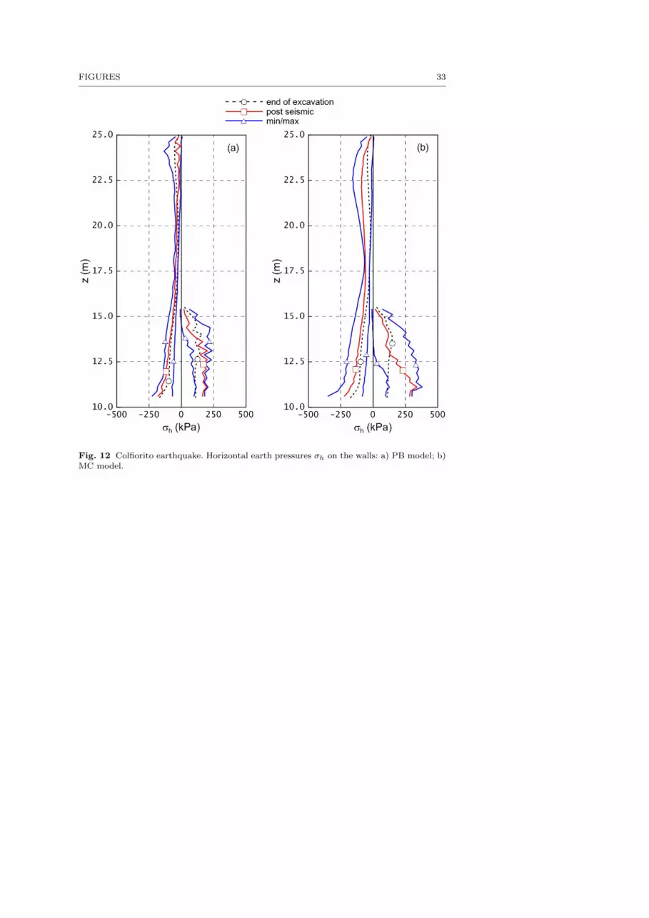
Figs. 12 and 13 show the horizontal earth pressures acting on both sides ofthe left wall, at the end of excavation and in post–seismic conditions. In thefigures, the envelopes of minimum and maximum pressures during the seismicloading stage are also plotted as dashed blue lines. No smoothing procedurehas been applied to the computed stress values at Gauss points.



For the both seismic inputs, the earth pressure distributions obtained withthe two soil models are qualitatively similar. However, smaller peak and post–seismic pressures are predicted by the PB model, particularly for the Colfioritoearthquake.

The observed quantitative difference is reflected in the computed structuralloads, as shown in Figs. 14 to 16. Figs. 14 and 15 show the post–seismic andmin/max envelopes of the bending moments on the left wall for the Colfioritoand Assisi earthquakes, respectively. Fig. 16 plots the evolution with timeof the strut axial load as computed for the PB and MC models for the twodifferent earthquakes.




As expected, both the maximum seismic and post–seismic bending mo-ments computed with the MC model are significantly larger than the corre-sponding values obtained in the simulation with the PB model for both seismicinputs. In particular, the normalized maximum increase in bending momentfrom the initial static conditions (st) to the post–seismic conditions (ps), com-puted as:

∆M = maxz∈[zmin,zmax]

(|Mps −Mst||Mst|

)is equal to +130% for the PB model and +320% for the MC model for theColfiorito earthquake. The corresponding values of ∆M for the Assisi earth-quake are +250% (PB model) and +390% (MC model), respectively.


Similar conclusions apply to the computed strut loads (Fig. 16). For bothseismic inputs, the strut loads computed with the MC model are consistentlylarger than those computed with the PB model, both during the seismic load-ing stage and in post–seismic conditions. In particular, the normalized maxi-mum increase in strut loads from the initial static conditions (st) to the post–seismic conditions (ps), computed as:

∆N =|Nps −Nst||Nst|

is almost zero for the PB model and equal to +140% for the MC model for theColfiorito earthquake. The corresponding values of ∆N for the Assisi earth-quake are +60% (PB model) and +160% (MC model), respectively.

For both earthquakes, the maximum strut load is reached during the earth-quake in the simulations with the PB model, while in the simulations with theMC model the strut load increases almost monotonically with time up to thefinal post–seismic values. Moreover, while N increases gradually and then de-creases during the shake in the PB model simulations, when the MC modelis adopted, N experiences the largest increases in a limited number of spe-cific time increments; this reflects the different ways in which the two modelsdescribe the accumulation of the plastic deformations in the surrounding soil.

In order to better clarify this last point, the shear stress increment ∆τxzvs. shear strain increment ∆γxz curves, obtained with the two models at thetwo points P1 and P2 (see Fig. 1) for the Colfiorito and Assisi earthquakes,are plotted in Figs. 17 and 18, respectively.




From the figure it can be observed that the MC model responds almost elasti-cally during most of the cycles and plastic strains develop only for those largeamplitude cycles capable of bringing the stress state to the local failure condi-tions. On the contrary, given the small size of its yield locus, the PB model iscapable of reproducing more realistically the progressive development of plas-tic strains as the deviatoric stress level increases from geostatic conditions toultimate failure at large strains and to reproduce the hysteresis loops typicallyobserved in coarse–grained soils under cyclic loading conditions.

7 Concluding remarks

The main focus of this work has been to compare the seismic performance ofan idealized – but nonetheless realistic – propped diaphragm wall obtained ina series of dynamic nonlinear FE simulations, performed with two different soilmodels: a classical elastic–perfectly plastic model for cohesive–frictional ma-terials and an advanced anisotropic hardening, critical state model for sands.

This has allowed to gain some insight into the predictive capabilities ofcurrently available design tools – including general purpose FE codes incorpo-rating the MC model in their materials library – when applied to the quantita-tive prediction of the performance (in terms of accumulated displacements ormaximum increments in structural loads) of this particular type of retainingstructures under seismic loading conditions.

The most significant observation obtained from the comparison of the twomodel predictions is that, while under quasi–static, monotonic loading condi-tions (excavation stage) the predicted structural performance is almost insen-sitive to the finer details of the adopted constitutive model – confirming theprevious findings of Burd and Houlsby and Viggiani and Tamagnini [6,38,39]– the same is not true when cyclic/dynamic loading conditions are involved(earthquake loading stage).

In particular, two features of the advanced PB model appear to be mainlyresponsible for the largely different cyclic/dynamic response of the system atthe global level:

a) the limited size of the yield surface, as compared to the large elastic domainof the MC model, and

b) the anisotropic hardening law for the internal variable α, which allows theyield locus to rotate around the origin of the stress space.

These two features of the PB model allow reverse plastic yielding to occureven for relatively small amplitude deviatoric stress cycles, and to obtain anirreversible and hysteretic response of the material whereas the MC modelresponse remains substantially elastic during most of the seismic event. Forthe aforementioned reasons, the situation is not likely to be improved by us-ing more sophisticated isotropic hardening models for the soil – such as, forexample, the Cap Model employed in [34] and [33] – which, although moreperformant than the MC model for monotonic loading conditions, lack boththe aforementioned features.


As expected, the greater ductility in the material response allowed by theadvanced PB model gives rise to computed performances of the retaining struc-tures characterized by larger displacements and smaller structural loads. Thisis consistent with what has been observed by Gazetas et al. [14] in comparingsome FE predictions of gravity and anchored retaining walls obtained withlinear elastic and elastic–perfectly plastic soil models.

As the differences observed in both displacement and load performance in-dicators are substantial, a note of caution is required whenever FE simulationsconducted with currently available perfectly plastic or isotropic hardening soilmodels are employed to evaluate the seismic performance of this type of retain-ing structures in terms of accumulated displacements, or to validate simplifiedperformance–based approaches for their seismic design.

References

1. Alrumoli, K., Muraleetharan, K., Hossain, M., Fruth, L.: Velacs laboratory testing pro-gram – soil data report. Tech. rep., The Earth Technology Corporation, NSF, Wash-ington, D.C. (1992)

2. Alyami, M., Wilkinson, S.M., Rouainia, M., Cai, F.: Simulation of seismic behaviourof gravity quay wall using a generalized plasticity model. In: Proceedings of the 4thinternational conference on earthquake geotechnical engineering, Thessaloniki, Greece(2007)

3. Basha, B.M., Sivakumar Babu, G.: Seismic rotational displacements of gravity walls bypseudodynamic method with curved rupture surface. Int. J. of Geomechanics, ASCE10(3), 93–105 (2010)

4. Been, K., Jefferies, M.G.: A state parameter for sands. Geotechnique 35(2), 99–112(1985)

5. Borja, R.I.: Plasticity: Modeling & Computation. Springer Science & Business (2013)6. Burd, H.J., Houlsby, G.T.: Prediction and performance. In: G.T. Houlsby, A.N. Schofield

(eds.) Predictive Soil Mechanics, pp. 38–49. Thomas Telford, London (1993)7. Callisto, L., Soccodato, F.M.: Performance–based design of embedded retaining walls

subjected to seismic loading. In: Proc. Workshop: Eurocode 8 Perspectives from theItalian Standpoint (2009)

8. Callisto, L., Soccodato, F.M.: Seismic design of flexible cantilevered retaining walls. J.of Geotech. and Geoenv. Engng., ASCE 136(2), 344–354 (2010)

9. Clough, R.W., Penzien, J.: Dynamics of structures, vol. 634. McGraw-Hill New York(1993)

10. Cubrinovski, M., Ishihara, K.: State concept and modified elastoplasticity for sand mod-elling. Soils and Foundations 38(4), 213–225 (1998)

11. Desai, C., Zaman, M., Lightner, J., Siriwardane, H.: Thin-layer element for interfacesand joints. International Journal for Numerical and Analytical Methods in Geomechan-ics 8(1), 19–43 (1984)

12. Elms, D.G., Richards, R.: Seismic design of retaining walls. In: Design and performanceof earth retaining structures, pp. 854–871. ASCE (1990)

13. Gajo, A., Wood, D.M.: A kinematic hardening constitutive model for sands: the multi-axial formulation. Int. J. Num. Anal. Meth. Geomech. 23, 925–965 (1999)

14. Gazetas, G., Psarropoulos, P., Anastasopoulos, I., Gerolymos, N.: Seismic behaviour offlexible retaining systems subjected to short-duration moderately strong excitation. SoilDyn. and Earthquake Engng. 24(7), 537–550 (2004)

15. Gudehus, G., Amorosi, A., Gens, A., Herle, I., Kolymbas, D., Masın, D., Muir Wood, D.,Niemunis, A., Nova, R., Pastor, M., et al.: The soilmodels. info project. Internationaljournal for numerical and analytical methods in geomechanics 32(12), 1571–1572 (2008).URL http://www.soilmodels.info


16. Hibbitt, Karlsson, Sorensen: ABAQUS: Theory Manual. Hibbitt, Karlsson & Sorensen(2002)

17. Iai, S., Ichii, K., Liu, H., Morita, T.: Effective stress analyses of port structures. Soilsand Foundations 38, 97–114 (1998)

18. Ishihara, K., Tatsuoka, F., Yasuda, S.: Undrained deformation and liquefaction of sandunder cyclic stresses. Soils and Foundations 15(1), 29–44 (1975)

19. Kuhlemeyer, R.L., Lysmer, J.: Finite element method accuracy for wave propagationproblems. Journal of Soil Mechanics & Foundations Div 99(Tech Rpt) (1973)

20. Lanzo, G., Pagliaroli, A., D’Elia, B.: Influenza della modellazione di Rayleigh dellosmorzamento viscoso nelle analisi di risposta sismica locale. In: Proc. XI Italian NationalConference: “L’ingegneria Sismica in Italia” (in Italian) (2004)

21. Martinelli, M.: Comportamento dinamico di fondazioni su pali in sabbia (in italian).Ph.D. thesis, Universita degli Studi di Roma La Sapienza (2012)

22. Masın, D., Bohac, J., Tuma, P.: Modelling of a deep excavation in a silty clay. In:Proceedings of the 15th European conference on soil mechanics and geotechnical engi-neering, vol. 3, pp. 1509–1514 (2011)

23. Ministero delle Infrastrutture: Decreto del 14/01/2008 – Norme Tecniche per leCostruzioni. Gazzetta Ufficiale della Repubblica Italiana (in Italian) (2008)

24. Miriano, C.: Modellazione numerica della risposta sismica di strutture di sostegnoflessibili (in italian). Ph.D. thesis, Universita degli Studi di Roma La Sapienza (2011)

25. Mroz, Z., Pietruszczak, S.: A constitutive model for sand and its application to cyclicloading. Int. J. Num. Anal. Meth. Geomech. 7, 305–320 (1983)

26. Newmark, N.M.: Effects of earthquakes on dams and embankments. Geotechnique15(2), 139–160 (1965)

27. Nova, R., Wood, D.M.: A constitutive model for sand in triaxial compression. Interna-tional Journal for Numerical and Analytical Methods in Geomechanics 3(3), 255–278(1979)

28. Papadimitriou, A.G., Bouckovalas, G.D.: Plasticity model for sand under small andlarge cyclic strains: a multiaxial formulation. Soil Dyn. and Earthquake Engng. 22,191–204 (2002)

29. Papadimitriou, A.G., Bouckovalas, G.D., Dafalias, Y.F.: Plasticity model for sand undersmall and large cyclic strains. J. of Geotech. and Geoenv. Engng., ASCE 127(11), 973–983 (2001)

30. Pastor, M., Zienkiewicz, O.C., Leung, K.H.: Simple model for transient soil loading inearthquake analysis. II: non–associative model for sands. Int. J. Num. Anal. Meth.Geomech. 9, 477–498 (1985)

31. Richards, R., Elms, D.G.: Seismic passive resistance of tied-back walls. J. of Geotech.Engng., ASCE 118(7), 996–1011 (1992)

32. Scasserra, G., Lanzo, G., Stewart, J.P., D’Elia, B.: Sisma (site of italian strong motionaccelerograms): a web-database of ground motion recordings for engineering applica-tions. In: AIP Conference Proceedings, vol. 1020, p. 1649 (2008)

33. Siller, T.J., Dolly, M.O.: Design of tied–back walls for seismic loading. J. of Geotech.Engng., ASCE 118(11), 1804–1821 (1992)

34. Siller, T.J., Frawley, D.D.: Seismic response of multianchored retaining walls. J. ofGeotech. Engng., ASCE 118(11), 1787–1803 (1992)

35. Sloan, S.: Substepping schemes for the numerical integration of elastoplastic stress–strain relations. Int. J. Num. Meth. Engng. 24(5), 893–911 (1987)

36. Tamagnini, C., Viggiani, G., Chambon, R., Desrues, J.: Evaluation of different strate-gies for the integration of hypoplastic constitutive equations: Application to the CLoEmodel. Mech. Cohesive–Frictional Materials 5, 263–289 (2000)

37. Van Eekelen, H.A.M.: Isotropic yield surfaces in three dimensions for use in soil me-chanics. International Journal for Numerical and Analytical Methods in Geomechanics4(1), 89–101 (1980)

38. Viggiani, G., Tamagnini, C.: Hypoplasticity for modeling soil non–linearity in excava-tion problems. In: M. Jamiolkowski, R. Lancellotta, D. Lo Presti (eds.) Pre–failureDeformation Characteristics of Geomaterials, pp. 581–588. Balkema, Rotterdam (1999)

39. Viggiani, G., Tamagnini, C.: Ground movements around excavations in granular soils:a few remarks on the influence of the constitutive assumptions on fe predictions. Me-chanics of Cohesive–frictional Materials 5(5), 399–423 (2000)


40. Wang, Z.L., Dafalias, Y.F., Shen, C.K.: Bounding surface hypoplasticity model for sand.J. of Engng. Mechanics, ASCE 116(5), 983–1001 (1990)

41. Whitman, R.V.: Seismic design and behavior of gravity retaining walls. In: Design andperformance of earth retaining structures, pp. 817–842. ASCE (1990)

42. Zeng, X., Steedman, R.: Rotating block method for seismic displacement of gravitywalls. J. of Geotech. and Geoenv. Engng., ASCE 126(8), 709–717 (2000)

43. Zienkiewicz, O.C., Leung, K.H., Pastor, M.: Simple model for transient soil loadingin earthquake analysis. I: basic model and its application. Int. J. Num. Anal. Meth.Geomech. 9, 453–476 (1985)


List of Figures

1 Problem geometry and finite element discretization adopted(only half of the domain is shown). . . . . . . . . . . . . . . . . 22

2 Exemplary pure shear stress-strain (τ -γ) relation according tothe proposed Ramberg-Osgood type shear formulation - effectof a1 (from [28]). . . . . . . . . . . . . . . . . . . . . . . . . . . 23

3 Yield, critical, bounding and dilatancy surfaces of the PB model:a) in q : p plane; b) in deviatoric plane (redrawn from [28]). . . 24

4 Seismic input considered: a) Colfiorito earthquake; b) Assisiearthquake. . . . . . . . . . . . . . . . . . . . . . . . . . . . . . 25

5 Fourier amplitude spectra of the seismic input considered: a)Colfiorito earthquake; b) Assisi earthquake. . . . . . . . . . . . 26

6 Wall displacements at the end of excavation stage. . . . . . . . 277 Wall bending moments at the end of excavation stage. . . . . . 288 Colfiorito earthquake. Horizontal acceleration at point P3 on

ground surface: a) base; b) point P3, MC model; c) point P3,PB model. . . . . . . . . . . . . . . . . . . . . . . . . . . . . . . 29

9 Assisi earthquake. Horizontal acceleration at point P3 on groundsurface: a) base; b) point P3, MC model; c) point P3, PB model. 30

10 Fourier spectra of computed acceleration at point P3: a) Colfior-ito earthquake; b) Assisi earthquake. . . . . . . . . . . . . . . . 31

11 Wall displacements at the end of seismic loading stage. . . . . . 3212 Colfiorito earthquake. Horizontal earth pressures σh on the walls:

a) PB model; b) MC model. . . . . . . . . . . . . . . . . . . . . 3313 Assisi earthquake. Horizontal earth pressures σh on the walls:

a) PB model; b) MC model. . . . . . . . . . . . . . . . . . . . . 3414 Colfiorito earthquake. Bending moments on the left wall: a) end

of excavation and post–seismic values; b) envelopes of minimu-mum and maximum values. . . . . . . . . . . . . . . . . . . . . 35

15 Assisi earthquake. Bending moments on the left wall: a) endof excavation and post–seismic values; b) envelopes of minimu-mum and maximum values. . . . . . . . . . . . . . . . . . . . . 36

16 Time history of strut axial load: a) Colfiorito earthquake; b)Assisi earthquake. . . . . . . . . . . . . . . . . . . . . . . . . . 37

17 Shear stress increment ∆τxz vs. shear strain increment ∆γxzduring the seismic loading stages of Colfiorito earthquake: a)point P1; b) point P2. . . . . . . . . . . . . . . . . . . . . . . . 38

18 Shear stress increment ∆τxz vs. shear strain increment ∆γxzduring the seismic loading stages of Assisi earthquake: a) pointP1; b) point P2. . . . . . . . . . . . . . . . . . . . . . . . . . . 39

22 FIGURES

Fig. 1 Problem geometry and finite element discretization adopted (only half of the domainis shown).

FIGURES 23

Fig. 2 Exemplary pure shear stress-strain (τ -γ) relation according to the proposedRamberg-Osgood type shear formulation - effect of a1 (from [28]).

24 FIGURES

(a)

(b)

Fig. 3 Yield, critical, bounding and dilatancy surfaces of the PB model: a) in q : p plane;b) in deviatoric plane (redrawn from [28]).

FIGURES 25

Fig. 4 Seismic input considered: a) Colfiorito earthquake; b) Assisi earthquake.

26 FIGURES

Fig. 5 Fourier amplitude spectra of the seismic input considered: a) Colfiorito earthquake;b) Assisi earthquake.

FIGURES 27

Fig. 6 Wall displacements at the end of excavation stage.

28 FIGURES

Fig. 7 Wall bending moments at the end of excavation stage.

FIGURES 29

Fig. 8 Colfiorito earthquake. Horizontal acceleration at point P3 on ground surface: a)base; b) point P3, MC model; c) point P3, PB model.

30 FIGURES

Fig. 9 Assisi earthquake. Horizontal acceleration at point P3 on ground surface: a) base;b) point P3, MC model; c) point P3, PB model.

FIGURES 31

Fig. 10 Fourier spectra of computed acceleration at point P3: a) Colfiorito earthquake; b)Assisi earthquake.

32 FIGURES

Fig. 11 Wall displacements at the end of seismic loading stage.

FIGURES 33

Fig. 12 Colfiorito earthquake. Horizontal earth pressures σh on the walls: a) PB model; b)MC model.

34 FIGURES

Fig. 13 Assisi earthquake. Horizontal earth pressures σh on the walls: a) PB model; b) MCmodel.

FIGURES 35

Fig. 14 Colfiorito earthquake. Bending moments on the left wall: a) end of excavation andpost–seismic values; b) envelopes of minimumum and maximum values.

36 FIGURES

Fig. 15 Assisi earthquake. Bending moments on the left wall: a) end of excavation andpost–seismic values; b) envelopes of minimumum and maximum values.

FIGURES 37

Fig. 16 Time history of strut axial load: a) Colfiorito earthquake; b) Assisi earthquake.

38 FIGURES

Fig. 17 Shear stress increment ∆τxz vs. shear strain increment ∆γxz during the seismicloading stages of Colfiorito earthquake: a) point P1; b) point P2.

FIGURES 39

Fig. 18 Shear stress increment ∆τxz vs. shear strain increment ∆γxz during the seismicloading stages of Assisi earthquake: a) point P1; b) point P2.

40 FIGURES

List of Tables

1 PB model constants for Nevada Sand (from [28]). . . . . . . . . 412 MC model constants for Nevada Sand. . . . . . . . . . . . . . . 423 Rayleigh damping parameters assumed in the simulations with

the MC model. . . . . . . . . . . . . . . . . . . . . . . . . . . . 434 Geometry and material constants for r.c. structural elements. . 445 Characteristic parameters of the seismic inputs considered. . . 456 Program of FE simulations. . . . . . . . . . . . . . . . . . . . . 46

TABLES 41

Γ λ Mcc Mc

e m B a1 γ1

0.809 0.022 1.25 0.90 0.0625 520 0.67 2.5e-4

ν kbc kdc A0 h0 H0 ζ C

0.31 1.45 0.3 2.1 5.0e3 6.8e4 1.0 130

Table 1 PB model constants for Nevada Sand (from [28]).

42 TABLES

G ν c φ ψ

(kPa) (–) (kPa) (deg) (deg)

variable 0.31 0.0 32 15

Table 2 MC model constants for Nevada Sand.

TABLES 43

Seismic input ω1 ωIN n ωn αR βR

(rad/s) (rad/s) (–) (rad/s) (–) (–)

Colfiorito WE 16.33 78.54 5 81.65 1.36 1.02e-3

Assisi NS 16.33 19.63 3 48.99 1.22 1.53e-3

Table 3 Rayleigh damping parameters assumed in the simulations with the MC model.

44 TABLES

t E ν γ

(m) (kPa) (–) (kPa)

1.0 2.0e7 0.25 25.0

Table 4 Geometry and material constants for r.c. structural elements.

TABLES 45

Earthquake amax T f d IA

(g) (s) (Hz) (s) (m/s)

Colfiorito WE 0.2 0.08 12.50 11.40 0.322

Assisi NS 0.2 0.32 3.13 4.14 0.264

Table 5 Characteristic parameters of the seismic inputs considered.

46 TABLES

Run Seismic Constitutive C

# input model (–)

C–01 Colfiorito WE PB 130

C–02 Colfiorito WE MC –

A–01 Assisi NS PB 130

A–02 Assisi NS MC –

Table 6 Program of FE simulations.

Documents

Advanced numerical modeling of seismic response of a propped r.c. diaphragm wall