Additive structure in qualitative data: An alternating least squares method with optimal scaling features

PSYCHOMETRIKA--VOL. 41, NO. 4

DECEMBER, 1976

ADDITIVE STRUCTURE IN QUALITATIVE DATA:AN ALTERNATING LEAST SQUARES METHOD

WITH OPTIMAL SCALING FEATURES

JAN DE LEEUW

RIJKSUNIVERSITEIT TE LEIDEN

FORREST W. YOUNG AND YOSH~O TAKANE

UNIVERSITY OF NORTH CAROLINA

A method is developed to investigate the additive structure of data that(a) may be measured at the nominal, ordinal or cardinal levels, (b) may be tained from either a discrete or continuous source, (c) may have knowndegrees of imprecision, or (d) may be obtained in unbalanced designs. Themethod also permits experimental variables to be measured at the ordinal level.It is shown that the method is convergent, and includes several previouslyproposed methods as special cases. Both Monte Carlo and empirical evalua-tions indicate that the method is robust.

Key words: linear model, analysis of variance, measurement, successive blockalgorithm, quantification, data analysis.

In this paper we consider ways to obtain ~dditive representations ofdata structures. This problem is not new, of course; it has ~ long historyunder the misnomer "analysis of variance". We are not so presumptuousas to consider all aspects of the problem. Rather, we focus our efforts on a

particularly robust way to obtain additive representations for qualitative

data structures, i.e., those with nominal and/or ordinal data.Even this problem is not new. As early as 1938, Fisher [1938, pp. 285-298]

proposed an eigenvector method for applying the simple additive model to

nominal data, a method which has been rediscovered periodically over theyears [Hayashi, 1952; Carroll, Note 2; Nishisato, Note 7, Note 8]. Morerecently Kruskal [1965] proposed a gradient procedure for investigating

the additive structure of ordinal data [see also Roskam, 1968; de Leeuw,Note 3; Lingoes, 1973]. Our work is strongly related to de Leeuw’s [1973]

This research was supported in part by grant MH-10006 from the National Instituteof Mental Health to the Psychometric Laboratory of the University of North Carolina.We wish to thank Thomas S. Wallsten for comments on an earlier draft of this paper.Copies of the paper and of ADDALS, a program to perform the analyses discussed herein,may be obtained from the second author.

Requests for reprints should be sent to Forrest W. Young, Psychometric Laboratory,University of North Carolina, Davie Hall 013 A, Chapel Hill, North Carolina 2571.4.

471

472 PSYCItOMETRIKA

discussion of methods for analyzing nominal data and to Young’s [1972]alternating least squares method for finding additive structure in ordinal data.

Our work is placed in a theoretical framework from which flows anelegant and simple method for investigating additive structure in qualitativedata, including as special cases all the methods mentioned in the precedingparagraph. The data may be defined at the nominal, ordinal or interval levelsof measurement, or may be a mixture of two or three levels. In any case theobservation categories may represent an underlying process which is eitherdiscrete or continuous, an important theoretical and practical distinctionwhich is seldomly discussed in this context. It is also very simple, within ourframework, to introduce constraints on the parameters of the additive model.Thus, for example, it is quite simple to specify ordinal constraints for somefactor in a design, if there is a priori reason to do so. Finally, our frameworkallows us to investigate observations arising in certain unbalanced, incom-plete factorial designs. If, for example, we have a replicated factorial design,but have been unable to obtain an equal number of observations in all cellsof the design, our developments can still be applied.

1. Introduction

The analysis of additivity has usually been introduced in the contextof a statistical model for factorially classified observations, requiring assump-tions that are often very strong and unrealistic. In many situations muchless specific models are called for, based on much weaker assumptions. Wediscuss the classical assumptions briefly.

In stochastic versions of the analysis of additivity, one analyzes a model(Model S) whose assumptions are

S~: Y~i = ~’+a~ +~i +S~ : the e, are independent random variables,S~ : the e, have a eentered normal distribution with finite variance ~.

(A bold face symbol is used to distinguish random variables from fixed con-stants). Model S generalizes in a straightforward way to ineomplete and/orreplicated multi-factor situations, in which the number of indices and ofcorresponding sets of parameters is larger. (In order to avoid eumbersomenotation we shall only treat the two-factor ease in this paper. The generali-zations to more eompfieated factorial designs are obvious.)

Observe that S does not say that there are parameters % a~ , ~ suchthat each additive combination ~, + a~ + B; is close to the correspondingy, ; it merely makes a statement about the two-way strueture of the expeeta-tions E(y,). The variance e can be arbitrarily large, and if it is unknown(which is the usual ease), we can only test hypotheses abou~ the parameterswithin S (i.e., while assuming S to be true). In many eases S itself is not veryreasonable, as the parametric assumption Sa is too strong in many applica-tions. Even the independence assumption S~ is often not obviously true.

JAN DE LEEUW, FORREST W. YOUNG AND YOSH[O TAKANE 473

Within the framework of established statistical theory, the logical stepout of these difficulties would seem to be to make weaker, nonparametricassumptions. Model N, a straightforward extension of S, involves the fol-lowing nonparametric assumptions:

N~: y~; = ~,+a~+~i+~i,N2 : the ~ are independent random variables,N~ : the ~ have a centered, centrally symmetric, continuous distribution

~vith finite variance.Unfortunately, the statistical theory based on the assumptions of this modelis fragmentary, and from the point of view of data analysis, inferior to thatbased on Model S.

In the case of Model S, the natural estimation method and the optimalway of testing hypotheses follow directly from elementary properties of themodel. The method of least squares should be used. The orthogonality prop-erties of the complete factorial design lead to additive partitionings of the sumsof squares and to optimal tests of hypotheses. These properties are veryvaluuble for summarizing some of the important structures in the data.Model N, on the other hand, leads to robust significance testing and estima-tion, but the properties of the tests and estimates are usually only approxi-mately known, and the beautiful structure of a complete least-squaresanalysis is lost. Refer to Purl and Sen [1971] for a summary of some of theresults that can be obtained.

Another basic complication is that in many applications even the assump-tion S~ or N1 cannot be applied because the observed data are qualitative.That is, they consist of a small number of categories for which no precisenumerical values are known. This not only violates the assumption of acontinuous distribution, but it also makes $1 and N, meaningless becausey~ is not defined. In this paper we reformulate the basic structural assumptionS~ or N~ in such a way that it also applies to categorical data. For this purposewe use the notion of optimal scaling [Fisher, 1938; Guttman, 1941; Burr, 1950;Bock, Note 1; Nishisato, Note 7; de Leeuw, 1973]. We shall assume thatthe data are in K mutually exclusive and exhaustive categories. We definethe K-ary random variables z~k to be equal to one if the observation in cell(i, ~) of the design is in category 1¢, and equal to zero otherwise. In this simplecase, the model we employ is

K

D~ : ~Z~kOk = ~, + a, + [3~ + ~ii ¯

Observe that we have introduced the optimal sealing parameters O~ , whichwe use to quantify each of the k categories. I~ is through restrietions on theoptimal scaling parameters O~ that ~ve can treat qualitative (as well as quanti-tative) data. If we do not know precise numerie~l values for the observationswe can represent each unique observation by a parameter Ok and try to

474 PSYCHOMETRIKA

parametrize the data (as well as the model) to optimize the fit between thetwo. (Naturally, there must be fewer categories than observations, or wewill have a perfect, but trivial fit.) Since we wish to work in the familiarleast-squares framework, we measure the fit of a particular arbitrary choiceof parameters by a suitably normalized version of the loss function

The comput.ational problem is to choose the parameters 0~ , % al , and ~in such a way that h is minimized.

In the several cases we will discuss, not all vectors of real numbers areadmissible as parameter vectors: i.e., the admissible values for 0~ , a~ , B~ ,and ~ may be subject to certain restrictions. Through these restrictions wecope with a variety of measurement levels. For example, if the data aremeasured at the ordinal level, then we restrict the value of 0~ < 0~: if we knowthat the corresponding dat~ categories stand in this relation. As anotherexample, if we know a priori that the levels of som~ factor (say factor I)have ordinal properties, then we can restrict the estimate of a~ < a~, if thatis the desired order. Other types of useful parameter restrictions will bediscussed in the body of the paper, but we should always keep in mind thatour goal is to optimize, within the least-squares framework, the relationshipbetween a possibly restricted set of model parameters a~ , fl~ , and ~ and apossibly restricted set of optimal scaling parameters ~ .

An important difference between this approach and the one based oneither models S or N is that we have no guarantee that our e.stimates willbe "good" estimates according to any of the accepted statistical criteria.We merely compute estimates, and afterwards we can try to find out howthey behave under various more-or-less specific assumptions about the distri-bution of the z~~. Rather than estimate the parameters of a model in theusual sense, we study the properties of a particular transformation or reduc-tion of the data [cf. also de Leeuw, 1973, Chapter I, for more extensiondiscussion of the difference between the two approaches].

We use a computational method for optimizing h which we call additivityanalysis by alternating least squares (ADDALS). This is an iterative methodwhich alternates between a) minimizing h over all ~dmissible optimal scalingparameters 0~ for fixed values of the model parameters a~ , B~ , and % and b)minimizing h over all admissible model parameters for fixed values of theoptimal scaling parameters. In each of the two phases of an interation theoptimization is complete; that is, the values obtained for one of the sets ofparameters absolutely minimize the function h conditional on a fixed set ofparameters. Thus, the name alternating least squares: we alternate betweentwo phases, one of which determines the (conditionM) least squares estimatesfor the optimal scaling parameters and the other of which determines the(conditional) least squares estimates for the model parameters. This type

JAN DE LEEUW, FORREST W. YOUNG AND YOSttIO TAKANE 475

of procedure is philosophically much like the NILES/NIPALS pr6ceduresdeveloped by Wold and his associates [Wold & Lyttkens, 1969] with thedistinction that Wold is usually concerned with optimizing only model param-eters. The class of procedures used by Wold and by us is known in the mathe-matical programming literature as block relaxation or nonlinear Gauss-Seidel methods. Although our procedure always converges to a stationarypoint it may not be the most robust one for each of the special situationsoutlined above. Thus, we compare our method with others which have beensuggested for some of the special cases, with generally satisfactory results.As will be seen, the iterates are very simple (yielding an algi)rithm whichmay be used on small machines) and very quick (enabling the analysis large problems on large machines).

2. Data Tt~eory

In this section we outline the data theory in which the developmentsof this paper are embedded. This section is divided into three subsections,concerned with the empirical, model, and measurement aspects of the datatheory.

Empirical Aspects

For the sake of simplicity and clarity, we restrict our formal develop-ments to the case where there are only two conditions (called factors, inde-pendent variables, components, dimensions, facets, classifications, etc.,by others). The first condition has n levels (values, elements, structs); second, m levels. We shall assume that each combination of levels (cell,structuple) is replicated R times, an assumption which will be relaxed shortly.Finally, we view the experimental design as being the Cartesian product ofall the conditions and the replication factor.

An assumption fundamental to our work is that an observation is adiscrete entity which belongs to a particular observation category. Specifically,an observation is said to be in the same category as another observation ifthey are indistinguishable from each other in terms of their observationalcharacteristics other than the time and place of observation. Note that thecategories are mutually exclusive and exhaustive subsets of the entire set ofobservations. There are K observation categories in total.

This view of the basic nature of the data allows us to recode the datain a binary form indicating the category membership of each observation.The resulting binary matrix, called the indicator matrix, has one columnfor each observation and one row for each level of each experimental condi-tion, as well as one row for each observation category. Thus, in our situationthere are Rnm columns, and n W m + K rows. The rows of the matrix arepartitioned into three subsets, as follows. The first set of n rows indicatesthe level of the first experimental condition; the second set of m rows indicatesthe level of the second experimental condition; and the last set of K rows

476 PSYCHO.~’IETRIKA

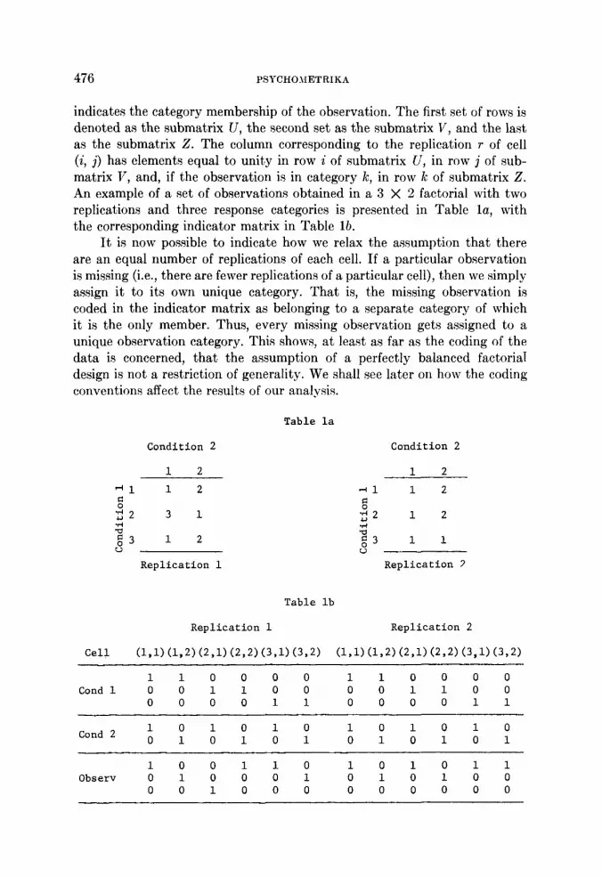
indicates the category membership of the observation. The first set of rows isdenoted as the submatrix U, the second set as the submatrix V, and the lastas the submatrix Z. The column corresponding to the replication r of cell(i, j) has elements equal to unity in row i of submatrix U, in row j of sub-matrix V, and, if the observation is in category ]~, in row ]c of submatrix Z.An example of a set of observations obtained in a 3 X 2 factorial with tworeplications and three response categories is presented in Table la, withthe corresponding indicator matrix in Table lb.

It is now possible to indicate how we relax the assumption that thereare an equal number of replications of each cell. If a particular observationis missing (i.e., there are fewer replications of a particular cell), then we simplyassign it to its own unique category. That is, the missing observation iscoded in the indicator matrix as belonging to a separate category of whichit is the only member. Thus, every missing observation gets assigned to aunique observation category. This shows, at least as far as the coding of thedata is concerned, that the assumption of a perfectly balanced factoria!design is not a restriction of generality. We shall see later on how the codingconventions affect the results of our analysis.

~able la

Condition 2 Condition 2

i 2 i 2

~i 1 2 ~i i 2

o o~2 3 1 "~2 1 2

o=3 1 2 o=3

Replication 1 Replication P

Table ib

Replication i Replication 2

Cell (i,i) (i, 2) (2,1) (2,2) (3,I) (3,2) (1,1)(1,2)(2,1)(2,2)(3,1)(3,2)

1 i 0 0 0 0 i i 0 0 0 0Cond i 0 0 1 1 0 0 0 0 1 i 0 0

0 0 0 0 1 i 0 0 0 0 1 1

1 0 i 0 1 0 i 0 i 0 1 0Cond 2

0 1 0 i 0 1 0 1 0 i 0 i

i 0 0 1 i 0 i 0 i 0 i iObserv 0 1 0 0 0 1 0 1 0 1 0 0

0 0 1 0 0 0 0 0 0 0 0 0

JAN DE LEEUW, FORREST W. YOUNG AND YOSHIO TAKANE 477

Model Aspects

The model involves concepts which parallel those involved in theempirical situation. Corresponding to the two experimental conditions aretwo vectors of parameters. Just as each condition has levels, each parametervector has elements, denoted al and ~; (we use Greek characters for param-eters). There is no notion in the model which corresponds to the empiricalnotion of replications, since we assume that any differences which arise be-tween replications are random fluctuations not included in the model. (Ifwe were in fact interested in modeling these fluctuations, then we wouldview the "replications" factor as an additional experimental condition.)Finally, there is a direct correspondence between the experimental designand the model. Whereas the former involves the Cartesian product of all theexperimental conditions and the replication factor, the latter involves thefactorial combination of all the parameter vectors. For both the Cartesianproduct and the factorial combination we define two real-valued functionswhich generate the data and model spaces, respectively. Thus, the modelspace is defined by

b:cli = ~,+~i,

and the data space byK

t: y,.i = ~_, zi~kO~ .

In matrix notation these definitions are

1: C = Us-t- V~,

t: Y = ZO.

Finally, as mentioned above, we wish to parameterize the two spacesso that they are as much alike as possible. This objective is realized in theusual way of minimizing the sum of squared error terms. Thus, we wish tominimize (subject to normalization)

or in matrix terminology

X = trace (ZO - Ua - V~)’(ZO - Ua - V~),

by judicious assignment of values to the parameters of the two spaces. Theminimization is subject to constraints which we may place on the parameters.These constraints are discussed in the next section.

Measurement Aspects

In this section we discuss those restrictions that may be placed on thedata and model parameters. It is through these restrictions that we are able

478 PSYCHO.~tETRIKA

to treat the variety of measurement conditions under which the observationsmay have been obtained, including the level and precision of measurement,the nature of the process which may have generated the observation, and themeasurement characteristics of the experimental conditions themselves.We distinguish three types of parameter restrictions, identification restric-tions, model restrictions, and data restrictions, and discuss them in turn.

Identification restrictions. Note that the model

c,~ = ai+~i,

can be written as

with a~ and ~i restricted in such a way that

i=1

These constraints merely serve to identify the model parameters, since with-out them we can add a constant to all a~ and subtract the same constantfrom all ~i without affecting the fit. We shall always impose these constraints,but they must be distinguished from other types of constraints which gobeyond the basic specifications of the model and data spaces.

Model restrictions. There are two .types of optional restrictions whichmay be placed on the permissible values of a, and f~i and may be appropriatein certain situations. One type of restriction is invoked when we know thatthe levels of one (or both) of the experimental conditions fall in some a prioriorder. In such a situation we restrict the corresponding model parameters(a~ or Bi) to be in the desired order. The other type of restriction applieswhen we know that the levels of an experimental condition are related toeach other in some clearly specified functional manner, for example bylinear or polynomial function. In this situation the parameter vector isrestricted to be a function of a fixed and known vector.

Data restrictions. The restrictions on the optimal scaling parameters0~ are somewhat more complex than those just presented. These restrictionsfall into two classes which are factorially combined to produce six types ofdata which differ in terms of their measurement characteristics.

The first class of restrictions is concerned with the measurement levelof the data, and is precisely the same as that discussed in the previous section.That is, there are order restrictions on ~ when the data are ordinal, and linear(or other functional) restrictions on 0~ when the data are numerical. Just the model parameters, the data parameters may also be unrestricted which,when combined with the process restrictions discussed in the next paragraph,implies that the observations are measured at the nominal level.

The second class of restrictions on the optimal scaling parameters


corresponds to our assumptions about the process which generated the obser-vations. If we believe that the process is discrete, then we restrict all theobservations in a particular category to be represented by a single, discretenumber. Thus in this case the optimal scaling parameter ~k is a single numberfor each It. On the other hand, if we believe that the process is continuous,then we define 0k to be a bounded interval of numbers so that all the observa-tions in a particular category are represented by a number in the interval.

By factorially combining the three level restrictions (no restrictions,order restrictions, and numerical restrictions) with the two process restrictions(discrete and continuous), we obtain six types of restrictions on the parameter-ization of 0k , which correspond to six different types of measurement, asfollows. When we combine the "no" level restrictions with either one of thetwo process restrictions, we obtain two different forms of what are commonlycalled nominal data. The discrete process restrictions are appropriate to datadefined at the nominal level. In this case all observations in a given categoryare assigned a single number, with no restrictions between the variouscategories. We call this well-known case the discrete-nominal case. Onthe other hand, when the process is assumed to be continuous, we obtainpermissible parameterizations of ~ which are appropriate to what we callcontinuous-nominal data. Here we assign a range of numbers of observationsin each category, with no restrictions between categories. Obviously, therequirement that all observations in a category must be quantified by aninterval is much too weak, as any arbitrary quantification always satisfiesthe restrictions if the category intervals are wide enough. Thus, we needto specify additional restraints. One possibility for achieving meaningfuland non-trivial boundaries is to view the supposedly continuous-nominal dataas actually being continuous-ordinal (to be discussed in a moment), but withthe order of the categories unknown. We call this the pseudo-continuous-ordinal case.

When we combine the ordinal restrictions with either of the processrestrictions, we obtain the two commonly discussed forms of ordinal datathat correspond to how tied observations are handled. The discrete-ordinalcombination is appropriate ~vhen tied observations are to remain tied.(Kruskal, 1964, calls this the secondary approach to ties.) The continuous-ordinal combination is used when tied observations are to be untied. (Kruskalcalls this the primary approach to ties.)

When we combine the numerical restrictions with either of the processrestrictions, we obtain a measurement level which corresponds to two formsof numerical (quantitative, cardinal) data. What is most commonly thoughtof as numerical data is obtained when the discrete process restriction is used,since in this case all observations which are equal (i.e., in the same category)remain equal (are parameterized by a single 0k) and all observations whichare not equal (in different categories) are functionally related. On the other

PSYCHOMETRIKA

hand, when we use the continuous process, we obtain a form of numericaldata whose measurement characteristics take into consideration the precisionof measurement, since in this case each observation is functionally relatedto every other observation within a certain degree of tolerance. The degreeis specified by the width of the interval around each observation. Note that

¯ there is a subtle difference between the present usage of interval restrictionsand the previous usage. Whereas previously we assumed that the boundariesof the intervals were determined internally (i.e., according to the natureof the data and model), we now assume that the boundaries are specifiedexternally before the data are analyzed. Thus we assume that the researchercan specify an upper boundary ~k÷ and a lower boundary ~k- on each observa-tion category. Generally, there is but one observation in each category fornumeric data, so we are usually specifying a precision interval for every singleobservation. In many situations we will wish to specify an interval of constantwidth for all observations, with the midpoint of the interval being equal tothe observation. That is, we need only to specify Oa from which we candetermine 0k+ = 0k + 0a and 0k- = 0k - Oa. There are other interestinguses of the continuous-numerical parameter restrictions. For example, externalboundary constraints can be used to impose nonnegativity (by setting 0k- = and 0k+ = ¢o) or other types of range restraints. External boundary con-straints can also be used to impose constancy on certain portions of the databy setting 0k- = ~k+ = Pk, where pk is a known constant.

3. Method

In this section we present the alternating least squares (ALS) methodthat obtains estimates of the optimal scaling parameters 0k and the additivemodel parameters a~ and $¢ that optimize ~. In the first subsection we discussthe decompositions of the function ~, from which flow the ALS procedureas applied to the additive model (the ADDALS algorithm). In the nextsubsection we discuss parameter restrictions and their least squares imple-mentation in ADDALS. In the third we outline the ADDALS algorithmfor finding the jointly optimal (restricted) parameterization of the modeland data spaces, and prove the convergence of the algorithm under all butthe pseudo-ordinal restrictions. In the fourth section we show that a) theADDALS algorithm is equivalent to the analytic method proposed inde-pendently by Fisher [1938], Hayashi [1952], Carroll [Note 2] and Nishisato[Note 7] for discrete-nominal data; b) the ADDALS algorithm is essentiallyequivalent to the MONANOVA algorithm proposed by Kruskal [1965] forordinal data (discrete or continuous); c) the ADDALS algorithm is equivalentto the widely used ANOVA methods for analyzing discrete-numerical data;and d) the ADDALS algorithm is equivalent to the widely used procedureproposed by Yates [1933] to solve for the optimal values of missing discrete-numerical data. Finally, it is observed that ADDALS obtains least squares


parameter estimates in a wide range of other situations for which, to theauthors’ knowledge, least squares methods have not been previously proposed.

Decompositions

We now introduce the index r for replications explicitly into our equa-tions, by defining the quantified observations as

K

~Y~i ~- Z ~Z~i t~ rOk ~

in the unpartitioned case, or

K(r)

rYli = E rZi/: ~0~ ,

in the partitioned case. (The number of categories need not be the same foreach replication.) From the familiar theory of the analysis of variance wedecompose ,Y~i into orthogonal components, using dots to indicate indicesover which we have averaged. The decomposition we use is

~y, = .y.. + (.y,. -.y..) + (.y.~ -.y..)

+ (.Y,~ -- .y,. -- .y.~ + .Y..) + (~Y,, --.y,).

We then define

~ = .y~. -.y..,

~i = .Y.~ -- .Y.. ,

~ = .y,.~ -- .y~. -- .y.~ + .Y.. ,

Observe ~ha~ ull ~hese quan~i~ies depend on ~he O~ , bu~ ~ha~ we suppress~his dependence ~o keep ghe notation simple.

I~ is well known ~ha~ £, ~ , ~ ~re le~s~ squares estimates of ~he corre-sponding p~rame~ers in ~he model

i.e., they minimize ~he sum of squ~res of ~he residuals ,&i ¯ The correspondingminimum residuals ~re, of course, precisely ,~i ¯ In ~he same way £, & , ~i ,

and % ~ ~re ~he leas~ estimates in ~he model

~nd ,~, is ~he corresponding minimum residual. Although we ~re re’ally

4,~2 PSYCHOMETRIKA

only interested in the first model (any departure from simple additivity isassumed to be error), it is sometimes informative to decompose the residualinto a systematic interaction and error term.

In ordinary analysis of variance, the decomposition of ry~i into orthogo-nal components defines an additive decomposition of the sum of squaresof t.he ,.Yii into components, each of which is the sum of squares of one com-ponent of the ,y,i . In this paper we use the same orthogonality propertiesto partition our loss functions,

into loss function components corresponding to each subset of the parameters.The relevant partition is given in Table 2.

In t~e case in which the purumeters ~re not restricted in uny sense,minimization can obviously be accomplished by minimizing each of thecomponents over the relevant subset of the parameters. This makes eachof the three deviation components equal to zero because we set ~ = ~, a~ = &,and ~ = ~. In the constrained case a similar result is true if the constraintson the parameters are separated (i.e., there are constraints on a, constraintson B, and no constraints that involve both a and B). Thus, the overall mini-mization problem separates into a number of simpler minimization sub-problems. As mentioned previously, we are only interested in the additivemodel in this paper, and the decomposition of the ~$,.¢ into an interaction

Table 2

deviation from optimal mean Rnm

n ^deviation from optimal row Rm ~ (~i-~i)scores i=l

m

deviation from optimal col- Rn

umn scores j 1

SUBTOTAL: deviation fromoptimal parameterization

optimal minimum loss

r=l i=l j=l ¯

R

~ ~ E (r6ij)r=l i=l j=l

total loss for given paramerterization

R n m

~ E ~ (rYij-~-~i- 6j r=l i=l j=l


term "~i and an error.term ,e,i is not really relevant. It is obvious, however,that Table 2 can be modified very easily to include the interaction param-eters. In Young, de Leeuw and Takane [1976] we have done this, and havediscussed restrictions on the interactions in a form which has recently beenstudied extensively in the statistical literature [for example, Corsten & vanEynsberger, 1972].

To derive the second decomposition of our loss function we define

and (in the unpartitioned case)

~vith

Mk = ~-’~ ~ ~"~rz~~,

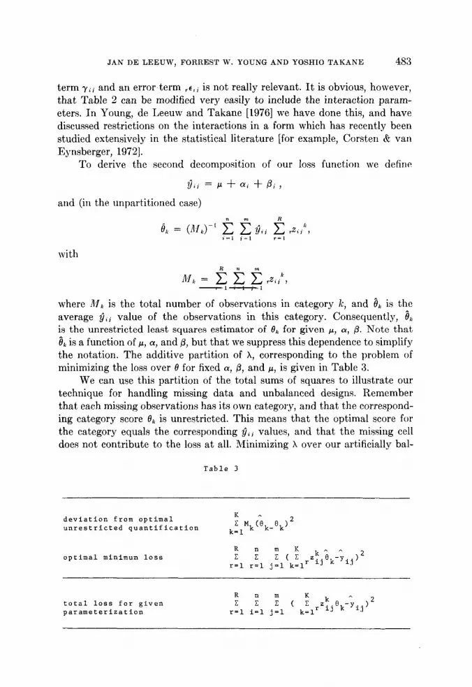
where ~lIk is the total number of observations in category k, and ~ is theaverage 9~ value of the observations in this category. Consequently, 0kis the unrestricted least squares estimator of 0k for given ~, a, ~. Note that0k is a function of u, a, and ~, but that we suppress this dependence to simplifythe notation. The additive partition of X, corresponding to the problem ofminimizing the loss over 0 for fixed a,/3, and ~, is given in Table 3.

We can use this partition of the total sums of squares to illustrate ourtechnique for handling missing data and unbalanced designs. Rememberthat each missing observations has its own category, and that the correspond-ing category score 0~o is unrestricted. This means that the optimal score forthe category equals the corresponding 9~ values, and that the missing celldoes not contribute to the loss at all. Minimizing X over our artificially hal-

Table 3

deviation from optimalK ^E Mk(8 k Ok)2

unrestricted quantificationk=l

optimal minimum lossR n m K k^ ^ )2

rE=l rE=l jE=l(kElrzij~k-Yij=

total loss for givenparameterization

^R n m K k)2E E E ( E z..

r=l i=l j=l k=l r x38k-YiJ

4S4 PSYCHO.~IETRIKA

anced design is equivalent to minimizing a loss function that is the sum ofsquares of the deviations of data and model values in non-missing cells only.This is true for obtaining either 0k or ai and/3i .

Use o] Restrictions

In this section we discuss the implementation of the most importanttypes of restrictions on the parameters in the two computational subproblems(minimizing h for fixed ~ over a,/~, ~, and minimizing h for fixed a, ~, ~ over ~).

For the first problem we may know, a priori, an appropriate order forthe levels of I or J, and therefore may desire to restri’ct the parameters, forexample, sothata~ ~ a~ ~ ... ~ a,,, and/or~ g ~ ~ ... ~ ~ .... Ourfirst decomposition (T~ble 1) shows that the optimal a under these restric-tions can be found by applying the familiar isotonic regression methods[B~rlow, et. al., 1972; Barlow & Brunk, 1972]. Actually, general partial orderson the a~ or the ~ could be incorporated in this way, but the followingdevelopments only cover the linearly ordered case, with Kruskal’s [1964]two methods for incorporating ties. Although our developments are limitedto ordinal restrictions on the model parameters, we could restrict the a~and ~ in other ways. For example, the a~ (or B~) could be required to related by the linear function

~ = a ~ b~+~,

or by some other polynomial function. In such a case the decomposition showsthat ordinary linear regression can be used to compute the least squaresestimates of the linearly related a~ and B~ ̄ (See Young, de Leeuw & Takane,1976, for development of this notion.)

From the second decomposition (Table 3) it follows that explicit intervalrestrictions of the form 0~- ~ 0~ ~ 0~+ with known 0~+ and 0~- (e.g., con-tinuous-numerical data) can be handled very easily. If 9~ is in the interval,then the optimal 0~ is equal to ~. If 9~ is outside the interval, then the optimal0~ is equal to the nearest endpoint of the interval (e.g., equal to 0~+ if ~ > 0~+

or equal to 0~- if 9~ < 0~-). Order restrictions on 0~ can be handled by mono-tone or linear regression again. Using the primary or secondary approachto ties takes care of continuous or discrete ordinal data and discrete categoricaldata. In this last case we set the optimal 0~ equal to ~ .

Only continuous-nominal data present a problem. In the pseudo-ordinalcase we want the optimal 0~ to fall into disjoint intervals, but the order of theintervals on the real line is unknown. Obviously the best procedure is ~o tryout all possible orders of interwls, compute the optimal 0~ by monotoneregression with the primary approach for each interval order, and keep thebest order to define the optimal 0~ for this iteration. This c~n lead to ratherunpleasant computations if the number of categories is at all large, and itintroduces severe discontinuities in our transformation, which affect the


convergence behavior of our algorithm. A second alternative (which is usedin ADDALS) is to derive the optimal order of the intervals from the orderof the ~ . This yields a satisfactory approximation in most cases. Again,discontinuities may present a problem and convergence is not assured, butwe can fix the order of the intervals at the current optimum in the finaliterations, and treat the data as continuous-ordinal in the remaining cycles.This guarantees convergence.

Convergence

In the previous section we showed that each of the two subproblemscan be solved in a very elementary way. Of course, this still does not proveanything about the efficiency or convergence of the complete process ofalternating the two subproblems.

Let us formalize this process somewhat. Assume that there is a pointx in a Euclidian space. Also assume that there is a closed convex subset Cof the same Euclidian space. We define y as the nearest point to x when xis projected onto the subset C, if y uniquely minimizes the Euclidean distancebetween x and y (i.e., minimizes I Ix - YI! where the double bars indicatesums of squares). We denote the nearest point notion as y = C(x), which isread "y is the nearest point projection of the point x onto the closed convexsubset C". Now suppose that there are two closed convex sets C1 and C~ .Our iterative procedure can be viewed, formally, as a process that startswith lc = 0, and with some arbitrary yl0 . The first subproblem proceeds byobtaining C~(y~) (the nearest point in C~ to y~) and setting x~.. C~(y~).The second subproblem goes on to obtain C~(x~) (the nearest point in C.~ to x~0)and then sets y~.÷~ = C,~(x~). The next iteration ensues by incrementing lcand repeating the process.

It is important to understand that we can view our algorithm as in-volving a cyclically repeated series of optimal conic projections because whenwe view it in this light we can prove the convergence of the algorithm. Inorder to see that our algorithm does in fact consist of a series of optimalconic projections, it is necessary to understand that a) ordinal restrictionsforce the parameters to fall in a known convex cone; b) the functional restric-tions we discussed for numerical data form a parameter vector in ap-dimensional subspace, which is a particular type of convex cone; c) con-tinuous process restrictions are restrictions on the parameters to fall in abounded interval, which is a specific type of cone; and that d) discrete ~)rocessrestrictions are also interval restrictions where the interval has zero width(i.e., is a point), which is also a type of cone.

Convergence of a cyclically repeated series of optimal projections canbe proven by theorems already available in’ the literature. First, there aretheorems dealing explicitly with cyclic projection on a finite sequence ofconvex sets. The most general results have been given by Gubin, Polyak, and

4S6 PSYCHOMETRIKA

Raik [1967]. Second, there are some general theorems dealing with theconvergence of block relaxation of convex functions. A representative referenceis C~a and Glowinski [1973]. A useful convergence theorem for nonconvex func-

tions (with stati~.tical applications) is given by Oberhofer and Kmenta [1974].Finally there are a number of general convergence theorems for relaxationprocesses, of which the most familiar one is given by Zangwill [1969]. Itfollows from these theorems that the sequence x, converges, in an infinitenumber of iterations, to a fixed point x= which is the point in C~ which isnearest C~. Moreover, y~ converges to a fixed point y~ which is the point inC2 nearest C~. Consequently, the distance between x~ and y~ is the minimumof all possible distances between x in Cj and y in C2 ̄

These results can be applied directly to the case in which there areinterval restrictions on the O~ , and some restrictions on the a~ and ~ . If-both ~, and a~ , B~ are restricted by cone restrictions, however, the results

~re without value. Cones intersect at the origin, and often the origin is theonly point in the intersection. The theorems quoted above prove that both 0and a, 5 converge to zero in this case, which is a’~rivial and undesirable result.

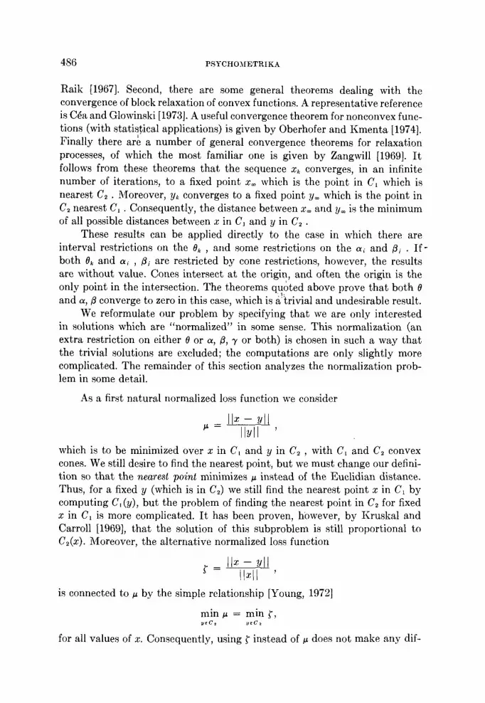
We reformulate our problem by specifying that we are only interestedin solutions which are "normalized" in some sense. This normalization (anextra restriction on either 0 or a, ~, ~ or both) is chosen in such a way thatthe trivial solutions are excluded; the computations are only slightly morecomplicated. The remainder of this section analyzes the normalization prob-lem in some detail.

As a first natural normalized loss function we consider

which is to be minimized over x in C~ and y in C= , with C~ and C~ convexcones. We still desire to find the nearest point, but we must change our defini-tion so that the nearest point minimizes u instead of the Euclidian distance.Thus, for a fixed y (which is in C~) we still find the nearest point x in C, computing C, (y), but the problem of finding the nearest point in C~ for fixedx in C, is more complicated. It has been proven, however, by Kruskal andCarroll [1969], that the solution of this subproblem is still proportional toC=(x). Moreover, the alternative normalized loss function

= -

is connected to ~ by the simple relationship [Young, 1972]

min~ = min~,

for all values of x. Consequently, using ~ instead of ~ does not make any dif-

JAN DE LEEUW, FORREST W. YOUNG AND YOSI-IIO TAKANE 487

ference. If we combine the results of Kruskal and Carroll with the fact thatfor any convex cone C it is true that C(o~x) = aC(x) for all a _> 0, we findthe important result that our previous alternating projection proceduresalso minimize the same subproblems for properly normalized loss functions.Moreover, the normalizing can be done whenever we want to; it is not neces-sary to normalize after each iteration, although we do. Finally, it does notmatter which of the two natural normalizations of k we use, as the resultsin each iteration will differ only by a proportionality factor, and the ultimatesolutions will always be identical. Observe that an equivalent formulationof the normalized problem is the maximization of the product of x and yunder the condition x ~ Cl , y ~ C2 , and under the normalization conditionsIlxll = 1 and IlYll = 1. This shows that we minimize the angle between thevectors x and y in their cones, without paying attention to their length.An alternative elementary proof of the Kruskal and Carroll results, withapplications to ALS, is given by de Leeuw [Note 4]. Convergence for nor-malized iterations follows in the same way as before from the general con-vergence theorems for relaxation processes.

It should be noted that we have not proven that our algorithm con-verges to the globally optimal point, only that it converges to a (perhapslocally) optimal point. It appears to the authors, however, that the algorithmnearly always obtains the global optimum, an assertion supported by someevidence presented in the results section. As will be discussed in the nextsection, ADDALS necessarily obtains the global optimum in certain specialcases.

Relation to Earlier Worl¢

When the data are discrete-nominal and when there are no restrictionson a~ and ~ , then the projections C~ and C2 are independent of x and y.Thus, there are orthogonal projection matrices A and B such that

y~÷~ = Bx, = BAy~ ,

and

x,+~ = Ay~+~ = ABx,.

It follows that in this case our ALS method is equivalent to the power methodfor computing the dominant eigenvalue and corresponding eigenvector ofBA and AB. Since the method proposed by Fisher [1938], and rediscoveredby Hayashi [1952], Carroll [Note 2], and Nishisato [Note 7] finds the eigen-value/eigenvector pair of the same matrices, it is clear that ALS is equivalentto these methods in this special case. Although the previously proposedmethods are more efficient, ADDALS is assured of obtaining the globaloptimum (the dominate eigenvalue/vector) in this case. It should be notedthat some of the previous work involves proposals for obtaining additional

488 PSYCHOMETRIKA

subdominant eigenvalues and eigenvectors to yield a multidimensionalquantification. Our developments do not cover this possibility nor that ofinteraction terms in the ANOVA model, a development which has beentreated by Nishisato ]Note 7, Note 8] in the case of discrete-nominal data andunrestricted model parameters. A companion paper to our present work[Young, de Leeuw, & Takane, 1976] does treat this topic, however.

Our missing data technique has been proposed by Yates ]1933] in thecase in which there are no constraints on the model parameters and thenon-missing observations are known real numbers [see also Wilkinson, 1958].The iterative te6hnique has also been used by some authors as a compu-rationally convenient way to estimate parameters in unbalanced designs.It has been shown that the technique solves the least squares problem by aniterative method based on a regular splitting of the design matrix. The theoryof such methods has been studied by Berman and Plemmons [1974].

It is also interesting to study the relationship of ALS and gradientmethods, since Kruskal ]1965] has proposed a gradient method for continuousor discrete ordinal data, with no constraints on the model parameters. Wefirst consider the general unnormalized problem of minimizing I Ix - Yll overx ~ C~ and y e C~. It is well known that the function

v(x) = min [Ix - y]~ = ~x - C~(x)[[,

is continuously differentiable, with gradient vector x - C~(x). The gradientprojection method [Levitin & Polyak, 1966] sets

x+ = C,[x - K(x - C~(x))],

with the step size K chosen in such a way that sufficient decrease of v(x) isguaranteed. Levitin and Polyak show that K = 1 is an admissible step size,and by setting K = 1 in the update equation we find the ALS method x+ =C~(C~(x)). Thus, our ALS algorithm is a convergent gradient projectionalgorithm ~vith constant step size. In the normalized case we find v(x), suchthat

v(x) = min ~x -- y~ ~[x -- C~(x)[[

which is continuously differentiable if ]]x[] ~ 0, with gradient

~(~) = llxlV’(x C~(x)) - ~(x) x.

Again, we can choose the stepsize in ~ gradient projection algorithm in sucha w~y that it becomes equivalent to ALS, except possibly for a differentnormalization of intermediate solutions. If one of the cones in the normalizedproblem is a linear subspace, we can collect a basis for the subspace in T,


and minimize

v(x) = min ~_Tx_-

unconditionally over x. Kruskal’s MONANOVA [1965] is the special case inwhich C~ is the polyhedral convex cone of monotone transformations. In thesame way as before, we show that the iterations of ALS can be intepreted(up to proportionality factors) as gradient iterations, with a particularchoice of the step size. In MONANOVA the step size is determined by acompletely different procedure, which may or may not be more efficient.

In a paper dealing with another special case of our situation, Bradley,Katti and Coons [1962] define

u(y) = rain ~- ~

and minimize u(y) over C~ by a coordinate descent method. The relationshipof this method and ALS is complicated, although the basic idea of decompos-ing the optimization problem in a cyclic sequence of simpler problems isthe same for both methods. If follows from the convergence theory of themethods we have shown to be equivalent to our method that convergenceof ALS in these cases is at most linear (and can degenerate to convergence oforder zero in some cases). In the computational literature a large number ofmethods are available that can be used to speed up convergence. In particular,our analysis shows that choosing a different step size in gradient projectionmethods corresponds to over or underrelaxing the ALS iterations. Our ex-amples show that in some instances convergence of ALS is quite slow, andthat experimenting with a relaxation parameter may be quite useful.

~. Results and Discussion

In this section we present the results of applying ADDALS to severalsets of data whose structures have been investigated by methods whichare special cases of ADDALS. For these data we expect our results to bevery much like the previous results. We also present the results of ADDALSanalysis of artificial data to evaluate other special ADDALS cases. We willfirst discuss nominal data, then ordinal, then numerical.

Nominal Data

Due to the equivalence of the iterative ADDALS method and the ana-lytic eigenvector method when the data are discrete-nominal, it is unneces-sary to determine whether ADDALS will behave robustly with artificialerror-free data, as it will. However, we should point out certain types ofdiscrete-nominal data (with or without error) which do not yield resultswhich are unique up to a linear transformation. An obvious example is data

490 PSYCHOMETRIKA

which consist of unique categories, i.e., for which there is only one observationin each category. For such data, any parameterization of ai and ~ yields aperfect, but meaningless, solution. A necessary condition for a unique solution,then, is that one category contains at least two observations. This condition isby no means sufficient, however. Consider, for example, the 3 X 3 tablewith 3 observations in each of 3 categories:

A A A

B B B-

C C C

In this case the row effects are completely indeterminate and the columneffects are only determined to be equal at all levels. As another, more subtleexample, consider the 3 X 4 table with eight observations categories:

A D B E

B E C F.

C F G H

If these categories are assumed to be discrete (not continuous), then the rowsare connected (since each shares categories with another row), but the columnsare only partially connected (since Column 1 shares categories only withColumn 3, and Column 2 only with Column 4). Thus, the rows are deter-mined up to a linear transformation, but the columns are determined upto two separable transformations, one for Columns 1 and 3, and anotherfor Columns 2 and 4, due to the fact that Columns 2 and 4 share no categorieswith Columns 1 and 3. Thus, an important condition to obtain results definedat the interval level from discrete-nominal data is that all rows (columns)be connected by common categories. It does not seem to be necessary that arow (column) share at least one category with all other rows (columns),but rather that a row (column) share at least one category with a secondrow which shares a category with a third, etc. Of course, these are but ex-amples, and we do not mean to imply that they represent a complete argu-ment for a necessary, let alone a sufficient condition which must be met toobtain a quantitative analysis. In the case of replicated data, for example,the condition given above can undoubtedly be weakened.

We have found that ADDALS yields results which are within a lineartransformation of those obtained by the analytic eigenvector procedurefor discrete-nominal data which meet the necessary condition given above.Fisher [1938, pps. 285-298] demonstrated his eigenvector method by analyz-ing data concerning twelve samples of human blood tested with twelve sera,where the observations were one of five chemical reactions (this is a balanced,unreplicated 12 X 12 factorial design with 5-category data assumed by


Fisher and ourselves to be discrete). ADDALS obtained a solution withk -- .5397 in 8 iterations with a random start. (The criterion to terminatethe iterative process in this and all other analyses, unless otherwise stated,is that the improvement in ks must be less than .0005.) The ADDALS param-eter estimates are related to Fisher’s estimates by a perfectly linear transfor-mation. Carroll [Note 2] demonstrated his CCM method (which is identicalto Fisher’s proposal) with data obtained in an experimental situationdescribed by three variables: the wave form, modulation percentage andmodulation frequency of a tone. The experimental design was a factorial2 X 3 × 4, balanced and unreplicated. The data analyzed by Carroll werethe five clusters into which each of the 24 tones were placed by a clu~teringprogram. Our analysis (assuming discrete process) yielded results indis-tinguishable from Carroll’s analysis, except for a linear transformation(~, = .4477, 34 iterations, random start).

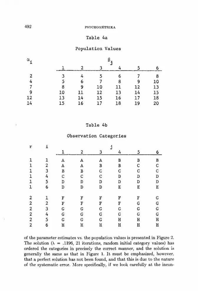
We now investigate the behavior of ADDALS using an artificial examplein which the true population values underlying the discrete-nominal obser-vations are known. In Table 4a we present the population values for theexample, and in Table 4b we present the observation categories (this is 6 X 6 balanced design with 2 replications, having 5 observation categoriesin the first replication and 3 different observation categories in the second).The population values are completely connected. In Table 4b we have in-troduced two types of systematic observation error. First, the true valueshave been collapsed into a smaller number of observation categories; second,there are inconsistencies (between replications) in the observation categories.However, there is no random error (the true values can be ordered properlyby the observation categories in each replication). These types of systematicerrors are common types of observational error in practice.

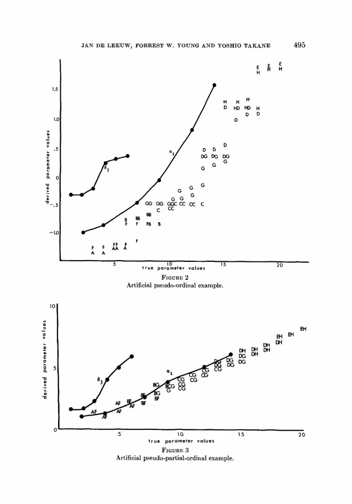
In Figure 1 we plot the parameter estimates obtained by ADDALS(~ = .3366 in 12 iterations, random initial category values) against the truevalues (the letters indicate category membership). It is clear that the deriveda~ are linearly related to their true values, though the ~ are not. In particular,the derived values of ~ and 2~ are equal even though the true values are not.This anomaly is due to the fact that the corresponding columns of the obser-vation matrix are identical. We note now that this effect carries through allthe analyses of these data which are to be presented, and that a linear relationcould be obtained ~vith differing observation columns. Identical columns(or rows) of observations is of some concern, however, and should be treatedwith caution.

In the remainder of this section we investigate the behavior of ADDALSunder the continuous-nominal assumptions. Actually, as noted above, thetotally unrestricted form of the continuous-nominal assumptions are meaning-less, so we impose the additional pseudo-ordinal restrictions discussed above,and then reanalyze the data in Table 4 under these restrictions. The plot

0 o

o C o


1.5

|.C

-a 0

-1.0

~DDOE E

H ~fH HH HH HDD D

/

C CCCCC CC C

J B BE, BBB B

F F FF FF FF ~ F

AA A10 . r 155 true parome~e values

Fmua~, 1Artificial d~scret, e-nominM example.

20

sistencies between the five observation categories for the first replication andthe three observation categories for the second replication, we note thatthere is no order of all eight observation categories which will permit a perfectsolution. Observation category G corresponds with the true values rangingfrom 8 through 15, whereas category B has observations which correspondto true values as large as 9, and category D has corresponding true valuesas small as 13. Thus, we see that we must define a partial order of thecategories in order to obtain a perfect fit (~ = 0), the partial order being

A <_B<_C<_ D<_E,

F<_G<_H,I,’ <_C,

G<E.

Since the pseudo-ordinal and ordinal assumptions do not permit partialorders (as stated above), we cannot perfectly fit these data. Thus, if we wereto now use the ordinal information developed by the pseudo-ordinal analysis

494 PSYCHOMETRIKA

to order all eight categories, and then use this information as the basis of acontinuous-ordinal analysis, we should still arrive at precisely the sameimperfectly fitting solution. Of course it would be relatively trivial to extendthe notions of the pseudo-ordinal and ordinal types of measurement to include(pseudo) partial orders, and in fact we have done so in some other closelyrelated work [Young, Note 9; Young, de Leeuw & Takane, 1976]. If we thenreanalyze these data under the assumption that they represent a pseudo-partial order, with the prior knowledge that the pseudopartial order consistsof two partial orders (one for the first replication, and one for the second),then we should certainly obtain a perfect fitting solution, questioning onlythe nature of the relationship of the solution to the true values. We haveperformed such as analysis using the multiple optimal regression by alter-nating least squares (MORALS) technique reported by Young, de Leeuw,and Takane [1976], which is precisely equivalent to ADDALS for orthogonalANOVA designs, except for the ability of MORALS to handle partial orders.The procedure obtained a perfect fit (2 iterations, random start). The derivedparameter values are plotted versus the true values in Figure 3. The figureindicates that the dependent variable and the values of ai are essentiallylinear in their relationship to the true values, and that ~i still displays thesame nonlinearities as before, but more mildly. The usefulness of such aprocedure might be questioned since it assumes that we have prior knowledgeabout the nature of the partial order (that we know it consists of two sub-orders). However, it is often the case that the observation categories in onereplication of the experiment bear no simple relationship to the observationcategories in another replication. In such a situation the (pseudo) orderreally consists of several sub-orders, one for each replication.

We conclude, then, that under the appropriate conditions ADDALScan yield quantitative analyses of nominal data. It seems clear that onenecessary condition is that all rows (columns) be connected by commoncategories, and it is probably the case that the number of observation shouldbe large relative to the number of categories. For the latter reason it is desir-able to have as many replications as possible. Finally, some care should beexercised when a) two or more (columns) are identical, since this necessarilymeans the parameter estimates will be equal; and b) the data are pseudo-ordinal, since the parameter restrictions are so ~veak.

Ordinal Data

Our first ordinal example utilizes an artifical example discussed byKruskal [1965] in his paper concerning MONANOVA. His 3 X 3 data arethe squares of the "true" values obtained by the simple addition of the popula-tion row and column values. Thus, his data contain only systematic error.Furthermore, his population values have completely connected rows andcolumns. The ADDALS analysis of these data obtained a solution with

1.5

1.C

JAN DE LEEUW~ FORREST ~V. YOUNG AND YOSHIO TAK~kNE

HD

D

CC CC C

5 10 15true parameter values

F~GURE 2

Artificial pseudo-ordinal example.

HHHD HD H

D DD

495

2O

10

EH EHEH

true parameter values

FIGURE 3

Artificial pseudo-partial-ordinal example.

~5 2O

496 PSYCHO.~IETRIKA

h = .0000 in 5 iterations (the discrete-ordinal assumption was used). Sincethis result might have been an artifact of the "rational start" (i.e., the obser-vations were used to initialize the algorithm), we repeated it with a randomstart, obtaining ~ = .0000 in 8 iterations. Both solutions are indistinguishableand are perfectly related to the underlying structure.

We felt that the results reported in the previous paragraph might bedue to the strong connectedness of the data (and the assumption of discreteobservations), so we analyzed a second set of 3 X 3 artificial discrete-ordinaldata which have one unconnected column. The results of this analysis wereessentially identical to those of the first analysis (~ = .0000, in 5 iterationsfrom a rational strat and 12 iterations from a random start, estimates per-fectly related to true values). We pushed this notion even further by analyzinga third set of identical 3 X 3 discrete-ordinal data for which one row and onecolumn are unconnected. In this case the analysis suffered, with the under-lying structure not perfectly recovered (although ~ = .0000 in 4 iterationsfor rational start). So, again, it is important to have connected rows andcolumns, especially for unreplicated matrices as small as the one analyzedhere. Of course, if we had assumed the data were continuous-ordinal ourresults would have been less encouraging for these 3 X 3 matrices, since thiseffectively disconnects any connections which may be present in the data.(We also performed all the previous analyses with Kruskal’s MONANOVAand obtained indistinguishable results.)

Kruskal [1965] used several sets of real data to evaluate his procedure.We reanalyzed two of these sets to further evaluate ADDALS (both of thesesets have also been analyzed by Box & Cox, 1964). The first of these twosets of data concern the strength of yarns (in terms of the number of cyclesbefore failure) when the amount of load placed on the yarn, the amplitudeof the load cycle, and the length of the piece of yarn are varied. Each ofthe three variables had three levels, and one observation was obtained ineach cell. Thus, this is a balanced, unreplicated 3 X 3 X 3 design. In keepingwith Kruskal’s analysis, we assume that the observations are continuous-ordinal and the experimental conditions are nominal. These data were sub-mitted to ADDALS and to Kruskal’s MONANOVA procedure. After 7iterations, ADDALS had converged to a value of ~, = .071, and after 8 itera-tions MONANOVA had converged to the same value. Both proceduresobtained solutions identical up to a linear transformation.

The second set of Box and Cox data analyzed by Kruskal concern thesurvival time of animals subjected to one of three poisons and one of fourtreatments. These data were obtained from four animals in each condition;thus the experiment is a balanced, 3 X 4 design with four replications. Theresults of our analysis, which assumed that the observations were continuousand that the experimental variables were nominal, were compared with theresults of Kruskal’s analysis (which made the same assumptions) Again,


the results are virtually identical: ADDALS ~ = .3064 on the sixth iteration,MONANOVA ~ = .3064 on the eighth.

By removing some of the observations from these data, we obtain anunbalanced design whose analysis can be compared with the analysis of thebalanced design. Thus, we removed four of the 48 observations, one from eachof the three cells involving the fourth level of the treatment variable, andone from cell 1, 1. This leaves us with an unbalanced 3 X 4 design with fourreplications in eight of the 21 cells and three replications in each of the re-maining four cells. When we compare the results of this analysis with thoseof the previous one, we see that the estimates have changed somewhat. Wealso note that the value of ~ (.2751 in 5 iterations) has decreased some fromthe balanced case, suggesting that its value is a function of the number ofobservations (as is the case in a closely related situation discussed by Young,1970). Finally, we note that the observations have been removed from thebalanced design in such a way that two columns have no observationsremoved, one column has one observation removed, and one column has threeobservations removed. The number of observations removed is related tothe degree of change in the corresponding parameter’s estimate. Specifically,the column parameter estimate which changed the most is the one with thelargest number of observations removed.

We now turn to two examples involving ordinal constraints on theexperimental variables. Roskam [1968], in demonstrating his ADDIT proce-dure (which is nearly identical to Kruskal’s MONANOVA), used a set data gathered by Ekman [Note 5] concerning the average ratings of un-pleasantness of an electrical shock whose intensity and duration was varied,involving 5 and 6 levels of each variable. We analyzed these data assumingthat the experimental variables were ordinal and the measurement processwas continuous-ordinal. When we compared our results (~ = .0100 in iterations) with Roskam’s (who was unable to assume ordinal effects, andso treated them as nominal), we concluded that the two analyses were highlysimilar (all a~ and ~i were identical for both analyses except two values whoseorder was "incorrect" for the unrestricted analyses). This implies that theassumption of ordinal effects was appropriate, though unnecessary, and thatit had no deleterious effects on the analysis.

As a second example of imposing ordinal constraints on experimentalvariables, we analyzed data gathered by Kempler [1971] concerning thenumber of times each of 100 rectangles was judged to be either large or smallby several subjects. The variables are the height and width of the rectangles;each variable has 10 levels. We analyzed these data both with and withoutthe ordinal constraints on the two experimental variables. Without ordinalconstraints we (and Kempler) discovered a few inversions from the expectedorder. We note that the value of h increased from. 1558 for the unconstrainedanalysis (5 iterations) to. 1565 for the constrained analysis (also 5 iterations),

498 PSYCHO.~[ETRIKA

a very slight increase due to the restraints. Thus, this aspect of ADDALSallows us to observe that the best fitting constrained estimates (and theiroverall descriptive adequacy) are nearly as adequate as the free estimates.

Finally, we reanalyzed the artificial data in Table 4 under the assumptionthat the categories were continuous-ordinal, with the ordinal informationbeing derived from the pseudo-ordinal analysis. The results were identicalto those of the pseudo-ordinal analysis (), = .1196, all parameters the sameto four decimal places). The only difference was that less iterations ~vererequired; this was due, apparently, to the non-random initial category values.This lends some credence to the pseudo-ordinal procedure. We also analyzedthese data under the partial order assumptions discussed above, and obtainedprecisely the same solution as obtained with the pseudopartial order assump-tions.

Numerical Data

It is unnecessary, of course, to give an example of ADDALS applied todiscrete-numerical data, since ADDALS reduces to computing row andcolumn means of the data matrix i,n this case. Furthermore, with discretenumerical data which have missing observations ADDALS is equivalentto the iterative missing data technique proposed by Yates [1933], and thereare many examples analyzed by this technique in the analysis of varianceliterature. Thus we will not discuss the discrete-numerical case, but turninstead to the continuous-numerical case.

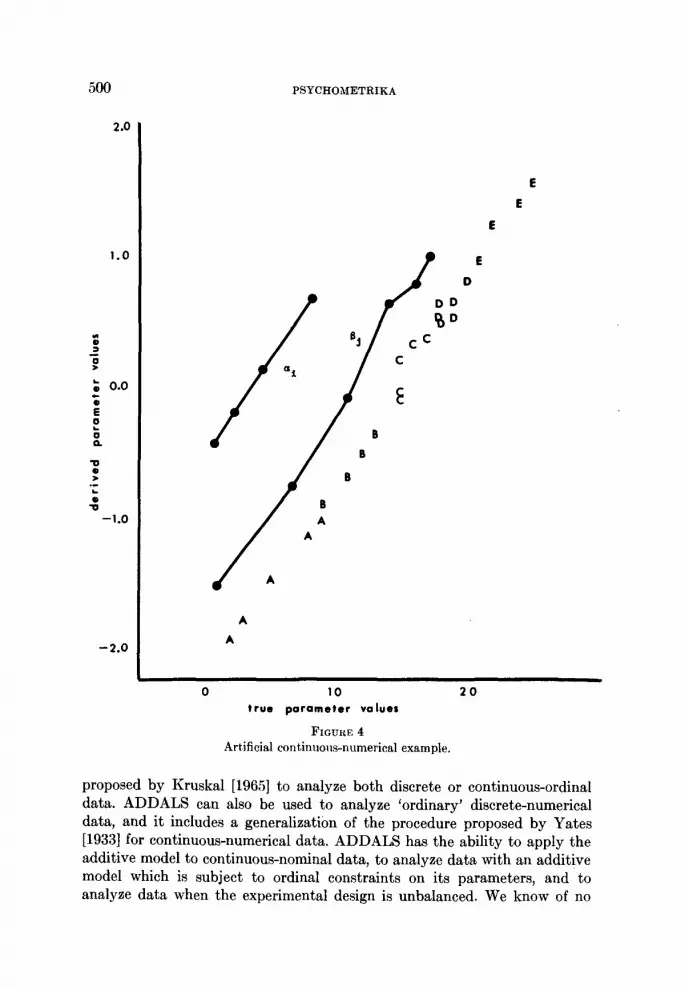
We cannot compare our method with previous ones in the continuous-numerical case since we know of none, so we evaluate this case by analyzinga set of artificial data. In Table 5a we present the population values; inTable 5b the observation categories and the category constraints are dis-played. This example contains errors of observation similar to those in Table 4(there are fewer observation categories than population values), but therange constraints are such that the population values constitute a perfectsolution. Note that this example is quite strong in that all rows and columnsof the population matrix are connected.

The parameter estimates obtained by the ADDALS analysis of thesedata are plotted against the population values in Figure 4. We observe thatthe estimates of the four row parameters a~ are, essentially, a perfect lineartransformation of their population values. We also observe that the estimatesof the six column parameters Bi are related by the same linear transformationto their population values, but that this latter relationship is not perfect.(Of course, when we plot the dependent variable we see the same linear,imperfect relationship.) In particular, we note that the fourth largest columnestimate is relatively imprecise. We are unsure why this is the case, but wedo note that convergence is very slow for this example (38 iterations beforethe convergence criterion of .00005 was met), and that the solution, at this

JAN DE LEEUW, FORREST W. YOUNG AND YOSHIO TAKANE

Table 5a

Population Values

i 7 ii 14 16 17

1 2 8 12 15 17 182 3 9 13 16 18 194 5 ii 15 18 20 218 9 15 19 22 24 25

499

Table 5b

Observations

ii 2 3 4 5 6

i A A B C C D2 A A B C D D3 A B C D D E4 B C D E E E

Constraints

2 < A < 9 < B < 13 < C < 17 < D < 20 < E < 25

point, does not yet fit perfectly (~ = .0050). Perhaps if we had let ADDALSrun for more iterations an improved solution would be obtained. We do feel,however, that this example indicates that with continuous numerical dataADDALS can behave in a relatively efficacious manner.

5. Conclusions

We conclude that the ADDALS approach enables one to quantifyqualitative data via the application of the additive model (subject to condi-tions discussed in the previous section). Furthermore, we conclude that theassociated algorithm is simple and efficient, in terms of both speed and size.We note that ADDALS includes, as special cases, the procedure first proposedby Fisher [1938] to analyze discrete-nominal data and the procedure first

5OO

2,0

1.0

--2.0

PSYCHO~ETRIKA

BA

A

B

C

A

A

CC

DD

0 10 20true parameter values

F~GUR~ 4Artificial continuous-numerical example.

proposed by Kruskal [1965] to analyze both discrete or continuous-ordinaldata. ADDALS can also be used to analyze ’ordinary’ discrete-numericaldata, and it includes a generalization of the procedure proposed by Yates[1933] for continuous-numerical data. ADDALS has the ability to apply theadditive model to continuous-nominal data, to analyze data with an additivemodel which is subject to ordinal constraints on its parameters, and toanalyze data when the experimental design is unbalanced. We know of no


previous proposals which cover any of these last developments. Thus, weconclude that ADDALS is a procedure which is much more general andflexible than previous proposals.

Finally, it is fairly simple to generalize the approach to models otherthan the simple additive model. Research recently completed suggests thatthe alternating least squares approach can be generalized in a. straight-forward manner to other linear models. We have already developed robust(and rapid) ALS procedures to apply the multiple and canonical correlationmodels to nominal and ordinal variables [Young, de Leeuw & Takane, 1976].Special cases of this procedure include Procrustean rotation, external un-folding, vector projection, additive models with interaction terms, non-orthogonal models, ADDALS, etc. An ALS procedure has also been developedand evaluated for the bilinear model which includes nonmetric (and, of course,nominal) factor analysis, components analysis, etc., as special cases. Atthe time of this writing, this development appears to yield a robust andrapid method. Finally, we have extended the ALS methodology to the bi-quadratic models (the Euclidian and weighted Euclidian models) commonlyused in multidimensional scaling [Takane, Young, and de Leeuw, in press].Although this is considerably more complex than those just mentioned, itdoes appear to provide a promising alternative to the commonly used proce-dures. Thus, we find ALS methodology encouraging not only because of itsability to quantify qualitative data via application of the additive model,but also because of its promise to quantify qualitative data via applicationof a variety of other models.

REFERENCE NOTES

1. Bock, R. D. Methods and applications of optimal scaling (L. L. Thurstone PsychometricLaboratory Report No. 25). Chapel Hill, North Carolina: The L. L. Thurstone Psycho-metric Laboratory, University of North Carolina, 1960.

2. Carroll, J. D. Categorical conjoint measurement. Unpublished paper, Bell TelephoneLaboratories, Murray Hill, New Jersey, 1969.

3. de Leeuw, J. The linear nonmetric model (Report RN003-69). Leiden, the Netherlands:University of Leiden, 1969.

4. de Leeuw, J. Normalized cone regression. Unpublished paper, Department of DataTheory, University of Leiden, 1975.

5. Ekman, G. The influence of intensity and duration of electrical stimulation on subjectivevariables (Report 17A). Stockholm:Psychological Laboratory, University of Stockholm,1965.

6. Kruskal, J. B. and Carmone, F. Use and theory of MONANOVA, a progra~n to analyze.factorial experiments by estimating monotone transformation of the data. Unpublishedpaper, Bell Telephone Laboratories, Murray Hill, New Jersey, 1968.

7. Nishisato, S. Optimal scaling and its generalizations, I: Methods (Report 1). Toronto:Ontario Institute for Studies in Education, Department of Measurement and Evalua-tion, 1972.

8. Nishisato, S. Optimal scaling and its generalizations, II: Applications. Toronto: OntarioInstitute for Studies in Education, Department of Measurement and Evaluation, 1973.

502 PSYCHOMETRIKA

9. Young, F. W. Conjoint scaling (L. L. Thurstone Psychometric Laboratory ReportNo. 118). Chapel Hill, North Carolina: The L. L. Thurstone Psychometric Laboratory,University of North Carolina, 1973.

REFERENCES

Barlow, R. E., Bartholomew, D. J., Bremner, J. M., and Brunk, H. D. Statistical inferenceunder order restrictions. London: Wiley, 1972.

Barlow, R. E. and Brunk, H. D. The isotonic regression problem and its dual. Journal ofthe American Statistical Association, 1972, 67, 140-147.

Berman, A. and Plemmons, R. J. Cones and iterative methods for best least squaressolutions of linear systems. SIAM Journal of Numerical Analysis, 1974, I1, 145-154.

Box, G. E. P. and Cox, D. R. An analysis of transformations. Journal of the Royal StatisticalSociety, Series B, 1964, 26, 211-252.

Bradley, R. A., Katti, S. K., and Coons, I. J. Optimal scaling for ordered categories.Psychometrika, 1962, 27, 355-374.

Butt, C. The factorial analysis of qualitative data. British Journal of Statistical Psychology,1950, 3, 166-185.

Cea,J. and Glowinski, R. Sur des methodes d’optimisation par relaxation. Revue Francaised’Automatique, Informatiquc, et Recherche Op~rationelle, section R3, 1973, 7, 5-32.

Corsten, L. C. A. and van Eynsbergen, A. C. Multiplicative effects in two-way analysisof variance. Statistica Neerlandia, 1972, 26, 61-68.

de Leeuw, J. Canonical analysis of categorical data. Leiden, The Netherlands: Universityof Leiden, 1973.

Fisher, R. A. Statistical methods for research workers. Edinburgh: Oliver and Boyd, 1938(7th printing), 1946 (10th printing).

Gubin, L. G., Polyak, B. T., and Raik, E. V. The method of projections for finding thecommon point of convex sets. U.S.S.R. Computational and Mathematical Physics,1967, 7, 1-24.

Guttman, L. The quantification of a class of attributes: A theory and method of scaleconstruction. In P. Horst (Ed.), The prediction of personal adjustment. New York:Social Science Research Council, 1941.

Hayashi, C. On the predictions of phenomena from qualitative data and quantificationsof qualitative data from the mathematico-statistical point of view. Annals of theInstilule of Statistical Mathematics, 1952~ 3, 69-92.

JSreskog, K. G. Some contributions to maximum likelihood factor analysis. Psychometrika,1967, 32, 443-482.

Kempler, B. Stimulus correlates of area judgments: A psychological developmental study.Developmental Psychology, 1971, 4i, 158-163.

Kruskal, J. B. Analysis of factorial experiments by estimating monotone transformationsof the data. Journal of the Royal Statistical Society, Series B, 1965, 27, 251-263.

Kruskal, J. B. Nonmetric multidimensional scaling: A numerical method. Psychometrika,1964, 29, 28-42.

Kruskal, J. B. and Carroll, J. D. Geometric models and badness-of-fit functions. In P. R.Krishnaiah (Ed.), Multivdriate Analysis II. New York: Academic Press, 1969.

Levitin, E. S. and Polyak, B. T. Methods of minimization under restrictions. U.S.S.R.Computational and Mathematical Physics, 1966, 6, 1-50.

Lingoes, J. C. The Guttman-Lingoes nonmetric program series. Ann Arbor, Michigan:Mathesis Press, 1973.

Oberhofer, W. and Kmenta, J. A general procedure for obtaining maximnm likelihoodestimates in generalized regression models. Econometrica, 1974, $2, 579-590.

JAN DE LEEUW~ FORREST W. YOUNG AND YOSHIO TAKANE 503

Purl, M. L. & Sen, P. K. Nonparametric methods in muttivariate analysis. New York:Wiley, 1971.

Roskam, E. E. Ch. [. Metric analysis of ordinal data in psychology. Voorschoten, Holland:VAM, 1968.

Takane, Y., Young, F. W., and deLeeuw, J. Nonmetric individual differences multidimen-sional scaling: An alternating least squares method with optimal scaling features.Psychometrika, in press.

Wilkinson, G. N. Estimation of missing values for the analysis of incomplete data. Bio-metrics, 1958, 14, 257-286.

Wold, H. & Lyttkens, E. (Eds.). Nonlinear iterative partial least squares (NIPALS)estimation procedures (group report). Bulletin of the International Statistical Institutc,1969, 43, 29-51.

Yates, F. The analysis of replicated experiments when the field results are incomplete.The Empire Journat of Experimental Agriculture, 1933, I, 129-142,

Young, F. W. A model for polynomial conjoint analysis algorithms. In R. N. Shepard,A. K. Romney, and S. Nerlove (Eds.), Multidimensional scaling: Theory and applica-tions in the behavior-sciences. New York: Academic Press, 1972.

Young, F. W. Nonmetric multidimensional scaling: Recovery of metric information.Psychometrika, 1970, 35, 455-473.

Young, F. W., de Leeuw, J. & Takane, Y. Regression with qualitative and quantitativevariables: An alternating least squares method with optimal scaling features. Psycho-metrika, 1976, 41,000-000.

Zangwill, W. I. Convergence conditions for nonlinear programming algorithms. Manage-ment Science, 1969, 16, 1-13.

Manuscript received 6/16/75Final version received 11/25/75

Documents

Additive structure in qualitative data: An alternating least squares method with optimal scaling features