Adaptive extended Kalman filter for geo-referencing of a TLS-based multi-sensor-system

TS number – Session title (e.g. TS 1A – Standards ) Comm. 5

Jens-André Paffenholz, Hamza Alkhatib and Hansjörg Kutterer

Adaptive Extended Kalman Filter for Geo-Referencing of a TLS-based Multi-Sensor-System

FIG Congress 2010

Facing the Challenges – Building the Capacity

Sydney, Australia, 11-16 April 2010

1/15

Adaptive Extended Kalman Filter for Geo-Referencing of a TLS-Based

Multi-Sensor-System

Jens-André PAFFENHOLZ, Hamza ALKHATIB and Hansjörg KUTTERER, Germany

Key words: terrestrial laser scanning, geo-referencing, extended Kalman filter

SUMMARY

This paper works on an adaptive extended Kalman filter (AEKF) approach for geo-

referencing tasks for a multi-sensor system (MSS). The MSS is built up by a sensor fusion of

a phase-based terrestrial laser scanner (TLS) with navigation sensors such as, e.g., Global

Navigation Satellite System (GNSS) equipment and inclinometers. The position and

orientation of the MSS are the main parameters which are constant per station and will be

derived by a Kalman filtering process. However, by inclinometer measurements the spatial

rotation angles about the X- and Y-axis of the fixed MSS station can be respected in the

AEKF. This makes it possible to respect all 6 degrees of freedom of the transformation from a

sensor-defined to a global coordinate system. The paper gives a detailed discussion of the

strategy for the direct geo-referencing. The AEKF for the transformation parameters

estimation is presented with the focus on the modeling of the MSS motion. The potential of

the strategy will be shown by practical investigations as well as an overview about the

observation and GNSS analysis strategy will be given.




FIG Congress 2010



2/15

Adaptive Extended Kalman Filter for Geo-Referencing of a TLS-Based

Multi-Sensor-System

Jens-André PAFFENHOLZ, Hamza ALKHATIB and Hansjörg KUTTERER, Germany

1. INTRODUCTION

The characteristic of the terrestrial laser scanning technique established nowadays in the

engineering geodesy is the immediate data acquisition in 3D space. This is realized with a

high spatial resolution as well as with a very high frequency in a relative or local sensor-

defined coordinate system, respectively. The terrestrial laser scanning technique can be

divided into static and kinematic scanning. The static scanning is characterized by one single

fixed translation and orientation of the terrestrial laser scanner (TLS) in relation to an absolute

or global coordinate system. For the kinematic scanning, where the data acquisition is

commonly reduced to 2D profiles, the translation and orientation is time-dependent. Hence

the transformation parameters for each profile are different in relation to each other as well as

to an absolute or global coordinate system. Typically the transformation parameters are

observed by navigation sensors and are estimated in a Kalman filtering process [Vennegeerts

et al., 2008].

These properties –the observation of transformation parameters and the Kalman filtering

process– will be transferred to the static scanning domain for registration and geo-referencing

tasks of 3D laser scans. Whenever a combination of several scans from different stations into

one coordinate system (registration) is required, the transformation parameters for each scan

have to be estimated. These parameters can be estimated by iterative algorithms, e.g., the

Iterative Closest Point (ICP) algorithm [Besl & McKay, 1992], or by identifying several

artificial control points in each scan. For an additional link to an absolute or global coordinate

system (geo-referencing), control points with a known geodetic datum are indispensible. In

case of the geodetic datum of the control points has also to be determined, the procedure

would be complex and time-consuming due to an extra and independent surveying.

It is possible, however, to transfer the above mentioned properties from the kinematic

scanning domain to the static scanning. First there is the direct observation of the position and

orientation, which can be derived by the orbital motion of the fixed laser scanner station.

Therefore a multi-sensor system (MSS) is created by a laser scanner and navigation sensors,

which is comparable to the setup of a MSS for kinematic scanning applications, called mobile

mapping system [Vennegeerts et al., 2008]. Afterwards a Kalman filtering process is initiated

for the estimation of the transformation parameters, which are constant for the whole 3D laser

scan. These parameters may also be used as appropriate start values with variance information

for iterative algorithms for registration tasks without the need of any control points.

This short introduction shows already that the direct geo-referencing of static 3D laser scans

offers a number of great advantages over the traditional way by using control points.

https://www.researchgate.net/publication/220183320_A_Method_for_Registration_of_3-D_Shapes?el=1_x_8&enrichId=rgreq-80dd447d1e60550cc84b1a44a2fb7016-XXX&enrichSource=Y292ZXJQYWdlOzI2MjE0MzE2MztBUzo5NzI2NTczNzc5NzYzNUAxNDAwMjAxMzY3MzM1

https://www.researchgate.net/publication/240754400_Validation_of_a_kinematic_laserscanning_system?el=1_x_8&enrichId=rgreq-80dd447d1e60550cc84b1a44a2fb7016-XXX&enrichSource=Y292ZXJQYWdlOzI2MjE0MzE2MztBUzo5NzI2NTczNzc5NzYzNUAxNDAwMjAxMzY3MzM1






FIG Congress 2010



3/15

The paper is organized as follows. Section 2 describes the strategy for the direct geo-

referencing of a TLS-based MSS as well as the anew developed algorithm for estimation of

the transformation parameters. Section 3 briefly introduces the adaptive extended Kalman

filter (AEKF) for direct geo-referencing with its two main components: the kinematic

equation of the state and the measurements equation. Practical investigations of the anew

algorithm are presented in Section 4. Finally, Section 5 summarizes the results and gives an

outlook for future work.

2. STRATEGY FOR THE DIRECT GEO-REFERENCING OF A TLS-BASED MSS

In Section 1 the idea of a TLS-based MSS for direct geo-referencing purposes was briefly

outlined. The main aim of the direct geo-referencing strategy is the direct observation of the

required transformation parameters from the local sensor-defined coordinate system, given by

the MSS, to a global coordinate system. This 3D transformation is defined by a translation

vector, which is equal to the position of the MSS, and a rotation matrix, which contains the

orientation of the three axes of the MSS, comparable to roll, pitch and yaw angle known from

aeronautics. One can sum up that this transformation has at least 6 degrees of freedom (dof)

which have to be observed and estimated, respectively. However, 4 of the 6 dof, the position

vector as well as the azimuthal orientation (yaw), are essential. Because of the fixed terrestrial

MSS, which can be orientated to the center of gravity, the spatial rotations (roll and pitch)

about the X- and Y-axis of the MSS can be minimized.

In the following the strategy for the direct geo-referencing of a TLS-based MSS, which is

realized as an adapted sensor-driven method at the Geodetic Institute of the Leibniz

Universität Hannover (GIH), will be described. The strategy can be divided into a sensor

fusion part and a part which deals with the algorithm for the estimation of the transformation

parameters.

2.1 Senor fusion in the MSS

As already mentioned, the MSS is established by a sensor fusion of a phase-based TLS, which

is the main sensor, and other additional navigation sensors to observe the transformation

parameters. While creating the MSS, several terms have to be considered. So the operation of

the laser scanner should neither be restricted nor disturbed by any of the enlisted additional

sensors. Hence, one should take advantage of the individual characteristic of any sensor. Here

one can point out the usage of the constant rotation of the laser scanner about its vertical axis

as time and orientation reference. Due to the TLS characteristic of a high frequency data

acquisition rate with in general more than 10 Hz for the used phase-based TLS as well as to

get reliable transformation parameters, the availability of data rates of at least 10 Hz for the

additional sensors is required. Indispensable in the MSS is the synchronization of all different

sensors so that the individual measurements could be set in a temporal relationship to each

other. Therefore it is useful to introduce one unique time reference in the MSS. The most

suitable way in this MSS is to use the GPS time as reference because it is instantaneously

available due to the GNSS observations.




FIG Congress 2010



4/15

The minimum number for additional sensors is one GNSS equipment. The case of mounting

two GNSS antennas on top of the laser scanner leads to different approaches within the scope

of the GNSS analysis which will be discussed later on. Nevertheless, if one or two GNSS

antennas are used, the trajectory of an antenna reference point (ARP) is a space curve which is

described by the orbital motion of the laser scanner. For the first realization of a MSS for

direct geo-referencing at the GIH only GNSS equipment was used. This leads to the fact that

only 4 of the 6 dof are determinable. Additionally, a horizontally mounted MSS is assumed

and any residual divergence of the orientation to the center of gravity will be neglected. For

further details, especially about the time synchronization in the MSS, please refer to

[Paffenholz & Kutterer, 2008].

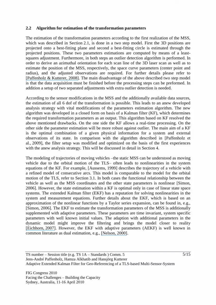
In order to optimize the direct geo-referencing strategy, some sensor modifications in the

MSS were carried out. In a first step the MSS is extended with additional navigation sensors –

inclinometers– to estimate the remaining 2 dof (the spatial rotations about the X- and Y-axis

of the MSS). Therefore two single axis inclinometers were mounted next to the GNSS

antenna on top of the laser scanner, each of them observing one spatial rotation about the X-

and Y- axis, respectively (see Figure 1). For synchronization purposes an external process

computer with integrated analogous-digital (A/D) converter is used. The topic of ongoing

investigations is to use the integrated inclinometer in the new laser scanner series. The

challenge of using the integrated inclinometers is the synchronization of the data because a

parallel way of synchronization to the external sensors is not possible at the moment.

Another modification of the MSS, unlike the strategy described in [Paffenholz et al., 2009],

was performed to the used data sources for the estimation of the transformation parameters.

As new input data the horizontal motor steps of the laser scanner were introduced to the

algorithm to get measured information about the orbital motion of the laser scanner. The

synchronization of this new data source is straightly available by the general synchronization

pulse of the laser scanner which corresponds to the progress in the horizontal rotation of the

laser scanner about its vertical axis.

The described sensor modification and additionally available data source lead to significant

modifications of the algorithm for the estimation of the transformation parameters. In

addition, and due to the consideration of all dof of the transformation from the local to the

global coordinate system, a more accurate estimation of the unknown parameters is expected.

Figure 1: Actual setup of the MSS equipped with one GNSS antenna and two external inclinometers

on top of a phase-based TLS

https://www.researchgate.net/publication/237453069_Direct_geo-referencing_of_a_static_terrestrial_laser_scanner?el=1_x_8&enrichId=rgreq-80dd447d1e60550cc84b1a44a2fb7016-XXX&enrichSource=Y292ZXJQYWdlOzI2MjE0MzE2MztBUzo5NzI2NTczNzc5NzYzNUAxNDAwMjAxMzY3MzM1




FIG Congress 2010



5/15

2.2 Algorithm for estimation of the transformation parameters

The estimation of the transformation parameters according to the first realization of the MSS,

which was described in Section 2.1, is done in a two step model. First the 3D positions are

projected onto a best-fitting plane and second a best-fitting circle is estimated through the

projected positions. These two parameters estimations are computed by means of a least-

squares adjustment. Furthermore, in both steps an outlier detection algorithm is performed. In

order to derive an azimuthal orientation for each scan line of the 3D laser scan as well as to

estimate the position of the MSS, respectively, the space curve parameters (center point and

radius), and the adjusted observations are required. For further details please refer to

[Paffenholz & Kutterer, 2008]. The main disadvantage of the above described two step model

is that the data acquisition must be finished before the processing steps can be preformed. In

addition a setup of two separated adjustments with extra outlier detection is needed.

According to the sensor modifications in the MSS and the additionally available data sources,

the estimation of all 6 dof of the transformation is possible. This leads to an anew developed

analysis strategy with vital modifications of the parameters estimation algorithm. The new

algorithm was developed in a closed form on basis of a Kalman filter (KF), which determines

the required transformation parameters as an output. This algorithm based on KF resolved the

above mentioned drawbacks. On the one side the KF allows a real-time processing. On the

other side the parameter estimation will be more robust against outlier. The main aim of a KF

is the optimal combination of a given physical information for a system and external

observations of its state. In comparison with the algorithm described in [Paffenholz et

al., 2009], the filter setup was modified and optimized on the basis of the first experiences

with the anew analysis strategy. This will be discussed in detail in Section 4.

The modeling of trajectories of moving vehicles –the static MSS can be understood as moving

vehicle due to the orbital motion of the TLS– often leads to nonlinearities in the system

equations of the KF. For example, [Aussems, 1999] describes the trajectory of a vehicle with

a refined model of consecutive arcs. This model is comparable to the model for the orbital

motion of the TLS, refer to Section 3.1. In both cases the functional relationship between the

vehicle as well as the MSS coordinates and the other state parameters is nonlinear [Simon,

2006]. However, the state estimation within a KF is optimal only in case of linear state space

systems. The extended Kalman filter (EKF) has a reputation for solving nonlinearities in the

system and measurement equations. Further details about the EKF, which is based on an

approximation of the nonlinear functions by a Taylor series expansion, can be found in, e.g.,

[Simon, 2006]. The EKF to estimate the transformation parameters of the MSS is additionally

supplemented with adaptive parameters. These parameters are time invariant, system specific

parameters with well known initial values. The adaption with additional parameters in the

dynamic model might improve the filtering and brings the model closer to reality

[Eichhorn, 2007]. However, the EKF with adaptive parameters (AEKF) is well known in

common literature as dual estimation, e.g., [Nelson, 2000].

https://www.researchgate.net/publication/229029295_Analysis_of_dynamic_deformation_processes_with_adaptive_KALMAN-filtering?el=1_x_8&enrichId=rgreq-80dd447d1e60550cc84b1a44a2fb7016-XXX&enrichSource=Y292ZXJQYWdlOzI2MjE0MzE2MztBUzo5NzI2NTczNzc5NzYzNUAxNDAwMjAxMzY3MzM1

https://www.researchgate.net/publication/36398455_Nonlinear_estimation_and_modeling_of_noisy_time-series_by_Dual_Kalman_filtering_methods?el=1_x_8&enrichId=rgreq-80dd447d1e60550cc84b1a44a2fb7016-XXX&enrichSource=Y292ZXJQYWdlOzI2MjE0MzE2MztBUzo5NzI2NTczNzc5NzYzNUAxNDAwMjAxMzY3MzM1





FIG Congress 2010



6/15

Figure 2: Schematic overview of the present strategy from the data acquisition to the estimation of the

transformation parameters




FIG Congress 2010



7/15

2.3 Schematic overview of the present strategy

In Figure 2 a schematic overview of the present strategy from the data acquisition to the

estimation of the transformation parameters is given. In order to simplify the complex strategy

the whole procedure is structured into five parts:

In part I the data acquisition of the MSS is summarized. The four sensor types are the GNSS

equipment in green, the terrestrial laser scanner with integrated inclinometer in blue, the

external inclinometer in red, and the real-time process computer with A/D converter also in

red. For each sensor type an individual pre-processing is performed. For the GNSS equipment

the analysis is performed by commercial software, e.g., Wa1 by Lambert Wanninger or

Geonap by Geo++®

. The line synchronization pulses of the laser scanner, registered with the

event marker input, are analyzed with respect to data gaps. The time stamp of the data is

already the MSS unique GPS time reference. For the TLS the raw values of the horizontal

motor steps are extracted from the stored 3D point cloud. They correspond to the number of

2D profiles within the 3D point cloud as well as to the number of line synchronization pulses.

It is also possible to get an on-the-fly access to the horizontal motor steps, which will be

realized in the ongoing work. The registered inclinations from the integrated sensor are not

processed because of the missing synchronization possibility as already described before. The

analogous data stream of the external inclinometers adapted on the laser scanner is processed

by the A/D converter of the real-time process computer. All incoming data streams to the real-

time process computer are marked with an internal time stamp of the process computer.

Besides the inclinations the pulse per second (PPS) signal and a National Marine Electronics

Association (NMEA) string, containing the UTC time information of the GNSS receiver, as

well as the line synchronization pulses are the input data of the real-time process computer.

The data delivered by the GNSS receiver is pre-processed in a way that for each PPS the

corresponding GPS time stamp is generated by the UTC information extracted from the

NMEA string. The line synchronization pulses are registered twice, once by the GNSS

receiver (event marker input) and once by the real-time process computer. The data stored by

the GNSS receiver is used for the further data processing and the other data source is used as

backup.

In part II the required data synchronization of the MSS is described. As unique time reference

for the MSS the GPS time is set. Therefore, the data which is not related to the time reference

by a GPS time stamp has to be synchronized. This fact is true for all data streams of the

real-time process computer, which are marked with an internal time stamp. The connection

between the internal time stamp and the GPS time is established by the data stream of the

GNSS receiver. Hence the introduction of the required GPS time stamp for the inclinations as

well as for the registered line synchronization pulses (# of scan profiles) is possible.

Up to part III all data sources are marked with the GPS time stamp. In this data fusion step for

each 2D profile of the 3D point cloud the corresponding 3D position of the ARP as well as

inclination has to be determined. Therefore, the data is interpolated with respect to the time

stamp of each 2D profile.




FIG Congress 2010



8/15

In part IV the core issue of the data analysis is realized. By an AEKF the estimation of the

transformation parameters is performed. Besides the already mentioned observations, three

system parameters are integrated into the AEKF as adaptive parameters. These time invariant

parameters are determined in an independent procedure with high accuracy by a laser tracker.

As mentioned before the integration of adaptive parameters in the dynamic model may

improve the filtering and brings the model closer to reality. More details about the modeling

of the motion of the MSS, the system equations elements, and the measurement model are

given in Section 3. The achieved results are discussed in Section 4.

At the current step of the research work part V shows the state parameters estimated by the

AEKF as interim result. For the ongoing work in part V the final transformation of the whole

3D point cloud, from the local sensor-defined to a global coordinate system, will be

performed.

3. AEKF FOR DIRECT GEO-REFERENCING OF A TLS-BASED MSS

In Section 2 the strategy for the direct geo-referencing of a TLS-based MSS was introduced.

This section deals with the algorithm for the estimation of the transformation parameters,

which is performed within an AEKF. The idea behind the EKF as well as the background of

the integration of adaptive parameters was briefly described in Section 2.2. In the following

the modeling of the motion of the MSS and the measurement model will be outlined. The

discussion will be focused on the modifications with respect to [Paffenholz et al., 2009].

3.1 Modeling of the motion of the MSS

The trajectory of the MSS in 3D space can be parameterized by a circle in 3D space. In

comparison to the general trajectory state estimation in engineering geodesy, e.g.,

[Aussems, 1999], this parameterization is possible due to the orbital motion of the ARP. This

orbital motion is caused by the constant rotation of the laser scanner about its vertical axis and

the fixed adaption of the GNSS antenna on top of the laser scanner.

The modeling of the motion of the MSS starts with a local sensor-fixed coordinate system

with the upper index L (see Figure 3, in red), which is defined by the X- and Y-axis of the

laser scanner. In general there will be a residual divergence of the orientation to the center of

gravity, which leads to the coordinate system with the upper index L’ (see Figure 3, in blue).

In order to describe the plane motion of the ARP with respect to the coordinate system L, the

residual spatial rotations about the X-axis β –in the scan direction– and about the

Y-axis γ -perpendicular to the scan direction– have to be considered. These two residual

spatial rotations or inclinations are introduced apart from the global position of the

ARP G GT

G Gx y z X and the local orientation L

Scan as state parameters in the AEKF.

Figure 4 shows the plane motion of the ARP which is described by the system parameters

radius r and circular arc segment ltds . Next to the radius and circular arc segment the angle

between X- and Y-axis is introduced as adaptive parameter in the AEKF. These three




FIG Congress 2010



9/15

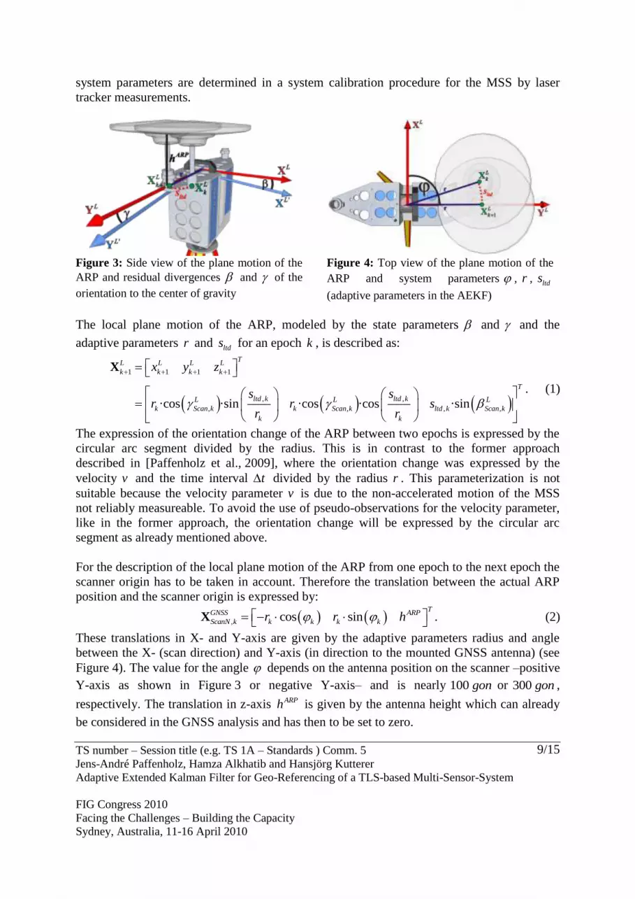
system parameters are determined in a system calibration procedure for the MSS by laser

tracker measurements.

Figure 3: Side view of the plane motion of the

ARP and residual divergences and of the

orientation to the center of gravity

Figure 4: Top view of the plane motion of the

ARP and system parameters , r , ltds

(adaptive parameters in the AEKF)

The local plane motion of the ARP, modeled by the state parameters and and the

adaptive parameters r and ltds for an epoch k , is described as:

1 1 1

,

1

,

, , , ,·cos ·sin ·cos ·cos ·sin

TL L L L

k k k

T

ltd k ltd kL L L

k Scan k k Scan k ltd k Scan k

k k

k x y z

r rr

s ss

r

X

. (1)

The expression of the orientation change of the ARP between two epochs is expressed by the

circular arc segment divided by the radius. This is in contrast to the former approach

described in [Paffenholz et al., 2009], where the orientation change was expressed by the

velocity v and the time interval t divided by the radius r . This parameterization is not

suitable because the velocity parameter v is due to the non-accelerated motion of the MSS

not reliably measureable. To avoid the use of pseudo-observations for the velocity parameter,

like in the former approach, the orientation change will be expressed by the circular arc

segment as already mentioned above.

For the description of the local plane motion of the ARP from one epoch to the next epoch the

scanner origin has to be taken in account. Therefore the translation between the actual ARP

position and the scanner origin is expressed by:

, cos sinGNSS ARP

ScanN k k k k k

T

hr r X . (2)

These translations in X- and Y-axis are given by the adaptive parameters radius and angle

between the X- (scan direction) and Y-axis (in direction to the mounted GNSS antenna) (see

Figure 4). The value for the angle depends on the antenna position on the scanner –positive

Y-axis as shown in Figure 3 or negative Y-axis– and is nearly 100 gon or 300 gon ,

respectively. The translation in z-axis ARPh is given by the antenna height which can already

be considered in the GNSS analysis and has then to be set to zero.




FIG Congress 2010



10/15

To finish the local plane motion description of the ARP, the local orientation , 1

L

Scan k , which

is updated by ,, 1 ,

L L ltd kScan k Scan k

k

s

r , has to be regarded:

1 , 1 ,·L L L GNSS

k ScanN Scan k k ScanN k

L ΔX R X X . (3)

The transformation of the local plane motion given in equation (3) is the last step in modeling

of the motion of the ARP in the local coordinate system besides the consideration of the ARP

position in the epoch k :

1 1( , )· ·G

G

G G G G L

k k L k

X X R R ΔX , (4)

whereby G G

L

R defines the global azimuthal orientation and ( , )G

G

R describes the

transformation from the local to the global coordinate system. The value for the initial global

azimuthal orientation G , the longitude , and latitude of the MSS are calculated as mean

values of all trajectory points.

We can conclude that the state vector kX is given as follows:

, , , , , ,

TTG L L L

g k a k k Scan k Scan k Scank k k k ltd kr s X x x X (5)

with g , kx the general state vector and

a, kx the adaptive state vector.

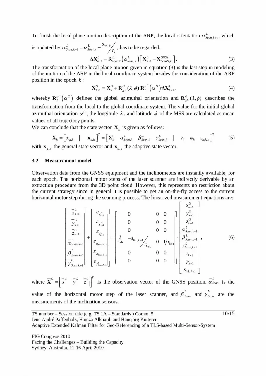
3.2 Measurement model

Observation data from the GNSS equipment and the inclinometers are instantly available, for

each epoch. The horizontal motor steps of the laser scanner are indirectly derivable by an

extraction procedure from the 3D point cloud. However, this represents no restriction about

the current strategy since in general it is possible to get an on-the-fly access to the current

horizontal motor step during the scanning process. The linearized measurement equations are:

1

1

1

, 1

, 1

, 1

, 16 6

1, 11

, 1

, 1

1

1

1

0 0 0

0 0 0

0 0 0

0 1

0 0 0

0 0 0

Gk

Gk

Gk

LScan k

LScan k

LScan k

G

G

G

L ltd

k x

kx

kScan kk

L

Scan k

L

Scan

yk

zk

k

x

y

zI s

rr

1

1

1

, 1

1

, 1

1

1

1

,

,

G

k

G

k

G

k

L

Scan k

L

Scan k

L

Scan k

l d

k

k

t k

x

y

z

r

s

, (6)

where G G G G

T

x y z

X is the observation vector of the GNSS position, L

Scan is the

value of the horizontal motor step of the laser scanner, and L

Scan and L

Scan are the

measurements of the inclination sensors.




FIG Congress 2010



11/15

4. PRACTICAL INVESTIGATIONS OF THE ANEW DEVELOPED ALGORITHM

This section treats the practical investigations of the anew developed algorithm and is

structured into three parts. First, the observations strategy of the practical investigations is

discussed. Second, a brief overview of the GNSS analysis is given. Third, an example dataset

is studied. In contrast to the numerical investigations in [Paffenholz et al., 2009] the results of

the practical measurements with the MSS setup in Figure 1 are discussed here. The

measurements were performed in front of the GIH building using only one fixed station. The

preliminary results of the TLS-based MSS, such as the state parameters, are discussed.

4.1 Observation strategy for the practical investigations

In the present strategy only one GNSS equipment is used to observe the orbital motion of the

MSS. The simultaneously captured data of all sensors, which were already described in

Section 2.3, is the only environment-specific input data for the AEKF. The adaptive

parameters are estimated in a calibration procedure under laboratory conditions with a laser

tracker. The required values for the connection of the local and the global coordinate system

are calculated by the kinematic GNSS observations. For the longitude and latitude this a

feasible solution due to the huge number of 3D positions. The absolute orientation is also

determinable in this way but the reliability of the result is not optimal. One can get results for

a metric uncertainty caused by the global azimuth in a range of a few centimeters in a distance

of about 35 m [Paffenholz & Kutterer, 2008].

In order to improve the result of the global azimuth, a modified observation strategy will be

performed for the upcoming practical investigations. In other words, this means to realize

initialization measurements before the further data acquisition will start, and to use two GNSS

antennas on top of the laser scanner. Within the initialization measurements, rapid-static

GNSS observations should be done only at a minor number of predefined positions. It is

expected to derive a more reliable global azimuth information by these positions.

Another modification of the observation strategy affects the inclination information about the

X- and Y-axis of the MSS. However, it could be an alternative way to get reliable inclinations

to carry out also measurements with the inclinometers at a minor number of predefined

positions. Afterwards a representative function for the inclination plane of the MSS can be

derived, which can be used instead or parallel to the inclinometer measurements during the

scanning process.

4.2 GNSS analysis strategy

The kinematic GNSS analysis strategy depends on the number of used GNSS equipments

(receiver and antenna) in the MSS. Each ARP describes a space curve due to the orbital

motion of the laser scanner. The current setup of the MSS consists of one GNSS equipment

which operates with a data acquisition rate of 10 Hz. If two GNSS equipments are used in the

MSS, the GNSS analysis can be done in two different ways. One way is the calculation of one

single baseline for each equipment. The combination of the two ARP trajectories has then to





FIG Congress 2010



12/15

be realized in the subsequent filter algorithm. The other way is the calculation of a relative

baseline between the two GNSS antennas installed on top of the laser scanner. Within the

filter algorithm there is no combination step necessary. Apart from the 3D positions of the

ARP trajectory the corresponding variance-covariance matrices are regarded within the filter

algorithm to derive the position and especially the orientation of the MSS.

For the kinematic GNSS data processing several approaches are possible. The common

characteristic of all three approaches is the data post-processing. In addition a GNSS

reference station is required to obtain precise 3D positions for the orbital motion of the ARP

as well as for an additional transformation to a global coordinate system. Also a real-time

processing would be possible. The consequence will be higher variances for the 3D positions.

The three post-processing approaches differ with regard to the used GNSS reference station

which could be: a) a commercially running reference station, e.g., of the German reference

station network SAPOS, b) an own temporal reference station positioned on a physical point

with known coordinates nearby the scanning scene, and c) a virtual reference station close to

the scanning scene calculated by at least three reference stations of approach a).

4.2.1 Brief discussion of the error budget of the GNSS component

The 3D positions and their variances are of great importance for the quality of the position

and orientation information of the MSS. On the one hand the error budget of the GNSS

components in combination with the environment has to be considered. These are errors like

near-field effects caused by the antenna adaption made of aluminum on the laser scanner or

possibly multipath effects. Also the data acquisition principle within the MSS has to be

considered with respect to the orbital motion of the laser scanner. This could affect another

error caused by the alternating antenna orientation. Here a solution may be reached by the

introduction of azimuthal dependent phase center variations. On the other hand the kinematic

GNSS data processing itself has an effect on the quality of the 3D positions and on the

derived position and orientation for the MSS.

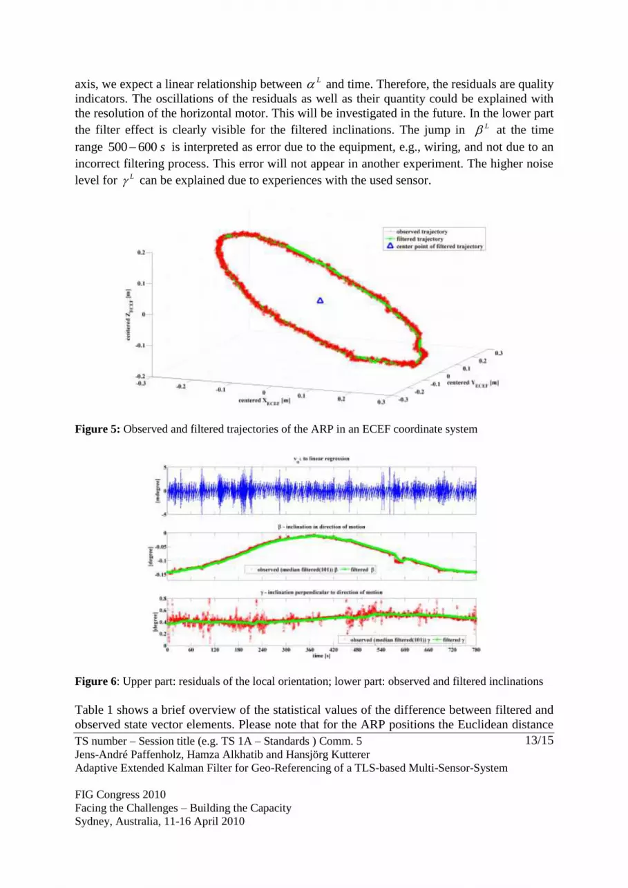
4.3 Example dataset

Figure 5 and Figure 6 present a subsample of the estimated state parameters by the AEKF,

which was discussed in detail in Section 3. The elements of the matrix of process noise in the

AEKF are rather pessimistic values mainly based on experiences with the different sensors

and the first practical datasets. One main topic of the ongoing research work is to get a better

understanding of the process noise and to perform a variance component estimation to

improve the filtering results. For the data acquisition a phase-based laser scanner

Zoller+Fröhlich Imager 5006, one Trimble GPS receiver R5700 with Geodetic Zephyr

antenna and two Schaevitz LSOC-1° inclinometers were used.

In Figure 5 the filter effect is clearly visible for the first three state parameters in an Earth

Centered, Earth Fixed (ECEF) coordinate system. The blue triangle in the middle of the

trajectory represents the center point of the filtered positions or translation vector of the MSS,

respectively. In the upper part of Figure 6 the residuals obtained within a linear regression of

the local orientation L are shown. Due to the constant rotation of the TLS about its vertical




FIG Congress 2010



13/15

axis, we expect a linear relationship between L and time. Therefore, the residuals are quality

indicators. The oscillations of the residuals as well as their quantity could be explained with

the resolution of the horizontal motor. This will be investigated in the future. In the lower part

the filter effect is clearly visible for the filtered inclinations. The jump in L at the time

range 500 600 s is interpreted as error due to the equipment, e.g., wiring, and not due to an

incorrect filtering process. This error will not appear in another experiment. The higher noise

level for L can be explained due to experiences with the used sensor.

Figure 5: Observed and filtered trajectories of the ARP in an ECEF coordinate system

Figure 6: Upper part: residuals of the local orientation; lower part: observed and filtered inclinations

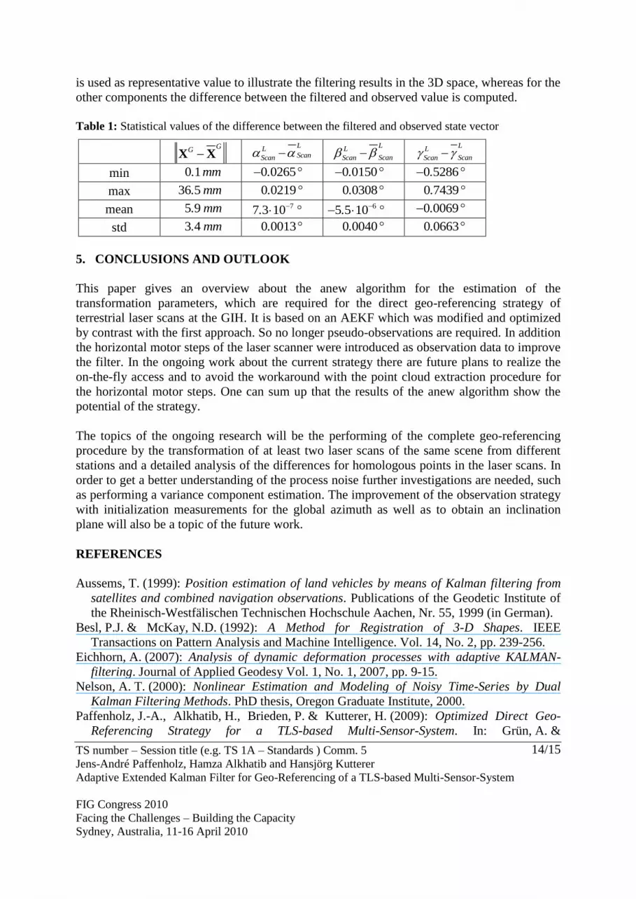
Table 1 shows a brief overview of the statistical values of the difference between filtered and

observed state vector elements. Please note that for the ARP positions the Euclidean distance




FIG Congress 2010



14/15

is used as representative value to illustrate the filtering results in the 3D space, whereas for the

other components the difference between the filtered and observed value is computed.

Table 1: Statistical values of the difference between the filtered and observed state vector

GG X X

LLScanScan

LL

ScanScan L

L

ScanScan

min 0 1. mm 0 0265. 0 0150. 0 5286.

max 36 5. mm 0 0219. 0 0308. 0 7439.

mean 5 9. mm 77 3 10. 65 5 10.

0 0069.

std 3 4. mm 0 0013. 0 0040. 0 0663.

5. CONCLUSIONS AND OUTLOOK

This paper gives an overview about the anew algorithm for the estimation of the

transformation parameters, which are required for the direct geo-referencing strategy of

terrestrial laser scans at the GIH. It is based on an AEKF which was modified and optimized

by contrast with the first approach. So no longer pseudo-observations are required. In addition

the horizontal motor steps of the laser scanner were introduced as observation data to improve

the filter. In the ongoing work about the current strategy there are future plans to realize the

on-the-fly access and to avoid the workaround with the point cloud extraction procedure for

the horizontal motor steps. One can sum up that the results of the anew algorithm show the

potential of the strategy.

The topics of the ongoing research will be the performing of the complete geo-referencing

procedure by the transformation of at least two laser scans of the same scene from different

stations and a detailed analysis of the differences for homologous points in the laser scans. In

order to get a better understanding of the process noise further investigations are needed, such

as performing a variance component estimation. The improvement of the observation strategy

with initialization measurements for the global azimuth as well as to obtain an inclination

plane will also be a topic of the future work.

REFERENCES

Aussems, T. (1999): Position estimation of land vehicles by means of Kalman filtering from

satellites and combined navigation observations. Publications of the Geodetic Institute of

the Rheinisch-Westfälischen Technischen Hochschule Aachen, Nr. 55, 1999 (in German).

Besl, P.J. & McKay, N.D. (1992): A Method for Registration of 3-D Shapes. IEEE

Transactions on Pattern Analysis and Machine Intelligence. Vol. 14, No. 2, pp. 239-256.

Eichhorn, A. (2007): Analysis of dynamic deformation processes with adaptive KALMAN-

filtering. Journal of Applied Geodesy Vol. 1, No. 1, 2007, pp. 9-15.

Nelson, A. T. (2000): Nonlinear Estimation and Modeling of Noisy Time-Series by Dual

Kalman Filtering Methods. PhD thesis, Oregon Graduate Institute, 2000.

Paffenholz, J.-A., Alkhatib, H., Brieden, P. & Kutterer, H. (2009): Optimized Direct Geo-

Referencing Strategy for a TLS-based Multi-Sensor-System. In: Grün, A. &










FIG Congress 2010



15/15

Kahmen, H. (Eds.): Optical 3D-Measurement Techniques IX, Vol. I, Vienna, Austria,

2009, pp. 287-292.

Paffenholz, J.-A. & Kutterer, H. (2008): Direct Georeferencing of Static Terrestrial Laser

Scans. FIG Working Week 2008, Stockholm, Sweden, June 14-19 2008.

Simon, D. (2006): Optimal State Estimation. Wiley, Hoboken, New Jersey, 2006.

Vennegeerts, H., Martin, J., Becker, M. & Kutterer, H. (2008): Validation of a kinematic

laserscanning system. Journal of Applied Geodesy, Vol. 2, No. 2, pp. 79-84.

BIOGRAPHICAL NOTES

Jens-André Paffenholz received his Dipl.-Ing. in Geodesy and Geoinformatics at the Leibniz

Universität Hannover. Since 2006 he has been research assistant at the Geodetic Institute at

the Leibniz Universität Hannover. His main research interests are: terrestrial laser scanning,

industrial measurement systems, and process automation of measurement systems. He is

active in the Working Group 4.2.3 “Application of Artificial Intelligence in Engineering

Geodesy” of the IAG Commission 4 (Positioning and Applications).

Dr. Hamza Alkhatib received his Dipl.-Ing. in Geodesy and Geoinformatics at the

University of Karlsruhe in 2001 and his Ph.D. in Geodesy and Geoinformatics at the

University of Bonn in 2007. Since 2007 he has been postdoctoral fellow at the Geodetic

Institute at the Leibniz Universität Hannover. His main research interests are: Bayesian

Statistics, Monte Carlo Simulation, Modeling of Measurement Uncertainty, Filtering and

Prediction in State Space Models, and Gravity Field Recovery via Satellite Geodesy.

Prof. Dr. Hansjörg Kutterer received his Dipl.-Ing. and Ph.D. in Geodesy at the University

of Karlsruhe in 1990 and 1993, respectively. Since 2004 he has been a Full Professor at the

Geodetic Institute of the Leibniz Universität Hannover. His research areas are: adjustment

theory and error models, quality assessment, geodetic monitoring, terrestrial laser scanning,

multi sensor systems, and automation of measurement processes. He is active in national and

international scientific associations. In 2009 he became a Vice President of the DVW –

Gesellschaft für Geodäsie, Geoinformatik und Landmanagement. In addition he is member of

the editorial boards of three scientific journals.

CONTACTS

Jens-André Paffenholz Dr. Hamza Alkhatib

Tel. +49 511 762 3191 Tel. +49 511 762 2464

Email: [email protected] Email: [email protected]

Prof. Dr. Hansjörg Kutterer Geodätisches Institut

Tel. +49 511 762 2461 Leibniz Universität Hannover

Email: [email protected] Nienburger Str. 1

30167 Hannover

GERMANY

Webpage: www.gih.uni-hannover.de





Documents

Adaptive extended Kalman filter for geo-referencing of a TLS-based multi-sensor-system