Embed Size (px)
Citation preview
Hindawi Publishing CorporationMathematical Problems in EngineeringVolume 2013 Article ID 609523 12 pageshttpdxdoiorg1011552013609523
Research ArticleActive Disturbance Rejection Approach forRobust Fault-Tolerant Control via Observer AssistedSliding Mode Control
John Corteacutes-Romero1 Harvey Rojas-Cubides1 Horacio Coral-Enriquez1
Hebertt Sira-Ramiacuterez2 and Alberto Luviano-Juaacuterez3
1 Departamento de Ingenierıa Electrica y Electronica Universidad Nacional de Colombia Carrera 45 No 26-85 Bogota Colombia2 Centro de Investigacion y de Estudios Avanzados del Instituto Politecnico Nacional (CINVESTAV-IPN)Avenida Instituto Politecnico Nacional No 2508 Departamento de Ingenierıa Electrica Seccion de MecatronicaColonia San Pedro Zacatenco AP 14740 07300 Mexico DF Mexico
3 Unidad Profesional Interdisciplinaria en Ingenierıa y Tecnologıas Avanzadas (UPIITA) Instituto Politecnico NacionalAvenida Instituto Politecnico Nacional 2580 Barrio La Laguna Ticoman Gustavo A Madero 07340 Mexico DF Mexico
Correspondence should be addressed to John Cortes-Romero jacortesrunaleduco
Received 23 August 2013 Revised 4 November 2013 Accepted 6 November 2013
Academic Editor Baoyong Zhang
Copyright copy 2013 John Cortes-Romero et al This is an open access article distributed under the Creative Commons AttributionLicense which permits unrestricted use distribution and reproduction in any medium provided the original work is properlycited
This work proposes an active disturbance rejection approach for the establishment of a sliding mode control strategy in fault-tolerant operations The core of the proposed active disturbance rejection assistance is a Generalized Proportional Integral (GPI)observer which is in charge of the active estimation of lumped nonlinear endogenous and exogenous disturbance inputs related tothe creation of local sliding regimes with limited control authority Possibilities are explored for the GPI observer assisted slidingmode control in fault-tolerant schemes Convincing improvements are presented with respect to classical sliding mode controlstrategies As a collateral advantage the observer-based control architecture offers the possibility of chattering reduction given thata significant part of the control signal is of the continuous type The case study considers a classical DC motor control affected byactuator faults parametric failures and perturbations Experimental results and comparisons with other established sliding modecontroller design methodologies which validate the proposed approach are provided
1 Introduction
Themain challenge of the Fault-TolerantControl is to guaran-tee high performance and reliability in themost adverse oper-ations such as the presence of perturbations disturbancesdynamic miss-modeling and actuator faults among othersIn general the techniques employed on the Fault-tolerantControl (FTC) can be classified into active and passiveActive FTC is characterized by the controller reconfigurationassisted by fault detection and isolation (FDI) schemes [1] Onthe other hand passive techniques exploit the robustness ofsome types of controllers without requiring changes in theirstructure and can operate satisfactorily without informationabout system failures These techniques are usually simple
in implementation but are not usually suitable for severe casesof failures [1]
The robust characteristics of the sliding mode techniqueprovide a natural environment for the use of such techniqueson passive FTC schemes This technique has been properlyused in different control schemes and assisted by other effec-tive control strategies which have shown proper performanceunder fault-tolerant operations (see [1ndash4] as representativeexamples) Over the past years considerable attention hasbeen paid to the design of linearnonlinear disturbanceobservers for sliding mode controller assistance in order toovercome several issues like chattering [5ndash8] disturbancesand system uncertainties [8ndash10] coupling of MIMO systems[11] or uncertainties disturbances and actuator faults [12]
2 Mathematical Problems in Engineering
Even though the performance of the aforementionedcontrol proposals is accurate there are still complexities inthe design that are a consequence of dealing with the systemfaults and disturbances separately on the one hand and onthe other hand the need for precise knowledge of the systemmodel
In the active disturbance rejection control (ADRC) phi-losophy system fault and disturbances can be dealt withunitedly rendering a simplified linear control structure basedon a simplified model like the classical passive fault-tolerantscheme From the ADRC point of view the disturbancesmust be rejected in an active manner so the control systemactively produces accurate estimates and reduces the causesof the output errors ADRC as a potential solution has beenexplored in several domains of control engineering (see [13ndash15]) In accordance with this field Generalized ProportionalIntegral (GPI) observers were introduced in [16] Despiteof grand ADRC applications reported in the literature thepotential of this technique for fault-tolerant performance hasbeen scarcely considered Under the ADRC setup a GPI dis-turbance observer assisted slidingmode control approach canbe used to deal with fault-tolerant operation In this paper thelinear GPI observers are used as a part of an active distur-bance rejection scheme for the slidingmode creation problemon nonlinear systems with low switching authority
We are interested in a proper local sliding mode creationwith the aid of a GPI disturbance observer In the establish-ment of the slide surface unknown inputs (state dependentor external) impact the correct evolution of the slidingregime demanding greater bound of the control input whenthe sliding surface dynamics include an active disturbancecancellation of the influence of that kind of unknown inputsthe required switching input amplitude can be decreasedFurthermore risk for deviations from the sliding surfacedue to unexpected control input saturations is practicallyavoided The proposed GPI observer can be related to eitherthe system dynamics or sliding surface dynamics disturbanceinputs in both cases it is possible to correctly design asuitable assisted sliding mode control law with fault-tolerantcapabilities
It is assumed that the effect of additive state-dependentand exogenous nonlinearities that affect the sliding moderegime may be approximately but accurately canceled fromthe nonlinear system behavior via the injection of a preciseand exogenously generated time-varying signal
In this work we propose an approach of passive fault-tolerant control based on a classic sliding mode controllerassisted by a GPI observer under the context of the activedisturbance rejection This scheme has been validated withthe control of a DCmotor subject to perturbations in the loadtorque actuator faults and parametric failures
This paper is organized as follows Section 2 exploresthe possibilities of the ADRC in GPI based observer slidingmode control for fault-tolerant operation and two relateduseful cases are presented Section 3 describes the studycase states the formulation of the problem and presents itscorresponding proposed design Section 4 is devoted to thepresentation of the experimental results describing experi-mental platform and the experiments that were carried out
to enhance the advantages of using the linear estimation ofthe disturbance functions during the sliding mode creationproblem Finally Section 5 contains the conclusions
2 Possibilities of ADRC for Sliding ModeControl Assistance
It is possible to assist the creation of a slidingmode regime fora wide variety of sliding mode control strategies The idea isto inject a continuous term via a suitably defined observer inan active fashion at the controller stage to ensure the correctestablishment or continuation of the sliding mode regime
The objective of the proposed fault-tolerant controldesign is to accurately track a desired reference trajectoryeven in the presence of the unknown disturbances causedby actuator faults parameter uncertainty the presence ofunmodeled state-dependent nonlinearities or the combina-tion of these previous cases with the presence of uncertainexogenous time-varying signals
This is explained in this section by using a GPI observer-based sliding mode controller From this point of view allthose terms are considered as a single lumped unstructuredtime-varying disturbance term In the establishment of theslidingmode control law it is necessary to have an estimationof the related disturbance term Two main benefits of usingthis strategy can be highlighted (1) GPI observers allow theestimation of the state of the system the related disturbancefunction and a certain number of its time derivatives (2)the control law is composed of a discontinuous term plusa continuous injection provided by the GPI observer Theamplitude of the switching part (119882) acts as a weighting factorallowing the chattering reduction
In the following section two approaches for the creationof the sliding mode regimes assisted by GPI observerssuitable for fault-tolerant operation are explained
It should be noted that our approach is not the onlypossibility it is merely a preferred approach with ease ofanalysis (eg it is possible to propose a GPI observer assistedstrategy of high-order sliding mode)
21 On Observer Assisted First Order Sliding Mode CreationIn this subsection a conventional first order sliding modecontrol is appropriately adapted by a GPI observer Considerthe following 119899-dimensional nonlinear single-input single-output system
= 119891 (119909) + 119892 (119909) 119906 120590 = ℎ (119909) (1)
where the drift vector field 119891(119909) is a smooth but uncertainvector field on 119879R119899 119892(119909) is known and a smooth vectorfield on 119879R119899 and 119906 is the control input taking values on theclosed interval [minus119880119880]119880 gt 0 The function ℎ(119909) is a smoothfunction ℎ R119899 rarr R The zero level set for the scalar output120590
119878 = 119909 isin R119899
| 120590 = ℎ (119909) = 0 (2)
represents a smooth 119899 minus 1 dimensional manifold acting asa sliding surface where 120590 is the sliding surface coordinatefunction
Mathematical Problems in Engineering 3
The state-dependent unperturbed sliding surface dynam-ics are characterized by
= 119871119891ℎ (119909) + 119871
119892ℎ (119909) 119906 (3)
where 119871119891and 119871
119892are the Lie derivatives or the directional
derivatives of ℎ along the directions of the vectors 119891 and 119892respectively
Actuator faults exogenous disturbances modeled andnon modeled internal dynamics and possible parametervariation can be treated as an equivalent additive lumped dis-turbance function 120585
120590 affecting the sliding surface dynamic120590
= 120585120590+ 119871119892ℎ (119909) 119906 (4)
211 Assumptions
Assumption 1 The amplitude119882 of the switching part of thecontrol input 119906 satisfies119882 lt 119880
Assumption 2 The disturbance function 120585120590 and a finite
number of its time derivatives 120585(119896)120590 119896 = 0 1 2 119898 for a
sufficiently large 119898 are assumed to be uniformly and abso-lutely bounded that is 0 le |120585(119896)
120590| le 120575119896lt infin for any feedback
control input stabilizing the sliding surface coordinatedynamics
Assumption 3 Weassume that119871119892ℎ(119909) gt 0 is perfectly known
and locally strictly positiveThe key observation for the robust operation of the
proposed sliding regimes is based on the accurate yetapproximate on-line estimation of the scalar uncertain dis-turbance function 120585
120590in the form 120585
120590 The incorporation of
that estimation in the slidingmode control lawmay result in asubstantially enhanced possibility for the creation of a slidingmotion via the active disturbance cancelation strategy
119906 =1
119871119892ℎ (119909)
[minus120585120590minus119882 sign (120590)] (5)
An extended state representation can be proposed tocope with the disturbance function estimation 120585
120590 The aug-
mented representation is based on the internal model ofthe disturbance function 120585
120590 When there is no previous
knowledge about the disturbance term 120585120590 a general signal
oriented approach can be quite effective for on-line estima-tion purposes Associated with ADRC and specialized byGPIapproaches unknown input signals can be approximated by119889119898
120585120590119889119905119898
asymp 0 For that realization the extended state vector119909120590= [120590 120585
120590120585(1)
120590sdot sdot sdot 120585(119898minus1)
120590]119879
is considered Therefore theextended state space representation is given by
120590= 1198601119909120590+ 119861120590119871119892ℎ (119909) 119906 + 119864
120590120585(119898)
(6)
where
1198601=
[[[[[[
[
0 1 0 sdot sdot sdot 0
0 0 1 0
d
0 0 0 sdot sdot sdot 1
0 0 0 sdot sdot sdot 0
]]]]]]
]
119861120590=
[[[[[[
[
1
0
0
0
]]]]]]
]
119864120590=
[[[[[[
[
0
0
0
1
]]]]]]
]
(7)
The disturbance function estimation is given by thefollowing GPI observer
Theorem 1 Letting 119911 = [11991111199112sdot sdot sdot 119911119898+1]119879 and Γ =
[120574119898120574119898minus1
sdot sdot sdot 1205740]119879 with Assumptions 1ndash3 the following
observer for system (4) = 119860
1119911 + 119861120590119871119892ℎ (119909) 119906 + Γ119890
120590(8)
with119898 being a sufficiently large integer produces exponentiallyasymptotic estimation of 120590 120585
120590 120585
(119898minus1)
120590given by the observer
variables 1199111 1199112 119911
119898 respectively The estimation errors (120590minus
1199111) (120585120590minus 1199112) (120585
(119898minus1)
120590minus 119911119898+1) are ultimately uniformly
bounded given the design parameters 1205740 120574
119898that are chosen
so that the following characteristic polynomial is Hurwitz
119901119890120590
(119904) = 119904119898+1
+ 120574119898119904119898
+ sdot sdot sdot + 1205741119904 + 1205740 (9)
Proof The corresponding estimation error vector is definedas 119890120590= 119909120590minus 119911 and satisfies
119890120590= (1198601minus 119871119862) 119890
120590+ 119864120590120585(119898)
= 119860120590119890120590+ 119864120590120585(119898)
(10)
with
119860120590=
[[[[[[
[
minus120574119898
1 0 sdot sdot sdot 0
minus120574119898minus1
0 1 0
dminus1205741
0 0 sdot sdot sdot 1
minus1205740
0 0 sdot sdot sdot 0
]]]]]]
]
isin R(1+119898)times(1+119898)
(11)
and its characteristic polynomial in the complex variable 119904 isgiven by
119901119890120590
(119904) = det (119904119868 minus 119860120590) = 119904119898+1
+ 120574119898119904119898
+ sdot sdot sdot + 1205741119904 + 1205740 (12)
where the eigenvalues of 119860120590can be placed as desired by
selecting the gain vector Γ The Hurwitzian character of 119860120590
implies that for every constant (1+119898)times (119899+119898) symmetricpositive definitematrix119876 = 119876119879 gt 0 there exists a symmetricpositive definite (1 +119898) times (1 +119898)matrix 119875 = 119875119879 gt 0 so that119860119879
120590119875 + 119875119860
120590= minus119876 The Lyapunov function candidate 119881(119909) =
(12)119890119879
120590119875119890120590exhibits a time derivative alongwith the solutions
of the closed loop system given by
(119890120590 119905) =
1
2119890119879
120590(119860119879
120590119875 + 119875119860
120590) 119890120590+ 119890119879
120590119875119864120590120585(119898)
120590(119905) (13)
For 119876 = 119868 that is an (1 + 119898) times (1 + 119898) identity matrix thisfunction satisfies
(119909120590 119905) =
1
2119890119879
120590(minus119876) 119890
120590+ 119890119879
120590119875119864120590120585(119898)
120590(119905)
le1
2
10038171003817100381710038171198901205901003817100381710038171003817
2
2+10038171003817100381710038171198901205901003817100381710038171003817211987521198642120575119898
(14)
4 Mathematical Problems in Engineering
Given that 1198642= 1 and according to Assumption 2 this
function is strictly negative everywhere outside the sphere 119878120590
given by
119878120590= 119890120590isin 1198771+119898
|100381710038171003817100381711989012059010038171003817100381710038172le 21205751198981198752 (15)
Hence all trajectories 119890120590(119905) starting outside this sphere
converge towards its interior and all those trajectories start-ing inside 119878
120590will never abandon it
Corollary 2 Under all the previous assumptions the discon-tinuous active disturbance rejection feedback controller
119906 =1
119871119892ℎ (119909)
[minus1199111minus119882 sign (120590)] (16)
locally creates a sliding regime for any amplitude119882 satisfying119882 gt 120575
0 with 120575
0as the ultimate bound for the disturbance
estimation error 119890120590
Proof The observer-based control law renders the followingclosed loop sliding surface dynamics
= (120585120590minus 120585120590) minus119882 sign (120590) (17)
with 120585120590= 1199111 which would require a smaller control input
switching amplitude119882 than in the case where the observer isnot used According toTheorem 1 the disturbance estimationerror 119890
120590 is bounded by 120575
1 and the local existence of a sliding
regime 120590 = 0 is guaranteed even if119882 is rather smallConsider the following Lyapunov function candidate
119881 =1
21205902
(18)
Differentiating the Lyapunov function (18) with respect totime and using (17) yield
= 120590
= 120590 (120585120590minus 120585120590minus119882 sign (120590))
= 120590 (120585120590minus 120585120590) minus119882 |120590|
le |120590| 1205750minus119882 |120590|
(19)
is strictly negative if119882 gt 1205750 Therefore if119882 gt 120575
0 locally
it creates a sliding regime (see [17])
22 Observer Assisted Nonlinear Controlled Systems in Input-Output Representation In the previous subsection the powerof the GPI observer injections for a proper establishmentand development of a first order sliding mode regimen wasdemonstrated In this subsection the GPI observer is used ina wider perspective allowing both sliding surface coordinatefunction (120590) and disturbance function (120585
120590) constructions
These constructions are conducted by means of the systemstate estimation and disturbance function estimation relatedto system dynamics all are supplied by the GPI observer
Consider the nonlinear scalar differentially flat system
119910(119899)
= 120595 (119905 119910) 119906 + 120601 (119905 119910 119910 119910(119899minus1)
) (20)
with the following set of initial conditions 1198840= 119910(119905
0)
119910(1199050) 119910
(119899minus1)
(1199050) We refer to the function 120595(119905 119910) as the
control input gain of the system The term 120601(119905 119910 119910
119910(119899minus1)
) will be addressed as the drift functionFor a given smooth control input function 119906(119905) let 119910(119905) =
Θ(119905 1199050 1198840 119906(119905)) denote the solution trajectory of system (20)
from the set of initial conditions 1198840 We denote by the time
function 120585(119905) the additive disturbance function regardless ofany particular internal structure
It is desired to drive the flat output 119910 of the system
119910(119899)
= 120595 (119905 119910) 119906 + 120585 (119905) (21)
to track a given smooth reference trajectory 119910lowast(119905) regardlessof the unknown but uniformly bounded nature of thedisturbance function 120585(119905) As in the previous case 120585 takesinto account in a lumped way faults and exogenous andendogenous disturbances affecting the system dynamics Itis important to note that the disturbance functions 120585 and 120585
120590
are defined in different dynamics but catch the same essentialdisturbance behavior Indeed it will be showed that it ispossible to form an estimate of 120585
120590from an estimate of 120585 and
some others estimates provided by the GPI observerRegarding controlled system (21) we make the following
assumptions
Assumption 4 The disturbance function 120585(119905) is completelyunknown while the control input gain 120595(119905 119910) is perfectlyknown Let 120598 be a strictly positive real number The controlinput gain 120595(119905 119910) is assumed to be uniformly bounded awayfrom zero that is inf
119905|120595(119905 119910)| ge 120598 gt 0 for any solution 119910(119905) of
the controlled system In particular it is bounded away fromzero for the given output reference trajectory 119910lowast(119905)
Assumption 5 It is assumed that a solution 119910(119905) existsuniformly in 119905 for every given set of initial conditions 119884
0
specified at time 119905 = 1199050and for a given sufficiently smooth
control input function 119906(119905) Given a desired flat outputreference trajectory 119910lowast(119905) the flatness of the system and theprevious assumption a straightforward calculation of the cor-responding (unique) open loop control input 119906lowast(119905) is possible(see [18])
Assumption 6 Let 119898 be a given integer As a time functionthe 119898th time derivative of 120585(119905) is uniformly absolutelybounded In other words there exists a constant119870
119898so that
sup119905
10038161003816100381610038161003816120585(119898)
(119905)10038161003816100381610038161003816le 119870119898 (22)
Remark 3 Assumption 6 cannot be verified a priori when120585(119905) is completely unknown However in cases where thenonlinearity is known except for some of its parameters itsvalidity can be assessed with some work Also if 120585(119898)(119905) isnot uniformly absolutely bounded almost everywhere thensolutions 119910(119905) for (21) do not exist for any finite 119906(119905) (see [19])
Mathematical Problems in Engineering 5
221 Observer-Based Approach With reference to simplifiedsystem (21) in order to propose a GPI observer for a relatedstate and disturbance function estimation it is consideredthat the internal model of the disturbance function 120585 isapproximated by 119889119898120585(119905)119889119905119898 asymp 0 at the observer stageThismodel is embedded into the augmentedmodel which is char-acterized by an extended state composed of the phase vari-ables119909
1 1199092 119909
119899 associatedwith the flat output119909
1= 119910 and
augmented by the119898 output estimation error iterated integralinjections 119909
119899+1 119909
119899+119898 As a result setting the state vector
119909 = [11990911199092sdot sdot sdot 119909
119899+119898] with 119909
1= 119910 119909
2= 119910 119909
119899= 119910(119899minus1)
119909119899+1
= 120585 119909119899+119898
= 120585(119898minus1) the augmented state spacemodel
is given by
= 119860119909 + 119861120595 (119905 119910) 119906 + 119864120585(119898)
119910 = 119862119909
(23)
with
119860 =
[[[[[[
[
0 1 0 sdot sdot sdot 0
0 0 1 0
d0 0 0 sdot sdot sdot 1
0 0 0 sdot sdot sdot 0
]]]]]]
]
isin R(119899+119898)times(119899+119898)
119861 =
[[[[[[[
[
0
1(119899th position)
0
]]]]]]]
]
isin R(119899+119898)times1
119862 = [1 0 sdot sdot sdot 0] isin R1times(119899+119898)
119864 =
[[[[[[
[
0
0
0
1
]]]]]]
]
isin R(119899+119898)times1
(24)
Now the GPI observer for the state 119909 is proposed
119909 = 119860119909 + 119861120595 (119905 119910) 119906 + 119871 (119910 minus 119910)
119910 = 119862119909
(25)
where 119909 = [11990911199092
sdot sdot sdot 119909119899+119898]119879 is the estimation
state vector and the observer gain vector is 119871 =
[119897119899+119898minus1
sdot sdot sdot 11989711198970]119879
The estimation error vector 119890119909= [11989011990911198901199092sdot sdot sdot 119890119909(119899+119898)
]119879
defined as 119890119909= 119909 minus 119909 satisfies
119890119909= (119860 minus 119871119862) 119890
119909+ 119864120585(119898)
119890119909= 119860119890119890119909+ 119864120585(119898)
(26)
where
119860119890=
[[[[[[
[
minus119897119899+119898minus1
1 0 sdot sdot sdot 0
minus119897119899+119898minus2
0 1 0
dminus1198971
0 0 sdot sdot sdot 1
minus1198970
0 0 sdot sdot sdot 0
]]]]]]
]
(27)
with 119860119890isin R(119899+119898)times(119899+119898) and its characteristic polynomial in
the complex variable 119904 is given by
119901119890119909
(119904) = det (119904119868 minus 119860119890)
= 119904119899+119898
+ 119897119899+119898minus1
119904119899+119898minus1
+ sdot sdot sdot + 1198971119904 + 1198970
(28)
Theorem 4 Suppose that all previous assumptions are validLet the coefficients 119897
119895 with 119895 = 0 1 119899 + 119898 minus 1 of the
polynomial 119901119890119909
(119904) be chosen so that all their roots are exhibitedto the left of the complex plane C Then the trajectories of theestimation error vector 119890
119909(119905) globally converge towards a small
as-desired sphere of radius 120588 denoted by 119878(0 120588) centered at theorigin of the estimation error phase space 119890
1199091 1198901199092 119890
119909(119899+119898)
where they remain ultimately bounded
Proof This problem has already been proposed with slightlydifferent notation in [20] In a recent work [21] it is shownthat the estimation error vector is uniformly ultimatelybounded
Remark 5 Consequently with Theorem 4 the variables119909119899+1 119909119899+2 119909
119899+119898track arbitrarily and closely the unknown
time functions 120585(119905) and their time derivatives 120585(119895)(119905) 119895 =
1 119898 minus 1
222 Sliding Surface Design Regarding controlled systems(21) a conventional sliding surface can be chosen as (in orderto decrease the stable error an integral term of the trackingerror 119890
119910can be introduced (see [12]) but it is preferred to
maintain a conventional surface to enhance the GPI observercapabilities)
120590 = 119890(119899minus1)
119910+ 120582119899minus2119890(119899minus2)
119910+ sdot sdot sdot + 120582
0119890119910
(29)
with 119890119910= 119910 minus 119910
lowast being flat output tracking error The designparameters 120582
0 120582
119899minus2are chosen so that the characteristic
polynomial 119901120590(119904) = 119904
(119899minus1)
+ 120582119899minus2119904(119899minus2)
+ sdot sdot sdot + 1205820is Hurwitz
An estimated version of the previous surface can be givenby
= 119909119899minus [119910lowast
](119899minus1)
+ 120582119899minus2(119909119899minus1minus [119910lowast
](119899minus2)
)
+ sdot sdot sdot + 1205820(1199091minus 119910lowast
)
(30)
where 119910 = 1199091
119910(119899minus1) = 119909
119899are estimates provided by
GPI observer (8) The use of 1199091instead of 119909
1is preferred for
chattering reduction purposes (see [17])The sliding surface dynamics of is given by
120590 = 119909119899minus [119910lowast
](119899)
+ 120582119899minus2( 119909119899minus1minus [119910lowast
](119899minus1)
)
+ sdot sdot sdot + 1205820( 1199091minus 119910lowast
)
(31)
6 Mathematical Problems in Engineering
120579 120596
Host PC
Target PC with DAQ boards
MATLABSimulink
Perturbationgenerator Current
control
Fault profilegenerator
control
Signalconditioning
Periodmeasurement
PWMDirection
Analog input
DODO
PWMDirection
(A) signal
DC power supply30Vdc
Full-bridgedriver
Load-motor
Optocouplerrelay circuit
Load-motorshaft shaft
Coupling
Currentsensor
DC-bus level shift fault
DC power supply30Vdc 20Vdc
Faultoff
Faulton
Faultoff
Faulton
Full-bridgedriver
Main-
Main-motor
motor
Coupling
Rotaryencoder
(A B)
Parametric fault
Raf
ilowast(t)
i(t)
lowast(t)
lowast(t)
120596lowast(t)
120596(t)
Speed
Digital outputDigital output
+ +minus minus
Figure 1 General scheme of the experimental setup
On the other hand from the GPI Observer we have
119909119899= 120595 (119905 119910) 119906 + 119909
119899+1+ 119897119898(1199091minus 1199091) (32)
therefore
120590 = 120595 (119905 119910) 119906 + 120585120590
(33)
with
120585120590= 119909119899+1+ 119897119898(1199091minus 1199091) minus [119910
lowast
](119899)
+ 120582119899minus2( 119909119899minus1minus [119910lowast
](119899minus1)
) + sdot sdot sdot + 1205820( 1199091minus [119910lowast
](1)
)
(34)
where the estimates 119909119899minus1 119909
1are also provided by the GPI
observer Remember that as stated by the GPI observer statenotation 119909
119899+1= 120585 as announced at the beginning of this
subsection the disturbance function estimation related tosliding regime (33) 120585
120590is given in terms of 120585 which is related
to system dynamics (21)According to (5) the control law is
119906 =1
120595 (119905 119910)[minus120585120590minus119882 sign ()] (35)
Now consider the following Lyapunov function candi-date
1198811=1
22
(36)
Differentiating the Lyapunov function (36) with respectto time and using (33) and (35) we obtained
1= 120590 = (120595 (119905 119910) 119906 + 120585
120590) = minus119882 || (37)
which assures the sliding mode regime provided that119882 gt 0
3 Case Study
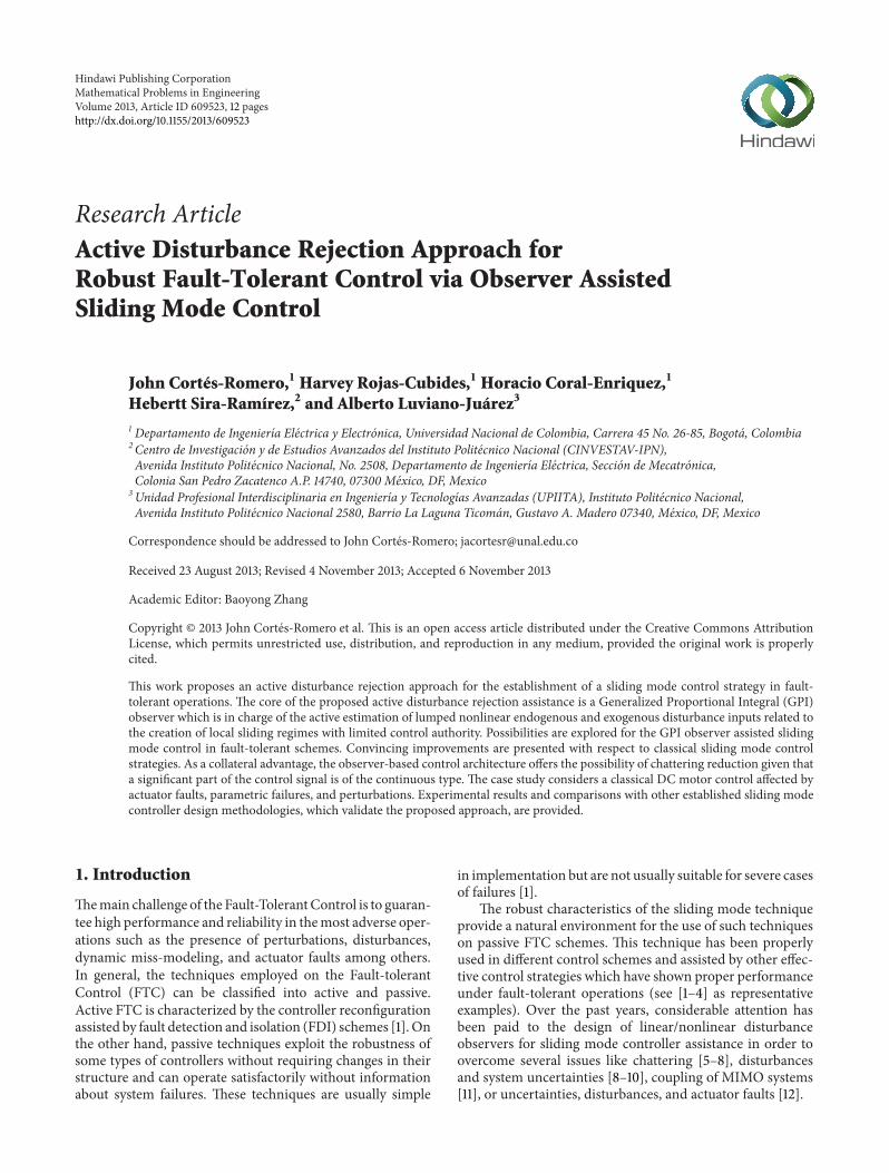
The system used for the experimental comparison of the pro-posed control strategies is a mechatronic system composedof two directly coupled DC motors The first motor (alsocalled the main-motor) acts as the system to be controlledThe second motor (also called the load-motor) generatesperturbation loads to the main-motor Hence the proposedcontrol strategies are applied to control the angular speed ofthemain-motor while the load-motor acts as the load-torqueperturbation generator by means of a current control loopFigure 1 shows a detailed scheme of the mechatronic systemcontrol loops and the experimental setup This figure alsoshows the implementation scheme of two faults armatureresistance fault (fault 1) and DC-bus level shift fault (fault 2)These faults are typical in systems as the one under study (asit will be explained later) and all controllers will be assessedunder these faults
31 Fault-Tolerant Control for DCMotors Themost commonfaults in DC-motor drives can be classified as actuatorparametric and sensor faults [22] The actuator faults aremainly due to the reduction in the performance of amplifiers
Mathematical Problems in Engineering 7
malfunction of power semiconductors and failures in regu-latory stages in the power supply [23 24] Parametric faultsare caused by degradation of brushes inertia and frictionchanges and variations in resistance or inductance of thearmature [22] This paper will consider two faults in themechatronic system
(1) parametric fault due to a change in the resistance ofDC-motor armature and
(2) actuator fault due to level shift of the DC-bus voltagethat feeds the full-bridge drive of the main-motor
32 Problem Formulation Consider the following dynamicmodel describing aDC-motor controlled by armature voltage119906(119905) with state variables given by 120596(119905) describing the rotorangular speed and 119894(119905) representing the armature current
119871119886
119889119894 (119905)
119889119905= 119896pwm119906 (119905) minus 119877119886119894 (119905) minus 119870119887120596 (119905)
119869119898
119889120596 (119905)
119889119905= 119870119879119894 (119905) minus 120591
119871(119905) minus 119861120596 (119905) minus 120575 (120596 (119905))
(38)
The parameters 119871119886and 119877
119886represent the armature induc-
tance and armature resistance 119869119898is the moment of inertia
119870119887is the back-emf constant 119870
119879is the torque constant 119861 is
the viscous friction coefficient 119896pwm is the conversion gain ofPWM 120591
119871represents the unknown load-torque perturbation
input 119906(119905) is the control signal and 120575(120596(119905)) represents anonlinear model of dry friction where119879
119888119879119904 and 120572 are terms
associated with coulomb friction (see [25]) Consider
120575 (120596) = 120596 [gt 119879119888sign (120596) + (119879
119904minus 119879119888) 119890minus120572|120596| sign (120596)]
(39)
By rewriting and lumping together some terms of (38)the following representation of the system (typical of theADRC paradigm) is obtained
(119905) = 120581119906 (119905) + 120585 (119905) (40)
where
120581 =
119870119879119896pwm
119869119898119871119886
120585 (119905) =119870119879
119869119898119871119886
[minus119877119886119894 (119905) minus 119870
119887120596 (119905)]
minus1
119869119898
119889120591119871
119889119905minus119861
119869119898
119889120596 (119905)
119889119905minus1
119869119898
119889120575 (120596 (119905))
119889119905
(41)
The problem is as follows Consider a DC-motordescribed by the dynamics presented in (40) where the rotorangular speed 120596(119905) is available for measurement Given asmooth reference trajectory 120596lowast(119905) for the angular velocityof the motor shaft find a control law 119906(119905) such that 120596(119905)is forced to track the given reference trajectory 120596lowast(119905) Thisobjective must be achieved even in the presence of unknowndisturbances represented by the load input torque 120591
119871 and the
effect of parametric and actuator faults
33 Disturbance GPI Observer Design The following approx-imation concerning the internal model of the distur-bance function 119889
2
120585(119905)1198891199052
asymp 0 is considered According tothis approximation the extended state vector is given by[120596 120585 120585]
119879 thus we obtain the following augmented plantmodel
[[[
[
120585
120585
]]]
]
=[[[
[
0 1 0 0
0 0 1 0
0 0 0 1
0 0 0 0
]]]
]
[[[
[
120596
120585
120585
]]]
]
+ 120581[[[
[
0
1
0
0
]]]
]
119906 +[[[
[
0
0
0
1
]]]
]
120585(2)
(42)
It is defined as an estimation error 119890120596= 120596 minus In order
to observe the augmented state a GPI observer is proposed
[[[[[[[[[[[[
[
119889
119889119905
119889120596
119889119905
119889120585
119889119905
119889120585
119889119905
]]]]]]]]]]]]
]
=[[[
[
0 1 0 0
0 0 1 0
0 0 0 1
0 0 0 0
]]]
]
[[[[
[
120596
120585
120585
]]]]
]
+ 120581[[[
[
0
1
0
0
]]]
]
119906 +[[[
[
1198973
1198972
1198971
1198970
]]]
]
119890120596 (43)
where [1198973119897211989711198970]119879 is the observer gains vector The char-
acteristic polynomial which describes the estimation errordynamics is defined as
119901119890119909
(119904) = 1199044
+ 11989731199043
+ 11989721199042
+ 1198971119904 + 1198970 (44)
Given the previously described uncertain model (42)linear GPI observer (43) estimates the augmented state[120596 120585 120585]
119879 with an arbitrary small phase space estimationerror provided that the set of observer design coefficients1198973 1198972 1198971 1198970 is chosen in such a manner that the roots of the
characteristic polynomial 119901119890120596
(119904) on the complex variable 119904are located sufficiently far from the imaginary axis in the lefthalf side of the complex plane
34 Sliding Control Law Design By defining the trackingerror as 119890
120596(119905) = 120596(119905) minus 120596
lowast
(119905) the following sliding surfacein terms of the tracking error 119890
120596are proposed
120590 = 119890120596+ 120582119890120596 (45)
A modified version of the sliding surface that usesestimates of 120596 and is proposed
= 120596 minus [120596lowast
](1)
+ 1205820( minus 120596
lowast
) (46)
where 120596(119905) and (119905) are estimations provided by a GPIobserver (43)
Applying time derivative to (46) the following dynamicsis obtained
120590 = 120581119906 + 120585120590
(47)
with
120585120590= 120585 + 119897
2(120596 minus ) minus [120596
lowast
](2)
+ 1205820(119889
119889119905minus [120596lowast
](1)
) (48)
8 Mathematical Problems in Engineering
0 20 40 60 8005
1
15
2Speed control with perturbations
Spee
d (r
evs
)
Time (s)
(a)
0 20 40 60 8005
1
15
2Speed control with perturbations
Spee
d (r
evs
)
Time (s)
(b)
0 20 40 60 80
0
50Control signal
PWM
()
Time (s)
minus50
(c)
0 20 40 60 80
0
50Control signal
PWM
()
Time (s)
minus50
(d)
Setpoint
0 20 40 60 80
0
05
1Perturbation load torque
Curr
ent (
A)
Time (s)
minus05
minus1
SMC W = 3000
SMC + GPIobsW = 50
(e)
0 20 40 60 80
0
05
1Perturbation load torque
Curr
ent (
A)
Time (s)
minus05
minus1
Setpoint
SMC W = 5000
SMC + GPIobsW = 50
(f)
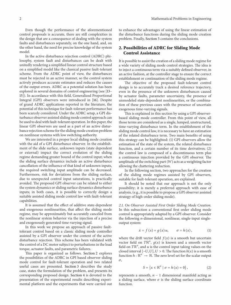
Figure 2 Time response of the control systems under the load-torque perturbations From top to bottom speed control response controlsignal and load-torque perturbation
where the estimates 120585 and 119889119889119905 are also provided by GPIobserver (43)
Finally the following discontinuous feedback control lawis considered
119906 =1
120581[minus120585120590minus119882 sign (120590)] (49)
4 Experimental Results
In this section we describe the experiments that were carriedout to assess the performance of the proposed GPI observerassisted sliding mode control (SMC+GPIobs) against theclassic sliding mode control (SMC) applied to a mechatronicsystem affected by perturbations and faults First the experi-mental setup is described then two different operation cases
are exposed and analyzed under a tracking problem systemwith perturbations and system with faults
41 Experimental Setup The designed controllers wereimplemented in a MATLAB xPC Target environment usinga sampling period of 01ms on a computer equipped with aPentium D processor The connection between the mecha-tronic system and each controller was performed by twoNational Instruments PCI-6024E data acquisition cards APWM output at 8000Hz and a digital output were both usedto command each DC-motor full-bridge driver one PWMinput was used to read the main-motor encoder frequencytwo digital outputs were used for enablingdisabling thefaults and an analog input was used to read the load-motorcurrent sensor output
Mathematical Problems in Engineering 9
0 20 40 60 8005
1
15
2Speed control with faults
Spee
d (r
evs
)
Time (s)
DC-bus faultChange in Ra
(a)
Time (s)0 20 40 60 80
05
1
15
2Speed control with faults
Spee
d (r
evs
) DC-bus faultChange in Ra
(b)
0 20 40 60 80
0
50Control signal
PWM
()
Time (s)
Setpoint
SMC W = 3000
SMC + GPIobsW = 50
minus50
(c)
PWM
()
0 20 40 60 80
0
50Control signal
Time (s)
Setpoint
SMC W = 5000
SMC + GPIobsW = 50
minus50
(d)
Figure 3 Time response of the control systems under faults 1 and 2 Fault 1 is applied at 119905 = 30 and fault 2 is applied at 119905 = 40
Fault 1 consists of increasing the armature resistance ofthe main-motor when this fault is enabled the armatureresistance of themotor is increased by 80 (119877af = 47 ohms)This fault is enabled (when applicable) at 119905 = 30 secFault 2 consists of changing the DC-level of the main-motorfull-bridge driver power supply When this fault goes fromdisabled to enabled theDC-level of the power supply changesfrom 30Vdc to 20VdcThis fault is enabled (when applicable)at 119905 = 40 sec
The parameters of the controller are defined as follows120581 = 1556 120582
0= 100 119882 = 50 119897
3= 320 119897
2= 26400 119897
1=
128000 and 1198970= 160000
42 Experimental Results under Perturbations Figure 2shows the experimental results of the control systemsunder evaluation using a setpoint defined as 120596lowast
119903(119905) =
03 sin(025120587119905) + 13 In this case the control systems areaffected by load torque disturbances The perturbationsapplied to the main-motor are showed in Figures 2(e) and2(f) Notice that the same perturbation profile is applied toall control schemes in evaluation
The plots of (a) (c) and (e) in the first column ofFigure 2 depict the experiments of the control systems using119882 = 3000 for SMC and 119882 = 50 for SMC+GPIobs Theplots (b) (d) and (f) of Figure 2 in the last column depictthe experiments using119882 = 5000 for SMC and119882 = 50 forSMC+GPIobs Figure 2(a) shows that the classic SMC (inblue) is highly affected by the perturbations Although theswitching gain was fixed in 119882 = 3000 the control system
gets out of the slidingmodemany times and the tracking per-formance is reduced Notice that the tracking performanceand disturbance rejection may be improved by increasing theswitching gain119882 however under this condition the chatter-ing phenomenon will be more problematic (see Figure 2(b))
On the other hand the proposed GPI observer assistedSMC was capable of rejecting the perturbations and thetracking performance was maintained In this case theswitching gain119882was reduced to119882 = 50 which was allowedby the use of the GPI observer that assists the sliding modecontroller Figures 2(c) and 2(d) show that the control signalfor SMC+GPIobs (in green) has less control effort than theclassic SMC scheme The chattering in the controlled speedwas attenuated even in the presence of unknown perturba-tions as seen in Figures 2(a) and 2(b) (in green)
43 Experimental Results under Faults Figure 3(a) showsthat in presence of fault 1 at 119905 = 30 the tracking per-formance of the classic SMC (in blue) is degraded Theselection of 119882 = 3000 in the classic SMC allows set-point tracking with no faults however it is not possibleto maintain the sliding mode for the tracking trajectorywhen the fault is enabled Meanwhile the GPI observerassisted SMC (in green) is capable of tolerating the first faultand even of keeping the tracking performance almost withno change Note that the switching gain of the proposedstrategy is very low (119882 = 50) which is beneficial forchattering reduction It is important to observe that at
10 Mathematical Problems in Engineering
0 20 40 60 8005
1
15
2Sp
eed
(rev
s)
Sliding mode control
Time (s)
W = 7000
0 20 40 60 8005
1
15
2
Spee
d (r
evs
)
Time (s)
W = 5500
0 20 40 60 8005
1
15
2
Spee
d (r
evs
)
Time (s)
W = 3500
0 20 40 60 8005
1
15
2
Spee
d (r
evs
)
Time (s)
W = 2500
0 20 40 60 8005
1
15
2
Time (s)
Spee
d (r
evs
)
W = 2000
(a)
0 20 40 60 8005
1
15
2
Spee
d (r
evs
)
GPI observer assisted sliding mode control
Time (s)
W = 2500
0 20 40 60 8005
1
15
2
Spee
d (r
evs
)
Time (s)
W = 1000
0 20 40 60 8005
1
15
2
Spee
d (r
evs
)
Time (s)
W = 250
0 20 40 60 8005
1
15
2
Spee
d (r
evs
)
Time (s)
W = 100
0 20 40 60 8005
1
15
2
Time (s)
Spee
d (r
evs
)
W = 10
(b)
Figure 4 Time response of the control systems (no faults and no perturbations) under variations in the switching gain119882 In the first columnsliding mode control in the second column GPI observer assisted sliding mode control
the time of the fault (119905 = 30) there is a tiny transientresponse in the controlled speed to recover the sliding regimeagain
Figure 3(a) also shows the effect of fault 2 in the controlledspeed at 119905 = 40 At this point it is noticed that after the faultis applied the classic SMC (in blue) is not capable of main-taining the sliding regime and its tracking performance ishighly degraded Moreover the GPI observer assisted SMC
(in green) tolerates the fault and quickly restores its trackingperformance without increasing the chattering
Figures 3(b) and 3(d) show the experimental results using119882 = 5000 for the classic SMC compared to the proposed GPIobserver assisted SMC In this case the classic SMC can toler-ate fault 1 at 119905 = 30 however a notable increasing in the chat-tering is observed On the other hand when fault 2 is appliedat 119905 = 40 the classic SMC cannot tolerate it
Mathematical Problems in Engineering 11
44 Chattering Reduction Figure 4 shows that both controlsystems in evaluation track the setpoint when no faultsand no perturbations are applied However the classic SMCrequires larger switching gains to track the given setpointThis issue notably increases the chattering phenomenon inthe main-motor controlled speed compared to the proposedGPI observer assisted SMC In the proposed assisted SMCscheme the chattering is alleviated by reducing the switchinggain down to 119882 = 10 without loss of the sliding modeFigure 4 shows that the use of the GPI observer to assistthe SMC allows reducing the switching gain 119882 thus thechattering problem is alleviated
5 Conclusions
In this paper an extension of Generalized Proportional Inte-gral observer-based control has been proposed to the prob-lem of robust creation of sliding regimes for nonlinear single-input single-output systems with limited switching controlinput authority for fault-tolerant operation The approachconsiders the use of a GPI observer for the accurate (linear)estimation of nonlinear endogenous as well as exogenousdisturbance inputs affecting the existence of local slidingregimes on a given smooth sliding manifold Active on-linedisturbance estimation and subsequent cancellation of state-dependent and time-dependent disturbances significantlycontribute to reducing the required switching control ampli-tude needed to sustain a sliding regime As an additionalbonus it experimented a chattering reduction
It was shown through the experimental tests that theproposedGPI observer assisted slidingmode control strategyis capable of maintaining the sliding regime even under hardoperating conditions such as system uncertainties perturba-tions actuator faults parametric failures and small switchingcontrol input authority This demonstrates the robustness ofthe proposed strategy accomplished by a simple linear GPIobserver-based control working on an ADRC paradigm
It was experimentally probed that (a) the proposed GPIobserver-based SMC strategy allows reducing the chatteringin the controlled variable (limited by the lumped perturba-tion estimation error) and (b) the proposed strategy forcesthe system to approximately keep its nominal performancein the presence of perturbations faults and uncertainties
Acknowledgments
The authors gratefully acknowledge the support for the real-ization of this work from the following institutions Univer-sidad Nacional de Colombia Cinvestav-IPN and UPIITA-IPN
References
[1] C Edwards H Alwi and C P Tan ldquoSliding mode methods forfault detection and fault tolerant controlrdquo in Proceedings of the1st Conference onControl and Fault-Tolerant Systems (SysTol rsquo10)pp 106ndash117 Nice France October 2010
[2] H Alwi and C Edwards ldquoFault detection and fault-tolerantcontrol of a civil aircraft using a sliding-mode-based schemerdquo
IEEE Transactions on Control Systems Technology vol 16 no 3pp 499ndash510 2008
[3] B Xiao Q Hu and Y Zhang ldquoAdaptive sliding mode faulttolerant attitude tracking control for flexible spacecraft underactuator saturationrdquo IEEE Transactions on Control SystemsTechnology vol 20 no 6 pp 1605ndash1612 2012
[4] M T Hamayun C Edwards and H Alwi ldquoIntegral slidingmode fault tolerant control incorporating on-line control allo-cationrdquo in Proceedings of the 11th International Workshop onVariable Structure Systems (VSS rsquo10) pp 100ndash105 Mexico CityMexico June 2010
[5] M Chen and W-H Chen ldquoSliding mode control for a classof uncertain nonlinear system based on disturbance observerrdquoInternational Journal of Adaptive Control and Signal Processingvol 24 no 1 pp 51ndash64 2010
[6] W Wang and Z-M Bai ldquoSliding mode control based ondisturbance observer for servo systemrdquo inProceedings of the 2ndInternational Conference on Computer and Automation Engi-neering (ICCAE rsquo10) vol 2 pp 26ndash29 Singapore February 2010
[7] D Tian D Yashiro and K Ohnishi ldquoImproving transparencyof bilateral control system by sliding mode assist disturbanceobserverrdquo IEEJ Transactions on Electrical and Electronic Engi-neering vol 8 no 3 pp 277ndash283 2013
[8] J Yang S Li and X Yu ldquoSliding-mode control for systems withmismatched uncertainties via a disturbance observerrdquo IEEETransactions on Industrial Electronics vol 60 no 1 pp 160ndash1692013
[9] M Shi X Liu Y Shi W Chen and Q Zhao ldquoResearch on thesliding mode based ADRC for hydraulic active suspension of asix-wheel off-road vehiclerdquo in Proceedings of the InternationalConference on Electronic and Mechanical Engineering andInformation Technology (EMEIT rsquo11) vol 2 pp 1066ndash1069Heilongjiang China August 2011
[10] V S Deshpande M Bhaskara and S B Phadke ldquoSlidingmode control of active suspension systems using a disturbanceobserverrdquo in Proceedings of the 12th International Workshop onVariable Structure Systems (VSS rsquo12) pp 70ndash75 2012
[11] Y Cao and X B Chen ldquoDisturbance-observer-based sliding-mode control for a 3-dof nanopositioning stagerdquo in Proceedingsof the IEEEASME Transactions onMechatronics vol PP no 99pp 1ndash8 Mumbai India 2013
[12] D-J Zhao Y-J Wang L Liu and Z-S Wang ldquoRobust fault-tolerant control of launch vehicle via GPI observer and integralslidingmode controlrdquoAsian Journal of Control vol 15 no 2 pp614ndash623 2013
[13] Z Gao Y Huang and J Han ldquoAn alternative paradigm forcontrol system designrdquo in Proceedings of the 40th IEEE Confer-ence on Decision and Control (CDC rsquo01) vol 5 pp 4578ndash4585December 2001
[14] G Tian and Z Gao ldquoFrom ponceletrsquos invariance principle toactive disturbance rejectionrdquo in Proceedings of the AmericanControl Conference (ACC rsquo09) pp 2451ndash2457 June 2009
[15] J Han ldquoFromPID to active disturbance rejection controlrdquo IEEETransactions on Industrial Electronics vol 56 no 3 pp 900ndash906 2009
[16] H Sira-Ramırez and V F Batlle ldquoRobust Σ minus Δ modulation-based sliding mode observers for linear systems subject to timepolynomial inputsrdquo International Journal of Systems Science vol42 no 4 pp 621ndash631 2011
[17] V Utkin J Guldner and J Shi Sliding Mode Control in Electro-Mechanical Systems CRC Press Boca Raton Fla USA 2ndedition 2009
12 Mathematical Problems in Engineering
[18] H Sira-Ramırez and S K Agrawal Differentially Flat SystemsMarcel Dekker 2004
[19] Y Gliklikh ldquoNecessary and suffcient conditions for global-in-time existence of solutions of ordinary stochastic and parabolicdifferential equationsrdquo Abstract and Applied Analysis vol 2006Article ID 39786 17 pages 2006
[20] H Sira-Ramırez A Luviano-Juarez and J Cortes-RomeroldquoControl lineal robusto de sistemas no lineales diferencial-mente planosrdquo RIAI Revista Iberoamericana de Automatica eInformatica Industrial vol 8 no 1 pp 14ndash28 2011
[21] H Coral-Enriquez J Cortes-Romero and A G RamosldquoRobust active disturbance rejection control approach to max-imize energy capture in variable-speed wind turbinesrdquo Mathe-matical Problems in Engineering vol 2013 Article ID 396740 12pages 2013
[22] R Isermann Fault-Diagnosis Applications Springer BerlinGermany 2011
[23] J H Lee and J Lyou ldquoFault diagnosis and fault tolerant con-trol of dc motor driving systemrdquo in Proceedings of the IEEEInternational Symposium on Industrial Electronics (ISIE rsquo01) vol3 pp 1719ndash1723 2001
[24] G Grandi P Sanjeevikumar Y Gritli and F Filippetti ldquoFault-tolerant control strategies for quad inverter induction motordrives with one failed inverterrdquo in Proceedings of the 20thInternational Conference on Electrical Machines (ICEM rsquo12) pp959ndash966 2012
[25] C C deWit H Olsson K J Astrom and P Lischinsky ldquoA newmodel for control of systems with frictionrdquo IEEE Transactionson Automatic Control vol 40 no 3 pp 419ndash425 1995
Submit your manuscripts athttpwwwhindawicom
Hindawi Publishing Corporationhttpwwwhindawicom Volume 2014
MathematicsJournal of
Hindawi Publishing Corporationhttpwwwhindawicom Volume 2014
Mathematical Problems in Engineering
Hindawi Publishing Corporationhttpwwwhindawicom
Differential EquationsInternational Journal of
Volume 2014
Applied MathematicsJournal of
Hindawi Publishing Corporationhttpwwwhindawicom Volume 2014
Probability and StatisticsHindawi Publishing Corporationhttpwwwhindawicom Volume 2014
Journal of
Hindawi Publishing Corporationhttpwwwhindawicom Volume 2014
Mathematical PhysicsAdvances in
Complex AnalysisJournal of
Hindawi Publishing Corporationhttpwwwhindawicom Volume 2014
OptimizationJournal of
Hindawi Publishing Corporationhttpwwwhindawicom Volume 2014
CombinatoricsHindawi Publishing Corporationhttpwwwhindawicom Volume 2014
International Journal of
Hindawi Publishing Corporationhttpwwwhindawicom Volume 2014
Operations ResearchAdvances in
Journal of
Hindawi Publishing Corporationhttpwwwhindawicom Volume 2014
Function Spaces
Abstract and Applied AnalysisHindawi Publishing Corporationhttpwwwhindawicom Volume 2014
International Journal of Mathematics and Mathematical Sciences
Hindawi Publishing Corporationhttpwwwhindawicom Volume 2014
The Scientific World JournalHindawi Publishing Corporation httpwwwhindawicom Volume 2014
Hindawi Publishing Corporationhttpwwwhindawicom Volume 2014
Algebra
Discrete Dynamics in Nature and Society
Hindawi Publishing Corporationhttpwwwhindawicom Volume 2014
Hindawi Publishing Corporationhttpwwwhindawicom Volume 2014
Decision SciencesAdvances in
Discrete MathematicsJournal of
Hindawi Publishing Corporationhttpwwwhindawicom
Volume 2014
Hindawi Publishing Corporationhttpwwwhindawicom Volume 2014
Stochastic AnalysisInternational Journal of
2 Mathematical Problems in Engineering
Even though the performance of the aforementionedcontrol proposals is accurate there are still complexities inthe design that are a consequence of dealing with the systemfaults and disturbances separately on the one hand and onthe other hand the need for precise knowledge of the systemmodel
In the active disturbance rejection control (ADRC) phi-losophy system fault and disturbances can be dealt withunitedly rendering a simplified linear control structure basedon a simplified model like the classical passive fault-tolerantscheme From the ADRC point of view the disturbancesmust be rejected in an active manner so the control systemactively produces accurate estimates and reduces the causesof the output errors ADRC as a potential solution has beenexplored in several domains of control engineering (see [13ndash15]) In accordance with this field Generalized ProportionalIntegral (GPI) observers were introduced in [16] Despiteof grand ADRC applications reported in the literature thepotential of this technique for fault-tolerant performance hasbeen scarcely considered Under the ADRC setup a GPI dis-turbance observer assisted slidingmode control approach canbe used to deal with fault-tolerant operation In this paper thelinear GPI observers are used as a part of an active distur-bance rejection scheme for the slidingmode creation problemon nonlinear systems with low switching authority
We are interested in a proper local sliding mode creationwith the aid of a GPI disturbance observer In the establish-ment of the slide surface unknown inputs (state dependentor external) impact the correct evolution of the slidingregime demanding greater bound of the control input whenthe sliding surface dynamics include an active disturbancecancellation of the influence of that kind of unknown inputsthe required switching input amplitude can be decreasedFurthermore risk for deviations from the sliding surfacedue to unexpected control input saturations is practicallyavoided The proposed GPI observer can be related to eitherthe system dynamics or sliding surface dynamics disturbanceinputs in both cases it is possible to correctly design asuitable assisted sliding mode control law with fault-tolerantcapabilities
It is assumed that the effect of additive state-dependentand exogenous nonlinearities that affect the sliding moderegime may be approximately but accurately canceled fromthe nonlinear system behavior via the injection of a preciseand exogenously generated time-varying signal
In this work we propose an approach of passive fault-tolerant control based on a classic sliding mode controllerassisted by a GPI observer under the context of the activedisturbance rejection This scheme has been validated withthe control of a DCmotor subject to perturbations in the loadtorque actuator faults and parametric failures
This paper is organized as follows Section 2 exploresthe possibilities of the ADRC in GPI based observer slidingmode control for fault-tolerant operation and two relateduseful cases are presented Section 3 describes the studycase states the formulation of the problem and presents itscorresponding proposed design Section 4 is devoted to thepresentation of the experimental results describing experi-mental platform and the experiments that were carried out
to enhance the advantages of using the linear estimation ofthe disturbance functions during the sliding mode creationproblem Finally Section 5 contains the conclusions
2 Possibilities of ADRC for Sliding ModeControl Assistance
It is possible to assist the creation of a slidingmode regime fora wide variety of sliding mode control strategies The idea isto inject a continuous term via a suitably defined observer inan active fashion at the controller stage to ensure the correctestablishment or continuation of the sliding mode regime
The objective of the proposed fault-tolerant controldesign is to accurately track a desired reference trajectoryeven in the presence of the unknown disturbances causedby actuator faults parameter uncertainty the presence ofunmodeled state-dependent nonlinearities or the combina-tion of these previous cases with the presence of uncertainexogenous time-varying signals
This is explained in this section by using a GPI observer-based sliding mode controller From this point of view allthose terms are considered as a single lumped unstructuredtime-varying disturbance term In the establishment of theslidingmode control law it is necessary to have an estimationof the related disturbance term Two main benefits of usingthis strategy can be highlighted (1) GPI observers allow theestimation of the state of the system the related disturbancefunction and a certain number of its time derivatives (2)the control law is composed of a discontinuous term plusa continuous injection provided by the GPI observer Theamplitude of the switching part (119882) acts as a weighting factorallowing the chattering reduction
In the following section two approaches for the creationof the sliding mode regimes assisted by GPI observerssuitable for fault-tolerant operation are explained
It should be noted that our approach is not the onlypossibility it is merely a preferred approach with ease ofanalysis (eg it is possible to propose a GPI observer assistedstrategy of high-order sliding mode)
21 On Observer Assisted First Order Sliding Mode CreationIn this subsection a conventional first order sliding modecontrol is appropriately adapted by a GPI observer Considerthe following 119899-dimensional nonlinear single-input single-output system
= 119891 (119909) + 119892 (119909) 119906 120590 = ℎ (119909) (1)
where the drift vector field 119891(119909) is a smooth but uncertainvector field on 119879R119899 119892(119909) is known and a smooth vectorfield on 119879R119899 and 119906 is the control input taking values on theclosed interval [minus119880119880]119880 gt 0 The function ℎ(119909) is a smoothfunction ℎ R119899 rarr R The zero level set for the scalar output120590
119878 = 119909 isin R119899
| 120590 = ℎ (119909) = 0 (2)
represents a smooth 119899 minus 1 dimensional manifold acting asa sliding surface where 120590 is the sliding surface coordinatefunction
Mathematical Problems in Engineering 3
The state-dependent unperturbed sliding surface dynam-ics are characterized by
= 119871119891ℎ (119909) + 119871
119892ℎ (119909) 119906 (3)
where 119871119891and 119871
119892are the Lie derivatives or the directional
derivatives of ℎ along the directions of the vectors 119891 and 119892respectively
Actuator faults exogenous disturbances modeled andnon modeled internal dynamics and possible parametervariation can be treated as an equivalent additive lumped dis-turbance function 120585
120590 affecting the sliding surface dynamic120590
= 120585120590+ 119871119892ℎ (119909) 119906 (4)
211 Assumptions
Assumption 1 The amplitude119882 of the switching part of thecontrol input 119906 satisfies119882 lt 119880
Assumption 2 The disturbance function 120585120590 and a finite
number of its time derivatives 120585(119896)120590 119896 = 0 1 2 119898 for a
sufficiently large 119898 are assumed to be uniformly and abso-lutely bounded that is 0 le |120585(119896)
120590| le 120575119896lt infin for any feedback
control input stabilizing the sliding surface coordinatedynamics
Assumption 3 Weassume that119871119892ℎ(119909) gt 0 is perfectly known
and locally strictly positiveThe key observation for the robust operation of the
proposed sliding regimes is based on the accurate yetapproximate on-line estimation of the scalar uncertain dis-turbance function 120585
120590in the form 120585
120590 The incorporation of
that estimation in the slidingmode control lawmay result in asubstantially enhanced possibility for the creation of a slidingmotion via the active disturbance cancelation strategy
119906 =1
119871119892ℎ (119909)
[minus120585120590minus119882 sign (120590)] (5)
An extended state representation can be proposed tocope with the disturbance function estimation 120585
120590 The aug-
mented representation is based on the internal model ofthe disturbance function 120585
120590 When there is no previous
knowledge about the disturbance term 120585120590 a general signal
oriented approach can be quite effective for on-line estima-tion purposes Associated with ADRC and specialized byGPIapproaches unknown input signals can be approximated by119889119898
120585120590119889119905119898
asymp 0 For that realization the extended state vector119909120590= [120590 120585
120590120585(1)
120590sdot sdot sdot 120585(119898minus1)
120590]119879
is considered Therefore theextended state space representation is given by
120590= 1198601119909120590+ 119861120590119871119892ℎ (119909) 119906 + 119864
120590120585(119898)
(6)
where
1198601=
[[[[[[
[
0 1 0 sdot sdot sdot 0
0 0 1 0
d
0 0 0 sdot sdot sdot 1
0 0 0 sdot sdot sdot 0
]]]]]]
]
119861120590=
[[[[[[
[
1
0
0
0
]]]]]]
]
119864120590=
[[[[[[
[
0
0
0
1
]]]]]]
]
(7)
The disturbance function estimation is given by thefollowing GPI observer
Theorem 1 Letting 119911 = [11991111199112sdot sdot sdot 119911119898+1]119879 and Γ =
[120574119898120574119898minus1
sdot sdot sdot 1205740]119879 with Assumptions 1ndash3 the following
observer for system (4) = 119860
1119911 + 119861120590119871119892ℎ (119909) 119906 + Γ119890
120590(8)
with119898 being a sufficiently large integer produces exponentiallyasymptotic estimation of 120590 120585
120590 120585
(119898minus1)
120590given by the observer
variables 1199111 1199112 119911
119898 respectively The estimation errors (120590minus
1199111) (120585120590minus 1199112) (120585
(119898minus1)
120590minus 119911119898+1) are ultimately uniformly
bounded given the design parameters 1205740 120574
119898that are chosen
so that the following characteristic polynomial is Hurwitz
119901119890120590
(119904) = 119904119898+1
+ 120574119898119904119898
+ sdot sdot sdot + 1205741119904 + 1205740 (9)
Proof The corresponding estimation error vector is definedas 119890120590= 119909120590minus 119911 and satisfies
119890120590= (1198601minus 119871119862) 119890
120590+ 119864120590120585(119898)
= 119860120590119890120590+ 119864120590120585(119898)
(10)
with
119860120590=
[[[[[[
[
minus120574119898
1 0 sdot sdot sdot 0
minus120574119898minus1
0 1 0
dminus1205741
0 0 sdot sdot sdot 1
minus1205740
0 0 sdot sdot sdot 0
]]]]]]
]
isin R(1+119898)times(1+119898)
(11)
and its characteristic polynomial in the complex variable 119904 isgiven by
119901119890120590
(119904) = det (119904119868 minus 119860120590) = 119904119898+1
+ 120574119898119904119898
+ sdot sdot sdot + 1205741119904 + 1205740 (12)
where the eigenvalues of 119860120590can be placed as desired by
selecting the gain vector Γ The Hurwitzian character of 119860120590
implies that for every constant (1+119898)times (119899+119898) symmetricpositive definitematrix119876 = 119876119879 gt 0 there exists a symmetricpositive definite (1 +119898) times (1 +119898)matrix 119875 = 119875119879 gt 0 so that119860119879
120590119875 + 119875119860
120590= minus119876 The Lyapunov function candidate 119881(119909) =
(12)119890119879
120590119875119890120590exhibits a time derivative alongwith the solutions
of the closed loop system given by
(119890120590 119905) =
1
2119890119879
120590(119860119879
120590119875 + 119875119860
120590) 119890120590+ 119890119879
120590119875119864120590120585(119898)
120590(119905) (13)
For 119876 = 119868 that is an (1 + 119898) times (1 + 119898) identity matrix thisfunction satisfies
(119909120590 119905) =
1
2119890119879
120590(minus119876) 119890
120590+ 119890119879
120590119875119864120590120585(119898)
120590(119905)
le1
2
10038171003817100381710038171198901205901003817100381710038171003817
2
2+10038171003817100381710038171198901205901003817100381710038171003817211987521198642120575119898
(14)
4 Mathematical Problems in Engineering
Given that 1198642= 1 and according to Assumption 2 this
function is strictly negative everywhere outside the sphere 119878120590
given by
119878120590= 119890120590isin 1198771+119898
|100381710038171003817100381711989012059010038171003817100381710038172le 21205751198981198752 (15)
Hence all trajectories 119890120590(119905) starting outside this sphere
converge towards its interior and all those trajectories start-ing inside 119878
120590will never abandon it
Corollary 2 Under all the previous assumptions the discon-tinuous active disturbance rejection feedback controller
119906 =1
119871119892ℎ (119909)
[minus1199111minus119882 sign (120590)] (16)
locally creates a sliding regime for any amplitude119882 satisfying119882 gt 120575
0 with 120575
0as the ultimate bound for the disturbance
estimation error 119890120590
Proof The observer-based control law renders the followingclosed loop sliding surface dynamics
= (120585120590minus 120585120590) minus119882 sign (120590) (17)
with 120585120590= 1199111 which would require a smaller control input
switching amplitude119882 than in the case where the observer isnot used According toTheorem 1 the disturbance estimationerror 119890
120590 is bounded by 120575
1 and the local existence of a sliding
regime 120590 = 0 is guaranteed even if119882 is rather smallConsider the following Lyapunov function candidate
119881 =1
21205902
(18)
Differentiating the Lyapunov function (18) with respect totime and using (17) yield
= 120590
= 120590 (120585120590minus 120585120590minus119882 sign (120590))
= 120590 (120585120590minus 120585120590) minus119882 |120590|
le |120590| 1205750minus119882 |120590|
(19)
is strictly negative if119882 gt 1205750 Therefore if119882 gt 120575
0 locally
it creates a sliding regime (see [17])
22 Observer Assisted Nonlinear Controlled Systems in Input-Output Representation In the previous subsection the powerof the GPI observer injections for a proper establishmentand development of a first order sliding mode regimen wasdemonstrated In this subsection the GPI observer is used ina wider perspective allowing both sliding surface coordinatefunction (120590) and disturbance function (120585
120590) constructions
These constructions are conducted by means of the systemstate estimation and disturbance function estimation relatedto system dynamics all are supplied by the GPI observer
Consider the nonlinear scalar differentially flat system
119910(119899)
= 120595 (119905 119910) 119906 + 120601 (119905 119910 119910 119910(119899minus1)
) (20)
with the following set of initial conditions 1198840= 119910(119905
0)
119910(1199050) 119910
(119899minus1)
(1199050) We refer to the function 120595(119905 119910) as the
control input gain of the system The term 120601(119905 119910 119910
119910(119899minus1)
) will be addressed as the drift functionFor a given smooth control input function 119906(119905) let 119910(119905) =
Θ(119905 1199050 1198840 119906(119905)) denote the solution trajectory of system (20)
from the set of initial conditions 1198840 We denote by the time
function 120585(119905) the additive disturbance function regardless ofany particular internal structure
It is desired to drive the flat output 119910 of the system
119910(119899)
= 120595 (119905 119910) 119906 + 120585 (119905) (21)
to track a given smooth reference trajectory 119910lowast(119905) regardlessof the unknown but uniformly bounded nature of thedisturbance function 120585(119905) As in the previous case 120585 takesinto account in a lumped way faults and exogenous andendogenous disturbances affecting the system dynamics Itis important to note that the disturbance functions 120585 and 120585
120590
are defined in different dynamics but catch the same essentialdisturbance behavior Indeed it will be showed that it ispossible to form an estimate of 120585
120590from an estimate of 120585 and
some others estimates provided by the GPI observerRegarding controlled system (21) we make the following
assumptions
Assumption 4 The disturbance function 120585(119905) is completelyunknown while the control input gain 120595(119905 119910) is perfectlyknown Let 120598 be a strictly positive real number The controlinput gain 120595(119905 119910) is assumed to be uniformly bounded awayfrom zero that is inf
119905|120595(119905 119910)| ge 120598 gt 0 for any solution 119910(119905) of
the controlled system In particular it is bounded away fromzero for the given output reference trajectory 119910lowast(119905)
Assumption 5 It is assumed that a solution 119910(119905) existsuniformly in 119905 for every given set of initial conditions 119884
0
specified at time 119905 = 1199050and for a given sufficiently smooth
control input function 119906(119905) Given a desired flat outputreference trajectory 119910lowast(119905) the flatness of the system and theprevious assumption a straightforward calculation of the cor-responding (unique) open loop control input 119906lowast(119905) is possible(see [18])
Assumption 6 Let 119898 be a given integer As a time functionthe 119898th time derivative of 120585(119905) is uniformly absolutelybounded In other words there exists a constant119870
119898so that
sup119905
10038161003816100381610038161003816120585(119898)
(119905)10038161003816100381610038161003816le 119870119898 (22)
Remark 3 Assumption 6 cannot be verified a priori when120585(119905) is completely unknown However in cases where thenonlinearity is known except for some of its parameters itsvalidity can be assessed with some work Also if 120585(119898)(119905) isnot uniformly absolutely bounded almost everywhere thensolutions 119910(119905) for (21) do not exist for any finite 119906(119905) (see [19])
Mathematical Problems in Engineering 5
221 Observer-Based Approach With reference to simplifiedsystem (21) in order to propose a GPI observer for a relatedstate and disturbance function estimation it is consideredthat the internal model of the disturbance function 120585 isapproximated by 119889119898120585(119905)119889119905119898 asymp 0 at the observer stageThismodel is embedded into the augmentedmodel which is char-acterized by an extended state composed of the phase vari-ables119909
1 1199092 119909
119899 associatedwith the flat output119909
1= 119910 and
augmented by the119898 output estimation error iterated integralinjections 119909
119899+1 119909
119899+119898 As a result setting the state vector
119909 = [11990911199092sdot sdot sdot 119909
119899+119898] with 119909
1= 119910 119909
2= 119910 119909
119899= 119910(119899minus1)
119909119899+1
= 120585 119909119899+119898
= 120585(119898minus1) the augmented state spacemodel
is given by
= 119860119909 + 119861120595 (119905 119910) 119906 + 119864120585(119898)
119910 = 119862119909
(23)
with
119860 =
[[[[[[
[
0 1 0 sdot sdot sdot 0
0 0 1 0
d0 0 0 sdot sdot sdot 1
0 0 0 sdot sdot sdot 0
]]]]]]
]
isin R(119899+119898)times(119899+119898)
119861 =
[[[[[[[
[
0
1(119899th position)
0
]]]]]]]
]
isin R(119899+119898)times1
119862 = [1 0 sdot sdot sdot 0] isin R1times(119899+119898)
119864 =
[[[[[[
[
0
0
0
1
]]]]]]
]
isin R(119899+119898)times1
(24)
Now the GPI observer for the state 119909 is proposed
119909 = 119860119909 + 119861120595 (119905 119910) 119906 + 119871 (119910 minus 119910)
119910 = 119862119909
(25)
where 119909 = [11990911199092
sdot sdot sdot 119909119899+119898]119879 is the estimation
state vector and the observer gain vector is 119871 =
[119897119899+119898minus1
sdot sdot sdot 11989711198970]119879
The estimation error vector 119890119909= [11989011990911198901199092sdot sdot sdot 119890119909(119899+119898)
]119879
defined as 119890119909= 119909 minus 119909 satisfies
119890119909= (119860 minus 119871119862) 119890
119909+ 119864120585(119898)
119890119909= 119860119890119890119909+ 119864120585(119898)
(26)
where
119860119890=
[[[[[[
[
minus119897119899+119898minus1
1 0 sdot sdot sdot 0
minus119897119899+119898minus2
0 1 0
dminus1198971
0 0 sdot sdot sdot 1
minus1198970
0 0 sdot sdot sdot 0
]]]]]]
]
(27)
with 119860119890isin R(119899+119898)times(119899+119898) and its characteristic polynomial in
the complex variable 119904 is given by
119901119890119909
(119904) = det (119904119868 minus 119860119890)
= 119904119899+119898
+ 119897119899+119898minus1
119904119899+119898minus1
+ sdot sdot sdot + 1198971119904 + 1198970
(28)
Theorem 4 Suppose that all previous assumptions are validLet the coefficients 119897
119895 with 119895 = 0 1 119899 + 119898 minus 1 of the
polynomial 119901119890119909
(119904) be chosen so that all their roots are exhibitedto the left of the complex plane C Then the trajectories of theestimation error vector 119890
119909(119905) globally converge towards a small
as-desired sphere of radius 120588 denoted by 119878(0 120588) centered at theorigin of the estimation error phase space 119890
1199091 1198901199092 119890
119909(119899+119898)
where they remain ultimately bounded
Proof This problem has already been proposed with slightlydifferent notation in [20] In a recent work [21] it is shownthat the estimation error vector is uniformly ultimatelybounded
Remark 5 Consequently with Theorem 4 the variables119909119899+1 119909119899+2 119909
119899+119898track arbitrarily and closely the unknown
time functions 120585(119905) and their time derivatives 120585(119895)(119905) 119895 =
1 119898 minus 1
222 Sliding Surface Design Regarding controlled systems(21) a conventional sliding surface can be chosen as (in orderto decrease the stable error an integral term of the trackingerror 119890
119910can be introduced (see [12]) but it is preferred to
maintain a conventional surface to enhance the GPI observercapabilities)
120590 = 119890(119899minus1)
119910+ 120582119899minus2119890(119899minus2)
119910+ sdot sdot sdot + 120582
0119890119910
(29)
with 119890119910= 119910 minus 119910
lowast being flat output tracking error The designparameters 120582
0 120582
119899minus2are chosen so that the characteristic
polynomial 119901120590(119904) = 119904
(119899minus1)
+ 120582119899minus2119904(119899minus2)
+ sdot sdot sdot + 1205820is Hurwitz
An estimated version of the previous surface can be givenby
= 119909119899minus [119910lowast
](119899minus1)
+ 120582119899minus2(119909119899minus1minus [119910lowast
](119899minus2)
)
+ sdot sdot sdot + 1205820(1199091minus 119910lowast
)
(30)
where 119910 = 1199091
119910(119899minus1) = 119909
119899are estimates provided by
GPI observer (8) The use of 1199091instead of 119909
1is preferred for
chattering reduction purposes (see [17])The sliding surface dynamics of is given by
120590 = 119909119899minus [119910lowast
](119899)
+ 120582119899minus2( 119909119899minus1minus [119910lowast
](119899minus1)
)
+ sdot sdot sdot + 1205820( 1199091minus 119910lowast
)
(31)
6 Mathematical Problems in Engineering
120579 120596
Host PC
Target PC with DAQ boards
MATLABSimulink
Perturbationgenerator Current
control
Fault profilegenerator
control
Signalconditioning
Periodmeasurement
PWMDirection
Analog input
DODO
PWMDirection
(A) signal
DC power supply30Vdc
Full-bridgedriver
Load-motor
Optocouplerrelay circuit
Load-motorshaft shaft
Coupling
Currentsensor
DC-bus level shift fault
DC power supply30Vdc 20Vdc
Faultoff
Faulton
Faultoff
Faulton
Full-bridgedriver
Main-
Main-motor
motor
Coupling
Rotaryencoder
(A B)
Parametric fault
Raf
ilowast(t)
i(t)
lowast(t)
lowast(t)
120596lowast(t)
120596(t)
Speed
Digital outputDigital output
+ +minus minus
Figure 1 General scheme of the experimental setup
On the other hand from the GPI Observer we have
119909119899= 120595 (119905 119910) 119906 + 119909
119899+1+ 119897119898(1199091minus 1199091) (32)
therefore
120590 = 120595 (119905 119910) 119906 + 120585120590
(33)
with
120585120590= 119909119899+1+ 119897119898(1199091minus 1199091) minus [119910
lowast
](119899)
+ 120582119899minus2( 119909119899minus1minus [119910lowast
](119899minus1)
) + sdot sdot sdot + 1205820( 1199091minus [119910lowast
](1)
)
(34)
where the estimates 119909119899minus1 119909
1are also provided by the GPI
observer Remember that as stated by the GPI observer statenotation 119909
119899+1= 120585 as announced at the beginning of this
subsection the disturbance function estimation related tosliding regime (33) 120585
120590is given in terms of 120585 which is related
to system dynamics (21)According to (5) the control law is
119906 =1
120595 (119905 119910)[minus120585120590minus119882 sign ()] (35)
Now consider the following Lyapunov function candi-date
1198811=1
22
(36)
Differentiating the Lyapunov function (36) with respectto time and using (33) and (35) we obtained
1= 120590 = (120595 (119905 119910) 119906 + 120585
120590) = minus119882 || (37)
which assures the sliding mode regime provided that119882 gt 0
3 Case Study
The system used for the experimental comparison of the pro-posed control strategies is a mechatronic system composedof two directly coupled DC motors The first motor (alsocalled the main-motor) acts as the system to be controlledThe second motor (also called the load-motor) generatesperturbation loads to the main-motor Hence the proposedcontrol strategies are applied to control the angular speed ofthemain-motor while the load-motor acts as the load-torqueperturbation generator by means of a current control loopFigure 1 shows a detailed scheme of the mechatronic systemcontrol loops and the experimental setup This figure alsoshows the implementation scheme of two faults armatureresistance fault (fault 1) and DC-bus level shift fault (fault 2)These faults are typical in systems as the one under study (asit will be explained later) and all controllers will be assessedunder these faults
31 Fault-Tolerant Control for DCMotors Themost commonfaults in DC-motor drives can be classified as actuatorparametric and sensor faults [22] The actuator faults aremainly due to the reduction in the performance of amplifiers
Mathematical Problems in Engineering 7
malfunction of power semiconductors and failures in regu-latory stages in the power supply [23 24] Parametric faultsare caused by degradation of brushes inertia and frictionchanges and variations in resistance or inductance of thearmature [22] This paper will consider two faults in themechatronic system
(1) parametric fault due to a change in the resistance ofDC-motor armature and
(2) actuator fault due to level shift of the DC-bus voltagethat feeds the full-bridge drive of the main-motor
32 Problem Formulation Consider the following dynamicmodel describing aDC-motor controlled by armature voltage119906(119905) with state variables given by 120596(119905) describing the rotorangular speed and 119894(119905) representing the armature current
119871119886
119889119894 (119905)
119889119905= 119896pwm119906 (119905) minus 119877119886119894 (119905) minus 119870119887120596 (119905)
119869119898
119889120596 (119905)
119889119905= 119870119879119894 (119905) minus 120591
119871(119905) minus 119861120596 (119905) minus 120575 (120596 (119905))
(38)
The parameters 119871119886and 119877
119886represent the armature induc-
tance and armature resistance 119869119898is the moment of inertia
119870119887is the back-emf constant 119870
119879is the torque constant 119861 is
the viscous friction coefficient 119896pwm is the conversion gain ofPWM 120591
119871represents the unknown load-torque perturbation
input 119906(119905) is the control signal and 120575(120596(119905)) represents anonlinear model of dry friction where119879
119888119879119904 and 120572 are terms
associated with coulomb friction (see [25]) Consider
120575 (120596) = 120596 [gt 119879119888sign (120596) + (119879
119904minus 119879119888) 119890minus120572|120596| sign (120596)]
(39)
By rewriting and lumping together some terms of (38)the following representation of the system (typical of theADRC paradigm) is obtained
(119905) = 120581119906 (119905) + 120585 (119905) (40)
where
120581 =
119870119879119896pwm
119869119898119871119886
120585 (119905) =119870119879
119869119898119871119886
[minus119877119886119894 (119905) minus 119870
119887120596 (119905)]
minus1
119869119898
119889120591119871
119889119905minus119861
119869119898
119889120596 (119905)
119889119905minus1
119869119898
119889120575 (120596 (119905))
119889119905
(41)
The problem is as follows Consider a DC-motordescribed by the dynamics presented in (40) where the rotorangular speed 120596(119905) is available for measurement Given asmooth reference trajectory 120596lowast(119905) for the angular velocityof the motor shaft find a control law 119906(119905) such that 120596(119905)is forced to track the given reference trajectory 120596lowast(119905) Thisobjective must be achieved even in the presence of unknowndisturbances represented by the load input torque 120591
119871 and the
effect of parametric and actuator faults
33 Disturbance GPI Observer Design The following approx-imation concerning the internal model of the distur-bance function 119889
2
120585(119905)1198891199052
asymp 0 is considered According tothis approximation the extended state vector is given by[120596 120585 120585]
119879 thus we obtain the following augmented plantmodel
[[[
[
120585
120585
]]]
]
=[[[
[
0 1 0 0
0 0 1 0
0 0 0 1
0 0 0 0
]]]
]
[[[
[
120596
120585
120585
]]]
]
+ 120581[[[
[
0
1
0
0
]]]
]
119906 +[[[
[
0
0
0
1
]]]
]
120585(2)
(42)
It is defined as an estimation error 119890120596= 120596 minus In order
to observe the augmented state a GPI observer is proposed
[[[[[[[[[[[[
[
119889
119889119905
119889120596
119889119905
119889120585
119889119905
119889120585
119889119905
]]]]]]]]]]]]
]
=[[[
[
0 1 0 0
0 0 1 0
0 0 0 1
0 0 0 0
]]]
]
[[[[
[
120596
120585
120585
]]]]
]
+ 120581[[[
[
0
1
0
0
]]]
]
119906 +[[[
[
1198973
1198972
1198971
1198970
]]]
]
119890120596 (43)
where [1198973119897211989711198970]119879 is the observer gains vector The char-
acteristic polynomial which describes the estimation errordynamics is defined as
119901119890119909
(119904) = 1199044
+ 11989731199043
+ 11989721199042
+ 1198971119904 + 1198970 (44)
Given the previously described uncertain model (42)linear GPI observer (43) estimates the augmented state[120596 120585 120585]
119879 with an arbitrary small phase space estimationerror provided that the set of observer design coefficients1198973 1198972 1198971 1198970 is chosen in such a manner that the roots of the
characteristic polynomial 119901119890120596
(119904) on the complex variable 119904are located sufficiently far from the imaginary axis in the lefthalf side of the complex plane
34 Sliding Control Law Design By defining the trackingerror as 119890
120596(119905) = 120596(119905) minus 120596
lowast
(119905) the following sliding surfacein terms of the tracking error 119890
120596are proposed
120590 = 119890120596+ 120582119890120596 (45)
A modified version of the sliding surface that usesestimates of 120596 and is proposed
= 120596 minus [120596lowast
](1)
+ 1205820( minus 120596
lowast
) (46)
where 120596(119905) and (119905) are estimations provided by a GPIobserver (43)
Applying time derivative to (46) the following dynamicsis obtained
120590 = 120581119906 + 120585120590
(47)
with
120585120590= 120585 + 119897
2(120596 minus ) minus [120596
lowast
](2)
+ 1205820(119889
119889119905minus [120596lowast
](1)
) (48)
8 Mathematical Problems in Engineering
0 20 40 60 8005
1
15
2Speed control with perturbations
Spee
d (r
evs
)
Time (s)
(a)
0 20 40 60 8005
1
15
2Speed control with perturbations
Spee
d (r
evs
)
Time (s)
(b)
0 20 40 60 80
0
50Control signal
PWM
()
Time (s)
minus50
(c)
0 20 40 60 80
0
50Control signal
PWM
()
Time (s)
minus50
(d)
Setpoint
0 20 40 60 80
0
05
1Perturbation load torque
Curr
ent (
A)
Time (s)
minus05
minus1
SMC W = 3000
SMC + GPIobsW = 50
(e)
0 20 40 60 80
0
05
1Perturbation load torque
Curr
ent (
A)
Time (s)
minus05
minus1
Setpoint
SMC W = 5000
SMC + GPIobsW = 50
(f)
Figure 2 Time response of the control systems under the load-torque perturbations From top to bottom speed control response controlsignal and load-torque perturbation
where the estimates 120585 and 119889119889119905 are also provided by GPIobserver (43)
Finally the following discontinuous feedback control lawis considered
119906 =1
120581[minus120585120590minus119882 sign (120590)] (49)
4 Experimental Results
In this section we describe the experiments that were carriedout to assess the performance of the proposed GPI observerassisted sliding mode control (SMC+GPIobs) against theclassic sliding mode control (SMC) applied to a mechatronicsystem affected by perturbations and faults First the experi-mental setup is described then two different operation cases
are exposed and analyzed under a tracking problem systemwith perturbations and system with faults
41 Experimental Setup The designed controllers wereimplemented in a MATLAB xPC Target environment usinga sampling period of 01ms on a computer equipped with aPentium D processor The connection between the mecha-tronic system and each controller was performed by twoNational Instruments PCI-6024E data acquisition cards APWM output at 8000Hz and a digital output were both usedto command each DC-motor full-bridge driver one PWMinput was used to read the main-motor encoder frequencytwo digital outputs were used for enablingdisabling thefaults and an analog input was used to read the load-motorcurrent sensor output
Mathematical Problems in Engineering 9
0 20 40 60 8005
1
15
2Speed control with faults
Spee
d (r
evs
)
Time (s)
DC-bus faultChange in Ra
(a)
Time (s)0 20 40 60 80
05
1
15
2Speed control with faults
Spee
d (r
evs
) DC-bus faultChange in Ra
(b)
0 20 40 60 80
0
50Control signal
PWM
()
Time (s)
Setpoint
SMC W = 3000
SMC + GPIobsW = 50
minus50
(c)
PWM
()
0 20 40 60 80
0
50Control signal
Time (s)
Setpoint
SMC W = 5000
SMC + GPIobsW = 50
minus50
(d)
Figure 3 Time response of the control systems under faults 1 and 2 Fault 1 is applied at 119905 = 30 and fault 2 is applied at 119905 = 40
Fault 1 consists of increasing the armature resistance ofthe main-motor when this fault is enabled the armatureresistance of themotor is increased by 80 (119877af = 47 ohms)This fault is enabled (when applicable) at 119905 = 30 secFault 2 consists of changing the DC-level of the main-motorfull-bridge driver power supply When this fault goes fromdisabled to enabled theDC-level of the power supply changesfrom 30Vdc to 20VdcThis fault is enabled (when applicable)at 119905 = 40 sec
The parameters of the controller are defined as follows120581 = 1556 120582
0= 100 119882 = 50 119897
3= 320 119897
2= 26400 119897
1=
128000 and 1198970= 160000
42 Experimental Results under Perturbations Figure 2shows the experimental results of the control systemsunder evaluation using a setpoint defined as 120596lowast
119903(119905) =
03 sin(025120587119905) + 13 In this case the control systems areaffected by load torque disturbances The perturbationsapplied to the main-motor are showed in Figures 2(e) and2(f) Notice that the same perturbation profile is applied toall control schemes in evaluation
The plots of (a) (c) and (e) in the first column ofFigure 2 depict the experiments of the control systems using119882 = 3000 for SMC and 119882 = 50 for SMC+GPIobs Theplots (b) (d) and (f) of Figure 2 in the last column depictthe experiments using119882 = 5000 for SMC and119882 = 50 forSMC+GPIobs Figure 2(a) shows that the classic SMC (inblue) is highly affected by the perturbations Although theswitching gain was fixed in 119882 = 3000 the control system
gets out of the slidingmodemany times and the tracking per-formance is reduced Notice that the tracking performanceand disturbance rejection may be improved by increasing theswitching gain119882 however under this condition the chatter-ing phenomenon will be more problematic (see Figure 2(b))
On the other hand the proposed GPI observer assistedSMC was capable of rejecting the perturbations and thetracking performance was maintained In this case theswitching gain119882was reduced to119882 = 50 which was allowedby the use of the GPI observer that assists the sliding modecontroller Figures 2(c) and 2(d) show that the control signalfor SMC+GPIobs (in green) has less control effort than theclassic SMC scheme The chattering in the controlled speedwas attenuated even in the presence of unknown perturba-tions as seen in Figures 2(a) and 2(b) (in green)
43 Experimental Results under Faults Figure 3(a) showsthat in presence of fault 1 at 119905 = 30 the tracking per-formance of the classic SMC (in blue) is degraded Theselection of 119882 = 3000 in the classic SMC allows set-point tracking with no faults however it is not possibleto maintain the sliding mode for the tracking trajectorywhen the fault is enabled Meanwhile the GPI observerassisted SMC (in green) is capable of tolerating the first faultand even of keeping the tracking performance almost withno change Note that the switching gain of the proposedstrategy is very low (119882 = 50) which is beneficial forchattering reduction It is important to observe that at
10 Mathematical Problems in Engineering
0 20 40 60 8005
1
15
2Sp
eed
(rev
s)
Sliding mode control
Time (s)
W = 7000
0 20 40 60 8005
1
15
2
Spee
d (r
evs
)
Time (s)
W = 5500
0 20 40 60 8005
1
15
2
Spee
d (r
evs
)
Time (s)
W = 3500
0 20 40 60 8005
1
15
2
Spee
d (r
evs
)
Time (s)
W = 2500
0 20 40 60 8005
1
15
2
Time (s)
Spee
d (r
evs
)
W = 2000
(a)
0 20 40 60 8005
1
15
2
Spee
d (r
evs
)
GPI observer assisted sliding mode control
Time (s)
W = 2500
0 20 40 60 8005
1
15
2
Spee
d (r
evs
)
Time (s)
W = 1000
0 20 40 60 8005
1
15
2
Spee
d (r
evs
)
Time (s)
W = 250
0 20 40 60 8005
1
15
2
Spee
d (r
evs
)
Time (s)
W = 100
0 20 40 60 8005
1
15
2
Time (s)
Spee
d (r
evs
)
W = 10
(b)
Figure 4 Time response of the control systems (no faults and no perturbations) under variations in the switching gain119882 In the first columnsliding mode control in the second column GPI observer assisted sliding mode control
the time of the fault (119905 = 30) there is a tiny transientresponse in the controlled speed to recover the sliding regimeagain
Figure 3(a) also shows the effect of fault 2 in the controlledspeed at 119905 = 40 At this point it is noticed that after the faultis applied the classic SMC (in blue) is not capable of main-taining the sliding regime and its tracking performance ishighly degraded Moreover the GPI observer assisted SMC
(in green) tolerates the fault and quickly restores its trackingperformance without increasing the chattering
Figures 3(b) and 3(d) show the experimental results using119882 = 5000 for the classic SMC compared to the proposed GPIobserver assisted SMC In this case the classic SMC can toler-ate fault 1 at 119905 = 30 however a notable increasing in the chat-tering is observed On the other hand when fault 2 is appliedat 119905 = 40 the classic SMC cannot tolerate it
Mathematical Problems in Engineering 11
44 Chattering Reduction Figure 4 shows that both controlsystems in evaluation track the setpoint when no faultsand no perturbations are applied However the classic SMCrequires larger switching gains to track the given setpointThis issue notably increases the chattering phenomenon inthe main-motor controlled speed compared to the proposedGPI observer assisted SMC In the proposed assisted SMCscheme the chattering is alleviated by reducing the switchinggain down to 119882 = 10 without loss of the sliding modeFigure 4 shows that the use of the GPI observer to assistthe SMC allows reducing the switching gain 119882 thus thechattering problem is alleviated
5 Conclusions
In this paper an extension of Generalized Proportional Inte-gral observer-based control has been proposed to the prob-lem of robust creation of sliding regimes for nonlinear single-input single-output systems with limited switching controlinput authority for fault-tolerant operation The approachconsiders the use of a GPI observer for the accurate (linear)estimation of nonlinear endogenous as well as exogenousdisturbance inputs affecting the existence of local slidingregimes on a given smooth sliding manifold Active on-linedisturbance estimation and subsequent cancellation of state-dependent and time-dependent disturbances significantlycontribute to reducing the required switching control ampli-tude needed to sustain a sliding regime As an additionalbonus it experimented a chattering reduction
It was shown through the experimental tests that theproposedGPI observer assisted slidingmode control strategyis capable of maintaining the sliding regime even under hardoperating conditions such as system uncertainties perturba-tions actuator faults parametric failures and small switchingcontrol input authority This demonstrates the robustness ofthe proposed strategy accomplished by a simple linear GPIobserver-based control working on an ADRC paradigm
It was experimentally probed that (a) the proposed GPIobserver-based SMC strategy allows reducing the chatteringin the controlled variable (limited by the lumped perturba-tion estimation error) and (b) the proposed strategy forcesthe system to approximately keep its nominal performancein the presence of perturbations faults and uncertainties
Acknowledgments
The authors gratefully acknowledge the support for the real-ization of this work from the following institutions Univer-sidad Nacional de Colombia Cinvestav-IPN and UPIITA-IPN
References
[1] C Edwards H Alwi and C P Tan ldquoSliding mode methods forfault detection and fault tolerant controlrdquo in Proceedings of the1st Conference onControl and Fault-Tolerant Systems (SysTol rsquo10)pp 106ndash117 Nice France October 2010
[2] H Alwi and C Edwards ldquoFault detection and fault-tolerantcontrol of a civil aircraft using a sliding-mode-based schemerdquo
IEEE Transactions on Control Systems Technology vol 16 no 3pp 499ndash510 2008
[3] B Xiao Q Hu and Y Zhang ldquoAdaptive sliding mode faulttolerant attitude tracking control for flexible spacecraft underactuator saturationrdquo IEEE Transactions on Control SystemsTechnology vol 20 no 6 pp 1605ndash1612 2012
[4] M T Hamayun C Edwards and H Alwi ldquoIntegral slidingmode fault tolerant control incorporating on-line control allo-cationrdquo in Proceedings of the 11th International Workshop onVariable Structure Systems (VSS rsquo10) pp 100ndash105 Mexico CityMexico June 2010
[5] M Chen and W-H Chen ldquoSliding mode control for a classof uncertain nonlinear system based on disturbance observerrdquoInternational Journal of Adaptive Control and Signal Processingvol 24 no 1 pp 51ndash64 2010
[6] W Wang and Z-M Bai ldquoSliding mode control based ondisturbance observer for servo systemrdquo inProceedings of the 2ndInternational Conference on Computer and Automation Engi-neering (ICCAE rsquo10) vol 2 pp 26ndash29 Singapore February 2010
[7] D Tian D Yashiro and K Ohnishi ldquoImproving transparencyof bilateral control system by sliding mode assist disturbanceobserverrdquo IEEJ Transactions on Electrical and Electronic Engi-neering vol 8 no 3 pp 277ndash283 2013
[8] J Yang S Li and X Yu ldquoSliding-mode control for systems withmismatched uncertainties via a disturbance observerrdquo IEEETransactions on Industrial Electronics vol 60 no 1 pp 160ndash1692013
[9] M Shi X Liu Y Shi W Chen and Q Zhao ldquoResearch on thesliding mode based ADRC for hydraulic active suspension of asix-wheel off-road vehiclerdquo in Proceedings of the InternationalConference on Electronic and Mechanical Engineering andInformation Technology (EMEIT rsquo11) vol 2 pp 1066ndash1069Heilongjiang China August 2011
[10] V S Deshpande M Bhaskara and S B Phadke ldquoSlidingmode control of active suspension systems using a disturbanceobserverrdquo in Proceedings of the 12th International Workshop onVariable Structure Systems (VSS rsquo12) pp 70ndash75 2012
[11] Y Cao and X B Chen ldquoDisturbance-observer-based sliding-mode control for a 3-dof nanopositioning stagerdquo in Proceedingsof the IEEEASME Transactions onMechatronics vol PP no 99pp 1ndash8 Mumbai India 2013
[12] D-J Zhao Y-J Wang L Liu and Z-S Wang ldquoRobust fault-tolerant control of launch vehicle via GPI observer and integralslidingmode controlrdquoAsian Journal of Control vol 15 no 2 pp614ndash623 2013
[13] Z Gao Y Huang and J Han ldquoAn alternative paradigm forcontrol system designrdquo in Proceedings of the 40th IEEE Confer-ence on Decision and Control (CDC rsquo01) vol 5 pp 4578ndash4585December 2001
[14] G Tian and Z Gao ldquoFrom ponceletrsquos invariance principle toactive disturbance rejectionrdquo in Proceedings of the AmericanControl Conference (ACC rsquo09) pp 2451ndash2457 June 2009
[15] J Han ldquoFromPID to active disturbance rejection controlrdquo IEEETransactions on Industrial Electronics vol 56 no 3 pp 900ndash906 2009
[16] H Sira-Ramırez and V F Batlle ldquoRobust Σ minus Δ modulation-based sliding mode observers for linear systems subject to timepolynomial inputsrdquo International Journal of Systems Science vol42 no 4 pp 621ndash631 2011
[17] V Utkin J Guldner and J Shi Sliding Mode Control in Electro-Mechanical Systems CRC Press Boca Raton Fla USA 2ndedition 2009
12 Mathematical Problems in Engineering
[18] H Sira-Ramırez and S K Agrawal Differentially Flat SystemsMarcel Dekker 2004
[19] Y Gliklikh ldquoNecessary and suffcient conditions for global-in-time existence of solutions of ordinary stochastic and parabolicdifferential equationsrdquo Abstract and Applied Analysis vol 2006Article ID 39786 17 pages 2006
[20] H Sira-Ramırez A Luviano-Juarez and J Cortes-RomeroldquoControl lineal robusto de sistemas no lineales diferencial-mente planosrdquo RIAI Revista Iberoamericana de Automatica eInformatica Industrial vol 8 no 1 pp 14ndash28 2011
[21] H Coral-Enriquez J Cortes-Romero and A G RamosldquoRobust active disturbance rejection control approach to max-imize energy capture in variable-speed wind turbinesrdquo Mathe-matical Problems in Engineering vol 2013 Article ID 396740 12pages 2013
[22] R Isermann Fault-Diagnosis Applications Springer BerlinGermany 2011
[23] J H Lee and J Lyou ldquoFault diagnosis and fault tolerant con-trol of dc motor driving systemrdquo in Proceedings of the IEEEInternational Symposium on Industrial Electronics (ISIE rsquo01) vol3 pp 1719ndash1723 2001
[24] G Grandi P Sanjeevikumar Y Gritli and F Filippetti ldquoFault-tolerant control strategies for quad inverter induction motordrives with one failed inverterrdquo in Proceedings of the 20thInternational Conference on Electrical Machines (ICEM rsquo12) pp959ndash966 2012
[25] C C deWit H Olsson K J Astrom and P Lischinsky ldquoA newmodel for control of systems with frictionrdquo IEEE Transactionson Automatic Control vol 40 no 3 pp 419ndash425 1995
Submit your manuscripts athttpwwwhindawicom
Hindawi Publishing Corporationhttpwwwhindawicom Volume 2014
MathematicsJournal of
Hindawi Publishing Corporationhttpwwwhindawicom Volume 2014
Mathematical Problems in Engineering
Hindawi Publishing Corporationhttpwwwhindawicom
Differential EquationsInternational Journal of
Volume 2014
Applied MathematicsJournal of
Hindawi Publishing Corporationhttpwwwhindawicom Volume 2014
Probability and StatisticsHindawi Publishing Corporationhttpwwwhindawicom Volume 2014
Journal of
Hindawi Publishing Corporationhttpwwwhindawicom Volume 2014
Mathematical PhysicsAdvances in
Complex AnalysisJournal of
Hindawi Publishing Corporationhttpwwwhindawicom Volume 2014
OptimizationJournal of
Hindawi Publishing Corporationhttpwwwhindawicom Volume 2014
CombinatoricsHindawi Publishing Corporationhttpwwwhindawicom Volume 2014
International Journal of
Hindawi Publishing Corporationhttpwwwhindawicom Volume 2014
Operations ResearchAdvances in
Journal of
Hindawi Publishing Corporationhttpwwwhindawicom Volume 2014
Function Spaces
Abstract and Applied AnalysisHindawi Publishing Corporationhttpwwwhindawicom Volume 2014
International Journal of Mathematics and Mathematical Sciences
Hindawi Publishing Corporationhttpwwwhindawicom Volume 2014
The Scientific World JournalHindawi Publishing Corporation httpwwwhindawicom Volume 2014
Hindawi Publishing Corporationhttpwwwhindawicom Volume 2014
Algebra
Discrete Dynamics in Nature and Society
Hindawi Publishing Corporationhttpwwwhindawicom Volume 2014
Hindawi Publishing Corporationhttpwwwhindawicom Volume 2014
Decision SciencesAdvances in
Discrete MathematicsJournal of
Hindawi Publishing Corporationhttpwwwhindawicom
Volume 2014
Hindawi Publishing Corporationhttpwwwhindawicom Volume 2014
Stochastic AnalysisInternational Journal of
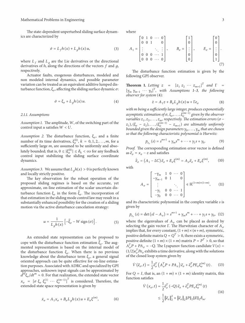
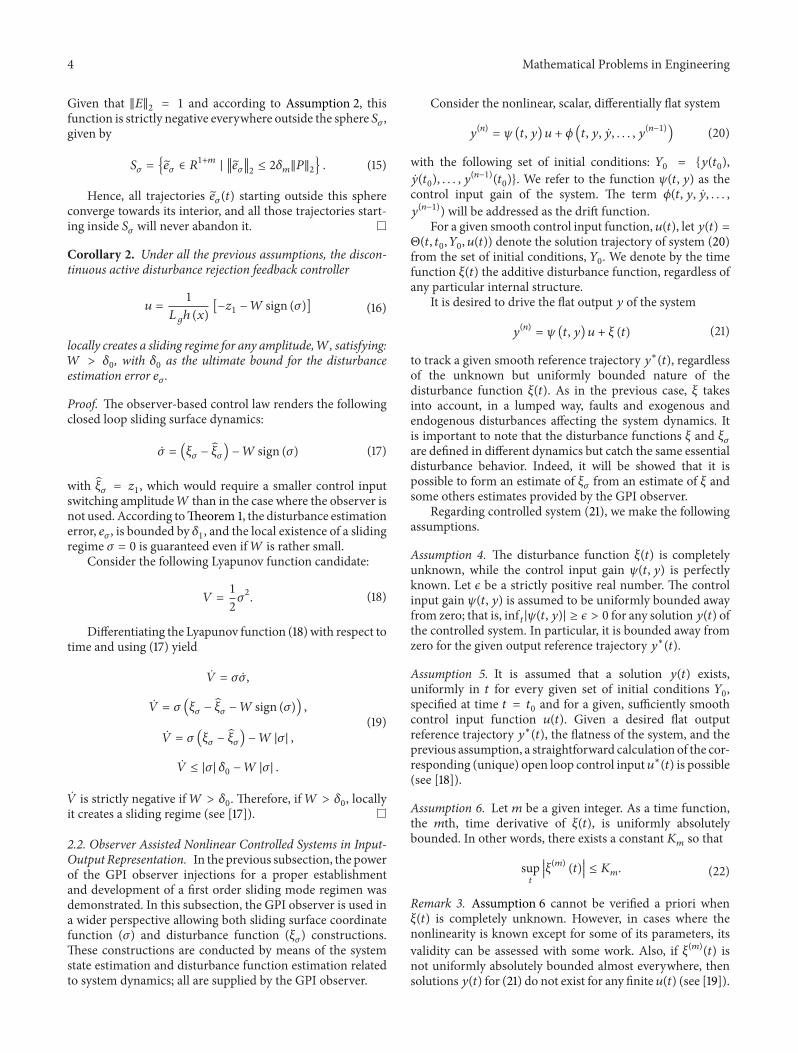
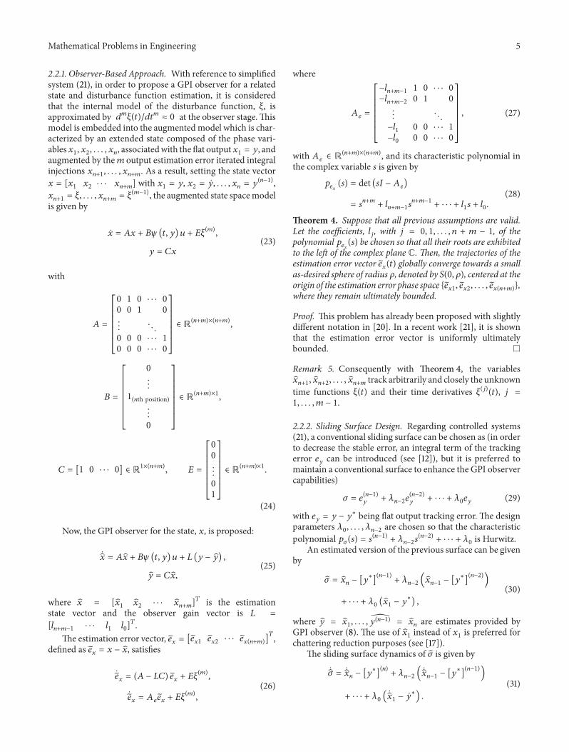
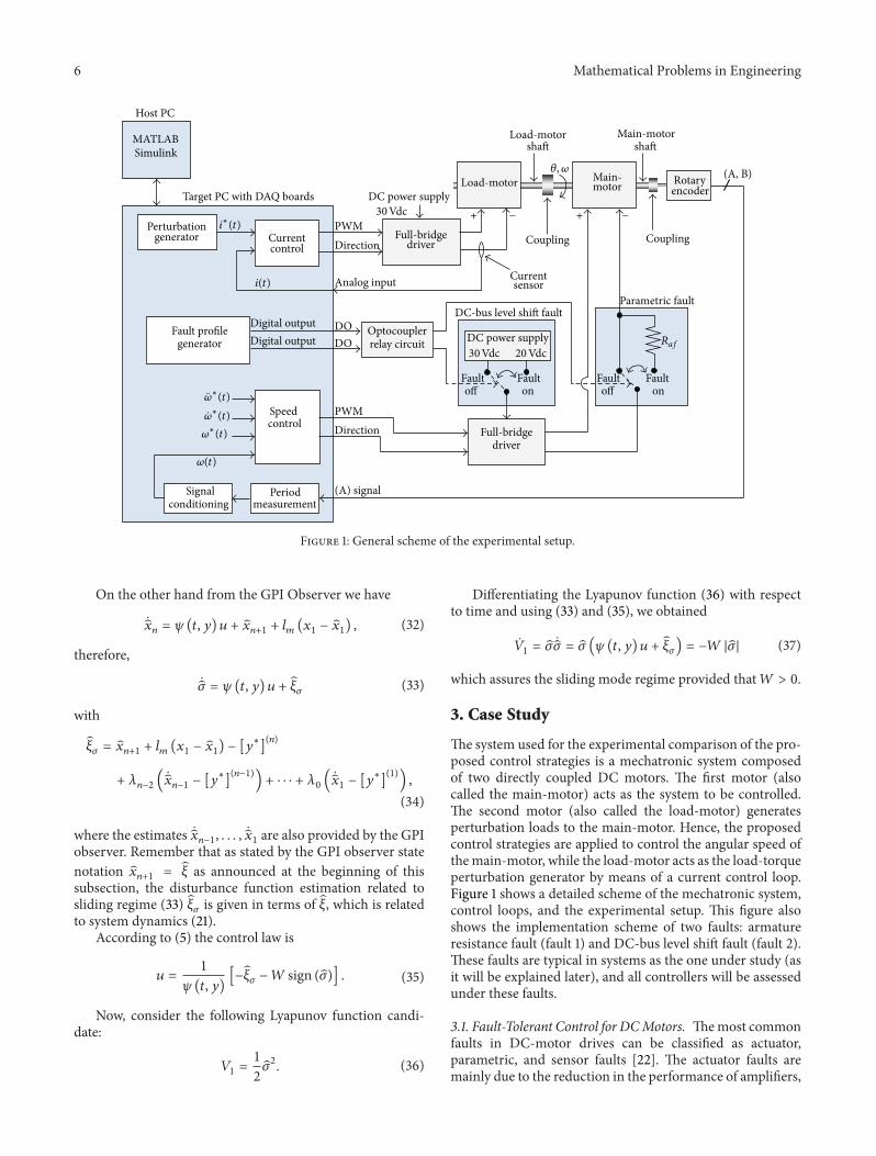
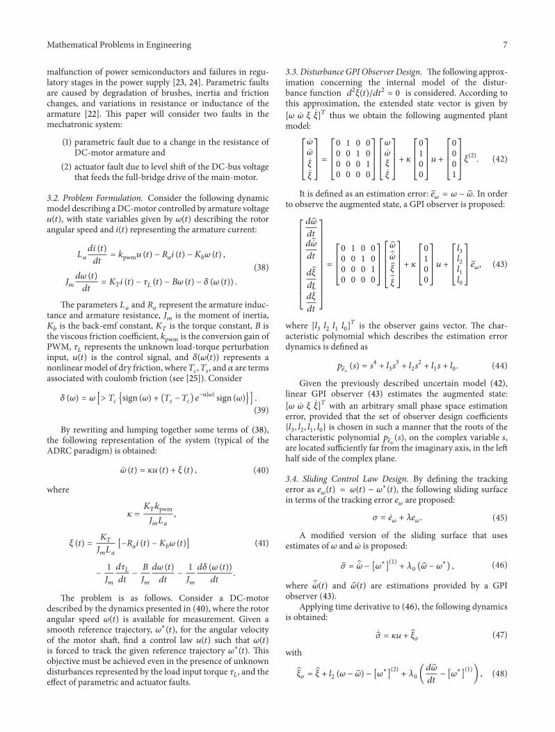
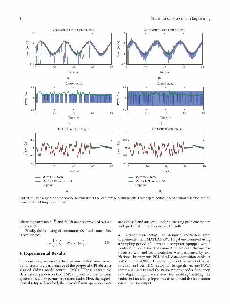
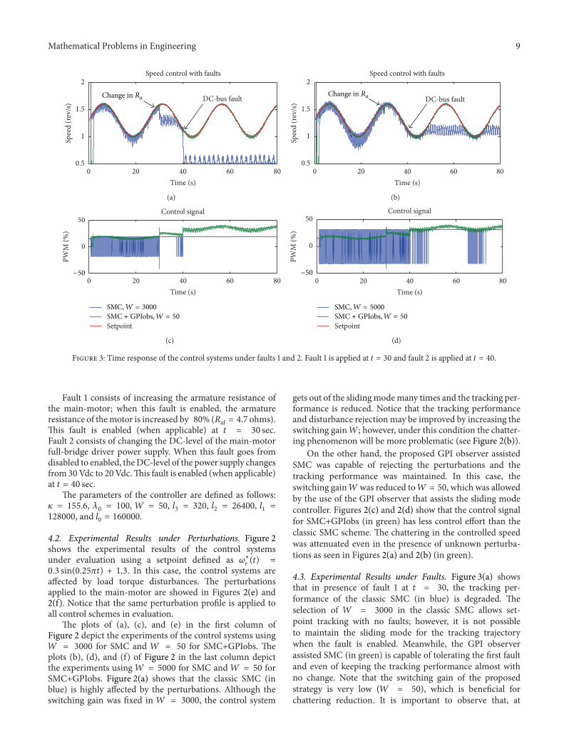
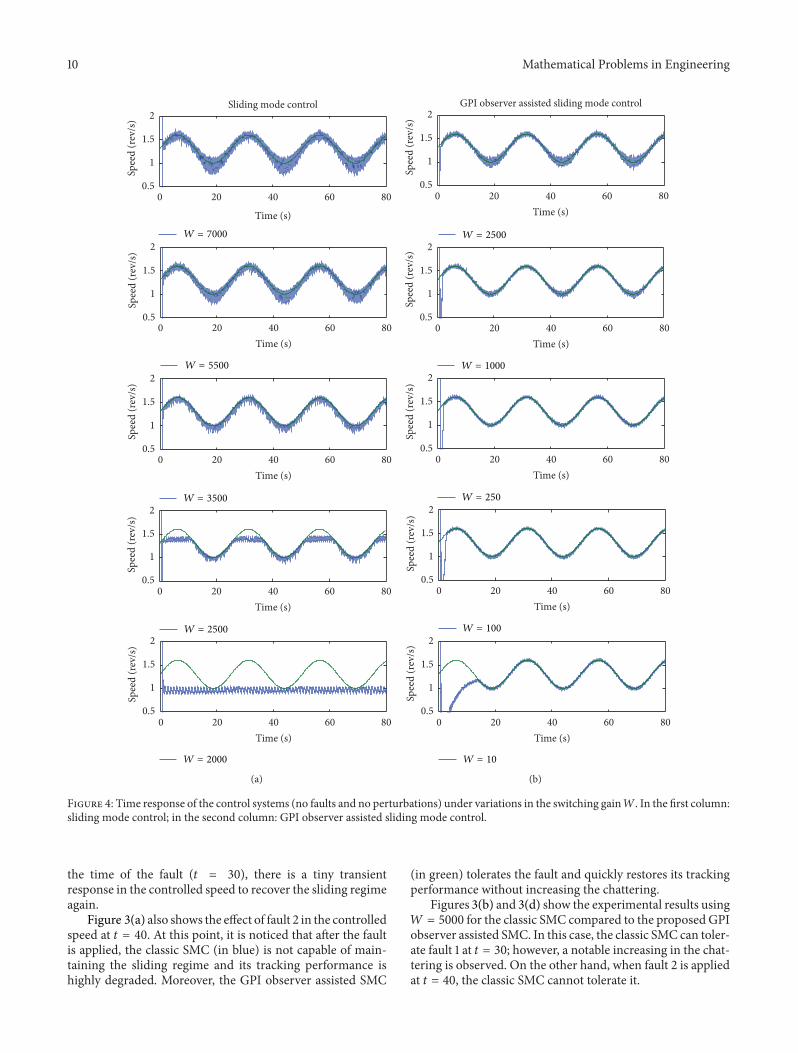


