Acoustic Scattering in Sheared Flow

David Iain Baker

Supervisor: Professor Nigel Peake

Department of Applied Mathematics and Theoretical Physics

University of Cambridge

This dissertation is submitted for the degree of

Doctor of Philosophy

St. Catharine’s College April 2019

Declaration

This dissertation is the result of my own work and includes nothing which is the outcome

of work done in collaboration except as declared in the Preface and specified in the text.

It is not substantially the same as any that I have submitted, or, is being concurrently

submitted for a degree or diploma or other qualification at the University of Cambridge or

any other University or similar institution except as declared in the Preface and specified

in the text. I further state that no substantial part of my dissertation has already been

submitted, or, is being concurrently submitted for any such degree, diploma or other

qualification at the University of Cambridge or any other University or similar institution

except as declared in the Preface and specified in the text.

David Iain Baker

April 2019

Acknowledgements

The work contained within the thesis would not have been possible without the assistance,

patience and support of friends, family and colleagues over the past four years.

Firstly, thanks must be given to my supervisor, Prof. Nigel Peake, for his guidance

and direction, both when work was going well and during more difficult phases of my

research, and the provision of the final encouragement needed to pull everything together.

His contributions were supported by presentations to and work with all members of the

Waves Group here in DAMTP: my contemporaries Owen and Peter (to whom I hope I

was a bearable officemate); and the experience of Lorna, Ed, Anastasia, James and James,

Ridhwaan, Doran and Stephen, who could draw on their work to enhance my own. Also,

the inspiration of the fresh younger faces of the Waves Group in Matthew, Chris, Georg

and Mungo, made the final stages of my thesis the most enjoyable of the entire process.

Finally, I would like to mention the contributions and discussions with William Devenport

and Ian Clark of Virginia Tech, who gave me the confidence that I could contribute to the

field.

Beyond the academic support of the group, the support of friends and family, both

within Cambridge and beyond, have been critical for keeping me working away. My

parents, for always giving me a place to get away and being two friends always willing to

talk; my brother for leading the way in his own work and ensuring I left my house from

time to time. To Sid and Simon and Anthony, for not getting fed up of my temperamental

hours and for making a home a pleasure to return to after a tough day of work.

And to Lizzie, who saw both the worst and the best, and somehow hasn’t run away

quite yet.

Further, I should like to the thank DAMTP and EPSRC for hosting and funding my

research, and to St. Catharine’s College for providing me a home and a place to belong for

the past eight years.

Finally, many thanks to Prof. Sjoerd Rienstra and Dr. Anurag Agarwal for examining

this thesis, providing both vital feedback and an opportunity to discuss the work within.

Abstract

Airframe noise, the noise of an aircraft in flight not due to the engine or other mechanical

devices, is often a major contribution to the sound heard from an aircraft during landing

approach. Over the past few decades certification requirements have gradually tightened,

reaching the point where the required noise reductions cannot be achieved through

reducing engine noise alone. There are, similarly, restrictions on the noise output of wind

turbines to reduce their impacts on local communities and wildlife. In practice this is

achieved by braking the turbines at high speed, reducing energy outputs and efficiency.

For both aircraft wings and turbine blades, the sharp trailing-edge is a well-understood

and unavoidable source of noise, scattering vortical, hydrodynamic disturbances within

the boundary-layer into far-field, acoustic, noise.

Inspired by nature, for example the silent flight of owls, modification of the flow

within the boundary-layer near the trailing-edge, either through passive or active devices,

appears to offer methods of reducing far-field noise. The precise mechanisms are not

completely understood, and this work focuses on the effect of varying boundary-layer

parameters near the trailing-edge on the resulting far-field noise. Alternative methods

of noise reduction include the addition of linings, for example via arrays of Helmholtz

resonators. The junctions at the leading- and trailing-edges of such linings can again be a

source of far-field noise, through a similar mechanism to that of a trailing-edge.

This scattering is analysed within a simplified mathematical framework through an

application of Rapid Distortion Theory, considering linearised perturbations to a trans-

versely sheared background flow. Within this framework, the development of disturbances

within a boundary-layer are investigated, both hydrodynamic and acoustic, over a variety

of mixed boundary conditions. The inclusion of background shear requires numerical

solution of differential equations, which are paired with complex variable techniques such

as the Wiener-Hopf method, constructed for the solution of boundary-value problems

with discontinuous boundary conditions. The possibility of exact solutions using this

technique allows asymptotic methods to be used to directly evaluate far-field noise.

Table of contents

Nomenclature xv

1 Introduction 1

1.1 Trailing-edge noise: generation and control . . . . . . . . . . . . . . . . . . . 1

1.1.1 Airframe noise . . . . . . . . . . . . . . . . . . . . . . . . . . . . . . . . . 1

1.1.2 Trailing-edge noise control . . . . . . . . . . . . . . . . . . . . . . . . . 2

1.1.3 Vortex sound models . . . . . . . . . . . . . . . . . . . . . . . . . . . . . 4

1.1.4 Rapid Distortion Theory . . . . . . . . . . . . . . . . . . . . . . . . . . . 6

1.1.5 Scattering . . . . . . . . . . . . . . . . . . . . . . . . . . . . . . . . . . . 8

1.1.6 Acoustic linings . . . . . . . . . . . . . . . . . . . . . . . . . . . . . . . . 10

1.2 Thesis structure . . . . . . . . . . . . . . . . . . . . . . . . . . . . . . . . . . . . 11

1.3 Summary of aims and objectives . . . . . . . . . . . . . . . . . . . . . . . . . . 15

2 Mathematical formulation of Rapid Distortion Theory 17

2.1 Basic concepts . . . . . . . . . . . . . . . . . . . . . . . . . . . . . . . . . . . . . 17

2.1.1 Equations of fluid dynamics . . . . . . . . . . . . . . . . . . . . . . . . 17

2.1.2 Mathematical conventions . . . . . . . . . . . . . . . . . . . . . . . . . 20

2.2 A wave equation for pressure . . . . . . . . . . . . . . . . . . . . . . . . . . . . 25

2.2.1 Assumptions . . . . . . . . . . . . . . . . . . . . . . . . . . . . . . . . . . 26

2.2.2 Compressible Rayleigh’s equation . . . . . . . . . . . . . . . . . . . . . 27

2.3 The adjoint problem for general continuous background profile . . . . . . . 30

2.4 Streamwise-homogeneous boundary conditions . . . . . . . . . . . . . . . . 33

3 Long-wavelength disturbances to piecewise-linear background flow 37

3.1 Introduction . . . . . . . . . . . . . . . . . . . . . . . . . . . . . . . . . . . . . . 37

3.2 Rapid Distortion Theory in the long-wavelength limit . . . . . . . . . . . . . 39

3.2.1 Outer region . . . . . . . . . . . . . . . . . . . . . . . . . . . . . . . . . . 40

3.2.2 Inner region . . . . . . . . . . . . . . . . . . . . . . . . . . . . . . . . . . 41

3.2.3 Alternative derivation of the equation in the inner region . . . . . . . 42

x Table of contents

3.2.4 Linear shear . . . . . . . . . . . . . . . . . . . . . . . . . . . . . . . . . . 43

3.3 Analytic solutions in the long-wavelength limit . . . . . . . . . . . . . . . . . 45

3.3.1 Matching at shear junctions . . . . . . . . . . . . . . . . . . . . . . . . . 48

3.3.2 Streamfunction for generic N -piece profile . . . . . . . . . . . . . . . . 49

3.4 A point source in sheared flow . . . . . . . . . . . . . . . . . . . . . . . . . . . 53

3.4.1 Fixed mass or momentum source: Setup . . . . . . . . . . . . . . . . . 54

3.4.2 Auxiliary functions and the general solution for arbitrary (linear)

boundary conditions . . . . . . . . . . . . . . . . . . . . . . . . . . . . . 56

3.4.3 Preliminaries: towards an analytic solution . . . . . . . . . . . . . . . . 58

3.4.4 Explicit choice of piecewise linear background profiles . . . . . . . . . 60

3.5 Fixed mass or momentum source: Hard-wall . . . . . . . . . . . . . . . . . . . 62

3.5.1 The dispersion function . . . . . . . . . . . . . . . . . . . . . . . . . . . 63

3.5.2 Fourier inversion . . . . . . . . . . . . . . . . . . . . . . . . . . . . . . . 65

3.5.3 Branch cut contribution: Matching to radiating acoustic outer solution 67

3.5.4 Modal solutions . . . . . . . . . . . . . . . . . . . . . . . . . . . . . . . . 72

3.5.5 Variation of internal shear . . . . . . . . . . . . . . . . . . . . . . . . . . 74

3.6 Lined walls: pressure-release and impedance conditions . . . . . . . . . . . 78

3.6.1 Quantity of pressure-release modes . . . . . . . . . . . . . . . . . . . . 80

3.6.2 Stability of pressure-release modes . . . . . . . . . . . . . . . . . . . . 83

3.6.3 Impedance modes . . . . . . . . . . . . . . . . . . . . . . . . . . . . . . 86

3.6.4 Far-field noise . . . . . . . . . . . . . . . . . . . . . . . . . . . . . . . . . 89

3.7 Fixed mass or momentum source: Wake . . . . . . . . . . . . . . . . . . . . . 91

3.7.1 Simplification in the symmetric case . . . . . . . . . . . . . . . . . . . 93

3.8 Discussion and conclusions . . . . . . . . . . . . . . . . . . . . . . . . . . . . . 96

4 Disturbances to continuously sheared flow above a homogeneous boundary 99

4.1 Introduction . . . . . . . . . . . . . . . . . . . . . . . . . . . . . . . . . . . . . . 99

4.2 Solving the adjoint compressible Rayleigh equation . . . . . . . . . . . . . . . 101

4.2.1 Preliminaries . . . . . . . . . . . . . . . . . . . . . . . . . . . . . . . . . 102

4.2.2 Analytic solution: Uniform flow . . . . . . . . . . . . . . . . . . . . . . 104

4.2.3 Numerical solution: Integration across boundary-layer . . . . . . . . 105

4.2.4 Numerical solution: Integration across "complex" boundary-layer . . 109

4.2.5 Asymptotic solution: High frequency acoustics . . . . . . . . . . . . . 114

4.3 A point mass source in continuous shear . . . . . . . . . . . . . . . . . . . . . 118

4.3.1 Far-field noise: Steepest descent . . . . . . . . . . . . . . . . . . . . . . 120

4.4 Hard-wall boundaries . . . . . . . . . . . . . . . . . . . . . . . . . . . . . . . . 125

4.4.1 Integrated near-field solutions . . . . . . . . . . . . . . . . . . . . . . . 127

Table of contents xi

4.4.2 Far-field sound: outside shear layer . . . . . . . . . . . . . . . . . . . . 127

4.4.3 Far-field sound: downstream of source . . . . . . . . . . . . . . . . . . 136

4.5 Pressure-release and impedance boundaries . . . . . . . . . . . . . . . . . . . 138

4.5.1 Pressure-release conditions . . . . . . . . . . . . . . . . . . . . . . . . . 139

4.5.2 General impedance boundary condition . . . . . . . . . . . . . . . . . 142

4.6 Wake solutions . . . . . . . . . . . . . . . . . . . . . . . . . . . . . . . . . . . . 146

4.6.1 Auxiliary functions . . . . . . . . . . . . . . . . . . . . . . . . . . . . . . 146

4.6.2 Complete inversion . . . . . . . . . . . . . . . . . . . . . . . . . . . . . . 150

4.6.3 Far-field noise . . . . . . . . . . . . . . . . . . . . . . . . . . . . . . . . . 151

4.7 Discussion and conclusions . . . . . . . . . . . . . . . . . . . . . . . . . . . . . 157

5 Scattering from a junction 159

5.1 Introduction . . . . . . . . . . . . . . . . . . . . . . . . . . . . . . . . . . . . . . 159

5.2 The generic scattering problem . . . . . . . . . . . . . . . . . . . . . . . . . . . 161

5.2.1 Half-range Fourier transforms and the Wiener-Hopf method . . . . . 162

5.2.2 Explicit computation of splitfunctions . . . . . . . . . . . . . . . . . . 165

5.2.3 Generalised half-planes . . . . . . . . . . . . . . . . . . . . . . . . . . . 169

5.2.4 Numerical computation of splitfunctions . . . . . . . . . . . . . . . . . 170

5.2.5 Multiplicative factorisation: Winding numbers, continuity of log and

curved branch cuts . . . . . . . . . . . . . . . . . . . . . . . . . . . . . . 170

5.2.6 Linking small x1 and large k1 behaviour . . . . . . . . . . . . . . . . . . 172

5.3 Slipping sheared flow: Hard-soft transition . . . . . . . . . . . . . . . . . . . . 173

5.3.1 Problem setup and incident field . . . . . . . . . . . . . . . . . . . . . . 173

5.3.2 The Wiener-Hopf kernel and factorisation . . . . . . . . . . . . . . . . 175

5.3.3 Numerical inversion . . . . . . . . . . . . . . . . . . . . . . . . . . . . . 180

5.3.4 Far-field noise . . . . . . . . . . . . . . . . . . . . . . . . . . . . . . . . . 182

5.4 Non-slipping sheared flow: Hard-soft transition . . . . . . . . . . . . . . . . . 190

5.4.1 Far-field kernel . . . . . . . . . . . . . . . . . . . . . . . . . . . . . . . . 190

5.4.2 Numerical inversion . . . . . . . . . . . . . . . . . . . . . . . . . . . . . 191

5.4.3 Behaviour of scattered solution near the junction . . . . . . . . . . . . 196

5.4.4 Far-field noise . . . . . . . . . . . . . . . . . . . . . . . . . . . . . . . . . 197

5.4.5 The consistency of the no-slip limit . . . . . . . . . . . . . . . . . . . . 197

5.4.6 The incompressible (long-wavelength) limit . . . . . . . . . . . . . . . 197

5.5 Transition between two different lined surfaces . . . . . . . . . . . . . . . . . 200

5.5.1 Soft to hard transition . . . . . . . . . . . . . . . . . . . . . . . . . . . . 200

5.5.2 Impedance to impedance transition . . . . . . . . . . . . . . . . . . . . 200

5.6 Restabilisation of unstable modes . . . . . . . . . . . . . . . . . . . . . . . . . 203

xii Table of contents

5.6.1 Restabilisation of an unstable mode . . . . . . . . . . . . . . . . . . . . 205

5.6.2 Finite unstable lining . . . . . . . . . . . . . . . . . . . . . . . . . . . . . 206

5.7 Discussion and conclusions . . . . . . . . . . . . . . . . . . . . . . . . . . . . . 210

6 Scattering from a sharp trailing-edge 215

6.1 Introduction . . . . . . . . . . . . . . . . . . . . . . . . . . . . . . . . . . . . . . 215

6.2 Scattering from a generic trailing-edge . . . . . . . . . . . . . . . . . . . . . . 217

6.2.1 Scattering from a generic, harmonic, incident field . . . . . . . . . . . 217

6.2.2 The Green’s function: incident vortex sheet . . . . . . . . . . . . . . . . 221

6.2.3 Simplification in the symmetric case . . . . . . . . . . . . . . . . . . . 223

6.2.4 Kernel far-field behaviour and factorisation . . . . . . . . . . . . . . . 223

6.2.5 Near- and far-field inversion for g (s) . . . . . . . . . . . . . . . . . . . . 226

6.3 Distributed boundary-layer vorticity . . . . . . . . . . . . . . . . . . . . . . . . 231

6.3.1 Numerical solutions . . . . . . . . . . . . . . . . . . . . . . . . . . . . . 233

6.4 Analysis of noise-reduction hypotheses . . . . . . . . . . . . . . . . . . . . . . 236

6.4.1 Modification of the transfer function by shear layer . . . . . . . . . . . 237

6.4.2 Reduction of wall pressure by vorticity displacement . . . . . . . . . . 238

6.4.3 Wall-pressure and far-field noise prediction from a physically moti-

vated boundary-layer . . . . . . . . . . . . . . . . . . . . . . . . . . . . 242

6.5 Conclusions and discussion . . . . . . . . . . . . . . . . . . . . . . . . . . . . . 245

7 Conclusions 247

7.1 Summary and discussion . . . . . . . . . . . . . . . . . . . . . . . . . . . . . . 247

7.1.1 Implementation of quasi-numerical methods . . . . . . . . . . . . . . 247

7.1.2 Development of the understanding of scattering problems . . . . . . 248

7.1.3 Explaining noise control devices . . . . . . . . . . . . . . . . . . . . . . 249

7.2 Future work . . . . . . . . . . . . . . . . . . . . . . . . . . . . . . . . . . . . . . 251

References 253

Appendix A Appendices to Chapter 3 263

A.1 The existence N hard-wall modes . . . . . . . . . . . . . . . . . . . . . . . . . 263

A.2 Numerical complex methods implementation . . . . . . . . . . . . . . . . . . 264

A.2.1 Integration . . . . . . . . . . . . . . . . . . . . . . . . . . . . . . . . . . . 264

A.2.2 Pole/zero finding . . . . . . . . . . . . . . . . . . . . . . . . . . . . . . . 265

Appendix B Appendix to Chapter 4 269

B.1 Numerical solution: Frobenius methods . . . . . . . . . . . . . . . . . . . . . 269

Table of contents xiii

B.1.1 Computation of Taylor/Laurent coefficients . . . . . . . . . . . . . . . 271

B.1.2 Construction of ODE solutions, and range of validity . . . . . . . . . . 272

Nomenclature

Acronyms / Abbreviations

gLHzP Generalised Lower Half z-plane

gUHzP Generalised Uper Half z-plane

LHzP Complex Lower Half z-plane

RDB Rienstra, Darau and Brambley 2013 [92]

RDT Rapid Distortion Theory

UHzP Complex Upper Half z-plane

Subscripts

·0 Mean flow quantity (in derivation)

Temporally Fourier transformed quantity

·1 In §6, typically a function or operator evaluated for x2 < 0 or as

x2 → 0− (where it cannot be confused with Fourier transforms)

·2 In §6, typically a function or operator evaluated for x2 < 0 or as

x2 → 0− (where it cannot be confused with Fourier transforms)

·ℓ A quantity generated from boundary conditions given by generic

linear operator L

·≷ If x2 > y2, this function is the decaying auxiliary function ·d , else

it is the auxiliary function satisfying the boundary condition on

x2 = 0 or as x2 →−∞

·∞ Variable evaluated in free-stream, x2 > δ, or in limit x2 →∞

xvi Nomenclature

·± Multiplicative factorisation of a function, analytic and nonzero in

the relevant half-plane

In §3, a quantity that is either exponentially decaying or growing as

x2 →∞, typically derived from the normalised streamfunction

·a In derivation in §3, acoustic (outer) variables

·b In derivation in §3, boundary-layer (inner) variables

·d A quantity which decays exponentially as x2 →∞

·h A quantity generated from boundary conditions given by wall-

normal velocity operator V

· j , j = 1,2,3 Spatially Fourier transformed quantity

·p A quantity generated from boundary conditions given by pressure

operator P

·S Function evaluated at at saddle point of far-field exponent f or F

·T = (·2, ·3) Components of three-dimensional vector field in transverse direc-

tion to mean flow

·computed The relevant function computed using a Runge-Kutta routine

·frobenius The relevant function computed using a Frobenius method

·incompressible The relevant function in the incompressible c0 →∞ limit

·BC Part of Fourier inversion with contributions only from branch cut

contours CU and CL

·C L The component of a function computed by Fourier inversion around

the critical-layer branch cut only

·m j Disturbances due to scattering of j th mode

Caligraphic (Roman) symbols and differential operators

Di The incompressible Rayleigh operator, applied to streamfunction

perturbations

Nomenclature xvii

D0

DtThe mean-flow material derivative,

∂

∂t+U

∂

∂x1

for parallel mean

flow

D

DtThe material derivative,

∂

∂t+u·∇ governing the change of a quantity

moving with the fluid

ℓ Streamwise distance between generation of surface modes and the

stabilising junction

D Generic linear differential operator

D†R The adjoint compressible Rayleigh operator, defined by (2.3.11)

Di The incompressible Rayleigh operator, applied to pressure pertur-

bations

DR The compressible Rayleigh operator, defined by (2.3.12)

L Spanwise correlation lengthscale in Amiet’s equation, (1.1.1)

LZ The impedance operator, typically the combination iωZV−CP

P Operator, when applied to perturbation potential returns the pres-

sure perturbation p ′

V Operator, when applied to perturbation potential returns the wall-

normal velocity perturbation v ′

∂i Shorthand for spatial partial derivative, ∂/∂xi

Greek Symbols

α The ratio between the wall background shear and frequency, α=ω/σ

Complex exponent useful in factorising far-field Wiener-Hopf ker-

nel

β Scaling of coordinates by large free-stream Mach number, β2 =1−M 2∞

χ2 Typically an arbitrary value of x2, such as the location of a jump in

background shear

xviii Nomenclature

δx2 Integration step-size for Runge-Kutta routines

∆ A quantity governing the relationship in the jump of perturbation

wall-normal velocity and pressure across a jump in background

shear, defined via (3.3.11)

δ As a function, the Dirac-δ function

Boundary-layer thickness, typical boundary-layer for x2 ∈ (0,δ)

δ± Boundary-layer thickness for x2 ≷ 0, respectively

δ j Intermediate location within boundary-layer, typically for piecewise-

linear profiles

ϵ In §3, small quantity ϵ= k0δ when the boundary-layer is acousti-

cally compact

In §4.2.5, the small parameter k−11

η (Perturbation) particle displacement, typically around a vortex

sheet

Γ In §4.2.5, the acoustic exponent γ scaled by small parameter ϵ

γ Acoustic exponent defined by (4.2.12)

Ratio of specific heat capacities, γ= cp /cV

A simple closed contour containing the point z = 0, in §B.1

κ The incompressible limit of γ, namely√

k21 +k2

3 , with branch cuts

as defined by figure 3.3.1

κ1 The convection wavenumber of a disturbance moving at the back-

ground velocity Uc , with κ1 =ω/Uc

κh j Wavenumber of j th hard-wall mode

κp j Wavenumber of j th pressure mode

λ Disturbance wavelength, 2π/k

µ Dynamic viscosity of fluid

Complex number quantifying the behaviour of a Wiener-Hopf ker-

nel as z →−∞

Nomenclature xix

ν Kinematic viscosity of fluid, µ/ρ

Complex number quantifying the behaviour of a Wiener-Hopf ker-

nel as z →+∞

Ω In §4.2.5, the frequency ω scaled by small parameter ϵ

ω (Angular) frequency of disturbance

Φ In §4.2.5, scaled φ satisfying the canonical WKBJ equation

φ Acoustic velocity potential (non-sheared background flow)

Generalised velocity potential (sheared background flow)

φ∗ Trailing-edge potential appearing in far-field Green’s function in

vortex sound models

Ψ Streamwise Fourier transform of perturbation streamfunction,Ψ=ψ01.

ψ Streamfunction for two-dimensional, incompressible flow

ρ Fluid density

σ The background shear within an intermediate boundary-layer in-

terval I j

σ± Real constants defining the strip of analyticity for computing Wiener-

Hopf factorisations

σ1,2 In §B.1, two roots of the indicial equation

Otherwise, the background shear respectively for x2 = 0±

τ Source time

Θ Mach-scaled observer angle, tanΘ=βx2/x1, in §4.3.1

θ The observer angle, θ = tan−1(x2/x1)

ω The vorticity of a fluid,ω=∇×u. If flow is two dimensional,ω=ω3

(not to be confused with angular frequency).

Φ Some vector representation of potential φ, satisfying a first-order

(multidimensional) differential equation. Typically Φ1 = φ and

Φ2 =φ′

xx Nomenclature

σ Deviatoric stress tensor

Dimensionless Numbers

Ma Mach number, U /c0

Re Reynolds number of flow, (2.1.3).

Superscripts

·′ Perturbation quantity

·1 In §6, typically a function or operator evaluated for x2 > 0 or as

x2 → 0+ (when confusion with Fourier transforms might arise)

·2 In §6, typically a function or operator evaluated for x2 < 0 or as

x2 → 0− when confusion with Fourier transforms might arise)

·d Downstream operator or dispersion function, typically defined on

x1 > 0

·u Upstream operator or dispersion function, typically defined on

x1 < 0

·(i ) Incident disturbance in scattering problems, §5 and §6

·(s) Incident disturbance in scattering problems, §5 and §6

·(s1) Component of a solution scattered by the first junction

·(s2) Component of a solution scattered by the second junction

·± Coupled with subscript ·1, half-range streamwise Fourier trans-

form as defined by (5.2.2a). Equivalent to additive factorisation of

streamwise Fourier transform

Additive factorisation of function, analytic in the relevant in the

relevant half plane

A function analytic in the relevant upper/lower half plane

·± Typically the background flow field, defined by U (x2) = ±U±(x2)

for x2 ≷ 0

Roman Symbols

Nomenclature xxi

F Integrated boundary-layer quantity, governing the scattering of

convected quantity F

K Wiener-Hopf kernel normalised by large k1 behaviour K = K /K f

D0 Shorthand for mean-flow material derivative operator D0/Dt

i Imaginary unit, i 2 =−1

λa The acoustic wavelength, 2π/k0 = 2πc0/ω

λh The hydrodynamic wavelength, 2π/κ1 = 2πU (y2)/ω

ωc Generalised convected vorticity

C Unknown convected quantity, with no direct effect on governing

acoustic behaviour

e Strain rate tensor

F Vector representation of the adjoint Rayleigh equation, as per (4.2.15)

f Additional force source term

k = (k1,k2,k3) Spatial wavenumbers

M j Matrices ( j = 1,2) arising in the derivation of the jump of perturba-

tion variables across a junction in background shear in §3

S j Matrices ( j = 1,2) linking the coefficients of growing and decaying

terms across a jump in background shear, in §3

u = (u, v, w) Velocity field of fluid

x = (x1, x2, x3) Spatial location

Observer location

y = (y1, y2, y3) Source location

A The coefficient of auxiliary function φd in the scattering problem

b Aerofoil spanlength in Amiet’s equation, (1.1.1)

B+ Unknown continuation of downstream boundary condition on

upstream boundary in §5

xxii Nomenclature

C Streamwise Fourier-transformed, time-harmonic, convective deriva-

tive, C (x2) = i (ω−U (x2)k1)

In §4 and thereafter, a complex integration contour in z-space for

solution of the governing ODE

In §5 and §6, a generic separation contour, C =C+ or C =C−

c Aerofoil chordlength in Amiet’s equation, (1.1.1)

Dimensionless speed of sound, in derivation in §3

C ′ Wall-normal derivative of C , C ′(x2) =−iU ′(x2)k1

C− Unknown continuation of upstream boundary condition on down-

stream boundary in §5

c0 Speed of sound

cn In §B.1, the coefficients of the power series expansion of first, non-

logarithmic solution φ1

cp Specific heat of fluid, at constant pressure

cV Specific heat of fluid, at constant volume

C± Wiener-Hopf separation contour used in the Cauchy integral for

additive factorisations

CU ,L Fourier inversion contours, rays in the complex k1-plane making

an angle π/2−θ to the real axis, where θ is the observer angle

D The dispersion function for some given boundary conditions, with

dispersion relation D(k1,ω) = 0 giving the location of modal solu-

tions

In §B.1, the coefficient of the logarithmic term in second solution

φ2

dn In §B.1, the coefficients of non-logarithmic part of the second solu-

tion φ2

E An entire function of its complex argument

F Combined force and mass source for a long-wavelength distur-

bance

Mach-scaled exponent of far-field Fourier inversion integral, (4.3.18)

Nomenclature xxiii

f Exponent of far-field Fourier inversion integral, (4.3.15)

F j Spatial inversion contour for wavenumber k j .

g Green’s function for the adjoint Rayleigh operator with upstream

exp(iκ1x1) dependence

GR Green’s function for the direct Rayleigh operator, DR

G†R Green’s function for the adjoint Rayleigh operator, D†

R

H Heaviside function, 1 for positive argument, 0 otherwise

H (2)n Hankel function of the second kind, of order n, equal to Jn − i Yn

I+ The downstream half-range transform of the incident disturbance

φ(i )

Iℓ The kernel of the Fourier inversion for boundary operator L, in

the piecewise-linear point source problem §3.4.1 and the reduced

kernel in §4.3.1

I j An intermediate boundary-layer interval, I j = [δ j ,δ j+1)

I+p Half-range Fourier transform of pressure due to incident distur-

bance on the wake of a trailing-edge

I+v Half-range Fourier transform of vertical velocity due to incident

disturbance on the wake of a trailing-edge

IF F The directivity of the radiated far-field noise

Jn Bessel function of the first kind, of order n

K Wiener-Hopf kernel

K ∗ Particularly in §6, the scattering kernel with iωZ terms removed

K0 Mach-scaled far-field acoustic wavenumber, incorporating cross-

stream effects, (4.3.16b)

k0 Acoustic wavenumber, ω/c0

K1 Mach-scaled far-field streamwise wavenumber, (4.3.16a)

xxiv Nomenclature

Ki In §4.2.5, the wavenumber ki scaled by small parameter ϵ

k1 j The streamwise wavenumber of the j th modal solution

K1SD The (Mach-scaled) steepest-descent contour outside the boundary-

layer

K f Approximation to the Wiener-Hopf kernel for large k1, particular

when k1 is real

L Typical lengthscale for flow

Lω Temporal inversion contour (for Briggs-Bers inversion)

lp Spanwise correlation lengthscale in Amiet’s equation, (1.1.1)

M j Strength of j th modal contribution

N The number of piecewise-linear line segments in the background

profile

The number of integration points in in the Runge-Kutta routines

N∞ Some large number of integration points in the Runge-Kutta rou-

tines, for reference, chosen to be 105

Nh Number of hard-wall modes

NP The number of poles of a complex function within a defined con-

tour

Np Number of pressure-release modes

NZ The number of zeros of a complex function within a defined con-

tour

P In §B.1, the coefficient of φ′, p, with a pole at the regular singular

point factored out

p Pressure field of fluid

Where clear, the coefficient of φ′ in the triply-transformed adjoint

Rayleigh equation, (4.2.22)

pn In §B.1, the coefficients of the power series expansion of P

Nomenclature xxv

pw Pressure perturbation evaluated at x2 = 0

Q Generalisation of point mass source strength q0 to include effect of

background flow and shear

In §B.1, the coefficient of φ, q , with a double pole at the regular

singular point factored out

q Additional mass source term

Where clear, the coefficient of φ′ in the triply-transformed adjoint

Rayleigh equation, (4.2.22)

q0 Strength of a point mass source

qn In §B.1, the coefficients of the power series expansion of Q

R A polynomial use to remove poles of dispersion functions, defined

in (3.5.4)

re Distance of observer from source, modified for Doppler effect

S Generic source term for Briggs-Bers analysis

s Entropy field of fluid

S j For j = 0,1, . . . , the coefficients of the Liouville-Green expansion of

Φ in the WKBJ analysis in §4.2.5

Spp Spectral pressure density

T Dimensionless time variable, in derivation in §3

t Temporal location, time

U Streamwise component of parallel mean flow profile

Typical velocity scale for flow

U∗ If parallel mean flow U (x2) is defined for x2 < 0, U∗(x2) =U (−x2)

U± Functions unknown save for their complex analyticity

Uc Convection velocity of gust disturbance

U j Intermediate background velocity within boundary-layer, typically

for piecewise-linear profiles

xxvi Nomenclature

W The Wronskian of two linearly independent solutions of an ordinary

differential equation

W0 Representative value of Wronskian evaluated at a specific point

Wn The Lambert-W or product log function, nth branch

Xi Dimensionless spatial variable, in derivation in §3

Yn Bessel function of the second kind, of order n

Z Impedance of a lined surface

z Complex representation of observer location, z = x1 + i x2

Analytic continuation of wall-normal coordinate x2 into the com-

plex plane, when integrating the governing ODE, provided U (x2)

permits analytic continuation

Other Symbols

[·]χ2 Jump in quantity across x2 =χ2

Chapter 1

Introduction

1.1 Trailing-edge noise: generation and control

1.1.1 Airframe noise

Understanding of the propagation and generation of small pressure perturbations in air

or water, perceived by the human ear as sound, is fundamental in controlling its impact

on day-to-day life. Noise generation has been studied within a mathematical framework

since Lighthill’s 1952 theory of aerodynamic sound [69, 70], which concerns itself with the

generation of acoustic noise from a region of turbulent flow. The resulting sound waves

propagate at a well-understood speed of sound (which depends on the medium), however

the generation of these waves is driven by chaotic breakdown of instabilities in viscous

shear flow.

As anybody who lives near an airport can attest, aircraft are noisy. A large proportion

of this noise is airframe noise: the noise of an aircraft in flight not due to the engine

and other propulsive devices [32]. Over the past few decades, certification requirements

(particularly with regards noise near airports) have gradually tightened to the point where

the required noise reductions cannot be achieved through reduction of engine noise alone.

A large component of airframe noise is related to wing flaps and landing gear, however

there is a large contribution from the sharp trailing-edge of the aerofoil. This trailing-edge

is a well understood and unavoidable source of noise. Vortical disturbances within a

turbulent boundary layer interact with the sharp trailing-edge of an aerofoil, with the

resulting broadband scattered pressure fluctuations propagating to the far-field as sound.

The sound intensity of this noise source scales with velocity as U 3Ma2 independently of

the behaviour of the unsteady flow [34], with Ma = U /c0 the flow Mach number. This

should be compared to the classical result of sound intensity of turbulence with no

2 Introduction

hard boundaries within the flow, scaling as U 3Ma5 [70]. Similar trailing-edge generated

noise arises in other contexts, in particular wind turbines. As with aircraft, there are

restrictions on the noise output of wind turbines so as to reduce their impacts on local

communities and wildlife [67]. In practice this is achieved by braking the turbines at high

speed, reducing energy outputs and efficiency.

1.1.2 Trailing-edge noise control

The sharp trailing-edge is necessary aerodynamically for lift, and hence controlling this

noise is difficult. With this in mind, a variety of noise-control devices have been proposed,

either through modification of the aerofoil geometry or by controlling the behaviour of

the turbulent flow near the trailing-edge. These two different broad forms of noise control

arise from fundamentally different mechamisms, illustrated by considering Amiet’s theory

of trailing-edge noise [5, 6], which links the spectrum of far-field sound (denoted here

Spp (x1, x2,0,ω) for observer location (x1, x2) at frequency ω) with the surface pressure

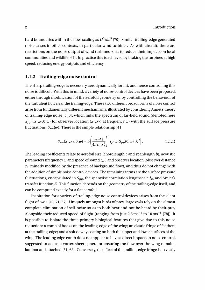
fluctuations, Spp (ω). There is the simple relationship [41]

Spp (x1, x2,0,ω) ≈ b

(ωcx2

4πc∞r 2e

)2

lp (ω)Spp (0,ω)∣∣∣L2

∣∣∣ . (1.1.1)

The leading coefficients relate to aerofoil size (chordlength c and spanlength b), acoustic

parameters (frequencyω and speed of sound c∞) and observer location (observer distance

re , minorly modified by the presence of background flow), and thus do not change with

the addition of simple noise control devices. The remaining terms are the surface pressure

fluctuations, encapsulated in Spp , the spanwise correlation lengthscale lp , and Amiet’s

transfer function L. This function depends on the geometry of the trailing-edge itself, and

can be computed exactly for a flat aerofoil.

Inspiration for a variety of trailing-edge noise control devices arises from the silent

flight of owls [49, 71, 37]. Uniquely amongst birds of prey, large owls rely on the almost

complete elimination of self-noise so as to both hear and not be heard by their prey.

Alongside their reduced speed of flight (ranging from just 2.5 ms−1 to 10 ms−1 [78]), it

is possible to isolate the three primary biological features that give rise to this noise

reduction: a comb of hooks on the leading-edge of the wing; an elastic fringe of feathers

at the trailing-edge; and a soft downy coating on both the upper and lower surfaces of the

wing. The leading edge comb does not appear to have a direct impact on noise control,

suggested to act as a vortex sheet generator ensuring the flow over the wing remains

laminar and attached [51, 68]. Conversely, the effect of the trailing-edge fringe is to vastly

1.1 Trailing-edge noise: generation and control 3

reduce the noise of the owl [71], though this alone cannot explain the entirety of the noise

reduction. This fringe has been modelled mathematically by Jaworski and Peake [63],

as a porous and elastic trailing-edge using the Wiener-Hopf technique, suggesting the

noise scales like U 3Ma3 as opposed to U 3Ma2 for a hard edge, particularly at medium

and higher frequencies (in this case above approximately 1.6 kHz, which corresponds to

an acoustic wavelength comparable to the observed minimal wing chord of silent owls

– smaller owls which don’t rely on being silent do not have the previous discussed wing

features).

A variety of trailing-edge control devices mimicking this behaviour have previously

been proposed and implemented. The use of serrated trailing-edges (both sawtooth

and sinusoidal) for noise reduction has been studied (with success) experimentally [65,

74] and mathematically [57, 72], and indeed has been applied to wind turbines in the

form of Siemens’ DinoTail [100]. With regards Amiet’s formula (1.1.1), these primarily

lead to modification of the transfer function L, as with porous and elastic trailing-edge

modifications (for example [99]), though the exact mechanism behind this varies.

Recent work by Clark et al. [28, 26, 25, 24] led to the development of finlets, streamwise-

oriented fence-like objects near, or upstream of, the trailing-edge, deriving inspiration

from fibres on the upper surface of the wing of a silent owl. Numerical and experimental

investigations of similar objects show a reduction in far-field noise resulting from trailing-

edge scattering [3, 4, 15]. Active noise control measures have also been proposed, typically

blowing or suction near the trailing-edge or into the wake, both constantly and periodically

[118, 36, 106]. These methods have the advantage of a far greater degree of control,

and thus applicability to a wider range of flow conditions. Common to both blowing

and the finlet or fence-like devices is the reduction in surface pressure fluctuations Spp ,

identified in (1.1.1) as the critical measurable quantity that is transferred to the far-field.

Further, the “cutting” effect of the fence-like structure is hypothesised to reduce the

spanwise correlation lengthscales lp . There are detailed measurements of boundary-layer

profile both for finlets and for near-edge blowing, both showing boundary-layer distortion

and a separation of the turbulent boundary-layer behind the device. Typically, hot-wire

measurements of the boundary-layer profile are used to measure the mean streamwise

flow velocity, and the root mean square of velocity perturbations, sometimes at a variety of

streamwise locations both upstream, above, and downstream of the noise control devices

[106]. Further, recent large eddy simulations [16] support both the argument of a reduction

in spanwise lengthscales through “chopping” of turbulent eddies, and a reduction in

surface pressure fluctuations through movement of eddies away from the hard surface.

Further numerical work, again supporting the argument of noise reduction through

4 Introduction

deflection of turbulence, includes some limited, two-dimensional RANS simulations [98],

though the two-dimensional setup limits the applicability of this investigation.

Whilst these devices broadly seem successful in the reduction of far-field noise, it is

worth noting a pair of caveats. Firstly, any noise control device must not have a large

effect on the aerodynamic characteristics of the aerofoil. For the finlets/fence case, careful

analysis of the lift and drag (compared to a clean aerofoil) at a variety of angles of attack

was investigated [26], showing no change in the lift characteristics except very close to stall

at high angle of attack, and a mild increase in drag (consistent with regarding the applied

finlets as a rough surface). This is not always measured, for example more complicated

configurations [4] of streamwise orientated structures doesn’t include measurement of lift

and drag, which may limit practical application.

Secondly, under certain configurations the noise control devices themselves may

become a source of sound. This is most noticeable for very closely-spaced finlets at low

frequencies, for example the low-frequency peak seen in figure 15 of Clark et al. [26]

for finlet spacing of 1 mm. Instead of acting as a sharp trailing-edge, the aerofoil (with

finlet modifications) begins to act as a bluff body, with the resulting vortex shedding from

the trailing-edge a new source of noise. This imposes a practical limit on how much

finlets can be utilised to reduce noise, with otherwise noise reduction being enhanced

by closer-spaced finlets. Quantification and explanation of the precise noise reduction

mechanisms are still required.

1.1.3 Vortex sound models

As noted above, trailing-edge noise fundamentally arises from the interaction between

vorticity within the boundary-layer with the sharp trailing-edge. This can be quantified in

a simple mathematical framework through the theory of vortex sound, which considers

primarily the motion of a point vortex as it passes a (potentially thick) trailing-edge,

following on from the work of Crighton [30]. Crighton considered a line vortex passing a

semi-infinite flat plate, moving under the self-induced motion due to the presence of the

plate. In this case, in the absence of background flow, the trajectory of the vortex can be

exactly computed. The Green’s function due to a point vortical source near a half-plane

can be computed and, in the acoustic far-field, the amplitude of the resulting pressure

fluctuations can be computed as the vortex moves, which is purely a function of vortex

location at retarded time (the time modified by the time it takes the resulting sound wave

to reach the observer). This theory can be extended to more complicated geometries

(see [58] and [41, §7] for a detailed overview), in particular to a thick trailing-edge [54].

Provided a conformal map can be determined which maps the thick trailing-edge to the

1.1 Trailing-edge noise: generation and control 5

flat trailing-edge, it is possible to write down an approximation to the far-field Green’s

function (under the assumption that the trailing-edge is acoustically compact, that is that

the acoustic wavelength is much larger than the thickness of the aerofoil, more appropriate

at lower frequencies).

Focusing on the flat half-plane (and noting there are analogous results for thicker

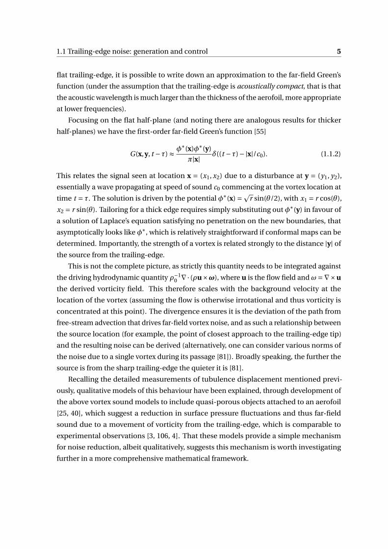
half-planes) we have the first-order far-field Green’s function [55]

G(x,y, t −τ) ≈ φ∗(x)φ∗(y)

π|x| δ((t −τ)−|x|/c0). (1.1.2)

This relates the signal seen at location x = (x1, x2) due to a disturbance at y = (y1, y2),

essentially a wave propagating at speed of sound c0 commencing at the vortex location at

time t = τ. The solution is driven by the potential φ∗(x) =pr sin(θ/2), with x1 = r cos(θ),

x2 = r sin(θ). Tailoring for a thick edge requires simply substituting out φ∗(y) in favour of

a solution of Laplace’s equation satisfying no penetration on the new boundaries, that

asymptotically looks like φ∗, which is relatively straightforward if conformal maps can be

determined. Importantly, the strength of a vortex is related strongly to the distance |y| of

the source from the trailing-edge.

This is not the complete picture, as strictly this quantity needs to be integrated against

the driving hydrodynamic quantity ρ−10 ∇· (ρu×ω), where u is the flow field and ω=∇×u

the derived vorticity field. This therefore scales with the background velocity at the

location of the vortex (assuming the flow is otherwise irrotational and thus vorticity is

concentrated at this point). The divergence ensures it is the deviation of the path from

free-stream advection that drives far-field vortex noise, and as such a relationship between

the source location (for example, the point of closest approach to the trailing-edge tip)

and the resulting noise can be derived (alternatively, one can consider various norms of

the noise due to a single vortex during its passage [81]). Broadly speaking, the further the

source is from the sharp trailing-edge the quieter it is [81].

Recalling the detailed measurements of tubulence displacement mentioned previ-

ously, qualitative models of this behaviour have been explained, through development of

the above vortex sound models to include quasi-porous objects attached to an aerofoil

[25, 40], which suggest a reduction in surface pressure fluctuations and thus far-field

sound due to a movement of vorticity from the trailing-edge, which is comparable to

experimental observations [3, 106, 4]. That these models provide a simple mechanism

for noise reduction, albeit qualitatively, suggests this mechanism is worth investigating

further in a more comprehensive mathematical framework.

6 Introduction

The vortex sound model framework is limited. Full use of the tools of conformal maps

requires limitation to two dimensions, as does useful implementation of any vortex shed-

ding at the trailing-edge (for example by releasing a vortex at each timestep [54] or using

the Brown and Michael formulation [23, 53]). This limits use in investigating the funda-

mentally three-dimensional behaviour of finlets. Further, vortex sound models typically

neglect underlying viscous considerations, important in thin regions near surfaces. Given

experimental measurements show not only a broad movement in location of turbulence

but also a stronger variation in boundary-layer shear, inclusion of some viscous effects, if

only in the imposition of background rotational flow, appears necessary.

1.1.4 Rapid Distortion Theory

Rapid distortion theory (RDT) has its roots in the study of the development of turbulence

by Batchelor and Proudman [13]. At the fundamental level, it concerns the distortion

of turbulence as it passes through a region of large-scale straining motions [60]. This

assumption of rapid convection allows linearisation of the governing vorticity equation

around some mean flow, consistent with Taylor’s hypothesis, that in a frame moving with

the mean flow the turbulence will be nearly frozen [108]. This hypothesis cannot hold if

nonlinear terms (for example Reynolds stresses) and viscous terms (leading to dissipation

of eddies) are important, though arises naturally from linearisation of the Euler equations

(in which viscosity is treated as negligible, at least with regards the perturbations). RDT

was applied in an aeroacoustic sense in 1978 by Goldstein [42], considering perturbations

to some background irrotational flow. This is broadly equivalent to the vortex sound

analysis above, in the limit that vortex self-propulsion (due to the flow generated by the

perturbation vorticity itself) can be neglected.

In the absence of background vorticity, perturbation entropy and vorticity are con-

vected with the mean flow [47]. The perturbation flow can be decomposed as u′ =∇φ+uR ,

where the rotational perturbation is solely within uR . In the absense of background rota-

tion, linearisation of the background flow results in decoupled equations for φ (satisfying

a convected wave equation) and for uR (convected with the mean flow), and we can thus

describe φ as the usual acoustic velocity potential. Only this latter term carries with it a

pressure perturbation: the vortical and entropic solutions are silent. We can, however,

define uR as the gust solution, generalising the vortical solution in the vortex sound model

above.

For sheared flow, the background flow is not irrotational. Such flows could arise due

to a jet or a non-negligible boundary-layer near an object. Fundamentally, this leads

to a coupling between vortical and acoustic components of the velocity perturbation.

1.1 Trailing-edge noise: generation and control 7

However, the idea of a gust can be generalised in the case of transversely sheared flow,

as identified by Goldstein et al. in the late 1970s [42, 44] and recently extended [46, 48].

In the case of a parallel background flow, it is possible to identify two quantities that are

convected with the background flow, which in turn drive the development of physical

variables. Most importantly, the pressure perturbation is driven by a single convected

quantity, which can be identified as a generalisation of the perturbation vorticity. The

details of this can be found in §2.

That perturbation vorticity is convected in sheared flow is the classical result of Orr

[80], from investigations into the stability of simply sheared Couette flow. If the back-

ground shear is constant, then perturbation vorticity is exactly convected, which in turn

drives the fluid motion through the solution of the Poisson equation. This setup, whilst

fundamentally concerned with incompressible (and as such non-acoustic) motions, can

be utilised in the compressible case as an inner problem, provided the boundary-layer

thickness is negligible on the lengthscale of acoustic fluctuations. This is typically true

provided frequencies are suitably low and the background flow is slow compared to the

speed of sound. Even for higher frequencies, the linear shear approximation removes

some of the underlying mathematical difficulties, based around the singularity of the

governing differential equation when the wavenumber of a disturbance corresponds to the

convective wavenumber due to the background flow. This linear shear approximation re-

moves this difficulty, though similar problems may arise in more complicated geometries

[22].

Even this simple setup, which in the incompressible limit permits analytical solutions,

can highlight interesting phenomena. While a mass source placed in uniform flow cannot

generate any vortical (rotational) perturbations, through the interaction with background

shear a trailing vortical sheet can be generated [92]. This recent result is extended in

this work by considering only a finite region of shear (considered previously by, for ex-

ample, Schuster [96]), which allows precise matching to an acoustic solution beyond the

boundary-layer, and by considering an more refined piecewise-linear approximation to

the background flow. This naturally requires discontinuity in background shear, which

generates atypical behaviour and shall be investigated in detail.

This model is useful in the context of noise control devices, particularly finlet-like

structures. These devices are small compared to the boundary-layer thickness, for example

Afshari et al. [4] considered devices with heights around 0.16δ, where δ is the boundary-

layer thickness. With regards the mean flow, this leads to a substantial increase in near-

wall shear. Similar models of fibre canopies have been considered [27], considering the

attenuation of instability waves by the localised shear layer around the fibres. With the

8 Introduction

mean flow profile an input to the model, it is straightforward to investigate these effects in

a RDT framework.

A second benefit of the model is control of the gust solution. As the previous vortex

models have shown, vorticity deflection can have a large impact on the scattered noise,

and this model gives a handle on vorticity deflection (through the convected quantity

generalising vorticity) within an explicit boundary-layer context. Given repeated measure-

ments of noise control devices show a general movement of eddies away from scattering

surfaces, it is worth quantifying the effect this might have on scattered noise in the far-field.

Indeed, for lower frequencies, with acoustic wavelengths much larger than boundary-layer

thicknesses, we expect minimal effect from the boundary-layer structure, which is on a

scale essentially unseen by the acoustic disturbance. However, regarding vorticity as the

source of noise, the location and strength of this hydrodynamic source itself, strongly

dependent on boundary-layer structure, is expected to have a great impact on percieved

noise, through the scattering process.

It is worth comparing the discussion here with Amiet’s formula above, (1.1.1). That

formulation is derived by considering the scattering of some harmonic “gust” of the form

exp(iω(t −x1/Uc )

), (1.1.3)

that is, a wave moving at some convection velocity Uc which is less than the free-stream

velocity, beyond the boundary-layer. The scattering of such a gust can be computed

exactly in terms of exponential integrals, using either Schwarzschild’s solution [97] (a

Green’s function for half-plane scattering) or more directly through application of the

Wiener-Hopf technique [79], discussed below. This gives rise to the transfer function L.

As well as being somewhat agnostic to the exact structure of the forcing term (since the

main experimental input is the wall pressure, again modified by the source structure), it

requires measurement or input of the convection velocity Uc . Conversely, with the RDT

formulation, the convection velocity is an intrinsic character of the vorticity distribution,

being the background velocity at the location of the vorticity.

1.1.5 Scattering

The solution to the classical Sommerfeld scattering problem, of an (electromagnetic) wave

scattered by a half-plane, dates back to 1896 [104], giving rise to the well-known diffraction

pattern from a sharp edge. Solutions can also be derived via Schwarzschild’s method [97],

which constructs a Green’s function for the half-plane problem (and so, given surface

forcing, can compute the far-field radiated noise). Both these solutions, however, are

1.1 Trailing-edge noise: generation and control 9

solely for Helmholtz equation (the time-harmonic wave equation), with reasonably simple

imposed boundary conditions.

The Wiener-Hopf technique was developed as a way of solving a class of singular

integral equations in 1931 [117]. It was noted by a variety of authors in the 1940s that

the method could be applied to (acoustic or electromagnetic) diffraction problems, and

we consider primarily the formulation constructed by Jones in 1950 [64], which works

directly in the Fourier transformed space rather than direct and consistent consideration of

integral equations, and is the approach taken by Noble in the classical reference book [79].

We essentially extend the range of problems that can be solved by the Fourier transform

(and other transforms) with discontinuous boundary data, by considering the complex

analyticity of the partial transform of the data. As well as providing an elegant analytic

solution to the simple diffraction problems (and more complicated, similar problems),

it is useful even for more complicated problems. In particular, the method offers a great

degree of control at discontinuities of boundary conditions. Numerical computation of

scattering problems is difficult near sharp corners, in particular the application of the

unsteady Kutta condition [31] (the insistence that perturbations are minimally singular at

the trailing-edge of an aerofoil), due to the presence of (singular) eigensolutions radiating

from the tip. Analytic application of the Kutta condition allows the correct eigensolution

to be chosen, which is vital for correct understanding of the far-field noise [8].

Much acoustic consideration of scattering problems using the Wiener-Hopf technique

focusing on leading- and trailing-edges, typically considering perturbations to uniform

flow, or to first-order (irrotational) corrections due to camber, angle of attack or aerofoil

thickness [75, 76, 9]. However, the method is applicable to sheared flow and to scattering

from discontinuities along a continuous boundary, for example at the start or end of

a lined section of wing. Consideration of background rotational flow typically leads to

governing equations that are not analytically tractable, except in certain limits, but the

complex analytic methods permitted by the Wiener-Hopf technique transfer over even

if numerical computation of functions is required. The junction scattering problem

(between a hard-wall and a soft-wall, and vice versa) has been considered previously [93,

101] in an analytically tractable limit, which does however pose difficulties in computation

of the scattered solution. By considering the numerical analogue of this problem, in the

suitable limit of speed of sound tending towards infinity, it is possible to reevaluate the

results suggested by this analytic analysis.

10 Introduction

1.1.6 Acoustic linings

This work will discuss the evolution of perturbations above a lined surface. Acoustic

linings, typically acoustic damping materials made up of an array of Helmholtz resonators,

are used throughout aircraft to reduce noise, most notably within the turbofan aeroengine

(the most important source of take-off noise), and could be considered a model of the

soft upper side of the wing of an owl [38]. A variety of complexity in liner models can be

considered, for example the nonlinear models of Innes and Crighton in 1989 [62] and

more recently of Singh and Rienstra [102]. A typical simple model of a linear posits a

relationship between the pressure and the velocity on a surface, linked by some complex

impedance Z which depends on the frequency ω of the disturbance. We consider a locally

reacting liner, which relates pressure and velocity perturbations at a surface via some

linear relationship p ′ = Z v ′, where v ′ is the wall-normal velocity perturbation [59], and

Z contains terms relating to the adsorbption and reactance of the liner. This should be

suitably modified in the presence of background flow and shear [61, 77] (see (2.4.4)).

Much study has been done of this problem in acoustic ducts (as opposed to distur-

bances above flat surfaces in this work). Typically, in a duct with a hard boundary, acoustic

disturbances can be characterised by a complete set of modal disturbances. These propa-

gate either upstream or downstream from some source, and are either cut-off (decaying

exponentially away from the source) or cut-on (neutrally stable propagating down the

duct). These can broadly be associated with the acoustic branch cut in the problem

considered here, which replaces a line of modal solutions with a branch cut in complex

wavenumber space. For a lined duct, these modes are all attenuated, but can still broadly

be associated as either upstream or downstream propagating, and as generalisations of

cut-on or cut-off [82].

Importantly, however, a new collection of modes appears in considering disturbances

to background flow above a lined wall. These surface modes remain confined to a very

thin region near the wall, and were identified by Rienstra [86, 87]. The number of such

modes differs based on the presence or not of background shear and of the exact flow

configurations, and they can be quite difficult to find [88]. For disturbances to uniform

flow, up to four such modes could be found, which rises to six when background shear is

included [111, 110]. The potential instability of such modes causes problems, as identified

by Rienstra and Darau [91] and by Brambley (and Peake) [18, 19], of the Myers boundary

condition being fundamentally ill-posed in the limit of the boundary-layer thickness

tending towards zero, and as such some finite region of inviscid boundary-layer must be

included in the analysis, motivating the work of Rienstra, Darau and Brambley [92] in

considering hydrodynamic disturbances to simple linear shear, which allows exact com-

1.2 Thesis structure 11

putation of the surface mode behaviour in sheared flow, and a corresponding numerical

analysis [22] considering critical-layer effects. The modal scattering problem has been

considered in ducts [85, 89]. Whilst surface modes are fundamentally hydrodynamic, and

do not themselves generated far-field noise, the scattering of excited surface modes, for

example at the trailing-edge of a section of lining could be a source. Inclusion of realistic

shear within a boundary-layer further allows another look at scattering from a lined wall,

considered previously in a limited case by Rienstra and Singh [93, 101].

1.2 Thesis structure

This work gradually builds up a picture of the gust solution in transversely sheared flow,

before computing the scattering of such a solution firstly from the junction between two

liners before focusing on the trailing-edge scattering problem. The goal of this thesis is

to understand the fundamental mechanisms behind control of the boundary-layer in

reduction of far-field noise, be it from point disturbance or scattering from boundary

discontinuities.

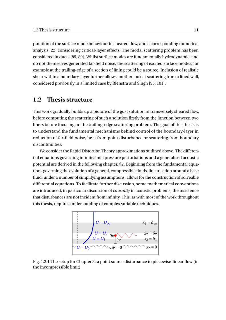
We consider the Rapid Distortion Theory approximations outlined above. The differen-

tial equations governing infinitesimal pressure perturbations and a generalised acoustic

potential are derived in the following chapter, §2. Beginning from the fundamental equa-

tions governing the evolution of a general, compressible fluids, linearisation around a base

fluid, under a number of simplifying assumptions, allows for the construction of solveable

differential equations. To facilitate further discussion, some mathematical conventions

are introduced, in particular discussion of causality in acoustic problems, the insistence

that disturbances are not incident from infinity. This, as with most of the work throughout

this thesis, requires understanding of complex variable techniques.

x2 = δ∞

x2 = δ2

x2 = δ1

x2 = 0U =U0

U =U1

U =U2

U =U∞

q0y2

Lψ= 0

Fig. 1.2.1 The setup for Chapter 3: a point source disturbance to piecewise-linear flow (inthe incompressible limit)

12 Introduction

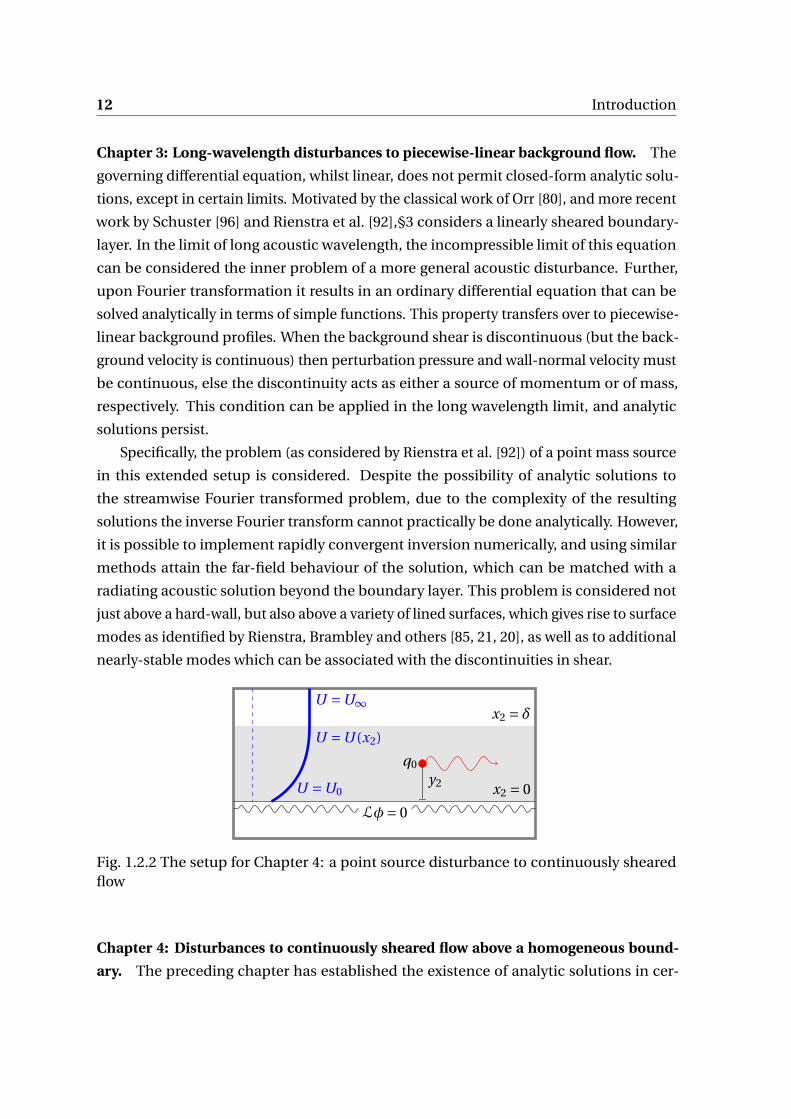
Chapter 3: Long-wavelength disturbances to piecewise-linear background flow. The

governing differential equation, whilst linear, does not permit closed-form analytic solu-

tions, except in certain limits. Motivated by the classical work of Orr [80], and more recent

work by Schuster [96] and Rienstra et al. [92],§3 considers a linearly sheared boundary-

layer. In the limit of long acoustic wavelength, the incompressible limit of this equation

can be considered the inner problem of a more general acoustic disturbance. Further,

upon Fourier transformation it results in an ordinary differential equation that can be

solved analytically in terms of simple functions. This property transfers over to piecewise-

linear background profiles. When the background shear is discontinuous (but the back-

ground velocity is continuous) then perturbation pressure and wall-normal velocity must

be continuous, else the discontinuity acts as either a source of momentum or of mass,

respectively. This condition can be applied in the long wavelength limit, and analytic

solutions persist.

Specifically, the problem (as considered by Rienstra et al. [92]) of a point mass source

in this extended setup is considered. Despite the possibility of analytic solutions to

the streamwise Fourier transformed problem, due to the complexity of the resulting

solutions the inverse Fourier transform cannot practically be done analytically. However,

it is possible to implement rapidly convergent inversion numerically, and using similar

methods attain the far-field behaviour of the solution, which can be matched with a

radiating acoustic solution beyond the boundary layer. This problem is considered not

just above a hard-wall, but also above a variety of lined surfaces, which gives rise to surface

modes as identified by Rienstra, Brambley and others [85, 21, 20], as well as to additional

nearly-stable modes which can be associated with the discontinuities in shear.

x2 = δ

x2 = 0U =U0

U =U (x2)

U =U∞

q0

y2

Lφ= 0

Fig. 1.2.2 The setup for Chapter 4: a point source disturbance to continuously shearedflow

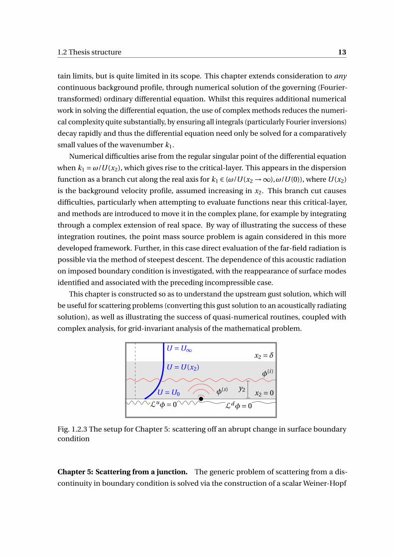
Chapter 4: Disturbances to continuously sheared flow above a homogeneous bound-

ary. The preceding chapter has established the existence of analytic solutions in cer-

1.2 Thesis structure 13

tain limits, but is quite limited in its scope. This chapter extends consideration to any

continuous background profile, through numerical solution of the governing (Fourier-

transformed) ordinary differential equation. Whilst this requires additional numerical

work in solving the differential equation, the use of complex methods reduces the numeri-

cal complexity quite substantially, by ensuring all integrals (particularly Fourier inversions)

decay rapidly and thus the differential equation need only be solved for a comparatively

small values of the wavenumber k1.

Numerical difficulties arise from the regular singular point of the differential equation

when k1 =ω/U (x2), which gives rise to the critical-layer. This appears in the dispersion

function as a branch cut along the real axis for k1 ∈ (ω/U (x2 →∞),ω/U (0)), where U (x2)

is the background velocity profile, assumed increasing in x2. This branch cut causes

difficulties, particularly when attempting to evaluate functions near this critical-layer,

and methods are introduced to move it in the complex plane, for example by integrating

through a complex extension of real space. By way of illustrating the success of these

integration routines, the point mass source problem is again considered in this more

developed framework. Further, in this case direct evaluation of the far-field radiation is

possible via the method of steepest descent. The dependence of this acoustic radiation

on imposed boundary condition is investigated, with the reappearance of surface modes

identified and associated with the preceding incompressible case.

This chapter is constructed so as to understand the upstream gust solution, which will

be useful for scattering problems (converting this gust solution to an acoustically radiating

solution), as well as illustrating the success of quasi-numerical routines, coupled with

complex analysis, for grid-invariant analysis of the mathematical problem.

x2 = δ

x2 = 0U =U0

U =U (x2)

U =U∞

φ(i )

y2φ(s)

Luφ= 0 Ldφ= 0

Fig. 1.2.3 The setup for Chapter 5: scattering off an abrupt change in surface boundarycondition

Chapter 5: Scattering from a junction. The generic problem of scattering from a dis-

continuity in boundary condition is solved via the construction of a scalar Weiner-Hopf

14 Introduction

equation. This is solved via appeal to known complex analyticity of transformed boundary

conditions, coupled with some knowledge of the behaviour of the scattered solution near

the junction itself, typically by minimising any singularities at this point. This complex

analytic technique gives solutions that are accurately known, at least in terms of integrals,

and can readily be computed numerically.

By considering the scattering of perturbations to a realistically sheared boundary layer

as it passes over the leading- or trailing-junction of a lined surface, it is possible to quantify

the far-field noise due to this scattering alone. This is extended to considering scattering

by a section of lining of finite length. If surface modes are excited at the first junction, the

scattering and restabilisation of these modes at the end of the lining can be a very strong

source of sound, even without direct acoustic coupling between the two junctions.

Previous work [101] has considered the hard-soft and soft-hard junction scattering

problem in the incompressible limit, with a constant shear, infinite thickness boundary-

layer, which was then matched to an outer solution. This problem is reanalysed here,

considering the incompressible case as instead the limit at the speed of sound, c0 →∞,

in the compressible framework. This numerical approach allows precise evaluation of

the strengths of the previous work, highlighting difficulties due to the loss of a strip of

analyticity in the incompressible limit, and the resulting difficulties this poses for the

Wiener-Hopf technique. Inclusion of a shear layer further allows precise evaluation of

scattering when the background profile is forced to be non-slipping, which has previously

created issues [20].

x2 = δ+

x2 = 0

x2 = δ−

U =U0

U =U+(x2)

U =U+∞

U =U0

U =U−(x2)

U =U−∞

φ(i )

φ(s)LZφ= 0

Fig. 1.2.4 The setup for Chapter 6: a convected vortical disturbance scattering off a (poten-tially lined) sharp trailing-edge

1.3 Summary of aims and objectives 15

Chapter 6: Trailing-edge scattering. The final substantial chapter focuses on the prob-

lem of scattering from a trailing-edge, which can be linked to the problems considered in

§5 if the background flow profile is symmetric, though this model allows relaxation of this

assumption. Further, it is reasonably straightforward to permit consideration of scattering

from a lined trailing-edge, which is also done, and may generated upstream-propagating

surface modes as well as modes propagating in the wake. Again, far-field evaluation allows

rapid determination of the dominant acoustic contribution through the steepest descent

method. The basic layout of this chapter is shown in figure 1.2.4.

The previous chapter considered a convected vortex sheet, which bore similarities to a

perturbation vortex sheet. This term is carefully understood, and more general convected

generalised vortical disturbances within the boundary-layer are considered, in particular

how they scatter off the trailing-edge. The linearity of this model makes this a straight-

forward extension of the previous work, in particular the scattering problem extends

straightforwardly to more complicated incident disturbances. With the vortex sheet more

carefully understood, it is possible to directly analyse the effect on the amplitude of the

sound, as well as directivity, of variations in background shear and the upstream location

of the perturbation vortex sheet. We are therefore in a position to directly analyse the

noise control devices mentioned previously, particularly focusing on the experimental

measurements of background mean flow and of turbulence intensity within the boundary-

layer. This provides compelling evidence of the importance of turbulence location on

wall-pressure and, in turn, on far-field noise.

1.3 Summary of aims and objectives

This overall aim of this work is to explain the noise reduction mechanism of proposed

passive and active trailing-edge noise devices, through analysis of their observed effect on

boundary-layer shear and turbulence. These objectives are met through the analysis of

simplified mathematical models, attempting to include only the relevant physics, namely

the inclusion of shear in the background flow (typically focusing on a hydrodynamic

boundary-layer). Within the framework of this model the relevant trailing-edge scattering

problem is discussed, as well as extensions to other related problems. This in turn allows

additional study of scattering problems between lined surfaces and from a lined trailing-

edge.

Chapter 2

Mathematical formulation of Rapid

Distortion Theory

Consideration of linearised perturbations to transversely sheared background flow are

common to all the problems considered in this work, based on the earlier work of Gold-

stein and others [42, 44, 46]. The derivation of the fundamental equations governing

these perturbations are discussed here, along with some mathematical conventions and

techniques used throughout this work.

2.1 Basic concepts

2.1.1 Equations of fluid dynamics

In the continuum approximation, a fluid is characterised by its flow field u(x, t) and a

variety of other physical quantites, for example the pressure p(x, t) and density ρ(x, t),

which are functions of spatial position x and time t . A general fluid obeys the equations of

conservation of mass and momentum, which in differential form can be written

Dρ

Dt=−ρ∇·u, (2.1.1a)

Du

Dt=−∇p + f+∇·σ, (2.1.1b)

where we have introduced the material derivative

D

Dt= ∂

∂t+u ·∇, (2.1.2)

18 Mathematical formulation of Rapid Distortion Theory

which governs the rate of change of a quantity moving with the fluid. In (2.1.1b), f is some

body force acting on the fluid (for example gravity), and σ is the deviatoric stress tensor,

representing frictional forces between fluid elements.

For a Newtonian fluid, which includes air and water to a reasonable approximation,

the deviatoric stress tensor can be directly related to the rate of strain tensor ei j = ∂ui /∂x j ,

with σ = µ(e+eT ), where the proportionality constant µ defines the dynamic viscosity,

and in this case ∇·σ is simply µ∇2u.

Consider a fluid with a reference density ρ (for example, the density of the fluid when

stationary or moving at a constant velocity). Suppose this fluid is moving at a speed U

over some lengthscale L. We can then define the dimensionless Reynolds number, Re, as

Re = ρU L

µ(2.1.3)

which governs the balance between inertia and viscosity [12, 41]. For fluids with high Re

this suggests we can ignore the viscous terms. However, this is not a valid assumption near

the boundaries of the domain, which can be noted either by spotting that the reference

lengthscale, L, becomes small, or that the second derivative ∇2u could become very large

here. For the bulk fluid, away from the boundaries, it seems reasonably to broadly ignore

viscosity, though at times it may be reintroduced as appropriate. To quantify the Reynolds

number of interest, consider the flight of an owl. Large owls typically have a wing chord-

length of up to 400 mm (see for example Table 1 in [63], collated from other works). The

mean flight speed of a barn owl is of the order 5 ms−1[78, 38, 37]), which, with kinematic

viscosity of air, ν= µ/ρ, of the order ν≈ 1×10−5 m2s−1 gives a Reynolds number of the

order 1×105. Of course, if much finer lengthscales are looked at, for example the spacing

of fibres on the surface of the wing, much smaller Reynolds numbers are attained.

The equations governing motion of a compressible fluid are not closed, unlike their

incompressible counterparts, with another equation required to link pressure and density.

Under the assumption that acoustics are a adiabatic thermodynamic process not involving

any exchange of heat or dissipation, it is possible to write an energy equation in terms of

the entropy s. Any thermodynamic variable can be written in terms of the other two, and

so it follows that for a perfect gas

ds = cVdp

p− cp

dρ

ρ, (2.1.4)

2.1 Basic concepts 19

where cV and cp are the specific heats for constant volume and pressure respectively. In

the case that entropy is everywhere constant, so that ds = 0, this can be rewritten as

p

ργ= const. (2.1.5)

In this equation γ is the ratio of specific heat capacities, γ= cp /cV . This is the homentropic

assumption, and is slightly stronger than what is needed. We consider the more general

specification of an isentropic fluid: the entropy of a moving fluid element does not change,

and as suchDs

Dt= 0. (2.1.6)

Use of the differential form for ds immediately gives a relationship between the material

derivatives of p and ρ, as [41]Dp

Dt= γp

ρ

Dρ

Dt, (2.1.7)

where γp/ρ = (∂p/∂ρ

)s in the isentropic case. This corresponds to the (square of) the

usual definition of the speed of sound, as

c2 = ∂p

∂ρ

∣∣∣∣∣s

, (2.1.8)

with subscript s denoting the derivative at fixed entropy.

That the quantity c is indeed the speed of acoustic waves is most easily seen by con-

sidering small perturbations to quiescent flow of constant density ρ0 (and thus speed

of sound c0), neglecting quantities quadratic in perturbation variables and any external

forces. The governing equations reduce to

∂ρ′

∂t=−ρ0∇·u′, (2.1.9)

ρ0∂u′

∂t=−∇p ′, (2.1.10)

∂p

∂t= c2

0∂ρ

∂t. (2.1.11)

Elimination of density perturbations through use of the third equation into the first gives

∂p ′

∂t=−ρ0c2

0∇·u′. (2.1.12)

Taking the time derivative of this equation and the divergence of the equation for velocity

perturbations allows elimination of the cross term, ρ0∂/∂t (∇·u′), common to both equa-

20 Mathematical formulation of Rapid Distortion Theory

tions and results in a single second-order differential equation for pressure perturbations:

∂2p ′

∂t 2− c2

0∇2p ′ = 0. (2.1.13)

This is clearly a wave equation, with the wavespeed given, as expected, by the speed of

sound c0. This derivation, for a more complicated base flow, is revisited in the next section.

The above derivation supposed the speed of sound and the background density were

constant. This is broadly true if the Mach number is low, where we define the Mach

number Ma as

Ma = U

c0, (2.1.14)

for some reference speed of the fluid U and speed of sound c0. This assumption of constant

background density can be quantified somewhat, for example if we have a homentropic

flow with averaged flow speed upstream U∞ (with corresponding density ρ∞), then the

relationship with the local density ρ0 can be written [41]

(ρ0

ρ∞

)γ−1

= 1+ (γ−1)

c2∞(U 2

∞−U 2), (2.1.15)

and a low Mach number assumption allows the second term to be neglected. If we do

not make this assumption there may be some variation in background density ρ0 and

thus background speed of sound c0, and we keep this option in mind in later derivations,

though where Ma2 ≪ 1 we can reasonably take ρ0 and c0 constant in space.

2.1.2 Mathematical conventions

A few mathematical conventions will be used in this and following chapters, mostly to

simplify notation. This section gives a brief overview of the important points, most notably

the sign convention used for Fourier transformation.

Fourier transforms. Fourier transforms, both spatial and temporal, are used throughout

this chapter and the following. Where it is unambiguous, subscripts are used to define the

transform variable. For example, given a function f (x, t ) we have

f0(x,ω) =∫ ∞

−∞f (x, t )e−iωt dt (2.1.16)

2.1 Basic concepts 21

(or, if necessary,∫ T−T dt as T →∞) and

f1(k1,xT , t ) =∫ ∞

−∞f (x, t )e+i k1x1 dx1. (2.1.17)

with xT being the components of x other than x1. We define wall-normal and spanwise

Fourier transforms analogously to the streamwise case, with complex wavenumbers k2

and k3 respectively, denoted by subscript ·2 and ·3.

The inversion of these is given by

f (x, t ) = 1

2π

∫ ∞

−∞f0(x,ω)e iωt dω (2.1.18)

f (x, t ) = 1

2π

∫ ∞

−∞f1(k1, x2, t )e−i k1x1 dk1 (2.1.19)

These transformations stack to form multivariate transformations, if required. They can

also be applied to differential operators, normally through the transformations ∂/∂t 7→ iω

and ∂/∂x j 7→ −i k j .

Causality: Briggs-Bers and the radiation condition. Suppose we are considering the

problem of a point source near a boundary, with the domain extending to infinity both

upstream and downstream in the x1 direction (an open shear flow) and to x2 →∞. If the

source is switched on at a given time, for example t = 0 without loss of generality, then it is

reasonable to insist that there is no disturbance before the source is switched on. Further,

we insist that, spatially, no waves propagate inwards from infinity: all disturbances are

created at the source. Whilst these conditions are easy to understand physically, care must

be taken to implement them in Fourier space.

We first deal with the temporal causality condition, that there is no disturbance before

the source is turned on. Consider, for a generic linear partial differential operator D in one

spatial dimension, the equation governing some disturbance φ with some source S(t , x1):

D

(∂

∂t,∂

∂x1

)φ(t , x1) = S(t , x1) (2.1.20)

with S ≡ 0 for t < 0. We impose the same condition on φ, that φ≡ 0 for t < 0. We apply the

double Fourier transform as outlined above, with

φ01(ω,k1) =∫ ∞

−∞

∫ ∞

−∞φ(t , x1)exp

(−i (ωt −k1x1))

dt dx1 (2.1.21)

22 Mathematical formulation of Rapid Distortion Theory

which simply reduces (2.1.20) to

D01(ω,k1)φ01(ω,k1) = S01(ω,k1), (2.1.22)

an algebraic equation. The dispersion function D01 is obtained simply by substituting

∂/∂t = iω and ∂/∂x1 = −i k1 into the expression for D. This is trivial to solve in Fourier

space, as

φ01 = S01

D01(2.1.23)

We now invert the temporal Fourier transform. Inverting along the real axis, as per

(2.1.19), might give contributions for t < 0, which conflicts with the temporal causal-

ity assumption. We can choose the inversion contour, denoted Lω, to lie beneath all

singularities of S01/D01, with

φ1(t ,k1) = 1

2π

∫Lω

S01(ω,k1)

D01(ω,k1)exp(iωt )dω (2.1.24)

If Lω lies beneath all roots of the dispersion relation, D01 = 0 then we can close the

integration contour Lω, for t < 0, in the lower-half ω plane (LHωP). Since the integrand is

free of singularities, this is identically zero. The contribution from the closure contour in

the lower half plane decays, as the real part of iωt is negative. This is precisely analogous

to inversion of the Laplace transform, where the inverse contour is taken to the right of all

singularities in the s-plane: essentially the Laplace transformation and the causal Fourier

transformation equivalent with s 7→ iω.

Depending on what we want to do, there are two things we can now do. The majority

of the discussion in this work focuses on a harmonic disturbance. That is, the solution

oscillates in time at a single, real, frequency ω. This is slightly at odds with the above,

where a complete temporal solution was considered. In particular, a harmonic solution

proportional to exp(iωt) is non-causal, however we do want to use temporal causality

arguments. We can do this by taking the imaginary part of ω to be sufficiently large and

negative, and then relax it back to the real axis. This is analogous to continuing the process

that returned φ1 above, and carefully considering the spatial inversion contour, which

shall be done by way of illustration.

Suppose that there is a single temporal mode for which D01(ω,k1) = 0, given by ω(k1).

Since Lω lies beneath this singularity by construction, we can close in the upper half-plane

2.1 Basic concepts 23

and apply the residue theorem to give, for positive time,

φ1(t ,k1) =− i S01(ω(k1),k1)∂D01

∂ω(ω(k1),k1)

exp(−iω(k1)t ) (2.1.25)

Unlike the temporal inversion contour, there is no need for the spatial inversion con-

tour Fk1 to be anything other than the real axis: indeed, this is assumed for the existence

of spatial Fourier transforms (namely, decays as |x| →∞), as opposed to the causal as-

sumptions on the temporal transform. Thus, the precise solution φ can be obtained by

computing the standard spatial inversion of the above, noting that the singularities, in

the k1 plane, of the integrand of (2.1.24) will not cross Fk1 as ω varies: solutions k1(ω)

satisfying D01(ω,k1(ω)) are confined to loci in the upper- or lower-half k1 plane as ω

varies.

This observation allows relaxation of the Lω contour to the real axis, provided the Fk1

contour is suitably deformed so as to maintain the observation above. This is not always

possible, for example if two poles, on either side of the Fk1 contour for large negative Im(ω),

come together for some Im(ω) which is still non-zero, thereby forcing the Fk1 contour

between this pair of “pinched” contours. This leads to absolute instability, and is beyond

the scope of this work.

For the purposes of this work, we care only about identifying solutions which prop-

agate upstream and those that propagate downstream, analogously to the above. For

negative imaginary part of ω, it is possible to unambiguously identify poles of Fourier

transformed quantities with either the upper- or lower-half k1 plane, corresponding re-

spectively to upstream and downstream-propagating modes upon inversion. This requires

further that no branch cuts cross the real k1 axis, which for example determines the di-

rection of the branch cuts of γ=√

k21 −ω2/c2

0 (or similar) later (see (4.2.12)), with branch

points connected each other through complex infinity. The Briggs-Bers procedure, as we

understand it, then requires that these modal solutions, and any branch cut contributions,

remain in the same generalised "half-plane", with the complex plane bisected by F (k1),

as the imaginary part of ω is relaxed to zero. This can lead to unstable modal solutions

growing downstream, for example, for real ω. This is demonstrated for pressure-release

modes in §3.6. Essentially the condition that quantities are integrable (and thus we can

compute Fourier transforms) is replaced by a condition that nothing propagates inwards

from upstream or downstream infinity, even if it means the outward-radiating solution is

infinite there (and thus doesn’t have a classical Fourier transform). This is demonstrated

schematically in figure 2.1.1.

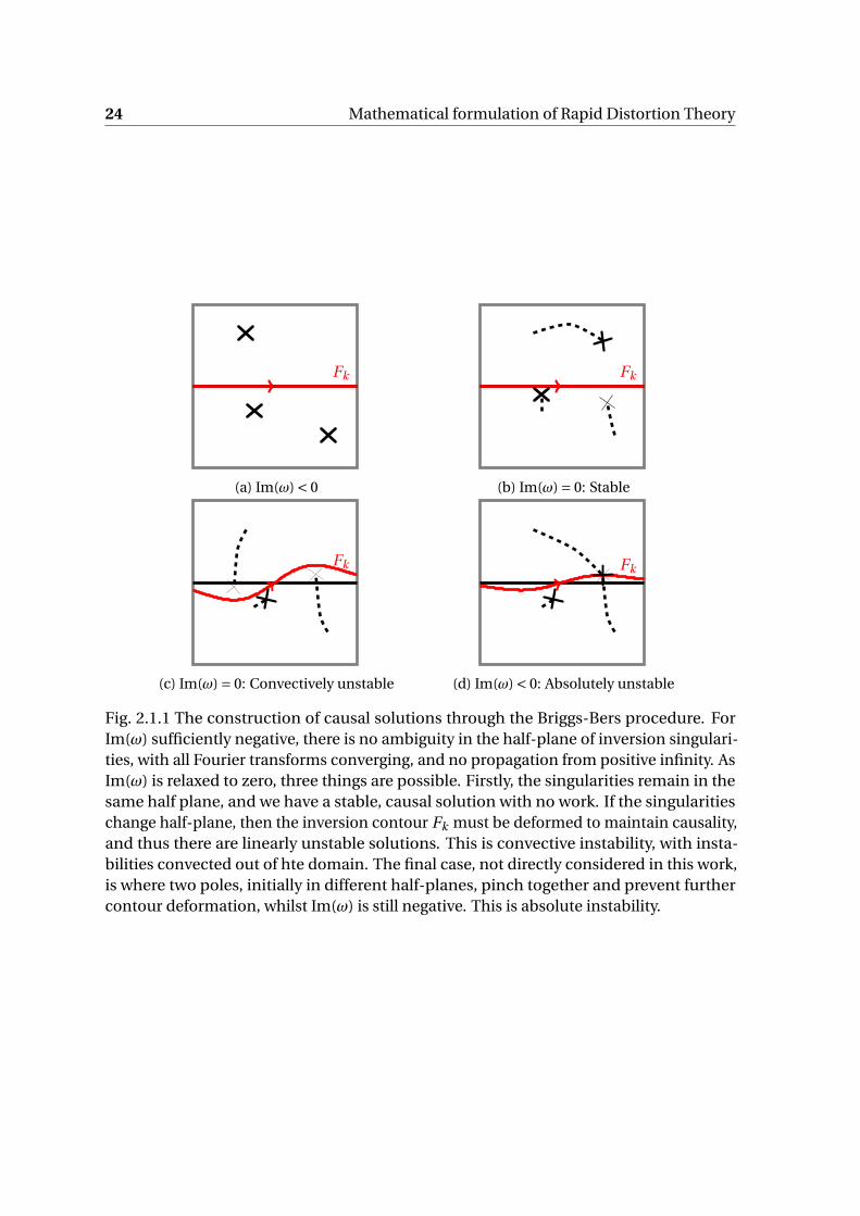
24 Mathematical formulation of Rapid Distortion Theory

Fk

(a) Im(ω) < 0

Fk

(b) Im(ω) = 0: Stable

Fk

(c) Im(ω) = 0: Convectively unstable

Fk

(d) Im(ω) < 0: Absolutely unstable

Fig. 2.1.1 The construction of causal solutions through the Briggs-Bers procedure. ForIm(ω) sufficiently negative, there is no ambiguity in the half-plane of inversion singulari-ties, with all Fourier transforms converging, and no propagation from positive infinity. AsIm(ω) is relaxed to zero, three things are possible. Firstly, the singularities remain in thesame half plane, and we have a stable, causal solution with no work. If the singularitieschange half-plane, then the inversion contour Fk must be deformed to maintain causality,and thus there are linearly unstable solutions. This is convective instability, with insta-bilities convected out of hte domain. The final case, not directly considered in this work,is where two poles, initially in different half-planes, pinch together and prevent furthercontour deformation, whilst Im(ω) is still negative. This is absolute instability.

2.2 A wave equation for pressure 25

The above primarily concerns itself with the streamwise direction, that nothing is inci-

dent from x1 →±∞. We must add a further radiation condition that waves are outgoing

at infinity in all directions. For harmonic waves, with timelike dependence e iωt , this is

simply the condition that solutions have wavelike dependence

p ′ ∼ exp(i (ωt −k ·x)) (2.1.26)

as x →∞, which can be written more precisely, for an n-dimensional solution to Helmholtz

equation, as

lim|x|→∞

xn−12(∇+ i k0

)p ′ = 0 (2.1.27)

with k0 =ω/c0 the Helmholtz number [105]. This is a condition of no energy coming from

infinity. It is important to check this condition is satisfied, with careful choice of sign

depending on the choice of Fourier transformation conventions. Typically, for the work in

this and later chapters, we utilise the condition that streamwise transformed, harmonic

solutions look like e−γx2 as x2 →∞, where γ has positive real part.

Plotting complex functions. Functions of a complex variable, w = f (z) = f (x + i y), are

ubiquitous throughout this work. There are a variety of methods of visualising complex

analytic functions. Whilst sometimes the real and imaginary parts of a map will be plotted

separately, which is sometimes useful (for example in determining contours on which

the imaginary part of a function is constant), typically the most useful plot is a plot of

the complex phase [113, 103], where the hue of the plot is associated with the complex

argument. This can be generalised to associate, for example, the brightness of the plot

with the magnitude of the complex function. Since both hue and argument are periodic,

such plots clearly show up singularities and branch cuts in the complex plane, and will be

used throughout this work without comment. An example of this plot showing branch

cuts can be seen later in figure 4.2.1, for the acoustic exponent γ(k1), which has two finite

branch points (joined through infinity).

2.2 A wave equation for pressure

The introduction saw a quick derivation of the wave equation for small, acoustic pres-

sure perturbations to a quiescent flow. This derivation is now extended to linearised

perturbations to a prescribed parallel flow, resulting in a more complicated equation

governing pressure fluctuations. In particular, we focus on a boundary-layer flow, where

there is a uniform flow sufficiently far away from the boundary along x2 = 0 (x2 being

26 Mathematical formulation of Rapid Distortion Theory

the wall-normal coordinate), in the streamwise (x1) direction. Within the boundary-layer

itself, for 0 < x2 < δ, the background flow may be sheared.

This can be generalised to a wake or a jet, where there is a finite region, δ− < x2 < δ+,

for which the background shear U ′(x2) is non-zero, with the background flow otherwise

being constant beyond this region. The derivation of the equations assumes nothing

more than the background flow is sheared, so it is applicable to sheared flow in a duct, for

example, once further geometrical factors are included, which gives rise to the Pridmore-

Brown equations [82]. Application of this Rapid Distortion Theory argument (the basis for

neglection of nonlinear terms and effects of viscosity: convection drives perturbations

through the domain on a much more rapid timescale than that of the effect of viscosity and

nonlinearity) to boundary-layer and jet flow has been considered in detail by Goldstein

and others [42, 44, 46, 48], and it is this work that forms the basis of this derivation.

2.2.1 Assumptions

As suggested above, we make a variety of initial assumptions. The Reynolds number is

assumed large, allowing viscosity to be neglected in the momentum equation. While

this assumption cannot be true near boundaries (where the length scales of interest are

small), we assume that we are always far enough away from surfaces that viscous effects

on perturbation quantities can be neglected 1. We make the further assumption that

any flow we are considering is isentropic, allowing closure of the system of governing

equations written in the following form

Dρ

Dt+ρ∇·u = 0, (2.2.1a)

ρDu

Dt+∇p = 0, (2.2.1b)

Ds

Dt= 0. (2.2.1c)

If we consider the entropy as a function of density and pressure, s = s(ρ, p) then the

energy equation (2.2.1c) can be rewritten, linking pressure and density via the speed of

soundDp

Dt= c2 Dp

Dt. (2.2.2)

1This assumption must be relaxed when scattering problems are considered, with the unsteady Kuttacondition taking into account the effect of viscosity near sharp junctions, as seen in later chapters.

2.2 A wave equation for pressure 27

This in turn allows combination of the mass (2.2.1a) and energy equations (2.2.1c) into a

single equationDp

Dt+ c2ρ∇·u = 0. (2.2.3)

As above, making the slightly stronger assumption that the fluid we’re considering

is an ideal gas, for example air, then pressure and density can be related to the speed of

sound via

c2 = γp

ρ, (2.2.4)

where γ is the adiabatic index (for air, around 1.4 [116] ). This allows replacement of c2ρ

by γp if appropriate.

We now consider small, compressible disturbances to some prescribed, steady back-

ground flow. We assume that this background flow, u0, is rectilinear and does not develop

as it moves downstream, and as such is independent of the coordinate x1 which we de-

fine as the streamwise coordinate. The remaining spatial coordinates shall be called the

transverse coordinates, xT = (x2, x3). Typically we shall consider x2 to be a wall-normal

coordinate and x3 a spanwise coordinate, with respect to a horizontal aerofoil, though

for the present the general case is considered. With these assumptions the base flow

u0 = U (xT )e1 for some scalar U . For this and later chapters, we assume U is constant

outside some boundary-layer (x2 > δ+ > 0, x2 < δ− < 0), though this does not effect the

derivation of the governing equations.

2.2.2 Compressible Rayleigh’s equation

Denoting perturbation quantities with a prime, the total velocity is written as u(x, t) =u0(xT )+u′(x, t ). Similarly, the total pressure is decomposed as p(x, t ) = p0(xT )+p ′(x, t ) and

density ρ(x, t) = ρ0(xT )+ρ′(x, t), with mean quantities ·0 depending only on transverse

position xT and, like u0, assumed known. The stronger assumption of parallel, transversely

sheared background flow indicates, from (2.2.1b), that the background pressure p0 is

temporally and spatially constant. We also define the convective derivative with respect

to the base flowD0

Dt= ∂

∂t+u0 ·∇ = ∂

∂t+U

∂

∂x1

. (2.2.5)

28 Mathematical formulation of Rapid Distortion Theory

The governing equations, linearised around the parallel base flow u0 =U (xT )e1 (i.e.

neglecting quantites quadratic or smaller in primed quantities) are

D0p ′

Dt+ c2

0ρ0∇·u′ = 0, (2.2.6a)

ρ0D0u′

Dt+ρ0u′

T ·∇T U e1 +∇p ′ = 0, (2.2.6b)

with u′T = (0,u′

2,u′3) (so that u′ = u′

1e1 + u′T ) and ∇T = (0,∂/∂x2,∂/∂x3) the transverse

components of the perturbation velocity field and gradient operator respectively. The first

equation requires the assumption that we have an ideal gas, and so c20ρ0 can be regarded

as constant. Combining these linearised governing equations through

D0

Dt

[D0

Dt(2.2.6a)−∇· (c2

0(2.2.6b))

]+2c2

0∂

∂x1

(2.2.6b) ·e1 (2.2.7)

gives (the compressible) Rayleigh’s equationD0

Dt

[D2

0

Dt 2−∇· (c2

0∇)

]+2c2

0∂U

∂x j

∂2

∂x1∂x j

p ′ = 0. (2.2.8)

This reduces to (a convected derivative of) the usual (convected) wave equation in regions

with constant background flow, with the shear-dependent term ∂U /∂x j vanishing.

Depending on the context, this might also be referred to as the Pridmore-Brown equa-

tion [82], which is typically used for this equation in a cylindrical duct (and often after

Fourier expansion in the azimuthal direction, and Fourier transformation in the stream-

wise direction, i.e. the resulting r -dependent ODE). This does not change the equation

above, but it differs from the Cartesian case primarily through the introduction of factors

of 1/r in derivatives. In other contexts, particularly in the extension of Lighthill’s acoustic

analogy (thereby an exact rearrangement of the Euler equations, and with source terms

on the right-hand side), this is referred to as Lilley’s equation [45]. With the operator

referred to in the literature as both the Pridmore-Brown and Rayleigh operators, for preci-

sion we term the operator in Cartesian geometry as the compressible Rayleigh operator

throughout this work.

Inclusion of mass and momentum sources. With this setup, it is straightfoward to in-

clude mass and momentum sources by including non-zero terms on the right-hand side

of the governing equations of motion. With mass and momentum sources added to the

2.2 A wave equation for pressure 29

right-hand side of (2.2.1), we have

Dρ

Dt+ρ∇·u = q(x, t ), (2.2.9a)

ρDu

Dt+∇p = f(x, t ), (2.2.9b)

Ds

Dt= 0, (2.2.9c)

where q and f are mass and momentum (force) sources respectively, per unit volume. We

suppose these sources are the same order of magnitude as infinitesimal perturbations,

which would allow them to be added instead to the right-hand side of the linearised

equations, (2.2.6). By combining the governing equations, analogously to (2.2.7), we

obtain Rayleigh’s equation with source terms:D0

Dt

[D2

0

Dt 2−∇· (c2

0∇)

]+2c2

0∂U

∂x j

∂2

∂x1∂x j

p ′ = D0

Dt

[D0

Dt(c2

0 q)−∇· (c20f)

]+2c2

0∂ f1

∂x1

.

(2.2.10)

The spatial and temporal form of these sources can be chosen to match the problem, as

required.

Conditions at discontinuities of U and its derivatives. We need not assume U or its

derivatives are continuous, though relaxing this assumption requires care on conditions

applied to perturbation quantities at these points. The underlying physical assumptions

are of continuity of particle displacement and no net force acting across such a junction

(an assumption that also holds across a wake). We suppose there is such a discontinuity at

x2 =χ2 and define the jump across χ2 for some function f as

[f]χ2

= f (χ+2 )− f (χ−2 ), (2.2.11)

with the limit f (χ±2 ) defined as limx2→χ2 f (x2) from x2 ≷χ2 respectively. With this notation,

we have

[p ′]

χ2= 0, (2.2.12)

v ′(χ±2 ) = D±0 η

Dt(x1, x3, t ) (2.2.13)

with D±0 /Dt the mean-flow material derivative for x2 ≷χ2, and particle displacement η

continuous across χ2. It is straightforward to eliminate η if it is, for example, harmonic

30 Mathematical formulation of Rapid Distortion Theory

in its variables. In the special case of continuous U (but discontinuous ∂U /∂x2) then we

simply have [v ′]

χ2= 0 (2.2.14)

In later chapters, we assume the background flow U is everywhere continuous, even if the

derivative is not. We therefore need only impose conditions of continuity of v ′ and p ′ at

discontinuities of ∂U /∂x2.

2.3 The adjoint problem for general continuous background

profile

Typically for acoustic problems it might be possible to construct an acoustic potential, φ,

from which it is possible to derive representations of pressure and velocity fluctuations.

In the simplest case of perturbations to a quiescent fluid, these are given simply by

u′ =∇φ, p ′ =−ρ0∂φ

∂t, (2.3.1)

with the acoustic potential satisfying the usual wave equation. This naturally extends to

uniform background flow by replacement of time derivatives with convective derivatives,

and we can derive a partial differential equation for φ from which all physical variables

can be extracted.

Following Goldstein [44], this can be generalised to include shear. For reasons that

become clear in the derivation, we suggest a generalised acoustic velocity potentialφ such

that

p ′ =−D30φ

Dt 3. (2.3.2)

The form of this potential is unusual. Typically in a uniform flow problem we would have

acoustic potential with u = ∇φ, and so p ′ = −ρ0 D0φ/Dt . The additional derivatives in

the newly introduced potential are required to put the resulting equation into the correct

form, though this means we cannot compute all components of velocity directly from this

potential. The transverse components of the linearised momentum equation, (2.2.6b), is

ρ0D0u′

T

Dt+∇T p ′ = 0 (2.3.3)

2.3 The adjoint problem for general continuous background profile 31

with, as before, u′T the transverse components of the perturbation velocity field. Substitut-

ing the ansatz for pressure then gives

D0

Dt(ρ0u′

T ) = D30

Dt 3(∇Tφ)+ D2

0

Dt 2

(3∇T U

∂φ

∂x1

). (2.3.4)

This has been constructed to ensure all terms are a convected derivative, and thus can be

integrated up, giving an explicit equation for u′T (in terms of some unknown convected

quantity CT ):

u′T = 1

ρ0

D20

Dt 2(∇Tφ)+ D0

Dt

(3∇T U

∂φ

∂x1

)+CT

. (2.3.5)

We can then substitute this expression into the (more complicated) streamwise com-

ponent of the linearised momentum equation, (2.2.6b)

ρ0D0u′

1

Dt+ρ0u′

T ·∇T U + ∂p ′

∂x1

= 0. (2.3.6)

Substitution then gives

D0

Dt(ρ0u′

1)+ D20

Dt 2

(∇T U ·∇Tφ)+ D0

Dt

(3|∇T U |2 ∂φ

∂x1

)+∇T U ·CT = D3

0

Dt 3

∂φ

∂x1

. (2.3.7)

We would, as before, have an exact convective derivative if the earlier convected quantity,

CT , was such that CT ·∇T U = 0. We can ensure this by exploiting a degree of freedom in φ:

by choosing φ 7→φ+F , with D20F /Dt 2 = 0, the pressure is unchanged and the expression

for transverse velocity is changed by some convected quantity, which we can absorb into

CT . By suitably choosing F , it is possible to eliminate the component of CT in the sheared

direction, as required. Upon doing this, we have

u′1 =

1

ρ0

−D0

Dt

(∇T U ·∇Tφ)−(

3|∇T U |2 ∂φ∂x1

)+ D2

0

Dt 2

∂φ

∂x1

+C1

. (2.3.8)

Again, we have an unknown convected quantity C1, and again we have a degree of freedom

remaining, as φ 7→ φ+G , with D0G/Dt = 0, still returns the same pressure field, which

allows for control of C1.

We can derive a differential equation for φ by substitution into the linearised mass-

energy equation, (2.2.6a). Ideally, this equation will be independent of C, for which we

require ∇· (C/ρ0) = 0. We have two degrees of freedom for choosing the three components

32 Mathematical formulation of Rapid Distortion Theory

of C, and thus it can be written in terms of a single, scalar convected quantity θ (subject to

the twin conditions ∇T U ·CT = 0 and ∇·C/ρ0 = 0). These conditions hold if

C = ρ0∇U ×∇θ (2.3.9)

where θ = θ(t − x1/U (xT ),xT ) is some undetermined convected quantity, and returns

Goldstein’s result [44, 46, 48].

The resulting differential equation for φ is then

D0

Dt

D30

Dt 3− ∂

∂xi

c20

(∂

∂xi

D0

Dt+2

∂U

∂xi

∂

∂x1

)φ= 0. (2.3.10)

Since this arises directly from the mass-energy equation it is straightforward to include

mass sources on the right-hand side, by inserting the term c20 q(x, t ).

We define the operator

D†R = D3

0

Dt 3− ∂

∂xi

c20

(∂

∂xi

D0

Dt+2

∂U

∂xi

∂

∂x1

) , (2.3.11)

where the notation † is used to show that this is the adjoint of the Rayleigh operator

applied to the pressure, namely

DR =D0

Dt

[D2

0

Dt 2−∇· (c2

0∇)

]+2c2

0∂U

∂x j

∂2

∂x1∂x j

, (2.3.12)

as per (2.2.8), in the sense that, for two well-behaved functions u and v ,∫V

d3x∫

dt(uDv − vD†u

)= boundary terms, (2.3.13)

which can be easily verified [107].

It it straightforward to integrate the equation

D0

DtD†

Rφ= 0 (2.3.14)

up once, to give

D†Rφ= F

(t −x1/U (xT ),xT

), (2.3.15)

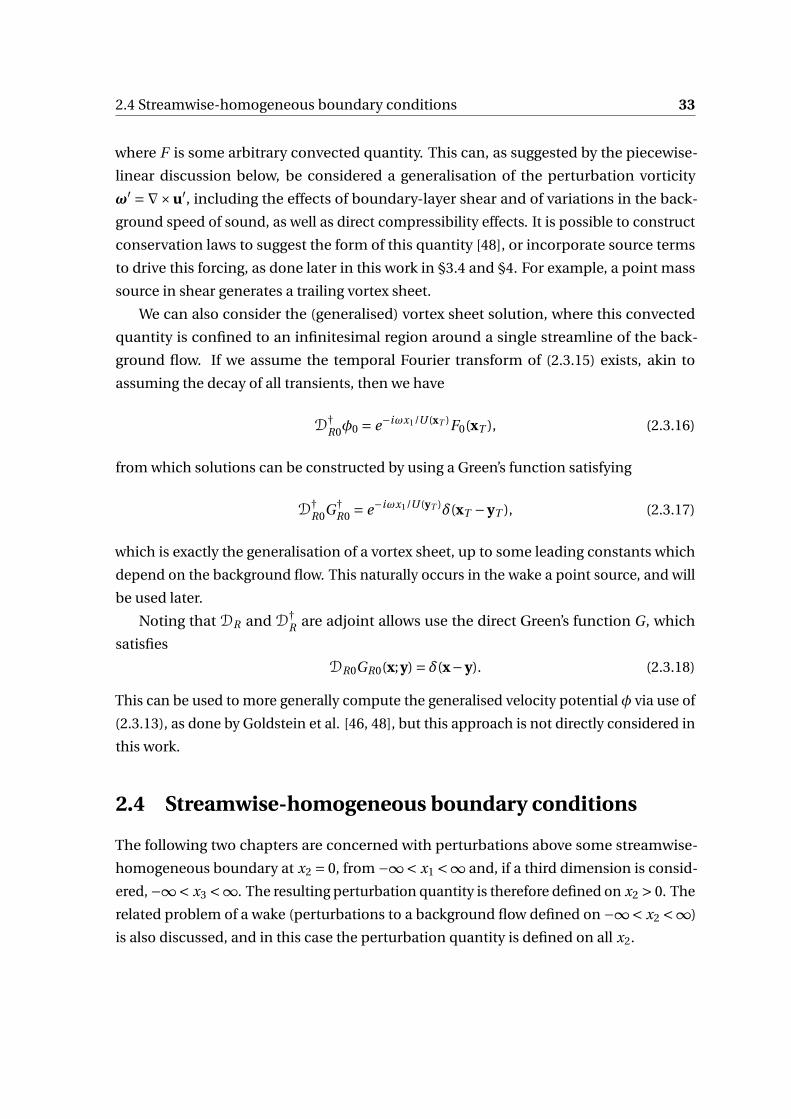
2.4 Streamwise-homogeneous boundary conditions 33

where F is some arbitrary convected quantity. This can, as suggested by the piecewise-

linear discussion below, be considered a generalisation of the perturbation vorticity

ω′ =∇×u′, including the effects of boundary-layer shear and of variations in the back-

ground speed of sound, as well as direct compressibility effects. It is possible to construct

conservation laws to suggest the form of this quantity [48], or incorporate source terms

to drive this forcing, as done later in this work in §3.4 and §4. For example, a point mass

source in shear generates a trailing vortex sheet.

We can also consider the (generalised) vortex sheet solution, where this convected

quantity is confined to an infinitesimal region around a single streamline of the back-

ground flow. If we assume the temporal Fourier transform of (2.3.15) exists, akin to

assuming the decay of all transients, then we have

D†R0φ0 = e−iωx1/U (xT )F0(xT ), (2.3.16)

from which solutions can be constructed by using a Green’s function satisfying

D†R0G†

R0 = e−iωx1/U (yT )δ(xT −yT ), (2.3.17)

which is exactly the generalisation of a vortex sheet, up to some leading constants which

depend on the background flow. This naturally occurs in the wake a point source, and will

be used later.

Noting that DR and D†R are adjoint allows use the direct Green’s function G , which

satisfies

DR0GR0(x;y) = δ(x−y). (2.3.18)

This can be used to more generally compute the generalised velocity potential φ via use of

(2.3.13), as done by Goldstein et al. [46, 48], but this approach is not directly considered in

this work.

2.4 Streamwise-homogeneous boundary conditions

The following two chapters are concerned with perturbations above some streamwise-

homogeneous boundary at x2 = 0, from −∞< x1 <∞ and, if a third dimension is consid-

ered, −∞< x3 <∞. The resulting perturbation quantity is therefore defined on x2 > 0. The

related problem of a wake (perturbations to a background flow defined on −∞< x2 <∞)

is also discussed, and in this case the perturbation quantity is defined on all x2.

34 Mathematical formulation of Rapid Distortion Theory

Causality. These problems involve a source being placed in the fluid, and the resulting

perturbations being investigated. It is important, therefore, to impose that all disturbances

are due to this source and have not come from outside the domain, for example waves

coming in from infinity, for which we refer to the introductory section §2.1. We impose

the Briggs-Bers stability criterion, by first considering large negative imaginary part of ω

to determine the direction of propagation of solutions.

Hard-wall and pressure release conditions. The simplest boundary condition is a hard-

wall boundary condition, where the fluid does not penetrate the wall, and is equivalent to

saying that the wall-normal velocity perturbation vanishes, i.e.

v ′(x2 = 0) = 0 (2.4.1)

We can also, similarly, consider pressure-release walls (which cannot support any pressure)

which instead simply have

p ′(x2 = 0) = 0 (2.4.2)

Lined wall. We can generalise by considering an impedance lining with both the hard-

wall and pressure release solutions a special case. Acoustic linings, used to reduce noise,

are typically modelled as a linear relationship between the wall-pressure and normal

velocity at the wall, with

Z (ω) = p ′

u′ ·n(2.4.3)

for harmonic disturbances proportional to exp(iωt). This must, however, be modified

if there is a slipping background flow, leading to the Ingard-Myers boundary condition

[61, 77], which considers fluid particle displacement as opposed to normal velocity, and

gives

iωZ (ω)u′ ·n = (iω+u0 ·∇− (n ·∇u0) ·n)p ′. (2.4.4)

For a straight wall, the final term is identically 0. Importantly, this gives a straightforward

linear relationship between v ′ (= u′ ·n) and p ′, which allows application of the usual

Fourier transform-based methods. The limit of large |Z | is exactly the hard-wall limit, and

the limit of vanishing Z the pressure-release limit (a wall that does not support force).

This work throughout focuses on harmonic disturbances, which is assumed to allow

treatment of the impedance, Z (ω), as a constant, since the physical ω is fixed. Whilst the

physical frequency is fixed, the mathematical choice of frequency is, however, allowed

to vary. When considering causality in the §??, the frequency was given an artificial

large, negative, imaginary part. This work assumes any variance in impedance with the

2.4 Streamwise-homogeneous boundary conditions 35

imaginary part of frequency does not affect any causality analysis, which is not necessarily

true. This is best observed by considering a simple mass-damper impedance model, with

impedance given by

Z (ω) = R + i dω− i b/ω. (2.4.5)

Even with the real part of frequency fixed for large Imω this impedance behaves like

−d Im(ω), which is fundamentally different from assuming Z does not depend on fre-

quency [19]. This could, for certain choice of parameters, change which complex half-

plane any modal disturbances lie in for large | Im(ω)|, which in turn changes their direction

of propagation as Im(ω) → 0. This caveat should be borne in mind by any readers, and the

author is very grateful to Professor S. Rienstra for highlighting this limitation.

Wake. Finally, the case of a background flow field U (x2) defined for all x2 ∈ (−∞,∞) will

be considered. While we assume this is everywhere continuous, we do not assume the

same condition holds on derivatives (for example, it is reasonable to suppose U ′(x2) is dis-

continuous at x2 = 0, which could for example represent a developed wake behind a plate,

on which the flow is smoothed out over some inner viscous lengthscale). Thus, as sug-

gested for junctions in §2.2.2, we impose continuity of velocity and pressure perturbations

across x2 = 0. Causality here dictates waves only propagate outwards for both x2 →±∞,

and it is this new condition at x2 →−∞ that fulfills the same role as the boundary in the

earlier examples.

If U (x2) =U∗(−x2) for x2 < 0, then under the transformation x2 7→ −x2 the differential

equation governing perturbations is unchanged, save for U being replaced by U∗. This

means that solutions on x2 < 0 can be computed as solutions on x2 > 0, without changing

any routines or methods, save substitution of the flow field. In particular this means

solutions with specified boundary conditions are identical under x2 7→ −x2 if the flow

profile is symmetric, U (x2) =U (−x2), which simplifies analysis.

Chapter 3

Long-wavelength disturbances to

piecewise-linear background flow

By considering small perturbations to some known background shear flow, the hydrody-

namic and acoustic behaviour of a point source, be it of mass, momentum or vorticity,

is considered as the perturbation evolves downstream. In this chapter, the simplified

case of long-wavelength disturbances to a piecewise-linearly sheared background flow

is considered, above a range of (streamwise-homogeneous) boundaries. This model is

developed and its strengths and limitations are discussed.

3.1 Introduction

The interaction of vortical motion within a turbulent boundary-layer with a sharp edge

of an aerofoil generates waves with acoustic wavelengths which radiate to the far-field

as noise. A sharp edge, or a discontinuity in the boundary condition on the surface of

the aerofoil, provides a strong mechanism to convert the hydrodynamic boundary-layer

turbulence into far-field noise, stronger than the normal quadrupole noise due to free

turbulence [34]. In practice, an incident turbulent wave, confined to a boundary-layer,

is modelled by a gust: a wavelike solution with particular frequency and wavenumber

propogating at a speed below the uniform free-stream velocity. The scattering of this wave,

from a sharp trailing-edge or other mixed boundary boundary conditions, can then be

solved using the Wiener-Hopf method.

This and the following chapter, §4, are focused on the understanding of the vortical

gust solution, in preparation for later scattering problems. The gust, confined to the

boundary-layer, critically depends on the shear inherent in the underlying flow. Infinitesi-

38 Long-wavelength disturbances to piecewise-linear background flow

mal disturbances to sheared flow is a classical problem stretching back to Lord Rayleigh

[84]. Orr [80] considered hydrodynamic disturbances to Couette flow in a pipe, that is

uniformly transversely sheared parallel flow, and the development of disturbances down-

stream. Noting inviscid two dimensional disturbances to linearly sheared background

flow U (x2) satisfy (∂

∂t+U (x2)

∂

∂x1

)ω′ = 0, (3.1.1)

with ω′ the perturbation vorticity, such that ∇×u′ =ω′e3, the solution is driven by vortical

solutions propogating with the mean velocity (i.e. dependent on time and streamwise

direction x1 only in the combination t −x1/U (x2)).

This simple setup can be used for considering acoustic problems and more compli-

cated background flow, through a long-wavelength approximation and consideration of

piecewise linear background shear. The long acoustic wavelength limit of the equations

derived by Goldstein [42] reproduce Orr’s equation in a thin region near boundaries, which

can in turn be matched to a radiating acoustic solution. As far as the acoustic motion is

concerned the boundary is compact and can therefore in a sense be ignored, in that a

sound wave propagating through an acoustically thin shear layer wouldn’t be modified by

the shear. However, both the gust setup and more careful treatment within this chapter

have sources within the boundary-layer, which therefore require an understanding of the

underlying acoustic behaviour within the boundary-layer itself.

Modelling a background flow as a continuous profile built from linear pieces has

multiple benefits. It results in analytically tractable solutions. Further, as noted by various

authors, (for example Heaton and Peake [50]), the presence of background vorticity mod-

ifies the acoustic problem, primarily through the need to consider a critical layer, with

the governing differential equations having a regular singular point when the streamwise

wavenumber k1 =ω/U (y2), for some y2 within the boundary-layer. The resulting branch

cut in the (complex) dispersion function D(k1,ω) might give rise to disturbances that

grow or decay only algebraically downstream. This problem is avoided solely in the case

that U ′′ = 0 above a flat plate (as opposed to, for example, within a cylindrical geometry),

almost exactly returning to the case considered by Orr. By considering a piecewise-linear

profile, with U ′′ = 0 everywhere except discrete points, the critical-layer is again of little

concern and the problem can be solved, to some extent, algebraically. This is the setup

used by Rienstra, Darau and Brambley [92] (hereafter RDB), who consider a point mass

source in infinite linear shear above a wall.

This chapter extends the results of RDB to a piecewise linear profile matched to uni-

form flow outside some boundary layer, and considers it as the inner problem to some

3.2 Rapid Distortion Theory in the long-wavelength limit 39

more general acoustic problem, through asymptotically matching to an acoustic solution

in uniform flow above this hypothetical boundary layer, using standard techniques [52].

This allows consideration of approximating more complicated background profiles with-

out removing all the mathematical niceties of this construction. Further, by considering

uniform flow outside some boundary-layer of finite thickness, issues of far-field conver-

gence in two dimensions, due to a perceived "infinite" far-field background flow, do not

occur. The following chapter will generalise these results to more complicated profiles,

and assess the suitability of this approximation.

Inclusion of realistic shear within a boundary-layer also allows another look at pertur-

bations above a lined wall [85, 89]. By considering a non-negligible boundary-layer of rea-

sonably arbitrary thickness this chapter allows analyses the imposition of an impedance

condition for slipping and non-slipping flow, avoiding some of the pitfalls of typical

uniform flow models, as previously done for a duct [22].

This chapter begins by simplifying the governing Rapid Distortion Theory equations

from the preceding chapter, §2. The problem of a point source above a surface with

streamwise-homogeneous boundary conditions is then considered, limited not only to a

hard-wall but more general boundary conditions (for example a lined wall) as well. Finally,

the evolution of disturbances in a wake is considered. These are primarily setting up

later chapters, via careful construction of the boundary-layer “gust” solution. Later we

will look at the scattering induced by a change from one boundary condition to another,

for which a complete understanding of boundary-layer solutions is useful. Further, this

chapter provides a straightforward model for boundary-layer noise, with limited numerical

complexity.

3.2 Rapid Distortion Theory in the long-wavelength limit

Motivated by RDB [92], we first consider the limit of long acoustic wavelength, for which

analytic progress can be made. For a harmonic solution proportional exp(iωt), we can

define an acoustic wavenumber

k0 = ω

c0. (3.2.1)

The wavelength of acoustic waves (which propagate with speed given by speed of sound c0)

is related to k0 asλa = 2π/k0, and so k−10 is a measure of the acoustic lengthscale. This gives

two lengthscales of interest for the problem, if the geometry of interest does not have any

lengthscales (such as the streamwise homogeneous case considered in this chapter, or with

semi-infinite streamwise boundary conditions considered in later scattering problems),

40 Long-wavelength disturbances to piecewise-linear background flow

namely the boundary-layer thickness δ, outside which the background flow is uniform,

and the acoustic lengthscale k−10 . This is physically appropriate for a large range of

frequencies and geometries. For k0δ≪ 1, we require

ω≪ c0

δ. (3.2.2)

If δ is on the order of centimetres, this approximation is valid provided ω≪ 104 s−1, which

covers a broad range of reasonably low, audible, frequencies.

We consider then the limit k0δ→ 0, which can be done in two ways: firstly by scaling

distances on the acoustic lengthscale k−10 , giving rise to an outer solution that doesn’t see

the boundary-layer at all, save in the imposition of boundary conditions; and secondly by

scaling distances on the boundary-layer lengthscale δ. The latter scaling (under certain

conditions on the Mach number) removes the majority of acoustic effects, and under

further assumptions allows analytic solution to the governing equations. The acoustics of

the problem then arise through matching to an appropriate outer solution.

3.2.1 Outer region

We firstly scale lengths with the reciprocal of (the real part of1) the acoustic wavenumber

k0 . We suppose that the timescale of evolution is ω−1 for some frequency ω, and use

this and the speed of sound at infinity with c0(x2) → c∞ as x2 →∞, to define an acoustic

wavenumber k0 =ω/c∞ and scale physical variables accordingly:

Ta =ωt (3.2.3a)

Xai = k0xi (3.2.3b)

Ma = U

c∞(3.2.3c)

ca = c0

c∞(3.2.3d)

which rescale Rayleigh’s equation (2.2.8) as Da

DTa

[D2

a

DT 2a−∇a · (c2

a∇a)

]+2c2

a∂Ma

∂Xa j

∂2

∂Xa1∂Xa j

p ′ = 0 (3.2.4)

1As outlined in the Briggs-Bers process in §2.1.2, we take the mathematical limit Im(ω) → 0− to under-stand causality, so ω and k0 might be complex. This does not occur physically in the final solution, so forscaling purposes we consider only the real part of ω and of k0.

3.2 Rapid Distortion Theory in the long-wavelength limit 41

where Da/DTa = ∂/∂Ta +M∂/∂Xa1 and ∇ai = ∂/∂Xai . The form of the equations is un-

changed. However, if we impose that U is uniform outside some boundary-layer confined

to x2 ∈ (0,δ), then∂Ma

∂Xa j

= 0 (3.2.5)

for Xa2 > δk0 → 0, i.e. almost everywhere in Xa space, save for a thin region near X2a = 0.

Thus, Rayleigh’s equation in the outer region is simply the convected wave equation[D2

a

DT 2a−∇2

a

]p ′ = 0. (3.2.6)

The superfluous convective derivative has been removed either by arguing there are no

sources within the outer region (where the flow is not turbulent) or by returning to the

original governing equations of momentum and mass-energy and noting the original

differentiation step is not required to remove the shear when there is no shear. We make

the further assumption that ca = 1 is constant outside the boundary-layer.

As suggested by the above, we cannot directly apply boundary conditions at Xa2 = 0,

since the shear need not be negligable there. Further, we expect acoustic sources to occur

within the boundary layer, which are not encapsulated by this limiting process.

3.2.2 Inner region

To deal with the near-wall region, we can scale with boundary-layer thickness δ as a

lengthscale, defining instead

Tb =ωt (3.2.7a)

Xbi =xi

δ(3.2.7b)

Ub = U

δω(3.2.7c)

cb = c0

c∞(3.2.7d)

and Rayleigh’s equation scales to Db

DTb

ϵ2D2

b

DT 2b

−∇b · (c2b∇b)

+2c2b

∂Ub

∂Xb j

∂2

∂Xb1∂Xb j

p ′ = 0 (3.2.8)

42 Long-wavelength disturbances to piecewise-linear background flow

with ϵ=ωδ/c∞ = k0δ, and the limiting process assumes that this is small. We can eliminate

the convective derivative in the square brackets provided the convection itself is not strong,

that the flow Mach number, Mb =Ub/c∞ is small for some representative Ub (e.g. at the

edge of the boundary-layer). Explicitly, if M 2b ≪ 1 we have the incompressible form of

Rayleigh’s equation: Db

DTb

[∇2

b

]−2

∂Ub

∂Xb j

∂2

∂Xb1∂Xb j

p ′ = 0, (3.2.9)

where we have made the further assumption that the speed of sound and the background

density ρ0 are constant within the boundary-layer, which is consistent with the assump-

tion of reasonably small Mb (as discussed in §2.1). We can thus define the linear differential

operator Di , the incompressible Rayleigh operator

Di = D0

Dt

[∇2

]−2

∂U

∂x j

∂2

∂x1∂x j. (3.2.10)

3.2.3 Alternative derivation of the equation in the inner region

This equation can be attained directly from the governing equations in the “limit” c0 →∞,

wherein the mass-energy equation reduces to

∇·u = 0. (3.2.11)

This is the expected expression for conservation of mass in an incompressible fluid.

Importantly this solenoidal property allows the velocity field u to be written as the curl of

a vector potential, and if the disturbance is two dimensional (and doesn’t depend on x3)

then this potential has a single component ψ′e3, with the streamfunction defined as usual

with

u′ = ∂ψ′

∂x2

, (3.2.12a)

v ′ =− ∂ψ′

∂x1

, (3.2.12b)

so that u′ = ∇× (ψ′e3). By instead eliminating pressure from the governing equations,

it is straightforward to get an equation governing the evolution of ψ′. The pressure is

most easily eliminated by taking the curl of the momentum equation (2.2.1b) to give the

3.2 Rapid Distortion Theory in the long-wavelength limit 43

vorticity equation (with density assumed constant throughout the fluid)

Dω

Dt−ω ·∇u = 0 (3.2.13)

The first term governs the change in vorticity ω = ∇×u as it is advected with the

flow, deforming purely through stretching by the fluid, encapsulated in the second term.

Linearised around a steady base flow u0, withω0 =∇×u0, this equation becomes

D0

Dtω′+u′ ·∇ω0 =ω0 ·∇u′+ω′ ·∇u0 (3.2.14)

with primes denoting perturbations around the mean flow as usual. We make the same

assumption as before, that u0 =U (x2, x3)e1, and make the further assumption that the

perturbation is entirely two dimensional (so that u′ is a function of x1 and x2 alone, and

has no x3 component, an assumption made purely to simplify the problem) which gives

ω′ =ω′e3. The third component of the vorticity equation (3.2.14) is then

D0ω′

Dt−u′

2∂2U

∂x22

= 0. (3.2.15)

The assumptions on the two-dimensional nature of the perturbation allow use of the

streamfunction discussed above, for which we have

D0

Dt

[∇2ψ′

]−U ′′(x2)

∂ψ′

∂x1

= 0, (3.2.16)

if we make the final simplification that U is a function of wall-normal coordinate x2 alone,

though this isn’t strictly necessary. This is the usual form of Rayleigh’s stability equation.

The resulting differential operator acting on ψ, Di , is given by

Di = D0

Dt

[∇2

]−U ′′ ∂

∂x1

. (3.2.17)

3.2.4 Linear shear

Most numerical difficulty in solving (2.2.8) arises from the singular nature of the ordinary

differential equation resulting from a spatial and temporal Fourier transform at points

with ω−U (x2)k1 = 0, when there is a regular singular point of the differential equation

for almost all choices of U . However, this difficulty disappears uniquely in the case that

U ′′ = 0. This can most obviously be seen (in the case c0 large) from the equation for the

streamfunction, (3.2.16), where the second term vanishes and we are simply left with an

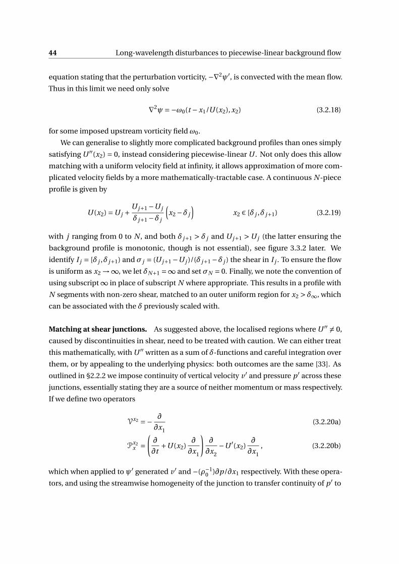
44 Long-wavelength disturbances to piecewise-linear background flow

equation stating that the perturbation vorticity, −∇2ψ′, is convected with the mean flow.

Thus in this limit we need only solve

∇2ψ=−ω0(t −x1/U (x2), x2) (3.2.18)

for some imposed upstream vorticity field ω0.

We can generalise to slightly more complicated background profiles than ones simply

satisfying U ′′(x2) = 0, instead considering piecewise-linear U . Not only does this allow

matching with a uniform velocity field at infinity, it allows approximation of more com-

plicated velocity fields by a more mathematically-tractable case. A continuous N -piece

profile is given by

U (x2) =U j +U j+1 −U j

δ j+1 −δ j

(x2 −δ j

)x2 ∈ [δ j ,δ j+1) (3.2.19)

with j ranging from 0 to N , and both δ j+1 > δ j and U j+1 > U j (the latter ensuring the

background profile is monotonic, though is not essential), see figure 3.3.2 later. We

identify I j = [δ j ,δ j+1) and σ j = (U j+1 −U j )/(δ j+1 −δ j ) the shear in I j . To ensure the flow

is uniform as x2 →∞, we let δN+1 =∞ and set σN = 0. Finally, we note the convention of

using subscript ∞ in place of subscript N where appropriate. This results in a profile with

N segments with non-zero shear, matched to an outer uniform region for x2 > δ∞, which

can be associated with the δ previously scaled with.

Matching at shear junctions. As suggested above, the localised regions where U ′′ = 0,

caused by discontinuities in shear, need to be treated with caution. We can either treat

this mathematically, with U ′′ written as a sum of δ-functions and careful integration over

them, or by appealing to the underlying physics: both outcomes are the same [33]. As

outlined in §2.2.2 we impose continuity of vertical velocity v ′ and pressure p ′ across these

junctions, essentially stating they are a source of neither momentum or mass respectively.

If we define two operators

Vx2 =− ∂

∂x1

(3.2.20a)

Px2x =

(∂

∂t+U (x2)

∂

∂x1

)∂

∂x2

−U ′(x2)∂

∂x1

, (3.2.20b)

which when applied to ψ′ generated v ′ and −(ρ−10 )∂p/∂x1 respectively. With these opera-

tors, and using the streamwise homogeneity of the junction to transfer continuity of p ′ to

3.3 Analytic solutions in the long-wavelength limit 45

continuity of its streamwise derivative, we can write the conditions at the junctions using

the notation in (2.2.11), namely[Vx2

0 ψ′]δ j

= [Px2

x 0ψ′]δ j

= 0. (3.2.21)

In the next section, we will transform in both time and the streamwise direction,

after which we obtain velocity and pressure operators (this time without the streamwise

derivative)

Vx201 = i k1, (3.2.22a)

Px2x01 =

1

i k1

(C (x2)

d

dx2

−C ′(x2)

), (3.2.22b)

with C = i (ω−Uk1) the transformed convective operator. The pressure operator is singular

for k1 = 0. This is a result of the x1-derivative in the definition, which leads to the choice

of an arbitrary x1-independent constant.

3.3 Analytic solutions in the long-wavelength limit

Exact solutions are permitted in the case of long wavelength and constant shear, where

the complete adjoint compressible Rayleigh equation reduces to

d2φ

dx22

+[

4C ′

C

]dφ

dx2

−(k2

1 +k23

)φ= 0, (3.3.1)

with C ′ = −i k1U ′ constant in x2 and C a simple linear function. This is extended by

considering piecewise linear shear, matching across discontinuities of U ′ as outlined

above. The resulting solutions can still be written down in terms of elementary functions,

though their representation is less simple.

Whilst (3.3.1) doesn’t obviously look like it has elementary solutions, we can use the

alternative formulation from §3.2 to derive them straightfowardly. A two-dimensional

solution has streamfunction satisfying (under streamwise transformation)(d2

dx22

−k21

)ψ01 = 0, (3.3.2)

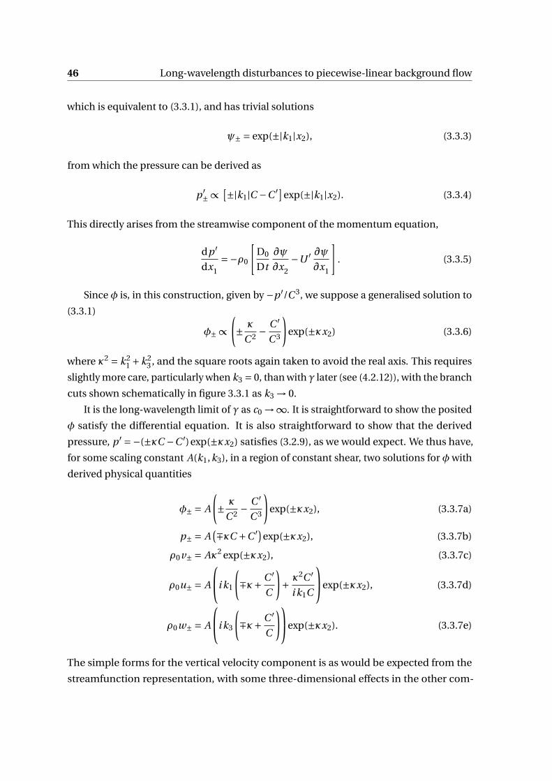
46 Long-wavelength disturbances to piecewise-linear background flow

which is equivalent to (3.3.1), and has trivial solutions

ψ± = exp(±|k1|x2), (3.3.3)

from which the pressure can be derived as

p ′± ∝ [±|k1|C −C ′]exp(±|k1|x2). (3.3.4)

This directly arises from the streamwise component of the momentum equation,

dp ′

dx1

=−ρ0

[D0

Dt

∂ψ

∂x2

−U ′ ∂ψ∂x1

]. (3.3.5)

Since φ is, in this construction, given by −p ′/C 3, we suppose a generalised solution to

(3.3.1)

φ± ∝(± κ

C 2− C ′

C 3

)exp(±κx2) (3.3.6)

where κ2 = k21 +k2

3 , and the square roots again taken to avoid the real axis. This requires

slightly more care, particularly when k3 = 0, than with γ later (see (4.2.12)), with the branch

cuts shown schematically in figure 3.3.1 as k3 → 0.

It is the long-wavelength limit of γ as c0 →∞. It is straightforward to show the posited

φ satisfy the differential equation. It is also straightforward to show that the derived

pressure, p ′ =−(±κC −C ′)exp(±κx2) satisfies (3.2.9), as we would expect. We thus have,

for some scaling constant A(k1,k3), in a region of constant shear, two solutions for φ with

derived physical quantities

φ± = A

(± κ

C 2− C ′

C 3

)exp(±κx2), (3.3.7a)

p± = A(∓κC +C ′)exp(±κx2), (3.3.7b)

ρ0v± = Aκ2 exp(±κx2), (3.3.7c)

ρ0u± = A

i k1

(∓κ+ C ′

C

)+ κ2C ′

i k1C

exp(±κx2), (3.3.7d)

ρ0w± = A

i k3

(∓κ+ C ′

C

)exp(±κx2). (3.3.7e)

The simple forms for the vertical velocity component is as would be expected from the

streamfunction representation, with some three-dimensional effects in the other com-

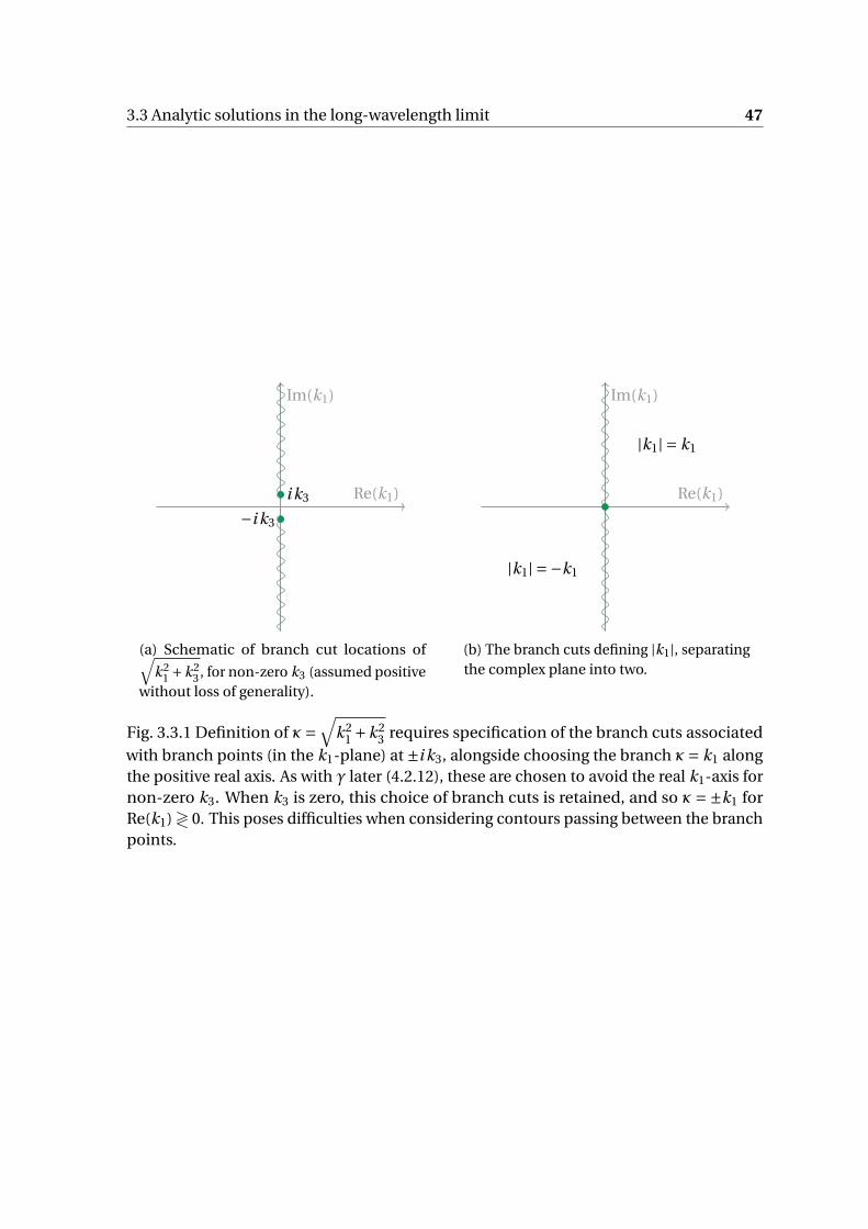
3.3 Analytic solutions in the long-wavelength limit 47

Re(k1)

Im(k1)

−i k3

i k3

(a) Schematic of branch cut locations of√k2

1 +k23 , for non-zero k3 (assumed positive

without loss of generality).

Re(k1)

Im(k1)

|k1| = k1

|k1| = −k1

(b) The branch cuts defining |k1|, separatingthe complex plane into two.

Fig. 3.3.1 Definition of κ=√

k21 +k2

3 requires specification of the branch cuts associatedwith branch points (in the k1-plane) at ±i k3, alongside choosing the branch κ= k1 alongthe positive real axis. As with γ later (4.2.12), these are chosen to avoid the real k1-axis fornon-zero k3. When k3 is zero, this choice of branch cuts is retained, and so κ=±k1 forRe(k1)≷ 0. This poses difficulties when considering contours passing between the branchpoints.

48 Long-wavelength disturbances to piecewise-linear background flow

ponents from allowing spanwise variation. If the disturbance is purely two-dimensional

(w ′ = 0, and no dependence on x3), we then have a streamfunction

ψ± = exp(±κx2), (3.3.7f)

arising if we choose A = i k1ρ0/κ2 =−ρ0/(i k1), and it will often be this quantity used in

place of φ, as it arises more naturally and has a simpler form.

3.3.1 Matching at shear junctions

Suppose that U ′ is discontinuous across x2 =χ2, for some χ2, so that U =U0 +σ1(x2 −χ2)

for x2 >χ2 (up to some upper value, that we are not interested in), and U =U0 +σ2(x2 −χ2) for x2 < χ2. Suppose further that we are looking for a specific solution to (the now

incompressible) Rayleigh’s equation, with

φ= A1e−κχ2φ++B1eκχ2φ− x2 >χ2

A2e−κχ2φ++B2eκχ2φ− x2 <χ2, (3.3.8)

and we would like to be able to determine A2 and B2 in terms of A1 and B1, or vice versa.

Since the flow profile has been chosen to be continuous, all we require is imposition of

continuity of vertical velocity and of pressure. We identify C1,2 = i (ω−U0k1) (both identi-

cal) and C ′1,2 =−iσ1,2k1 (discontinuous) and then the continuity conditions, respectively

of v ′ and p ′, become

A1 +B1 = A2 +B2 (3.3.9a)

(κC1 −C ′1)A1 + (−κC1 −C ′

1)B1 = (κC2 −C ′2)A2 + (−κC2 −C ′

2)B2. (3.3.9b)

We can write this in matrix form as M1A1 = M2A2 with A j = (A j ,B j ) and the matrices

(and their inverses) given by

M j = 1 1

κC j −C ′j −κC j −C ′

j

, M−1j = 1

2κC j

κC j +C ′j 1

κC j −C ′j −1

. (3.3.10)

With C1 =C2 ≡C0, the product S1 = M−11 M2 can be written in terms of a single quantity,

∆, defined as

∆= C ′1 −C ′

2

2κC0= k1(σ2 −σ1)

2κ(ω−U0k1)(3.3.11)

3.3 Analytic solutions in the long-wavelength limit 49

with

S1 = M−11 M2 =

1+∆ ∆

−∆ 1−∆

. (3.3.12)

A similar expression is obtained for S2 = M−12 M1 via ∆ 7→ −∆. With these, we have

A1 = S1A2, (3.3.13a)

A2 = S2A1. (3.3.13b)

From this we can construct analytic solutions for reasonably complicated, piecewise-

linear, background profiles.

3.3.2 Streamfunction for generic N -piece profile

Recall §3.2.4, where defined a generic, piecewise linear, background profile for x2 ≥ 0 as

U (x2) =U j +σ j x2 (3.3.14)

for x2 ∈ I j = [δ j ,δ j+1), and IN = [δN ,∞). Here, (δ0,δ1, ...,δN ) and (U0,U1, ...,UN ) are pre-

scribed parameters, with δ j > δ j−1 for all j . This setup is shown in figure 3.3.2, extended

to include negative j (which does little to the mathematics, but allows for more general

behaviour to be considered). The shear in each layer, σ j , is chosen to ensure continuity,

with

σ j =U j+1 −U j

δ j+1 −δ j(3.3.15)

for j = 0,1, . . . , N − 1, with σN = 0. We therefore have a piecewise linear profile with

U (δ j ) =U j and uniform background flow for x2 > δN ≡ δ∞, where U (x2) =UN ≡U∞. This

can easily be used to approximate more complicated profiles with line segments, though

the validity of this approximation is tested in this chapter.

For such a generic profile, we have solutions of the form

ψ(x2) = A jψ+(x2)+B jψ−(x2) x2 ∈ I j (3.3.16)

with only one pair of A j and B j to be prescribed, with the rest derived via the matching

formulae above.

We consider three solutions: the decaying solution, the solution with vanishing wall-

normal perturbation velocity on x2 = 0, and the solution with vanishing perturbation

pressure on x2 = 0. The former requires (with a choice of normalisation) AN = 0, BN = 1,

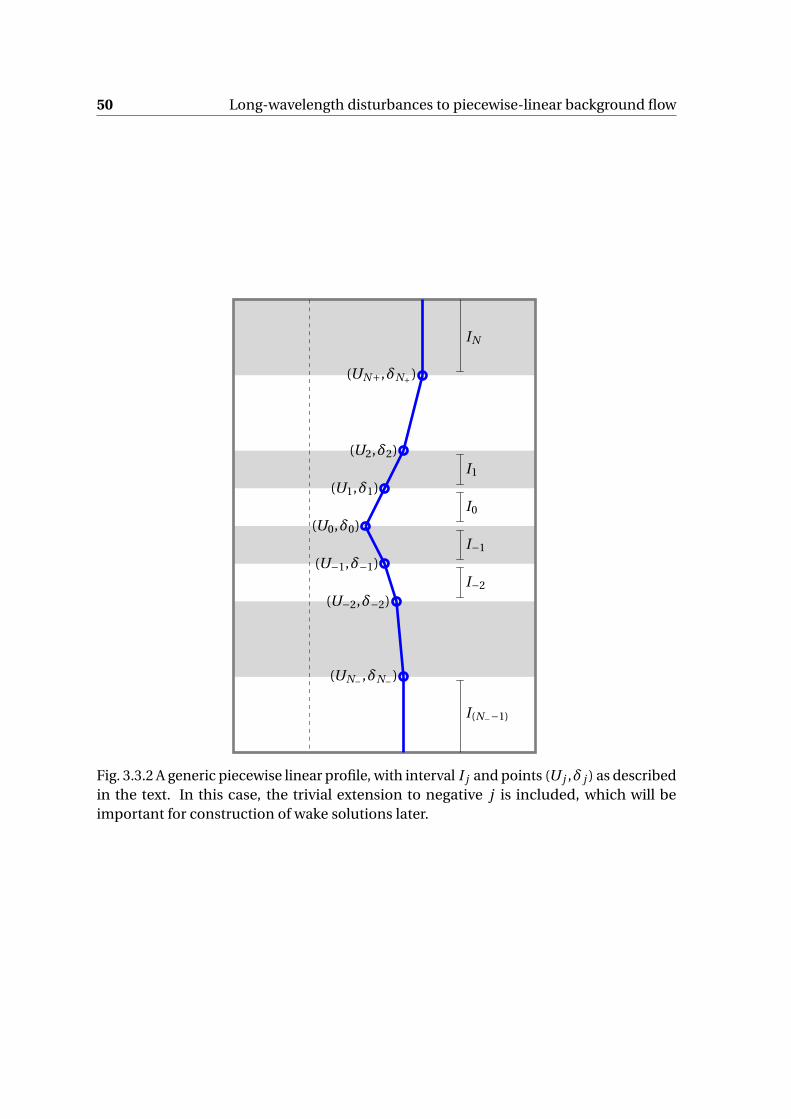
50 Long-wavelength disturbances to piecewise-linear background flow

(UN+,δN+)

(U2,δ2)

(U1,δ1)

(U0,δ0)

(U−1,δ−1)

(U−2,δ−2)

(UN− ,δN−)

IN

I1

I0

I−1

I−2

I(N−−1)

Fig. 3.3.2 A generic piecewise linear profile, with interval I j and points (U j ,δ j ) as describedin the text. In this case, the trivial extension to negative j is included, which will beimportant for construction of wake solutions later.

3.3 Analytic solutions in the long-wavelength limit 51

and will be denoted ψd . The latter two shall be denoted ψh (hard-wall) and ψp (pressure-

release) respectively and we have

ψh : A0 = 1

2κ; B0 =− 1

2κ(3.3.17a)

ψp : A0 =− C0

2C ′0

− 1

2κ; B0 =− C0

2C ′0

+ 1

2κ(3.3.17b)

with C0 = i(ω−U0k1

)and C ′

0 =−i k1σ0. Normalisation has been chosen so that ψ′h(x2 =

0) = 0 and ψp (x2 = 0) =−C0/C ′0, for reasons explained in later sections.

In some simple cases, it is possible to write down analytic expressions for the com-

plete functions, though for N even reasonably large it only makes sense to compute the

coefficients numerically, as the expressions for the case N = 2 suggest.

Single piece profile: N = 1. This case is completely prescribed by slip velocity U0 and

free-stream velocity U∞, with δ0 = 0 without loss of generality and boundary-layer thick-

ness δ1 = δ∞, and studied in detail by [96]. For ψd , we have

A0 =−∆1e−2κδ∞ , (3.3.18a)

B0 = (1+∆1). (3.3.18b)

For ψh we have

A1 = 1

2κ

(1+∆1 −∆1e−2κδ∞

), (3.3.19a)

B1 = 1

2κ

(∆1 −1−∆1e2κδ∞

). (3.3.19b)

Finally, for ψp we have

A1 =− 1

2κ

(1+∆1 −∆1e−2κδ∞

)− C0

2C ′0

(1+∆1 +∆1e−2κδ∞

), (3.3.20a)

B1 =− 1

2κ

(∆1 −1−∆1e2κδ∞

)− C0

2C ′0

(1−∆1 −∆1e2κδ∞

). (3.3.20b)

with, in all cases,∆1 defined analogously to∆ in the jump conditions derivation, evaluated

at x2 = δ1, namely

∆1 =C ′

1 −C ′0

2κC1= k1σ0

2κ(ω−U1k1)(3.3.21)

since there is no shear for x2 > δ1. This is singular when k1 =ω/U (δ1), which corresponds

to wavelike solutions moving at the free-stream velocity.

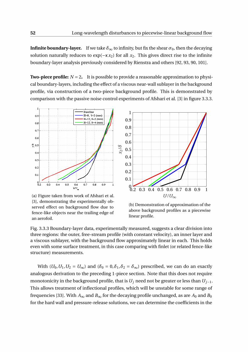
52 Long-wavelength disturbances to piecewise-linear background flow

Infinite boundary-layer. If we take δ∞ to infinity, but fix the shearσ0, then the decaying

solution naturally reduces to exp(−κx2) for all x2. This gives direct rise to the infinite

boundary-layer analysis previously considered by Rienstra and others [92, 93, 90, 101].

Two-piece profile: N = 2. It is possible to provide a reasonable approximation to physi-

cal boundary-layers, including the effect of a viscous near-wall sublayer in the background

profile, via construction of a two-piece background profile. This is demonstrated by

comparison with the passive noise control experiments of Afshari et al. [3] in figure 3.3.3.

(a) Figure taken from work of Afshari et al.[3], demonstrating the experimentally ob-served effect on background flow due tofence-like objects near the trailing edge ofan aerofoil.

0.2 0.3 0.4 0.5 0.6 0.7 0.8 0.9 10

0.1

0.2

0.3

0.4

0.5

0.6

0.7

0.8

0.9

1

U /U∞

x 2/δ

(b) Demonstration of approximation of theabove background profiles as a piecewiselinear profile.

Fig. 3.3.3 Boundary-layer data, experimentally measured, suggests a clear division intothree regions: the outer, free-stream profile (with constant velocity), an inner layer anda viscous sublayer, with the background flow approximately linear in each. This holdseven with some surface treatment, in this case comparing with finlet (or related fence-likestructure) measurements.

With (U0,U1,U2 = U∞) and (δ0 = 0,δ1,δ2 = δ∞) prescribed, we can do an exactly

analogous derivation to the preceding 1-piece section. Note that this does not require

monotonicity in the background profile, that is U j need not be greater or less than U j−1.

This allows treatment of inflectional profiles, which will be unstable for some range of

frequencies [33]. With A∞ and B∞ for the decaying profile unchanged, as are A0 and B0

for the hard wall and pressure-release solutions, we can determine the coefficients in the

3.4 A point source in sheared flow 53

other regions. For ψd , we have

A1 =−∆2e−2κδ2 , (3.3.22a)

B1 = (1+∆2), (3.3.22b)

A0 =−∆2(1−∆1)e−2κδ2 −∆1(1+∆2)e−2κδ1 , (3.3.22c)

B0 =−∆1∆2e2κ(δ1−δ2) + (1+∆1)(1+∆2). (3.3.22d)

For ψh we have

2κA1 = 1+∆1 −∆1e−2κδ1 , (3.3.23a)

2κB1 =−(1−∆1)−∆1e2κδ1 , (3.3.23b)

2κA2 = (1+∆1)(1+∆2)−∆1(1+∆2)e−2κδ1 − (1−∆1)∆2e−2κδ2 −∆1∆2e−2κ(δ2−δ1),

(3.3.23c)

2κB2 =−(1−∆1)(1−∆2)−∆1(1−∆2)e2κδ1 − (1+∆1)∆2e2κδ2 +∆2∆1e2κ(δ2−δ1). (3.3.23d)

The expression for ψp is omitted for brevity, but it can be similarly computed. As can be

seen, finding analytic expressions for these coefficients rapidly increases in difficulty with

the number of pieces involved, though all involve products of∆ j , (1±∆ j ) and exponentials

of the form exp(±κδ j ) and, other than scaling factors, no other terms.

3.4 A point source in sheared flow

Now we have determined a variety of ways of solving the long-wavelength limit of the

Rayleigh equation, we focus on using these solutions in a specific case: that of a point

source at some location in sheared flow, with a disturbance evolving downstream, above

some streamwise-homogeneous boundary. We begin by considering the long-wavelength

problem allowing treatment of the disturbance within the boundary-layer as incompress-

ible, matched to a compressible (acoustic) outer solution in the free-stream. This section

primarily focuses on the inner problem: two-dimensional disturbances to piecewise-

linear background flow with the governing equations set out in §3.2, slightly extended

to take into account a variety of upstream sources, either of mass or momentum at a

fixed location in the flow, or more generally a vortex sheet evolving from a fixed location.

The next chapter §4 will extend this analysis to the more general case of compressible

disturbances to continuously sheared background flow.

54 Long-wavelength disturbances to piecewise-linear background flow

3.4.1 Fixed mass or momentum source: Setup

Following RDB [92], we first consider the disturbances produced by a mass or momentum

source at some fixed location in the flow. This is done most readily by returning to the

(alternative) derivation of the governing equation for the streamfunction in the inner

region (see §3.2) and introducing source terms on the right-hand side of the mass and

momentum equations, namely

ρ∇·u = q, (3.4.1a)

ρDu

Dt+∇p = f. (3.4.1b)

The mass source q and momentum source f are potentially functions of time and space

(both per unit volume). If ρ = ρ(p) alone, as we expect under the earlier assumption of an

isotropic fluid, then ∇p ×∇ρ = 0. Then, upon taking the curl of the momentum equation

(3.4.1b) and substituting in (3.4.1a), gives the vorticity equation with source terms:

Dω

Dt−ω ·∇u =∇×

(f

ρ

)−ωq

ρ. (3.4.2)

Linearisation of a two-dimensional disturbance to parallel base flow U (x2)e1, as before,

givesD0ω

′

Dt−u′

2U ′′(x2) = ∂

∂x1

(f2

ρ

)− ∂

∂x2

(f1

ρ

)+ U ′q

ρ(3.4.3)

where we have assumed the mass and momentum source are the same order of magnitude

as the pertubation. For an N -piece piecewise linear flow, U ′′ = 0 (or, more generally,

U ′′ =∑Nj=1δ(x2 −x2 j ), with junctions at x2 j ) and so almost everywhere

D0

Dt∇2ψ′ = F (t ,x) (3.4.4)

with F (t ,x) =−U ′q/ρ−(∇×f/ρ)3. We consider a time-harmonic mass source 2, of strength

q0, concentrated at fixed location (0, y2), so that(iω+U

∂

∂x1

)∇2ψ′

0 =−U ′(y2)q0

ρ(y2)δ(x1)δ(x2 − y2) (3.4.5)

2Subscript 0 here denoting the (implicit) temporal Fourier transformation

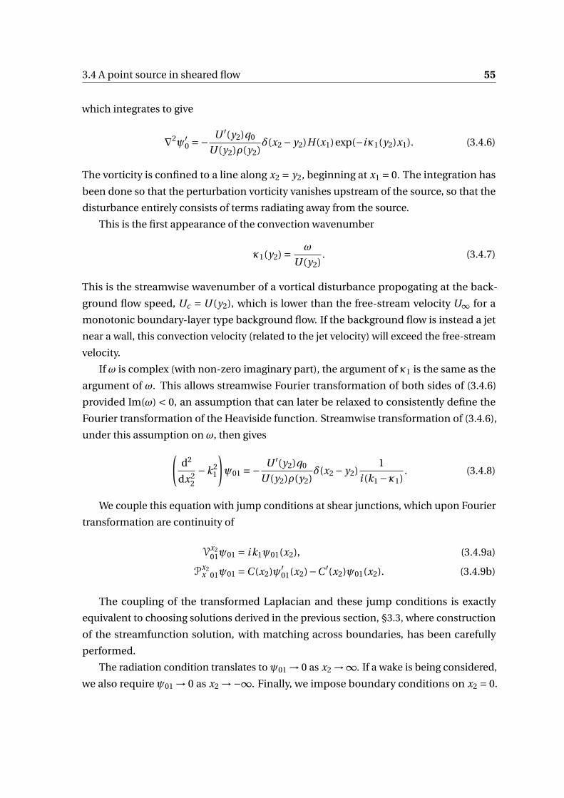
3.4 A point source in sheared flow 55

which integrates to give

∇2ψ′0 =− U ′(y2)q0

U (y2)ρ(y2)δ(x2 − y2)H(x1)exp(−iκ1(y2)x1). (3.4.6)

The vorticity is confined to a line along x2 = y2, beginning at x1 = 0. The integration has

been done so that the perturbation vorticity vanishes upstream of the source, so that the

disturbance entirely consists of terms radiating away from the source.

This is the first appearance of the convection wavenumber

κ1(y2) = ω

U (y2). (3.4.7)

This is the streamwise wavenumber of a vortical disturbance propogating at the back-

ground flow speed, Uc = U (y2), which is lower than the free-stream velocity U∞ for a

monotonic boundary-layer type background flow. If the background flow is instead a jet

near a wall, this convection velocity (related to the jet velocity) will exceed the free-stream

velocity.

If ω is complex (with non-zero imaginary part), the argument of κ1 is the same as the

argument of ω. This allows streamwise Fourier transformation of both sides of (3.4.6)

provided Im(ω) < 0, an assumption that can later be relaxed to consistently define the

Fourier transformation of the Heaviside function. Streamwise transformation of (3.4.6),

under this assumption on ω, then gives(d2

dx22

−k21

)ψ01 =− U ′(y2)q0

U (y2)ρ(y2)δ(x2 − y2)

1

i (k1 −κ1). (3.4.8)

We couple this equation with jump conditions at shear junctions, which upon Fourier

transformation are continuity of

Vx201ψ01 = i k1ψ01(x2), (3.4.9a)

Px2x 01ψ01 =C (x2)ψ′

01(x2)−C ′(x2)ψ01(x2). (3.4.9b)

The coupling of the transformed Laplacian and these jump conditions is exactly

equivalent to choosing solutions derived in the previous section, §3.3, where construction

of the streamfunction solution, with matching across boundaries, has been carefully

performed.

The radiation condition translates to ψ01 → 0 as x2 →∞. If a wake is being considered,

we also require ψ01 → 0 as x2 →−∞. Finally, we impose boundary conditions on x2 = 0.

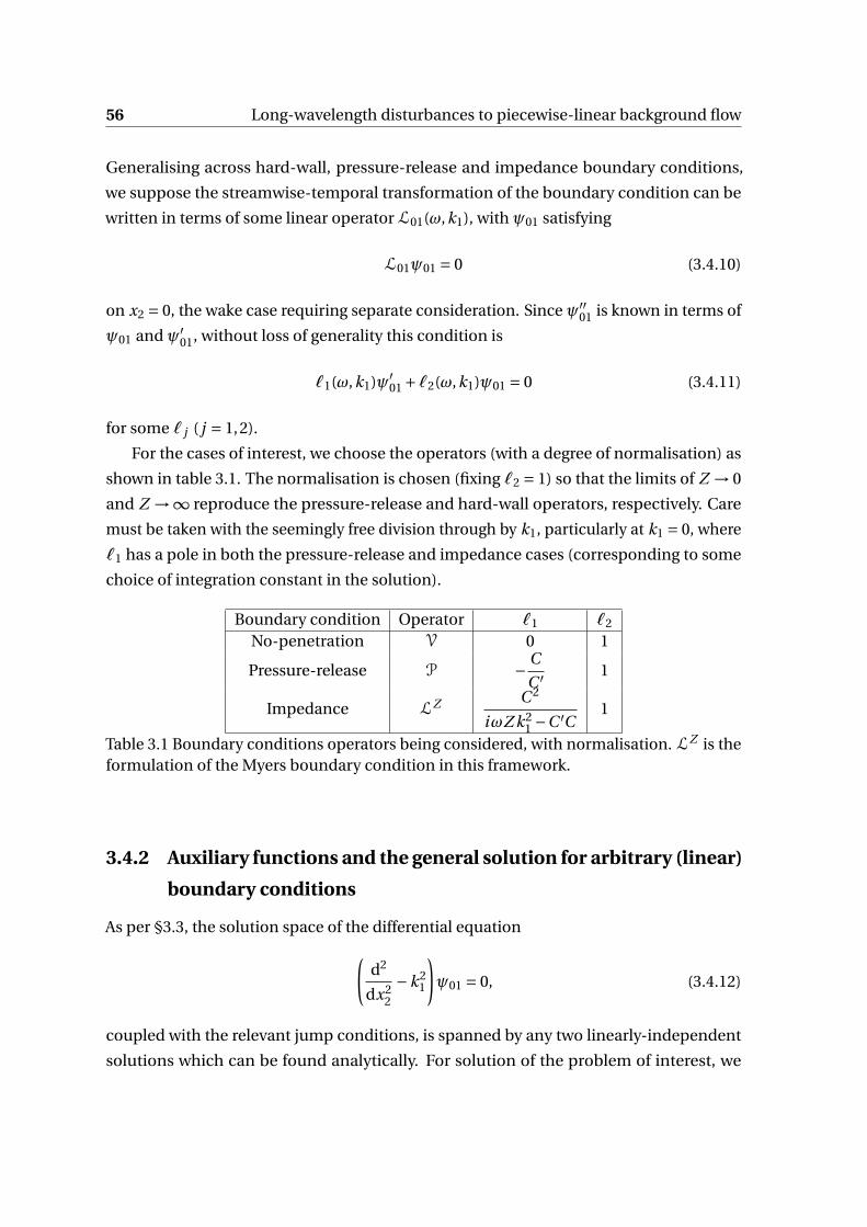
56 Long-wavelength disturbances to piecewise-linear background flow

Generalising across hard-wall, pressure-release and impedance boundary conditions,

we suppose the streamwise-temporal transformation of the boundary condition can be

written in terms of some linear operator L01(ω,k1), with ψ01 satisfying

L01ψ01 = 0 (3.4.10)

on x2 = 0, the wake case requiring separate consideration. Since ψ′′01 is known in terms of

ψ01 and ψ′01, without loss of generality this condition is

ℓ1(ω,k1)ψ′01 +ℓ2(ω,k1)ψ01 = 0 (3.4.11)

for some ℓ j ( j = 1,2).

For the cases of interest, we choose the operators (with a degree of normalisation) as

shown in table 3.1. The normalisation is chosen (fixing ℓ2 = 1) so that the limits of Z → 0

and Z →∞ reproduce the pressure-release and hard-wall operators, respectively. Care

must be taken with the seemingly free division through by k1, particularly at k1 = 0, where

ℓ1 has a pole in both the pressure-release and impedance cases (corresponding to some

choice of integration constant in the solution).

Boundary condition Operator ℓ1 ℓ2

No-penetration V 0 1

Pressure-release P − C

C ′ 1

Impedance LZ C 2

iωZ k21 −C ′C

1

Table 3.1 Boundary conditions operators being considered, with normalisation. LZ is theformulation of the Myers boundary condition in this framework.

3.4.2 Auxiliary functions and the general solution for arbitrary (linear)

boundary conditions

As per §3.3, the solution space of the differential equation(d2

dx22

−k21

)ψ01 = 0, (3.4.12)

coupled with the relevant jump conditions, is spanned by any two linearly-independent

solutions which can be found analytically. For solution of the problem of interest, we

3.4 A point source in sheared flow 57

choose two specific solutions: the decaying solution and the solution that satisfies the

boundary conditions of interest on x2 = 0. Explicitly, we normalise the decaying solution

ψd such that

ψd (x2) = exp(−|κ1|x2) x2 > δ∞, (3.4.13)

and we choose the wall solution ψℓ satisfying

L01ψℓ = 0 x2 = 0. (3.4.14)

There still remains a single degree of freedom in normalising this function, which will

be exploited later. Methods for explicitly writing down these auxiliary functions were

found in §3.3, utilising the fact that it is straightforward to solve (3.4.12) analytically, with

difficulty arising only from the matching conditions.

In terms of these functions, the solution to (3.4.8) is

ψ01(x2) =− U ′(y2)q0

U (y2)ρ(y2)

1

i (k1 −κ1)

1

W (y2)×

ψd (x2)ψℓ(y2) x2 > y2

ψℓ(x2)ψd (y2) x2 < y2. (3.4.15)

The Wronskian W = ψ′dψℓ−ψ′

ℓψd ensures the jump in derivative across x2 = y2 is as

expected (due to the δ function). Further, W is independent of its x2 (due to the lack of

first x2-derivative in (3.4.12) ) and can thus be evaluated at any point. Evaluating at x2 = 0,

where we recall ℓ1ψ′ℓ+ℓ2ψℓ = 0, we have

W (0) = ψℓ

ℓ1

(ℓ1ψ

′d +ℓ2ψd

)= ψℓ

ℓ1L01ψd , (3.4.16)

with all functions evaluated at x2 = 0. There is a degree of freedom with ψℓ, and thus we

choose ψℓ(0) = ℓ1. We now define the dispersion function for this boundary condition,

Dℓ(ω,k1), to be precisely the remaining part:

Dℓ =L01ψd (x2 = 0). (3.4.17)

Zeros of this function correspond to solutions to the differential equation that satisfy

the boundary conditions at both ∞ and at 0. Whilst these generally don’t exist, or are

trivial, for uniform flow, the presence of the boundary layer enriches the behaviour of the

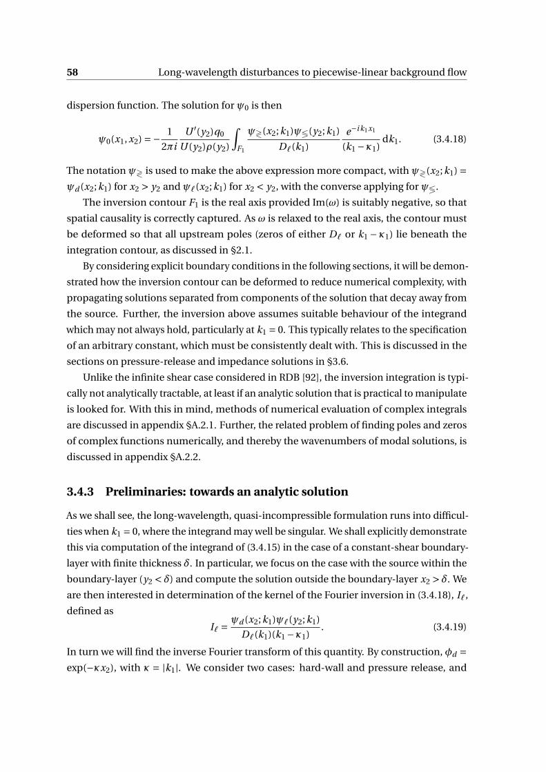
58 Long-wavelength disturbances to piecewise-linear background flow

dispersion function. The solution for ψ0 is then

ψ0(x1, x2) =− 1

2πi

U ′(y2)q0

U (y2)ρ(y2)

∫F1

ψ≷(x2;k1)ψ≶(y2;k1)

Dℓ(k1)

e−i k1x1

(k1 −κ1)dk1. (3.4.18)

The notation ψ≷ is used to make the above expression more compact, with ψ≷(x2;k1) =ψd (x2;k1) for x2 > y2 and ψℓ(x2;k1) for x2 < y2, with the converse applying for ψ≶.

The inversion contour F1 is the real axis provided Im(ω) is suitably negative, so that

spatial causality is correctly captured. As ω is relaxed to the real axis, the contour must

be deformed so that all upstream poles (zeros of either Dℓ or k1 −κ1) lie beneath the

integration contour, as discussed in §2.1.

By considering explicit boundary conditions in the following sections, it will be demon-

strated how the inversion contour can be deformed to reduce numerical complexity, with

propagating solutions separated from components of the solution that decay away from

the source. Further, the inversion above assumes suitable behaviour of the integrand

which may not always hold, particularly at k1 = 0. This typically relates to the specification

of an arbitrary constant, which must be consistently dealt with. This is discussed in the

sections on pressure-release and impedance solutions in §3.6.

Unlike the infinite shear case considered in RDB [92], the inversion integration is typi-

cally not analytically tractable, at least if an analytic solution that is practical to manipulate

is looked for. With this in mind, methods of numerical evaluation of complex integrals

are discussed in appendix §A.2.1. Further, the related problem of finding poles and zeros

of complex functions numerically, and thereby the wavenumbers of modal solutions, is

discussed in appendix §A.2.2.

3.4.3 Preliminaries: towards an analytic solution

As we shall see, the long-wavelength, quasi-incompressible formulation runs into difficul-

ties when k1 = 0, where the integrand may well be singular. We shall explicitly demonstrate

this via computation of the integrand of (3.4.15) in the case of a constant-shear boundary-

layer with finite thickness δ. In particular, we focus on the case with the source within the

boundary-layer (y2 < δ) and compute the solution outside the boundary-layer x2 > δ. We

are then interested in determination of the kernel of the Fourier inversion in (3.4.18), Iℓ,

defined as

Iℓ =ψd (x2;k1)ψℓ(y2;k1)

Dℓ(k1)(k1 −κ1). (3.4.19)

In turn we will find the inverse Fourier transform of this quantity. By construction, φd =exp(−κx2), with κ = |k1|. We consider two cases: hard-wall and pressure release, and

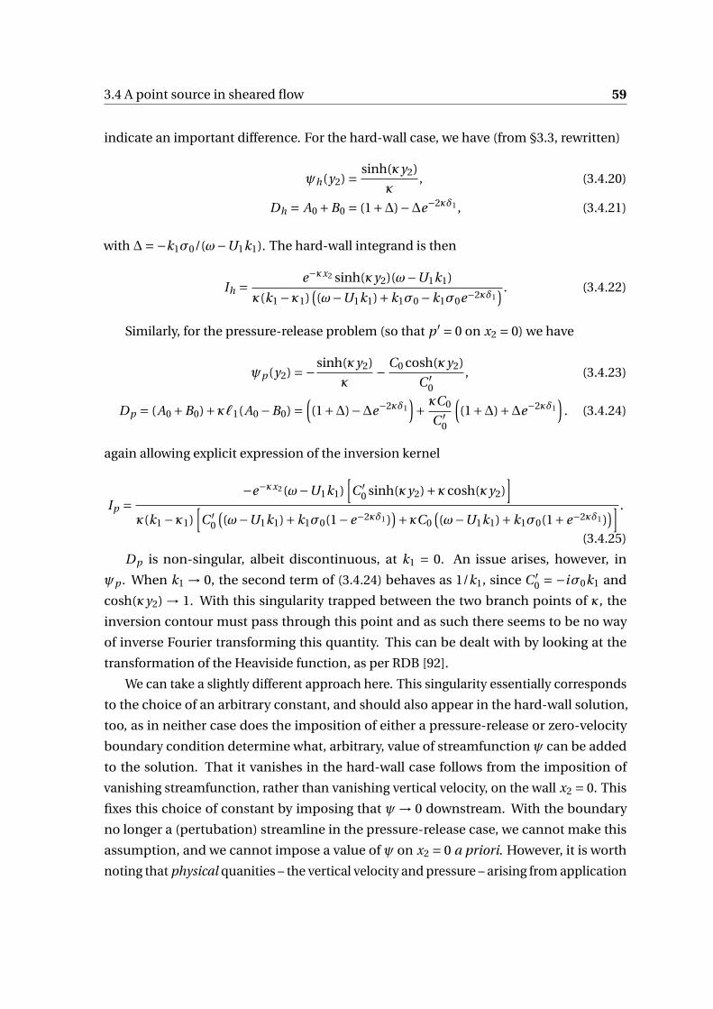
3.4 A point source in sheared flow 59

indicate an important difference. For the hard-wall case, we have (from §3.3, rewritten)

ψh(y2) = sinh(κy2)

κ, (3.4.20)

Dh = A0 +B0 = (1+∆)−∆e−2κδ1 , (3.4.21)

with ∆=−k1σ0/(ω−U1k1). The hard-wall integrand is then

Ih = e−κx2 sinh(κy2)(ω−U1k1)

κ(k1 −κ1)((ω−U1k1)+k1σ0 −k1σ0e−2κδ1

) . (3.4.22)

Similarly, for the pressure-release problem (so that p ′ = 0 on x2 = 0) we have

ψp (y2) =−sinh(κy2)

κ− C0 cosh(κy2)

C ′0

, (3.4.23)

Dp = (A0 +B0)+κℓ1(A0 −B0) =((1+∆)−∆e−2κδ1

)+ κC0

C ′0

((1+∆)+∆e−2κδ1

). (3.4.24)

again allowing explicit expression of the inversion kernel

Ip =−e−κx2 (ω−U1k1)

[C ′

0 sinh(κy2)+κcosh(κy2)]

κ(k1 −κ1)[C ′

0

((ω−U1k1)+k1σ0(1−e−2κδ1 )

)+κC0((ω−U1k1)+k1σ0(1+e−2κδ1 )

)] .

(3.4.25)

Dp is non-singular, albeit discontinuous, at k1 = 0. An issue arises, however, in

ψp . When k1 → 0, the second term of (3.4.24) behaves as 1/k1, since C ′0 = −iσ0k1 and

cosh(κy2) → 1. With this singularity trapped between the two branch points of κ, the

inversion contour must pass through this point and as such there seems to be no way

of inverse Fourier transforming this quantity. This can be dealt with by looking at the

transformation of the Heaviside function, as per RDB [92].

We can take a slightly different approach here. This singularity essentially corresponds

to the choice of an arbitrary constant, and should also appear in the hard-wall solution,

too, as in neither case does the imposition of either a pressure-release or zero-velocity

boundary condition determine what, arbitrary, value of streamfunction ψ can be added

to the solution. That it vanishes in the hard-wall case follows from the imposition of

vanishing streamfunction, rather than vanishing vertical velocity, on the wall x2 = 0. This

fixes this choice of constant by imposing that ψ→ 0 downstream. With the boundary

no longer a (pertubation) streamline in the pressure-release case, we cannot make this

assumption, and we cannot impose a value of ψ on x2 = 0 a priori. However, it is worth

noting that physical quanities – the vertical velocity and pressure – arising from application

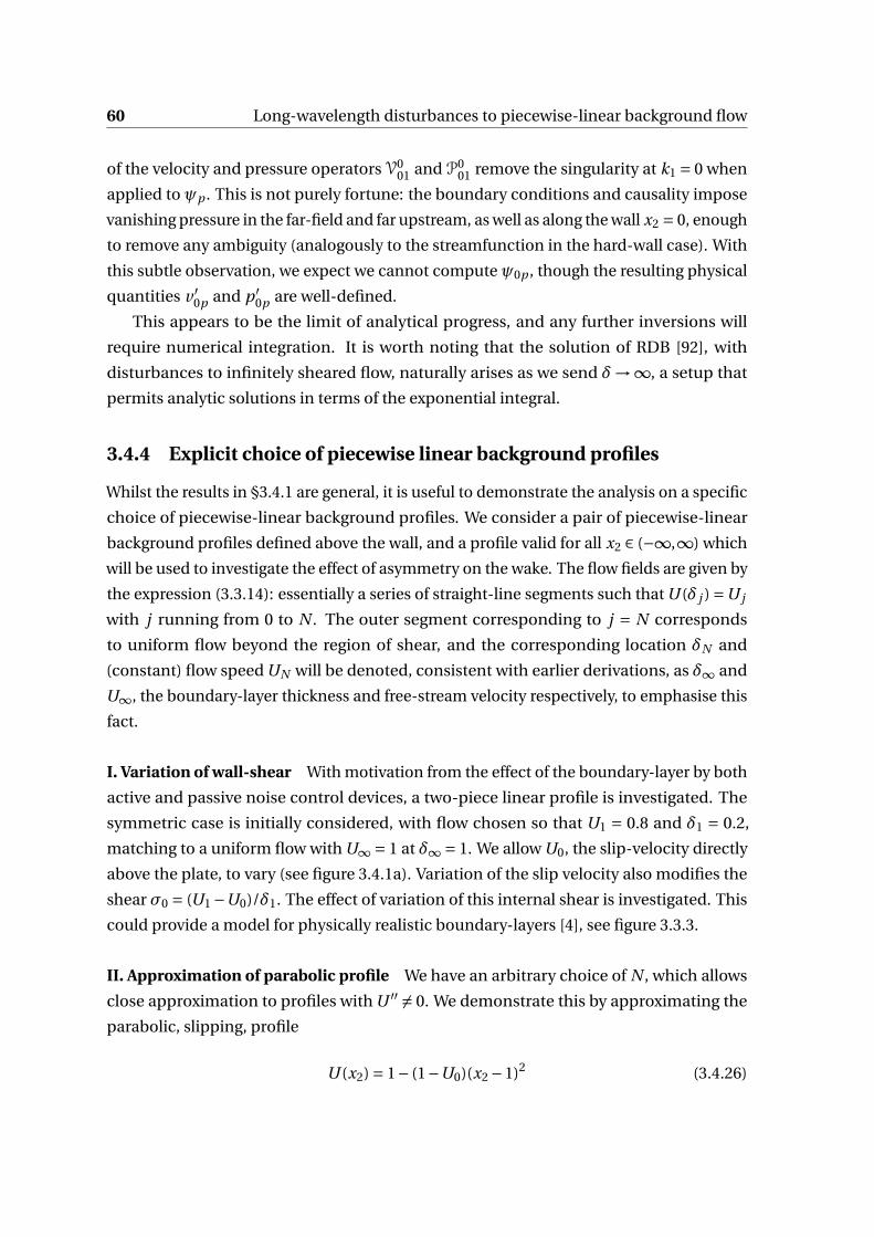
60 Long-wavelength disturbances to piecewise-linear background flow

of the velocity and pressure operators V001 and P0

01 remove the singularity at k1 = 0 when

applied to ψp . This is not purely fortune: the boundary conditions and causality impose

vanishing pressure in the far-field and far upstream, as well as along the wall x2 = 0, enough

to remove any ambiguity (analogously to the streamfunction in the hard-wall case). With

this subtle observation, we expect we cannot compute ψ0p , though the resulting physical

quantities v ′0p and p ′

0p are well-defined.

This appears to be the limit of analytical progress, and any further inversions will

require numerical integration. It is worth noting that the solution of RDB [92], with

disturbances to infinitely sheared flow, naturally arises as we send δ→∞, a setup that

permits analytic solutions in terms of the exponential integral.

3.4.4 Explicit choice of piecewise linear background profiles

Whilst the results in §3.4.1 are general, it is useful to demonstrate the analysis on a specific

choice of piecewise-linear background profiles. We consider a pair of piecewise-linear

background profiles defined above the wall, and a profile valid for all x2 ∈ (−∞,∞) which

will be used to investigate the effect of asymmetry on the wake. The flow fields are given by

the expression (3.3.14): essentially a series of straight-line segments such that U (δ j ) =U j

with j running from 0 to N . The outer segment corresponding to j = N corresponds

to uniform flow beyond the region of shear, and the corresponding location δN and

(constant) flow speed UN will be denoted, consistent with earlier derivations, as δ∞ and

U∞, the boundary-layer thickness and free-stream velocity respectively, to emphasise this

fact.

I. Variation of wall-shear With motivation from the effect of the boundary-layer by both

active and passive noise control devices, a two-piece linear profile is investigated. The

symmetric case is initially considered, with flow chosen so that U1 = 0.8 and δ1 = 0.2,

matching to a uniform flow with U∞ = 1 at δ∞ = 1. We allow U0, the slip-velocity directly

above the plate, to vary (see figure 3.4.1a). Variation of the slip velocity also modifies the

shear σ0 = (U1 −U0)/δ1. The effect of variation of this internal shear is investigated. This

could provide a model for physically realistic boundary-layers [4], see figure 3.3.3.

II. Approximation of parabolic profile We have an arbitrary choice of N , which allows

close approximation to profiles with U ′′ = 0. We demonstrate this by approximating the

parabolic, slipping, profile

U (x2) = 1− (1−U0)(x2 −1)2 (3.4.26)

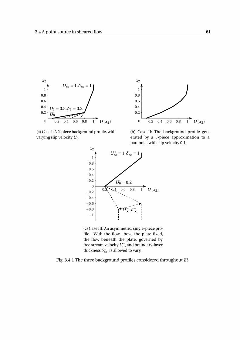
3.4 A point source in sheared flow 61

U (x2)0.2 0.4 0.6 0.8 1

x2

0.2

0.4

0.6

0.8

1

0

U∞ = 1,δ∞ = 1

U1 = 0.8,δ1 = 0.2U0

(a) Case I: A 2-piece background profile, withvarying slip velocity U0.

U (x2)0.2 0.4 0.6 0.8 1

x2

0.2

0.4

0.6

0.8

1

0

(b) Case II: The background profile gen-erated by a 5-piece approximation to aparabola, with slip velocity 0.1.

U (x2)0.2 0.4 0.6 0.8 1

x2

−1

−0.8

−0.6

−0.4

−0.2

0

0.2

0.4

0.6

0.8

1U+∞ = 1,δ+∞ = 1

U0 = 0.2

U−∞,δ−∞

(c) Case III: An asymmetric, single-piece pro-file. With the flow above the plate fixed,the flow beneath the plate, governed byfree stream velocity U−∞ and boundary-layerthickness δ−∞, is allowed to vary.

Fig. 3.4.1 The three background profiles considered throughout §3.

62 Long-wavelength disturbances to piecewise-linear background flow

for x2 < 1. This has slip velocity U (0) = U0, by construction. By letting δ j = j /N and

U j =U (δ j ), we obtain a N -piece approximation to this profile, in terms of linear pieces.

Increasing N leads to richer behaviour of the dispersion functions, which makes certain

facets of noise generation clearer. Here, we shall primarily consider the case N = 5, fixing

U0 = 0.1, as shown in figure 3.4.1b.

III. Wake asymmetry This model allows consideration of an asymmetric profile. With

this in mind, we consider a pair of single-piece profiles, above and below x2 = 0. This

gives three parameters that can be varied – the slip velocity U0 (which is assumed the

same above and below the plate, as continuity across the wake is required), as well as the

boundary-layer thickness below the plate, δ−, and the free-stream velocity below the plate

U−∞. For precision, we fix U0 = 0.2 and allow the other two parameters to vary, shown in

figure 3.4.1c.

3.5 Fixed mass or momentum source: Hard-wall

The hard-wall case is the most straightforward to consider, with fewer issues of stability to

worry about. As well as physically being the most important case, considering for example

a point source above the surface of a rigid aerofoil, it allows illustration of the numerical

methods which will be used in the more complicated lined cases in the next section, §3.6.

The hard-wall case arises from setting Lh01 =V0

01, so that ℓ1 = 0 and ℓ2 = i k1. However, we

can simplify further by instead letting

Lh01ψ=ψ (3.5.1)

so that ℓ2 = 1. This has been alluded to in both §3.3 and in §3.4.1, and is equivalent to,

instead of insisting that v ′ = 0 on x2 = 0, that x2 = 0 corresponds to the streamline ψ= 0.

This fixes a choice of arbitrary constant inψ, however it is valid as there is nothing stopping

the imposition that ψ→ 0 as x1 →−∞, since there is no perturbation far upstream. This

choice eliminates difficulties that arise at k1 = 0. With this, we have ψh the auxiliary

function that vanishes on x2 = 0, with ψ′h(x2 = 0) = 1 replicating the normalisation that

lead to (3.4.17). We label the corresponding dispersion function Dℓ→ Dh , explicitly

Dh(ω,k1) =ψd (0;ω,k1). (3.5.2)

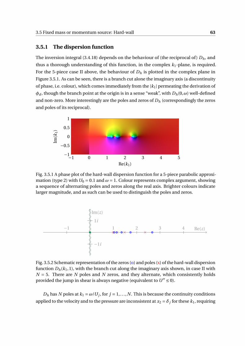
3.5 Fixed mass or momentum source: Hard-wall 63

3.5.1 The dispersion function

The inversion integral (3.4.18) depends on the behaviour of (the reciprocal of) Dh , and

thus a thorough understanding of this function, in the complex k1-plane, is required.

For the 5-piece case II above, the behaviour of Dh is plotted in the complex plane in

Figure 3.5.1. As can be seen, there is a branch cut alone the imaginary axis (a discontinuity

of phase, i.e. colour), which comes immediately from the |k1| permeating the derivation of

φd , though the branch point at the origin is in a sense “weak”, with Dh(0,ω) well-defined

and non-zero. More interestingly are the poles and zeros of Dh (correspondingly the zeros

and poles of its reciprocal).

−1 0 1 2 3 4 5−1

−0.5

0

0.5

1

Re(k1)

Im(k

1)

Fig. 3.5.1 A phase plot of the hard-wall dispersion function for a 5-piece parabolic approxi-mation (type 2) with U0 = 0.1 and ω= 1. Colour represents complex argument, showinga sequence of alternating poles and zeros along the real axis. Brighter colours indicatelarger magnitude, and as such can be used to distinguish the poles and zeros.

Re(z)

Im(z)

−1 1 2 3 4

−1i

1i

Fig. 3.5.2 Schematic representation of the zeros (o) and poles (x) of the hard-wall dispersionfunction Dh(k1,1), with the branch cut along the imaginary axis shown, in case II withN = 5. There are N poles and N zeros, and they alternate, which consistently holdsprovided the jump in shear is always negative (equivalent to U ′′ ≤ 0).

Dh has N poles at k1 =ω/U j , for j = 1, . . . , N . This is because the continuity conditions

applied to the velocity and to the pressure are inconsistent at x2 = δ j for these k1, requiring

64 Long-wavelength disturbances to piecewise-linear background flow

both φ and U ′φ to be continuous. It is practical and straightforward to remove these poles

by defining a reduced dispersion function

Dh(k1,ω) = R(k1,ω)Dh(k1,ω) (3.5.3)

with

R(k1,ω) =N∏

j=1

(k1 −ω/U j

). (3.5.4)

The resulting dispersion function is analytic everywhere in the complex plane, away from

the branch cuts along the imaginary axis.

For small k1, the jump conditions simply reduce to continuity of φ and φ′, with the

condition of continuity of pressure being asymptotically unaffected by the jump in shear

and as such the decaying solution reduces to exp(−κx2) as in the uniform case, and

Dh(k1) → 1 as k1 → 0.

A similar argument can be made for large k1. With all solutions the summation of

terms like exp(±|k1|x2), the +-term dominates for large k1 and therefore the derivative

ψ′ ∼ |k1|ψ, which indicatesψ′ andψmust be continuous as above. This can be determined

alternatively by directly considering the analytic expressions for A0 +B0 as k1 →∞. Due

to the exponential decay of most terms in the matching formulae, we have

Dh ∼ B0 ∼ (1+∆1)(1+∆2)...(1+∆N ) (3.5.5)

and all ∆ decay (as 1/k1) in the limit k1 →∞. The above approximation is very good for a

large range of k1, due to the exponential decay of all other terms as k1 increases.

Finally, and most interestingly, there are zeros of Dh , roots of the dispersion relation

Dh = 0. These contribute to the downstream Fourier inversion of the mass source, and

thus a complete understanding of them is desirable. Typically there are as many of these

zeros as poles, a claim discussed in the appendix, §A.1. These correspond to disturbances

convected with the flow. Provided the flow profile is concave, that is the shear in each layer

decreases with x2, these are real for real ω and are thus neutrally stable, essentially an

application of Rayleigh’s stability criterion, that a non-inflecting, parallel incompressible

flow is stable [33]. The poles and zeros for case II (a parabolic approximation), with

U0 = 0.1 and N = 5, are shown schematically Figure 3.5.2.

3.5 Fixed mass or momentum source: Hard-wall 65

3.5.2 Fourier inversion

Whilst analytic expressions for all terms in (3.4.18) can be determined, inversion of the

Fourier transform evades closed-form evaluation in anything but the most simple cases. In

practice, it is done numerically. We recall that the Fourier transforms are defined only for

ω with negative imaginary part, so that transforms of, for example, the Heaviside function

exist. However, if we relax Im(ω) → 0 and deform the Fourier inversion contour so that

there is no large change to the behaviour of the solution, we have an integral solution that

is valid even for real ω, displayed in Figure 3.5.3.

To invert, we deform the inversion contour onto the branch cuts, or more generally

into the upper and lower half planes for x1 respectively less than or greater than 0, shown

schematically in figure 3.5.4. This allows the integral to be decomposed into a rapidly

spatially decaying integral and a sum of residual contributions from poles, which corre-

spond to roots of the dispersion relation (and of the Cauchy-type kernel). Recall (3.4.18),

defining Q(y2) = q0U ′(y2)/(U (y2)ρ(y2)). For the hard-wall case we have

ψ0(x1, x2) =−Q(y2)

2πi

∫F1

Ψ(k1)e−i k1x1 dk1, (3.5.6)

where the Fourier transformed functionΨ(k1) =ψ01(k1) is

Ψ(k1) = ψ≷(x2;k1)ψ≶(y2;k1)

Dh(k1)

1

(k1 −κ1), (3.5.7)

for x2 ≷ y2, with ψ> =ψd and ψ< =ψh . Deforming F1 off the real axis, onto branch-cut

contours CU ,L in the upper- and lower-half complex planes (as per figure 3.5.4), respec-

tively, allows this to be written as

ψ0(x1, x2) =− Q

2πi

∫CU

Ψ(k1)e−i k1x1 dk1 (3.5.8)

for x1 < 0, for which there are no pole contributions (for U > 0). For x1 > 0, we have

ψ0(x1, x2) =− Q

2πi

∫CL

Ψ(k1)e−i k1x1 dk1 +Q

N∑j=1

ResΨ(k1 j )e−i k1 j x1 +ResΨ(κ1)e−iκ1x1

.

(3.5.9)

The residue of f at a (simple3) pole a defined in the usual way as Res f (a) = limz→a(z −a) f (z). The zeros of the dispersion relation k1 j give rise to a selection of neutrally stable

3Poles of the integrand, or zeros of the dispersion relationship, are assumed to be simple. This will betrue unless the parameters are chosen such that two poles are coincident, which occurs at the boundaries ofstability.

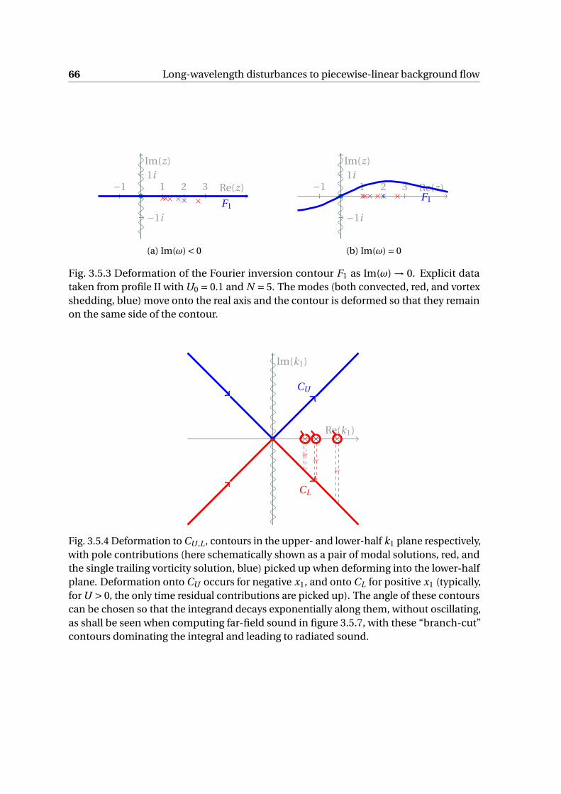
66 Long-wavelength disturbances to piecewise-linear background flow

Re(z)

Im(z)

−1 1 2 3

−1i

1i

F1

(a) Im(ω) < 0

Re(z)

Im(z)

−1 1 2 3

−1i

1i

F1

(b) Im(ω) = 0

Fig. 3.5.3 Deformation of the Fourier inversion contour F1 as Im(ω) → 0. Explicit datataken from profile II with U0 = 0.1 and N = 5. The modes (both convected, red, and vortexshedding, blue) move onto the real axis and the contour is deformed so that they remainon the same side of the contour.

Re(k1)

Im(k1)

CU

CL

Fig. 3.5.4 Deformation to CU ,L , contours in the upper- and lower-half k1 plane respectively,with pole contributions (here schematically shown as a pair of modal solutions, red, andthe single trailing vorticity solution, blue) picked up when deforming into the lower-halfplane. Deformation onto CU occurs for negative x1, and onto CL for positive x1 (typically,for U > 0, the only time residual contributions are picked up). The angle of these contourscan be chosen so that the integrand decays exponentially along them, without oscillating,as shall be seen when computing far-field sound in figure 3.5.7, with these “branch-cut”contours dominating the integral and leading to radiated sound.

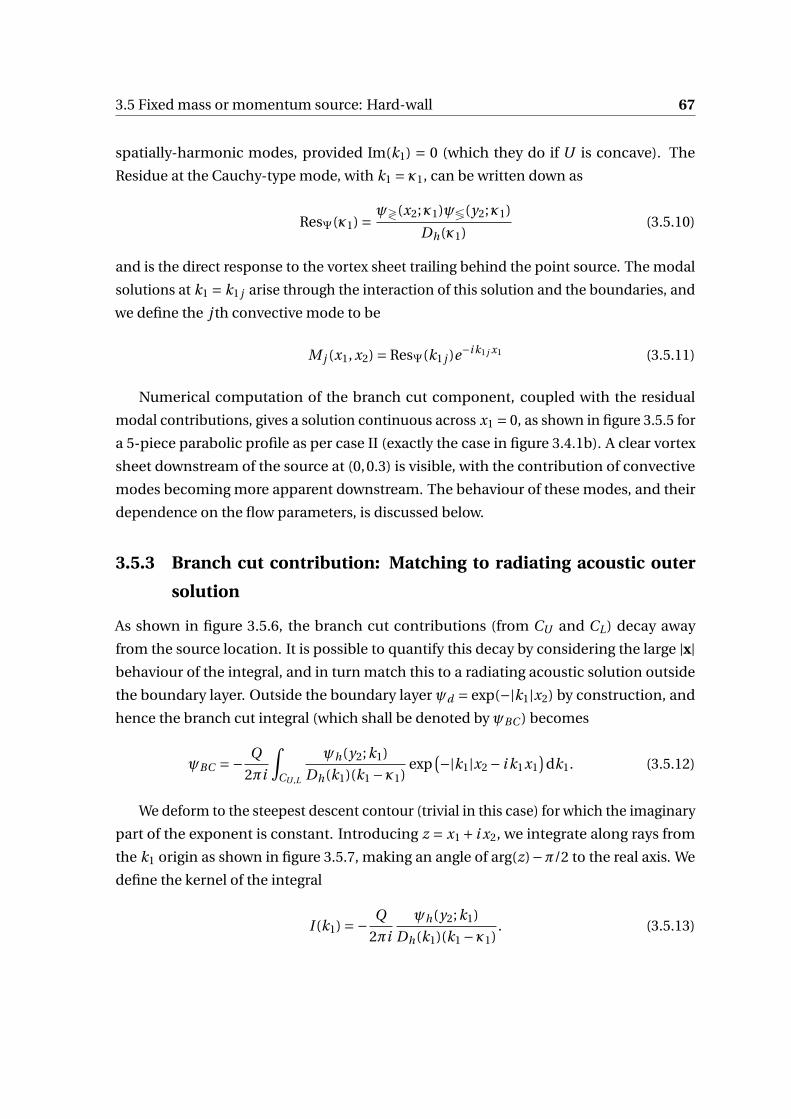
3.5 Fixed mass or momentum source: Hard-wall 67

spatially-harmonic modes, provided Im(k1) = 0 (which they do if U is concave). The

Residue at the Cauchy-type mode, with k1 = κ1, can be written down as

ResΨ(κ1) = ψ≷(x2;κ1)ψ≶(y2;κ1)

Dh(κ1)(3.5.10)

and is the direct response to the vortex sheet trailing behind the point source. The modal

solutions at k1 = k1 j arise through the interaction of this solution and the boundaries, and

we define the j th convective mode to be

M j (x1, x2) = ResΨ(k1 j )e−i k1 j x1 (3.5.11)

Numerical computation of the branch cut component, coupled with the residual

modal contributions, gives a solution continuous across x1 = 0, as shown in figure 3.5.5 for

a 5-piece parabolic profile as per case II (exactly the case in figure 3.4.1b). A clear vortex

sheet downstream of the source at (0,0.3) is visible, with the contribution of convective

modes becoming more apparent downstream. The behaviour of these modes, and their

dependence on the flow parameters, is discussed below.

3.5.3 Branch cut contribution: Matching to radiating acoustic outer

solution

As shown in figure 3.5.6, the branch cut contributions (from CU and CL) decay away

from the source location. It is possible to quantify this decay by considering the large |x|behaviour of the integral, and in turn match this to a radiating acoustic solution outside

the boundary layer. Outside the boundary layer ψd = exp(−|k1|x2) by construction, and

hence the branch cut integral (which shall be denoted by ψBC ) becomes

ψBC =− Q

2πi

∫CU ,L

ψh(y2;k1)

Dh(k1)(k1 −κ1)exp

(−|k1|x2 − i k1x1)

dk1. (3.5.12)

We deform to the steepest descent contour (trivial in this case) for which the imaginary

part of the exponent is constant. Introducing z = x1 + i x2, we integrate along rays from

the k1 origin as shown in figure 3.5.7, making an angle of arg(z)−π/2 to the real axis. We

define the kernel of the integral

I (k1) =− Q

2πi

ψh(y2;k1)

Dh(k1)(k1 −κ1). (3.5.13)

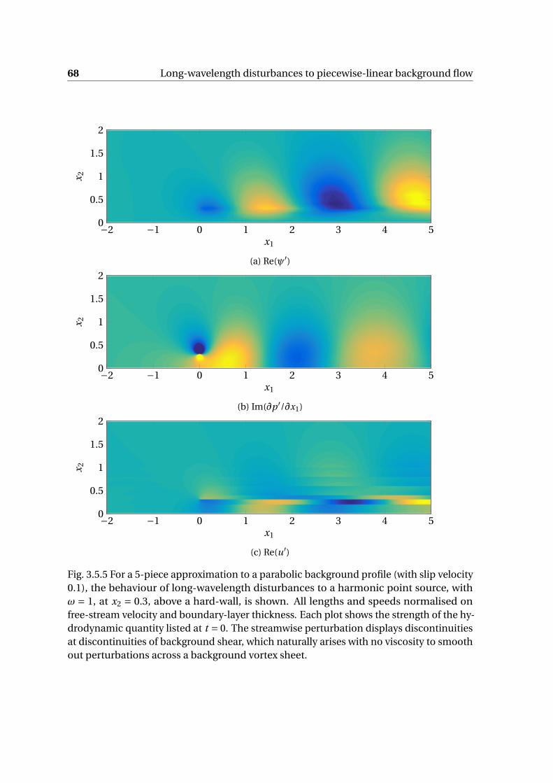
68 Long-wavelength disturbances to piecewise-linear background flow

−2 −1 0 1 2 3 4 50

0.5

1

1.5

2

x1

x 2

(a) Re(ψ′)

−2 −1 0 1 2 3 4 50

0.5

1

1.5

2

x1

x 2

(b) Im(∂p ′/∂x1)

−2 −1 0 1 2 3 4 50

0.5

1

1.5

2

x1

x 2

(c) Re(u′)

Fig. 3.5.5 For a 5-piece approximation to a parabolic background profile (with slip velocity0.1), the behaviour of long-wavelength disturbances to a harmonic point source, withω = 1, at x2 = 0.3, above a hard-wall, is shown. All lengths and speeds normalised onfree-stream velocity and boundary-layer thickness. Each plot shows the strength of the hy-drodynamic quantity listed at t = 0. The streamwise perturbation displays discontinuitiesat discontinuities of background shear, which naturally arises with no viscosity to smoothout perturbations across a background vortex sheet.

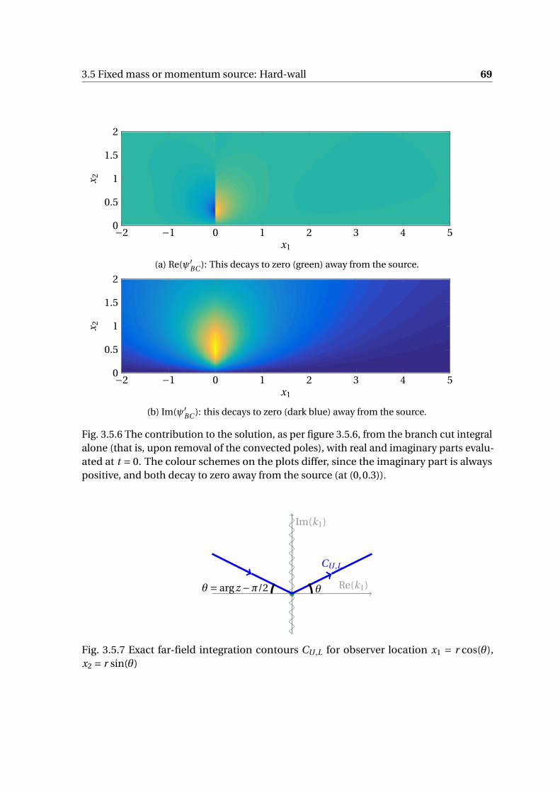
3.5 Fixed mass or momentum source: Hard-wall 69

−2 −1 0 1 2 3 4 50

0.5

1

1.5

2

x1

x 2

(a) Re(ψ′BC ): This decays to zero (green) away from the source.

−2 −1 0 1 2 3 4 50

0.5

1

1.5

2

x1

x 2

(b) Im(ψ′BC ): this decays to zero (dark blue) away from the source.

Fig. 3.5.6 The contribution to the solution, as per figure 3.5.6, from the branch cut integralalone (that is, upon removal of the convected poles), with real and imaginary parts evalu-ated at t = 0. The colour schemes on the plots differ, since the imaginary part is alwayspositive, and both decay to zero away from the source (at (0,0.3)).

Re(k1)

Im(k1)

CU ,L

θθ = arg z −π/2

Fig. 3.5.7 Exact far-field integration contours CU ,L for observer location x1 = r cos(θ),x2 = r sin(θ)

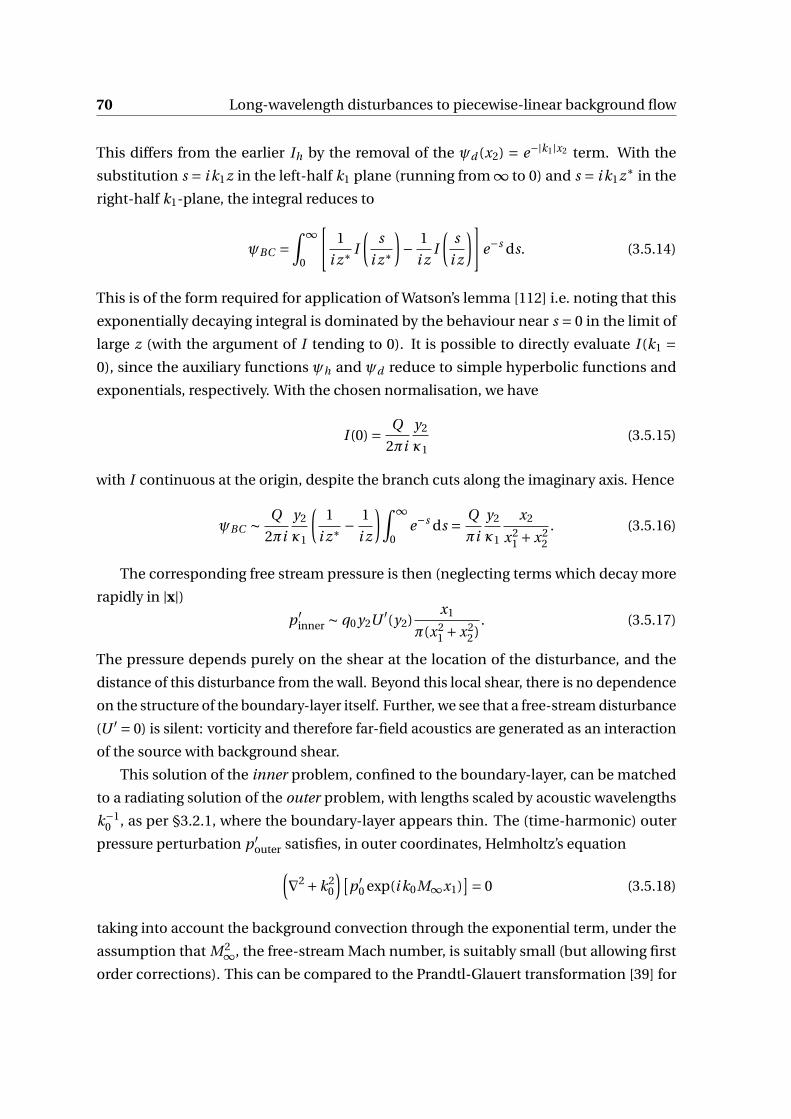
70 Long-wavelength disturbances to piecewise-linear background flow

This differs from the earlier Ih by the removal of the ψd (x2) = e−|k1|x2 term. With the

substitution s = i k1z in the left-half k1 plane (running from ∞ to 0) and s = i k1z∗ in the

right-half k1-plane, the integral reduces to

ψBC =∫ ∞

0

[1

i z∗ I

(s

i z∗

)− 1

i zI

(s

i z

)]e−s ds. (3.5.14)

This is of the form required for application of Watson’s lemma [112] i.e. noting that this

exponentially decaying integral is dominated by the behaviour near s = 0 in the limit of

large z (with the argument of I tending to 0). It is possible to directly evaluate I (k1 =0), since the auxiliary functions ψh and ψd reduce to simple hyperbolic functions and

exponentials, respectively. With the chosen normalisation, we have

I (0) = Q

2πi

y2

κ1(3.5.15)

with I continuous at the origin, despite the branch cuts along the imaginary axis. Hence

ψBC ∼ Q

2πi

y2

κ1

(1

i z∗ − 1

i z

)∫ ∞

0e−s ds = Q

πi

y2

κ1

x2

x21 +x2

2

. (3.5.16)

The corresponding free stream pressure is then (neglecting terms which decay more

rapidly in |x|)p ′

inner ∼ q0 y2U ′(y2)x1

π(x21 +x2

2). (3.5.17)

The pressure depends purely on the shear at the location of the disturbance, and the

distance of this disturbance from the wall. Beyond this local shear, there is no dependence

on the structure of the boundary-layer itself. Further, we see that a free-stream disturbance

(U ′ = 0) is silent: vorticity and therefore far-field acoustics are generated as an interaction

of the source with background shear.

This solution of the inner problem, confined to the boundary-layer, can be matched

to a radiating solution of the outer problem, with lengths scaled by acoustic wavelengths

k−10 , as per §3.2.1, where the boundary-layer appears thin. The (time-harmonic) outer

pressure perturbation p ′outer satisfies, in outer coordinates, Helmholtz’s equation(

∇2 +k20

)[p ′

0 exp(i k0M∞x1)]= 0 (3.5.18)

taking into account the background convection through the exponential term, under the

assumption that M 2∞, the free-stream Mach number, is suitably small (but allowing first

order corrections). This can be compared to the Prandtl-Glauert transformation [39] for

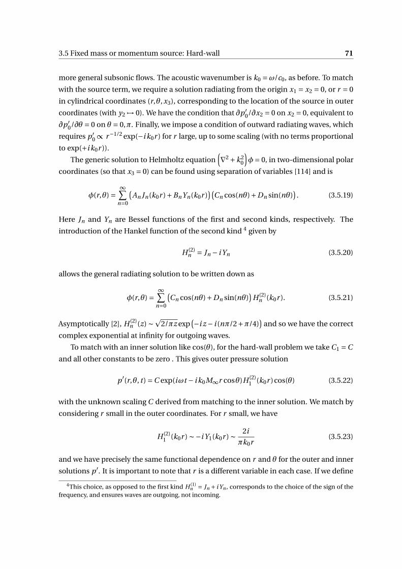
3.5 Fixed mass or momentum source: Hard-wall 71

more general subsonic flows. The acoustic wavenumber is k0 =ω/c0, as before. To match

with the source term, we require a solution radiating from the origin x1 = x2 = 0, or r = 0

in cylindrical coordinates (r,θ, x3), corresponding to the location of the source in outer

coordinates (with y2 7→ 0). We have the condition that ∂p ′0/∂x2 = 0 on x2 = 0, equivalent to

∂p ′0/∂θ = 0 on θ = 0,π. Finally, we impose a condition of outward radiating waves, which

requires p ′0 ∝ r−1/2 exp(−i k0r ) for r large, up to some scaling (with no terms proportional

to exp(+i k0r )).

The generic solution to Helmholtz equation(∇2 +k2

0

)φ= 0, in two-dimensional polar

coordinates (so that x3 = 0) can be found using separation of variables [114] and is

φ(r,θ) =∞∑

n=0

(An Jn(k0r )+BnYn(k0r )

)(Cn cos(nθ)+Dn sin(nθ)

). (3.5.19)

Here Jn and Yn are Bessel functions of the first and second kinds, respectively. The

introduction of the Hankel function of the second kind 4 given by

H (2)n = Jn − i Yn (3.5.20)

allows the general radiating solution to be written down as

φ(r,θ) =∞∑

n=0

(Cn cos(nθ)+Dn sin(nθ)

)H (2)

n (k0r ). (3.5.21)

Asymptotically [2], H (2)n (z) ∼p

2/πz exp(−i z − i (nπ/2+π/4)

)and so we have the correct

complex exponential at infinity for outgoing waves.

To match with an inner solution like cos(θ), for the hard-wall problem we take C1 =C

and all other constants to be zero . This gives outer pressure solution

p ′(r,θ, t ) =C exp(iωt − i k0M∞r cosθ)H (2)1 (k0r )cos(θ) (3.5.22)

with the unknown scaling C derived from matching to the inner solution. We match by

considering r small in the outer coordinates. For r small, we have

H (2)1 (k0r ) ∼−i Y1(k0r ) ∼ 2i

πk0r(3.5.23)

and we have precisely the same functional dependence on r and θ for the outer and inner

solutions p ′. It is important to note that r is a different variable in each case. If we define

4This choice, as opposed to the first kind H (1)n = Jn + i Yn , corresponds to the choice of the sign of the

frequency, and ensures waves are outgoing, not incoming.

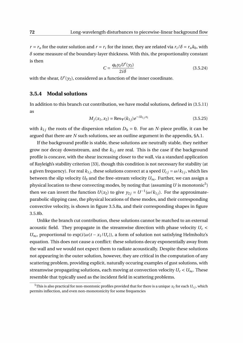
72 Long-wavelength disturbances to piecewise-linear background flow

r = ro for the outer solution and r = ri for the inner, they are related via ri /δ= rok0, with

δ some measure of the boundary-layer thickness. With this, the proportionality constant

is then

C = q0 y2U ′(y2)

2iδ(3.5.24)

with the shear, U ′(y2), considered as a function of the inner coordinate.

3.5.4 Modal solutions

In addition to this branch cut contribution, we have modal solutions, defined in (3.5.11)

as

M j (x1, x2) = ResΨ(k1 j )e−i k1 j x1 (3.5.25)

with k1 j the roots of the dispersion relation Dh = 0. For an N -piece profile, it can be

argued that there are N such solutions, see an outline argument in the appendix, §A.1.

If the background profile is stable, these solutions are neutrally stable, they neither

grow nor decay downstream, and the k1 j are real. This is the case if the background

profile is concave, with the shear increasing closer to the wall, via a standard application

of Rayleigh’s stability criterion [33], though this condition is not necessary for stability (at

a given frequency). For real k1 j , these solutions convect at a speed Uc j =ω/k1 j , which lies

between the slip velocity U0 and the free-stream velocity U∞. Further, we can assign a

physical location to these convecting modes, by noting that (assuming U is monotonic5)

then we can invert the function U (x2) to give y2 j = U−1(ω/k1 j ). For the approximate-

parabolic slipping case, the physical locations of these modes, and their corresponding

convective velocity, is shown in figure 3.5.8a, and their corresponding shapes in figure

3.5.8b.

Unlike the branch cut contribution, these solutions cannot be matched to an external

acoustic field. They propagate in the streamwise direction with phase velocity Uc <U∞, proportional to exp(i (ω(t − x1/Uc )), a form of solution not satisfying Helmholtz’s

equation. This does not cause a conflict: these solutions decay exponentially away from

the wall and we would not expect them to radiate acoustically. Despite these solutions

not appearing in the outer solution, however, they are critical in the computation of any

scattering problem, providing explicit, naturally occuring examples of gust solutions, with

streamwise propagating solutions, each moving at convection velocity Uc <U∞. These

resemble that typically used as the incident field in scattering problems.

5This is also practical for non-montonic profiles provided that for there is a unique x2 for each Uc j , whichpermits inflection, and even non-monotonicity for some frequencies

3.5 Fixed mass or momentum source: Hard-wall 73

U (x2)0.1 0.2 0.3 0.4 0.5 0.6 0.7 0.8 0.9 1

x2

0.2

0.4

0.6

0.8

1

0

(a) The physical location of zeros (o) and poles (x) of the hard-wall dispersion relation Dh(k1,ω)obtained as y2 =U−1(ω/k1). As can be seen, each linear piece supports a mode (when the profileis monotonic).

0 0.2 0.4 0.6 0.8 1 1.2 1.4 1.6 1.8 20

0.2

0.4

0.6

0.8

1

x2

pd

(x2;z

)

(b) The corresponding mode shapes. Here, the perturbation pressure shape is plotted throughoutthe boundary layer, normalised to be 1 at the maximum. The peaks of the modes roughly corre-spond to the velocity of the modes, as per the previous plot. Modes with physical location muchcloser to the boundary-layer thickness (δ= 1) have an impact further beyond the boundary-layer.Further, pressure is broadly constant between the physical mode location and the wall (on which∂p ′/∂x2 = 0).

Fig. 3.5.8 For the parabolic profile (II), approximated by a 5-piece linear profile, thephysical locations within the boundary-layer, and shapes of the 5 convected modes areshown for ω= 1.

74 Long-wavelength disturbances to piecewise-linear background flow

3.5.5 Variation of internal shear

Consider the two-piece profile, case I, with slip velocity U0 allowed to vary but otherwise

the profile is held fixed. This leads to a thin region of variable background shear for

x2 ∈ (0,δ1 = 0.2), with a broad region of low shear outside this region. This is an ideal

setup to investigate the effect of shear shielding, whereby an internal shear layer may

reduce wall pressure or scattered noise, or alternatively a thin region of shear may be

a large source of noise. A mass source only generates vortical disturbances when the

background shear is non-zero, and hence inclusion of a mass source in the outer region

(x2 ∈ (δ1,δ2 = 1)) provides a consistent generator of vorticity (with the shear constant in

this region, independent of U0).

Indeed, it can be seen that the far-field acoustic response to a mass source is un-

changed, with the acoustic response a function of the local background shear and source

location (and strength) only, as per (3.5.24). This might suggest that varying internal shear

has little effect on the trailing vorticity and excited convected modes. This is not the case,

however, as demonstrated in figure 3.5.9. The case with U0 = 0.75 is treated as a base

case, this corresponding to the internal shear σ0 = (U1 −U0)/(δ1) being the same as the

external shear, σ1 = (U∞−U1)/(δ∞−δ1), i.e. an essentially a single-piece profile. As the

internal shear is increased, a shorter-wavelength mode becomes visible, gradually increas-

ing in strength. This mode has the shortest wavelength (and is strongest) in the non-slip

case U0 = 0 (figure 3.5.9d), with the “outer mode” that dominates in the single-piece plot

(figure 3.5.9a) essentially invisible. Further we note the disturbance at the source itself,

y2 = 0.5, are identical between the plots: the source is not varying in strength.

For the two-piece case we have two convected modes, roots of the dispersion relation

0 = Dh(ω,k1)

= 1+∆1

(1−e−2κδ1

)+∆2

(1−e−2κδ2

)+∆1∆2

(1−e−2κδ2 −e−2κδ1 −e−2κ(δ2−δ1)

) (3.5.26)

when we hold ω fixed. The zeros are real for all ω provided U0 ≤ 0.75, which follows from

Rayleigh’s criterion (the profile is non-inflecting, U0 = 0.75 corresponding to exactly the

case where shear is continuous at x2 = δ1). In this range,there is an "outer" mode with

k(o)1 ∈ (ω/U∞,ω/U1) and an "inner" mode with k(i )

1 ∈ (ω/U1,ω/U0), both of which can be

mapped to a physical location via inversion of k1 =ω/U (x2), which is unambiguous for

a monotonic profile, and remains unambiguous for a slightly inflecting profile, in this

case U0 ∈ (0.75,0.825) (a range which depends on frequency ω). The behaviour of these

modes is shown as U0 is varied (for frequency ω= 1 fixed) in figure 3.5.10, showing the

coalescence of the modes at some critical value of U0 > 0.75. After this point, the modes

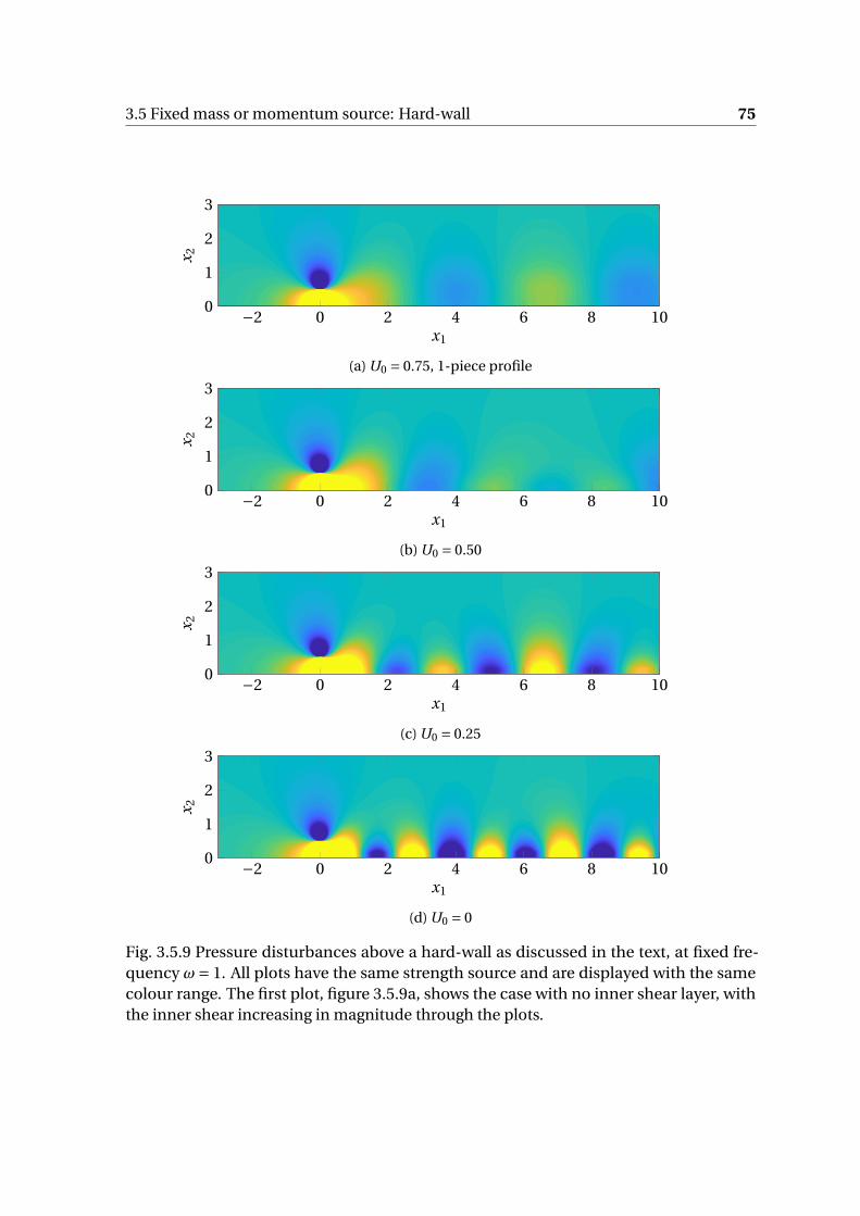
3.5 Fixed mass or momentum source: Hard-wall 75

−2 0 2 4 6 8 100

1

2

3

x1

x 2

(a) U0 = 0.75, 1-piece profile

−2 0 2 4 6 8 100

1

2

3

x1

x 2

(b) U0 = 0.50

−2 0 2 4 6 8 100

1

2

3

x1

x 2

(c) U0 = 0.25

−2 0 2 4 6 8 100

1

2

3

x1

x 2

(d) U0 = 0

Fig. 3.5.9 Pressure disturbances above a hard-wall as discussed in the text, at fixed fre-quency ω= 1. All plots have the same strength source and are displayed with the samecolour range. The first plot, figure 3.5.9a, shows the case with no inner shear layer, withthe inner shear increasing in magnitude through the plots.

76 Long-wavelength disturbances to piecewise-linear background flow

become complex conjugates of each other, and lose stability. U0 = 0.75 corresponds to

a single-piece profile, and we see the location of the inner mode is exactly x2 = 0.2, with

k(i )1 =ω/U1 = 1.2 for U0 = 0.75. Dh has a pole at k1 =ω/U1 for all U0, which cancels out

this zero for U0 = 0.75, resulting in the expected single observed zero of the single-piece

profile.

It is also worth getting a handle on the shape of these modes, as done (again in the

case ω= 1) in figure 3.5.11. The two families of modes have similar shapes, exponentially

decaying beyond the shear layer they correspond to, and remaining broadly constant

across their shear-layer. We note the hard-wall condition translates to ∂p ′/∂x2 = 0, which

clearly holds in all these cases. All the plots are normalised to behave as exp(−|k1|x2)

outside the boundary-layer, which allows noting the gradual increase in strength of the

inner mode with inner shear. The mode decays rapidly across the boundary-layer, for

x2 > δ1 = 0.2. Conversely, the outer mode shape is broadly unchanged with varying inner

shear, being as it is driven by the outer shear layer. In both cases, the peak of the modal

disturbance roughly corresponds to the “physical location” of the disturbance as per

figure 3.5.10b, which lends weight to this earlier designation.

The full inversion plots figure 3.5.9 show that the inner mode gradually dominates as

U0 is decreased (and internal shear increased). We can get a handle on the strength of the

excitation of each mode by revisiting the modal contribution M j from (3.5.11). Without

loss of generality focusing on the wall pressure (which, as the mode shape profiles have

suggested, is broadly the same as the perturbation pressure across each shear layer), we

quantify the strength of modal solutions via

ResPΨ(k1 j ) ∝ pd (0;k1 j )ψh(y2;k1 j )

D ′h(k1 j )

1

k1 j −κ1(3.5.27)

with all other terms dependent only on source location and background shear. For k1 =k(o,i )

1 , φd and φh are proportional to each other, since these modal solutions satisfy both

the hard-wall and decaying boundary conditions. This contribution is plotted, for fixed

values of y2, in figure 3.5.12. Three values of y2 are shown: firstly y2 = 0.5 and y2 = 0.8,

respectively above and below the physical location of the outer mode. Both plots show

the same broad trend: when the inner shear is equal to the outer shear, i.e. U0 = 0.75, only

the outer mode is excited (shown in blue). This is expected as the inner mode does not

exist for this single-piece profile. As U0 decreases, the inner mode is gradually excited

more and more, whilst the excitation of the outer mode reduces. They cross over at some

internal shear, and for high internal shears the inner mode dominates. There are, however,

intermediate ranges of shear in which the total wall pressure is less than it would be if the

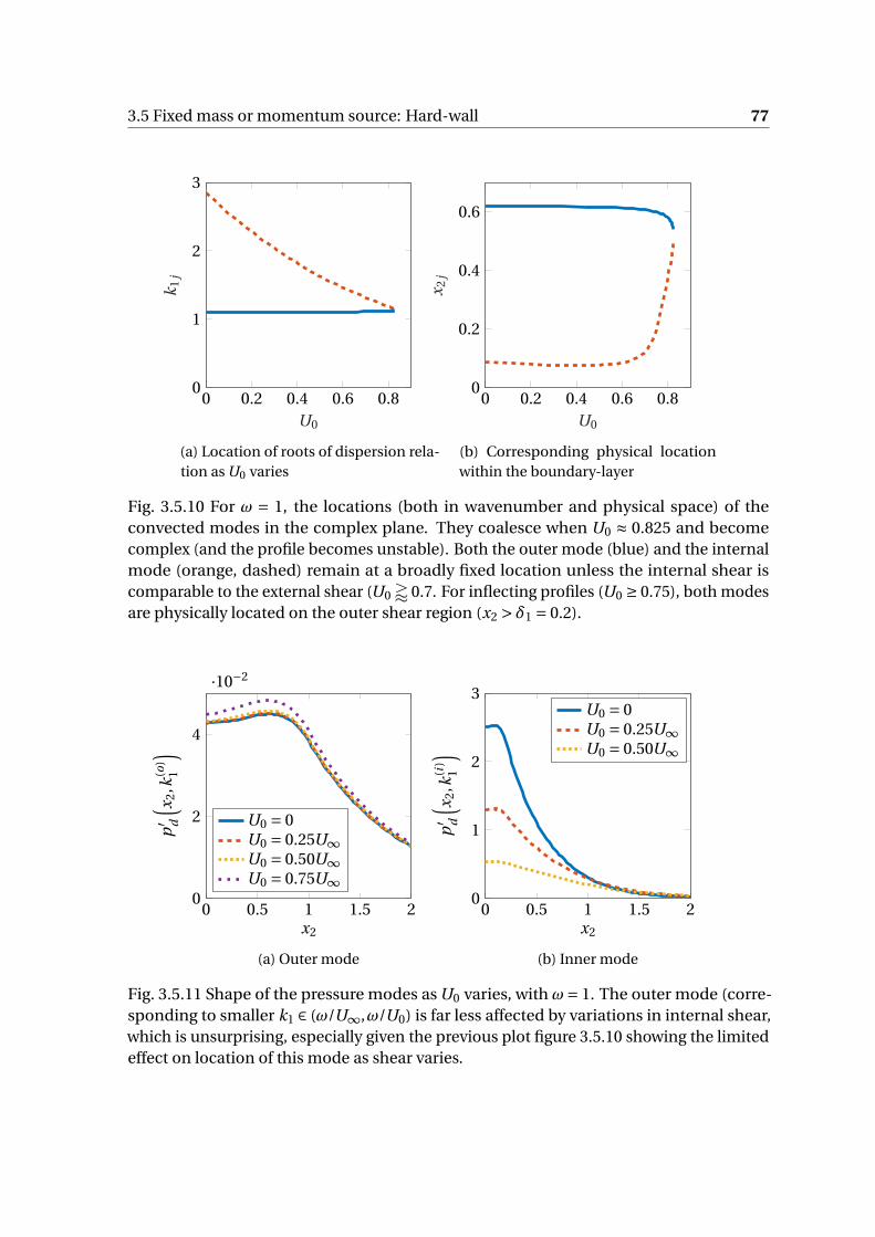
3.5 Fixed mass or momentum source: Hard-wall 77

0 0.2 0.4 0.6 0.80

1

2

3

U0

k1

j

(a) Location of roots of dispersion rela-tion as U0 varies

0 0.2 0.4 0.6 0.80

0.2

0.4

0.6

U0x 2

j(b) Corresponding physical locationwithin the boundary-layer

Fig. 3.5.10 For ω = 1, the locations (both in wavenumber and physical space) of theconvected modes in the complex plane. They coalesce when U0 ≈ 0.825 and becomecomplex (and the profile becomes unstable). Both the outer mode (blue) and the internalmode (orange, dashed) remain at a broadly fixed location unless the internal shear iscomparable to the external shear (U0 ' 0.7. For inflecting profiles (U0 ≥ 0.75), both modesare physically located on the outer shear region (x2 > δ1 = 0.2).

0 0.5 1 1.5 20

2

4

·10−2

x2

p′ d

( x 2,k

(o)

1

)

U0 = 0U0 = 0.25U∞U0 = 0.50U∞U0 = 0.75U∞

(a) Outer mode

0 0.5 1 1.5 20

1

2

3

x2

p′ d

( x 2,k

(i)

1

)

U0 = 0U0 = 0.25U∞U0 = 0.50U∞

(b) Inner mode

Fig. 3.5.11 Shape of the pressure modes as U0 varies, with ω= 1. The outer mode (corre-sponding to smaller k1 ∈ (ω/U∞,ω/U0) is far less affected by variations in internal shear,which is unsurprising, especially given the previous plot figure 3.5.10 showing the limitedeffect on location of this mode as shear varies.

78 Long-wavelength disturbances to piecewise-linear background flow

0 0.2 0.4 0.60

0.05

0.1

0.15

0.2

U0

|PM

j(0,

0)|

y2 = 0.5, outery2 = 0.5, innery2 = 0.8, outery2 = 0.8, inner

(a) y2 = 0.5,0.8

0 0.2 0.4 0.60

50

100

150

200

250

U0|P

Mj(

0,0)|

y2 = 0.61, outery2 = 0.61, inner

(b) y2 = 0.61

Fig. 3.5.12 Wall pressure of modal contributions from a fixed source, as the inner shearis varied (through variation of U0). In all cases, ω = 1. Broadly there is a transfer fromthe outer mode to the inner mode as the shear is increased (U0 decreased) though thesingular case when the outer mode location k(o)

1 passes through κ1 (the forcing location)is shown in figure 3.5.12b, with the outer mode crossing x2 = 0.61 seen in figure 3.5.10b.

internal shear layer were not there, here with U0 ≈ 0.5 and so σ0 ≈ 1.5. Finally, the case

y2 = 0.61 is shown in figure 3.5.12b. This corresponds to k(o)1 ≈ κ1 =ω/U (y2). Whilst k(o)

1

varies only slightly with U0, in this case it passes across κ1, where the mode excitation is

singular. Varying the inner shear moves the excited mode location further from the forcing

location, and thus, in this singular case, greatly reduces noise for all U0 < 0.6, though the

singular nature of this case is worth reemphasising.

We have seen that increasing internal shear can draw energy away from an outer,

large-scale mode, though at the expense of exciting an inner mode. Provided these are

suitably balanced, there is some argument for a shear-shielding effect, that an inner shear

layer can reduce wall-pressure. If this disturbance is incident on some scattering junction,

the resultant far-field noise (driven by wall pressure) could be reduced, though this is a

careful optimisation that depends on the frequency of interest.

3.6 Lined walls: pressure-release and impedance conditions

The numerical method changes little for the pressure-release solution, where we instead

impose p ′ = 0 on x2 = 0. This generalises neatly to considering a more general impedance

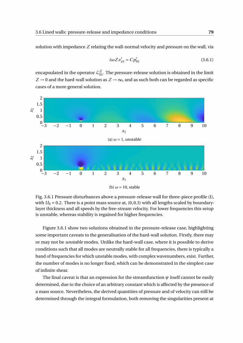
3.6 Lined walls: pressure-release and impedance conditions 79

solution with impedance Z relating the wall-normal velocity and pressure on the wall, via

iωZ v ′o1 =C p ′

01 (3.6.1)

encapsulated in the operator LZ01. The pressure-release solution is obtained in the limit

Z → 0 and the hard-wall solution as Z →∞, and as such both can be regarded as specific

cases of a more general solution.

−3 −2 −1 0 1 2 3 4 5 6 7 8 9 100

0.51

1.52

x1

x 2

(a) ω= 1, unstable

−3 −2 −1 0 1 2 3 4 5 6 7 8 9 100

0.51

1.52

x1

x 2

(b) ω= 10, stable

Fig. 3.6.1 Pressure disturbances above a pressure-release wall for three-piece profile (I),with U0 = 0.2. There is a point mass source at, (0,0.3) with all lengths scaled by boundary-layer thickness and all speeds by the free-stream velocity. For lower frequencies this setupis unstable, whereas stability is regained for higher frequencies.

Figure 3.6.1 show two solutions obtained in the pressure-release case, highlighting

some important caveats to the generalisation of the hard-wall solution. Firstly, there may

or may not be unstable modes. Unlike the hard-wall case, where it is possible to derive

conditions such that all modes are neutrally stable for all frequencies, there is typically a

band of frequencies for which unstable modes, with complex wavenumbers, exist. Further,

the number of modes is no longer fixed, which can be demonstrated in the simplest case

of infinite shear.

The final caveat is that an expression for the streamfunction ψ itself cannot be easily

determined, due to the choice of an arbitrary constant which is affected by the presence of

a mass source. Nevertheless, the derived quantities of pressure and of velocity can still be

determined through the integral formulation, both removing the singularities present at

80 Long-wavelength disturbances to piecewise-linear background flow

k1 = 0. Since these physical quantities, rather than the streamfunction itself, are important

in practice, this does not pose difficulties.

3.6.1 Quantity of pressure-release modes

Typically there appear to be N +1 roots of the pressure-release dispersion function. This

is not always the case, however, particularly in the singular case ω≈σ0, the wall-shear.

Consider first the 1-piece dispersion function for pressure-release boundary condi-

tions (3.4.24), namely

Dp =((1+∆)−∆e−2κδ

)+ κC0

C ′0

((1+∆)+∆e−2κδ

). (3.6.2)

In the limit δ→∞, this reduces simply to

Dp = 1+ κC0

C ′0

= 1− |k1|(ω−U0k1)

k1σ0. (3.6.3)

The number of zeros of this relation, corresponding to convected modes, depends on

the relative magnitude of ω and σ0 (the shear). If ω > σ0, there is a single zero at k1 =U−1

0 (ω−σ0) whereas if ω<−σ0, there is a zero at k1 =U−10 (ω+σ0). In the intermediate

region, −σ0 <ω<σ0, there are no zeros. In a sense there are always two zeros, but one

of them (and possible both) lie on the alternative Riemann sheet, due to the branch cuts

of κ. It is worth noting that all zeros move to infinity in the limit U0 → 0, which causes

difficulties in consideration of the non-slipping case.

The difference in numbers of zeros for ω≷σ does not generalise to a finite boundary-

layer, as shall be seen below (for example figure 3.6.3 which looks at the simplest case of a

single shear layer). Whereas the infinite shear case either has one or no zeros, there are

always at least two zeros in the case of a single shear layer, which might rise to more in

certain situations, in particular when frequency and shear are of comparable size. The dis-

appearance of the shear mode is, however, an artefact of the infinite shear approximation.

A stability analysis is done for the 5-piece profile (profile II) in the next section, and 6

zeros are found with pressure-release boundary conditions (for ωδ/U∞ = 1). This seems

completely expected, based on the hard-wall case (where an N -piece profile has N zeros),

with the extra zero arising from the zero that exists in the uniform flow case (due to the

slightly more complicated boundary operator). This is not, however, necessarily the case.

If we return to the 1-piece dispersion relation, and scale all lengths and speeds by δ and

U∞ respectively (so that the shear is (1−U0)), then Dp as a function of k1 has only two

3.6 Lined walls: pressure-release and impedance conditions 81

parameters, ω and U0, explicitly

Dp (k1;ω,U0) =(

1− sgn(k1)(ω−U0k1)

1−U0

)(1+ (1−U0)sgn(k1)

2(ω−k1)

)

−(

1+ sgn(k1)(ω−U0k1)

1−U0

)(1−U0)sgn(k1)

2(ω−k1)e−2|k1|. (3.6.4)

We focus on the right-half plane, with Re(k1) > 0 (so that sgn(k1) = k1/|k1| = 1), and

assume U0 > 0. This function is plotted in figure 3.6.2, for the non-slipping case U0 = 0,

with frequency ω = 1.1. We saw in the infinite shear case that ω ≷ 1 gives rise to two

different behaviours, and by including a finite boundary-layer we are in a position to

investigate this. For ω≈ 1, as in the figure, more zeros are apparent. In the limit ω−1 ≡ϵ≪ 1 we have approximate dispersion relation (in the RHk1P)

Dp ≈−ϵ(1+ 1

2(1−k1)

)−e−2k1 (1−k1). (3.6.5)

The reduced dispersion relation Dp = (1−k1)Dp then has zeros satisfying

e−2k1 +ϵ(

3

2−k1

)= 0 (3.6.6)

which permits exact solutions in terms of the Lambert-W function (or product log func-

tion), namely

k1 ≈ 3

2+ 1

2Wn

(2

ϵe3

)(3.6.7)

with Wn the inverse of z = WneWn , choosing the nth branch. This function is available

in most common programming languages, and thus this approximation can easily be

checked. Based on the earlier assumption, only the solutions with Re(k1) > 0 are valid as

zeros of the exact dispersion relation, and thus the number of zeros varies as ϵ decreases.

We can get a bound for the number of zeros with positive real part by looking at the

asymptotic behaviour of Wn as n is increased. Following Corless et al. [29], for n large we

have

Wn(z) ≈ log(z)+2πi n − log(log(z)+2πi n) (3.6.8)

which means the approximate location of the zeros, for n large, are

k1 ≈ 1

2

(log(2/ϵ)+2πi n − log

[log(2/ϵ)−3+2πi n

]). (3.6.9)

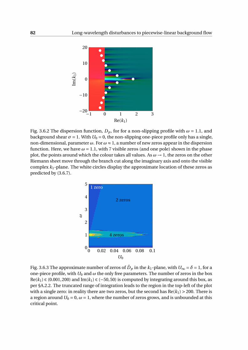
82 Long-wavelength disturbances to piecewise-linear background flow

−1 0 1 2 3−20

−10

0

10

20

Re(k1)

Im(k

1)

Fig. 3.6.2 The dispersion function, Dp , for for a non-slipping profile with ω = 1.1, andbackground shear σ= 1. With U0 = 0, the non-slipping one-piece profile only has a single,non-dimensional, parameterω. Forω≈ 1, a number of new zeros appear in the dispersionfunction. Here, we have ω= 1.1, with 7 visible zeros (and one pole) shown in the phaseplot, the points around which the colour takes all values. As ω→ 1, the zeros on the otherRiemann sheet move through the branch cut along the imaginary axis and onto the visiblecomplex k1-plane. The white circles display the approximate location of these zeros aspredicted by (3.6.7).

2 zeros

4 zeros

1 zero

0 0.02 0.04 0.06 0.08 0.10

1

2

3

4

5

U0

ω

Fig. 3.6.3 The approximate number of zeros of Dp in the k1-plane, with U∞ = δ= 1, for aone-piece profile, with U0 and ω the only free parameters. The number of zeros in the boxRe(k1) ∈ (0.001,200) and Im(k1) ∈ (−50,50) is computed by integrating around this box, asper §A.2.2. The truncated range of integration leads to the region in the top-left of the plotwith a single zero: in reality there are two zeros, but the second has Re(k1) > 200. There isa region around U0 = 0, ω= 1, where the number of zeros grows, and is unbounded at thiscritical point.

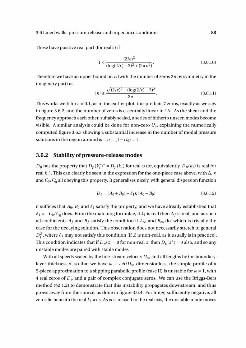
3.6 Lined walls: pressure-release and impedance conditions 83

These have positive real part (for real ϵ) if

1 < (2/ϵ)2

(log(2/ϵ)−3)2 + (2πn2). (3.6.10)

Therefore we have an upper bound on n (with the number of zeros 2n by symmetry in the

imaginary part) as

|n| ≤√

(2/ϵ)2 − (log(2/ϵ)−3)2

2π. (3.6.11)

This works well: for ϵ= 0.1, as in the earlier plot, this predicts 7 zeros, exactly as we saw

in figure 3.6.2, and the number of zeros is essentially linear in 1/ϵ. As the shear and the

frequency approach each other, suitably scaled, a series of hitherto unseen modes become

visible. A similar analysis could be done for non-zero U0, explaining the numerically

computed figure 3.6.3 showing a substantial increase in the number of modal pressure

solutions in the region around ω=σ= (1−U0) = 1.

3.6.2 Stability of pressure-release modes

Dp has the property that Dp (k∗1 )∗ = Dp (k1) for real ω (or, equivalently, Dp (k1) is real for

real k1). This can clearly be seen in the expression for the one-piece case above, with ∆, κ

and C0/C ′0 all obeying this property. It generalises nicely, with general dispersion function

Dℓ = (A0 +B0)−ℓ1κ(A0 −B0) (3.6.12)

it suffices that A0, B0 and ℓ1 satisfy the property, and we have already established that

ℓ1 =−C0/C ′0 does. From the matching formulae, if k1 is real then ∆ j is real, and as such

all coefficients A j and B j satisfy the condition if A∞ and B∞ do, which is trivially the

case for the decaying solution. This observation does not necessarily stretch to general

D Zℓ

, where ℓ1 may not satisfy this condition (if Z is non-real, as it usually is in practice).

This condition indicates that if Dp (z) = 0 for non-real z, then Dp (z∗) = 0 also, and so any

unstable modes are paired with stable modes.

With all speeds scaled by the free-stream velocity U∞ and all lengths by the boundary-

layer thickness δ, so that we have ω→ ωδ/U∞ dimensionless, the simple profile of a

5-piece approximation to a slipping parabolic profile (case II) is unstable for ω= 1, with

4 real zeros of Dp and a pair of complex conjugate zeros. We can use the Briggs-Bers

method (§2.1.2) to demonstrate that this instability propagates downstream, and thus

grows away from the source, as done in figure 3.6.4. For Im(ω) sufficiently negative, all

zeros lie beneath the real k1 axis. As ω is relaxed to the real axis, the unstable mode moves

84 Long-wavelength disturbances to piecewise-linear background flow

across the real axis, and is thus convectively unstable. However, it poses no problems in

deformation of the Fourier inversion contour from the real axis, to account for this mode

being in some generalised lower half k1 plane. That this mode propagates downstream is

unsurprising: the real part of the wavenumber lies on the critical-layer, corresponding to

solutions convected with the mean flow, and naturally we would expect this solution to be

convected downstream with the (positive) mean flow. Where the mean flow is negative

(for example if moving in the frame with a convected source, with negative background

velocity between the source and the wall), it is very possible that upstream propagating

disturbances might exist and Briggs-Bers should be used carefully.

This analysis can be performed using the zero-finding methods outlined in the ap-

pendix, §A.2.2. Iterating over some array of frequencies, ω j , a guess for the location of

zeros for case ω j+1 is provided by the computed location for ω j . Provided ω j+1 −ω j is

sufficiently small, the displacement in the location of the root is small enough that the

previous location is a good estimate for the new location, and thus Newton-Raphson

efficiently determines the location of the new zero. The most difficult case is the initial

case, where all zeros must be located with no information. For the plot in figure 3.6.4, the

case of real ω was computed first, and then the imaginary part was gradually made more

negative.

We have previously noted that the same background flow might be unstable at some

frequencies and yet stable at other frequencies. As the magnitude of the frequency changes,

the movement of modes can be observed. At some critical frequency, two (neutrally

stable) zeros in the k1-plane will meet, and with further variation in frequency become a

complex conjugate pair. The alternative process may happen at some higher frequency

still, with the two conjugate modes coming together and restabilising. Numerically, this

proceeds analogously to the above, with instead of small variation of Im(ω), Re(ω) is varied

instead, with zeros found using a Newton-Raphson method with initial guess given by

the preceding solution. This is demonstrated for the simple two-piece case in figure 3.6.5,

with the two modes unstable for lower frequencies stabilising at higher frequencies. As a

caveat to the numerical procedure outlined above: there is a critical frequency at which

two modes are coincident (corresponding to the boundary of stability). After this point,

the preceding value of mode location has two identical values, and thus this routine fails

to find the final mode. To get around this, figure 3.6.5 was computed in both directions

(from ω= 0.5 and from ω= 8) and matched in the middle.

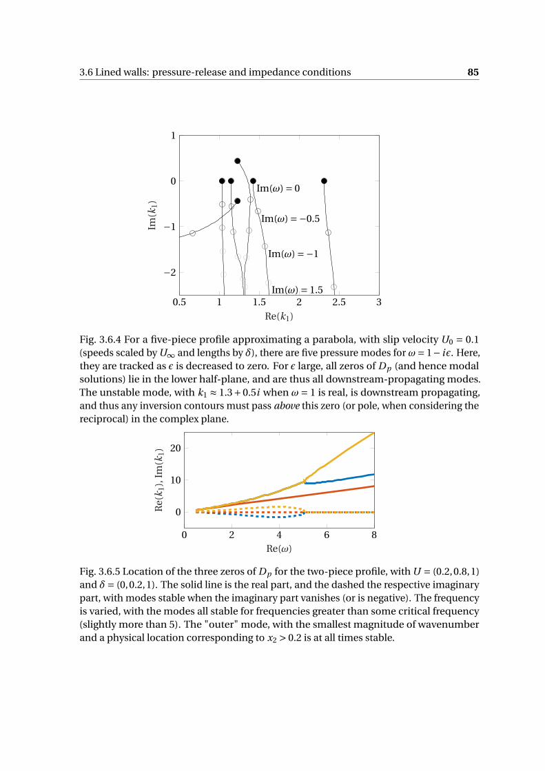
3.6 Lined walls: pressure-release and impedance conditions 85

0.5 1 1.5 2 2.5 3

−2

−1

0

1

Im(ω) = 0

Im(ω) =−0.5

Im(ω) =−1

Im(ω) = 1.5

Re(k1)

Im(k

1)

Fig. 3.6.4 For a five-piece profile approximating a parabola, with slip velocity U0 = 0.1(speeds scaled by U∞ and lengths by δ), there are five pressure modes for ω= 1− iϵ. Here,they are tracked as ϵ is decreased to zero. For ϵ large, all zeros of Dp (and hence modalsolutions) lie in the lower half-plane, and are thus all downstream-propagating modes.The unstable mode, with k1 ≈ 1.3+0.5i when ω= 1 is real, is downstream propagating,and thus any inversion contours must pass above this zero (or pole, when considering thereciprocal) in the complex plane.

0 2 4 6 8

0

10

20

Re(ω)

Re(

k1),

Im(k

1)

Fig. 3.6.5 Location of the three zeros of Dp for the two-piece profile, with U = (0.2,0.8,1)and δ= (0,0.2,1). The solid line is the real part, and the dashed the respective imaginarypart, with modes stable when the imaginary part vanishes (or is negative). The frequencyis varied, with the modes all stable for frequencies greater than some critical frequency(slightly more than 5). The "outer" mode, with the smallest magnitude of wavenumberand a physical location corresponding to x2 > 0.2 is at all times stable.

86 Long-wavelength disturbances to piecewise-linear background flow

3.6.3 Impedance modes

Having separately analysed the case of a wall with no penetration of the fluid through

it, and of a wall which cannot support any pressure, we now consider the case where

the perturbation pressure and velocity are linked by some linear relationship, quantified

in this case by an impedance Z , with boundary conditions as posed in table 3.1. The

introduction of this Z does little to change the behaviour of the method of solution,

with decomposition into branch cut contributions (and thus far-field noise) and finding

propagating modal solutions combining to give a complete solution.

The biggest change from the pressure-release case is that, unless Z is purely imaginary,

the dispersion relationship DZ no longer satisfies the symmetry property DZ (k∗1 ) = D∗

Z (k1),

or equivalently that the relationship is real for real k1. Therefore the resulting modes do

not pair themselves up into complex conjugate pairs, and further none of them are exactly

neutrally stable (all lie off the real axis).

When locating zeros, the first step is typically to eliminate poles of the dispersion

function, which are mostly analytically known (arising directly from the singularities

in the matching formulae for the piecewise linear case, and thus at k1 = ω/U j ). In the

hard-wall case, a reduced dispersion function was defined by multiplying the dispersion

function Dh by the product R(k1,ω) = ∏Nj=1(k1 −ω/U j ), resulting in a function without

poles in the k1-plane, with the only singularities being the branch point at zero and thus

the resulting branch cuts dividing the k1-plane into right and left halves. This reduction

allowed the use of numerical schemes to find zeros of Dh . A similar reduction can be used

in the impedance case. However, an extra pole arises from the definition of ℓZ1 , namely

the pole arising when the denominator of ℓZ1 vanishes, at the roots of

iωZ k21Z p −σ0k1Z p (ω−U0k1) = 0. (3.6.13)

The shear at the wall, σ0, and the flow speed at the wall, U0, both appear as parameters.

The trivial root at k1Z p = 0 can be ignored (though as we have seen, this does affect the

inversion, with care needed at 0), and thus we have an additional pole at

k1Z p = σ0ω

σ0U0 + iωZ= ω/U0

1+ iωZ /(U0σ0). (3.6.14)

The reduced impedance dispersion function is then

DZ (k1;ω) = R(k1;ω)(k1 −k1Z p (ω))Dz(k1;ω). (3.6.15)

3.6 Lined walls: pressure-release and impedance conditions 87

This is now analytic in both the right and left-half planes away from the branch point at

k1 = 0, and thus amenable to numerical zero-finding methods. This additional pole gives

rise to the possibility of an additional zero, giving an estimate of N +2 zeros, for a generic

case (away from the singular behaviour seen if ω∼σ in the pressure-release case): the N

zeros for the pole from each shear layer, the additional one from the pole at k1 = 0 (seen

in the pressure-release case similarly) and the new zero corresponding to this new pole,

k1Z p . The dynamics of the resulting modes, as Z changes, are interesting: when Z = 0 one

of the modes lies at ω/U0 and is exactly cancels the additional pole computed above, so

doesn’t appear for vanishing Z , and thus we reduce to the number of poles seen in the

pressure-release case. Conversely, as |Z | gets large we would expect a reduction to exactly

N modes, and thus two of the zeros must disappear. The only mathematically consistent

ways of this occurring is for them to go through the branch cuts, and thus off the visible

k1-plane, though their contribution might still be seen through the branch-cut integrals;

or for them to go to infinity.

−2 0 2 4 6

−2

−1

0

1

2

|Z | = 0

|Z | =0.916

|Z | =2.57

Re(k1)

Im(k

1)

(a) Z = |Z |e−iπ/4

−2 0 2 4 6

−2

−1

0

1

2

|Z | = 0

Re(k1)

Im(k

1)

(b) Z = |Z |e+iπ/4

Fig. 3.6.6 For simple two-piece profile (U = (0.2,0.8,1); δ = (0,0.2,1), ω = 1), the 4boundary-layer modes are tracked as the amplitude of the impedance is varied, withZ = 0 indicated for all modes.

The boundary-layer modes of a simple two-piece profile are considered in figure 3.6.6,

as the magnitude of Z varies (with complex argument ±π/4). The pressure-release case is

attained at Z = 0. The "outer" mode k1 ∼ 1.11 varies little in Z , and is therefore hard to

pick out on this figure. In both cases the hard-wall modes are found as Z →∞, though

they do not correspond to the same pressure-release modes: in the case Im(Z ) < 0, two

modes (the unstable pressure modes) move behind the branch cut at some finite |Z | and

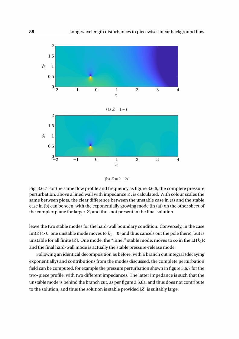
88 Long-wavelength disturbances to piecewise-linear background flow

−2 −1 0 1 2 3 40

0.5

1

1.5

2

x1

x 2

(a) Z = 1− i

−2 −1 0 1 2 3 40

0.5

1

1.5

2

x1

x 2

(b) Z = 2−2i

Fig. 3.6.7 For the same flow profile and frequency as figure 3.6.6, the complete pressureperturbation, above a lined wall with impedance Z , is calculated. With colour scales thesame between plots, the clear difference between the unstable case in (a) and the stablecase in (b) can be seen, with the exponentially growing mode (in (a)) on the other sheet ofthe complex plane for larger Z , and thus not present in the final solution.

leave the two stable modes for the hard-wall boundary condition. Conversely, in the case

Im(Z ) > 0, one unstable mode moves to k1 = 0 (and thus cancels out the pole there), but is

unstable for all finite |Z |. One mode, the “inner” stable mode, moves to ∞ in the LHk1P,

and the final hard-wall mode is actually the stable pressure-release mode.

Following an identical decomposition as before, with a branch cut integral (decaying

exponentially) and contributions from the modes discussed, the complete perturbation

field can be computed, for example the pressure perturbation shown in figure 3.6.7 for the

two-piece profile, with two different impedances. The latter impedance is such that the

unstable mode is behind the branch cut, as per figure 3.6.6a, and thus does not contribute

to the solution, and thus the solution is stable provided |Z | is suitably large.

3.6 Lined walls: pressure-release and impedance conditions 89

3.6.4 Far-field noise

When computing the far-field noise due to a mass source above a hard boundary, we could

directly write down an expression for far-field streamfunction, ψ. However, as we have

seen, the integral expression for the Fourier inversion for ψ has a pole at 0, which causes

difficulties. We can, however, compute expressions for the far-field velocity components

due to the inner solution, which can in turn be matched to an outer solution.

We work with the generic boundary condition, on x2 = 0, with Lψ= ℓ1ψ′+ℓ2ψ= 0.

We have the integral expression for v ′0, the wall-normal velocity perturbation, outiside the

boundary layer (so x2 > δ)

v ′ = Q(y2)

2πi

∫F1

i k1φℓ(y2;k1)

Dℓ(k1)

e−|k1|x2−i k1x1

k1 −κ1dk1 (3.6.16)

with Q defined as for (3.5.6). By Watson’s lemma, this is dominated near k1 = 0, where we

need evaluate both φℓ and Dℓ =Lφd . In this limit the shear jump becomes unimportant,

and we thus have

φℓ ∼ A0e |k1|x2 +B0e−|k1|x2 (3.6.17)

as k1 → 0, (for all x2) where

A0 =− ℓ2

2|k1|+ ℓ1

2(3.6.18a)

B0 =+ ℓ2

2|k1|+ ℓ1

2(3.6.18b)

and Dℓ→−|k1|ℓ1 +ℓ2 as k1 → 0. Both of these results are completely generic, regardless

of the exact form of the boundary condition imposed. If we consider some region of the

complex k1-plane near the origin, we then have

v ′ ∼− Q

2πiκ1

∫F1ϵ

i k1(ℓ1 −ℓ2 y2)

ℓ2 −|k1|ℓ1e−|k1|x2−i k1x1 dk1 (3.6.19)

where we have reduced the exponentials in the auxiliary function for small k1. Introducing

complex observer location z = x1 + i x2, we integrate along the rays parameterised by

s = i k1z∗ for Re(k1) > 0 and s = i k1z for Re(k1) < 0, exactly as in figure 3.5.7. We then have

v ′ ∼− Q

2πiκ1

∫ ∞

0I

(s

i z∗

)e−s ds

i z∗ + Q

2πiκ1

∫ ∞

0I

(s

i z

)e−s ds

i z(3.6.20)

90 Long-wavelength disturbances to piecewise-linear background flow

with

I (k1) = i k1(ℓ1 −ℓ2 y2)

ℓ2 −|k1|ℓ1(3.6.21)

For both the pressure and impedance boundary conditions, we have ℓ2 = 1 and ℓ1 ∼C

C ′ ∼ω

k1σas k1 → 0. It is this singularity of ℓ1 at k1 = 0 that leads to the resulting singularity

of the integrand when computing ψ, for example. With this, we have

I = i k1α

1−αsgn(k1)(3.6.22)

for k1 small, where α=ω/σ is the ratio between the frequency and the background shear

at the wall. Importantly, this is finite (albeit discontinuous) at k1 = 0, for α = ±1. The

far-field contribution is then

v ′ ∼ Q

2πκ1

[α

α−1

1

z∗ − α

α+1

1

z

](3.6.23)

for x2 ≫ δ. We focus firstly on the latter term, noting that 1/z corresponds could cor-

respond to an irrotational velocity potential W = φ+ iψ = log(z). This in turn can be

matched to an irrotational far-field flow φ∝ H (2)0 (k0r ), which is an expected solution of

Helmholtz equation, and critically it does not depend on the angle with respect to the

source, θ. It is exactly the solution due to a mass source in shear flow with no boundary,

and the alternate term, containing 1/z∗, is exactly the image source required to satisfy the

boundary condition on x2 = 0: again radiating like H (2)0 (k0r ). We thus suppose we have a

far-field acoustic potential φ, so that u =∇φ and p ′ = ρ0 Dφ/Dt . φ satisfies the convected

Helmholtz equation, and as such we have (assuming limited angular dependence due to

the form of the inner solution)

φ= e−i k0M∞r cos(θ) AH (2)0 (k0r ) (3.6.24)

which satisfies the convected Helmholtz equation (for U∞ ≪ 1), as noted in §3.5.3 and

equation (3.5.18). As r → 0,

H (2)0 (k0r ) ∼ 2i

πlog(k0r /2). (3.6.25)

Matching both terms of the inner solution to this (assuming their contribution is the same,

or for example letting x2 7→ −x2 to properly deal with the z∗ term), we have

2i

πA = Q

2πκ1

[α

α−1− α

α+1

]. (3.6.26)

3.7 Fixed mass or momentum source: Wake 91

and so

A = Q

2iκ1

α

α2 −1(3.6.27)

From this, we can deduce we have an outgoing cylindrical pressure wave, with p approxi-

mately given by iωφ. There are two contributions: the contribution from the source itself,

and the contribution from the reflection off the wall. Since the reflected solution does

not correspond to the original solution, due to the distortion by the boundary-layer shear,

they are not cancelled out exactly and the radiated sound consists of the summation of

two cylindrical waves (in phase through the long-wavelength assumption). Compare this

with the hard-wall, where the choice of boundary conditions ensured a cancellation of

original and image sources, and a dipole in the far-field.

It is worth stress-testing this result, especially due to the non-routine methods of

dealing with the z∗ term. If there is no shear, and no flow, we have α→ 0 and A → 0. This

does not correspond to no far-field noise due to the source, just that the monopole-type

source vanishes. There will still be the dipole source. Essentially, when the flow is uniform,

the original source (above the wall) and the image source (below the wall) exactly cancel

each other out in the far-field. When ω is small, A is non-zero since κ1 as well as α is

proportional to ω.

Finally, we note that this is singular when |α| = 1, and large for |α| ≈ 1. It is worth

comparing this result to the earlier analysis of the single-piece shear, when the limit α→ 1

gave rise to a countable infinity of otherwise unseen modal solutions.

3.7 Fixed mass or momentum source: Wake

As a final boundary condition, we consider the case with no surface at x2 = 0, with instead

the domain stretching to x2 →−∞. Before we insisted on solely outgoing waves as x2 →∞,

leading to the imposition of decay like exp(−|k1|x2) in streamwise Fourier space. This

time, we similarly impose decay as x2 → −∞, and thus behaviour like exp(|k1|x2), as

x2 → −∞, in Fourier space, which motivates the construction of the second auxiliary

function, controlling behaviour beneath the vortex sheet at x2 = y2, as being the solution

that exponentially decays as x2 →−∞.

For concreteness, we consider the flow profile illustrated in figure 3.3.2 (in turn ex-

plaining the extended domain of that figure) and define two auxiliary functions ψ1,2 to

be the solution to the governing equations ((d2/dx22 −k2

1)ψ = 0, with associated jump

92 Long-wavelength disturbances to piecewise-linear background flow

conditions at δ j ) such that

ψ1(x2) = exp(−|k1|x2) x2 > δN+ ≡ δ∞ (3.7.1a)

ψ2(x2) = exp(|k1|x2) x2 < δN− ≡ δ−∞ (3.7.1b)

That is,ψ1 =ψd is the decaying solution from before. If we defined an reversed flow profile

via U−j =U− j and δ−j = δ− j , then ψ2(x2) =ψU−

d (−x2), with the decaying solution arising

from the reversed profile. For a symmetric profile, defined here as one with U j =U− j and

δ j = δ− j , then ψ2(x2) =ψ1(−x2), which somewhat simplifies the analysis.

The general solution to the point mass source is unchanged, under the choice of the

new auxiliary functions, with

ψ01(x2) =− U ′(y2)q0

U (y2)ρ(y2)

1

i (k1 −κ1)

1

W (y2)×

ψ1(x2;k1)ψ2(y2;k1) x2 > y2,

ψ2(x2;k1)ψ1(y2;k1) x2 < y2,(3.7.2)

exactly as in (3.4.15). Whilst the Wronskian, as a function of y2, is easy to define as

W (y2) =ψ′1(y2)ψ2(y2)−ψ′

2(y2)ψ1(y2), (3.7.3)

we would like a y2-independent expression, namely W (0). Since, typically, we have chosen

x2 = 0 to correspond to δ0, care is required here with the values ofψ′1 andψ′

2 discontinuous

over δ0. Further, to really exploit the generalisation of φd to generate φ2, we would like to

evaluate φ2 below the wake, at x2 = 0−. Using the jump condition, we have

W (0+) =ψ′1(0+)ψ2(0−)−ψ′

1(0+)ψ2(0−)+∆0ψ1(0+)ψ2(0−). (3.7.4)

As before, the jump across the shear junction at δ0, this time corresponding to the wake, is

controlled by

∆0 =i k1

(σ(0+)−σ(0−)

)i (ω−U0k1)

. (3.7.5)

We compare this to a dispersion function, created directly from imposition of pressure

and velocity across the wake, as

Dw (ω,k1) =P0+01ψ1V

0−01ψ2 −P0−

01ψ2V0+01ψ1 (3.7.6)

with zeros of this function directly corresponding to solutions of the governing equation

which decay as |x2| →∞ in both directions. As hoped, and analogously with the earlier

3.7 Fixed mass or momentum source: Wake 93

work, this corresponds to the Wronskian with

Dw = i (ω−k1U0)W, (3.7.7)

and we therefore have exactly the solution of the form required. Fourier inversion can then

proceed as before: modal solutions from zeros of the dispersion function are combined

with integration around the |k1| branch cut to determine a complete, causal solution.

3.7.1 Simplification in the symmetric case

As noted above, ψ1 and ψ2 are closely linked when the background profile is symmetric,

withψ1(0+) =ψ2(0−) andψ′1(0+) =−ψ′

2(0−), with the dispersion function in the symmetric

case therefore reducing to

Dw = 2V0+01ψdP

0+01ψd = 2Dh ·Dp , (3.7.8)

with ψd simply the decaying solution as when there was a boundary at x2 = 0 (so corre-

sponding to ψ1).

We have a natural separation into hard-wall and pressure-release solutions, which is

unsurprising, by considering constructing modal solutions. Suppose we have a hard-wall

modal solution ψmh(x2;k1mh), with ψmh → 0 as x2 →∞ and vmh = 0 on x2 = 0. Then the

streamfunction given by

ψ= ψmh(x2;k1mh) x2 > 0,

−ψmh(−x2;k1mh) x2 < 0,(3.7.9)

satisfies decay in both directions |x2|→∞, as well as continuity of wall-normal velocity

and pressure across x2 = 0. The former is trivial, as v ′ = 0 here, the latter follows from

the antisymmetry of the pressure operator across x2 = 0 (when the background profile

is symmetric, so that C ′(0+) = −C ′(0−)). That is, hard-wall modal solutions are also

symmetric wake modal solutions. The same result holds with pressure-release solutions,

the only difference being replacement of the leading − sign for x2 < 0 by a +: essentially

the pressure-release and hard-wall modal solutions correspond to antisymmetric and

symmetric wake solutions respectively (when the background flow is symmetric).

This observation gives a handle on the expected number of modal solutions in the

symmetric case, with Nw = Np +Nh (where N j are the number of zeros of D j ). For simple

profiles (away from the singular limit σ≈ω), this suggests we would expect (N +1)+N =2N +1 zeros, where N is the number of piecewise linear pieces of the background profile

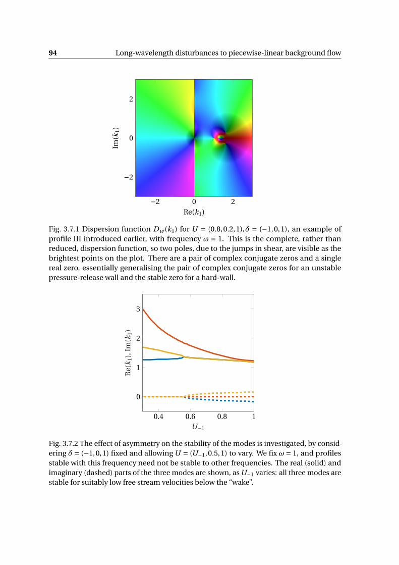
94 Long-wavelength disturbances to piecewise-linear background flow

−2 0 2

−2

0

2

Re(k1)

Im(k

1)

Fig. 3.7.1 Dispersion function Dw (k1) for U = (0.8,0.2,1),δ = (−1,0,1), an example ofprofile III introduced earlier, with frequency ω = 1. This is the complete, rather thanreduced, dispersion function, so two poles, due to the jumps in shear, are visible as thebrightest points on the plot. There are a pair of complex conjugate zeros and a singlereal zero, essentially generalising the pair of complex conjugate zeros for an unstablepressure-release wall and the stable zero for a hard-wall.

0.4 0.6 0.8 1

0

1

2

3

U−1

Re(

k1),

Im(k

1)

Fig. 3.7.2 The effect of asymmetry on the stability of the modes is investigated, by consid-ering δ= (−1,0,1) fixed and allowing U = (U−1,0.5,1) to vary. We fix ω= 1, and profilesstable with this frequency need not be stable to other frequencies. The real (solid) andimaginary (dashed) parts of the three modes are shown, as U−1 varies: all three modes arestable for suitably low free stream velocities below the “wake”.

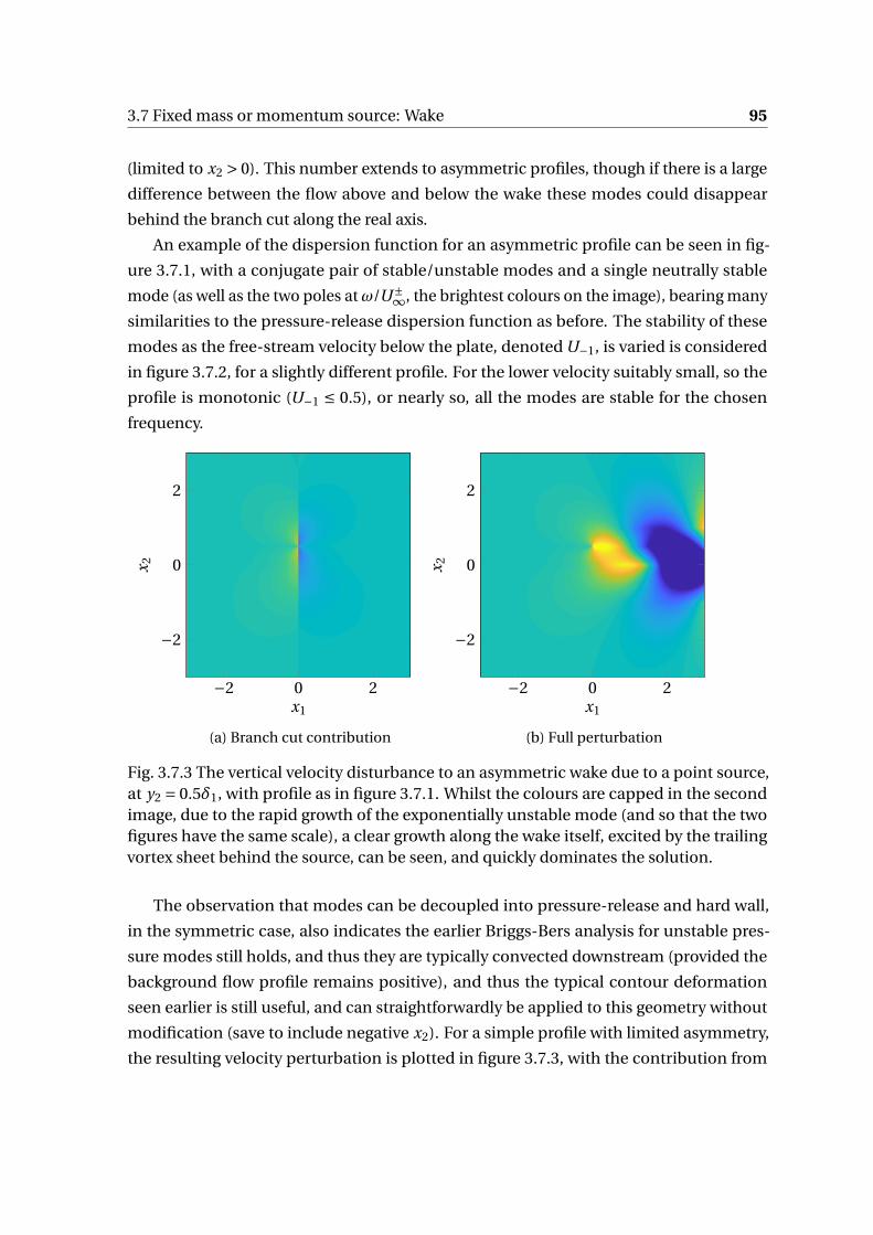
3.7 Fixed mass or momentum source: Wake 95

(limited to x2 > 0). This number extends to asymmetric profiles, though if there is a large

difference between the flow above and below the wake these modes could disappear

behind the branch cut along the real axis.

An example of the dispersion function for an asymmetric profile can be seen in fig-

ure 3.7.1, with a conjugate pair of stable/unstable modes and a single neutrally stable

mode (as well as the two poles atω/U±∞, the brightest colours on the image), bearing many

similarities to the pressure-release dispersion function as before. The stability of these

modes as the free-stream velocity below the plate, denoted U−1, is varied is considered

in figure 3.7.2, for a slightly different profile. For the lower velocity suitably small, so the

profile is monotonic (U−1 ≤ 0.5), or nearly so, all the modes are stable for the chosen

frequency.

−2 0 2

−2

0

2

x1

x 2

(a) Branch cut contribution

−2 0 2

−2

0

2

x1

x 2

(b) Full perturbation

Fig. 3.7.3 The vertical velocity disturbance to an asymmetric wake due to a point source,at y2 = 0.5δ1, with profile as in figure 3.7.1. Whilst the colours are capped in the secondimage, due to the rapid growth of the exponentially unstable mode (and so that the twofigures have the same scale), a clear growth along the wake itself, excited by the trailingvortex sheet behind the source, can be seen, and quickly dominates the solution.

The observation that modes can be decoupled into pressure-release and hard wall,

in the symmetric case, also indicates the earlier Briggs-Bers analysis for unstable pres-

sure modes still holds, and thus they are typically convected downstream (provided the

background flow profile remains positive), and thus the typical contour deformation

seen earlier is still useful, and can straightforwardly be applied to this geometry without

modification (save to include negative x2). For a simple profile with limited asymmetry,

the resulting velocity perturbation is plotted in figure 3.7.3, with the contribution from

96 Long-wavelength disturbances to piecewise-linear background flow

the branch cuts (either in the UHP for negative x1 or the LHP for positive x1) synthesised

without the modal excitation.

3.8 Discussion and conclusions

Previous work has shown that consideration of a constant-shear boundary-layer gives

rise to analytically tractable solutions to the equations governing long-wavelength per-

turbations, which can be matched to a radiating acoustic solution in the far-field. This

chapter has extended that work to more complicated boundary-layers, comprised of

intervals of constant shear, with careful matching conditions across the interfaces where

the background shear is discontinuous. This model lends itself to consideration of a point

mass source which, in agreement with a similar problem studied by Rienstra et al. [92],

generates a vortical and an acoustic disturbance in the presence of background shear.

This previous work noted a modal solution due to the presence of linear shear, a term

similarly found by Brambley et al. [22] in considering a similar problem in a curved duct,

though in the latter case work was required to separate this mode from the critical-layer

due to the curvature of the duct. This chapter has developed this theory, demonstrating

the presence of this modal solution is a natural consequence of a jump in background

shear. By increasing the number of junctions across which the background shear jumps,

there is a corresponding increase in the number of modal solutions. This should partially

serve as a warning with using broken-line profiles as approximations to profiles with

continuously varying shear, as the next chapter will investigate, with this modal solutions

not necessarily appearing in the latter case.

As noted in the introduction, the existence of surface modes, stable and unstable,

above a lined wall was identified by Rienstra and others in uniform flow [86, 87], and later

for sheared flow [111]. This work reproduces these results with surface modes naturally

dropping out of the analysis for lined walls, which in turn can be matched back to pressure-

release modes for Z = 0. The “outer” modes, corresponding to convective velocities further

away from the walls, are little changed by the introduction of a lined wall, maintaining

a similar location and structure to the hard-wall case, though the introduction of lining

can have a much greater effect on the “inner” modes. Further, we established that it is not

possible to cleanly identify pressure-release or hard-wall modes with impedance modes

as Z varies, since different modes disappear (either through a branch cut or to infinity)

depending on the argument of Z .

The quasi-numerical model developed in this chapter offers a rapid tool for computing

near field scattering from a mass source, though it is limited only to long-wavelength dis-

3.8 Discussion and conclusions 97

turbances, and rapidly loses numerical efficiency as the number of pieces, N , is increased.

The accuracy of this method is discussed in the next chapter. That said, it is possible to

use the results to calculate far-field noise directly, since analytic expressions for Fourier

transformed quantites exist. Whilst this work only considers the first-order far-field con-

tribution, via a limited application of Watson’s lemma, expansion of the Fourier inversion

integrand near k1 = 0 in a series would allow a complete asymptotic expansion of the

far-field sound as a sum of Hankel-type solutions to Helmholtz equation.

Two caveats must be mentioned, both considering the pressure-release (or impedance)

case when the background shear σ and the frequency ω are comparable. Two points jump

out: firstly that we cannot use the methods developed in this chapter to compute the

far-field sound, with seemingly infinite acoustic response developing. The second issue is

the emergence of “branch cut” modes, which are otherwise hidden on another Riemann

sheet of the complex plane. As has been demonstrated, an infinity of such modes occur as

ω→σ, and their effect is not completely understood. These two issues suggest this limit

should be investigated more closely, in particular understanding the physical mechanism

that leads to this singular behaviour.

The central aim of this chapter was to understand gust-like, rotational solutions to

Rayleigh’s equation in an analytically tractable limit. Through the identification of pref-

erentially excited modal solutions, we obtain a family of solutions convecting at a speed

beneath the free-stream velocity, regardless of the boundary condition being considered.

Given typical scattering models consider a gust-type harmonic solution convecting at

some prescribed convection velocity, beneath the free-stream velocity, we have a natural

theoretical determination of potential convection velocities, dependent on the physical

“location” of the modal solution within the boundary-layer.

The next chapter will develop a more comprehensive method for solving a similar

problem, which loses the analytic nicety of this method but is more generally applicable,

and allows revisiting of some potentially problematic results presented in this chapter, for

example the radiation above a pressure-release or impendance lining.

Chapter 4

Disturbances to continuously sheared

flow above a homogeneous boundary

The results of the previous chapter, §3, are extended to include an arbitrary continuous

background profile, allowing for variation of background density (or equivalently back-

ground speed of sound), inclusion of three-dimensional effects and direct inclusion of

compressibility in the perturbations. This allows analysis and development of the gust

solutions identified in the previous chapter, by focusing again on the acoustic disturbance

scattered from a point mass source.

4.1 Introduction

Whilst allowing for analytic solutions, the simplification of the Rayleigh equation in the

previous chapter neglects many of the physical effects contained within the full equation,

in particular the opportunity to directly consider compressible solutions. Relaxing these

assumptions requires numerical solution of the time-harmonic, streamwise transformed

Rayleigh equation, or its adjoint. Here, we focus on the adjoint equation as it gives rise

to a similar convected quantity as Orr’s equation (3.1.1), generalising the perturbation

vorticity, and therefore allows direct treatment of the wake of a point mass source.

Numerical solution of the (adjoint) compressible Rayleigh equation throws up new

difficulties that the previous formulation avoided with the need to carefully treat the

critical-layer [73, 22, 50]. For fixed streamwise wavenumber k1, there is a regular sin-

gular point of the differential equation wherever k1 = ω/U (x2). We primarily consider

monotonic boundary-layers, with U (0) and U (δ) =U∞ at the edge of the boundary-layer

(where δ could be infinite). The differential equation then has a regular singular point

100 Disturbances to continuously sheared flow above a homogeneous boundary

at x2 =U−1(ω/k1) if k1 ∈ (ω/U∞,ω/U0) (or k1 ∈ (ω/U0,ω/U∞) if the profile is decreasing

in x2). A standard quantity of interest is the (hard-wall) dispersion function, Dh =Vφd ,

which is the wall-normal velocity at the wall of the solution and decays as x2 →∞. This

can be computed by matching to φd at either the edge of the boundary-layer, or as x2 =∞,

using the fact that was can solve the governing differential equation in uniform flow. As

noted in the previous chapter, zeros of this dispersion function correspond to modal

solutions of the differential equation.

This dispersion function has a branch cut, in the streamwise wavenumber plane, along

k1 ∈ (ω/U∞,ω/U0), driven by the singular point. This can cause numerical difficulties

when evaluation near this critical-layer is required (for example when computing Fourier

inversion) or when the behaviour of functions on the critical-layer itself is of interest

(for example if there is a pole on the critical-layer. Previous work [22] has suggested a

Frobenius series-based approach, which allows for very precise solutions near the regular

singular point itself, where the solution is in some sense “known”, which can be matched

to integrated solutions either side of the critical point. The Frobenius series naturally

gives rise to a logarithmic term at this point, and theoretically the choice of the branch

cut of the logarithm allows some control of the location of the critical-layer. Whilst this is

practical when the background profile is linear, since there is only a single singular point,

it becomes more difficult for profiles that, if extended beyond the boundary-layer, would

be non-monotonic. An alternative method is outlined here, which instead integrates the

differential equation through the complex extension of physical coordinate x2. This allows

deformation of the branch cut as required, though it still connects the points ω/U∞ and

ω/U0. It also reduces the number of numerical points required, since evaluation of the

ODE solution near the critical-layer requires a very small step size to reduce error caused

by proximity to the singular point. The methods of these solutions are outlined in §4.2,

and the resulting strengths and weaknesses are analysed. This also allows evaluation of

the strength of the piecewise-linear methods, in the preceding chapter, as approximations

to more complicated profiles.

With this done, the point source problem is reintroduced, including direct evaluation

of the far-field sound through the method of steepest descent. This problem is primarily

considered as an introduction to the methods of Fourier inversion used in later chapters,

as well as to motivate the construction of gust solutions for scattering problems, permitting

rapid computation of the scattered solution in the near-field. The use of complex analytic

procedures, where appropriate, results in a solution that is independent of the grid being

evaluated on, which allows variation of output resolution with computational time directly

scaling with the number of evaluation points. When considering disturbances above

4.2 Solving the adjoint compressible Rayleigh equation 101

lined or pressure-release walls, the surface modes identified in the previous chapter

reemerge, and can indeed be associated with the hydrodynamic surface modes found

previously (with only minor effects from compressibility). The careful deformation of

Fourier inversion contours allows correct understanding of the propagation and growth of

these resulting surface modes, dealt with in §4.5. Finally, in §4.6, the previously outlined

methods are extended to consider disturbances above a wake, which requires extension

of the background flow field to be defined for all x2.

4.2 Solving the adjoint compressible Rayleigh equation

The name conventionally given to the governing equation varies depending on context. In

a cylindrical duct, the streamwise and azimuthally Fourier transformed/expanded form of

the pressure equation, (2.2.8), is typically referred to as the Pridmore-Brown equation [82].

In this section, we consider the temporal, streamwise and spanwise transformed version

of the adjoint equation (2.3.10) in a boundary-layer, resulting in a second order ordinary

differential equation (ODE) in the wall-normal coordinate x2. Whilst this bears many

similarities to the Pridmore-Brown equation, the rectilinear geometry (and thus removal

of terms like 1/r ) means we are, in practice, merely solving the compressible analogue

of the incompressible Rayleigh stability equation. In regions of uniform flow (and the

long-wavelength limit with uniform shear as seen in the previous chapter), this can be

solved analytically, and the solutions are developed below. High-frequency asymptotic

solutions are also readily attainable via the WKBJ method [1]. Both are then compared

to numerical methods of solving the equations, chosen to be efficient in variation of

the streamwise wavenumber k1: both brute-force Runge-Kutta integration across the

boundary-layer, and a Frobenius expansion-based method to properly understand the

behaviour of the equation near the critical point, when ω=U (x2)k1.

Methods for solution of both the direct and adjoint Rayleigh equation are essentially

analogous; in the Fourier transformed case reducing both to second-order differential

equations, linear in wall-normal coordinate x2, and the resulting modal solutions are

the same. This section focuses on the solution to the adjoint equation, as it is useful

for the work related to a point source disturbance later in the chapter, with a convected

disturbance trailing the source easily picked up through the adjoint formulation. How-

ever, in later chapters solution of the direct equation may be preferable (thereby directly

obtaining solutions for pressure, p, as function of transformation parameters ω,k1,k3),

in particular when the forcing term is streamwise homogeneous (such as far downstream

102 Disturbances to continuously sheared flow above a homogeneous boundary

from a source), and the methods outlined in this section must be suitably modified for the

equation DR013p013 = 0, which is a straightforward redefinition of ODE coefficients.

4.2.1 Preliminaries

We assume the background flow U and the density ρ0 (and thus the speed of sound c0)

depend only on the wall-normal coordinate x2. The general, transformed equation that

we are finding the solution to is

D†R013φ013 = 0. (4.2.1)

The untransformed adjoint Rayleigh operator can be written

D†R = D3

0 − c20

(∂2

1 +∂23

)D0 −∂2

(c2

0

(∂2 D0 +2U ′∂1

))=

[D3

0 − c20

(∂2

1 +∂23

)D0 −

(3U ′(c2

0)′+3U ′′c20

)∂1

]−

[(c2

0)′ D0 +4c20U ′∂1

]∂2 −

[c2

0 D0

]∂2

2

(4.2.2)

using D0 = D0/Dt and ∂i = ∂/∂xi to simplify notation. The extraction of the wall-normal

derivatives ∂2 allows the triply-transformed Rayleigh operator to be written as

D†R013 =

[C 3 + c2

0C(k2

1 +k23

)−

(3C ′(c2

0)′+3C ′′c20

)]−

[(c2

0)′C +4c20C ′

]∂2−

[c2

0C]∂2

2, (4.2.3)

with, as in §3.2, C = i (ω−U (x2)k1) the transformed convective operator, and thus C ′ =−iU ′k1. Division through by −c2

0C and rewriting the derivatives as total derivatives (since

everything is now a function of x2 alone) gives the ODE

d2φ

dx22

+[

(c20)′

c20

+ 4C ′

C

]dφ

dx2

+[

3(C ′c20)′

c20C

−(k2

1 +k23

)− C 2

c20

]φ= 0. (4.2.4)

If the background speed of sound is constant, this reduces further to

d2φ

dx22

+[

4C ′

C

]dφ

dx2

+[

3C ′′

C−

(k2

1 +k23

)− C 2

c20

]φ= 0. (4.2.5)

A useful fact that will be often used is that the Wronskian can be easily written down.

If we have two linearly independent solutions to (4.2.4), φ1 and φ2 then the Wronskian

W =φ1φ′2 −φ2φ

′1 satisfies the differential equation

dW

dx2

=−[

(c20)′

c20

+ 4C ′

C

]W (4.2.6)

4.2 Solving the adjoint compressible Rayleigh equation 103

with the term in square brackets exactly the leading coefficient of φ′ in the differential

equation. Noting it is exactly the derivative of log(c20C 4) allows solution of (4.2.6) as

W (x2) = W0

c20C 4

(4.2.7)

with W0 some constant that can be evaluated at a single location.

From φ, we can evaluate wall-normal velocity v ′ and pressure p ′, upon Fourier trans-

formation, as

p013 =−C 3φ013, (4.2.8a)

v013 =− 1

ρ0C

d

dx2

(C 3φ013

). (4.2.8b)

Auxiliary functions

The solution to the ODE is defined by any pair of linearly independent solutions (that is,

for which the derived Wronskian does not vanish), as any solution can be constructed

from a linear combination of them. However, for comparison between methods, and for

the later mathematical analysis, it is useful to focus on a well-defined pair of auxiliary

functions. For this purpose, we define φd and φh as the decaying and hard-wall solutions

respectively, with decaying solution

φd (x2) ∼ exp(−γ(k1,k3;U∞)x2

)x2 →∞ (4.2.9)

that is, the decaying solution in uniform flow (see definition of γ in (4.2.12) below), given

U (x2) → U∞ as x2 → ∞. The hard-wall solution is chosen so that the derived velocity

vh = 0 on x2 = 0. This leaves freedom to normalise φ, and thus ph is arbitrarily chosen to

be unity on x2 = 0. Mathematically

ph(0) = 1, (4.2.10a)

vh(0) = 0. (4.2.10b)

This is the solution above a hard-wall, with no particle displacement through x2 = 0. In

later analysis other auxiliary functions, tailored to different boundary conditions, will also

be considered, though they can always be written as a linear combination of φd and φh .

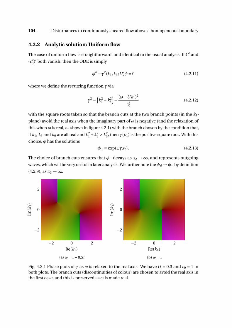
104 Disturbances to continuously sheared flow above a homogeneous boundary

4.2.2 Analytic solution: Uniform flow

The case of uniform flow is straightforward, and identical to the usual analysis. If C ′ and

(c20)′ both vanish, then the ODE is simply

φ′′−γ2(k1,k3;U )φ= 0 (4.2.11)

where we define the recurring function γ via

γ2 =(k2

1 +k23

)− (ω−Uk1)2

c20

(4.2.12)

with the square roots taken so that the branch cuts at the two branch points (in the k1-

plane) avoid the real axis when the imaginary part of ω is negative (and the relaxation of

this when ω is real, as shown in figure 4.2.1) with the branch chosen by the condition that,

if k1, k3 and k0 are all real and k21 +k2

3 > k20 , then γ(k1) is the positive square root. With this

choice, φ has the solutions

φ± = exp(±γx2). (4.2.13)

The choice of branch cuts ensures that φ− decays as x2 →∞, and represents outgoing

waves, which will be very useful in later analysis. We further note theφd →φ− by definition

(4.2.9), as x2 →∞.

−2 0 2

−2

0

2

Re(k1)

Im(k

1)

(a) ω= 1−0.5i

−2 0 2

−2

0

2

Re(k1)

Im(k

1)

(b) ω= 1

Fig. 4.2.1 Phase plots of γ as ω is relaxed to the real axis. We have U = 0.3 and c0 = 1 inboth plots. The branch cuts (discontinuities of colour) are chosen to avoid the real axis inthe first case, and this is preserved as ω is made real.

4.2 Solving the adjoint compressible Rayleigh equation 105

4.2.3 Numerical solution: Integration across boundary-layer

For fixed parameters and wavenumbers, it is relatively routine to find the numerical

solution to (4.2.4). Imposition of a condition either at infinity (in the decaying case, or if

considering perturbations to a wake) or at zero (in the hard-wall case, or other cases with

similarly prescribed boundary conditions) and recasting the differential equation into the

formdΦ

dx2

= F(x2,Φ(x2);ω,k1,k3) (4.2.14)

allows implementation of routine Runge-Kutta or similar methods.

The simplest approach is to takeΦ1 =φ andΦ2 =φ′, which gives simply

F1 =Φ2 (4.2.15a)

F2 =−qΦ1 −pΦ2 (4.2.15b)

with p and q , functions of x2, derived from the governing equation as in (4.2.22) (and not

to be confused with pressure fluctuations). In terms ofΦ= (Φ1,Φ2), the derived physical

quantites are

p013 =−C 3Φ1 (4.2.16a)

v013 =−3c20C ′CΦ1 − c2

0C 2Φ2 (4.2.16b)

which can be used to set hard-wall and pressure-release boundary conditions in terms of

Φ. If we have U constant outside some region 0 < x2 < δ, then the decaying and hard-wall

boundary conditions are, respectively

(Φ1)d (δ) = exp(−γ∞δ) (Φ2)d (δ) =(−γ∞− 3C ′∞

C∞exp(−γ∞δ)

), (4.2.17)

(Φ1)h(0) =− 1

C 30

(Φ2)h(0) = 3C ′0

C 40

. (4.2.18)

Subscript ∞ implies evaluation at x2 = δ and subscript 0 at x2 = 0. Note: this imposes a

choice of branch cut on φd , driven by the behaviour at infinity, through γ∞. This, as the

asymptotic consideration above, leads to some interesting behaviour as the branch points

of γ change as x2 varies.

For fixed k1, it is straightforward to use inbuilt integration routines to compute the

differential equation solution, for example Matlab’s ode45, which uses a variable-step

mixed RK4/RK5 routine. Varying k1 can be done by a simple loop over values of k1 which

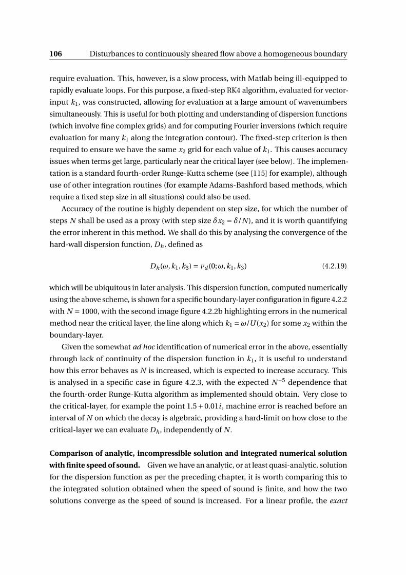
106 Disturbances to continuously sheared flow above a homogeneous boundary

require evaluation. This, however, is a slow process, with Matlab being ill-equipped to

rapidly evaluate loops. For this purpose, a fixed-step RK4 algorithm, evaluated for vector-

input k1, was constructed, allowing for evaluation at a large amount of wavenumbers

simultaneously. This is useful for both plotting and understanding of dispersion functions

(which involve fine complex grids) and for computing Fourier inversions (which require

evaluation for many k1 along the integration contour). The fixed-step criterion is then

required to ensure we have the same x2 grid for each value of k1. This causes accuracy

issues when terms get large, particularly near the critical layer (see below). The implemen-

tation is a standard fourth-order Runge-Kutta scheme (see [115] for example), although

use of other integration routines (for example Adams-Bashford based methods, which

require a fixed step size in all situations) could also be used.

Accuracy of the routine is highly dependent on step size, for which the number of

steps N shall be used as a proxy (with step size δx2 = δ/N ), and it is worth quantifying

the error inherent in this method. We shall do this by analysing the convergence of the

hard-wall dispersion function, Dh , defined as

Dh(ω,k1,k3) = vd (0;ω,k1,k3) (4.2.19)

which will be ubiquitous in later analysis. This dispersion function, computed numerically

using the above scheme, is shown for a specific boundary-layer configuration in figure 4.2.2

with N = 1000, with the second image figure 4.2.2b highlighting errors in the numerical

method near the critical layer, the line along which k1 =ω/U (x2) for some x2 within the

boundary-layer.

Given the somewhat ad hoc identification of numerical error in the above, essentially

through lack of continuity of the dispersion function in k1, it is useful to understand

how this error behaves as N is increased, which is expected to increase accuracy. This

is analysed in a specific case in figure 4.2.3, with the expected N−5 dependence that

the fourth-order Runge-Kutta algorithm as implemented should obtain. Very close to

the critical-layer, for example the point 1.5+0.01i , machine error is reached before an

interval of N on which the decay is algebraic, providing a hard-limit on how close to the

critical-layer we can evaluate Dh , independently of N .

Comparison of analytic, incompressible solution and integrated numerical solution

with finite speed of sound. Given we have an analytic, or at least quasi-analytic, solution

for the dispersion function as per the preceding chapter, it is worth comparing this to

the integrated solution obtained when the speed of sound is finite, and how the two

solutions converge as the speed of sound is increased. For a linear profile, the exact

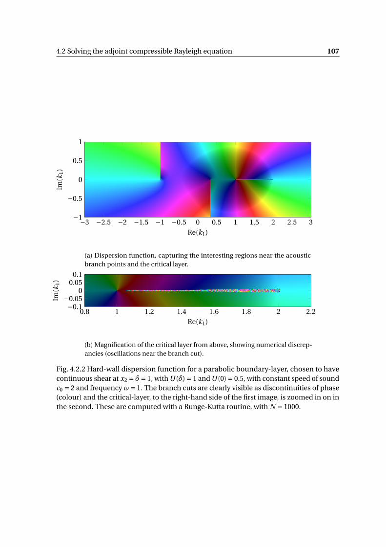
4.2 Solving the adjoint compressible Rayleigh equation 107

−3 −2.5 −2 −1.5 −1 −0.5 0 0.5 1 1.5 2 2.5 3−1

−0.5

0

0.5

1

Re(k1)

Im(k

1)

(a) Dispersion function, capturing the interesting regions near the acousticbranch points and the critical layer.

0.8 1 1.2 1.4 1.6 1.8 2 2.2−0.1

−0.050

0.050.1

Re(k1)

Im(k

1)

(b) Magnification of the critical layer from above, showing numerical discrep-ancies (oscillations near the branch cut).

Fig. 4.2.2 Hard-wall dispersion function for a parabolic boundary-layer, chosen to havecontinuous shear at x2 = δ= 1, with U (δ) = 1 and U (0) = 0.5, with constant speed of soundc0 = 2 and frequency ω= 1. The branch cuts are clearly visible as discontinuities of phase(colour) and the critical-layer, to the right-hand side of the first image, is zoomed in on inthe second. These are computed with a Runge-Kutta routine, with N = 1000.

108 Disturbances to continuously sheared flow above a homogeneous boundary

100 101 102 103 10410−15

10−9

10−3

103

109

Integration points, N = 1/(δx2)

Rel

ativ

eer

ror,|D

h(k

1,N

)−D

h(k

1,N

∞)|

k1 =−1k1 = 0k1 = 0+1ik1 = 3k1 = 10k1 = 1.5+0.1ik1 = 1.5+0.05ik1 = 1.5+0.01i

Fig. 4.2.3 The convergence of the numerical routine, computing Dh at arbitrary values ofk1, as number of integration points, N , is increased. This is compared to evaluation atN = N∞ = 105, where the total error of the routine is dominated by machine error, and thecomputed solution merely fluctuates around some constant value. A simple parabolicprofile with U0 = 0.5 and U∞ = 1, with c0 = 2 constant, is used, for frequencyω= 1, thoughthis result is general. The slope is −5 when the above plot is linear, as would be expectedfor a fourth-order Runge-Kutta algorithm, for all values of k1 chosen until machine errordominates, after which the error is broadly constant. The only difference is points nearthe critical-layer, here with k1 = 1.5+ iϵ for various ϵ, where N must be sufficiently highfor the error to decay, with the required N increasing as ϵ decreases, and if ϵ is sufficientlysmall there is a bound on accuracy.

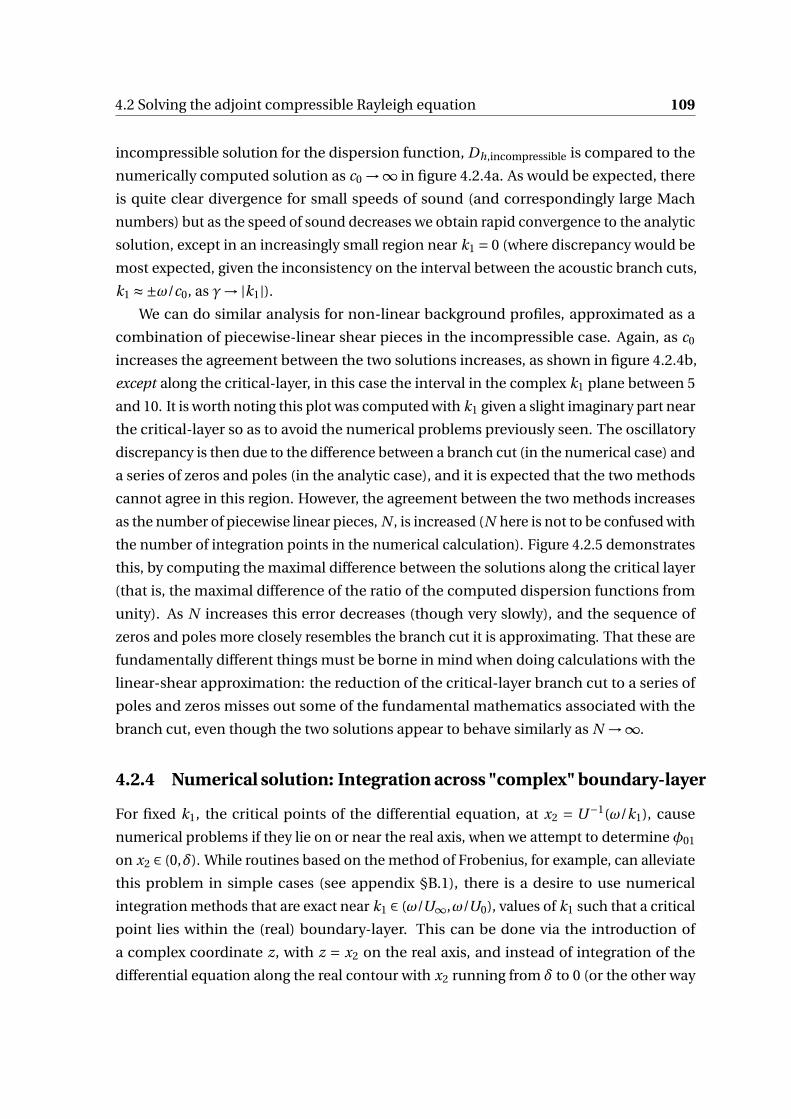
4.2 Solving the adjoint compressible Rayleigh equation 109

incompressible solution for the dispersion function, Dh,incompressible is compared to the

numerically computed solution as c0 →∞ in figure 4.2.4a. As would be expected, there

is quite clear divergence for small speeds of sound (and correspondingly large Mach

numbers) but as the speed of sound decreases we obtain rapid convergence to the analytic

solution, except in an increasingly small region near k1 = 0 (where discrepancy would be

most expected, given the inconsistency on the interval between the acoustic branch cuts,

k1 ≈±ω/c0, as γ→|k1|).

We can do similar analysis for non-linear background profiles, approximated as a

combination of piecewise-linear shear pieces in the incompressible case. Again, as c0

increases the agreement between the two solutions increases, as shown in figure 4.2.4b,

except along the critical-layer, in this case the interval in the complex k1 plane between 5

and 10. It is worth noting this plot was computed with k1 given a slight imaginary part near

the critical-layer so as to avoid the numerical problems previously seen. The oscillatory

discrepancy is then due to the difference between a branch cut (in the numerical case) and

a series of zeros and poles (in the analytic case), and it is expected that the two methods

cannot agree in this region. However, the agreement between the two methods increases

as the number of piecewise linear pieces, N , is increased (N here is not to be confused with

the number of integration points in the numerical calculation). Figure 4.2.5 demonstrates

this, by computing the maximal difference between the solutions along the critical layer

(that is, the maximal difference of the ratio of the computed dispersion functions from

unity). As N increases this error decreases (though very slowly), and the sequence of

zeros and poles more closely resembles the branch cut it is approximating. That these are

fundamentally different things must be borne in mind when doing calculations with the

linear-shear approximation: the reduction of the critical-layer branch cut to a series of

poles and zeros misses out some of the fundamental mathematics associated with the

branch cut, even though the two solutions appear to behave similarly as N →∞.

4.2.4 Numerical solution: Integration across "complex" boundary-layer

For fixed k1, the critical points of the differential equation, at x2 = U−1(ω/k1), cause

numerical problems if they lie on or near the real axis, when we attempt to determine φ01

on x2 ∈ (0,δ). While routines based on the method of Frobenius, for example, can alleviate

this problem in simple cases (see appendix §B.1), there is a desire to use numerical

integration methods that are exact near k1 ∈ (ω/U∞,ω/U0), values of k1 such that a critical

point lies within the (real) boundary-layer. This can be done via the introduction of

a complex coordinate z, with z = x2 on the real axis, and instead of integration of the

differential equation along the real contour with x2 running from δ to 0 (or the other way

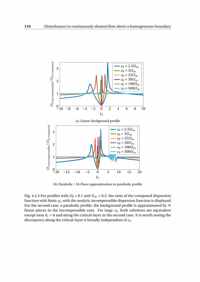
110 Disturbances to continuously sheared flow above a homogeneous boundary

−10 −8 −6 −4 −2 0 2 4 6 8 100

1

2

3

k1

Dh

,inco

mp

ress

ible

/Dh

,co

mp

ute

d

c0 = 2.5U∞c0 = 5U∞c0 = 25U∞c0 = 50U∞c0 = 100U∞c0 = 500U∞

(a) Linear background profile

−20 −15 −10 −5 0 5 10 15 200

1

2

3

k1

Dh

,inco

mp

ress

ible

/Dh

,co

mp

ute

d

c0 = 2.5U∞c0 = 5U∞c0 = 25U∞c0 = 50U∞c0 = 100U∞c0 = 500U∞

(b) Parabolic / 10-Piece approximation to parabolic profile

Fig. 4.2.4 For profiles with U0 = 0.1 and U∞ = 0.2, the ratio of the computed dispersionfunction with finite c0, with the analytic incompressible dispersion function is displayed.For the second case, a parabolic profile, the background profile is approximated by Nlinear pieces in the incompressible case. For large c0, both solutions are equivalentexcept near k1 = 0 and along the critical-layer in the second case. It is worth noting thediscrepency along the critical-layer is broadly independent of c0.

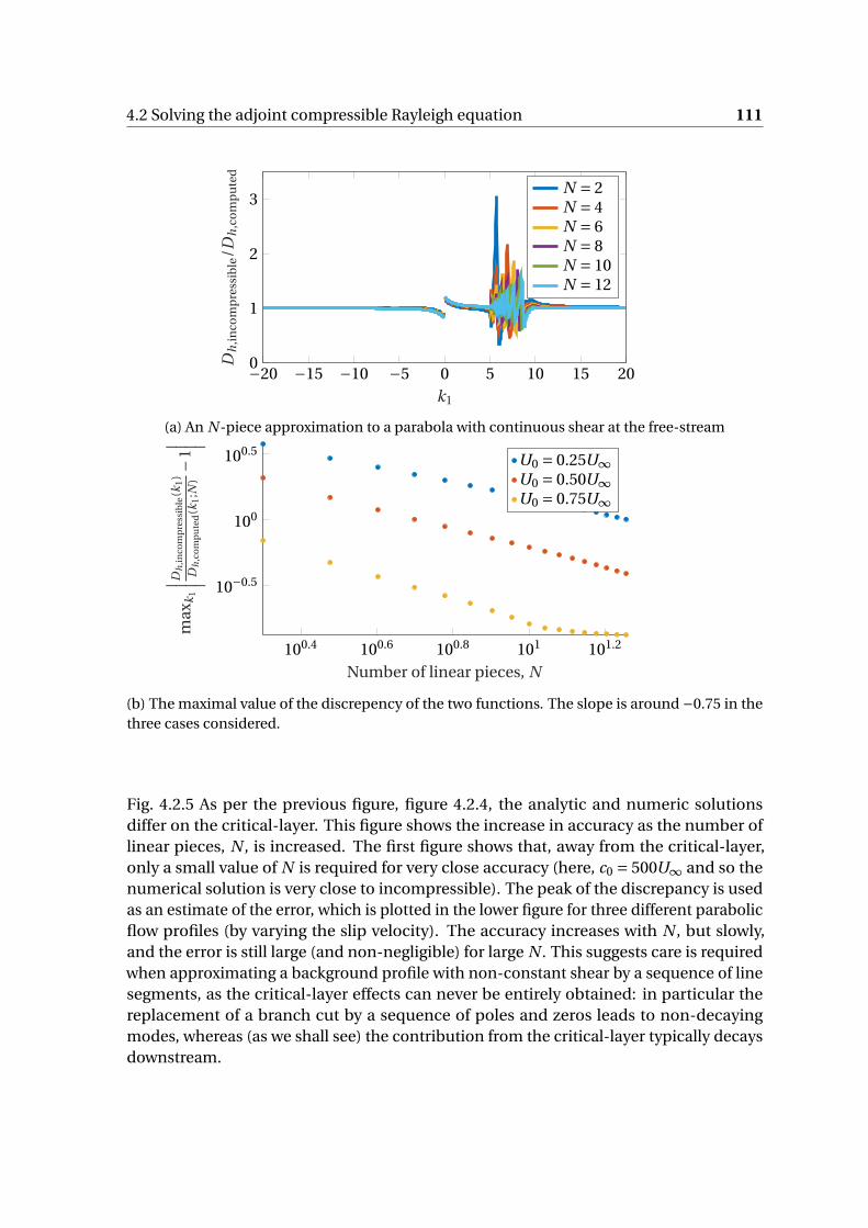
4.2 Solving the adjoint compressible Rayleigh equation 111

−20 −15 −10 −5 0 5 10 15 200

1

2

3

k1

Dh

,inco

mp

ress

ible

/Dh

,co

mp

ute

d

N = 2N = 4N = 6N = 8N = 10N = 12

(a) An N -piece approximation to a parabola with continuous shear at the free-stream

100.4 100.6 100.8 101 101.2

10−0.5

100

100.5

Number of linear pieces, N

max

k1

∣ ∣ ∣ ∣Dh

,inco

mp

ress

ible

(k1

)D

h,c

om

pu

ted

(k1

;N)−1

∣ ∣ ∣ ∣

U0 = 0.25U∞U0 = 0.50U∞U0 = 0.75U∞

(b) The maximal value of the discrepency of the two functions. The slope is around −0.75 in thethree cases considered.

Fig. 4.2.5 As per the previous figure, figure 4.2.4, the analytic and numeric solutionsdiffer on the critical-layer. This figure shows the increase in accuracy as the number oflinear pieces, N , is increased. The first figure shows that, away from the critical-layer,only a small value of N is required for very close accuracy (here, c0 = 500U∞ and so thenumerical solution is very close to incompressible). The peak of the discrepancy is usedas an estimate of the error, which is plotted in the lower figure for three different parabolicflow profiles (by varying the slip velocity). The accuracy increases with N , but slowly,and the error is still large (and non-negligible) for large N . This suggests care is requiredwhen approximating a background profile with non-constant shear by a sequence of linesegments, as the critical-layer effects can never be entirely obtained: in particular thereplacement of a branch cut by a sequence of poles and zeros leads to non-decayingmodes, whereas (as we shall see) the contribution from the critical-layer typically decaysdownstream.

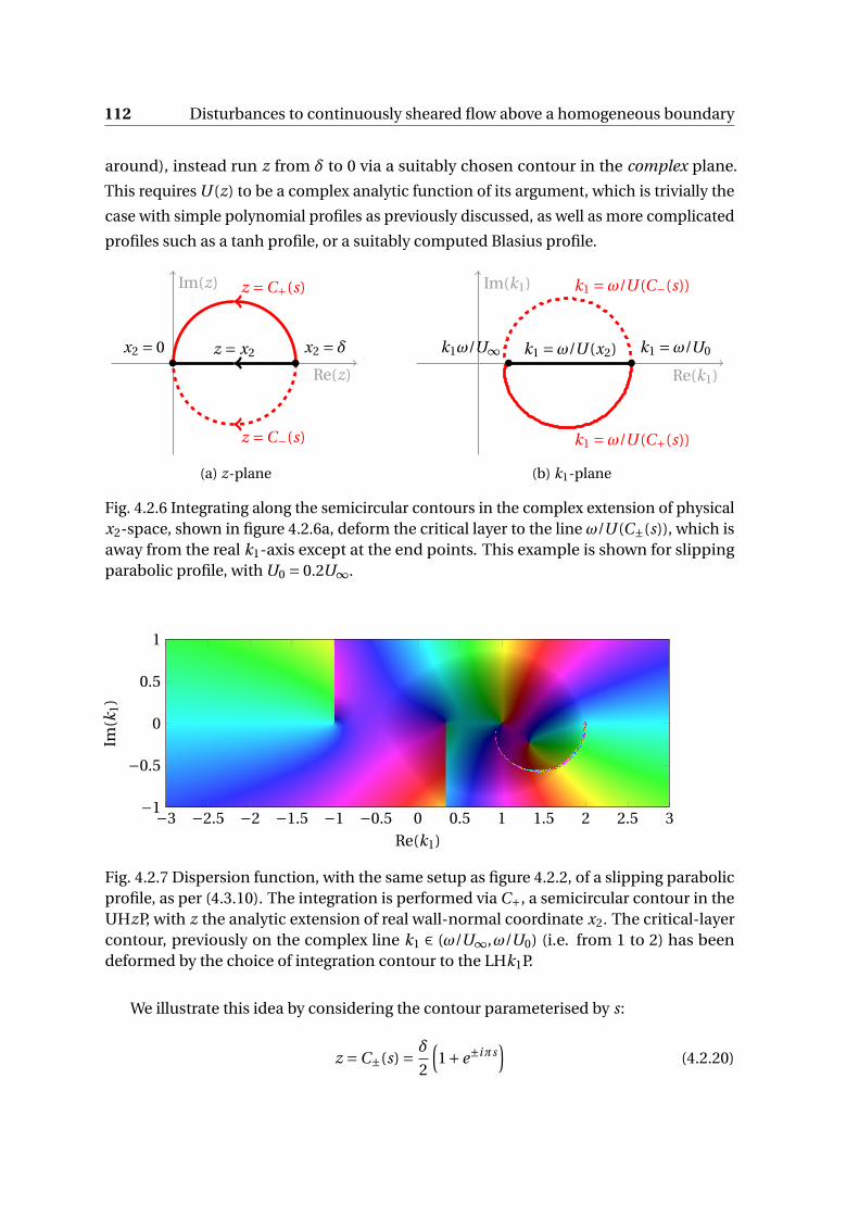
112 Disturbances to continuously sheared flow above a homogeneous boundary

around), instead run z from δ to 0 via a suitably chosen contour in the complex plane.

This requires U (z) to be a complex analytic function of its argument, which is trivially the

case with simple polynomial profiles as previously discussed, as well as more complicated

profiles such as a tanh profile, or a suitably computed Blasius profile.

Re(z)

Im(z)

z = x2

z =C+(s)

z =C−(s)

x2 = 0 x2 = δ

(a) z-plane

Re(k1)

Im(k1)

k1 =ω/U (x2)

k1 =ω/U (C−(s))

k1 =ω/U (C+(s))

k1ω/U∞ k1 =ω/U0

(b) k1-plane

Fig. 4.2.6 Integrating along the semicircular contours in the complex extension of physicalx2-space, shown in figure 4.2.6a, deform the critical layer to the line ω/U (C±(s)), which isaway from the real k1-axis except at the end points. This example is shown for slippingparabolic profile, with U0 = 0.2U∞.

−3 −2.5 −2 −1.5 −1 −0.5 0 0.5 1 1.5 2 2.5 3−1

−0.5

0

0.5

1

Re(k1)

Im(k

1)

Fig. 4.2.7 Dispersion function, with the same setup as figure 4.2.2, of a slipping parabolicprofile, as per (4.3.10). The integration is performed via C+, a semicircular contour in theUHzP, with z the analytic extension of real wall-normal coordinate x2. The critical-layercontour, previously on the complex line k1 ∈ (ω/U∞,ω/U0) (i.e. from 1 to 2) has beendeformed by the choice of integration contour to the LHk1P.

We illustrate this idea by considering the contour parameterised by s:

z =C±(s) = δ

2

(1+e±iπs

)(4.2.20)

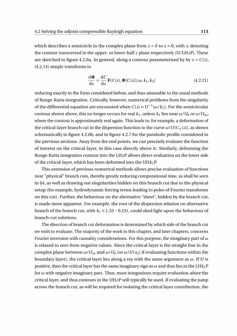
4.2 Solving the adjoint compressible Rayleigh equation 113

which describes a semicircle in the complex plane from z = δ to z = 0, with ± denoting

the contour transversed in the upper- or lower-half z plane respectively (U/LHzP). These

are sketched in figure 4.2.6a. In general, along a contour parameterised by by z =C (s),

(4.2.14) simply transforms to

dΦ

ds= dC

dsF(C (s),Φ(C (s));ω,k1,k3) (4.2.21)

reducing exactly to the form considered before, and thus amenable to the usual methods

of Runge-Kutta integration. Critically, however, numerical problems from the singularity

of the differential equation are encounted when C (s) ≈U−1(ω/k1). For the semicircular

contour shown above, this no longer occurs for real k1, unless k1 lies near ω/U0 or ω/U∞,

where the contour is approximately real again. This leads to, for example, a deformation of

the critical-layer branch cut in the dispersion function to the curve ω/U (C±(s)), as shown

schematically in figure 4.2.6b, and in figure 4.2.7 for the parabolic profile considered in

the previous sections. Away from the end points, we can precisely evaluate the function

of interest on the critical-layer, in this case directly above it. Similarly, deforming the

Runge-Kutta integration contour into the LHzP allows direct evaluation on the lower side

of the critical-layer, which has been deformed into the UHk1P.

This extension of previous numerical methods allows precise evaluation of functions

near "physical" branch cuts, thereby greatly reducing computational time, as shall be seen

in §4, as well as drawing out singularities hidden on this branch cut due to the physical

setup (for example, hydrodynamic forcing terms leading to poles of Fourier transforms

on this cut). Further, the behaviour on the alternative “sheet”, hidden by the branch cut,

is made more apparent. For example, the root of the dispersion relation on alternative

branch of the branch cut, with k1 ≈ 1.33−0.23i , could shed light upon the behaviour of

branch-cut solutions.

The direction of branch cut deformation is determined by which side of the branch cut

we wish to evaluate. The majority of the work in this chapter, and later chapters, concerns

Fourier inversion with causality considerations. For this purpose, the imaginary part of ω

is relaxed to zero from negative values. Since the critical layer is the straight line in the

complex plane between ω/U∞ and ω/U0 (or ω/U (x2) if evaluating functions within the

boundary layer), the critical layer lies along a ray with the same argument as ω. If U is

positive, then the critical layer has the same imaginary sign asω and thus lies in the LHk1P

for ω with negative imaginary part. Thus, most integrations require evaluation above the

critical layer, and thus contours in the UHzP will typically be used. If evaluating the jump

across the branch cut, as will be required for isolating the critical layer contribution, the

114 Disturbances to continuously sheared flow above a homogeneous boundary

cut can be deformed into the LHk1P when evaluating at k1 + i 0 in the UHk1P, and vice

versa. This allows very precise evaluation either side of the branch cut, with comparatively

little numerical expense.

4.2.5 Asymptotic solution: High frequency acoustics

For high frequency, short-wavelength disturbances, a routine application of the WKBJ

method allows determination of the asymptotic behavior of the solution, with arbitrary

boundary-layer and density profiles. This allows verification of the numerical methods

for higher frequencies, allows understanding of the large k1 behaviour of the dispersion

function (important in the scattering later) and provides a simple framework for analytic

progress. The WKBJ process assumes the wall-normal wavelength is much shorter than

the boundary-layer thickness (and thus, in some sense, the solution is determined by the

local background flow speed as opposed local background shear).

We begin by working (4.2.4) into canonical form, a step that isn’t necessary but simpli-

fies the analysis. We write the ODE as

d2φ

dx22

+p(x2)dφ

dx2

+q(x2)φ= 0 (4.2.22)

with p(x2) = log(c2

0C 4)′

and q(x2) = 3(C ′c20)′/(c2

0C )−γ(k1,k3;U (x2))2, as determined above.

We remove the first derivative term by posing φ= AΦ, with A(x2) to be determined. If

1

A

d A

dx2

=−p

2(4.2.23)

then the equation forΦ is of the form

d2Φ

dx22

+Q(x2)Φ= 0 (4.2.24)

with

Q(x2) = A′′

A− p2

2+q. (4.2.25)

Since the integral of p is known (returning the Wronskian), we can integrate the equation

for A to obtain

A(x2) = 1

c0C 2. (4.2.26)

At the moment this is simply a direct reformulation of the ODE for φ, and nothing has

actually been done. It is now that we suppose the frequency, ω, is in some sense large. We

4.2 Solving the adjoint compressible Rayleigh equation 115

first note that the dominant wavenumbers of interest scale broadly with ω, so if ω is large

then so is k1 (and possibly k3). We use k1 to define a small lengthscale ϵ= k−11 . Defining

O(1) quantities

Ω= ϵω (4.2.27a)

Ki = ϵki (4.2.27b)

Γ= ϵγ=√

K 21 +K 2

3 − (Ω−U (x2)K1)2/c0(x2)2 (4.2.27c)

then we can rewrite Q, grouping terms by powers of ϵ,

Q(x2) = −Γ2(K1,K3;U (x2))

ϵ2+O(ϵ0). (4.2.28)

The local effects of mean flow (encapsulated in the acoustic exponent Γ) dominate the

local effects of shear (contained within −p2/2 and A′′/A in (4.2.25)). Positing a solution to

(4.2.24) of the form

Φ= exp

(ϵ−1

∞∑n=0

ϵnSn(x2)

)(4.2.29)

allows equating of functions at each order in ϵ, by putting this into the ODE (4.2.24)1. The

first order equations are

S′0

2 = Γ2 (4.2.30a)

2S′0S′

1 +S′′0 = 0 (4.2.30b)

with no O(ϵ−1) contribution from Q(x2) in the second equation, and primes denoting x2

derivatives. This is exactly the method and solution in Bender and Orzsag [14], with these

equations respectively the eikonal and transport equations. We can solve to give

S0 =±∫ x2

Γ(K1,K3,U (x2))dx2, (4.2.31a)

S1 = log(±Γ−1/2

), (4.2.31b)

giving a pair of solutions, asymptotically correct to O(1) in ϵ:

φ± ∼ 1

γ1/2c0C 2exp

(±

∫γ(x2)dx2

). (4.2.32)

1There is no a priori reason to expand in ϵ itself, rather than some function of ϵ (for example ϵ1/2), otherthan knowledge of the final solution.

116 Disturbances to continuously sheared flow above a homogeneous boundary

Explicit dependence on the somewhat fabricated ϵ has been dropped, though it should be

understood this is only strictly valid for high frequencies or wavenumbers. This solution

trivially becomes the uniform flow solution when U is constant, as expected. The pressure

and wall-normal velocity perturbation fields can be derived as

v± ∼−C 2φ′ ∼∓γ1/2

c0exp

(±

∫γ(x2)dx2

), (4.2.33a)

p± ∼−C 3φ∼− C

γ1/2c0exp

(±

∫γ(x2)dx2

), (4.2.33b)

Both are continuous over discontinuities of U ′, since γ is continuous (if not differentiable).

It remains to validate this solution, which we can do via a comparison with the pre-

ceding numerical solution. In particular, we wish to show that these solutions are asymp-

totically equivalent to the exact solution as k1 → ∞, even for moderate ω, a property

which will be important in the scattering analysis in later chapters. As before, we use the

hard-wall dispersion function as validation, for which we require

φd ∼ γ1/2(δ)c0(δ)C (δ)2

γ1/2(x2)c0(x2)C (x2)2exp

(∫ δ

x2

γ(s)ds −γ(δ)δ

)(4.2.34)

with the scaling constants chosen to ensure φd ∼ exp(−γx2) for x2 > δ. The dispersion

function is then asymptotically

Dh ∼ γ1/2(δ)γ1/2(0)c0(δ)C (δ)2

c0(0)exp

(∫ δ

0γ(s)ds −γ(δ)δ

). (4.2.35)

For very simple profiles it is possible to do the integral

I =∫ δ

0

√k2

1 +k23 − c−2

0 (s)(ω2 −k1U (s))2 ds (4.2.36)

exactly in terms of elementary functions, and it is straightforward to compute for more

complicated profiles numerically.

By way of validation, the asymptotic dispersion function is compared to the computed

dispersion function, with very small step size, along the real k1 axis in figure 4.2.8. This

comparison could be done across any ray in the complex k1-plane with similar results.

As the log-plot, figure 4.2.8b shows, the difference between the computed and precise

solutions decays like k−11 , as would be expected from the asymptotic analysis. This vali-

dation allows numerical computations to be replaced by the comparatively trivial WKBJ

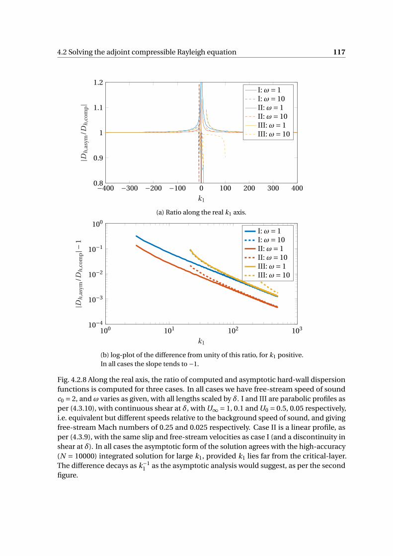
4.2 Solving the adjoint compressible Rayleigh equation 117

−400 −300 −200 −100 0 100 200 300 4000.8

0.9

1

1.1

1.2

k1

|Dh

,asy

m/D

h,c

om

p|

I: ω= 1I: ω= 10II: ω= 1II: ω= 10III: ω= 1III: ω= 10

(a) Ratio along the real k1 axis.

100 101 102 10310−4

10−3

10−2

10−1

100

k1

|Dh

,asy

m/D

h,c

om

p|−

1

I: ω= 1I: ω= 10II: ω= 1II: ω= 10III: ω= 1III: ω= 10

(b) log-plot of the difference from unity of this ratio, for k1 positive.In all cases the slope tends to −1.

Fig. 4.2.8 Along the real axis, the ratio of computed and asymptotic hard-wall dispersionfunctions is computed for three cases. In all cases we have free-stream speed of soundc0 = 2, and ω varies as given, with all lengths scaled by δ. I and III are parabolic profiles asper (4.3.10), with continuous shear at δ, with U∞ = 1, 0.1 and U0 = 0.5, 0.05 respectively,i.e. equivalent but different speeds relative to the background speed of sound, and givingfree-stream Mach numbers of 0.25 and 0.025 respectively. Case II is a linear profile, asper (4.3.9), with the same slip and free-stream velocities as case I (and a discontinuity inshear at δ). In all cases the asymptotic form of the solution agrees with the high-accuracy(N = 10000) integrated solution for large k1, provided k1 lies far from the critical-layer.The difference decays as k−1

1 as the asymptotic analysis would suggest, as per the secondfigure.

118 Disturbances to continuously sheared flow above a homogeneous boundary

solution for large k1, which will be critical when the scattering problem is considered in

later chapters.

4.3 A point mass source in continuous shear

The work of §3, specifically from sections 3.4.1 onwards, is generalised to more arbitrary

background profile U (x2). Other than the supposition that the profile is continuous, this

can be prescribed as desired, though we expect instability for inflecting profiles. Again,

we consider the setup of a harmonic mass source in shear flow, generating a vortical

disturbance in its wake, and consider both the downstream development of disturbances

and the far-field acoustics from the source. The generic setup is shown in figure 4.3.1,

which will be revisited and the relevant lengthscales discussed in section 4.4.2.

x2

x1

Lφ= 0

q0

U =U∞

δ

λh

λa

y2

Fig. 4.3.1 Schematic of the setup of this section, highlighting the four lengthscales ofinterest: the boundary-layer thickness δ, source location y2, and the two scattered length-scales, corresponding to hydrodynamic motion in the boundary-layer (λh) and acousticdisturbances propagating to the far-field (λa).

This generalisation, allowing finite speed of sound and (somewhat) arbitrary wave-

lengths and thus including the effects of incompressibility, gives rise to the existence of a

critical-layer. Whilst this can be dealt with and removed via the inclusion of viscosity, we

focus on the inviscid case and thus the effects of the critical-layer must be studied directly.

Recall (2.3.10), governing the evolution of a generalised velocity potential for acoustic

disturbances. With a mass source q(x, t ), we have

D0

Dt

(D†

Rφ)= c2

0 q (4.3.1)

with the adjoint Rayleigh operator given by

D†R = D3

0

Dt 3− ∂

∂xi

c20

(∂

∂xi

D0

Dt+2

∂U

∂xi

∂

∂x1

) . (4.3.2)

4.3 A point mass source in continuous shear 119

If we again consider a point mass source, q = q0e iωtδ(x1)δ(x2 − y2), we obtain, exactly

analogously to (3.4.6), a partial differential equation for φ:

D†Rφ= c0(y2)2q0

U (y2)δ(x2 − y2)H(x1)exp

(−iκ1(y2)x1)

. (4.3.3)

In the long-wavelength, constant shear case, the perturbation vorticity was confined to a

streamline starting at the source. This solution extends this to a more generalised vortical

quantity, confined again to a streamline, which drives the evolution of the pertubation

quantites. For streamwise homogenous boundary condition on x2 = 0, Lφ= 0 for some

linear operator L which doesn’t depend on x1 or x3, we can solve using Fourier transforms

as before to give

φ013 = c0(y2)2q0

U (y2)

1

i (k1 −κ1)

1

W (y2)

φd (x2)φℓ(y2) x2 > y2

φℓ(x2)φd (x2) x2 < y2(4.3.4)

with φd ∼ exp(−γ∞(k1,k3)x2) as x2 →∞, and L013φℓ = 0 on x2 = 0, with both auxiliary

functions satisfying the ODE

D†R013φ013 = 0 (4.3.5)

with solution as discussed in §4.2. As yet, other than the constants in front q0, this is

unchanged from §3.4.1. The difference in the constants follows from the consideration of

a different potential, φ here as opposed to ψ previously. As noted in (4.2.7), the Wronskian

is not constant in this case. Provided the inner solution φℓ is scaled analogously to

the previous section, so that W (x2 = 0) = Dℓ(ω,k1,k3),the dispersion function given by

L013φd (x2 = 0), then

W (y2) = c0(0)2C (0)4

c0(y2)2C (y2)4Dℓ (4.3.6)

with C (x2) = i (ω−U (x2)k1) as usual. If the boundary condition is written ℓ1φ′ℓ+ℓ2φℓ = 0,

this setup requires

φℓ(0) = ℓ1, (4.3.7a)

φ′ℓ(0) =−ℓ2. (4.3.7b)

Both sides of this implicitly depend on k1 (and the other parameters). If a different

normalisation is chosen, this must be included in the Wronskian (and so it cancels out).

120 Disturbances to continuously sheared flow above a homogeneous boundary

We can therefore write down the time-harmonic solution

φ03 = 1

2πi

c0(y2)4q0

c0(0)2

∫F1

C (y2;k1)4φ≷(x2;k1)φ≶(y2;k1)

C (0;k1)4Dℓ(k1)

e−i k1x1

k1 −κ1dk1. (4.3.8)

The conventions in the previous chapter are maintained, with φ≷(x2) given by φd (x2) for

x2 > y2 and φℓ for x2 < y2. The Fourier inversion contour is deformed off the real k1 axis

so as to preserve causality as the imaginary part of ω is relaxed to zero. Deformation of

this contour to a semicircle at infinity will pick up not only contributions from any poles,

and from the acoustic branch cuts, but also from the hydrodynamic branch cut of the

critical layer. As before, it is sensible to consider this with an explicit choice of boundary

condition, which we shall do in the following section.

Typically from here on, we will consider straightforward polynomial background

boundary-layer profiles, with linear profile given by (for x2 < δ)

U (x2) =U0 + (U∞−U0)x2

δ(4.3.9)

and parabolic profile, with continuous shear at the edge of the boundary-layer, given by

U (x2) =U∞− (U∞−U0)

(1− x2

δ

)2

. (4.3.10)

In both cases, the slip velocity U0 =U (0) and the boundary-layer is matched to a constant

profile U =U∞ for x2 > δ. In this work the speed of sound is typically a constant, with

c0 >U∞ >U0, though the model allows variation of background speed of sound (through

variations in background density), a simplification justified in the derivation §2 for low

Mach-number flows. If not explicit, lengths will be scaled by boundary-layer thickness δ

and speeds by the free-stream velocity U∞, equivalently setting δ=U∞ = 1.

4.3.1 Far-field noise: Steepest descent

For x2 > δ, outside the boundary-layer, or as x2 →∞ if we take the boundary-layer to

be infinitely thick, we recall we defined φd ∼ exp(−γ∞x2), thereby putting the inversion

integral into the form

φ03 =∫

F1

Iℓ(k1)exp(−i k1x1 −γ∞x2)dk1 (4.3.11)

4.3 A point mass source in continuous shear 121

with Iℓ depending on the boundary-conditions and various physical parameters. For the

point mass source, we have

Iℓ =1

2πi

c0(y2)4q0

c0(0)2

C (y2;k1)4

C (0;k1)4

φℓ(y2;k1)

Dℓ(k1)

1

k1 −κ1(y2)(4.3.12)

and derivatives can be computed via ∂/∂x1 = −i k1 and (outwith the boundary layer)

∂/∂x2 =−γ∞.

Along the real axis, or near the real axis, this integral is oscillatory, driven by the

Fourier inversion factor e−i k1x1 . The ideal contour to integrate along is the steepest descent

contour, on which the exponent has constant imaginary part, and thereby the integral

is (essentially) non-oscillatory. For r = |x|≫ δ, the rapid decay of this exponent, along a

suitably chosen contour, allows asymptotic approximation of the integral from a single

saddle point contribution.

Suppose we are at an observation point (x1, x2) such that x1 = R cos(Θ) and βx2 =R sin(Θ), where we introduce

β=√

1−M 2∞ (4.3.13)

with the far-field Mach number M∞ =U∞(δ)/c0(δ) (or a similarly defined limit at infinity),

and we introduce the acoustic wavenumber k0 = ω/c0(δ) similarly, with the length of

acoustic waves, in the free-stream, given by its reciprocal. The reason for the introduction

of β is to reduce the following calculation, and can be considered a Doppler-shift effect.

The integral outside the boundary-layer then looks like

φ03 =∫

F1

Iℓ(k1)exp(−R f (k1;Θ))dk1 (4.3.14)

where we define the exponent

f (k1;Θ) = i k1 cos(Θ)+β−1γ∞(k1)sin(Θ) (4.3.15)

where γ2∞ = k21 +k2

3 − (k0 −k1M∞)2. If we now introduce new wavenumbers

K1 = k1 + M∞k0

β2(4.3.16a)

K 20 = k2

0

β4− k2

3

β2(4.3.16b)

122 Disturbances to continuously sheared flow above a homogeneous boundary

and rearrange, we obtain

f =− i M∞k0

β2cos(Θ)+ i K1 cos(Θ)+

√K 2

1 −K 20 sin(Θ) (4.3.17)

The first term is constant and doesn’t effect the computation of the steepest descent

contour, and so we focus on

F (K1;Θ) = i K1 cos(Θ)+√

K 21 −K 2

0 sin(Θ) (4.3.18)

which is identical to the zero-velocity, spanwise invariant case if k1 = K1 and K0 = k0,

essentially we have corrected for mean flow (and cross-flow variations), which can be

compared to the Prandtl-Glauert transformation [39]. In this case we could have K 20 < 0

due to the presence of k3 terms, which must be treated carefully.

The error, due to oscillations, is minimised if a contour is chosen that passes through

a saddle point of this exponent [52]. The best contour to choose is the one on which the

imaginary part of F is constant, which can be determined parametrically for givenΘ. First

noting saddle points are located at zeros of F ′, with

F ′ = i cos(Θ)+ K1√K 2

1 −K 20

sin(Θ) (4.3.19)

which has a single zero when K1 = K1s = K0 cos(Θ) (with care being required with the

sign of this solution, which results from the choice of branch cuts of γ and the imaginary

part of ω), and as such we want the contour passing through this point with Im(F (K1)) =Im(F (K1s)) = K0. This is most cleanly done via the substitution K1 = K0 cosh(u) =K0 cosh(ur+i ui ), which gives

Im(F ) = K0 cosh(ur )[cos(Θ)cos(ui )+ sin(Θ)sin(ui )

]= cosh(ur )cos(θ−ui ) = K0 (4.3.20)

Choosing to parameterise by t = − tanh(ur ) we can write down the steepest descent

contour, as a function of t , via

K1SD (t ;Θ) = K0

(cos(Θ)+ tp

1− t 2sin(Θ)

)+ i

(− t 2

p1− t 2

cos(Θ)+ t sin(Θ)

) (4.3.21)

with t running from −1 to 1, and K1SD tending towards complex infinity in two different

directions at either endpoint. This parameterisation has the advantage that it a finite

integral in t , and thus a useful substitution for numerical integration, as well as removing

4.3 A point mass source in continuous shear 123

ambiguity about the square root. The change of variables gives

dk1 = dK1 = 1

(1− t 2)3/2sin(Θ)+ i

(t (t 2 −2)

(1− t 2)3/2cos(Θ)+ sin(Θ)

)dt (4.3.22)

which is singular as t →±1, though the exponential decay of the integrand makes this

unimportant. The saddle point is now located at t = 0 where dk1 = k0(1+ i )sin(Θ)dt .

This contour is useful to integrate along even when R is not large, for example just out-

side the boundary-layer, and we further make the assumption it is a reasonable integration

contour for x2 < δ, as the exponential behaviour isn’t greatly changed. For Rk0 ≫ 1, we

can determine the first-order asymptotic behaviour of the contour integral via Laplace’s

method, with the saddle point dominating. This might not be the first-order contribution

to the entire integral, with contributions from the deformation to the steepest descent

contour to be expected, particularly from poles at roots of the relevant dispersion relation.

The steepest descent integral is of the form

J =∫ 1

−1I (t )e−RG(t ) dt (4.3.23)

with G(t ) = F (K1SD (t ))−F (K1SD (0)) a real function of t , and I (t ) complex and well-behaved

along the contour (with integrable singularities at the end points that we will for now

ignore). G(t ) is minimal when t = 0, and the vicinity of this global minimum dominates

the integral for R large (which can be made explicit via, for example, Watson’s lemma

[112], compare §4.4.2). Near t = 0, G(t) ≈ K0t 2, the simplicity of this expression again

supporting the choice of definition of t . Locally we consider the integral

Jϵ =∫ ϵ

−ϵI (t )e−RK0t 2

dt ∼∫ p

K0Rϵ

−pRK0ϵ

I (0)pRK0

e−u2du ∼ I (0)

√π

RK0(4.3.24)

with ϵ small but finite, in the limit RK0 →∞. This contribution is a cylindrical wave, driven

by the value of I at the saddle point.

In terms of the earlier Iℓ(k1) (equation (4.3.12)) and the physical parameters, this

contribution is (recalling the various extra factors, including the change of variable contri-

bution)

Iℓ

((k2

0 −β2k23)1/2

β2

x1

(x21 +β2x2

2)1/2

)x2(2iπ)1/2(k2

0 −β2k23)1/4

(x21 +β2x2

2)3/4exp

[i x1

β2

(M∞k0 − (k2

0 −β2k23)1/2

)](4.3.25)

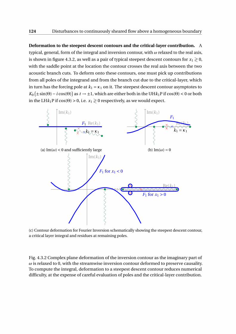
124 Disturbances to continuously sheared flow above a homogeneous boundary

Deformation to the steepest descent contours and the critical-layer contribution. A

typical, general, form of the integral and inversion contour, with ω relaxed to the real axis,

is shown in figure 4.3.2, as well as a pair of typical steepest descent contours for x1 ≷ 0,

with the saddle point at the location the contour crosses the real axis between the two

acoustic branch cuts. To deform onto these contours, one must pick up contributions

from all poles of the integrand and from the branch cut due to the critical-layer, which

in turn has the forcing pole at k1 = κ1 on it. The steepest descent contour asymptotes to

K0(±sin(Θ)− i cos(Θ)

)as t →±1, which are either both in the UHk1P if cos(Θ) < 0 or both

in the LHk1P if cos(Θ) > 0, i.e. x1 ≷ 0 respectively, as we would expect.

Re(k1)

Im(k1)

k1 = κ1

F1

(a) Im(ω) < 0 and sufficiently large

Re(k1)

Im(k1)

k1 = κ1

F1

(b) Im(ω) = 0

Re(k1)

Im(k1)

F1 for x1 > 0

F1 for x1 < 0

(c) Contour deformation for Fourier Inversion schematically showing the steepest descent contour,a critical layer integral and residues at remaining poles.

Fig. 4.3.2 Complex plane deformation of the inversion contour as the imaginary part ofω is relaxed to 0, with the streamwise inversion contour deformed to preserve causality.To compute the integral, deformation to a steepest descent contour reduces numericaldifficulty, at the expense of careful evaluation of poles and the critical-layer contribution.

4.4 Hard-wall boundaries 125

4.4 Hard-wall boundaries

With any singularities of the dispersion function, and thus the integrand, confined to

the real k1 axis, the case of a point source above a hard-wall boundary is easiest to deal

with, with no additional modal contributions aside from those contained within the

critical layer integral. We impose the boundary condition that V0013φ013 = 0, explicitly

corresponding to ℓ1 =−C 2, ℓ2 =−3CC ′, both evaluated at x2 = 0, which corresponds to

imposing the perturbations having no wall-normal velocity at the wall, and thus there is

no fluid penetration through the surface.

The dispersion function for this problem is shown in figures 4.4.1, for both a linear

and parabolic background profile, as computed using the standard techniques from §4.2,

and hence leading to numerical discrepancies near the critical layer (in this case, with

U0 = 0.3 and U∞ = 1, and unit frequency ω= 1, the interval k1 ∈ (1,3.33) on the real axis).

However, it can be seen that the critical layer in the linear case is removable (in that the

argument of Dh does not jump across it), which is not true in the parabolic case. This

leads to fundamental differences in the computed solution: as in the piecewise linear case,

the linear case gives rise to propagating modes, whereas the parabolic case gives rise to an

algebraically decaying contribution.

Also shown in figures 4.4.1 are the integration contours to be used to evaluate this

inversion. Two things are worth noting here: whilst the "branch cut" contours CU ,P ,

extending into the U/LHk1P and centred around the branch points of γ∞, resemble the

Steepest Descent contours, they need not be exactly the same. This reduces the need

for the contours to depend on x1 and x2, the physical coordinates, and vastly speeds

up computation time, though the steepest descent contour (and resulting saddle point

contribution) is useful for evaluating the far-field contribution from this integral, and fewer

points are needed for convergence if the contour goes through or near the saddle point.

Secondly, the critical-layer contribution is evaluated explicitly via an integral around the

branch cut. This is done due to the presence of poles on the branch cut itself: if they did not

exist, or utilisation of a principal valued integral was worthwhile, the critical layer integral

could be reduced to a single integral along the contour (with arbitrary precision attained

by deforming the physical integration path in the real plane so that the critical layer moves

away from the contour of integration). This is done to evaluate the downstream behaviour

of this contribution later.

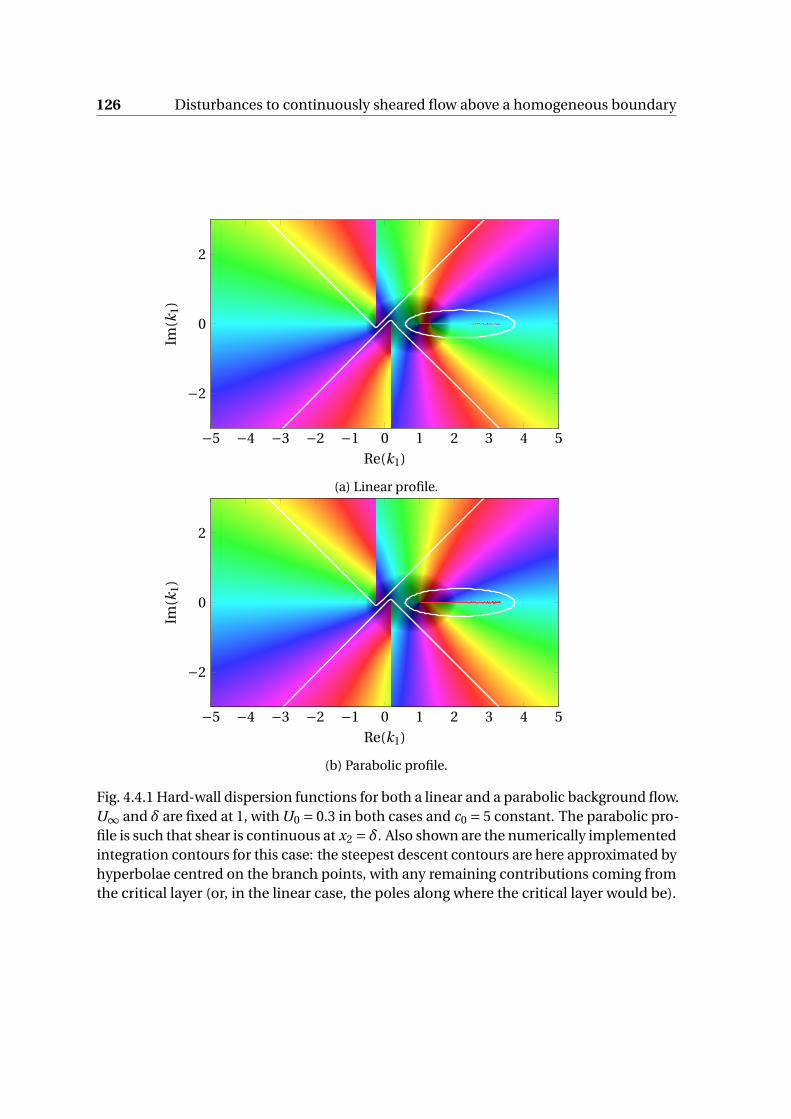
126 Disturbances to continuously sheared flow above a homogeneous boundary

−5 −4 −3 −2 −1 0 1 2 3 4 5

−2

0

2

Re(k1)

Im(k

1)

(a) Linear profile.

−5 −4 −3 −2 −1 0 1 2 3 4 5

−2

0

2

Re(k1)

Im(k

1)

(b) Parabolic profile.

Fig. 4.4.1 Hard-wall dispersion functions for both a linear and a parabolic background flow.U∞ and δ are fixed at 1, with U0 = 0.3 in both cases and c0 = 5 constant. The parabolic pro-file is such that shear is continuous at x2 = δ. Also shown are the numerically implementedintegration contours for this case: the steepest descent contours are here approximated byhyperbolae centred on the branch points, with any remaining contributions coming fromthe critical layer (or, in the linear case, the poles along where the critical layer would be).

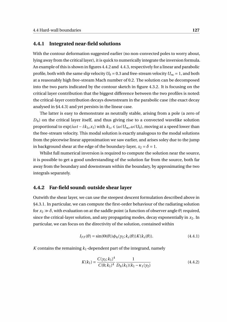
4.4 Hard-wall boundaries 127

4.4.1 Integrated near-field solutions

With the contour deformation suggested earlier (no non-convected poles to worry about,

lying away from the critical layer), it is quick to numerically integrate the inversion formula.

An example of this is shown in figures 4.4.2 and 4.4.3, respectively for a linear and parabolic

profile, both with the same slip velocity U0 = 0.3 and free-stream velocity U∞ = 1, and both

at a reasonably high free-stream Mach number of 0.2. The solution can be decomposed

into the two parts indicated by the contour sketch in figure 4.3.2. It is focusing on the

critical layer contribution that the biggest difference between the two profiles is noted:

the critical-layer contribution decays downstream in the parabolic case (the exact decay

analysed in §4.4.3) and yet persists in the linear case.

The latter is easy to demonstrate as neutrally stable, arising from a pole (a zero of

Dh) on the critical layer itself, and thus giving rise to a convected wavelike solution

proportional to exp(iωt − i k1c x1) with k1c ∈ (ω/U∞,ω/U0), moving at a speed lower than

the free-stream velocity. This modal solution is exactly analogous to the modal solutions

from the piecewise linear approximation we saw earlier, and arises soley due to the jump

in background shear at the edge of the boundary-layer, x2 = δ= 1.

Whilst full numerical inversion is required to compute the solution near the source,

it is possible to get a good understanding of the solution far from the source, both far

away from the boundary and downstream within the boundary, by approximating the two

integrals separately.

4.4.2 Far-field sound: outside shear layer

Outwith the shear layer, we can use the steepest descent formulation described above in

§4.3.1. In particular, we can compute the first-order behaviour of the radiating solution

for x2 ≫ δ, with evaluation on at the saddle point (a function of observer angle θ) required,

since the critical-layer solution, and any propagating modes, decay exponentially in x2. In

particular, we can focus on the directivity of the solution, contained within

IF F (θ) = sin(Θ(θ))φh(y2;ks(θ))K (ks(θ)). (4.4.1)

K contains the remaining k1-dependent part of the integrand, namely

K (k1) = C (y2;k1)4

C (0;k1)4

1

Dh(k1)(k1 −κ1(y2)(4.4.2)

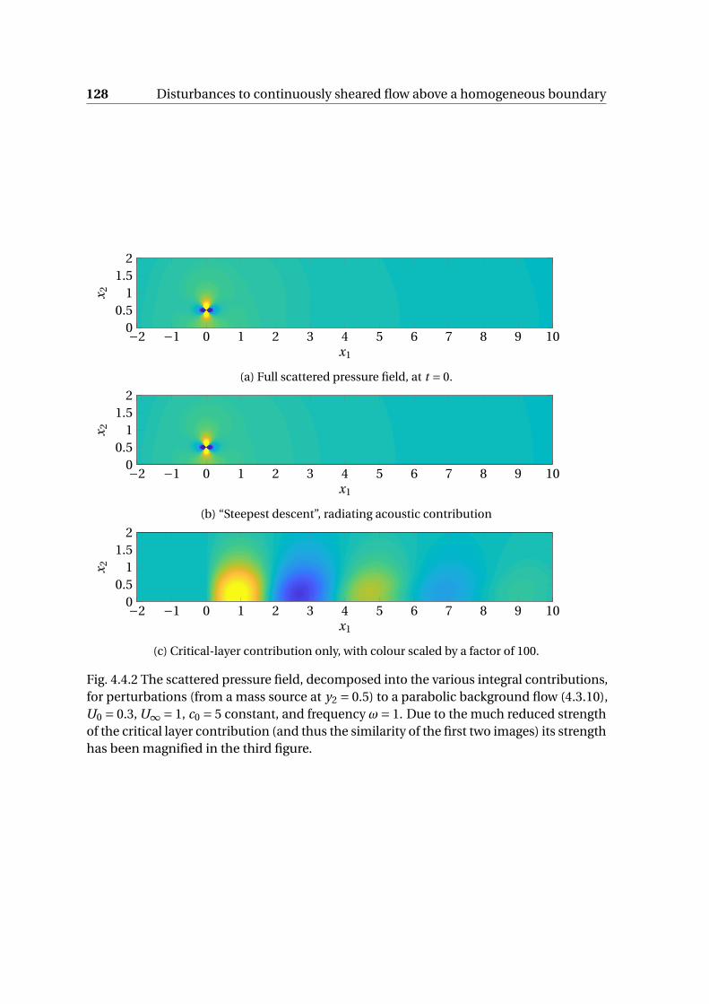
128 Disturbances to continuously sheared flow above a homogeneous boundary

−2 −1 0 1 2 3 4 5 6 7 8 9 100

0.51

1.52

x1

x 2

(a) Full scattered pressure field, at t = 0.

−2 −1 0 1 2 3 4 5 6 7 8 9 100

0.51

1.52

x1

x 2

(b) “Steepest descent”, radiating acoustic contribution

−2 −1 0 1 2 3 4 5 6 7 8 9 100

0.51

1.52

x1

x 2

(c) Critical-layer contribution only, with colour scaled by a factor of 100.

Fig. 4.4.2 The scattered pressure field, decomposed into the various integral contributions,for perturbations (from a mass source at y2 = 0.5) to a parabolic background flow (4.3.10),U0 = 0.3, U∞ = 1, c0 = 5 constant, and frequency ω= 1. Due to the much reduced strengthof the critical layer contribution (and thus the similarity of the first two images) its strengthhas been magnified in the third figure.

4.4 Hard-wall boundaries 129

−2 −1 0 1 2 3 4 5 6 7 8 9 100

0.51

1.52

x1

x 2

(a) Full scattered pressure field, at t = 0.

−2 −1 0 1 2 3 4 5 6 7 8 9 100

0.51

1.52

x1

x 2

(b) “Steepest descent”, radiating acoustic contribution

−2 −1 0 1 2 3 4 5 6 7 8 9 100

0.51

1.52

x1

x 2

(c) Critical-layer contribution only, with colour scaled by a factor of 100.

Fig. 4.4.3 The scattered pressure field, decomposed into the various integral contributions,for perturbations (from a mass source at y2 = 0.5) to a linear background flow (4.3.9),U0 = 0.3, U∞ = 1, c0 = 5 constant, and frequency ω= 1. The major difference between thisimage and figure 4.4.2 is that the critical layer does not decay downstream.

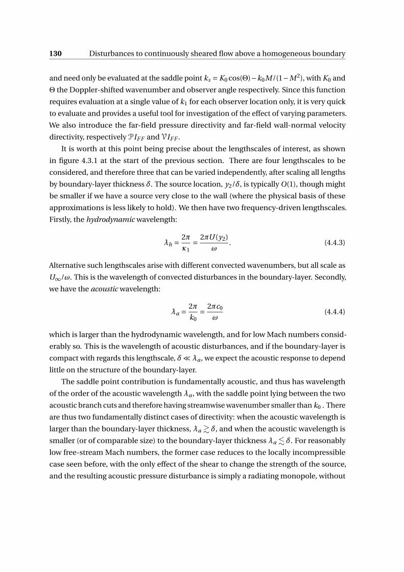
130 Disturbances to continuously sheared flow above a homogeneous boundary

and need only be evaluated at the saddle point ks = K0 cos(Θ)−k0M/(1−M 2), with K0 and

Θ the Doppler-shifted wavenumber and observer angle respectively. Since this function

requires evaluation at a single value of k1 for each observer location only, it is very quick

to evaluate and provides a useful tool for investigation of the effect of varying parameters.

We also introduce the far-field pressure directivity and far-field wall-normal velocity

directivity, respectively PIF F and VIF F .

It is worth at this point being precise about the lengthscales of interest, as shown

in figure 4.3.1 at the start of the previous section. There are four lengthscales to be

considered, and therefore three that can be varied independently, after scaling all lengths

by boundary-layer thickness δ. The source location, y2/δ, is typically O(1), though might

be smaller if we have a source very close to the wall (where the physical basis of these

approximations is less likely to hold). We then have two frequency-driven lengthscales.

Firstly, the hydrodynamic wavelength:

λh = 2π

κ1= 2πU (y2)

ω. (4.4.3)

Alternative such lengthscales arise with different convected wavenumbers, but all scale as

U∞/ω. This is the wavelength of convected disturbances in the boundary-layer. Secondly,

we have the acoustic wavelength:

λa = 2π

k0= 2πc0

ω(4.4.4)

which is larger than the hydrodynamic wavelength, and for low Mach numbers consid-

erably so. This is the wavelength of acoustic disturbances, and if the boundary-layer is

compact with regards this lengthscale, δ≪λa , we expect the acoustic response to depend

little on the structure of the boundary-layer.

The saddle point contribution is fundamentally acoustic, and thus has wavelength

of the order of the acoustic wavelength λa , with the saddle point lying between the two

acoustic branch cuts and therefore having streamwise wavenumber smaller than k0 . There

are thus two fundamentally distinct cases of directivity: when the acoustic wavelength is

larger than the boundary-layer thickness, λa & δ, and when the acoustic wavelength is

smaller (or of comparable size) to the boundary-layer thickness λa . δ. For reasonably

low free-stream Mach numbers, the former case reduces to the locally incompressible

case seen before, with the only effect of the shear to change the strength of the source,

and the resulting acoustic pressure disturbance is simply a radiating monopole, without

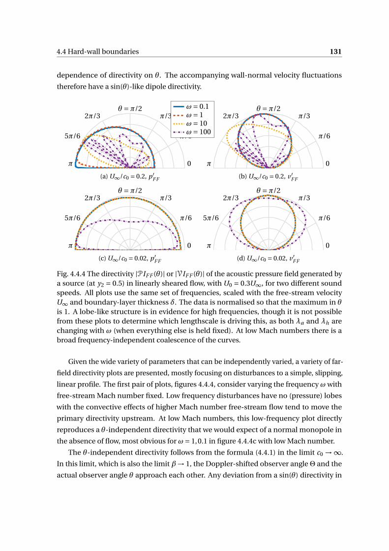
4.4 Hard-wall boundaries 131

dependence of directivity on θ. The accompanying wall-normal velocity fluctuations

therefore have a sin(θ)-like dipole directivity.

0

π/6

π/3θ =π/2

π

5π/6

2π/3ω= 0.1ω= 1ω= 10ω= 100

(a) U∞/c0 = 0.2, p ′F F

0

π/6

π/3θ =π/2

π

2π/3

(b) U∞/c0 = 0.2, v ′F F

0

π/6

π/3θ =π/2

π

5π/6

2π/3

(c) U∞/c0 = 0.02, p ′F F

0

π/6

π/3θ =π/2

π

5π/6

2π/3

(d) U∞/c0 = 0.02, v ′F F

Fig. 4.4.4 The directivity |PIF F (θ)| or |VIF F (θ)| of the acoustic pressure field generated bya source (at y2 = 0.5) in linearly sheared flow, with U0 = 0.3U∞, for two different soundspeeds. All plots use the same set of frequencies, scaled with the free-stream velocityU∞ and boundary-layer thickness δ. The data is normalised so that the maximum in θ

is 1. A lobe-like structure is in evidence for high frequencies, though it is not possiblefrom these plots to determine which lengthscale is driving this, as both λa and λh arechanging with ω (when everything else is held fixed). At low Mach numbers there is abroad frequency-independent coalescence of the curves.

Given the wide variety of parameters that can be independently varied, a variety of far-

field directivity plots are presented, mostly focusing on disturbances to a simple, slipping,

linear profile. The first pair of plots, figures 4.4.4, consider varying the frequency ω with

free-stream Mach number fixed. Low frequency disturbances have no (pressure) lobes

with the convective effects of higher Mach number free-stream flow tend to move the

primary directivity upstream. At low Mach numbers, this low-frequency plot directly

reproduces a θ-independent directivity that we would expect of a normal monopole in

the absence of flow, most obvious for ω= 1,0.1 in figure 4.4.4c with low Mach number.

The θ-independent directivity follows from the formula (4.4.1) in the limit c0 →∞.

In this limit, which is also the limit β→ 1, the Doppler-shifted observer angleΘ and the

actual observer angle θ approach each other. Any deviation from a sin(θ) directivity in

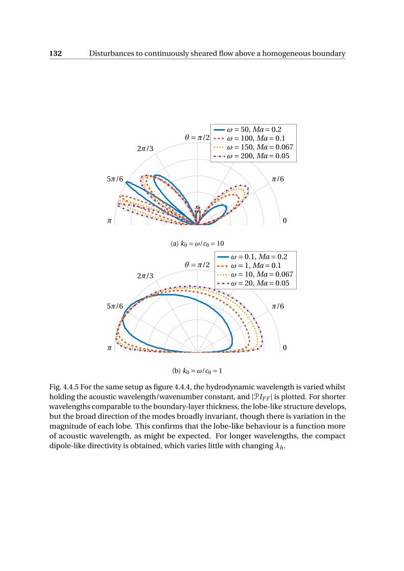
132 Disturbances to continuously sheared flow above a homogeneous boundary

0

π/6

π/3

θ =π/2

π

5π/6

2π/3

ω= 50, Ma = 0.2ω= 100, Ma = 0.1ω= 150, Ma = 0.067ω= 200, Ma = 0.05

(a) k0 =ω/c0 = 10

0

π/6

π/3

θ =π/2

π

5π/6

2π/3

ω= 0.1, Ma = 0.2ω= 1, Ma = 0.1ω= 10, Ma = 0.067ω= 20, Ma = 0.05

(b) k0 =ω/c0 = 1

Fig. 4.4.5 For the same setup as figure 4.4.4, the hydrodynamic wavelength is varied whilstholding the acoustic wavelength/wavenumber constant, and |PIF F | is plotted. For shorterwavelengths comparable to the boundary-layer thickness, the lobe-like structure develops,but the broad direction of the modes broadly invariant, though there is variation in themagnitude of each lobe. This confirms that the lobe-like behaviour is a function moreof acoustic wavelength, as might be expected. For longer wavelengths, the compactdipole-like directivity is obtained, which varies little with changing λh .

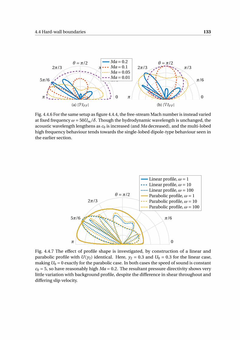
4.4 Hard-wall boundaries 133

0

π/6

π/3θ =π/2

π

5π/6

2π/3Ma = 0.2Ma = 0.1Ma = 0.05Ma = 0.01

(a) |PIF F |0

π/6

π/3θ =π/2

π

2π/3

(b) |VIF F |

Fig. 4.4.6 For the same setup as figure 4.4.4, the free-stream Mach number is instead variedat fixed frequency ω= 50U∞/δ. Though the hydrodynamic wavelength is unchanged, theacoustic wavelength lengthens as c0 is increased (and Ma decreased), and the multi-lobedhigh frequency behaviour tends towards the single-lobed dipole-type behaviour seen inthe earlier section.

0

π/6

π/3θ =π/2

π

5π/6

2π/3

Linear profile, ω= 1Linear profile, ω= 10Linear profile, ω= 100Parabolic profile, ω= 1Parabolic profile, ω= 10Parabolic profile, ω= 100

Fig. 4.4.7 The effect of profile shape is investigated, by construction of a linear andparabolic profile with U (y2) identical. Here, y2 = 0.3 and U0 = 0.3 for the linear case,making U0 = 0 exactly for the parabolic case. In both cases the speed of sound is constantc0 = 5, so have reasonably high Ma = 0.2. The resultant pressure directivity shows verylittle variation with background profile, despite the difference in shear throughout anddiffering slip velocity.

134 Disturbances to continuously sheared flow above a homogeneous boundary

0

π/6

π/3θ =π/2

π

5π/6

2π/3y2 = 0.25y2 = 0.50y2 = 0.75

(a) ω= 10

0

π/6

π/3θ =π/2

π

5π/6

2π/3

(b) ω= 50

Fig. 4.4.8 For the same setup as figure 4.4.4 with fixed speed of sound c0 = 5. |PIF F | isplotted for two chosen frequencies: ω= 10 so the acoustic wavelength λ=π> δ, but notby much; andω= 50 with acoustic wavelength shorter than boundary-layer thickness. Thesource position y2 is varied, with a near-wall source generating a more lobe-like solutionproximity to its own image source. When the source is further from the wall, the tendencytowards a monopole-like disturbance (with little direct interaction between the sourceand wall) is regained, though at this choice of parameters this effect isn’t particularly clear.

pressure perturbations are therefore generated by

φh(ks)K (ks) = φh(y2;ks)

Dh(ks)

C (y2;k1)4

C (0;k1)4

1

k1 −κ1(y2). (4.4.5)

In the limit c0 →∞, ks → 0 for all θ, though we would expect Dh to rapidly change in the

narrowing interval between the acoustic branch cuts. The ratio C (y2;k1)/C (0;k1) → 1, as

it can be simply written down, and the Cauchy-type term tends to −U (y2)/ω. Deviation

is then contained within φh(y2)/Dh , which can be approximated using results from the

previous chapter. Since φh is defined by boundary-conditions at x2 = 0, it depends little

on the acoustic variables, and thus is broadly constant across the range of saddle points.

Finally, Dh ∼ γ= sin(θ), which exactly cancels out the sin(θ) dependence from the steepest

descent integration parameterisation. This γ contribution is exactly cancelled out when

considering VIF F , with the velocity operator bringing a factor of γ from the wall-normal

derivative, and so a dipole with sin(θ) directivity is obtained, which is the result we would

also get from considering a free-stream acoustic potential, ϕ, with p ∼ϕ and v ′ ∼ ∂ϕ/∂x2.

For higher frequencies, multiple lobes appear, with the number increasing with Mach

number. The lengthscale discussions earlier, however, highlight a limitation with varying

frequency alone: it fails to isolate either variation in λh or λa , with both varying linearly

with ω. To isolate these effects, figure 4.4.6 varies the Mach number alone (and thus only

the acoustic wavelength λa) and figure 4.4.5 holds the acoustic wavenumber k0 constant

whilst varying frequency and speed of sound, thereby allowing variation of λh alone.

4.4 Hard-wall boundaries 135

The number of lobes, and the silent points of far-field directivity vanishing, are clearly

dependent on the acoustic wavelength as opposed to the hydrodynamic wavelength,

though the amplitude of each lobe might varying with λh , as in figure 4.4.5a. In this

figure, the acoustic wavelength λa = 2π/10 ≈ 0.6 is comparable to δ and to y2. This lobe-

like structure arises when the acoustic lengthscale is comparable to the boundary-layer

thickness, or smaller. This is unsurprising, recalling the long-wavelength analysis before

when only a dipole (a single-lobed structure) is observed.

Whilst we have established that the acoustic directivity depends almost entirely on

the acoustic wavenumber, there are still other parameters to investigate the behaviour

of. The first we consider, in figure 4.4.7, is whether or not the shape of the background

profile affects the far-field directivity. As we shall see, the choice of y2 affects directivity, so

two profiles were constructed so that, for a given y2, U (y2) is the same in both profiles. In

this example, a linear slipping profile (as in all images as yet) and a non-slipping parabolic

profile are considered, with source at y2 = 0.3. The two profiles are respectively shown with

solid and dashed lines, for a selection of frequencies. Even at high frequency, where the

lobe-like structure (corresponding to short acoustic wavelengths) is essentially unchanged

by the choice of background profile, though small changes are observed that vanish at

lower frequencies. This observation, that shape of background profile can be broadly

ignored, justifies the focus on a single profile shape for all the far-field images generated

so far.

We have identified short acoustic wavelengths give rise to lobe-like structures. This,

however, need not be the only cause. There is still a freedom in specifying the source

location, and this is investigated in figure 4.4.8. If the acoustic wavelength is much larger

than the boundary-layer thickness, monopole-like behaviour persists independently of y2.

However, if y2/δ is small and λa is not large, then there might the development of lobe-like

structures that don’t exist for larger y2, or the enhancement of the lobe-like nature as

seen in figure 4.4.8b. Whilst the exact reasoning behind these structures requires further

research, a potential hypothesis is that were the solution to be constructed via imposition

of an “image” source in x2 < 0, the increased interference due to the source and its image

as y2 decreases causes a constructive and destructive interference pattern in the far-field

pressure. Whilst there would be more simple cancellation in the uniform flow case, the

small distortion due to the background shear potentially suffices to provide a suitable

small difference in perceived phase in the far-field.

136 Disturbances to continuously sheared flow above a homogeneous boundary

4.4.3 Far-field sound: downstream of source

We have computed the sound far beyond the boundary-layer, though we haven’t con-

sidered the propogation of waves within the boundary-layer itself, driven by the critical

layer contribution. Denoting CC L,U and CC L,L the parts of the critical layer contour in the

U/LHk1P respectively (both traversed left-to-right), we have

IC L =(∫

C L,U−

∫C L,L

)Kh(k1; x2)e−i k1x1 dk1, (4.4.6)

giving the critical layer contribution, with Kh , whilst combining a variety of terms ,"known".

Kh has the additional property that Kh(k∗1 ) = K ∗

h (k1): essentially deriving from the fact

that the problem requires the solution of a real differential equation with real boundary

condition (which doesn’t necessarily hold in the impedance case, below, for complex Z ).

Deforming the critical-layer contours onto the critical layer itself (potentially indented

around poles), gives

IC L =∫ ω/U0

ω/U∞

[Kh(s + i 0)−Kh(s − i 0)

]e−i sx1 ds

= 2∫ ω/U0

ω/U∞Im(Kh(s))e−i sx1 ds

(4.4.7)

with ±i 0 indicating evaluation just above or below the critical-layer respectively, and the

evaluation in the latter integral taken on the upper side of the branch cut (with in the

limit of small, positive imaginary part). This can be computed accurately numerically by

deforming the branch to below the real axis, as outlined in §4.2.4, which allows precise

evaluation on the branch cut (without numerical errors from the critical point of the

differential equation). A general example of this integrand (without the Fourier oscillation

e−i sx1 ) is shown in figure 4.4.9.

For large x1, the integrand oscillates rapidly, and contributions from smooth regions

of Kh cancel rapidly (which can be made concrete via the Riemann-Lebesgue lemma).

The integral is therefore dominated by the end points. Consider the general case

J (x) =∫ s2

s1

f (s)e−i xs ds, (4.4.8)

for large x, supposing f ∼ β j (s −a)α j for j = 1,2, where α j >−1 for convergence of the

integral. For f infinitely differentiable (or, at least, suitably differentiable for end points to

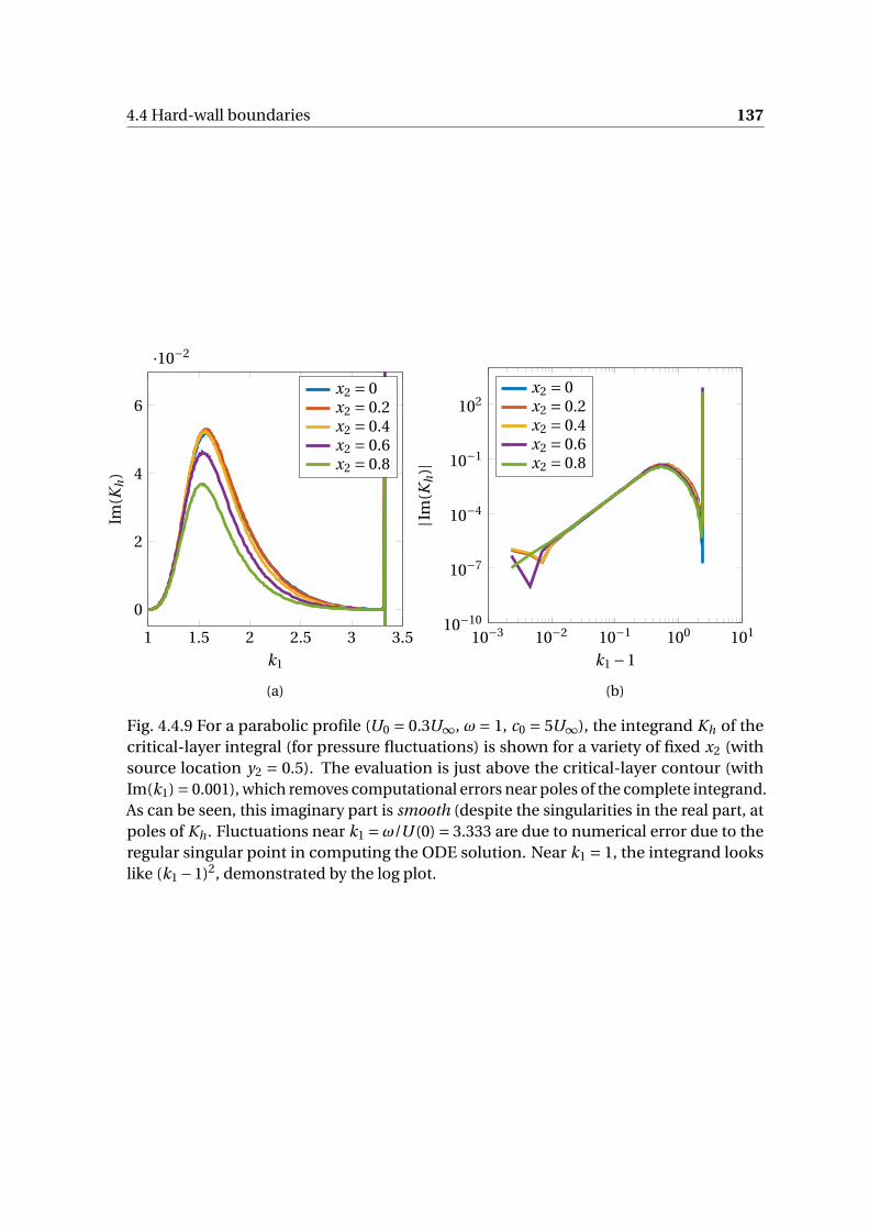
4.4 Hard-wall boundaries 137

1 1.5 2 2.5 3 3.5

0

2

4

6

·10−2

k1

Im(K

h)

x2 = 0x2 = 0.2x2 = 0.4x2 = 0.6x2 = 0.8

(a)

10−3 10−2 10−1 100 10110−10

10−7

10−4

10−1

102

k1 −1

|Im(K

h)|

x2 = 0x2 = 0.2x2 = 0.4x2 = 0.6x2 = 0.8

(b)

Fig. 4.4.9 For a parabolic profile (U0 = 0.3U∞, ω= 1, c0 = 5U∞), the integrand Kh of thecritical-layer integral (for pressure fluctuations) is shown for a variety of fixed x2 (withsource location y2 = 0.5). The evaluation is just above the critical-layer contour (withIm(k1) = 0.001), which removes computational errors near poles of the complete integrand.As can be seen, this imaginary part is smooth (despite the singularities in the real part, atpoles of Kh . Fluctuations near k1 =ω/U (0) = 3.333 are due to numerical error due to theregular singular point in computing the ODE solution. Near k1 = 1, the integrand lookslike (k1 −1)2, demonstrated by the log plot.

138 Disturbances to continuously sheared flow above a homogeneous boundary

dominate), application of both Watson’s and Jordan’s lemma gives

J (x) ∼β1e i axΓ(1+α1)(i x)−(1+α1) −e i bxΓ(1+α2)β2(−i x)−(1+α2). (4.4.9)

Decay is therefore dominated by the end with smaller α j . If the integrand is otherwise

continuous, the remaining integrand decays, at its slowest, like 1/x and thus any integrable

singularities (−1 <α j < 0) dominate the integral. The integrand decays more strongly that

this at either end, as demonstrated by the earlier figure, with decay like (k1 −ω/U∞)2 near

k1 =ω/U∞. Careful comparison with the numerical solution shows that this end does,

however, dominate (with the other end point contribution decaying even more rapidly in

k1) and thus p ′C L ∼ x1

−3 for the case plotted. This algebraic decay is consistent with earlier

work [22].

That the critical-layer decays algebraically downstream is not a new result, but it is

worth remphasising. Firstly, it decays comparatively slowly compared with any stable

modes, and thus might be important at moderate distances downstream (where there are

no unstable modes). Secondly, there is a clear distinction with the piecewise linear case. In

the earlier case, neutrally stable modes, along where a critical-layer would be, could easily

be identified, which did not decay downstream of the source. For a continuously sheared

profile, however, all critical-layer disturbances decay. This highlights a great danger in

a discontinuity in shear: a δ-function in shear gives rise to propagating solutions that

cannot exist for smoothly varying shear.

4.5 Pressure-release and impedance boundaries

The routines outlined for the hard-wall section generalise in a straightforward manner for

more complicated, linear, boundary conditions applied at x2 = 0, though care must be

taken with the existence of boundary-layer modes, which typically show either exponential

growth or decay, arising as isolated zeros of Dℓ.

The routines set up to analyse the dispersion function and to invert the integral es-

sentially depend only on the boundary conditions through the definition of relevant ℓ1

and ℓ2 (so that ℓ1φ′+ℓ2φ= 0 on x2 = 0). For the wall-normal velocity we imposed ℓh

1 =−C 2

0 = −[i (ω−U (0)k1)

]2 and ℓh2 = −3C0C ′

0 = −3(i (ω−U (0)k1))× (−iU ′(0)k1), implicitly

dividing out a constant c20 . Pressure-release conditions are obtained via ℓp

1 = 0,ℓp2 =−C 3

0

and general impedance conditions are straightforward to synthesis by summing these

coefficients. For impedance Z , ℓZj = iωZℓh

j −C0ℓpj . Fundamentally the routine is un-

4.5 Pressure-release and impedance boundaries 139

changed, aside from the excitation of modal solutions away from the critical-layer, which

must be included separately.

4.5.1 Pressure-release conditions

The two pairs of figures, figures 4.5.1 and figures 4.5.2, both consider disturbances to a

parabolic profile, above a pressure-release wall. With lengths scaled by boundary layer

thickness δ, and all speeds by free-stream velocity U∞, we have slip velocity U0 = 0.3 and

free-stream Mach number M∞ = 0.2, corresponding to (constant) speed of sound c0 = 5.

The dispersion function (and thus the majority of singularities of the Fourier trans-

formed disturbance) are shown in figures 4.5.1 for two frequencies, ω = 1 and ω = 20,

chosen to display two distinct characteristics. The former is linearly unstable, with a

pair of conjugate modes lying on either side of the branch cut (with real part ≈ 1 and

imaginary part ≈ 0.3). Either by including these within the branch cut integration contour,

or by calculating the residue at each zero (and thus at each pole of the integrand), it is

straightforward to include this contribution in the fully computed solution, shown in fig-

ure 4.5.2a, with a disturbance growing exponentially downstream. Conversely, the higher

frequency case ω= 20 is stable (see figure 4.5.2b), with the instability modes subsumed

into the critical-layer, and no such exponentially growing disturbance visible. This is

directly analogous to the linearly sheared, incompressible case, where the behaviour and

stabilisation of conjugate modes could be tracked as the frequency was varied.

In fact, it is straightforward to show that these roots of the compressible dispersion

relation are the same modal solutions as in the incompressible case, and are thus hydro-

dynamic in nature (rather than acoustic). Consider a simple piecewise linear profile, for

example, with U0 = 0.2 and U∞ = 1. Using methods outlined in the previous chapter, this

has a pair of conjugate modes in the long-wavelength limit at k1 = 1.3843±0.3621i . Similar

zero finding can be done with finite speed of sound. If c0 = 5 is constant, so reasonably

high Mach number of 0.2, we have zeros at k1 = 1.3855±0.3607i : there is negligible effect

of finite speed of sound on the location of these modes. Even with a more complicated

boundary-layer profile, for example a parabolic boundary-layer profile with the same slip

and free-stream velocities, we have only small displacement with k1 = 1.2071±0.3413i ,

though the effect of varying the profile is clearly a lot greater than of varying the speed of

sound.

Finally, for the higher-frequency case a series of poles appear near the acoustic branch

cut. Poles of the dispersion function do not in themselves contribute to the solution (since

they correspond only to zeros of the integrand), and will not feature in this discussion.

140 Disturbances to continuously sheared flow above a homogeneous boundary

−5 −4 −3 −2 −1 0 1 2 3 4 5

−2

0

2

Re(k1)

Im(k

1)

(a) ω= 1

−100 −80 −60 −40 −20 0 20 40 60 80 100−60

−40

−20

0

20

40

60

Re(k1)

Im(k

1)

(b) ω= 20

Fig. 4.5.1 Phase plot of dispersion function, Dp , as outlined in the text, for two differentfrequencies, one unstable and one stable. Since the axes are both stretched with ω, theacoustic and critical-layer branch cuts are in the same location on the image in each plot.

4.5 Pressure-release and impedance boundaries 141

−2 0 2 4 6 8 10 12 14 16 18 200

2

4

x1

x 2

(a) ω= 1

−2 0 2 4 6 8 10 12 14 16 18 200

2

4

x1

x 2

(b) ω= 20

Fig. 4.5.2 The pressure perturbation above a pressure-release wall, in an unstable configu-ration. We have the standard parabolic profile (U∞ = δ∞ = 1), with U0 = 0.3, and M∞ = 0.2,and two frequencies, ω= 1 and ω= 20 chosen so that unstable modes exist in the formercase, figure 4.5.2a (but not the latter, figure 4.5.2b), growing exponentially downstream.

142 Disturbances to continuously sheared flow above a homogeneous boundary

Far-field noise

As previously, we can compute the far-field acoustic response through evaluation at a

saddle point. This process is identical to the hard-wall procedure, with suitable replace-

ment of functions, and so is not repeated here. In the long-wavelength case, we expect a

dipole-like directivity in pressure due to the boundary-condition now being imposed on

pressure, which mathematically comes out of the evaluation of IF F since Dp , unlike Dh , is

broadly constant in the limit c0 →∞ at the saddle point location.

A sample of far-field directivities has been computed. Firstly, the speed of sound is

increased while holding frequency constant, increasing only the acoustic wavelength, in

figure 4.5.3, showing a similar lobe-like structure to the hard-wall equivalent (though it is

worth noting the number of lobes is generally reduced in all cases, suggesting a reduction

in interference between the source and the reflection from the wall). Similarly, it is easy to

show the far-field dependence on exact flow profile is small analogously to the hard-wall

case (figure 4.4.7). The effect of varying source location is again investigated, and again

(for higher frequencies than previously) a source close to a wall induces lobe-like far-field

behaviour. Direct comparisons between hard-wall and pressure-release directivities will

be investigated below, through variation of impedance Z from ∞ to 0. This also allows

reinvestigation of the far-field results found in the incompressible case in the previous

chapter, §3.6, where the mathematics of the far-field sound calculation were not clear.

4.5.2 General impedance boundary condition

The impedance case arises from taking the boundary condition

LZ01 = iωZV01 −C0P01. (4.5.1)

Other required functions drop out readily from the previous work, for example we can

write

DZ =LZ01φd = iωDh −C0Dp . (4.5.2)

This allows use of previously computed dispersion functions, if desired. Other than the

loss of symmetry in k1 → k∗1 , the process of determining zeros, numerical inversion and

evaluation of far-field acoustics generalises directly from the preceding cases. As with

the long-wavelength case in §3, we expect some number of zeros of DZ , though the

precise number of these boundary-layer modes depends on the precise setup, as does

their resultant stability.

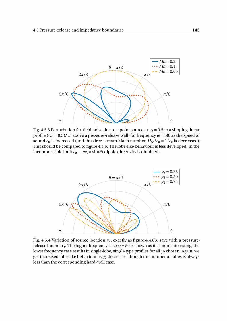
4.5 Pressure-release and impedance boundaries 143

0

π/6

π/3

θ =π/2

π

5π/6

2π/3

Ma = 0.2Ma = 0.1Ma = 0.05

Fig. 4.5.3 Perturbation far-field noise due to a point source at y2 = 0.5 to a slipping linearprofile (U0 = 0.3U∞) above a pressure-release wall, for frequency ω= 50, as the speed ofsound c0 is increased (and thus free-stream Mach number, U∞/c0 = 1/c0 is decreased).This should be compared to figure 4.4.6. The lobe-like behaviour is less developed. In theincompressible limit c0 →∞, a sin(θ) dipole directivity is obtained.

0

π/6

π/3

θ =π/2

π

5π/6

2π/3

y2 = 0.25y2 = 0.50y2 = 0.75

Fig. 4.5.4 Variation of source location y2, exactly as figure 4.4.8b, save with a pressure-release boundary. The higher frequency case ω= 50 is shown as it is more interesting, thelower frequency case results in single-lobe, sin(θ)-type profiles for all y2 chosen. Again, weget increased lobe-like behaviour as y2 decreases, though the number of lobes is alwaysless than the corresponding hard-wall case.

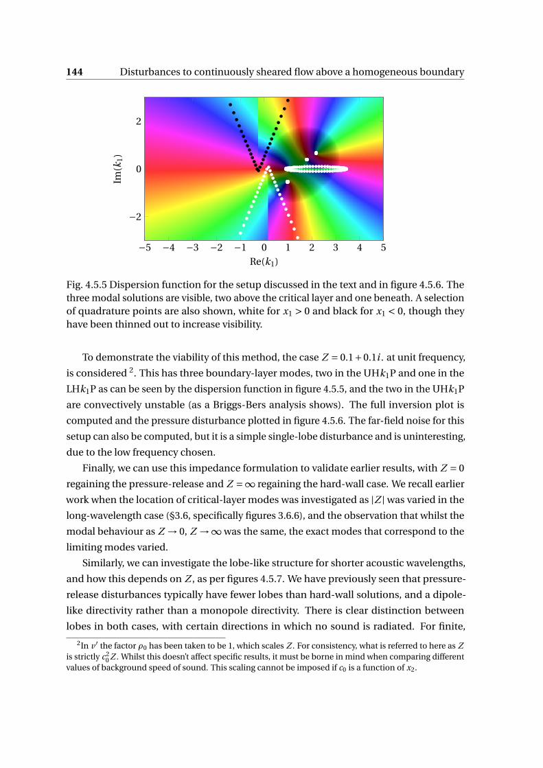
144 Disturbances to continuously sheared flow above a homogeneous boundary

−5 −4 −3 −2 −1 0 1 2 3 4 5

−2

0

2

Re(k1)

Im(k

1)

Fig. 4.5.5 Dispersion function for the setup discussed in the text and in figure 4.5.6. Thethree modal solutions are visible, two above the critical layer and one beneath. A selectionof quadrature points are also shown, white for x1 > 0 and black for x1 < 0, though theyhave been thinned out to increase visibility.

To demonstrate the viability of this method, the case Z = 0.1+0.1i . at unit frequency,

is considered 2. This has three boundary-layer modes, two in the UHk1P and one in the

LHk1P as can be seen by the dispersion function in figure 4.5.5, and the two in the UHk1P

are convectively unstable (as a Briggs-Bers analysis shows). The full inversion plot is

computed and the pressure disturbance plotted in figure 4.5.6. The far-field noise for this

setup can also be computed, but it is a simple single-lobe disturbance and is uninteresting,

due to the low frequency chosen.

Finally, we can use this impedance formulation to validate earlier results, with Z = 0

regaining the pressure-release and Z =∞ regaining the hard-wall case. We recall earlier

work when the location of critical-layer modes was investigated as |Z | was varied in the

long-wavelength case (§3.6, specifically figures 3.6.6), and the observation that whilst the

modal behaviour as Z → 0, Z →∞ was the same, the exact modes that correspond to the

limiting modes varied.

Similarly, we can investigate the lobe-like structure for shorter acoustic wavelengths,

and how this depends on Z , as per figures 4.5.7. We have previously seen that pressure-

release disturbances typically have fewer lobes than hard-wall solutions, and a dipole-

like directivity rather than a monopole directivity. There is clear distinction between

lobes in both cases, with certain directions in which no sound is radiated. For finite,

2In v ′ the factor ρ0 has been taken to be 1, which scales Z . For consistency, what is referred to here as Zis strictly c2

0 Z . Whilst this doesn’t affect specific results, it must be borne in mind when comparing differentvalues of background speed of sound. This scaling cannot be imposed if c0 is a function of x2.

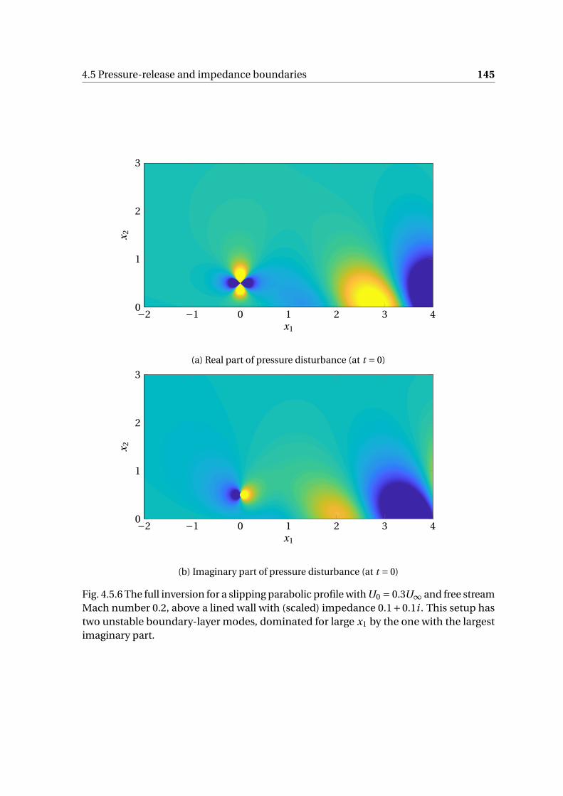
4.5 Pressure-release and impedance boundaries 145

−2 −1 0 1 2 3 40

1

2

3

x1

x 2

(a) Real part of pressure disturbance (at t = 0)

−2 −1 0 1 2 3 40

1

2

3

x1

x 2

(b) Imaginary part of pressure disturbance (at t = 0)

Fig. 4.5.6 The full inversion for a slipping parabolic profile with U0 = 0.3U∞ and free streamMach number 0.2, above a lined wall with (scaled) impedance 0.1+0.1i . This setup hastwo unstable boundary-layer modes, dominated for large x1 by the one with the largestimaginary part.

146 Disturbances to continuously sheared flow above a homogeneous boundary

non-zero Z these lobes are no longer distinct. Whilst there is a clear gradual change

from pressure-release to hard-wall regardless of the sign of Im(Z ), the exact variation

in lobe-like structure is completely different between the two cases. For arg(Z ) = π/4

(figure 4.5.7a), the large pressure-release mode around θ = π/2 quickly splits into two,

with the hard-wall mode with θ slightly larger than 2π/3 quickly forming, even for small

|Z |. The downstream propagating and normal propagating modes are slower to develop.

Conversely, the wall-normal propagating mode develops immediately if arg(Z ) =−π/4

(figure 4.5.7b), centred on θ =π/2, whereas the downstream pressure-release lobe only

slowly separates into two downstream lobes for large |Z |. This observation reinforces what

we have seen before in §3.6: there appears to be no consistent map between Z = 0 and

Z =∞ that can match lobes (or modes) between the two cases.

4.6 Wake solutions

For completeness, the disturbance due to a point source in an unbounded region should

also be considered, relevant to the wake of the trailing-edge of an aerofoil in §6 later. This

has been considered for the the piecewise-linear, long-wavelength case before in §3.7,

though a slightly different approach is considered here due to the limitations of the code

constructed for integration of the governing transformed ODE. The basic setup is shown

in figure 4.6.1.

4.6.1 Auxiliary functions

For the piecewise linear case, we constructed two auxiliary functions to satisfy the bound-

ary conditions, namely decay as x2 →±∞ upon transformation, corresponding to outgo-

ing waves only. This required little extra work, as routines had been constructed to cope

with non-continuous shear, it being the cornerstone of the chapter. However, the code

utilised in this chapter implicitly assumes continuity of U ′ throughout the boundary-layer,

manually taking care of any jump in shear at the edge of the boundary-layer x2 = δ. Most

profiles of interest in the doubly-infinite case have a discontinuity in shear at x2 = 0. With-

out developing methods of integration to cope with this shear jump, it is possible to utilise

earlier code. We describe the background flow profile as

U (x2) =

U+∞ x2 > δ+U+(x2) 0 < x2 < δ+U−(−x2) δ− < x2 < 0

U−∞ x2 < δ−(4.6.1)

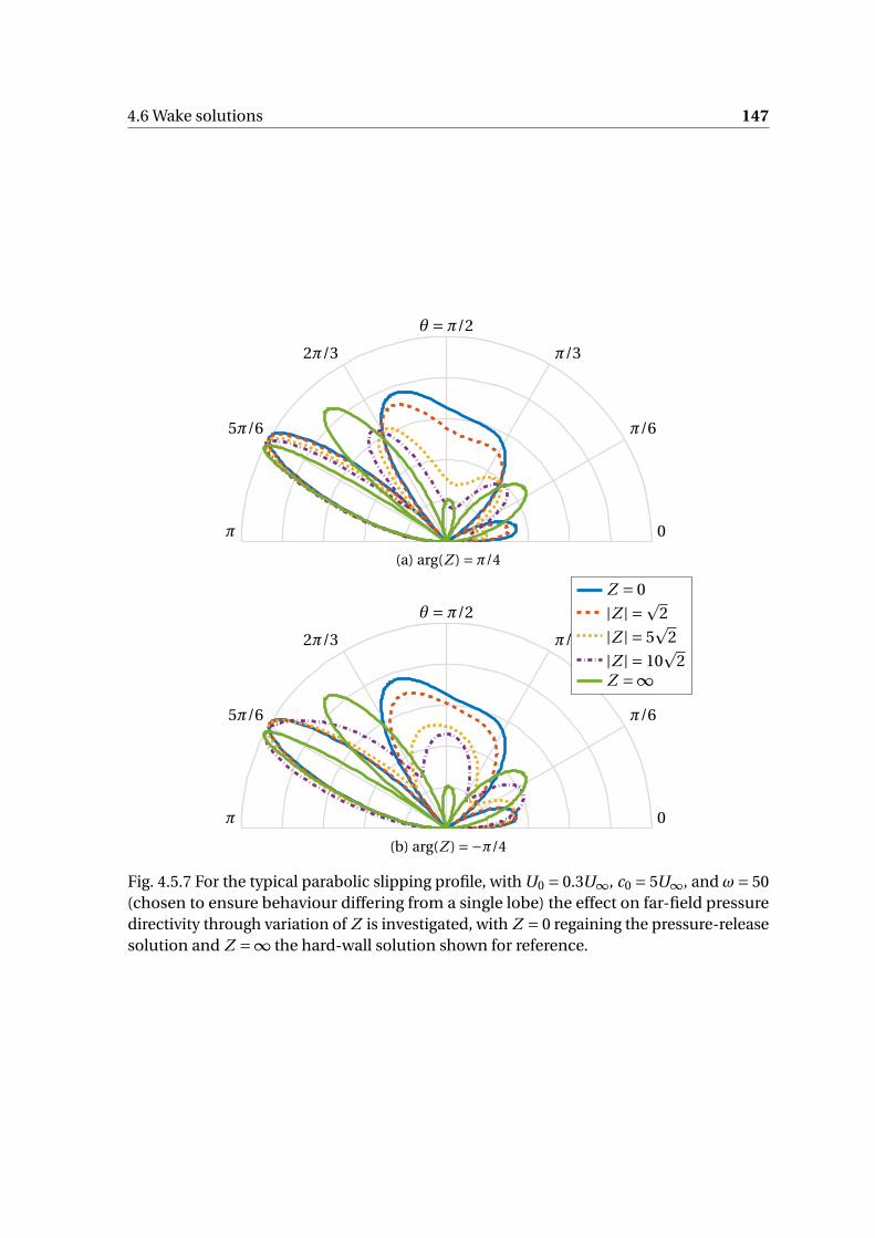
4.6 Wake solutions 147

0

π/6

π/3

θ =π/2

π

5π/6

2π/3

(a) arg(Z ) =π/4

0

π/6

π/3

θ =π/2

π

5π/6

2π/3

Z = 0

|Z | =p2

|Z | = 5p

2

|Z | = 10p

2Z =∞

(b) arg(Z ) =−π/4

Fig. 4.5.7 For the typical parabolic slipping profile, with U0 = 0.3U∞, c0 = 5U∞, and ω= 50(chosen to ensure behaviour differing from a single lobe) the effect on far-field pressuredirectivity through variation of Z is investigated, with Z = 0 regaining the pressure-releasesolution and Z =∞ the hard-wall solution shown for reference.

148 Disturbances to continuously sheared flow above a homogeneous boundary

x2 = δ+

x2 = 0

x2 = δ−

U =U−∞

U =U−(−x2)

U =U0

U =U+(x2)

U =U+∞

q0 y2

Fig. 4.6.1 Setup: a point source above a wake. There is a finite region of shear for δ− < x2 <δ+, potentially with a discontinuity in shear at x2 = 0 (and x2 = δ±. As before, we place apoint mass source at (x1, x2) = (0, y2), assuming y2 > x2.

with δ− < 0 < δ+, and U± both defined for positive arguments z ∈ (0,δ±) respectively.

We can then define decaying auxiliary functions on these half-profiles, as before, with

φ±d (z) the decaying auxlliary function for profile U±(z). The need now is to extend the

φd (−x2), which takes negative values of x2, into the region 0 < x2 < y2, to construct what

has hitherto been referred to as φℓ. We can do this via the imposition

V0+01φℓ(0+) =V0−

01φ−d (0−) (4.6.2a)

P0+01φℓ(0+) =P0−

01φ−d (0−), (4.6.2b)

which is simply continuity of pressure and of vertical velocity across the wake, and takes

into account the jump in shear in the difference between the pressure operators V0± . We

can now essentially think of φℓ as the inner auxiliary function with boundary conditions

on x2 = 0 of the form ℓ1φ′ℓ+ℓ2φ= 0, exactly as before. These functions ℓ j are driven by

the flow beneath the plate, but reduce to routines already used throughout this chapter.

Explicit determination of ℓ1 and ℓ2 is required. Writing V0± = ℓh±1 d/dx2 +ℓh±

2 , and

similarly P0± =±ℓp±1 d/dx2 +±ℓp±

2 we have the linear system

ℓh+1 φ′

ℓ+ℓh+2 φℓ = ℓh−

1 φ−′d +ℓh−

2 φ−d (4.6.3a)

ℓp+1 φ′

ℓ+ℓp+2 φℓ = ℓp−

1 φ−′d +ℓp−

2 φ−d . (4.6.3b)

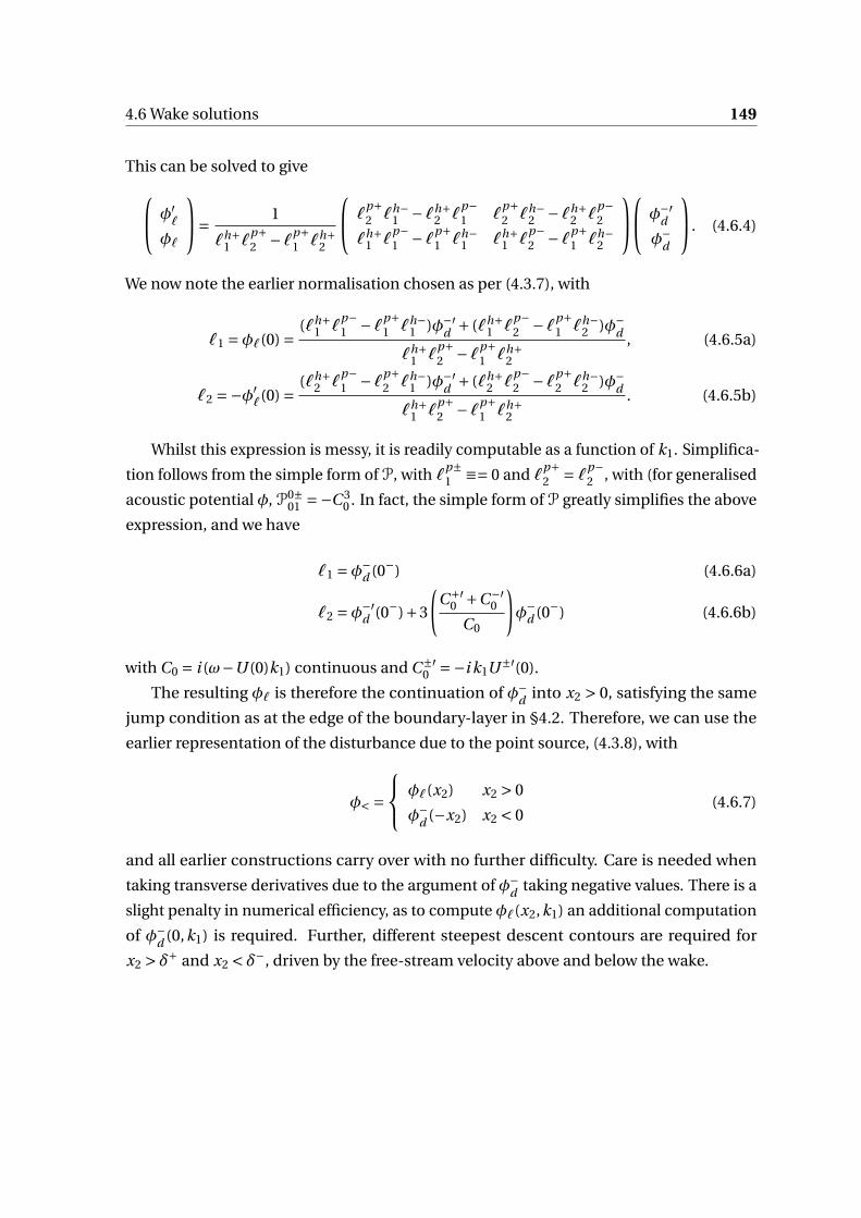
4.6 Wake solutions 149

This can be solved to give φ′ℓ

φℓ

= 1

ℓh+1 ℓ

p+2 −ℓp+

1 ℓh+2

ℓp+2 ℓh−

1 −ℓh+2 ℓ

p−1 ℓ

p+2 ℓh−

2 −ℓh+2 ℓ

p−2

ℓh+1 ℓ

p−1 −ℓp+

1 ℓh−1 ℓh+

1 ℓp−2 −ℓp+

1 ℓh−2

φ−′d

φ−d

. (4.6.4)

We now note the earlier normalisation chosen as per (4.3.7), with

ℓ1 =φℓ(0) = (ℓh+1 ℓ

p−1 −ℓp+

1 ℓh−1 )φ−′

d + (ℓh+1 ℓ

p−2 −ℓp+

1 ℓh−2 )φ−

d

ℓh+1 ℓ

p+2 −ℓp+

1 ℓh+2

, (4.6.5a)

ℓ2 =−φ′ℓ(0) = (ℓh+

2 ℓp−1 −ℓp+

2 ℓh−1 )φ−′

d + (ℓh+2 ℓ

p−2 −ℓp+

2 ℓh−2 )φ−

d

ℓh+1 ℓ

p+2 −ℓp+

1 ℓh+2

. (4.6.5b)

Whilst this expression is messy, it is readily computable as a function of k1. Simplifica-

tion follows from the simple form of P, with ℓp±1 ≡= 0 and ℓp+

2 = ℓp−2 , with (for generalised

acoustic potential φ, P0±01 =−C 3

0 . In fact, the simple form of P greatly simplifies the above

expression, and we have

ℓ1 =φ−d (0−) (4.6.6a)

ℓ2 =φ−′d (0−)+3

(C+′

0 +C−′0

C0

)φ−

d (0−) (4.6.6b)

with C0 = i (ω−U (0)k1) continuous and C±′0 =−i k1U±′(0).

The resulting φℓ is therefore the continuation of φ−d into x2 > 0, satisfying the same

jump condition as at the edge of the boundary-layer in §4.2. Therefore, we can use the

earlier representation of the disturbance due to the point source, (4.3.8), with

φ< = φℓ(x2) x2 > 0

φ−d (−x2) x2 < 0

(4.6.7)

and all earlier constructions carry over with no further difficulty. Care is needed when

taking transverse derivatives due to the argument of φ−d taking negative values. There is a

slight penalty in numerical efficiency, as to compute φℓ(x2,k1) an additional computation

of φ−d (0,k1) is required. Further, different steepest descent contours are required for

x2 > δ+ and x2 < δ−, driven by the free-stream velocity above and below the wake.

150 Disturbances to continuously sheared flow above a homogeneous boundary

4.6.2 Complete inversion

As a specific example for complete inversion, we consider the following group of back-

ground profiles. We define U1(x2) to be a slipping parabolic profile with vanishing shear at

the edge of the boundary layer, x2 = δ= 1 (defining the length scale), with U (0) =U0 = 0.3

and U (δ) =U∞ = 1 (thereby providing the velocity scaling). Similarly, define U2 to be the

parabolic profile with the same slip velocity and boundary-layer thickness and free-stream

velocity 0.5. We can then consider three cases: firstly that both U± =U1, so that the flow

profile is symmetric in x2 7→ −x2, or that U+ =U1 and U− =U2 or vice versa.

0 2 4

−2

0

2

Re(k1)

Im(k

1)

(a) U+ =U− =U1

0 2 4

−2

0

2

Re(k1)

Im(k

1)

(b) U+ =U2, U− =U1 (or vice versa)

Fig. 4.6.2 For ω = 1 and c0 = 5, the wake dispersion functions for the symmetric andasymmetric cases is plotted, as discussed in the text.

In both cases, the profile is unstable at ω= 1, with strong inflection at x2 = 0 driving

this instability. The dispersion functions are shown in figure 4.6.2, for the symmetric and

asymmetric cases (the latter independent of which of U± is U (1,2)). A variety of features of

these functions should be identified, firstly noting the conjugate zeros nearω/U∞ = 1 away

from the real axis, corresponding to an unstable and a stable mode. In the asymmetric

case, these are drawn back towards ω/U2∞ = 2, but still lie in the same broad region of the

complex plane. They grow faster in the asymmetric case, with larger imaginary part.

The dispersion function also has points of note near both types of branch cuts. An

additional branch point exists at ω/U2∞ = 2 in the asymmetric case, though as it lies on

the critical-layer between ω/U1∞ and ω/U0 it is not easy to see. Essentially, we have two

superimposed branch cuts lying along the critical-layer branch cut for x2 ≷ 0 separately.

4.6 Wake solutions 151

This does not occur in the symmetric case when both critical-layer branch cuts lie in the

same place. Lastly, and hard to make out on the given plots, the acoustic branch cuts

divide into two in the asymmetric case: the one driven by the cuts of γ with U =U1(δ+),

and the one driven by cuts of γ with U2(δ−). If these substantially differ, care is required

that the steepest descent contours, which loop their appropriate acoustic branch cut, do

not cross the “new” acoustic branch cut from the flow on the other side of the wake. For

low Mach number flow this is not an issue, as the cuts lie very close to each other, but it

might be an issue at higher Mach numbers with greatly differing flow speeds.

Finally, in the symmetric case we note that, as with the long-wavelength case, we can

relate this dispersion function Dℓ to the product DhDp for the flow profile restricted to

x2 > 0, and thus any hard-wall or pressure-release modes naturally arise as wake modes.

Inversion, up to the caveat that the inversion contour should not cross any additional

acoustic branch cuts, then proceeds as throughout in this chapter. There may be benefits

from using different contours for the branch cut inversion depending on whether x2 ≷ 0.

For the cases we are considering, the full inversion is computed and displayed across

figures 4.6.3 and 4.6.4, picking up modal contributions from the dispersion zeros identified

in figures 4.6.2. The source is always placed at y2 > 0, in the upper flow. The strength of

the source is clearly reduced when the upper flow is slower, even with amplification by the

factor 1/U (y2), which is directly related to the reduction in shear at the source location.

Notwithstanding this, the increased growth rate of the unstable (Kelvin-Helmholtz)

mode is clear in the asymmetric cases (figures 4.6.3b, 4.6.3c), with downstream develop-

ment of the perturbation barely visible in the symmetric case (figure 4.6.3a. Further, it is

possible to eyeball a physical “location” of the resulting instability (at least in the pressure

plots, figure 4.6.3), with the instability localised on the side of x2 = 0 with the largest

free-stream velocity. Conversely, the growth of the wall-normal velocity perturbation

(figure 4.6.4) is always centred on the shear discontinuity itself, at x2 = 0, and shows more

aggressive growth.

4.6.3 Far-field noise

Far-field noise can be computed as before, driven by the saddle point contribution. As

noted, however, the steepest descent contour is a function of the free-stream velocity, and

therefore differs for x2 ≷ 0 if we have an asymmetrical wake, which extends to the location

of the saddle point too. This leads to interesting lobe-like behaviour of the far-field noise

of an asymmetric wake.

Initially, however, it is worth focusing on a symmetric wake, or at least a wake with

U−∞ =U+∞, though the structure of the shear-layer may differ for x2 ≷ 0. This is done in

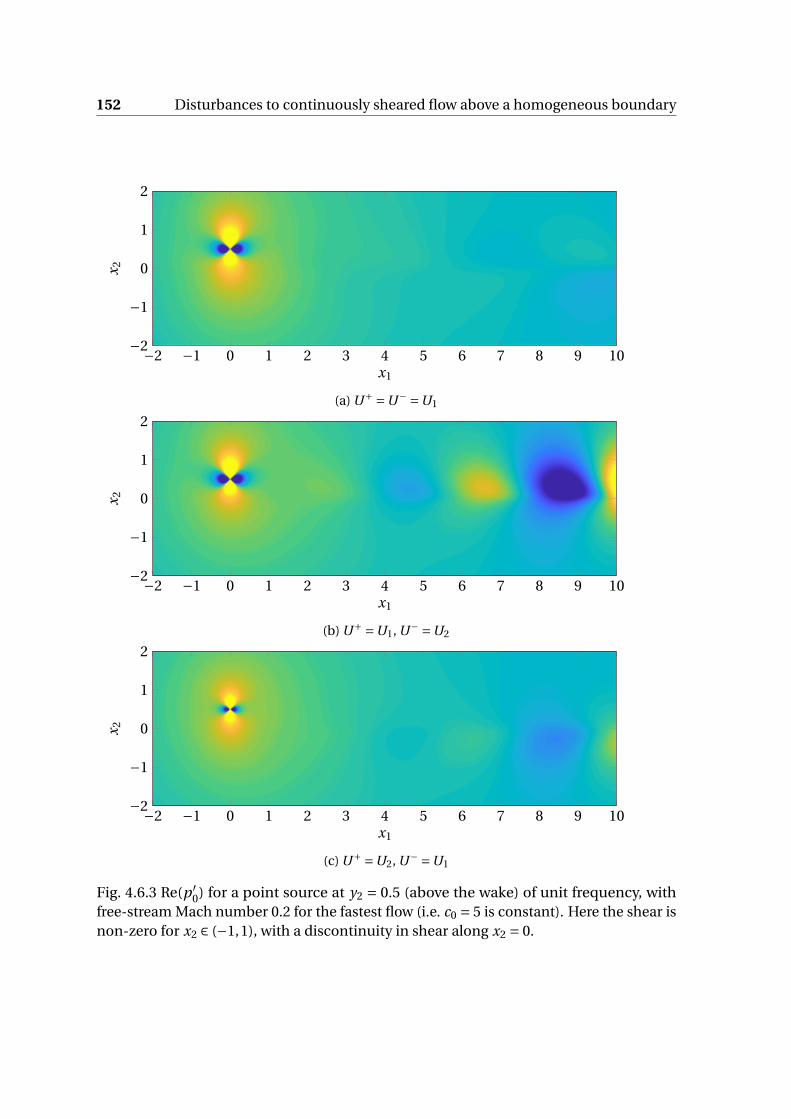
152 Disturbances to continuously sheared flow above a homogeneous boundary

−2 −1 0 1 2 3 4 5 6 7 8 9 10−2

−1

0

1

2

x1

x 2

(a) U+ =U− =U1

−2 −1 0 1 2 3 4 5 6 7 8 9 10−2

−1

0

1

2

x1

x 2

(b) U+ =U1, U− =U2

−2 −1 0 1 2 3 4 5 6 7 8 9 10−2

−1

0

1

2

x1

x 2

(c) U+ =U2, U− =U1

Fig. 4.6.3 Re(p ′0) for a point source at y2 = 0.5 (above the wake) of unit frequency, with

free-stream Mach number 0.2 for the fastest flow (i.e. c0 = 5 is constant). Here the shear isnon-zero for x2 ∈ (−1,1), with a discontinuity in shear along x2 = 0.

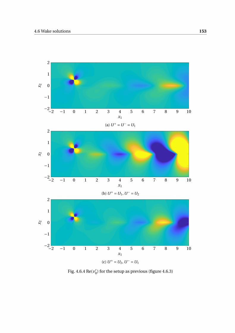
4.6 Wake solutions 153

−2 −1 0 1 2 3 4 5 6 7 8 9 10−2

−1

0

1

2

x1

x 2

(a) U+ =U− =U1

−2 −1 0 1 2 3 4 5 6 7 8 9 10−2

−1

0

1

2

x1

x 2

(b) U+ =U1, U− =U2

−2 −1 0 1 2 3 4 5 6 7 8 9 10−2

−1

0

1

2

x1

x 2

(c) U+ =U2, U− =U1

Fig. 4.6.4 Re(v ′0) for the setup as previous (figure 4.6.3)

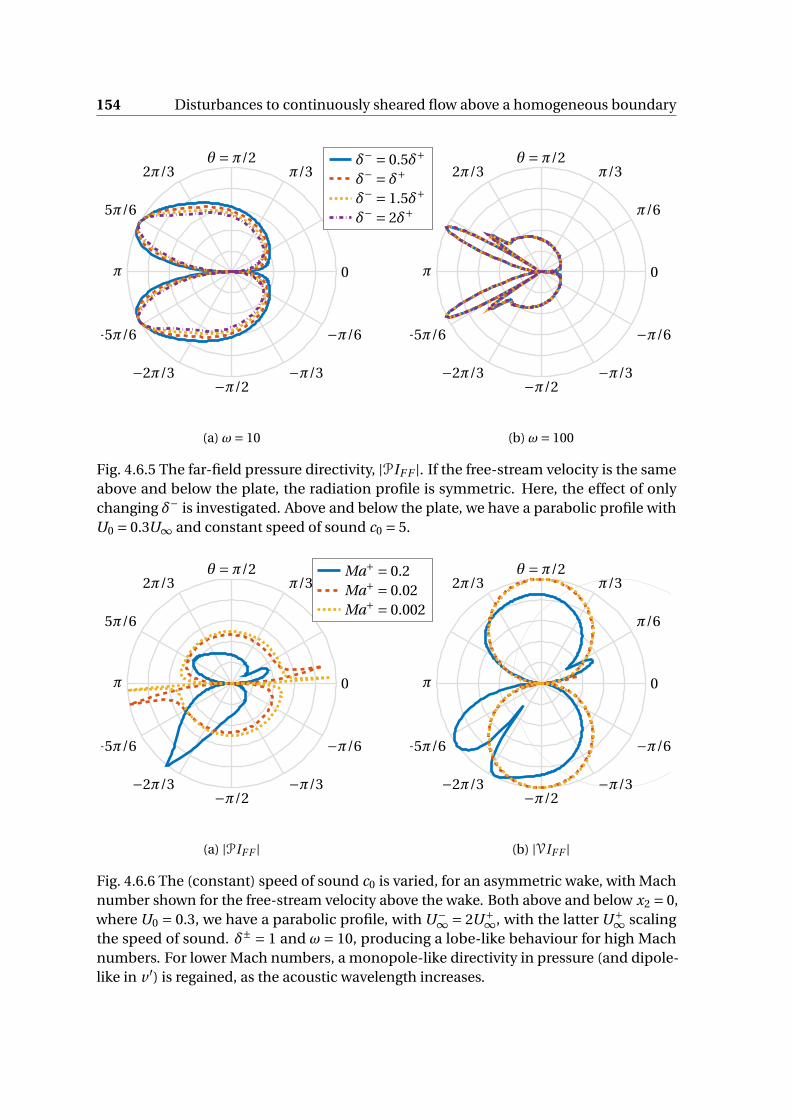
154 Disturbances to continuously sheared flow above a homogeneous boundary

0

π/6

π/3θ =π/2

π

5π/6

2π/3

−π/6

−π/3−π/2

−5π/6

−2π/3

δ− = 0.5δ+

δ− = δ+δ− = 1.5δ+

δ− = 2δ+

(a) ω= 10

0

π/6

π/3θ =π/2

π

2π/3

−π/6

−π/3−π/2

−5π/6

−2π/3

(b) ω= 100

Fig. 4.6.5 The far-field pressure directivity, |PIF F |. If the free-stream velocity is the sameabove and below the plate, the radiation profile is symmetric. Here, the effect of onlychanging δ− is investigated. Above and below the plate, we have a parabolic profile withU0 = 0.3U∞ and constant speed of sound c0 = 5.

0

π/3θ =π/2

π

5π/6

2π/3

−π/6

−π/3−π/2

−5π/6

−2π/3

Ma+ = 0.2Ma+ = 0.02Ma+ = 0.002

(a) |PIF F |

0

π/6

π/3θ =π/2

π

2π/3

−π/6

−π/3−π/2

−5π/6

−2π/3

(b) |VIF F |

Fig. 4.6.6 The (constant) speed of sound c0 is varied, for an asymmetric wake, with Machnumber shown for the free-stream velocity above the wake. Both above and below x2 = 0,where U0 = 0.3, we have a parabolic profile, with U−∞ = 2U+∞, with the latter U+∞ scalingthe speed of sound. δ± = 1 and ω= 10, producing a lobe-like behaviour for high Machnumbers. For lower Mach numbers, a monopole-like directivity in pressure (and dipole-like in v ′) is regained, as the acoustic wavelength increases.

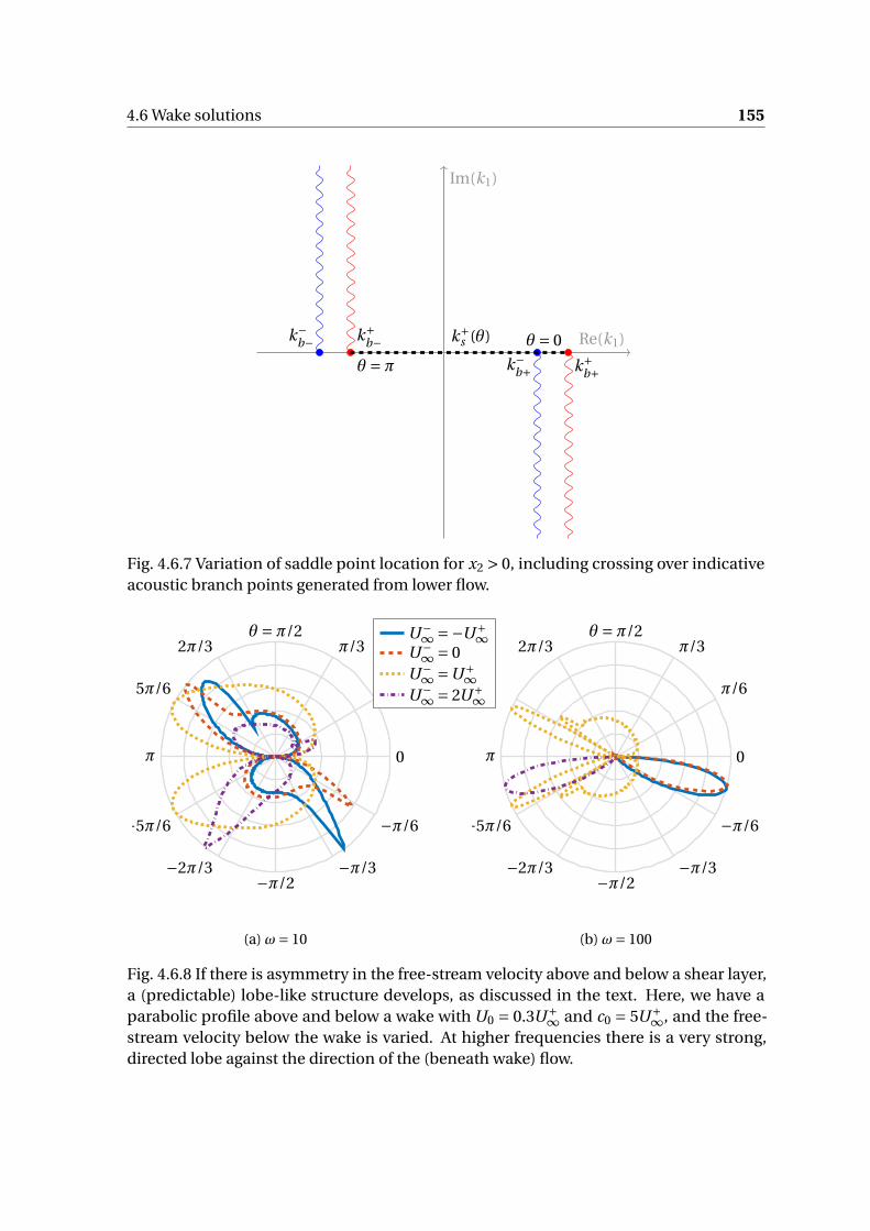
4.6 Wake solutions 155

Re(k1)

Im(k1)

k−b−

k−b+

k+b−

k+b+θ =π

k+s (θ) θ = 0

Fig. 4.6.7 Variation of saddle point location for x2 > 0, including crossing over indicativeacoustic branch points generated from lower flow.

0

π/6

π/3θ =π/2

π

5π/6

2π/3

−π/6

−π/3−π/2

−5π/6

−2π/3

U−∞ =−U+∞U−∞ = 0U−∞ =U+∞U−∞ = 2U+∞

(a) ω= 10

0

π/6

π/3θ =π/2

π

2π/3

−π/6

−π/3−π/2

−5π/6

−2π/3

(b) ω= 100

Fig. 4.6.8 If there is asymmetry in the free-stream velocity above and below a shear layer,a (predictable) lobe-like structure develops, as discussed in the text. Here, we have aparabolic profile above and below a wake with U0 = 0.3U+∞ and c0 = 5U+∞, and the free-stream velocity below the wake is varied. At higher frequencies there is a very strong,directed lobe against the direction of the (beneath wake) flow.

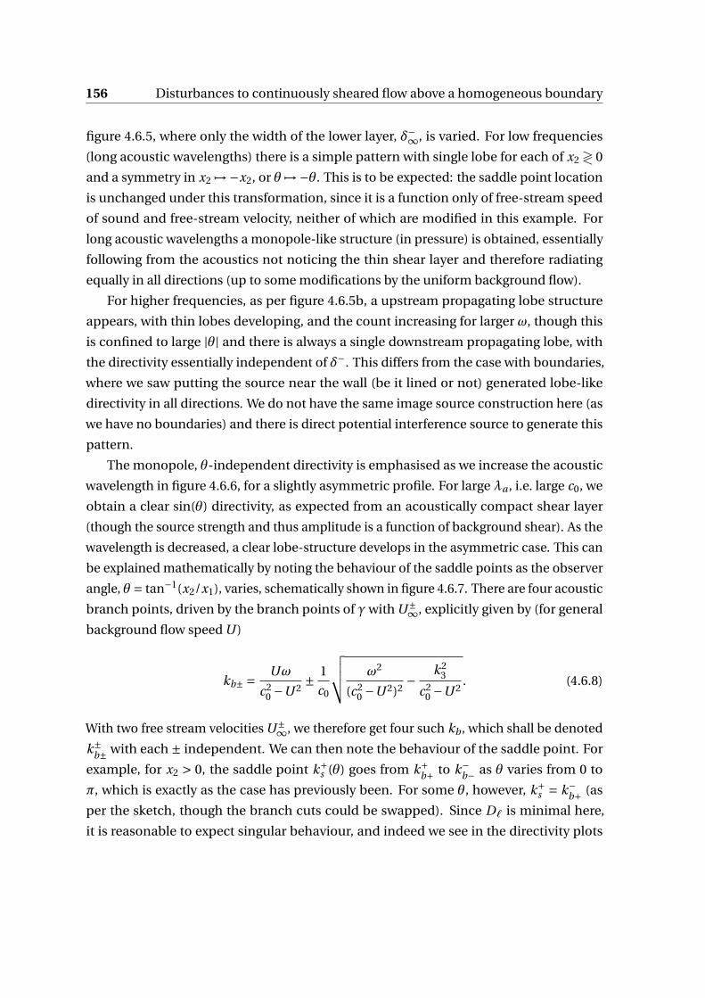
156 Disturbances to continuously sheared flow above a homogeneous boundary

figure 4.6.5, where only the width of the lower layer, δ−∞, is varied. For low frequencies

(long acoustic wavelengths) there is a simple pattern with single lobe for each of x2 ≷ 0

and a symmetry in x2 7→ −x2, or θ 7→ −θ. This is to be expected: the saddle point location

is unchanged under this transformation, since it is a function only of free-stream speed

of sound and free-stream velocity, neither of which are modified in this example. For

long acoustic wavelengths a monopole-like structure (in pressure) is obtained, essentially

following from the acoustics not noticing the thin shear layer and therefore radiating

equally in all directions (up to some modifications by the uniform background flow).

For higher frequencies, as per figure 4.6.5b, a upstream propagating lobe structure

appears, with thin lobes developing, and the count increasing for larger ω, though this

is confined to large |θ| and there is always a single downstream propagating lobe, with

the directivity essentially independent of δ−. This differs from the case with boundaries,

where we saw putting the source near the wall (be it lined or not) generated lobe-like

directivity in all directions. We do not have the same image source construction here (as

we have no boundaries) and there is direct potential interference source to generate this

pattern.

The monopole, θ-independent directivity is emphasised as we increase the acoustic

wavelength in figure 4.6.6, for a slightly asymmetric profile. For large λa , i.e. large c0, we

obtain a clear sin(θ) directivity, as expected from an acoustically compact shear layer

(though the source strength and thus amplitude is a function of background shear). As the

wavelength is decreased, a clear lobe-structure develops in the asymmetric case. This can

be explained mathematically by noting the behaviour of the saddle points as the observer

angle, θ = tan−1(x2/x1), varies, schematically shown in figure 4.6.7. There are four acoustic

branch points, driven by the branch points of γ with U±∞, explicitly given by (for general

background flow speed U )

kb± = Uω

c20 −U 2

± 1

c0

√√√√ ω2

(c20 −U 2)2

− k23

c20 −U 2

. (4.6.8)

With two free stream velocities U±∞, we therefore get four such kb , which shall be denoted

k±b± with each ± independent. We can then note the behaviour of the saddle point. For

example, for x2 > 0, the saddle point k+s (θ) goes from k+

b+ to k−b− as θ varies from 0 to

π, which is exactly as the case has previously been. For some θ, however, k+s = k−

b+ (as

per the sketch, though the branch cuts could be swapped). Since Dℓ is minimal here,

it is reasonable to expect singular behaviour, and indeed we see in the directivity plots

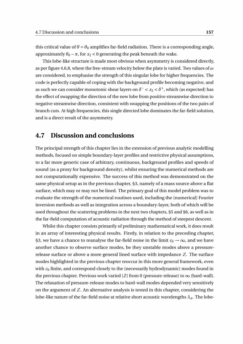
4.7 Discussion and conclusions 157

this critical value of θ = θ0 amplifies far-field radiation. There is a corresponding angle,

approximately θ0 −π, for x2 < 0 generating the peak beneath the wake.

This lobe-like structure is made most obvious when asymmetry is considered directly,

as per figure 4.6.8, where the free-stream velocity below the plate is varied. Two values ofω

are considered, to emphasise the strength of this singular lobe for higher frequencies. The

code is perfectly capable of coping with the background profile becoming negative, and

as such we can consider monotonic shear layers on δ− < x2 < δ+, which (as expected) has

the effect of swapping the direction of the new lobe from positive streamwise direction to

negative streamwise direction, consistent with swapping the positions of the two pairs of

branch cuts. At high frequencies, this single directed lobe dominates the far-field solution,

and is a direct result of the asymmetry.

4.7 Discussion and conclusions

The principal strength of this chapter lies in the extension of previous analytic modelling

methods, focused on simple boundary-layer profiles and restrictive physical assumptions,

to a far more generic case of arbitrary, continuous, background profiles and speeds of

sound (as a proxy for background density), whilst ensuring the numerical methods are

not computationally expensive. The success of this method was demonstrated on the

same physical setup as in the previous chapter, §3, namely of a mass source above a flat

surface, which may or may not be lined. The primary goal of this model problem was to

evaluate the strength of the numerical routines used, including the (numerical) Fourier

inversion methods as well as integration across a boundary-layer, both of which will be

used throughout the scattering problems in the next two chapters, §5 and §6, as well as in

the far-field computation of acoustic radiation through the method of steepest descent.

Whilst this chapter consists primarily of preliminary mathematical work, it does result

in an array of interesting physical results. Firstly, in relation to the preceding chapter,

§3, we have a chance to reanalyse the far-field noise in the limit c0 →∞, and we have

another chance to observe surface modes, be they unstable modes above a pressure-

release surface or above a more general lined surface with impedance Z . The surface

modes highlighted in the previous chapter reoccur in this more general framework, even

with c0 finite, and correspond closely to the (necessarily hydrodynamic) modes found in

the previous chapter. Previous work varied |Z | from 0 (pressure-release) to ∞ (hard-wall).

The relaxation of pressure-release modes to hard-wall modes depended very sensitively

on the argument of Z . An alternative analysis is tested in this chapter, considering the

lobe-like nature of the far-field noise at relative short acoustic wavelengths λa . The lobe-

158 Disturbances to continuously sheared flow above a homogeneous boundary

structure for the pressure-release wall continuously varies as |Z | is increased, limiting to

the hard-wall structure at |Z | =∞, though the precise nature of the lobe decomposition

again depends sensitively on arg(Z ), providing another note of caution in attempting to

match surface modes with pressure-release or hard-wall equivalents.

By allowing finite c0 and short acoustic wavelengths, it is possible to investigate the

much richer far-field noise structure than in the previous chapter. The steepest descent

method explicitly identifies a saddle point lying between the two acoustic branch point,

and numerical methods for finite c0 allow evaluation at exactly this saddle point, unlike

the previous difficulties arising from direct evaluation at k1 = 0 in the incompressible

limit. A noticeable difference arises, however, in the nature of the far-field noise (and,

indeed, the near-field solution) as per §3 and within this chapter. Consider, for example, a

point mass source above a hard-wall. In the limit c0 →∞, this generates an acoustic wave

through the interaction with the background vorticity, which is not the case in this chapter.

For finite, if large, c0, the point mass source generates a pressure wave directly, through

the coupling between perturbation density and pressure through entropy conservation,

regardless of the existence, or not, of background shear. This fundamental difference is

borne out in the both the near-field solution (compare, for example, figures 3.5.5b and

4.4.3a, particularly in the vicinity of the source) and in the far-field directivity. Above a

hard-wall, we have a pressure monopole-like directivity in the large (but finite) c0 limit,

due to constructive interference between the monopole source and its image. Conversely,

there is destructive interference in the infinite c0 case, generating a dipole. For these

reasons, it is difficult to comment on the accuracy of the far-field analysis in the preceding

chapter.

The code and mathematics in this chapter has focused on the assumption of a mono-

tonic, finite, boundary-layer. This assumption of finite boundary-layer not physically

reasonable in practice. For reasonably small Reynolds numbers, we might expect a devel-

oped Blasius-type boundary-layer to have evolved. Whilst this asymptotes to a constant

value as x2 →∞, it does not fit with the finite δ assumption inherent in the numerics.

This is not an insurmountable problem, as the same methods can be developed to in-

clude a boundary-layer profile stretching to x2 →∞, and provides a useful example of a

straightforward extension to the current work. This is not the only limitation as presented

here. Whilst the code as written can cope with both variable c0 (as a proxy for background

density) and spanwise wavenumber k3, the solutions presented in this chapter focus

on the purely two-dimensional case, under the assumption that the Mach number is

sufficiently low that the background speed of sound can be regarded as constant.

Chapter 5

Scattering from a junction

A fundamental problem of acoustics is the generation of sound from the interaction of a

vortical gust solution with a sharp change in boundary conditions. Utilising the Wiener-

Hopf technique, this chapter focuses on the scattering of a hydodynamic disturbance at

an abrupt change to the treatment of a surface, for example the leading- or trailing-edges

of a section of lining. The effect of lining on scattered noise is investigated, including

when a convectively unstable surface mode is excited over a finite region of lining.

5.1 Introduction

So far, we have focused on streamwise homogeneous boundary conditions, more generally

applicable to any problem for which the boundary lies along a streamline of the back-

ground flow, and on which the boundary condition is a function linking φ and ∂φ/∂n

which is independent of position along this streamline. The setup in §3 and §4 permits the

use of the Fourier transform, exploiting the x1-independence of the boundary condition,

which in turn is defined for all x1 ∈ (−∞,∞), with the perturbation being driven by some

point forcing within the body of the fluid.

In many applications we might expect an abrupt change in boundary condition, most

noticeably at the sharp trailing-edge of an aerofoil. This is a well-understood source of

sound, with an efficient conversion of vortical motion to far-field acoustic noise, via the

insistence that the scattered solution is non-singular at the discontinuity itself [31] and

the imposition of the unsteady Kutta condition. Scattering by a sharp trailing-edge is only

one example of the generation of acoustic disturbances by a boundary-layer discontinuity,

and this chapter focuses firstly on the generic junction between two boundary conditions,

before developing the theory to transition between two lined surfaces (or potentially no-

penetration (hard) or pressure-release surfaces), so that there is one boundary condition

160 Scattering from a junction

(along x2 = 0) for x1 < 0 and a different one for x1 > 0. The Wiener-Hopf techinque and

half-range Fourier transforms allow many of the previous methods to transfer to this

problem, which gives great control over the behaviour at the scattering point, without loss

of generality at x1 = x2 = 0.

Scattering by the transition between a hard and soft surface has been considered

previously, though typically in the framework of a duct. In 2007 Rienstra [89] considered

the scattering of a hard-wall duct mode at a hard-soft transition within a duct, identifying

components reflected and transmitted within the duct and drawing parallels with scatter-

ing from the end of a duct. The surface modes previously identified are problematic in this

case, though, with causality analysis difficult in the uniform-flow case, and so a vortex-

sheet type boundary layer (separating zero flow from the mean flow near the boundary)

was considered. More recent work by Singh and Rienstra [93, 101] has considered directly

including a shear layer in the scattering problem with both hard-soft and soft-hard transi-

tions, using the incompressible limit as considered previously by Rienstra and Darau [91].

This formulation raises some questions, both of causality, the direction in which neutrally

stable modes propagate, and in the loss of a cleanly identifiable Wiener-Hopf strip. The

problem therefore requires revisiting as the limit of a well-understood numerical problem,

which is part of what this chapter aims to do.

Via the inclusion of a finite shear layer, the excitation of surface modes is precisely

understood, since they are no longer confined to lie exactly along the wall and instead

propagate within the (now non-infinitesimal) boundary-layer. As well as allowing precise

solution of the scattering problem, this allows discussion of the restabilisation of an

unstable surface mode, for example at the end of a lined section. Downstream of the

lined section we do not expect to find such an unstable mode, which is borne out in the

mathematical analysis. However, if the surface mode is excited for a finite downstream

extent the resulting amplification of the mode can lead to strong acoustic scattering as

it restabilises. Therefore, whilst the surface mode itself might not be a source of sound,

the restabilisation thereof may well be. This is investigated in the limit of acoustically-

decoupled junctions in §5.6.

This chapter begins with an outline of the Wiener-Hopf method and its application to

single-junction scalar problems, for generic differential operators in §5.2. This illustrates

a few technicalities that require care in the Wiener-Hopf process, for example insisting on

continuity of the logarithm along the separation contour, and provides an intuitive repre-

sentation of the Wiener-Hopf kernel as the ratio of upstream and downstream dispersion

functions. This is then applied to the scattering of an incident vortex sheet, from which a

more general gust solution could be constructed (see §6.3) across a hard-soft junction,

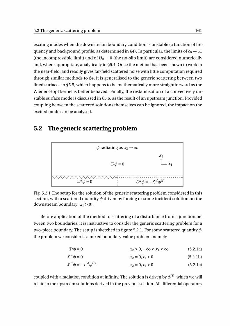
5.2 The generic scattering problem 161

exciting modes when the downstream boundary condition is unstable (a function of fre-

quency and background profile, as determined in §4). In particular, the limits of c0 →∞(the incompressible limit) and of U0 → 0 (the no-slip limit) are considered numerically

and, where appropriate, analytically in §5.4. Once the method has been shown to work in

the near-field, and readily gives far-field scattered noise with little computation required

through similar methods to §4, it is generalised to the generic scattering between two

lined surfaces in §5.5, which happens to be mathematically more straightforward as the

Wiener-Hopf kernel is better behaved. Finally, the restabilisation of a convectively un-

stable surface mode is discussed in §5.6, as the result of an upstream junction. Provided

coupling between the scattered solutions themselves can be ignored, the impact on the

excited mode can be analysed.

5.2 The generic scattering problem

x2

x1Dφ= 0

Luφ= 0 Ldφ=−Ldφ(i )

φ radiating as x2 →∞

Fig. 5.2.1 The setup for the solution of the generic scattering problem considered in thissection, with a scattered quantity φ driven by forcing or some incident solution on thedownstream boundary (x1 > 0).

Before application of the method to scattering of a disturbance from a junction be-

tween two boundaries, it is instructive to consider the generic scattering problem for a

two-piece boundary. The setup is sketched in figure 5.2.1. For some scattered quantity φ,

the problem we consider is a mixed boundary-value problem, namely

Dφ= 0 x2 > 0,−∞< x1 <∞ (5.2.1a)

Luφ= 0 x2 = 0,x1 < 0 (5.2.1b)

Ldφ=−Ldφ(i ) x2 = 0,x1 > 0 (5.2.1c)

coupled with a radiation condition at infinity. The solution is driven by φ(i ), which we will

relate to the upstream solutions derived in the previous section. All differential operators,

162 Scattering from a junction

D, and Lu,d , are linear and independent of the coordinate x1 (which will continue to be

referred to as the streamwise coordinate even for this more general problem), though they

main contain streamwise derivatives ∂/∂x1.

5.2.1 Half-range Fourier transforms and the Wiener-Hopf method

We can solve this problem, provided the integrals converge, using half-range Fourier trans-

forms and applying the Wiener-Hopf method. Given the mixed nature of the boundary

conditions, it is natural to introduce half-range Fourier transforms, defined as

f +1 (k1, x2, t ) =

∫ ∞

0f (x, t )e+i k1x1 dx1, (5.2.2a)

f −1 (k1, x2, t ) =

∫ 0

−∞f (x, t )e+i k1x1 dx1, (5.2.2b)

which together sum to give the full Fourier transform. They behave similarly to Laplace

transformations and can be inverted by considering an inversion contour passing above

or below all singularities as appropriate. Further, they have the property that f +1 is analytic

in the upper-half complex k1 plane (UHk1P) and f −1 in the lower-half complex k1 plane

(LHk1P), a fact that will be exploited in later analysis.

Using these transformations on the boundary condition along x2 = 0 allows recasting

of the problem in k1-space, with as before subscript 1 denoting the streamwise transform

of a quantity and ± (either sub- or superscript) denoting the domain of analyticity of the

function. In Fourier space, (5.2.1) becomes

D1φ1 = 0 x2 > 0 (5.2.3a)

Lu1φ

+1 +pu(k1) = 0 x2 = 0 (5.2.3b)

Ld1φ

−1 +pd (k1) =−Ld

1φ(i )+1 ≡−I+ x2 = 0 (5.2.3c)

The functions pu and pd are end-point contributions, from the truncation of the Fourier

transform. Analogously to the Laplace transform, we have(∂n f

∂xn1

)±1

= (−i k1)n f ±1 ∓

n∑j=1

(−i k1)n− j ∂j−1 f

∂x j−11

(x1 = 0±) (5.2.4)

with the contributions from x1 = 0± (in real space) contributing to the half-range transfor-

mation, though have no impact on analyticity (as polynomials are entire), and they cancel

5.2 The generic scattering problem 163

out in the analysis that follows. This allows definition of the transforms of the operators

Lu,d1 by the substitution ∂/∂x1 =−i k1.

We now have a ordinary differential equation for φ1, with a radiation condition at

infinity. With the chosen convention for temporal Fourier transforms, this becomes a

decay condition as x2 →∞ in k1 space. Denoting the decaying solution of D1φ1 = 0 as φd ,

we have

φ1 = A(k1)φd (5.2.5)

with A to be determined from the boundary conditions. Critically, this means

Lu,d1 φ1 = A(k1)Lu,d

1 φd (5.2.6)

Using this fact, and splitting1 via Lu,d1 φ1 =Lu,d

1 φ+1 +Lu,d

1 φ−1 (see (5.2.12) below) allows

writing down

ALu1φd =−pu + (Lu

1φ1)+ (5.2.7)

ALd1φd =−pu + (Ld

1φ1)−− I+ (5.2.8)

We define the two unknown functions U+ =(Lu

1φ1

)+and U− =

(Ld

1φ1

)−, analytic in the

upper and lower half-planes respectively. We further define the two dispersion functions,

Du,d = Lu,d1 φd , analogous to the previously defined functions. Finally, we define the

Wiener-Hopf kernel

K = Dd

Du= Ld

1φd

Lu1φd

(5.2.9)

linking together the upstream and downstream solutions. With this, we can eliminate A

to give

K (U+−pd ) = (U−−pu)− I+. (5.2.10)

Since the end-point polynomials are entire functions of k1, this is an equation of the

form

K B+ =C−− I+ (5.2.11)

with B+ and C− unknown, except for their domain of complex analyticity. This is a Wiener-

Hopf equation [79], and can be solved for both B+ and C− by appealing to known physical

behaviour of the solution near the boundary discontinuity, or equivalently for large k1. We

suppose, for the time being without proof, that we can decompose any complex analytic

1We assume that the L are (in Fourier space) a polynomial in k1 and therefore entire in k1, so thatLuφ±

1 = (L1φ1

)±.

164 Scattering from a junction

function additively:

F = F++F− (5.2.12)

with superscript ± denoting the half-plane of analyticity (UHk1P or LHk1P respectively).

This is unique up to the addition of an entire function to one side of the factorisation (and

the subsequent subtraction from the other component).

We similarly define the multiplicative factorisation of a function as

F = F+F− (5.2.13)

with the splitfunctions F± analytic and non-zero in their respective half-planes. Armed

with this, we recast the Wiener-Hopf equation (5.2.11) into the following form

K+B++(

I+

K−

)+= C−

K−−

(I+

K−

)−. (5.2.14)

We now suppose that K and I are free of singularities in some strip of the complex plane

containing the real axis 2, and as such so are their factorisations. The left-hand side of the

previous equation is analytic in the UHk1P and the right-hand side on the LHk1P, and the

above construction ensures they agree exactly on the this complex strip, an open set in the

complex plane. By analytic continuation, they define components of the same function.

The LHS indicates the function is analytic in the UHk1P and the RHS the LHk1P, so this

function must be entire, analytic on the entirety of the k1 plane. We denote this function

E , and thus can write down B+ and C− in terms of this entire function, namely

B+ =− 1

K+

(I+

K−

)++ E

K+, (5.2.15)

C− = K−

(I+

K−

)−+K−E . (5.2.16)

We can say something about E if slightly more is known, namely the large k1 behaviour

of B+ and C−. If we can bound their growth by some polynomial, we can use this to bound

E . By (the extended form of) Liouville’s theorem, if we can bound E by a polynomial, then

E is a polynomial of at most that order. In the ideal case, we can bound E by a decaying

function and set it to be zero.2A little care is required here when the frequency ω is real, and can be compared to imposition of the

Briggs-Bers criterion earlier. This is discussed in §5.2.3 below.

5.2 The generic scattering problem 165

Applying these principles to the generic Wiener-Hopf equation we derived earlier gives

A =− 1

K+Du

(I+

K−

)++ E

K+Du(5.2.17)

and the solution to the differential equation is thus

φ(x1, x2) = 1

2π

∫F1

− 1

K+

(I+

K−

)++ E

K+

φd (x2;k1)

Due−i k1x1 dk1 (5.2.18)

where F1 is an integration contour that stretches along the strip of analyticity. We can

directly verify that this does, in fact, describe a solution to the differential equation, by

directly applying the boundary conditions. Applying the upstream operator Lu on x2 = 0

gives

Luφ(x1,0) = 1

2π

∫F1

1

K+

(I+

K−

)++ E

K+

Du

Due−i k1x1 dk1 (5.2.19)

with the remaining integrand analytic in the UHk1P. We can thus close the contour, for

x1 < 0, by a semicircle in the UHk1P, with the contribution decaying exponentially and

thus the integral vanishing as required. Similarly, noting DuK+ = Dd /K− allows rewriting

of the integral as

φ= 1

2π

∫F1

−I++K−

(I+

K−

)−+K−E

φd (x2;k1)

Dd (k1)e−i k1x1 dk1 (5.2.20)

and application of the downstream operator when x2 = 0 separates the integrand into a

component analytic in the lower-half plane and the term consisting purely of the inverse

transform of −I+, thereby closing in the lower-half plane (for x1 > 0) directly reproduces

−I , the term forcing the equation, as expected.

5.2.2 Explicit computation of splitfunctions

Both additive and multiplicative factorisations can be computed explicitly via application

of Cauchy’s integral formula, namely

f (a) =∮

C

f (z)

z −adz (5.2.21)

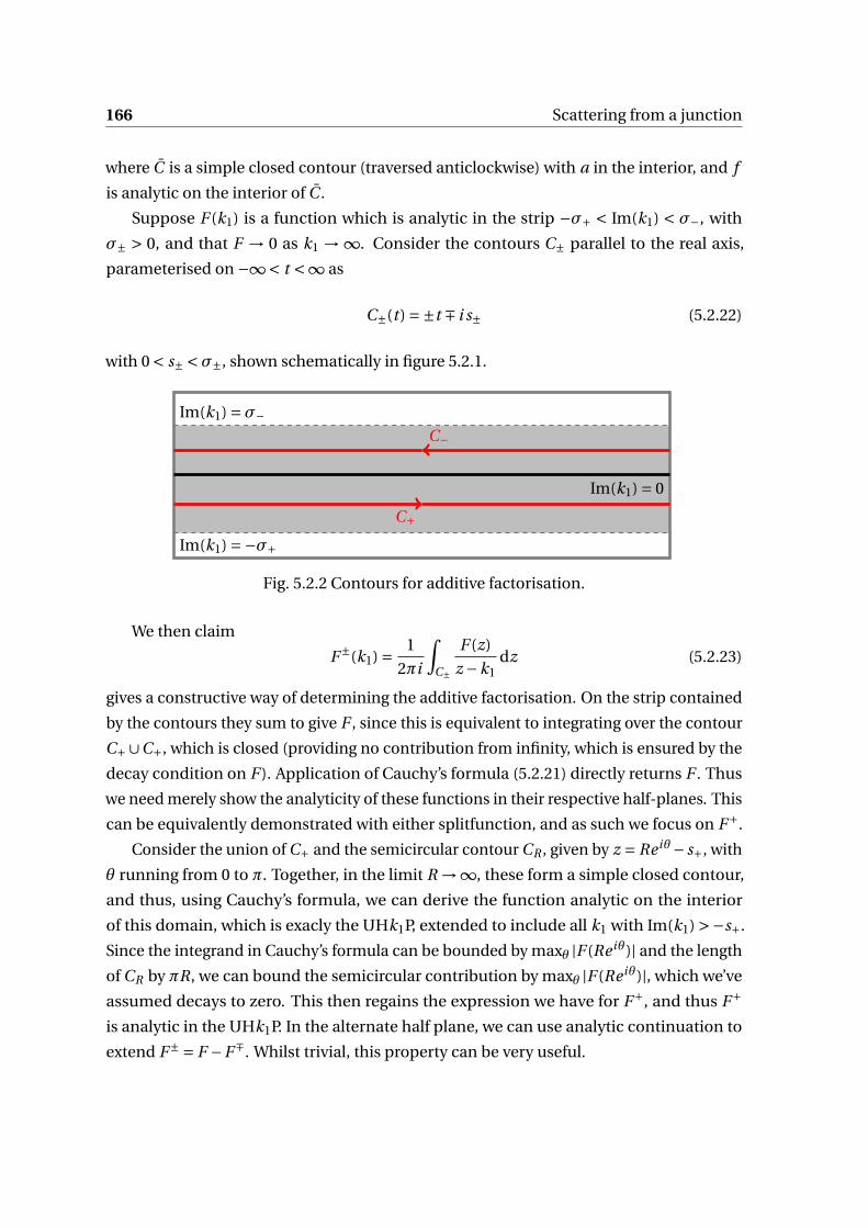
166 Scattering from a junction

where C is a simple closed contour (traversed anticlockwise) with a in the interior, and f

is analytic on the interior of C .

Suppose F (k1) is a function which is analytic in the strip −σ+ < Im(k1) < σ−, with

σ± > 0, and that F → 0 as k1 → ∞. Consider the contours C± parallel to the real axis,

parameterised on −∞< t <∞ as

C±(t ) =±t ∓ i s± (5.2.22)

with 0 < s± <σ±, shown schematically in figure 5.2.1.

Im(k1) =−σ+

Im(k1) =σ−

Im(k1) = 0

C−

C+

Fig. 5.2.2 Contours for additive factorisation.

We then claim

F±(k1) = 1

2πi

∫C±

F (z)

z −k1dz (5.2.23)

gives a constructive way of determining the additive factorisation. On the strip contained

by the contours they sum to give F , since this is equivalent to integrating over the contour

C+∪C+, which is closed (providing no contribution from infinity, which is ensured by the

decay condition on F ). Application of Cauchy’s formula (5.2.21) directly returns F . Thus

we need merely show the analyticity of these functions in their respective half-planes. This

can be equivalently demonstrated with either splitfunction, and as such we focus on F+.

Consider the union of C+ and the semicircular contour CR , given by z = Re iθ− s+, with

θ running from 0 to π. Together, in the limit R →∞, these form a simple closed contour,

and thus, using Cauchy’s formula, we can derive the function analytic on the interior

of this domain, which is exacly the UHk1P, extended to include all k1 with Im(k1) >−s+.

Since the integrand in Cauchy’s formula can be bounded by maxθ |F (Re iθ)| and the length

of CR by πR, we can bound the semicircular contribution by maxθ |F (Re iθ)|, which we’ve

assumed decays to zero. This then regains the expression we have for F+, and thus F+

is analytic in the UHk1P. In the alternate half plane, we can use analytic continuation to

extend F± = F −F∓. Whilst trivial, this property can be very useful.

5.2 The generic scattering problem 167

Formulae for multiplicative factorisation follow directly from additive factorisation. If

F → 1 as k1 →∞, then additive factorisation of log(F ) gives the multiplicative factorisation,

via

log(F+F−) = logF++ logF− = (logF

)++ (logF

)− (5.2.24)

so that F± = exp((logF )±

).

Some functions appear regularly, and it is useful to be able to factorise them efficiently.

A function with a single pole in one half-plane. Consider the function, for some G−

analytic on the LHk1P,

F (k1) = G−(k1)

k1 −kp(5.2.25)

with Im(kp ) < 0. The pole at kp is therefore the only singularity in the LHk1P. This can be

additively factorised on sight to give

F+(k1) = G−(kp )

k1 −kp(5.2.26a)

F−(k1) = G−(k1)−G−(kp )

k1 −kp. (5.2.26b)

Factorisation of γ and |k1|. Consider first the function γ, defined as (compare (4.2.12))

γ2 = k21 +k2

3 − (k0 −Mk1)2 (5.2.27)

with square root branch cuts taken to avoid the real axis when ω has negative imaginary

part. Here, k0 =ω/c0 and M =U /c0 and may both depend on wall-normal coordinate x2.

For fixed x2, we can regard this as a function of k1 with k0 and k3 parameters, writing

γ2 = (1−M 2)k21 +2Mk0k1 +k2

3 −k20

=β2

(k1 − Mk0

β2

)2

−(

k20

β4− k2

3

β2

)=β2

(

k1 − Mk0

β2

)−

√k2

0

β4− k2

3

β2

(k1 − Mk0

β2

)+

√k2

0

β4− k2

3

β2

(5.2.28)

168 Scattering from a junction

with β2 = 1−M 2, and so

γ=β(

k1 − Mk0

β2

)−

√k2

0

β4− k2

3

β2

1/2 (k1 − Mk0

β2

)+

√k2

0

β4− k2

3

β2

1/2

. (5.2.29)

This expression has two branch points, at

k1 = kb± = Mk0

β2±

√k2

0

β4− k2

3

β2(5.2.30)

which unambiguously lie in a complex half-plane when k0 is non-real. So as the resulting

cut of the complex plane does not cross the real axis, these are therefore linked through

infinity when defining the branch cut, provided they lie on either side of the real axis,

which is always the case for subsonic flows (M < 1), real k3 and negative imaginary part of

k0. Provided the square root defining kb± is chosen so that it returns k0/β2 when k3 = 0 (as

opposed to the negative), we have kb± lying in the Lower/Upper Half k1 Plane (L/UHk1P),

respectively. Then defining

γ± =β1/2 (k1 −kb±

)1/2± (5.2.31)

we have exactly that γ= γ+γ− and further that γ± are analytic and nonzero in the U/LHk1P

respectively. We have introduced a new notation for a function

(z − z0)α± (5.2.32)

which (for some complex constant z0) denotes raising complex number (z − z0) to the

non-integral power α, with the branch cut chosen to go from z0 to ∓i∞. If z0 is in the

L/UHzP, this function is analytic in the U/LHzP respectively.

This function is useful for factorising |k1|, which comes up frequently in incompress-

ible applications. For application of the Wiener-Hopf procedure a strip of analyticity

is required, which necessitates regularisation of |k1| (which is analytic nowhere on the

imaginary axis). We define

|k1|ϵ = (k1 + iϵ)1/2+ (k1 − iϵ)1/2

− . (5.2.33)

This regularised function multiplicative factorises into a + and a − function, given by each

bracket in turn, and satisfies |k1|ϵ→|k1| as ϵ→ 0, and so we factorise |k1| as

|k1|± = (k1)1/2± (5.2.34)

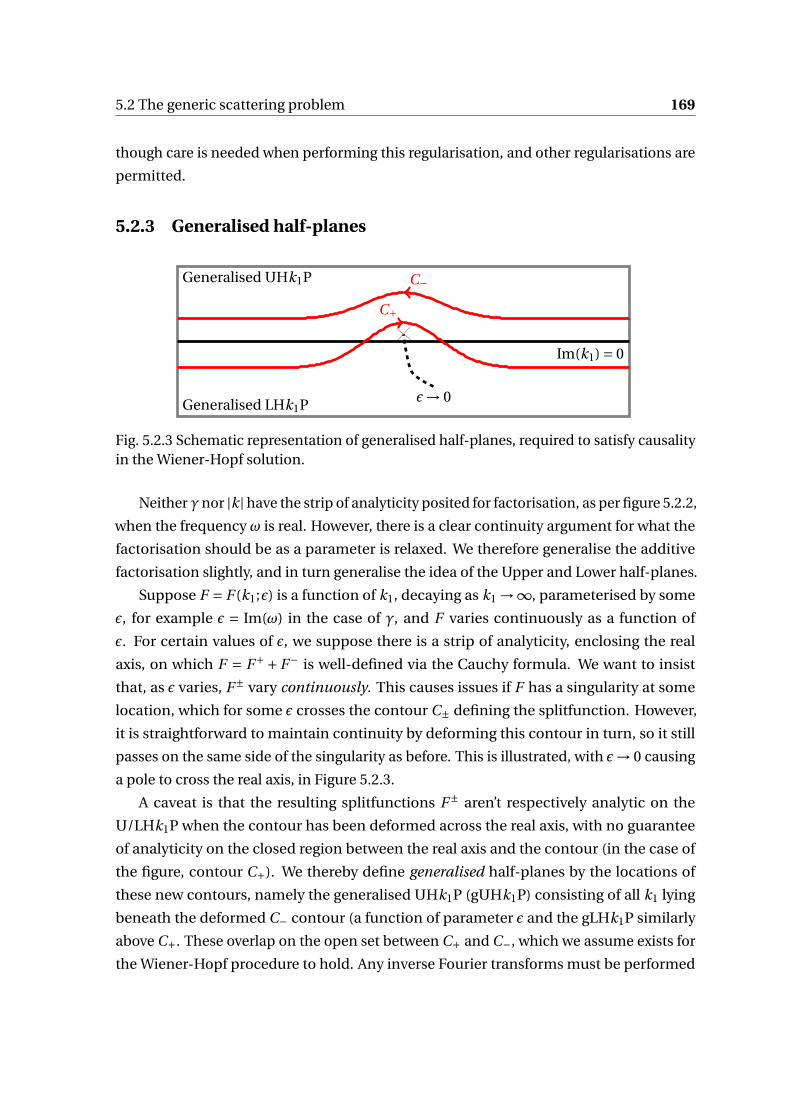
5.2 The generic scattering problem 169

though care is needed when performing this regularisation, and other regularisations are

permitted.

5.2.3 Generalised half-planes

Generalised UHk1P

Generalised LHk1P

Im(k1) = 0

C−

C+

ϵ→ 0

Fig. 5.2.3 Schematic representation of generalised half-planes, required to satisfy causalityin the Wiener-Hopf solution.

Neitherγnor |k|have the strip of analyticity posited for factorisation, as per figure 5.2.2,

when the frequency ω is real. However, there is a clear continuity argument for what the

factorisation should be as a parameter is relaxed. We therefore generalise the additive

factorisation slightly, and in turn generalise the idea of the Upper and Lower half-planes.

Suppose F = F (k1;ϵ) is a function of k1, decaying as k1 →∞, parameterised by some

ϵ, for example ϵ = Im(ω) in the case of γ, and F varies continuously as a function of

ϵ. For certain values of ϵ, we suppose there is a strip of analyticity, enclosing the real

axis, on which F = F++F− is well-defined via the Cauchy formula. We want to insist

that, as ϵ varies, F± vary continuously. This causes issues if F has a singularity at some

location, which for some ϵ crosses the contour C± defining the splitfunction. However,

it is straightforward to maintain continuity by deforming this contour in turn, so it still

passes on the same side of the singularity as before. This is illustrated, with ϵ→ 0 causing

a pole to cross the real axis, in Figure 5.2.3.

A caveat is that the resulting splitfunctions F± aren’t respectively analytic on the

U/LHk1P when the contour has been deformed across the real axis, with no guarantee

of analyticity on the closed region between the real axis and the contour (in the case of

the figure, contour C+). We thereby define generalised half-planes by the locations of

these new contours, namely the generalised UHk1P (gUHk1P) consisting of all k1 lying

beneath the deformed C− contour (a function of parameter ϵ and the gLHk1P similarly

above C+. These overlap on the open set between C+ and C−, which we assume exists for

the Wiener-Hopf procedure to hold. Any inverse Fourier transforms must be performed

170 Scattering from a junction

in this strip of analyticity to preserve causality, and by generalising in this sense we are

essentially using the Briggs-Bers criterion.

5.2.4 Numerical computation of splitfunctions

Consider the Cauchy-type formula for factorisations (5.2.23), generalised to consider C±any (suitable) contour linking −∞ to ∞. This formula will be used repeatedly and it is

useful to have a consistent method of numerical computation of splitfunctions. Suppose

the contour is parameterised as a function of t , running from −∞ to ∞, so that

F± =± 1

2πi

∫ ∞

−∞F (C (t ))

C (t )−k1

dC

dtdt (5.2.35)

where we suppose C (t) → ±∞ as t → ∞. For most of this work, we treat contours of

the form C (t) = t + i f (t), for some f , and so this condition trivially holds provided f is

bounded.

Motivated by Veitch and Peake [109], which were in turn suggested by Rienstra, we

make the substitution 3

t = s

(1− s2). (5.2.36)

Provided F (k1) =O(k−11 ) as k1 →∞, we have the resulting finite integral to determine the

splitfunctions, which can be solved using normal Gaussian quadrature methods (noting

the integrand is finite at the end points of the integration with the decay of F specified),

namely

F± =± 1

2πi

∫ 1

−1

F (C (s/(1− s2)))

C (s/(1− s2))−k1

dC (s/(1− s2))

d(s/(1− s2))

1+ s2

(1− s2)2ds. (5.2.37)

This integral has integration points bunched for smaller k1, which is typically the most

important contribution to the integral, and thus naturally has the behaviour required,

even for a reasonably low number of quadrature points. Examples of using this in practise

are demonstrated in later sections.

5.2.5 Multiplicative factorisation: Winding numbers, continuity of log

and curved branch cuts

An earlier comment noted that, if F → 1 as k1 →∞, then additive factorisation of log(F )

suffices to determine the multiplicative factorisation of F . This is easily illustrated to be

3This differs slightly from the reference text, and is valid for all t , both positive and negative.

5.2 The generic scattering problem 171

an oversimplification, by considering for example

F (z) = z − z+z − z−

(5.2.38)

with z± in the U/LHzP respectively. Whilst this is trivially factorisable, and F → 1 in all

directions, we cannot say that log(F ) → 0 in all directions, due to the change in argument

of the function. If arg(F ) = 0 as z →∞ along the positive real axis, then if we move left-

wards along the real axis we find that arg(F ) = −2π as z →−∞. These two limits only

have log(F ) → 0 if a branch cut of log has been crossed, which invalidates the factorisa-

tion method (which assumes the function, in this case log(F ), is continuous along the

factorisation contour).

The fundamental problem with this function is that the winding number of the func-

tion around 0 is non-zero: there is an overall gain or loss of argument along the separation

contour. If we were to plot F (z) in the complex plane as z varies along the real axis, it would

go from 1 to 1 by making a loop around z = 0. There is therefore no way to determine a

branch cut of log(F ), beginning at 0 and stretching to ∞, such that F (z) does not at some

point cross the cut. This is relatively straightforward to deal with, as suggested by the

example given which can be trivially factorised. We extend this to deal with other cases

[79].

Suppose we only impose that |F | → 1 as z →∞, and is analytic on the real axis (or

whichever contour we choose that asymptotes to the real axis for large z). For some real µ,

ν, we have

F → e iµ z →−∞,

e iν z →+∞.(5.2.39)

Picking two useful branch points (which will depend on the function of choice) z± (in the

U/LHzP), the reduced function F , defined as

F (z) = F (z)e−iµ(z − z−)α+(z − z+)−α− , (5.2.40)

satisfies F → 1 as z →±∞. Here, α is defined as

α= 1

2π

(ν+µ)

. (5.2.41)

As before, the branch cuts of (z)α± are defined to connect 0 and ∓i∞, so that, for exam-

ple, (z − z+)α− is a −-function, analytic in the LHzP. F is then amenable to numerical

factorisation. If F is shown to have non-zero winding number after this analysis, it is

172 Scattering from a junction

straightforward to increase or decrease α by an integer amount. With F factorised, then

F±(z) = e iµ/2F±(z)(z − z∓)±α± (5.2.42)

follows, the leading e iµ/2 chosen for symmetry though as a constant its splitting between

F± is somewhat arbitrary.

This elimination of the nonzero winding number ensures that, provided log is fixed to

be continuous along the factorisation contour, F can be factorised numerically. Construct-

ing such a logarithm is numerically tricky, as some degree of automation determining

whether a branch cut has been crossed is needed. A more readily useable approach is to

use a curved branch cut of log, which is applicable in most circumstances, provided a path

can be found from 0 to ∞ without the complex curve w = F (z) (for z along the separation

contour) being crossed, though we do not need to use this method in this work.

Whilst we have assumed µ and ν are real, this constraint is not necessary and they can

be complex indices. This greatly expands the number of problems that can be directly dealt

with using this method, though issues of boundedness need to be carefully considered

when α is complex. This is first done in §5.4, though appears throughout this chapter and

the following one.

5.2.6 Linking small x1 and large k1 behaviour

Generalising the method of stationary phase, we can relate the near-field physical be-

haviour of a function with its far-field behaviour in Fourier space. For a function f ∼ xα as

x → 0, the resulting half-range transform is dominated near x = 0 as k →∞, with trans-

formed function F (k) ∼ k−(1+α). If we use physical arguments to bound real variables near

a junction (x = 0), then we obtain large k1 bounds on the resulting half-range transforms.

This will in turn provide a bound on the entire function E(k1).

In the presence of mean flow, it is typically possible to impose a Kutta condition [31], by

which we prescribe that (physical) perturbation quantities are finite at the junction x = 0,

and so α> 0 for both velocity and pressure perturbations. As discussed by [31], this is not

necessarily possible to impose if there is no background flow, which naturally arises if we

have a non-slipping profile. In this case, typically finite pressure and (integrably) singular

velocities would be expected, so that α>−1 for the velocity field. Were we to not impose

such conditions, the addition of eigensolutions, singular at the junction, driven by the

value of the entire function E , would contribute to the solution. Alternative considerations

involve insisting the energy generated from the junction is suitably well-defined.

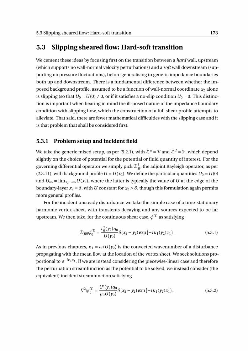
5.3 Slipping sheared flow: Hard-soft transition 173

5.3 Slipping sheared flow: Hard-soft transition

We cement these ideas by focusing first on the transition between a hard wall, upstream

(which supports no wall-normal velocity perturbations) and a soft wall downstream (sup-

porting no pressure fluctuations), before generalising to generic impedance boundaries

both up and downstream. There is a fundamental difference between whether the im-

posed background profile, assumed to be a function of wall-normal coordinate x2 alone

is slipping (so that U0 =U (0) = 0, or if it satisfies a no-slip condition U0 = 0. This distinc-

tion is important when bearing in mind the ill-posed nature of the impedance boundary

condition with slipping flow, which the construction of a full shear profile attempts to

alleviate. That said, there are fewer mathematical difficulties with the slipping case and it

is that problem that shall be considered first.

5.3.1 Problem setup and incident field

We take the generic mixed setup, as per (5.2.1), with Lu =V and Ld =P, which depend

slightly on the choice of potential for the potential or fluid quantity of interest. For the

governing differential operator we simply pick D†R , the adjoint Rayleigh operator, as per

(2.3.11), with background profile U =U (x2). We define the particular quantities U0 =U (0)

and U∞ = limx2→∞U (x2), where the latter is typically the value of U at the edge of the

boundary-layer x2 = δ, with U constant for x2 > δ, though this formulation again permits

more general profiles.

For the incident unsteady disturbance we take the simple case of a time-stationary

harmonic vortex sheet, with transients decaying and any sources expected to be far

upstream. We then take, for the continuous shear case, φ(i ) as satisfying

DR0φ(i )0 = c2

0(y2)q0

U (y2)δ(x2 − y2)exp

(−iκ1(y2)x1)

. (5.3.1)

As in previous chapters, κ1 = ω/U (y2) is the convected wavenumber of a disturbance

propagating with the mean flow at the location of the vortex sheet. We seek solutions pro-

portional to e−iκ1x1 . If we are instead considering the piecewise-linear case and therefore

the perturbation streamfunction as the potential to be solved, we instead consider (the

equivalent) incident streamfunction satisfying

∇2ψ(i )0 = U ′(y2)q0

ρ0U (y2)δ(x2 − y2)exp

(−iκ1(y2)x1)

. (5.3.2)

174 Scattering from a junction

This section will primarily focus on the former, though the intricacies introduced by the

latter will be remarked upon later (primarily with issues of |k1| in the imcompressible

case).

Using earlier notation and computed functions, we write down the solution to (5.3.1),

satisfying the upstream hard-wall boundary condition, as

φ(i )0 = c2

0(y2)q0

U (y2)exp

(−iκ1(y2)x1) φ≷(x2;κ1)φ≶(y2;κ1)

W (y2)(5.3.3)

with φ≷(x2;k1) =φd for x2 > y2 and φh for x2 < y2 (with φ≶ the other of these functions) –

the only difference for more general boundary-conditions is the replacement of φh by the

appropriate solution satisfying the upstream boundary condition. We can then use (4.3.6)

to write this in terms of the hard-wall dispersion function, evaluated at k1 = κ1 =ω/U (y2),

and so

φ(i )0 = c2

0(y2)q0

U (y2)

exp(−iκ1(y2)x1

)Dh(κ1)

c0(y2)2C (y2)4

c0(0)2C (0)4φ≷(x2;κ1)φ≶(y2;κ1) (5.3.4)

Since much of this is a function of y2 alone (either directly or through κ1) and does not

materially effect the scattering problem, we consider the generic incident field

φ(i )0 =Q0(y2)φ≷(x2;κ1)φ≶(y2;κ1)exp

(−iκ1x1)

(5.3.5)

noting that due to linearity the solution is proportional to Q0. There are issues with

evaluating the auxiliary functions at k1 = κ1 due to the critical-layer, and so deformed

contour methods should be utilised as per §4.2.4 to avoid the singularity in the governing

equations, with consistency needed between the direction the contour loops the regular

singular point in calculation of φd , φh and Dh .

The scattered problem, in Fourier-space, is forced by

I+ =(P0φ

(i )0

)+1

. (5.3.6)

Since the only x1 dependence of the incident field is through the oscillatory term

exp(−iκ1x1) and P does not explicitly depend on x1, P0φ(i )0 depends on x1 only through

this oscillatory term. The half-range transform can then be computed as

I+ =Q0(y2)φ≶(y2;κ1)[P01(κ1)φ≷(x2;κ1)

]∫ ∞

0e−iκ1x1 e i k1x1 dx1

=Q0(y2)φd (y2;κ1)[P01(κ1)φh(0;κ1)

] i

(k1 −κ1).

(5.3.7)

5.3 Slipping sheared flow: Hard-soft transition 175

Aside from the single pole in the LHk1P at k1 = κ1, this function is analytic. Note that

this pole lies on the real axis when ω is real, but should be considered as lying in the

(generalised) lower half k1-plane.

5.3.2 The Wiener-Hopf kernel and factorisation

The Wiener-Hopf kernel is given by

K (k1) = Dp (k1)

Dh(k1)(5.3.8)

with zeros at zeros of Dp and poles at zeros of Dh , and a typical pair of acoustic branch

cuts. Numerical formulae for multiplicative factorisation exist from (5.2.21), though these

require a normalised kernel such that K → 1 as k1 →∞, and thus require an understanding

of the large-k1 behaviour of K , which can be obtained from the asymptotic analysis in

§4.2.5, which exactly gives large k1 expressions for φd , from which large k1 expressions for

Pφd and Vφd can easily be derived. We have

Dp ∼−C 3φ (5.3.9a)

Dh ∼ γC 2φ (5.3.9b)

where φ can be computed, but is common to both functions. Both γ and C are evaluated

for U =U0, and importantly are both large as k1 →∞. This is where there is a difference

for the non-slip case, with Dh missing terms that are here smaller in k1, but of equal

importance when U0 = 0 (so that C is O(k01) and is small). The resulting large k1 kernel is

then

K f =−C

γ. (5.3.10)

There are other functions (less physically motivated) that have the same large k1-

behaviour as K , however this choice of K f can be factorised directly from earlier work.

C = i (ω−U0k1) has a single zero in the (generalised) lower half plane, and is thus already

a + function, and γ has previously been factorised in section 5.2, so that

K f + =− C

γ+, (5.3.11a)

K f − = 1

γ−. (5.3.11b)

176 Scattering from a junction

The normalised kernel K = K /K f can then be factorised numerically (with care to ensure

poles and zeros of the kernel are correctly assigned a half-plane), to give K = K+K− and

thus

K± = K±K f ±. (5.3.12)

Whilst the factorisation needs to be done, we can use this expression to determine the large

k1-behaviour of the factorised kernel, which will allow bounding of the entire function

E (k1). We note that factorisation via the Cauchy formula, (5.2.23), implies that if F → 0 as

k1 →∞ then both F± → 0 as k1 →±∞. This convenient choice of factorisation, applied to

log K , implies K± → 1 as k1 →∞, and hence far-field behaviour is determined by far-field

behaviour of K f ,±. This presupposes the condition outlined in §5.2.5 has been satisfied,

that the winding number of K about 0 is 0 and log(K ) can be chosen to be continuous

along the separation contours, with suitable decay at infinity. This can be demonstrated

to be valid under the choice of K f for this slipping case, by plotting log(K ) in the complex

plane along the separation contour, as done later for the no-slip kernel in figure 5.4.1b.

We therefore have

K± ∼ k±1/21 (5.3.13)

as k1 →∞. This allows bounding of the entire function E(k1).

Numerical factorisation of reduced kernel

A generic example of the unreduced Wiener-Hopf kernel K is shown in figure 5.3.1, for a

simple parabolic profile (unstable above a pressure-release wall). It has a similar struc-

ture to previously seen dispersion functions, with zeros at zeros of the pressure-release

dispersion function and branch cuts along the critical layer and acoustic branch cuts cor-

responding to those of γ. Factorisation requires that the (convectively unstable) pressure-

release zeros remain in the generalised lower half-plane, and thus factorisation contours

must be deformed as indicated schematically in figure 5.3.2. It is worth noting the same

factorisation contour can be used for both + and − factorisations, though this removes

the self-checking strip on which K+ = K /K− (and vice versa).

A typical factorisation contour used is a “tanh” contour, with

C (t ) = t + i

a +b tanh

(2

t+− t−

(t − t++ t−

2

)) . (5.3.14)

This gives a contour with imaginary part tending to a ± b as t → ±∞, with t+ and t−controlling the steepness and centre of the contour, and allowing it to be chosen to pass

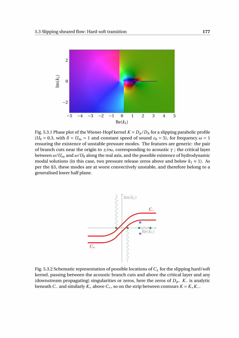
5.3 Slipping sheared flow: Hard-soft transition 177

−5 −4 −3 −2 −1 0 1 2 3 4 5

−2

0

2

Re(k1)

Im(k

1)

Fig. 5.3.1 Phase plot of the Wiener-Hopf kernel K = Dp /Dh for a slipping parabolic profile(U0 = 0.3, with δ = U∞ = 1 and constant speed of sound c0 = 5), for frequency ω = 1ensuring the existence of unstable pressure modes. The features are generic: the pairof branch cuts near the origin to ±i∞, corresponding to acoustic γ ; the critical layerbetween ω/U∞ and ω/U0 along the real axis, and the possible existence of hydrodynamicmodal solutions (in this case, two pressure release zeros above and below k1 ≈ 1). Asper the §3, these modes are at worst convectively unstable, and therefore belong to ageneralised lower half plane.

Re(k1)

Im(k1)

C−

C+

Fig. 5.3.2 Schematic representation of possible locations of C± for the slipping hard/softkernel, passing between the acoustic branch cuts and above the critical layer and any(downstream propagating) singularities or zeros, here the zeros of Dp . K− is analyticbeneath C− and similarly K+ above C+, so on the strip between contours K = K+K−.

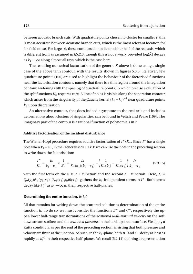
178 Scattering from a junction

between acoustic branch cuts. With quadrature points chosen to cluster for smaller t , this

is most accurate between acoustic branch cuts, which is the most relevant location for

far-field noise. For large |t |, these contours do not lie on either half of the real axis, which

is different from as assumed in §5.2.3, though this is not a worry provided log(K ) decays

as k1 →∞ along almost all rays, which is the case here.

The resulting numerical factorisation of the generic K above is done using a single

case of the above tanh contour, with the results shown in figures 5.3.3. Relatively few

quadrature points (100) are used to highlight the behaviour of the factorised functions

near the factorisation contours, namely that there is a thin region around the integration

contour, widening with the spacing of quadrature points, in which precise evaluation of

the splitfunctions K± requires care. A line of poles is visible along the separation contour,

which arises from the singularity of the Cauchy kernel (k1 −kq )−1 near quadrature points

kq upon discretisation.

An alternative contour, that does indeed asymptote to the real axis and includes

deformations about clusters of singularities, can be found in Veitch and Peake [109]. The

imaginary part of the contour is a rational function of polynomials in t .

Additive factorisation of the incident disturbance

The Wiener-Hopf procedure requires additive factorisation of I+/K−. Since I+ has a single

pole when k1 = κ1, in the (generalised) LHk1P, we can use the note in the preceding section

to write down the factorisation:

I+

K−= I0

k1 −κ1× 1

K−= I0

K−(κ1)(k1 −κ1)+

(1

K−(k1)− 1

K−(κ1)

)I0

k1 −κ1(5.3.15)

with the first term on the RHS a + function and the second a − function. Here, I0 =Q0(y2)φd (y2;κ1)

[P01(κ1)φh(0;κ1)

]gathers the k1-independent terms in I+. Both terms

decay like k−11 as k1 →∞ in their respective half-planes.

Determining the entire function, E(k1)

All that remains for writing down the scattered solution is determination of the entire

function E . To do so, we must consider the functions B+ and C−, respectively the up-

per/lower half-range transformations of the scattered wall-normal velocity on the soft,

downstream surface, and the scattered pressure on the hard, upstream surface. We apply a

Kutta condition, as per the end of the preceding section, insisting that both pressure and

velocity are finite at the junction. As such, in the k1-plane, both B+ and C− decay at least as

rapidly as k−11 in their respective half-planes. We recall (5.2.14) defining a representation

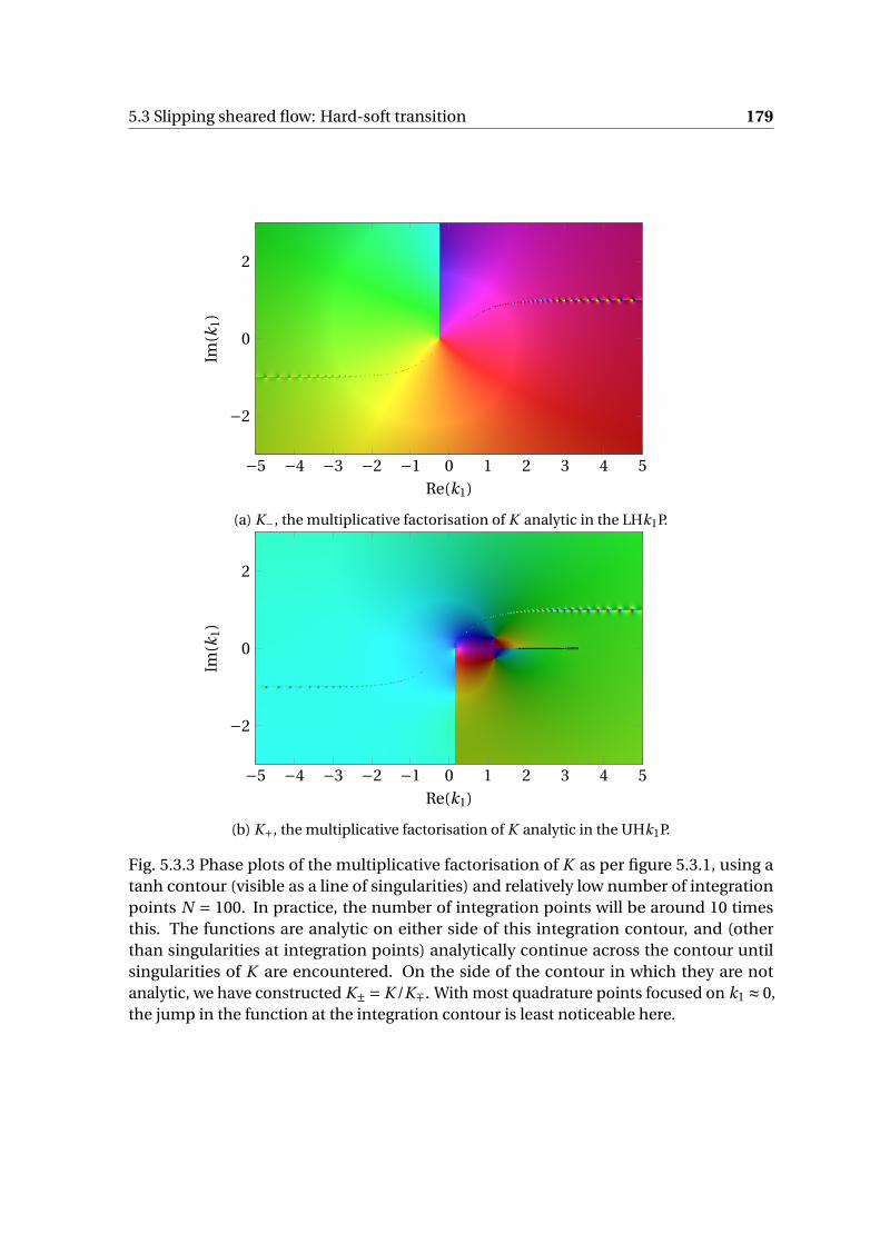
5.3 Slipping sheared flow: Hard-soft transition 179

−5 −4 −3 −2 −1 0 1 2 3 4 5

−2

0

2

Re(k1)

Im(k

1)

(a) K−, the multiplicative factorisation of K analytic in the LHk1P.

−5 −4 −3 −2 −1 0 1 2 3 4 5

−2

0

2

Re(k1)

Im(k

1)

(b) K+, the multiplicative factorisation of K analytic in the UHk1P.

Fig. 5.3.3 Phase plots of the multiplicative factorisation of K as per figure 5.3.1, using atanh contour (visible as a line of singularities) and relatively low number of integrationpoints N = 100. In practice, the number of integration points will be around 10 timesthis. The functions are analytic on either side of this integration contour, and (otherthan singularities at integration points) analytically continue across the contour untilsingularities of K are encountered. On the side of the contour in which they are notanalytic, we have constructed K± = K /K∓. With most quadrature points focused on k1 ≈ 0,the jump in the function at the integration contour is least noticeable here.

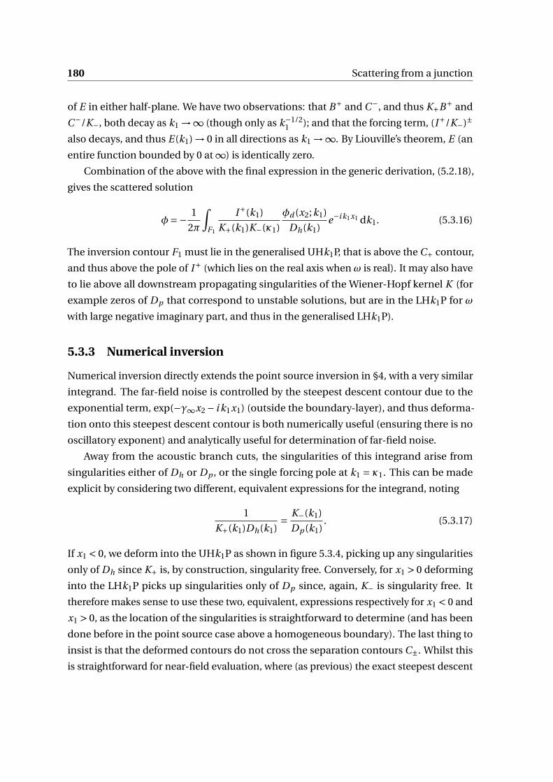
180 Scattering from a junction

of E in either half-plane. We have two observations: that B+ and C−, and thus K+B+ and

C−/K−, both decay as k1 →∞ (though only as k−1/21 ); and that the forcing term, (I+/K−)±

also decays, and thus E(k1) → 0 in all directions as k1 →∞. By Liouville’s theorem, E (an

entire function bounded by 0 at ∞) is identically zero.

Combination of the above with the final expression in the generic derivation, (5.2.18),

gives the scattered solution

φ=− 1

2π

∫F1

I+(k1)

K+(k1)K−(κ1)

φd (x2;k1)

Dh(k1)e−i k1x1 dk1. (5.3.16)

The inversion contour F1 must lie in the generalised UHk1P, that is above the C+ contour,

and thus above the pole of I+ (which lies on the real axis when ω is real). It may also have

to lie above all downstream propagating singularities of the Wiener-Hopf kernel K (for

example zeros of Dp that correspond to unstable solutions, but are in the LHk1P for ω

with large negative imaginary part, and thus in the generalised LHk1P).

5.3.3 Numerical inversion

Numerical inversion directly extends the point source inversion in §4, with a very similar

integrand. The far-field noise is controlled by the steepest descent contour due to the

exponential term, exp(−γ∞x2 − i k1x1) (outside the boundary-layer), and thus deforma-

tion onto this steepest descent contour is both numerically useful (ensuring there is no

oscillatory exponent) and analytically useful for determination of far-field noise.

Away from the acoustic branch cuts, the singularities of this integrand arise from

singularities either of Dh or Dp , or the single forcing pole at k1 = κ1. This can be made

explicit by considering two different, equivalent expressions for the integrand, noting

1

K+(k1)Dh(k1)= K−(k1)

Dp (k1). (5.3.17)

If x1 < 0, we deform into the UHk1P as shown in figure 5.3.4, picking up any singularities

only of Dh since K+ is, by construction, singularity free. Conversely, for x1 > 0 deforming

into the LHk1P picks up singularities only of Dp since, again, K− is singularity free. It

therefore makes sense to use these two, equivalent, expressions respectively for x1 < 0 and

x1 > 0, as the location of the singularities is straightforward to determine (and has been

done before in the point source case above a homogeneous boundary). The last thing to

insist is that the deformed contours do not cross the separation contours C±. Whilst this

is straightforward for near-field evaluation, where (as previous) the exact steepest descent

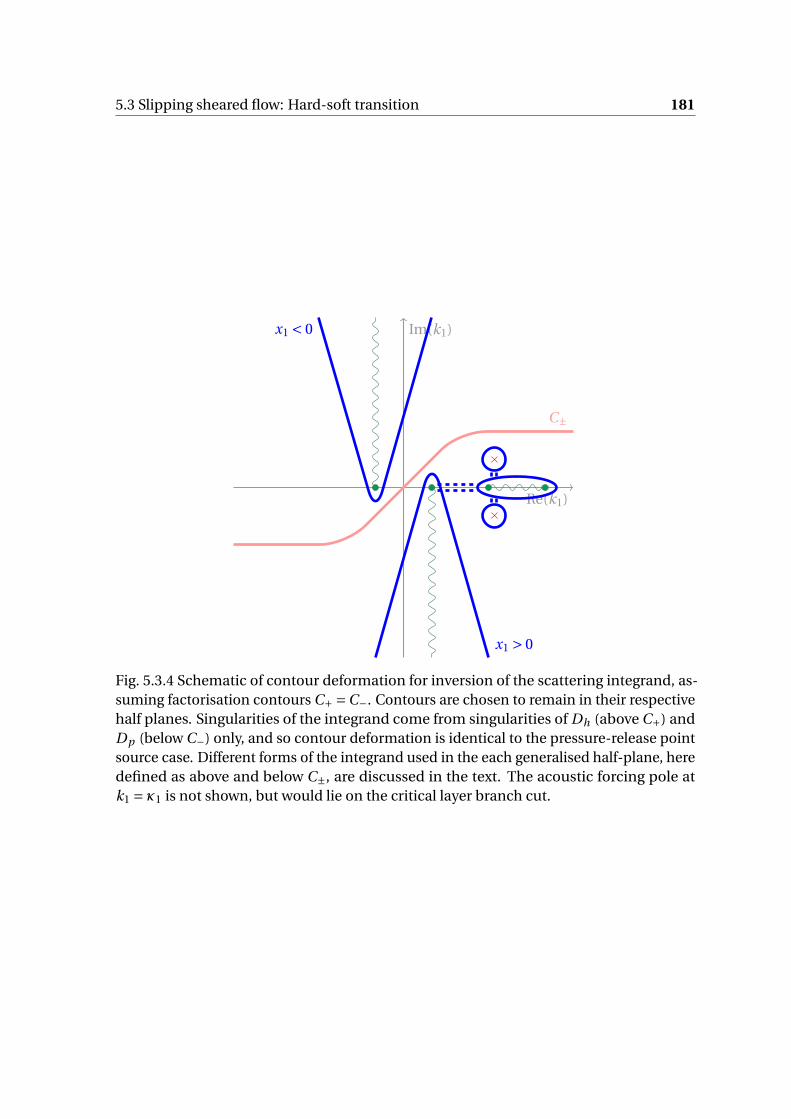
5.3 Slipping sheared flow: Hard-soft transition 181

Re(k1)

Im(k1)

C±

x1 < 0

x1 > 0

Fig. 5.3.4 Schematic of contour deformation for inversion of the scattering integrand, as-suming factorisation contours C+ =C−. Contours are chosen to remain in their respectivehalf planes. Singularities of the integrand come from singularities of Dh (above C+) andDp (below C−) only, and so contour deformation is identical to the pressure-release pointsource case. Different forms of the integrand used in the each generalised half-plane, heredefined as above and below C±, are discussed in the text. The acoustic forcing pole atk1 = κ1 is not shown, but would lie on the critical layer branch cut.

182 Scattering from a junction

contour is not used, when doing far-field evaluation this will require care with quantifying

where the saddle point is with respect to the separation contour, as discussed below.

We are now in a position to compute the near field solution by numerically computing

the inversion. The unstable case treated as a generic example is inverted and shown in

figures 5.3.5, with the excited pressure mode growing exponentially downstream seen in

the scattered component figure 5.3.5b. The full solution (figure 5.3.5a) clearly shows the

satisfaction of the pressure-release boundary condition for x1 > 0, and the purely acoustic

radiating component can be isolated by focus purely on the steepest descent contours (or,

in this case, the approximation looping each acoustic branch cut).

The same scattering problem (with the same slipping parabolic background flow)

is shown for higher frequency in figure 5.3.6, a stable configuration (as shown in the

pressure-release considerations in §4). In this case, the incident vortex sheet is changed

little over the junction and dominates the solution, and so only the scattered component

is shown. A clear radiating wavefront can be seen, due to the steepest descent contours,

and in turn the saddle point.

5.3.4 Far-field noise

Noting the clear radiation pattern from the junction point itself, the natural question

is to investigate the acoustic radiation generated by the junction itself. If this is large,

any noise-reduction advantage to use of a short section of lining may be removed by the

leading- and trailing-edges of the lining itself. This analysis can be performed using the

steepest descent method, and in turn focusing on the saddle point contribution, due to

the identical exponent in the integrand (outside the boundary-layer) as the point source

integrand (see, for example, (4.3.8)) and thus we proceed using the same saddle point

method, and steepest descent contours, as §4.3.1.

Given the work already done on steepest descent and far-field noise, previous work

transfers across with only the single caveat of being careful with generalised half planes.

This is sketched in figure 5.3.7, showing the saddle point passing from one half plane

to the other. To avoid numerical error near the separation contours, the two different,

equivalent, expressions in (5.3.17) are used respectively in the (generalised) Upper and

Lower Half k1-planes, with a check that the two routines agree for θ such that the saddle

point, k1s(θ), lies between the two separation contours.

The junction itself is the primary acoustic source. This leads to a single lobe in far-

field directivity plots, as there is no corresponding image source to consider (as per the

point source case) since the acoustic source lies on the wall itself. When considering,

for example, |p ′|, it is reasonable to expect this directivity to be directed upstream, as

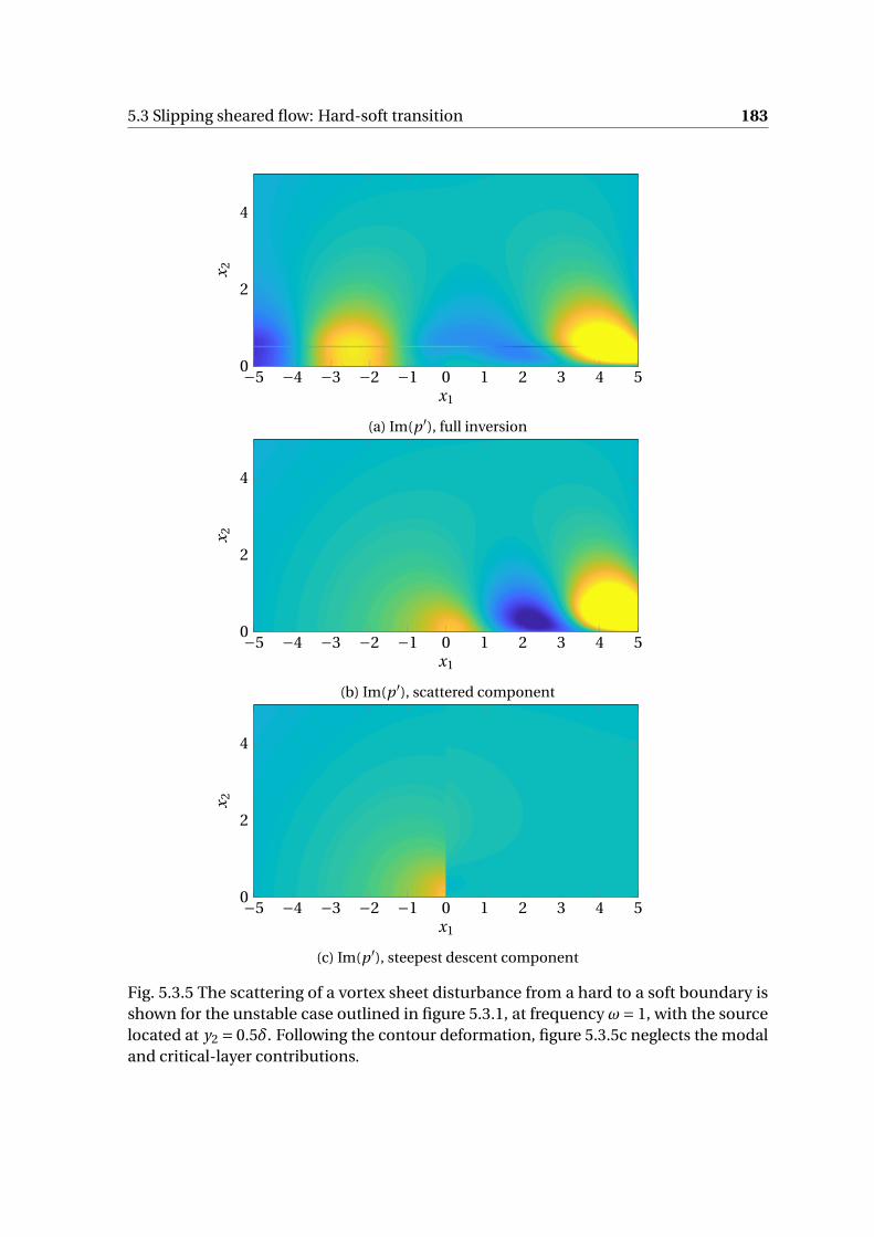
5.3 Slipping sheared flow: Hard-soft transition 183

−5 −4 −3 −2 −1 0 1 2 3 4 50

2

4

x1

x 2

(a) Im(p ′), full inversion

−5 −4 −3 −2 −1 0 1 2 3 4 50

2

4

x1

x 2

(b) Im(p ′), scattered component

−5 −4 −3 −2 −1 0 1 2 3 4 50

2

4

x1

x 2

(c) Im(p ′), steepest descent component

Fig. 5.3.5 The scattering of a vortex sheet disturbance from a hard to a soft boundary isshown for the unstable case outlined in figure 5.3.1, at frequency ω= 1, with the sourcelocated at y2 = 0.5δ. Following the contour deformation, figure 5.3.5c neglects the modaland critical-layer contributions.

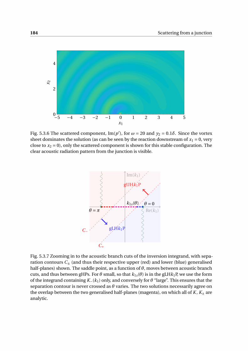
184 Scattering from a junction

−5 −4 −3 −2 −1 0 1 2 3 4 50

2

4

x1

x 2

Fig. 5.3.6 The scattered component, Im(p ′), for ω = 20 and y2 = 0.1δ. Since the vortexsheet dominates the solution (as can be seen by the reaction downstream of x1 = 0, veryclose to x2 = 0), only the scattered component is shown for this stable configuration. Theclear acoustic radiation pattern from the junction is visible.

Re(k1)

Im(k1)

C−

C+

gUHk1P

gLHk1P

k1s(θ) θ = 0

θ =π

Fig. 5.3.7 Zooming in to the acoustic branch cuts of the inversion integrand, with sepa-ration contours C± (and thus their respective upper (red) and lower (blue) generalisedhalf-planes) shown. The saddle point, as a function of θ, moves between acoustic branchcuts, and thus between gHPs. For θ small, so that k1s(θ) is in the gLHk1P, we use the formof the integrand containing K−(k1) only, and conversely for θ “large”. This ensures that theseparation contour is never crossed as θ varies. The two solutions necessarily agree onthe overlap between the two generalised half-planes (magenta), on which all of K , K± areanalytic.

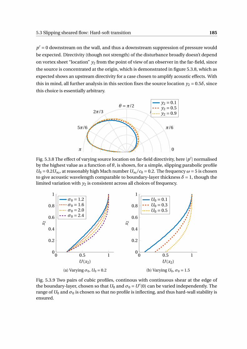
5.3 Slipping sheared flow: Hard-soft transition 185

p ′ = 0 downstream on the wall, and thus a downstream suppression of pressure would

be expected. Directivity (though not strength) of the disturbance broadly doesn’t depend

on vortex sheet “location” y2 from the point of view of an observer in the far-field, since

the source is concentrated at the origin, which is demonstrated in figure 5.3.8, which as

expected shows an upstream directivity for a case chosen to amplify acoustic effects. With

this in mind, all further analysis in this section fixes the source location y2 = 0.5δ, since

this choice is essentially arbitrary.

0

π/6

π/3θ =π/2

π

5π/6

2π/3

y2 = 0.1y2 = 0.5y2 = 0.9

Fig. 5.3.8 The effect of varying source location on far-field directivity, here |p ′| normalisedby the highest value as a function of θ, is shown, for a simple, slipping parabolic profileU0 = 0.2U∞, at reasonably high Mach number U∞/c0 = 0.2. The frequency ω= 5 is chosento give acoustic wavelength comparable to boundary-layer thickness δ= 1, though thelimited variation with y2 is consistent across all choices of frequency.

0 0.5 10

0.2

0.4

0.6

0.8

1

U (x2)

x 2

σ0 = 1.2σ0 = 1.6σ0 = 2.0σ0 = 2.4

(a) Varying σ0, U0 = 0.2

0 0.5 10

0.2

0.4

0.6

0.8

1

U (x2)

x 2

U0 = 0.1U0 = 0.3U0 = 0.5

(b) Varying U0, σ0 = 1.5

Fig. 5.3.9 Two pairs of cubic profiles, continous with continuous shear at the edge ofthe boundary-layer, chosen so that U0 and σ0 =U ′(0) can be varied independently. Therange of U0 and σ0 is chosen so that no profile is inflecting, and thus hard-wall stability isensured.

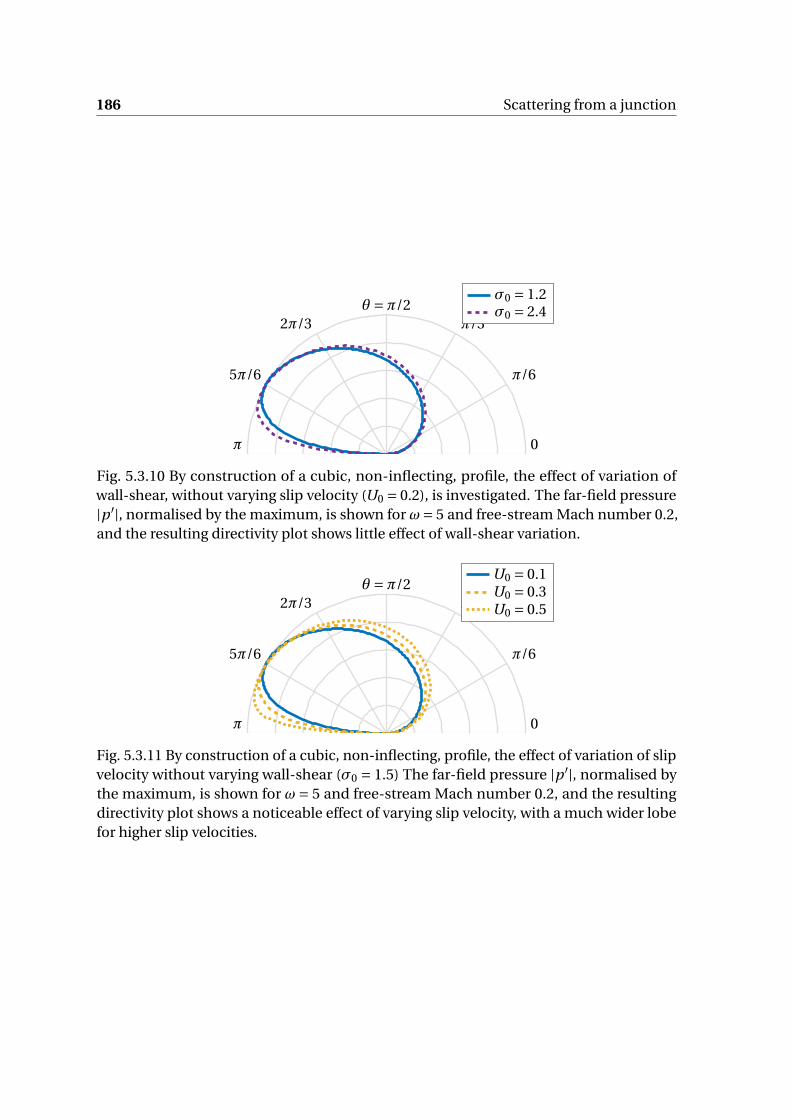
186 Scattering from a junction

0

π/6

π/3θ =π/2

π

5π/6

2π/3

σ0 = 1.2σ0 = 2.4

Fig. 5.3.10 By construction of a cubic, non-inflecting, profile, the effect of variation ofwall-shear, without varying slip velocity (U0 = 0.2), is investigated. The far-field pressure|p ′|, normalised by the maximum, is shown for ω= 5 and free-stream Mach number 0.2,and the resulting directivity plot shows little effect of wall-shear variation.

0

π/6

π/3θ =π/2

π

5π/6

2π/3

U0 = 0.1U0 = 0.3U0 = 0.5

Fig. 5.3.11 By construction of a cubic, non-inflecting, profile, the effect of variation of slipvelocity without varying wall-shear (σ0 = 1.5) The far-field pressure |p ′|, normalised bythe maximum, is shown for ω= 5 and free-stream Mach number 0.2, and the resultingdirectivity plot shows a noticeable effect of varying slip velocity, with a much wider lobefor higher slip velocities.

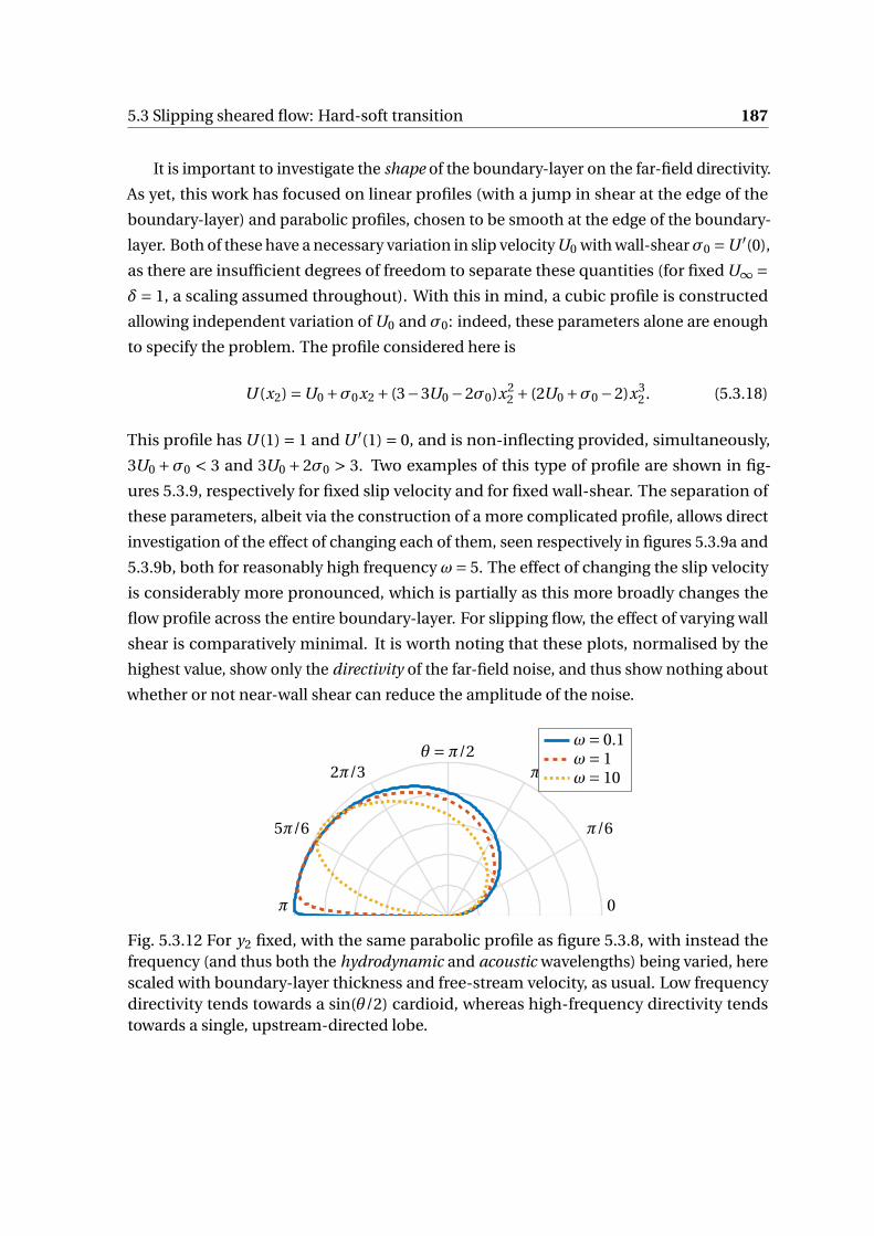
5.3 Slipping sheared flow: Hard-soft transition 187

It is important to investigate the shape of the boundary-layer on the far-field directivity.

As yet, this work has focused on linear profiles (with a jump in shear at the edge of the

boundary-layer) and parabolic profiles, chosen to be smooth at the edge of the boundary-

layer. Both of these have a necessary variation in slip velocity U0 with wall-shearσ0 =U ′(0),

as there are insufficient degrees of freedom to separate these quantities (for fixed U∞ =δ= 1, a scaling assumed throughout). With this in mind, a cubic profile is constructed

allowing independent variation of U0 and σ0: indeed, these parameters alone are enough

to specify the problem. The profile considered here is

U (x2) =U0 +σ0x2 + (3−3U0 −2σ0)x22 + (2U0 +σ0 −2)x3

2 . (5.3.18)

This profile has U (1) = 1 and U ′(1) = 0, and is non-inflecting provided, simultaneously,

3U0 +σ0 < 3 and 3U0 +2σ0 > 3. Two examples of this type of profile are shown in fig-

ures 5.3.9, respectively for fixed slip velocity and for fixed wall-shear. The separation of

these parameters, albeit via the construction of a more complicated profile, allows direct

investigation of the effect of changing each of them, seen respectively in figures 5.3.9a and

5.3.9b, both for reasonably high frequency ω= 5. The effect of changing the slip velocity

is considerably more pronounced, which is partially as this more broadly changes the

flow profile across the entire boundary-layer. For slipping flow, the effect of varying wall

shear is comparatively minimal. It is worth noting that these plots, normalised by the

highest value, show only the directivity of the far-field noise, and thus show nothing about

whether or not near-wall shear can reduce the amplitude of the noise.

0

π/6

π/3θ =π/2

π

5π/6

2π/3

ω= 0.1ω= 1ω= 10

Fig. 5.3.12 For y2 fixed, with the same parabolic profile as figure 5.3.8, with instead thefrequency (and thus both the hydrodynamic and acoustic wavelengths) being varied, herescaled with boundary-layer thickness and free-stream velocity, as usual. Low frequencydirectivity tends towards a sin(θ/2) cardioid, whereas high-frequency directivity tendstowards a single, upstream-directed lobe.

188 Scattering from a junction

0

π/6

π/3θ =π/2

π

5π/6

2π/3

ω= 2, λh ≈ 2.51ω= 4, λh ≈ 1.26ω= 6, λh ≈ 0.84ω= 8, λh ≈ 0.63ω= 10, λh ≈ 0.50

Fig. 5.3.13 The acoustic wavelength is fixed at 2π, so that c0 = ω for each plot. Thehydrodynamic lengthscale λh ≡ 2πU (y2)/ω is then allowed to vary.

0

π/6

π/3θ =π/2

π

5π/6

2π/3

Ma = 0.5Ma = 0.25Ma = 0.167Ma = 0.125Ma = 0.1

Fig. 5.3.14 As figure 5.3.13, except ω= 4 is fixed, fixing the hydrodynamic wavelength atapproximately 1.26 (and in turn, ensuring the red (solid) curves on both plots are thesame). The speeds of sound are as in the preceding plot, with acoustic wavelength herevarying from π to 5π.

5.3 Slipping sheared flow: Hard-soft transition 189

For a point source in sheared flow, the directivity was broadly controlled by the acous-

tic wavelength λa = 2π/k0 = 2πc0/ω, with some contributions from the hydrodynamic

wavelength λh = 2π/κ1 = 2πU (y2)/ω, which is smaller a factor of the Mach number. With

this, we focus on the effect of frequency variation on the far-field directivity, having identi-

fied the lack of impact from variation of source location and comparatively little effect

from variation of background profile. Varying frequency alone (whilst holding c0 and U

constant) produces figure 5.3.12, showing a broad trend from a cardioid sin(θ/2) profile

for low frequencies, to the single downstream-directed lobe for higher frequencies. As

before, there is only a single lobe: there is no real lengthscale imposed by the source to

cause an interference pattern as seen before (any “image” sources would be coincident

with the actual scattered source at the origin).

As before, it is useful to focus on varying each imposed lengthscale independently,

since varying ω varies both λh and λa . We firstly vary the hydrodynamic wavelength while

holding the acoustic lengthscale constant in figure 5.3.13. A short acoustic wavelength is

chosen to maximise any effect of the boundary-layer on the far-field acoustics, though this

in turn limits the possible range of values of λh (limited by required Ma < 1). Surprisingly,

even with the acoustic behaviour fixed, changing this alone has a large effect on the far-

field directivity. Shorter wavelength disturbances propagate more upstream. Whilst at

first glance this is linked to the boundary layer becoming more “incompressible” as c0

increases, this cannot entirely explain the effect as incompressibility is determined more

by the acoustic lengthscale which remains constant. This highlights the importance of the

source: even if its location might not be important, the induced lengthscale is.

Finally, focus on varying only the free-stream Mach number (and thus acoustic wave-

length) produces the very similar figure 5.3.14, chosen to overlap with the preceding case.

Whilst the qualitative trend is the same as holding the acoustic wavelength constant, the

effect is of a more directed high Mach number flow and of a more cardiod low Mach num-

ber flow, emphasising the importance of the acoustic wavelength on the scattering from

the junction: for a larger acoustic wavelength (smaller Mach number) the boundary-layer

effect is reduced, even for the same hydrodynamic wavelength, and a cardiod-type direc-

tivity profile is seen. This reduction to the “expected” incompressible/uniform solution

being more pronounced when the boundary-layer is acoustically compact (i.e. λa ≫ δ)

holds for even moderately large Mach number Ma, and is a far more pronounced effect

than the similar result for longer hydrodynamic wavelengths.

190 Scattering from a junction

5.4 Non-slipping sheared flow: Hard-soft transition

The previous section relied on the assumption that U0 = 0. This assumption is not critical

to the Wiener-Hopf analysis, indeed the resulting Wiener-Hopf equation (in the non-slip

case) is identical, with the kernel having the same definition, K = Dp /Dh . Issues arise

only from attempts to factorise this kernel, since the large k1 behaviour differs. This

fundamentally arises from the presence (or lack of) the term U0k1 in the transformed

convective derivative C , evaluated at the wall. For large k1 this term grows and dominates

(if U0 = 0) and so the non-appearance of this term in the non-slip kernel leads to greatly

differing large k1 asymptotics, and thus factorisation is more involved.

Otherwise, the mathematics for a non-slipping flow is identical, and the scattered

solution, due to a vortex sheet, is again given by (5.3.16), with suitably redefined K±.

5.4.1 Far-field kernel

Determination of the far-field behaviour can be determined by analogy with the piecewise-

linear, incompressible case. In this case, with exponential terms decaying rapidly, we

have

K ∼ i (k1σ0 −|k1|ω)

|k1|2(5.4.1)

which can immediately be seen by comparing the expressions for p ′ and v ′ in (3.3.7), for

example. Generalisation to the compressible case naïvely requires replacement of |k1| with

γ, which has identical far-field behaviour anyway (since U0 = 0 and so γ0 =√

k21 −ω2/c2

0 ,

at least for two-dimensional disturbances). With this, we have a far-field approximation,

for large k1, as

K ∼ i (k1σ0 −γ0ω)

γ20

(5.4.2)

with γ20 = k2

1 −k20 and wall shear σ0 =U ′(0). Unlike the previous case, there is no trivial

factorisation of this kernel as the difference k1σ0 −γ0ω has not be previously factorised.

We can, however, use the method outlined in §5.2.5, and find a numerical reduction of

the total kernel, which tends to unity at either end of the factorisation contour, using the

far-field behaviour from above.

We assume we have a separation contour (or contour) C(±)(s) tending towards ±∞s →±∞. Along this contour, we have

K ∼ i

|s|(σ0 ∓ω

). (5.4.3)

5.4 Non-slipping sheared flow: Hard-soft transition 191

This is the same far-field behavour as

K f = i (σ−ω)(k1 −kb+)−1/2+α+ (k1 −kb−)−1/2−α

− (5.4.4)

with exponent α defined as

α= 1

2πilog

(σ0 +ωσ0 −ω

). (5.4.5)

This is a complex number for ω complex. It is defined only up to the addition of a real

integer, which can be fixed to ensure that the winding number of K = K /K f is 0 along the

integration contour. The two branch points kb± are essentially arbitrary, provided they lie

respectively in the gL/UHk1P. In practice, we identify them with the branch points of γ0

as kb± =±√ω2/c2

0 −k23 , which avoids complication from multiple branch points of K in

different locations. The resulting reduced kernel, K = K /K f , therefore tends to 1 at either

end of the separation contour, and we can thus compute the multiplicative factorisation

of K by computing the additive factorisation of log(K ), as before. The factorisation of K

itself then follows from the trivial factoriation of K f , with

K f + = i (σ−ω)(k1 −kb+)−1/2+α+ , (5.4.6a)

K f − = (k1 −kb−)−1/2−α− . (5.4.6b)

The assignment of the leading constant i (σ−ω) is arbitrary, but for definiteness is included

in (5.4.6a). This factorisation is shown for a simple, non-slipping parabolic profile in

figure 5.4.1. Importantly, the continuity of log is demonstrated in figure 5.4.1b with the

principal value of α taken, demonstrating in this case no amendment due to winding

number is required.

5.4.2 Numerical inversion

As noted in the caption to figure 5.4.1, the critical layer for any no-slip profile extends

along k1 ∈ [ω/U∞,∞), if we integrate the governing differential equation along real x2.

By integrating along complex z (generalising x2 to the complex plane) we can deform

this critical-layer branch cut to a location of choice, with the leading branch cut fixed at

ω/U∞ but the path to ∞ changed. This allows not only a more accurate evaluation of

K±, by deforming the critical-layer (and the main source of numerical error) away from

the separation contour C±, but it allows more precise evaluation of the inversion integral

along the branch cut itself. Extending figure 5.3.4, the inversion contours for the no-slip

case are indicated, with colours here used to denote if the critical-layer is deformed into

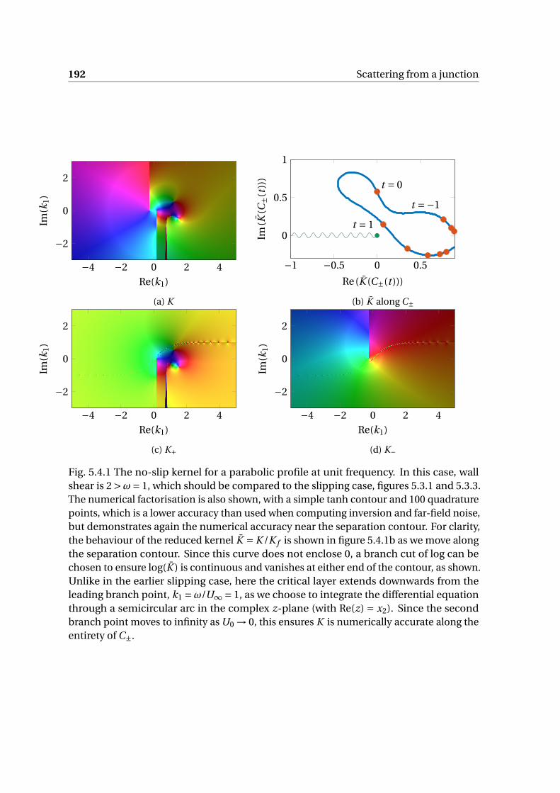
192 Scattering from a junction

−4 −2 0 2 4

−2

0

2

Re(k1)

Im(k

1)

(a) K

−1 −0.5 0 0.5

0

0.5

1

t =−1

t = 0

t = 1

Re(K (C±(t )))

Im(K

(C±(

t)))

(b) K along C±

−4 −2 0 2 4

−2

0

2

Re(k1)

Im(k

1)

(c) K+

−4 −2 0 2 4

−2

0

2

Re(k1)

Im(k

1)

(d) K−

Fig. 5.4.1 The no-slip kernel for a parabolic profile at unit frequency. In this case, wallshear is 2 >ω= 1, which should be compared to the slipping case, figures 5.3.1 and 5.3.3.The numerical factorisation is also shown, with a simple tanh contour and 100 quadraturepoints, which is a lower accuracy than used when computing inversion and far-field noise,but demonstrates again the numerical accuracy near the separation contour. For clarity,the behaviour of the reduced kernel K = K /K f is shown in figure 5.4.1b as we move alongthe separation contour. Since this curve does not enclose 0, a branch cut of log can bechosen to ensure log(K ) is continuous and vanishes at either end of the contour, as shown.Unlike in the earlier slipping case, here the critical layer extends downwards from theleading branch point, k1 =ω/U∞ = 1, as we choose to integrate the differential equationthrough a semicircular arc in the complex z-plane (with Re(z) = x2). Since the secondbranch point moves to infinity as U0 → 0, this ensures K is numerically accurate along theentirety of C±.

5.4 Non-slipping sheared flow: Hard-soft transition 193

the U/LHk1P (by deforming the z contour into the L/UHzP respectively). With the critical

layer contribution, the jump in the integrand over the critical-layer branch cut, tending

towards zero as |k1| gets large, this allows truncation of the critical-layer integral at some

finite, large, real k1.

Re(k1)

Im(k1)

C±

x1 < 0

x1 > 0

Fig. 5.4.2 Schematic of contour deformation in the no-slip case. Here, red contours (includ-ing the separation contour) indicate the integrand should be computed by integration inthe UHzP, so that the critical-layer is deformed into the LHk1P, and blue contours indicatethe converse. This allows precise evaluation of the integrand along both contours, andthus reduces numerical error in computation of the critical-layer contribution.

The final step required in the inversion process is to ensure the entire function, E(k1),

is suitably understood. This is made slightly more difficult by the complex exponent in

the far-field representation of the kernel K f ± (as per (5.4.6)), which can be used as a proxy

for the far-field behaviour of K± where relevant, as computed K± are analytic and tend to

unity at infinity in all directions.

We recall the definition of α in (5.4.5). If σ0 >ω> 0, then we have the logarithm of a

real number, and so α is imaginary (and with negative imaginary part, as σ0 −ω>σ0 +ω).

If, instead, ω>σ0 > 0, then α has a non-zero real part. The principal value gives this as

1/2, though if checking the curve K (C (t)) showed a non-zero winding number around

zero, this can be modified by an integer, though as per figure 5.4.1b, with ω= 1 <σ0 = 2,

the principal value suffices for this case. With this imaginary part negative in both cases,

194 Scattering from a junction

we split α= Re(α)− i b and then

K f ± ∼ (k1)−1/2∓i b+ (5.4.7)

for ω>σ, and

K f + ∼ (k1)−i b+ , (5.4.8)

K f − ∼ (k1)−1+i b− (5.4.9)

for ω<σ0. We now claim

(z)i x (5.4.10)

is bounded, regardless of choice of branch cut, for any real x. For z = r e iθ, we have

|zi x | = |r i x |e−xθ. (5.4.11)

The second part, e−xθ, is bounded either by its value at the minimum value of θ (for x < 0)

or at its maximum (for x > 0) as θ is sampled from some closed and bounded interval (for

a straight branch cut from 0 to ∞ in any direction). Then |r i x | = |e i x logr | = 1, as r is real

and positive. Thus, K f ± is, in the worst case, bounded by a constant, though 1/K− might

grow like k1. Provided B+, the pressure on the upstream surface, does not grow faster

than k1/21 (essentially arguing it is bounded, or at least is not particularly singular) then

the UHk1P definition of the entire function

E(k1) = K+B++(

I+

K−

)+(5.4.12)

must decay in the UHk1P, with the additive factorisation of the incident source inheriting

the behaviour of I+ only, and decaying as k−11 . Since any polynomial E will grow in the

UHk1P, E must be identically zero and we obtain exactly the same integrand as before, up

to replacement of K±.

Inverting along the slightly altered contours produces figure 5.4.3, for a parabolic

profile unstable above the pressure-release boundary downstream of x1 = 0. Two cases

are shown, with ω= 1 and ω= 4, respectively smaller and larger than wall shear σ0 = 2, to

demonstrate the validity of the solution in both cases.

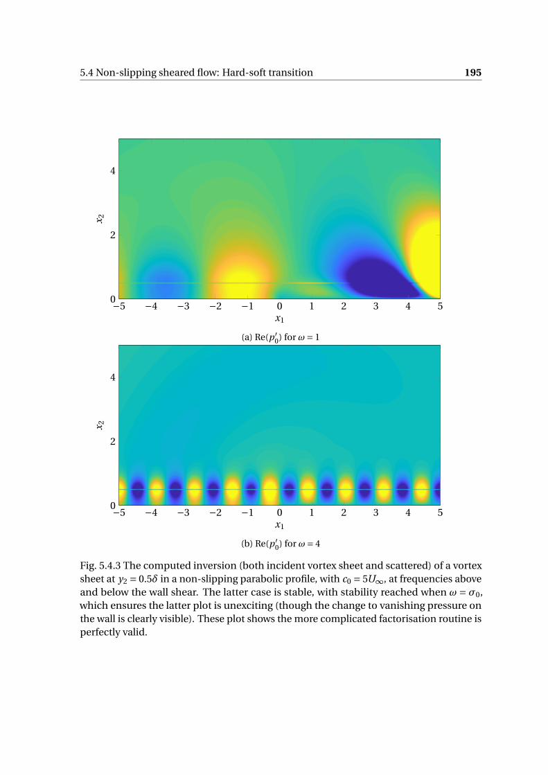
5.4 Non-slipping sheared flow: Hard-soft transition 195

−5 −4 −3 −2 −1 0 1 2 3 4 50

2

4

x1

x 2

(a) Re(p ′0) for ω= 1

−5 −4 −3 −2 −1 0 1 2 3 4 50

2

4

x1

x 2

(b) Re(p ′0) for ω= 4

Fig. 5.4.3 The computed inversion (both incident vortex sheet and scattered) of a vortexsheet at y2 = 0.5δ in a non-slipping parabolic profile, with c0 = 5U∞, at frequencies aboveand below the wall shear. The latter case is stable, with stability reached when ω = σ0,which ensures the latter plot is unexciting (though the change to vanishing pressure onthe wall is clearly visible). These plot shows the more complicated factorisation routine isperfectly valid.

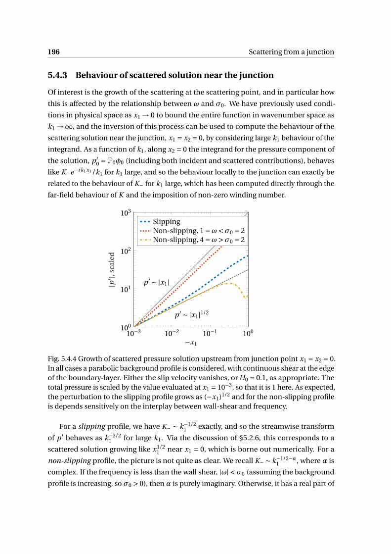
196 Scattering from a junction

5.4.3 Behaviour of scattered solution near the junction

Of interest is the growth of the scattering at the scattering point, and in particular how

this is affected by the relationship between ω and σ0. We have previously used condi-

tions in physical space as x1 → 0 to bound the entire function in wavenumber space as

k1 →∞, and the inversion of this process can be used to compute the behaviour of the

scattering solution near the junction, x1 = x2 = 0, by considering large k1 behaviour of the

integrand. As a function of k1, along x2 = 0 the integrand for the pressure component of

the solution, p ′0 =P0φ0 (including both incident and scattered contributions), behaves

like K−e−i k1x1 /k1 for k1 large, and so the behaviour locally to the junction can exactly be

related to the behaviour of K− for k1 large, which has been computed directly through the

far-field behaviour of K and the imposition of non-zero winding number.

10−3 10−2 10−1 100100

101

102

103

p ′ ∼ |x1|

p ′ ∼ |x1|1/2

−x1

|p′ |,

scal

ed

SlippingNon-slipping, 1 =ω<σ0 = 2Non-slipping, 4 =ω>σ0 = 2

Fig. 5.4.4 Growth of scattered pressure solution upstream from junction point x1 = x2 = 0.In all cases a parabolic background profile is considered, with continuous shear at the edgeof the boundary-layer. Either the slip velocity vanishes, or U0 = 0.1, as appropriate. Thetotal pressure is scaled by the value evaluated at x1 = 10−3, so that it is 1 here. As expected,the perturbation to the slipping profile grows as (−x1)1/2 and for the non-slipping profileis depends sensitively on the interplay between wall-shear and frequency.

For a slipping profile, we have K− ∼ k−1/21 exactly, and so the streamwise transform

of p ′ behaves as k−3/21 for large k1. Via the discussion of §5.2.6, this corresponds to a

scattered solution growing like x1/21 near x1 = 0, which is borne out numerically. For a

non-slipping profile, the picture is not quite as clear. We recall K− ∼ k−1/2−α1 , where α is

complex. If the frequency is less than the wall shear, |ω| <σ0 (assuming the background

profile is increasing, so σ0 > 0), then α is purely imaginary. Otherwise, it has a real part of

5.4 Non-slipping sheared flow: Hard-soft transition 197

1/2 (to ensure that the winding number criterion is satisfied). In either case, p ′ ∼ x1/2+α1 .

When the frequency is large, larger than the wall shear, the scattered pressure grows

(upstream, since it vanishes downstream) like x1, with some modifications from the

remaining imaginary power. These three cases, slipping and non-slipping with ω≷σ0 are

considered numerically in figure 5.4.4, producing the results expected. In particular, for

low frequency growth is much more like |x1|, though the complex contribution ensures it

is slightly less than this. This is consistent with previous work suggesting a growth rate

between |x1|1/2 and |x1|.

5.4.4 Far-field noise

Computation of far-field noise proceeds exactly as in the previous section §5.3, with

suitably modified K , and as such there is no need to go into details here. Since evaluation

of the far-field noise requires, for each observer angle, evaluation at single wavenumber

ks(θ), it is much more rapid than computing the full near-field inversion. With this in

mind, we can use the far-field noise to focus on two specific problems of this setup: firstly

whether the no-slip limit is in fact the limit of the preceding section as U0 → 0, which

physically we would expect; and secondly what happens in the long-wavelength limit

(comparing to previous work such as [101], which suggested non-trivial far-field behaviour

when directly factorising the incompressible kernel K , rather than considering the limit of

large finite c0).

5.4.5 The consistency of the no-slip limit

The mathematical routine is fundamentally different depending on whether U0 = 0 or U0 =0, though physically we wouldn’t expect any abrupt change in the solution. Computation

of far-field noise readily allows testing of this limit. This is readily investigated as per

figure 5.4.5, which uses both the slipping and non-slipping mathematical routines. In the

limit U0 → 0, the solution changes continuously, as physical intuition might suggest. This

holds broadly across all frequencies, the choice of frequency is to emphasise the similarity

in the limit.

5.4.6 The incompressible (long-wavelength) limit

This chapter has, as yet, been focused on the compressible case and the associated acoustic

potential φ, in contrast to the opening work of §3, which looked at long-wavelength

disturbances which could be regarded as, on the boundary-layer scale, incompressible.

198 Scattering from a junction

0

π/6

π/3θ =π/2

π

5π/6

2π/3

U0 = 0.001U0 = 0.0001U0 = 0

Fig. 5.4.5 Considering a parabolic profile with frequency ω = 5 and free-stream Machnumber 0.2. The slip velocity U0 is relaxed to zero and the directivity of the resultingscattered sound is plotted. The curves are essentially indistinguishable. There is thusno physical change in the far-field behaviour of the no-slip case. This result still holds ifω<σ0.

0

π/6

π/3θ =π/2

π

5π/6

2π/3

|p ′|/max(|p ′|), computedsin(θ/2)

Fig. 5.4.6 The far-field directivity for large speed of sound c0, here chosen to be 500U∞.Scattering from linear, non-slipping, background profile with unit shear, and frequencyω= 10 (though the result is consistent across all frequencies). For reference, the cardioiddirectivity sin(θ/2) is plotted, which shows precise agreement across for all θ <π.

5.4 Non-slipping sheared flow: Hard-soft transition 199

For a piecewise linear profile this substantially reduced the numerical complexity in

solving the governing ODE. Difficulties arise in the scattering problem, however, due to

the relaxation of γ=√

k21 −k2

0 to |k1|. The latter function has no contour stretching from

−∞ to ∞ on which it is analytic, since any contour must either pass over a branch cut or

through the branch point at 0. This causes problems with the Wiener-Hopf factorisation,

which implicitly assumes a strip of analyticity of the Wiener-Hopf kernel K , and therefore

some regularisation of |k1| is required to create a well-posed Wiener-Hopf problem.

This limit can be taken, however, in the numerical work we have already done, by

way of taking c0 to infinity. Strictly, we require the dual condition (as per the derivation

in §3) that k−10 = c0/ω ≫ δ (long acoustic wavelength, so that the boundary-layer is

acoustically compact) and that Ma2∞ =U 2∞/c2∞ ≪ 1, which permits non-negligible free-

stream velocities. For large but finite c0, there is nothing that prevents the derived routines

from being used, and an example of the far-field directivity is shown in figure 5.4.6. For

reference, the cardioid profile p ′ ∼ sin(θ/2) is also shown, which is exactly the profile that

would be expected for the scattering from a trailing-edge in no flow (with no boundary-

layer shear). As we shall see in the next chapter, the (symmetric) trailing-edge case is

analogous to the hard-soft junction, and so this result is unsurprising.

The incompressible framework is consistent in this limit. This resolves earlier difficul-

ties in factorising the apparent incompressible kernel directly [93, 101], which runs into

two problems. Firstly, the separation contours C± are pinched between the branches of

|k1| at the origin, which removes a well-defined Wiener-Hopf strip, and thus the factori-

sation can only be ever thought of in a limit, either of k3 → 0 (so√

k21 +k2

3 →|k1|) or the

limit of c0 →∞ (so γ=√

k21 −ω2/c2

0 →|k1|). It is possible to find factorisations that seem

to converge everywhere in this limit (in fact, the far-field factorisation used to reduce the

kernel for numerical evaluation), but the difficulty arises in evaluation of this resulting

kernel at k1 = 0. This is critical for far-field evaluation, as we saw in the earlier chapter §3.

Further, far-field evaluation in the compressible case with c0 finite requires evaluation

at the saddle point ks , which lies along a line connecting the two acoustic branch points.

This cannot possibly be done when c0 is infinite, as all these points collapse to k1 = 0. It is

therefore difficult to extract far-field information from a purely incompressible framework,

especially when evaluation of K at k1 = 0 is ill-defined.

With these two problems identified, the solution is to evaluate K alone as if it were

compressible, with c0 large (noting the convergence in the limit c0 →∞). All other func-

tions can be evaluated as if incompressible, which allows some analytic representation

of the solution, and preserves the useful modal structure seen in §3. However, given

factorisation of K is the most numerically difficult part of the computation, this approach

200 Scattering from a junction

seems unnecessarily roundabout and, unless the exact benefits of the modal structure

from a piecewise linear profile are required, there are insufficient gains from this approach

for it to be worthwhile.

5.5 Transition between two different lined surfaces

The hard-soft transition has been covered in detail primarily because of the straightfor-

ward application of the derived formulas, with the relevant dispersion functions Dh and

Dp covered in detail in previous chapters. The generic setup in the opening section,

§5.2, allows for more complicated linear boundary conditions with little further work, the

majority of the work focusing on identification of the far-field behaviour of the relevant

Wiener-Hopf kernel (and relating concerns of winding numbers and behaviour of the

entire function E ). With this in mind, this section focused on the generic case of scattering

from a transition between two lined surfaces, with arbitrary impedances Zu and Zd , up-

stream and downstream respectively. It opens with a brief discussion of the special case of

a soft-hard transition, the inverse of the case seen above, which is the special case Zu = 0

and Zd =∞.

5.5.1 Soft to hard transition

We previously considered generalised Upper and Lower Half Planes. For the generic kernel

K = Dd /Du , we required that zeros of Dd and of Du , respectively zeros and poles of K , lie

in the half-plane as determined by a Briggs-Bers analysis (i.e. the half-plane they lie in for

large negative Im(ω)). The alternate problem of scattering from the formerly downstream

boundary condition to the formerly upstream boundary condition involves the inverse

kernel K −1, which has zeros and poles at the zeros of Du and Dd respectively, but which

lie in exactly the same generalised half planes as before. The factorisation of K −1 then

follows exactly the same procedure as factorising K , with resulting factors simply K −1± ,

which are trivially synthesised from the already computed splitfunctions. Essentially, the

careful causality considerations in the preceding section ensure that the problem with

flipped boundary conditions is a trivial extension of the previous problem.

5.5.2 Impedance to impedance transition

We now consider the generic case of an upstream boundary with impedance Zu (for

x1 < 0) and a downstream boundary with impedance Zd . Provided these are not 0 (a

pressure-release boundary) or ∞ (a hard-wall boundary) the analysis that follows is in

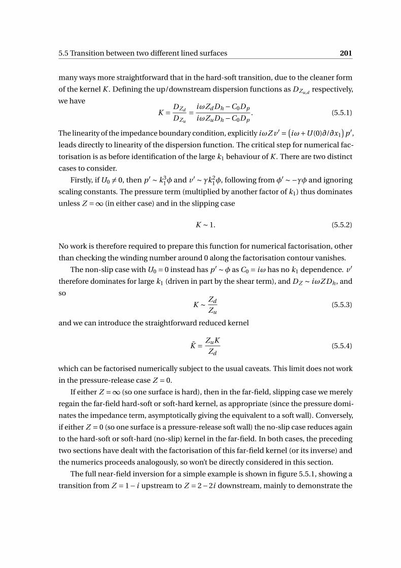
5.5 Transition between two different lined surfaces 201

many ways more straightforward that in the hard-soft transition, due to the cleaner form

of the kernel K . Defining the up/downstream dispersion functions as DZu,d respectively,

we have

K = DZd

DZu

= iωZd Dh −C0Dp

iωZuDh −C0Dp. (5.5.1)

The linearity of the impedance boundary condition, explicitly iωZ v ′ = (iω+U (0)∂/∂x1

)p ′,

leads directly to linearity of the dispersion function. The critical step for numerical fac-

torisation is as before identification of the large k1 behaviour of K . There are two distinct

cases to consider.

Firstly, if U0 = 0, then p ′ ∼ k31φ and v ′ ∼ γk2

1φ, following from φ′ ∼−γφ and ignoring

scaling constants. The pressure term (multiplied by another factor of k1) thus dominates

unless Z =∞ (in either case) and in the slipping case

K ∼ 1. (5.5.2)

No work is therefore required to prepare this function for numerical factorisation, other

than checking the winding number around 0 along the factorisation contour vanishes.

The non-slip case with U0 = 0 instead has p ′ ∼φ as C0 = iω has no k1 dependence. v ′

therefore dominates for large k1 (driven in part by the shear term), and DZ ∼ iωZ Dh , and

so

K ∼ Zd

Zu(5.5.3)

and we can introduce the straightforward reduced kernel

K = ZuK

Zd(5.5.4)

which can be factorised numerically subject to the usual caveats. This limit does not work

in the pressure-release case Z = 0.

If either Z =∞ (so one surface is hard), then in the far-field, slipping case we merely

regain the far-field hard-soft or soft-hard kernel, as appropriate (since the pressure domi-

nates the impedance term, asymptotically giving the equivalent to a soft wall). Conversely,

if either Z = 0 (so one surface is a pressure-release soft wall) the no-slip case reduces again

to the hard-soft or soft-hard (no-slip) kernel in the far-field. In both cases, the preceding

two sections have dealt with the factorisation of this far-field kernel (or its inverse) and

the numerics proceeds analogously, so won’t be directly considered in this section.

The full near-field inversion for a simple example is shown in figure 5.5.1, showing a

transition from Z = 1− i upstream to Z = 2−2i downstream, mainly to demonstrate the

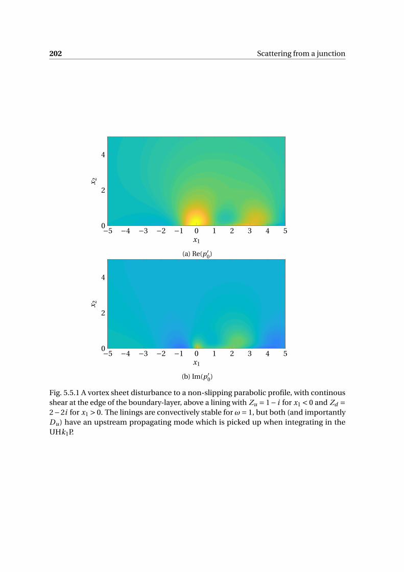
202 Scattering from a junction

−5 −4 −3 −2 −1 0 1 2 3 4 50

2

4

x1

x 2

(a) Re(p ′0)

−5 −4 −3 −2 −1 0 1 2 3 4 50

2

4

x1

x 2

(b) Im(p ′0)

Fig. 5.5.1 A vortex sheet disturbance to a non-slipping parabolic profile, with continousshear at the edge of the boundary-layer, above a lining with Zu = 1− i for x1 < 0 and Zd =2−2i for x1 > 0. The linings are convectively stable for ω= 1, but both (and importantlyDu) have an upstream propagating mode which is picked up when integrating in theUHk1P.

5.6 Restabilisation of unstable modes 203

validity of the code, and in particular the answer is consistent for x1 ≷ 0 (when the choice

of contours changes). Only the scattered component, focused on the origin, is displayed,

since the scattered solution is much smaller in magnitude than the incident solution

(and so is essentially not visible on the full plot). This case differs slightly from previous

work, since, with the frequency and profile chosen, the lined walls have two surface mode

solutions, one with Re(k1) < 0. This can be shown to be upstream propagating, and thus

the zero of Du should be picked up when integrating in the UHk1P. Two modal solutions

therefore originate at x1 = 0, one propagating to the right (a zero of Dd ) and one to the left

(a zero of Du), both exponentially decaying downstream.

0

π/6

π/3θ =π/2

π

5π/6

2π/3

R = 0.1R = 0.5R = 2R = 10Hard-soft

Fig. 5.5.2 The scattering from an impedance-impedance junction, with Zu = (1− i )/R andZd = R(1− i ). A non-slipping parabolic background profile, with free-speed Ma = 0.2, isconsidered as before, at frequency ω= 1.

Finally, far-field scattered noise can be computed in the usual way. We can use this

to demonstrate the consistency of Z → 0 (pressure-release) and Z →∞ (hard-wall). This

is done in figure 5.5.2, with Zu increasing as Zd decreasing, showing the single lobe

directivity moving from upstream to downstream. It is worth noting the plot is not quite

symmetric in R → R−1, with a general downstream lean to the lobes. For reference the

hard-soft junction is plotted, which is the limit of vanishing R, and can indeed be shown

to be obtained in the limit of small, non-zero R. We are satisfied that the impedance

case accurately recaptures the previous hard-soft transition, despite the fundamentally

different factorisation routines.

5.6 Restabilisation of unstable modes

It was briefly noted in the previous section, §5.5.1, that the soft-to-hard transition is

mathematically a straightforward extension of the hard-to-soft transition, with the all-

important Wiener-Hopf kernel simply the reciprocal of the earlier kernel. We can take

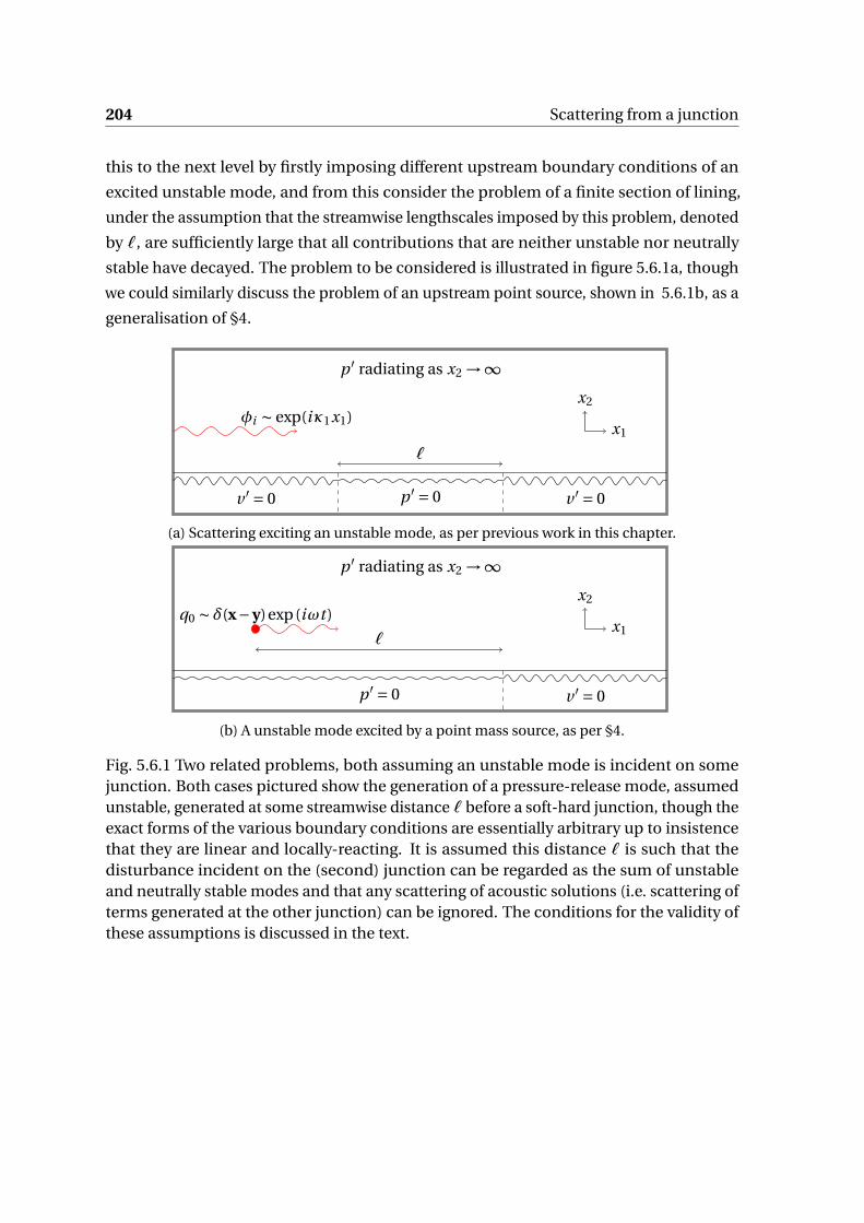
204 Scattering from a junction

this to the next level by firstly imposing different upstream boundary conditions of an

excited unstable mode, and from this consider the problem of a finite section of lining,

under the assumption that the streamwise lengthscales imposed by this problem, denoted

by ℓ, are sufficiently large that all contributions that are neither unstable nor neutrally

stable have decayed. The problem to be considered is illustrated in figure 5.6.1a, though

we could similarly discuss the problem of an upstream point source, shown in 5.6.1b, as a

generalisation of §4.

x2

x1φi ∼ exp(iκ1x1)

ℓ

v ′ = 0 v ′ = 0p ′ = 0

p ′ radiating as x2 →∞

(a) Scattering exciting an unstable mode, as per previous work in this chapter.

x2

x1q0 ∼ δ(x−y)exp(iωt )

ℓ

v ′ = 0p ′ = 0

p ′ radiating as x2 →∞

(b) A unstable mode excited by a point mass source, as per §4.

Fig. 5.6.1 Two related problems, both assuming an unstable mode is incident on somejunction. Both cases pictured show the generation of a pressure-release mode, assumedunstable, generated at some streamwise distance ℓ before a soft-hard junction, though theexact forms of the various boundary conditions are essentially arbitrary up to insistencethat they are linear and locally-reacting. It is assumed this distance ℓ is such that thedisturbance incident on the (second) junction can be regarded as the sum of unstableand neutrally stable modes and that any scattering of acoustic solutions (i.e. scattering ofterms generated at the other junction) can be ignored. The conditions for the validity ofthese assumptions is discussed in the text.

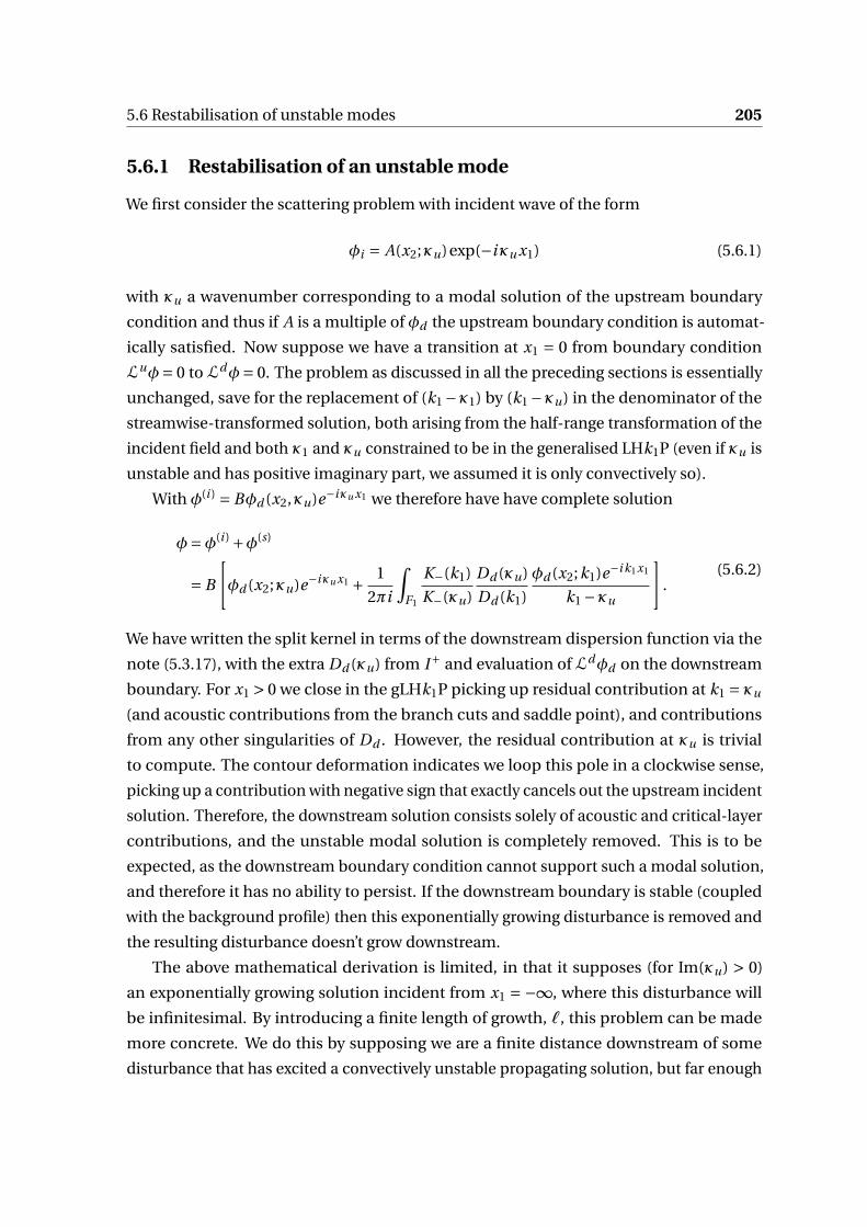
5.6 Restabilisation of unstable modes 205

5.6.1 Restabilisation of an unstable mode

We first consider the scattering problem with incident wave of the form

φi = A(x2;κu)exp(−iκu x1) (5.6.1)

with κu a wavenumber corresponding to a modal solution of the upstream boundary

condition and thus if A is a multiple of φd the upstream boundary condition is automat-

ically satisfied. Now suppose we have a transition at x1 = 0 from boundary condition

Luφ= 0 to Ldφ= 0. The problem as discussed in all the preceding sections is essentially

unchanged, save for the replacement of (k1 −κ1) by (k1 −κu) in the denominator of the

streamwise-transformed solution, both arising from the half-range transformation of the

incident field and both κ1 and κu constrained to be in the generalised LHk1P (even if κu is

unstable and has positive imaginary part, we assumed it is only convectively so).

With φ(i ) = Bφd (x2,κu)e−iκu x1 we therefore have have complete solution

φ=φ(i ) +φ(s)

= B

[φd (x2;κu)e−iκu x1 + 1

2πi

∫F1

K−(k1)

K−(κu)

Dd (κu)

Dd (k1)

φd (x2;k1)e−i k1x1

k1 −κu

].

(5.6.2)

We have written the split kernel in terms of the downstream dispersion function via the

note (5.3.17), with the extra Dd (κu) from I+ and evaluation of Ldφd on the downstream

boundary. For x1 > 0 we close in the gLHk1P picking up residual contribution at k1 = κu

(and acoustic contributions from the branch cuts and saddle point), and contributions

from any other singularities of Dd . However, the residual contribution at κu is trivial

to compute. The contour deformation indicates we loop this pole in a clockwise sense,

picking up a contribution with negative sign that exactly cancels out the upstream incident

solution. Therefore, the downstream solution consists solely of acoustic and critical-layer

contributions, and the unstable modal solution is completely removed. This is to be

expected, as the downstream boundary condition cannot support such a modal solution,

and therefore it has no ability to persist. If the downstream boundary is stable (coupled

with the background profile) then this exponentially growing disturbance is removed and

the resulting disturbance doesn’t grow downstream.

The above mathematical derivation is limited, in that it supposes (for Im(κu) > 0)

an exponentially growing solution incident from x1 = −∞, where this disturbance will

be infinitesimal. By introducing a finite length of growth, ℓ, this problem can be made

more concrete. We do this by supposing we are a finite distance downstream of some

disturbance that has excited a convectively unstable propagating solution, but far enough

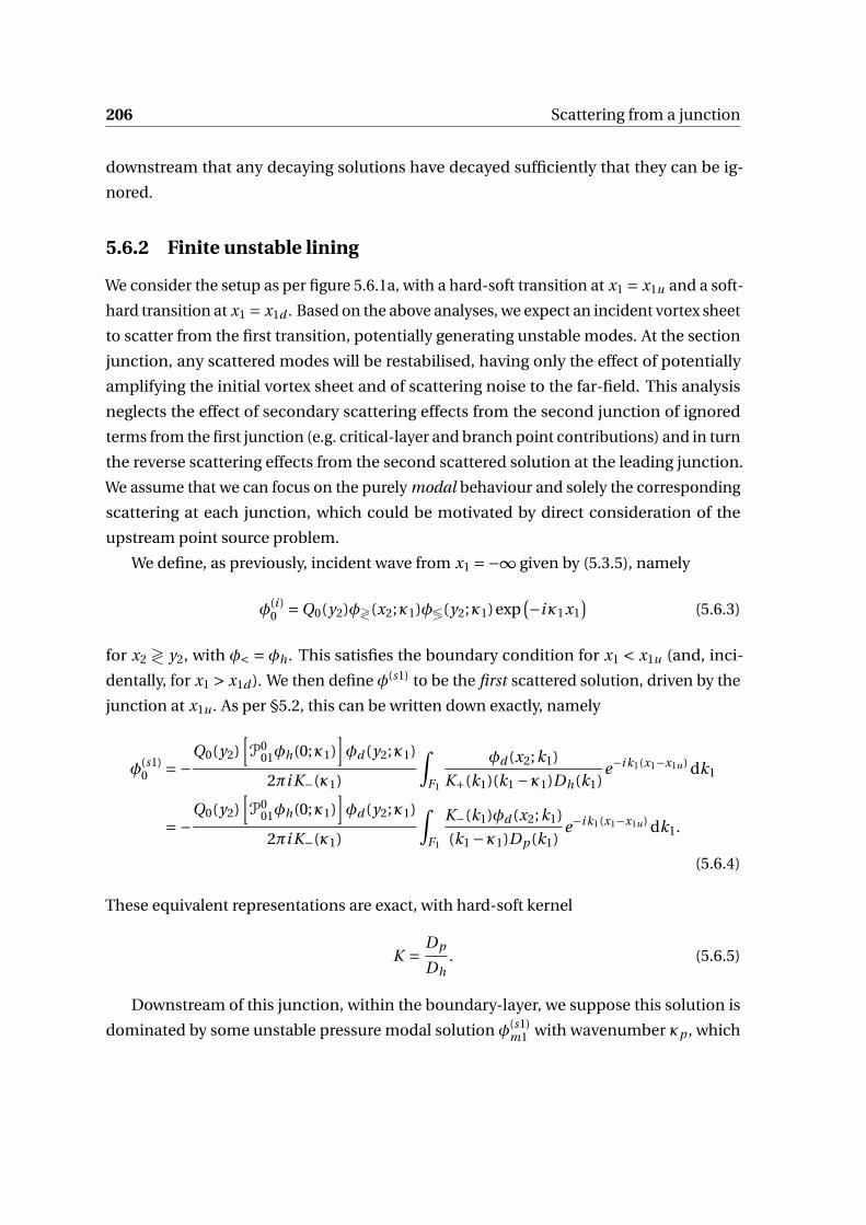
206 Scattering from a junction

downstream that any decaying solutions have decayed sufficiently that they can be ig-

nored.

5.6.2 Finite unstable lining

We consider the setup as per figure 5.6.1a, with a hard-soft transition at x1 = x1u and a soft-

hard transition at x1 = x1d . Based on the above analyses, we expect an incident vortex sheet

to scatter from the first transition, potentially generating unstable modes. At the section

junction, any scattered modes will be restabilised, having only the effect of potentially

amplifying the initial vortex sheet and of scattering noise to the far-field. This analysis

neglects the effect of secondary scattering effects from the second junction of ignored

terms from the first junction (e.g. critical-layer and branch point contributions) and in turn

the reverse scattering effects from the second scattered solution at the leading junction.

We assume that we can focus on the purely modal behaviour and solely the corresponding

scattering at each junction, which could be motivated by direct consideration of the

upstream point source problem.

We define, as previously, incident wave from x1 =−∞ given by (5.3.5), namely

φ(i )0 =Q0(y2)φ≷(x2;κ1)φ≶(y2;κ1)exp

(−iκ1x1)

(5.6.3)

for x2 ≷ y2, with φ< = φh . This satisfies the boundary condition for x1 < x1u (and, inci-

dentally, for x1 > x1d ). We then define φ(s1) to be the first scattered solution, driven by the

junction at x1u . As per §5.2, this can be written down exactly, namely

φ(s1)0 =−

Q0(y2)[P0

01φh(0;κ1)]φd (y2;κ1)

2πi K−(κ1)

∫F1

φd (x2;k1)

K+(k1)(k1 −κ1)Dh(k1)e−i k1(x1−x1u ) dk1

=−Q0(y2)

[P0

01φh(0;κ1)]φd (y2;κ1)

2πi K−(κ1)

∫F1

K−(k1)φd (x2;k1)

(k1 −κ1)Dp (k1)e−i k1(x1−x1u ) dk1.

(5.6.4)

These equivalent representations are exact, with hard-soft kernel

K = Dp

Dh. (5.6.5)

Downstream of this junction, within the boundary-layer, we suppose this solution is

dominated by some unstable pressure modal solution φ(s1)m1 with wavenumber κp , which

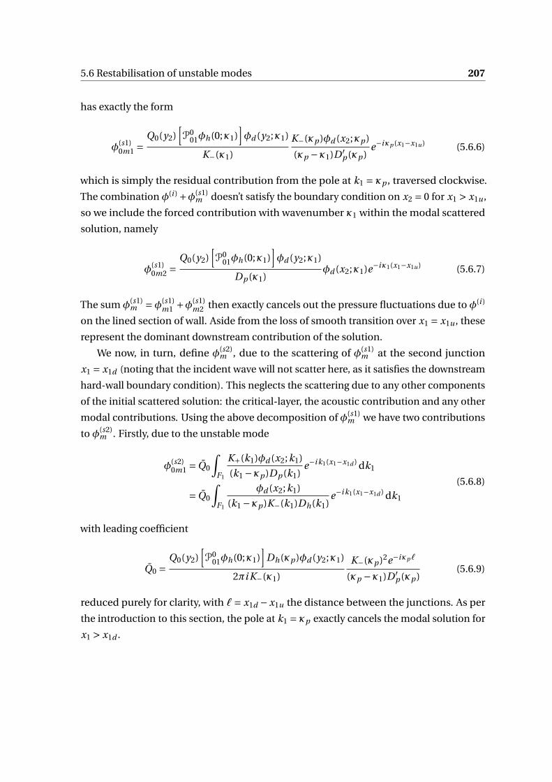
5.6 Restabilisation of unstable modes 207

has exactly the form

φ(s1)0m1 =

Q0(y2)[P0

01φh(0;κ1)]φd (y2;κ1)

K−(κ1)

K−(κp )φd (x2;κp )

(κp −κ1)D ′p (κp )

e−iκp (x1−x1u ) (5.6.6)

which is simply the residual contribution from the pole at k1 = κp , traversed clockwise.

The combination φ(i ) +φ(s1)m doesn’t satisfy the boundary condition on x2 = 0 for x1 > x1u ,

so we include the forced contribution with wavenumber κ1 within the modal scattered

solution, namely

φ(s1)0m2 =

Q0(y2)[P0

01φh(0;κ1)]φd (y2;κ1)

Dp (κ1)φd (x2;κ1)e−iκ1(x1−x1u ) (5.6.7)

The sum φ(s1)m =φ(s1)

m1 +φ(s1)m2 then exactly cancels out the pressure fluctuations due to φ(i )

on the lined section of wall. Aside from the loss of smooth transition over x1 = x1u , these

represent the dominant downstream contribution of the solution.

We now, in turn, define φ(s2)m , due to the scattering of φ(s1)

m at the second junction

x1 = x1d (noting that the incident wave will not scatter here, as it satisfies the downstream

hard-wall boundary condition). This neglects the scattering due to any other components

of the initial scattered solution: the critical-layer, the acoustic contribution and any other

modal contributions. Using the above decomposition of φ(s1)m we have two contributions

to φ(s2)m . Firstly, due to the unstable mode

φ(s2)0m1 = Q0

∫F1

K+(k1)φd (x2;k1)

(k1 −κp )Dp (k1)e−i k1(x1−x1d ) dk1

= Q0

∫F1

φd (x2;k1)

(k1 −κp )K−(k1)Dh(k1)e−i k1(x1−x1d ) dk1

(5.6.8)

with leading coefficient

Q0 =Q0(y2)

[P0

01φh(0;κ1)]

Dh(κp )φd (y2;κ1)

2πi K−(κ1)

K−(κp )2e−iκpℓ

(κp −κ1)D ′p (κp )

(5.6.9)

reduced purely for clarity, with ℓ= x1d −x1u the distance between the junctions. As per

the introduction to this section, the pole at k1 = κp exactly cancels the modal solution for

x1 > x1d .

208 Scattering from a junction

The second contribution, due to the forcing solution, is

φ(s2)0m2 =

Q0(y2)[P0

01φh(0;κ1)]φd (y2;κ1)

2πi K+(κ1)e−iκ1ℓ

∫F1

K+(k1)φd (x2;k1)

(k1 −κ1)Dp (k1)e−i k1(x1−x1d ) dk1

=Q0(y2)

[P0

01φh(0;κ1)]φd (y2;κ1)

2πi K+(κ1)e−iκ1ℓ

∫F1

φd (x2;k1)

(k1 −κ1)K−(k1)Dh(k1)e−i k1(x1−x1d ) dk1

(5.6.10)

Again, the pole at k1 = κ1 exactly cancels out the solution for x1u < x1 < x1d . In both

cases, the Wiener-Hopf kernel is the reciprocal of the hard-soft kernel, and as such the

splitfunctions are the reciprocal of what would normally be used. Far downstream of the

second junction, only the incident wave persists (assuming the decay of any critical-layer

and acoustic contributions). The unstable mode doesn’t propagate beyond the section

of lining, and it therefore appears to have no strong effect on the solution. However, if

the desire is to control far-field noise, then its contribution is noticeable. We have three

scattering contributions computed: the scattering of the incident field off the first junction,

and the scattering of the two propagating fields off the second junction. The far-field

noise due to all three can be computed using the steepest descent method as previously.

Importantly, if Im(κu) > 0, for large ℓ we expect a large amplification of the scattered

solution.

The complete solution (up to the approximations made) is shown in figure 5.6.2, for

ℓ= 5. This is not sufficiently large for the critical-layer contribution from the first junction

to decay, but shows the broad accuracy of the method, including the dominance on

downstream scattering due to the unstable mode excited at the upstream junction. The

second plot, figure 5.6.2b shows the solution only due to the first scattering point, with

the excited modal contribution only shown between the junctions (−5 < x1 < 0).

Far-field evaluation directly generalises §4.3.1. Neglecting the scaling functions

Q0(y2)[P0

01φh(0;κ1)]φd (y2;κ1)

2πi, (5.6.11)

common to all terms, outwith the boundary-layer we have an integral of the form∫F1

(I (s1)(k1)+ I (s2)

1 (k1)+ I (s2)2 (k1)

)e−i k1x1−γ∞x2 (5.6.12)

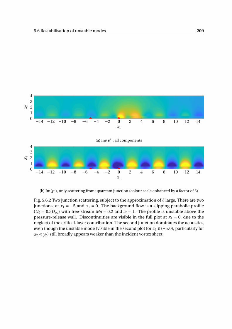
5.6 Restabilisation of unstable modes 209

−14 −12 −10 −8 −6 −4 −2 0 2 4 6 8 10 12 1401234

x1

x 2

(a) Im(p ′), all components

−14 −12 −10 −8 −6 −4 −2 0 2 4 6 8 10 12 1401234

x1

x 2

(b) Im(p ′), only scattering from upstream junction (colour scale enhanced by a factor of 5)

Fig. 5.6.2 Two junction scattering, subject to the approximation of ℓ large. There are twojunctions, at x1 = −5 and x1 = 0. The background flow is a slipping parabolic profile(U0 = 0.3U∞) with free-stream Ma = 0.2 and ω = 1. The profile is unstable above thepressure-release wall. Discontinuities are visible in the full plot at x1 = 0, due to theneglect of the critical-layer contribution. The second junction dominates the acoustics,even though the unstable mode (visible in the second plot for x1 ∈ (−5,0), particularly forx2 < y2) still broadly appears weaker than the incident vortex sheet.

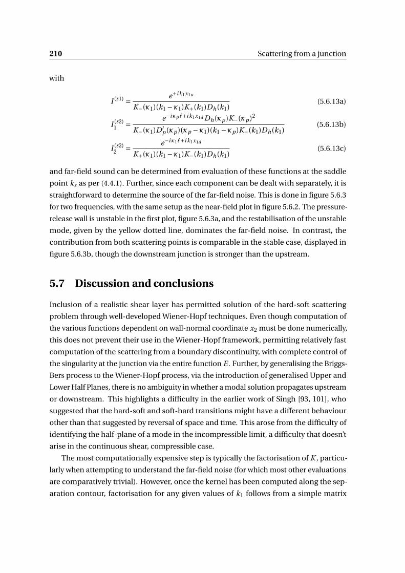
210 Scattering from a junction

with

I (s1) = e+i k1x1u

K−(κ1)(k1 −κ1)K+(k1)Dh(k1)(5.6.13a)

I (s2)1 = e−iκpℓ+i k1x1d Dh(κp )K−(κp )2

K−(κ1)D ′p (κp )(κp −κ1)(k1 −κp )K−(k1)Dh(k1)

(5.6.13b)

I (s2)2 = e−iκ1ℓ+i k1x1d

K+(κ1)(k1 −κ1)K−(k1)Dh(k1)(5.6.13c)

and far-field sound can be determined from evaluation of these functions at the saddle

point ks as per (4.4.1). Further, since each component can be dealt with separately, it is

straightforward to determine the source of the far-field noise. This is done in figure 5.6.3

for two frequencies, with the same setup as the near-field plot in figure 5.6.2. The pressure-

release wall is unstable in the first plot, figure 5.6.3a, and the restabilisation of the unstable

mode, given by the yellow dotted line, dominates the far-field noise. In contrast, the

contribution from both scattering points is comparable in the stable case, displayed in

figure 5.6.3b, though the downstream junction is stronger than the upstream.

5.7 Discussion and conclusions

Inclusion of a realistic shear layer has permitted solution of the hard-soft scattering

problem through well-developed Wiener-Hopf techniques. Even though computation of

the various functions dependent on wall-normal coordinate x2 must be done numerically,

this does not prevent their use in the Wiener-Hopf framework, permitting relatively fast

computation of the scattering from a boundary discontinuity, with complete control of

the singularity at the junction via the entire function E . Further, by generalising the Briggs-

Bers process to the Wiener-Hopf process, via the introduction of generalised Upper and

Lower Half Planes, there is no ambiguity in whether a modal solution propagates upstream

or downstream. This highlights a difficulty in the earlier work of Singh [93, 101], who

suggested that the hard-soft and soft-hard transitions might have a different behaviour

other than that suggested by reversal of space and time. This arose from the difficulty of

identifying the half-plane of a mode in the incompressible limit, a difficulty that doesn’t

arise in the continuous shear, compressible case.

The most computationally expensive step is typically the factorisation of K , particu-

larly when attempting to understand the far-field noise (for which most other evaluations

are comparatively trivial). However, once the kernel has been computed along the sep-

aration contour, factorisation for any given values of k1 follows from a simple matrix

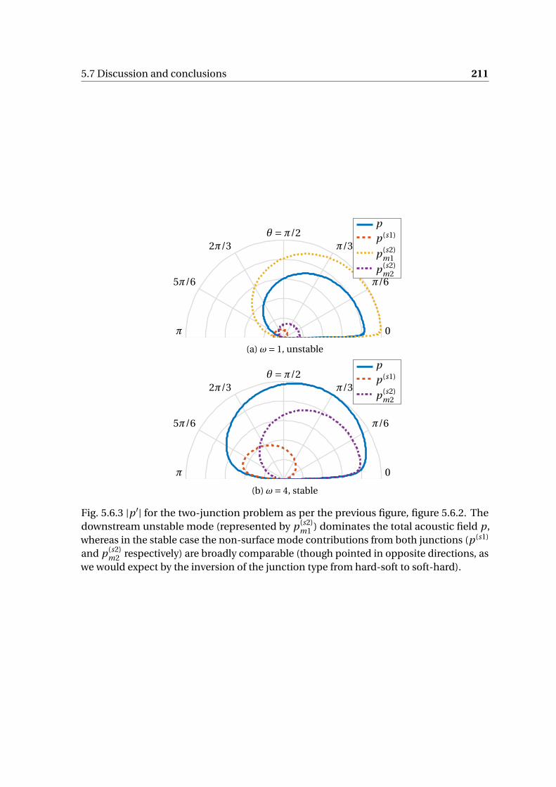
5.7 Discussion and conclusions 211

0

π/6

π/3θ =π/2

π

5π/6

2π/3

p

p(s1)

p(s2)m1

p(s2)m2

(a) ω= 1, unstable

0

π/6

π/3θ =π/2

π

5π/6

2π/3

p

p(s1)

p(s2)m2

(b) ω= 4, stable

Fig. 5.6.3 |p ′| for the two-junction problem as per the previous figure, figure 5.6.2. Thedownstream unstable mode (represented by p(s2)

m1 ) dominates the total acoustic field p,whereas in the stable case the non-surface mode contributions from both junctions (p(s1)

and p(s2)m2 respectively) are broadly comparable (though pointed in opposite directions, as

we would expect by the inversion of the junction type from hard-soft to soft-hard).

212 Scattering from a junction

multiplication, and is thus relatively rapid. Therefore, once the factorisations have been

computed once, it is straightforward to determine on any inversion contours of interest.

In fact, since the x2-dependence of the scattered solution depends on the source location

only in amplitude, if regarding this vortex sheet scattering as a Green’s function, integration

for generic vorticity distribution is straightforward to generalise, without re-evaluation

of K± or φd (x2;k1) being required, which will be exploited in the next chapter when the

slightly more difficult trailing-edge scattering problem is tackled.

Previous work [89] has noted that the hard-soft scattering problem is essentially equiva-

lent to the trailing-edge scattering problem. Whilst the distortion of radiation by boundary-

layer shear has an effect on the radiation direction from the junction, this result remains

true in this case, up to the caveat that the background profile is symmetric in the trailing-

edge case, which will be discussed in the next chapter §6. This is most obvious from

the sin(θ/2)-type profile seen for low Mach numbers and long acoustic wavelengths, for

which the effect of boundary-layer shear on radiation is least. This is exactly the pressure-

scattering profile that would be expected at the trailing-edge of a hard-plate, and there are

clear symmetry reasons why that should be the case as outlined below.

The most difficult step, mathematically, is determination of some function which,

for large k1, behaves as the Wiener-Hopf kernel, but which can be factorised analytically.

Typically, inspired by Noble [79] and Veitch [109], it is possible to compare behaviour with

some product of complex powers of (k1−kb±). Indeed, this is the approach taken by Singh

[101]. This appears to provide an analytic result in this case, in fact exactly this product,

though it suggests far-field sound behaving like (x1 + i x2)α where α is non-real, which

is curious on physical grounds. This is an artifact of the incompressible limit, however,

for which the two acoustic branch points “pinch” together. This removes the possibility

of defining a Wiener-Hopf strip, in this limit, and therefore the whole process breaks

down. However, in this chapter we considered the solution for finite c0 and allowed it to

be large. As shown by figure 5.4.6, we get exactly the sin(θ/2) dependence that we would

expect from a trailing-edge, which is simply the symmetric extension of the hard-soft

problem. Essentially, the complex powers in the far-field kernel asymptotic approximation

are cancelled out when the numerical factorisation is computed, and do not persist into

the final solution, though this numerical factorisation can only be computed when c0 is

finite (or under some other regularisation, e.g. k3 non-zero).

The final section highlights how some essentially invisible surface mode can lead to a

strong source of far-field acoustic noise. This highlights the importance of understanding

the hydrodynamic forcing solution within the boundary-layer in the computation of the

resulting far-field sound, which relates to the central thrust of this thesis, in understanding

5.7 Discussion and conclusions 213

how turbulence displacement within the boundary-layer can affect far-field noise. This is

more explicitly evaluated in the next chapter §6, which considers scattering of a similar

vortex sheet, and more generalised solutions, from a trailing-edge, through development

of the methods in this chapter.

Chapter 6

Scattering from a sharp trailing-edge

Extending the analysis from the previous chapter, the scattering of a vortex sheet (and,

in turn, more general vorticity distributions) from a sharp trailing-edge is computed.

Previous models are enhanced by the inclusion of a background flow profile, which

further allows consideration of asymmetric profiles (potentially with different free-stream

velocities above and below the plate), and scattering from a lined plate.

6.1 Introduction

The problem of scattering from a trailing-edge, with the inclusion of background shear,

has motivated this work from the outset. As outlined in the introduction, a variety of noise

control methods exist which, through either the deflection of turbulence, or the shielding

of the hard, scattering surface of the aerofoil, reduce surface pressure fluctuations near the

trailing-edge, which in turn (either theoretically [3, 106] or, less frequently, experimentally

measured [24]) reduces the far-field noise.

Due to both its importance in understanding the noise of sharp edges, and its mathe-

matical elegance, the trailing-edge scattering problem is well-studied, with a variety of

different models suggested for dealing with it. Most experimental work predicts far-field

noise through the utilisation of an acoustic analogy, for example that of Ffowcs Williams

and Hawking [35], which allows known acoustic perturbations in some control region

to be propagated to the far-field, a similar approach to that used by Amiet [5]. These

methods are useful numerically and experimentally, the former to overcome difficulties

with propagating waves near the edge of computational domains, the latter to remove the

need to directly measure far-field noise, instead utilising the measurable surface pressure

spectrum. A variety of mathematical models exist, including varying degrees of physical

complexity, for example that of Howe [56] and Ffowcs Williams and Hall [34].

216 Scattering from a sharp trailing-edge

The fundamental mechanism through which vorticity is converted into far-field noise

is the (unsteady) Kutta condition [31] and is well-understood. It generalises the well-

understood classical Kutta-Joukowsky hypothesis, which brings together the effect of

viscosity on a steady flow about an aerofoil into a single condition at the trailing-edge,

allowing unique choice of the circulation about the aerofoil. In unsteady aerodynamics it

has similarly come to mean the removal of a velocity singularity at some distinguished

point, typically a sharp trailing-edge or corner, or (as we saw in the previous chapter) at

a boundary discontinuity. The Wiener-Hopf procedure gives the desired control of this

tip singularity, and the analysis in the previous extension can be extended, incorporating

background asymmetry and upstream lining, though if the upstream boundary is different

on either side of the (flat) upstream plate, standard methods are typically unavailable.

This analysis makes the simplifying assumption, previously made throughout this

work, that we are considering linearised perturbations to a parallel mean background flow.

This is problematic in two obvious ways: firstly it doesn’t allow the mean flow to develop

rapidly as it passes the trailing-edge, as we assume it remains frozen as it passes over the

trailing-edge. It therefore cannot satisfy realistic non-slip conditions upstream and be a

developing wake downstream of the trailing-edge, and as such we generally focus on the

case considered by Schuster [96] with the background slip velocity, U0, being non-zero,

in an attempt to model both the upstream and downstream mean flow. It is possible

to develop a theory in which the background flow is developing on some slow scale,

which, locally to the trailing-edge, result in the same perturbation equations as being

solved in this work. The parallel flow assumption also somewhat limits the geometries

that can be considered, with any (no-penetration) conditions needing to be aligned

with the background flow. This essentially limits consideration to flat plate geometries,

though interesting trailing-edge geometries could be considered, for example serrations

[7]. Again, through consideration of perturbations to slowly developing background flow

this assumption can be relaxed somewhat to include more realistic aerofoil geometries

[11].

This chapter begins by solving the scattering of a upstream gust by a sharp trailing-

edge, on either a hard, or a pressure-release or a lined aerofoil. This idealised vortex sheet

is then associated with vortical perturbations in the wake, and the scattering of a more

general convected disturbance is generated in §6.3. This is then related to the central

hypotheses of this work: the mechanism behind which deflection of turbulence reduces

surface pressure, and in turn the transfer of this disturbance to far-field noise.

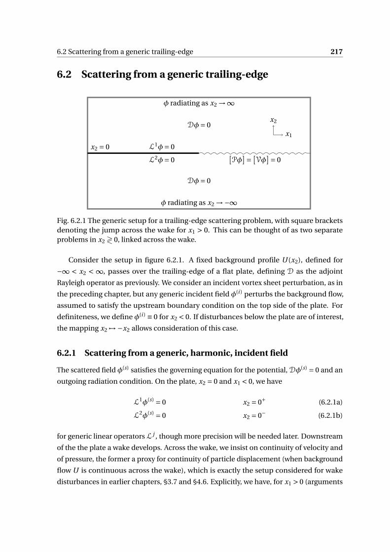
6.2 Scattering from a generic trailing-edge 217

6.2 Scattering from a generic trailing-edge

x2 = 0

x2

x1

Dφ= 0

Dφ= 0

L1φ= 0

L2φ= 0[Pφ

]= [Vφ

]= 0

φ radiating as x2 →∞

φ radiating as x2 →−∞

Fig. 6.2.1 The generic setup for a trailing-edge scattering problem, with square bracketsdenoting the jump across the wake for x1 > 0. This can be thought of as two separateproblems in x2 ≷ 0, linked across the wake.

Consider the setup in figure 6.2.1. A fixed background profile U (x2), defined for

−∞ < x2 < ∞, passes over the trailing-edge of a flat plate, defining D as the adjoint

Rayleigh operator as previously. We consider an incident vortex sheet perturbation, as in

the preceding chapter, but any generic incident field φ(i ) perturbs the background flow,

assumed to satisfy the upstream boundary condition on the top side of the plate. For

definiteness, we define φ(i ) ≡ 0 for x2 < 0. If disturbances below the plate are of interest,

the mapping x2 7→ −x2 allows consideration of this case.

6.2.1 Scattering from a generic, harmonic, incident field

The scattered field φ(s) satisfies the governing equation for the potential, Dφ(s) = 0 and an

outgoing radiation condition. On the plate, x2 = 0 and x1 < 0, we have

L1φ(s) = 0 x2 = 0+ (6.2.1a)

L2φ(s) = 0 x2 = 0− (6.2.1b)

for generic linear operators L j , though more precision will be needed later. Downstream

of the the plate a wake develops. Across the wake, we insist on continuity of velocity and

of pressure, the former a proxy for continuity of particle displacement (when background

flow U is continuous across the wake), which is exactly the setup considered for wake

disturbances in earlier chapters, §3.7 and §4.6. Explicitly, we have, for x1 > 0 (arguments

218 Scattering from a sharp trailing-edge

indicating location of x2 evaluation)

P0+φ(s)(0+)−P0−φ(s)(0−) =−P0+φ(i )(0+) (6.2.2a)

V0+φ(s)(0+)−V0−φ(s)(0−) =−V0+φ(i )(0+). (6.2.2b)

As in the previous chapter, we can take half-range transformations of these conditions.

For clarity, we define Φ1 to be the Fourier transform of φ(s), evaluated at x2 = 0+, and

similarlyΦ2 ofφ(s) evaluated at x2 = 0−. Further,P1,2 =P0± , and the same forV. Essentially

we reduce the problem into two regions: 1 denoting x2 > 0 and 2 denoting x2 < 0, linked

across the wake. Taking half-range transforms (and assuming time-harmonic dependence)

gives

L101Φ

−1 = 0 (6.2.3a)

L201Φ

−2 = 0 (6.2.3b)

P101Φ

+1 −P2

01Φ+2 =−I+p (6.2.3c)

V101Φ

+1 −V2

01Φ+2 =−I+v (6.2.3d)

with Ip and Iv respectively the Fourier transformed pressure and wall-normal velocity

perturbations due to the incident fieldφ(i ). Finally, we note the radiation condition implies

the solution decays as x2 →±∞. Defining φ1,2 to be the decaying solution as x2 →±∞,

normalised so that φ1,2 → exp(∓γ±x2) as per §4.6, we must have

φ(s) = A1(k1)φ1(x2;k1) x2 > 0

A2(k1)φ2(x2;k1) x2 < 0.(6.2.4)

and soΦ j = A j (k1)φ j (0;k1) for j = 1,2.

Using (6.2.3), we find four equations for A j in terms of unknown functions, namely

A1L101φ1 =L1

01Φ+1 ≡ B+

1 , (6.2.5a)

A2L201φ2 =L2

01Φ+2 ≡ B+

2 , (6.2.5b)

A1P101φ1 − A2P

201φ2 =P1

01Φ−1 −P2

01Φ−2 − I+p ≡C−

p − I+p , (6.2.5c)

A1V101φ1 − A2V

201φ2 =V1

01Φ−1 −V2

01Φ−2 − I+v ≡C−

v − I+v . (6.2.5d)

All φ j are evaluated at x2 = 0, above or below the plate or wake as appropriate.

We have four equations and six unknowns: the coefficients A1,2, the downstream ex-

tension of the boundary conditions B+1,2, and the pressure and velocity jumps in scattered

6.2 Scattering from a generic trailing-edge 219

solution across the plate, C−p,v . Eliminating A1,2 gives two coupled Wiener-Hopf equations,

namely

B+1

P101φ1

L101φ1

−B+2

P201φ2

L201φ2

=C−p − I+p , (6.2.6a)

B+1

V101φ1

L101φ1

−B+2

V201φ2

L201φ2

=C−v − I+v . (6.2.6b)

Whilst this equation can be written in the form KB+ = C−− I+, a matrix equation which

exactly extends (5.2.11), factorising the matrix K is non-trivial. We therefore make the

assumption that the upstream boundary condition corresponds to some impedance

condition LZ , with Z the same on both sides of the plate. In the asymmetric case, this

is not setting L1 = L2, since the shear (and therefore P) may be different for x2 = 0±.

Explicitly,

LZ01 = iωZV01 −C0P01. (6.2.7)

If we impose this boundary condition above and below the plate, then trivially the

quantity LZφ is continuous across the plate, vanishing on both sides. Further, since L is a

linear combination of pressure and (wall-normal) velocity operators, and both these are

continuous across the wake, we end up with the strong condition that

L101Φ1 −L2

01Φ2 = 0. (6.2.8)

Via (6.2.5a) and (6.2.5b), this is simply the condition that B+1 = B+

2 . A similar relationship

could be written down linking C−p and C−

v , but it is worth noting that now we have a

decoupled Wiener-Hopf system, namely(P1

01φ1

L101φ1

− P201φ2

L201φ2

)B+

1 =C−p − I+p . (6.2.9)

This is appropriate for Z = 0, including the hard-wall case, but it is trivial in the case

Z = 0 and the alternative representation with P→V should be used. The Wiener-Hopf

kernel can be simplified:

K =(P1

01φ1

L101φ1

− P201φ2

L201φ2

)= iωZ

P101φ1V

201φ2 −V1

01φ1P201φ2

L101φ1L

201φ2

. (6.2.10)

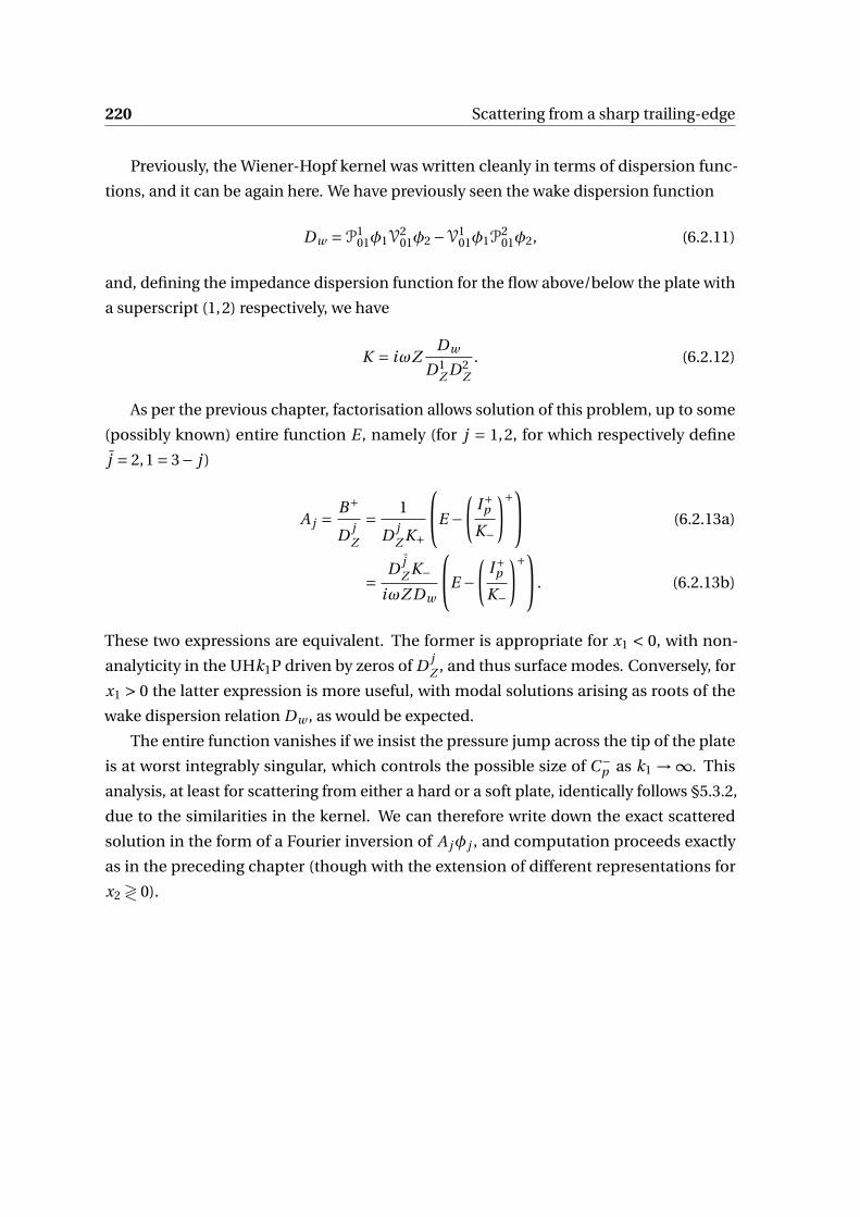
220 Scattering from a sharp trailing-edge

Previously, the Wiener-Hopf kernel was written cleanly in terms of dispersion func-

tions, and it can be again here. We have previously seen the wake dispersion function

Dw =P101φ1V

201φ2 −V1

01φ1P201φ2, (6.2.11)

and, defining the impedance dispersion function for the flow above/below the plate with

a superscript (1,2) respectively, we have

K = iωZDw

D1Z D2

Z

. (6.2.12)

As per the previous chapter, factorisation allows solution of this problem, up to some

(possibly known) entire function E , namely (for j = 1,2, for which respectively define

j = 2,1 = 3− j )

A j = B+

D jZ

= 1

D jZ K+

E −(

I+pK−

)+ (6.2.13a)

= D jZ K−

iωZ Dw

E −(

I+pK−

)+ . (6.2.13b)

These two expressions are equivalent. The former is appropriate for x1 < 0, with non-

analyticity in the UHk1P driven by zeros of D jZ , and thus surface modes. Conversely, for

x1 > 0 the latter expression is more useful, with modal solutions arising as roots of the

wake dispersion relation Dw , as would be expected.

The entire function vanishes if we insist the pressure jump across the tip of the plate

is at worst integrably singular, which controls the possible size of C−p as k1 →∞. This

analysis, at least for scattering from either a hard or a soft plate, identically follows §5.3.2,

due to the similarities in the kernel. We can therefore write down the exact scattered

solution in the form of a Fourier inversion of A jφ j , and computation proceeds exactly

as in the preceding chapter (though with the extension of different representations for

x2 ≷ 0).

6.2 Scattering from a generic trailing-edge 221

6.2.2 The Green’s function: incident vortex sheet

We now consider explicitly the incident vortex sheet, either for its own merits or from

which to construct a more general vortical solution. As per §5, we therefore have

I+p =− 1

i (k1 −κ1)

[Q0(y2)φd (y2;κ1)P01φZ (0;κ1)

]≡− I0

i (k1 −κ1). (6.2.14)

We now define g = g (i )+g (s) to be exactly the solution to this problem, as a function of

y2 and κ(y2), so that g (i ) gives rise to the above forcing (with an explicit choice of Q0 noted

in §6.3 below). We have four exact representations for the scattered solution depending

on the signs of x1 and x2, namely

g (s) = I0(y2)

2πi K−(κ1)

∫F1

φ1(x2;k1)

D1Z (k1)

e−i k1x1

K+(k1)(k1 −κ1)dk1 x1 < 0, x2 > 0 (6.2.15a)

g (s) = I0(y2)

2πi K−(κ1)

∫F1

φ2(x2;k1)

D2Z (k1)

e−i k1x1

K+(k1)(k1 −κ1)dk1 x1 < 0, x2 < 0 (6.2.15b)

g (s) = I0(y2)

(2πi )(iωZ )K−(κ1)

∫F1

φ1(x2;k1)D2Z (k1)

Dw (k1)

K−(k1)e−i k1x1

(k1 −κ1)dk1 x1 > 0, x2 > 0 (6.2.15c)

g (s) = I0(y2)

(2πi )(iωZ )K−(κ1)

∫F1

φ2(x2;k1)D1Z (k1)

Dw (k1)

K−(k1)e−i k1x1

(k1 −κ1)dk1 x1 > 0, x2 < 0.

(6.2.15d)

F1 is, as usual, the causal deformation of the real axis as Im(ω) → 0 from below and, as

before, can be deformed to the relevant steepest descent contours (dependent on whether

x1 ≷ 0), picking up contributions from the poles of the dispersion relationships, and

from the forcing wavenumber κ1. Further, the branch cut along the critical-layer always

contributes for positive x1 (assuming U > 0 throughout). It is worth being explicit about

this contribution.

Let the zeros of D1Z be labelled κ1±

Z j , with N 1+Z in the gUHk1P and N 1−

Z in the gLHK1P,

so that j runs from 1 to N 1±Z repectively. Similarly, we label the zeros of D2

Z as κ2±Z j , and

the zeros of the wake κ±w j . Which half-plane they lie in is determined by the Briggs-Bers

procedure, and in practice defines the generalised half-planes. Explicitly picking up the

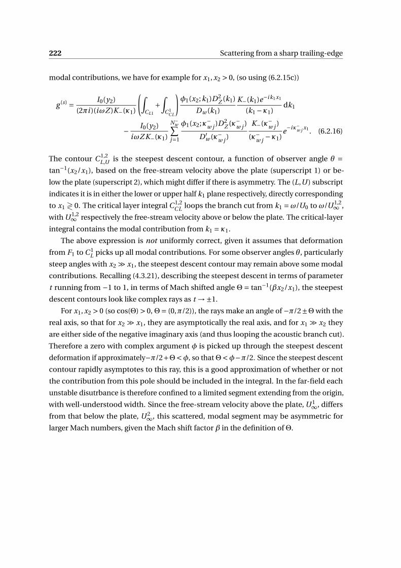
222 Scattering from a sharp trailing-edge

modal contributions, we have for example for x1, x2 > 0, (so using (6.2.15c))

g (s) = I0(y2)

(2πi )(iωZ )K−(κ1)

(∫CL1

+∫

C 1C L

)φ1(x2;k1)D2

Z (k1)

Dw (k1)

K−(k1)e−i k1x1

(k1 −κ1)dk1

− I0(y2)

iωZ K−(κ1)

N−w∑

j=1

φ1(x2;κ−w j )D2Z (κ−w j )

D ′w (κ−w j )

K−(κ−w j )

(κ−w j −κ1)e−iκ−w j x1 . (6.2.16)

The contour C 1,2L,U is the steepest descent contour, a function of observer angle θ =

tan−1(x2/x1), based on the free-stream velocity above the plate (superscript 1) or be-

low the plate (superscript 2), which might differ if there is asymmetry. The (L,U ) subscript

indicates it is in either the lower or upper half k1 plane respectively, directly corresponding

to x1 ≷ 0. The critical layer integral C 1,2C L loops the branch cut from k1 =ω/U0 to ω/U 1,2∞ ,

with U 1,2∞ respectively the free-stream velocity above or below the plate. The critical-layer

integral contains the modal contribution from k1 = κ1.

The above expression is not uniformly correct, given it assumes that deformation

from F1 to C 1L picks up all modal contributions. For some observer angles θ, particularly

steep angles with x2 ≫ x1, the steepest descent contour may remain above some modal

contributions. Recalling (4.3.21), describing the steepest descent in terms of parameter

t running from −1 to 1, in terms of Mach shifted angle Θ= tan−1(βx2/x1), the steepest

descent contours look like complex rays as t →±1.

For x1, x2 > 0 (so cos(Θ) > 0,Θ= (0,π/2)), the rays make an angle of −π/2±Θwith the

real axis, so that for x2 ≫ x1, they are asymptotically the real axis, and for x1 ≫ x2 they

are either side of the negative imaginary axis (and thus looping the acoustic branch cut).

Therefore a zero with complex argument φ is picked up through the steepest descent

deformation if approximately−π/2+Θ<φ, so thatΘ<φ−π/2. Since the steepest descent

contour rapidly asymptotes to this ray, this is a good approximation of whether or not

the contribution from this pole should be included in the integral. In the far-field each

unstable disutrbance is therefore confined to a limited segment extending from the origin,

with well-understood width. Since the free-stream velocity above the plate, U 1∞, differs

from that below the plate, U 2∞, this scattered, modal segment may be asymmetric for

larger Mach numbers, given the Mach shift factor β in the definition ofΘ.

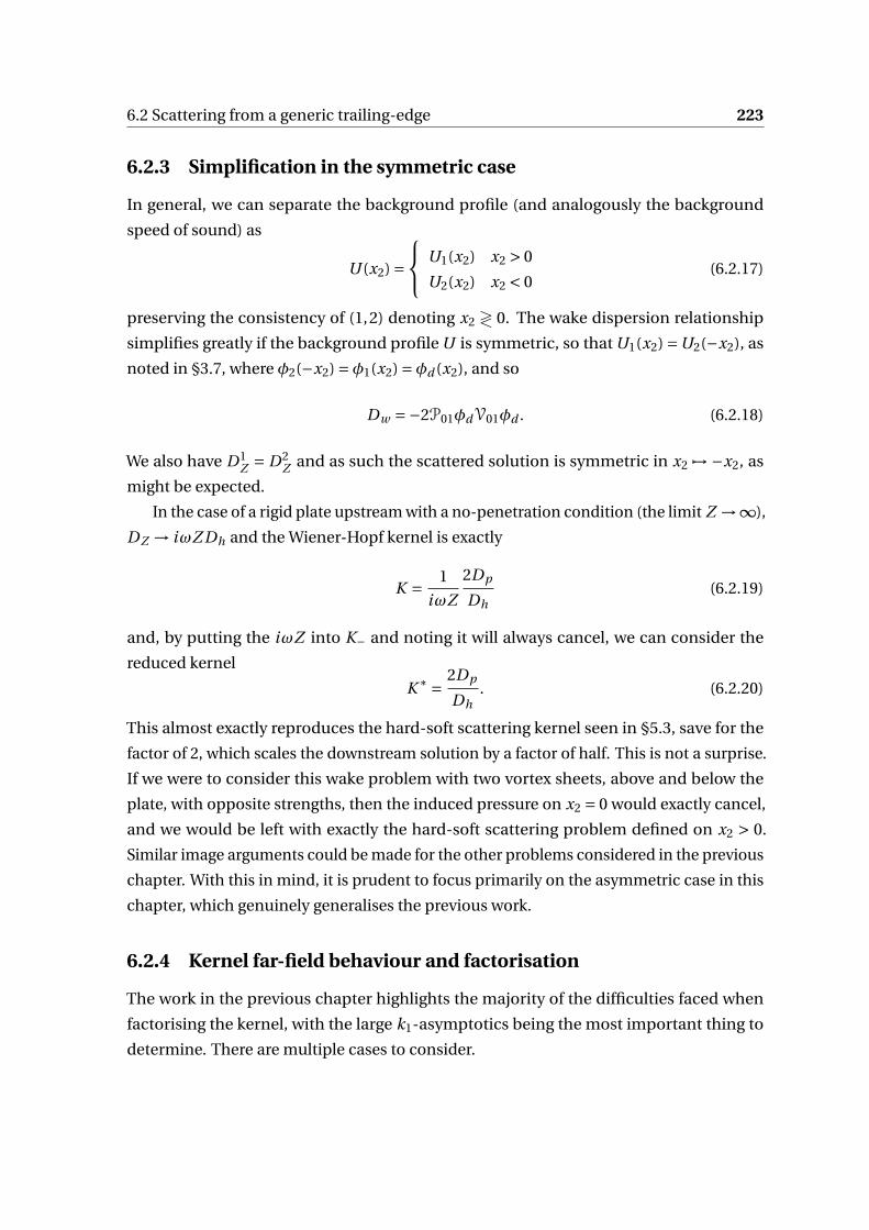
6.2 Scattering from a generic trailing-edge 223

6.2.3 Simplification in the symmetric case

In general, we can separate the background profile (and analogously the background

speed of sound) as

U (x2) = U1(x2) x2 > 0

U2(x2) x2 < 0(6.2.17)

preserving the consistency of (1,2) denoting x2 ≷ 0. The wake dispersion relationship

simplifies greatly if the background profile U is symmetric, so that U1(x2) =U2(−x2), as

noted in §3.7, where φ2(−x2) =φ1(x2) =φd (x2), and so

Dw =−2P01φdV01φd . (6.2.18)

We also have D1Z = D2

Z and as such the scattered solution is symmetric in x2 7→ −x2, as

might be expected.

In the case of a rigid plate upstream with a no-penetration condition (the limit Z →∞),

DZ → iωZ Dh and the Wiener-Hopf kernel is exactly

K = 1

iωZ

2Dp

Dh(6.2.19)

and, by putting the iωZ into K− and noting it will always cancel, we can consider the

reduced kernel

K ∗ = 2Dp

Dh. (6.2.20)

This almost exactly reproduces the hard-soft scattering kernel seen in §5.3, save for the

factor of 2, which scales the downstream solution by a factor of half. This is not a surprise.

If we were to consider this wake problem with two vortex sheets, above and below the

plate, with opposite strengths, then the induced pressure on x2 = 0 would exactly cancel,

and we would be left with exactly the hard-soft scattering problem defined on x2 > 0.

Similar image arguments could be made for the other problems considered in the previous

chapter. With this in mind, it is prudent to focus primarily on the asymmetric case in this

chapter, which genuinely generalises the previous work.

6.2.4 Kernel far-field behaviour and factorisation

The work in the previous chapter highlights the majority of the difficulties faced when

factorising the kernel, with the large k1-asymptotics being the most important thing to

determine. There are multiple cases to consider.

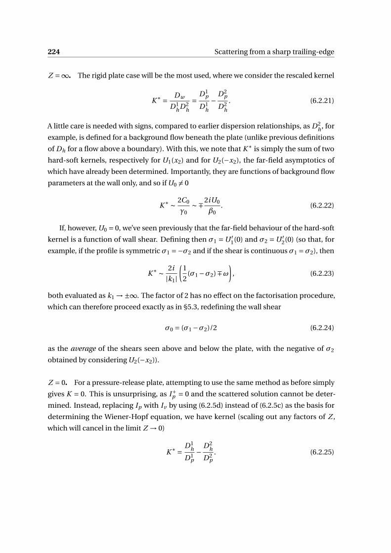
224 Scattering from a sharp trailing-edge

Z =∞. The rigid plate case will be the most used, where we consider the rescaled kernel

K ∗ = Dw

D1hD2

h

=D1

p

D1h

−D2

p

D2h

. (6.2.21)

A little care is needed with signs, compared to earlier dispersion relationships, as D2h , for

example, is defined for a background flow beneath the plate (unlike previous definitions

of Dh for a flow above a boundary). With this, we note that K ∗ is simply the sum of two

hard-soft kernels, respectively for U1(x2) and for U2(−x2), the far-field asymptotics of

which have already been determined. Importantly, they are functions of background flow

parameters at the wall only, and so if U0 = 0

K ∗ ∼ 2C0

γ0∼∓2iU0

β0. (6.2.22)

If, however, U0 = 0, we’ve seen previously that the far-field behaviour of the hard-soft

kernel is a function of wall shear. Defining then σ1 =U ′1(0) and σ2 =U ′

2(0) (so that, for

example, if the profile is symmetric σ1 =−σ2 and if the shear is continuous σ1 =σ2), then

K ∗ ∼ 2i

|k1|(

1

2(σ1 −σ2)∓ω

), (6.2.23)

both evaluated as k1 →±∞. The factor of 2 has no effect on the factorisation procedure,

which can therefore proceed exactly as in §5.3, redefining the wall shear

σ0 = (σ1 −σ2)/2 (6.2.24)

as the average of the shears seen above and below the plate, with the negative of σ2

obtained by considering U2(−x2)).

Z = 0. For a pressure-release plate, attempting to use the same method as before simply

gives K = 0. This is unsurprising, as I+p = 0 and the scattered solution cannot be deter-

mined. Instead, replacing Ip with Iv by using (6.2.5d) instead of (6.2.5c) as the basis for

determining the Wiener-Hopf equation, we have kernel (scaling out any factors of Z ,

which will cancel in the limit Z → 0)

K ∗ = D1h

D1p− D2

h

D2p

. (6.2.25)

6.2 Scattering from a generic trailing-edge 225

Since this is just the sum of the soft-hard kernels above and below the plate, the far-field

behaviour is straightforwardly

K ∗ ∼ 2γ0

C0∼±2iβ0

U0(6.2.26)

for U0 = 0, and

K ∗ ∼−i |k1|(

1

σ1 ∓ω+ 1

−σ2 ∓ω)=−2i |k1| σ0 ∓ω

(σ1 ∓ω)(−σ2 ∓ω)(6.2.27)

for U0 = 0, both in the limits k1 →±∞. σ0 is as defined above in (6.2.24).

We note in the symmetric case indicated above, the kernel is simply twice the hard-soft

kernel for the flow defined on x2 > 0, and there is essentially a reduction to the soft-hard

scattering problem. The symmetry could allow for more complicated flow profiles to be

solved as done by Rawlins [83], who considered a plate with different boundary conditions

above and below.

Z finite, non-zero, U0 = 0. If upstream impedance Z is finite and non-zero and the

background flow is slipping, for large k1 we have

D jZ ∼−C0D j

p (6.2.28)

The kernel therefore appears to vanish for large k1. However, we can be careful, and if we

note

Dw ∼ 2Dp Dh (6.2.29)

for large k1, where Dp and Dh are the large k1-behaviour which depends only on the

background flow velocity at x2 = 0. Hence,

K ∼ 2iωZ Dh

C 20 Dp

(6.2.30)

which does indeed vanish for large k1, though we have a stronger handle on the behaviour,

and we can write down

K ∼ 2iωZγ0

C 30

∼±2β0(iωZ )

U 30 |k1|2

. (6.2.31)

Z finite, non-zero, U0 = 0. Conversely, if U0 = 0, the dispersion function DZ ∼ iωDh .

This reduces to the problem considered above, up to some factors of iωZ , and

K ∼ 1

iωZ

2i

|k1|(σ0 ∓ω

)(6.2.32)

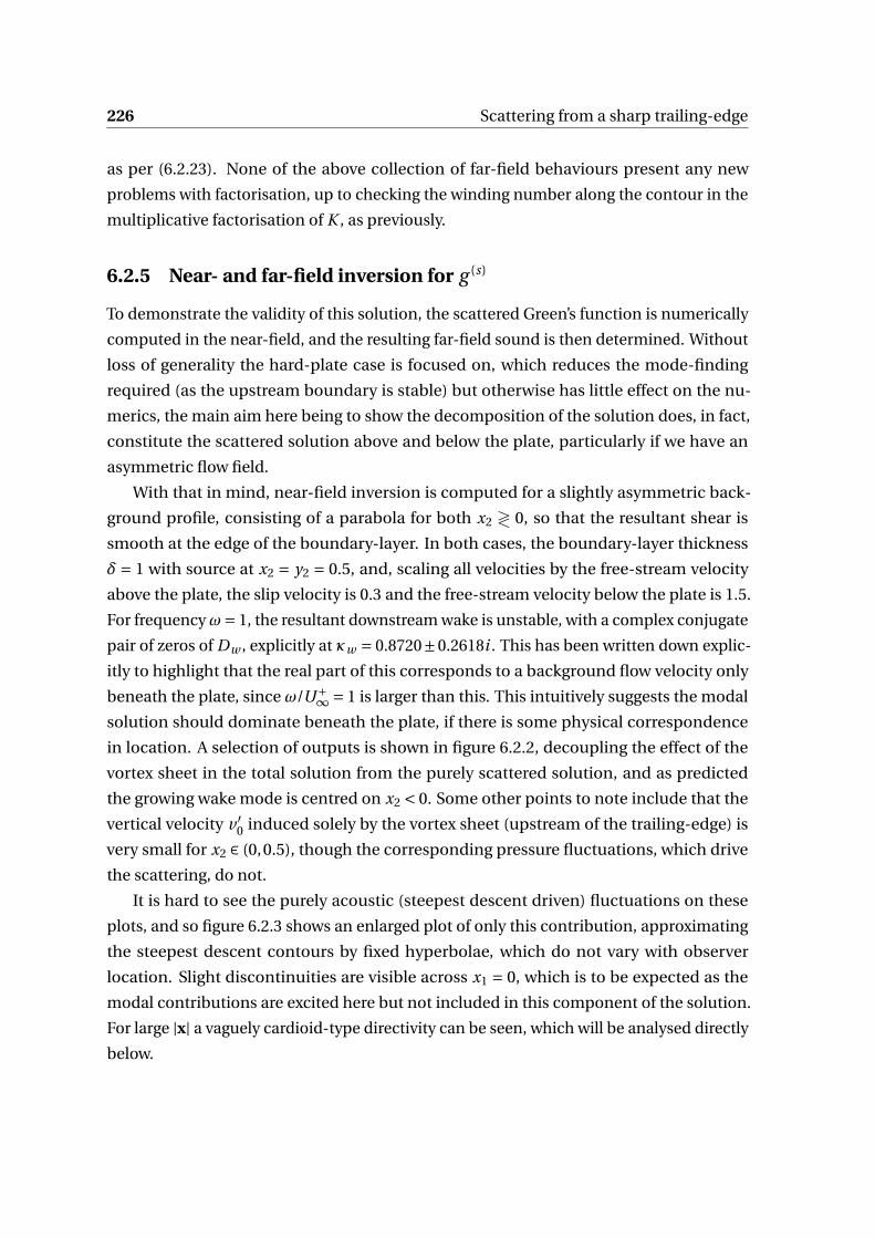
226 Scattering from a sharp trailing-edge

as per (6.2.23). None of the above collection of far-field behaviours present any new

problems with factorisation, up to checking the winding number along the contour in the

multiplicative factorisation of K , as previously.

6.2.5 Near- and far-field inversion for g (s)

To demonstrate the validity of this solution, the scattered Green’s function is numerically

computed in the near-field, and the resulting far-field sound is then determined. Without

loss of generality the hard-plate case is focused on, which reduces the mode-finding

required (as the upstream boundary is stable) but otherwise has little effect on the nu-

merics, the main aim here being to show the decomposition of the solution does, in fact,

constitute the scattered solution above and below the plate, particularly if we have an

asymmetric flow field.

With that in mind, near-field inversion is computed for a slightly asymmetric back-

ground profile, consisting of a parabola for both x2 ≷ 0, so that the resultant shear is

smooth at the edge of the boundary-layer. In both cases, the boundary-layer thickness

δ = 1 with source at x2 = y2 = 0.5, and, scaling all velocities by the free-stream velocity

above the plate, the slip velocity is 0.3 and the free-stream velocity below the plate is 1.5.

For frequencyω= 1, the resultant downstream wake is unstable, with a complex conjugate

pair of zeros of Dw , explicitly at κw = 0.8720±0.2618i . This has been written down explic-

itly to highlight that the real part of this corresponds to a background flow velocity only

beneath the plate, since ω/U+∞ = 1 is larger than this. This intuitively suggests the modal

solution should dominate beneath the plate, if there is some physical correspondence

in location. A selection of outputs is shown in figure 6.2.2, decoupling the effect of the

vortex sheet in the total solution from the purely scattered solution, and as predicted

the growing wake mode is centred on x2 < 0. Some other points to note include that the

vertical velocity v ′0 induced solely by the vortex sheet (upstream of the trailing-edge) is

very small for x2 ∈ (0,0.5), though the corresponding pressure fluctuations, which drive

the scattering, do not.

It is hard to see the purely acoustic (steepest descent driven) fluctuations on these

plots, and so figure 6.2.3 shows an enlarged plot of only this contribution, approximating

the steepest descent contours by fixed hyperbolae, which do not vary with observer

location. Slight discontinuities are visible across x1 = 0, which is to be expected as the

modal contributions are excited here but not included in this component of the solution.

For large |x| a vaguely cardioid-type directivity can be seen, which will be analysed directly

below.

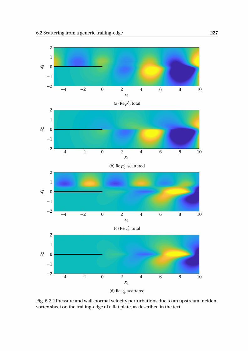
6.2 Scattering from a generic trailing-edge 227

−4 −2 0 2 4 6 8 10−2

−1

0

1

2

x1

x 2

(a) Re p ′0, total

−4 −2 0 2 4 6 8 10−2

−1

0

1

2

x1

x 2

(b) Re p ′0, scattered

−4 −2 0 2 4 6 8 10−2

−1

0

1

2

x1

x 2

(c) Re v ′0, total

−4 −2 0 2 4 6 8 10−2

−1

0

1

2

x1

x 2

(d) Re v ′0, scattered

Fig. 6.2.2 Pressure and wall-normal velocity perturbations due to an upstream incidentvortex sheet on the trailing-edge of a flat plate, as described in the text.

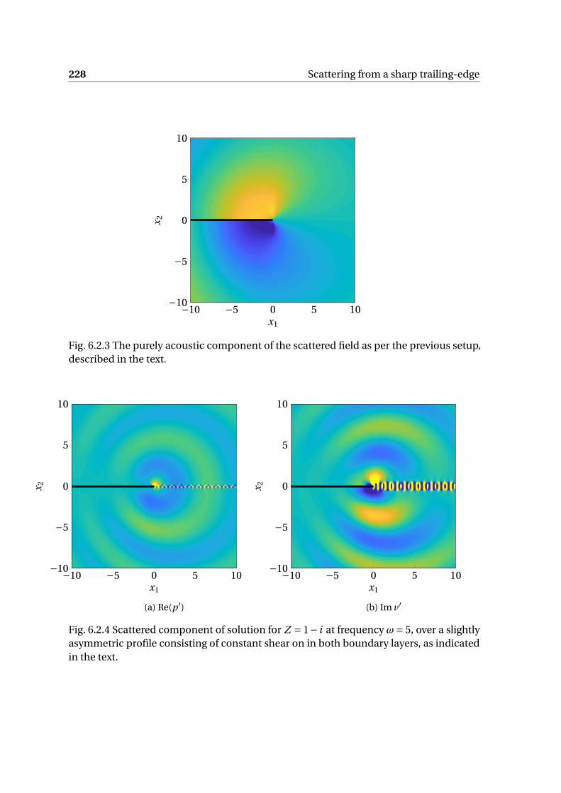
228 Scattering from a sharp trailing-edge

−10 −5 0 5 10−10

−5

0

5

10

x1

x 2

Fig. 6.2.3 The purely acoustic component of the scattered field as per the previous setup,described in the text.

−10 −5 0 5 10−10

−5

0

5

10

x1

x 2

(a) Re(p ′)

−10 −5 0 5 10−10

−5

0

5

10

x1

x 2

(b) Im v ′

Fig. 6.2.4 Scattered component of solution for Z = 1− i at frequency ω= 5, over a slightlyasymmetric profile consisting of constant shear on in both boundary layers, as indicatedin the text.

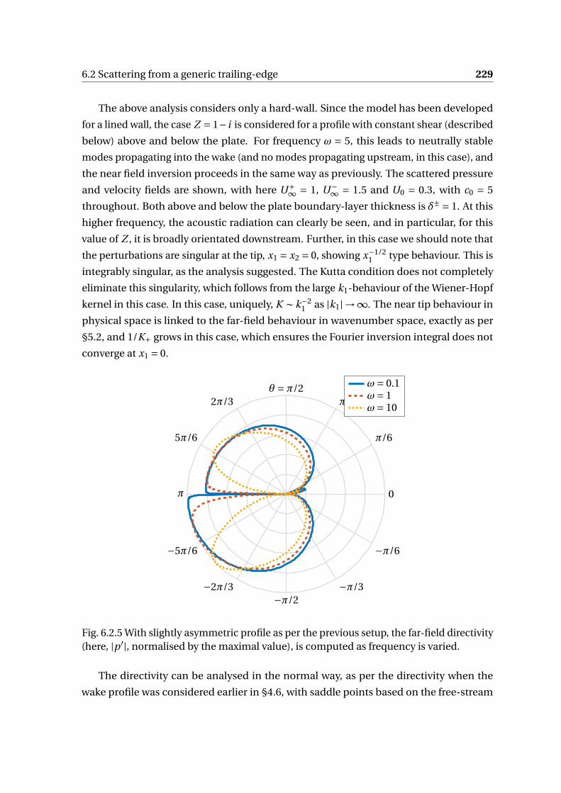
6.2 Scattering from a generic trailing-edge 229

The above analysis considers only a hard-wall. Since the model has been developed

for a lined wall, the case Z = 1−i is considered for a profile with constant shear (described

below) above and below the plate. For frequency ω = 5, this leads to neutrally stable

modes propagating into the wake (and no modes propagating upstream, in this case), and

the near field inversion proceeds in the same way as previously. The scattered pressure

and velocity fields are shown, with here U+∞ = 1, U−∞ = 1.5 and U0 = 0.3, with c0 = 5

throughout. Both above and below the plate boundary-layer thickness is δ± = 1. At this

higher frequency, the acoustic radiation can clearly be seen, and in particular, for this

value of Z , it is broadly orientated downstream. Further, in this case we should note that

the perturbations are singular at the tip, x1 = x2 = 0, showing x−1/21 type behaviour. This is

integrably singular, as the analysis suggested. The Kutta condition does not completely

eliminate this singularity, which follows from the large k1-behaviour of the Wiener-Hopf

kernel in this case. In this case, uniquely, K ∼ k−21 as |k1|→∞. The near tip behaviour in

physical space is linked to the far-field behaviour in wavenumber space, exactly as per

§5.2, and 1/K+ grows in this case, which ensures the Fourier inversion integral does not

converge at x1 = 0.

0

π/6

π/3θ =π/2

π

5π/6

2π/3

−π/6

−π/3−π/2

−5π/6

−2π/3

ω= 0.1ω= 1ω= 10

Fig. 6.2.5 With slightly asymmetric profile as per the previous setup, the far-field directivity(here, |p ′|, normalised by the maximal value), is computed as frequency is varied.

The directivity can be analysed in the normal way, as per the directivity when the

wake profile was considered earlier in §4.6, with saddle points based on the free-stream

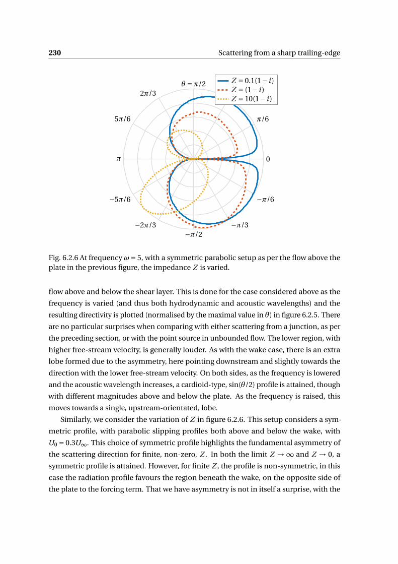
230 Scattering from a sharp trailing-edge

0

π/6

π/3θ =π/2

π

5π/6

2π/3

−π/6

−π/3−π/2

−5π/6

−2π/3

Z = 0.1(1− i )Z = (1− i )Z = 10(1− i )

Fig. 6.2.6 At frequency ω= 5, with a symmetric parabolic setup as per the flow above theplate in the previous figure, the impedance Z is varied.

flow above and below the shear layer. This is done for the case considered above as the

frequency is varied (and thus both hydrodynamic and acoustic wavelengths) and the

resulting directivity is plotted (normalised by the maximal value in θ) in figure 6.2.5. There

are no particular surprises when comparing with either scattering from a junction, as per

the preceding section, or with the point source in unbounded flow. The lower region, with

higher free-stream velocity, is generally louder. As with the wake case, there is an extra

lobe formed due to the asymmetry, here pointing downstream and slightly towards the

direction with the lower free-stream velocity. On both sides, as the frequency is lowered

and the acoustic wavelength increases, a cardioid-type, sin(θ/2) profile is attained, though

with different magnitudes above and below the plate. As the frequency is raised, this

moves towards a single, upstream-orientated, lobe.

Similarly, we consider the variation of Z in figure 6.2.6. This setup considers a sym-

metric profile, with parabolic slipping profiles both above and below the wake, with

U0 = 0.3U∞. This choice of symmetric profile highlights the fundamental asymmetry of

the scattering direction for finite, non-zero, Z . In both the limit Z → ∞ and Z → 0, a

symmetric profile is attained. However, for finite Z , the profile is non-symmetric, in this

case the radiation profile favours the region beneath the wake, on the opposite side of

the plate to the forcing term. That we have asymmetry is not in itself a surprise, with the

6.3 Distributed boundary-layer vorticity 231

symmetry in the hard-wall and pressure-release trailing-edge cases arising directly from

the reduction, in these cases, of the problem to either the hard-soft or soft-hard scattering

problem (up to a factor of two), with either symmetry of asymmetry in scattered pressure

across the wake.

For |Z | large, the solution tends towards the cardiod structure, orientated downstream,

as seen in figure 6.2.5. Conversely, for small |Z | this profile is flipped. As noted above,

this follows from the reduction of the scattering kernel to either the hard-soft or soft-hard

kernel, and the solution is essentially that discussed in detail in the previous chapter, §6.

Finally, the slight discontinuity across θ =π/2 must be noted. This is purely numerical, and

results from the slow decay of log(K /K f ), which causes difficulties in precise factorisation

of the Wiener-Hopf kernel.

A final caveat is that this plot and all preceding directivity plots, in both this chapter

and §5, show only the direction of radiated sound. For a concrete comparison of the

magnitude, it is important that we suitably normalise the forcing source term, which shall

be done carefully in the next section. This is important, for example when investigating

the importance of vortex sheet height y2, since this has very little effect on directivity but

a great effect on the magnitude of the radiating noise.

6.3 Distributed boundary-layer vorticity

Earlier, we defined g to be the Green’s function for the scattering problem, due to a vortex

sheet. Explictly, we require g to be the solution of

D†R0g0 = e−iκ1(y2)x1δ(xT −yT ) (6.3.1)

which fixes the scaling factor Q0. Recalling (2.3.15), the acoustics, or at least the generalised

potential φ which determines p ′ and v ′, is driven by some convected quantity

D†R0φ0 = e−iωx1/U (x2)F01(x2, x3) (6.3.2)

assuming a harmonic disturbance like e iωt , which fixes the streamwise dependence.

Therefore, if g0 satisfies the same boundary conditions as φ0, we can trivially write down

φ0 =∫

g0(x;yT )F01(yT )dyT (6.3.3)

which takes care of the forcing convected quantity.

232 Scattering from a sharp trailing-edge

An important caveat must be noted here. Previously, we have defined the adjoint

Rayleigh operator via (2.3.11). Upon streamwise transformation, however, we instead

determined the auxiliary functions via solution of the ODE given by (4.2.4), which arose

upon division by c20C . The forcing for the Green’s function must therefore also be divided

by this quantity, so that

Q0(y2) =− C (y2;κ1)3

c0(0)2C (0;κ1)4

1

D1Z (κ1(y2))

. (6.3.4)

This is important for the resulting g to be well-defined. Essentially, we note that C (y2;κ1)

is, by definition, zero. The above choice of Q0 consistently gives a value for I0(y2), in the

limit k1 → κ1, that is neither zero nor infinite, essentially driven by φd (y2;k1) ∼ C−3 as

k1 → κ1. With this, we have (taking the limit k1 → κ1)

I0 = C (y2;κ1)3

c0(0)2C (0;κ1)

φd (y2;κ1)ℓZ1 (κ1)

D1Z (κ1(y2))

(6.3.5)

since PφZ =−C 30φZ (0) and we normalised φZ (0) = ℓZ

1 .

We have a convergent integral expression for g , including both the incident and

scattered components. Assuming two-dimensional disturbances for clarity, we define the

boundary-layer integrated quantity

F (k1) =∫ ∞

0

I0(y2;κ1)F (y2)

K−(κ1(y2)

)(k1 −κ1(y2)

) dy2. (6.3.6)

which could alternatively be formulated as an integral in κ1. This is the combination of all

source-dependent terms, weighted by F within the boundary-layer. Integration across the

boundary-layer then gives the scattered solution, with j = 1,2 for x2 ≷ 0 as usual, as

φ(s) = 1

2πi

∫F1

φ j (x2;k1)

D jZ (k1)

F (k1)

K+(k1)e−i k1x1 dk1. (6.3.7)

This can be rearranged for x1 < 0 as previously. Importantly, this is exactly the same

expression as previously, upon replacement of I0(y2)/K−(κ1)(k1−κ1) with F , and therefore

earlier routines can readily be used.

It is worth looking at the physical meaning of the terms in F . I0 is exactly the wall-

pressure due to a point source. F is a generalisation of the perturbation velocity, scaled by

mean-flow parameters. By, for example, explicitly computing the vorticity in terms of φ,

6.3 Distributed boundary-layer vorticity 233

and comparing terms between this ω and F =D†Rφ, we can note

F →− c20

U ′ω3 (6.3.8)

as we relax to the two-dimensional, constant shear case. We therefore have a generalised

vortical quantity, ωc , which we define via

ωc =−U ′

c20

F. (6.3.9)

We can use this to rewrite the integral for F in terms of the wavenumber spectrum of ωc ,

as

F (k1) =−ωc20

∫ ω/U0

/U+∞

I0(y2(κ1);κ1)ωc (κ1)

K−(κ1)(k1 −κ1)U (y2(κ1))2dκ1. (6.3.10)

Secondly, there is the contribution from K− which, in part, governs the acoustic re-

sponse. In the uniform flow, hard-wall case, this would be compared with γ−, which

shall be done below. The behaviour of this function quantifies the effect of the boundary-

layer on radiated acoustic noise due to surface pressure, a quantity which is often readily

measurable.

6.3.1 Numerical solutions

The upstream Green’s function is exactly

g (i )0 = C (y2;κ1)3

c0(0)2C (0;κ1)4

φ≷(x2;κ1)φ≶(y2;κ1)

DZ (κ1)exp

(−iκ1x1)

(6.3.11)

with φ≷ =φd ,φZ for x2 ≷ y2 respectively, where φZ satisfies the above-plate impedance

condition with φZ (0) = ℓZ1 . This expression has been repeated to highlight the numerical

difficulty of C ≡ 0 at y2 = κ1. We navigate this problem by considering instead the pressure

at x2 = y2, with

P0g (i )0 = 1

c0(0)2C (0;κ1)4

p≷(x2;κ1)p≶(y2;κ1)

DZ (κ1)exp

(−iκ1x1)

(6.3.12)

with p01 = −C 3φ01 regular as x2 → y2 from the desired side. From this, if desired, the

acoustic potential φ can be rederived under division by C 3 (which is clearly singular, with

a triple pole, x2 = y2). However, if it is only physical variables that are of interest, namely

that of pressure fluctuations and vertical velocities (since streamwise velocities are not

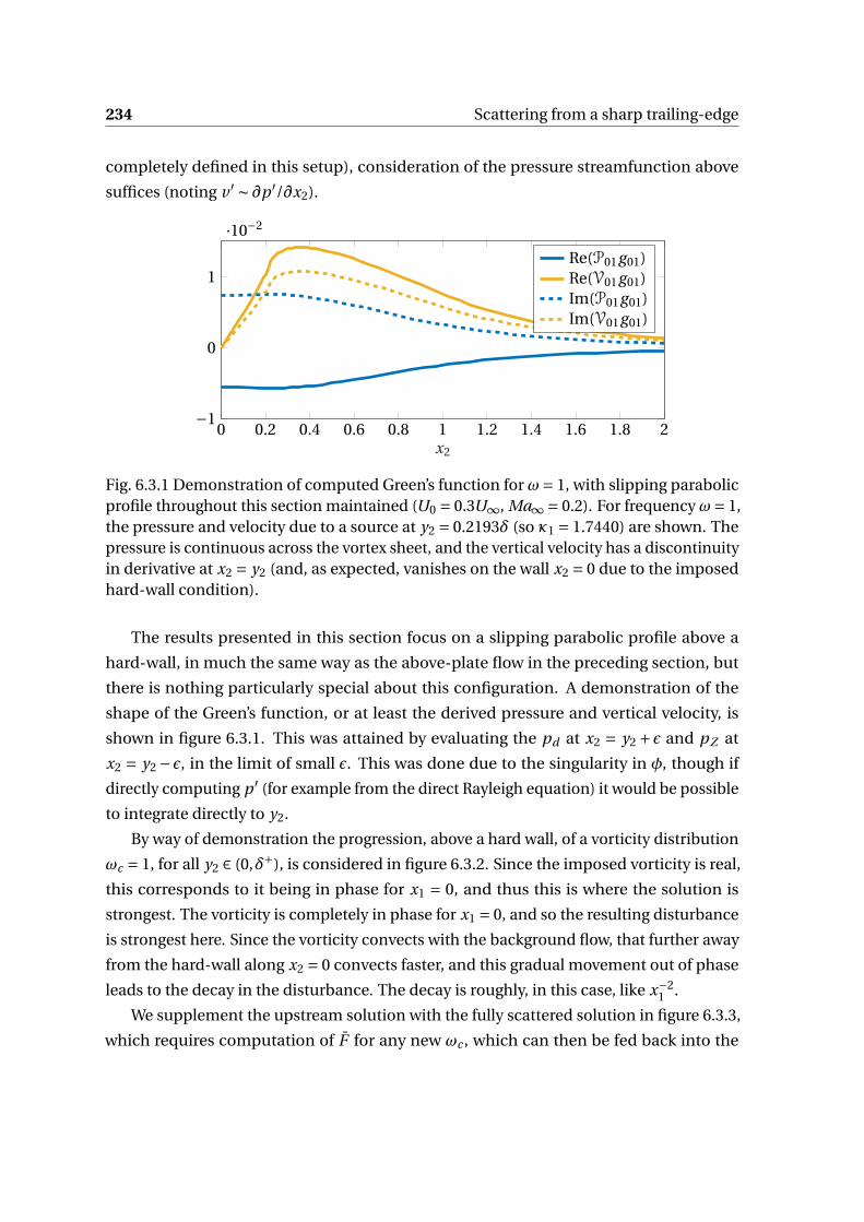
234 Scattering from a sharp trailing-edge

completely defined in this setup), consideration of the pressure streamfunction above

suffices (noting v ′ ∼ ∂p ′/∂x2).

0 0.2 0.4 0.6 0.8 1 1.2 1.4 1.6 1.8 2−1

0

1

·10−2

x2

Re(P01g01)Re(V01g01)Im(P01g01)Im(V01g01)

Fig. 6.3.1 Demonstration of computed Green’s function for ω= 1, with slipping parabolicprofile throughout this section maintained (U0 = 0.3U∞, Ma∞ = 0.2). For frequency ω= 1,the pressure and velocity due to a source at y2 = 0.2193δ (so κ1 = 1.7440) are shown. Thepressure is continuous across the vortex sheet, and the vertical velocity has a discontinuityin derivative at x2 = y2 (and, as expected, vanishes on the wall x2 = 0 due to the imposedhard-wall condition).

The results presented in this section focus on a slipping parabolic profile above a

hard-wall, in much the same way as the above-plate flow in the preceding section, but

there is nothing particularly special about this configuration. A demonstration of the

shape of the Green’s function, or at least the derived pressure and vertical velocity, is

shown in figure 6.3.1. This was attained by evaluating the pd at x2 = y2 + ϵ and pZ at

x2 = y2 − ϵ, in the limit of small ϵ. This was done due to the singularity in φ, though if

directly computing p ′ (for example from the direct Rayleigh equation) it would be possible

to integrate directly to y2.

By way of demonstration the progression, above a hard wall, of a vorticity distribution

ωc = 1, for all y2 ∈ (0,δ+), is considered in figure 6.3.2. Since the imposed vorticity is real,

this corresponds to it being in phase for x1 = 0, and thus this is where the solution is

strongest. The vorticity is completely in phase for x1 = 0, and so the resulting disturbance

is strongest here. Since the vorticity convects with the background flow, that further away

from the hard-wall along x2 = 0 convects faster, and this gradual movement out of phase

leads to the decay in the disturbance. The decay is roughly, in this case, like x−21 .

We supplement the upstream solution with the fully scattered solution in figure 6.3.3,

which requires computation of F for any new ωc , which can then be fed back into the

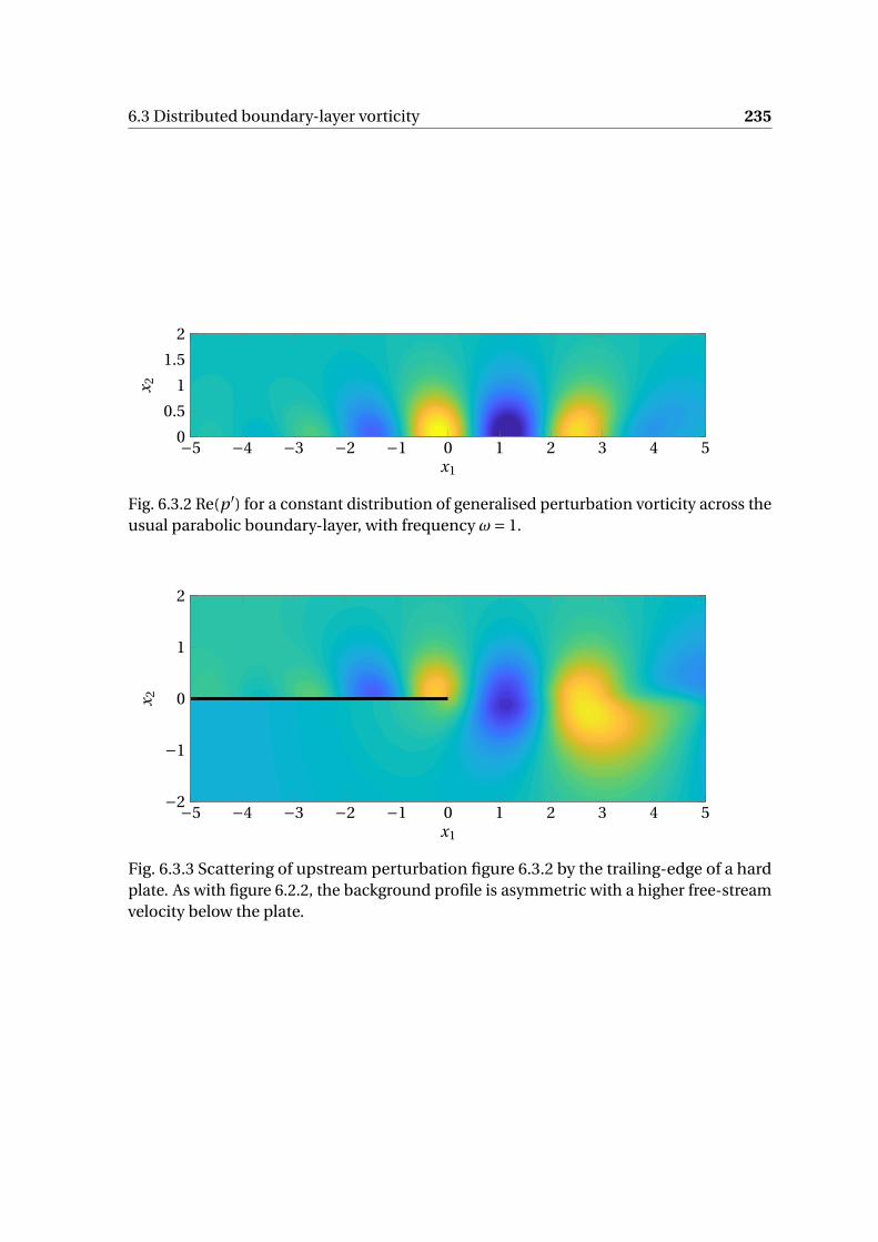
6.3 Distributed boundary-layer vorticity 235

−5 −4 −3 −2 −1 0 1 2 3 4 50

0.5

1

1.5

2

x1

x 2

Fig. 6.3.2 Re(p ′) for a constant distribution of generalised perturbation vorticity across theusual parabolic boundary-layer, with frequency ω= 1.

−5 −4 −3 −2 −1 0 1 2 3 4 5−2

−1

0

1

2

x1

x 2

Fig. 6.3.3 Scattering of upstream perturbation figure 6.3.2 by the trailing-edge of a hardplate. As with figure 6.2.2, the background profile is asymmetric with a higher free-streamvelocity below the plate.

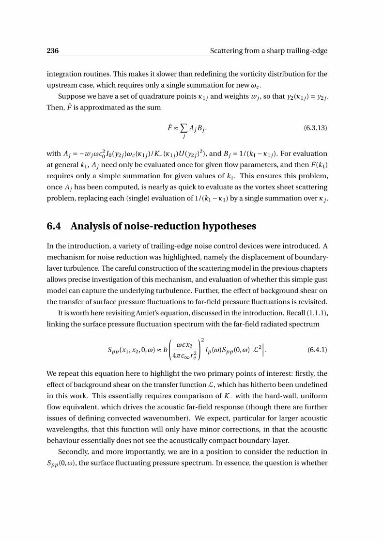
236 Scattering from a sharp trailing-edge

integration routines. This makes it slower than redefining the vorticity distribution for the

upstream case, which requires only a single summation for new ωc .

Suppose we have a set of quadrature points κ1 j and weights w j , so that y2(κ1 j ) = y2 j .

Then, F is approximated as the sum

F ≈∑j

A j B j . (6.3.13)

with A j =−w jωc20 I0(y2 j )ωc (κ1 j )/K−(κ1 j )U (y2 j )2), and B j = 1/(k1 −κ1 j ). For evaluation

at general k1, A j need only be evaluated once for given flow parameters, and then F (k1)

requires only a simple summation for given values of k1. This ensures this problem,

once A j has been computed, is nearly as quick to evaluate as the vortex sheet scattering

problem, replacing each (single) evaluation of 1/(k1 −κ1) by a single summation over κ j .

6.4 Analysis of noise-reduction hypotheses

In the introduction, a variety of trailing-edge noise control devices were introduced. A

mechanism for noise reduction was highlighted, namely the displacement of boundary-

layer turbulence. The careful construction of the scattering model in the previous chapters

allows precise investigation of this mechanism, and evaluation of whether this simple gust

model can capture the underlying turbulence. Further, the effect of background shear on

the transfer of surface pressure fluctuations to far-field pressure fluctuations is revisited.

It is worth here revisiting Amiet’s equation, discussed in the introduction. Recall (1.1.1),

linking the surface pressure fluctuation spectrum with the far-field radiated spectrum

Spp (x1, x2,0,ω) ≈ b

(ωcx2

4πc∞r 2e

)2

lp (ω)Spp (0,ω)∣∣∣L2

∣∣∣ . (6.4.1)

We repeat this equation here to highlight the two primary points of interest: firstly, the

effect of background shear on the transfer function L, which has hitherto been undefined

in this work. This essentially requires comparison of K− with the hard-wall, uniform

flow equivalent, which drives the acoustic far-field response (though there are further

issues of defining convected wavenumber). We expect, particular for larger acoustic

wavelengths, that this function will only have minor corrections, in that the acoustic

behaviour essentially does not see the acoustically compact boundary-layer.

Secondly, and more importantly, we are in a position to consider the reduction in

Spp (0,ω), the surface fluctuating pressure spectrum. In essence, the question is whether

6.4 Analysis of noise-reduction hypotheses 237

we can match displacement of boundary-layer turbulence above noise control devices, an

effect repeatedly borne out in experimental investigations, with a corresponding reduction

in surface pressure fluctuations, using the vortex sheet (and distributed vorticity) models

outlined above, and the resulting wall-pressure due to a known “strength” of vorticity.

6.4.1 Modification of the transfer function by shear layer

In uniform flow, we regain the classical Schwarzschild solution [97, 95] to the trailing-edge

scattering problem, from which Amiet’s transfer function can be constructed. In uniform

flow U , φd = e−γx2 exactly, and the pressure generated from a vortex sheet, via the earlier

calculations, is

P0g (s)0 = I0(y2)γ−(κ1)

2(2πi )

∫F1

e−γ(k1)x2−i k1x1

γ−(k1)(k1 −κ1)dk1

=−e−γ(κ1)y2C (κ1)2

4πiγ+(κ1)c20

∫F1

e−γ(k1)x2−i k1x1

γ−(k1)(k1 −κ1)dk1

(6.4.2)

A gust convecting at the free-stream velocity is silent, since C (ω/U ) = 0 by definition,

and so κ1 must be chosen to correspond to some convected velocity Uc <U , an artificial

constraint bypassed by this more sophisticated calculation. This method is slightly more

general than Schwarszchild’s solution, which merely determines the pressure on the

upstream hard plate, as this incorporates the wall-normal dependence and therefore

allows direct evaluation of far-field sound.

The Wiener-Hopf kernel in the uniform flow case is simply

K = 2Dp

Dh=−2C

γ. (6.4.3)

This is factorised as K+ = 2γ+/C and K− = 1/γ−(k1), and the former appears outside the

integrand, evaluated at convected wavenumber κ1, and the latter within the integrand.

The effect of shear can then be quantified in the effect on the behaviour of K+(κ1)K−(k1).

An ideal consideration would be investigation of the behaviour of source-independent

functions γ−(k1) and K−(k1), but this runs into issues with the ability to arbitrarily scale

the factorised kernel by an arbitrary constant. This, essentially, is the same as the previous

computation of far-field noise, but we are interested here only in the transmission of

wall-pressure fluctuations to far-field pressure fluctuations, which arises from fixing I0 ≡ 1,

considering the scattering of the gust-induced wall-pressure e i (ωt−iκ1x1), where we now

238 Scattering from a sharp trailing-edge

must prescribe κ1. Fixing Uc = 0.8U0 for all plots1, the far-field sound in two cases for unit

I0, as the boundary-layer profile is consistently varied, is shown in figure 6.4.1.

We consider the two distinct cases of an acoustically compact boundary-layer, and

one which is less so. In both cases, we consider a slipping parabolic profile though there

is no reason the results will not be generic. Identification of the source strength (here,

I0 = 1) allows far-field directivity to be exactly plotted including magnitude, and both plots

show the magnitude of far-field pressure |p ′|, up to the decay as r−1/2. In the first case, the

acoustic wavelength λa = 20πδ, much larger than the boundary-layer thickness, whereas

in the second case λa = 2πδ, which is a comparable size to the boundary-layer thickness.

As previously identified, the directivity of the scattering is essentially unmodified by the

compact boundary-layer, though there is variation for shorter acoustic wavelengths. In

both cases, we compare with the cardioid profile obtained for uniform flow (U0 =U∞),

slightly shifted from a sin(θ/2) profile by Mach number effects.

Allowing for observation of the magnitude variation allows identification of a small

enhancement in sound by boundary-layer shear, with the lowest slip velocity, in both

cases, leading to the highest radiation. The effect is noticeably reduced in the compact

case, and is only maximally up to 2 dB in the shorter wavelength case. As hypothesised,

there is little effect on radiation directly from the boundary-layer shear, particularly in

the longer wavelength cases of interest (driven by low free-stream Mach number, rather

than low frequency). This highlights the need to directly consider the effect of source

on reducing wall-pressure fluctuations (and therefore, by this analysis, far-field pressure

fluctuations).

6.4.2 Reduction of wall pressure by vorticity displacement

Having identified F with generalised convected vorticity ωc , we can turn attention to

a fundamental question of this thesis, namely the potential reduction of far-field noise

through the displacement of boundary-layer turbulence. For an infinitesimal vortex

sheet at location x2 = y2, of strength ω0, we have an explicit expression for the induced

wall-pressure pw given by

pw =−ω0c0(y2)2I0

U ′(y2)= ω0

C (0;κ1)U ′(y2)

pd (y2;κ1)ℓZ1 (κ1)

D1Z (κ1(y2))

. (6.4.4)

1This value of Uc is somewhat arbitrary, and is merely used as an example. Measured convection velocitiesare a function of frequency, with Rogers and Moreau [94] encorporating Uc = 0.6U∞ in their extension ofAmiet’s models, and Uc = 0.7U∞ often used.

6.4 Analysis of noise-reduction hypotheses 239

0

π/6

π/3θ =π/2

π

5π/6

2π/3

−π/6

−π/3−π/2

−5π/6

−2π/3

r = 0.5r = 1

r = 1.5

U0 = 0.2U∞U0 = 0.6U∞U0 =U∞

(a) Acoustically compact boundary-layer, c0 = 50U∞.

0

π/6

π/3θ =π/2

π

5π/6

2π/3

−π/6

−π/3−π/2

−5π/6

−2π/3

r = 0.2r = 0.4

U0 = 0.2U∞U0 = 0.6U∞U0 =U∞

(b) Acoustically non-compact boundary-layer, c0 = 5U∞.

Fig. 6.4.1 The transfer of wall-pressure to the far-field for a parabolic slipping profile, atfrequency ω= 5, with gust wavenumber κ1 =ω/(0.8U∞).

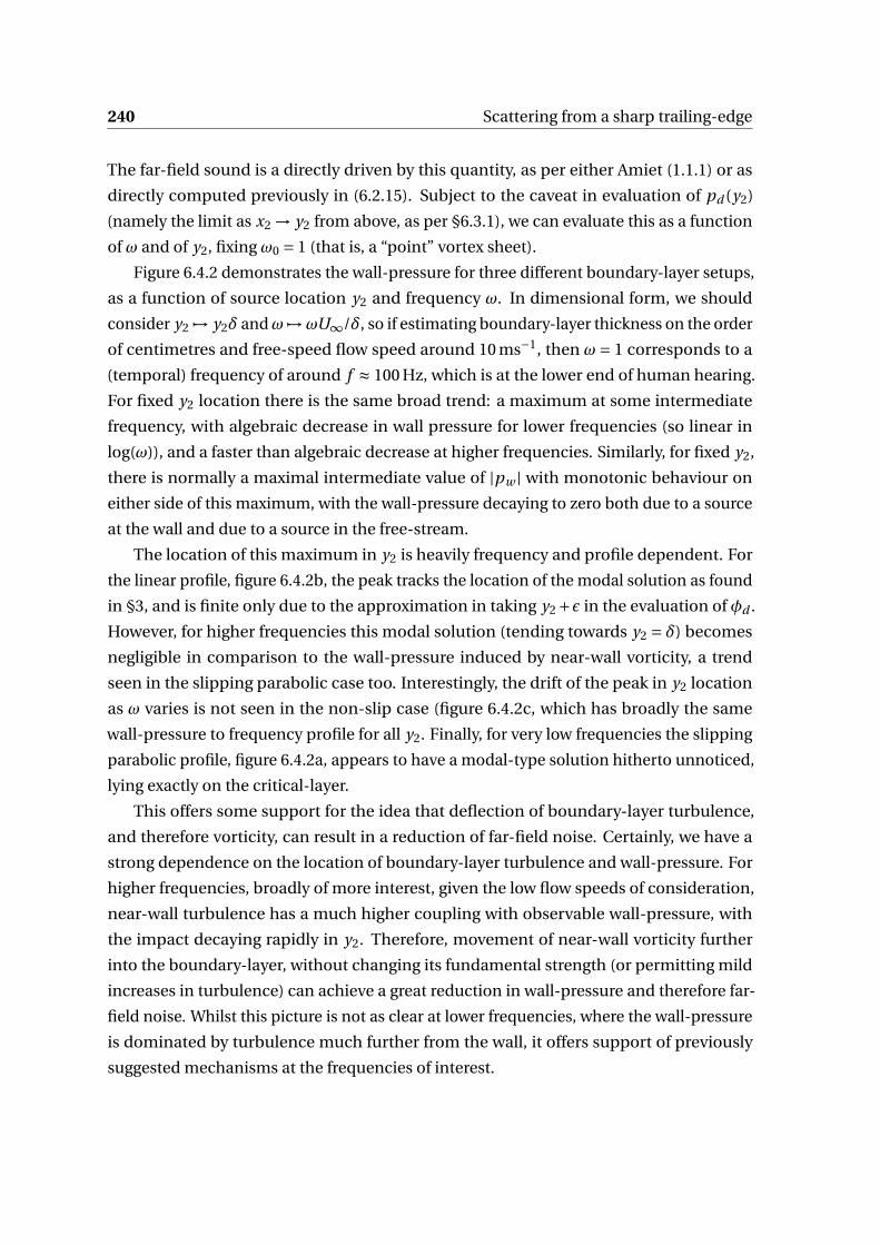
240 Scattering from a sharp trailing-edge

The far-field sound is a directly driven by this quantity, as per either Amiet (1.1.1) or as

directly computed previously in (6.2.15). Subject to the caveat in evaluation of pd (y2)

(namely the limit as x2 → y2 from above, as per §6.3.1), we can evaluate this as a function

of ω and of y2, fixing ω0 = 1 (that is, a “point” vortex sheet).

Figure 6.4.2 demonstrates the wall-pressure for three different boundary-layer setups,

as a function of source location y2 and frequency ω. In dimensional form, we should

consider y2 7→ y2δ andω 7→ωU∞/δ, so if estimating boundary-layer thickness on the order

of centimetres and free-speed flow speed around 10 ms−1, then ω= 1 corresponds to a

(temporal) frequency of around f ≈ 100 Hz, which is at the lower end of human hearing.

For fixed y2 location there is the same broad trend: a maximum at some intermediate

frequency, with algebraic decrease in wall pressure for lower frequencies (so linear in

log(ω)), and a faster than algebraic decrease at higher frequencies. Similarly, for fixed y2,

there is normally a maximal intermediate value of |pw | with monotonic behaviour on

either side of this maximum, with the wall-pressure decaying to zero both due to a source

at the wall and due to a source in the free-stream.

The location of this maximum in y2 is heavily frequency and profile dependent. For

the linear profile, figure 6.4.2b, the peak tracks the location of the modal solution as found

in §3, and is finite only due to the approximation in taking y2 +ϵ in the evaluation of φd .

However, for higher frequencies this modal solution (tending towards y2 = δ) becomes

negligible in comparison to the wall-pressure induced by near-wall vorticity, a trend

seen in the slipping parabolic case too. Interestingly, the drift of the peak in y2 location

as ω varies is not seen in the non-slip case (figure 6.4.2c, which has broadly the same

wall-pressure to frequency profile for all y2. Finally, for very low frequencies the slipping

parabolic profile, figure 6.4.2a, appears to have a modal-type solution hitherto unnoticed,

lying exactly on the critical-layer.

This offers some support for the idea that deflection of boundary-layer turbulence,

and therefore vorticity, can result in a reduction of far-field noise. Certainly, we have a

strong dependence on the location of boundary-layer turbulence and wall-pressure. For

higher frequencies, broadly of more interest, given the low flow speeds of consideration,

near-wall turbulence has a much higher coupling with observable wall-pressure, with

the impact decaying rapidly in y2. Therefore, movement of near-wall vorticity further

into the boundary-layer, without changing its fundamental strength (or permitting mild

increases in turbulence) can achieve a great reduction in wall-pressure and therefore far-

field noise. Whilst this picture is not as clear at lower frequencies, where the wall-pressure

is dominated by turbulence much further from the wall, it offers support of previously

suggested mechanisms at the frequencies of interest.

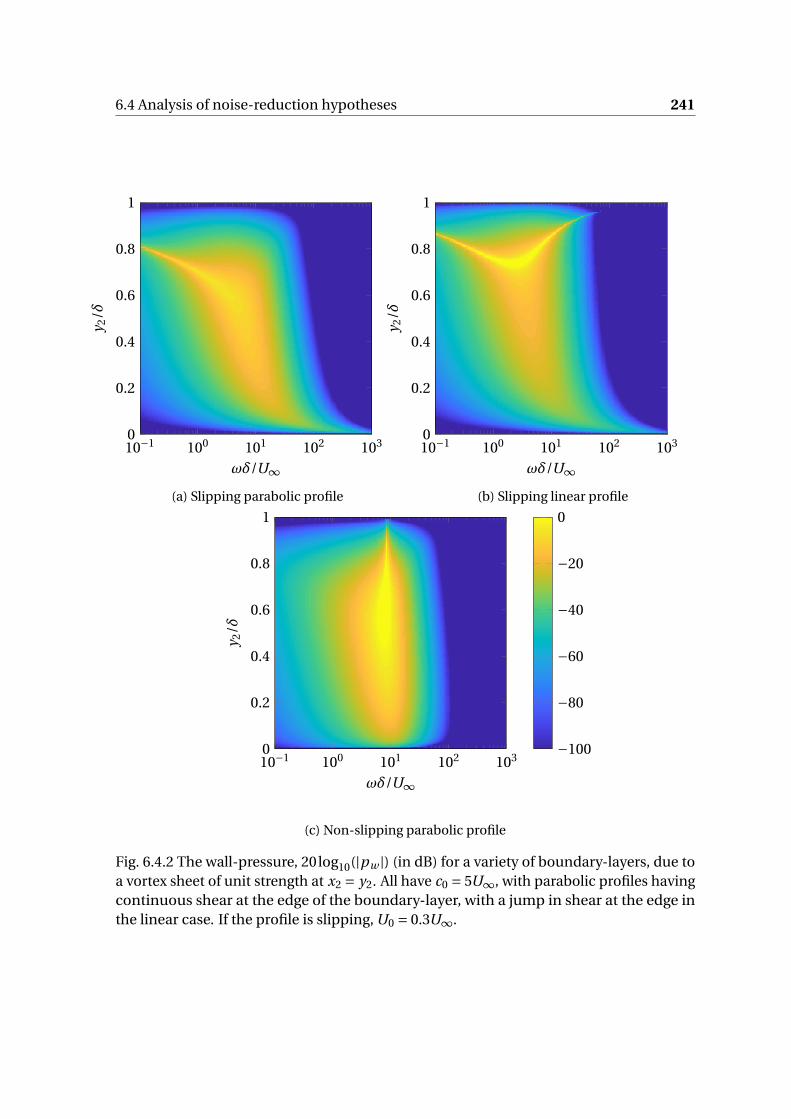
6.4 Analysis of noise-reduction hypotheses 241

10−1 100 101 102 1030

0.2

0.4

0.6

0.8

1

ωδ/U∞

y 2/δ

(a) Slipping parabolic profile

10−1 100 101 102 1030

0.2

0.4

0.6

0.8

1

ωδ/U∞

y 2/δ

(b) Slipping linear profile

10−1 100 101 102 1030

0.2

0.4

0.6

0.8

1

ωδ/U∞

y 2/δ

−100

−80

−60

−40

−20

0

(c) Non-slipping parabolic profile

Fig. 6.4.2 The wall-pressure, 20log10(|pw |) (in dB) for a variety of boundary-layers, due toa vortex sheet of unit strength at x2 = y2. All have c0 = 5U∞, with parabolic profiles havingcontinuous shear at the edge of the boundary-layer, with a jump in shear at the edge inthe linear case. If the profile is slipping, U0 = 0.3U∞.

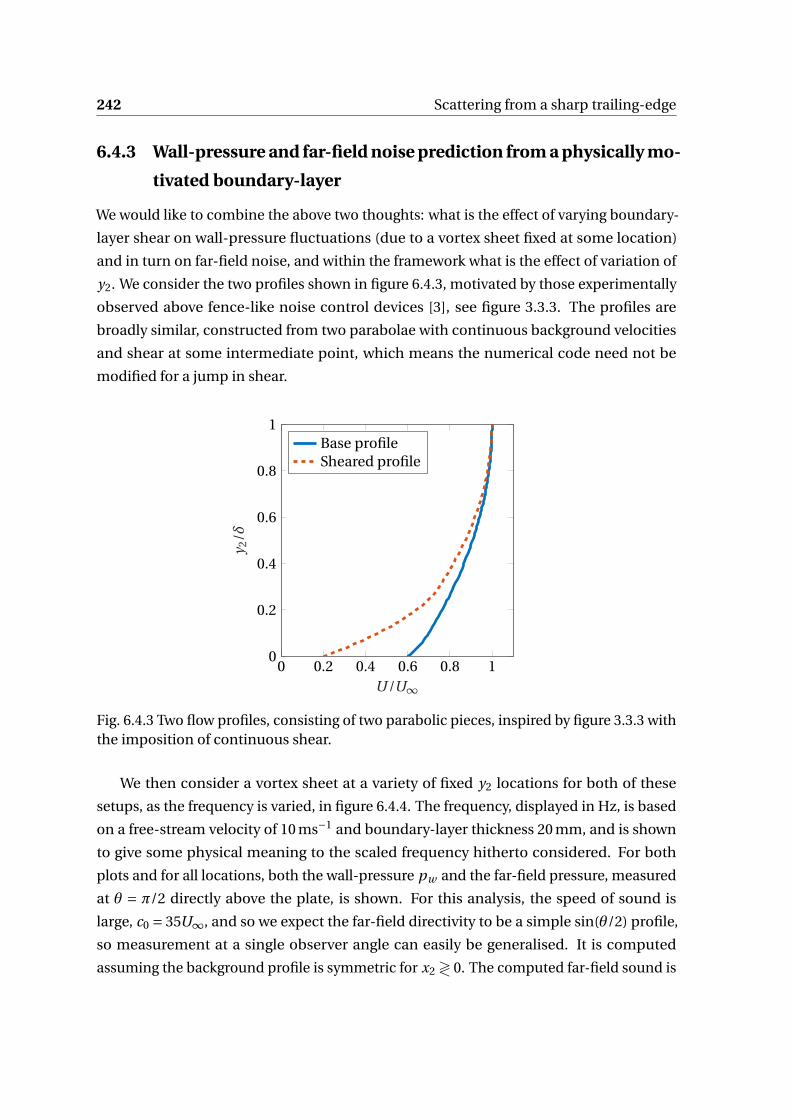
242 Scattering from a sharp trailing-edge

6.4.3 Wall-pressure and far-field noise prediction from a physically mo-

tivated boundary-layer

We would like to combine the above two thoughts: what is the effect of varying boundary-

layer shear on wall-pressure fluctuations (due to a vortex sheet fixed at some location)

and in turn on far-field noise, and within the framework what is the effect of variation of

y2. We consider the two profiles shown in figure 6.4.3, motivated by those experimentally

observed above fence-like noise control devices [3], see figure 3.3.3. The profiles are

broadly similar, constructed from two parabolae with continuous background velocities

and shear at some intermediate point, which means the numerical code need not be

modified for a jump in shear.

0 0.2 0.4 0.6 0.8 10

0.2

0.4

0.6

0.8

1

U /U∞

y 2/δ

Base profileSheared profile

Fig. 6.4.3 Two flow profiles, consisting of two parabolic pieces, inspired by figure 3.3.3 withthe imposition of continuous shear.

We then consider a vortex sheet at a variety of fixed y2 locations for both of these

setups, as the frequency is varied, in figure 6.4.4. The frequency, displayed in Hz, is based

on a free-stream velocity of 10 ms−1 and boundary-layer thickness 20 mm, and is shown

to give some physical meaning to the scaled frequency hitherto considered. For both

plots and for all locations, both the wall-pressure pw and the far-field pressure, measured

at θ = π/2 directly above the plate, is shown. For this analysis, the speed of sound is

large, c0 = 35U∞, and so we expect the far-field directivity to be a simple sin(θ/2) profile,

so measurement at a single observer angle can easily be generalised. It is computed

assuming the background profile is symmetric for x2 ≷ 0. The computed far-field sound is

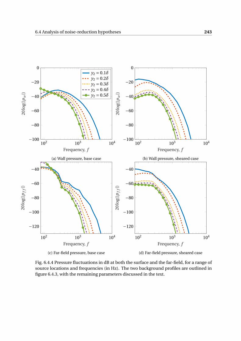
6.4 Analysis of noise-reduction hypotheses 243

102 103 104−100

−80

−60

−40

−20

0

Frequency, f

20lo

g(|p

w|)

y2 = 0.1δy2 = 0.2δy2 = 0.3δy2 = 0.4δy2 = 0.5δ

(a) Wall pressure, base case

102 103 104−100

−80

−60

−40

−20

0

Frequency, f

20lo

g(|p

w|)

(b) Wall pressure, sheared case

102 103 104

−120

−100

−80

−60

−40

Frequency, f

20lo

g(|p

ff|)

(c) Far-field pressure, base case

102 103 104

−120

−100

−80

−60

−40

Frequency, f

20lo

g(|p

ff|)

(d) Far-field pressure, sheared case

Fig. 6.4.4 Pressure fluctuations in dB at both the surface and the far-field, for a range ofsource locations and frequencies (in Hz). The two background profiles are outlined infigure 6.4.3, with the remaining parameters discussed in the text.

244 Scattering from a sharp trailing-edge

102 103 104

−40

−20

0

20

40

Frequency, f

20lo

g(|p

wsh

eare

d/p

wb

ase|)

y2 = 0.1δy2 = 0.2δy2 = 0.3δy2 = 0.4δy2 = 0.5δ

(a) Reduction of wall-pressure fluctuationsthrough introduction of shear profile

102 103 104

−40

−20

0

20

40

Frequency, f

20lo

g(|p

ffs

hea

red

/pf

fbas

e|)

(b) Reduction in far-field noise through in-troduction of sheared profile

Fig. 6.4.5 Change in pressure fluctuations (in dB) due to the change in background profile,as figures 6.4.3 and 6.4.4.

the magnitude of a wave decaying as r−1/2, and this factor (and other scaling constants,

irrelevant on a logarithmic scale) have been ignored. The far-field noise is derived as a

multiplier of the wall-pressure, which does depend to a limited extent on frequency and

source location (as well as boundary-layer shape).

There are features common to all the plots. As before, for fixed y2 there is a maximal

value of wall-pressure at some intermediate frequency (both figures 6.4.4a and 6.4.4b),

though this property doesn’t neatly transfer to far-field noise. The magnitude of this peak

is monotonic in y2, with the wall-pressure decreasing as y2 increases. Indeed, this is

common to almost all frequencies of interest: a vortex sheet further from the wall, with

the same magnitude of vorticity, induces a smaller wall-pressure. This monotonicity is

preserved in the far-field, figures 6.4.4c and 6.4.4d. At low frequencies, the increase in

wall-presure with frequency does not transfer to an increase in far-field pressure with

frequency.

At physically realisable frequencies, the common decrease in wall-pressure with in-

crease in y2 lends a great deal of support to the hypothesis that turbulence deflection

leads to a reduction in wall-pressure and, through this scattering model, far-field noise.

The reduction is not insubstantial, particularly at higher frequencies, though it is worth

noting it is at these frequencies we might expect the viscous terms, hitherto neglected, to

become important.

6.5 Conclusions and discussion 245

We can use the choice of two background profiles to investigate the effect of back-

ground shear on both wall-pressure and radiated noise directly, as per figure 6.4.5, which

looks at the decibel increase in both wall-pressure and far-field noise in the sheared

case, compared with the base case. This highlights an important warning about use of

wall-pressure as a proxy for far-field noise: whilst there is broadly, for all frequencies,

a reduction in far-field noise (with some small increase at some y2 when log( f ) ≈ 2.5),

there appears to be an increase in wall-pressure at low frequencies when the source is

near the wall, amplified by the increase in shear. This is consistent with the work in §3.5,

which looked at the effect of a (piecewise linear) background profile with increased shear

near the wall, and showed an increase in wall-pressure. That this need not translate into

increased far-field noise adds substance to the effect of shear-shielding, even if there is

some apparent increase in wall-pressure. An increase in wall-pressure directly due to the

background profile could be directly cancelled out in the scattering to the far-field.

With this we have established that both a change in background profile, and a move-

ment of vorticity within the boundary-layer, can lead to a substantial reduction in observed

far-field noise. The movement of vorticity consistently and predictably leads to a reduc-

tion in far-field noise, where the change of the background profile is less clear-cut, which

supports the work presented in the previous two sections.

6.5 Conclusions and discussion

By extension of the Wiener-Hopf process introduced in §5, this chapter outlines the

solution to the generic scattering problem from a trailing-edge. Typical analyses of this

kind of problem assume the underlying differential equation, under a suitable integral

transformation (be it Fourier or equivalently Laplace, as in this work, or for example the

Mellin transform when considering wedge scattering), can be reduced to an ODE for

which analytic solutions can be obtained. The numerical work then arises from the need

to factorise the Wiener-Hopf kernel, but with a complete understanding of the complex

analytic behaviour of this kernel. The work in §5 and this chapter has generally kept the

factorisation and therefore the solution of the problem quite simple, by only considering a

single junction (or, in the trailing-edge case, two junctions linked by the behaviour of the

solution across the wake). However, complexity has arisen as the governing transformed

ODE does not permit simple, analytic, closed form solutions, and therefore numerical

routines have been introduced to allow the Wiener-Hopf framework to be used, which

was the fundamental basis for the work of §4.

246 Scattering from a sharp trailing-edge

Through the framework developed throughout this work, it is numerically inexpensive

to quickly determine the far-field noise due to scattering of a vortex sheet, and indeed a

more generic “gust” solution, from a sharp trailing-edge. This extends the typical work

concerning uniform flow, or symmetric flow with constant shear [96], to more general

background profiles, which may be both asymmetric and have smoothly varying shear.

Further, this work has extended typical considerations of scattering from a hard- or a

pressure-release wall to scattering from a generic lined wall, subject to the caveat that

the impedance Z is equal on both surfaces of the plate, permitting solution (as a scalar

Wiener-Hopf problem) through proportionality of pressure and velocity perturbations

along x2 = 0. The more generic case, with different impedances above and below the plate,

requires use of more sophisticated matrix-based Wiener-Hopf techniques, and is unlikely

to result in solutions that can easily be written down in closed form.

A primary outcome of this chapter is the construction of a more generic gust solution,

given some known vorticity distribution at some physical location, following Goldstein’s

work [46, 48]. Identifying the convected quantity with some generalised perturbation

vorticity allows analysis of the effect of displacement of this vorticity within the boundary-

layer. In the final section, §6.4, this was used to consider the questions outlined in

the introduction to this thesis: namely can these reasonably simple models give some

understanding of the workings of noise control devices, which appear to work via the

deflection of boundary-layer turbulence away from the scattering wall, resulting in a

reduction in surface pressure and in turn a reduction in far-field noise. Whilst direct

modification of boundary-layer mean shear does little to the far-field radiation, in fact

broadly increasing it, there is strong evidence that vorticity movement with the boundary-

layer (and therefore movement of turbulence) has a strong effect on reduction of surface

pressure. In particular, at high frequencies surface pressure is dominated by vorticity very

near the scattering surface, so displacement of these disturbances, even if the effect is

only small, can have a large effect on far-field noise.

Chapter 7

Conclusions

7.1 Summary and discussion

7.1.1 Implementation of quasi-numerical methods

This work fits between the two typical approaches to scattering problems.

The first, broadly analytic, relies on the the governing ODE having analytic solutions

so the Wiener-Hopf process can be done almost entirely in terms of known functions.

Any numerical computations in this procedure are normally focused on the factorisation

of the Wiener-Hopf kernel. Alternatively, when there is more than one junction and the

perturbations are governed by a matrix Wiener-Hopf equation (for example scattering by

a thin plate of finite length), iterative methods can be used to compute the solution via a

series of scalar Wiener-Hopf problems. Other problems consider a background flow that

is some small irrotational perturbations to some uniform flow, for example the noise of a

cambered, angled or thick aerofoil [75, 76, 9]. However, in the limit chosen for acoustic

perturbations, these perturbations are generally governed by Helmholtz equation, or can

at least be reduced to this form, or alternative asymptotic limits can be considered which

give rise to analytic solutions (for example with background shear [10]). Only rarely has

the case where the governing ODE itself cannot be solved analytically been considered.

Whilst this work began with a case for which analytically tractable solutions could be

found (§3), it was identified that as the number of piecewise linear pieces was increased

this process was no longer practical. Similarly, in the compressible case, with a linearly

sheared boundary-layer of finite extent, it is possible to find a solution to the govern-

ing ODE for pressure in terms of hypergeometric functions [96]. These are of no help

when considering the scattering problem, as they are less well-understood functions that,

broadly, can only be considered numerically. The Wiener-Hopf process, however, requires

248 Conclusions

only a limited amount of knowledge about the functions being considered: the far-field

behaviour of the Wiener-Hopf kernel, whether or not this kernel has zeros and poles, and

which generalised half-plane it lies in, as well as some knowledge of branch points. All of

these can be gleaned from a function defined only as a solution to an ODE with specified

boundary conditions, and it is this approach taken throughout this work.

For the problem considered, the branch cuts are imposed by the behaviour at the edge

of the boundary-layer, and are therefore well-understood. The work of chapters 3 and 4

primarily considered the mass source problem, but also allowed consideration of roots

of a variety of dispersion relations, which (as demonstrated in §5.2) have a direct link to

zeros and poles of the Wiener-Hopf kernel. With this, the complete information required

to solve the Wiener-Hopf kernel has been obtained without explicit analytic solution of

the governing ODE. This comes at the cost of increased computational expense, though

computation of the auxiliary functions for a governing ODE is comparatively inexpensive

when compared with the kernel factorisation process (which does however have auxiliary

function computation embedded within it).

The second approach is complete numerical computation of the scattered solution.

Grid based methods struggle with scattering problems due to the large number of points

required near the boundary-layer discontinuity. Indeed, for genuinely discontinuous

boundary-conditions, the difficulty of eliminating eigenfunctions of the scattered solu-

tion, through an imposition of a Kutta condition, becomes difficult [8]. Aside from the

comparatively inexpensive routines developed in this work, the satisfaction of the Kutta

condition trivially requires specification of a single entire function E , which can be eval-

uated on physical grounds. Finally, this setup naturally leads to propagating wavelike

solutions in an infinite domain, avoiding problems of reflection from the edge of the

domain typically found in numerical applications.

Finding the middle ground between these approaches, as we have done in this thesis,

vastly increases the number of problems for which the Wiener-Hopf technique can be

used, across a wider range of the parameter space (in particular at all but the very high

frequencies at which viscous effects become important).

7.1.2 Development of the understanding of scattering problems

The solution of scattering problems induced by a discontinuity in boundary conditions is

not new, and neither is the use of the Wiener-Hopf technique in solving them. However,

the inclusion of background shear within the scattering problem reduces many analytic

complexities of the hard-soft scattering problem, at the expense of the a more complex

governing ODE that does not necessarily permit analytical solutions, discussed above.

7.1 Summary and discussion 249

As noted in the introduction to §5, the scattering from lined surfaces has previously

thrown up difficulties. Consideration of the hard-soft scattering problem, with mean flow,

is not new [89, 93], though due to the presence of surface modes a variety of modelling

simplifications have previously been made, for example assuming a thin region near the

wall in which there is no background flow, or by considering an unbounded region of

constant shear. These modelling simplifications are needed due to the presence of surface

modes, which may be convectively unstable, and exist only in an exponentially thin region

near the wall (when considering perturbations to uniform flow). Modifications to the

Myers boundary condition have been proposed to deal with this difficulty [66], though

little work has been done on the scattering problem with these new boundary conditions.

By allowing a non-infinitesimal boundary-layer, we have revisited the scattering prob-

lem, deriving a solution which, although it must be computed numerically, satisfies the

boundary conditions and, more importantly, any conditions imposed at the scattering

junction. That this solution is correct can readily be shown by verifying the computed so-

lutions, though a considerable deal of work has been put into the generation of near-field

solutions demonstrating the behaviour of the perturbation within the boundary-layer.

An important result is the clarification that, in the limit of c0 → ∞, the scattered

solution across a hard-soft junction regains the cardioid-type scattering that would be

expected of scattering from a hard trailing-edge, and indeed later we see the the soft-hard

scattering directivity is directly comparable to the scattering from a soft trailing-edge. This

limit, the limit of long acoustic wavelength and the quasi-incompressible limit, has been

analysed previously analytically [93, 101], though direct analysis of this setup is difficult.

By direct numerical consideration of the limit, exact results have been generated.

Finally, it is worth reviewing the problem considered in §5.6, in which a convectively

unstable surface mode (be it above an lined surface or a pressure-release wall) may

restabilise at the trailing-edge of the lined section, as the hard-wall downstream cannot

support such disturbances. It was demonstrated that such modes can lead to a large

increase in scattered acoustic noise due to a finite section of lining, due to the exponential

growth of the surface mode even over the comparatively short distances involved. Whilst

this surface mode is in some sense invisible (since it doesn’t propagate downstream), its

large contribution to the acoustic scattering suggests a need for care, and highlights the

importance in understanding these modes.

7.1.3 Explaining noise control devices

This work began with a discussion of novel devices for the control of trailing-edge noise.

There was particular focus on two broad types of devices: firstly, blowing near the trailing-

250 Conclusions

edge [106], and secondly through streamwise-orientated devices structures upstream

of the trailing-edge, be it fibres [28, 27], rails [25], or fence-like finlets [26, 24, 3, 4]. All

these devices (both passive and active) reduce the pressure fluctuations on the scattering

surface of the aerofoil, and thus (either directly measured or inferred via some modelled

transfer function) result in a (sometimes substantial) reduction of far-field noise, with

obvious practical applications including the blades of wind turbines. The passive devices

took inspiration from the soft, downy coating on the upper side of an owl’s wing, which

has the effect of almost completely suppressing pressure fluctuations, and contributes

substantially to the silent flight of larger owl species.

Experimental measurements of both blowing and streamwise-aligned passive devices

results in two observations, common to both devices. As the flow passes over the device,

there is a sharp increase in near wall mean shear. As the flow develops, there is a region of

recirculation in the wake of the device. Flow-borne turbulence from upstream is therefore

deflected further away from the wall, above this recirculation region, a result apparent in

measurements of rms velocity perturbations within the boundary-layer. Some experimen-

tal setups allow measurement of both background shear and of turbulence intensity at a

variety of streamwise locations, from which a reasonably complete understanding of the

flow over such devices can be obtained [106].

A goal of this work was to construct an analytical framework that could utilise these

experimental observations directly, importantly isolating the acoustically relevant mech-

anisms. This model was created through Goldstein’s work on Rapid Distortion Theory

[43, 44], which directly includes the effects of mean flow shear and provides a careful

framework for gust solutions, namely generalised vortical solutions convected with the

mean flow, which are the only contribution to the acoustic (pressure) components of

the far-field disturbance. To some extent, all chapters of this thesis relate to applying

this theory in a more and more complicated framework, in particular to the problem of

scattering from a trailing-edge. With the mean flow profile and perturbation vorticity (as a

proxy for turbulence intensity) now as inputs to the model, it has been demonstrated that

it is possible to compute both the near- and far-field scattering of an arbitrary vorticity

distribution to an arbitrary (continuous) mean flow.

This allows testing of both the experimental observations, which was done in §6.4,

asking two questions. Firstly, how does mean background shear affect the transfer of wall-

pressure fluctuations to far-field pressure fluctuations, and secondly can the reduction in

wall-pressure fluctuations be explained by this simple model of boundary-layer turbulence

(ignoring the effects of viscosity and nonlinearity in the mean flow, for example).

7.2 Future work 251

For longer acoustic wavelengths, corresponding to lower frequencies, there is little

difference in radiation to the far-field, which would be predicted by scaling arguments.

Indeed, there is evidence that mean shear enhances far-field noise due to wall-pressure

fluctuations, though compared to observed noise reduction the effect is minimal. There

is, however, a strong relationship between vorticity location within the boundary-layer

and induced wall pressure, dramatically shown in figure 6.4.2. In particular, for higher

frequencies (more comparable to frequencies of interest), disturbances close to the wall

induce a considerably stronger wall-pressure. That this effect is highly dependent on back-

ground shear was investigated more thoroughly in the following section. This confirmed

that displacement of boundary-layer turbulence can indeed result in a large reduction of

wall-pressure, and therefore far-field noise, even for small displacements, provided any

disturbance is moved out of this thin, “loud” region.

Whilst conclusions are as yet limited, this comparatively simple model, focusing on

the underlying physics of noise induced by unsteady fluctuations within the boundary-

layer, has successfully given rise to the required framework to which the experimental

observations on noise control devices can be compared.

7.2 Future work

This work has primarily focused on the construction of a model of gust-junction inter-

action, rather than complete exploration of the possibilities offered by it. The model,

as described mathematically and as numerically implemented, permits the background

density to vary with the transverse coordinate x2 (via the background speed of sound as

a proxy), a condition that has not been utilised in this work but is appropriate at higher

Mach numbers. Further, this work focused on the purely two-dimensional case, with U

regarded as a function of wall-normal coordinate x2 only. As noted in the introduction,

the formulation permits spanwise dependence of U (and c0), with the derivation relying

only on the parallel nature of the background flow. Three-dimensionality is permitted

in the perturbation via the spanwise wavenumber k3, and the code constructed for this

work permits this to be non-zero though, again, this has not been directly studied in this

work. Further work should consider non-zero k3, particularly as integration over spanwise

lengthscales is important for the complete understanding of far-field noise.

In this work, only finite boundary-layers, with non-zero shear confined to some in-

terval x2 ∈ (δ−,δ+), were considered. There is no fundamental need for this restriction.

The derivation makes no assumption of it, save in the prescription that, in the mean

flow, φd = exp(−γ∞x2). Replacing this with (integrated) φd satisfying φd ∼ exp(−γ∞x2)

252 Conclusions

as x2 →∞, on the assumption that U →U∞ in this limit, permits non-finite boundary-

layers. The boundary-layer integration can be computed by making some mapping of

the infinite integral x2 ∈ (0,∞) to a finite integral, exactly as done with numerical inver-

sion routines. In particular, this would allow consideration of tanh-like profiles and a

Blasius-type boundary-layer profile, which in turn must be computed as the solution to

the governing nonlinear ODE. At reasonably low Reynolds numbers, the Blasius boundary-

layer is physically relevant, and therefore extension of this work to infinite boundary-layers

is very desirable.

The indicative results on gust displacement are interesting, if currently only reasonably

qualitative. This is not a limitation of the model as coded, as it happily permits scattering

of arbitrary vorticity distributions from a trailing-edge or a junction, and further work

should be done to quantify the link between vorticity location and scattered noise, par-

ticularly through utilisation of realistic experimental data, and at physically realisable

frequencies. An important question is, however, raised: what is the link between (measur-

able) boundary-layer velocity fluctuations and boundary-layer vorticity (which drives the

scattering process)? For a practical model that takes, as an input, background shear and

boundary-layer turbulence, this link is a crucial step.

References

[1] Ablowitz, M. J. and Fokas, A. S. (2003). Complex Variables: Introduction and Applica-

tions, volume XXXIII. Cambridge University Press.

[2] Abramowitz, M. and Stegun, I. A. (1965). Handbook of mathematical functions, with

formulas, graphs, and mathematical tables,. Dover Publications, New York.

[3] Afshari, A., Azarpeyvand, M., Dehghan, A. A., and Szoke, M. (2016). Trailing Edge

Noise Reduction Using Novel Surface Treatments. In 22nd AIAA/CEAS Aeroacoustics

Conference, page 2834. AIAA.

[4] Afshari, A., Azarpeyvand, M., Dehghan, A. A., and Szoke, M. (2017). Effects of Stream-

wise Surface Treatments on Trailing Edge Noise Reduction. 23rd AIAA/CEAS Aeroacous-

tics Conference.

[5] Amiet, R. K. (1976). Noise due to turbulent flow past a trailing edge. Journal of Sound

and Vibration, 47(3):387–393.

[6] Amiet, R. K. (1978). Effect of the incident surface pressure field on noise due to

turbulent flow past a trailing edge.

[7] Ayton, L. J. (2017). An analytic solution for gust-aerofoil interaction noise for plates

with leading-edge serrations. In 23rd AIAA/CEAS Aeroacoustics Conference.

[8] Ayton, L. J., Gill, J. R., and Peake, N. (2016). The importance of the unsteady Kutta

condition when modelling gust-aerofoil interaction. Journal of Sound and Vibration,

378:28–37.

[9] Ayton, L. J. and Peake, N. (2013). On high-frequency noise scattering by aerofoils in

flow. Journal of Fluid Mechanics, 734:144–182.

[10] Ayton, L. J. and Peake, N. (2015). On high-frequency sound generated by gust-aerofoil

interaction in shear flow. Journal of Fluid Mechanics, 766:297–325.

254 References

[11] Baker, D. I. and Peake, N. (2018). Trailing-edge noise in slowly-varying, sheared flow.

In 2018 AIAA/CEAS Aeroacoustics Conference, Reston, Virginia. American Institute of

Aeronautics and Astronautics.

[12] Batchelor, G. K. (2000). An Introduction to Fluid Dynamics. Cambridge University

Press.

[13] Batchelor, G. K. and Proudman, I. (1954). The effect of rapid distortion of a fluid in

turbulent motion. Quarterly Journal of Mechanics and Applied Mathematics, 7(1):83–

103.

[14] Bender, C. M. and Orszag, S. A. (2013). Advanced mathematical methods for scientists

and engineers I: Asymptotic methods and perturbation theory. Springer Science &

Business Media.

[15] Bodling, A., Agrawal, B. R., Sharma, A., Clark, I., Alexander, W. N., and Devenport,

W. J. (2017). Numerical Investigation of Bio-Inspired Blade Designs at High Reynolds

Numbers for Ultra-Quiet Aircraft and Wind Turbines. In 23rd AIAA/CEAS Aeroacoustics

Conference.

[16] Bodling, A. and Sharma, A. (2018). Numerical investigation of low-noise airfoils

inspired by the down coat of owls. Bioinspiration & Biomimetics, 14(1):016013.

[17] Bornemann, F. (2011). Accuracy and Stability of Computing High-order Derivatives

of Analytic Functions by Cauchy Integrals. Foundations of Computational Mathematics,

11(1):1–63.

[18] Brambley, E. and Peake, N. (2006). Surface-Waves, Stability, and Scattering for a Lined

Duct with Flow. In 12th AIAA/CEAS Aeroacoustics Conference (27th AIAA Aeroacoustics

Conference), Reston, Virigina. American Institute of Aeronautics and Astronautics.

[19] Brambley, E. J. (2009a). Fundamental problems with the model of uniform flow over

acoustic linings. Journal of Sound and Vibration, 322(4-5):1026–1037.

[20] Brambley, E. J. (2009b). Low-frequency acoustic reflection at a hard-soft lining

transition in a cylindrical duct with uniform flow. Journal of Engineering Mathematics,

65(4):345–354.

[21] Brambley, E. J. (2012). Review Of Acoustic Liner Models With Flow. In Acoustics2012,

number April, pages 3429–3434.

References 255

[22] Brambley, E. J., Darau, M., and Rienstra, S. W. (2012). The critical layer in linear-shear

boundary layers over acoustic linings. Journal of Fluid Mechanics, 710:545–568.

[23] Brown, C. E. and Michael, W. H. (1954). Effect of Leading-Edge Separation on the Lift

of a Delta Wing. Journal of the Aeronautical Sciences, 21(10):690–694.

[24] Clark, I., Alexander, W. N., and Devenport, W. J. (2017a). Bio-Inspired Finlets for the

Reduction of Marine Rotor Noise. In 23rd AIAA/CEAS Aeroacoustics Conference, page

3867.

[25] Clark, I., Baker, D., Alexander, W. N., Devenport, W. J., Glegg, S. A., Jaworski, J., and

Peake, N. (2016a). Experimental and Theoretical Analysis of Bio-Inspired Trailing Edge

Noise Control Devices. In 22nd AIAA/CEAS Aeroacoustics Conference.

[26] Clark, I. A., Alexander, W. N., Devenport, W., Glegg, S., Jaworski, J. W., Daly, C., and

Peake, N. (2017b). Bioinspired Trailing-Edge Noise Control. AIAA Journal, 55(3):740–

754.

[27] Clark, I. A., Daly, C. A., Devenport, W., Alexander, W. N., Peake, N., Jaworski, J. W., and

Glegg, S. (2016b). Bio-inspired canopies for the reduction of roughness noise. Journal

of Sound and Vibration, 385:33–54.

[28] Clark, I. A., Devenport, W., Jaworski, J. W., Daly, C., Peake, N., and Glegg, S. (2014).

The Noise Generating and Suppressing Characteristics of Bio-Inspired Rough Surfaces.

In 20th AIAA/CEAS Aeroacoustics Conference, number June.

[29] Corless, R. M., Gonnet, G. H., Hare, D. E. G., Jeffrey, D. J., and Knuth, D. E. (1996). On

the Lambert W function. Advances in Computational Mathematics, 5:329–359.

[30] Crighton, D. G. (1972). Radiation from vortex filament motion near a half plane.

Journal of Fluid Mechanics, 51(2):357–362.

[31] Crighton, D. G. (1985). The Kutta Condition in Unsteady-Flow. Annual Review of

Fluid Mechanics, 17(1979):411–445.

[32] Crighton, D. G. (1991). Airframe Noise. In Aeroacoustics of Flight Vehicles: Theory

and Practice, volume 1, pages 391–447. NASA Langley Research Centre.

[33] Drazin, P. G. and Reid, W. (1985). Hydrodynamic Stability. Cambridge University

Press.

256 References

[34] Ffowcs Williams, J. E. and Hall, L. H. (1970). Aerodynamic sound generation by

turbulent flow in the vicinity of a scattering half plane. Journal of Fluid Mechanics,

40(4):657–670.

[35] Ffowcs Williams, J. E. and Hawkings, D. L. (1969). Sound generation by turbulence

and surfaces in arbitrary motion. Philosophical Transactions of the Royal Society of

London. Series A, Mathematical and Physical Sciences, 264(1151):321–342.

[36] Gerhard, T., Erbslöh, S., and Carolus, T. (2014). Reduction of airfoil trailing edge noise

by trailing edge blowing. In Journal of Physics: Conference Series, volume 524.

[37] Geyer, T., Sarradj, E., and Fritzsche, C. (2014). Measuring owl flight noise. 43rd

International Congress on Noise Control Engineering, 1904(3):1–16.

[38] Geyer, T. F., Sarradj, E., and Fritzsche, C. (2011). Vergleichende Überflugmessungen

an Eulen und nicht leise fliegenden Vögeln. In DACA.

[39] Glauert, H. (1928). The Effect of Compressibility on the Lift of an Aerofoil. Proceedings

of the Royal Society A: Mathematical, Physical and Engineering Sciences, 118(779):113–

119.

[40] Glegg, S. and Devenport, W. J. (2017a). Leading Edge Noise from Very Thick Airfoils

with Vertical Fences. 23rd AIAA/CEAS Aeroacoustics Conference.

[41] Glegg, S. A. and Devenport, W. J. (2017b). Aeroacoustics of low mach number flows.

Academic Press.

[42] Goldstein, M. E. (1978a). Characteristics of the unsteady motion on transversely

sheared mean flows. Journal of Fluid Mechanics, 84(2):305–329.

[43] Goldstein, M. E. (1978b). Unsteady vortical and entropic distortions of potential

flows round arbitrary obstacles. Journal of Fluid Mechanics, 89(3):433–468.

[44] Goldstein, M. E. (1979). Scattering and distortion of the unsteady motion on trans-

versely sheared mean flows. Journal of Fluid Mechanics, 91(4):601–632.

[45] Goldstein, M. E. (2001). An exact form of Lilley’s equation with a velocity

quadrupole/temperature dipole source term. Journal of Fluid Mechanics, 443:231–

236.

[46] Goldstein, M. E., Afsar, M. Z., and Leib, S. J. (2013). Non-homogeneous rapid distor-

tion theory on transversely sheared mean flows. J. Fluid Mech, 736:532–569.

References 257

[47] Goldstein, M. E. and Atassi, H. (1976). A complete second-order theory for the

unsteady flow about an airfoil due to a periodic gust. Journal of Fluid Mechanics,

74(04):741.

[48] Goldstein, M. E., Leib, S. J., and Afsar, M. Z. (2017). Generalized rapid-distortion

theory on transversely sheared mean flows with physically realizable upstream bound-

ary conditions: Application to trailing-edge problem. Journal of Fluid Mechanics,

824:477–512.

[49] Graham, R. (1934). Silent Flight of Owls. Journal of the Royal Aeronautical Society,

38:837–843.

[50] Heaton, C. J. and Peake, N. (2006). Algebraic and exponential instability of inviscid

swirling flow. Journal of Fluid Mechanics, 565:279–318.

[51] Hertel, H. (1966). Structure, form, movement. Reinhold, New York.

[52] Hinch, E. J. (1991). Perturbation methods. Cambridge University Press.

[53] Howe, M. (1996). Emendation of the Brown & Michael equation, with application

to sound generation by vortex motion near a half-plane. Journal of Fluid Mechanics,

329:89–101.

[54] Howe, M. (1999). Trailing edge noise at low Mach numbers. Journal of Sound and

Vibration, 225(2):211–238.

[55] Howe, M. S. (1975). Contributions to the theory of aerodynamic sound, with ap-

plication to excess jet noise and the theory of the flute. Journal of Fluid Mechanics,

71(04):625.

[56] Howe, M. S. (1978). A review of the theory of trailing edge noise. J. Sound and

Vibration, 61(3):437–465.

[57] Howe, M. S. (1991). Noise produced by a sawtooth trailing edge. The Journal of the

Acoustical Society of America, 90(1):482–487.

[58] Howe, M. S. (2002). Theory of Vortex Sound. Cambridge University Press, Cambridge.

[59] Hubbard, H. (1994). Aeroacoustics of flight vehicles, theory and practices Volume 1:

Noise Sources and Volume 2: Noise Control. NASA Langley Research Center.

[60] Hunt, J. C. and Carruthers, D. J. (1990). Rapid distortion theory and the ‘problems’ of

turbulence. Journal of Fluid Mechanics, 212(2):497–532.

258 References

[61] Ingard, U. (1959). Influence of Fluid Motion Past a Plane Boundary on Sound Reflec-

tion, Absorption, and Transmission. The Journal of the Acoustical Society of America,

31(7):1035–1036.

[62] Innes, D. and Crighton, D. (1989). On a non-linear differential equation modelling

Helmholtz resonator response. Journal of Sound and Vibration, 131(2):323–330.

[63] Jaworski, J. W. and Peake, N. (2013). Aerodynamic noise from a poroelastic edge with

implications for the silent flight of owls. Journal of Fluid Mechanics, 723:456–479.

[64] Jones, D. S. (1950). Note on diffraction by an edge. Quarterly Journal of Mechanics

and Applied Mathematics, 3(4):420–434.

[65] Jones, L. E. and Sandberg, R. D. (2012). Acoustic and hydrodynamic analysis of

the flow around an aerofoil with trailing-edge serrations. Journal of Fluid Mechanics,

706:295–322.

[66] Khamis, D. and Brambley, E. J. (2017). Viscous effects on the acoustics and stability

of a shear layer over an impedance wall. In Journal of Fluid Mechanics, volume 810,

pages 489–534. Cambridge University Press.

[67] Koppen, E. and Fowler, K. (2015). International legislation for wind turbine noise.

Proceedings of the Euronoise.

[68] Kroeger, R., Grushka, H., Helvey, T., and Tullahoma., T. U. S. I. (1972). Low speed

aerodynamics for ultra-quiet flight. Defense Technical Information Center.

[69] Lighthill, M. J. (1952). On sound generated aerodynamically I. General theory. Pro-

ceedings of the Royal Society of London. Series A. Mathematical and Physical Sciences,

211(1107):564–587.

[70] Lighthill, M. J. (1954). On Sound Generated Aerodynamically. II. Turbulence as

a Source of Sound. Proceedings of the Royal Society A: Mathematical, Physical and

Engineering Sciences, 222(1148):1–32.

[71] Lilley, G. (1998). A study of the silent flight of the owl. In 4th AIAA/CEAS Aeroacoustics

Conference, volume 2340, page l–6.

[72] Lyu, B., Azarpeyvand, M., and Sinayoko, S. (2016). Prediction of noise from serrated

trailing edges. Journal of Fluid Mechanics, 793:556–588.

References 259

[73] Maslowe, S. (1986). Critical Layers in Shear Flows. Annual Review of Fluid Mechanics,

18(1):405–432.

[74] Moreau, D. J. and Doolan, C. J. (2013). Noise-Reduction Mechanism of a Flat-Plate

Serrated Trailing Edge. AIAA Journal, 51(10):2513–2522.

[75] Myers, M. and Kerschen, E. J. (1995). Influence of Incidence Angle on Sound Gener-

ation by Airfoils Interacting with High Frequency Gusts. Journal of Fluid Mechanics,

292:271–304.

[76] Myers, M. and Kerschen, E. J. (1997). Influence of camber on sound generation by

airfoils interacting with high-frequency gusts. Journal of Fluid Mechanics, 353:221–259.

[77] Myers, M. K. (1980). On the acoustic boundary condition in the presence of flow.

Journal of Sound and Vibration, 71(3):429–434.

[78] Neuhaus, W., Bretting, H., and Schweizer, B. (1973). Morphologische und funktionelle

Untersuchungen über den lautlosen Flug der Eulen (Strix aluco) im Vergleich zum Flug

der Enten (Anas platyrhynchos). Biol Zbl, 92:495–512.

[79] Noble, B. (1958). Methods based on the Wiener-Hopf technique for the solution of

partial differential equations. Pergamon Press Ltd., 1 edition.

[80] Orr, F. (1907). The Stability or Instability of the Steady Motions of a Perfect Liquid

and of a Viscous Liquid. Part II: A Viscous Liquid. Source: Proceedings of the Royal Irish

Academy. Section A: Mathematical and Physical Sciences, 27:69–138.

[81] Priddin, M. J., Baker, D. I., Ayton, L. J., and Peake, N. (2018). Vortex Sound Models:

Passive and Active Noise Control. 24th AIAA/CEAS Aeroacoustics Conference.

[82] Pridmore-Brown, D. C. (1958). Sound propagation in a fluid flowing through an

attenuating duct. Journal of Fluid Mechanics, 4(4):393–406.

[83] Rawlins, A. D. (1975). The solution of a mixed boundary value problem in the theory

of diffraction by a semi-infinite plane. In Proceedings of the Royal Society of London A:

Mathematical, Physical and Engineering Sciences, pages 469–484. The Royal Society.

[84] Rayleigh, L. (1879). On the Stability, or Instability, of certain Fluid Motions. Proceed-

ings of the London Mathematical Society, s1-11(1):57–72.

[85] Rienstra, S. and Peake, N. (2005). Modal scattering at an impedance transition in a

lined flow duct. In 11th AIAA/CEAS Aeroacoustics Conference, page 2852.

260 References

[86] Rienstra, S. W. (1985). Irregular modes in a duct with an impedance wall. Presented

at the Dutch Acoustic Society on Flow Noise, Utrecht, The Netherlands, 11 Sep. 1985.

[87] Rienstra, S. W. (1987). The acoustics of a lined duct with flow. WD report. NLR.

[88] Rienstra, S. W. (2003). A classification of duct modes based on surface waves. Wave

motion, 37(2):119–135.

[89] Rienstra, S. W. (2007). Acoustic scattering at a hard-soft lining transition in a flow

duct. Journal of Engineering Mathematics, 59(4):451–475.

[90] Rienstra, S. W. (2016). Sound Propagation in Slowly Varying 2D Duct with Shear Flow.

In 22nd AIAA/CEAS Aeroacoustics Conference.

[91] Rienstra, S. W. and Darau, M. (2011). Boundary-layer thickness effects of the hydro-

dynamic instability along an impedance wall. Journal of Fluid Mechanics, 671:559–573.

[92] Rienstra, S. W., Darau, M., and Brambley, E. J. (2013). The trailing vorticity field

behind a line source in two-dimensional incompressible linear shear flow. Journal of

Fluid Mechanics, 720:618–636.

[93] Rienstra, S. W. and Singh, D. K. (2014). Hard wall-soft wall-vorticity scattering in shear

flow. In 20th AIAA/CEAS Aeroacoustics Conference, 16-20 June 2014, Atlanta, Georgia,

USA.

[94] Roger, M. (2008). Back-scattering correction and further extensions of Amiet ’ s

trailing-edge noise model . Part II : Application. Journal of Sound and Vibration,

323(2009):1–29.

[95] Roger, M. and Moreau, S. (2005). Back-scattering Correction and Further Extensions

of Amiet’s Trailing Edge Noise Model, Part 1: Theory. Journal of Sound and Vibration,

286(3):477–506.

[96] Schuster, W. B. (2002). Trailing edge noise produced by the scattering of boundary

layer turbulence. PhD thesis, The University of Arizona.

[97] Schwarzschild, K. (1901). Die Beugung und Polarisation des Lichts durch einen Spalt.

I. Mathematische Annalen, 55(2):177–247.

[98] Shi, Y. and Lee, S. (2018). Numerical Study of 2-D Finlets Using RANS CFD for Trailing

Edge Noise Reduction. In 2018 AIAA/CEAS Aeroacoustics Conference, Reston, Virginia.

American Institute of Aeronautics and Astronautics.

References 261

[99] Showkat Ali, S. A., Szoke, M., Azarpeyvand, M., and Ilario da Silva, C. R. (2018).

Turbulent Flow Interaction with Porous Surfaces. In 2018 AIAA/CEAS Aeroacoustics

Conference, Reston, Virginia. American Institute of Aeronautics and Astronautics.

[100] Siemens (2016). New Siemens Low-Noise Wind Turbine Inspired By Flight Of The

Owls [Press Release].

[101] Singh, D. K. (2016). Vorticity scattering in shear flows at soft wall–Hard wall transi-

tion. In 22nd AIAA/CEAS Aeroacoustics Conference, page 2703.

[102] Singh, D. K. and Rienstra, S. W. (2014). Nonlinear asymptotic impedance model for

a Helmholtz resonator liner. Journal of Sound and Vibration, 333(15):3536–3549.

[103] Smith, S. G. L. (2007). MAE207 Applications of complex analysis.

[104] Sommerfeld, A. (1896). Mathematische Theorie der Diffraction. Mathematische

Annalen, 47(2-3):317–374.

[105] Sommerfeld, A. (1949). Partial Differential Equations in Physics. Academic Press.

[106] Szoke, M. and Azarpeyvand, M. (2017). Active Flow Control Methods for the Reduc-

tion of Trailing Edge Noise. 23rd AIAA/CEAS Aeroacoustics Conference.

[107] Tam, C. K. and Auriault, L. (1998). Mean flow refraction effects on sound radiated

from localized sources in a jet. Journal of Fluid Mechanics, 370:149–174.

[108] Taylor, G. I. (1938). The Spectrum of Turbulence. Proceedings of the Royal Society A:

Mathematical, Physical and Engineering Sciences, 164(919):476–490.

[109] Veitch, B. and Peake, N. (2008). Acoustic propagation and scattering in the exhaust

flow from coaxial cylinders. Journal of Fluid Mechanics, 613:275–307.

[110] Vilenski, G. G. and Rienstra, S. W. (2007a). Numerical study of acoustic modes in

ducted shear flow. Journal of Sound and Vibration, 307(3-5):610–626.

[111] Vilenski, G. G. and Rienstra, S. W. (2007b). On hydrodynamic and acoustic modes

in a ducted shear flow with wall lining. Journal of Fluid Mechanics, 583:45–70.

[112] Watson, G. N. (1918). The Harmonic Functions Associated with the Parabolic

Cylinder. Proceedings of the London Mathematical Society, s2-17(1):116–148.

[113] Wegert, E. (2010). Phase Plots of Complex Functions: a Journey in Illustration.

arXiv.org, 58(6):17.

262 References

[114] Weisstein, E. W. (2018a). Helmholtz Differential Equation – Circular Cylindrical

Coordinates.

[115] Weisstein, E. W. (2018b). Runge-Kutta Method.

[116] White, F. (2010). Fluid Mechanics. McGraw-Hill,New York, page 862.

[117] Wiener, N. and Hopf, E. (1931). Über eine Klasse singulärer Integralgleichun-

gen. Sitzungsberichte der Preussischen Akademie der Wissenschaften. Physikalisch-

mathematische Klasse. Akad. d. Wiss.

[118] Wolf, A., Lutz, T., Würz, W., Krämer, E., Stalnov, O., and Seifert, A. (2015). Trailing

edge noise reduction of wind turbine blades by active flow control. Wind Energy,

18(5):909–923.

Appendix A

Appendices to Chapter 3

A.1 The existence N hard-wall modes

It was claimed in §3.5 that Dh typically has N zeros, for an N -piece profile. Naïvely this

straightforward: Dh is uniformly unity for uniform flow, and the introduction of a pole,

via the introduction of a jump in shear, should logically correspond to the introduction

of a zero. We extend the usual methods of demonstrating stability of Rayleigh’s equation

[33] to prove the existence of these zeros and to say something about their location, in the

special case of a concave decreasing background profile, i.e. U ′′(x2) ≤ 0 throughout (or, in

the piecewise linear case, ∆σ j ≤ 0 for all j .

Consider the equation satisfied by ψd , with the jump conditions included with the use

of Dirac δ-functions, namely

ψ′′d −k2

1ψd +N∑

j=1

∆σ j k1

ω−U j k1δ(x2 −δ j )ψd = 0. (A.1.1)

Multiplying this by ψ∗d and integrating over x2 gives

−ψ∗d (0)ψ′

d (0)−∫ ∞

0|ψ′

d |2 +k21 |ψd |2 dx2 +

N∑j=1

|ψd (δ j )|2∆σ j k1

ω−U j k1= 0. (A.1.2)

For a modal solution, ψ∗d (0) = 0. We can use this to limit the location of the poles.

Firstly, with this assumption, taking the imaginary part of (A.1.2), with k1 = kr + i ki , gives

2kr ki

∫ ∞

0|ψd |2 dx2 =ωki

N∑j=1

|ψd (δ j )|2∆σ j

|ω−U j k1|2(A.1.3)

264 Appendices to Chapter 3

where we are considering the case ω real and positive. If ∆σ j < 0 for all j , i.e. the concave

case, we have solutions if either ki = 0 or, since the integral is strictly positive and the

right-hand side strictly negative, kr < 0. We shall, for now, ignore the latter case and focus

on real k1. This simply returns the result that a concave profile is stable.

For real k1, the real part of (A.1.2) can be written as

A(k1) =−N∑

j=1

C j (k1)

ω−U j k1(A.1.4)

with A(k1) = ∫ |ψ′d |2 dx2+k2

1

∫ |ψd |2 and C j =−∆σ j k1|ψd (δ j )|2. All of A and C j are positive

for all k1. This allows the immediate observation that there are no solutions for k1 <ω/U∞,

since the right-hand side is negative and the left is positive. We now claim there are at least

N solutions to this, with at least one solution lying in each interval k1 ∈ (ω/U j ,ω/U j−1).

This follows from considering the behaviour of A near k1 =ω/U j , where it has a pole, and

is dominated by the term −C j /(ω−U j k1). The sign must change over this pole, and since

for k1 <ω/U j the denominator is positive, the sign must change from negative to positive.

Between each pair of poles, A must therefore cross the real axis and give rise to a zero.

Existence of this solution indicates that either ψd (0) = 0 or ψ′d (0) = 0, which is not quite as

strong a condition as required.

A.2 Numerical complex methods implementation

Most of these methods are based on the lecture course given by Llewellyn Smith [103],

unless noted otherwise. We look at reasonably routine implementation of numerical

routines for various aspects of complex variable theory, mainly focusing on performing

integration and utilising integral formulae.

A.2.1 Integration

Suppose we have an integral of the form

J =∫

CI (z)dz (A.2.1)

and we can parameterise the contour C by C (t ), with a ≤ t ≤ b. Then

J =∫ b

aI (C (t ))

dC

dtdt ≡

∫ b

aI (t )dt (A.2.2)

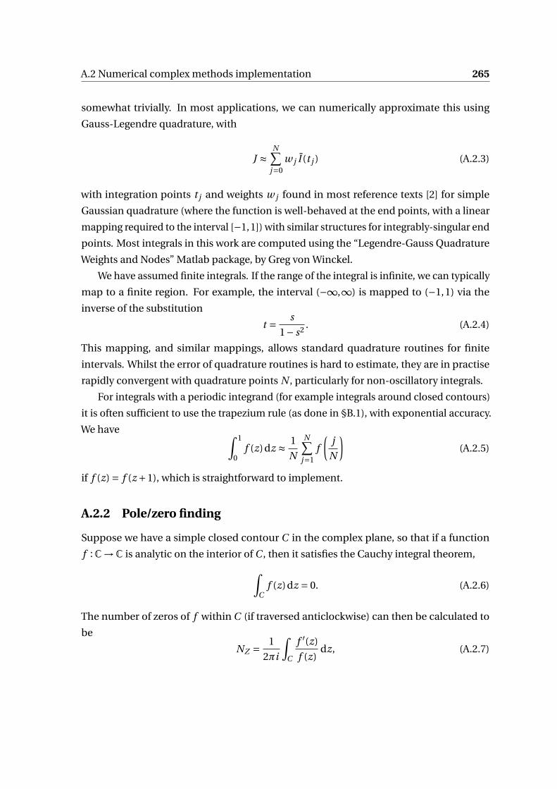
A.2 Numerical complex methods implementation 265

somewhat trivially. In most applications, we can numerically approximate this using

Gauss-Legendre quadrature, with

J ≈N∑

j=0w j I (t j ) (A.2.3)

with integration points t j and weights w j found in most reference texts [2] for simple

Gaussian quadrature (where the function is well-behaved at the end points, with a linear

mapping required to the interval [−1,1]) with similar structures for integrably-singular end

points. Most integrals in this work are computed using the “Legendre-Gauss Quadrature

Weights and Nodes” Matlab package, by Greg von Winckel.

We have assumed finite integrals. If the range of the integral is infinite, we can typically

map to a finite region. For example, the interval (−∞,∞) is mapped to (−1,1) via the

inverse of the substitution

t = s

1− s2. (A.2.4)

This mapping, and similar mappings, allows standard quadrature routines for finite

intervals. Whilst the error of quadrature routines is hard to estimate, they are in practise

rapidly convergent with quadrature points N , particularly for non-oscillatory integrals.

For integrals with a periodic integrand (for example integrals around closed contours)

it is often sufficient to use the trapezium rule (as done in §B.1), with exponential accuracy.

We have ∫ 1

0f (z)dz ≈ 1

N

N∑j=1

f

(j

N

)(A.2.5)

if f (z) = f (z +1), which is straightforward to implement.

A.2.2 Pole/zero finding

Suppose we have a simple closed contour C in the complex plane, so that if a function

f :C→C is analytic on the interior of C , then it satisfies the Cauchy integral theorem,∫C

f (z)dz = 0. (A.2.6)

The number of zeros of f within C (if traversed anticlockwise) can then be calculated to

be

NZ = 1

2πi

∫C

f ′(z)

f (z)dz, (A.2.7)

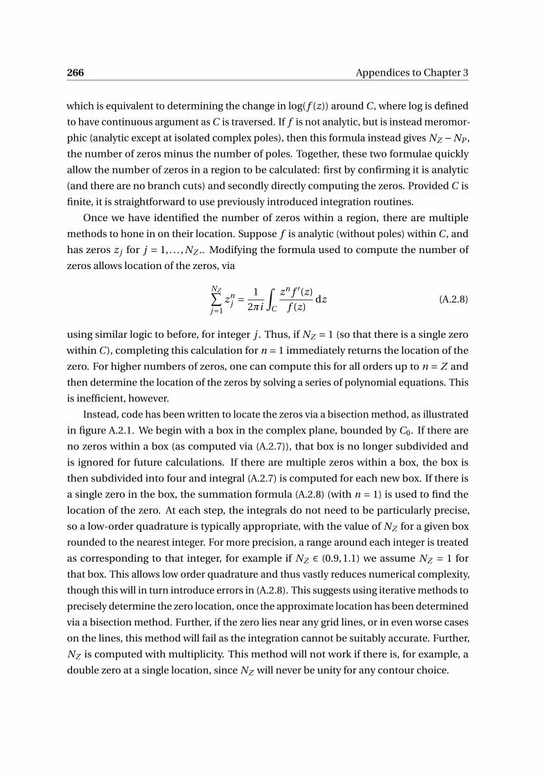
266 Appendices to Chapter 3

which is equivalent to determining the change in log( f (z)) around C , where log is defined

to have continuous argument as C is traversed. If f is not analytic, but is instead meromor-

phic (analytic except at isolated complex poles), then this formula instead gives NZ −NP ,

the number of zeros minus the number of poles. Together, these two formulae quickly

allow the number of zeros in a region to be calculated: first by confirming it is analytic

(and there are no branch cuts) and secondly directly computing the zeros. Provided C is

finite, it is straightforward to use previously introduced integration routines.

Once we have identified the number of zeros within a region, there are multiple

methods to hone in on their location. Suppose f is analytic (without poles) within C , and

has zeros z j for j = 1, . . . , NZ .. Modifying the formula used to compute the number of

zeros allows location of the zeros, via

NZ∑j=1

znj = 1

2πi

∫C

zn f ′(z)

f (z)dz (A.2.8)

using similar logic to before, for integer j . Thus, if NZ = 1 (so that there is a single zero

within C ), completing this calculation for n = 1 immediately returns the location of the

zero. For higher numbers of zeros, one can compute this for all orders up to n = Z and

then determine the location of the zeros by solving a series of polynomial equations. This

is inefficient, however.

Instead, code has been written to locate the zeros via a bisection method, as illustrated

in figure A.2.1. We begin with a box in the complex plane, bounded by C0. If there are

no zeros within a box (as computed via (A.2.7)), that box is no longer subdivided and

is ignored for future calculations. If there are multiple zeros within a box, the box is

then subdivided into four and integral (A.2.7) is computed for each new box. If there is

a single zero in the box, the summation formula (A.2.8) (with n = 1) is used to find the

location of the zero. At each step, the integrals do not need to be particularly precise,

so a low-order quadrature is typically appropriate, with the value of NZ for a given box

rounded to the nearest integer. For more precision, a range around each integer is treated

as corresponding to that integer, for example if NZ ∈ (0.9,1.1) we assume NZ = 1 for

that box. This allows low order quadrature and thus vastly reduces numerical complexity,

though this will in turn introduce errors in (A.2.8). This suggests using iterative methods to

precisely determine the zero location, once the approximate location has been determined

via a bisection method. Further, if the zero lies near any grid lines, or in even worse cases

on the lines, this method will fail as the integration cannot be suitably accurate. Further,

NZ is computed with multiplicity. This method will not work if there is, for example, a

double zero at a single location, since NZ will never be unity for any contour choice.

A.2 Numerical complex methods implementation 267

Fig. A.2.1 Contours for the bisection method, schematically shown in the case of f havingthree zeros (shown by open circles). Integration of (A.2.7) is done recursively, beginningwith the black outer contour, followed by the red division (into quarters), followed bythe blue division (into sixteenths), terminating when the number of zeros in each squareis either one (schematically shown as shaded) or none. All contours are traversed anti-clockwise. In this case, two iterations are enough to broadly identify the location of theouter zero but three are required for the second and third. The closer the zeros, the moreiterations are required to separate them.

Zeros can also be located using the standard Newton-Raphson iteration scheme. If f

and f ′ are both known (potentially computing f ′ numerically via central differences or

better methods) then the iterative scheme

zn+1 = zn − f (zn)

f ′(zn)(A.2.9)

gives a recursive method of finding the zero. If it converges, then it will converge to a zero

of f , even in the complex plane. It does, however, require a good initial guess (which is

where the bisection method is useful for beginning the analysis). If f has multiple zeros

and we have found a single zero z0, then defining

f (z) = f (z)

z − z0(A.2.10)

which is regular at z0, allows repeated application of this and similar methods to find

further zeros.

Typically in this work a coarse bisection method followed by Newton-Raphson will

be used, with the bisection used to obtain an approximate zero location. Alternatively,

it is possible to eyeball zeros of a function by using a phase plot, and using this as an

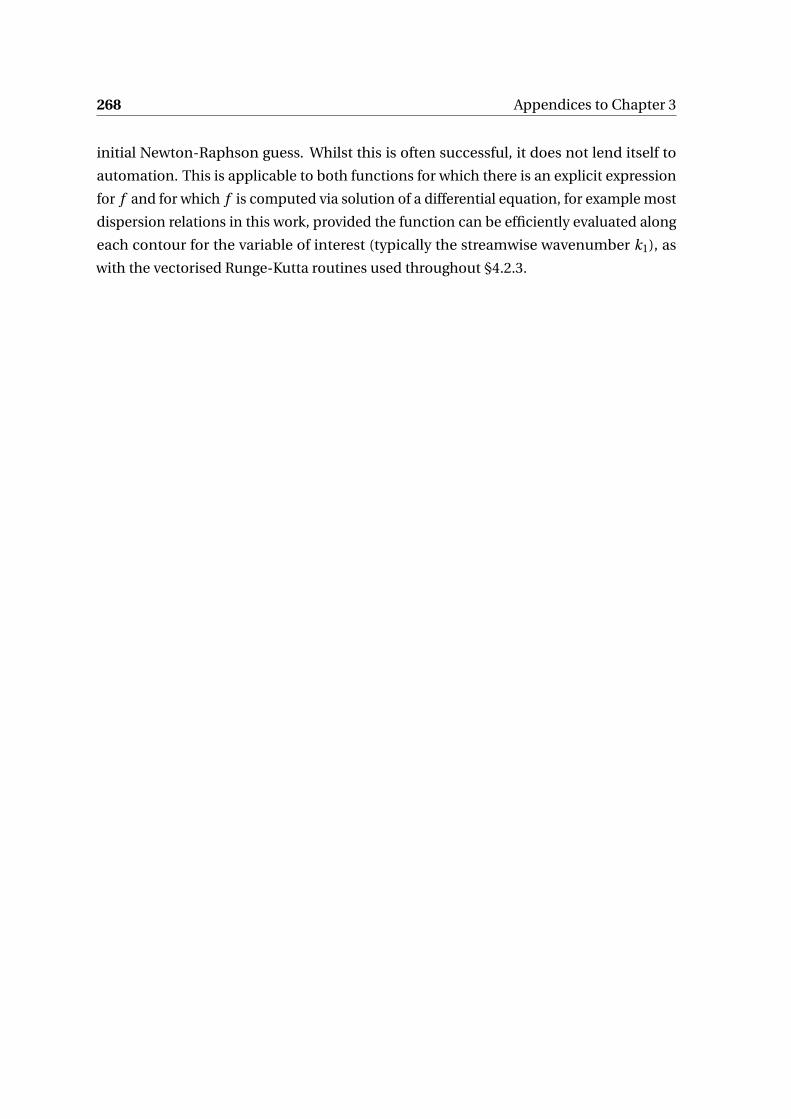
268 Appendices to Chapter 3

initial Newton-Raphson guess. Whilst this is often successful, it does not lend itself to

automation. This is applicable to both functions for which there is an explicit expression

for f and for which f is computed via solution of a differential equation, for example most

dispersion relations in this work, provided the function can be efficiently evaluated along

each contour for the variable of interest (typically the streamwise wavenumber k1), as

with the vectorised Runge-Kutta routines used throughout §4.2.3.

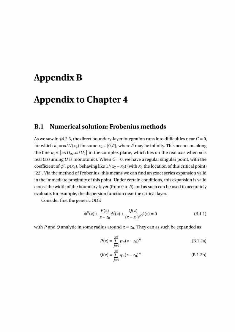
Appendix B

Appendix to Chapter 4

B.1 Numerical solution: Frobenius methods

As we saw in §4.2.3, the direct boundary-layer integration runs into difficulties near C = 0,

for which k1 =ω/U (x2) for some x2 ∈ [0,δ], where δ may be infinity. This occurs on along

the line k1 ∈ [ω/U∞,ω/U0

]in the complex plane, which lies on the real axis when ω is

real (assuming U is monotonic). When C = 0, we have a regular singular point, with the

coefficient of φ′, p(x2), behaving like 1/(x2 −x0) (with x0 the location of this critical point)

[22]. Via the method of Frobenius, this means we can find an exact series expansion valid

in the immediate proximity of this point. Under certain conditions, this expansion is valid

across the width of the boundary-layer (from 0 to δ) and as such can be used to accurately

evaluate, for example, the dispersion function near the critical layer.

Consider first the generic ODE

φ′′(z)+ P (z)

z − z0φ′(z)+ Q(z)

(z − z0)2φ(z) = 0 (B.1.1)

with P and Q analytic in some radius around z = z0. They can as such be expanded as

P (z) =∞∑

j=0pn(z − z0)n (B.1.2a)

Q(z) =∞∑

j=0qn(z − z0)n (B.1.2b)

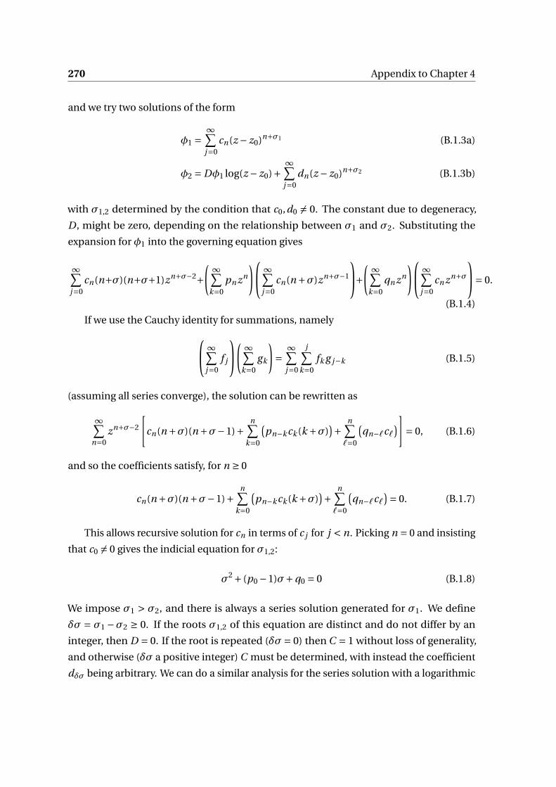
270 Appendix to Chapter 4

and we try two solutions of the form

φ1 =∞∑

j=0cn(z − z0)n+σ1 (B.1.3a)

φ2 = Dφ1 log(z − z0)+∞∑

j=0dn(z − z0)n+σ2 (B.1.3b)

with σ1,2 determined by the condition that c0,d0 = 0. The constant due to degeneracy,

D, might be zero, depending on the relationship between σ1 and σ2. Substituting the

expansion for φ1 into the governing equation gives

∞∑j=0

cn(n+σ)(n+σ+1)zn+σ−2+( ∞∑

k=0pn zn

) ∞∑j=0

cn(n +σ)zn+σ−1

+( ∞∑k=0

qn zn

) ∞∑j=0

cn zn+σ= 0.

(B.1.4)

If we use the Cauchy identity for summations, namely ∞∑j=0

f j

( ∞∑k=0

gk

)=

∞∑j=0

j∑k=0

fk g j−k (B.1.5)

(assuming all series converge), the solution can be rewritten as

∞∑n=0

zn+σ−2

[cn(n +σ)(n +σ−1)+

n∑k=0

(pn−k ck (k +σ)

)+ n∑ℓ=0

(qn−ℓcℓ

)]= 0, (B.1.6)

and so the coefficients satisfy, for n ≥ 0

cn(n +σ)(n +σ−1)+n∑

k=0

(pn−k ck (k +σ)

)+ n∑ℓ=0

(qn−ℓcℓ

)= 0. (B.1.7)

This allows recursive solution for cn in terms of c j for j < n. Picking n = 0 and insisting

that c0 = 0 gives the indicial equation for σ1,2:

σ2 + (p0 −1)σ+q0 = 0 (B.1.8)

We impose σ1 > σ2, and there is always a series solution generated for σ1. We define

δσ = σ1 −σ2 ≥ 0. If the roots σ1,2 of this equation are distinct and do not differ by an

integer, then D = 0. If the root is repeated (δσ= 0) then C = 1 without loss of generality,

and otherwise (δσ a positive integer) C must be determined, with instead the coefficient

dδσ being arbitrary. We can do a similar analysis for the series solution with a logarithmic

B.1 Numerical solution: Frobenius methods 271

term. For n = 0 to σ1 −σ2 −1, the coefficients dn satisfy (B.1.7), unchanged. This then

allows computation of C as

D =−∑δσ−1

j=0 d j pδσ− j ( j +σ2)+∑δσ−1j=0 d j qδσ− j

c0(2σ1 −1)+ c0p0. (B.1.9)

This requires setting dδσ = 0. This is allowed, as choice of a different constant merely

reproduces a multiple of the already determined φ1. The remaining coefficients dn can

then be determined from evaluating the higher-order terms, noting the contribution from

cn . Explicitly, we have

cn =−∑n−1

j=0 c j pn− j (σ1 + j )+∑n−1j=0 c j qn− j

(n +σ1)(n +σ1 −1)+p0(n +σ1)+q0(B.1.10)

dn =−∑n−1

j=0 d j pn− j (σ2 + j )+∑n−1j=0 d j qn− j +D

(∑n−δσj=0 c j pn−δσ− j + cn−δσ(2n +2σ2 −1)

)(n +σ2)(n +σ2 −1)+p0(n +σ2)+q0

(B.1.11)

with sums understood to vanish if the upper limit of summation is less than than the

lower limit. These are straightforward to implement algorithmically, being sums and

products of known numbers, providing a rapid polynomial approximation of the solution

to high-order rapidly.

B.1.1 Computation of Taylor/Laurent coefficients

We have assumed that we know expansions of P and Q in powers of (z − z0). This is

equivalent to knowing Laurent expansions of p(z) = P (z)/(z − z0) and q(z) = Q(z)/(z −z0)2, which links to the formulation described earlier. In both cases, robust numerical

implementation of Cauchy’s integral formula exist when p and q are defined (locally) in

the complex plane about z0 [17]. Suppose a function p has the Laurent expansion (wlog

around z0 = 0)

p(z) =∞∑

j=−Np j z j (B.1.12)

where N might be infinity, but for the purposes of this exercise is a finite integer. The

coefficients are then explicitly given by

p j = 1

2πi

∫γ

p(z)

z j+1dz (B.1.13)

272 Appendix to Chapter 4

with γ a simple closed contour containing z = 0, traversed anticlockwise, with p(z) analytic

(z = 0 aside) on the interior of the contour.

Picking the contour to be the unit circle |z| = R, the symmetry and periodic nature of

the integral allows accurate discretation of this integral as

p j ≈ 1

mRn

m=1∑j=0

p(Re2πi j /m)e−2nπi j /m (B.1.14)

with R and m chooseable parameters. Whilst it might seem choosing R as small as possible

(evaluating as close as possible to the singularity) is appropriate for accuracy, it can be

seen the leading factor of R−n amplifies numerical errors (for example, if the integral is

smaller than machine error) for higher n, and as such it makes sense to choose R = 1 or

larger if possible, that is if p has no other singularities within this radius.

This is often the most numerically challenging part of the exercise, particularly if

the ODE depends on some parameter k. Ideally, these coefficients should be computed

analytically where possible. For the incompressible Rayleigh equation, this is possible if

an analytic expression for U and c0 exists, however numerical methods remove the need

to vary the routine with the choice of background flow, which is useful for the construction

of generic numerical routines.

B.1.2 Construction of ODE solutions, and range of validity

We have two solutions φ1 and φ2 that form a basis for the solutions to the differential

equation in some region around z0. If we look for a specific solution φ that satisfies some

conditions at a point z = δ, with φ(δ) =α and φ′(δ) =β, then

φ= φ′2(δ)α−φ2(δ)β

φ1(δ)φ′2(δ)−φ2(δ)φ′

1(δ)φ1(z)+ φ′

1(δ)α+φ1(δ)β

φ1(δ)φ′2(δ)−φ2(δ)φ′

1(δ)φ2(z) (B.1.15)

with series expressions avaliable for φ j and φ′j .

This assumes that z0 −δ is within the radius of convergence for the power series

solutions, which is the same as the radius of convergence for the series expansions of p

and q : that is, there is no other singular points within a circle of radius |z0 −δ| around

z0. If we want a solution valid across the boundary-layer, from z = 0 to z = δ, we require

|z0|, |z0−δ| < |z0−z0 j | for all j , with z0 j the set of singularities of p and q away from z = z0.

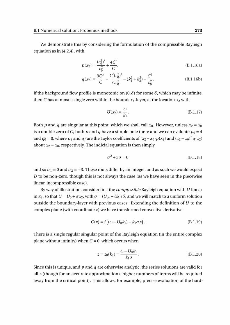
B.1 Numerical solution: Frobenius methods 273

We demonstrate this by considering the formulation of the compressible Rayleigh

equation as in (4.2.4), with

p(x2) = (c20)′

c20

+ 4C ′

C, (B.1.16a)

q(x2) = 3C ′′

C+ C ′(c2

0)′

C c20

− (k21 +k2

3)− C 2

c20

. (B.1.16b)

If the background flow profile is monotonic on (0,δ) for some δ, which may be infinite,

then C has at most a single zero within the boundary-layer, at the location x2 with

U (x2) = ω

k1. (B.1.17)

Both p and q are singular at this point, which we shall call x0. However, unless x2 = x0

is a double zero of C , both p and q have a simple pole there and we can evaluate p0 = 4

and q0 = 0, where p j and q j are the Taylor coefficients of (x2−x0)p(x2) and (x2−x0)2q(x2)

about x2 = x0, respectively. The indicial equation is then simply

σ2 +3σ= 0 (B.1.18)

and so σ1 = 0 and σ2 =−3. These roots differ by an integer, and as such we would expect

D to be non-zero, though this is not always the case (as we have seen in the piecewise

linear, incompressible case).

By way of illustration, consider first the compressible Rayleigh equation with U linear

in x2, so that U =U0+σx2, with σ= (U∞−U0)/δ, and we will match to a uniform solution

outside the boundary-layer with previous cases. Extending the definition of U to the

complex plane (with coordinate z) we have transformed convective derivative

C (z) = i((ω−U0k1)−k1σz

). (B.1.19)

There is a single regular singular point of the Rayleigh equation (in the entire complex

plane without infinity) when C = 0, which occurs when

z = z0(k1) = ω−U0k1

k1σ. (B.1.20)

Since this is unique, and p and q are otherwise analytic, the series solutions are valid for

all z (though for an accurate approximation a higher numbers of terms will be required

away from the critical point). This allows, for example, precise evaluation of the hard-

274 Appendix to Chapter 4

;

0 0.1 0.2 0.3 0.4 0.5 0.6 0.7 0.8 0.9 1

−15

−10

−5

0

x2

log 10

|φd

,N−φ

d,C| N = 3

N = 5N = 7N = 9N = 11N = 13N = 15

Fig. B.1.1 Considering a linear profile with U0 = 0.5 and U∞ = 1, scaling lengths with δ∞.The background speed of sound is constant, c0 = 2, and frequencyω= 1. For k1 = 1.5+0.1i ,near and above the critical layer, the decaying solution is computed via a series method,truncating sums after N terms. This is compared to the integrated solution with stepsize 1×10−4, and (the logarithm of) their difference plotted across the boundary-layer(so both functions fixed identical at x2 = 1). Error rapidly decreases with N . For largeN , the apparent error is most likely caused by the error in the alternative method fromintegrating over the boundary-layer, and is more pronounced near the critical point. Theseries solution is very accurate even for N small, with an absolute error of around 5% inthe smallest possible case N = 3.

wall dispersion function Dh(k1) in the vicinity of the critical-layer (which contains all k1

such that z0(k1) is real and lies between 0 and δ), which can be compared to the directly

integrated solution and demonstrates the accuracy of this method near the critical-layer,

see figures B.1.1 and B.1.2a. The method is particularly precise near the slipping edge of

the critical layer, with k1 ≈ω/U0. In the linear case there is not actually a branch cut along

where the critical-layer would be, but the Frobenius method highlights the root of the

dispersion relation on the real axis.

The critical-layer forms a natural branch-cut in the complex plane, which masks what

is happening along the cut itself. This method allows choice of direction of this branch

cut, through the log term [22], which allows isolation of the zero of the dispersion of

this critical-layer in this case (though, as we can see, the critical-layer is removable if the

background profile is linear and there is no geometry). This is similar to the deformation

of the critical-layer seen when numerically integrating along a complex contour, as in the

next section and, for example, figure 4.2.7.

We have established that this method is effective in the case of a linear profile, extend-

ing the long-wavelength analysis somewhat. What happens, however, if the background

profile has some variation in shear? We consider first the simplest case of a parabolic

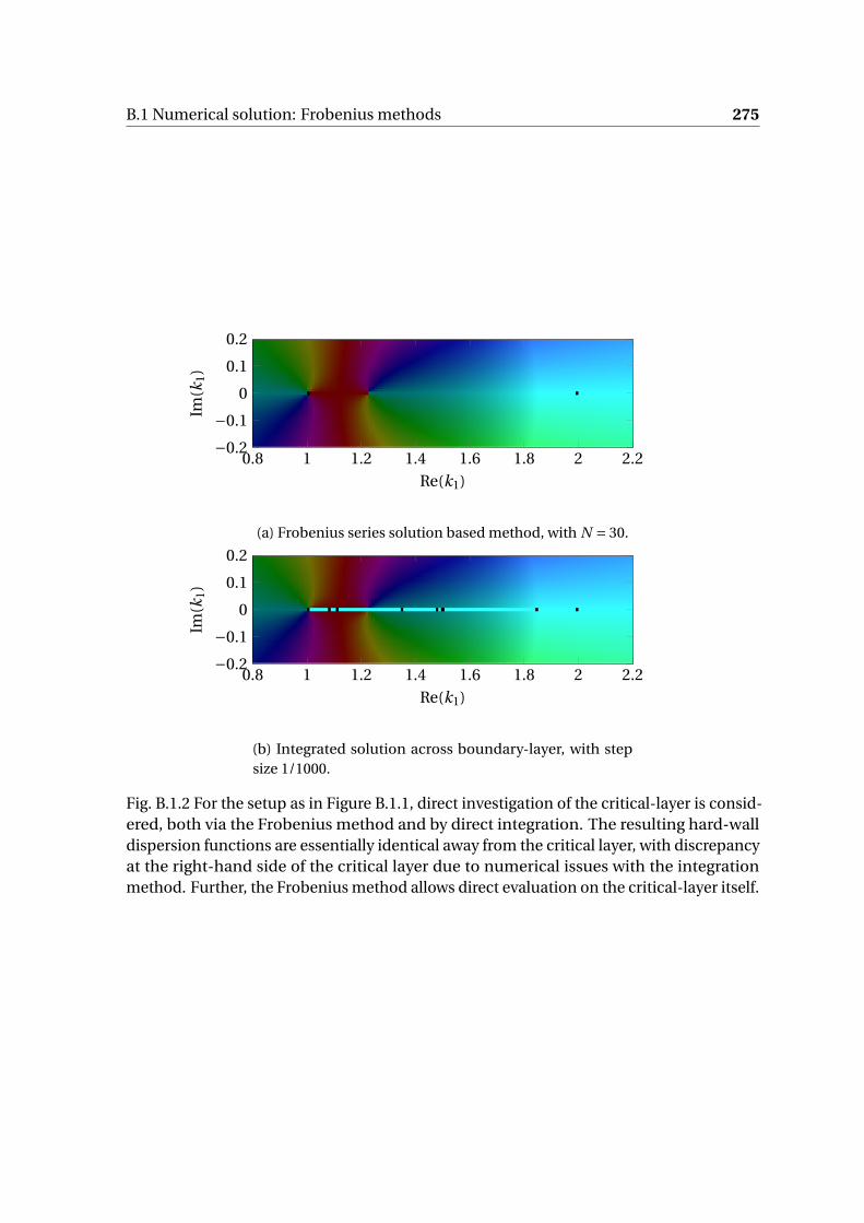
B.1 Numerical solution: Frobenius methods 275

0.8 1 1.2 1.4 1.6 1.8 2 2.2−0.2

−0.1

0

0.1

0.2

Re(k1)

Im(k

1)

(a) Frobenius series solution based method, with N = 30.

0.8 1 1.2 1.4 1.6 1.8 2 2.2−0.2

−0.1

0

0.1

0.2

Re(k1)

Im(k

1)

(b) Integrated solution across boundary-layer, with stepsize 1/1000.

Fig. B.1.2 For the setup as in Figure B.1.1, direct investigation of the critical-layer is consid-ered, both via the Frobenius method and by direct integration. The resulting hard-walldispersion functions are essentially identical away from the critical layer, with discrepancyat the right-hand side of the critical layer due to numerical issues with the integrationmethod. Further, the Frobenius method allows direct evaluation on the critical-layer itself.

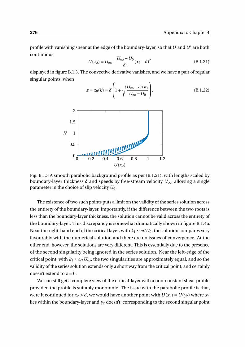
276 Appendix to Chapter 4

profile with vanishing shear at the edge of the boundary-layer, so that U and U ′ are both

continuous:

U (x2) =U∞+ U∞−U0

δ2(x2 −δ)2 (B.1.21)

displayed in figure B.1.3. The convective derivative vanishes, and we have a pair of regular

singular points, when

z = z0(k) = δ1∓

√U∞−ω/k1

U∞−U0

. (B.1.22)

0 0.2 0.4 0.6 0.8 1 1.20

0.5

1

1.5

2

U (x2)

x 2

Fig. B.1.3 A smooth parabolic background profile as per (B.1.21), with lengths scaled byboundary-layer thickness δ and speeds by free-stream velocity U∞, allowing a singleparameter in the choice of slip velocity U0.

The existence of two such points puts a limit on the validity of the series solution across

the entirety of the boundary-layer. Importantly, if the difference between the two roots is

less than the boundary-layer thickness, the solution cannot be valid across the entirety of

the boundary-layer. This discrepancy is somewhat dramatically shown in figure B.1.4a.

Near the right-hand end of the critical layer, with k1 ∼ω/U0, the solution compares very

favourably with the numerical solution and there are no issues of convergence. At the

other end, however, the solutions are very different. This is essentially due to the presence

of the second singularity being ignored in the series solution. Near the left-edge of the

critical point, with k1 ≈ω/U∞, the two singularities are approximately equal, and so the

validity of the series solution extends only a short way from the critical point, and certainly

doesn’t extend to z = 0.

We can still get a complete view of the critical-layer with a non-constant shear profile

provided the profile is suitably monotonic. The issue with the parabolic profile is that,

were it continued for x2 > δ, we would have another point with U (x2) =U (y2) where x2

lies within the boundary-layer and y2 doesn’t, corresponding to the second singular point

B.1 Numerical solution: Frobenius methods 277

for fixed k1. If this second point z01 is suitably far away, |z0 − z01| > δ, then the series

solution converges across the entirety of the boundary-layer. For this purpose, consider

the parabolic background profile U (x2) satisfying U (δ j ) =U j with δ = (δ0,δ1,δ∞), U =(U0,U1,U∞), given by

U (x2) =U0 + A(x2 −δ0)+B(x2 −δ0)2 (B.1.23)

with

B = 1

δ∞−δ1

(U∞−U0

δ∞−U0− U1 −U0

δ1 −δ0

)(B.1.24a)

A = U1 −U0

δ1 −δ0−Cδ1 (B.1.24b)

and corresponding singular points (zeros of C ):

z0(k) = −A+√

A2 −4B(U0 −ω/k1)

2B, (B.1.25a)

z01(k) = −B −√

A2 −4B(U0 −ω/k1)

2B. (B.1.25b)

These poles are suitably separated for convergence

A2 −4B(U0 −U∞) > B 2δ2. (B.1.26)

The accuracy of the Frobenius series solution, provided this condition holds, for a profile

with small shear variation (so that U ′′ is small) is shown in figure B.1.4b. As seen before,

where there is convergence of the series solution we gain a far greater degree of accuracy

near, and on, the critical-layer.

278 Appendix to Chapter 4

0.8 1 1.2 1.4 1.6 1.8 2 2.2−0.2

−0.1

0

0.1

0.2

Re(k1)

Im(k

1)

(a) Parabolic profile with continuous derivative at free-stream boundary, with U (0) = 0.5

0.8 1 1.2 1.4 1.6 1.8 2 2.2−0.2

−0.1

0

0.1

0.2

Re(k1)

Im(k

1)

(b) Parabolic profile with U (0) = 0.5, U (0.5) = 0.8.

Fig. B.1.4 Phase plot of the ratio of hard-wall dispersion functions, Dh,computed/Dh,frobenius,with the red colour on the right of the plot indicating agreement. The black and speckledregions indicate areas where the Frobenius solution does not converge sufficiently. Inboth cases, lengths are scaled by boundary-layer thickness δ and speeds by U∞, withc0 = 2 throughout. The region of agreement with the numerics is much greater for thesecond case, where the "hidden" singular point is further from the region x2 ∈ (0,δ) forpoints near this critical-layer branch cut, though neither case has a successful evaluationof the dispersion function near k1 =ω/U∞, the "free-stream" wavenumber.