Acoustic robot navigation using distributed microphone arrays

Information Fusion 5 (2004) 131–140

www.elsevier.com/locate/inffus

Acoustic robot navigation using distributed microphone arrays

Qing Hua Wang, Teodor Ivanov, Parham Aarabi *

Electrical and Computer Engineering, University of Toronto, 10 Kings College Road, Toronto, Canada M5S3G4

Received 22 July 2003; received in revised form 15 October 2003; accepted 15 October 2003

Abstract

This paper presents a method for the navigation of a mobile robot using sound localization in the context of a robotic lab tour

guide. Sound localization, which is achieved using an array of 24 microphones distributed on two walls of the lab, is performed

whenever the robot speaks as part of the tour. The SRP-PHAT sound localization algorithm is used to estimate the current location

of the robot using approximately 2 s of recorded signal. Navigation is achieved using several stops during which the estimated

location of the robot is used to make course adjustments. Experiments using the acoustic robot navigation system illustrate the

accuracy of the proposed technique, which resulted in an average localization error of about 7 cm close to the array and 30 cm far

away from the array.

� 2003 Elsevier B.V. All rights reserved.

Keywords: Robot navigation; Sound localization; Microphone arrays

1. Introduction

Numerous applications exist for mobile robots

capable of exploring and navigating through their

environment. They can be deployed in hazardous envi-ronments like mines and chemically contaminated

buildings, which are too dangerous for human intrusion.

They can and have been used in the exploration of new

or otherwise inaccessible environments like other plan-

ets. They can also be used in tasks such as conducting

guided tours of museums or laboratories. All of these

applications rely heavily on an accurate navigation

system, which in turn requires accurate estimations ofthe position of the robot. Once this information is

known, it is possible to plot a path between two or more

points, or even to find a course for an articulated robot

in a tightly spaced environment [17].

A wide variety of robot localization algorithms have

been explored in the past. A commonly applied method

makes use of electromagnetic beacons, which are de-

tected by the robot and used for localization [15,18].A robot localization technique that utilized environ-

mental landmarks was discussed by [19]. This system

required bearing measurements from the robot to three

*Corresponding author. Tel.: +1-416-9467893; fax: +1-416-

9784425.

E-mail address: [email protected] (P. Aarabi).

1566-2535/$ - see front matter � 2003 Elsevier B.V. All rights reserved.

doi:10.1016/j.inffus.2003.10.002

or more landmarks in order to perform robot localiza-

tion. Additional hardware, such as unspecified bearing

sensors were required to localize the robot from land-

mark information.

Vision-based localization represents another com-monly applied solution to the problem. One such

example is the technique of [6], which used cameras

mounted on the robot to capture landmark images and

compared them to a prior landmark map. The tech-

niques of [9,11] present two other examples of vision-

based robot localization. The technique used by [9] took

brightness measurements of the ceiling using a vertically

mounted camera, knowledge of the robot’s motion, anda base map of the entire environment’s ceiling brightness

in order to calculate the robot’s position. The vision-

based technique proposed by [11] used a neural network

trained with a set of sample images in the environment

in order to determine the robot’s position from camera

images. A similar technique involving visual landmarks

proposed by [20] combines the benefits of vision-based

and landmark-based localization. Each of these vision-based localization methods brings certain solutions to

the robot localization problem, but all require addi-

tional computation and hardware onboard the robot.

The ultrasonic sensor-based localization method

presented by [12] employed a set of ultrasonic sensors in

a ring configuration to create a map of the environment,

which was then compared with a prior environment

mail to: [email protected]

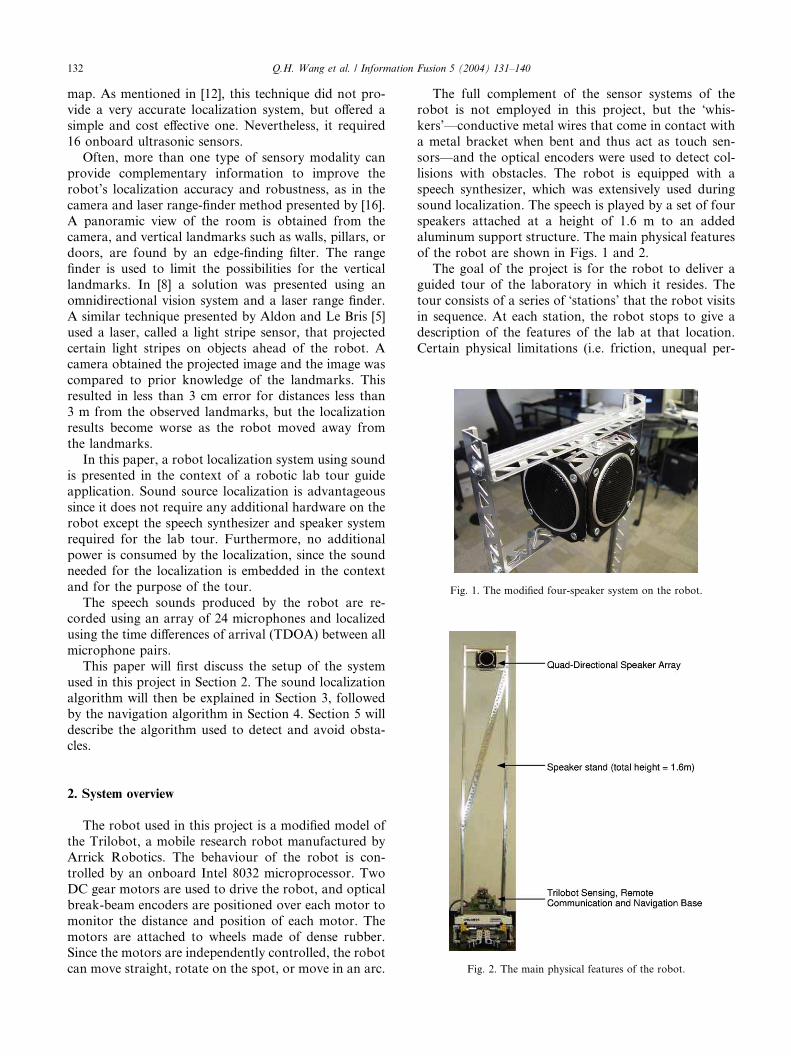
Fig. 1. The modified four-speaker system on the robot.

132 Q.H. Wang et al. / Information Fusion 5 (2004) 131–140

map. As mentioned in [12], this technique did not pro-vide a very accurate localization system, but offered a

simple and cost effective one. Nevertheless, it required

16 onboard ultrasonic sensors.

Often, more than one type of sensory modality can

provide complementary information to improve the

robot’s localization accuracy and robustness, as in the

camera and laser range-finder method presented by [16].

A panoramic view of the room is obtained from thecamera, and vertical landmarks such as walls, pillars, or

doors, are found by an edge-finding filter. The range

finder is used to limit the possibilities for the vertical

landmarks. In [8] a solution was presented using an

omnidirectional vision system and a laser range finder.

A similar technique presented by Aldon and Le Bris [5]

used a laser, called a light stripe sensor, that projected

certain light stripes on objects ahead of the robot. Acamera obtained the projected image and the image was

compared to prior knowledge of the landmarks. This

resulted in less than 3 cm error for distances less than

3 m from the observed landmarks, but the localization

results become worse as the robot moved away from

the landmarks.

In this paper, a robot localization system using sound

is presented in the context of a robotic lab tour guideapplication. Sound source localization is advantageous

since it does not require any additional hardware on the

robot except the speech synthesizer and speaker system

required for the lab tour. Furthermore, no additional

power is consumed by the localization, since the sound

needed for the localization is embedded in the context

and for the purpose of the tour.

The speech sounds produced by the robot are re-corded using an array of 24 microphones and localized

using the time differences of arrival (TDOA) between all

microphone pairs.

This paper will first discuss the setup of the system

used in this project in Section 2. The sound localization

algorithm will then be explained in Section 3, followed

by the navigation algorithm in Section 4. Section 5 will

describe the algorithm used to detect and avoid obsta-cles.

Fig. 2. The main physical features of the robot.

2. System overview

The robot used in this project is a modified model of

the Trilobot, a mobile research robot manufactured by

Arrick Robotics. The behaviour of the robot is con-

trolled by an onboard Intel 8032 microprocessor. Two

DC gear motors are used to drive the robot, and optical

break-beam encoders are positioned over each motor to

monitor the distance and position of each motor. The

motors are attached to wheels made of dense rubber.Since the motors are independently controlled, the robot

can move straight, rotate on the spot, or move in an arc.

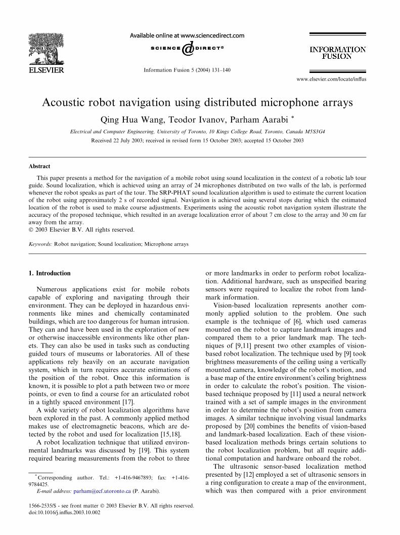
The full complement of the sensor systems of therobot is not employed in this project, but the �whis-kers’––conductive metal wires that come in contact with

a metal bracket when bent and thus act as touch sen-

sors––and the optical encoders were used to detect col-

lisions with obstacles. The robot is equipped with a

speech synthesizer, which was extensively used during

sound localization. The speech is played by a set of four

speakers attached at a height of 1.6 m to an addedaluminum support structure. The main physical features

of the robot are shown in Figs. 1 and 2.

The goal of the project is for the robot to deliver a

guided tour of the laboratory in which it resides. The

tour consists of a series of �stations’ that the robot visitsin sequence. At each station, the robot stops to give a

description of the features of the lab at that location.

Certain physical limitations (i.e. friction, unequal per-

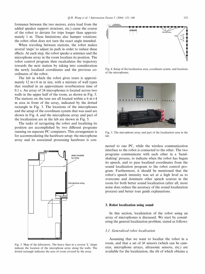
Microphones

0.2m

Walls

(0,0)x-direction

y-di

rect

ion

Fig. 4. Setup of the localization area, coordinate system, and locations

of the microphones.

Fig. 5. The microphone array and part of the localization area in the

lab.

Q.H. Wang et al. / Information Fusion 5 (2004) 131–140 133

formance between the two motors, extra load from theadded speaker support structure, etc.) cause the course

of the robot to deviate for trips longer than approxi-

mately 1 m. These limitations also hamper rotations:

the robot often does not turn the exact angle intended.

When traveling between stations, the robot makes

several �steps’ to adjust its path in order to reduce these

effects. At each step, the robot speaks a sentence and the

microphone array in the room localizes its position. Therobot control program then recalculates the trajectory

towards the next station by taking into consideration

the newly localized coordinates and the previous co-

ordinates of the robot.

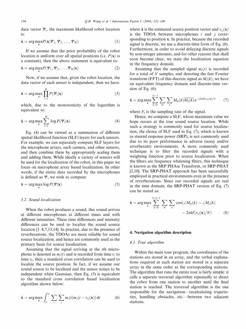
The lab in which the robot gives tours is approxi-

mately 12 m · 6 m in size, with a mixture of wall types

that resulted in an approximate reverberation time of

0.1 s. An array of 24 microphones is located across twowalls in the upper half of the room, as shown in Fig. 3.

The stations on the tour are all located within a 6 m · 4m area in front of the array, indicated by the dotted

rectangle in Fig. 3. The locations of the microphones

and the setup of the coordinate system that was used are

shown in Fig. 4, and the microphone array and part of

the localization are in the lab are shown in Fig. 5.

The tasks of navigating the robot and localizing itsposition are accomplished by two different programs

running on separate PC computers. This arrangement is

for accommodating the hardware setup: the microphone

array and its associated processing hardware is con-

Fig. 3. Map of the laboratory. The heavy lines in a reverse �L’ shapeindicate the location of the microphone array along the walls. The

dotted rectangle indicates the area of room covered by the array.

nected to one PC, while the wireless communication

interface to the robot is connected to the other. The two

programs communicate with each other in a �hand-shaking’ process, to indicate when the robot has begun

its speech, and to pass localized coordinates from the

sound localization program to the robot control pro-

gram. Furthermore, it should be mentioned that the

robot’s speech intensity was set at a high level as toovercome and dominate other speech sources in the

room for both better sound localization (after all, more

noise does reduce the accuracy of the sound localization

process) and better tour guide explanations.

3. Robot localization using sound

In this section, localization of the robot using an

array of microphones is discussed. We start by consid-

ering the general localization problem, stated as follows:

3.1. Generalized robot localization

Assuming that we want to localize the robot in a

room, and that a set of M sensors (which can be cam-eras, microphone arrays, ultrasonic sensors, etc.) are

available for the localization, the ith of which obtains a


data vector Wi, the maximum likelihood robot locationis:

~x ¼ argmaxx

P ðxjW1;W2; . . . ;WMÞ ð1Þ

If we assume that the prior probability of the robot

location is uniform over all spatial positions (i.e. P ðxÞ isa constant), then the above statement is equivalent to:

~x ¼ argmaxx

P ðW1;W2; . . . ;WM jxÞ ð2Þ

Now, if we assume that, given the robot location, the

data vector of each sensor is independent, then we have:

~x ¼ argmaxx

YMi¼1

P ðWijxÞ ð3Þ

which, due to the monotonicity of the logarithm is

equivalent to:

~x ¼ argmaxx

XMi¼1

log PðWijxÞ ð4Þ

Eq. (4) can be viewed as a summation of different

spatial likelihood function (SLF) layers for each sensors.

For example, we can separately compute SLF layers for

the microphone arrays, each camera, and other sensors,

and then combine them by appropriately scaling themand adding them. While ideally a variety of sensors will

be used for the localization of the robot, in this paper we

focus on microphone array based localization. In other

words, if the entire data recorded by the microphones

is defined as W, we wish to compute:

~x ¼ argmaxx

log P ðWjxÞ ð5Þ

3.2. Sound localization

When the robot produces a sound, this sound arrives

at different microphones at different times and with

different intensities. These time differences and intensity

differences can be used to localize the sound source

location [1–4,7,13,14]. In practice, due to the presence ofreverberations, the TDOAs are more reliable for sound

source localization, and hence are commonly used as the

primary basis for source localization.

Assuming that the signal arriving at the ith micro-

phone is denoted as miðtÞ and is recorded from time t1 totime t2, then a standard cross correlation can be used to

localize the source position. In fact, if we assume our

sound source to be localized and the sensor noises to beindependent white Gaussian, then Eq. (5) is equivalent

to the standard cross correlation based localization

algorithm shown below:

~x ¼ argmaxx

Z t2

t1

Xi

Xj

miðtÞmjðt � sijðxÞÞdt ð6Þ

where ~x is the estimated source position vector and sijðxÞis the TDOA between microphones i and j corre-

sponding to position x. In practice, because the recorded

signal is discrete, we use a discrete-time form of Eq. (6).

Furthermore, in order to avoid delaying discrete signals

by non-integer amounts, and for other reasons that shall

soon become clear, we state the localization equation

in the frequency domain.

Assuming that the sampled signal miðtÞ is recordedfor a total of N samples, and denoting the fast Fourier

transform (FFT) of this discrete signal as MiðkÞ, we havean equivalent frequency domain and discrete-time ver-

sion of Eq. (6):

~x ¼ argmaxx

XN�1

k¼0

Xm

Xn

MmðkÞMnðkÞe�j2pkFssijðxÞ=N ð7Þ

where Fs is the sampling rate of the signal.

Hence, we compute a SLF, whose maximum value we

hope occurs at the true sound source location. While

such a strategy is commonly used for source localiza-

tion, the choice of SLF used in Eq. (7), which is knownas steered response power (SRP), is not commonly used

due to its poor performance in adverse (noisy and/or

reverberant) environments. A more commonly used

technique is to filter the recorded signals with a

weighting function prior to source localization. When

the filters are frequency whitening filters, this technique

is known as the SRP PHAse Transform, or SRP-PHAT

[2,10]. The SRP-PHAT approach has been successfullyemployed in practical environments even in the presence

of reverberations. Since our recorded signals are real

in the time domain, the SRP-PHAT version of Eq. (7)

can be stated as:

~x ¼ argmaxx

XN=2�1

k¼0

Xm

Xn

cosð\MmðkÞ � \MnðkÞ

� 2pkFssijðxÞ=NÞ ð8Þ

4. Navigation algorithm description

4.1. Tour algorithm

Within the main tour program, the coordinates of thestations are stored in an array, and the verbal explana-

tions required at each station are stored in a separate

array in the same order as the corresponding stations.

The algorithm that runs the entire tour is fairly simple: it

calls a separate traversal algorithm repeatedly to direct

the robot from one station to another until the final

station is reached. The traversal algorithm is the one

responsible for the navigation––recalculating trajecto-ries, handling obstacles, etc.––between two adjacent

stations.

Microphones

Walls

(0,0)x-direction

y-di

rect

ion

(1.5, 1.5)

(3.6, 3.5)

Station 1, Station 3

Station 2

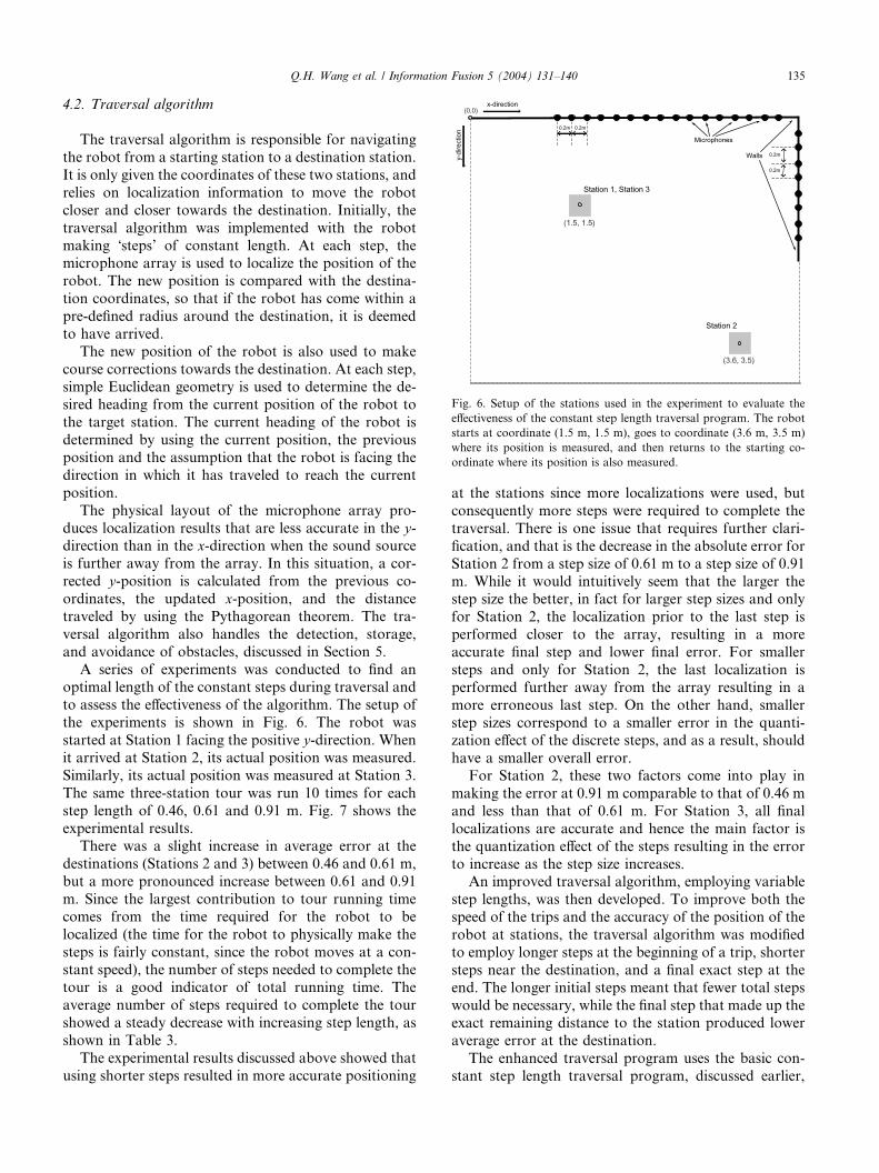
Fig. 6. Setup of the stations used in the experiment to evaluate the

effectiveness of the constant step length traversal program. The robot

starts at coordinate (1.5 m, 1.5 m), goes to coordinate (3.6 m, 3.5 m)

where its position is measured, and then returns to the starting co-

ordinate where its position is also measured.


4.2. Traversal algorithm

The traversal algorithm is responsible for navigating

the robot from a starting station to a destination station.

It is only given the coordinates of these two stations, and

relies on localization information to move the robot

closer and closer towards the destination. Initially, the

traversal algorithm was implemented with the robot

making �steps’ of constant length. At each step, themicrophone array is used to localize the position of the

robot. The new position is compared with the destina-

tion coordinates, so that if the robot has come within a

pre-defined radius around the destination, it is deemed

to have arrived.

The new position of the robot is also used to make

course corrections towards the destination. At each step,

simple Euclidean geometry is used to determine the de-sired heading from the current position of the robot to

the target station. The current heading of the robot is

determined by using the current position, the previous

position and the assumption that the robot is facing the

direction in which it has traveled to reach the current

position.

The physical layout of the microphone array pro-

duces localization results that are less accurate in the y-direction than in the x-direction when the sound source

is further away from the array. In this situation, a cor-

rected y-position is calculated from the previous co-

ordinates, the updated x-position, and the distance

traveled by using the Pythagorean theorem. The tra-

versal algorithm also handles the detection, storage,

and avoidance of obstacles, discussed in Section 5.

A series of experiments was conducted to find anoptimal length of the constant steps during traversal and

to assess the effectiveness of the algorithm. The setup of

the experiments is shown in Fig. 6. The robot was

started at Station 1 facing the positive y-direction. When

it arrived at Station 2, its actual position was measured.

Similarly, its actual position was measured at Station 3.

The same three-station tour was run 10 times for each

step length of 0.46, 0.61 and 0.91 m. Fig. 7 shows theexperimental results.

There was a slight increase in average error at the

destinations (Stations 2 and 3) between 0.46 and 0.61 m,

but a more pronounced increase between 0.61 and 0.91

m. Since the largest contribution to tour running time

comes from the time required for the robot to be

localized (the time for the robot to physically make the

steps is fairly constant, since the robot moves at a con-stant speed), the number of steps needed to complete the

tour is a good indicator of total running time. The

average number of steps required to complete the tour

showed a steady decrease with increasing step length, as

shown in Table 3.

The experimental results discussed above showed that

using shorter steps resulted in more accurate positioning

at the stations since more localizations were used, but

consequently more steps were required to complete the

traversal. There is one issue that requires further clari-

fication, and that is the decrease in the absolute error for

Station 2 from a step size of 0.61 m to a step size of 0.91

m. While it would intuitively seem that the larger thestep size the better, in fact for larger step sizes and only

for Station 2, the localization prior to the last step is

performed closer to the array, resulting in a more

accurate final step and lower final error. For smaller

steps and only for Station 2, the last localization is

performed further away from the array resulting in a

more erroneous last step. On the other hand, smaller

step sizes correspond to a smaller error in the quanti-zation effect of the discrete steps, and as a result, should

have a smaller overall error.

For Station 2, these two factors come into play in

making the error at 0.91 m comparable to that of 0.46 m

and less than that of 0.61 m. For Station 3, all final

localizations are accurate and hence the main factor is

the quantization effect of the steps resulting in the error

to increase as the step size increases.An improved traversal algorithm, employing variable

step lengths, was then developed. To improve both the

speed of the trips and the accuracy of the position of the

robot at stations, the traversal algorithm was modified

to employ longer steps at the beginning of a trip, shorter

steps near the destination, and a final exact step at the

end. The longer initial steps meant that fewer total steps

would be necessary, while the final step that made up theexact remaining distance to the station produced lower

average error at the destination.

The enhanced traversal program uses the basic con-

stant step length traversal program, discussed earlier,

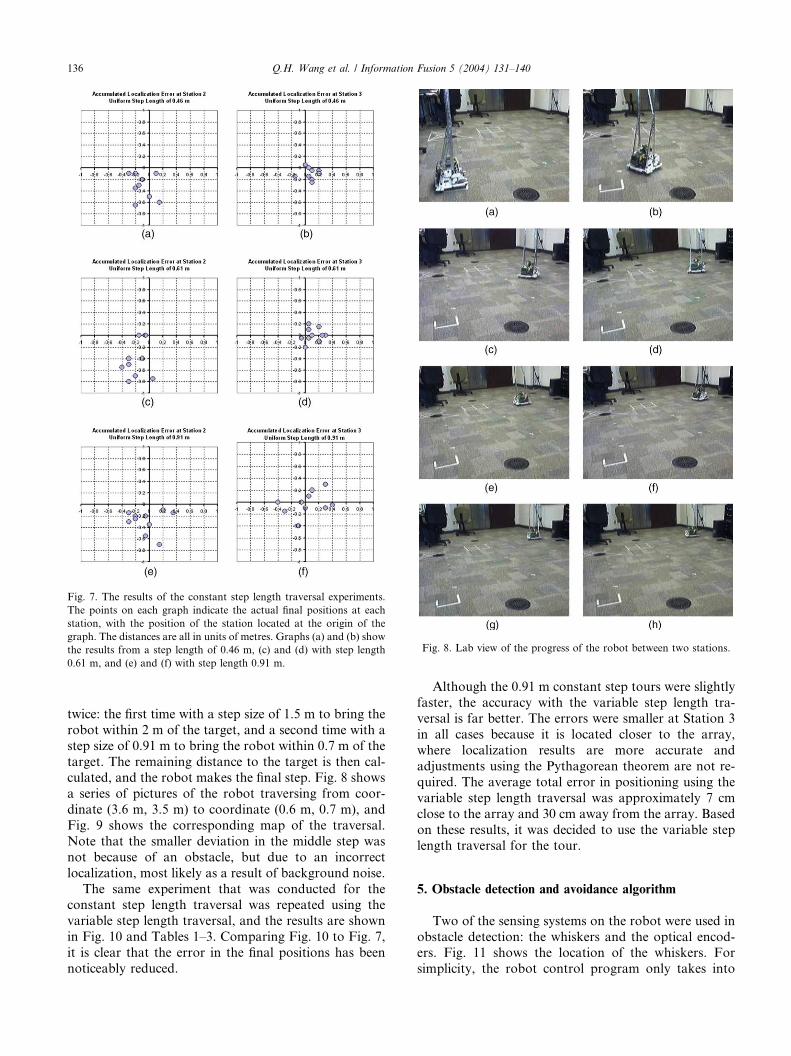
Fig. 7. The results of the constant step length traversal experiments.

The points on each graph indicate the actual final positions at each

station, with the position of the station located at the origin of the

graph. The distances are all in units of metres. Graphs (a) and (b) show

the results from a step length of 0.46 m, (c) and (d) with step length

0.61 m, and (e) and (f) with step length 0.91 m.

Fig. 8. Lab view of the progress of the robot between two stations.


twice: the first time with a step size of 1.5 m to bring the

robot within 2 m of the target, and a second time with a

step size of 0.91 m to bring the robot within 0.7 m of the

target. The remaining distance to the target is then cal-culated, and the robot makes the final step. Fig. 8 shows

a series of pictures of the robot traversing from coor-

dinate (3.6 m, 3.5 m) to coordinate (0.6 m, 0.7 m), and

Fig. 9 shows the corresponding map of the traversal.

Note that the smaller deviation in the middle step was

not because of an obstacle, but due to an incorrect

localization, most likely as a result of background noise.

The same experiment that was conducted for theconstant step length traversal was repeated using the

variable step length traversal, and the results are shown

in Fig. 10 and Tables 1–3. Comparing Fig. 10 to Fig. 7,

it is clear that the error in the final positions has been

noticeably reduced.

Although the 0.91 m constant step tours were slightly

faster, the accuracy with the variable step length tra-versal is far better. The errors were smaller at Station 3

in all cases because it is located closer to the array,

where localization results are more accurate and

adjustments using the Pythagorean theorem are not re-

quired. The average total error in positioning using the

variable step length traversal was approximately 7 cm

close to the array and 30 cm away from the array. Based

on these results, it was decided to use the variable steplength traversal for the tour.

5. Obstacle detection and avoidance algorithm

Two of the sensing systems on the robot were used in

obstacle detection: the whiskers and the optical encod-ers. Fig. 11 shows the location of the whiskers. For

simplicity, the robot control program only takes into

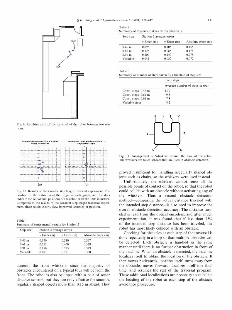
Fig. 9. Resulting path of the traversal of the robot between two sta-

tions.

Fig. 10. Results of the variable step length traversal experiment. The

position of the station is at the origin of each graph, and the dots

indicate the actual final positions of the robot, with the units in metres.

Compared to the results of the constant step length traversal experi-

ment, these results clearly slow improved accuracy of position.

Table 1

Summary of experimental results for Station 2

Step size Station 2 average errors

x Error (m) y Error (m) Absolute error (m)

0.46 m 0.150 0.310 0.367

0.61 m 0.215 0.460 0.529

0.91 m 0.180 0.295 0.379

Variable 0.087 0.281 0.300

Table 2

Summary of experimental results for Station 3

Step size Station 3 average errors

x Error (m) y Error (m) Absolute error (m)

0.46 m 0.095 0.105 0.155

0.61 m 0.125 0.085 0.178

0.91 m 0.200 0.140 0.278

Variable 0.041 0.052 0.072

Table 3

Summary of number of steps taken as a function of step size

Tour steps

Average number of steps in tour

Const. steps: 0.46 m 13.9



Variable steps 8.2

Fig. 11. Arrangement of �whiskers’ around the base of the robot.

The whiskers are touch sensors that are used in obstacle detection.


account the front whiskers, since the majority of

obstacles encountered on a typical tour will be from the

front. The robot is also equipped with a pair of sonar

distance sensors, but they are only effective for smooth,

regularly shaped objects more than 0.15 m ahead. They

proved insufficient for handling irregularly shaped ob-

jects such as chairs, so the whiskers were used instead.

Unfortunately, the whiskers cannot sense all the

possible points of contact on the robot, so that the robotcould collide with an obstacle without activating any of

the whiskers. Thus a second obstacle detection

method––comparing the actual distance traveled with

the intended step distance––is also used to improve the

overall obstacle detection accuracy. The distance trav-

eled is read from the optical encoders, and after much

experimentation, it was found that if less than 75%

of the intended step distance has been traveled, therobot has most likely collided with an obstacle.

Checking for obstacles at each step of the traversal is

done repeatedly in a loop so that multiple obstacles can

be detected. Each obstacle is handled in the same

manner until there is no further obstruction in front of

the machine. When an obstacle is detected, the machine

localizes itself to obtain the location of the obstacle. It

then moves backwards, localizes itself, turns away fromthe obstacle, moves forward, localizes itself one final

time, and resumes the rest of the traversal program.

These additional localizations are necessary to calculate

the heading of the robot at each step of the obstacle

avoidance procedure.


After the robot has moved away from the obstacle,the direction to turn, either left or right, is determined

based on the current heading direction and current

location of the robot. The aim is to turn such that

subsequent forward motion will tend to be toward the

center of the room, in order to avoid losing the robot off

the edges of the localization region. When the robot is

not near the edges, the direction of the turn depends on

the whiskers being pressed so that the robot turns away

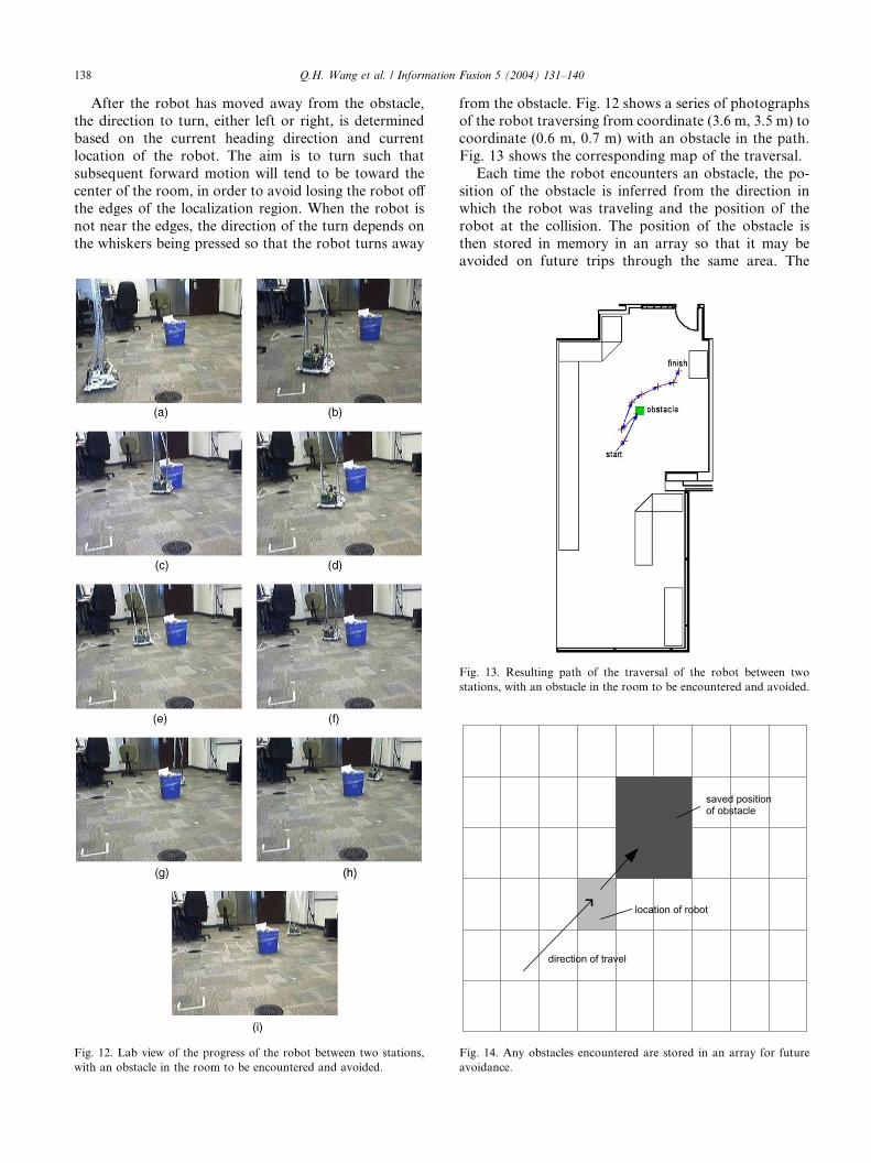
Fig. 12. Lab view of the progress of the robot between two stations,

with an obstacle in the room to be encountered and avoided.

from the obstacle. Fig. 12 shows a series of photographsof the robot traversing from coordinate (3.6 m, 3.5 m) to

coordinate (0.6 m, 0.7 m) with an obstacle in the path.

Fig. 13 shows the corresponding map of the traversal.

Each time the robot encounters an obstacle, the po-

sition of the obstacle is inferred from the direction in

which the robot was traveling and the position of the

robot at the collision. The position of the obstacle is

then stored in memory in an array so that it may beavoided on future trips through the same area. The

Fig. 13. Resulting path of the traversal of the robot between two

stations, with an obstacle in the room to be encountered and avoided.

direction of travel

location of robot

saved positionof obstacle

Fig. 14. Any obstacles encountered are stored in an array for future

avoidance.


relationship between the position of the robot at thecollision, the position of the saved obstacle, and the

direction of travel are shown in Fig. 14.

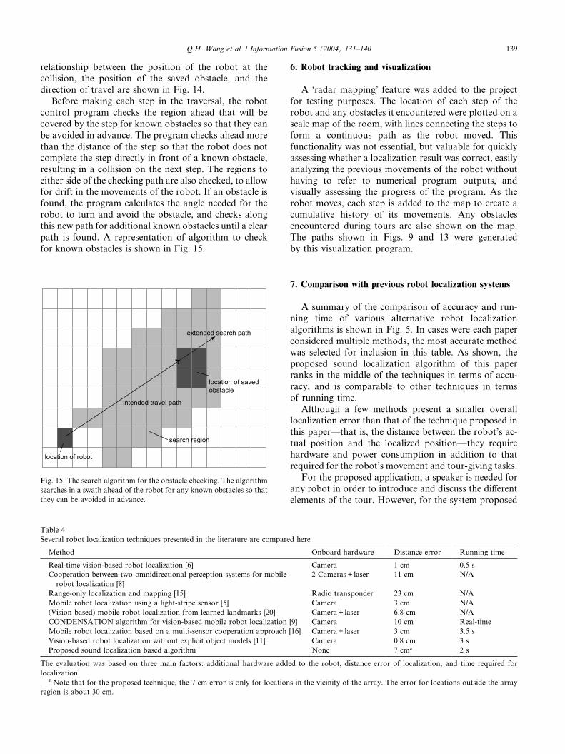
Before making each step in the traversal, the robot

control program checks the region ahead that will be

covered by the step for known obstacles so that they can

be avoided in advance. The program checks ahead more

than the distance of the step so that the robot does not

complete the step directly in front of a known obstacle,resulting in a collision on the next step. The regions to

either side of the checking path are also checked, to allow

for drift in the movements of the robot. If an obstacle is

found, the program calculates the angle needed for the

robot to turn and avoid the obstacle, and checks along

this new path for additional known obstacles until a clear

path is found. A representation of algorithm to check

for known obstacles is shown in Fig. 15.

location of robot

intended travel path

extended search path

search region

location of saved obstacle

Fig. 15. The search algorithm for the obstacle checking. The algorithm

searches in a swath ahead of the robot for any known obstacles so that

they can be avoided in advance.

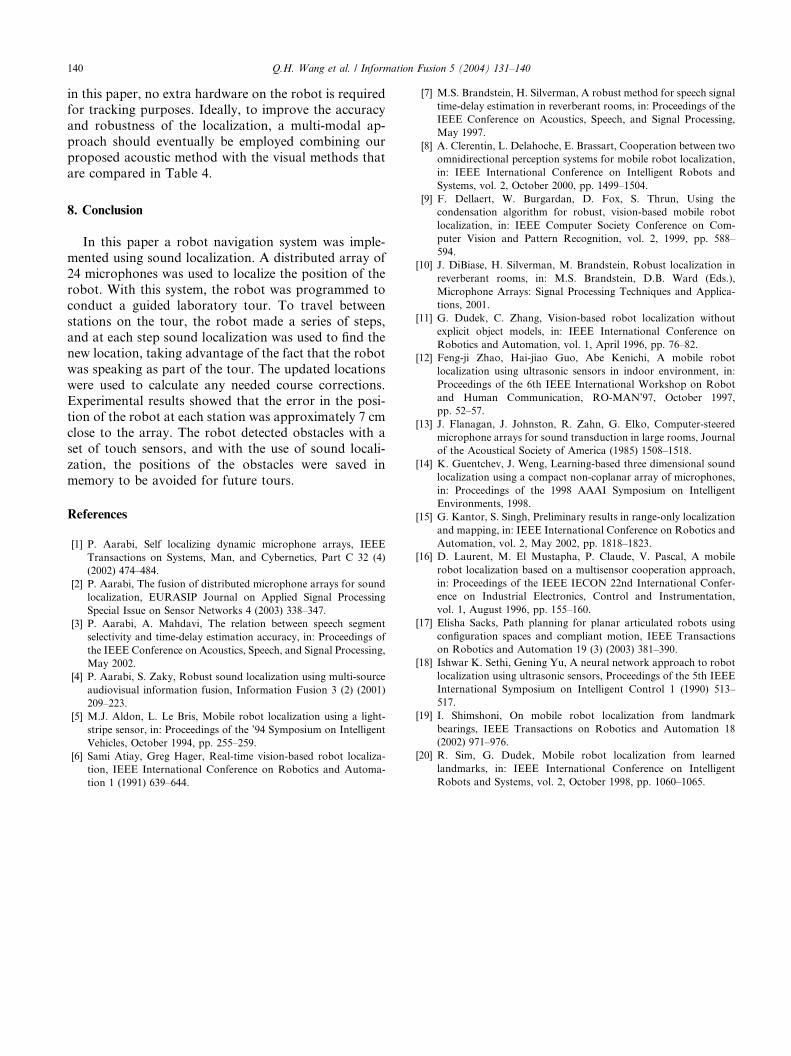
Table 4

Several robot localization techniques presented in the literature are compare

Method

Real-time vision-based robot localization [6]

Cooperation between two omnidirectional perception systems for mobile

robot localization [8]

Range-only localization and mapping [15]

Mobile robot localization using a light-stripe sensor [5]

(Vision-based) mobile robot localization from learned landmarks [20]

CONDENSATION algorithm for vision-based mobile robot localization

Mobile robot localization based on a multi-sensor cooperation approach

Vision-based robot localization without explicit object models [11]

Proposed sound localization based algorithm

The evaluation was based on three main factors: additional hardware add

localization.aNote that for the proposed technique, the 7 cm error is only for location

region is about 30 cm.

6. Robot tracking and visualization

A �radar mapping’ feature was added to the project

for testing purposes. The location of each step of the

robot and any obstacles it encountered were plotted on a

scale map of the room, with lines connecting the steps to

form a continuous path as the robot moved. This

functionality was not essential, but valuable for quickly

assessing whether a localization result was correct, easilyanalyzing the previous movements of the robot without

having to refer to numerical program outputs, and

visually assessing the progress of the program. As the

robot moves, each step is added to the map to create a

cumulative history of its movements. Any obstacles

encountered during tours are also shown on the map.

The paths shown in Figs. 9 and 13 were generated

by this visualization program.

7. Comparison with previous robot localization systems

A summary of the comparison of accuracy and run-

ning time of various alternative robot localization

algorithms is shown in Fig. 5. In cases were each paper

considered multiple methods, the most accurate method

was selected for inclusion in this table. As shown, the

proposed sound localization algorithm of this paperranks in the middle of the techniques in terms of accu-

racy, and is comparable to other techniques in terms

of running time.

Although a few methods present a smaller overall

localization error than that of the technique proposed in

this paper––that is, the distance between the robot’s ac-

tual position and the localized position––they require

hardware and power consumption in addition to thatrequired for the robot’s movement and tour-giving tasks.

For the proposed application, a speaker is needed for

any robot in order to introduce and discuss the different

elements of the tour. However, for the system proposed

d here

Onboard hardware Distance error Running time

Camera 1 cm 0.5 s

2 Cameras+ laser 11 cm N/A

Radio transponder 23 cm N/A

Camera 3 cm N/A

Camera+ laser 6.8 cm N/A

[9] Camera 10 cm Real-time

[16] Camera+ laser 3 cm 3.5 s

Camera 0.8 cm 3 s

None 7 cma 2 s

ed to the robot, distance error of localization, and time required for

s in the vicinity of the array. The error for locations outside the array


in this paper, no extra hardware on the robot is requiredfor tracking purposes. Ideally, to improve the accuracy

and robustness of the localization, a multi-modal ap-

proach should eventually be employed combining our

proposed acoustic method with the visual methods that

are compared in Table 4.

8. Conclusion

In this paper a robot navigation system was imple-

mented using sound localization. A distributed array of24 microphones was used to localize the position of the

robot. With this system, the robot was programmed to

conduct a guided laboratory tour. To travel between

stations on the tour, the robot made a series of steps,

and at each step sound localization was used to find the

new location, taking advantage of the fact that the robot

was speaking as part of the tour. The updated locations

were used to calculate any needed course corrections.Experimental results showed that the error in the posi-

tion of the robot at each station was approximately 7 cm

close to the array. The robot detected obstacles with a

set of touch sensors, and with the use of sound locali-

zation, the positions of the obstacles were saved in

memory to be avoided for future tours.

References

[1] P. Aarabi, Self localizing dynamic microphone arrays, IEEE

Transactions on Systems, Man, and Cybernetics, Part C 32 (4)

(2002) 474–484.

[2] P. Aarabi, The fusion of distributed microphone arrays for sound

localization, EURASIP Journal on Applied Signal Processing

Special Issue on Sensor Networks 4 (2003) 338–347.

[3] P. Aarabi, A. Mahdavi, The relation between speech segment

selectivity and time-delay estimation accuracy, in: Proceedings of

the IEEE Conference on Acoustics, Speech, and Signal Processing,

May 2002.

[4] P. Aarabi, S. Zaky, Robust sound localization using multi-source

audiovisual information fusion, Information Fusion 3 (2) (2001)

209–223.

[5] M.J. Aldon, L. Le Bris, Mobile robot localization using a light-

stripe sensor, in: Proceedings of the ’94 Symposium on Intelligent

Vehicles, October 1994, pp. 255–259.

[6] Sami Atiay, Greg Hager, Real-time vision-based robot localiza-

tion, IEEE International Conference on Robotics and Automa-

tion 1 (1991) 639–644.

[7] M.S. Brandstein, H. Silverman, A robust method for speech signal

time-delay estimation in reverberant rooms, in: Proceedings of the

IEEE Conference on Acoustics, Speech, and Signal Processing,

May 1997.

[8] A. Clerentin, L. Delahoche, E. Brassart, Cooperation between two

omnidirectional perception systems for mobile robot localization,

in: IEEE International Conference on Intelligent Robots and

Systems, vol. 2, October 2000, pp. 1499–1504.

[9] F. Dellaert, W. Burgardan, D. Fox, S. Thrun, Using the

condensation algorithm for robust, vision-based mobile robot

localization, in: IEEE Computer Society Conference on Com-

puter Vision and Pattern Recognition, vol. 2, 1999, pp. 588–

594.

[10] J. DiBiase, H. Silverman, M. Brandstein, Robust localization in

reverberant rooms, in: M.S. Brandstein, D.B. Ward (Eds.),

Microphone Arrays: Signal Processing Techniques and Applica-

tions, 2001.

[11] G. Dudek, C. Zhang, Vision-based robot localization without

explicit object models, in: IEEE International Conference on

Robotics and Automation, vol. 1, April 1996, pp. 76–82.

[12] Feng-ji Zhao, Hai-jiao Guo, Abe Kenichi, A mobile robot

localization using ultrasonic sensors in indoor environment, in:

Proceedings of the 6th IEEE International Workshop on Robot

and Human Communication, RO-MAN’97, October 1997,

pp. 52–57.

[13] J. Flanagan, J. Johnston, R. Zahn, G. Elko, Computer-steered

microphone arrays for sound transduction in large rooms, Journal

of the Acoustical Society of America (1985) 1508–1518.

[14] K. Guentchev, J. Weng, Learning-based three dimensional sound

localization using a compact non-coplanar array of microphones,

in: Proceedings of the 1998 AAAI Symposium on Intelligent

Environments, 1998.

[15] G. Kantor, S. Singh, Preliminary results in range-only localization

and mapping, in: IEEE International Conference on Robotics and

Automation, vol. 2, May 2002, pp. 1818–1823.

[16] D. Laurent, M. El Mustapha, P. Claude, V. Pascal, A mobile

robot localization based on a multisensor cooperation approach,

in: Proceedings of the IEEE IECON 22nd International Confer-

ence on Industrial Electronics, Control and Instrumentation,

vol. 1, August 1996, pp. 155–160.

[17] Elisha Sacks, Path planning for planar articulated robots using

configuration spaces and compliant motion, IEEE Transactions

on Robotics and Automation 19 (3) (2003) 381–390.

[18] Ishwar K. Sethi, Gening Yu, A neural network approach to robot

localization using ultrasonic sensors, Proceedings of the 5th IEEE

International Symposium on Intelligent Control 1 (1990) 513–

517.

[19] I. Shimshoni, On mobile robot localization from landmark

bearings, IEEE Transactions on Robotics and Automation 18

(2002) 971–976.

[20] R. Sim, G. Dudek, Mobile robot localization from learned

landmarks, in: IEEE International Conference on Intelligent

Robots and Systems, vol. 2, October 1998, pp. 1060–1065.

Documents

Acoustic robot navigation using distributed microphone arrays