Embed Size (px)
Citation preview
1. Introduction
Absorption or gas absorption is a unit operation used
in chemical industry and increasingly in environmental
applications. It a mass-transfer process in which a vapor
solute A in a gas mixture is absorbed by means of a liquid
in which the solute is more or less soluble. An example is
the absorption of the solute ammonia from air.
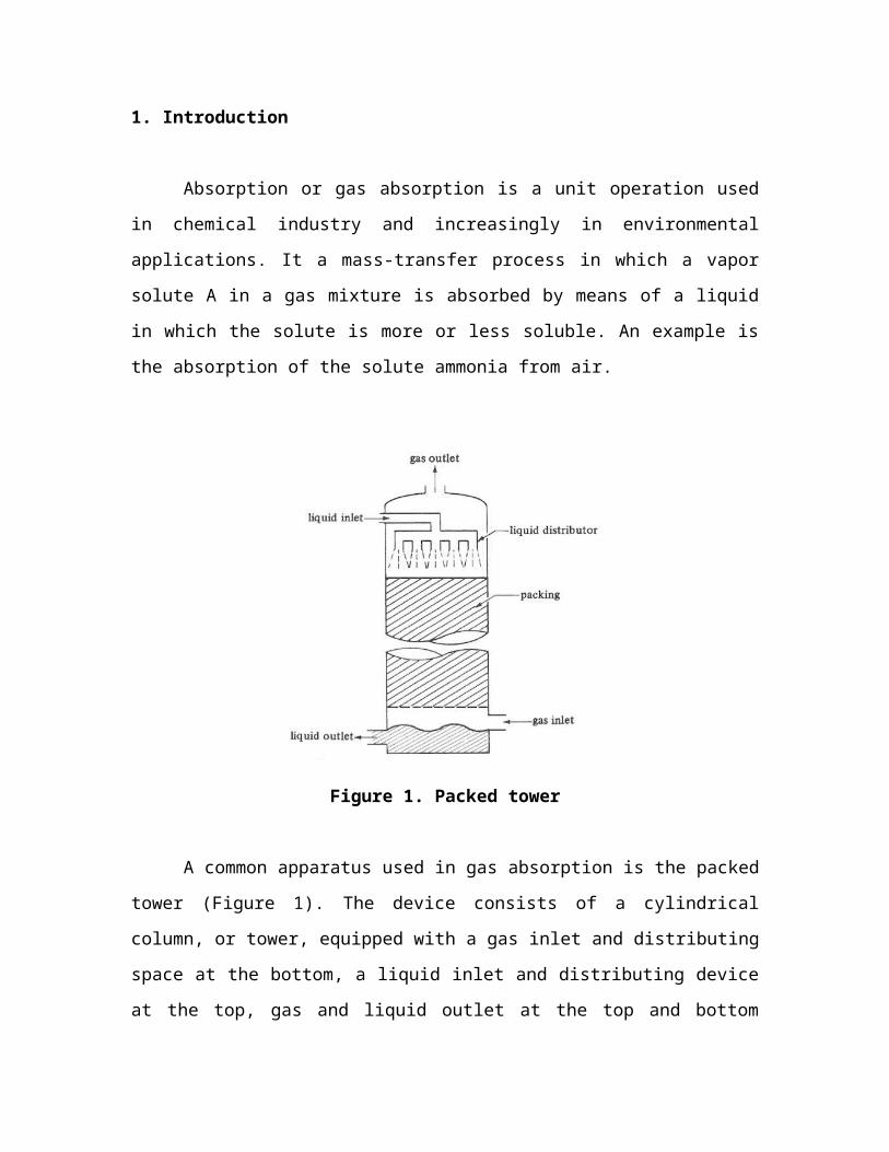
Figure 1. Packed tower
A common apparatus used in gas absorption is the packed
tower (Figure 1). The device consists of a cylindrical
column, or tower, equipped with a gas inlet and distributing
space at the bottom, a liquid inlet and distributing device
at the top, gas and liquid outlet at the top and bottom
respectively, and supported mass of inert solid shapes,
called packing. Packed columns are relatively simple devices
compared to plate columns. They can be categorized according
to the type of flow used in the operation: counter current,
co-current, and crosscurrent modes. The column used in this
experiment is operated in countercurrent flow, which is the
most frequently used type operation.
In a given packed tower with a given type and size of
packing and with definite flow of liquid, the upper limit to
the rate of gas flow is called the flooding velocity. The
tower cannot operate above this gas velocity. In a
countercurrent packed gas-liquid tower, the gas phase will
pass upward through the column. In order to let the gas
phase flow, there must be a sufficient pressure drop to
overcome the friction and form drag caused by the packing
and the falling liquid. The liquid must fall down against
this pressure drop by means of gravitational force. Once the
liquid is distributed over the top of the packing, the
liquid ideally flows in thin films over the entire packing
surface, but what really happens is the films tend to grow
thicker in some places and thinner in others, so that the
liquid collects into small rivulets and flows along
localized paths through the packing, especially at low
liquid rates. This is known as channeling. Loading point is
the point where the liquid will start to accumulate in the
column and when the gas flow increases further, flooding
point is reached. It is the point when the liquid in the
column will overflow.
2. Objectives of the experiment
Determine experimentally the pressured drop across a
wet packed column as a function of the air flow rate
and compare the results with theoretically calculated
values
Determine through visual observation and by graphical
methods the loading and flooding points of the packed
column at preset values of water flow rates
Construct form experimental data the loading and
flooding curves of the packed column based on the
generalized correlations proposed by Sherwood, Shipley
and Holloway
3. Methodology
3.1 Materials
Water
3.2 Equipment and Apparatus
Packed Absorption Column (with Raschig ring random
packing)
Stopwatch
Thermometer
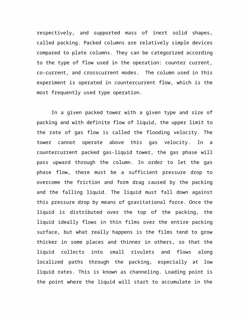
Figure 1. Packed Absorption Column
Parts of a Packed Absorption Column
(1) Sump tank
(2) Valve in the discharge pipe to the sump tank
(3) Water(left) and mercury(right) manometers
(4) Air Flow meter
(5) Gas analyzing equipment
(6) Air flow valve
(7) Upper stopcock (S2)
(8) Water flow valve
(9) Air flow meter
(10) CO2flow meter
(11) Lower Stop cock (S3)
(12) Air pump
(13) Water pump
(14) Down-coming tube
3.3 Procedures
3.3-1. Preliminary Preparations
The valve in the water discharge tube was opened while
the drains under the tank and down-coming tube were closed.
The tank was filled with distilled water up to three fourth
its volume. The three 3-way cocks between the column and
manometer were positioned in such a way that only the water
manometer is used to measure the pressure drop.
3.3-2. Pressure Drop in a Wetted Column
In this part of the experiment, the pressure drop in a
wetted column was determined using conditions number two (2)
from Table 422-5.1 of the manual. The gas and water flow
meters and the stopcocks were closed, while C4 was fully
opened. The water pump was switched on and the flow rate was
set to 3-4 liters/minutes. The pump ran for two to three
minutes before the pump was turned off. The column was
drained for five minutes. With S2 and S3 open, manometer
readings of pressure differences across the column were
taken for airflow rates ranging from 20 to 170 liters/minute
starting with low rates. Another trial was done but this
time starting with the highest flow rate which is from 170
down to 20 liters/minute. At least ten flow rates were
tested for each trial. The operational temperatures of the
liquid and the gas were recorded at the start and end of the
experiment. The pressure drop across the wet column were
calculated from using the manometer readings obtained. These
experimental values were plotted against air flow rates and
were compared with theoretical values.
3.3-3. Identifying the Loading and Flooding Points
In this part of the experiment the loading and flooding
points of the packed column were identified using conditions
number two (2) for Part C from Table 422-5.1 of the manual.
The operational temperatures of the liquid and the gas were
recorded at the start and end of this experiment. For each
assigned value of water flow rate, ten air flow rates were
applied ranging from 20 to 170 liters/minute. Visual
observations of the column at each setting were noted and
through this the loading and flooding points of the column
were identified. The loading point is the point when water
started to accumulate the column while the flooding point is
the point when the water level has reached the top of the
packing in the column. Manometer readings of pressure
difference across the column were recorded per air flow
rate. Pressure drop was calculated and plotted against gas
mass velocity to determine the loading and flooding points
graphically. Using experimental data the loading and
flooding curves of the packed column were constructed based
on the generalized correlations proposed by Sherwood,
Shipley and Holloway.
3.3-4. Shut Down Operations
After the experiment, the water tank and the water from
the down-coming tube were drained and then their valves were
closed.
4. Results and Discussions
4.1 Pressure Drop in a Wetted Column
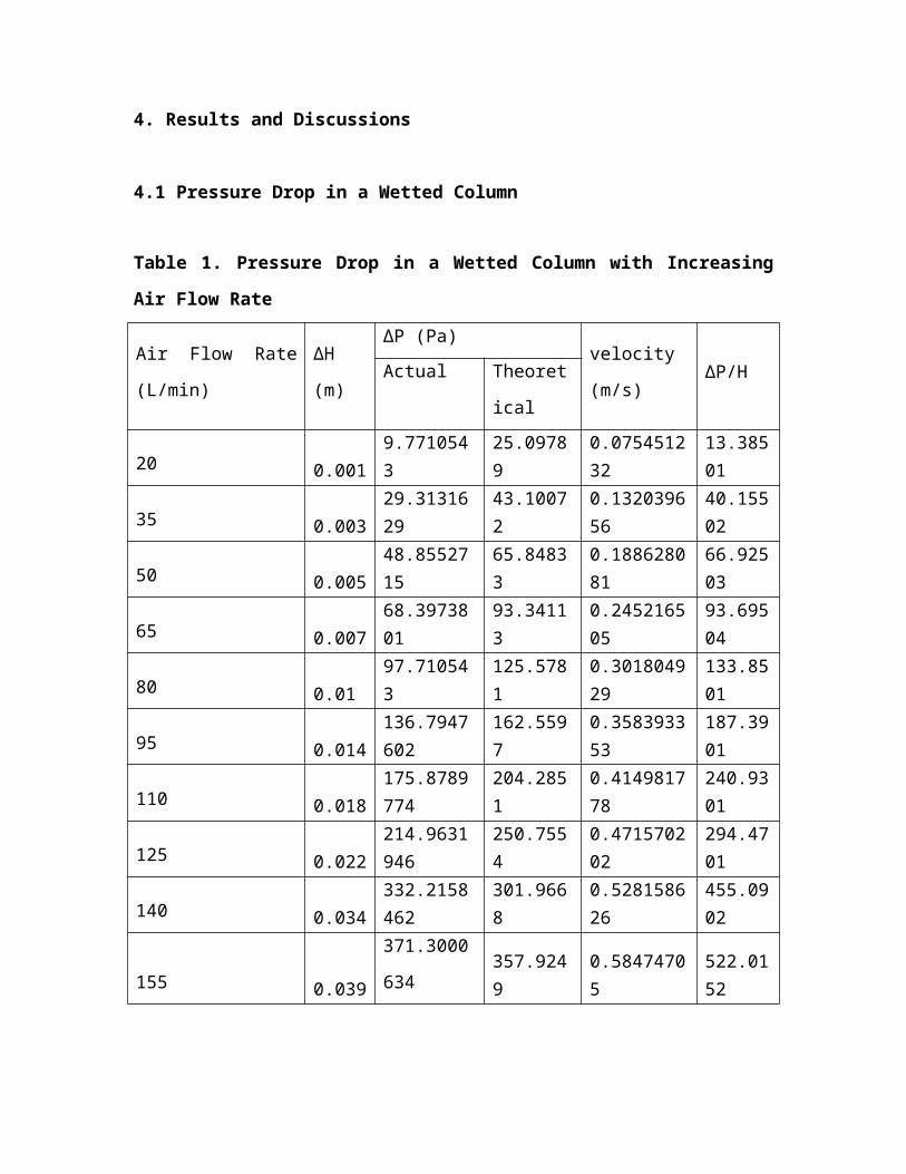
Table 1. Pressure Drop in a Wetted Column with Increasing
Air Flow Rate
Air Flow Rate
(L/min)
∆H
(m)
∆P (Pa)velocity
(m/s)∆P/HActual Theoret
ical
20 0.0019.7710543
25.09789
0.075451232
13.38501
35 0.00329.3131629
43.10072
0.132039656
40.15502
50 0.00548.8552715
65.84833
0.188628081
66.92503
65 0.00768.3973801
93.34113
0.245216505
93.69504
80 0.0197.710543
125.5781
0.301804929
133.8501
95 0.014136.7947602
162.5597
0.358393353
187.3901
110 0.018175.8789774
204.2851
0.414981778
240.9301
125 0.022214.9631946
250.7554
0.471570202
294.4701
140 0.034332.2158462
301.9668
0.528158626
455.0902
155 0.039
371.3000
634357.9249
0.58474705
522.0152
170 0.044
390.8421
72418.6293
0.641335474
588.9403
* Twater = 29°C, Tair = 26°C
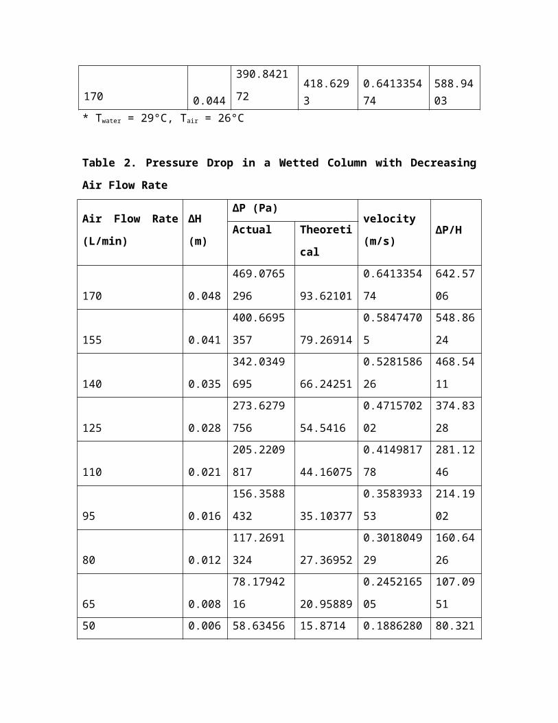
Table 2. Pressure Drop in a Wetted Column with Decreasing
Air Flow Rate
Air Flow Rate
(L/min)
∆H
(m)
∆P (Pa)velocity
(m/s)∆P/HActual Theoreti
cal
170 0.048
469.0765
296 93.62101
0.6413354
74
642.57
06
155 0.041
400.6695
357 79.26914
0.5847470
5
548.86
24
140 0.035
342.0349
695 66.24251
0.5281586
26
468.54
11
125 0.028
273.6279
756 54.5416
0.4715702
02
374.83
28
110 0.021
205.2209
817 44.16075
0.4149817
78
281.12
46
95 0.016
156.3588
432 35.10377
0.3583933
53
214.19
02
80 0.012
117.2691
324 27.36952
0.3018049
29
160.64
26
65 0.008
78.17942
16 20.95889
0.2452165
05
107.09
5150 0.006 58.63456 15.8714 0.1886280 80.321
62 81 32
35 0.003
29.31728
31 12.10808
0.1320396
56
40.160
66
20 0.003
29.31728
31 9.668494
0.0754512
32
40.160
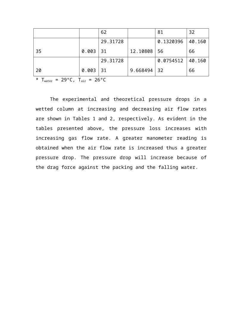
66* Twater = 29°C, Tair = 26°C
The experimental and theoretical pressure drops in a
wetted column at increasing and decreasing air flow rates
are shown in Tables 1 and 2, respectively. As evident in the
tables presented above, the pressure loss increases with
increasing gas flow rate. A greater manometer reading is
obtained when the air flow rate is increased thus a greater
pressure drop. The pressure drop will increase because of
the drag force against the packing and the falling water.
0 0.1 0.2 0.3 0.4 0.5 0.6 0.7 0.80
100
200
300
400
500
600
700
Air Flow Rates
Theoretical Pressure DropDecreasing Air Flow RateIncreasing Air Flow RateDry Column
v (m/s)
∆P/H
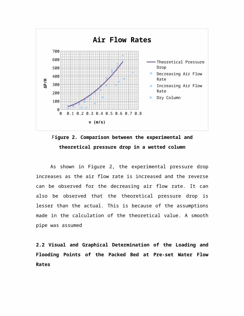
Figure 2. Comparison between the experimental and
theoretical pressure drop in a wetted column
As shown in Figure 2, the experimental pressure drop
increases as the air flow rate is increased and the reverse
can be observed for the decreasing air flow rate. It can
also be observed that the theoretical pressure drop is
lesser than the actual. This is because of the assumptions
made in the calculation of the theoretical value. A smooth
pipe was assumed
2.2 Visual and Graphical Determination of the Loading and
Flooding Points of the Packed Bed at Pre-set Water Flow
Rates
Flooding and loading points were determined both
graphically and through visual observation. Loading point
was observed when the water started to accumulate at the
base of the column whereas the flooding point was observed
when the water level reached the topmost part of the packing
in the column.
The loading and flooding point was determined
graphically by plotting log (∆P/∆L) against log vo which is
shown in figure 3. The points where there is a drastic
change in the slope of the curve are the loading and
flooding points.
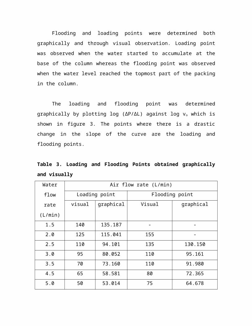
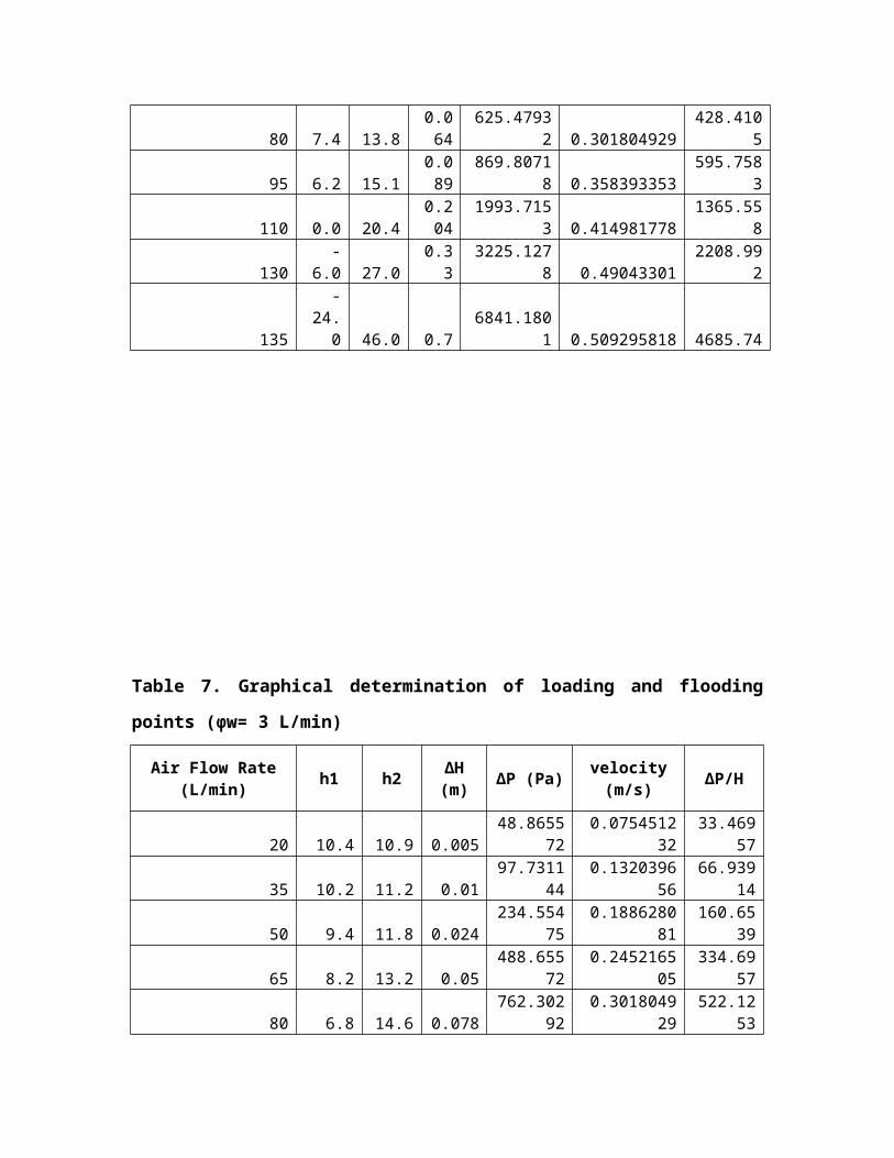
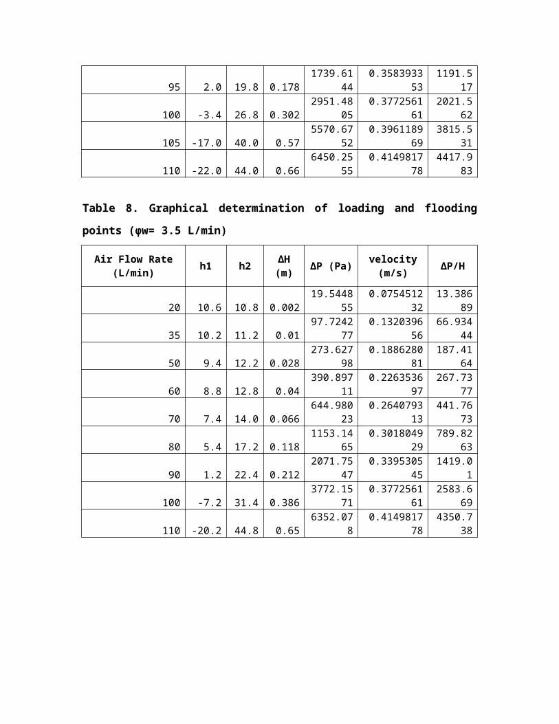
Table 3. Loading and Flooding Points obtained graphically
and visually
Water
flow
rate
(L/min)
Air flow rate (L/min)Loading point Flooding point
visual graphical Visual graphical
1.5 140 135.187 - -2.0 125 115.041 155 -2.5 110 94.101 135 130.1503.0 95 80.052 110 95.1613.5 70 73.160 110 91.9804.5 65 58.581 80 72.3655.0 50 53.014 75 64.678
Based on the table above, it is observed that as the
liquid water flow rate is increased, the air flow rates at
which loading and flooding are observed decrease. This
occurs because the higher the water flow rate, the easier it
is for the liquid to accumulate due to the significant
decrease in the area of path of the gas to flow. The area is
decreased by the resisting liquid flow countercurrent to the
flow of gas.
For the graphical method, the flooding point was not
reached for water flow rates 1.5 L/min and 2.0 L/min because
it was observed that the height of the water almost reached
the topmost part of the column therefore no further readings
were made.
2.2Loading and Flooding Curves of the Packed Column From
Experimental Data Based on the Generalized Correlations
Proposed by Sherwood, Shipley and Holloway
Empirical correlations for various random packing based
on experimental data are used to predict the pressure drop
in the gas flow. Sherwood, Shipley and Holloway proposed the
first generalized correlation for flooding of packed columns
based on tests done with air-water systems.
0.3 3
0.005
Loading Based on Visual Observation
Power (Loading Based on Visual Observation)
Flooding Based on Visual Observation
Power (Flooding Based on Visual Observation)
Loading Based on Graphical Method
Power (Loading Based on Graphical Method)
Flooding Based on Graphical Method
Power (Flooding Based on Graphical Method)
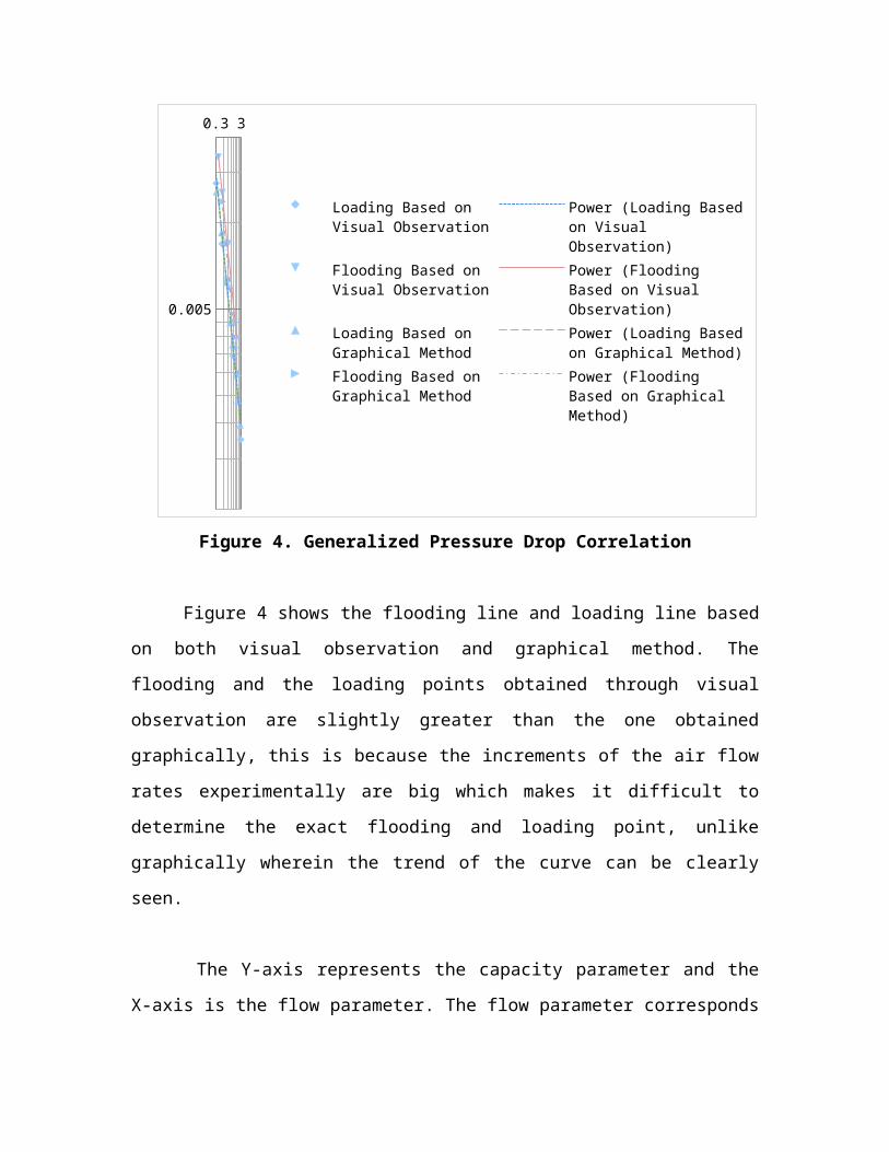
Figure 4. Generalized Pressure Drop Correlation
Figure 4 shows the flooding line and loading line based
on both visual observation and graphical method. The
flooding and the loading points obtained through visual
observation are slightly greater than the one obtained
graphically, this is because the increments of the air flow
rates experimentally are big which makes it difficult to
determine the exact flooding and loading point, unlike
graphically wherein the trend of the curve can be clearly
seen.
The Y-axis represents the capacity parameter and the
X-axis is the flow parameter. The flow parameter corresponds
to the liquid-to-gas kinetic energy ratio while the capacity
parameter is a function of the square of the actual gas
velocity [Seader, 2006]. The figure above shows that the
capacity parameter decreases with increasing flow parameter.
This is because an increase in water flow rate increases the
liquid-to-gas kinetic energy. A decrease in this ratio
causes a decrease in the capacity parameter.
5. Conclusion
Absorption is a unit operation that contacts two phases
—usually a gas and a liquid—where the more gas soluble
solute is absorbed from the liquid. To increase contact
between the two and increase efficiency as a consequence,
packed beds are used. The presence of the packed beds
requires greater pressure for the gas to flow past it and
this result in pressure loss. As the air flow rate is
increased, the resulting pressure drops increase as well.
This is in agreement with the results if the pressure losses
are to be calculated theoretically. The use of Erguns
equation for the pressure drop in a packed bed, as well as
Hagen-Poisuille equation to account for the parts of the
absorption column free of the packings, gives an increasing
pressure loss with increasing air flow rates.
One major problem that has to be given attention when
it comes to absorption is that of flooding. Flooding is the
point at which the liquid overflows the column as a result
of a high air flow rate. The prelude to this point is the
loading point which can be observed as the start of
accumulation of the liquid in the packings. Aside from these
visual observations, the flooding and loading points can be
determined using the graphical method as well. These help in
the designing of the absorption tower as most equipment run
on 50-70% only of the flooding velocity; that is why it is
important to know these two velocities.
Sherwood, Shipley and Holloway were some of the first
people that proposed a generalized correlation for flooding
and loading of packed columns. They plotted the ratio of the
kinetic energy of the gas to the potential energy in the
liquid versus the flow parameter—a dimensionless number that
measures the relative kinetic energy of the system. This
gives a downward slope curve resulting from tests using a
broad range of air and water velocities. In the experiment,
only a part of this curve was achieved.
6. References
Geankoplis, C.J. (2009). Transport Processes and Unit
Operations.4th Edition.
Prentice Hall,New Jersey.
Henley, E.J., Seader, J.D. (2006).Separation Process
Principles.2nd Edition. John
Wiley & Sons., New Jersey.
McCabe,W.L. et.al. (2001). Unit Operations of Chemical
Engineering.6th Edition,
McGraw-Hill., New York.
VII. Appendices
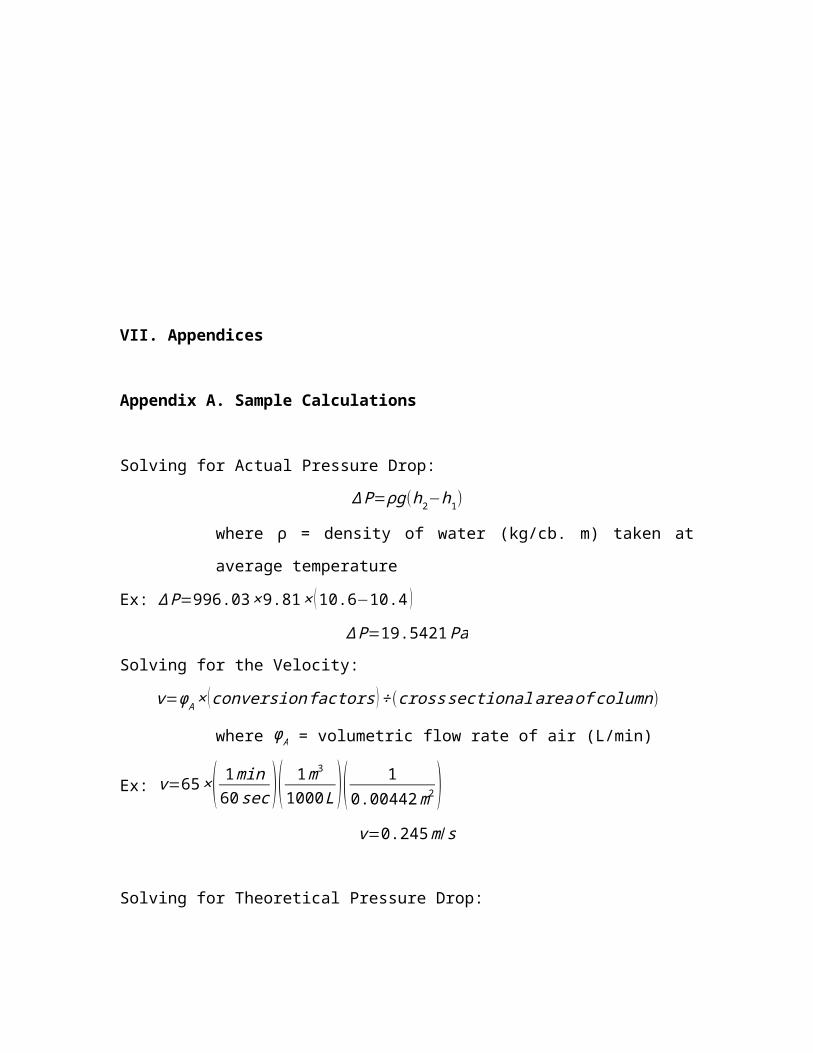
Appendix A. Sample Calculations
Solving for Actual Pressure Drop:
ΔP=ρg(h2−h1)
where ρ = density of water (kg/cb. m) taken at
average temperature
Ex: ΔP=996.03×9.81× (10.6−10.4 )
ΔP=19.5421PaSolving for the Velocity:
v=ϕA× (conversionfactors )÷(crosssectionalareaofcolumn)
where ϕA = volumetric flow rate of air (L/min)
Ex: v=65×( 1min60sec )( 1m3
1000L )( 10.00442m2 )v=0.245m/s
Solving for Theoretical Pressure Drop:
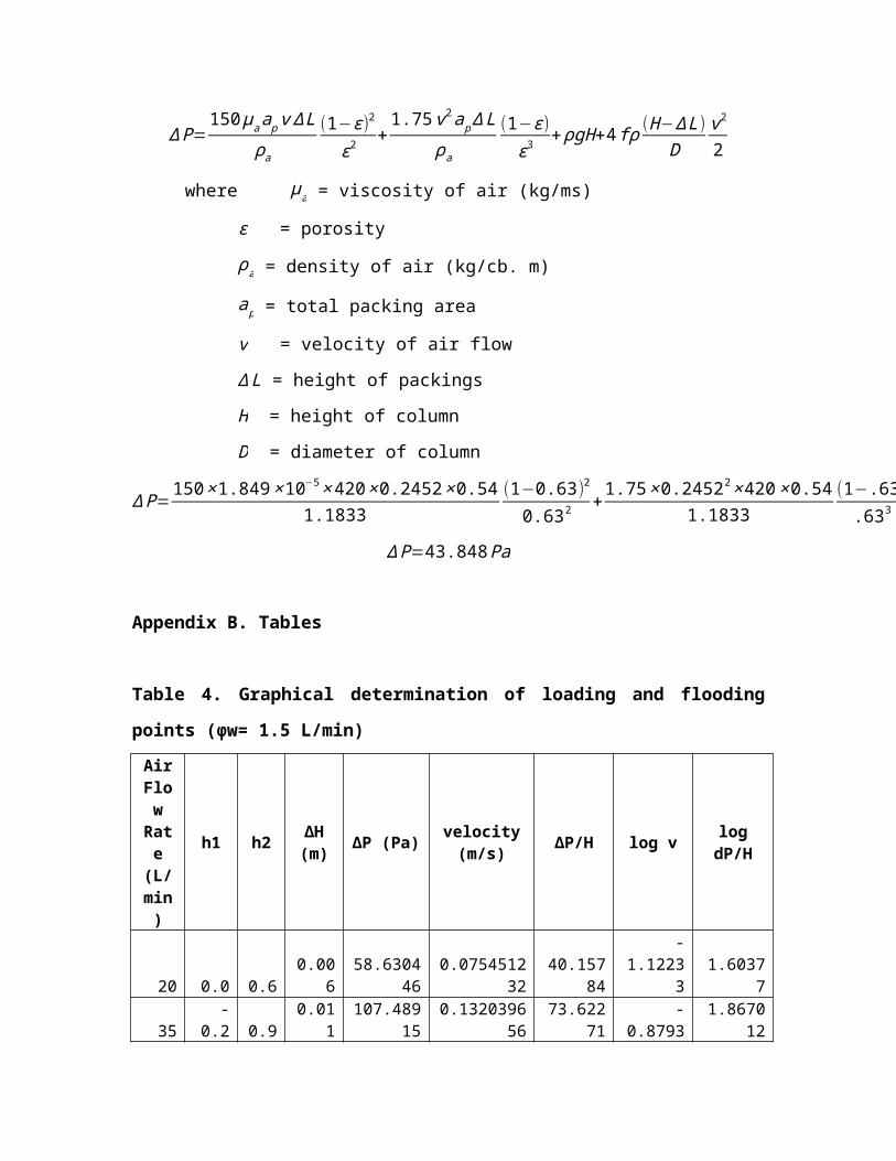
ΔP=150μaapv∆L
ρa(1−ε)2
ε2+1.75v2ap∆L
ρa
(1−ε)
ε3+ρgH+4fρ (H−∆L)
Dv2
2
where μa = viscosity of air (kg/ms)
ε = porosityρa = density of air (kg/cb. m)
ap = total packing area
v = velocity of air flow∆L = height of packingsH = height of columnD = diameter of column
ΔP=150×1.849×10−5×420×0.2452×0.54
1.1833(1−0.63)2
0.632 +1.75×0.24522×420×0.54
1.1833(1−.63)
.633 +1.1833×9.81×0.73+4×0.0142×1.1833 (0.73−0.54)0.075
0.24522
2
ΔP=43.848Pa
Appendix B. Tables
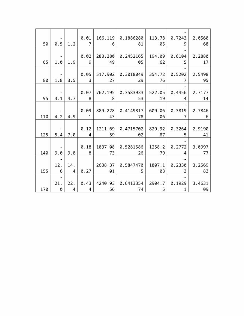
Table 4. Graphical determination of loading and flooding
points (φw= 1.5 L/min)AirFlowRate(L/min)
h1 h2 ∆H(m) ∆P (Pa) velocity
(m/s) ∆P/H log v logdP/H
20 0.0 0.60.00
658.6304
460.0754512
3240.157
84
-1.1223
31.6037
7
35-
0.2 0.90.01
1107.489
150.1320396
5673.622
71-
0.87931.8670
12
50-
0.5 1.20.01
7166.119
60.1886280
81113.78
05
-0.7243
92.0560
68
65-
1.0 1.90.02
9283.380
490.2452165
05194.09
62
-0.6104
52.2880
17
80-
1.8 3.50.05
3517.902
270.3018049
29354.72
76
-0.5202
72.5498
95
95-
3.1 4.70.07
8762.195
80.3583933
53522.05
19
-0.4456
42.7177
14
110-
4.2 4.90.09
1889.228
430.4149817
78609.06
06
-0.3819
72.7846
6
125-
5.4 7.00.12
41211.69
590.4715702
02829.92
87
-0.3264
52.9190
41
140-
9.0 9.80.18
81837.08
730.5281586
261258.2
79
-0.2772
43.0997
77
155
-12.
614.4 0.27
2638.3701
0.58474705
1807.103
-0.2330
33.2569
83
170
-21.
022.4
0.434
4240.9356
0.641335474
2904.75
-0.1929
13.4631
09
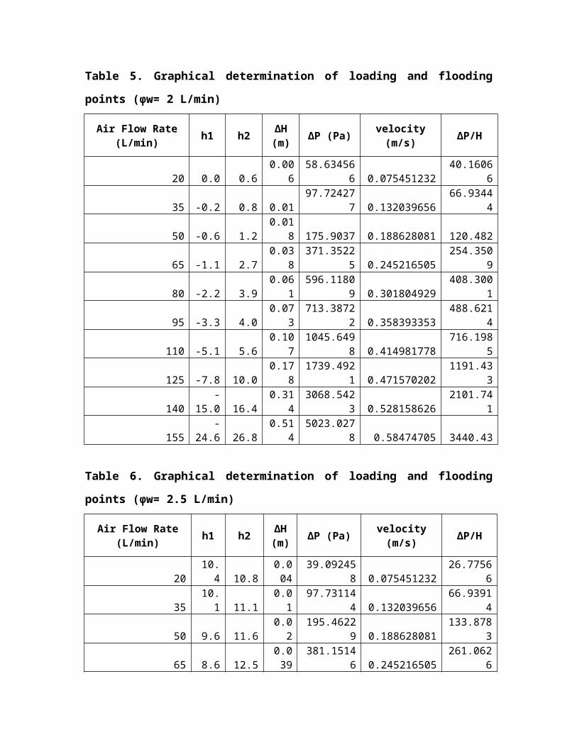
Table 5. Graphical determination of loading and flooding
points (φw= 2 L/min)
Air Flow Rate(L/min) h1 h2 ∆H
(m) ∆P (Pa) velocity(m/s) ∆P/H
20 0.0 0.60.00
658.63456
6 0.07545123240.1606
6
35 -0.2 0.8 0.0197.72427
7 0.13203965666.9344
4
50 -0.6 1.20.01
8 175.9037 0.188628081 120.482
65 -1.1 2.70.03
8371.3522
5 0.245216505254.350
9
80 -2.2 3.90.06
1596.1180
9 0.301804929408.300
1
95 -3.3 4.00.07
3713.3872
2 0.358393353488.621
4
110 -5.1 5.60.10
71045.649
8 0.414981778716.198
5
125 -7.8 10.00.17
81739.492
1 0.4715702021191.43
3
140-
15.0 16.40.31
43068.542
3 0.5281586262101.74
1
155-
24.6 26.80.51
45023.027
8 0.58474705 3440.43
Table 6. Graphical determination of loading and flooding
points (φw= 2.5 L/min)
Air Flow Rate(L/min) h1 h2 ∆H
(m) ∆P (Pa) velocity(m/s) ∆P/H
2010.
4 10.80.004
39.092458 0.075451232
26.77566
3510.
1 11.10.0
197.73114
4 0.13203965666.9391
4
50 9.6 11.60.0
2195.4622
9 0.188628081133.878
3
65 8.6 12.50.039
381.15146 0.245216505
261.0626
80 7.4 13.80.064
625.47932 0.301804929
428.4105
95 6.2 15.10.089
869.80718 0.358393353
595.7583
110 0.0 20.40.204
1993.7153 0.414981778
1365.558
130-
6.0 27.00.3
33225.127
8 0.490433012208.99
2
135
-24.
0 46.0 0.76841.180
1 0.509295818 4685.74
Table 7. Graphical determination of loading and flooding
points (φw= 3 L/min)
Air Flow Rate(L/min) h1 h2 ∆H
(m) ∆P (Pa) velocity(m/s) ∆P/H
20 10.4 10.9 0.00548.8655
720.0754512
3233.469
57
35 10.2 11.2 0.0197.7311
440.1320396
5666.939
14
50 9.4 11.8 0.024234.554
750.1886280
81160.65
39
65 8.2 13.2 0.05488.655
720.2452165
05334.69
57
80 6.8 14.6 0.078762.302
920.3018049
29522.12
53
95 2.0 19.8 0.1781739.61
440.3583933
531191.5
17
100 -3.4 26.8 0.3022951.48
050.3772561
612021.5
62
105 -17.0 40.0 0.575570.67
520.3961189
693815.5
31
110 -22.0 44.0 0.666450.25
550.4149817
784417.9
83
Table 8. Graphical determination of loading and flooding
points (φw= 3.5 L/min)
Air Flow Rate(L/min) h1 h2 ∆H
(m) ∆P (Pa) velocity(m/s) ∆P/H
20 10.6 10.8 0.00219.5448
550.0754512
3213.386
89
35 10.2 11.2 0.0197.7242
770.1320396
5666.934
44
50 9.4 12.2 0.028273.627
980.1886280
81187.41
64
60 8.8 12.8 0.04390.897
110.2263536
97267.73
77
70 7.4 14.0 0.066644.980
230.2640793
13441.76
73
80 5.4 17.2 0.1181153.14
650.3018049
29789.82
63
90 1.2 22.4 0.2122071.75
470.3395305
451419.0
1
100 -7.2 31.4 0.3863772.15
710.3772561
612583.6
69
110 -20.2 44.8 0.656352.07
80.4149817
784350.7
38
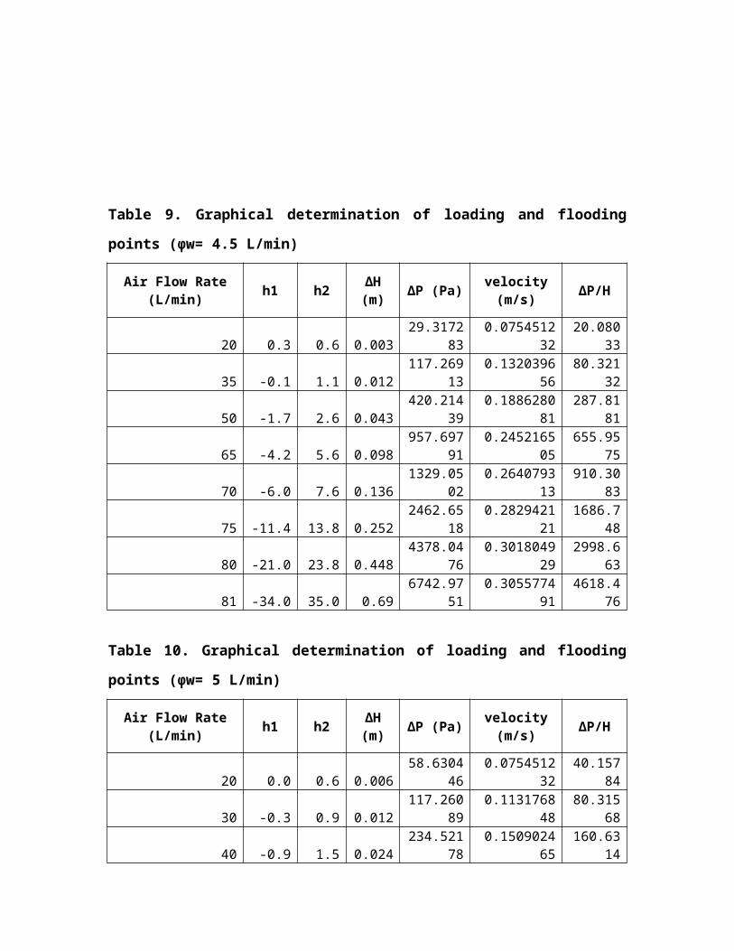
Table 9. Graphical determination of loading and flooding
points (φw= 4.5 L/min)
Air Flow Rate(L/min) h1 h2 ∆H
(m) ∆P (Pa) velocity(m/s) ∆P/H
20 0.3 0.6 0.00329.3172
830.0754512
3220.080
33
35 -0.1 1.1 0.012117.269
130.1320396
5680.321
32
50 -1.7 2.6 0.043420.214
390.1886280
81287.81
81
65 -4.2 5.6 0.098957.697
910.2452165
05655.95
75
70 -6.0 7.6 0.1361329.05
020.2640793
13910.30
83
75 -11.4 13.8 0.2522462.65
180.2829421
211686.7
48
80 -21.0 23.8 0.4484378.04
760.3018049
292998.6
63
81 -34.0 35.0 0.696742.97
510.3055774
914618.4
76
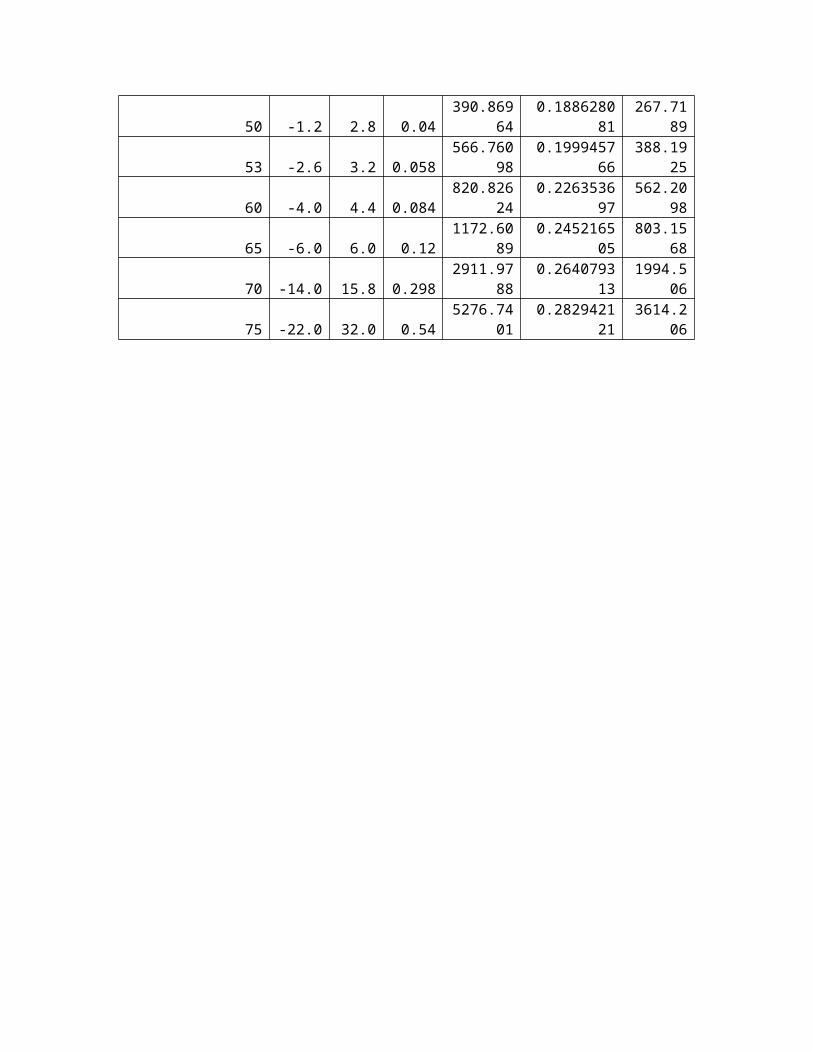
Table 10. Graphical determination of loading and flooding
points (φw= 5 L/min)
Air Flow Rate(L/min) h1 h2 ∆H
(m) ∆P (Pa) velocity(m/s) ∆P/H
20 0.0 0.6 0.00658.6304
460.0754512
3240.157
84
30 -0.3 0.9 0.012117.260
890.1131768
4880.315
68
40 -0.9 1.5 0.024234.521
780.1509024
65160.63
14
50 -1.2 2.8 0.04390.869
640.1886280
81267.71
89
53 -2.6 3.2 0.058566.760
980.1999457
66388.19
25
60 -4.0 4.4 0.084820.826
240.2263536
97562.20
98
65 -6.0 6.0 0.121172.60
890.2452165
05803.15
68
70 -14.0 15.8 0.2982911.97
880.2640793
131994.5
06
75 -22.0 32.0 0.545276.74
010.2829421
213614.2
06


