A Versatile Bistatic & Polarimetric Marine Radar Simulator

Andreas Arnold-Bos, Arnaud Martin, Ali Khenchaf

Laboratoire E3I2 (EA 3876)

Ecole Nationale Superieure des Ingenieurs des Etudes et Techniques de l’Armement (ENSIETA)

Brest, France

{arnoldan, martinar, khenchal}@ensieta.fr

Abstract: We present a versatile simulator for marine radars

that can, in particular, be used in multistatic configurations.

Today, most simulators modelize the sea clutter by a random

noise; however no obvious relation exists between physical

parameters (e.g. wind speed or salinity) and the shape of the

probabilistic law of noise. On the contrary, we modelize the

whole acquisition chain: antennas and their polarization, the

shape of the emitted signal, etc. Realistic sea surfaces are

generated using the two-scales model on a semi-deterministic

basis, so as to be able to incorporate the presence of ship

wakes. We present pseudo-raw signals obtained with our

simulator. These signals can be further processed and fed

to a ship detection and tracking chain. We aim at using

this simulation as a tool to benchmark these algorithms

and improve them by adding knowledge on the physical

uncertainties and the sensor imprecisions.

Keywords: Marine surveillance systems, bistatic radar,

bistatic scattering, radar simulation.

I. INTRODUCTION

On an average day, more than a hundred and fifty ships

transit through the English Channel. Among them, about eight

ships carry dangerous goods and could potentially be respon-

sible for ecological disasters similar as the sinking of Amoco

Cadiz (1978) or more recently, Erika (1999) and Prestige

(2002). Drug smuggling, illegal immigration, or piracy are

yet other rampant problems that marine authorities have to

face. To improve safety along coasts, especially in zones where

intense ship traffic occurs, detection and tracking algorithms

for radar-based surveillance systems must be continuously

improved. Doing so requires an important insight in the

physical phenomena that occur during the acquisition of the

data. The problem is that real data with extensive ground

truth are barely available today, especially with uncommon,

yet promising, configurations such as bistatic radar.

In this paper, we present a simulation tool for marine radars

that can be used in multistatic configurations and in various

working situations: real aperture or synthetic aperture radars,

shore-based or airborne radar. This simulator is intended to

help the benchmark of current or future ship detection and

tracking algorithms. Today, most radar simulators model the

sea clutter by a random noise, such as the Rayleigh or the

K-compound law [1]. Knowing that the signal coming from

the sea can be modeled as a known noise is a divine gift,

because it justifies the use of the much-celebrated Constant

False Alarm Rate (CFAR) schemes to distinguish ships from

waves when thresholding the return signal [2]. However no

obvious relation exists between physical parameters (e.g. wind

speed, salinity, etc) and the shape of the probabilistic law of

noise. Also, the influence of uncertainties on the motion of

the radar vector is seldom modeled. Finally, to the best of

our knowledge, all the simulators on the market are designed

for monostatic configurations where the transceiver and the

transmitter are the same.

To go past these shortcomings, we on the contrary opted to

model the whole acquisition chain. We consider among other

things the antennas and their polarization, the shape and the

frequency of the emitted signal, the influence of the weather on

the sea, etc. To determine the sea clutter, realistic sea surfaces

are generated using a two-scales model on a semi-deterministic

basis. On the largest scale, gravity waves are obtained by

synthesizing a random sea according to usual height spectra.

Using a ray-tracing technique, the local incidence angles

can be determined. Then, the scattering coefficients due to

smaller waves (capillary waves), are obtained using a statistical

description of the sea on small scales [3]. These coefficients

account for the diffusion of the electromagnetic wave due

to the roughness of the sea surface. This mixed approach

between determinism and statistical description, introduced by

[4], allows the user to incorporate the presence of ship wakes

on the deterministic part of the sea. Simulating ship wakes is

essential as it is a prominent feature in SAR images [5]. The

signature of the ship itself could be added by using a database

of radar cross sections (RCS) for various typical ships acquired

in our anechoic chamber.

Our paper is structured as follows. In section II, we present

the simulated bistatic configuration and the bistatic radar

equation which is the basis of our simulation. In section III, the

physical model of the sea is explained, and three approximate

methods are reviewed to compute the scattering matrix from

the model of the sea. Section IV explains the main steps of the

simulation algorithm. Finally, some first results are presented

and commented in the last section.

II. SIMULATED CONFIGURATION

The simulated configuration is presented in Fig. 1. It

consists of a transmitter X and a receiver R, placed at the

Fig. 1. Simulated configuration. The red arrows indicate the dependencies(some of them are omitted for the sake of brevity). (1): partially simulated;(2) not simulated.

same spatial position (monostatic configuration) or separated

(bistatic configuration). The antennas can either belong to

a coastal radar, an airborne radar, or a spaceborne radar.

Indeed, those will only be a specialization of the more generic

radar system that we model here. Such specialization can be

achieved either by i) tuning variables such as the antenna

shape, the carrier frequency or the transmitted signal shape,

ii) moving the antennas as if they were carried aboard a plane

or a satellite and iii) using specific post-processing algorithms,

such as (eventually bistatic) Synthetic Aperture reconstruction.

The target is the sea, which characteristics vary with the

wind speed, the salinity, the temperature, and the presence

(or absence) of a wake system created by a ship.

We consider the case where the target is located in the

far-field of the antenna. Since we are in the far zone, the

electric field lives on a plane orthogonal to the direction of

propagation. At the vicinity of the target, the incident wave

travels in the direction ni and the incident electric field Ei

can be described as a 2D vector (Eiv, E

ih) in the incident

frame (vi, hi), such that hi ∝ z × ni (as shown in figure

2). Similarly, the electric field Es scattered by the target in

a given direction ns can also be described as a 2D vector

(Esv , E

sh) in frame (vs, hs), with hs ∝ z × ns. The relation

between Es and Ei is described by:

Es = S.Ei (1)

where S = [Smn] is the 2-D scattering matrix. Since the target

is, in our case, the sea, only an average of the scattering matrix

is known:

〈Smn.S⋆mn〉 =

〈Esmn.E

s⋆mn〉

Ein.E

i⋆n

,A0

4πσmn (2)

where A0 is the surface of the target and indices m,n stand

either for the horizontal or the vertical channel. S depends on

the time; techniques for its computation when the target is a

rough surface such as sea are presented below. When taking

into account the transmitting and the receiving antennas, as

well as the travel losses, we can write:

r(t) =e−j.k.(rX+rR)

2π.rX .rR.pt

RGRt.S.GX.pX .s(t) (3)

Fig. 2. Bistatic geometric configuration and our notations.

s(t) is the transmitted signal, r(t) is the received signal, pX ,

pR are the polarization vectors of the transmitter and the

receiver, k is the electromagnetic wave number and GX, GR

are the antenna gain matrices (in amplitude). rX and rR are

respectively the distance traveled by the electromagnetic wave

from the transmitter to the target, and from the target to the

receiver. This equation is known as the bistatic polarimetric

radar equation and is the basis of our simulation.

When only free-space waves are considered, as we do, the

distance rX + rR traveled by the wave depends only on the

position of the transmitter, the target and the receiver at the

time when the signal is emitted, and also on their speed. This is

responsible for the well-known Doppler effect. The complete

expression of rX + rR in the bistatic case may be found in

[6]. However, for a more advanced simulation, one should also

take into account the fact that the propagation path may not

always be linear and that small particles in suspension in the

atmosphere may further dampen the signal [7].

III. OBTAINING THE SCATTERING MATRIX

Obviously, the most important parameter to know when

simulating radar images is the scattering matrix S. In our

case, the target is a rough surface, which is usually described

using a statistical model. Many methods exist to carry out the

computation. This section details three approximate methods

to compute this matrix in our case. Note that there are more

rigorous methods that exist to carry out such a computation

such as the Integral Equation Method, or the Method of

Moments but these are unsuitable for fast calculation [8].

A. Physical model of the surface

The scattering properties of the sea depend both on its

electromagnetic characteristics and its shape. Sea is generally

modelled as a random height field considered as a function

of the position (x, y) and the time t. A first-order approxi-

mation of the sea surface can be obtained by describing the

sea as a linear superposition of individual sinusoidal waves,

each having a certain amplitude, pulsation, initial phase, and

direction. The shape of the power spectral density (PSD) of

the wave height h(x, y) at a fixed time t has been determined

empirically during numerous oceanographic trials. It is a 2D

function S, product of two components:

S(K, ...) =1

KS1d(K, ...).Sdir(ψ, ...) (4)

In this equation K = [Kx,Ky] is the (ocean) wave vector,

K is its norm, S1d is the (1D) omnidirectional wave height

spectrum and Sdir is the so-called spread function. The role of

the spread function is to describe the fact that waves will tend

to be higher as the difference ψ between the direction of the

waves and the direction of the wind gets smaller. For example,

the Pierson-Moskowitz omnidirectional spectrum can be used

[9]:

S1d(||K||, U19.5) =a0

K3exp

(

−b0g2

K2.U419.5

)

(5)

where U19.5 is the wind speed at an altitude of 19.5 m, gis the acceleration of gravity, a0 = 0.0081 and b0 = 0.74.

A great deal of other sea spectra exist, but are generally

slight variations on Pierson-Moskowitz, such as the Fung &

Lee spectrum [3]. As for the spread function, we followed

Longuet-Higgins et al. [10] who proposed:

Sdir(ψ, s) =

(

22s−1

π

) (

Γ2(s+ 1)

Γ(2s+ 1)

)

. cos2(ψ/2) (6)

where s is the wind-spread parameter, a function of wind speed

and frequency. To simplify, and because the choice of s has

always been very empirical in the literature, we took s = 1 in

this paper so that the normalization factor amounts to 4/π. It

is interesting to note that many ground structures (fields, etc)

can also be modeled using this approach; the computation of

the diffusion matrix will be exactly the same except for the

fact that the dielectric constants and the spectra will change.

B. Derivating the scattering matrix from the sea spectra

Common approaches include the Kirchoff Approximation

(KA) and the Small-Perturbations model (SP). Another method

is the Two Scales (TS) method which is a good compromise

between the previous two methods, and has been recently

extended to the bistatic case by Khenchaf and Airiau [11].

a) The Kirchhoff Approximation: In the KA model, the

assumption is made that the curvature of the waves is large

enough in front of the electromagnetic wavelength so that

they may be locally approximated by a tangent plane; the

geometric optic approximation will then be used. This amounts

to considering that only specular points on a lighted surface

will actually contribute to the received signal. In a far-field

configuration, the scattering coefficients will thus be propor-

tional to the probability of finding such specular points, given

the configuration of the transmitter and the receiver:

σmn =π.k2||q||2

q4z|Umn|

2Pr(Zx, Zy) (7)

where q = k.(ns−ni) = [qx, qy, qz], Umn is a polarimetric pa-

rameter depending on the configuration angles (θi, φi, θs, φs)and on Fresnel coefficients [12]; and Pr(Zx, Zy) is the prob-

ability of finding a slope Zx = −qx/qz and Zy = −qy/qz

on the sea surface. The slope probability function has been

determined empirically and fitted to an analytical curve by

e.g. Cox and Munk [13]. The KA model is adequate to

compute the average specular component for gravity waves,

which satisfy to the large curvature condition. It should be

noted that the Kirchhoff approximation is only valid when

close to the specular direction (±20◦); when other directions

are chosen, the components of S will be underrated since the

diffuse component is not taken into account.b) The Small Perturbations Model: The derivation of

the Small Perturbations model begins by stating that the total

electric field E can be written as the sum of the incident field,

the reflected field (specular and diffuse) and the transmitted

field. Then, a boundary condition is introduced; in the case

where the surface is a perfect conductor, the condition is that

the tangential field is null on the surface. The tangential field

can be written as: Et = E − (E.n).n where n is the local

normal. n is then expressed as an expansion in powers of a

small quantity ǫ, like the height of the surface or its slope.

This allows to write the reflected and transmitted field as an

expansion of individual electromagnetic waves in powers of

ǫ. At the order zero, the reflected wave is just the specular

component over a flat surface. The Small Perturbations model

is usually the development to the first order of the reflected

field, thus introducing some diffusion. As ǫ must be small, it

is supposed that the typical sea wave height is small compared

to the electromagnetic wavelength. It is also assumed that

no multiple reflections occur. The mathematical derivation of

the model allows to introduce the spectral description of the

surface height, which we do know. Finally, in the bistatic case,

the components of the diffusion matrix and the intercorrelation

coefficients are given by:

σmn = 8k4. cos2(θi) cos2(θs)|αmn|2.S(||k′||,∠(k′,u)) (8)

where αmn is a polarimetric coefficient that depends on the

bistatic angles and the sea permittivity [14]; and u the vector

defining the wind direction. k′ is defined by:

k′ =

[

k. sin(θs). cos(φs − φi) − k. sin(θi)k. sin(θs). sin(φs − φi)

]

(9)

c) The Two-Scales model: This model has been intro-

duced a long time ago (see, for instance, [15]) to combine

the validity domains of both the Kirchhoff Approximation

and the Small Perturbations model, and has been extended to

the bistatic case by Khenchaf and Airiau [11]. The TS model

postulates that the ocean can be seen as the superposition of

two categories of waves: gravity waves with large curvature,

and capillary waves, which are smaller. In reality, the transition

between large waves and small waves is continuous and this is

only a good-enough approximation. The diffusion coefficients

are given by computing the average on the slopes of the SP

diffusion coefficients, for angles expressed in a local frame.

C. Semi-physical simulation of the sea scattering matrix,

using a two-scales deterministic /stochastic sea model

The particularity of both the Kirchhoff Approximation,

the Small Perturbation method and the Two Scales method,

is that the bistatic angles are given with reference to the

average plane of the sea. Once the configuration is set, a

diffusion coefficient obtained for a given set of bistatic angles

(θi, θs, φi, φs) is an average over the whole sea surface, of

the real diffusion coefficient. The average encompasses both

gravity and capillary waves. The advantage of such a method,

is that one needs not to have or generate a particular sea height

map, because the coefficients are known on average.

On the other hand, it is not possible to work with a

sea structure where deterministic wave structures appear; for

example, wakes, which in their simplest form can be modeled

by the simple Kelvin wake structure. For this reason, we

chose to use a mixed approach, which has already been used

by Cochin et al. [4] but for monostatic SAR images only.

First, we generate a deterministic wake structure which is

superimposed over a particular realization of a sea height

map, obtained with the sea spectrum. This will represent an

elevation map of n×m pixels. We sample the elevation so that

only coarse structure are represented. Subpixellic structures

will be considered as a random, fine scale rough surface.

We compute the diffusion coefficients for each point of the

surface by computing local bistatic angles with respect to the

local normals, which are not necessarily the same everywhere.

Depending on the angles, we chose either the coefficients

given by the Kirchhoff Approximation if the direction is nearly

specular, or the coefficients given by the Small Perturbations

model. Following the approach given by Thorsos and Jackson

[16], we use an average of the two coefficients:

• for co-polarizations:

σnn = (1 − w1)σnn, SP + w1σnn, K (10)

• for cross-polarizations:

σnm = (1 − w2)σnm, SP + w2σnm, K (11)

with:

log10 w1(β) = −

(

β

6π

)8

log10 w2(β) = −

(

β

20π

)1.5

β is the angle between the local surface normal, and the

difference of the incident and scattered wave vector. The shape

of the weighting functions has been chosen empirically so as

to somewhat minimize abrupt changes of slope at the transition

between the two models.

Figure 3 shows the value of the scattering coefficients (in

dB), for sea state 3 (temperature 20◦C, salinity 35 ppm), by

setting θi = 20◦, θs = 30◦, φi = 0◦ and by letting φs

vary. The frequency is 10 GHz (X band). As stated above,

it appears that the Kirchhoff approximation underrates diffuse

scattering (which occurs for φs between 20 and 160 degrees),

compared to values given by the Small Perturbation method.

The interpolation gives better results.

Figure 4 shows how the scattering coefficient varies, for an

a fixed incidence angle θi, and by letting θs and φs vary (φi

is equal to zero).

Fig. 3. Scattering coefficients, for θi = 20◦, θs = 30

◦, φi = 0◦ and various

φs. U19.5 = 4.53 m/s, f=10 GHz. Above: Kirchhoff Approximation,middle: Small Perturbations, bottom: interpolation.

IV. GENERATION OF BISTATIC RADAR IMAGES

In this section, we describe how we generate the elevation

maps, and the processes involved in the creation of the

received signal. These operations follow closely the radar

equation that has been given at equation 3.

A. Generation of the sea

At the beginning of the simulation (t = 0), a random sea is

generated using a given sea spectrum, as described at section

III-A. As we know the PSD of the sea height map, a random

sea for time t = 0 can be easily generated by filtering random

noise with this PSD. The practical algorithm is the following.

First we generate a matrix U of random complex numbers with

both real and imaginary parts uniformly distributed between 0and 1. Then we multiply the square root of the PSD by U , and

use an inverse Fourier Transform. c is a normalization factor;

its value depends on the implementation of the FFT. With the

FFTW package [www.fftw.org], for instance, c = kgsample

where ksample is the sampling step for the spatial wave number

of the sea, and g is the dimension of the transform (e.g. g = 2for a 2-D sea).

zt=0(x, y) = c.F−1(

√

(S).U)

(x, y) (12)

Fig. 4. Scattering coefficients (interpolation between Kirchhoff and SmallPerturbations), θi = 39

◦, φi = 0◦, U19.5 = 4.53 m/s, ψ = 0

◦,f=10 GHz.

Fig. 5. Pierson-Moskowitz spectrum (a0 = 0.0081), for various wind speeds(at an altitude of 19.5 m).

This method is well known, however the sampling step

ksample of the spectrum must be carefully chosen, because the

spectrum energy is mostly located in a thin spike located

at low spatial frequencies (gravity waves). In order to do

this, we noticed that all commonly used sea spectra had their

low frequency component following a version of the Pierson-

Moskowitz spectrum; and had the form:

f(K,U) =a0

K3exp

(

−b0

K2.U4

)

(13)

These functions present the following invariant:

∀a,K,U > 0, f(K.a2, U) = f(K, a.U)/a6 (14)

which means that if the wind changes, the logarithmic band-

width of the spectrum does not change; if the wind Uis multiplied by a the logarithmic curve of the spectrum

is merely translated along its +∞ asymptote by a vector

[−2 log a; 6 log a]. We empirically chose ksample as the quarter

of the width of the −3 dB bandwidth; a reference bandwidth

has been computed numerically for a given wind speed and

all others are deduced using the invariant. The upper wave

number was computed using an asymptotic development of

the logarithmic spectrum, and taken such as to find a good

compromise between the size of the tile to simulate (in pixels),

and the typical height of the capillary waves on the pixel.

A series of sample Pierson-Moskowitz spectra are plotted on

Fig. 5. Notice that when winds become higher, the lower

frequency waves augment. Also, we took wind speeds in a

geometrical progression of factor a = 2; notice that the curves

are merely regularly translated, thus illustrating invariant 14.

The sea map at a given date t, can be deduced from the

initial sea map by multiplying the Fourier Transform of zt=0

by a phase factor exp(−j.ω.t). Assuming that the sea depth is

d, the temporal pulsation ω of an individual wave is linked to

the modulus K of the spatial wave vector by the well-known

relation:

ω2 = g.K. tanh(d.K) (15)

B. Generating the wake

We use a very simple wake model, established by Lord

Kelvin to model the perturbations created by a punctual

singularity at the surface of a perfect fluid volume, of infinite

depth, moving at an uniform speed. This model approximates

well the largest waves created by ships when navigating far

from the coast. The wave crests and troughs’ position are given

by the following equation:

{

x = A. cos(θ).(

1 − 12 . cos2(θ)

)

y = A2 . sin(θ). cos(θ)

(16)

The wake lives in a cone of aperture 38.54◦, where two

types of waves can be seen. The transverse waves travel at

the same speed V and mostly in the same direction than the

ship; they have a wavelength Lt = 2π.V 2/g. Divergent waves,

which form the cone, have a speed Vd = V. cos(θ) and a

wavelength Ld = 2π.V 2/g. cos2(θ). The actual height of the

waves is linked to the shape of the hull and the speed of

the ship. It should be noted that other phenomena influence

the shape of the wake, such as short surface waves induced

by the free- surface strain induced by ship-generated internal

waves, or turbulent eddies; yet these features are usually best

visible in L-band (whereas our application is X-band radar),

and therefore have not yet been taken into account.

C. Generating the radar signal

For a given date t, we compute the received signal by

performing a series of operations that follow closely the radar

equation. First, the position, attitude and speed of the trans-

mitter and the receiver are determined or computed according

to the dynamics equation of the carrier. During this step,

noise can eventually be introduced in the carrier’s dynamics to

account for random perturbations of the carrier path. Secondly,

we update the sea map, as explained above. Then, for each

point at the surface of the sea, we compute i) the antenna

gains, ii) the local bistatic angles, iii) the scattering coefficients

and finally iv) the gain on the horizontal and vertical channel.

Also, the time of flight δtXT from the transmitter to the target,

and from the target to the receiver (δtTR), is computed with

respect to the objects’ position and speed at the time when

the signal has been emitted, so as to account for the Doppler

effect. This allows to add the received signal, written as a

delayed version of the emitted signal, in an array representing

the received signal as a function of the time and of the distance.

To account for the coherent formation of the signal (which

yields speckle), the phase of the received signal will be taken

as a uniformly random number between 0 and 2π. On the

contrary to Cochin et al., we do not work with images at

the final SAR resolution, but truly on the raw signal, which

enables us to take all phenomena into account (such as antenna

gains).

D. Postprocessing

Once the signal is acquired, the signal is fed to a postpro-

cessing stage, which contains the following stages: i) adapted

range filtering (if the transmitted signal is chirped on a

bandwidth ∆f ; this brings down the range resolution to the

theoretical c0/(2∆f), ii) beam sharpening (if working on a

SAR mode) and iii) other miscellaneous processing stages,

such as despeckelization.

V. NUMERICAL RESULTS

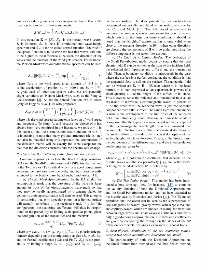
A. Returns in a simple bistatic configuration

In our first simulation (Fig. 6), we generated a sea surface

of 64 × 64 m with the exact same conditions as in Fig. 3.

We add a ship cruising with a heading of 35◦, having the

characteristics of a small motor boat (length of 10 m, beam

of 4 m, draft of 1.5 m and speed of 10 kt). The transmitter is

located at coordinates [x = 0, y = 0, z = 256.65] (in meters)

and the receiver is located at [x = 32.0, y = 0, z = 87.91]. The

antennas aim at the center of the tile, which yields θi = 20◦,

θs = 30◦ relatively to the mean sea surface, at the center.

The antennas are both rectangular, uniformly illuminated, with

a width of 18 cm and a breadth of 14 cm. We plotted in

figure 6.a the elevation map and in figure 6.b the modulus

of the received signal (when the transmitted signal is of unit

amplitude). Figures 6.c to 6.f show the scattering coefficients

σmn (in dB) for each individual scatterer of the sea. This

toy example nonetheless shows the clear influence of the

bistatic angles since the antennas are close to the surface: each

individual point of the surface will be lighted differently and

will contribute in a distinct way. Also, notice how the sea

scatters the energy even outside of the main antenna lobe,

especially for the co-polarized channels.

B. Synthetic Aperture Radar images

We generated various SAR images, with the following

setting: we used a canonical rectangular aperture, illuminated

uniformly, carried aboard a plane flying at 3,000 m at a

distance of 3,000 m from the center of the simulated tile of

sea. The antenna aims at the center of the tile. The plane speed

is 222 m.s−1 (800 km.h−1), the pulse repetition frequency is

equal to 222 Hz, hence a pulse is transmitted every meter.

The carrier is set to 10 GHz, and the signal is chirped on

75 MHz so as to obtain a range resolution of 2 m (pulse

duration: 333 ns); the antenna width is chosen so as to obtain

a comparable resolution in azimuth after beamforming. The

configuration is here monostatic, so as to be able to reuse

existing SAR software; however, bistatic SAR [17] may be

readily used as well.

In these experiments, for each transmitted pulse, the re-

flected signal for each elementary scatterer (“pixel”) is com-

puted and the corresponding signal is added to an array

representing the temporal raw signal that would be received for

the transmitted ping. Between each ping, the sea height map

is not recomputed; although it would be very possible, this

is a time-consuming process not really justified here because

the illumination time is very short, typically below 0.25 s,

which means that movement of the waves is negligible. The

total computation time for each pulse is of about 12 s (for a

512 × 512 mesh, with a 3 GHz Pentium IV, the simulation

code being written in C). Surprisingly enough, the bulk of the

a) b)

c) d)

e) f)

Fig. 6. Simulation 1

computation time is taken by the 10-lines-long loop writing

the pulse in the received signal array (despite aggressive

optimization), and not that part of the code which computes

the radar cross section of a sea element.

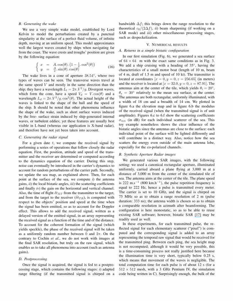
In simulation 2 (Fig. 7), we simulate a sea of state 2

(significant wave height: 0.5 m), with a wind direction of 55◦.

We add the same ship as in simulation 1. We use a mesh of

512 × 512 pixels to simulate a sea patch of length 128 m.

The arms of the wake are clearly visible and are very bright,

as compared to the level of the sea. Cross-polarized channels

HV and VH offer a better contrast than co-polarized channels,

which is usual when observing the sea. The spurious secondary

spikes are at least -27 dB below the answer of the wake and

are likely due to secondary lobes after range and amplitude

compression; in particular, since we took a constant antenna

illumination pattern in our example, the secondary (physical)

antenna lobes are not tapered off.

In simulation 3 (Fig. 8), we use the same setting, except

that the wind direction is 0◦ (thus blowing in the orthogonal

direction to the plane) and the ship has a heading of 45◦. The

signal to noise ratio between the wake and the sea is lower,

which makes sense in the monostatic configuration: when sea

waves travel in the look direction, the probability of finding a

small element of water reflecting rays towards the transmitter

is maximized, which means that the contribution of the sea is

more important. Also, we note that the VV channel gives the

strongest returns, which is usual when the incidence angle is

greater than about 20◦. Experiments 2 and 3 show that the

visibility of ship wakes is strongly influenced by both the

wind direction, the heading of the ship, and the direction of

observation; this shows that the observability of ship wakes is

by no means guaranteed.

Simulation 4 (Fig. 9) exhibits results that would be obtained

when looking at a sea of state 5-6 (the wind speed at 19.5 m is

10 m.s−1 i.e. about 19.43 kt, with a direction of 30◦). The tile

has a width of 500 m (512 × 512 scatterers). The significant

wave height of the waves is now of 2.95 m. In those images,

the shape of the waves is clearly visible; here again, the cross-

polarized channels yield the best contrast whereas the VV

channel gives the highest returns.

Fig. 7. Simulation 2

VI. CONCLUSION

We presented a simulator capable of producing pseudo-raw

radar signals which can be injected into existing or future

post-processing algorithms. This simulator will be used as

a tool to generate virtual scenes, so as to test various ship

detection and tracking scenarios, using monostatic or bistatic

radars. Also, this tool can be used to investigate the influence

of natural parameters such as the wind, the orientation of the

sensors, on the final images. Indeed, images can be simulated

without sensor noise, or, on the other hand, any parameter can

be perturbed at will so as to observe the effect on the final

image.

Fig. 8. Simulation 3

Fig. 9. Simulation 4

REFERENCES

[1] I. Antipov, “Analysis of sea clutter data,” Defence Science and Technol-ogy Organisation (Department of Defence, Australia), Tech. Rep. DSTO-TR-0647, Mar. 1998.

[2] H. Rohling, “Radar CFAR thresholding in clutter and multiple targetsituations,” IEEE Transactions on Aerospace and Electronic Systems,pp. 608–621, July 1983.

[3] A. Fung and K. K. Lee, “A semi-empirical sea-spectrum model forscattering coefficient estimation,” IEEE Journal of Oceanic Engineering,vol. 7, no. 4, pp. 166–176, 1982.

[4] C. Cochin, T. Landeau, G. Delhommeau, and B. Alessandrini, “Simula-tor of ocean scenes observed by polarimetric SAR,” in Proceedings of

the Comitee on Earth Observation Satellites SAR Workshop, Toulouse,France, Oct. 1999.

[5] G. Zilman and T. Miloh, “Radar backscatter of a V-like ship wake froma sea surface covered by surfactants,” in Proceedings of the Twenty First

Symposium on Naval Hydrodynamics, Trondheim, Norway, June 1996.[6] O. Airiau and A. Khenchaf, “A methodology for modelling and sim-

ulating target echoes with a moving polarimetric bistatic radar,” Radio

Science, vol. 35, no. 3, pp. 773–782, May-June 2000.[7] M. I. Skolnik, Radar Handbook. New York: McGraw-Hill Publishing

Company, 1970.[8] M. Saillard and A. Sentenac, “Rigorous solutions for electromagnetic

scattering from rough surfaces,” Waves in Random Media, vol. 11, pp.R103–R137, 2001.

[9] M. Tucker and E. Pitt, Waves in Ocean Engineering, ser. Elsevier OceanEngineering Book Series. Elsevier, 2001.

[10] M.S. Longuet-Higgins et al., Ocean Wave Spectra. Prentice-Hall, Inc.,1963, ch. Observations of the Directional Spectrum of Sea Waves Usingthe Motions of a Floating Buoy, pp. 111–136.

[11] A. Khenchaf and O. Airiau, “Bistatic radar moving returns from seasurface,” IEICE Transactions on Electronics, vol. E83-C, no. 12, Dec.2000.

[12] F. T. Ulaby, R. K. Moore, and A. K. Fung, Microwave Remote Sensing:

Active and Passive, vol. II. Artech House, 1986.[13] C. Cox and W. Munk, “Statistics of the sea surface derived from sun

glitter,” Journal of Marine Research, vol. 13, pp. 198–227, 1954.[14] A. Ishimaru, Wave Propagation and Scattering In Random Media (Vol.

2). Academic Press, 1978.[15] G. R. Valenzuela, “Theories for the interactions of electromagnetic and

oceanic waves – a review,” Boundary-Layer Meteorology, vol. 13, no.61-85, 1978.

[16] E. I. Thorsos and D. M. Jackson, “Studies of scattering theory usingnumerical methods,” Waves in Random Media, vol. 1, no. 3, p. S165,July 1991.

[17] F. Comblet, M. Y. Ayari, F. Pellen, and A. Khenchaf, “Bistatic radarimaging system for sea surface target detection,” in Proceedings of the

IEEE Conference on Oceans 2005 (Europe), Brest, France, June 2005.