Embed Size (px)
Citation preview
A SOCIALLY INTERACTIVE MULTIMODAL
HUMAN-ROBOT INTERACTION FRAMEWORK
THROUGH STUDIES ON MACHINE AND DEEP
LEARNING
JORDAN JAMES BIRD
Doctor of Philosophy
ASTON UNIVERSITY
February 2021
© Jordan James Bird, 2021
Jordan James Bird asserts their moral right to be identified as the author of this thesis
This copy of the thesis has been supplied on condition that anyone who consults it is understood to
recognise that its copyright belongs to its author and that no quotation from the thesis and no information
derived from it may be published without appropriate permission or acknowledgement.
1
Aston UniversityA Socially Interactive Multimodal Human-Robot Interaction Framework through Studies
on Machine and Deep Learning
Jordan James Bird
Doctor of Philosophy
2021
Abstract
In modern Human-Robot Interaction, much thought has been given to accessibility
regarding robotic locomotion, specifically the enhancement of awareness and lowering of
cognitive load. On the other hand, with social Human-Robot Interaction considered, pub-
lished research is far sparser given that the problem is less explored than pathfinding and
locomotion.
This thesis studies how one can endow a robot with affective perception for social aware-
ness in verbal and non-verbal communication. This is possible by the creation of a Human-
Robot Interaction framework which abstracts machine learning and artificial intelligence
technologies which allow for further accessibility to non-technical users compared to the
current State-of-the-Art in the field. These studies thus initially focus on individual robotic
abilities in the verbal, non-verbal and multimodality domains. Multimodality studies show
that late data fusion of image and sound can improve environment recognition, and simi-
larly that late fusion of Leap Motion Controller and image data can improve sign language
recognition ability. To alleviate several of the open issues currently faced by researchers in
the field, guidelines are reviewed from the relevant literature and met by the design and
structure of the framework that this thesis ultimately presents.
The framework recognises a user’s request for a task through a chatbot-like architecture.
Through research in this thesis that recognises human data augmentation (paraphrasing)
and subsequent classification via language transformers, the robot’s more advanced Natural
J. J. Bird, PhD Thesis, Aston University 2021 2
Language Processing abilities allow for a wider range of recognised inputs. That is, as
examples show, phrases that could be expected to be uttered during a natural human-
human interaction are easily recognised by the robot. This allows for accessibility to robotics
without the need to physically interact with a computer or write any code, with only the
ability of natural interaction (an ability which most humans have) required for access to all
the modular machine learning and artificial intelligence technologies embedded within the
architecture.
Following the research on individual abilities, this thesis then unifies all of the technolo-
gies into a deliberative interaction framework, wherein abilities are accessed from long-term
memory modules and short-term memory information such as the user’s tasks, sensor data,
retrieved models, and finally output information. In addition, algorithms for model improve-
ment are also explored, such as through transfer learning and synthetic data augmentation
and so the framework performs autonomous learning to these extents to constantly improve
its learning abilities. It is found that transfer learning between electroencephalographic and
electromyographic biological signals improves the classification of one another given their
slight physical similarities. Transfer learning also aids in environment recognition, when
transferring knowledge from virtual environments to the real world. In another example of
non-verbal communication, it is found that learning from a scarce dataset of American Sign
Language for recognition can be improved by multi-modality transfer learning from hand
features and images taken from a larger British Sign Language dataset. Data augmentation
is shown to aid in electroencephalographic signal classification by learning from synthetic
signals generated by a GPT-2 transformer model, and, in addition, augmenting training
with synthetic data also shows improvements when performing speaker recognition from
human speech.
Given the importance of platform independence due to the growing range of available
consumer robots, four use cases are detailed, and examples of behaviour are given by the
Pepper, Nao, and Romeo robots as well as a computer terminal. The use cases involve
a user requesting their electroencephalographic brainwave data to be classified by simply
asking the robot whether or not they are concentrating. In a subsequent use case, the user
asks if a given text is positive or negative, to which the robot correctly recognises the task
of natural language processing at hand and then classifies the text, this is output and the
physical robots react accordingly by showing emotion. The third use case has a request for
J. J. Bird, PhD Thesis, Aston University 2021 3
sign language recognition, to which the robot recognises and thus switches from listening
to watching the user communicate with them. The final use case focuses on a request
for environment recognition, which has the robot perform multimodality recognition of its
surroundings and note them accordingly.
The results presented by this thesis show that several of the open issues in the field
are alleviated through the technologies within, structuring of, and examples of interaction
with the framework. The results also show the achievement of the three main goals set out
by the research questions; the endowment of a robot with affective perception and social
awareness for verbal and non-verbal communication, whether we can create a Human-Robot
Interaction framework to abstract machine learning and artificial intelligence technologies
which allow for the accessibility of non-technical users, and, as previously noted, which
current issues in the field can be alleviated by the framework presented and to what extent.
J. J. Bird, PhD Thesis, Aston University 2021 4

This work is dedicated to all of those who have supported me during my journey through
education.
Most especially my parents and sister for their unconditional support and endless
enthusiasm for my work throughout my research activities and PhD studies.
I would also like to specially thank Mr. Carl Sheen, for I would not find myself writing any
of this if it were not for his belief in my ability ten years ago.
J. J. Bird, PhD Thesis, Aston University 2021 5
CONTENTS
Contents
1 Introduction 21
1.1 Motivation and Objectives . . . . . . . . . . . . . . . . . . . . . . . . . . . . 23
1.2 Scientific Contributions and Research Questions . . . . . . . . . . . . . . . . 24
1.2.1 Scientific Novelty . . . . . . . . . . . . . . . . . . . . . . . . . . . . . 27
1.3 Thesis Organisation . . . . . . . . . . . . . . . . . . . . . . . . . . . . . . . 28
2 Human-Robot Interaction 30
2.1 Introduction . . . . . . . . . . . . . . . . . . . . . . . . . . . . . . . . . . . . 30
2.2 Emergence of Robotic Behaviour . . . . . . . . . . . . . . . . . . . . . . . . 32
2.3 Open Issues in HRI . . . . . . . . . . . . . . . . . . . . . . . . . . . . . . . . 34
2.4 Phonetic Speech Recognition . . . . . . . . . . . . . . . . . . . . . . . . . . 35
2.5 Speaker Recognition and Synthesis . . . . . . . . . . . . . . . . . . . . . . . 39
2.6 Accent Recognition . . . . . . . . . . . . . . . . . . . . . . . . . . . . . . . . 40
2.7 Sign Language Recognition . . . . . . . . . . . . . . . . . . . . . . . . . . . 42
2.8 Sentiment Analysis . . . . . . . . . . . . . . . . . . . . . . . . . . . . . . . . 45
2.9 EEG and EMG Recognition . . . . . . . . . . . . . . . . . . . . . . . . . . . 46
2.10 Biosignal Augmentation and Transfer . . . . . . . . . . . . . . . . . . . . . 48
2.11 Chatbot Interaction . . . . . . . . . . . . . . . . . . . . . . . . . . . . . . . 51
2.12 Scene Recognition and Sim2Real . . . . . . . . . . . . . . . . . . . . . . . . 52
2.13 Summary . . . . . . . . . . . . . . . . . . . . . . . . . . . . . . . . . . . . . 55
3 Key Concepts in Machine Learning 56
3.1 Introduction . . . . . . . . . . . . . . . . . . . . . . . . . . . . . . . . . . . . 56
3.2 Validation Testing . . . . . . . . . . . . . . . . . . . . . . . . . . . . . . . . 56
3.3 Attribute Selection . . . . . . . . . . . . . . . . . . . . . . . . . . . . . . . . 57
J. J. Bird, PhD Thesis, Aston University 2021 6
CONTENTS
3.4 Classical Models . . . . . . . . . . . . . . . . . . . . . . . . . . . . . . . . . 58
3.4.1 Decision Trees . . . . . . . . . . . . . . . . . . . . . . . . . . . . . . 58
3.4.2 Support Vector Machines . . . . . . . . . . . . . . . . . . . . . . . . 59
3.4.3 Naıve Bayes . . . . . . . . . . . . . . . . . . . . . . . . . . . . . . . . 59
3.4.4 Bayesian Networks . . . . . . . . . . . . . . . . . . . . . . . . . . . . 60
3.4.5 Hidden Markov Models . . . . . . . . . . . . . . . . . . . . . . . . . 60
3.4.6 Logistic Regression . . . . . . . . . . . . . . . . . . . . . . . . . . . . 61
3.4.7 Nearest Neighbour Classification . . . . . . . . . . . . . . . . . . . . 61
3.4.8 Linear and Quadratic Discriminant Analysis . . . . . . . . . . . . . . 62
3.4.9 Gradient Boosting . . . . . . . . . . . . . . . . . . . . . . . . . . . . 62
3.5 Deep Learning . . . . . . . . . . . . . . . . . . . . . . . . . . . . . . . . . . 63
3.5.1 Multilayer Perceptron . . . . . . . . . . . . . . . . . . . . . . . . . . 64
3.5.2 Convolutional Layers . . . . . . . . . . . . . . . . . . . . . . . . . . . 65
3.5.3 Long Short-Term Memory Layers . . . . . . . . . . . . . . . . . . . . 65
3.5.4 Transformer Based Models . . . . . . . . . . . . . . . . . . . . . . . 67
3.5.5 Momentum . . . . . . . . . . . . . . . . . . . . . . . . . . . . . . . . 67
3.6 Ensemble Learning . . . . . . . . . . . . . . . . . . . . . . . . . . . . . . . . 68
3.6.1 Adaptive Boosting . . . . . . . . . . . . . . . . . . . . . . . . . . . . 69
3.6.2 Voting . . . . . . . . . . . . . . . . . . . . . . . . . . . . . . . . . . . 69
3.6.3 Random Forests . . . . . . . . . . . . . . . . . . . . . . . . . . . . . 70
3.6.4 Stacking . . . . . . . . . . . . . . . . . . . . . . . . . . . . . . . . . . 70
3.7 Errors . . . . . . . . . . . . . . . . . . . . . . . . . . . . . . . . . . . . . . . 70
3.8 Evolutionary Topology Search . . . . . . . . . . . . . . . . . . . . . . . . . . 71
3.9 Transfer Learning . . . . . . . . . . . . . . . . . . . . . . . . . . . . . . . . . 74
3.10 Data Augmentation . . . . . . . . . . . . . . . . . . . . . . . . . . . . . . . 76
3.11 Summary . . . . . . . . . . . . . . . . . . . . . . . . . . . . . . . . . . . . . 77
4 Verbal Human-Robot Interaction 79
4.1 Introduction . . . . . . . . . . . . . . . . . . . . . . . . . . . . . . . . . . . . 79
4.2 Feature Extraction from Audio . . . . . . . . . . . . . . . . . . . . . . . . . 79
4.3 Synthetic Data Augmentation for Speaker Recognition . . . . . . . . . . . . 80
4.3.1 Method . . . . . . . . . . . . . . . . . . . . . . . . . . . . . . . . . . 82
J. J. Bird, PhD Thesis, Aston University 2021 7
CONTENTS
4.3.2 Results . . . . . . . . . . . . . . . . . . . . . . . . . . . . . . . . . . 86
4.4 Multi-objective Evolutionary Phonetic Speech Recognition . . . . . . . . . . 95
4.4.1 Method . . . . . . . . . . . . . . . . . . . . . . . . . . . . . . . . . . 98
4.4.2 Results . . . . . . . . . . . . . . . . . . . . . . . . . . . . . . . . . . 100
4.5 Accent Classification of Human Speech . . . . . . . . . . . . . . . . . . . . . 108
4.5.1 Method . . . . . . . . . . . . . . . . . . . . . . . . . . . . . . . . . . 109
4.5.2 Results . . . . . . . . . . . . . . . . . . . . . . . . . . . . . . . . . . 111
4.6 Phonetic Speech Synthesis . . . . . . . . . . . . . . . . . . . . . . . . . . . . 112
4.6.1 Method . . . . . . . . . . . . . . . . . . . . . . . . . . . . . . . . . . 113
4.6.2 Results . . . . . . . . . . . . . . . . . . . . . . . . . . . . . . . . . . 117
4.7 High Resolution Sentiment Analysis by Ensemble Classification . . . . . . . 119
4.7.1 Method . . . . . . . . . . . . . . . . . . . . . . . . . . . . . . . . . . 120
4.7.2 Results . . . . . . . . . . . . . . . . . . . . . . . . . . . . . . . . . . 121
4.8 Summary and Conclusion . . . . . . . . . . . . . . . . . . . . . . . . . . . . 123
5 Non-Verbal Human-Robot Interaction 131
5.1 Introduction . . . . . . . . . . . . . . . . . . . . . . . . . . . . . . . . . . . . 131
5.2 Biosignal Processing . . . . . . . . . . . . . . . . . . . . . . . . . . . . . . . 132
5.2.1 Electroencephalography . . . . . . . . . . . . . . . . . . . . . . . . . 132
5.2.2 Electromyography . . . . . . . . . . . . . . . . . . . . . . . . . . . . 134
5.2.3 Feature Extraction . . . . . . . . . . . . . . . . . . . . . . . . . . . . 137
5.3 An Evolutionary Approach to Brain-machine Interaction . . . . . . . . . . . 140
5.3.1 Method . . . . . . . . . . . . . . . . . . . . . . . . . . . . . . . . . . 141
5.3.2 Results . . . . . . . . . . . . . . . . . . . . . . . . . . . . . . . . . . 144
5.4 CNN Classification of EEG Signals represented in 2D and 3D . . . . . . . . 155
5.4.1 Method . . . . . . . . . . . . . . . . . . . . . . . . . . . . . . . . . . 157
5.4.2 Results . . . . . . . . . . . . . . . . . . . . . . . . . . . . . . . . . . 161
5.5 Real-time EMG classification via Inductive and Supervised Transductive
Transfer Learning . . . . . . . . . . . . . . . . . . . . . . . . . . . . . . . . . 172
5.5.1 Method . . . . . . . . . . . . . . . . . . . . . . . . . . . . . . . . . . 174
5.5.2 Results . . . . . . . . . . . . . . . . . . . . . . . . . . . . . . . . . . 175
J. J. Bird, PhD Thesis, Aston University 2021 8
CONTENTS
5.6 Data Augmentation by Synthetic Biological Signals Machine-generated by
GPT-2 . . . . . . . . . . . . . . . . . . . . . . . . . . . . . . . . . . . . . . . 183
5.6.1 Method . . . . . . . . . . . . . . . . . . . . . . . . . . . . . . . . . . 184
5.6.2 Results . . . . . . . . . . . . . . . . . . . . . . . . . . . . . . . . . . 187
5.7 Cross-Domain MLP and CNN Transfer Learning for Biological Signal Pro-
cessing . . . . . . . . . . . . . . . . . . . . . . . . . . . . . . . . . . . . . . . 189
5.7.1 Method . . . . . . . . . . . . . . . . . . . . . . . . . . . . . . . . . . 190
5.7.2 Method I: MLP Transfer Learning . . . . . . . . . . . . . . . . . . . 191
5.7.3 Method II: CNN Transfer Learning . . . . . . . . . . . . . . . . . . . 193
5.7.4 Results . . . . . . . . . . . . . . . . . . . . . . . . . . . . . . . . . . 194
5.7.5 Experiment I: MLP Transfer Learning . . . . . . . . . . . . . . . . . 195
5.7.6 Experiment II: CNN Transfer Learning . . . . . . . . . . . . . . . . 197
5.8 Summary and Conclusion . . . . . . . . . . . . . . . . . . . . . . . . . . . . 199
6 Multimodality Human-Robot Interaction 206
6.1 Introduction . . . . . . . . . . . . . . . . . . . . . . . . . . . . . . . . . . . . 206
6.2 Multimodality Late Fusion for Scene Classification . . . . . . . . . . . . . . 206
6.2.1 Method . . . . . . . . . . . . . . . . . . . . . . . . . . . . . . . . . . 209
6.2.2 Results . . . . . . . . . . . . . . . . . . . . . . . . . . . . . . . . . . 212
6.3 CNN transfer learning for Scene Classification . . . . . . . . . . . . . . . . . 217
6.3.1 Method . . . . . . . . . . . . . . . . . . . . . . . . . . . . . . . . . . 219
6.3.2 Results . . . . . . . . . . . . . . . . . . . . . . . . . . . . . . . . . . 221
6.4 Sign Language Recognition via Late Fusion of Computer Vision and Leap
Motion . . . . . . . . . . . . . . . . . . . . . . . . . . . . . . . . . . . . . . . 224
6.4.1 Method . . . . . . . . . . . . . . . . . . . . . . . . . . . . . . . . . . 225
6.4.2 Results . . . . . . . . . . . . . . . . . . . . . . . . . . . . . . . . . . 233
6.5 Summary and Conclusion . . . . . . . . . . . . . . . . . . . . . . . . . . . . 239
7 Integration into a Human-Robot Interaction Framework 244
7.1 Introduction . . . . . . . . . . . . . . . . . . . . . . . . . . . . . . . . . . . . 244
7.2 Chatbot Interface: Human Data Augmentation with T5 and Transformer
Ensemble . . . . . . . . . . . . . . . . . . . . . . . . . . . . . . . . . . . . . 244
7.2.1 Method . . . . . . . . . . . . . . . . . . . . . . . . . . . . . . . . . . 247
J. J. Bird, PhD Thesis, Aston University 2021 9
CONTENTS
7.2.2 Results . . . . . . . . . . . . . . . . . . . . . . . . . . . . . . . . . . 253
7.3 An Integrated HRI Framework . . . . . . . . . . . . . . . . . . . . . . . . . 263
7.4 Use Cases . . . . . . . . . . . . . . . . . . . . . . . . . . . . . . . . . . . . . 266
7.4.1 Use Case 1: Am I concentrating? . . . . . . . . . . . . . . . . . . . . 268
7.4.2 Use Case 2: Is this review good or bad? . . . . . . . . . . . . . . . . 269
7.4.3 Use Case 3: Can you help me learn Sign Language? . . . . . . . . . 271
7.4.4 Use Case 4: Where are you? . . . . . . . . . . . . . . . . . . . . . . 272
7.5 Summary and Conclusion . . . . . . . . . . . . . . . . . . . . . . . . . . . . 274
8 Discussion and Conclusion 276
8.1 Revisiting Open Issues . . . . . . . . . . . . . . . . . . . . . . . . . . . . . . 276
8.1.1 Adaptability and ease of use . . . . . . . . . . . . . . . . . . . . . . 276
8.1.2 Provision of overall framework . . . . . . . . . . . . . . . . . . . . . 277
8.1.3 Extendibility . . . . . . . . . . . . . . . . . . . . . . . . . . . . . . . 278
8.1.4 Shared and centralised knowledge representation . . . . . . . . . . . 278
8.1.5 Open software . . . . . . . . . . . . . . . . . . . . . . . . . . . . . . 278
8.1.6 Enhancement of awareness . . . . . . . . . . . . . . . . . . . . . . . 279
8.1.7 Lowering of cognitive load . . . . . . . . . . . . . . . . . . . . . . . . 279
8.1.8 Increase of efficiency . . . . . . . . . . . . . . . . . . . . . . . . . . . 280
8.1.9 Provide help . . . . . . . . . . . . . . . . . . . . . . . . . . . . . . . 280
8.2 Research Questions Revisited . . . . . . . . . . . . . . . . . . . . . . . . . . 281
8.2.1 Research Question 1 . . . . . . . . . . . . . . . . . . . . . . . . . . . 281
8.2.2 Research Question 2 . . . . . . . . . . . . . . . . . . . . . . . . . . . 283
8.2.3 Research Question 3 . . . . . . . . . . . . . . . . . . . . . . . . . . . 284
8.3 Research Limitations and Future Work . . . . . . . . . . . . . . . . . . . . . 285
8.4 Conclusion . . . . . . . . . . . . . . . . . . . . . . . . . . . . . . . . . . . . 286
8.5 Ethics Statement . . . . . . . . . . . . . . . . . . . . . . . . . . . . . . . . . 287
A List Publications during PhD Study 315
J. J. Bird, PhD Thesis, Aston University 2021 10
LIST OF FIGURES
List of Figures
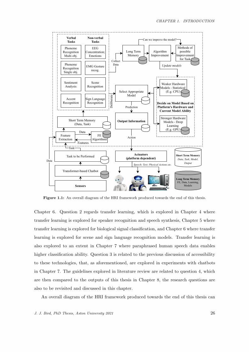
1.1 An overall diagram of the HRI framework produced towards the end of this thesis. . . . . . . 26
1.2 Overview of the relationship between Chapters, Research Questions (RQ), and Objectives
(OBJ). . . . . . . . . . . . . . . . . . . . . . . . . . . . . . . . . . . . . . . . . . . . . . . . . . 28
2.1 A 32-bit OpenBCI Cyton Biosensing Board. . . . . . . . . . . . . . . . . . . . . . . . . . . . . 46
3.1 Flow Diagram of the evolutionary search of Neural Network topology. Population size is given
as p and fitness calculation is given as F. Set {b1..bn} denotes the best solution presented at
each generation. . . . . . . . . . . . . . . . . . . . . . . . . . . . . . . . . . . . . . . . . . . . . 73
3.2 Example of a successful Transfer Learning experiment. Transfer Learning (top line) has a
higher starting point, steeper curve, and higher asymptote in comparison to learning via
random weight distribution (bottom line). . . . . . . . . . . . . . . . . . . . . . . . . . . . . . 74
3.3 A real image of the Pepper Robot (left) followed by four examples of augmented images.
Augmentation techniques involve offsets, scaling, rotation and mirroring. . . . . . . . . . . . . 76
4.1 A diagram of the experimental method in this work. The two networks being directly com-
pared are classifying the same data, with the difference that the initial weight distribution
is either from standard random distribution or transfer learning from GPT-2 and LSTM
produced synthetic data. . . . . . . . . . . . . . . . . . . . . . . . . . . . . . . . . . . . . . . . 83
4.2 The training processes of the best performing models in terms of loss, separated for readability
purposes. Results are given for a benchmarking experiment on all of the dataset rather than
an individual. . . . . . . . . . . . . . . . . . . . . . . . . . . . . . . . . . . . . . . . . . . . . . 86
4.3 The training processes of LSTMs with 64, 256, and 512 units in 1-3 hidden layers, separated
for readability purposes. Results are given for a benchmarking experiment on all of the dataset
rather than an individual. . . . . . . . . . . . . . . . . . . . . . . . . . . . . . . . . . . . . . . 87
4.4 The training process of the GPT-2 model. Results are given for a benchmarking experiment
on all of the dataset rather than an individual. . . . . . . . . . . . . . . . . . . . . . . . . . . 87
4.5 Description of the training and prediction process applied in this study. Initial training
happens to the left of the trained model where phonemes are used as data objects for learning
and validated through 10-fold cross-validation; prediction of unknown phonemes from sound
data occurs to the right of the model. . . . . . . . . . . . . . . . . . . . . . . . . . . . . . . . 98
J. J. Bird, PhD Thesis, Aston University 2021 11
LIST OF FIGURES
4.6 Benchmarking of HMM hidden units. . . . . . . . . . . . . . . . . . . . . . . . . . . . . . . . . 100
4.7 Single-objective optimisation of single hidden layer neural networks. The dashed line denotes
the HMM. . . . . . . . . . . . . . . . . . . . . . . . . . . . . . . . . . . . . . . . . . . . . . . . 103
4.8 A comparison of model training time for produced models post-search. S1-S3 are from Table
4.10 and S4-S6 are from Table 4.11. . . . . . . . . . . . . . . . . . . . . . . . . . . . . . . . . 104
4.9 Evolution of accuracy for multi-objective algorithms. A value of 16.33 is omitted for purposes
of readability. . . . . . . . . . . . . . . . . . . . . . . . . . . . . . . . . . . . . . . . . . . . . . 105
4.10 Evolution of resource usage for multi-objective algorithms. The dashed line denotes the HMM.105
4.11 Final results presented by the multi-objective searches. . . . . . . . . . . . . . . . . . . . . . . 106
4.12 Information Gain of each MFCC log attribute in the dataset. . . . . . . . . . . . . . . . . . . 109
4.13 Exploration of HMM hidden unit selection. . . . . . . . . . . . . . . . . . . . . . . . . . . . . 110
4.14 Exploration of LSTM hidden unit selection. . . . . . . . . . . . . . . . . . . . . . . . . . . . . 111
4.15 Spectrogram of “Working at a University is an Enlightening Experience” when spoken by a
human being. . . . . . . . . . . . . . . . . . . . . . . . . . . . . . . . . . . . . . . . . . . . . 115
4.16 Spectrogram of “Working at a University is an Enlightening Experience” when predicted by
the English written text Tacotron network. . . . . . . . . . . . . . . . . . . . . . . . . . . . . 116
4.17 Spectrogram of “Working at a University is an Enlightening Experience” when predicted by
the phonetically aware Tacotron network. . . . . . . . . . . . . . . . . . . . . . . . . . . . . . 116
4.18 Comparison of the two approaches for the average of ten Sets of three experiments. . . . . . . 119
4.19 Error matrix for the classifications given by the best model, a Vote(RF, NBM, MLP) . . . . . 122
5.1 The Muse EEG headband. . . . . . . . . . . . . . . . . . . . . . . . . . . . . . . . . . . . . . . 133
5.2 EEG sensors TP9, AF7, AF8 and TP10 of the Muse headband on the international standard
EEG placement system. . . . . . . . . . . . . . . . . . . . . . . . . . . . . . . . . . . . . . . . 134
5.3 The MYO EMG armband. . . . . . . . . . . . . . . . . . . . . . . . . . . . . . . . . . . . . . . 135
5.4 A graphical representation of the Deep Evolutionary (DEvo) approach to complex signal
classification. An evolutionary algorithm simulation selects a set of natural features before a
similar approach is used, then this feature set becomes the input to optimise a bioinspired
classifier. . . . . . . . . . . . . . . . . . . . . . . . . . . . . . . . . . . . . . . . . . . . . . . . . 142
5.5 A subject having their EEG brainwave data recorded while being exposed to a stimulus with
an emotional valence. . . . . . . . . . . . . . . . . . . . . . . . . . . . . . . . . . . . . . . . . . 144
5.6 Three evolutionary algorithm simulations to optimise an MLP for the Mental State dataset. . 147
5.7 Three evolutionary algorithm simulations to optimise an MLP for the Emotional State dataset.149
5.8 Three evolutionary algorithm simulations to optimise an MLP for the MindBigData dataset. 149
5.9 Manual tuning of LSTM topology for Mental State (MS), Emotional State (ES) and Mind-
BigData (MBD) classification. . . . . . . . . . . . . . . . . . . . . . . . . . . . . . . . . . . . 152
5.10 Graph to show the time taken to build the final models post-search. . . . . . . . . . . . . . . 153
5.11 Final results for the experiment. . . . . . . . . . . . . . . . . . . . . . . . . . . . . . . . . . . 154
J. J. Bird, PhD Thesis, Aston University 2021 12
LIST OF FIGURES
5.12 Overview of the methodology. EEG signals are processed into 2D or 3D data benchmarked
by a 2D or 3D CNN. Three different attribute selection processes are explored. Finally, the
best models have their interpretation topologies optimised heuristically for a final best result. 157
5.13 Thirty samples of attention state EEG data displayed as 27x27 Images. Row one shows
relaxed data, two shows neutral data, and the third row shows concentrating data. . . . . . 160
5.14 Three attention state samples rendered as 9x9x9 cubes of voxels. Leftmost cube is relaxed,
centre is neutral, and the rightmost cube represents concentrating data. . . . . . . . . . . . . 160
5.15 Thirty samples of emotional state EEG data displayed as 27x27 images. Row one shows
negative valence data, two shows neutral data, and the third row shows positive valence data. 160
5.16 Three emotional state samples rendered as 9x9x9 cubes of voxels. Leftmost cube is negative
valence, centre is neutral, and the rightmost cube represents positive valence data. . . . . . . 160
5.17 Twenty samples of eye state EEG data displayed as 27x27 images. Row one shows eyes open,
row two shows eyes closed. . . . . . . . . . . . . . . . . . . . . . . . . . . . . . . . . . . . . . 164
5.18 Two eye state EEG samples rendered as 9x9x9 cubes of voxels. Left cube is eyes open and
right is eyes closed. . . . . . . . . . . . . . . . . . . . . . . . . . . . . . . . . . . . . . . . . . 164
5.19 Evolutionary improvement of DEvoCNN for the attention state classification problem. . . . . 165
5.20 Evolutionary search of network topologies for the emotional state classification problem. . . . 166
5.21 Evolutionary search of network topologies for the eye state classification problem. . . . . . . . 166
5.22 Normalised confusion matrix for the unseen concentration data. . . . . . . . . . . . . . . . . . 168
5.23 Normalised confusion matrix for the unseen emotions data. . . . . . . . . . . . . . . . . . . . 169
5.24 Normalised confusion matrix for the unseen eye state data. . . . . . . . . . . . . . . . . . . . 169
5.25 Benchmarking of vote (best two) model generalisation ability for unseen data segments per
subject, in which generalisation has failed due to low classification accuracies. . . . . . . . . . 178
5.26 Initial pre-calibration mean generalisation ability of models on unseen data from four subjects
in a three-class scenario. Time is given for total data observed equally for three classes.
Generalisation has failed. . . . . . . . . . . . . . . . . . . . . . . . . . . . . . . . . . . . . . . 179
5.27 Confusion matrix for the random forest once calibrated, based on Table 5.29. . . . . . . . . . 180
5.28 Softbank Robotics’ Pepper robot playing 20 Questions with a human through real-time EMG
signal classification. . . . . . . . . . . . . . . . . . . . . . . . . . . . . . . . . . . . . . . . . . . 182
5.29 Initial training of the GPT-2 model and then generating a dataset of synthetic biological signals.184
5.30 The standard K-Fold cross validation process with the GPT-2 generated synthetic data being
introduced as additional training data for each fold. . . . . . . . . . . . . . . . . . . . . . . . 184
5.31 Comparison of GPT-2 generated (left) and genuine recorded (right) EEG data across “Concen-
trating”, “Relaxed”, and “Neutral” mental state classes. AF8 electrode readings are omitted
for readability purposes. . . . . . . . . . . . . . . . . . . . . . . . . . . . . . . . . . . . . . . . 185
5.32 Comparison of Power Spectral Densities of GPT-2 generated (left) and genuine recorded
(right) EEG data. For readability, only the PSD computed from electrode TP9 is shown. . . 186
5.33 Data collection from a male subject via the Myo armband on their left arm. . . . . . . . . . . 191
J. J. Bird, PhD Thesis, Aston University 2021 13
LIST OF FIGURES
5.34 30 Samples of EEG as 31x31 Images. Top row shows relaxed, middle row shows neutral, and
bottom row shows concentrating. . . . . . . . . . . . . . . . . . . . . . . . . . . . . . . . . . . 193
5.35 40 Samples of EMG as 31x31 Images. Top row shows close fist, second row shows open fingers,
third row shows wave in and bottom row shows wave out. . . . . . . . . . . . . . . . . . . . . 193
5.36 Highest (best) fitness observed per generation of the combined and normalised fitnesses of EEG
and EMG data classification. The two fitness components are considered equally weighted to
produce the same topology in order to allow direct transfer of weights. . . . . . . . . . . . . . 195
5.37 Test and training accuracies of EMG, EEG, and transfer between EMG and EEG. ‘EEG
Transfer’ denotes EMG to EEG and likewise for ‘EMG Transfer’. . . . . . . . . . . . . . . . . 196
5.38 Test and training accuracies of EMG, EEG, and transfer between EMG and EEG with a
Convolutional Neural Network, over 100 epochs. As with the previous figure, ‘EEG Transfer’
denotes EMG to EEG and likewise for ‘EMG Transfer’. . . . . . . . . . . . . . . . . . . . . . 198
6.1 Overview of the multi-modality network. Pre-trained networks without softmax activation
layer take synchronised images and audio segments as input, and classify based on interpre-
tations of the outputs of the two models. . . . . . . . . . . . . . . . . . . . . . . . . . . . . . . 207
6.2 Example of extracted data from a five second timeline. Each second, a frame is extracted
from the video along with the accompanying second of audio. . . . . . . . . . . . . . . . . . . 210
6.3 Image 10-fold classification ability with regards to interpretation neurons. . . . . . . . . . . . 212
6.4 Optimisation of audio classification network topologies. Final results of each are given in
Table 6.1. . . . . . . . . . . . . . . . . . . . . . . . . . . . . . . . . . . . . . . . . . . . . . . . 213
6.5 Multi-modality 10-fold classification ability with regards to interpretation neurons. . . . . . . 214
6.6 Sonograms of two short samples of audio files from a crowded beach and restaurant, human
speech occurs in both and due to this the single-modality audio classifier can confuse the two. 214
6.7 An example of confusion of the vision model, which is corrected through multi-modality. In
the second frame, the image of hair is incorrectly classified as the “FOREST” environment
through Computer Vision. . . . . . . . . . . . . . . . . . . . . . . . . . . . . . . . . . . . . . . 214
6.8 An example of confusion of the audio model, which is corrected through multi-modality. In
both examples, the audio of a City is incorrectly classified as the “RIVER” environment due
to the sounds of a fountain and flowing water by the audio classification network. . . . . . . . 215
6.9 Confusion matrix for the multi-modality model applied to completely unseen data (two min-
utes per class). . . . . . . . . . . . . . . . . . . . . . . . . . . . . . . . . . . . . . . . . . . . . 216
6.10 In order to collect artificial data, a camera is attached to a humanoid robot for height reference
in the Unity game engine. . . . . . . . . . . . . . . . . . . . . . . . . . . . . . . . . . . . . . . 219
6.11 Samples of virtual (top) and real (bottom) environments from the two datasets gathered for
these experiments. . . . . . . . . . . . . . . . . . . . . . . . . . . . . . . . . . . . . . . . . . . 220
6.12 Overall diagram of the experiment showing the derivation of ∆S and ∆F (change in starting
and final classification ability) for comparison. . . . . . . . . . . . . . . . . . . . . . . . . . . . 221
J. J. Bird, PhD Thesis, Aston University 2021 14
LIST OF FIGURES
6.13 An overall diagram of the three benchmarking experiments. Above shows the process of image
classification and below shows Leap Motion data classification for the same problem of sign
language recognition. The higher order function network shows the late fusion of the two to
form a multi-modality solution. . . . . . . . . . . . . . . . . . . . . . . . . . . . . . . . . . . . 226
6.14 Photograph and labelled sketch of the stereoscopic infrared camera array within a Leap Motion
Controller, illuminated by three infrared LEDs. . . . . . . . . . . . . . . . . . . . . . . . . . . 227
6.15 Screenshot of the view from Leap’s two infrared cameras and the detected hand reproduced
in 3D. Note that this study uses a front-facing view rather than up-facing as shown in the
screenshot. . . . . . . . . . . . . . . . . . . . . . . . . . . . . . . . . . . . . . . . . . . . . . . 227
6.16 An example of one second of RGB image data collected at a frequency of 0.2s per frame
(5Hz). Alongside each image that is taken, a numerical vector is collected from the Leap
Motion Controller. . . . . . . . . . . . . . . . . . . . . . . . . . . . . . . . . . . . . . . . . . . 227
6.17 Labelled diagram of the bone data detected by the Leap Motion sensor. Metacarpal bones
are not rendered by the LMC Visualiser. . . . . . . . . . . . . . . . . . . . . . . . . . . . . . . 228
6.18 The sign for ‘Hello’ in British Sign Language. . . . . . . . . . . . . . . . . . . . . . . . . . . . 230
6.19 The sign for ‘Hello’ in American Sign Language. . . . . . . . . . . . . . . . . . . . . . . . . . 230
6.20 Feature extraction from the RGB branch of the network, the input image is passed through a
fine-tuned VGG16 CNN and then a layer of 128 ReLu neurons provide output. The network
is trained via softmax output, but this softmax layer is later removed and the 128 outputs
are used in late fusion with the Leap Motion network. . . . . . . . . . . . . . . . . . . . . . . 231
6.21 Transfer learning experiments which train on BSL and produce initial starting weight distri-
butions for the ASL models. . . . . . . . . . . . . . . . . . . . . . . . . . . . . . . . . . . . . . 232
6.22 Mean Image 10-fold classification accuracy corresponding to interpretation neuron numbers. . 233
6.23 Three executions of optimisation of Neural Network topologies via an evolutionary algorithm. 234
6.24 Multi-modality 10-fold classification accuracy corresponding to interpretation neuron numbers
towards benchmarking the late-fusion network. . . . . . . . . . . . . . . . . . . . . . . . . . . 235
6.25 Confusion matrix for the best model (multi-modality, 76.5%) on the set of unseen data (not
present during training). . . . . . . . . . . . . . . . . . . . . . . . . . . . . . . . . . . . . . . . 237
7.1 A general overview of the proposed approach. . . . . . . . . . . . . . . . . . . . . . . . . . . . 245
7.2 Overall view of the Chatbot Interaction with Artificial Intelligence (CI-AI) system as a looped
process guided by human input, through natural social interaction due to the language trans-
former approach. The chatbot itself is trained via the process in Figure 7.3. . . . . . . . . . . 249
7.3 Data collection and model training process. In this example, the T5 paraphrasing model
is used to augment and enhance the training dataset. Models are compared when they are
augmented and when they are not on the same validation set, in order to discern what affect
augmentation has. . . . . . . . . . . . . . . . . . . . . . . . . . . . . . . . . . . . . . . . . . . 249
7.4 A stacking ensemble strategy where statistical machine learning models trained on the pre-
dictions of the transformers then classify the text based on the test data predictions of the
transformer classification models. . . . . . . . . . . . . . . . . . . . . . . . . . . . . . . . . . . 252
J. J. Bird, PhD Thesis, Aston University 2021 15
LIST OF FIGURES
7.5 Comparison of each model’s classification ability and number of million trainable parameters
within them. . . . . . . . . . . . . . . . . . . . . . . . . . . . . . . . . . . . . . . . . . . . . . 254
7.6 Normalised confusion matrix for the best command classification model, RoBERTa trained
on human data and augmented T5 paraphrased data. . . . . . . . . . . . . . . . . . . . . . . 255
7.7 Exploration and explanation for the errors made during validation which had a loss >1 (five
such cases). . . . . . . . . . . . . . . . . . . . . . . . . . . . . . . . . . . . . . . . . . . . . . . 258
7.8 Exploration of the best performing model by presenting unseen sentences and explaining
predictions. Green denotes useful features and red denotes features useful for another class
(detrimental to probability). . . . . . . . . . . . . . . . . . . . . . . . . . . . . . . . . . . . . . 260
7.9 Normalised confusion matrix for the best ensemble methods of Logistic Regression and Ran-
dom Forest (errors made by the two were identical). . . . . . . . . . . . . . . . . . . . . . . . 263
7.10 Overview of the HRI framework that unifies the individual studies performed within the prior
sections of this thesis. Following task selection via transformer-based classification of the input
medium, the task is then performed by the device such as a robot or computer terminal. In
learning mode, the data is also collected and algorithm improvement is performed through
searching methods of possible improvement and then updating models. . . . . . . . . . . . . . 264
7.11 Normalised confusion matrix of the extended classes dataset for the use cases of the HRI
framework. . . . . . . . . . . . . . . . . . . . . . . . . . . . . . . . . . . . . . . . . . . . . . . 267
7.12 Top features within the phrase for EEG concentration level classification. . . . . . . . . . . . 268
7.13 An example activity wherein a Romeo robot performs and subsequently reacts to EEG clas-
sification (relaxed, neutral, concentrating). . . . . . . . . . . . . . . . . . . . . . . . . . . . . . 269
7.14 Top features within the phrase for multi-level sentiment analysis of a text. . . . . . . . . . . . 269
7.15 An example activity leading to Pepper’s reaction and physical animation due to sentiment
analysis of a given text. . . . . . . . . . . . . . . . . . . . . . . . . . . . . . . . . . . . . . . . 270
7.16 Top features within the text for the classification of a request to use sign language. . . . . . . 271
7.17 An example behaviour for Nao, where the robot has a brief conversation via British Sign
Language Recognition as input, outputting speech audio accompanied by on-screen text.
None of the Alebaran Robots are capable of performing signs due to their limited hand joints. 272
7.18 Top features within the text for the classification of a scene recognition task. . . . . . . . . . 272
7.19 Predictions for real-time environmental recognition. In the first instance, three of the four
images are classified correctly. Following fine-tuning from the addition of additional data
objects, all four of the images are classified correctly. . . . . . . . . . . . . . . . . . . . . . . . 273
J. J. Bird, PhD Thesis, Aston University 2021 16
LIST OF TABLES
List of Tables
2.1 The seven diphthong vowels in spoken English language in terms of their phonetic symbols
and examples. . . . . . . . . . . . . . . . . . . . . . . . . . . . . . . . . . . . . . . . . . . . . . 36
2.2 Other state of the art works in autonomous Sign Language Recognition, indirectly compared
due to operation on different datasets and with different sensors. Note: it was observed in
this study that classification of unseen data is often lower than results found during training,
but many works do not benchmark this activity. . . . . . . . . . . . . . . . . . . . . . . . . . 44
4.1 Information regarding the data collection from the seven subjects of the Harvard Sentences.
Real Data denotes the number of data objects (rows) generated by the MFCC extraction. . . 84
4.2 Best epochs and their losses for the 12 LSTM Benchmarks and GPT-2 training process. All
models are benchmarked on the whole set of subjects for 100 epochs each, in order to search
for promising hyperparameters. . . . . . . . . . . . . . . . . . . . . . . . . . . . . . . . . . . . 88
4.3 Results of the Flickr8K experiments for all subjects. Best models for each Transfer Learning
experiment are bold, and the best overall result per-subject is also underlined. Red font
denotes a synthetic data-exposed model that scored lower than the classical learning approach. 89
4.4 Results of the FSC experiments for all subjects. Best models for each Transfer Learning
experiment are bold, and the best overall result per-subject is also underlined. Red font
denotes a synthetic data-exposed model that scored lower than the classical learning approach. 91
4.5 Comparison of the best models found in this work and other classical methods of speaker
recognition (sorted by accuracy) for the Flickr8K experiment. . . . . . . . . . . . . . . . . . . 92
4.6 Average performance of the chosen models for each of the 7 subjects for the Flickr8K experiment. 93
4.7 Comparison of the best models found in this work and other classical methods of speaker
recognition (sorted by accuracy) for the FSC experiment. . . . . . . . . . . . . . . . . . . . . 94
4.8 Average performance of the chosen models for each of the 7 subjects for the FSC experiment. 95
4.9 Gender, age, and accent locale of each of the test subjects. . . . . . . . . . . . . . . . . . . . . 97
4.10 The best result at each generation for each of the simulations to optimise an MLP ANN. . . . 102
4.11 Final results for simulations S4-S6 observed in figure 4.7 . . . . . . . . . . . . . . . . . . . . . 103
4.12 Comparison of the results from the final parameters selected by the multi-objective simula-
tions. Note: best/worst accuracy are not necessarily of the same solutions as best/worst time
and thus are not comparable. . . . . . . . . . . . . . . . . . . . . . . . . . . . . . . . . . . . . 104
J. J. Bird, PhD Thesis, Aston University 2021 17
LIST OF TABLES
4.13 Results of the Nemenyi Test for the three sets of accuracy results achieved. . . . . . . . . . . 107
4.14 Comparison of accuracy and standard deviation for the classification of the TIMIT Subset
Dataset. . . . . . . . . . . . . . . . . . . . . . . . . . . . . . . . . . . . . . . . . . . . . . . . . 108
4.15 Single classifier results for accent classification (sorted lowest to highest). . . . . . . . . . . . 110
4.16 Democratic voting processes for ensemble classification. . . . . . . . . . . . . . . . . . . . . . 111
4.17 Ten strings for benchmark testing which are comprised of all phonetic English sounds. . . . . 115
4.18 Thirty similarity tests performed on the raw English speech synthesis model with averages of
sentences and overall average scores. Failures are denoted by F. Overall average is given as
the average of experiments 1, 2 and 3. . . . . . . . . . . . . . . . . . . . . . . . . . . . . . . . 117
4.19 Thirty similarity tests performed on the phonetic English speech synthesis model with averages
of sentences and overall average scores. Failures are denoted by F. Overall average is given
as the average of experiments 1, 2 and 3. . . . . . . . . . . . . . . . . . . . . . . . . . . . . . . 118
4.20 Reduced dataset for sentiment analysis (1 is most negative and 5 is most positive). . . . . . . 120
4.21 Classification accuracy of single classifier models. . . . . . . . . . . . . . . . . . . . . . . . . . 121
4.22 Classification accuracy of ensemble models. . . . . . . . . . . . . . . . . . . . . . . . . . . . . 121
4.23 Indirect comparison of this study and state-of-the-art sentiment classification work (different
datasets). . . . . . . . . . . . . . . . . . . . . . . . . . . . . . . . . . . . . . . . . . . . . . . . 123
5.1 Datasets generated by evolutionary attribute selection. . . . . . . . . . . . . . . . . . . . . . . 145
5.2 Accuracies when attempting to classify based on only one attribute of the highest Information
Gain. . . . . . . . . . . . . . . . . . . . . . . . . . . . . . . . . . . . . . . . . . . . . . . . . . . 146
5.3 Global best MLP solutions for Mental State classification. . . . . . . . . . . . . . . . . . . . . 148
5.4 Global best MLP solutions for Emotional State classification. . . . . . . . . . . . . . . . . . . 150
5.5 Global best MLP solutions for MindBigData classification. . . . . . . . . . . . . . . . . . . . . 151
5.6 Manual tuning of LSTM topology for Mental State (MS), Emotional State (ES) and EEG
MindBigData classification. . . . . . . . . . . . . . . . . . . . . . . . . . . . . . . . . . . . . . 152
5.7 Classification accuracy on the two optimised datasets by the DEvo MLP, LSTM, and selected
boost method. . . . . . . . . . . . . . . . . . . . . . . . . . . . . . . . . . . . . . . . . . . . . 153
5.8 Class labels for the data belonging to the three datasets. . . . . . . . . . . . . . . . . . . . . . 158
5.9 Pre-optimisation network architecture. . . . . . . . . . . . . . . . . . . . . . . . . . . . . . . . 159
5.10 Datasets produced by three attribute selection techniques for the attention state dataset, with
their minimum and maximum Kullback-Leibler divergence values of the 729 attributes selected.162
5.11 Benchmark scores of the pre-optimised 2D CNN on the attention state selected attribute
datasets. . . . . . . . . . . . . . . . . . . . . . . . . . . . . . . . . . . . . . . . . . . . . . . . . 162
5.12 Benchmark Scores of the pre-optimised 3D CNN on the attention state selected attribute
datasets. . . . . . . . . . . . . . . . . . . . . . . . . . . . . . . . . . . . . . . . . . . . . . . . . 162
5.13 Datasets produced by three attribute selection techniques for the emotional state dataset,
with their minimum and maximum Kullback-Leibler divergence values of the 729 attributes
selected. . . . . . . . . . . . . . . . . . . . . . . . . . . . . . . . . . . . . . . . . . . . . . . . . 163
J. J. Bird, PhD Thesis, Aston University 2021 18
LIST OF TABLES
5.14 Benchmark scores of the pre-optimised 2D CNN on the emotional state selected attribute
datasets. . . . . . . . . . . . . . . . . . . . . . . . . . . . . . . . . . . . . . . . . . . . . . . . . 163
5.15 Benchmark scores of the pre-optimised 3D CNN on the emotional state selected attribute
datasets. . . . . . . . . . . . . . . . . . . . . . . . . . . . . . . . . . . . . . . . . . . . . . . . . 163
5.16 Attribute selection and the relative entropy of the set for the eye state dataset. . . . . . . . . 164
5.17 Benchmark scores of the pre-optimised 2D and 3D CNN on the eye state selected attribute
datasets. . . . . . . . . . . . . . . . . . . . . . . . . . . . . . . . . . . . . . . . . . . . . . . . . 165
5.18 Benchmark scores of the pre and post-optimised 2D and 3D CNN on all datasets (70/30 split
validation). Model gives network and best observed feature extraction method. (Other ML
metrics omitted and given in previous tables for readability). . . . . . . . . . . . . . . . . . . 168
5.19 Final benchmark scores of the post-optimised best 2D and 3D CNN on all datasets via K-fold
cross validation. . . . . . . . . . . . . . . . . . . . . . . . . . . . . . . . . . . . . . . . . . . . . 170
5.20 Leave one subject out (unseen data) for the concentration state dataset. . . . . . . . . . . . . 170
5.21 Leave one subject out (unseen data) for the emotions dataset. . . . . . . . . . . . . . . . . . . 170
5.22 Leave one subject out (unseen data) for the eye state dataset (individual 109 subjects removed
for readability purposes). . . . . . . . . . . . . . . . . . . . . . . . . . . . . . . . . . . . . . . 171
5.23 Comparison of the best concentration dataset model (2D CNN) to other statistical models. . 171
5.24 Comparison of the best emotions dataset model (3D CNN) to other statistical models. . . . . 171
5.25 Comparison of the best eye state dataset model (3D CNN) to other statistical models. . . . . 171
5.26 A comparison of the three attribute selection experiments. Note that scoring methods are
unique and thus not comparable between the three. . . . . . . . . . . . . . . . . . . . . . . . . 175
5.27 10-fold classification ability of both single and ensemble methods on the datasets. Voting does
not include random tree due to the inclusion of random forest. . . . . . . . . . . . . . . . . . 177
5.28 Results of the models generalisation ability to 15 seconds of unseen data once calibration has
been performed. . . . . . . . . . . . . . . . . . . . . . . . . . . . . . . . . . . . . . . . . . . . 179
5.29 Errors for the random forest once calibrated by the subject for 15 seconds when used to
predict unseen data. Counts have been compiled from all subjects. Class imbalance occurs in
real-time due to bluetooth sampling rate. . . . . . . . . . . . . . . . . . . . . . . . . . . . . . 180
5.30 Statistics from two games played by two subjects each. Average accuracy is given as per-
data-object, correct EMG predictions are given as overall decisions. . . . . . . . . . . . . . . 182
5.31 Classification results when training on real or synthetic EEG data and attempting to predict
the class labels of the other (sorted for real to synthetic). . . . . . . . . . . . . . . . . . . . . 187
5.32 Comparison of the 10-fold classification of EEG data and 10-fold classification of EEG data
alongside synthetic data as additional training data. . . . . . . . . . . . . . . . . . . . . . . . 188
5.33 EEG classification abilities of the models on completely unseen data with regards to both
with and without synthetic GPT-2 data as well as prior calibration. . . . . . . . . . . . . . . 188
5.34 Network topology and parameters used for these experiments. . . . . . . . . . . . . . . . . . . 194
5.35 Comparison of the MLP training processes of EMG and EEG with random weight distribution
compared to weight transfer learning between EMG and EEG. . . . . . . . . . . . . . . . . . 196
J. J. Bird, PhD Thesis, Aston University 2021 19
LIST OF TABLES
5.36 Comparison of the CNN training processes of EMG and EEG with random weight distribution
compared to weight transfer learning between EMG and EEG. . . . . . . . . . . . . . . . . . 197
5.37 Best CNN accuracy observed for ResNet50, Baseline (Non-Transfer), and Transfer Learning. . 199
6.1 Final results of the (#) five Evolutionary Searches sorted by 10-fold validation Accuracy,
Simulations are shown in Figure 6.4. Conns. denotes the number of connections in the network.212
6.2 Scene classification ability of the three tuned models. . . . . . . . . . . . . . . . . . . . . . . . 215
6.3 Results of the three approaches applied to completely unseen data (two minutes per class). . 216
6.4 Benchmarking of interpretation network topologies for simulation environments only. High
Results (90%+) can be expected due to repeated textures, bump maps and lighting. . . . . . 222
6.5 Comparison of non-transfer and transfer learning experiments. ∆S and ∆F define the change
in starting and final accuracies between the selected starting weight distribution. A positive
value denotes successful transfer of knowledge between simulation and reality. . . . . . . . . . 222
6.6 Final results of the three Evolutionary Searches sorted by 10-fold validation Accuracy along
with the total number of connections within the network. . . . . . . . . . . . . . . . . . . . . 233
6.7 Sign language recognition scores of the three models trained on the dataset. . . . . . . . . . . 235
6.8 Comparison of other statistical models and the approaches presented in this work. . . . . . . 236
6.9 The top ten features by relative entropy gathered from the Leap Motion Controller. . . . . . 236
6.10 Results of the three trained models applied to unseen data. . . . . . . . . . . . . . . . . . . . 237
6.11 Results for the models when trained via leave-one-subject-out validation. Each subject column
shows the classification accuracy of that subject when the model is trained on the other four. 238
6.12 Results of pre-training and classification abilities of ASL models, with and without weight
transfer from the BSL models. . . . . . . . . . . . . . . . . . . . . . . . . . . . . . . . . . . . 238
7.1 A selection of example statements presented to the users during data collection. . . . . . . . . 250
7.2 An overview of models benchmarked and their topologies. . . . . . . . . . . . . . . . . . . . . 251
7.3 Classification results of each model on the same validation set, both with and without aug-
mented paraphrased data within the training dataset. Bold highlighting shows best model
per run, underline highlighting shows the best model overall. . . . . . . . . . . . . . . . . . . 253
7.4 Observed improvements in training metrics for each model due to data augmentation via
paraphrasing the training dataset. . . . . . . . . . . . . . . . . . . . . . . . . . . . . . . . . . 253
7.5 Per-class precision, recall, and F1 score metrics for the best model. . . . . . . . . . . . . . . . 255
7.6 The most confusing sentences according to the model (all of those with a loss >1) and the
probabilities as to which class they were predicted to belong to. . . . . . . . . . . . . . . . . . 257
7.7 Information Gain ranking of each predictor model by 10 fold cross validation on the training
set. . . . . . . . . . . . . . . . . . . . . . . . . . . . . . . . . . . . . . . . . . . . . . . . . . . . 261
7.8 Results for the ensemble learning of Transformer predictions compared to the best single
model (RoBERTa). . . . . . . . . . . . . . . . . . . . . . . . . . . . . . . . . . . . . . . . . . . 262
7.9 Comparison of performances of the RoBERTa-based chatbot when trained either with or
without T5 paraphrased data. . . . . . . . . . . . . . . . . . . . . . . . . . . . . . . . . . . . . 267
J. J. Bird, PhD Thesis, Aston University 2021 20
CHAPTER 1. INTRODUCTION
Chapter 1
Introduction
We can only see a short distance
ahead, but we can see plenty there that
needs to be done.
A M Turing
Since time immemorial, humans have yearned for true social interaction with beings
unlike themselves. What was once the thought experiment of Human Robot Interaction
(HRI), including both its design and implications, has long captivated humans. It has
been a captivation of ours for far longer than robots have, themselves, actually existed;
Homer’s Epic, The Iliad, of around 762BC describes “golden servants” which were intelligent
autonomous robots created by the Ancient Greek god of technology, Hephaestus [1]. Around
a similar time, on the other side of the world, allegories from The Book of Master Lie of the
Ancient Chinese West Zhou Dynasty describe a master craftsman who creates a mechanical
humanoid so realistic that it must be dismantled in order to prove that it is artificial [2].
Naturally, this captivation led to physical implementation, with the legendary Polymath
Leonardo da Vinci designing his Mechanical Knight during the High Renaissance in 1495 [3].
Again, naturally, this long held captivation and more recent mechanical implementations
inevitably led to Alan Turing famously posing his 1950 question, ‘Can machines think?’ [4]
while working alongside the other founding fathers of the field now known as Artificial
Intelligence.
HRI encapsulates Human Computer Interaction (HCI), Artificial Intelligence (AI), Ma-
chine Learning (ML), Natural Language Understanding and Processing (NLU, NLP). The
J. J. Bird, PhD Thesis, Aston University 2021 21
CHAPTER 1. INTRODUCTION
initial aims of this PhD study and thesis are centred around the exploration and improve-
ment of individual abilities that an autonomous machine would need in order to mirror a
human’s senses or surpass them. Then, following this, these findings are encapsulated to
present a socially interactive framework as a point of accessibility to artificially intelligent
machines, forming more than a sum of their parts, i.e., enabling emergent properties from
the combination of individual technologies. To give an example, a human’s eyes, optic
nerves, lateral geniculate nucleus, and occipital lobe form our ability to see. Information
from the occipital lobe could then possibly trigger a response in the temporal lobe for entity
recognition, since this entity has been stored as a conscious long term memory [5]. This
memory could then trigger a third response in the frontal lobe, where an emotion is experi-
enced, an impulse is controlled, or a social interaction occurs [6]. This, then, is a biological
framework of three general abilities that have led to the emergence of intelligent behaviour
that no single entity within the framework could have accomplished. To give a more spe-
cific example of the framework which is later presented, a subject within the experiments
in Section 7.2 utters the phrase “can you run EEG mental state recognition so I can see my
concentration level?” to which the framework may respond by (i) processing the speech into
text, (ii) performing natural language processing in order to understand the request, and
(iii) realising the request by executing mental state recognition and outputting a score for
the subject’s concentration level. Similarly to the first example, this has required multiple
abilities that then allow for the emergence of an intelligent interaction that would not have
been possible for any of the individual parts of the process.
For many of the algorithms explored in this thesis, multiple media are explored towards
the solution of the problem. Findings show that a multimodality approach often exceeds
the ability of singular sensor input methods. This work also takes inspiration from IBM
[7], Ahmed et al. [8], and Kelly [9], describing that cognitive computing systems aim to
interact with human beings in a more natural sense than in usual classical computing. By
extension, Cognitive Robotics, as described in [10], is an emerging field of robotics that
concerns the evolution of intelligent robotics towards more human-like ability (in terms
of perception, control, and cognition). The authors note that this definition is somewhat
general by design, since a less amorphous and more strict definition could exclude rele-
vant work in the future. To perform this cognitive computation, both an understanding of
data and information through machine learning is required alongside the additional under-
J. J. Bird, PhD Thesis, Aston University 2021 22
CHAPTER 1. INTRODUCTION
standing of natural human interaction. Given the goals of this thesis being focused around
socially interactive HRI, such philosophies are inspired given that a more natural approach
(in the interactive sense) is sought. This thesis progresses towards cognitive computing-
style interaction in Human-Robot Interaction by enabling use of the framework by natural
interaction, specifically from learned examples of social interaction and augmented social
interaction. The main focus in this thesis of this style is within NLP, cognitive computing
also encompasses self-learning and autonomous improvement, which are also explored in
several modalities throughout. In Sections 6.2 and 6.3 for environment recognition and
Section 6.4 for Sign Language recognition, it is found that the algorithms are often found
to be improved through the multi-modality approach aforementioned. In Sections 5.6 and
7.2 it is shown that the synthetic data augmentation of the training process improves model
performance also. The aims thus are to work towards a more than a sum-of-parts mul-
timodal Human-Robot Interaction framework by encompassing several machine and deep
learning paradigms.
1.1 Motivation and Objectives
As to be found during literature review, several HRI researchers have presented sets of
guidelines to overcome current open issues in the field. Thus, the initial motivation of
this thesis is both to work on and improve these modules as individual projects but to
keep in mind the important rules that leading researchers have suggested in order for later
integration. Then, the main motivation of this thesis focuses to integrate all works into a
unified HRI framework and then to revisit these guidelines for discussion towards the end.
Another motivation for this project is to provide and improve accessibility. Many state
of the art Human-Robot Interaction models and frameworks are complex black-box inter-
faces. Given that Machine Learning and Artificial Intelligence are part of the daily life of
almost every, and most likely soon to be every person who uses modern technology, then,
HRI frameworks should be wrapped within accessible frameworks so they can be properly
accessed by a wider range of users. One of the goals of the framework presented by this
thesis is that it is easily accessed by a range of users, either simply by natural social in-
teraction, or through more advanced techniques such as leveraging an API-like design with
programming. In this thesis, within Chapter 7, two examples are presented where this is
J. J. Bird, PhD Thesis, Aston University 2021 23
CHAPTER 1. INTRODUCTION
made a possibility; firstly, a chatbot trained via transformer-based paraphrasing wherein
natural social interaction is used as input for the execution of various modules.
In summary, the following three key points will be addressed in this thesis:
• Improvement of several State-of-the-Art Human-Robot Interaction technologies as
individual components that abide by open issue-informed design guidelines.
• Unification of these individual components into a framework, which, based on the
design of modules and framework will still abide by the open issue-informed guidelines.
• Accessibility through technologies that allow for the operation of and input to the
framework with non-programmers in mind.
The aim of this thesis to to achieve the three goals above, where the outputs of each
step provide inputs to the next. The outcome of the final step is an accessible unified
framework of the individual modules that achieves several of the noted open issues in the
field of Human-Robot Interaction
1.2 Scientific Contributions and Research Questions
This thesis answers three main research questions and is structured so that, generally,
answers to the three questions can be found in a consecutive order. The following research
questions, with attention given to the motivations behind this work, are as follows:
1. How can one endow a robot with improved affective perception and reasoning for
social awareness in verbal and non-verbal communication? - The aims of this thesis, as
previously described, are to improve some of the individual skills required to be possessed
by an intelligent social robot and then present this work in the form of a Human-Robot
Interaction framework. That is, answering the aforementioned question of how one could
endow this robot with such abilities both in the form of improving those abilities and
implementing the encompassing framework.
This research question is answered first in Chapters 4, 5 and 6 where verbal, non-verbal,
and multimodal robotic abilities are explored and improved upon with consideration to
their own relevant open issues within their subfield. Naturally, the endowment of these
abilities are shown in Chapter 7 wherein the findings of the aforementioned Chapters are
implemented in an all-encompassing framework.
J. J. Bird, PhD Thesis, Aston University 2021 24
CHAPTER 1. INTRODUCTION
Improved machine learning paradigms are engineered and explored to answer this re-
search question. In addition to more classical pipelines, technologies such as Data Aug-
mentation (sections 4.3, 5.6, 6.3, and 7.2), Evolutionary Optimisation of Neural Network
Topologies (sections 4.4, 5.3, 5.7, 6.2, and 6.4), Transfer Learning (sections 4.6, 5.5, 5.7,
6.3, and 6.4) and Data Fusion (sections 6.2 and 6.4) are explored to see to what extent they
can aid the improvement of affective perception and reasoning in the framework.
2. Can we create a Human-Robot Interaction framework to abstract machine learning
and artificial intelligence technologies which allows for accessibility of non-technical users?
- Although it is noted that one of the most prominent open issues and points of interest in
the related work is that of the lack of accessibility when it comes to advanced machine learn-
ing technologies, in Social HRI this has been explored limitedly. State-of-the-art research
in social HRI frameworks to allow for further accessibility is difficult to find, and there is a
deficiency in the available work in this regard. Given this, this thesis aims to finally encap-
sulate all of the improved abilities within an accessibly framework which is made accessible
by a chatbot-like architecture which is accessible via transformer-based data augmentation
in order to allow for natural social interaction with the system. The answer to this research
question is thus presented in Chapter 7 wherein the chatbot system is tuned in Section 7.2
and then the framework in Section 7.3.
3. Which current open issues in Human-Robot Interaction can be alleviated by the frame-
work presented in this thesis? And to what extent? - similarly to the previous question, the
aim of this thesis is to present a research project that encompasses several open issues in the
field of HRI as well as open issues within the actual HRI technologies themselves. While
the latter are presented where appropriate, the currently noted issues in HRI are to be
explored, included in research decisions, and finally revisited for a final conclusion. Details
on current open issues are described in Chapter 2, the literature review on Human-Robot
Interaction. This research question is answered last within Chapter 8 where the open issues
noted are revisited and discussed.
Firstly, question 1 revolves around verbal and non-verbal communication in HRI, which
are explored in Chapters 4 and 5 respectively. Additionally, multi-modality is explored in
J. J. Bird, PhD Thesis, Aston University 2021 25
CHAPTER 1. INTRODUCTION
DecideonModelBasedonPlatform'sHardwareandCurrentModelAbility
Task
TasktobePerformedData
Sensors
Actuators(platformdependent)
FeatureExtraction
FEAlgorithms
Data
Features
Transformer-basedChatbot
VerbalTasks
Non-verbalTasks
EEGConcentration;Emotions
EMGGesturerecog.
Speech;Text;PhysicalActionsetc.
PhonemeRecognitionSingleobj.
PhonemeRecognitionMultiobj.
AccentRecognition
SentimentAnalysis
SceneRecognition
SignLanguageRecognition
AlgorithmImprovement
Prediction
SelectAppropriateModel
WeakerHardwareModels-Statistical
(E.g.CPU)
StrongerHardwareModels-DeepLearning(E.g.GPU)
Canweimprovethemodel?
LongTermMemory
Updatemodels
Action
OutputInformation
CollectData
ShortTermMemory(Data,Task)
Methodsofpossible
ImprovementforTask
ShortTermMemoryData,Task,Model,
Output
LongTermMemoryFE,Data,Learning,
Models
Deliberate
Figure 1.1: An overall diagram of the HRI framework produced towards the end of this thesis.
Chapter 6. Question 2 regards transfer learning, which is explored in Chapter 4 where
transfer learning is explored for speaker recognition and speech synthesis, Chapter 5 where
transfer learning is explored for biological signal classification, and Chapter 6 where transfer
learning is explored for scene and sign language recognition models. Transfer learning is
also explored to an extent in Chapter 7 where paraphrased human speech data enables
higher classification ability. Question 3 is related to the previous discussion of accessibility
to these technologies, that, as aforementioned, are explored in experiments with chatbots
in Chapter 7. The guidelines explored in literature review are related to question 4, which
are then compared to the outputs of this thesis in Chapter 8, the research questions are
also to be revisited and discussed in this chapter.
An overall diagram of the HRI framework produced towards the end of this thesis can
J. J. Bird, PhD Thesis, Aston University 2021 26
CHAPTER 1. INTRODUCTION
be observed in Figure 1.1. The aims of this thesis are to endow individual abilities prior to
ultimately encapsulating them all within a HRI framework.
1.2.1 Scientific Novelty
Regarding the scientific contributions of this thesis, the novel contributions of this work
are thus multi-faceted. Those towards individual fields and problems are presented where
appropriate, for example, the framework capabilities that themselves come with scientific
contributions in chapters 4, 5 and 6. Novel approaches to topology optimisation (in the
form of combinatorial optimisation problems) are explored and found to improve robot
capabilities such as speech recognition within Section 4.4, biological signal recognition in
Sections 5.3 and 5.7, environment recognition in 6.2 and gesture recognition for sign lan-
guage classification in Section 6.4. Novel applications of transfer learning are also explored
between domains to improve framework capability, such as the discovery that transfer learn-
ing is possible between, and improves the recognition of, EMG and EEG signals in Section
5.7. Transfer of knowledge is also found to improve the robot’s scene recognition ability
by transferring the knowledge learnt in virtual reality and applying it to the real world in
Section 6.3. Another example of a novel application of transfer learning can be found in
the exploration of sign language classification (for non-verbal interaction), where it is found
that knowledge transfer can be performed to improve the recognition of British and Amer-
ican sign languages in Section 6.4. Another important aspect of novel applied intelligence
in this thesis are the experiments surrounding data augmentation to improve the robot’s
abilities; several novel contributions are made in this regard, such as the discoveries sur-
rounding attention-based augmentation approaches to improve signal recognition in Section
5.6, as well as for the robot’s speaker recognition capability in Section 4.3. Moreover, the
input (human communication) to the overall framework itself is also found to be improved
through paraphrase-based augmentation in Section 7.2. Finally, novel applications of data
fusion are also explored to both implement and improve Human-Robot Interaction, such as
the fusion of sensors to improve sign language recognition capability in Section 6.4. Further
details on novelty, i.e., those that are specifically related to a set of experiments, are pre-
sented where relevant in Chapters 4, 5 and 6. In terms of the bigger picture, the ultimate
goal achieved by this thesis is to unify the findings of each ability (in turn made up from the
findings of several experiments) into a novel framework, i.e., benefitting from the novelty
J. J. Bird, PhD Thesis, Aston University 2021 27
CHAPTER 1. INTRODUCTION
Chapter 1 Chapter 2 Chapter 3 Chapter 4 Chapter 5 Chapter 6 Chapter 7 Chapter 8
RQ1 RQ2 RQ3
OBJ1 OBJ2 OBJ3
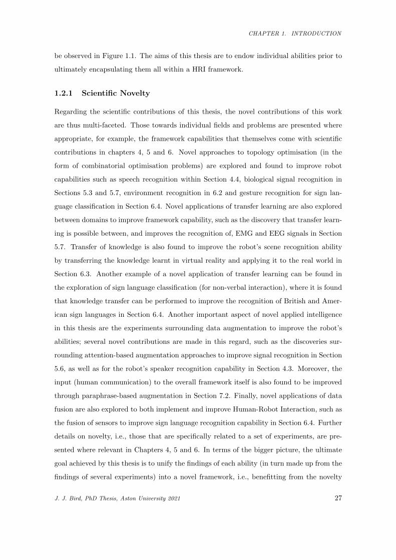
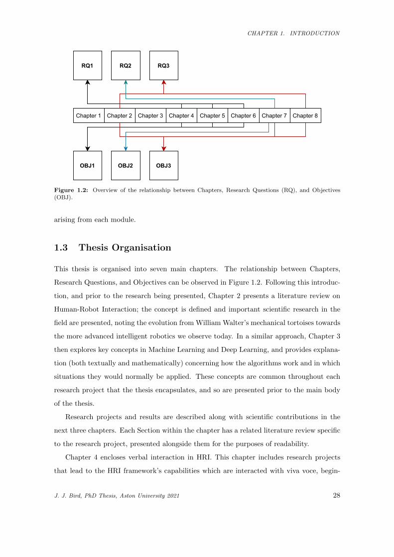
Figure 1.2: Overview of the relationship between Chapters, Research Questions (RQ), and Objectives(OBJ).
arising from each module.
1.3 Thesis Organisation
This thesis is organised into seven main chapters. The relationship between Chapters,
Research Questions, and Objectives can be observed in Figure 1.2. Following this introduc-
tion, and prior to the research being presented, Chapter 2 presents a literature review on
Human-Robot Interaction; the concept is defined and important scientific research in the
field are presented, noting the evolution from William Walter’s mechanical tortoises towards
the more advanced intelligent robotics we observe today. In a similar approach, Chapter 3
then explores key concepts in Machine Learning and Deep Learning, and provides explana-
tion (both textually and mathematically) concerning how the algorithms work and in which
situations they would normally be applied. These concepts are common throughout each
research project that the thesis encapsulates, and so are presented prior to the main body
of the thesis.
Research projects and results are described along with scientific contributions in the
next three chapters. Each Section within the chapter has a related literature review specific
to the research project, presented alongside them for the purposes of readability.
Chapter 4 encloses verbal interaction in HRI. This chapter includes research projects
that lead to the HRI framework’s capabilities which are interacted with viva voce, begin-
J. J. Bird, PhD Thesis, Aston University 2021 28
CHAPTER 1. INTRODUCTION
ning with an explanation of how audio data can be translated into a numerical dataset
containing statistical features (such as Mel-Frequency Cepstral Coefficients). The main
body of this chapter is made up of research projects that classify speech into phonemes
via evolutionary algorithms and deep learning, classification of a speaker’s sentiments and
accent, and recognition of the speaker as an individual entity. Moreover, within this chap-
ter, speaker recognition algorithms are improved through synthetic data augmentation by
both temporal and transformer methods. Chapter 5 similarly presents non-verbal interac-
tions in HRI, where experiments lead to HRI framework abilities that are interacted with
via other means than spoken voice. Several of the works consider biological signals as in-
put (i.e., brainwave and electromuscular activity), and so, this chapter provides an overall
background on biosignal processing, concerning how biological signals can be translated
into a non-temporal numerical vector describing electrical behaviour within a time window.
Following this, research projects are presented on HRI via biological signals. In addition
to the approaches, improvements to algorithms are explored through transfer learning and
synthetic data augmentation.
Following both verbal and non-verbal modes of interaction, Chapter 6 then presents
research into multi-modality interaction in HRI. These are abilities that the framework has
which require multiple modes of input data to an algorithm, similarly to how a human being
may use both vision and hearing to engineer a logical conclusion from a certain situation.
Capabilities such as multimodal scene recognition via consideration of vision and sound, and
sign language recognition via consideration of vision and 3D pose data are endowed within
the framework. Each algorithm is compared to the single-modal counterpart to discern how
much of an improvement multimodality may provide. Similarly to the prior two chapters,
abilities are improved by exploring concepts such as transfer learning.
Then, integration of findings and technologies are performed in Chapter 7. Within this
Chapter, the works performed during PhD studies form more than a sum of their parts
through a framework approach; the framework is presented and use cases are explored. The
contributions are finally discussed in the concluding chapters. Chapter 8 addresses the open
issues that were noted during literature review and discusses them with the framework in
mind. This chapter also finally concludes the thesis where research questions are revisited,
limitations and possible future works are noted, and final remarks are made.
J. J. Bird, PhD Thesis, Aston University 2021 29
CHAPTER 2. HUMAN-ROBOT INTERACTION
Chapter 2
Human-Robot Interaction
2.1 Introduction
Human-Robot Interaction (HRI) is the study of the interaction as well as the acceptance of
interaction between man and machine [11]. More specifically, Nouvelle AI robots, which,
rather than simply being computers that can locomote, instead respond and react accord-
ingly to their environment [12]. Nouvelle AI is an interesting and related concept of this
thesis, since a key hypothesis is that intelligence is an organic emergence from simple in-
teractions with the real world leading to further learning (similarly to how an infant child
learns from the world), rather than the opposing symbolic argument wherein all information
must be programmed [13]. This description can be attributed to Alan Turing’s ’situated
approach’ to AI [4, 14] whereby it was argued that a machine equipped with the best sensors
available could be taught to speak English by following ”the normal teaching of a child”.
To give a more recent example, MIT’s Cog aims to follow Turing’s theory by developing
intelligence through experience [15]. Several of the algorithms in the framework presented
by this thesis have multiple methods of improvement available via the collection of obser-
vations of different experiences, and exploring the possibility of improving the machine’s
intelligence through approaches such as transfer learning and synthetic data augmentation.
Social HRI is the ability for humans and robots to socially interact with one another
wherein, naturally, social interaction plays a specific key role for the robot[16, 17], with
Human-centred HRI being a system concerned with achieving tasks in an acceptable manner
according to a human, and Robot cognition-centred HRI being an intelligent system that
must learn to solve problems either alone or with limited direction [18]. Limited direction
J. J. Bird, PhD Thesis, Aston University 2021 30
CHAPTER 2. HUMAN-ROBOT INTERACTION
is useful, since it allows for a command “Robot do Task X”, which is deliberated by the
robot with “How do I do X? Then, do X”. To give a more specific example that appears
later on in this thesis, a human says to the robot “Look around and see if you can tell me
where you are.”, to which, the robot deliberates using a transformer-based natural language
classification algorithm which produces the classification of the task of Scene Recognition.
The robot then activates the camera and microphone to perform multi-modality scene
recognition and produces a response, e.g. “I am in the forest.”. Thus, the limited direction
of a human in the form of social interaction is then processed and performed through a
multi-step deliberation and actuation process. HRI in a social context has been noted to be
of growing importance in the applications of psychology and sociology in care. For example,
social robotics has been successful in aiding children with autism an all-important stepping
stone to developing social skills [19]. Social robotics has also been successfully trialled in
geriatric physiotherapy rehabilitation [20], and as a preventative measure for loneliness in
the elderly community [21]. Dar and Bernadet [22] suggest that the quality of Human-
to-Agent Interaction may have rapidly increased yet still remains a shadow of human-
to-human interaction. The authors note that increasing the number of communication
channels (in particular, proxemic and physiological channels of interaction) can lead to
higher resolution communication in the physical domain, and thus further the quality of
natural communication. The article argues that incorporation of implicit interaction would
lead to an alleviation of some of the open issues in interaction with non-human agents. Dar
and Bernadet also describe the process of purpose-based interaction, noting that interaction
should be achieved with minimal resources (e.g., effort and time) to be deemed satisfactory.
Humans communicate with machines differently than other humans, an example within the
aforementioned study being to speak slower and precisely during interaction; one of the
open issues that the work in this thesis aims to alleviate is to improve natural interaction
between human and machine.
Although this thesis explored some initial examples from history within the introduction,
the first experiments on emergent behaviours in robotics occurred in the 1940’s, wherein
William Walter’s ‘robot tortoises’ could autonomously follow light [23]. The intelligent
emergent behaviour was attained via a valve system that would either turn the robot if
light was not detected, or drive the robot towards the light if it was. The three parts,
a light sensor, valve system for turning, and the valve system for driving forwards, could
J. J. Bird, PhD Thesis, Aston University 2021 31
CHAPTER 2. HUMAN-ROBOT INTERACTION
not have exhibited this behaviour alone, and thus formed more than a sum of their parts
to complete the task. This work ultimately leads us to intelligent robotics, wherein the
consideration of multiple algorithms enables a growing exhibition of increasingly complex
behaviours, this concept is covered by the remainder of this chapter.
2.2 Emergence of Robotic Behaviour
Duffy noted that modern robot interaction, specifically in a social sense, is to engage in
meaningful and useful social interaction that inherently requires a degree of human-like
quality [24]. Interestingly, the work notes that imperfection is not actually a negative trait,
robots who are seemingly too intelligent can seem prone to weakness. It is important to
note that human interaction is not perfect. Within this impactful work, there is a point
made with high importance to this thesis; a social robot acts as an interfacing layer between
humans and technology, aiming to break down the barriers between digital information and
human beings. One of the goals of the framework in this thesis is just that, to enable
the accessibility of AI-based technologies through a socially interactive framework. In [25],
researchers presented a five-step approach for the classification of social robots: (i) Form,
from abstract to anthropomorphic, (ii) Modality, from unimodal to multimodal, (iii) Social
norms, from no knowledge to full knowledge of social norms, (iv) Autonomy, from no
autonomy whatsoever to a fully autonomous robot, and (v) interactivity ranging from no to
fully causal behaviours. The framework in this thesis aims to provide a software framework
compatible with any platform (to abide by a guideline set out below), and thus form is of less
importance than the other four classifications. Modality depends on the problem at hand,
since some problems may only require one type of sensor but it was noted that the solution
can be improved via late fusion of multiple data sources. Social norms are attained through
paraphrasing transformation of speech to better understand the message or request that the
user is trying to get across. Autonomy is limited outside of Duffy’s aforementioned goal of
breaking down barriers between man and technology, thus autonomy focuses on attaining
this goal. Interactivity, in this framework defined as the machine having the potential to
respond by reaction to an interaction, is relatively high in the presented framework given
that one of the goals is to enable access to technology through social interaction by a service
request.
J. J. Bird, PhD Thesis, Aston University 2021 32
CHAPTER 2. HUMAN-ROBOT INTERACTION
In 2006, Gorostiza et al. presented an automatic-deliberated architecture for social
human-robot interaction [26]. The framework is modular, for example, a chatbot platform
which takes input via the microphone and passes the parsed text to the deliberative layer,
which in turn generates an appropriate response and passes this back to the automatic level
in the form of an execution order. The execution order is then enacted with an actuator, in
this example, a text-to-speech unit which uses an artificial voice to say the text within the
execution order. The skills within this framework are greetings, face recognition, dialogue,
audiovisual interaction, non-verbal visual expressions, as well as dancing. The work thus
presented a multimodal interaction framework, noted by the authors that interaction was
more than merely a toy or tool. Glas et al. present a similar architecture with the specific
goals in mind of customer interaction in public [27]. In this example, service robots use
skills such as customer information, environmental information, and robot information to
perform socially interactive customer support.
One of the issues in Human-Robot Interaction is the range of components and scalability
of cognitive architectures. In 2018, Fischer et al. attempted to alleviate some of these issues
following the presentation of the iCub-HRI framework [28]. The framework provides the
abilities of entity recognition, tracking, speech recognition, motor actions, speech synthesis,
and joint attention for the iCub humanoid robot [29]. The framework follows a world-
self-action approach in somatic, reactive, adaptive, and contextual contexts; the world is
perceived, goals are considered, and actions are taken to achieve said goals within the world
environment. There are two main differences between the framework presented in this
thesis and the iCub-HRI framework. Firstly, the framework finally presented by this thesis
is platform agnostic, that is, the framework could be implemented on the iCub robot, but
could also be implemented on other robots that support the libraries used. For example, the
HRI framework presented by this thesis could be applied to any platform which supports
Python, TensorFlow, and Scikit Learn. The second main difference between the iCub-HRI
framework and the one engineered within this thesis, is that the work in this thesis also
deals with model improvement through transfer learning and data augmentation. The goal
of this module is to improve the robot’s learning abilities over time through the transfer of
knowledge from other data, or to learn from entirely synthetically generated data.
J. J. Bird, PhD Thesis, Aston University 2021 33
CHAPTER 2. HUMAN-ROBOT INTERACTION
2.3 Open Issues in HRI
Given the social nature of HRI, notable open issues in the field are often noticed by observa-
tion and conveyed through guidelines and rules for future researchers to interpret for their
specific goals in mind, and abide by in order to begin to solve issues that frameworks often
face. When presenting the aforementioned iCub-HRI framework based on much previous
research, Fischer et al. [28] presented five guidelines that HRI research should aim to follow.
Those guidelines are as follows:
• Adaptability and ease of use - adaption to related problems and robotic devices should
be easy to implement. Cross-dependency should be minimal to enable substitution.
• Provision of the overall framework - the provided framework should work as is and as
such provide useful routines and goals.
• Extendibility - integration of new technologies should be easy to implement with the
introduction of new modules. Software must be designed to expect and support new
modules.
• Shared and centralised knowledge representation - each module of the system should
have access to the same sources of data and knowledge.
• Open software - code should be open source and available to researchers
An interesting observation here is on the point of extendibility. The iCub-HRI paper was
authored by ten researchers, and generally contains around eight abilities or categories of
abilities (noted in Section 2.1). Frameworks are thus required to be extendible and scalable
given that a HRI ability tends to be an entire field of applied intelligence in itself, with
differing requirements in terms of the fields of study of the researchers involved. It is for the
same reason that this thesis presents a general suite of abilities which include verbal com-
munication, specifically, speech recognition (phonetic sounds and accent), speech synthesis,
and sentiment analysis. The framework also presents non-verbal and multimodal abilities
including biological signal classification (EEG and EMG), sign language recognition, and
scene recognition. The framework is designed to be easily extended with further abilities in
the future, and the aforementioned general range of abilities are explored and implemented
to provide enough for interaction with the robots. Generally, albeit often focusing moreso
J. J. Bird, PhD Thesis, Aston University 2021 34
CHAPTER 2. HUMAN-ROBOT INTERACTION
on physical robotic behaviours such as navigation, most works concerning design of HRI
frameworks encapsulate the above five points [30, 31, 32]. Specifically, in Drury et al. [32],
the authors noted that they observed “major problems” in the field that could be remedied
by attention to the following guidelines:
• Enhancement of awareness - this guideline, as previously noted, focuses moreso on
physical robotic behaviour. An enhancement of awareness, as described in the afore-
mentioned paper, deals with providing a map of where the robot has been and provides
more environmental information to the robot for the benefit of operator awareness.
• Lowering of cognitive load - the operator should not need to mentally fuse modes of
data, rather, the framework itself should provide fused information.
• Increase of efficiency - provide an interface that supports multiple robots within a
single window, and to minimise the use of multiple windows where feasible.
• Provide help - the user of the framework should be aided in the selection of robotic
autonomy and modality.
This thesis considers an enhancement of awareness in terms of single and multi-modality
environment recognition rather than for navigation. Although this differs slightly from
Drury et al.’s description, it still provides the benefit of improved operator awareness by
allowing the robot to autonomously recognise surroundings. Given the importance of the
above guidelines and related works, they are later revisited in the concluding sections of
this thesis (Chapter 8) during the discussion of the framework produced and the scientific
contributions that it thus makes.
2.4 Phonetic Speech Recognition
Phonology is the study of the fundamental components of a spoken language as well as their
relationship with one another [33]. When the English language is considered, spelling does
not consistently represent the sound of language, for example: (i) the same sound may be
represented by many letters or a combination of letters (e.g. he and people); (ii) the same
letter may represent a variety of sounds (e.g. father and many); (iii) a combination of letters
may represent a single sound (e.g. shoot and character); (iv) a single letter may represent
J. J. Bird, PhD Thesis, Aston University 2021 35
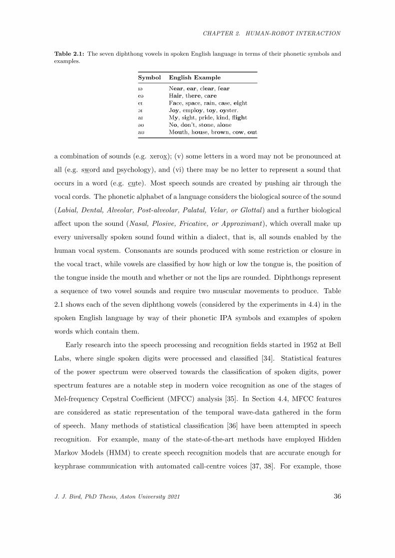
CHAPTER 2. HUMAN-ROBOT INTERACTION
Table 2.1: The seven diphthong vowels in spoken English language in terms of their phonetic symbols andexamples.
Symbol English Example
I@ Near, ear, clear, feare@ Hair, there, careeI Face, space, rain, case, eightOI Joy, employ, toy, oyster.aI My, sight, pride, kind, flight@U No, don’t, stone, aloneaU Mouth, house, brown, cow, out
a combination of sounds (e.g. xerox); (v) some letters in a word may not be pronounced at
all (e.g. sword and psychology), and (vi) there may be no letter to represent a sound that
occurs in a word (e.g. cute). Most speech sounds are created by pushing air through the
vocal cords. The phonetic alphabet of a language considers the biological source of the sound
(Labial, Dental, Alveolar, Post-alveolar, Palatal, Velar, or Glottal) and a further biological
affect upon the sound (Nasal, Plosive, Fricative, or Approximant), which overall make up
every universally spoken sound found within a dialect, that is, all sounds enabled by the
human vocal system. Consonants are sounds produced with some restriction or closure in
the vocal tract, while vowels are classified by how high or low the tongue is, the position of
the tongue inside the mouth and whether or not the lips are rounded. Diphthongs represent
a sequence of two vowel sounds and require two muscular movements to produce. Table
2.1 shows each of the seven diphthong vowels (considered by the experiments in 4.4) in the
spoken English language by way of their phonetic IPA symbols and examples of spoken
words which contain them.
Early research into the speech processing and recognition fields started in 1952 at Bell
Labs, where single spoken digits were processed and classified [34]. Statistical features
of the power spectrum were observed towards the classification of spoken digits, power
spectrum features are a notable step in modern voice recognition as one of the stages of
Mel-frequency Cepstral Coefficient (MFCC) analysis [35]. In Section 4.4, MFCC features
are considered as static representation of the temporal wave-data gathered in the form
of speech. Many methods of statistical classification [36] have been attempted in speech
recognition. For example, many of the state-of-the-art methods have employed Hidden
Markov Models (HMM) to create speech recognition models that are accurate enough for
keyphrase communication with automated call-centre voices [37, 38]. For example, those
J. J. Bird, PhD Thesis, Aston University 2021 36
CHAPTER 2. HUMAN-ROBOT INTERACTION
used when calling a bank to direct a customer’s call to the correct department. Researchers
noted that the success achieved was case-specific and that complex applications of the
HMM for transcription of speech to text may not experience the same level of success. A
related study found that Similar Pattern Analysis (SPA) could classify a very limited set
of sounds with 90% accuracy [39], also noting the application in the domain of human-
machine interaction in terms of aiding children with temporal processing disorders who
have difficulty discerning sounds produced in a short time frame, i.e., those that occur
often in natural speech. Research focusing on the classification of acoustic events such as
keywords in speech achieved 80.79% accuracy using a Random Forest of decision trees [40].
A similar approach was employed with an accuracy of 81.5% for a set of 14 sound effects [41],
although it is worth noting that the acoustic events in the last aforementioned study were
not produced by humans. A particularly powerful method of machine learning approach
for speech recognition, Connectionist Speech Recognition, was noted to be an ensemble
fusion of predictions between a Multilayer Perceptron (MLP) and a Hidden Markov Model
due to their largely statistical differences in prediction and yet high accuracies in terms of
classifying audio data [42]. A more recent work found that generalisation between language
is difficult in [43]; noting the scarcity of data available for Lithuanian speech recognition
systems, researchers found high classification ability of spoken Lithuanian phonetics via a
sequence-to-sequence approach through encoder-decoder models, achieving +99% over 10-
fold cross-validation. A related benchmarking study of the Random Forest classifier found
that language based speech recognition became most optimal, and accurate, at a forest of 50
random decision trees all voting by average probability in a simple ensemble, the error rate of
the multi-language corpus data for classification was found to be a relatively low 13.4% [44].
The Random Forest classification method was also used in classifier feature selection, from a
dataset of acoustic audio features, to select an apt set of attributes for emotion classification
from spoken audio data at approximately 70% accuracy over all test subject sets (who
were divided by gender) [45]. US-based systems such as DARPAs EARS program and
IARPA Babel operate a method of speech recognition with the extra step of specific-goal
keyword segmentation and isolation (a cost-based machine learning approach), which are
then used for security purposes by the National Security Agency (NSA) to autonomously
detect high-risk organisations via a computer system rather than the classical method of
human wiretapping [46].
J. J. Bird, PhD Thesis, Aston University 2021 37
CHAPTER 2. HUMAN-ROBOT INTERACTION
Limited work on phoneme-based voice recognition has been performed. A bidirectional
Long Short-term Memory neural network was tuned to an accuracy of 87.7% [47] on a
dataset of phonetic sounds. It is worth noting the usefulness of temporal-considerate ma-
chine learning techniques (inputs as batches/streams of data vectors). A limited dataset
of the sounds “B”, “D”, and “G” was classified with an overall accuracy of 99.1% using
a Time Delayed Neural Network, outperforming a Hidden Markov Model by 1.9% [48].
This study suggests the promising capabilities of a temporal-considerate neural network for
speech recognition. However, the study was performed on a limited dataset that was not
an accurate reflection of the multitude of phonemes found in human language, specifically
in spoken English. A Deep Learning approach through the use of a Convolutional Neu-
ral Network (CNN) offers a preliminary solution to the spoken accent problem in speech
recognition [49]. The approach can derive a matrix which would be applied to the Mel-
Frequency Cepstral Coefficients (MFCC) of a sound which would effectively attempt to
mitigate differences in spoken accent by translating between them, with promising prelimi-
nary experiments resulting in success. It is observed that all of the related works made use
of temporal statistical analysis of soundwaves to create stationary data for classification,
rather than attempting to simply classify the continuous sound. Furthermore, the most
commonly observed method of generating this mathematical description is to analyse pat-
terns found in short-term Mel-Frequency Cepstral Coefficient (MFCC) data at 100-500ms.
It is also worth noting that a majority of the studies discussed here present results based on
train-test split of the data, which is prone to overfitting [50, 51] and thus fail to generalise
to unseen data (which is in itself the point of speech recognition). The study in Section 4.4
therefore performs 10-fold cross validation and presents the mean accuracy over the folds
as well as the standard deviation of the results to avoid overfitting and better model out-
of-sample data, which is important for generalisation and for a genetic search itself, since
an algorithm that simply searches for network hyperparameters that best over-fit the vali-
dation data is undesirable. Due to the temporal nature of speech, it is worth noting that a
Zoughi et al. [52] found success in performing an adaptive sliding window and Convolutional
Neural Network approach to various datasets including the TIMIT phoneme classification
dataset, where the window would adapt to the specific duration of the phonetic sound.
J. J. Bird, PhD Thesis, Aston University 2021 38
CHAPTER 2. HUMAN-ROBOT INTERACTION
2.5 Speaker Recognition and Synthesis
Verification of a speaker is the process of identifying a single individual from many others
by spoken audio data [53]. That is, the recognition of a set of the person’s speech data X
specifically from a speech set Y where X ∈ Y . In the simplest sense, this can be expressed
as a binary classification problem; for each data object o, is o ∈ X? Is the speaker to be
recognised speaking, or is it another individual? Speaker recognition is important for social
HRI [54] (the robot’s perception of the individual based on their acoustic utterances),
Biometrics [55], and Forensics [56] among many others. Researchers found the relative
ease of classifying 21 speakers from a limited set [57], but the problem becomes more
difficult as it becomes more realistic, where classifying a speaker based on their utterances
is increasingly difficult as the dataset grows [58, 59, 60]. In Section 4.3, the speaker is
recognised from many thousands of other examples of human speech from the Flickr8k
and Fluent Speech Commands speaker datasets. Data scarcity and its negative impact on
speech processing systems has been noted as an open issue in the current state of the art [58,
61, 62, 63]. Current suggestions to improve these issues include Deep Belief Networks [64]
and compression of utterances into i-vectors [65]. Thanks to their growing prominence,
generative models have been suggested as a potential solution to data scarcity within a
variety of fields [66, 67, 68]. The field of exploring augmented data to improve classification
algorithms is relatively young, but there exist several prominent works that show success in
applying this approach. When augmented data from the SemEval dataset is learned by by
a Recurrent Neural Network (RNN), researchers found that the overall best F-1 score was
achieved for relation classification in comparison to the model learning only from the dataset
itself [69]. A recent study also showed GANs may be able to aid in producing synthetic
data for speaker recognition [70]. Temporal models have been observed to be successful
in generating MFCC data [71], which is the data type considered in Section 4.3. Many
prominent works in speech recognition consider temporal learning to be essential [72, 73, 74]
and for generation of likewise temporal data [75, 71, 76]. If it is possible to generate data
that bares similarity to the real data, then it could improve the models, while also reducing
the need for large amounts of real data to be collected.
Tacotron is a Spectrogram Feature Prediction Deep Learning Network [77, 76] inspired
by the architecture of Recurrent Neural Networks (RNN) in the form of Long Short-term
J. J. Bird, PhD Thesis, Aston University 2021 39
CHAPTER 2. HUMAN-ROBOT INTERACTION
Memory (LSTM). The Tacotron model uses character embedding to represent a text, as
well as the spectrogram of the audio wave. Recurrent architectures are utilised due to their
ability of temporal awareness, since speech is a temporal activity [74, 78]. That is, where
frame n does not occur at the start or end of the wave, it is directly influenced and thus has
predictive ability both to and for frames n−1 and n+1. Since audio may possibly be lengthy,
a nature in which recurrence tends to fail, ‘attention’ is modelled to allow for long sequences
in temporal learning and as such its representation [79]. Actual speech synthesis, the
translation of spectrograms to audio data, is performed via the Griffin-Lim algorithm [80].
This algorithm performs the task of signal estimation via its Short-time Fourier Transform
(STFT) by iteratively minimising the Mean Squared Error (MSE) between estimated STFT
and modified STFT. STFT is a Fourier-transform in which the sinusoidal frequency of the
content of local sections of a signal are determined [81]. Alternate notations of English
through encoding and flagging have been shown to provide more understanding of various
speech artefacts. A recent work by researchers at Google found that spoken prosody could
be produced [82]. The work’s notation allowed for the patterns of stress and intonation in
a language. The implementation of a Wave Network [83] has shown to produce similarity
gains of 50% when use in addition to the Tacotron architecture.
2.6 Accent Recognition
Hidden Markov Models (HMM), since their inception in 1966, remain a modern approach
for speech recognition due to their retaining of effectiveness given more computational
resources. An earlier work from 1996 found that, using 5 hidden Markov states due to the
computational resources available at the time, four spoken accents could be classified at
an observed accuracy of 74.5%[84]. It must be noted that deeper exploration into optimal
HMM topology and structure is now possible due to the larger degree of processing power
available to researchers in the modern day. A more modern work found that Support
Vector Machines (SVM) and HMM could classify between three different national locales
(Chinese, Indian, Canadian) at an average accuracy of 93.8% for both models [85], though,
this study only classified data from male speakers due to the statistical frequency differences
between gender and voice. Long Short Term Memory neural networks are often succesfully
experimented with in terms of accent recognition. A related experiment found accuracies
J. J. Bird, PhD Thesis, Aston University 2021 40
CHAPTER 2. HUMAN-ROBOT INTERACTION
at around 50% when classifying 12 different locales[86]. Of the dataset gathered from
multiple locations across the globe, it was observed that the highest recall rates were that
of Japanese, Chinese, and German scoring 65%, 61% and 60% respectively. Subjects were
recorded in their native language. An alternative network-based approach, Convolutional
Neural Networks, were used to classify speech from English, Korean and Chinese dialects
at an average accuracy of 88%[87]. A proposed approach to the accent problem in speech
recognition, also using a CNN, offered a preliminary study into deriving a conversion matrix
to be applied to Mel-frequency Cepstral Coefficients which would act to translate the user’s
accent into a specified second accent before speech recognition is performed[88].
In terms of open issues, many accent recognition experiments rarely define the spoken
language itself, often resulting in the classification of a subject speaking their native lan-
guage in their natural locale. Given this, it is therefore possible that classifiers would not
only learn from accent, but from natural language patterns as a form of audible Natural
Language Processing, since such effects are also represented within MFCC data. Towards
the goal of improving voice recognition for non-native English speakers who are speaking En-
glish, the previous models would be therefore questionable. Therefore the originality of the
experiments in Section 4.5 is to classify data retrieved from native and non-native English
speakers (who are all requested to pronounce sounds from the English phonetic dictionary,
as if they were speaking in English), with the ultimate goal of providing a path to improving
voice recognition on English language devices and services for non-native speakers.
2.6.0.1 Acoustic Fingerprint
Acoustic Fingerprinting is the process of producing a summary of an audio signal to identify
or locate similar samples of audio data [89]. To produce similarity, alignment of audio is per-
formed and subsequently the two time-frequency graphs (spectrograms) have the distance
between their statistical properties such as peaks measured. This process is performed to
produce a percentage similarity between a pair of audio clips.
Fingerprint similarity measures allow for the identification of data from a large library,
the algorithm operated by the music search engine Shazam allows for the detection of a song
from a database of many millions [90]. Detection in many cases was succesfully performed
with only a few milliseconds of search data. Although this algorithm is often used for
J. J. Bird, PhD Thesis, Aston University 2021 41
CHAPTER 2. HUMAN-ROBOT INTERACTION
plagiarism detection and search engines within the music industry, the ability to spoof a
similarity would argue that the artificial data closely matches that of real data. This is
performed in this experiment by comparing the fingerprint similarities of audio produced
by a human versus the audio produced by the Griffin-Lim algorithm on the spectrographic
prediction of the Tacotron networks.
2.7 Sign Language Recognition
Sign Languhand trackingon (SLR) is a collaboration of multiple fields of research which
can involve pattern matching, computer vision, natural language processing, and linguis-
tics [91, 92, 93]. The core of SLR is oftentimes focused around feature engineering and
learning model-based approach to recognise hand-shapes [94]. Classically, SLR was usually
performed by temporal models trained on sequences of video. Many works from the late
1990’s through to the mid-2000’s found the best results when applying varying forms of
Hidden Markov Models (HMMs) to videos [95, 96, 97, 98], HMMs are predictive models of
transition (prior distribution) and emission probabilities (conditional distribution) of hid-
den states. To give a specific example, researchers found in [95] that hand-tracking via a
camera and classification of hand gestures while wearing solidly coloured gloves (similar to
chroma key) was superior to hand tracking without a glove. In this work, a vector of 8
features were extracted from the hands including 2-dimensional X, Y positions, the angle of
the axis with the least inertia, and the eccentricity of a bounding ellipse around the hand.
That is, four features for each hand. These vectors then provided features as input to the
HMM. More recently, given the affordable sensors that provide more useful information
than a video clip, studies have focused upon introducing this information towards stronger
and more robust real-time classification of non-verbal languages. Sign language recognition
with depth-sensing cameras such as Kinect and Leap Motion is an exciting area within the
field due to the possibility of accessing accurate 3D information from the hand through
stereoscopy similar to human depth perception via images from two eyeballs. Kinect allows
researchers to access RGBD channels via a single colour camera and a single infrared depth-
sensing camera. A Microsoft Kinect camera was used to gather data in [99], and features
were extracted using a Support Vector Machine from depth and motion profiles. Experi-
ments in [100] found that generating synchronised colour-coded joint distance topographic
J. J. Bird, PhD Thesis, Aston University 2021 42
CHAPTER 2. HUMAN-ROBOT INTERACTION
descriptor and joint angle topographical descriptor and used as input to a two-steam CNN
produced effective results; the CNNs in Section 6.4 are therefore concatenated by late fu-
sion similar to the multi-modality method in this study and results were around 92% for
a 20-class dataset. In terms of RGB classification specifically, many state of the art works
have argued in favour of the VGG16 architecture [101] for hand gesture recognition to-
wards sign language classification [102]. These works include British [103], American [104],
Brazilian [105] and Bengali [106] Sign Languages among others. Given the computational
complexity of multi-modality when visual methods are concerned in part, multi-modality is
a growing approach to hand gesture recognition. Researchers have shown that the approach
of fusing the LMC and flexible sensors attached to the hand via Kalman filtering [107] is
promising. Likewise, in this regard, recent work has also shown that RGBD (Realsense)
along with a physical sensor-endowed glove can also improve hand tracking algorithms [108].
Given the nature of SLR, physically-worn devices are an unrealistic expectation for users
to accept when real-world situations are considered, e.g. should someone wish to sign in
a hotel lobby for staff who do not know sign language. Due to this issue in the field, an
approach is followed in Section 6.4 of two nonphysical sensors that are placed in front of
the subject as a ‘terminal’. That is, facing towards a camera and Leap Motion sensor are
similar to natural social interaction and do not require the adoption of a physical device on
the body.
Transfer Learning is a relatively new idea applied to the field of Sign Language recogni-
tion. In [109], researchers found it promising that knowledge could be transferred between
large text corpora and BSL via both LSTM and MLP methods, given that sign language
data is often scarcely available. In the experiments in Section 6.4, rather than transferring
between syntax-annotated text corpora, the aim is instead to follow the multi-sensor experi-
ments with transfer learning between two different sign languages, i.e., transferring between
the same task but in two entirely different languages (British Sign Language and American
Sign Language). Features recorded from the 26 letters of the alphabet in American Sign
Language were observed to be classified at 79.83% accuracy by a Support Vector Machine
algorithm [110]. Similarly to the aforementioned work, researchers found that a different
dataset also consisting of 26 ASL letters were classifiable at 93.81% accuracy with a Deep
Neural Network [111]. Another example achieved 96.15% with a deep learning approach on
a limited set of 520 samples (20 per letter) [112]. Data fusion via Coupled Hidden Markov
J. J. Bird, PhD Thesis, Aston University 2021 43
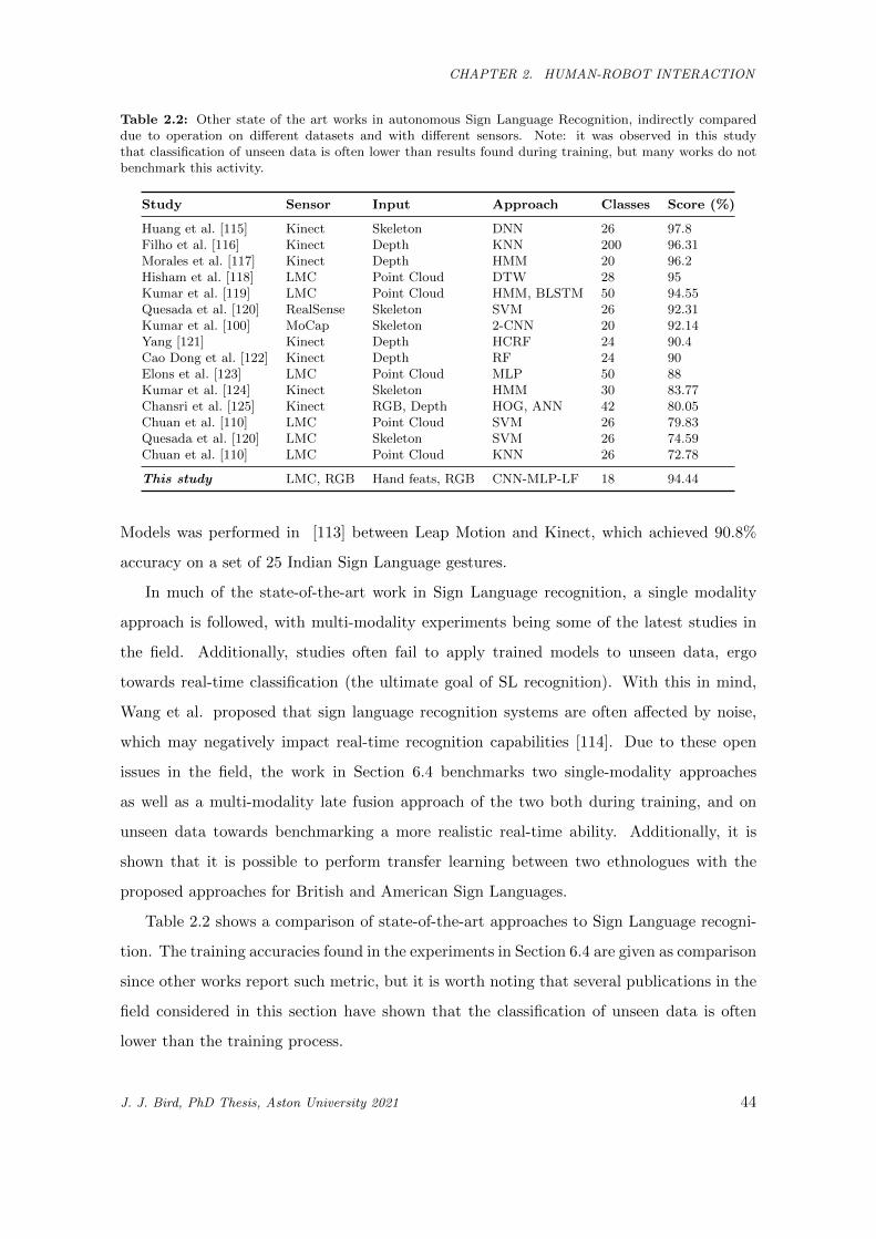
CHAPTER 2. HUMAN-ROBOT INTERACTION
Table 2.2: Other state of the art works in autonomous Sign Language Recognition, indirectly compareddue to operation on different datasets and with different sensors. Note: it was observed in this studythat classification of unseen data is often lower than results found during training, but many works do notbenchmark this activity.
Study Sensor Input Approach Classes Score (%)
Huang et al. [115] Kinect Skeleton DNN 26 97.8Filho et al. [116] Kinect Depth KNN 200 96.31Morales et al. [117] Kinect Depth HMM 20 96.2Hisham et al. [118] LMC Point Cloud DTW 28 95Kumar et al. [119] LMC Point Cloud HMM, BLSTM 50 94.55Quesada et al. [120] RealSense Skeleton SVM 26 92.31Kumar et al. [100] MoCap Skeleton 2-CNN 20 92.14Yang [121] Kinect Depth HCRF 24 90.4Cao Dong et al. [122] Kinect Depth RF 24 90Elons et al. [123] LMC Point Cloud MLP 50 88Kumar et al. [124] Kinect Skeleton HMM 30 83.77Chansri et al. [125] Kinect RGB, Depth HOG, ANN 42 80.05Chuan et al. [110] LMC Point Cloud SVM 26 79.83Quesada et al. [120] LMC Skeleton SVM 26 74.59Chuan et al. [110] LMC Point Cloud KNN 26 72.78
This study LMC, RGB Hand feats, RGB CNN-MLP-LF 18 94.44
Models was performed in [113] between Leap Motion and Kinect, which achieved 90.8%
accuracy on a set of 25 Indian Sign Language gestures.
In much of the state-of-the-art work in Sign Language recognition, a single modality
approach is followed, with multi-modality experiments being some of the latest studies in
the field. Additionally, studies often fail to apply trained models to unseen data, ergo
towards real-time classification (the ultimate goal of SL recognition). With this in mind,
Wang et al. proposed that sign language recognition systems are often affected by noise,
which may negatively impact real-time recognition capabilities [114]. Due to these open
issues in the field, the work in Section 6.4 benchmarks two single-modality approaches
as well as a multi-modality late fusion approach of the two both during training, and on
unseen data towards benchmarking a more realistic real-time ability. Additionally, it is
shown that it is possible to perform transfer learning between two ethnologues with the
proposed approaches for British and American Sign Languages.
Table 2.2 shows a comparison of state-of-the-art approaches to Sign Language recogni-
tion. The training accuracies found in the experiments in Section 6.4 are given as comparison
since other works report such metric, but it is worth noting that several publications in the
field considered in this section have shown that the classification of unseen data is often
lower than the training process.
J. J. Bird, PhD Thesis, Aston University 2021 44
CHAPTER 2. HUMAN-ROBOT INTERACTION
2.8 Sentiment Analysis
Sentiment analysis, or opinion mining, is the study of deriving opinions, sentiments, and
attitudes from lingual data such as speech, actions, behaviours, or written text. Sentiment
Classification is an approach that can class this data into nominal labels (eg. ‘this re-
mark has a negative valence’ ) or continuous polarities or score which map to their overall
sentiment. With the rise of online social media, extensive amounts of opinionated data
are available online, which can be used in classification experiments which require large
datasets. Negative polarity was used to analyse TripAdvisor reviews [126] on a scale of
negative-neutral-positive, the findings show that each review rating of one to five stars each
has unique distributions of negative polarity. This unique pattern suggests the possibility
of further extending the two-polarity three-sentiment system to a further five levels. A sim-
ilar three-class sentiment analysis was successfully trained on Twitter data [127]. Another
related work with Twitter Sentiment Analysis found that hashtags and emoticons/emoji
were effective additional attributes to improve classifiers [128]. Exploration of TripAdvi-
sor reviews found that separation via root terms, ‘food’, ‘service’, ‘ambiance’ and ‘price’
provided a slight improvement for machine learning classification [129].
With increasing availability of computing resources for lower costs, accurate classifi-
cation is enabled on increasingly larger datasets over time, giving rise to cross-domain
applications through more fine-tuned rules and complex patterns of attribute values. That
is, a model trained on dataset A can be used to classify dataset B. This has been effec-
tively shown through multiple-source data to produce an attribute thesaurus of sentiment
attributes [130]. Researchers also found that rule-based classification of large datasets are
unsuited to cross-domain applications, but machine-learning techniques on the same data
shows promising results [131].
Observing the results of the related studies on social media sentiment analysis (Twitter,
TripAdvisor, IMDB, etc.) shows a prominence of three-level sentiment classification, with
only one class for negative and one for positive along with a neutral class, with an overall
result being calculated with derived polarities. With the large amount of data available
correlating to a user’s specification of class outside of this range of three, the work in
Section 4.7 suggests a more extensive sentiment classification paradigm to co-ordinate with
user’s review scores, to better use human-sourced data. The end goal thus is to engineer
J. J. Bird, PhD Thesis, Aston University 2021 45
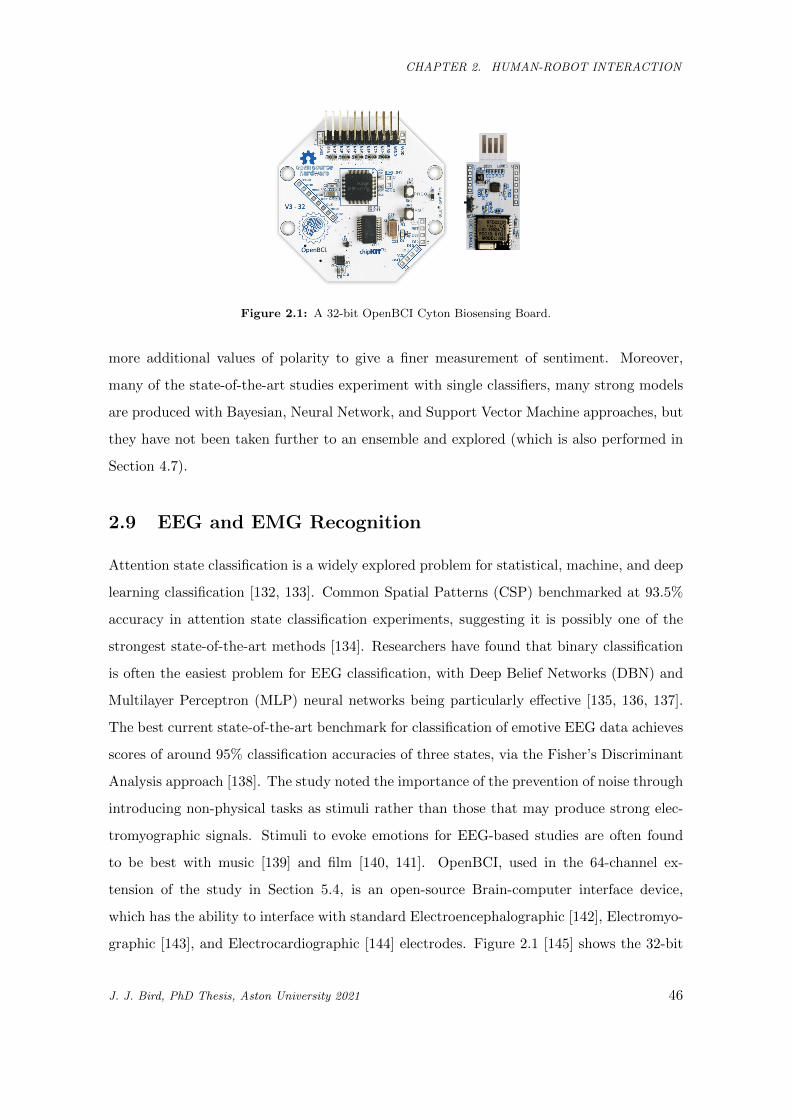
CHAPTER 2. HUMAN-ROBOT INTERACTION
Figure 2.1: A 32-bit OpenBCI Cyton Biosensing Board.
more additional values of polarity to give a finer measurement of sentiment. Moreover,
many of the state-of-the-art studies experiment with single classifiers, many strong models
are produced with Bayesian, Neural Network, and Support Vector Machine approaches, but
they have not been taken further to an ensemble and explored (which is also performed in
Section 4.7).
2.9 EEG and EMG Recognition
Attention state classification is a widely explored problem for statistical, machine, and deep
learning classification [132, 133]. Common Spatial Patterns (CSP) benchmarked at 93.5%
accuracy in attention state classification experiments, suggesting it is possibly one of the
strongest state-of-the-art methods [134]. Researchers have found that binary classification
is often the easiest problem for EEG classification, with Deep Belief Networks (DBN) and
Multilayer Perceptron (MLP) neural networks being particularly effective [135, 136, 137].
The best current state-of-the-art benchmark for classification of emotive EEG data achieves
scores of around 95% classification accuracies of three states, via the Fisher’s Discriminant
Analysis approach [138]. The study noted the importance of the prevention of noise through
introducing non-physical tasks as stimuli rather than those that may produce strong elec-
tromyographic signals. Stimuli to evoke emotions for EEG-based studies are often found
to be best with music [139] and film [140, 141]. OpenBCI, used in the 64-channel ex-
tension of the study in Section 5.4, is an open-source Brain-computer interface device,
which has the ability to interface with standard Electroencephalographic [142], Electromyo-
graphic [143], and Electrocardiographic [144] electrodes. Figure 2.1 [145] shows the 32-bit
J. J. Bird, PhD Thesis, Aston University 2021 46
CHAPTER 2. HUMAN-ROBOT INTERACTION
Arduino-compatible board for biosensing. OpenBCI with selected electrodes has seen 95%
classification accuracies of sleep states when discriminative features are considered by a Ran-
dom Forest model in the end-to-end system Light-weight In-ear BioSensing (LIBS) [146]. In
Section 5.4, OpenBCI data is used to detect eye state, that is, whether or not the subject has
opened or closed their eyes. In addition to the obvious nature of muscular activity around
the eyes, according to Brodmann’s Areas, the visual cortex is also an indicator of visual
stimuli [147, 148], and thus a higher resolution EEG is recommended for full detection. In
[149], researchers achieved an accuracy of 81.2% of the aforementioned states through a
Gaussian Support Vector Machine trained on data acquired from 14 EEG electrodes. It
was suggested that with this high accuracy, the system could be potentially used in the
automatic switching of autonomous vehicle states from manual driving to autonomous, in
order to prevent a fatigue-related accident. Another related work found that K-Star clus-
tering enabled much higher classification accuracies of these states to around 97% [150],
but it must be noted that only one subject was considered and thus generalisation and
further use beyond the subject would be considered difficult when generalisation works are
considered [151, 152]; in this study, ten subjects are considered. In a similar dataset as seen
in this work, researchers found that K-Nearest Neighbour classification (where k = 3) could
produce a classification accuracy of 84.05% [153]. In the classification problem of the states
of eyes open and closed (a binary classification problem), a recent work found that statisti-
cal classification via 7-nearest neighbours of the data following temporal feature extraction
achieved a mean accuracy of 77.92%[154]. The study extracted thirteen temporal features
and found that wave kurtosis was a strong indicator for the autonomous inference of the
two states.
In terms of the related work to the EMG experiments in Section 5.5. the discrimination
of affirmative and negative responses in the form of thumbs up and thumbs down was shown
to be possible in a related study [155], within which the two actions were part of a larger
eight-class dataset which achieved 87.6% on average for four individual subjects. Linear
Discriminant Analysis (LDA) was used to classify features generated by a sliding window
of 200ms in size with a 50ms overlap technique similar to that followed in this work; the
features were mean absolute value, waveform length, zero crossing and sign slope change
for the EMG itself and mean value and standard deviation observed by the accelerometer.
In [156], researchers followed a similar process of classification of minute thumb movements
J. J. Bird, PhD Thesis, Aston University 2021 47
CHAPTER 2. HUMAN-ROBOT INTERACTION
when using an Android mobile phone. Results showed that accuracies of 89.2% and 82.9%
are achieved for a subject holding a phone and not holding a phone respectively when two
seconds of EMG data is classified with a K-Nearest Neighbour (KNN) classification algo-
rithm. A more recent work explored the preliminary applications of image enhancement
to surface electromyographs showing their potential to improve the classification of muscle
characteristics[157]. Calibrations in the related works, where performed, are through the
process of Inductive Transfer Learning (ITL) and Supervised Transductive Transfer Learn-
ing (STTL). According to [158] and [159], ITL is the process satisfied when the source
domain labels are available as well as the target labels, this is leveraged in the calibration
stage, in which the gesture being performed is known. STTL is the process in which the
source domain labels are available but the target is not, this is the validation stage in this
study, when a calibrated model is benchmarked on further unknown data during the appli-
cation of a calibrated model. Transfer learning is the process of knowledge transfer from one
learned task to another [160], experiments in Section 5.5 found it difficult to generalise a
model to new subjects and thus the application of a model to new data is considered a task to
be solved by transfer learning; transfer learning often shows strong results in the application
of gesture classification in related state-of-the-art works [161, 162, 163, 164, 165]. Often-
times in the related literature, only one method of Machine Learning is applied, and thus
different statistical techniques are rarely compared as benchmarks on the same dataset.
In Section 5.5, many statistical techniques of feature selection and machine learning are
applied to explore the abilities of each in EMG classification. Very little exploration of
generalisation has been performed, researchers usually opt to present classification ability
of a dataset and there is a distinct lack of exploration when unseen subjects are concerned.
This is important for real-world application. Therefore, in Section 5.5, models attempt to
classify data gathered from new subjects and experience failure. This is further remedied by
the suggestion of a short calibration task, in which the generalisaton then succeeds through
the process of inductive transfer learning and transductive transfer learning.
2.10 Biosignal Augmentation and Transfer
Previous work has demonstrated the benefits of augmenting biological signal datasets to im-
prove the classification results. The majority of such research makes use of simple techniques
J. J. Bird, PhD Thesis, Aston University 2021 48
CHAPTER 2. HUMAN-ROBOT INTERACTION
to overcome the common issues of data scarcity and calibration time. A common approach is
to generate synthetic signals by re-arranging components of real data. Lotte [166] proposed
a method of “Artificial Trial Generation Based on Analogy” where three data examples
x1, x2, x3 provide examples and an artificial xsynthetic is formed which is to x3 what x2 is to
x1. A transformation is applied to x1 to make it more similar to x2, the same transformation
is then applied to x3 which generates xsynthetic1. This approach was shown to improve the
performance of a Linear Discriminant Analysis classifier on three different datasets. Dai et
al. [167] performed similar rearrangements of waveform components in both the time and
frequency domains to add three times the amount of initially collected EEG data, finding
that this approach could improve the classification accuracy of a Hybrid Scale Convolutional
Neural Network. This work showed that data augmentation allowed the model to improve
the classification of data for individual subjects that were specifically challenging in terms
of model’s classification ability. Dinares-Ferran [168], and subsequently Zhang [169] decom-
posed EEG signals into Intrinsic Mode Functions and constructed synthetic data frames by
arranging these IMFs into new combinations, demonstrating improvements of the classifi-
cation performance of motor imagery-based BCIs while including these new signals. Other
researchers have proposed data augmentation techniques commonly used in other domains
such as image classification techniques with positive results. As an example Shovon et
al. [170] applied conventional image augmentation techniques (such as altering the rotation,
zoom, and brightness [171]) to spectral images formed from EEG analysis to increase the
size of a public EEG dataset, which ultimately led to improved classification accuracy when
compared to related state-of-the-art works utilising the same dataset. Most state-of-the-art
research in biological signal augmentation shows great impact can be derived from relatively
simple techniques. For example, both Freer [172] and Wang [173] observed that introducing
noise into gathered data to form additional data points improved the learning ability of
several models, which otherwise performed relatively poorly. Tsinganos et al. [174] studied
the approaches of magnitude warping, wavelet decomposition, and synthetic surface EMG
models (generative approaches) for hand gesture recognition, finding classification perfor-
mance increases of up to +16% when augmented data was introduced during training. More
recently, data augmentation studies have begun to focus on the field of deep learning, more
specifically on the ability of generative models to create artificial data which is then intro-
1Equations for Lotte’s EEG generation technique can be found in [166]
J. J. Bird, PhD Thesis, Aston University 2021 49
CHAPTER 2. HUMAN-ROBOT INTERACTION
duced during the classification model training process. In 2018, Luo et al. [175] observed
that useful EEG signal data could be generated by Conditional Wasserstein Generative
Adversarial Networks (GANs), which was then introduced to the training set in a classi-
cal train-test learning framework. The authors found the classification performance was
improved when such techniques were introduced. Likewise, Zhang and Liu [176] applied
similar Deep Convolutional GANs (DC-GAN) to EEG signals given that training examples
are often scarce in related works. As with the previous work, the authors found success
when augmenting training data with DC-GAN generated data. Zanini and Colombini [177]
provided a state-of-the-art solution in the field of EMG studies when using a DC-GAN to
successfully perform style transfer of Parkinson’s Disease to bio-electrical signals, noting
the scarcity of Parkinson’s Disease EMG data available to researchers as an open issue
in the field [177].Many studies observed follow a relatively simple train/test approach to
benchmarking models. Many generative models are limited in that when they generate a
single point, or a set of points of data, each subsequent round of generation has no influence
on the next i.e., a continuous synthetic signal of unlimited length cannot be generated. To
overcome this open issue, the approach presented in this thesis within Section 5.6 allows
for an effectively infinite generation of temporal wave data given the nature of GPT-2; the
synthetic raw signal is continuously generated by inputting the previous outputs of the
model as inputs to the next generation and a feature extraction process is then performed
on the synthetic signals. For the first time in the field, Section 5.6 shows the effectiveness
of attention-based models is shown at the signal level rather than generative based models
at the feature-level.
Cross-domain transfer learning has been given relatively little attention in the field of
biological signal processing, with research almost exclusively opting for same-domain per-
sonalisation or calibration. EEG and EMG signals are excellent candidates for cross-domain
transfer learning, given their similarities, yet this idea has not been investigated. The exper-
iments in Section 5.7 succesfully aimed to fill this gap and establish cross-domain transfer
learning between EEG and EMG domains. It has been shown that models do not gener-
alise well between subjects, thus there is a need for transfer learning to achieve accurate
classification results [178, 179]. A highly promising proposal [151] consists of a two-step en-
semble of filter-bank classification of EEG data via two models, one for the original dataset
and another for a small dataset collected from a new subject. The baseline classification
J. J. Bird, PhD Thesis, Aston University 2021 50
CHAPTER 2. HUMAN-ROBOT INTERACTION
ability for nine individual subjects improved by approximately 10%. Similarly, the kernel
Principal Component Analysis (PCA) approach in leads to an improvement from 58.95%
to 79.83% (+20.88) classification accuracy when transfer learning from the original dataset
is performed for a new subject [180]. Similarly to EEG, transfer learning in EMG is most
often concerned with cross-subject learning rather than cross-domain application [181]. Re-
searchers gathered and combined datasets of EMG data measured from a total of 36 subjects
via the Myo armband (as also used the EMG studies in this thesis). The dataset was split
into sets of 19 and 17 subjects. Transfer learning of learnt features of a Convolutional Neural
Network led to a classification accuracy improvement of 3.5%. Though this improvement
is small, the achieved accuracy is the state-of-the-art for the dataset. Transfer Learning in
EMG has been successful in calibrating to electrode shifts, changes of posture, and distur-
bances due to sweat and fatigue [182] through small calibration recordings that subsequently
require less than 60 seconds of training time. This study noted that the exercises increased
in accuracy after a disturbance from 74.6% to 97.1%. Motivated by the small successes of
cross-subject transfer learning within EEG and EMG domains independently, as well as the
similar nature and behaviour of these biological signals, the studies in Section 5.7 explore
the potential of applying learnt knowledge from one biological signal domain to the other
and vice versa.
2.11 Chatbot Interaction
Chatbots are a method of human-machine interaction that have transcended novelty to
become a useful technology of the modern world. A biological signal study from 2019
(Muscular activity, respiration, heart rate, and electrical behaviour of the skin) found that
textual chatbots provide a more comfortable platform of interaction than with more human-
like animated avatars, which caused participants to grow uncomfortable within the uncanny
valley [183]. Many chatbots exist as entertainment and as forms of art, such as when state-of-
art methods for a character generation from text data [184] were used for an interactive work
where visitors could have a coffee and conversation with historical figures [185] This allowed
for 10,000 visitors to converse with 19th century characters from Machado de Assis’ “Dom
Casmurro”. It has been strongly suggested through multiple experiments that a more casual
and natural interaction with chatbots (similarly to human-human interaction) will provide
J. J. Bird, PhD Thesis, Aston University 2021 51
CHAPTER 2. HUMAN-ROBOT INTERACTION
a useful educational tool in the future for students of varying ages [186, 187, 187, 188]. The
main open issue in the field of conversational agents is data scarcity, which in turn can
lead to unrealistic and unnatural interaction. Overcoming these is a requirement for the
Loebner Prize based on the Turing test [189]. Solutions have been offered such as data se-
lection of inputs [190] and more recently paraphrasing of data [191]. These recent advances
in data augmentation by paraphrasing in particular have shown promise in improving con-
versational systems by increasing understanding of naturally spoken language [192, 193].
One of the more widely used solutions for chatbots in industry is Google’s DialogFlow[194]
which couples interaction with intention classification, i.e., anaylsing user input to classify
what it is that they want. One of the open issues regarding this is the lack of available
data to train such a classification model. To give an example, an intent of check bank
balance could be classified from user input “Can you please tell me how much money I
have?” to a bank’s chatbot based on DialogFlow’s intent classification approach. Similarly,
Microsoft Bot uses speech, vision, and language understanding to converse with users by
producing spoken outputs or performing question-answering services[195]. Microsoft Bot
is based on general knowledge and is tuned for use via data sources and manuals such as
tutorials and PDFs etc. to provide useful responses during interaction. Another related
chatbot architecture is RASA, which aims to focus moreso on a conversation’s history to
enrich interaction rather than single question-answering pairs[196]. RASA agents access
an NLP/NLU pipeline alongside policies, and track conversations to properly interact with
users.
2.12 Scene Recognition and Sim2Real
Much state-of-the-art work in scene classification explores the field of autonomous navi-
gation in self-driving cars. Many notable recent works [197, 198, 199] find dynamic envi-
ronment mapping leading to successful real-time navigation and object detection through
LiDAR data. Visual data in the form of images are often shown to be useful in order
to observe and classify an environment [200]; a notable recent work achieved 66.2% accu-
racy on a large scene dataset through transfer learning from the Places CNN compared
to ImageNet transfer learning and SVM which achieved only 49.6% [201]. Similarly Xie
et al. [202] found that through a hybrid CNN trained for scene classification, scores of
J. J. Bird, PhD Thesis, Aston University 2021 52
CHAPTER 2. HUMAN-ROBOT INTERACTION
82.24% were achieved for the ImageNet dataset. Though beyond the current capabilities of
autonomous machine hardware (including consumer robotics), recent work has argued for
temporal awareness through LSTM [203], achieving 78.56% and 70.11% pixel accuracy on
two large image datasets. In Li et al. [204], studies showed that memorisation of context
increases performance by 0.7%. In terms of audio, recent work has shown the usefulness
of MFCC audio features in statistical learning for recognition of environment [205], gaining
classification accuracies of 89.5%, 89.5% and 95.1% with KNN, GMM, and SVM methods
respectively. In Peltonen, et al. [206] nearest-neighbour MFCC classification of 25 envi-
ronments achieved 68.4% accuracy compared to a subject group of human beings who on
average recognised environments from audio data with 70% accuracy. In Petetin, et al. [207],
results argue that a deep neural network outperforms an SVM for scene classification from
audio data, gaining up to 92% accuracy. Researchers have shown that human beings use
multiple parts of the brain for general recognition tasks, including the ability to be aware of
the environment [208, 209]. Though many works studied find success in a single modality,
the approach presented in Section 6.2 argues that, since the human brain merges the senses
into a robust percept for recognition tasks, the field of scene classification should find some
loose inspiration from this process through data fusion. Visual and audio data are explored
in the aforementioned (Section 6.2) due to accessibility since there is much audio-visual
video data available to researchers.
The possibility of transfer from modern videogames to reality for complex problems
such as scene recognition is a new and rapidly growing line of thought within the field
of deep learning. Technologies such as realistic Ray Tracing and PBR in conjuction with
photographic or photographically enhanced textures enable photo-realism in simulated en-
vironments (in this context, generated as a videogame environment). The possibility of
knowledge transfer from virtual environments to the real world is desirable for several rea-
sons. Entities can be moved instantly, including those that would be impossible to move in
real life. For example, a number of images can be collected from a house with multiple con-
figurations of furniture, and a number of images could also be collected from the outdoors
where mountains are changed in shape and size. Weather and lighting can also be changed
instantly, data can be collected from a summer scene at one moment and then the same
environments with rainy weather during the night time at the next moment. Another pa-
rameter that can be changed within simulated environments with ease are materials; bricks
J. J. Bird, PhD Thesis, Aston University 2021 53
CHAPTER 2. HUMAN-ROBOT INTERACTION
and mortar can be changed almost instantly, as well as grass colour and furniture materials
to name just a few examples. The conclusion, thus, is that if the transfer of knowledge
is possible from simulation to reality for this problem, then a great deal of data can be
collected from the simulation with relative ease in comparison to collecting images from the
real world. The reduced availability of real-world data in comparison to the almost infi-
nite possibilities in virtual environments is such a scenario. Kim and Park recently argued
against a classical heuristic search approach for the tracking of road lanes in favour of a
deep learning approach featuring transfer learning from Grand Theft Auto V (GTA V) and
TORCS environments [210]. GTA V was also used to gather data for a computer vision
experiment in which vehicle collisions were succesfully predicted when transfer learning was
applied [211]. Trial-and-error learning is not suited to high-risk activities such as driving,
and so, reinforcement learning is not possible when the starting point is a real-world sit-
uation; researchers argue that transfer of knowledge can improve the ability to perform
complex tasks, when initially performed in simulation [212] and [213].
For autonomous navigation, environment mapping and recognition is a essential task for
self-driving vehicles, many of which consider LiDAR data as input towards mapping and
subsequent successful real-time navigation [197, 198, 199, 214]. In addition to LiDAR, many
authors have argued for the processing of photographic image data for environment or scene
recognition. Herranz et al. [215] show that classification of both scenes and objects reaches
human-level recognition ability of 70.17% on the SUN397 places dataset via manually chosen
combinations of ImageNet-CNNs and Places-CNNs. Similarly, Wu et al. [216] achieved
accuracy of 58.11% on the same dataset through harvesting discriminative meta-objects,
outperforming Places-CNN (AlexNet fine tuning), which had a benchmark accuracy of
56.2% [201]. Tobin et al. [217] trained computer vision models with a technique of domain
randomisation for object recognition within a real-world simulation, which, when transferred
to real-world data, could recognise objects within an error of around 1.5 centimetres. This
was further improved when it was noted that a dataset of synthetic images from a virtual
environment could be used to train a real-world computer vision model within an error rate
of 1.5 to 3.5 millimetres on average [218]. Researchers noted that virtual environments were
simply treated as simply another variation rather than providing unsuitable noise. Similarly,
computer vision models were also improved when initially trained in simulation for further
application in reality where distance error rates were reduced for a vision-based robotic
J. J. Bird, PhD Thesis, Aston University 2021 54
CHAPTER 2. HUMAN-ROBOT INTERACTION
arm [219]. Scene recognition between virtual and real environments has received little
attention. Wallet et al. show via comparison of high and low detailed virtual environments
that high detail in the virtual environment leads to better results for tasks such as scene
classification and way-finding when applied to real environments [220]. The study was based
on the experiences of 64 human subjects.
Thus far, little exploration into the possibility of transfer learning between virtual to
real environments for the task of environment recognition or scene classification has been
performed. In terms of scene classification, either LiDAR or photographic image data are
considered as a data source for the task, with the best scores often being achieved by
deep learning methods such as the Convolutional Neural Network, which features often
in state-of-the-art work. Transfer learning of features are often featured in these works,
either by simply fine-tuning a pre-trained CNN on a large dataset, or training on a dataset
and transfer learning weight matrices to a second, more scarce dataset. Inspired by the
open issues in the field, in Section 6.3, photographic data is selected from virtual and real
environments before transfer learning by initial weight distribution to a fine-tuned network
to attempt to use both methods. The successful transfer of knowledge attained in the
experiments serves as a basis for further exploration into the possibilities of improving
environment classification algorithms by considering the activity of pre-training on the
infinite possibilities of virtual environments before considering a real-world problem.
2.13 Summary
To summarise, this chapter has explored the literature in Human-Robot Interaction which
bares the most relevance to the work performed in this thesis. The history as well as
important concepts regarding general HRI such as social interaction with machines and
humans, emergence of behaviours, and open issues in the field were explored. The open
issues are to be revisited later on, since one of the goals of the work in this thesis is to
alleviate them to some degree. Following this, a literature review was performed on all
modes of HRI that the framework in this thesis is designed to perform; open issues in each
of the individual fields were noted, where the relevant chapters and sections are then aimed
to explore solutions to these issues throughout the thesis.
J. J. Bird, PhD Thesis, Aston University 2021 55
CHAPTER 3. KEY CONCEPTS IN MACHINE LEARNING
Chapter 3
Key Concepts in Machine Learning
3.1 Introduction
In this chapter, the key concepts of machine learning relevant to the research contained
within this thesis are introduced, cited, described and discussed.
A Machine Learning (ML) algorithm, in general terms, is the process of building an
analytical or predictive model with inspiration from labelled (known) data [221, 222]. The
machine learning algorithm effectively provides the computational layer between inputs and
decisions. Therefore, machine learning enables a solution for our first research question,
How can one endow a robot with improved affective perception and reasoning for social
awareness in verbal and non-verbal communication?, by allowing for that endowment of
ability. In this sense, abilities are created through the tuning and training of machine
learning algorithms, and the ability itself is thus the static algorithm post-training which
has learnt to perform a complex task. As previously noted, this chapter focuses on the
specific key concepts of machine learning that make this creation of robotic abilities possible,
techniques which then feature heavily throughout this thesis. Specifically, Chapters 4, 5
and 6 where these techniques are used to endow the robot with verbal, non-verbal, and
multimodality interactive abilities.
3.2 Validation Testing
A learning algorithm executes towards reducing loss or attaining accuracy through their
methods, and scores are given through validation. Some of the widely used and most
J. J. Bird, PhD Thesis, Aston University 2021 56
CHAPTER 3. KEY CONCEPTS IN MACHINE LEARNING
prominent algorithms are covered in this section. Generally, there are three main ways to
validate a model:
• Splitting the dataset - where one split is used to train, and the other is used for
testing. This is represented by a percentage, ie. 70% training and 30% validation
testing. The accuracy in this example is that of how the model performs on the 30%
of unseen data.
• K-fold cross validation - The data points n are split into k equal parts. For each split
k, a model is trained and validated on all of the other splits. The overall score is the
mean of all results and their standard deviation.
• Leave-one-out (LOO) is a form of k-fold where k=n, i.e. a model is trained for each
and every data point of dataset n− 1 and validated on the left-out n datapoint.
Note that the problem must be thought of in terms of its use prior to a validation procedure
being selected. For example, results on a forecasting problem using standard k-fold splitting
would be useless since the model may be able to see both past and future data (which would
not occur in real-world usage) and so the validation method must be customised [223].
Studies have found that LOO cross validation (K = n) is a superior method compared
to K-fold (K < n), which in turn is superior to a two-way percentage split of training
and validation data [224, 225]. Though, with LOO, a large deviation is to be expected
since there is only one test object and thus a classification metric would either be incorrect
or correct (0 or 1) compared to K-Fold where an average ability is given based on all of
the objects within the testing fold. Likewise, these studies showed that the more superior
the method, the more computational resources are required and thus for sufficiently large
datasets, more complex methods of validation are not feasible.
3.3 Attribute Selection
Attribute selection, or dimensionality reduction, is the process of reducing the dataset by
features in order to simplify the learning process. It is the focus of discarding weaker ele-
ments in order to simplify the process but at the smallest cost of classification ability [226].
Additionally, especially in data scarce problems, dimensionality reduction can aid in reduc-
ing overfitting of models. In neural networks, for an example, large input datasets greatly
J. J. Bird, PhD Thesis, Aston University 2021 57
CHAPTER 3. KEY CONCEPTS IN MACHINE LEARNING
increase the number of hyperparameters to be tuned by the optimisation algorithms and
thus the computational resources required [227].
Information Gain is the scoring of an attribute’s classification ability in regards to
comparing a change in entropy when said attribute is used for classification [228]. The
entropy measured for a specific attribute is given in Equation 3.14, when different attributes
are observed for classification thus allow for scoring and ranking of ability.
Symmetrical Uncertainty is a method of dimensionality reduction by comparison of
two attributes in regards to classification entropy and Information Gain given a pair [229,
230]. This allows for comparative scores to be applied to attributes within the vector. For
attributes X and Y , Symmetrical Uncertainty is given as:
SymmU(X,Y ) = 2× (IG(X|Y ))
E(X) + E(Y ), (3.1)
where Entropy E and Information Gain IG are calculated as previously described.
Embedded Feature Selection is when machine learning models have an inherent ability to
select features during the learning process. For example, Random Decision Trees (and thus
Forests) have a maximum number of features to consider when searching for the best split.
In the original Random Forest paper, Breiman [231] notes that√nfeatures is an effective
rule of thumb for the model’s embedded feature selective nature.
3.4 Classical Models
The term classical machine learning is often used contemporaneously in order to define
algorithms that differ from the more modern approaches of Deep Learning [232]1. In this
thesis, a distinction is drawn between classical and deep learning methods following this
definition, but it is also worth noting in modern literature that some research defines classical
machine learning differently, as algorithms that are not quantum mechanical in nature [234].
3.4.1 Decision Trees
A Decision Tree is a data structure of conditional control statements based on attribute
values, which are then mapped to a tree [235, 236]. Classification is performed by cascading
1Although some researchers may consider the Multilayer Perceptron as a classical machine learningtechnique [233], it is described within the deep learning section of this literature review due to the importanceof densely connected layers in deep learning.
J. J. Bird, PhD Thesis, Aston University 2021 58
CHAPTER 3. KEY CONCEPTS IN MACHINE LEARNING
a data point down the tree through each conditional check until a leaf node (a node with
no remaining branches), which is mapped to a Class, ie. the prediction of the model. The
growth of the tree is based on the entropy of its end node, that is, the level of disorder in
classes found on that node. Entropy of a node is considered as:
E(S) = −c∑
i=1
Pi × log2Pi, (3.2)
where the entropies of each class prediction are measured at a leaf node. An overfitted tree
is generated for the input set and therefore cross-validation or a test-set are required for
proper measurement of prediction ability.
3.4.2 Support Vector Machines
Support Vector Machines (SVMs) classify data points by optimising a data-dimensional
hyperplane to most aptly separate them, and then classifying based on the distance vector
measured from the hyperplane [237]. Optimisation follows the goal of the average margins
between points and the separator to be at the maximum possible value. Generation of
an SVM is performed through Sequential Minimal Optimisation (SMO), a high-performing
algorithm to generate and implement an SVM classifier [238]. To perform this, the large
optimisation problem is broken down into smaller sub-problems, these can then be solved
linearly. For multipliers a, reduced constraints are given as:
0 ≤ a1, a2 ≤ C,
y1, a1 + y2, a2 = k,(3.3)
where there are data classes y and k are the negative of the sum over the remaining terms
of the equality constraint.
3.4.3 Naıve Bayes
Naıve Bayes is a probabilistic classifier that aims to find the posterior probability for a
number of different hypotheses and selecting the most likely case. Bayes’ Theorem [239] is
given as:
P (h|d) = P (d|h)P (h)
P (d), (3.4)
J. J. Bird, PhD Thesis, Aston University 2021 59
CHAPTER 3. KEY CONCEPTS IN MACHINE LEARNING
where P (h|d) is the posterior probability of hypothesis h given the data d, P (d|h) is the
conditional probability of data d given that the hypothesis h is true. P (h), i.e. the prior,
is the probability of hypothesis h being true and P (d) = P (d|h)P (h) is the probability of
the data. Naıvety in the algorithm is due to the assumption that each probability value is
conditionally independent for a given target, calculated as P (d|h) =∏n
i=1 P (di|h) where n
is the number of attributes/features.
3.4.4 Bayesian Networks
Bayesian Networks are graphic probabilistic models that satisfy the local Markov property,
and are used for computation of probability [240]. This network is a Directed Acyclic
Graph (DAG) in which each edge is a conditional dependency, and each node corresponds
to a unique random variable and is conditionally independent of its non-descendants. Thus
the probability of an arbitrary event N = (n1, ..., nk) can be computed as:
P (X) =k∏
i=1
P (Xi|Xi, ..., Xi−1). (3.5)
3.4.5 Hidden Markov Models
A Markov Chain is a model that describes a sequence and probability of events occurring
based on those that have previously occured, that is, a branched and ordered sequence [241].
Hidden states within a Markov model describe a previously occurring data object (event)
and thus predict the next event in the sequence, the number of hidden states required is
therefore largely data dependent in terms of event length but also predictable event precur-
sor length. A Hidden Markov Model’s probability calculations and subsequent classification
decision are given as follows:
Y = y(0), y(1), ...y(L− 1), (3.6)
where Y is the probability the sequence of length L occurring. Secondly,
P (Y ) =∑X
P (Y |X)P (X), (3.7)
J. J. Bird, PhD Thesis, Aston University 2021 60
CHAPTER 3. KEY CONCEPTS IN MACHINE LEARNING
describes the probability of Y where the sum runs over all of the generated hidden node
sequences, given as X:
X = x(0), x(1), ..., x(L− 1). (3.8)
The classification is finally chosen based on highest probability on previously studied data
sequences within the hidden model, and is thus inherently Bayesian in nature [239].
3.4.6 Logistic Regression
Logistic Regression is a process of symmetric statistics where a numerical value is linked to
a probability of event occurring [242], ie. the number of driving lessons to predict pass or
fail. In a two class problem within a dataset containing i number of attributes and β model
parameters, the log odds l is derived via l = β0 +∑x
i=0 βi + xi and the odds of an outcome
are shown through o = bβ0+∑x
i=0 βi+xi which can be used to predict an outcome based on
previous observation.
3.4.7 Nearest Neighbour Classification
K-nearest Neighbour (KNN) is a method of classification based on measured distance from k
training data points [243]. KNN is considered a lazy learning technique since all computation
is deferred and only required during the classification stage. KNN is performed as follows:
1. Convert nominal attributes to integers mapped to the attribute label
2. Normalise attributes
3. Map all training data to n-dimensional space where n are are the values of attributes
4. Lazy Computation - For each data point:
(a) Plot the data point to the previously generated n-dimensional space
(b) Have K-nearest points all vote on the point based on their value
(c) Predict the class of the point with that which has received the highest number
of votes
J. J. Bird, PhD Thesis, Aston University 2021 61
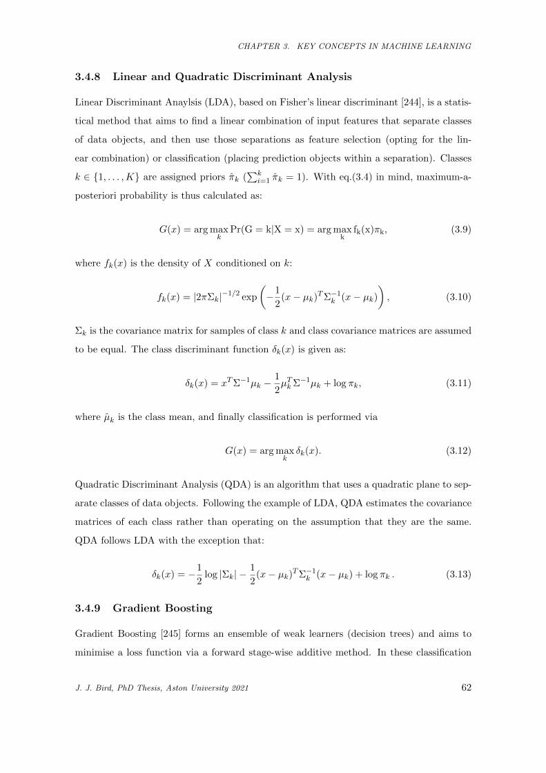
CHAPTER 3. KEY CONCEPTS IN MACHINE LEARNING
3.4.8 Linear and Quadratic Discriminant Analysis
Linear Discriminant Anaylsis (LDA), based on Fisher’s linear discriminant [244], is a statis-
tical method that aims to find a linear combination of input features that separate classes
of data objects, and then use those separations as feature selection (opting for the lin-
ear combination) or classification (placing prediction objects within a separation). Classes
k ∈ {1, . . . ,K} are assigned priors πk (∑k
i=1 πk = 1). With eq.(3.4) in mind, maximum-a-
posteriori probability is thus calculated as:
G(x) = argmaxk
Pr(G = k|X = x) = argmaxk
fk(x)πk, (3.9)
where fk(x) is the density of X conditioned on k:
fk(x) = |2πΣk|−1/2 exp
(−1
2(x− µk)
TΣ−1k (x− µk)
), (3.10)
Σk is the covariance matrix for samples of class k and class covariance matrices are assumed
to be equal. The class discriminant function δk(x) is given as:
δk(x) = xTΣ−1µk −1
2µTkΣ
−1µk + log πk, (3.11)
where µk is the class mean, and finally classification is performed via
G(x) = argmaxk
δk(x). (3.12)
Quadratic Discriminant Analysis (QDA) is an algorithm that uses a quadratic plane to sep-
arate classes of data objects. Following the example of LDA, QDA estimates the covariance
matrices of each class rather than operating on the assumption that they are the same.
QDA follows LDA with the exception that:
δk(x) = −1
2log |Σk| −
1
2(x− µk)
TΣ−1k (x− µk) + log πk . (3.13)
3.4.9 Gradient Boosting
Gradient Boosting [245] forms an ensemble of weak learners (decision trees) and aims to
minimise a loss function via a forward stage-wise additive method. In these classification
J. J. Bird, PhD Thesis, Aston University 2021 62
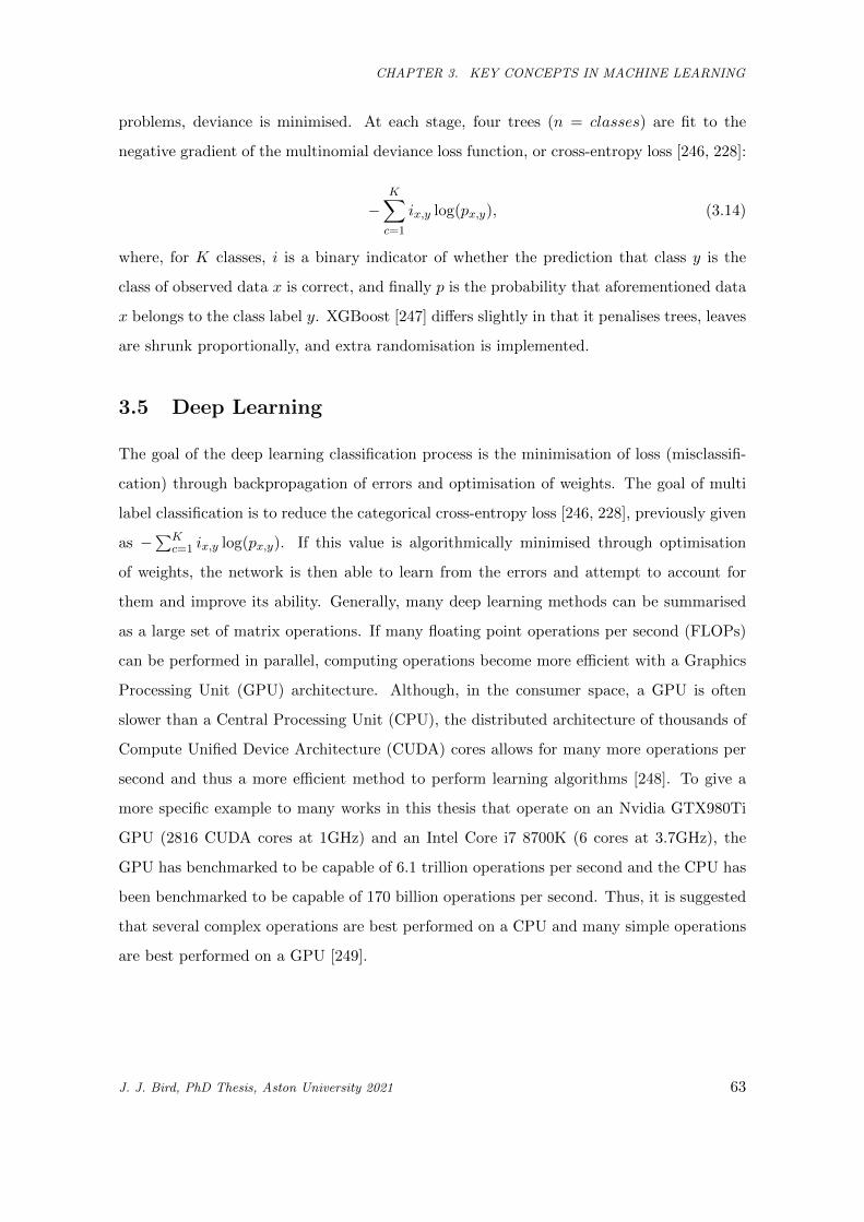
CHAPTER 3. KEY CONCEPTS IN MACHINE LEARNING
problems, deviance is minimised. At each stage, four trees (n = classes) are fit to the
negative gradient of the multinomial deviance loss function, or cross-entropy loss [246, 228]:
−K∑c=1
ix,y log(px,y), (3.14)
where, for K classes, i is a binary indicator of whether the prediction that class y is the
class of observed data x is correct, and finally p is the probability that aforementioned data
x belongs to the class label y. XGBoost [247] differs slightly in that it penalises trees, leaves
are shrunk proportionally, and extra randomisation is implemented.
3.5 Deep Learning
The goal of the deep learning classification process is the minimisation of loss (misclassifi-
cation) through backpropagation of errors and optimisation of weights. The goal of multi
label classification is to reduce the categorical cross-entropy loss [246, 228], previously given
as −∑K
c=1 ix,y log(px,y). If this value is algorithmically minimised through optimisation
of weights, the network is then able to learn from the errors and attempt to account for
them and improve its ability. Generally, many deep learning methods can be summarised
as a large set of matrix operations. If many floating point operations per second (FLOPs)
can be performed in parallel, computing operations become more efficient with a Graphics
Processing Unit (GPU) architecture. Although, in the consumer space, a GPU is often
slower than a Central Processing Unit (CPU), the distributed architecture of thousands of
Compute Unified Device Architecture (CUDA) cores allows for many more operations per
second and thus a more efficient method to perform learning algorithms [248]. To give a
more specific example to many works in this thesis that operate on an Nvidia GTX980Ti
GPU (2816 CUDA cores at 1GHz) and an Intel Core i7 8700K (6 cores at 3.7GHz), the
GPU has benchmarked to be capable of 6.1 trillion operations per second and the CPU has
been benchmarked to be capable of 170 billion operations per second. Thus, it is suggested
that several complex operations are best performed on a CPU and many simple operations
are best performed on a GPU [249].
J. J. Bird, PhD Thesis, Aston University 2021 63
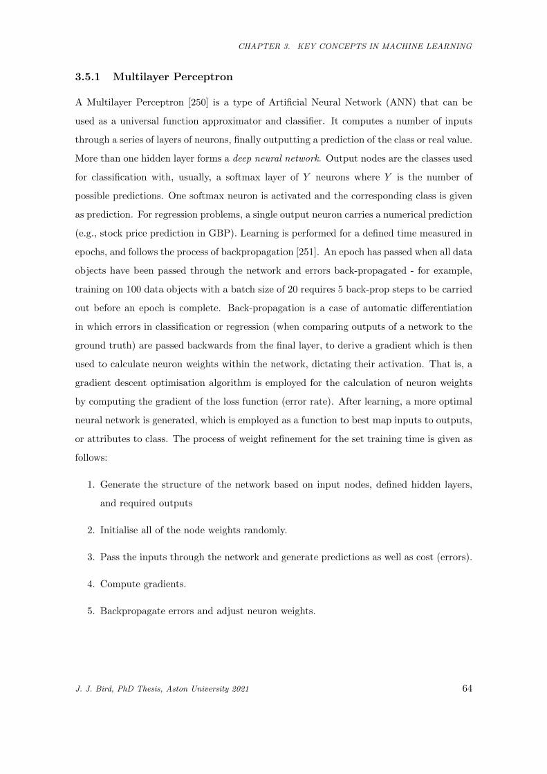
CHAPTER 3. KEY CONCEPTS IN MACHINE LEARNING
3.5.1 Multilayer Perceptron
A Multilayer Perceptron [250] is a type of Artificial Neural Network (ANN) that can be
used as a universal function approximator and classifier. It computes a number of inputs
through a series of layers of neurons, finally outputting a prediction of the class or real value.
More than one hidden layer forms a deep neural network. Output nodes are the classes used
for classification with, usually, a softmax layer of Y neurons where Y is the number of
possible predictions. One softmax neuron is activated and the corresponding class is given
as prediction. For regression problems, a single output neuron carries a numerical prediction
(e.g., stock price prediction in GBP). Learning is performed for a defined time measured in
epochs, and follows the process of backpropagation [251]. An epoch has passed when all data
objects have been passed through the network and errors back-propagated - for example,
training on 100 data objects with a batch size of 20 requires 5 back-prop steps to be carried
out before an epoch is complete. Back-propagation is a case of automatic differentiation
in which errors in classification or regression (when comparing outputs of a network to the
ground truth) are passed backwards from the final layer, to derive a gradient which is then
used to calculate neuron weights within the network, dictating their activation. That is, a
gradient descent optimisation algorithm is employed for the calculation of neuron weights
by computing the gradient of the loss function (error rate). After learning, a more optimal
neural network is generated, which is employed as a function to best map inputs to outputs,
or attributes to class. The process of weight refinement for the set training time is given as
follows:
1. Generate the structure of the network based on input nodes, defined hidden layers,
and required outputs
2. Initialise all of the node weights randomly.
3. Pass the inputs through the network and generate predictions as well as cost (errors).
4. Compute gradients.
5. Backpropagate errors and adjust neuron weights.
J. J. Bird, PhD Thesis, Aston University 2021 64
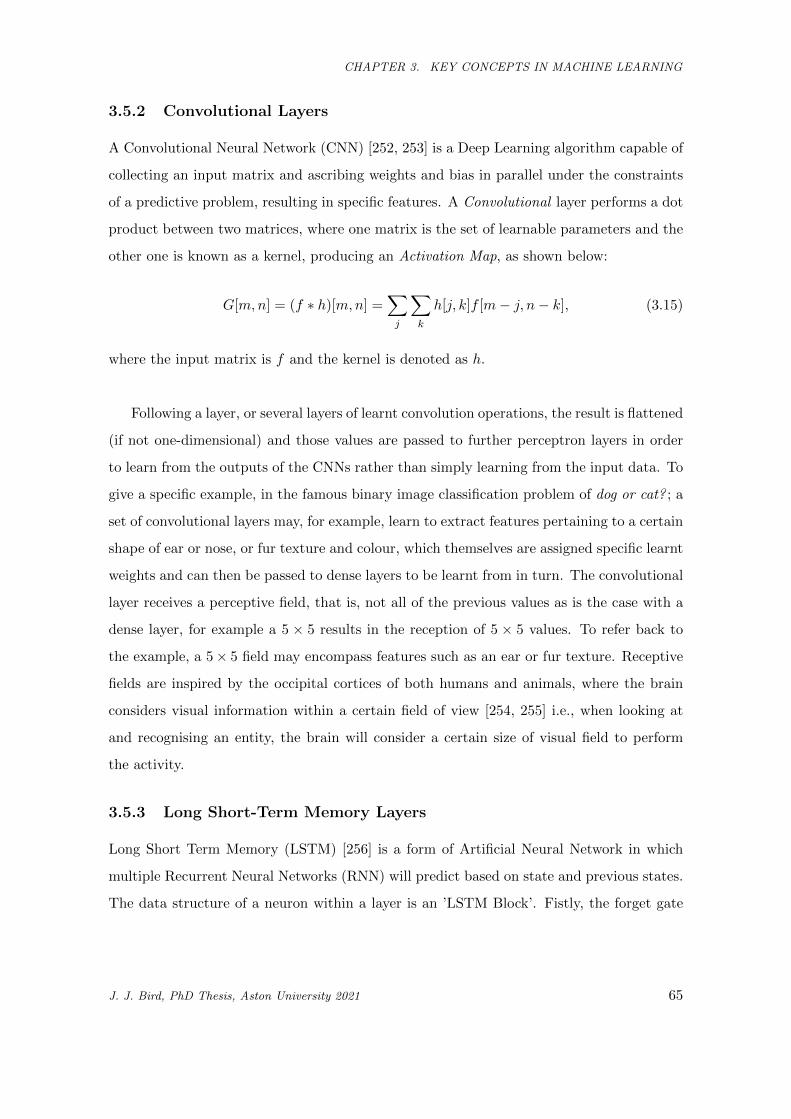
CHAPTER 3. KEY CONCEPTS IN MACHINE LEARNING
3.5.2 Convolutional Layers
A Convolutional Neural Network (CNN) [252, 253] is a Deep Learning algorithm capable of
collecting an input matrix and ascribing weights and bias in parallel under the constraints
of a predictive problem, resulting in specific features. A Convolutional layer performs a dot
product between two matrices, where one matrix is the set of learnable parameters and the
other one is known as a kernel, producing an Activation Map, as shown below:
G[m,n] = (f ∗ h)[m,n] =∑j
∑k
h[j, k]f [m− j, n− k], (3.15)
where the input matrix is f and the kernel is denoted as h.
Following a layer, or several layers of learnt convolution operations, the result is flattened
(if not one-dimensional) and those values are passed to further perceptron layers in order
to learn from the outputs of the CNNs rather than simply learning from the input data. To
give a specific example, in the famous binary image classification problem of dog or cat? ; a
set of convolutional layers may, for example, learn to extract features pertaining to a certain
shape of ear or nose, or fur texture and colour, which themselves are assigned specific learnt
weights and can then be passed to dense layers to be learnt from in turn. The convolutional
layer receives a perceptive field, that is, not all of the previous values as is the case with a
dense layer, for example a 5 × 5 results in the reception of 5 × 5 values. To refer back to
the example, a 5× 5 field may encompass features such as an ear or fur texture. Receptive
fields are inspired by the occipital cortices of both humans and animals, where the brain
considers visual information within a certain field of view [254, 255] i.e., when looking at
and recognising an entity, the brain will consider a certain size of visual field to perform
the activity.
3.5.3 Long Short-Term Memory Layers
Long Short Term Memory (LSTM) [256] is a form of Artificial Neural Network in which
multiple Recurrent Neural Networks (RNN) will predict based on state and previous states.
The data structure of a neuron within a layer is an ’LSTM Block’. Fistly, the forget gate
J. J. Bird, PhD Thesis, Aston University 2021 65
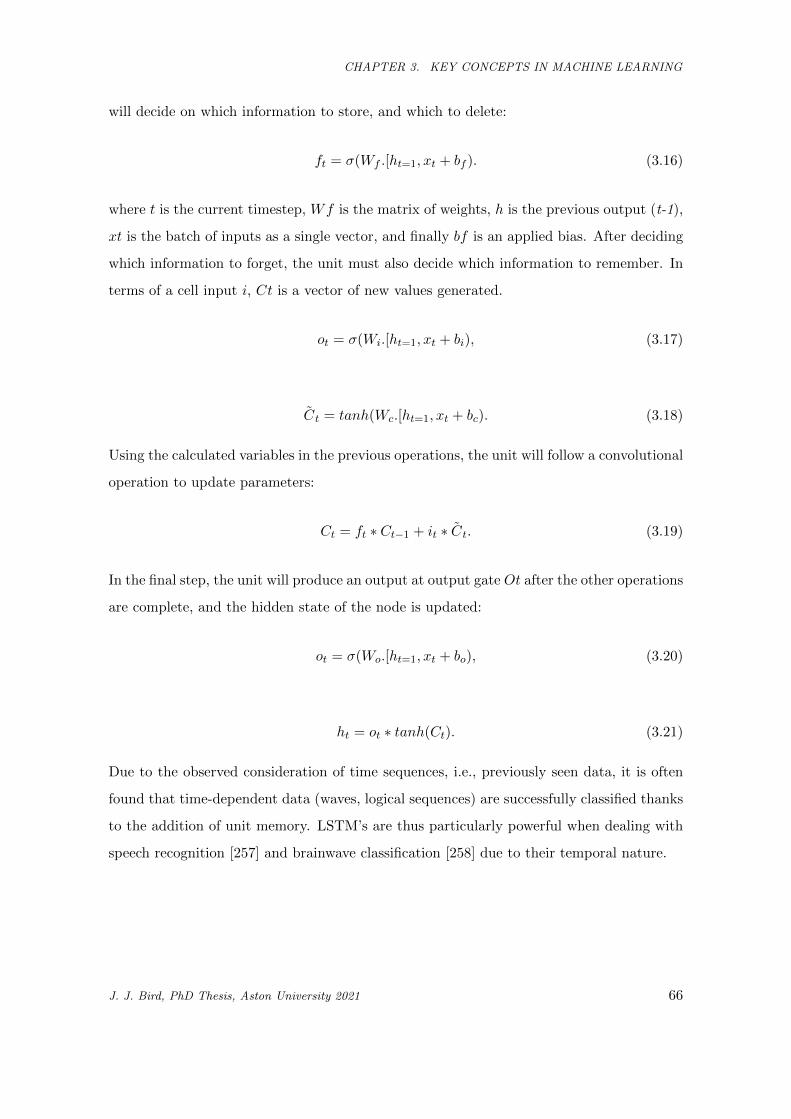
CHAPTER 3. KEY CONCEPTS IN MACHINE LEARNING
will decide on which information to store, and which to delete:
ft = σ(Wf .[ht=1, xt + bf ). (3.16)
where t is the current timestep, Wf is the matrix of weights, h is the previous output (t-1),
xt is the batch of inputs as a single vector, and finally bf is an applied bias. After deciding
which information to forget, the unit must also decide which information to remember. In
terms of a cell input i, Ct is a vector of new values generated.
ot = σ(Wi.[ht=1, xt + bi), (3.17)
Ct = tanh(Wc.[ht=1, xt + bc). (3.18)
Using the calculated variables in the previous operations, the unit will follow a convolutional
operation to update parameters:
Ct = ft ∗ Ct−1 + it ∗ Ct. (3.19)
In the final step, the unit will produce an output at output gate Ot after the other operations
are complete, and the hidden state of the node is updated:
ot = σ(Wo.[ht=1, xt + bo), (3.20)
ht = ot ∗ tanh(Ct). (3.21)
Due to the observed consideration of time sequences, i.e., previously seen data, it is often
found that time-dependent data (waves, logical sequences) are successfully classified thanks
to the addition of unit memory. LSTM’s are thus particularly powerful when dealing with
speech recognition [257] and brainwave classification [258] due to their temporal nature.
J. J. Bird, PhD Thesis, Aston University 2021 66
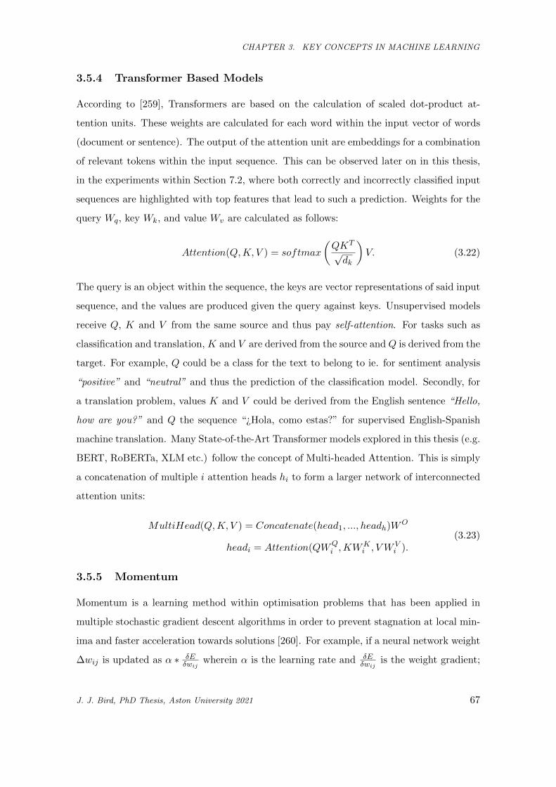
CHAPTER 3. KEY CONCEPTS IN MACHINE LEARNING
3.5.4 Transformer Based Models
According to [259], Transformers are based on the calculation of scaled dot-product at-
tention units. These weights are calculated for each word within the input vector of words
(document or sentence). The output of the attention unit are embeddings for a combination
of relevant tokens within the input sequence. This can be observed later on in this thesis,
in the experiments within Section 7.2, where both correctly and incorrectly classified input
sequences are highlighted with top features that lead to such a prediction. Weights for the
query Wq, key Wk, and value Wv are calculated as follows:
Attention(Q,K, V ) = softmax
(QKT
√dk
)V. (3.22)
The query is an object within the sequence, the keys are vector representations of said input
sequence, and the values are produced given the query against keys. Unsupervised models
receive Q, K and V from the same source and thus pay self-attention. For tasks such as
classification and translation, K and V are derived from the source andQ is derived from the
target. For example, Q could be a class for the text to belong to ie. for sentiment analysis
“positive” and “neutral” and thus the prediction of the classification model. Secondly, for
a translation problem, values K and V could be derived from the English sentence “Hello,
how are you?” and Q the sequence “¿Hola, como estas?” for supervised English-Spanish
machine translation. Many State-of-the-Art Transformer models explored in this thesis (e.g.
BERT, RoBERTa, XLM etc.) follow the concept of Multi-headed Attention. This is simply
a concatenation of multiple i attention heads hi to form a larger network of interconnected
attention units:
MultiHead(Q,K, V ) = Concatenate(head1, ..., headh)WO
headi = Attention(QWQi ,KWK
i , V W Vi ).
(3.23)
3.5.5 Momentum
Momentum is a learning method within optimisation problems that has been applied in
multiple stochastic gradient descent algorithms in order to prevent stagnation at local min-
ima and faster acceleration towards solutions [260]. For example, if a neural network weight
∆wij is updated as α ∗ δEδwij
wherein α is the learning rate and δEδwij
is the weight gradient;
J. J. Bird, PhD Thesis, Aston University 2021 67
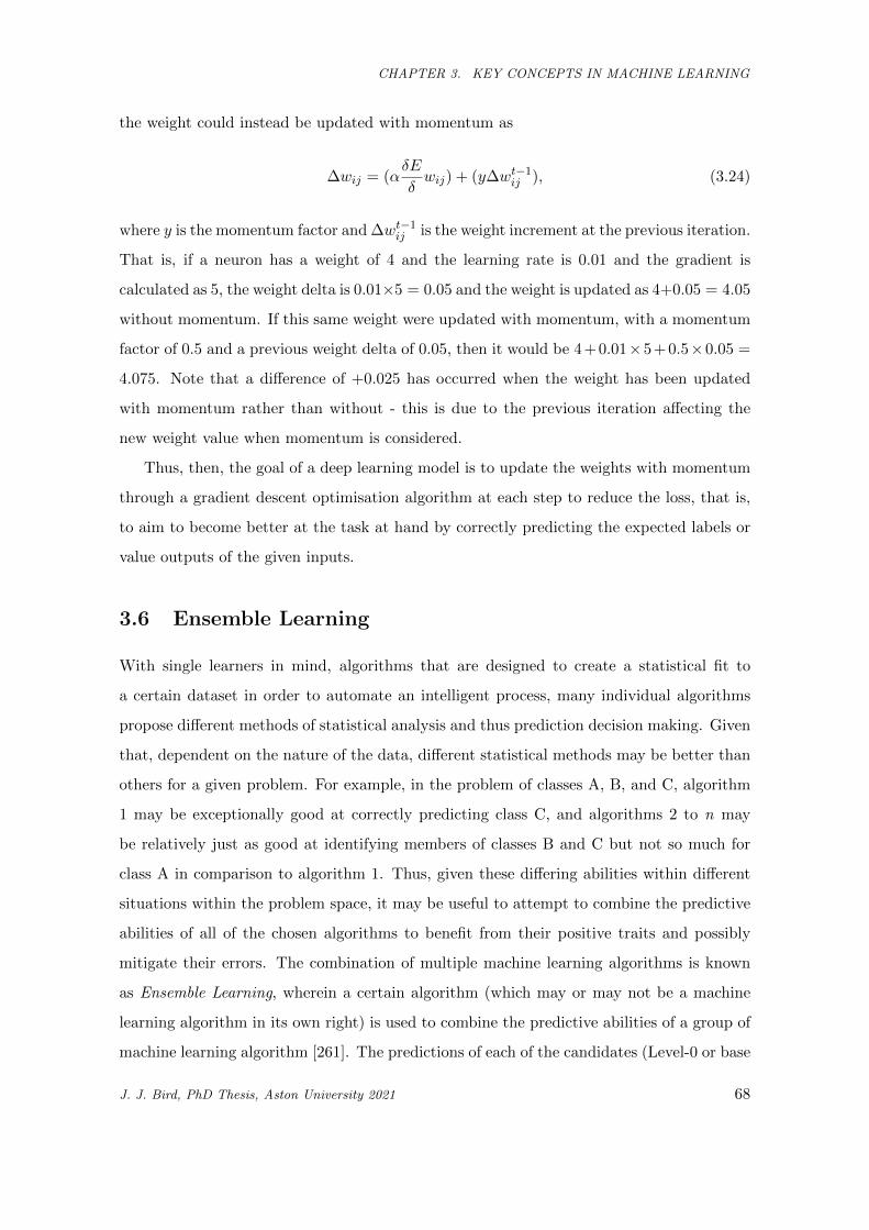
CHAPTER 3. KEY CONCEPTS IN MACHINE LEARNING
the weight could instead be updated with momentum as
∆wij = (αδE
δwij) + (y∆wt−1
ij ), (3.24)
where y is the momentum factor and ∆wt−1ij is the weight increment at the previous iteration.
That is, if a neuron has a weight of 4 and the learning rate is 0.01 and the gradient is
calculated as 5, the weight delta is 0.01×5 = 0.05 and the weight is updated as 4+0.05 = 4.05
without momentum. If this same weight were updated with momentum, with a momentum
factor of 0.5 and a previous weight delta of 0.05, then it would be 4+0.01×5+0.5×0.05 =
4.075. Note that a difference of +0.025 has occurred when the weight has been updated
with momentum rather than without - this is due to the previous iteration affecting the
new weight value when momentum is considered.
Thus, then, the goal of a deep learning model is to update the weights with momentum
through a gradient descent optimisation algorithm at each step to reduce the loss, that is,
to aim to become better at the task at hand by correctly predicting the expected labels or
value outputs of the given inputs.
3.6 Ensemble Learning
With single learners in mind, algorithms that are designed to create a statistical fit to
a certain dataset in order to automate an intelligent process, many individual algorithms
propose different methods of statistical analysis and thus prediction decision making. Given
that, dependent on the nature of the data, different statistical methods may be better than
others for a given problem. For example, in the problem of classes A, B, and C, algorithm
1 may be exceptionally good at correctly predicting class C, and algorithms 2 to n may
be relatively just as good at identifying members of classes B and C but not so much for
class A in comparison to algorithm 1. Thus, given these differing abilities within different
situations within the problem space, it may be useful to attempt to combine the predictive
abilities of all of the chosen algorithms to benefit from their positive traits and possibly
mitigate their errors. The combination of multiple machine learning algorithms is known
as Ensemble Learning, wherein a certain algorithm (which may or may not be a machine
learning algorithm in its own right) is used to combine the predictive abilities of a group of
machine learning algorithm [261]. The predictions of each of the candidates (Level-0 or base
J. J. Bird, PhD Thesis, Aston University 2021 68
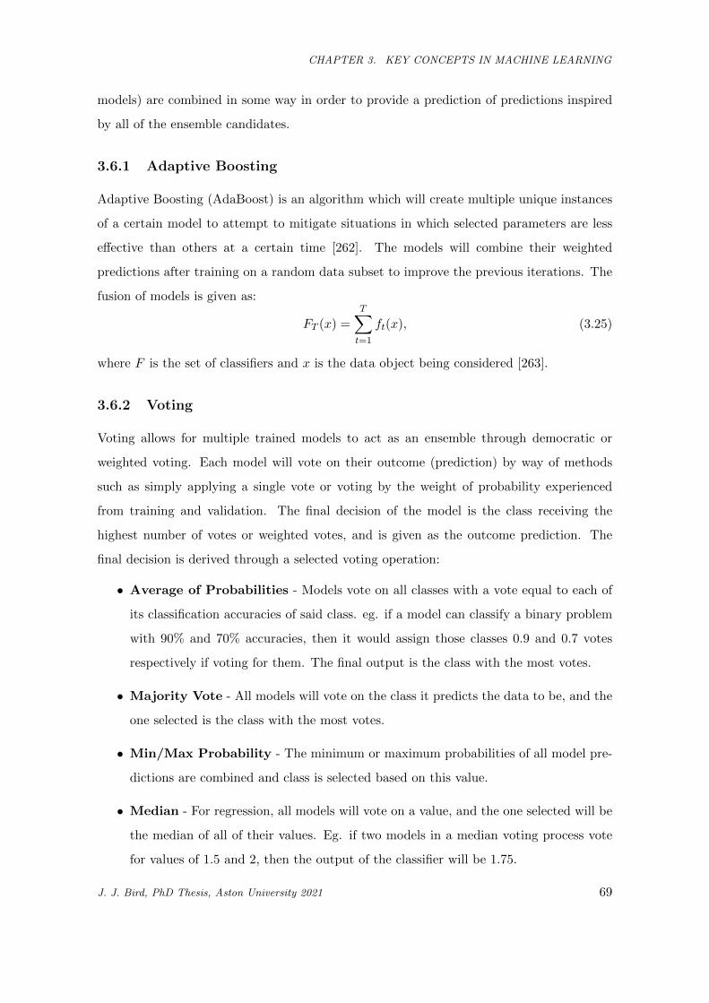
CHAPTER 3. KEY CONCEPTS IN MACHINE LEARNING
models) are combined in some way in order to provide a prediction of predictions inspired
by all of the ensemble candidates.
3.6.1 Adaptive Boosting
Adaptive Boosting (AdaBoost) is an algorithm which will create multiple unique instances
of a certain model to attempt to mitigate situations in which selected parameters are less
effective than others at a certain time [262]. The models will combine their weighted
predictions after training on a random data subset to improve the previous iterations. The
fusion of models is given as:
FT (x) =T∑t=1
ft(x), (3.25)
where F is the set of classifiers and x is the data object being considered [263].
3.6.2 Voting
Voting allows for multiple trained models to act as an ensemble through democratic or
weighted voting. Each model will vote on their outcome (prediction) by way of methods
such as simply applying a single vote or voting by the weight of probability experienced
from training and validation. The final decision of the model is the class receiving the
highest number of votes or weighted votes, and is given as the outcome prediction. The
final decision is derived through a selected voting operation:
• Average of Probabilities - Models vote on all classes with a vote equal to each of
its classification accuracies of said class. eg. if a model can classify a binary problem
with 90% and 70% accuracies, then it would assign those classes 0.9 and 0.7 votes
respectively if voting for them. The final output is the class with the most votes.
• Majority Vote - All models will vote on the class it predicts the data to be, and the
one selected is the class with the most votes.
• Min/Max Probability - The minimum or maximum probabilities of all model pre-
dictions are combined and class is selected based on this value.
• Median - For regression, all models will vote on a value, and the one selected will be
the median of all of their values. Eg. if two models in a median voting process vote
for values of 1.5 and 2, then the output of the classifier will be 1.75.
J. J. Bird, PhD Thesis, Aston University 2021 69
CHAPTER 3. KEY CONCEPTS IN MACHINE LEARNING
3.6.3 Random Forests
A Random Forest [264] is an ensemble of Random Trees through Bootstrap Aggregating
(bagging) and Voting. Training is performed through a bagging process where multiple
random decision trees are generated, a random selection of data is gathered, and trees are
grown to fit the set. Once the training is completed, the generated trees will all vote, and
the majority vote is selected as the predicted class. Random Forests tend to outperform
Random Trees due to their decreasing of variance without increasing of the model bias.
3.6.4 Stacking
Stacking, or Stacked Generalisation, is a method of ensembling models and having their
predictive outputs form a meta dataset for interpretation [265]. The models to be ensembled
are known as either base models or Level-0 Models, which are trained on the training data
and then output their predictions for the testing data through the selected validation method
(i.e. operating as normal). Following this, the meta model, or Level-1 Model interprets
these predictions and produces a final prediction based on them. For example, if three
selected machine learning models (Level-0 models) were to output ’Dog’, ’Dog’, and ’Cat’
respectively; a selected Level-1 Model then receives not the data but these predictions as
input and learns patterns within them. The model could simply learn that a standard
majority vote is apt for the models and as such would predict the label ’Dog’, but, if the
meta-model had learnt that the third base model was specifically very good at recognising
the ’Cat’ label (especially if the first two do not) then it could predict the ’Cat’ label. The
latter may not be a democratic process as was described in the voting section, but may
statistically lead to a better overall score when considering the testing dataset predictions.
To give a simplified description, stacking is the process of learning from an ensemble’s
predictions by the interpretation of these predictions by a decision-making machine learning
algorithm.
3.7 Errors
Errors in regression can be calculated in numerous ways, for example, the value difference
or Root Mean Squared Error (RMSE), i.e. a prediction of 100,000 for a real value 90,000
would result in a RMSE of 10,000. In classification, a measure of entropy is often used, i.e.,
J. J. Bird, PhD Thesis, Aston University 2021 70
CHAPTER 3. KEY CONCEPTS IN MACHINE LEARNING
the level of randomness or predictability for the classification of a set (see Equation 3.14).
Comparing the difference of model entropies gives the Information Gain (relative entropy)
or Kullback-Leibler Divergence (KLD). This is when a univariate probability distribution of
a given attribute is compared to another [228]. The calculation with the entropy algorithm
in mind is thus simply given as:
InfoGain(T, a) = E(T )− E(T |a), (3.26)
that is, with E of Equation 3.14 in mind, the observed change in entropy. For instances of
original ruleset H(T ) and comparative ruleset H(T |a). A positive Information Gain denotes
a lower error rate and thus arguably a better model2.
3.8 Evolutionary Topology Search
The optimal number of hidden layers and neurons (topology structure) for a given network
is largely data dependent. A combinatorial optimisation problem thus occurs, and there is
no simple linear algorithm to derive the optimal solution - there is no free lunch [266]. Since
fully connected neural networks produce a relatively small search space as the connections
themselves are assumed, an optimisation approach for the network topology is a realistic
search problem.
Denser is an alternative novel method of evolutionary optimisation of an MLP [267].
In addition to the number of hidden layers and neurons within fully connected neural
networks, Denser also considers the type of layer itself. This increase of parameters results
in a very complex search space and is subsequently a computationally intensive algorithm.
However, it achieves very high accuracy results, for example, 93.29% on the CIFAR-10
image recognition dataset.
Evolution of Neural Networks through Augmenting Topologies (NEAT) is an algorithm
for the genetic improvement of neural networks which are not necessarily fully connected
between layers [268]. The algorithm has been observed to be effective in learning from user
input problems, such as playing games, for example an evolving ANN that learns to play
Super Mario in real time [269].
In EvoDeep [270], an evolutionary algorithm used to derive a deep neural network for
2When a balanced dataset is considered.
J. J. Bird, PhD Thesis, Aston University 2021 71
CHAPTER 3. KEY CONCEPTS IN MACHINE LEARNING
deep learning (eg. LSTM), researchers found Roulette Selection (random) for each popula-
tion member to be best in the solution breeding process, therefore this method was chosen
for the hyperheuristic evolutionary searches in multiple experiments within this thesis. That
is, each solution is in turn treated as px and a random second solution from solutions− 1
is chosen as py and an offspring solution F (px, py) = oxy is produced by breeding algorithm
F .
Deep Evolutionary Multilayer Perceptron, or DEvo, is an approach to optimising a Neu-
ral Network topology through evolutionary computation. Networks are treated as individual
organisms in the process where their classification ability dictates their fitness metric, thus
it is a single-objective algorithm. The pseudocode for the algorithm is given in Algorithm
1. The process to combine two networks follows the aforementioned work, where the depth
of the hidden layers is decided by selecting one of the two parents at random or mutation
at a defined random chance. Then, for each layer, the number of neurons is decided by
selecting the nth layer of either parent at random (provided both parent networks have
an nth layer), again the mutation chance then dictates a random mutation resulting in the
number of neurons being a random number between 1 and maxNeurons. Once the network
structure is generated, a pre-selected gradient descent problem is initiated and the network
learns through backpropagation. The solution’s performance, i.e., increases of accuracy,
minimisation of loss, etc., is considered as fitness, and the weaker solutions are culled. This
process is repeated with the goal of tuning the improved topologies for the problem at hand,
and results in a final generation containing the strongest solutions found throughout the
simulation.
Thus, after simulation, the goal of the algorithm is to derive a more effective neural
network topology for the given dataset. The algorithm is implemented due to neural net-
work hyper-parameter tuning being a non-polynomial problem [271]. The algorithm can be
computationally expensive; a ten population roulette breeding simulation executed for ten
generations would produce 120 neural networks to be trained, since eleven are produced
every generation. Resource usage is thus high for the simulation, but the final result gives a
network topology apt for the given data, and this finding can be used in further experiments.
The process followed can also be observed in the Flowchart (Figure 3.1). Therefore, it can
be considered that an evolutionary topology search engineers a problem space for a gradient
descent optimiser, since the network structure itself is optimised by the evolutionary search
J. J. Bird, PhD Thesis, Aston University 2021 72
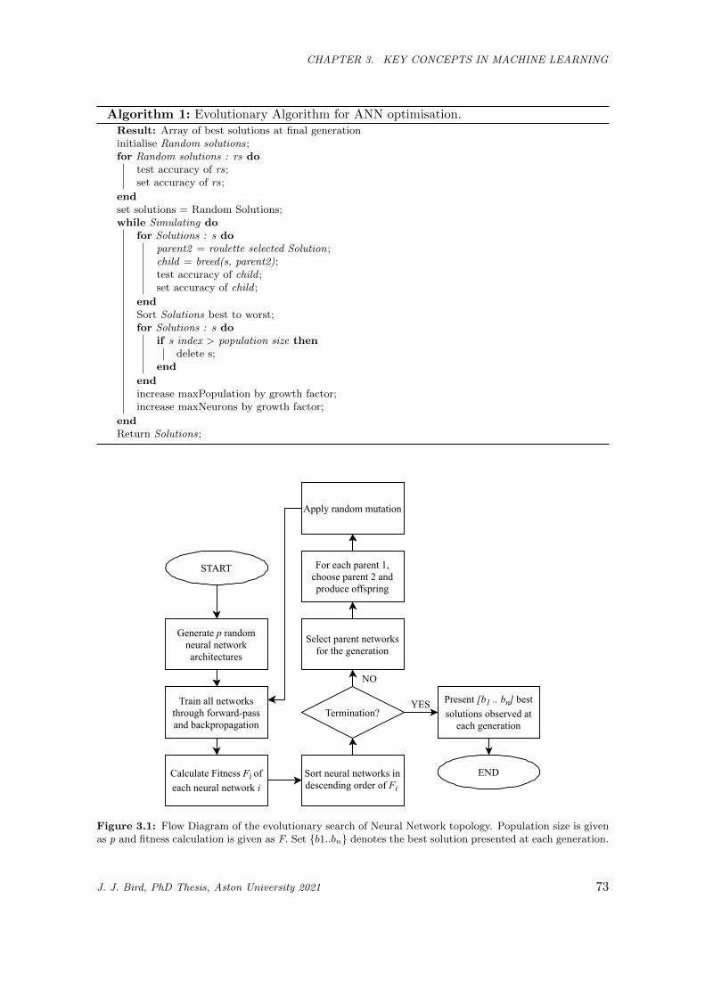
CHAPTER 3. KEY CONCEPTS IN MACHINE LEARNING
Algorithm 1: Evolutionary Algorithm for ANN optimisation.Result: Array of best solutions at final generationinitialise Random solutions;for Random solutions : rs do
test accuracy of rs;set accuracy of rs;
endset solutions = Random Solutions;while Simulating do
for Solutions : s doparent2 = roulette selected Solution;child = breed(s, parent2);test accuracy of child ;set accuracy of child ;
endSort Solutions best to worst;for Solutions : s do
if s index > population size thendelete s;
end
endincrease maxPopulation by growth factor;increase maxNeurons by growth factor;
endReturn Solutions;
START
Generateprandomneuralnetworkarchitectures
Trainallnetworksthroughforward-passandbackpropagation
CalculateFitnessFiofeachneuralnetworki
SortneuralnetworksindescendingorderofFi
Selectparentnetworksforthegeneration
Termination?
Foreachparent1,chooseparent2andproduceoffspring
Applyrandommutation
Present[b1..bn]bestsolutionsobservedateachgeneration
END
NO
YES
Figure 3.1: Flow Diagram of the evolutionary search of Neural Network topology. Population size is givenas p and fitness calculation is given as F. Set {b1..bn} denotes the best solution presented at each generation.
J. J. Bird, PhD Thesis, Aston University 2021 73
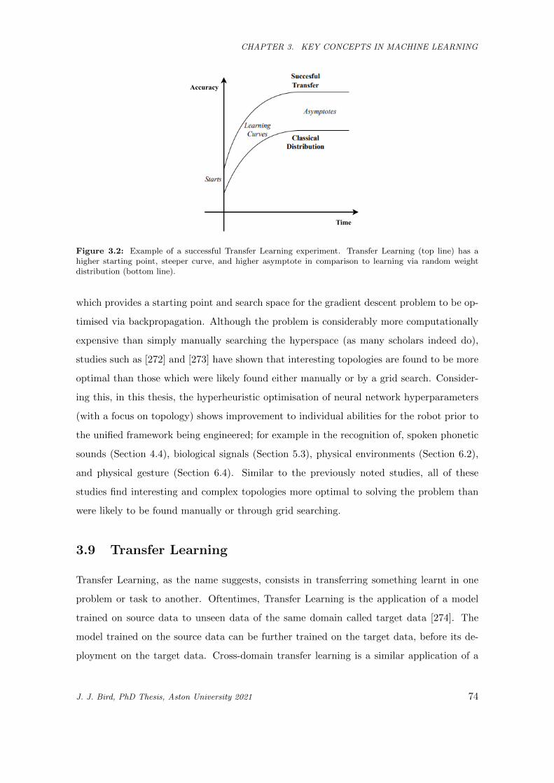
CHAPTER 3. KEY CONCEPTS IN MACHINE LEARNING
Accuracy
Time
Figure 3.2: Example of a successful Transfer Learning experiment. Transfer Learning (top line) has ahigher starting point, steeper curve, and higher asymptote in comparison to learning via random weightdistribution (bottom line).
which provides a starting point and search space for the gradient descent problem to be op-
timised via backpropagation. Although the problem is considerably more computationally
expensive than simply manually searching the hyperspace (as many scholars indeed do),
studies such as [272] and [273] have shown that interesting topologies are found to be more
optimal than those which were likely found either manually or by a grid search. Consider-
ing this, in this thesis, the hyperheuristic optimisation of neural network hyperparameters
(with a focus on topology) shows improvement to individual abilities for the robot prior to
the unified framework being engineered; for example in the recognition of, spoken phonetic
sounds (Section 4.4), biological signals (Section 5.3), physical environments (Section 6.2),
and physical gesture (Section 6.4). Similar to the previously noted studies, all of these
studies find interesting and complex topologies more optimal to solving the problem than
were likely to be found manually or through grid searching.
3.9 Transfer Learning
Transfer Learning, as the name suggests, consists in transferring something learnt in one
problem or task to another. Oftentimes, Transfer Learning is the application of a model
trained on source data to unseen data of the same domain called target data [274]. The
model trained on the source data can be further trained on the target data, before its de-
ployment on the target data. Cross-domain transfer learning is a similar application of a
J. J. Bird, PhD Thesis, Aston University 2021 74
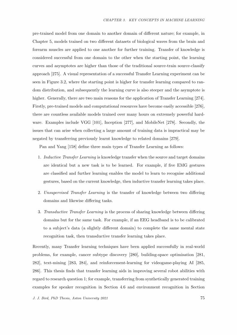
CHAPTER 3. KEY CONCEPTS IN MACHINE LEARNING
pre-trained model from one domain to another domain of different nature; for example, in
Chapter 5, models trained on two different datasets of biological waves from the brain and
forearm muscles are applied to one another for further training. Transfer of knowledge is
considered successful from one domain to the other when the starting point, the learning
curves and asymptotes are higher than those of the traditional source-train source-classify
approach [275]. A visual representation of a successful Transfer Learning experiment can be
seen in Figure 3.2, where the starting point is higher for transfer learning compared to ran-
dom distribution, and subsequently the learning curve is also steeper and the asymptote is
higher. Generally, there are two main reasons for the application of Transfer Learning [274].
Firstly, pre-trained models and computational resources have become easily accessible [276],
there are countless available models trained over many hours on extremely powerful hard-
ware. Examples include VGG [101], Inception [277], and MobileNet [278]. Secondly, the
issues that can arise when collecting a large amount of training data is impractical may be
negated by transferring previously learnt knowledge to related domains [279].
Pan and Yang [158] define three main types of Transfer Learning as follows:
1. Inductive Transfer Learning is knowledge transfer when the source and target domains
are identical but a new task is to be learned. For example, if five EMG gestures
are classified and further learning enables the model to learn to recognise additional
gestures, based on the current knowledge, then inductive transfer learning takes place.
2. Unsupervised Transfer Learning is the transfer of knowledge between two differing
domains and likewise differing tasks.
3. Transductive Transfer Learning is the process of sharing knowledge between differing
domains but for the same task. For example, if an EEG headband is to be calibrated
to a subject’s data (a slightly different domain) to complete the same mental state
recognition task, then transductive transfer learning takes place.
Recently, many Transfer learning techniques have been applied successfully in real-world
problems, for example, cancer subtype discovery [280], building-space optimisation [281,
282], text-mining [283, 284], and reinforcement-learning for videogame-playing AI [285,
286]. This thesis finds that transfer learning aids in improving several robot abilities with
regard to research question 1; for example, transferring from synthetically generated training
examples for speaker recognition in Section 4.6 and environment recognition in Section
J. J. Bird, PhD Thesis, Aston University 2021 75
CHAPTER 3. KEY CONCEPTS IN MACHINE LEARNING
Real Augmented 1 Augmented 2 Augmented 3 Augmented 4
Figure 3.3: A real image of the Pepper Robot (left) followed by four examples of augmented images.Augmentation techniques involve offsets, scaling, rotation and mirroring.
6.3, gesture recognition by electromyographical calibration in Section 5.5 and between sign
languages in Section 6.4, and signal classification between the domains of electromyography
and electroencephalography in Section 5.7.
3.10 Data Augmentation
Data augmentation is the process of artificially expanding a training dataset via generating
new data samples through modification of the available data [287]. Augmentation can
be performed by simple approaches, such as injection of Gaussian noise into a numerical
dataset [288], or by more complex algorithms such as repurposing models described in this
chapter to perform a generative approach. That is, rather than training to recognise data, a
model can be trained to generate similar data that, if given as an input, would be classified as
belonging to the real data. For example, work has found that using a Deep Convolutional
Generative Adversarial Network (DCGAN) can augment a dataset for improved image
classification [289], which is especially important when training examples may be scarce.
The goal of the GAN is to train two concatenated neural networks, the first learns to
generate a data object while the second learns to discriminate between what is real and
what is not. Thus, the two networks train adversarially by competing against one another.
This training process leads to the generator being able to create higher quality outputs that
contain useful knowledge to improve an algorithm through training data augmentation3.
Data augmentation is best visualised, as can be seen in Figure 3.3. In these examples,
offset, scale, rotation, and mirroring techniques are used to create new data objects from the
first. Although from a human perspective all of the images are obviously of the same robot, if
the matrix operations of a CNN are considered, varying outputs would be generated. Thus,
3Further detail on GANs can be found in [290].
J. J. Bird, PhD Thesis, Aston University 2021 76
CHAPTER 3. KEY CONCEPTS IN MACHINE LEARNING
to the network, these provide more knowledge such as how an entity would be seen at an
angle, and therefore provide training examples that increase the training and classification
ability of the model.
It is due to this nature of CNNs that many examples of augmented training in literature
within the domain of image recognition. Although this is the case, the growing improved
generative ability of models such as new types of GAN and Transformer architectures have
enabled augmented improvement to gesture recognition [174], biological signal classifica-
tion [175], speech recognition [291], and human activity recognition [292] among many
others. In this thesis, it is explored how data augmentation can improve the Human-Robot
Interaction experience through improved autonomous abilities; for example the improve-
ment of, speaker recognition models in Section 4.3 where LSTMs and transformers are
used to generate new speech data, biological signal classification in Section 5.6 where a
transformer architecture learns to generate useful new signals, environment recognition in
Section 6.3 through training augmentation by simulated environments applied to the real
world, and finally the improvement of a transformer-based chatbot to provide natural input
to the framework by synthetically generating more human examples of written phrases via
parpahrasing in Section 7.2.
3.11 Summary
To summarise, this chapter has presented the methods by which modern machines learn.
In a classical learning sense, algorithms are run to increase a metric from validation data,
such as classification accuracy. Given a balanced dataset, if an algorithm can classify more
data objects correctly, therein lies an argument that the algorithm could be used for fur-
ther unknown data points (i.e., in production). Following on from this, this chapter also
described deep learning, the process of engineering weights within a network via backpropa-
gation and gradient descent. Although more complex and requiring far more computational
resources than their classical counterparts, the notion of deep learning has overtaken them
to become the current state-of-the-art in machine intelligence due to both current findings
and potential future capabilities.
Following the basis of machine learning, further techniques were also explored. This
included the idea of fusing the differing capabilities of individual models for a unified pre-
J. J. Bird, PhD Thesis, Aston University 2021 77

CHAPTER 3. KEY CONCEPTS IN MACHINE LEARNING
diction, and the methods used that can create such an ensemble. Furthermore important
to this thesis were the concepts of transferring weights from one deep learning domain to
another, as well as augmenting datasets with synthetic data objects to improve learning
ability. The techniques and algorithms described in this chapter are to be encountered
throughout this thesis, both as tools to achieve certain robotic abilities, and in the bench-
marking of improving both model and ability such as through transfer learning and data
augmentation. These methods have thus been presented in this unified chapter given that
they feature prominently throughout the remainder of this thesis.
J. J. Bird, PhD Thesis, Aston University 2021 78
CHAPTER 4. VERBAL HUMAN-ROBOT INTERACTION
Chapter 4
Verbal Human-Robot Interaction
4.1 Introduction
It is no surprise that human speech and writing do not convey the same amount of informa-
tion as one another. When conversing, the act of speech contains more useful information
than just words. Verbal introduction in Human-Robot Interaction is an interaction where
input is given as the operator’s voice. This chapter explores voice-based interaction mod-
ules for the final framework in the form of Speaker Recognition, phoneme recognition in
audio for both phoneme and accent classification, synthesis of speech (based on learning
from a real voice), and finally sentiment analysis for classification of five levels of sentiment.
Along with the classification ability of speech, a multi-objective approach is also explored
given that efficiency of tasks is also important in HRI[293]. Given that there is a common
theme underlying these technologies, namely feature extraction of audio, this is explored
initially prior to the aforementioned experiments being presented in their own sections. As
was discussed in the introduction, the scientific contributions of individual experiments are
presented where appropriate within the section introductions.
4.2 Feature Extraction from Audio
The audio feature extraction that takes place within this chapter for speech, and in Chap-
ter 6 scene sounds follows the process of extracting Mel Frequency Cepstral Coefficients
(MFCCs) in order to provide a numerical vector representative of the behaviour of sound
over time. Here, the process is explained. The specific hyperparameters such as window
J. J. Bird, PhD Thesis, Aston University 2021 79
CHAPTER 4. VERBAL HUMAN-ROBOT INTERACTION
length and overlap differ between experiments, and thus are given in the appropriate section.
Since audio waves are complex and non-stationary, classification of the raw data poses
a difficult problem [294]. Due to this, numerical statistical features must be extracted from
the data in order to provide useful input to a model. This thesis focuses mainly on the
the Mel-Frequency Cepstral Coefficients (MFCC) [35] of the audio clips through a set of
sliding windows 0.25s in length (ie frame size of 4K sampling points) and an additional
set of overlapping windows, thus producing 8 sliding windows, i.e., 8 frames/sec. MFCC
extraction is described as follows:
1. The Fourier Transform (FT) of the time window data ω is derived via:
X(jω) =
∫ ∞
−∞x(t)e−jωtdt. (4.1)
2. The powers from the FT are mapped to the Mel scale, the psychological scale of
audible pitch [295]. This occurs through the use of a triangular temporal window.
3. The Mel-Frequency Cepstrum (MFC), or power spectrum of sound, is considered and
logs of each of their powers are taken.
4. The derived Mel-log powers are treated as a signal, and a Discrete Cosine Transform
(DCT) is measured. This is given as:
Xk =N−1∑n=0
xncos[πN (n+ 1
2)k]k = 0, ..., N − 1, (4.2)
where x is the array of length N , k is the index of the output coefficient being cal-
culated, where N real numbers x0...xn−1 are transformed into the N real numbers
X0...Xn−1 by the formula.
The amplitudes of the spectrum are known as the MFCCs. The resultant data then provides
a mathematical description of audio behaviour and are useful for classification of sound.
4.3 Synthetic Data Augmentation for Speaker Recognition
Data scarcity is an issue that arises often outside of the lab, due to the large amount of data
required for classification activities. This includes speaker classification in order to enable
J. J. Bird, PhD Thesis, Aston University 2021 80
CHAPTER 4. VERBAL HUMAN-ROBOT INTERACTION
personalised Human-Machine (HMI) and Human-Robot Interaction (HRI), a technology
growing in consumer usefulness within smart device biometric security on devices such as
smartphones and tablets, as well as for multiple-user smarthome assistants (operating on
a per-person basis) which are not yet available. Speaker recognition, i.e., autonomously
recognising a person from their voice, is a well-explored topic in the state-of-the-art within
the bounds of data availability, which causes difficulty in real-world use. It is unrealistic to
expect a user to willingly provide many minutes or hours of speech data to a device unless
the device is allowed to constantly record daily life, which is a cause for concern with the
virtual home assistant. This study has shown that data scarcity in speaker recognition can
be overcome by collecting only several short spoken sentences of audio from a user and
then using extracted Mel-Frequency Cepstral Coefficients (MFCC) data in both supervised
and unsupervised learning paradigms to generate synthetic speech, which is then used in a
process of transfer learning to better recognise the speaker in question.
Autonomous speaker classification can suffer issues of data scarcity since the user is
compared to a large database of many speakers. The most obvious solution to this is to
collect more data from the speaker, but with the existence of Smart Home Assistants within
private environments, potentially listening to private data, this produces an obvious problem
of privacy and security [296, 297]. Not collecting more data on the other hand, presents
an issue of a large class imbalance between the speaker to classify against the examples of
other speakers, leading to lower accuracy and less trustworthy results [298], which must be
overcome for purposes such as biometrics, since the results must be trusted when used for
security. In this study, weighting of errors is performed to introduce balance, but it is noted
that the results still have room for improvement regardless.
Through data augmentation, useful new data can be generated by algorithms or models
that would improve the classification of the original, scarce dataset. A simple but prominent
example of this is the warping, flipping, mirroring, and noising of images to better prepare
image classification algorithms [299]. A more complex example through generative models
can be seen in recent works that utilise methods such as the Generative Adversarial Network
(GAN) to create synthetic data, which itself also holds useful information for learning from
and classification of data [300, 301]. Although image classification is the most common
and most obvious application of generative models for data augmentation, recent works
have also enjoyed success in augmenting audio data for sound classification [302, 303]. The
J. J. Bird, PhD Thesis, Aston University 2021 81
CHAPTER 4. VERBAL HUMAN-ROBOT INTERACTION
contributions of this section are three-fold:
1. The dataset is extended to more subjects from multiple international backgrounds and
the extraction of the Mel-Frequency Cepstral Coefficients (MFCCs) of each subject.
2. Speakers are recognised against the Flickr8k and Fluent Speech Commands datasets.
3. Benchmarking of a Long Short Term Memory (LSTM) architecture for 64, 128, 256
and 512 LSTM units in one to three hidden layers towards reduction of loss in gen-
erating synthetic data is performed. The best model is selected as the candidate for
the LSTM data generator.
4. OpenAI’s GPT-2 model is included as a data generator in order to compare the
approaches of supervised (LSTM) and attention-based (GPT-2) methods for synthetic
data augmentation for speaker classification.
The scientific contributions of this work, thus, are related to the application of synthetic
MFCCs for the improvement of speaker recognition. The best LSTM and the GPT-2 model
are tasked with generating 2,500, 5,000, 7,500, and 10,000 synthetic data objects for each
subject after learning from the scarce datasets extracted from their speech. A network then
learns from these data and transfers their weights to another network aiming to learn and
classify the real data. In many cases there is an improvement. For all subjects, several of
the networks perform best after experiencing exposure to synthetic data.
4.3.1 Method
In this section the development of the proposed approach is described, as illustrated overall
in Figure 4.1. For each test, five networks are trained. Firstly, a network is trained simply
to perform the speaker classification experiment without transfer learning (from a standard
random weight distribution). Produced by LSTM and GPT-2, synthetic data are used to
train another network, of which the weights are used to train the final network as an initial
distribution to perform the same experiment as described in the first network (classifying
the speaker’s real data from Flickr8k/Fluent Speech Commands speakers). Thus, the two
networks leading to the final classification score in the diagram are directly comparable
since they are learning from the same data, and they differ only in initial weight distribution
(where the latter network has weights learnt from synthetic data).
J. J. Bird, PhD Thesis, Aston University 2021 82
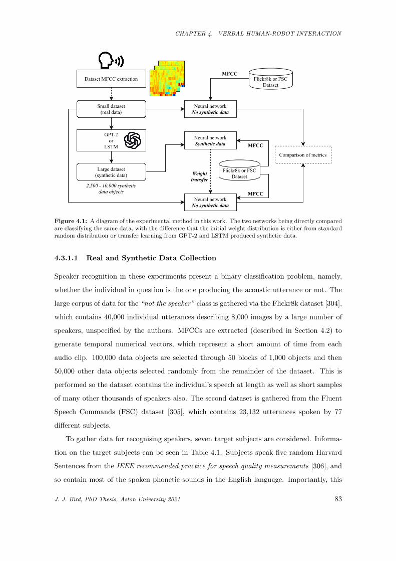
CHAPTER 4. VERBAL HUMAN-ROBOT INTERACTION
Smalldataset(realdata)
GPT-2or
LSTM
Largedataset(syntheticdata)
Comparisonofmetrics
NeuralnetworkNosyntheticdata
2,500-10,000syntheticdataobjects
NeuralnetworkSyntheticdata
NeuralnetworkNosyntheticdata
Weighttransfer
Flickr8korFSCDataset
DatasetMFCCextraction Flickr8korFSCDataset
MFCC
MFCC
MFCC
Figure 4.1: A diagram of the experimental method in this work. The two networks being directly comparedare classifying the same data, with the difference that the initial weight distribution is either from standardrandom distribution or transfer learning from GPT-2 and LSTM produced synthetic data.
4.3.1.1 Real and Synthetic Data Collection
Speaker recognition in these experiments present a binary classification problem, namely,
whether the individual in question is the one producing the acoustic utterance or not. The
large corpus of data for the “not the speaker” class is gathered via the Flickr8k dataset [304],
which contains 40,000 individual utterances describing 8,000 images by a large number of
speakers, unspecified by the authors. MFCCs are extracted (described in Section 4.2) to
generate temporal numerical vectors, which represent a short amount of time from each
audio clip. 100,000 data objects are selected through 50 blocks of 1,000 objects and then
50,000 other data objects selected randomly from the remainder of the dataset. This is
performed so the dataset contains the individual’s speech at length as well as short samples
of many other thousands of speakers also. The second dataset is gathered from the Fluent
Speech Commands (FSC) dataset [305], which contains 23,132 utterances spoken by 77
different subjects.
To gather data for recognising speakers, seven target subjects are considered. Informa-
tion on the target subjects can be seen in Table 4.1. Subjects speak five random Harvard
Sentences from the IEEE recommended practice for speech quality measurements [306], and
so contain most of the spoken phonetic sounds in the English language. Importantly, this
J. J. Bird, PhD Thesis, Aston University 2021 83
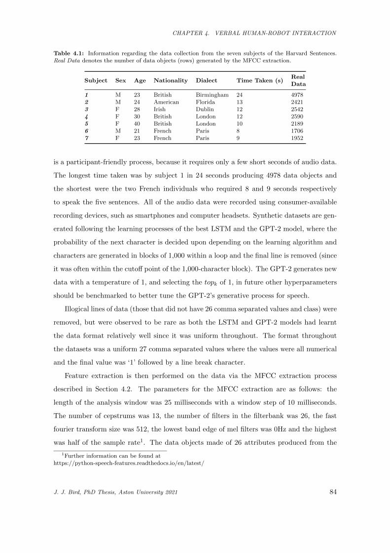
CHAPTER 4. VERBAL HUMAN-ROBOT INTERACTION
Table 4.1: Information regarding the data collection from the seven subjects of the Harvard Sentences.Real Data denotes the number of data objects (rows) generated by the MFCC extraction.
Subject Sex Age Nationality Dialect Time Taken (s)RealData
1 M 23 British Birmingham 24 49782 M 24 American Florida 13 24213 F 28 Irish Dublin 12 25424 F 30 British London 12 25905 F 40 British London 10 21896 M 21 French Paris 8 17067 F 23 French Paris 9 1952
is a participant-friendly process, because it requires only a few short seconds of audio data.
The longest time taken was by subject 1 in 24 seconds producing 4978 data objects and
the shortest were the two French individuals who required 8 and 9 seconds respectively
to speak the five sentences. All of the audio data were recorded using consumer-available
recording devices, such as smartphones and computer headsets. Synthetic datasets are gen-
erated following the learning processes of the best LSTM and the GPT-2 model, where the
probability of the next character is decided upon depending on the learning algorithm and
characters are generated in blocks of 1,000 within a loop and the final line is removed (since
it was often within the cutoff point of the 1,000-character block). The GPT-2 generates new
data with a temperature of 1, and selecting the topk of 1, in future other hyperparameters
should be benchmarked to better tune the GPT-2’s generative process for speech.
Illogical lines of data (those that did not have 26 comma separated values and class) were
removed, but were observed to be rare as both the LSTM and GPT-2 models had learnt
the data format relatively well since it was uniform throughout. The format throughout
the datasets was a uniform 27 comma separated values where the values were all numerical
and the final value was ‘1’ followed by a line break character.
Feature extraction is then performed on the data via the MFCC extraction process
described in Section 4.2. The parameters for the MFCC extraction are as follows: the
length of the analysis window was 25 milliseconds with a window step of 10 milliseconds.
The number of cepstrums was 13, the number of filters in the filterbank was 26, the fast
fourier transform size was 512, the lowest band edge of mel filters was 0Hz and the highest
was half of the sample rate1. The data objects made of 26 attributes produced from the
1Further information can be found athttps://python-speech-features.readthedocs.io/en/latest/
J. J. Bird, PhD Thesis, Aston University 2021 84
CHAPTER 4. VERBAL HUMAN-ROBOT INTERACTION
sliding window are then treated as the input attributes for the neural networks for both
speaker recognition and synthetic data generation (with a class label). This process is
performed on the Flickr8K and Fluent Speech Commands datasets as well as the real data
recorded from the subjects. The MFCC data from each of the 7 subjects’ audio recordings
are used as input to the LSTM and GPT-2 generative models for training and subsequent
data augmentation.
4.3.1.2 Speaker Classification Learning Process
For each subject, the Flickr/FSC data and recorded audio form the basis dataset and
the speaker recognition problem. Eight datasets for transfer learning are then formed on
a per-subject basis, which are the aforementioned data plus 2500, 5000, 7500 and 10000
synthetic data objects generated by either the LSTM or the GPT-2 models. The number
of synthetic data objects are treated as a hyperparameter tuning and selection problem,
since differing numbers of additional synthetic inputs were noted to improve the models, or
cause classification issues compared to the vanilla classification problem. Thus, the models
selected are those that perform best. LSTM has a standard dropout of 0.2 between each
layer. The baseline accuracy for comparison is given as “Synth. Data: 0” later in Table 4.3
which denotes a model that has not been exposed to any of the synthetic data. This baseline
gives scores that are directly comparable to identical networks with their initial weight
distributions being those trained to classify synthetic data generated for the subject, which
is then used to learn from the real data. As previously described, two sets of synthetic data
to expose the models to during pre-training of the real speaker classification problem are
generated by either an LSTM or a GPT-2 language model. Please note that due to this, the
results presented have no baring on whether or not the network could classify the synthetic
data well or otherwise, the weights are simply used as the initial distribution for the same
problem. If the transfer learning networks achieve better results than the networks that
have not been trained on such data, this provides evidence for the hypothesis that speaker
classification can be improved by these methods of data augmentation (See Figure 4.1 for
the process).
An evolutionary search of neural network topologies found that three hidden layers of
30, 7, and 29 neurons were strong for classification of MFCC phoneme classes, and so this
topology is used. The neurons in the layers are all ReLu activation neurons and the network
J. J. Bird, PhD Thesis, Aston University 2021 85
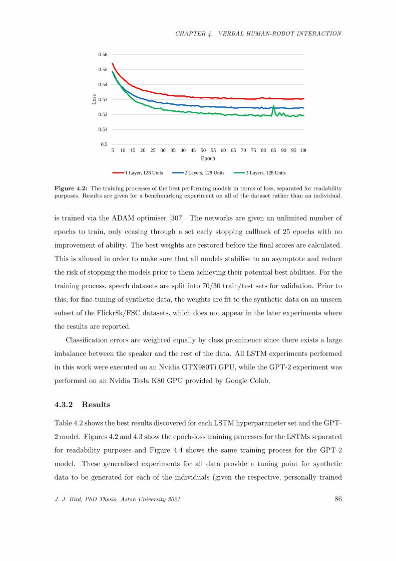
CHAPTER 4. VERBAL HUMAN-ROBOT INTERACTION
0.5
0.51
0.52
0.53
0.54
0.55
0.56
5 10 15 20 25 30 35 40 45 50 55 60 65 70 75 80 85 90 95 100
Loss
Epoch
1 Layer, 128 Units 2 Layers, 128 Units 3 Layers, 128 Units
Figure 4.2: The training processes of the best performing models in terms of loss, separated for readabilitypurposes. Results are given for a benchmarking experiment on all of the dataset rather than an individual.
is trained via the ADAM optimiser [307]. The networks are given an unlimited number of
epochs to train, only ceasing through a set early stopping callback of 25 epochs with no
improvement of ability. The best weights are restored before the final scores are calculated.
This is allowed in order to make sure that all models stabilise to an asymptote and reduce
the risk of stopping the models prior to them achieving their potential best abilities. For the
training process, speech datasets are split into 70/30 train/test sets for validation. Prior to
this, for fine-tuning of synthetic data, the weights are fit to the synthetic data on an unseen
subset of the Flickr8k/FSC datasets, which does not appear in the later experiments where
the results are reported.
Classification errors are weighted equally by class prominence since there exists a large
imbalance between the speaker and the rest of the data. All LSTM experiments performed
in this work were executed on an Nvidia GTX980Ti GPU, while the GPT-2 experiment was
performed on an Nvidia Tesla K80 GPU provided by Google Colab.
4.3.2 Results
Table 4.2 shows the best results discovered for each LSTM hyperparameter set and the GPT-
2 model. Figures 4.2 and 4.3 show the epoch-loss training processes for the LSTMs separated
for readability purposes and Figure 4.4 shows the same training process for the GPT-2
model. These generalised experiments for all data provide a tuning point for synthetic
data to be generated for each of the individuals (given the respective, personally trained
J. J. Bird, PhD Thesis, Aston University 2021 86
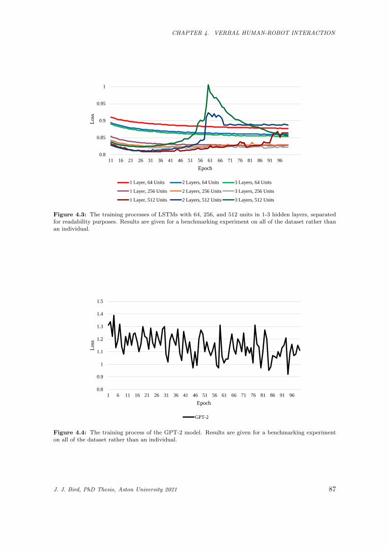
CHAPTER 4. VERBAL HUMAN-ROBOT INTERACTION
0.8
0.85
0.9
0.95
1
11 16 21 26 31 36 41 46 51 56 61 66 71 76 81 86 91 96
Loss
Epoch
1 Layer, 64 Units 2 Layers, 64 Units 3 Layers, 64 Units
1 Layer, 256 Units 2 Layers, 256 Units 3 Layers, 256 Units
1 Layer, 512 Units 2 Layers, 512 Units 3 Layers, 512 Units
Figure 4.3: The training processes of LSTMs with 64, 256, and 512 units in 1-3 hidden layers, separatedfor readability purposes. Results are given for a benchmarking experiment on all of the dataset rather thanan individual.
0.8
0.9
1
1.1
1.2
1.3
1.4
1.5
1 6 11 16 21 26 31 36 41 46 51 56 61 66 71 76 81 86 91 96
Loss
Epoch
GPT-2
Figure 4.4: The training process of the GPT-2 model. Results are given for a benchmarking experimenton all of the dataset rather than an individual.
J. J. Bird, PhD Thesis, Aston University 2021 87
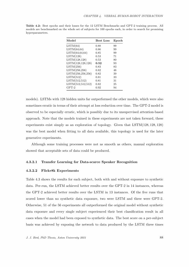
CHAPTER 4. VERBAL HUMAN-ROBOT INTERACTION
Table 4.2: Best epochs and their losses for the 12 LSTM Benchmarks and GPT-2 training process. Allmodels are benchmarked on the whole set of subjects for 100 epochs each, in order to search for promisinghyperparameters.
Model Best Loss Epoch
LSTM(64) 0.88 99LSTM(64,64) 0.86 99LSTM(64,64,64) 0.85 99LSTM(128) 0.53 71LSTM(128,128) 0.53 80LSTM(128,128,128) 0.52 93LSTM(256) 0.83 83LSTM(256,256) 0.82 46LSTM(256,256,256) 0.82 39LSTM(512) 0.81 33LSTM(512,512) 0.81 31LSTM(512,512,512) 0.82 25GPT-2 0.92 94
models). LSTMs with 128 hidden units far outperformed the other models, which were also
sometimes erratic in terms of their attempt at loss reduction over time. The GPT-2 model is
observed to be especially erratic, which is possibly due to its unsupervised attention-based
approach. Note that the models trained in these experiments are not taken forward, these
experiments exist simply as an exploration of topology. Given that LSTM(128, 128, 128)
was the best model when fitting to all data available, this topology is used for the later
generative experiments.
Although some training processes were not as smooth as others, manual exploration
showed that acceptable sets of data could be produced.
4.3.2.1 Transfer Learning for Data-scarce Speaker Recognition
4.3.2.2 Flickr8k Experiments
Table 4.3 shows the results for each subject, both with and without exposure to synthetic
data. Per-run, the LSTM achieved better results over the GPT-2 in 14 instances, whereas
the GPT-2 achieved better results over the LSTM in 13 instances. Of the five runs that
scored lower than no synthetic data exposure, two were LSTM and three were GPT-2.
Otherwise, 51 of the 56 experiments all outperformed the original model without synthetic
data exposure and every single subject experienced their best classification result in all
cases when the model had been exposed to synthetic data. The best score on a per-subject
basis was achieved by exposing the network to data produced by the LSTM three times
J. J. Bird, PhD Thesis, Aston University 2021 88
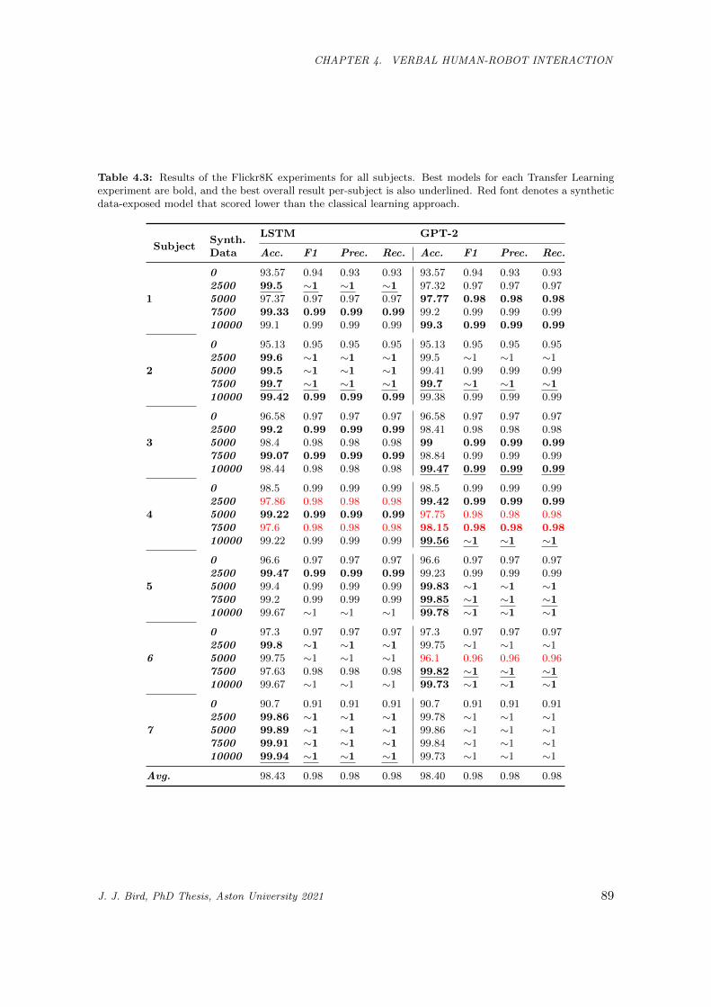
CHAPTER 4. VERBAL HUMAN-ROBOT INTERACTION
Table 4.3: Results of the Flickr8K experiments for all subjects. Best models for each Transfer Learningexperiment are bold, and the best overall result per-subject is also underlined. Red font denotes a syntheticdata-exposed model that scored lower than the classical learning approach.
LSTM GPT-2Subject
Synth.Data Acc. F1 Prec. Rec. Acc. F1 Prec. Rec.
0 93.57 0.94 0.93 0.93 93.57 0.94 0.93 0.932500 99.5 ∼1 ∼1 ∼1 97.32 0.97 0.97 0.975000 97.37 0.97 0.97 0.97 97.77 0.98 0.98 0.987500 99.33 0.99 0.99 0.99 99.2 0.99 0.99 0.99
1
10000 99.1 0.99 0.99 0.99 99.3 0.99 0.99 0.99
0 95.13 0.95 0.95 0.95 95.13 0.95 0.95 0.952500 99.6 ∼1 ∼1 ∼1 99.5 ∼1 ∼1 ∼15000 99.5 ∼1 ∼1 ∼1 99.41 0.99 0.99 0.997500 99.7 ∼1 ∼1 ∼1 99.7 ∼1 ∼1 ∼1
2
10000 99.42 0.99 0.99 0.99 99.38 0.99 0.99 0.99
0 96.58 0.97 0.97 0.97 96.58 0.97 0.97 0.972500 99.2 0.99 0.99 0.99 98.41 0.98 0.98 0.985000 98.4 0.98 0.98 0.98 99 0.99 0.99 0.997500 99.07 0.99 0.99 0.99 98.84 0.99 0.99 0.99
3
10000 98.44 0.98 0.98 0.98 99.47 0.99 0.99 0.99
0 98.5 0.99 0.99 0.99 98.5 0.99 0.99 0.992500 97.86 0.98 0.98 0.98 99.42 0.99 0.99 0.995000 99.22 0.99 0.99 0.99 97.75 0.98 0.98 0.987500 97.6 0.98 0.98 0.98 98.15 0.98 0.98 0.98
4
10000 99.22 0.99 0.99 0.99 99.56 ∼1 ∼1 ∼1
0 96.6 0.97 0.97 0.97 96.6 0.97 0.97 0.972500 99.47 0.99 0.99 0.99 99.23 0.99 0.99 0.995000 99.4 0.99 0.99 0.99 99.83 ∼1 ∼1 ∼17500 99.2 0.99 0.99 0.99 99.85 ∼1 ∼1 ∼1
5
10000 99.67 ∼1 ∼1 ∼1 99.78 ∼1 ∼1 ∼1
0 97.3 0.97 0.97 0.97 97.3 0.97 0.97 0.972500 99.8 ∼1 ∼1 ∼1 99.75 ∼1 ∼1 ∼15000 99.75 ∼1 ∼1 ∼1 96.1 0.96 0.96 0.967500 97.63 0.98 0.98 0.98 99.82 ∼1 ∼1 ∼1
6
10000 99.67 ∼1 ∼1 ∼1 99.73 ∼1 ∼1 ∼1
0 90.7 0.91 0.91 0.91 90.7 0.91 0.91 0.912500 99.86 ∼1 ∼1 ∼1 99.78 ∼1 ∼1 ∼15000 99.89 ∼1 ∼1 ∼1 99.86 ∼1 ∼1 ∼17500 99.91 ∼1 ∼1 ∼1 99.84 ∼1 ∼1 ∼1
7
10000 99.94 ∼1 ∼1 ∼1 99.73 ∼1 ∼1 ∼1
Avg. 98.43 0.98 0.98 0.98 98.40 0.98 0.98 0.98
J. J. Bird, PhD Thesis, Aston University 2021 89
CHAPTER 4. VERBAL HUMAN-ROBOT INTERACTION
and the GPT-2 five times (both including Subject 2 where both were best at 99.7%).
The maximum diversion of training accuracy to validation accuracy was ∼ 1% showing
that although high quality results were attained, overfitting was relatively low; with more
computational resources, k-fold and LOO cross-validation are suggested as future ways to
achieve more accurate measures of variance within classification.
These results show that speaker classification can be improved by exposing the network
to synthetic data produced by both supervised and attention-based models and then trans-
ferring the weights to the initial problem, which most often scores lower without synthetic
data exposure in all cases but five, although those subjects still experienced their absolute
best results through synthetic data exposure regardless.
4.3.2.3 Fluent Speech Commands Experiments
Table 4.4 shows the results for each subject similar to the previous experiment but against
the FSC dataset. In 16 of the experiments, the LSTM achieved the best score as opposed
to the GPT-2 which achieved the best score in 10 of the experiments. During one run of
the LSTM (subject 7, 2500 synthetic data), the score was lower than that of the baseline,
similar issues occurred with the GPT-2 four times with three of those for subject 7. For
the best scores overall, the LSTM achieved the best score five times and the GPT-2 the
other two. The baseline score was always outperformed by a model exposed to a number
of synthetic data. Note that for subject 7, results lower than the vanilla learning process
were higher than that of the models also being exposed to GPT-2 synthetic data. It is
likely that this is due to one of two main reasons; subject 7 produced only a small amount
of data objects in total (1952), and thus the training subset for this subject was smaller
than most others, although on the other hand this did not occur for subject 6 (1706). On
the other hand, since it did not occur in the first experiment, compatibility issues between
subject 7 and the FSC dataset may be the cause. In future planned experiments, large-scale
testing with many subjects using the knowledge gained in this work will aid in exploring
this particular issue.
J. J. Bird, PhD Thesis, Aston University 2021 90
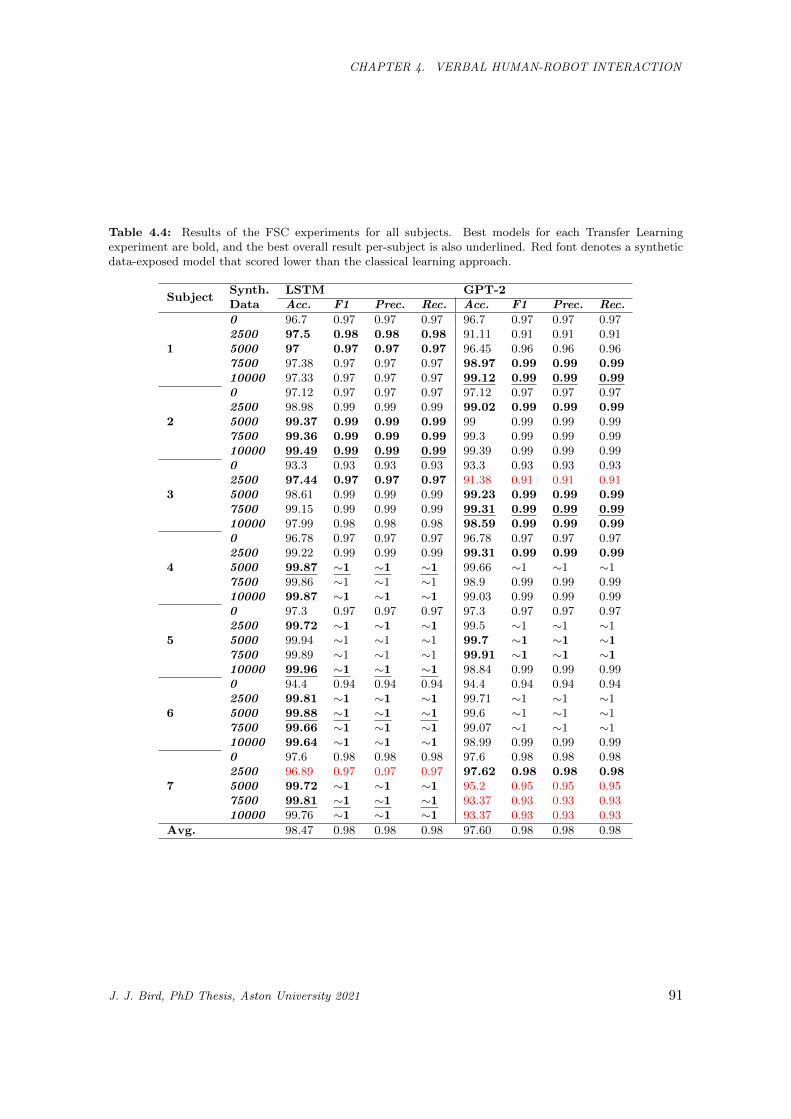
CHAPTER 4. VERBAL HUMAN-ROBOT INTERACTION
Table 4.4: Results of the FSC experiments for all subjects. Best models for each Transfer Learningexperiment are bold, and the best overall result per-subject is also underlined. Red font denotes a syntheticdata-exposed model that scored lower than the classical learning approach.
LSTM GPT-2Subject
Synth.Data Acc. F1 Prec. Rec. Acc. F1 Prec. Rec.
0 96.7 0.97 0.97 0.97 96.7 0.97 0.97 0.972500 97.5 0.98 0.98 0.98 91.11 0.91 0.91 0.915000 97 0.97 0.97 0.97 96.45 0.96 0.96 0.967500 97.38 0.97 0.97 0.97 98.97 0.99 0.99 0.99
1
10000 97.33 0.97 0.97 0.97 99.12 0.99 0.99 0.990 97.12 0.97 0.97 0.97 97.12 0.97 0.97 0.972500 98.98 0.99 0.99 0.99 99.02 0.99 0.99 0.995000 99.37 0.99 0.99 0.99 99 0.99 0.99 0.997500 99.36 0.99 0.99 0.99 99.3 0.99 0.99 0.99
2
10000 99.49 0.99 0.99 0.99 99.39 0.99 0.99 0.990 93.3 0.93 0.93 0.93 93.3 0.93 0.93 0.932500 97.44 0.97 0.97 0.97 91.38 0.91 0.91 0.915000 98.61 0.99 0.99 0.99 99.23 0.99 0.99 0.997500 99.15 0.99 0.99 0.99 99.31 0.99 0.99 0.99
3
10000 97.99 0.98 0.98 0.98 98.59 0.99 0.99 0.990 96.78 0.97 0.97 0.97 96.78 0.97 0.97 0.972500 99.22 0.99 0.99 0.99 99.31 0.99 0.99 0.995000 99.87 ∼1 ∼1 ∼1 99.66 ∼1 ∼1 ∼17500 99.86 ∼1 ∼1 ∼1 98.9 0.99 0.99 0.99
4
10000 99.87 ∼1 ∼1 ∼1 99.03 0.99 0.99 0.990 97.3 0.97 0.97 0.97 97.3 0.97 0.97 0.972500 99.72 ∼1 ∼1 ∼1 99.5 ∼1 ∼1 ∼15000 99.94 ∼1 ∼1 ∼1 99.7 ∼1 ∼1 ∼17500 99.89 ∼1 ∼1 ∼1 99.91 ∼1 ∼1 ∼1
5
10000 99.96 ∼1 ∼1 ∼1 98.84 0.99 0.99 0.990 94.4 0.94 0.94 0.94 94.4 0.94 0.94 0.942500 99.81 ∼1 ∼1 ∼1 99.71 ∼1 ∼1 ∼15000 99.88 ∼1 ∼1 ∼1 99.6 ∼1 ∼1 ∼17500 99.66 ∼1 ∼1 ∼1 99.07 ∼1 ∼1 ∼1
6
10000 99.64 ∼1 ∼1 ∼1 98.99 0.99 0.99 0.990 97.6 0.98 0.98 0.98 97.6 0.98 0.98 0.982500 96.89 0.97 0.97 0.97 97.62 0.98 0.98 0.985000 99.72 ∼1 ∼1 ∼1 95.2 0.95 0.95 0.957500 99.81 ∼1 ∼1 ∼1 93.37 0.93 0.93 0.93
7
10000 99.76 ∼1 ∼1 ∼1 93.37 0.93 0.93 0.93
Avg. 98.47 0.98 0.98 0.98 97.60 0.98 0.98 0.98
J. J. Bird, PhD Thesis, Aston University 2021 91
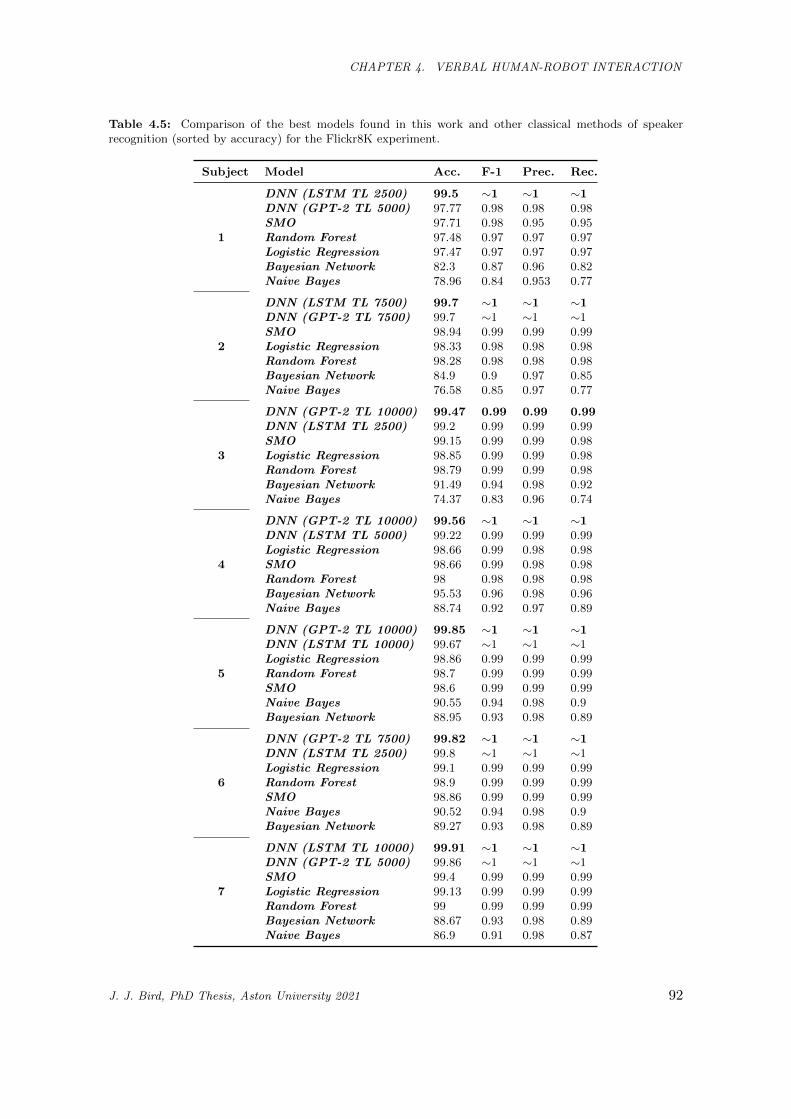
CHAPTER 4. VERBAL HUMAN-ROBOT INTERACTION
Table 4.5: Comparison of the best models found in this work and other classical methods of speakerrecognition (sorted by accuracy) for the Flickr8K experiment.
Subject Model Acc. F-1 Prec. Rec.
1
DNN (LSTM TL 2500) 99.5 ∼1 ∼1 ∼1DNN (GPT-2 TL 5000) 97.77 0.98 0.98 0.98SMO 97.71 0.98 0.95 0.95Random Forest 97.48 0.97 0.97 0.97Logistic Regression 97.47 0.97 0.97 0.97Bayesian Network 82.3 0.87 0.96 0.82Naive Bayes 78.96 0.84 0.953 0.77
2
DNN (LSTM TL 7500) 99.7 ∼1 ∼1 ∼1DNN (GPT-2 TL 7500) 99.7 ∼1 ∼1 ∼1SMO 98.94 0.99 0.99 0.99Logistic Regression 98.33 0.98 0.98 0.98Random Forest 98.28 0.98 0.98 0.98Bayesian Network 84.9 0.9 0.97 0.85Naive Bayes 76.58 0.85 0.97 0.77
3
DNN (GPT-2 TL 10000) 99.47 0.99 0.99 0.99DNN (LSTM TL 2500) 99.2 0.99 0.99 0.99SMO 99.15 0.99 0.99 0.98Logistic Regression 98.85 0.99 0.99 0.98Random Forest 98.79 0.99 0.99 0.98Bayesian Network 91.49 0.94 0.98 0.92Naive Bayes 74.37 0.83 0.96 0.74
4
DNN (GPT-2 TL 10000) 99.56 ∼1 ∼1 ∼1DNN (LSTM TL 5000) 99.22 0.99 0.99 0.99Logistic Regression 98.66 0.99 0.98 0.98SMO 98.66 0.99 0.98 0.98Random Forest 98 0.98 0.98 0.98Bayesian Network 95.53 0.96 0.98 0.96Naive Bayes 88.74 0.92 0.97 0.89
5
DNN (GPT-2 TL 10000) 99.85 ∼1 ∼1 ∼1DNN (LSTM TL 10000) 99.67 ∼1 ∼1 ∼1Logistic Regression 98.86 0.99 0.99 0.99Random Forest 98.7 0.99 0.99 0.99SMO 98.6 0.99 0.99 0.99Naive Bayes 90.55 0.94 0.98 0.9Bayesian Network 88.95 0.93 0.98 0.89
6
DNN (GPT-2 TL 7500) 99.82 ∼1 ∼1 ∼1DNN (LSTM TL 2500) 99.8 ∼1 ∼1 ∼1Logistic Regression 99.1 0.99 0.99 0.99Random Forest 98.9 0.99 0.99 0.99SMO 98.86 0.99 0.99 0.99Naive Bayes 90.52 0.94 0.98 0.9Bayesian Network 89.27 0.93 0.98 0.89
7
DNN (LSTM TL 10000) 99.91 ∼1 ∼1 ∼1DNN (GPT-2 TL 5000) 99.86 ∼1 ∼1 ∼1SMO 99.4 0.99 0.99 0.99Logistic Regression 99.13 0.99 0.99 0.99Random Forest 99 0.99 0.99 0.99Bayesian Network 88.67 0.93 0.98 0.89Naive Bayes 86.9 0.91 0.98 0.87
J. J. Bird, PhD Thesis, Aston University 2021 92
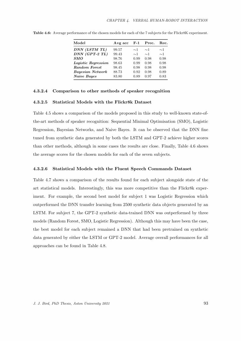
CHAPTER 4. VERBAL HUMAN-ROBOT INTERACTION
Table 4.6: Average performance of the chosen models for each of the 7 subjects for the Flickr8K experiment.
Model Avg acc F-1 Prec. Rec.
DNN (LSTM TL) 99.57 ∼1 ∼1 ∼1DNN (GPT-2 TL) 99.43 ∼1 ∼1 ∼1SMO 98.76 0.99 0.98 0.98Logistic Regression 98.63 0.99 0.98 0.98Random Forest 98.45 0.98 0.98 0.98Bayesian Network 88.73 0.92 0.98 0.89Naive Bayes 83.80 0.89 0.97 0.83
4.3.2.4 Comparison to other methods of speaker recognition
4.3.2.5 Statistical Models with the Flickr8k Dataset
Table 4.5 shows a comparison of the models proposed in this study to well-known state-of-
the-art methods of speaker recognition: Sequential Minimal Optimisation (SMO), Logistic
Regression, Bayesian Networks, and Naive Bayes. It can be observed that the DNN fine
tuned from synthetic data generated by both the LSTM and GPT-2 achieve higher scores
than other methods, although in some cases the results are close. Finally, Table 4.6 shows
the average scores for the chosen models for each of the seven subjects.
4.3.2.6 Statistical Models with the Fluent Speech Commands Dataset
Table 4.7 shows a comparison of the results found for each subject alongside state of the
art statistical models. Interestingly, this was more competitive than the Flickr8k exper-
iment. For example, the second best model for subject 1 was Logistic Regression which
outperformed the DNN transfer learning from 2500 synthetic data objects generated by an
LSTM. For subject 7, the GPT-2 synthetic data-trained DNN was outperformed by three
models (Random Forest, SMO, Logistic Regression). Although this may have been the case,
the best model for each subject remained a DNN that had been pretrained on synthetic
data generated by either the LSTM or GPT-2 model. Average overall performances for all
approaches can be found in Table 4.8.
J. J. Bird, PhD Thesis, Aston University 2021 93
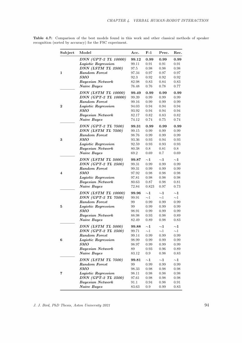
CHAPTER 4. VERBAL HUMAN-ROBOT INTERACTION
Table 4.7: Comparison of the best models found in this work and other classical methods of speakerrecognition (sorted by accuracy) for the FSC experiment.
Subject Model Acc. F-1 Prec. Rec.
1
DNN (GPT-2 TL 10000) 99.12 0.99 0.99 0.99Logistic Regression 99.11 0.91 0.91 0.91DNN (LSTM TL 2500) 97.5 0.98 0.98 0.98Random Forest 97.34 0.97 0.97 0.97SMO 92.3 0.92 0.92 0.92Bayesian Network 82.98 0.83 0.84 0.83Naive Bayes 76.48 0.76 0.78 0.77
2
DNN (LSTM TL 10000) 99.49 0.99 0.99 0.99DNN (GPT-2 TL 10000) 99.39 0.99 0.99 0.99Random Forest 99.16 0.99 0.99 0.99Logistic Regression 94.03 0.94 0.94 0.94SMO 93.92 0.94 0.94 0.94Bayesian Network 82.17 0.82 0.83 0.82Naive Bayes 74.12 0.74 0.75 0.74
3
DNN (GPT-2 TL 7500) 99.31 0.99 0.99 0.99DNN (LSTM TL 7500) 99.15 0.99 0.99 0.99Random Forest 98.76 0.99 0.99 0.99SMO 93.36 0.93 0.94 0.93Logistic Regression 92.59 0.93 0.93 0.93Bayesian Network 80.38 0.8 0.81 0.8Naive Bayes 69.2 0.69 0.7 0.69
4
DNN (LSTM TL 5000) 99.87 ∼1 ∼1 ∼1DNN (GPT-2 TL 2500) 99.31 0.99 0.99 0.99Random Forest 99.31 0.99 0.99 0.99SMO 97.92 0.98 0.98 0.98Logistic Regression 97.81 0.98 0.98 0.98Bayesian Network 80.63 0.87 0.98 0.81Naive Bayes 72.84 0.823 0.97 0.73
5
DNN (LSTM TL 10000) 99.96 ∼1 ∼1 ∼1DNN (GPT-2 TL 7500) 99.91 ∼1 ∼1 ∼1Random Forest 99 0.99 0.99 0.99Logistic Regression 99 0.99 0.99 0.99SMO 98.91 0.99 0.99 0.99Bayesian Network 88.98 0.93 0.98 0.89Naive Bayes 82.49 0.89 0.98 0.83
6
DNN (LSTM TL 5000) 99.88 ∼1 ∼1 ∼1DNN (GPT-2 TL 2500) 99.71 ∼1 ∼1 ∼1Random Forest 99.14 0.99 0.99 0.99Logistic Regression 98.99 0.99 0.99 0.99SMO 98.97 0.99 0.99 0.99Bayesian Network 89 0.93 0.96 0.89Naive Bayes 83.12 0.9 0.98 0.83
7
DNN (LSTM TL 7500) 99.81 ∼1 ∼1 ∼1Random Forest 99 0.99 0.99 0.99SMO 98.33 0.98 0.98 0.98Logistic Regression 98.11 0.98 0.98 0.98DNN (GPT-2 TL 2500) 97.61 0.98 0.98 0.98Bayesian Network 91.1 0.94 0.98 0.91Naive Bayes 83.63 0.9 0.99 0.83
J. J. Bird, PhD Thesis, Aston University 2021 94
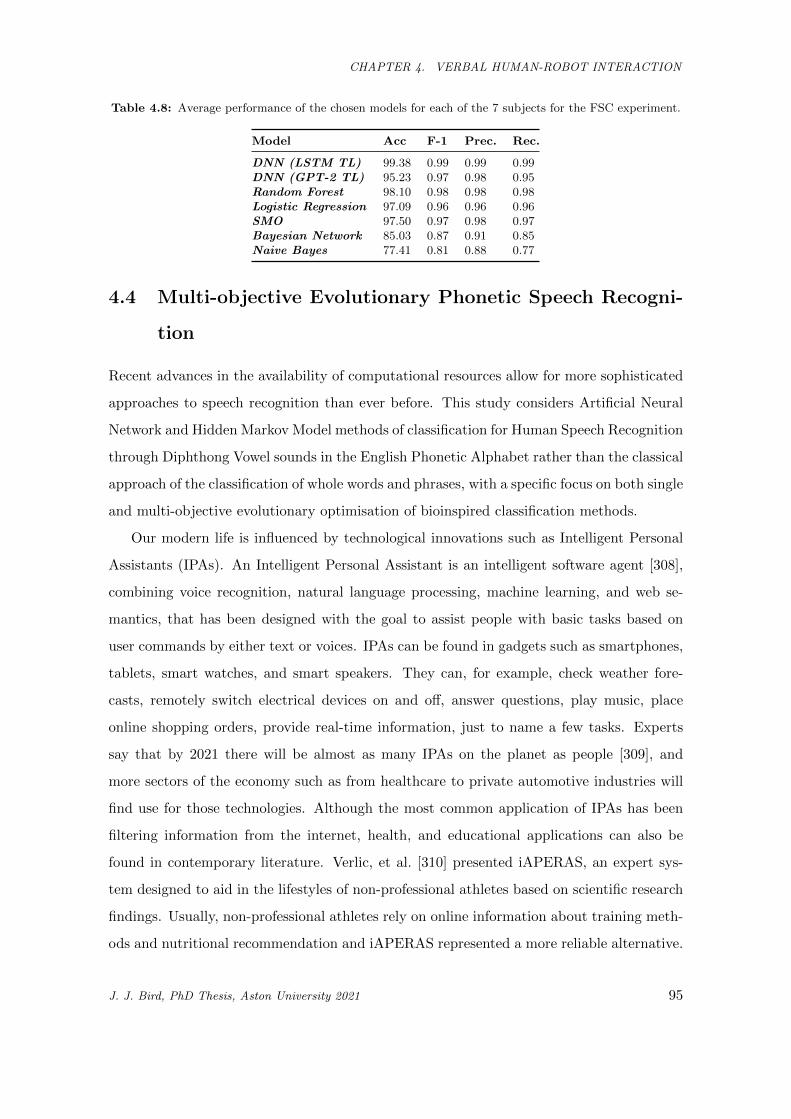
CHAPTER 4. VERBAL HUMAN-ROBOT INTERACTION
Table 4.8: Average performance of the chosen models for each of the 7 subjects for the FSC experiment.
Model Acc F-1 Prec. Rec.
DNN (LSTM TL) 99.38 0.99 0.99 0.99DNN (GPT-2 TL) 95.23 0.97 0.98 0.95Random Forest 98.10 0.98 0.98 0.98Logistic Regression 97.09 0.96 0.96 0.96SMO 97.50 0.97 0.98 0.97Bayesian Network 85.03 0.87 0.91 0.85Naive Bayes 77.41 0.81 0.88 0.77
4.4 Multi-objective Evolutionary Phonetic Speech Recogni-
tion
Recent advances in the availability of computational resources allow for more sophisticated
approaches to speech recognition than ever before. This study considers Artificial Neural
Network and Hidden Markov Model methods of classification for Human Speech Recognition
through Diphthong Vowel sounds in the English Phonetic Alphabet rather than the classical
approach of the classification of whole words and phrases, with a specific focus on both single
and multi-objective evolutionary optimisation of bioinspired classification methods.
Our modern life is influenced by technological innovations such as Intelligent Personal
Assistants (IPAs). An Intelligent Personal Assistant is an intelligent software agent [308],
combining voice recognition, natural language processing, machine learning, and web se-
mantics, that has been designed with the goal to assist people with basic tasks based on
user commands by either text or voices. IPAs can be found in gadgets such as smartphones,
tablets, smart watches, and smart speakers. They can, for example, check weather fore-
casts, remotely switch electrical devices on and off, answer questions, play music, place
online shopping orders, provide real-time information, just to name a few tasks. Experts
say that by 2021 there will be almost as many IPAs on the planet as people [309], and
more sectors of the economy such as from healthcare to private automotive industries will
find use for those technologies. Although the most common application of IPAs has been
filtering information from the internet, health, and educational applications can also be
found in contemporary literature. Verlic, et al. [310] presented iAPERAS, an expert sys-
tem designed to aid in the lifestyles of non-professional athletes based on scientific research
findings. Usually, non-professional athletes rely on online information about training meth-
ods and nutritional recommendation and iAPERAS represented a more reliable alternative.
J. J. Bird, PhD Thesis, Aston University 2021 95
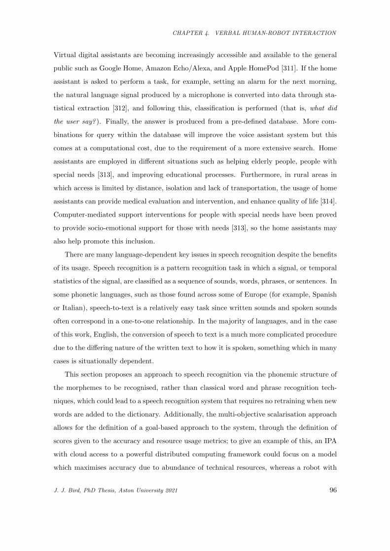
CHAPTER 4. VERBAL HUMAN-ROBOT INTERACTION
Virtual digital assistants are becoming increasingly accessible and available to the general
public such as Google Home, Amazon Echo/Alexa, and Apple HomePod [311]. If the home
assistant is asked to perform a task, for example, setting an alarm for the next morning,
the natural language signal produced by a microphone is converted into data through sta-
tistical extraction [312], and following this, classification is performed (that is, what did
the user say? ). Finally, the answer is produced from a pre-defined database. More com-
binations for query within the database will improve the voice assistant system but this
comes at a computational cost, due to the requirement of a more extensive search. Home
assistants are employed in different situations such as helping elderly people, people with
special needs [313], and improving educational processes. Furthermore, in rural areas in
which access is limited by distance, isolation and lack of transportation, the usage of home
assistants can provide medical evaluation and intervention, and enhance quality of life [314].
Computer-mediated support interventions for people with special needs have been proved
to provide socio-emotional support for those with needs [313], so the home assistants may
also help promote this inclusion.
There are many language-dependent key issues in speech recognition despite the benefits
of its usage. Speech recognition is a pattern recognition task in which a signal, or temporal
statistics of the signal, are classified as a sequence of sounds, words, phrases, or sentences. In
some phonetic languages, such as those found across some of Europe (for example, Spanish
or Italian), speech-to-text is a relatively easy task since written sounds and spoken sounds
often correspond in a one-to-one relationship. In the majority of languages, and in the case
of this work, English, the conversion of speech to text is a much more complicated procedure
due to the differing nature of the written text to how it is spoken, something which in many
cases is situationally dependent.
This section proposes an approach to speech recognition via the phonemic structure of
the morphemes to be recognised, rather than classical word and phrase recognition tech-
niques, which could lead to a speech recognition system that requires no retraining when new
words are added to the dictionary. Additionally, the multi-objective scalarisation approach
allows for the definition of a goal-based approach to the system, through the definition of
scores given to the accuracy and resource usage metrics; to give an example of this, an IPA
with cloud access to a powerful distributed computing framework could focus on a model
which maximises accuracy due to abundance of technical resources, whereas a robot with
J. J. Bird, PhD Thesis, Aston University 2021 96
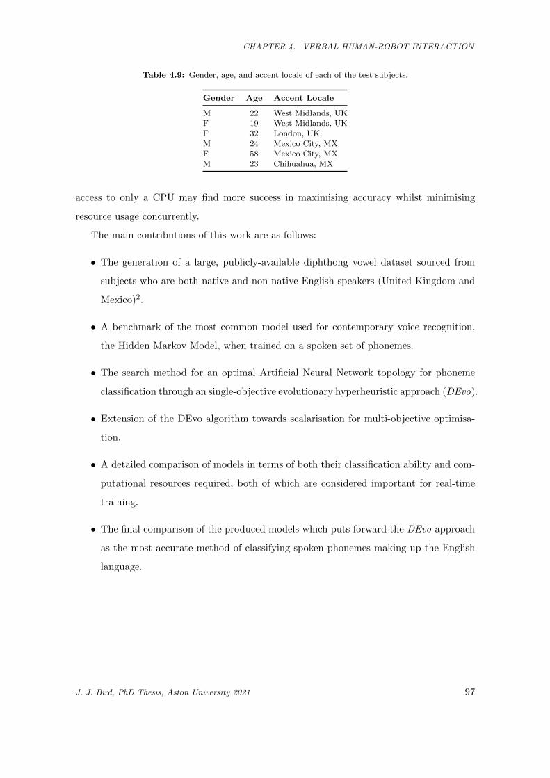
CHAPTER 4. VERBAL HUMAN-ROBOT INTERACTION
Table 4.9: Gender, age, and accent locale of each of the test subjects.
Gender Age Accent Locale
M 22 West Midlands, UKF 19 West Midlands, UKF 32 London, UKM 24 Mexico City, MXF 58 Mexico City, MXM 23 Chihuahua, MX
access to only a CPU may find more success in maximising accuracy whilst minimising
resource usage concurrently.
The main contributions of this work are as follows:
• The generation of a large, publicly-available diphthong vowel dataset sourced from
subjects who are both native and non-native English speakers (United Kingdom and
Mexico)2.
• A benchmark of the most common model used for contemporary voice recognition,
the Hidden Markov Model, when trained on a spoken set of phonemes.
• The search method for an optimal Artificial Neural Network topology for phoneme
classification through an single-objective evolutionary hyperheuristic approach (DEvo).
• Extension of the DEvo algorithm towards scalarisation for multi-objective optimisa-
tion.
• A detailed comparison of models in terms of both their classification ability and com-
putational resources required, both of which are considered important for real-time
training.
• The final comparison of the produced models which puts forward the DEvo approach
as the most accurate method of classifying spoken phonemes making up the English
language.
J. J. Bird, PhD Thesis, Aston University 2021 97
CHAPTER 4. VERBAL HUMAN-ROBOT INTERACTION
Phoneme 1
Phoneme 2
Phoneme 3
Phoneme n
...
MFCC
FeatureExtraction
TrainedModel
UnknownPhoneme
FeatureExtraction
MFCC
Prediction
Figure 4.5: Description of the training and prediction process applied in this study. Initial training happensto the left of the trained model where phonemes are used as data objects for learning and validated through10-fold cross-validation; prediction of unknown phonemes from sound data occurs to the right of the model.
4.4.1 Method
4.4.1.1 Data Collection and Attribute Generation
For recording an audio dataset, subjects were all asked to pronounce the sound as if they
were speaking English although not all of the subjects were native English speakers. All of
the seven diphthong vowel sounds were recorded ten times each by the six subjects as can be
seen in Table 4.9. The three subjects from the United Kingdom are native English speakers,
whereas the Mexican subjects were native Spanish speakers but had a fluent proficiency in
English. The resultant dataset of 420 individual sound clips were processed in order to
remove silence and then produce an MFCC dataset by a sliding a window of length 200ms.
Ultimately, this produced a large dataset of 32,398 data objects for classification.
4.4.1.2 Machine Learning
The training and prediction process applied in this study can be summarised in Figure 4.5.
Input parameters are considered to be the set of recorded phonemes to train the selected
model. Data is converted to a relational time-series for HMM, whereas data is randomised
for the MLP. A dataset is then generated from the phonemes recorded via statistical ex-
traction by way of their Mel-frequency Cepstral Coefficients, which are then normalised.
Machine learning models are trained and validated using 10-fold cross validation, and mea-
sured by their overall accuracy. The solution MLPs are given a standard 500 epochs of
training time, learning rate of 0.3, and a momentum of 0.2 which were chosen manually
based on initial exploration. Future work outlines the further optimisation of these param-
eters. The chosen approach for the optimisation of ANN topology is the DEvo approach
2https://www.kaggle.com/birdy654/speech-recognition-dataset-england-and-mexico
J. J. Bird, PhD Thesis, Aston University 2021 98
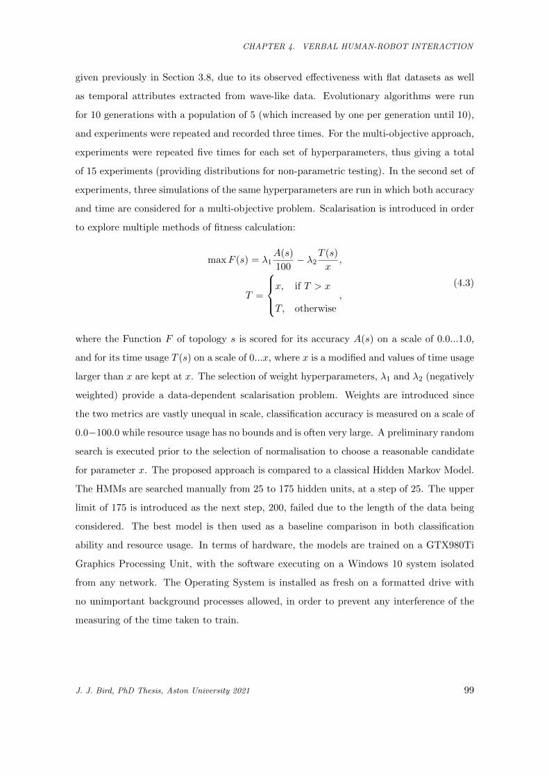
CHAPTER 4. VERBAL HUMAN-ROBOT INTERACTION
given previously in Section 3.8, due to its observed effectiveness with flat datasets as well
as temporal attributes extracted from wave-like data. Evolutionary algorithms were run
for 10 generations with a population of 5 (which increased by one per generation until 10),
and experiments were repeated and recorded three times. For the multi-objective approach,
experiments were repeated five times for each set of hyperparameters, thus giving a total
of 15 experiments (providing distributions for non-parametric testing). In the second set of
experiments, three simulations of the same hyperparameters are run in which both accuracy
and time are considered for a multi-objective problem. Scalarisation is introduced in order
to explore multiple methods of fitness calculation:
maxF (s) = λ1A(s)
100− λ2
T (s)
x,
T =
⎧⎪⎨⎪⎩x, if T > x
T, otherwise
,(4.3)
where the Function F of topology s is scored for its accuracy A(s) on a scale of 0.0...1.0,
and for its time usage T (s) on a scale of 0...x, where x is a modified and values of time usage
larger than x are kept at x. The selection of weight hyperparameters, λ1 and λ2 (negatively
weighted) provide a data-dependent scalarisation problem. Weights are introduced since
the two metrics are vastly unequal in scale, classification accuracy is measured on a scale of
0.0−100.0 while resource usage has no bounds and is often very large. A preliminary random
search is executed prior to the selection of normalisation to choose a reasonable candidate
for parameter x. The proposed approach is compared to a classical Hidden Markov Model.
The HMMs are searched manually from 25 to 175 hidden units, at a step of 25. The upper
limit of 175 is introduced as the next step, 200, failed due to the length of the data being
considered. The best model is then used as a baseline comparison in both classification
ability and resource usage. In terms of hardware, the models are trained on a GTX980Ti
Graphics Processing Unit, with the software executing on a Windows 10 system isolated
from any network. The Operating System is installed as fresh on a formatted drive with
no unimportant background processes allowed, in order to prevent any interference of the
measuring of the time taken to train.
J. J. Bird, PhD Thesis, Aston University 2021 99
CHAPTER 4. VERBAL HUMAN-ROBOT INTERACTION
25 50 75 100 125 150 17580
82
84
86
88
HMM Hidden Units
Classification
Accuracy
(%)
HMM Accuracy
Figure 4.6: Benchmarking of HMM hidden units.
4.4.2 Results
4.4.2.1 HMM Topology Selection
For choosing the best HMM topology, an approach of manual exploration was applied. Hid-
den Markov Models comprised of a topology of 25 to 175 hidden units were tested, at a step
of 25, and were used to attempt to classify the whole dataset. Figure 4.6 shows the accuracy
of the phoneme classification for each HMM tested. Results showed the HMM having 150
hidden units provided the best accuracy result (86.23%) for phoneme classification on this
dataset. This model was then used as a baseline for comparison to the proposed approach.
200 Hidden Units extended beyond the majority of data series and thus the model could
not be trained without error, therefore, 175 was the upper limit for benchmarking.
4.4.2.2 Single Objective Optimisation of Accuracy
When performing an evolutionary search of the Neural Network topology, the decision
variables were the number of hidden layers ([1, 5]) and number of neurons in each hidden
layer ([1, 100]). In the single-objective optimisation, the accuracy was the function to be
maximised. Table 4.10 shows the best accuracy of the strongest neural net solution at each
generation of the evolutionary search. Due to the complexity of the search in comparison to
the resources available, a relatively limited search was performed but with success. The best
results for each search are shown in 4.10. Their differing areas of the search space suggest
J. J. Bird, PhD Thesis, Aston University 2021 100
CHAPTER 4. VERBAL HUMAN-ROBOT INTERACTION
that an optimal solution is being converged upon rather than local minima. With more
resources available, a more thorough search should be performed in an attempt to derive
an even more effective ANN topology than the three layer network suggested. It is possible
to see that an MLP with hyper-heuristically optimised topology has a high classification
ability (88.84%) when it comes to the MFCC time windows of audio data in terms of spoken
phonemes by both native and non-native English speakers when compared to a classical
HMM (86.23%). The advantage of the optimised deep network over the HMM is greater
than 2% in terms of simply accuracy alone. If efficiency in terms of time is also of concern,
the computational resources required by each of the models for training can be observed in
Figure 4.8. The time spent in 10-fold Cross validation was measured for each final ANN
topology, for each simulation run for the evolutionary approach, and for the HMM. The
best model found was S4 but it had the highest training time of 248.76. It can be observed
that single layer models were competitive but took far fewer computational resources to
train; Solution S1 was the weakest suggestion by the evolutionary approach, and yet still
outperformed the best HMM by 1.27% in terms of accuracy while training in less time,
a successful reduction of 4.09 seconds compared to the Hidden Markov Model. Although
this relatively short decrease in time is observed, an IoT device such as an autonomous
robot with access to only a CPU rather than a GPU would experience a far bigger resource
advantage. Note that when the number of layers increases from one to three, the accuracy
increases from 88.3% to 88.84% and time spent also increases from 180.34 seconds to 232.9
seconds. Also, comparing the obtained ANN with only one layers, layer size seems more
important than depth. One important question that arises is the advantage of deep networks
for the phoneme recognition problem using this dataset and thus, exploration of only one
hidden layer of size n neurons was performed through the subsequent three simulations.
Detailed results from this simulation (S4) are shown in Figure 4.7 where a single layer of
57 neurons gave the best result of 90.77% at a cost of 248.76 seconds in training time, by
far the most computationally complex model produced.
J. J. Bird, PhD Thesis, Aston University 2021 101
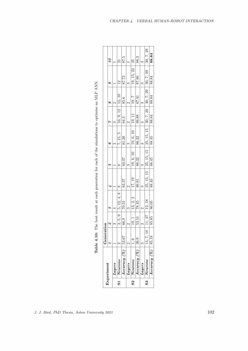
CHAPTER 4. VERBAL HUMAN-ROBOT INTERACTION
Table
4.10:
Th
eb
est
resu
ltat
each
gen
erati
on
for
each
of
the
sim
ula
tion
sto
op
tim
ise
an
ML
PA
NN
.
Experiment
Genera
tion
12
34
56
78
910
S1
Layers
13
41
13
32
11
Neuro
ns
23,
5,
95,
12,
4,
88
87,
15,
510,
9,
12
12,
10
12
21
Acc
ura
cy(%
)53.6
766.9
70.3
183.3
783.3
781.2
684.3
85.6
87.7
387.5
S2
Layers
22
32
33
22
31
Neuro
ns
1,
619,
113,
2,
217,
19
19,
6,
10
19,
6,
10
19,
11
19,
719,
15,
22
25
Acc
ura
cy(%
)36.9
53.5
178.4
586.8
186.3
286.3
286.8
887.4
187.8
688.3
S3
Layers
32
23
33
33
33
Neuro
ns
14,
7,
18
11,
27
12,
18
25,
15,
15
25,
15,
15
25,
15,
15
30,
7,
29
30,
7,
29
30,
7,
29
30,
7,
29
Acc
ura
cy(%
)85.1
885.8
586.0
588.4
588.4
588.4
588.8
488.8
488.8
488.84
J. J. Bird, PhD Thesis, Aston University 2021 102
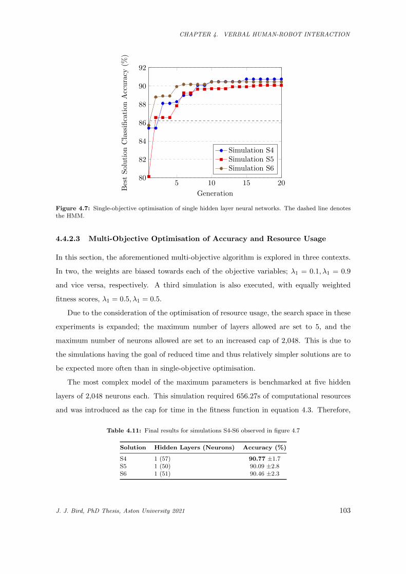
CHAPTER 4. VERBAL HUMAN-ROBOT INTERACTION
5 10 15 2080
82
84
86
88
90
92
Generation
BestSolutionClassification
Accuracy
(%)
Simulation S4Simulation S5Simulation S6
Figure 4.7: Single-objective optimisation of single hidden layer neural networks. The dashed line denotesthe HMM.
4.4.2.3 Multi-Objective Optimisation of Accuracy and Resource Usage
In this section, the aforementioned multi-objective algorithm is explored in three contexts.
In two, the weights are biased towards each of the objective variables; λ1 = 0.1, λ1 = 0.9
and vice versa, respectively. A third simulation is also executed, with equally weighted
fitness scores, λ1 = 0.5, λ1 = 0.5.
Due to the consideration of the optimisation of resource usage, the search space in these
experiments is expanded; the maximum number of layers allowed are set to 5, and the
maximum number of neurons allowed are set to an increased cap of 2,048. This is due to
the simulations having the goal of reduced time and thus relatively simpler solutions are to
be expected more often than in single-objective optimisation.
The most complex model of the maximum parameters is benchmarked at five hidden
layers of 2,048 neurons each. This simulation required 656.27s of computational resources
and was introduced as the cap for time in the fitness function in equation 4.3. Therefore,
Table 4.11: Final results for simulations S4-S6 observed in figure 4.7
Solution Hidden Layers (Neurons) Accuracy (%)
S4 1 (57) 90.77 ±1.7S5 1 (50) 90.09 ±2.8S6 1 (51) 90.46 ±2.3
J. J. Bird, PhD Thesis, Aston University 2021 103
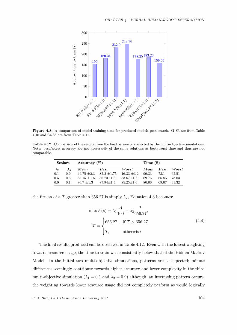
CHAPTER 4. VERBAL HUMAN-ROBOT INTERACTION
S1(8
7.5%±2.
3)
S2(8
8.3%±1.
1)
S3(8
8.84
%±1.
6)
HM
M(8
6.23
%±1.
7)
S4(9
0.77
%±1.
7)
S5(9
0.09
%±2.
8)
S6(9
0.46
%±2.
3)0
50
100
150
200
250
300
155
180.34
232.9
159.09
248.76
178.25 183.23
Ap
pro
x.
tim
eto
train
(s)
Figure 4.8: A comparison of model training time for produced models post-search. S1-S3 are from Table4.10 and S4-S6 are from Table 4.11.
Table 4.12: Comparison of the results from the final parameters selected by the multi-objective simulations.Note: best/worst accuracy are not necessarily of the same solutions as best/worst time and thus are notcomparable.
Scalars Accuracy (%) Time (S)
λ1 λ2 Mean Best Worst Mean Best Worst0.1 0.9 49.75 ±2.3 82.2 ±1.75 16.33 ±3.2 99.33 73.1 62.510.5 0.5 85.15 ±1.6 86.73±1.6 83.67±1.6 69.75 66.85 73.030.9 0.1 86.7 ±1.3 87.94±1.4 85.25±1.6 80.66 69.07 91.32
the fitness of a T greater than 656.27 is simply λ2, Equation 4.3 becomes:
maxF (s) = λ1A
100− λ2
T
656.27,
T =
⎧⎪⎨⎪⎩656.27, if T > 656.27
T, otherwise
(4.4)
The final results produced can be observed in Table 4.12. Even with the lowest weighting
towards resource usage, the time to train was consistently below that of the Hidden Markov
Model. In the initial two multi-objective simulations, patterns are as expected; minute
differences seemingly contribute towards higher accuracy and lower complexity.In the third
multi-objective simulation (λ1 = 0.1 and λ2 = 0.9) although, an interesting pattern occurs;
the weighting towards lower resource usage did not completely perform as would logically
J. J. Bird, PhD Thesis, Aston University 2021 104
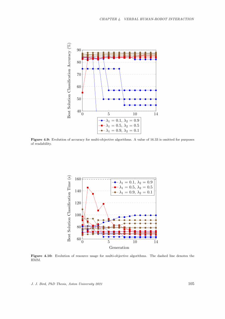
CHAPTER 4. VERBAL HUMAN-ROBOT INTERACTION
0 5 10 1440
50
60
70
80
90
Generation
BestSolution
ClassificationAccuracy
(%)
λ1 = 0.1, λ2 = 0.9λ1 = 0.5, λ2 = 0.5λ1 = 0.9, λ2 = 0.1
Figure 4.9: Evolution of accuracy for multi-objective algorithms. A value of 16.33 is omitted for purposesof readability.
0 5 10 1460
80
100
120
140
160
Generation
BestSolutionClassificationTim
e(s)
λ1 = 0.1, λ2 = 0.9λ1 = 0.5, λ2 = 0.5λ1 = 0.9, λ2 = 0.1
Figure 4.10: Evolution of resource usage for multi-objective algorithms. The dashed line denotes theHMM.
J. J. Bird, PhD Thesis, Aston University 2021 105
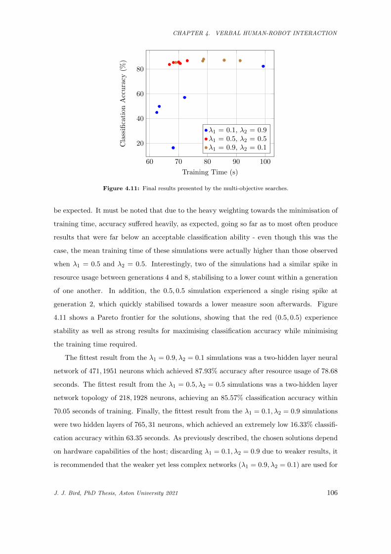
CHAPTER 4. VERBAL HUMAN-ROBOT INTERACTION
60 70 80 90 100
20
40
60
80
Training Time (s)
Classification
Accuracy
(%)
λ1 = 0.1, λ2 = 0.9λ1 = 0.5, λ2 = 0.5λ1 = 0.9, λ2 = 0.1
Figure 4.11: Final results presented by the multi-objective searches.
be expected. It must be noted that due to the heavy weighting towards the minimisation of
training time, accuracy suffered heavily, as expected, going so far as to most often produce
results that were far below an acceptable classification ability - even though this was the
case, the mean training time of these simulations were actually higher than those observed
when λ1 = 0.5 and λ2 = 0.5. Interestingly, two of the simulations had a similar spike in
resource usage between generations 4 and 8, stabilising to a lower count within a generation
of one another. In addition, the 0.5, 0.5 simulation experienced a single rising spike at
generation 2, which quickly stabilised towards a lower measure soon afterwards. Figure
4.11 shows a Pareto frontier for the solutions, showing that the red (0.5, 0.5) experience
stability as well as strong results for maximising classification accuracy while minimising
the training time required.
The fittest result from the λ1 = 0.9, λ2 = 0.1 simulations was a two-hidden layer neural
network of 471, 1951 neurons which achieved 87.93% accuracy after resource usage of 78.68
seconds. The fittest result from the λ1 = 0.5, λ2 = 0.5 simulations was a two-hidden layer
network topology of 218, 1928 neurons, achieving an 85.57% classification accuracy within
70.05 seconds of training. Finally, the fittest result from the λ1 = 0.1, λ2 = 0.9 simulations
were two hidden layers of 765, 31 neurons, which achieved an extremely low 16.33% classifi-
cation accuracy within 63.35 seconds. As previously described, the chosen solutions depend
on hardware capabilities of the host; discarding λ1 = 0.1, λ2 = 0.9 due to weaker results, it
is recommended that the weaker yet less complex networks (λ1 = 0.9, λ2 = 0.1) are used for
J. J. Bird, PhD Thesis, Aston University 2021 106
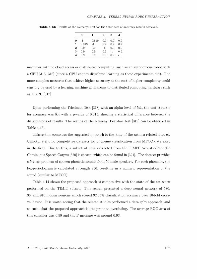
CHAPTER 4. VERBAL HUMAN-ROBOT INTERACTION
Table 4.13: Results of the Nemenyi Test for the three sets of accuracy results achieved.
0 1 2 3 4
0 -1 0.819 0.9 0.9 0.91 0.819 -1 0.9 0.9 0.92 0.9 0.9 -1 0.9 0.93 0.9 0.9 0.9 -1 0.94 0.9 0.9 0.9 0.9 -1
machines with no cloud access or distributed computing, such as an autonomous robot with
a CPU [315, 316] (since a CPU cannot distribute learning as these experiments did). The
more complex networks that achieve higher accuracy at the cost of higher complexity could
sensibly be used by a learning machine with access to distributed computing hardware such
as a GPU [317].
Upon performing the Friedman Test [318] with an alpha level of 5%, the test statistic
for accuracy was 8.4 with a p-value of 0.015, showing a statistical difference between the
distributions of results. The results of the Nemenyi Post-hoc test [319] can be observed in
Table 4.13.
This section compares the suggested approach to the state-of-the-art in a related dataset.
Unfortunately, no competitive datasets for phoneme classification from MFCC data exist
in the field. Due to this, a subset of data extracted from the TIMIT Acoustic-Phonetic
Continuous Speech Corpus [320] is chosen, which can be found in [321]. The dataset provides
a 5-class problem of spoken phonetic sounds from 50 male speakers. For each phoneme, the
log-periodogram is calculated at length 256, resulting in a numeric representation of the
sound (similar to MFCC).
Table 4.14 shows the proposed approach is competitive with the state of the art when
performed on the TIMIT subset. This search presented a deep neural network of 580,
36, and 910 hidden neurons which scored 92.85% classification accuracy over 10-fold cross-
validation. It is worth noting that the related studies performed a data split approach, and
as such, that the proposed approach is less prone to overfitting. The average ROC area of
this classifier was 0.99 and the F-measure was around 0.93.
J. J. Bird, PhD Thesis, Aston University 2021 107
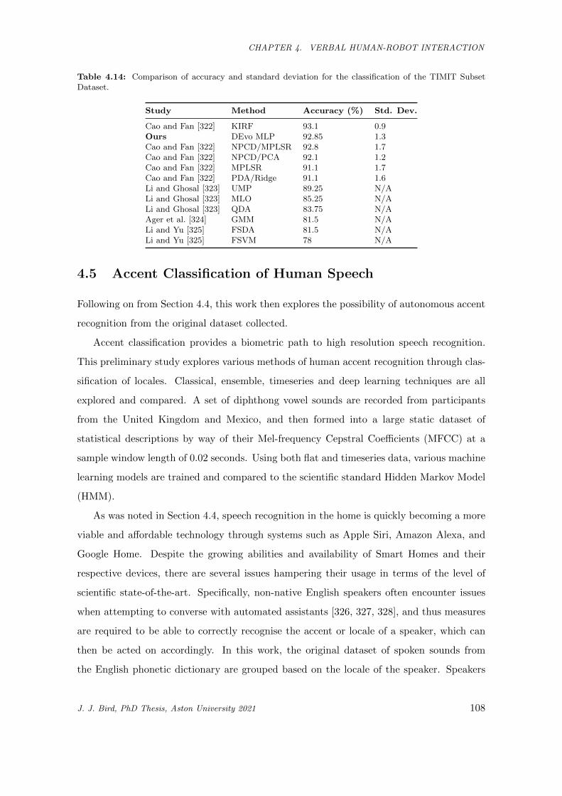
CHAPTER 4. VERBAL HUMAN-ROBOT INTERACTION
Table 4.14: Comparison of accuracy and standard deviation for the classification of the TIMIT SubsetDataset.
Study Method Accuracy (%) Std. Dev.
Cao and Fan [322] KIRF 93.1 0.9Ours DEvo MLP 92.85 1.3Cao and Fan [322] NPCD/MPLSR 92.8 1.7Cao and Fan [322] NPCD/PCA 92.1 1.2Cao and Fan [322] MPLSR 91.1 1.7Cao and Fan [322] PDA/Ridge 91.1 1.6Li and Ghosal [323] UMP 89.25 N/ALi and Ghosal [323] MLO 85.25 N/ALi and Ghosal [323] QDA 83.75 N/AAger et al. [324] GMM 81.5 N/ALi and Yu [325] FSDA 81.5 N/ALi and Yu [325] FSVM 78 N/A
4.5 Accent Classification of Human Speech
Following on from Section 4.4, this work then explores the possibility of autonomous accent
recognition from the original dataset collected.
Accent classification provides a biometric path to high resolution speech recognition.
This preliminary study explores various methods of human accent recognition through clas-
sification of locales. Classical, ensemble, timeseries and deep learning techniques are all
explored and compared. A set of diphthong vowel sounds are recorded from participants
from the United Kingdom and Mexico, and then formed into a large static dataset of
statistical descriptions by way of their Mel-frequency Cepstral Coefficients (MFCC) at a
sample window length of 0.02 seconds. Using both flat and timeseries data, various machine
learning models are trained and compared to the scientific standard Hidden Markov Model
(HMM).
As was noted in Section 4.4, speech recognition in the home is quickly becoming a more
viable and affordable technology through systems such as Apple Siri, Amazon Alexa, and
Google Home. Despite the growing abilities and availability of Smart Homes and their
respective devices, there are several issues hampering their usage in terms of the level of
scientific state-of-the-art. Specifically, non-native English speakers often encounter issues
when attempting to converse with automated assistants [326, 327, 328], and thus measures
are required to be able to correctly recognise the accent or locale of a speaker, which can
then be acted on accordingly. In this work, the original dataset of spoken sounds from
the English phonetic dictionary are grouped based on the locale of the speaker. Speakers
J. J. Bird, PhD Thesis, Aston University 2021 108

CHAPTER 4. VERBAL HUMAN-ROBOT INTERACTION
2 4 6 8 10 12 14 16 18 20 22 24 260.1
0.2
0.3
0.4
0.5
0.6
0.7
0.8
MFCC Log
Inform
ationGain
Figure 4.12: Information Gain of each MFCC log attribute in the dataset.
are both native (West Midlands, UK; London, UK) and non-native (Mexico City, MX;
Chihuahua, MX) English speakers producing a four-class problem. Various single, ensemble
and deep learning models are trained and compared in terms of their classification ability
for accent recognition. A flat dataset of 26 200ms Mel-frequency Cepstral Coefficients form
data objects for classification, except for a timeseries of the aforementioned datapoints that
are generated for Hidden Markov Model training and prediction.
The main contributions of this extension are as follows:
• A benchmark of the most common model used for contemporary voice recognition,
the Hidden Markov Model, when training on a uniform spoken audio dataset and
producing predictions of speaker accent/locale.
• Single and ensemble models are presented for the classification of the accent of two
Mexican locales and two British locales.
• The final comparison of the eleven machine learning models in which a vote of average
probabilities of Random Forest and LSTM is suggested as the best model with a high
classification accuracy of 94.74%.
4.5.1 Method
As previously described, the voice recognition dataset contained seven individual phonetic
sounds spoken ten times each by subjects from the United Kingdom and Mexico. Those
J. J. Bird, PhD Thesis, Aston University 2021 109
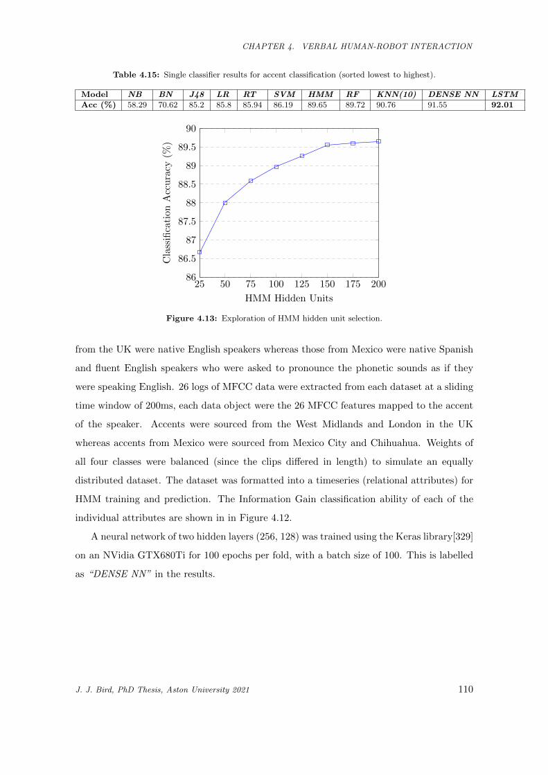
CHAPTER 4. VERBAL HUMAN-ROBOT INTERACTION
Table 4.15: Single classifier results for accent classification (sorted lowest to highest).
Model NB BN J48 LR RT SVM HMM RF KNN(10) DENSE NN LSTM
Acc (%) 58.29 70.62 85.2 85.8 85.94 86.19 89.65 89.72 90.76 91.55 92.01
25 50 75 100 125 150 175 20086
86.5
87
87.5
88
88.5
89
89.5
90
HMM Hidden Units
Classification
Accuracy
(%)
Figure 4.13: Exploration of HMM hidden unit selection.
from the UK were native English speakers whereas those from Mexico were native Spanish
and fluent English speakers who were asked to pronounce the phonetic sounds as if they
were speaking English. 26 logs of MFCC data were extracted from each dataset at a sliding
time window of 200ms, each data object were the 26 MFCC features mapped to the accent
of the speaker. Accents were sourced from the West Midlands and London in the UK
whereas accents from Mexico were sourced from Mexico City and Chihuahua. Weights of
all four classes were balanced (since the clips differed in length) to simulate an equally
distributed dataset. The dataset was formatted into a timeseries (relational attributes) for
HMM training and prediction. The Information Gain classification ability of each of the
individual attributes are shown in in Figure 4.12.
A neural network of two hidden layers (256, 128) was trained using the Keras library[329]
on an NVidia GTX680Ti for 100 epochs per fold, with a batch size of 100. This is labelled
as “DENSE NN” in the results.
J. J. Bird, PhD Thesis, Aston University 2021 110
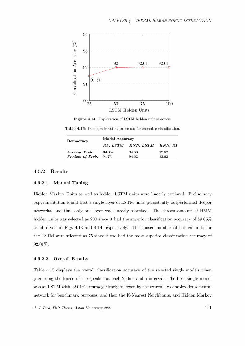
CHAPTER 4. VERBAL HUMAN-ROBOT INTERACTION
25 50 75 10090
91
92
93
94
91.51
92 92.01 92.01
LSTM Hidden Units
Classification
Accuracy
(%)
Figure 4.14: Exploration of LSTM hidden unit selection.
Table 4.16: Democratic voting processes for ensemble classification.
DemocracyModel Accuracy
RF, LSTM KNN, LSTM KNN, RF
Average Prob. 94.74 94.63 92.62Product of Prob. 94.73 94.62 92.62
4.5.2 Results
4.5.2.1 Manual Tuning
Hidden Markov Units as well as hidden LSTM units were linearly explored. Preliminary
experimentation found that a single layer of LSTM units persistently outperformed deeper
networks, and thus only one layer was linearly searched. The chosen amount of HMM
hidden units was selected as 200 since it had the superior classification accuracy of 89.65%
as observed in Figs 4.13 and 4.14 respectively. The chosen number of hidden units for
the LSTM were selected as 75 since it too had the most superior classification accuracy of
92.01%.
4.5.2.2 Overall Results
Table 4.15 displays the overall classification accuracy of the selected single models when
predicting the locale of the speaker at each 200ms audio interval. The best single model
was an LSTM with 92.01% accuracy, closely followed by the extremely complex dense neural
network for benchmark purposes, and then the K-Nearest Neighbours, and Hidden Markov
J. J. Bird, PhD Thesis, Aston University 2021 111
CHAPTER 4. VERBAL HUMAN-ROBOT INTERACTION
Models.
The best ensemble, and the overall best, was a vote of average probability between the
Random Forest and LSTM, achieving 94.74% accuracy, this can be seen in the exploration
of democratic voting processes with the best models, in Table 4.16.
4.6 Phonetic Speech Synthesis
In Sections 4.4 and 4.5, it was discovered that phonemes hold speech recognition ability as
well as classification of the accent spoken, respectively. Following these findings, the work
in this section explores a comparison of raw text and phoneme representation for speech
synthesis. The models themselves were not released given that they could be used to imitate
the author with potential consequences due to the produced speech sounding relatively
realistic, but a demonstration is available at http://jordanjamesbird.com/tacotron/
tacotrontest.html. Artificial Intelligence researchers often seek the goal of intelligent
human imitation. As was discussed within the introduction; in 1950 Alan Turing proposed
the Turing Test, or as he famously called it, the ‘Imitation Game’ [4]. In the seven decades
since, Computer Scientists continue to seek improved methods of true imitation of the multi-
faceted human nature. In this section, the experiments explore a new method towards the
imitation of human speech in terms of audio. In this competition of two differing data
representation methods, rather than a human judge, statistical analyses work to distinguish
the differences between real and artificial voices. The ultimate goal of such thinking is to
discover new methods of artificial speech synthesis in order to fool a judge when discerning
between it and a real human being, and thus, explore new strategies of winning an Imitation
Game.
Speech Synthesis is a rapidly growing field of artificial data generation not only for
its usefulness in modern society, but for its forefront in computational complexity. The
algorithm resource usage for training and synthesising human-like speech is taxing for even
the most powerful hardware available to the consumer today. When hyper-realistic human
speech synthesis technologies are reached, the implications when current security standards
are considered are somewhat grave and dangerous. In a social age where careers and lives
could be dramatically changed, or even ruined by public perception, the ability to synthesise
realistic speech could carry world-altering consequences. This report serves not only as an
J. J. Bird, PhD Thesis, Aston University 2021 112
CHAPTER 4. VERBAL HUMAN-ROBOT INTERACTION
exploration into the effects of phonetic awareness in speech synthesis as an original scientific
contribution, but also as a warning and suggestion of a path of thought for the information
security community. To give a far less grave example of the implications of speaker-imitative
speech synthesis, there are many examples of diseases or accidents that result in a person
losing their voice. For example, Motor Neurone Disease causes this through weakness in the
tongue, lips, and vocal chords [330, 331]. In this study, only 1.6 hours of data are used for fine
tune transfer learning to derive realistic speech synthesis, and of course, would likely show
better performance with more data. Should enough data be collected before a person loses
their ability to speak, a Text-To-Speech (TTS) System developed following the pipeline in
this study could potentially offer a second chance by artificially augmenting a digital voice
which closely sounded to the voice that was unfortunately lost. This section presents a
preliminary state-of-the-art contribution in the field of speech synthesis for human-machine
interaction through imitation. In this section, two differing methods are presented for data
preprocessing before a deep neural network in the form of Tacotron learns to synthesise
speech from the data. Firstly, the standard English text format is benchmarked, and then
compared to a method of representation via the International Phonetic Alphabet (IPA)
in order to explore the effects on the overall data. State-of-the-art implementations of
Speech Synthesis often base learning on datasets of raw text via speech dictation, this study
presents preliminary explorations into the new suggested paradigm of phonetic translation
of the original English text, rather than raw text.
4.6.1 Method
4.6.1.1 Data Collection and Preprocessing
An original dataset of 950 megabytes (1.6 hours, 902 .wav clips) of audio was collected
and preprocessed for the following experiments. This subsection describes the processes
involved. Due to security concerns, the dataset is not available and is thus described in
greater detail within this section. The ‘Harvard Sentences’3 were suggested within the IEEE
Recommended Practices for Speech Quality Measurements in 1969 [332]. The set of 720
sentences and their important phonetic structures are derived from the IEEE Recommended
Practices and are often used as a measurement of quality for Voice over Internet Protocol
3https://www.cs.columbia.edu/ hgs/audio/harvard.html
J. J. Bird, PhD Thesis, Aston University 2021 113
CHAPTER 4. VERBAL HUMAN-ROBOT INTERACTION
(VoIP) services [333, 334]. All 720 sentences are recorded by the subject, as well as tense
or subject alternatives where available ie. sentence 9 “Four hours of steady work faced us”
was also recorded as “We were faced with four hours of steady work”. The aforementioned
IEEE best practices were based on ranges of phonetic pangrams. A sentence or phrase that
contains all of the letters of the alphabet is known as a pangram. For example, “The quick
brown fox jumps over the lazy dog” contains all of the English alphabetical characters at
least once. A phonetic pangram, on the other hand, is a sentence or phrase which contains
examples of all of the phonetic sounds of the language. For example, the phrase “that quick
beige fox jumped in the air over each thin dog. Look out, I shout, for he’s foiled you again,
creating chaos” required the pronunciation of every one of the 45 phonetic sounds that
make up British English. 100 British-English phonetic pangrams are recorded. The final
step of data collection was performed to extend the approximately 500MB of data closer
to the 1GB mark, random articles are chosen from Wikipedia, and random sentences from
said articles are recorded. Ultimately, all of the data was finally transcribed into either raw
English text or a phonetic structure (where lingual sounds are replaced by IPA symbols),
to provide a text input for every audio data. From this the two datasets are produced, in
order to compare the two preprocessing approaches. All of the training occurs via the 2816
CUDA cores of an Nvidia GTX 980Ti GPU, with the exception of the Griffin-Lim algorithm
which is executed on an AMD FX8320 8-Core Central Processing Unit at a clock speed of
3.5GHz.
4.6.1.2 Fine Tune Training and Statistical Validation
The initial network is trained on the LJ Speech Dataset4 for 700,000 iterations. The dataset
contains 13,100 clips of a speaker reading from non-fiction books along with a transcription.
The longest clip is 10.1 seconds, the shortest is 1.1 seconds, and the average duration of
the clips are 6.5 seconds. The speech is made up of 13,821 unique words at which there are
an average of 17 per clip. Following this, the two datasets of English language and English
phonetics are introduced and fine tune training occurs for two different models for 100,000
iterations each. Thus, in total, 800,000 learning iterations have been performed where the
final 12.5% of the learning has been on the two differing representations of English.
For comparison of the two models, statistical fingerprint similarity is performed. This
4https://keithito.com/LJ-Speech-Dataset/
J. J. Bird, PhD Thesis, Aston University 2021 114
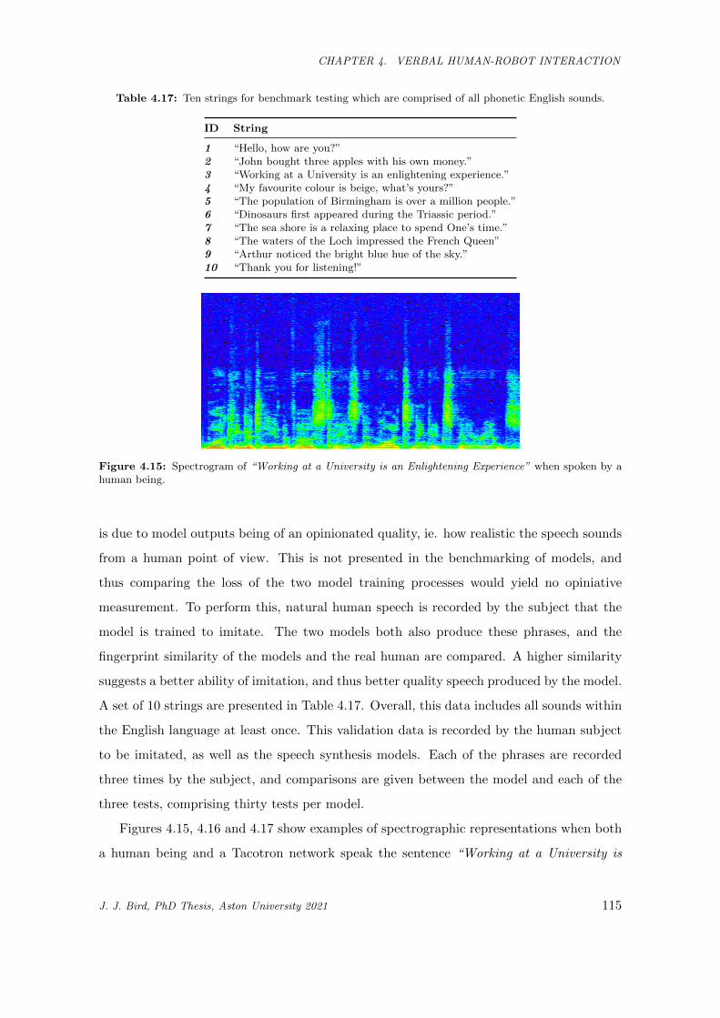
CHAPTER 4. VERBAL HUMAN-ROBOT INTERACTION
Table 4.17: Ten strings for benchmark testing which are comprised of all phonetic English sounds.
ID String
1 “Hello, how are you?”2 “John bought three apples with his own money.”3 “Working at a University is an enlightening experience.”4 “My favourite colour is beige, what’s yours?”5 “The population of Birmingham is over a million people.”6 “Dinosaurs first appeared during the Triassic period.”7 “The sea shore is a relaxing place to spend One’s time.”8 “The waters of the Loch impressed the French Queen”9 “Arthur noticed the bright blue hue of the sky.”10 “Thank you for listening!”
Figure 4.15: Spectrogram of “Working at a University is an Enlightening Experience” when spoken by ahuman being.
is due to model outputs being of an opinionated quality, ie. how realistic the speech sounds
from a human point of view. This is not presented in the benchmarking of models, and
thus comparing the loss of the two model training processes would yield no opiniative
measurement. To perform this, natural human speech is recorded by the subject that the
model is trained to imitate. The two models both also produce these phrases, and the
fingerprint similarity of the models and the real human are compared. A higher similarity
suggests a better ability of imitation, and thus better quality speech produced by the model.
A set of 10 strings are presented in Table 4.17. Overall, this data includes all sounds within
the English language at least once. This validation data is recorded by the human subject
to be imitated, as well as the speech synthesis models. Each of the phrases are recorded
three times by the subject, and comparisons are given between the model and each of the
three tests, comprising thirty tests per model.
Figures 4.15, 4.16 and 4.17 show examples of spectrographic representations when both
a human being and a Tacotron network speak the sentence “Working at a University is
J. J. Bird, PhD Thesis, Aston University 2021 115
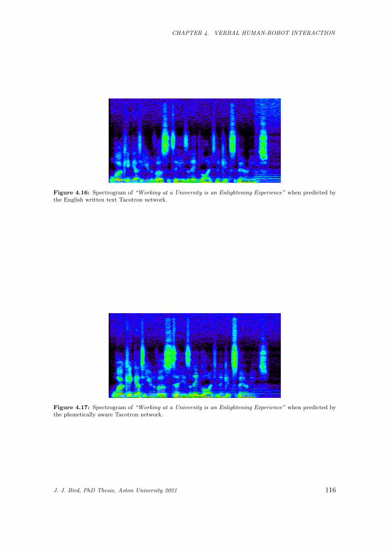
CHAPTER 4. VERBAL HUMAN-ROBOT INTERACTION
Figure 4.16: Spectrogram of “Working at a University is an Enlightening Experience” when predicted bythe English written text Tacotron network.
Figure 4.17: Spectrogram of “Working at a University is an Enlightening Experience” when predicted bythe phonetically aware Tacotron network.
J. J. Bird, PhD Thesis, Aston University 2021 116
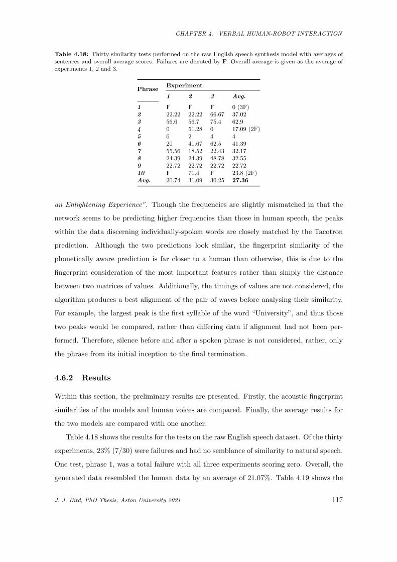
CHAPTER 4. VERBAL HUMAN-ROBOT INTERACTION
Table 4.18: Thirty similarity tests performed on the raw English speech synthesis model with averages ofsentences and overall average scores. Failures are denoted by F. Overall average is given as the average ofexperiments 1, 2 and 3.
PhraseExperiment
1 2 3 Avg.
1 F F F 0 (3F)2 22.22 22.22 66.67 37.023 56.6 56.7 75.4 62.94 0 51.28 0 17.09 (2F)5 6 2 4 46 20 41.67 62.5 41.397 55.56 18.52 22.43 32.178 24.39 24.39 48.78 32.559 22.72 22.72 22.72 22.7210 F 71.4 F 23.8 (2F)Avg. 20.74 31.09 30.25 27.36
an Enlightening Experience”. Though the frequencies are slightly mismatched in that the
network seems to be predicting higher frequencies than those in human speech, the peaks
within the data discerning individually-spoken words are closely matched by the Tacotron
prediction. Although the two predictions look similar, the fingerprint similarity of the
phonetically aware prediction is far closer to a human than otherwise, this is due to the
fingerprint consideration of the most important features rather than simply the distance
between two matrices of values. Additionally, the timings of values are not considered, the
algorithm produces a best alignment of the pair of waves before analysing their similarity.
For example, the largest peak is the first syllable of the word “University”, and thus those
two peaks would be compared, rather than differing data if alignment had not been per-
formed. Therefore, silence before and after a spoken phrase is not considered, rather, only
the phrase from its initial inception to the final termination.
4.6.2 Results
Within this section, the preliminary results are presented. Firstly, the acoustic fingerprint
similarities of the models and human voices are compared. Finally, the average results for
the two models are compared with one another.
Table 4.18 shows the results for the tests on the raw English speech dataset. Of the thirty
experiments, 23% (7/30) were failures and had no semblance of similarity to natural speech.
One test, phrase 1, was a total failure with all three experiments scoring zero. Overall, the
generated data resembled the human data by an average of 21.07%. Table 4.19 shows the
J. J. Bird, PhD Thesis, Aston University 2021 117
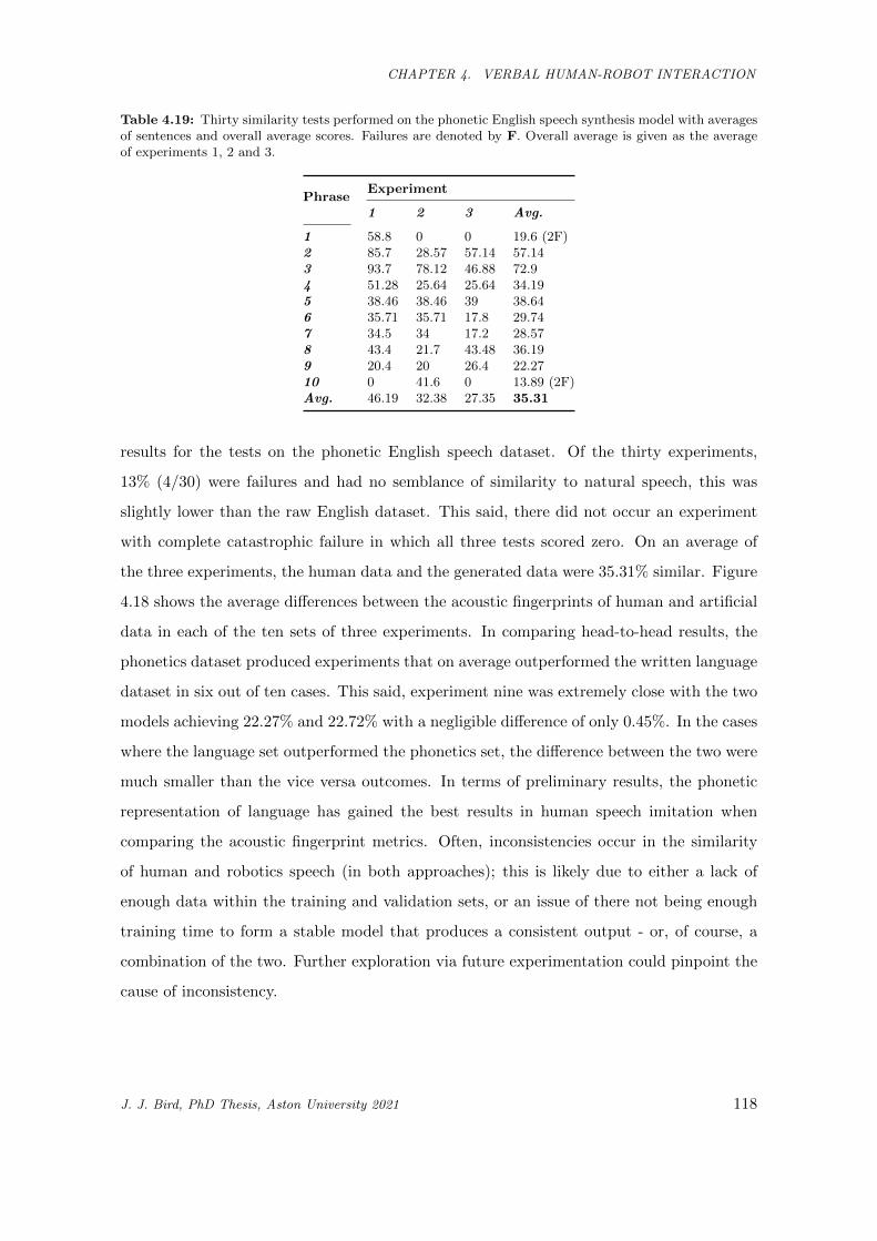
CHAPTER 4. VERBAL HUMAN-ROBOT INTERACTION
Table 4.19: Thirty similarity tests performed on the phonetic English speech synthesis model with averagesof sentences and overall average scores. Failures are denoted by F. Overall average is given as the averageof experiments 1, 2 and 3.
PhraseExperiment
1 2 3 Avg.
1 58.8 0 0 19.6 (2F)2 85.7 28.57 57.14 57.143 93.7 78.12 46.88 72.94 51.28 25.64 25.64 34.195 38.46 38.46 39 38.646 35.71 35.71 17.8 29.747 34.5 34 17.2 28.578 43.4 21.7 43.48 36.199 20.4 20 26.4 22.2710 0 41.6 0 13.89 (2F)Avg. 46.19 32.38 27.35 35.31
results for the tests on the phonetic English speech dataset. Of the thirty experiments,
13% (4/30) were failures and had no semblance of similarity to natural speech, this was
slightly lower than the raw English dataset. This said, there did not occur an experiment
with complete catastrophic failure in which all three tests scored zero. On an average of
the three experiments, the human data and the generated data were 35.31% similar. Figure
4.18 shows the average differences between the acoustic fingerprints of human and artificial
data in each of the ten sets of three experiments. In comparing head-to-head results, the
phonetics dataset produced experiments that on average outperformed the written language
dataset in six out of ten cases. This said, experiment nine was extremely close with the two
models achieving 22.27% and 22.72% with a negligible difference of only 0.45%. In the cases
where the language set outperformed the phonetics set, the difference between the two were
much smaller than the vice versa outcomes. In terms of preliminary results, the phonetic
representation of language has gained the best results in human speech imitation when
comparing the acoustic fingerprint metrics. Often, inconsistencies occur in the similarity
of human and robotics speech (in both approaches); this is likely due to either a lack of
enough data within the training and validation sets, or an issue of there not being enough
training time to form a stable model that produces a consistent output - or, of course, a
combination of the two. Further exploration via future experimentation could pinpoint the
cause of inconsistency.
J. J. Bird, PhD Thesis, Aston University 2021 118
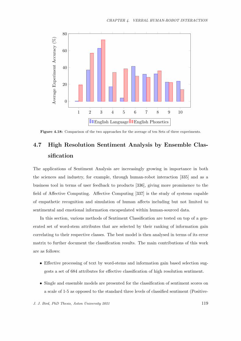
CHAPTER 4. VERBAL HUMAN-ROBOT INTERACTION
1 2 3 4 5 6 7 8 9 10
0
20
40
60
80
Average
Experim
entAccuracy
(%)
English Language English Phonetics
Figure 4.18: Comparison of the two approaches for the average of ten Sets of three experiments.
4.7 High Resolution Sentiment Analysis by Ensemble Clas-
sification
The applications of Sentiment Analysis are increasingly growing in importance in both
the sciences and industry, for example, through human-robot interaction [335] and as a
business tool in terms of user feedback to products [336], giving more prominence to the
field of Affective Computing. Affective Computing [337] is the study of systems capable
of empathetic recognition and simulation of human affects including but not limited to
sentimental and emotional information encapsulated within human-sourced data.
In this section, various methods of Sentiment Classification are tested on top of a gen-
erated set of word-stem attributes that are selected by their ranking of information gain
correlating to their respective classes. The best model is then analysed in terms of its error
matrix to further document the classification results. The main contributions of this work
are as follows:
• Effective processing of text by word-stems and information gain based selection sug-
gests a set of 684 attributes for effective classification of high resolution sentiment.
• Single and ensemble models are presented for the classification of sentiment scores on
a scale of 1-5 as opposed to the standard three levels of classified sentiment (Positive-
J. J. Bird, PhD Thesis, Aston University 2021 119
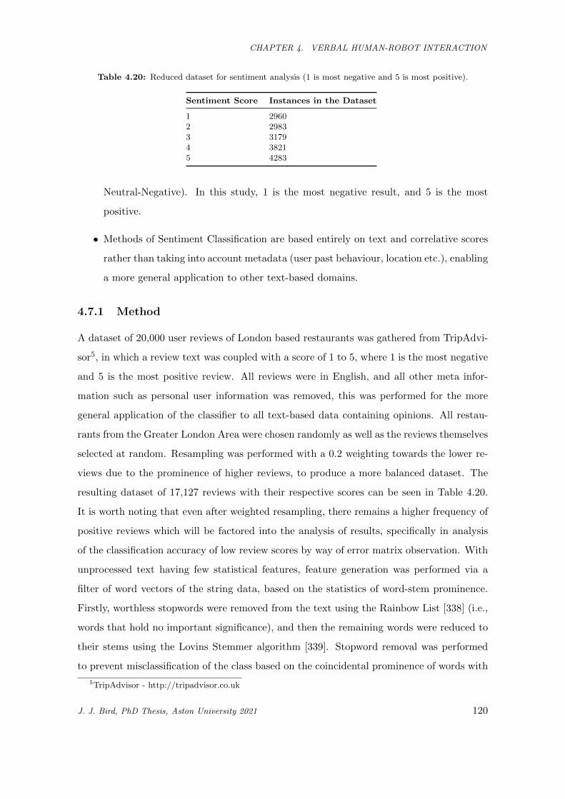
CHAPTER 4. VERBAL HUMAN-ROBOT INTERACTION
Table 4.20: Reduced dataset for sentiment analysis (1 is most negative and 5 is most positive).
Sentiment Score Instances in the Dataset
1 29602 29833 31794 38215 4283
Neutral-Negative). In this study, 1 is the most negative result, and 5 is the most
positive.
• Methods of Sentiment Classification are based entirely on text and correlative scores
rather than taking into account metadata (user past behaviour, location etc.), enabling
a more general application to other text-based domains.
4.7.1 Method
A dataset of 20,000 user reviews of London based restaurants was gathered from TripAdvi-
sor5, in which a review text was coupled with a score of 1 to 5, where 1 is the most negative
and 5 is the most positive review. All reviews were in English, and all other meta infor-
mation such as personal user information was removed, this was performed for the more
general application of the classifier to all text-based data containing opinions. All restau-
rants from the Greater London Area were chosen randomly as well as the reviews themselves
selected at random. Resampling was performed with a 0.2 weighting towards the lower re-
views due to the prominence of higher reviews, to produce a more balanced dataset. The
resulting dataset of 17,127 reviews with their respective scores can be seen in Table 4.20.
It is worth noting that even after weighted resampling, there remains a higher frequency of
positive reviews which will be factored into the analysis of results, specifically in analysis
of the classification accuracy of low review scores by way of error matrix observation. With
unprocessed text having few statistical features, feature generation was performed via a
filter of word vectors of the string data, based on the statistics of word-stem prominence.
Firstly, worthless stopwords were removed from the text using the Rainbow List [338] (i.e.,
words that hold no important significance), and then the remaining words were reduced to
their stems using the Lovins Stemmer algorithm [339]. Stopword removal was performed
to prevent misclassification of the class based on the coincidental prominence of words with
5TripAdvisor - http://tripadvisor.co.uk
J. J. Bird, PhD Thesis, Aston University 2021 120
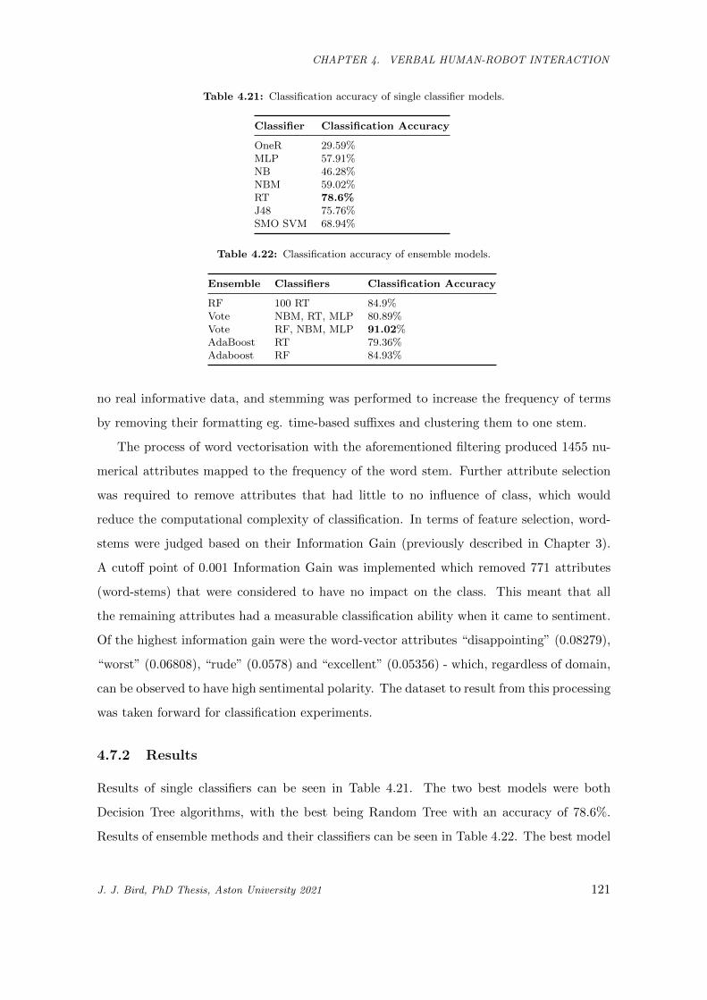
CHAPTER 4. VERBAL HUMAN-ROBOT INTERACTION
Table 4.21: Classification accuracy of single classifier models.
Classifier Classification Accuracy
OneR 29.59%MLP 57.91%NB 46.28%NBM 59.02%RT 78.6%J48 75.76%SMO SVM 68.94%
Table 4.22: Classification accuracy of ensemble models.
Ensemble Classifiers Classification Accuracy
RF 100 RT 84.9%Vote NBM, RT, MLP 80.89%Vote RF, NBM, MLP 91.02%AdaBoost RT 79.36%Adaboost RF 84.93%
no real informative data, and stemming was performed to increase the frequency of terms
by removing their formatting eg. time-based suffixes and clustering them to one stem.
The process of word vectorisation with the aforementioned filtering produced 1455 nu-
merical attributes mapped to the frequency of the word stem. Further attribute selection
was required to remove attributes that had little to no influence of class, which would
reduce the computational complexity of classification. In terms of feature selection, word-
stems were judged based on their Information Gain (previously described in Chapter 3).
A cutoff point of 0.001 Information Gain was implemented which removed 771 attributes
(word-stems) that were considered to have no impact on the class. This meant that all
the remaining attributes had a measurable classification ability when it came to sentiment.
Of the highest information gain were the word-vector attributes “disappointing” (0.08279),
“worst” (0.06808), “rude” (0.0578) and “excellent” (0.05356) - which, regardless of domain,
can be observed to have high sentimental polarity. The dataset to result from this processing
was taken forward for classification experiments.
4.7.2 Results
Results of single classifiers can be seen in Table 4.21. The two best models were both
Decision Tree algorithms, with the best being Random Tree with an accuracy of 78.6%.
Results of ensemble methods and their classifiers can be seen in Table 4.22. The best model
J. J. Bird, PhD Thesis, Aston University 2021 121
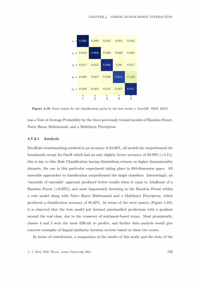
CHAPTER 4. VERBAL HUMAN-ROBOT INTERACTION
1 2 3 4 5
1
2
3
4
5
0.986 0.009 0.002 0.001 0.002
0.014 0.968 0.008 0.006 0.003
0.017 0.022 0.904 0.04 0.017
0.004 0.007 0.036 0.811 0.143
0.004 0.003 0.015 0.067 0.911
Figure 4.19: Error matrix for the classifications given by the best model, a Vote(RF, NBM, MLP)
was a Vote of Average Probability by the three previously trained models of Random Forest,
Naive Bayes Multinomial, and a Multilayer Perceptron.
4.7.2.1 Analysis
ZeroRules benchmarking resulted in an accuracy of 24.88%, all models far outperformed the
benchmark except for OneR which had an only slightly better accuracy of 29.59% (+4.71),
this is due to One Rule Classification having diminishing returns on higher dimensionality
datasets, the one in this particular experiment taking place in 684-dimension space. All
ensemble approaches to classification outperformed the single classifiers. Interestingly, an
‘ensemble of ensemble’ approach produced better results when it came to AdaBoost of a
Random Forest (+0.03%), and most importantly factoring in the Random Forest within
a vote model along with Naive Bayes Multinomial and a Multilayer Perceptron, which
produced a classification accuracy of 91.02%. In terms of the error matrix (Figure 4.19),
it is observed that the best model put forward misclassified predictions with a gradient
around the real class, due to the crossover of sentiment-based terms. Most prominently,
classes 4 and 5 were the most difficult to predict, and further data analysis would give
concrete examples of lingual similarity between reviews based on these two scores.
In terms of contribution, a comparison of the results of this study and the state of the
J. J. Bird, PhD Thesis, Aston University 2021 122
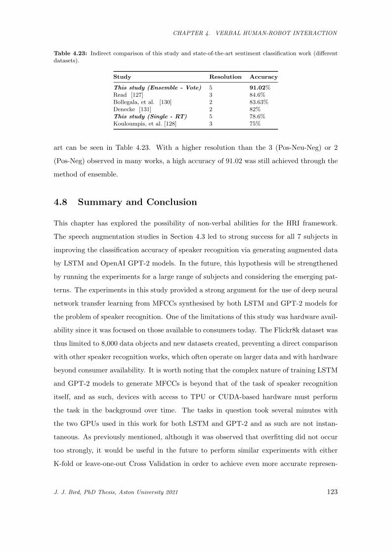
CHAPTER 4. VERBAL HUMAN-ROBOT INTERACTION
Table 4.23: Indirect comparison of this study and state-of-the-art sentiment classification work (differentdatasets).
Study Resolution Accuracy
This study (Ensemble - Vote) 5 91.02%Read [127] 3 84.6%Bollegala, et al. [130] 2 83.63%Denecke [131] 2 82%This study (Single - RT) 5 78.6%Kouloumpis, et al. [128] 3 75%
art can be seen in Table 4.23. With a higher resolution than the 3 (Pos-Neu-Neg) or 2
(Pos-Neg) observed in many works, a high accuracy of 91.02 was still achieved through the
method of ensemble.
4.8 Summary and Conclusion
This chapter has explored the possibility of non-verbal abilities for the HRI framework.
The speech augmentation studies in Section 4.3 led to strong success for all 7 subjects in
improving the classification accuracy of speaker recognition via generating augmented data
by LSTM and OpenAI GPT-2 models. In the future, this hypothesis will be strengthened
by running the experiments for a large range of subjects and considering the emerging pat-
terns. The experiments in this study provided a strong argument for the use of deep neural
network transfer learning from MFCCs synthesised by both LSTM and GPT-2 models for
the problem of speaker recognition. One of the limitations of this study was hardware avail-
ability since it was focused on those available to consumers today. The Flickr8k dataset was
thus limited to 8,000 data objects and new datasets created, preventing a direct comparison
with other speaker recognition works, which often operate on larger data and with hardware
beyond consumer availability. It is worth noting that the complex nature of training LSTM
and GPT-2 models to generate MFCCs is beyond that of the task of speaker recognition
itself, and as such, devices with access to TPU or CUDA-based hardware must perform
the task in the background over time. The tasks in question took several minutes with
the two GPUs used in this work for both LSTM and GPT-2 and as such are not instan-
taneous. As previously mentioned, although it was observed that overfitting did not occur
too strongly, it would be useful in the future to perform similar experiments with either
K-fold or leave-one-out Cross Validation in order to achieve even more accurate represen-
J. J. Bird, PhD Thesis, Aston University 2021 123
CHAPTER 4. VERBAL HUMAN-ROBOT INTERACTION
tations of the classification metrics. In terms of future applications, the then-optimised
model would be then implemented within real robots and smart home assistants through
compatible software. As found during the literature review, there has been a pattern of
GPT-2 being notably powerful in terms of dataset augmentation with a focus on written
language, given that GPT-2’s initial weights are trained via a large and complex text corpus
(Open WebText). Note that in Section 4.3, GPT-2 was often outperformed in some way
by the LSTM; it may be that these two points go hand in hand, and that GPT models
may provide a better solution in the future if and when trained on a comparatively large
dataset of natural speech in the form of MFCCs or other types of audio feature extraction
techniques.
To summarise Section 4.3, seven subjects were benchmarked with both a tuned LSTM
and OpenAI’s GPT-2 model. GPT-2 generated new data with hyperparameters tempera-
ture of 1, and selecting the topk of 1, in future other hyperparameters should be benchmarked
to better tune the GPT-2’s generative process for speech. Trials for model training were re-
peated multiple times with differing random seeds, but minuscule differences (< 10−4) were
noted in the metrics. Literature review saw that some research found promise in i-vector
representation [64, 65], if future exploration finds success in either temporal or attention-
based models to generate i-vectors then it would be promising for non-fixed length utterance
classification. Especially since it was found during data collection that the speed subjects
utter phrases differs greatly based on their accent. With larger scale testing based on the
knowledge from this part of the thesis, other speaker identification metrics[340] such as
Equal Error Rating based on a threshold of false accept rate equalling the false reject rate,
and various Detection Cost Functions etc. should be considered in order to further discern
the effects of introducing synthetic speech during model training. Additionally, in future,
as was seen with related works, a GAN could also be implemented to provide a third possi-
ble solution to the problem of data scarcity in speaker recognition as well as other related
speech recognition classification problems - bias is an open issue that has been noted for
data augmentation with GANs [341], and as such, this issue must be studied if a GAN
is implemented for problems of this nature. In terms of real world usage on devices, the
current computational costs of the models prior to further tuning and optimisation mean
that the training process could likely only be performed on newer models of Smartphones
with access to newer hardware. Execution and inference of the model incurs a relatively
J. J. Bird, PhD Thesis, Aston University 2021 124
CHAPTER 4. VERBAL HUMAN-ROBOT INTERACTION
lower computational cost, and so a larger range of devices could perform speaker recognition
if the model is trained via a cloud service or external machine and then deployed to the
device, additionally if execution is also performed on a cloud service then any device with
internet access could then run inference via the models presented in this work. One of the
main drawbacks of the suggested approach is the computational complexity of transformer
and temporal models, and as such smaller model architectures could be explored in the
future via either training from scratch or through similar to that performed by Michel et
al. [342]. It was demonstrated in Section 4.3 that data augmentation can aid in improving
speaker recognition for scarce datasets. Following the 14 successful runs including LSTMs
and GPT-2s, the overall process followed by the experiments could be scripted and thus
completely automated, allowing for the benchmarking of many more subjects to give a
much more generalised set of results, i.e., more representative of the general population.
Additionally, samples spoken from many languages could also be considered to provide lan-
guage generalisation, rather than just the English language spoken by multiple international
dialects in this study. Should generalisation be possible, future models may require only
a small amount of fine-tuning to produce synthetic speech for a given person rather than
training from scratch as was performed here. More generally, the transfer learning methods
presented here have the potential to improve additional areas of machine learning that have
not yet been attempted.
This study in Section 4.4 showed that hyper-heuristically optimising the topology of
an Artificial Neural Network led to a high classification ability of the MFCC data from
spoken phonetic sounds by both native and non-native English speakers. In addition to
this, in comparison to the Hidden Markov Model, models that required less computational
resources and yet still outperformed HMM were derived through a multi-objective algo-
rithm. Further work should explore a more fine-tuned minimisation of resources (λ2) since
a value of 0.9 seemed to be too extreme and produced weak results, and thus further pairs
weights should be explored towards this end. Following the success of both the single and
multi-objective approaches to hyperheuristic optimisation of phoneme classification, further
MLP parameters could be considered as those to be optimised, such as activation, training
time, momentum, and learning rate etc. In addition, further network architectures could be
considered for optimisation in order to explore the abilities and effects, such as temporally-
aware recurrence through RNN and Bi-directional LSTM which have shown promise in
J. J. Bird, PhD Thesis, Aston University 2021 125
CHAPTER 4. VERBAL HUMAN-ROBOT INTERACTION
recent advances in speech recognition [47, 257] and CNN with Bi-directional LSTM [343].
Improvements on these studies in the future could also consider the heuristic optimisation of
HMM hidden units, in a one-dimensional problem space, since the experiments in Section 4.4
focused on manual optimisation which was not exhaustive. Since the evolutionary method
was successful, in the future, other heuristic searches could be explored and compared, such
as Particle Swarm Optimisation or Ant Colony Optimisation, for example. Additionally,
the dataset could be expanded beyond the limited 6-subject data gathered to explore the
possibility of generalisation to a large dataset of phonetic utterances. In terms of the ideal
models produced, and with the post-construction of complete words, phrases, and sentences,
a speech recognition system could further be produced without the need for retraining in
future. That is, should English lexicon evolve, as it does often (in 2018, Merriam-Webster
added 800 new words to their dictionary [344]), speech recognition models would not re-
quire retraining; simply, these words would be constructed from already learnt phonetic
sounds. Thus, speech recognition systems would then only be hampered by the evolution
of phonetic structure in language; as was previously described, the evolution of phonetic
language occurs over great lengths of time, compared to which Machine Learning paradigms
become obsolete and replaced far quicker. To summarise Section 4.4, several evolutionar-
ily optimised Neural Network topologies of varying classification ability and computational
complexity were presented via both single and multi-objective approaches. The Hidden
Markov model was fine-tuned by a linear search, producing seven different models, all of
varying classification ability, with the strongest for classification being 150 hidden units.
All suggested ANN topologies outperformed the Hidden Markov Model in the phoneme
recognition problem within single-objective optimisation, whereas multi-objective optimi-
sation presented many solutions that required fewer resources to train, and in many cases,
lead to better classification ability. For real-time techniques such as lifelong learning of
an autonomous machine, some of the less complex multi-objective solutions are suggested
in situations such as the availability of only a single CPU, whereas, in a situation where
resources are not at a premium, single-objective solutions are suggested.
Following on from the findings in Section 4.4, Section 4.5 explored the effectiveness of
various machine learning techniques in terms of classifying the accent of the subject based
on recorded audio data. The diphthong phoneme sounds were succesfully classified into four
different accents from the UK and Mexico with an accuracy of 94.74% when a manually
J. J. Bird, PhD Thesis, Aston University 2021 126
CHAPTER 4. VERBAL HUMAN-ROBOT INTERACTION
tuned LSTM of 200 units and a Random Forest are ensembled through a vote of average
probability. Leave-one-out (LOO) cross-validation has been observed to be superior to test-
set and k-fold cross-validation techniques but requires far more processing time[224], this
study therefore would have been around 3000 times more complex due to there being 30,000
classifiable data objects. It is likely that more accurate results would be attained through
this approach but with the resources available, this was not possible. Furthermore, more
intense searching of the problem spaces of HMM and LSTM hidden unit selection should
be performed since relatively large differences were observed in minute topological changes.
Most importantly, a larger range of accent classes should be considered to more generalise
to populations.
The experiments in Section 4.6 then proposed the possibility of enriching speech data
with phonetic awareness to improve speech synthesis from a given text. Although re-
sults suggested the phoneme aware approaches were preliminarily more promising than raw
English notation, the phonetic awareness approach was faced with a disadvantage in the
fine-tuning process. The pre-existing model was trained on raw English language in a US
dialect and fine tuned for raw English language in British dialect as well as English pho-
netics in British dialect. Thus, the phonetic model would require more training in order
to overcome the disadvantaged starting point it faced. For a more succinct comparison,
future models should be trained from an initial random distribution of network weights
for their respective datasets. In addition to this, it must be pointed out that the input
data from the English written text dataset had 26 unique alphabetic values whereas this
is extended in the second dataset since there are 44 unique phonemes that make up the
spoken English language in a British dialect. Statistical validation through the comparison
of acoustic fingerprints are considered, with similarities to real speech compared to the same
input sentence or phrase. Though an acoustic fingerprint does give a concrete comparison
between pairs of output data, human opinion is still not properly reflected. For this, as
the Tacotron paper did, Mean Opinion Score (MOS) should also be performed. MOS is
given as MOS =∑N
n=1 Rn
N , where R are rating scores given by a subject group of N par-
ticipants. Thus, this is simply the average rating given by the audience. MOS requires a
large audience to give their opinions, denoted by a nominal score, to rate the networks in
terms of human hearing. Such MOS would allow for a second metric, real opinion, to also
provide a score. A multi-objective problem is then presented through the maximisation of
J. J. Bird, PhD Thesis, Aston University 2021 127
CHAPTER 4. VERBAL HUMAN-ROBOT INTERACTION
acoustic fingerprint similarities as well as the opinion of the audience. Additionally, other
spectrogram prediction paradigms such as Tacotron2 and DCTTS could be studied in terms
of the effects of English vs. Phonetic English. As mentioned in the previous subsection,
further work should also be performed for pinpointing the cause of inconsistent output from
the models. Explorations into the effects of there being a larger dataset as well as more
training time for the model could discover the cause of inconsistency and help to produce
a stronger training paradigm for speech synthesis.
To summarise Section 4.6, 100,000 extra iterations of training on top of a publicly
available dataset, then fine-tuned on a human dataset of only 1.6 hours worth of speech
translated to phonetic structure, produced a network with the ability to reproduce new
speech at 35.31% accuracy. It is not out of question whatsoever for postprocessing to
enable the data to be completely realistic, which could then be ‘leaked’ to the media, the
law, or otherwise. Such findings present a dangerous situation, in which a person’s speech
could be imitated to create the illusion of evidence that they have said such things that in
reality they have not. Although this section serves primarily as a method of maximising
artificial imitative abilities, it should also serve as a grave warning in order to minimise the
potential implications on an individual’s life. Future information security research should,
and arguably must, discover competing methods of detection of spoof speech in order to
prevent such cases. On the other hand, realistic speech synthesis could be used in real time
for more positive means, such as an augmented voice for those suffering illness that could
result in the loss of the ability of speech.
The experiments in Section 4.7 explored methods for high resolution sentiment analysis.
This section presented results from models for classification of multi-level sentiment at five
distinct levels after performing effective feature extraction based on lingual methods. The
best single classifier model was a Random Tree with a classification accuracy of 78.6%, which
was outperformed by all applied ensemble methods and their models. The best overall
model was an ensemble of Random Forest, Naive Bayes Multinomial, and a Multilayer
Perceptron through a Vote of Average Probability, with a classification accuracy of 91.02%.
These findings suggest future work is required in the development of text-based ensemble
classifiers as well as their single classification parameters, due to the trained models in
these experiments successfully being improved when part of an ensemble. The effectiveness
of Neural Networks for sentiment classification is well documented [345], implying that
J. J. Bird, PhD Thesis, Aston University 2021 128
CHAPTER 4. VERBAL HUMAN-ROBOT INTERACTION
further work with more computational resources than were available for these experiment
is needed due to the low results achieved. Successful experiments were performed purely
on a user’s message and no other meta-information (e.g., previous reviews, personal user
information) which not only shows effectiveness in the application in the original domain of
user review, but also a general application to other text-based domains such as chatbots and
keyword-based opinion mining. The applications of the classifiers put forward in Section 4.7
are useful in the aforementioned domains, although future work could encompass a larger
range of sources to smooth out some of the remaining domain-specific information.
To finally conclude this chapter, several experiments have led to multiple modules that
are to be unified in the final framework. This chapter explored several technologies that
were verbal in nature, which included recognition of the speaker and how synthetic data
can improve this process, phoneme recognition in audio (by ability and resource usage) for
both phoneme and accent classification of speakers, synthesis of speech and how phonetic
representation seemingly improved speech synthesis in preliminary tests with an example
of the audio files produced by the two models, and finally a multi-level sentiment analysis
model that considered extra sentiments outside of the classical neg-neu-pos approaches. The
studies therefore complement one another and lead to the verbal abilities of the HRI frame-
work; accents can be recognised, phonemes can be classified from speech, and also, data
augmentation can be performed to autonomously improve the recognition of the speaker
from their voice. Following all of this, sentiment analysis can then be performed on the
recognised speech. Given these abilities, the HRI framework can then interact with human
beings via spoken communication, which then leads to further interaction and task delib-
eration. Towards the end of this thesis, in Chapter 7, further integration can be observed
based on the findings in this Chapter, where commands are further deliberated upon and
tasks are performed.
The ability to understand speech aids the robot during the input stage. Audio can
be considered, and a textual representation of utterances can be generated. Following
this operation, the framework will now have text as input, which can be considered by
the subsequent modules and deliberated upon. With the particular implementation of
phoneme-aware speech recognition, as the experiments in this chapter found to be possible,
this may lead to a speech recognition module which would not need to be retrained when
new words or phrases are added. Since all words are constructed from a set of phonemes, a
J. J. Bird, PhD Thesis, Aston University 2021 129

CHAPTER 4. VERBAL HUMAN-ROBOT INTERACTION
dictionary is required in place of spending computational resources to retrain the module.
The classification of sentiment also provides useful information as input to the framework,
since both text and sentiment could, in some cases, better describe the inputs. Towards the
interpersonal abilities of the HRI framework, the recognition of speakers would allow for
outputs to be engineered and personalised specifically to an individual. In another case of
interpersonal ability but regarding output, being able to respond in a realistic human voice
aids in improving the HRI experience.
J. J. Bird, PhD Thesis, Aston University 2021 130
CHAPTER 5. NON-VERBAL INTERACTION
Chapter 5
Non-Verbal Human-Robot
Interaction
5.1 Introduction
Non-verbal interaction is the ability to convey social interaction without the voice (or in
addition to the voice). For example, if a person asks another a question, and they respond
with a thumbs up, this non-verbal interaction can be inferred as an affirmative answer or a
positive sentiment depending on what the question was. In this interaction, the thumbs up
gesture has been ’classified’ by the other person via their vision, but the activity that led to
this gesture was nervous and then electromyographic in nature and could thus be recognised
by these activities. To give another example, the answer to ”are you concentrating?” (in the
casual sense) could be responded to and inferred with speech. This could also be interpreted
by the electrical activities within the lobe and classified in this way, effectively removing
the need for the subject to have to convey their state. These examples given are from some
of the experiments explored in this chapter.
Similarly to the previous chapter, this chapter presents several experiments for non-
verbal communication with machines which have individual scientific contributions pre-
sented where appropriate within the section introductions. Given the nature of the ex-
periments sharing a background of biological signal processing, an overall background sec-
tion is given initially. This section explores classification of electroencephalographic and
electromyographic signals as well as transfer learning between them by models since bio-
J. J. Bird, PhD Thesis, Aston University 2021 131
CHAPTER 5. NON-VERBAL INTERACTION
electrical natures are shared to an extent. In addition, the classification of signals is also
notably improved when the training data is augmented with synthetic signals produced by
transformer-based models (similarly to the speaker recognition experiments in the previous
chapter).
5.2 Biosignal Processing
5.2.1 Electroencephalography
Brain-Computer Interfaces (BCI) are devices that allow for direct communication between
the brain and a computer [346]. By skipping the usual brain outputs of nerves and mus-
cles, BCIs allow for the interpretation of brain activity directly as a form of control. For
example, enabling a cursor on a screen to be moved by thought alone [347], rather than
through muscular movements of the arm and hand to interact with a physical mouse. The
majority of BCIs record and process eelctroencephalographic data from the brain. Elec-
troencephalography (EEG) is the measurement and recording of electrical activity produced
by the brain [348]. The collection of EEG data is carried out through the use of applied
electrodes, which reads the minute electrophysiological currents produced by the brain due
to nervous oscillation [349, 350]. The most invasive form of EEG is subdural [351] in
which electrodes are placed directly on the brain itself. Far less invasive techniques require
electrodes to be placed around the cranium, of which the disadvantage is that signals are
being read through the thick bone of the skull [352]. Raw electrical data is measured in
microvolts (uV ), which over time produce wave patterns. Several electroencephalographic
methods compose the state-of-the-art in the field. These include the P300 [353] which is a
wave thought to be involved in decision making, elicited by interrupting a repeated stimulus
with an infrequent event - P300 has been used to allow for brain-machine control of digital
text [354]. Similarly, Contingent Negative Variation (CNV) [355], an event-related potential
component related to the reaction between warning and action signals, has been shown to
predict potential movement intention [356].
Machine learning techniques with inputs being that of statistical features of the wave
are commonly used to classify mental states [133, 132] for brain-machine interaction, where
states are used as dimensions of user input. Probabilistic methods such as Deep Belief Net-
works, Support Vector Machines, and various types of neural networks have been found to
J. J. Bird, PhD Thesis, Aston University 2021 132
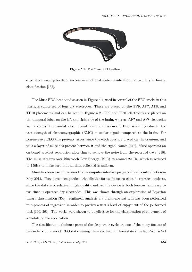
CHAPTER 5. NON-VERBAL INTERACTION
Figure 5.1: The Muse EEG headband.
experience varying levels of success in emotional state classification, particularly in binary
classification [135].
The Muse EEG headband as seen in Figure 5.1, used in several of the EEG works in this
thesis, is comprised of four dry electrodes. These are placed on the TP9, AF7, AF8, and
TP10 placements and can be seen in Figure 5.2. TP9 and TP10 electrodes are placed on
the temporal lobes on the left and right side of the brain, whereas AF7 and AF8 electrodes
are placed on the frontal lobe. Signal noise often occurs in EEG recordings due to the
vast strength of electromyographic (EMG) muscular signals compared to the brain. For
non-invasive EEG this presents issues, since the electrodes are placed on the cranium, and
thus a layer of muscle is present between it and the signal source [357]. Muse operates an
on-board artefact separation algorithm to remove the noise from the recorded data [358].
The muse streams over Bluetooth Low Energy (BLE) at around 220Hz, which is reduced
to 150Hz to make sure that all data collected is uniform.
Muse has been used in various Brain-computer interface projects since its introduction in
May 2014. They have been particularly effective for use in neuroscientific research projects,
since the data is of relatively high quality and yet the device is both low-cost and easy to
use since it operates dry electrodes. This was shown through an exploration of Bayesian
binary classification [359]. Sentiment analysis via brainwave patterns has been performed
in a process of regression in order to predict a user’s level of enjoyment of the performed
task [360, 361]. The works were shown to be effective for the classification of enjoyment of
a mobile phone application.
The classification of minute parts of the sleep-wake cycle are one of the many focuses of
researchers in terms of EEG data mining. Low resolution, three-state (awake, sleep, REM
J. J. Bird, PhD Thesis, Aston University 2021 133
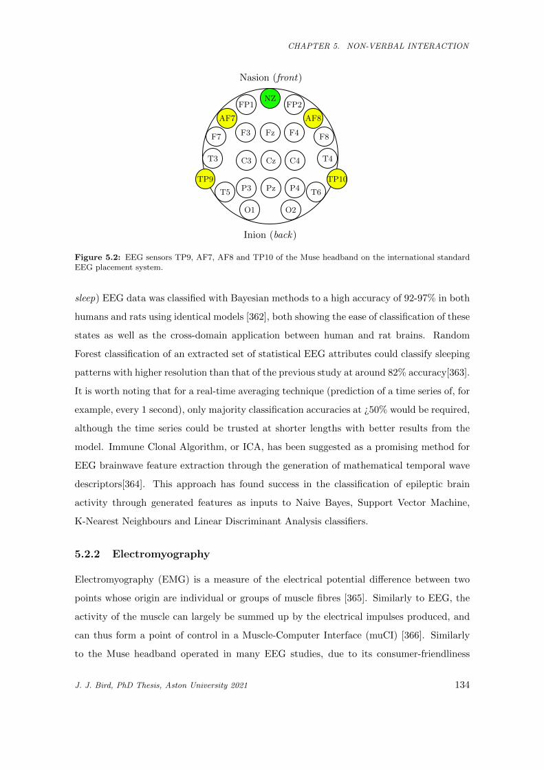
CHAPTER 5. NON-VERBAL INTERACTION
Nasion (front)
Inion (back)
NZFP1 FP2
AF7 AF8
TP9 TP10
F7 F8FzF3 F4
CzC3 C4T3 T4
PzP3 P4T5 T6
O1 O2
Figure 5.2: EEG sensors TP9, AF7, AF8 and TP10 of the Muse headband on the international standardEEG placement system.
sleep) EEG data was classified with Bayesian methods to a high accuracy of 92-97% in both
humans and rats using identical models [362], both showing the ease of classification of these
states as well as the cross-domain application between human and rat brains. Random
Forest classification of an extracted set of statistical EEG attributes could classify sleeping
patterns with higher resolution than that of the previous study at around 82% accuracy[363].
It is worth noting that for a real-time averaging technique (prediction of a time series of, for
example, every 1 second), only majority classification accuracies at ¿50% would be required,
although the time series could be trusted at shorter lengths with better results from the
model. Immune Clonal Algorithm, or ICA, has been suggested as a promising method for
EEG brainwave feature extraction through the generation of mathematical temporal wave
descriptors[364]. This approach has found success in the classification of epileptic brain
activity through generated features as inputs to Naive Bayes, Support Vector Machine,
K-Nearest Neighbours and Linear Discriminant Analysis classifiers.
5.2.2 Electromyography
Electromyography (EMG) is a measure of the electrical potential difference between two
points whose origin are individual or groups of muscle fibres [365]. Similarly to EEG, the
activity of the muscle can largely be summed up by the electrical impulses produced, and
can thus form a point of control in a Muscle-Computer Interface (muCI) [366]. Similarly
to the Muse headband operated in many EEG studies, due to its consumer-friendliness
J. J. Bird, PhD Thesis, Aston University 2021 134
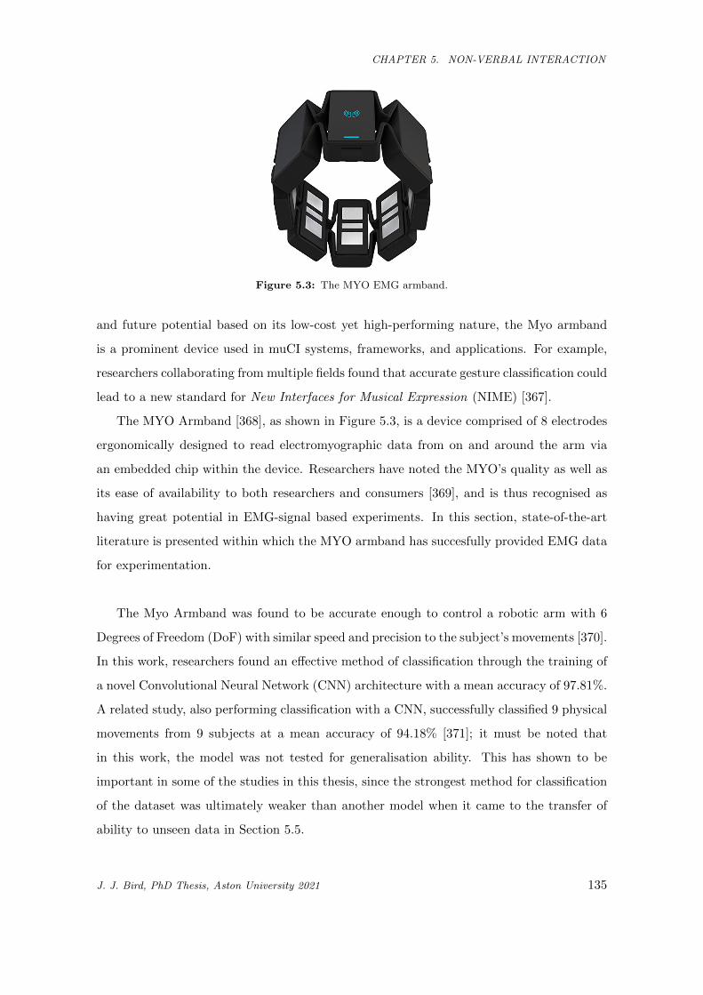
CHAPTER 5. NON-VERBAL INTERACTION
Figure 5.3: The MYO EMG armband.
and future potential based on its low-cost yet high-performing nature, the Myo armband
is a prominent device used in muCI systems, frameworks, and applications. For example,
researchers collaborating from multiple fields found that accurate gesture classification could
lead to a new standard for New Interfaces for Musical Expression (NIME) [367].
The MYO Armband [368], as shown in Figure 5.3, is a device comprised of 8 electrodes
ergonomically designed to read electromyographic data from on and around the arm via
an embedded chip within the device. Researchers have noted the MYO’s quality as well as
its ease of availability to both researchers and consumers [369], and is thus recognised as
having great potential in EMG-signal based experiments. In this section, state-of-the-art
literature is presented within which the MYO armband has succesfully provided EMG data
for experimentation.
The Myo Armband was found to be accurate enough to control a robotic arm with 6
Degrees of Freedom (DoF) with similar speed and precision to the subject’s movements [370].
In this work, researchers found an effective method of classification through the training of
a novel Convolutional Neural Network (CNN) architecture with a mean accuracy of 97.81%.
A related study, also performing classification with a CNN, successfully classified 9 physical
movements from 9 subjects at a mean accuracy of 94.18% [371]; it must be noted that
in this work, the model was not tested for generalisation ability. This has shown to be
important in some of the studies in this thesis, since the strongest method for classification
of the dataset was ultimately weaker than another model when it came to the transfer of
ability to unseen data in Section 5.5.
J. J. Bird, PhD Thesis, Aston University 2021 135
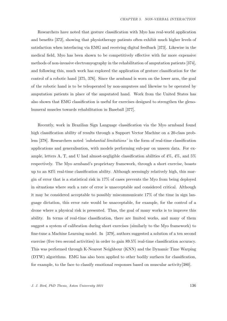
CHAPTER 5. NON-VERBAL INTERACTION
Researchers have noted that gesture classification with Myo has real-world application
and benefits [372], showing that physiotherapy patients often exhibit much higher levels of
satisfaction when interfacing via EMG and receiving digital feedback [373]. Likewise in the
medical field, Myo has been shown to be competitively effective with far more expensive
methods of non-invasive electromyography in the rehabilitation of amputation patients [374],
and following this, much work has explored the application of gesture classification for the
control of a robotic hand [375, 376]. Since the armband is worn on the lower arm, the goal
of the robotic hand is to be teleoperated by non-amputees and likewise to be operated by
amputation patients in place of the amputated hand. Work from the United States has
also shown that EMG classification is useful for exercises designed to strengthen the gleno-
humeral muscles towards rehabilitation in Baseball [377].
Recently, work in Brazilian Sign Language classification via the Myo armband found
high classification ability of results through a Support Vector Machine on a 20-class prob-
lem [378]. Researchers noted ’substantial limitations’ in the form of real-time classification
applications and generalisation, with models performing sub-par on unseen data. For ex-
ample, letters A, T, and U had almost-negligible classification abilities of 4%, 4%, and 5%
respectively. The Myo armband’s proprietary framework, through a short exercise, boasts
up to an 83% real-time classification ability. Although seemingly relatively high, this mar-
gin of error that is a statistical risk in 17% of cases prevents the Myo from being deployed
in situations where such a rate of error is unacceptable and considered critical. Although
it may be considered acceptable to possibly miscommunicate 17% of the time in sign lan-
guage dictation, this error rate would be unacceptable, for example, for the control of a
drone where a physical risk is presented. Thus, the goal of many works is to improve this
ability. In terms of real-time classification, there are limited works, and many of them
suggest a system of calibration during short exercises (similarly to the Myo framework) to
fine-tune a Machine Learning model. In [379], authors suggested a solution of a ten second
exercise (five two second activities) in order to gain 89.5% real-time classification accuracy.
This was performed through K-Nearest Neighbour (KNN) and the Dynamic Time Warping
(DTW) algorithms. EMG has also been applied to other bodily surfaces for classification,
for example, to the face to classify emotional responses based on muscular activity[380].
J. J. Bird, PhD Thesis, Aston University 2021 136
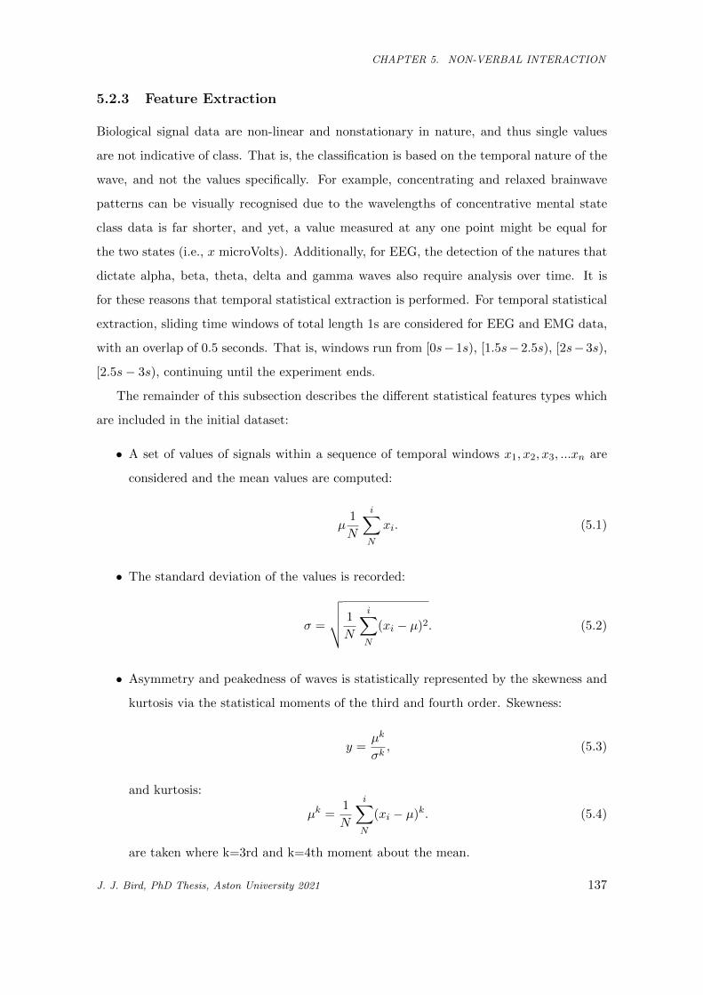
CHAPTER 5. NON-VERBAL INTERACTION
5.2.3 Feature Extraction
Biological signal data are non-linear and nonstationary in nature, and thus single values
are not indicative of class. That is, the classification is based on the temporal nature of the
wave, and not the values specifically. For example, concentrating and relaxed brainwave
patterns can be visually recognised due to the wavelengths of concentrative mental state
class data is far shorter, and yet, a value measured at any one point might be equal for
the two states (i.e., x microVolts). Additionally, for EEG, the detection of the natures that
dictate alpha, beta, theta, delta and gamma waves also require analysis over time. It is
for these reasons that temporal statistical extraction is performed. For temporal statistical
extraction, sliding time windows of total length 1s are considered for EEG and EMG data,
with an overlap of 0.5 seconds. That is, windows run from [0s− 1s), [1.5s− 2.5s), [2s− 3s),
[2.5s− 3s), continuing until the experiment ends.
The remainder of this subsection describes the different statistical features types which
are included in the initial dataset:
• A set of values of signals within a sequence of temporal windows x1, x2, x3, ...xn are
considered and the mean values are computed:
µ1
N
i∑N
xi. (5.1)
• The standard deviation of the values is recorded:
σ =
⌜⎷ 1
N
i∑N
(xi − µ)2. (5.2)
• Asymmetry and peakedness of waves is statistically represented by the skewness and
kurtosis via the statistical moments of the third and fourth order. Skewness:
y =µk
σk, (5.3)
and kurtosis:
µk =1
N
i∑N
(xi − µ)k. (5.4)
are taken where k=3rd and k=4th moment about the mean.
J. J. Bird, PhD Thesis, Aston University 2021 137
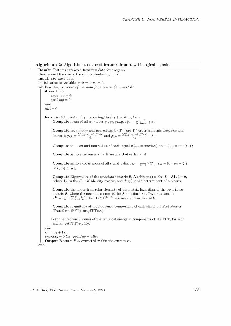
CHAPTER 5. NON-VERBAL INTERACTION
Algorithm 2: Algorithm to extract features from raw biological signals.Result: Features extracted from raw data for every wt
User defined the size of the sliding window wt = 1s;Input: raw wave data;Initialisation of variables init = 1, wt = 0;while getting sequence of raw data from sensor (> 1min) do
if init thenprev lag = 0;post lag = 1;
endinit = 0;;for each slide window (wt − prev lag) to (wt + post lag) do
Compute mean of all wt values y1, y2, y3...yn; yk = 1N
∑Ni=1 yki ;
;
Compute asymmetry and peakedness by 3rd and 4th order moments skewness and
kurtosis g1,k =∑N
i=1(yki−yk)3/N
s3k
and g2,k =∑N
i=1(yki−yk)4/N
s4k
− 3 ;
;Compute the max and min values of each signal wt
max = max(wt) and wtmin = min(wt) ;
;Compute sample variances K ×K matrix S of each signal
;
Compute sample covariances of all signal pairs, skℓ = 1N−1
∑Ni=1 (yki − yk) (yℓi − yℓ) ;
∀ k, ℓ ∈ [1,K];;Compute Eigenvalues of the covariance matrix S, λ solutions to: det (S− λIK) = 0,where IK is the K ×K identity matrix, and det(·) is the determinant of a matrix;
;Compute the upper triangular elements of the matrix logarithm of the covariancematrix S, where the matrix exponential for S is defined via Taylor expansioneB = IK +
∑∞n=1
Sn
n!, then B ∈ CK×K is a matrix logarithm of S;
;Compute magnitude of the frequency components of each signal via Fast FourierTransform (FFT), magFFT(wt);
;Get the frequency values of the ten most energetic components of the FFT, for each
signal, getFFT(wt, 10);
endwt = wt + 1s;prev lag = 0.5s; post lag = 1.5s;Output Features Fwt extracted within the current wt
end
J. J. Bird, PhD Thesis, Aston University 2021 138
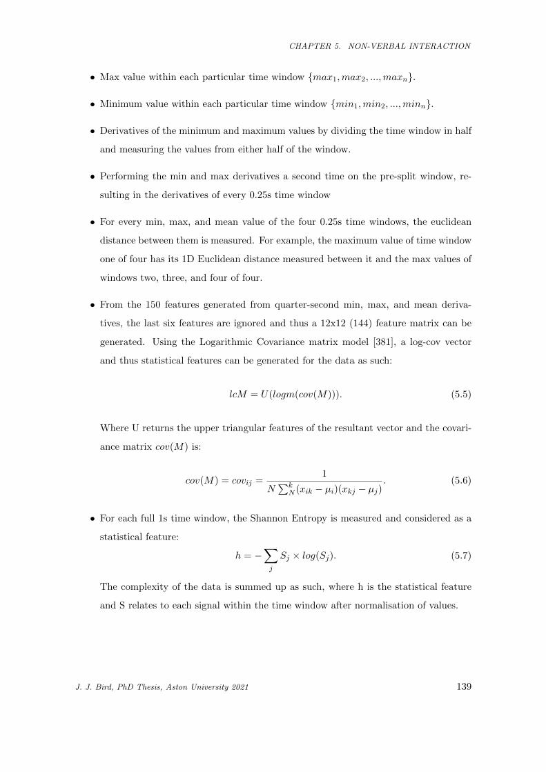
CHAPTER 5. NON-VERBAL INTERACTION
• Max value within each particular time window {max1,max2, ...,maxn}.
• Minimum value within each particular time window {min1,min2, ...,minn}.
• Derivatives of the minimum and maximum values by dividing the time window in half
and measuring the values from either half of the window.
• Performing the min and max derivatives a second time on the pre-split window, re-
sulting in the derivatives of every 0.25s time window
• For every min, max, and mean value of the four 0.25s time windows, the euclidean
distance between them is measured. For example, the maximum value of time window
one of four has its 1D Euclidean distance measured between it and the max values of
windows two, three, and four of four.
• From the 150 features generated from quarter-second min, max, and mean deriva-
tives, the last six features are ignored and thus a 12x12 (144) feature matrix can be
generated. Using the Logarithmic Covariance matrix model [381], a log-cov vector
and thus statistical features can be generated for the data as such:
lcM = U(logm(cov(M))). (5.5)
Where U returns the upper triangular features of the resultant vector and the covari-
ance matrix cov(M) is:
cov(M) = covij =1
N∑k
N (xik − µi)(xkj − µj). (5.6)
• For each full 1s time window, the Shannon Entropy is measured and considered as a
statistical feature:
h = −∑j
Sj × log(Sj). (5.7)
The complexity of the data is summed up as such, where h is the statistical feature
and S relates to each signal within the time window after normalisation of values.
J. J. Bird, PhD Thesis, Aston University 2021 139
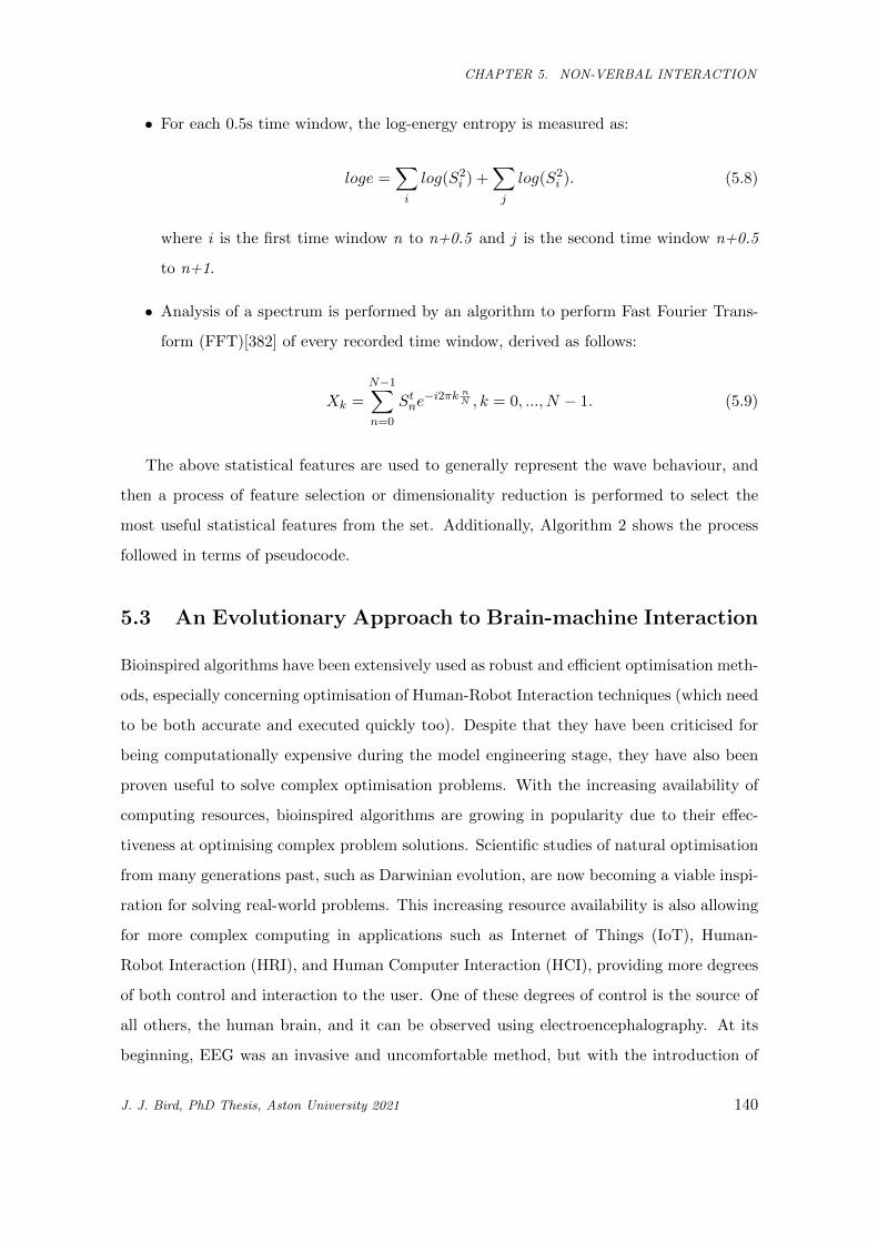
CHAPTER 5. NON-VERBAL INTERACTION
• For each 0.5s time window, the log-energy entropy is measured as:
loge =∑i
log(S2i ) +
∑j
log(S2i ). (5.8)
where i is the first time window n to n+0.5 and j is the second time window n+0.5
to n+1.
• Analysis of a spectrum is performed by an algorithm to perform Fast Fourier Trans-
form (FFT)[382] of every recorded time window, derived as follows:
Xk =
N−1∑n=0
Stne
−i2πk nN , k = 0, ..., N − 1. (5.9)
The above statistical features are used to generally represent the wave behaviour, and
then a process of feature selection or dimensionality reduction is performed to select the
most useful statistical features from the set. Additionally, Algorithm 2 shows the process
followed in terms of pseudocode.
5.3 An Evolutionary Approach to Brain-machine Interaction
Bioinspired algorithms have been extensively used as robust and efficient optimisation meth-
ods, especially concerning optimisation of Human-Robot Interaction techniques (which need
to be both accurate and executed quickly too). Despite that they have been criticised for
being computationally expensive during the model engineering stage, they have also been
proven useful to solve complex optimisation problems. With the increasing availability of
computing resources, bioinspired algorithms are growing in popularity due to their effec-
tiveness at optimising complex problem solutions. Scientific studies of natural optimisation
from many generations past, such as Darwinian evolution, are now becoming a viable inspi-
ration for solving real-world problems. This increasing resource availability is also allowing
for more complex computing in applications such as Internet of Things (IoT), Human-
Robot Interaction (HRI), and Human Computer Interaction (HCI), providing more degrees
of both control and interaction to the user. One of these degrees of control is the source of
all others, the human brain, and it can be observed using electroencephalography. At its
beginning, EEG was an invasive and uncomfortable method, but with the introduction of
J. J. Bird, PhD Thesis, Aston University 2021 140
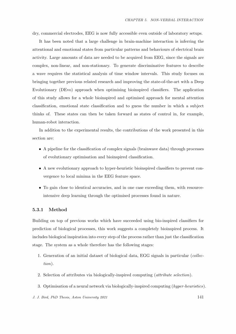
CHAPTER 5. NON-VERBAL INTERACTION
dry, commercial electrodes, EEG is now fully accessible even outside of laboratory setups.
It has been noted that a large challenge in brain-machine interaction is inferring the
attentional and emotional states from particular patterns and behaviours of electrical brain
activity. Large amounts of data are needed to be acquired from EEG, since the signals are
complex, non-linear, and non-stationary. To generate discriminative features to describe
a wave requires the statistical analysis of time window intervals. This study focuses on
bringing together previous related research and improving the state-of-the-art with a Deep
Evolutionary (DEvo) approach when optimising bioinspired classifiers. The application
of this study allows for a whole bioinspired and optimised approach for mental attention
classification, emotional state classification and to guess the number in which a subject
thinks of. These states can then be taken forward as states of control in, for example,
human-robot interaction.
In addition to the experimental results, the contributions of the work presented in this
section are:
• A pipeline for the classification of complex signals (brainwave data) through processes
of evolutionary optimisation and bioinspired classification.
• A new evolutionary approach to hyper-heuristic bioinspired classifiers to prevent con-
vergence to local minima in the EEG feature space.
• To gain close to identical accuracies, and in one case exceeding them, with resource-
intensive deep learning through the optimised processes found in nature.
5.3.1 Method
Building on top of previous works which have succeeded using bio-inspired classifiers for
prediction of biological processes, this work suggests a completely bioinspired process. It
includes biological inspiration into every step of the process rather than just the classification
stage. The system as a whole therefore has the following stages:
1. Generation of an initial dataset of biological data, EGG signals in particular (collec-
tion).
2. Selection of attributes via biologically-inspired computing (attribute selection).
3. Optimisation of a neural network via biologically-inspired computing (hyper-heuristics).
J. J. Bird, PhD Thesis, Aston University 2021 141
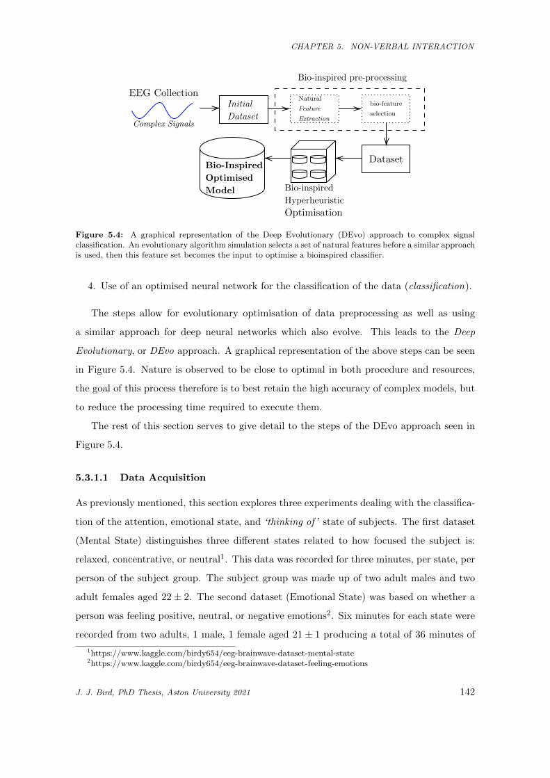
CHAPTER 5. NON-VERBAL INTERACTION
EEG CollectionInitial
Dataset
Natural
Feature
Extraction
Bio-Inspired
Optimised
Model
bio-feature
selection
Bio-inspired pre-processing
Dataset
Bio-inspired
Hyperheuristic
Optimisation
Complex Signals
Figure 5.4: A graphical representation of the Deep Evolutionary (DEvo) approach to complex signalclassification. An evolutionary algorithm simulation selects a set of natural features before a similar approachis used, then this feature set becomes the input to optimise a bioinspired classifier.
4. Use of an optimised neural network for the classification of the data (classification).
The steps allow for evolutionary optimisation of data preprocessing as well as using
a similar approach for deep neural networks which also evolve. This leads to the Deep
Evolutionary, or DEvo approach. A graphical representation of the above steps can be seen
in Figure 5.4. Nature is observed to be close to optimal in both procedure and resources,
the goal of this process therefore is to best retain the high accuracy of complex models, but
to reduce the processing time required to execute them.
The rest of this section serves to give detail to the steps of the DEvo approach seen in
Figure 5.4.
5.3.1.1 Data Acquisition
As previously mentioned, this section explores three experiments dealing with the classifica-
tion of the attention, emotional state, and ‘thinking of’ state of subjects. The first dataset
(Mental State) distinguishes three different states related to how focused the subject is:
relaxed, concentrative, or neutral1. This data was recorded for three minutes, per state, per
person of the subject group. The subject group was made up of two adult males and two
adult females aged 22± 2. The second dataset (Emotional State) was based on whether a
person was feeling positive, neutral, or negative emotions2. Six minutes for each state were
recorded from two adults, 1 male, 1 female aged 21± 1 producing a total of 36 minutes of
1https://www.kaggle.com/birdy654/eeg-brainwave-dataset-mental-state2https://www.kaggle.com/birdy654/eeg-brainwave-dataset-feeling-emotions
J. J. Bird, PhD Thesis, Aston University 2021 142
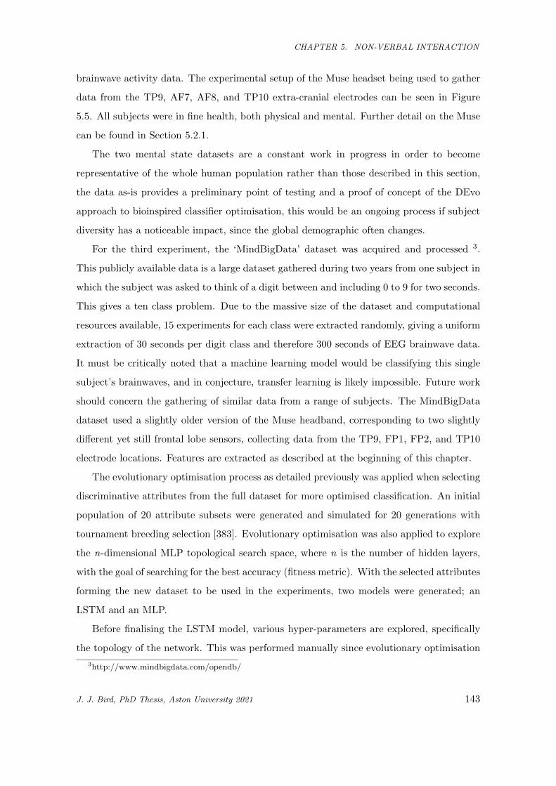
CHAPTER 5. NON-VERBAL INTERACTION
brainwave activity data. The experimental setup of the Muse headset being used to gather
data from the TP9, AF7, AF8, and TP10 extra-cranial electrodes can be seen in Figure
5.5. All subjects were in fine health, both physical and mental. Further detail on the Muse
can be found in Section 5.2.1.
The two mental state datasets are a constant work in progress in order to become
representative of the whole human population rather than those described in this section,
the data as-is provides a preliminary point of testing and a proof of concept of the DEvo
approach to bioinspired classifier optimisation, this would be an ongoing process if subject
diversity has a noticeable impact, since the global demographic often changes.
For the third experiment, the ‘MindBigData’ dataset was acquired and processed 3.
This publicly available data is a large dataset gathered during two years from one subject in
which the subject was asked to think of a digit between and including 0 to 9 for two seconds.
This gives a ten class problem. Due to the massive size of the dataset and computational
resources available, 15 experiments for each class were extracted randomly, giving a uniform
extraction of 30 seconds per digit class and therefore 300 seconds of EEG brainwave data.
It must be critically noted that a machine learning model would be classifying this single
subject’s brainwaves, and in conjecture, transfer learning is likely impossible. Future work
should concern the gathering of similar data from a range of subjects. The MindBigData
dataset used a slightly older version of the Muse headband, corresponding to two slightly
different yet still frontal lobe sensors, collecting data from the TP9, FP1, FP2, and TP10
electrode locations. Features are extracted as described at the beginning of this chapter.
The evolutionary optimisation process as detailed previously was applied when selecting
discriminative attributes from the full dataset for more optimised classification. An initial
population of 20 attribute subsets were generated and simulated for 20 generations with
tournament breeding selection [383]. Evolutionary optimisation was also applied to explore
the n-dimensional MLP topological search space, where n is the number of hidden layers,
with the goal of searching for the best accuracy (fitness metric). With the selected attributes
forming the new dataset to be used in the experiments, two models were generated; an
LSTM and an MLP.
Before finalising the LSTM model, various hyper-parameters are explored, specifically
the topology of the network. This was performed manually since evolutionary optimisation
3http://www.mindbigdata.com/opendb/
J. J. Bird, PhD Thesis, Aston University 2021 143
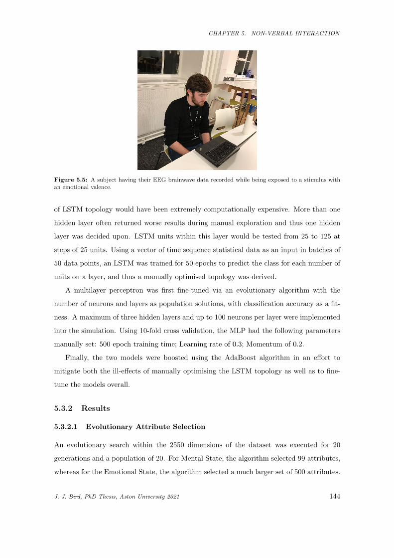
CHAPTER 5. NON-VERBAL INTERACTION
Figure 5.5: A subject having their EEG brainwave data recorded while being exposed to a stimulus withan emotional valence.
of LSTM topology would have been extremely computationally expensive. More than one
hidden layer often returned worse results during manual exploration and thus one hidden
layer was decided upon. LSTM units within this layer would be tested from 25 to 125 at
steps of 25 units. Using a vector of time sequence statistical data as an input in batches of
50 data points, an LSTM was trained for 50 epochs to predict the class for each number of
units on a layer, and thus a manually optimised topology was derived.
A multilayer perceptron was first fine-tuned via an evolutionary algorithm with the
number of neurons and layers as population solutions, with classification accuracy as a fit-
ness. A maximum of three hidden layers and up to 100 neurons per layer were implemented
into the simulation. Using 10-fold cross validation, the MLP had the following parameters
manually set: 500 epoch training time; Learning rate of 0.3; Momentum of 0.2.
Finally, the two models were boosted using the AdaBoost algorithm in an effort to
mitigate both the ill-effects of manually optimising the LSTM topology as well as to fine-
tune the models overall.
5.3.2 Results
5.3.2.1 Evolutionary Attribute Selection
An evolutionary search within the 2550 dimensions of the dataset was executed for 20
generations and a population of 20. For Mental State, the algorithm selected 99 attributes,
whereas for the Emotional State, the algorithm selected a much larger set of 500 attributes.
J. J. Bird, PhD Thesis, Aston University 2021 144
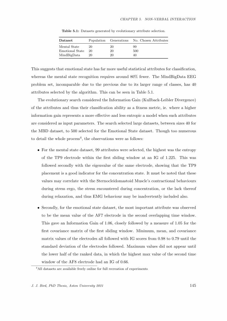
CHAPTER 5. NON-VERBAL INTERACTION
Table 5.1: Datasets generated by evolutionary attribute selection.
Dataset Population Generations No. Chosen Attributes
Mental State 20 20 99Emotional State 20 20 500MindBigData 20 20 40
This suggests that emotional state has far more useful statistical attributes for classification,
whereas the mental state recognition requires around 80% fewer. The MindBigData EEG
problem set, incomparable due to the previous due to its larger range of classes, has 40
attributes selected by the algorithm. This can be seen in Table 5.1.
The evolutionary search considered the Information Gain (Kullback-Leibler Divergence)
of the attributes and thus their classification ability as a fitness metric, ie. where a higher
information gain represents a more effective and less entropic a model when such attributes
are considered as input parameters. The search selected large datasets, between sizes 40 for
the MBD dataset, to 500 selected for the Emotional State dataset. Though too numerous
to detail the whole process4, the observations were as follows:
• For the mental state dataset, 99 attributes were selected, the highest was the entropy
of the TP9 electrode within the first sliding window at an IG of 1.225. This was
followed secondly with the eigenvalue of the same electrode, showing that the TP9
placement is a good indicator for the concentration state. It must be noted that these
values may correlate with the Sternocleidomastoid Muscle’s contractional behaviours
during stress ergo, the stress encountered during concentration, or the lack thereof
during relaxation, and thus EMG behaviour may be inadvertently included also.
• Secondly, for the emotional state dataset, the most important attribute was observed
to be the mean value of the AF7 electrode in the second overlapping time window.
This gave an Information Gain of 1.06, closely followed by a measure of 1.05 for the
first covariance matrix of the first sliding window. Minimum, mean, and covariance
matrix values of the electrodes all followed with IG scores from 0.98 to 0.79 until the
standard deviation of the electrodes followed. Maximum values did not appear until
the lower half of the ranked data, in which the highest max value of the second time
window of the AF8 electrode had an IG of 0.66.
4All datasets are available freely online for full recreation of experiments
J. J. Bird, PhD Thesis, Aston University 2021 145
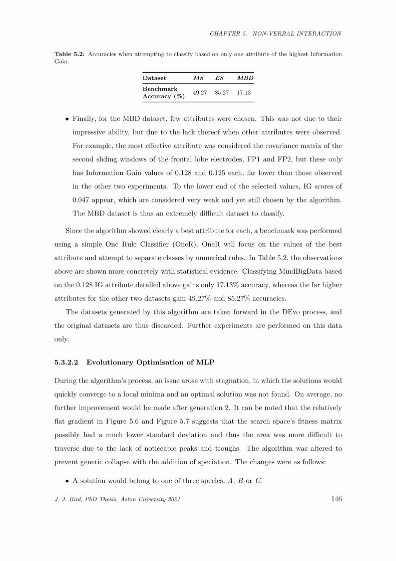
CHAPTER 5. NON-VERBAL INTERACTION
Table 5.2: Accuracies when attempting to classify based on only one attribute of the highest InformationGain.
Dataset MS ES MBD
BenchmarkAccuracy (%)
49.27 85.27 17.13
• Finally, for the MBD dataset, few attributes were chosen. This was not due to their
impressive ability, but due to the lack thereof when other attributes were observed.
For example, the most effective attribute was considered the covariance matrix of the
second sliding windows of the frontal lobe electrodes, FP1 and FP2, but these only
has Information Gain values of 0.128 and 0.125 each, far lower than those observed
in the other two experiments. To the lower end of the selected values, IG scores of
0.047 appear, which are considered very weak and yet still chosen by the algorithm.
The MBD dataset is thus an extremely difficult dataset to classify.
Since the algorithm showed clearly a best attribute for each, a benchmark was performed
using a simple One Rule Classifier (OneR). OneR will focus on the values of the best
attribute and attempt to separate classes by numerical rules. In Table 5.2, the observations
above are shown more concretely with statistical evidence. Classifying MindBigData based
on the 0.128 IG attribute detailed above gains only 17.13% accuracy, whereas the far higher
attributes for the other two datasets gain 49.27% and 85.27% accuracies.
The datasets generated by this algorithm are taken forward in the DEvo process, and
the original datasets are thus discarded. Further experiments are performed on this data
only.
5.3.2.2 Evolutionary Optimisation of MLP
During the algorithm’s process, an issue arose with stagnation, in which the solutions would
quickly converge to a local minima and an optimal solution was not found. On average, no
further improvement would be made after generation 2. It can be noted that the relatively
flat gradient in Figure 5.6 and Figure 5.7 suggests that the search space’s fitness matrix
possibly had a much lower standard deviation and thus the area was more difficult to
traverse due to the lack of noticeable peaks and troughs. The algorithm was altered to
prevent genetic collapse with the addition of speciation. The changes were as follows:
• A solution would belong to one of three species, A, B or C.
J. J. Bird, PhD Thesis, Aston University 2021 146
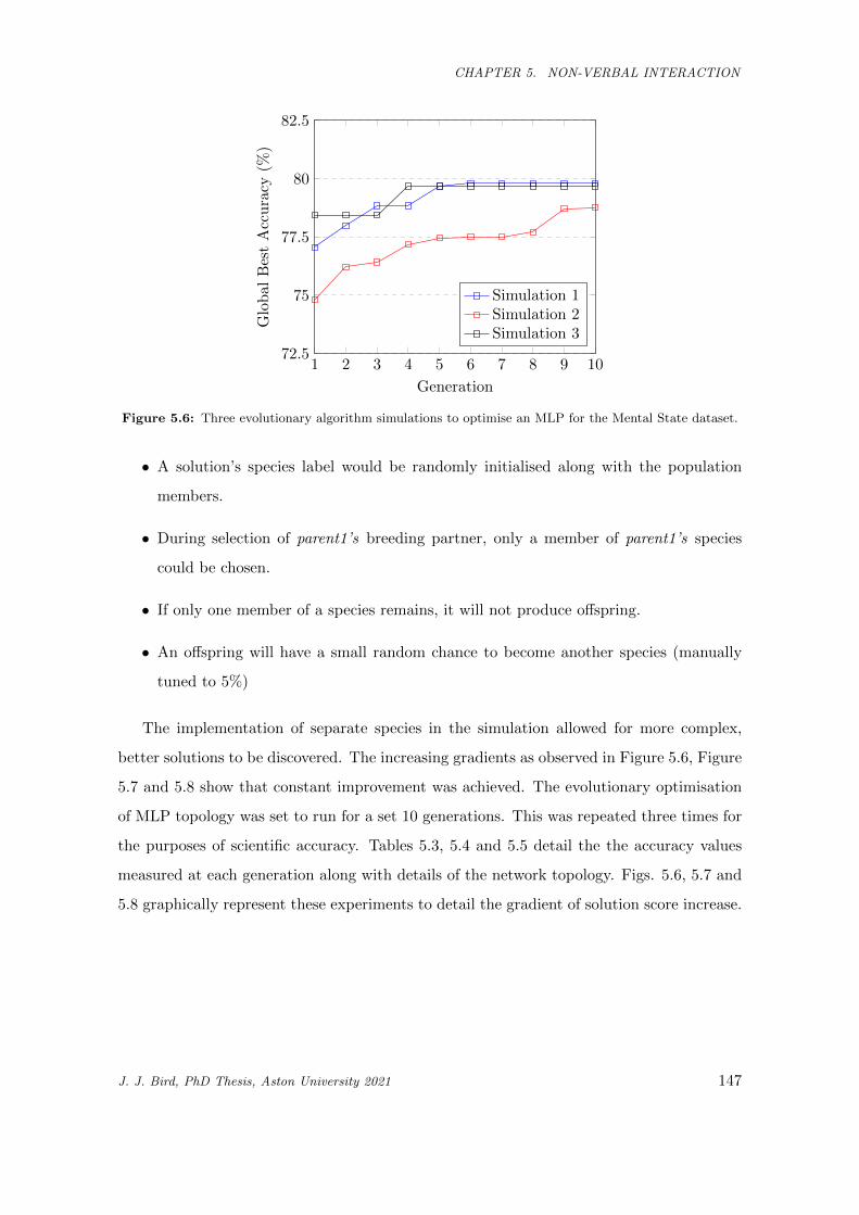
CHAPTER 5. NON-VERBAL INTERACTION
1 2 3 4 5 6 7 8 9 1072.5
75
77.5
80
82.5
Generation
Global
BestAccuracy
(%)
Simulation 1Simulation 2Simulation 3
Figure 5.6: Three evolutionary algorithm simulations to optimise an MLP for the Mental State dataset.
• A solution’s species label would be randomly initialised along with the population
members.
• During selection of parent1’s breeding partner, only a member of parent1’s species
could be chosen.
• If only one member of a species remains, it will not produce offspring.
• An offspring will have a small random chance to become another species (manually
tuned to 5%)
The implementation of separate species in the simulation allowed for more complex,
better solutions to be discovered. The increasing gradients as observed in Figure 5.6, Figure
5.7 and 5.8 show that constant improvement was achieved. The evolutionary optimisation
of MLP topology was set to run for a set 10 generations. This was repeated three times for
the purposes of scientific accuracy. Tables 5.3, 5.4 and 5.5 detail the the accuracy values
measured at each generation along with details of the network topology. Figs. 5.6, 5.7 and
5.8 graphically represent these experiments to detail the gradient of solution score increase.
J. J. Bird, PhD Thesis, Aston University 2021 147
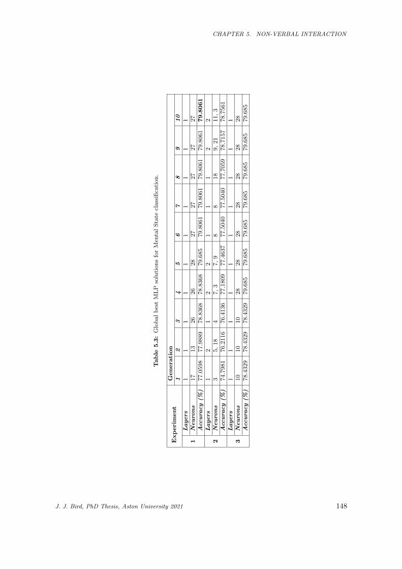
CHAPTER 5. NON-VERBAL INTERACTION
Table
5.3:
Glo
bal
bes
tM
LP
solu
tion
sfo
rM
enta
lS
tate
class
ifica
tion
.
Experiment
Genera
tion
12
34
56
78
910
1Layers
11
11
11
11
11
Neuro
ns
17
13
26
26
28
27
27
27
27
27
Acc
ura
cy(%
)77.0
598
77.9
889
78.8
368
78.8
368
79.6
85
79.8
061
79.8
061
79.8
061
79.8
061
79.8061
2Layers
12
12
21
11
22
Neuro
ns
35,
18
47,
37,
98
818
9,
21
11,
3Acc
ura
cy(%
)74.7
981
76.2
116
76.4
136
77.1
809
77.4
637
77.5
040
77.5
040
77.7
059
78.7
157
78.7
561
3Layers
11
11
11
11
11
Neuro
ns
10
10
10
28
28
28
28
28
28
28
Acc
ura
cy(%
)78.4
329
78.4
329
78.4
329
79.6
85
79.6
85
79.6
85
79.6
85
79.6
85
79.6
85
79.6
85
J. J. Bird, PhD Thesis, Aston University 2021 148
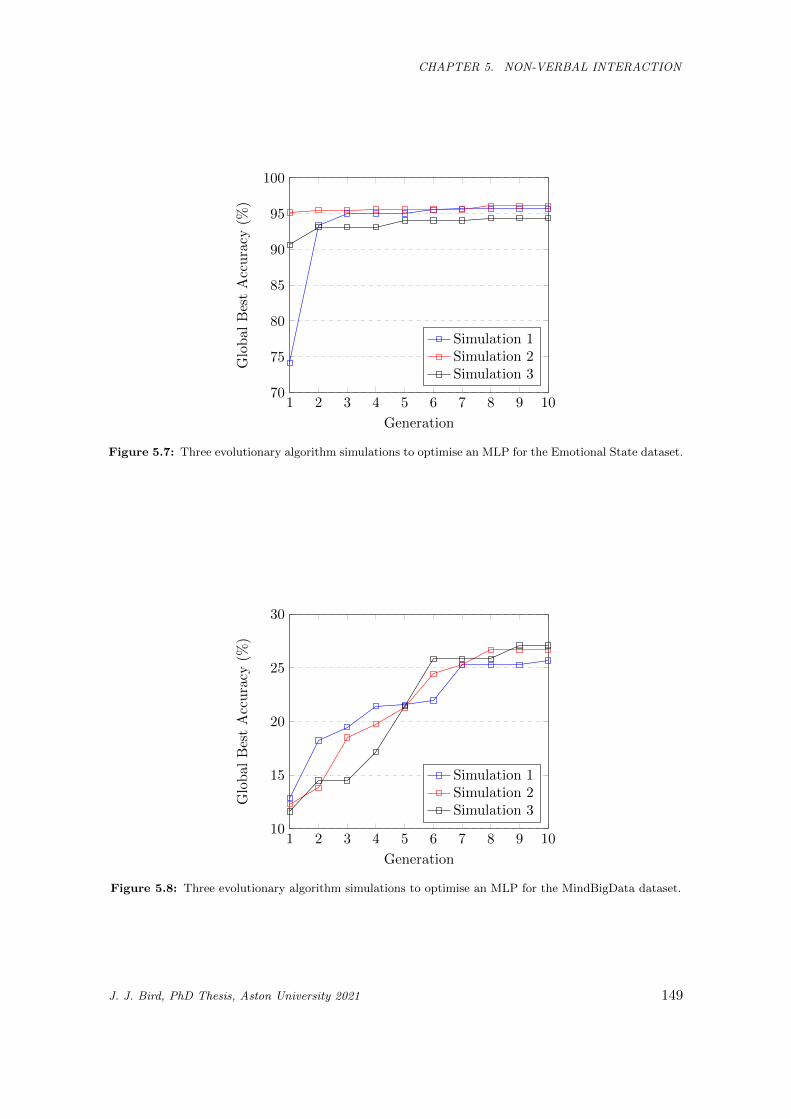
CHAPTER 5. NON-VERBAL INTERACTION
1 2 3 4 5 6 7 8 9 1070
75
80
85
90
95
100
Generation
Global
BestAccuracy
(%)
Simulation 1Simulation 2Simulation 3
Figure 5.7: Three evolutionary algorithm simulations to optimise an MLP for the Emotional State dataset.
1 2 3 4 5 6 7 8 9 1010
15
20
25
30
Generation
Global
BestAccuracy
(%)
Simulation 1Simulation 2Simulation 3
Figure 5.8: Three evolutionary algorithm simulations to optimise an MLP for the MindBigData dataset.
J. J. Bird, PhD Thesis, Aston University 2021 149
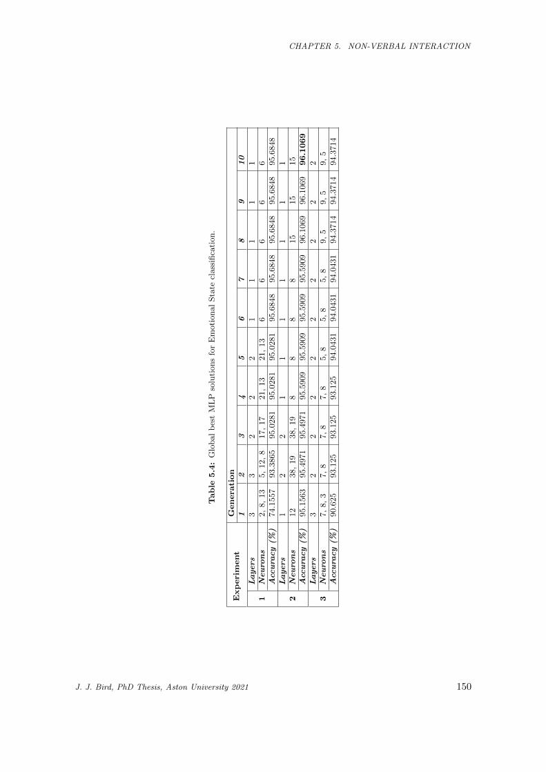
CHAPTER 5. NON-VERBAL INTERACTION
Table
5.4:
Glo
bal
bes
tM
LP
solu
tion
sfo
rE
moti
on
al
Sta
tecl
ass
ifica
tion
.
Experiment
Genera
tion
12
34
56
78
910
1Layers
33
22
21
11
11
Neuro
ns
2,
8,
13
5,
12,
817,
17
21,
13
21,
13
66
66
6Acc
ura
cy(%
)74.1
557
93.3
865
95.0
281
95.0
281
95.0
281
95.6
848
95.6
848
95.6
848
95.6
848
95.6
848
2Layers
12
21
11
11
11
Neuro
ns
12
38,
19
38,
19
88
88
15
15
15
Acc
ura
cy(%
)95.1
563
95.4
971
95.4
971
95.5
909
95.5
909
95.5
909
95.5
909
96.1
069
96.1
069
96.1069
3Layers
32
22
22
22
22
Neuro
ns
7,
8,
37,
87,
87,
85,
85,
85,
89,
59,
59,
5Acc
ura
cy(%
)90.6
25
93.1
25
93.1
25
93.1
25
94.0
431
94.0
431
94.0
431
94.3
714
94.3
714
94.3
714
J. J. Bird, PhD Thesis, Aston University 2021 150
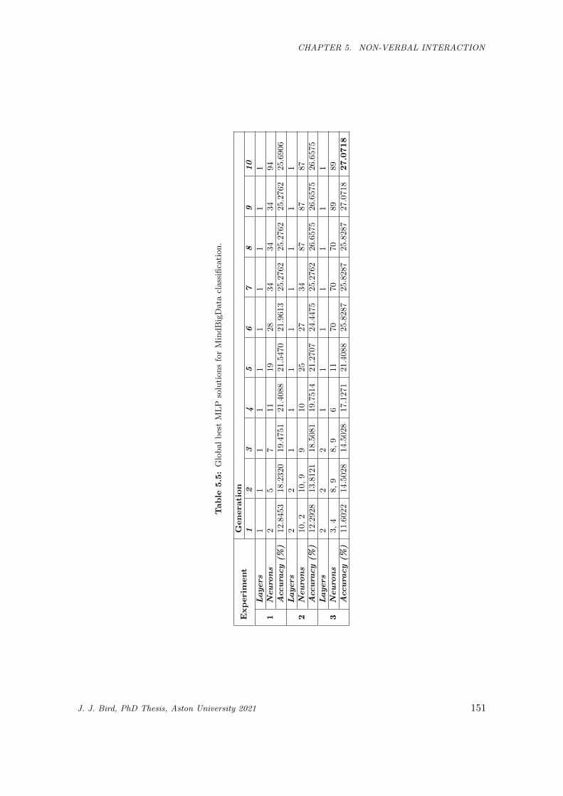
CHAPTER 5. NON-VERBAL INTERACTION
Table
5.5:
Glo
bal
bes
tM
LP
solu
tion
sfo
rM
ind
Big
Data
class
ifica
tion
.
Experiment
Genera
tion
12
34
56
78
910
1Layers
11
11
11
11
11
Neuro
ns
25
711
19
28
34
34
34
94
Acc
ura
cy(%
)12.8
453
18.2
320
19.4
751
21.4
088
21.5
470
21.9
613
25.2
762
25.2
762
25.2
762
25.6
906
2Layers
22
11
11
11
11
Neuro
ns
10,
210,
99
10
25
27
34
87
87
87
Acc
ura
cy(%
)12.2
928
13.8
121
18.5
081
19.7
514
21.2
707
24.4
475
25.2
762
26.6
575
26.6
575
26.6
575
3Layers
22
21
11
11
11
Neuro
ns
3,
48,
98,
96
11
70
70
70
89
89
Acc
ura
cy(%
)11.6
022
14.5
028
14.5
028
17.1
271
21.4
088
25.8
287
25.8
287
25.8
287
27.0
718
27.0718
J. J. Bird, PhD Thesis, Aston University 2021 151
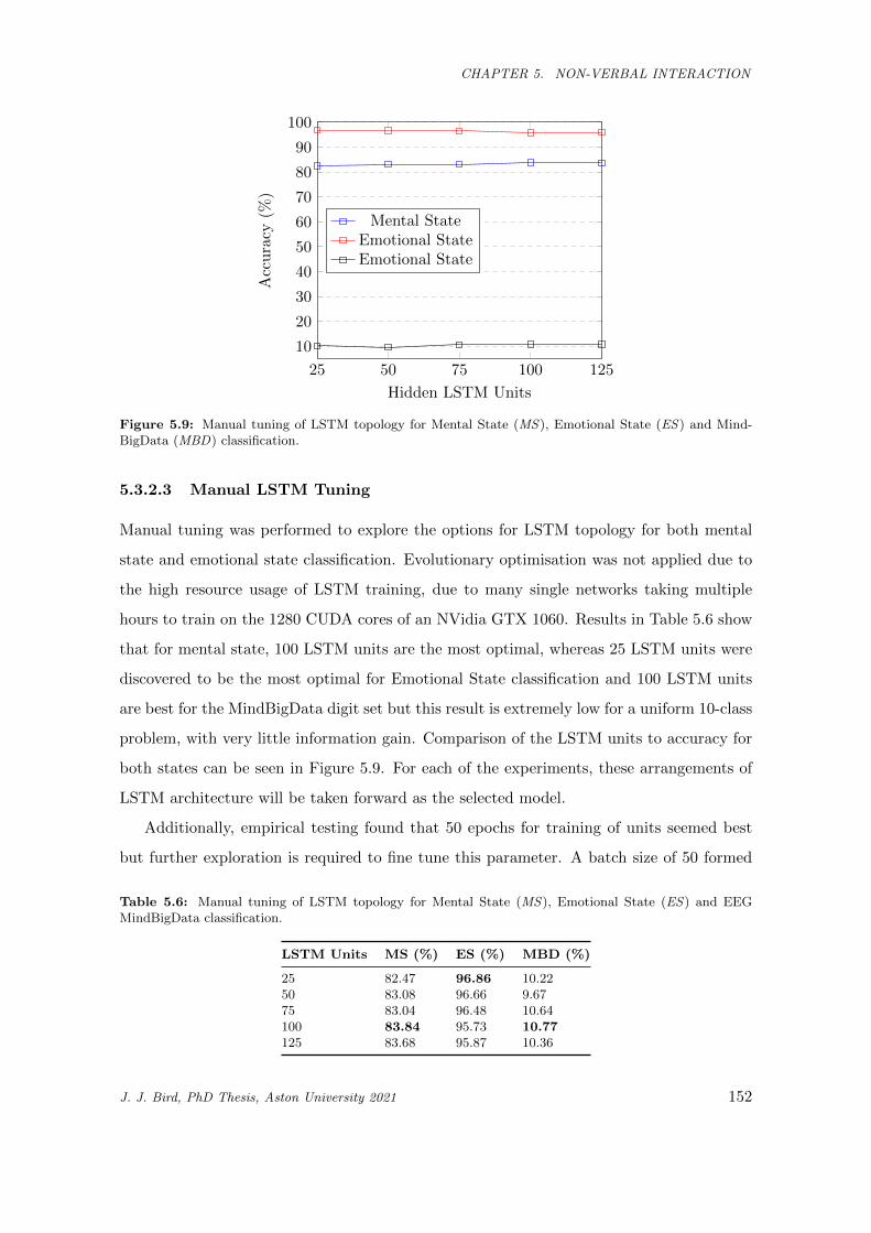
CHAPTER 5. NON-VERBAL INTERACTION
25 50 75 100 125
10
20
30
40
50
60
70
80
90
100
Hidden LSTM Units
Accuracy
(%)
Mental StateEmotional StateEmotional State
Figure 5.9: Manual tuning of LSTM topology for Mental State (MS), Emotional State (ES) and Mind-BigData (MBD) classification.
5.3.2.3 Manual LSTM Tuning
Manual tuning was performed to explore the options for LSTM topology for both mental
state and emotional state classification. Evolutionary optimisation was not applied due to
the high resource usage of LSTM training, due to many single networks taking multiple
hours to train on the 1280 CUDA cores of an NVidia GTX 1060. Results in Table 5.6 show
that for mental state, 100 LSTM units are the most optimal, whereas 25 LSTM units were
discovered to be the most optimal for Emotional State classification and 100 LSTM units
are best for the MindBigData digit set but this result is extremely low for a uniform 10-class
problem, with very little information gain. Comparison of the LSTM units to accuracy for
both states can be seen in Figure 5.9. For each of the experiments, these arrangements of
LSTM architecture will be taken forward as the selected model.
Additionally, empirical testing found that 50 epochs for training of units seemed best
but further exploration is required to fine tune this parameter. A batch size of 50 formed
Table 5.6: Manual tuning of LSTM topology for Mental State (MS), Emotional State (ES) and EEGMindBigData classification.
LSTM Units MS (%) ES (%) MBD (%)
25 82.47 96.86 10.2250 83.08 96.66 9.6775 83.04 96.48 10.64100 83.84 95.73 10.77125 83.68 95.87 10.36
J. J. Bird, PhD Thesis, Aston University 2021 152
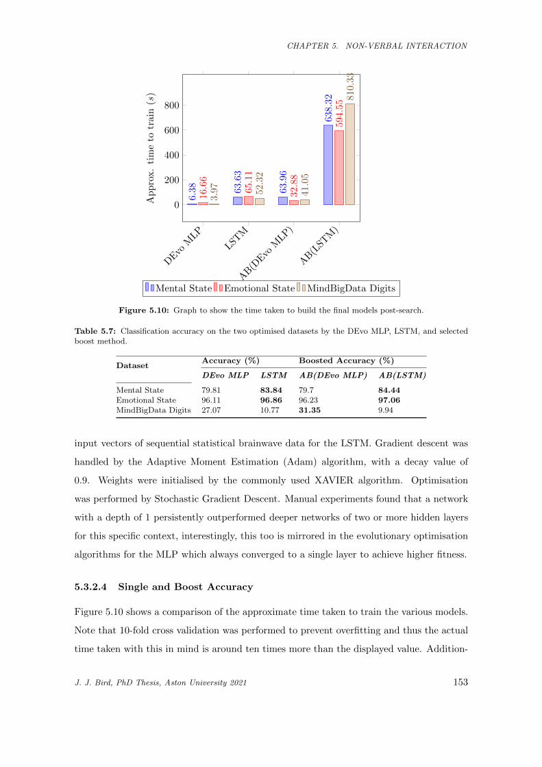
CHAPTER 5. NON-VERBAL INTERACTION
DEvoMLP
LSTM
AB(DEvoMLP)
AB(LSTM)
0
200
400
600
800
6.38
63.63
63.96
638.32
16.66
65.11
32.88
594.55
3.97
52.32
41.05
810
.33
Approx.timeto
train
(s)
Mental State Emotional State MindBigData Digits
Figure 5.10: Graph to show the time taken to build the final models post-search.
Table 5.7: Classification accuracy on the two optimised datasets by the DEvo MLP, LSTM, and selectedboost method.
DatasetAccuracy (%) Boosted Accuracy (%)
DEvo MLP LSTM AB(DEvo MLP) AB(LSTM)
Mental State 79.81 83.84 79.7 84.44Emotional State 96.11 96.86 96.23 97.06MindBigData Digits 27.07 10.77 31.35 9.94
input vectors of sequential statistical brainwave data for the LSTM. Gradient descent was
handled by the Adaptive Moment Estimation (Adam) algorithm, with a decay value of
0.9. Weights were initialised by the commonly used XAVIER algorithm. Optimisation
was performed by Stochastic Gradient Descent. Manual experiments found that a network
with a depth of 1 persistently outperformed deeper networks of two or more hidden layers
for this specific context, interestingly, this too is mirrored in the evolutionary optimisation
algorithms for the MLP which always converged to a single layer to achieve higher fitness.
5.3.2.4 Single and Boost Accuracy
Figure 5.10 shows a comparison of the approximate time taken to train the various models.
Note that 10-fold cross validation was performed to prevent overfitting and thus the actual
time taken with this in mind is around ten times more than the displayed value. Addition-
J. J. Bird, PhD Thesis, Aston University 2021 153
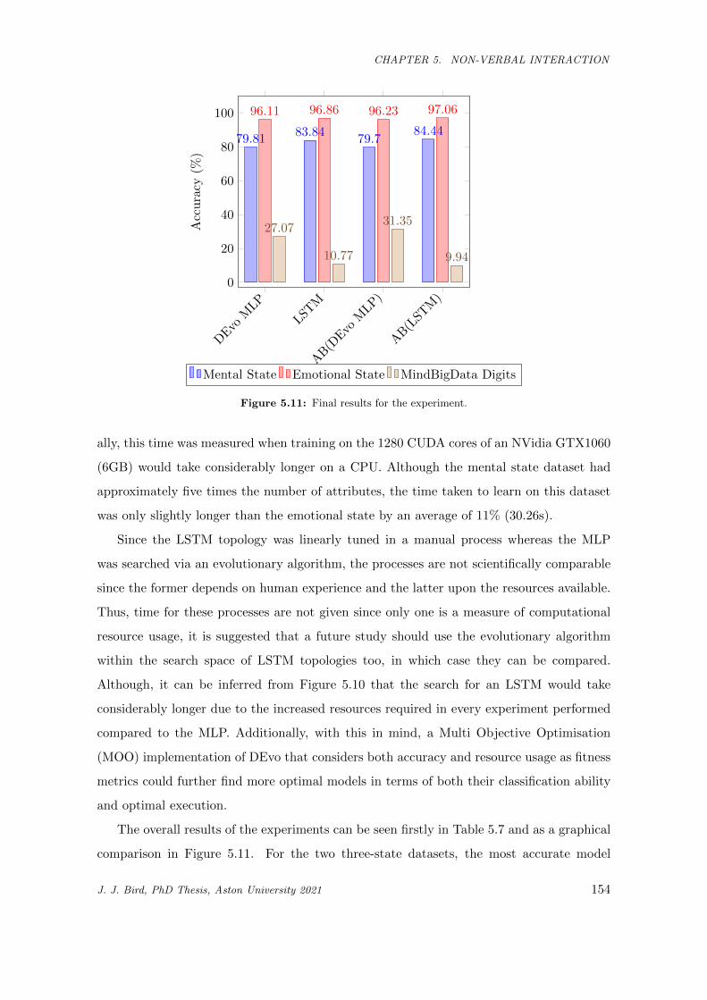
CHAPTER 5. NON-VERBAL INTERACTION
DEvoMLP
LSTM
AB(DEvoMLP)
AB(LSTM)
0
20
40
60
80
100
79.8183.84
79.784.44
96.11 96.86 96.23 97.06
27.07
10.77
31.35
9.94
Accuracy
(%)
Mental State Emotional State MindBigData Digits
Figure 5.11: Final results for the experiment.
ally, this time was measured when training on the 1280 CUDA cores of an NVidia GTX1060
(6GB) would take considerably longer on a CPU. Although the mental state dataset had
approximately five times the number of attributes, the time taken to learn on this dataset
was only slightly longer than the emotional state by an average of 11% (30.26s).
Since the LSTM topology was linearly tuned in a manual process whereas the MLP
was searched via an evolutionary algorithm, the processes are not scientifically comparable
since the former depends on human experience and the latter upon the resources available.
Thus, time for these processes are not given since only one is a measure of computational
resource usage, it is suggested that a future study should use the evolutionary algorithm
within the search space of LSTM topologies too, in which case they can be compared.
Although, it can be inferred from Figure 5.10 that the search for an LSTM would take
considerably longer due to the increased resources required in every experiment performed
compared to the MLP. Additionally, with this in mind, a Multi Objective Optimisation
(MOO) implementation of DEvo that considers both accuracy and resource usage as fitness
metrics could further find more optimal models in terms of both their classification ability
and optimal execution.
The overall results of the experiments can be seen firstly in Table 5.7 and as a graphical
comparison in Figure 5.11. For the two three-state datasets, the most accurate model
J. J. Bird, PhD Thesis, Aston University 2021 154
CHAPTER 5. NON-VERBAL INTERACTION
was an AdaBoosted LSTM with results of 84.44% and 97.06% accuracies for the mental
state and mental emotional state datasets respectively. The single LSTM and Evolutionary
Optimised MLP models come relatively close to the best result, though take far less time
to train when the measured approximate values in Figure 5.10 are observed. On the other
hand, for the MindBigData digits dataset, the best solution by far was the Adaptive Boosted
DEvo MLP, and the same boosting method applied to the LSTM that previously improved
them, actually caused a loss in accuracy.
Manual tuning of LSTM network topology was performed due to the limited compu-
tational resources available, the success in optimisation of the MLP suggests further im-
provements could be made through an automated process of evolutionary optimisation in
terms of the LSTM topology. A further improvement to the DEvo system could be made
by exploring the possibility of optimising the LSTM structure through an evolutionary
approach.
The three experiments were performed within the limitations of the Muse headband’s
TP9, AF7, AF8, and TP10 electrodes. Higher resolution EEG setups would allow for further
exploration of the system in terms of mental data classification, e.g., for physical movement
originating from the motor cortex.
5.4 CNN Classification of EEG Signals represented in 2D
and 3D
The novelty of this study consists of the exploration of multiple new approaches of data
pre-processing of brainwave signals, wherein statistical features are extracted and then
formatted as visual images based on the order in which dimensionality reduction algorithms
select them. This data is then treated as a visual input for 2D and 3D CNNs which further
extract ‘features of features’. Statistical features derived from three electroencephalography
datasets are presented in visual space and processed in 2D and 3D space as pixels and
voxels respectively. Three datasets are benchmarked, mental attention states and emotional
valences from the four TP9, AF7, AF8 and TP10 10-20 electrodes and an eye state data
from 64 electrodes. 729 features are selected through three methods of selection in order to
form 27x27 images and 9x9x9 cubes from the same dataset. CNNs engineered for the 2D
and 3D preprocessing representations learn to convolve useful graphical features from the
J. J. Bird, PhD Thesis, Aston University 2021 155
CHAPTER 5. NON-VERBAL INTERACTION
data.
Recent advances in consumer-facing technologies have enabled machines to have non-
human skills. Inputs which once mirrored one’s natural senses such as vision and sound
have been expanded beyond the natural realms. An important example of this is the grow-
ing consumerist availability of the field of electroencephalography (EEG); the detection
of thoughts, actions, and feelings from the human brain. To engineer such technologies,
researchers must consider the actual format of the data itself as input to the machine or
deep learning models, which subsequently develop the ability to distinguish between these
nominal thought patterns. Usually, this is either statistically 1-Dimensional or temporally
2-Dimensional since there is an extra consideration of time and sequence. Due to the avail-
ability of resources in the modern day, a more enabled area of research into a new formatting
technique is graphical representation, i.e., presenting 1-Dimensional mathematical descrip-
tors of waves in multiple spatial dimensions in order to form an image or model in Euclidean
space. This format of data can then be further represented by feature maps from convolu-
tional operations. With preliminary success of the approach, a deeper understanding must
be sought in order to distinguish in which spatial dimension brainwave signals are most apt
for interpretation. With the classical method of raw wave data being used as input to a
CNN in mind, dimensionality reduction is especially difficult given the often blackbox-like
nature of a CNNs internal feature extraction processes. In this work, statistical temporal
features are extracted from the waves which serve as input to the CNN, which allows for
direct control of input complexity since dimensionality reduction can be used to choose
the best n features within the set with the task in mind. Reduction of a CNN topology,
whether that be network depth or layer width, gives less control over which features are
and are not computed. Given the technique of feature extraction as input to the CNN, and
thus the aforementioned direct control of input complexity, reduction of CNN complexity
reduces the number of ‘features of features’ computed; that is, all chosen input attributes
are retained.
In this work, an experimental framework is presented in which the evolutionary optimisa-
tion of neural network hyperparameters is applied in conjunction with a visual data prepro-
cessing technique. This work explores visual data reshaping in 2 and 3 dimensions to form
pixel image and voxel cube representations of statistical features extracted from electrical
brain activity, through which 2D and 3D CNN convolve ‘features of features’. In addition,
J. J. Bird, PhD Thesis, Aston University 2021 156
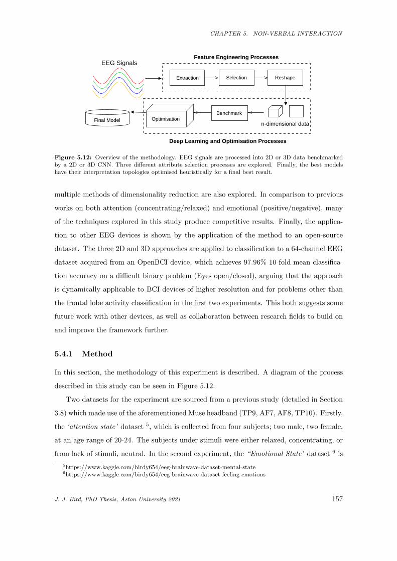
CHAPTER 5. NON-VERBAL INTERACTION
EEG Signals
Extraction Selection Reshape
n-dimensional data
BenchmarkOptimisationFinal Model
Feature Engineering Processes
Deep Learning and Optimisation Processes
Figure 5.12: Overview of the methodology. EEG signals are processed into 2D or 3D data benchmarkedby a 2D or 3D CNN. Three different attribute selection processes are explored. Finally, the best modelshave their interpretation topologies optimised heuristically for a final best result.
multiple methods of dimensionality reduction are also explored. In comparison to previous
works on both attention (concentrating/relaxed) and emotional (positive/negative), many
of the techniques explored in this study produce competitive results. Finally, the applica-
tion to other EEG devices is shown by the application of the method to an open-source
dataset. The three 2D and 3D approaches are applied to classification to a 64-channel EEG
dataset acquired from an OpenBCI device, which achieves 97.96% 10-fold mean classifica-
tion accuracy on a difficult binary problem (Eyes open/closed), arguing that the approach
is dynamically applicable to BCI devices of higher resolution and for problems other than
the frontal lobe activity classification in the first two experiments. This both suggests some
future work with other devices, as well as collaboration between research fields to build on
and improve the framework further.
5.4.1 Method
In this section, the methodology of this experiment is described. A diagram of the process
described in this study can be seen in Figure 5.12.
Two datasets for the experiment are sourced from a previous study (detailed in Section
3.8) which made use of the aforementioned Muse headband (TP9, AF7, AF8, TP10). Firstly,
the ‘attention state’ dataset 5, which is collected from four subjects; two male, two female,
at an age range of 20-24. The subjects under stimuli were either relaxed, concentrating, or
from lack of stimuli, neutral. In the second experiment, the “Emotional State’ dataset 6 is
5https://www.kaggle.com/birdy654/eeg-brainwave-dataset-mental-state6https://www.kaggle.com/birdy654/eeg-brainwave-dataset-feeling-emotions
J. J. Bird, PhD Thesis, Aston University 2021 157
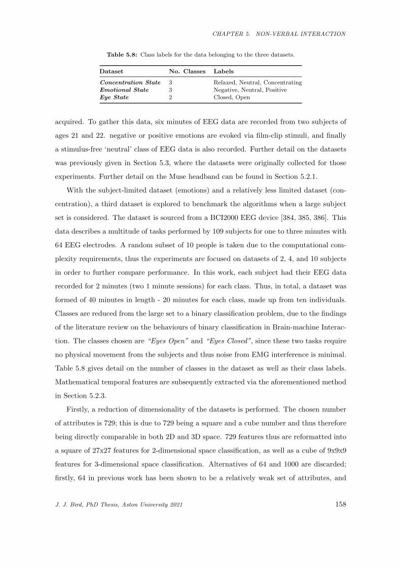
CHAPTER 5. NON-VERBAL INTERACTION
Table 5.8: Class labels for the data belonging to the three datasets.
Dataset No. Classes Labels
Concentration State 3 Relaxed, Neutral, ConcentratingEmotional State 3 Negative, Neutral, PositiveEye State 2 Closed, Open
acquired. To gather this data, six minutes of EEG data are recorded from two subjects of
ages 21 and 22. negative or positive emotions are evoked via film-clip stimuli, and finally
a stimulus-free ‘neutral’ class of EEG data is also recorded. Further detail on the datasets
was previously given in Section 5.3, where the datasets were originally collected for those
experiments. Further detail on the Muse headband can be found in Section 5.2.1.
With the subject-limited dataset (emotions) and a relatively less limited dataset (con-
centration), a third dataset is explored to benchmark the algorithms when a large subject
set is considered. The dataset is sourced from a BCI2000 EEG device [384, 385, 386]. This
data describes a multitude of tasks performed by 109 subjects for one to three minutes with
64 EEG electrodes. A random subset of 10 people is taken due to the computational com-
plexity requirements, thus the experiments are focused on datasets of 2, 4, and 10 subjects
in order to further compare performance. In this work, each subject had their EEG data
recorded for 2 minutes (two 1 minute sessions) for each class. Thus, in total, a dataset was
formed of 40 minutes in length - 20 minutes for each class, made up from ten individuals.
Classes are reduced from the large set to a binary classification problem, due to the findings
of the literature review on the behaviours of binary classification in Brain-machine Interac-
tion. The classes chosen are “Eyes Open” and “Eyes Closed”, since these two tasks require
no physical movement from the subjects and thus noise from EMG interference is minimal.
Table 5.8 gives detail on the number of classes in the dataset as well as their class labels.
Mathematical temporal features are subsequently extracted via the aforementioned method
in Section 5.2.3.
Firstly, a reduction of dimensionality of the datasets is performed. The chosen number
of attributes is 729; this is due to 729 being a square and a cube number and thus therefore
being directly comparable in both 2D and 3D space. 729 features thus are reformatted into
a square of 27x27 features for 2-dimensional space classification, as well as a cube of 9x9x9
features for 3-dimensional space classification. Alternatives of 64 and 1000 are discarded;
firstly, 64 in previous work has been shown to be a relatively weak set of attributes, and
J. J. Bird, PhD Thesis, Aston University 2021 158
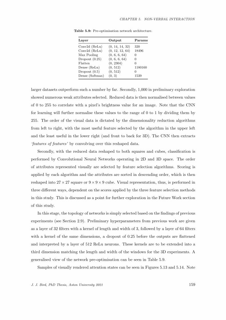
CHAPTER 5. NON-VERBAL INTERACTION
Table 5.9: Pre-optimisation network architecture.
Layer Output Params
Conv2d (ReLu) (0, 14, 14, 32) 320Conv2d (ReLu) (0, 12, 12, 64) 18496Max Pooling (0, 6, 6, 64) 0Dropout (0.25) (0, 6, 6, 64) 0Flatten (0, 2304) 0Dense (ReLu) (0, 512) 1180160Dropout (0.5) (0, 512) 0Dense (Softmax) (0, 3) 1539
larger datasets outperform such a number by far. Secondly, 1,000 in preliminary exploration
showed numerous weak attributes selected. Reduced data is then normalised between values
of 0 to 255 to correlate with a pixel’s brightness value for an image. Note that the CNN
for learning will further normalise these values to the range of 0 to 1 by dividing them by
255. The order of the visual data is dictated by the dimensionality reduction algorithms
from left to right, with the most useful feature selected by the algorithm in the upper left
and the least useful in the lower right (and front to back for 3D). The CNN then extracts
‘features of features’ by convolving over this reshaped data.
Secondly, with the reduced data reshaped to both squares and cubes, classification is
performed by Convolutional Neural Networks operating in 2D and 3D space. The order
of attributes represented visually are selected by feature selection algorithms. Scoring is
applied by each algorithm and the attributes are sorted in descending order, which is then
reshaped into 27× 27 square or 9× 9× 9 cube. Visual representation, thus, is performed in
three different ways, dependent on the scores applied by the three feature selection methods
in this study. This is discussed as a point for further exploration in the Future Work section
of this study.
In this stage, the topology of networks is simply selected based on the findings of previous
experiments (see Section 2.9). Preliminary hyperparameters from previous work are given
as a layer of 32 filters with a kernel of length and width of 3, followed by a layer of 64 filters
with a kernel of the same dimensions, a dropout of 0.25 before the outputs are flattened
and interpreted by a layer of 512 ReLu neurons. These kernels are to be extended into a
third dimension matching the length and width of the windows for the 3D experiments. A
generalised view of the network pre-optimisation can be seen in Table 5.9.
Samples of visually rendered attention states can be seen in Figures 5.13 and 5.14. Note
J. J. Bird, PhD Thesis, Aston University 2021 159
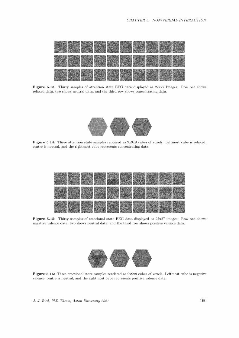
CHAPTER 5. NON-VERBAL INTERACTION
Figure 5.13: Thirty samples of attention state EEG data displayed as 27x27 Images. Row one showsrelaxed data, two shows neutral data, and the third row shows concentrating data.
Figure 5.14: Three attention state samples rendered as 9x9x9 cubes of voxels. Leftmost cube is relaxed,centre is neutral, and the rightmost cube represents concentrating data.
Figure 5.15: Thirty samples of emotional state EEG data displayed as 27x27 images. Row one showsnegative valence data, two shows neutral data, and the third row shows positive valence data.
Figure 5.16: Three emotional state samples rendered as 9x9x9 cubes of voxels. Leftmost cube is negativevalence, centre is neutral, and the rightmost cube represents positive valence data.
J. J. Bird, PhD Thesis, Aston University 2021 160
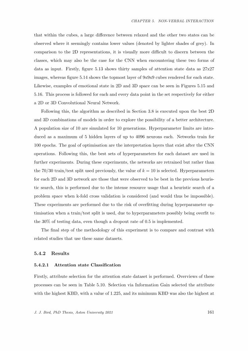
CHAPTER 5. NON-VERBAL INTERACTION
that within the cubes, a large difference between relaxed and the other two states can be
observed where it seemingly contains lower values (denoted by lighter shades of grey). In
comparison to the 2D representations, it is visually more difficult to discern between the
classes, which may also be the case for the CNN when encountering these two forms of
data as input. Firstly, figure 5.13 shows thirty samples of attention state data as 27x27
images, whereas figure 5.14 shows the topmost layer of 9x9x9 cubes rendered for each state.
Likewise, examples of emotional state in 2D and 3D space can be seen in Figures 5.15 and
5.16. This process is followed for each and every data point in the set respectively for either
a 2D or 3D Convolutional Neural Network.
Following this, the algorithm as described in Section 3.8 is executed upon the best 2D
and 3D combinations of models in order to explore the possibility of a better architecture.
A population size of 10 are simulated for 10 generations. Hyperparameter limits are intro-
duced as a maximum of 5 hidden layers of up to 4096 neurons each. Networks train for
100 epochs. The goal of optimisation are the interpretation layers that exist after the CNN
operations. Following this, the best sets of hyperparameters for each dataset are used in
further experiments. During these experiments, the networks are retrained but rather than
the 70/30 train/test split used previously, the value of k = 10 is selected. Hyperparameters
for each 2D and 3D network are those that were observed to be best in the previous heuris-
tic search, this is performed due to the intense resource usage that a heuristic search of a
problem space when k-fold cross validation is considered (and would thus be impossible).
These experiments are performed due to the risk of overfitting during hyperparameter op-
timisation when a train/test split is used, due to hyperparameters possibly being overfit to
the 30% of testing data, even though a dropout rate of 0.5 is implemented.
The final step of the methodology of this experiment is to compare and contrast with
related studies that use these same datasets.
5.4.2 Results
5.4.2.1 Attention state Classification
Firstly, attribute selection for the attention state dataset is performed. Overviews of these
processes can be seen in Table 5.10. Selection via Information Gain selected the attribute
with the highest KBD, with a value of 1.225, and its minimum KBD was also the highest at
J. J. Bird, PhD Thesis, Aston University 2021 161
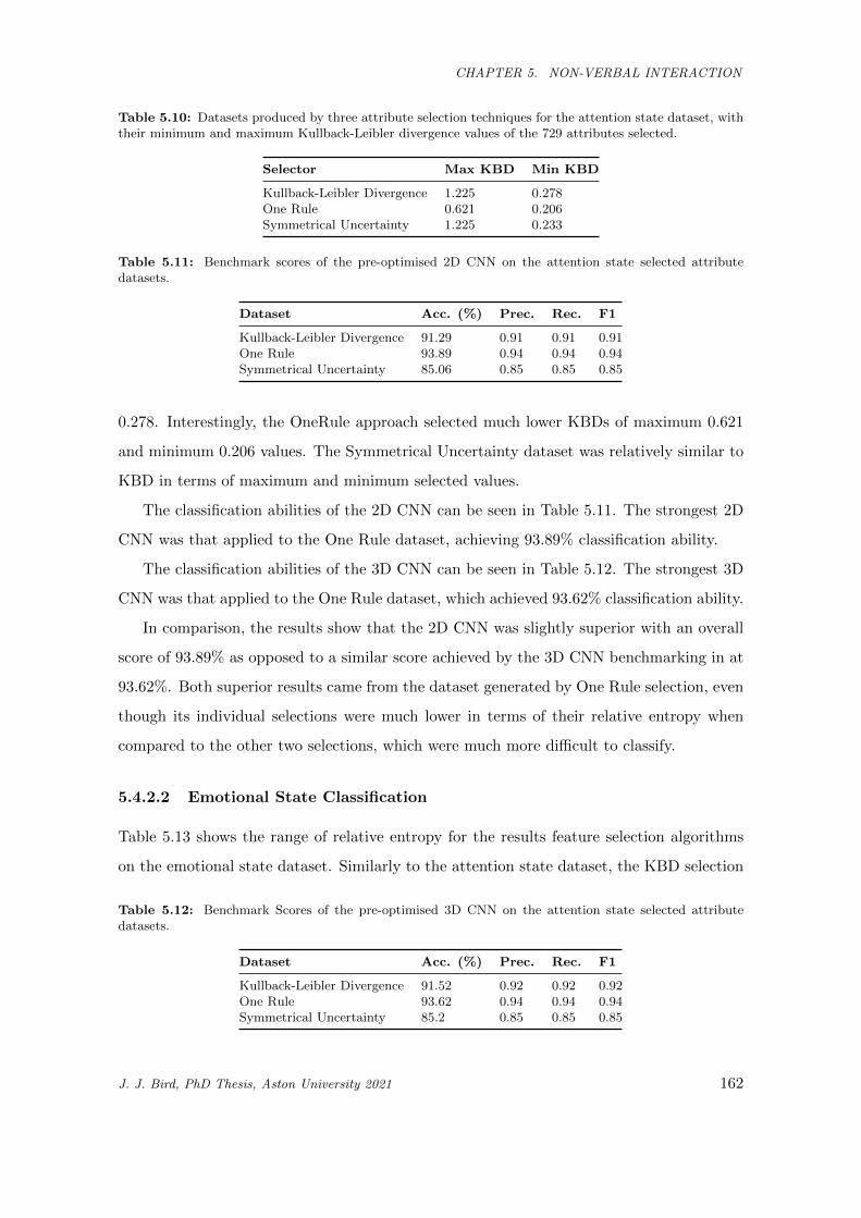
CHAPTER 5. NON-VERBAL INTERACTION
Table 5.10: Datasets produced by three attribute selection techniques for the attention state dataset, withtheir minimum and maximum Kullback-Leibler divergence values of the 729 attributes selected.
Selector Max KBD Min KBD
Kullback-Leibler Divergence 1.225 0.278One Rule 0.621 0.206Symmetrical Uncertainty 1.225 0.233
Table 5.11: Benchmark scores of the pre-optimised 2D CNN on the attention state selected attributedatasets.
Dataset Acc. (%) Prec. Rec. F1
Kullback-Leibler Divergence 91.29 0.91 0.91 0.91One Rule 93.89 0.94 0.94 0.94Symmetrical Uncertainty 85.06 0.85 0.85 0.85
0.278. Interestingly, the OneRule approach selected much lower KBDs of maximum 0.621
and minimum 0.206 values. The Symmetrical Uncertainty dataset was relatively similar to
KBD in terms of maximum and minimum selected values.
The classification abilities of the 2D CNN can be seen in Table 5.11. The strongest 2D
CNN was that applied to the One Rule dataset, achieving 93.89% classification ability.
The classification abilities of the 3D CNN can be seen in Table 5.12. The strongest 3D
CNN was that applied to the One Rule dataset, which achieved 93.62% classification ability.
In comparison, the results show that the 2D CNN was slightly superior with an overall
score of 93.89% as opposed to a similar score achieved by the 3D CNN benchmarking in at
93.62%. Both superior results came from the dataset generated by One Rule selection, even
though its individual selections were much lower in terms of their relative entropy when
compared to the other two selections, which were much more difficult to classify.
5.4.2.2 Emotional State Classification
Table 5.13 shows the range of relative entropy for the results feature selection algorithms
on the emotional state dataset. Similarly to the attention state dataset, the KBD selection
Table 5.12: Benchmark Scores of the pre-optimised 3D CNN on the attention state selected attributedatasets.
Dataset Acc. (%) Prec. Rec. F1
Kullback-Leibler Divergence 91.52 0.92 0.92 0.92One Rule 93.62 0.94 0.94 0.94Symmetrical Uncertainty 85.2 0.85 0.85 0.85
J. J. Bird, PhD Thesis, Aston University 2021 162
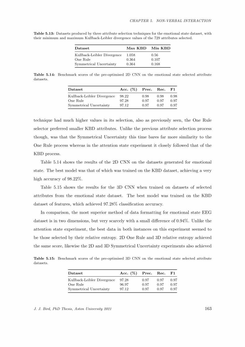
CHAPTER 5. NON-VERBAL INTERACTION
Table 5.13: Datasets produced by three attribute selection techniques for the emotional state dataset, withtheir minimum and maximum Kullback-Leibler divergence values of the 729 attributes selected.
Dataset Max KBD Min KBD
Kullback-Leibler Divergence 1.058 0.56One Rule 0.364 0.107Symmetrical Uncertainty 0.364 0.168
Table 5.14: Benchmark scores of the pre-optimised 2D CNN on the emotional state selected attributedatasets.
Dataset Acc. (%) Prec. Rec. F1
Kullback-Leibler Divergence 98.22 0.98 0.98 0.98One Rule 97.28 0.97 0.97 0.97Symmetrical Uncertainty 97.12 0.97 0.97 0.97
technique had much higher values in its selection, also as previously seen, the One Rule
selector preferred smaller KBD attributes. Unlike the previous attribute selection process
though, was that the Symmetrical Uncertainty this time bares far more similarity to the
One Rule process whereas in the attention state experiment it closely followed that of the
KBD process.
Table 5.14 shows the results of the 2D CNN on the datasets generated for emotional
state. The best model was that of which was trained on the KBD dataset, achieving a very
high accuracy of 98.22%.
Table 5.15 shows the results for the 3D CNN when trained on datasets of selected
attributes from the emotional state dataset. The best model was trained on the KBD
dataset of features, which achieved 97.28% classification accuracy.
In comparison, the most superior method of data formatting for emotional state EEG
dataset is in two dimensions, but very scarcely with a small difference of 0.94%. Unlike the
attention state experiment, the best data in both instances on this experiment seemed to
be those selected by their relative entropy. 2D One Rule and 3D relative entropy achieved
the same score, likewise the 2D and 3D Symmetrical Uncertainty experiments also achieved
Table 5.15: Benchmark scores of the pre-optimised 3D CNN on the emotional state selected attributedatasets.
Dataset Acc. (%) Prec. Rec. F1
Kullback-Leibler Divergence 97.28 0.97 0.97 0.97One Rule 96.97 0.97 0.97 0.97Symmetrical Uncertainty 97.12 0.97 0.97 0.97
J. J. Bird, PhD Thesis, Aston University 2021 163
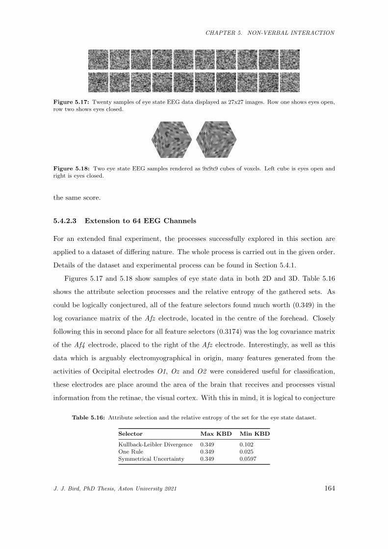
CHAPTER 5. NON-VERBAL INTERACTION
Figure 5.17: Twenty samples of eye state EEG data displayed as 27x27 images. Row one shows eyes open,row two shows eyes closed.
Figure 5.18: Two eye state EEG samples rendered as 9x9x9 cubes of voxels. Left cube is eyes open andright is eyes closed.
the same score.
5.4.2.3 Extension to 64 EEG Channels
For an extended final experiment, the processes successfully explored in this section are
applied to a dataset of differing nature. The whole process is carried out in the given order.
Details of the dataset and experimental process can be found in Section 5.4.1.
Figures 5.17 and 5.18 show samples of eye state data in both 2D and 3D. Table 5.16
shows the attribute selection processes and the relative entropy of the gathered sets. As
could be logically conjectured, all of the feature selectors found much worth (0.349) in the
log covariance matrix of the Afz electrode, located in the centre of the forehead. Closely
following this in second place for all feature selectors (0.3174) was the log covariance matrix
of the Af4 electrode, placed to the right of the Afz electrode. Interestingly, as well as this
data which is arguably electromyographical in origin, many features generated from the
activities of Occipital electrodes O1, Oz and O2 were considered useful for classification,
these electrodes are place around the area of the brain that receives and processes visual
information from the retinae, the visual cortex. With this in mind, it is logical to conjecture
Table 5.16: Attribute selection and the relative entropy of the set for the eye state dataset.
Selector Max KBD Min KBD
Kullback-Leibler Divergence 0.349 0.102One Rule 0.349 0.025Symmetrical Uncertainty 0.349 0.0597
J. J. Bird, PhD Thesis, Aston University 2021 164
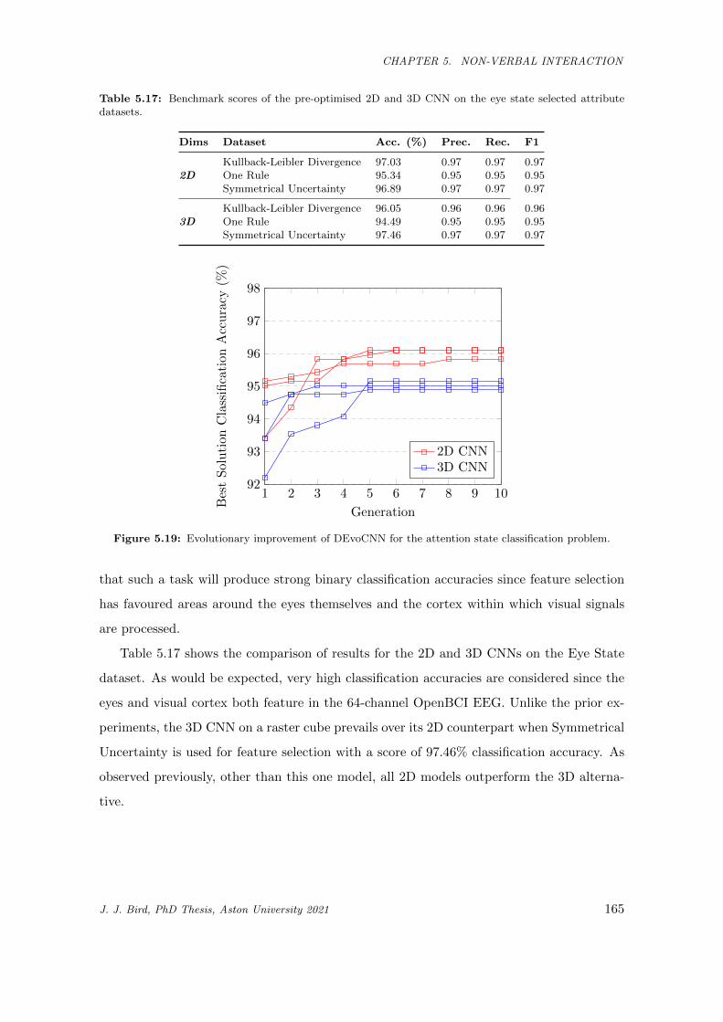
CHAPTER 5. NON-VERBAL INTERACTION
Table 5.17: Benchmark scores of the pre-optimised 2D and 3D CNN on the eye state selected attributedatasets.
Dims Dataset Acc. (%) Prec. Rec. F1
2DKullback-Leibler Divergence 97.03 0.97 0.97 0.97One Rule 95.34 0.95 0.95 0.95Symmetrical Uncertainty 96.89 0.97 0.97 0.97
3DKullback-Leibler Divergence 96.05 0.96 0.96 0.96One Rule 94.49 0.95 0.95 0.95Symmetrical Uncertainty 97.46 0.97 0.97 0.97
1 2 3 4 5 6 7 8 9 1092
93
94
95
96
97
98
Generation
BestSolution
ClassificationAccuracy
(%)
2D CNN3D CNN
Figure 5.19: Evolutionary improvement of DEvoCNN for the attention state classification problem.
that such a task will produce strong binary classification accuracies since feature selection
has favoured areas around the eyes themselves and the cortex within which visual signals
are processed.
Table 5.17 shows the comparison of results for the 2D and 3D CNNs on the Eye State
dataset. As would be expected, very high classification accuracies are considered since the
eyes and visual cortex both feature in the 64-channel OpenBCI EEG. Unlike the prior ex-
periments, the 3D CNN on a raster cube prevails over its 2D counterpart when Symmetrical
Uncertainty is used for feature selection with a score of 97.46% classification accuracy. As
observed previously, other than this one model, all 2D models outperform the 3D alterna-
tive.
J. J. Bird, PhD Thesis, Aston University 2021 165
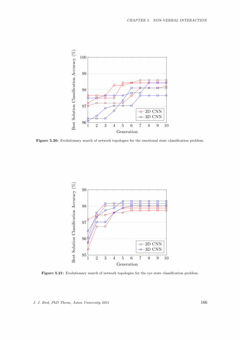
CHAPTER 5. NON-VERBAL INTERACTION
1 2 3 4 5 6 7 8 9 1096
97
98
99
100
Generation
BestSolutionClassification
Accuracy
(%)
2D CNN3D CNN
Figure 5.20: Evolutionary search of network topologies for the emotional state classification problem.
1 2 3 4 5 6 7 8 9 1095
96
97
98
99
Generation
BestSolutionClassification
Accuracy
(%)
2D CNN3D CNN
Figure 5.21: Evolutionary search of network topologies for the eye state classification problem.
J. J. Bird, PhD Thesis, Aston University 2021 166
CHAPTER 5. NON-VERBAL INTERACTION
5.4.2.4 Hyperheuristic Optimisation of Interpretation Topology
In this section, the best networks for the three datasets are evolutionarily optimised in
an attempt to improve their capabilities through augmentation of interpretation network
structure and topology, the dense layers following the CNN. Figures 5.19, 5.20, and 5.21
show the evolutionary simulations for the improvement of the interpretation of networks
for Attention, Emotional, and Eye State datasets, respectively. For the deep hidden layers
following the CNN structure detailed in 5.9, the main findings were as follows:
• Attention state: The best network was found to be a 2D CNN with three hidden
interpretation layers (2705, 3856, 547), which achieved 96.1% accuracy. The mean
accuracy scored by 2D CNNs was 96%. These outperformed the best 3D network
with 5 interpretation layers (3393, 935, 2517, 697, 3257) which scored 95.15%, with a
mean performance of 95.02%.
• Emotional State: The best network was found to be a 2D CNN with two hidden
interpretation layers (165, 396), which achieved 98.59% accuracy. The mean accuracy
scored by 2D CNNs was 98.41%. Close to this was the best 3D network with 1
interpretation layer (476) which scored 98.43%, with a mean performance of 98.07%.
• Eye State: The best network was found to be a 3D CNN with three hidden inter-
pretation layers (400, 2038, 1773) which achieved 98.31% classification accuracy. The
mean accuracy scored by 3D CNNs was 98.16%. The best 2D network was 98.02%,
with a mean performance of 97.88%.
Table 5.18 shows the overall results gained by the four methods applied to the three
datasets, from the findings of the two previous experiments. The best results for 2D and
3D CNNs are taken forward in the following section in order to perform cross validation. It
can be observed that the DEvoCNN approach is slightly improved on all networks, but the
findings in the first experiment carry over in that the best dimensional awareness remains
so even after evolutionary optimisation.
Figures 5.22, 5.23 and 5.24 show the confusion matrices for the concentration, emotions,
and eye state unseen data, respectively. Most errors in the concentration dataset arise from
relaxed data being misclassified as neutral data, which was also observed to occur vice versa,
albeit limitedly. The small number of mistakes from the emotions dataset occurred when
J. J. Bird, PhD Thesis, Aston University 2021 167
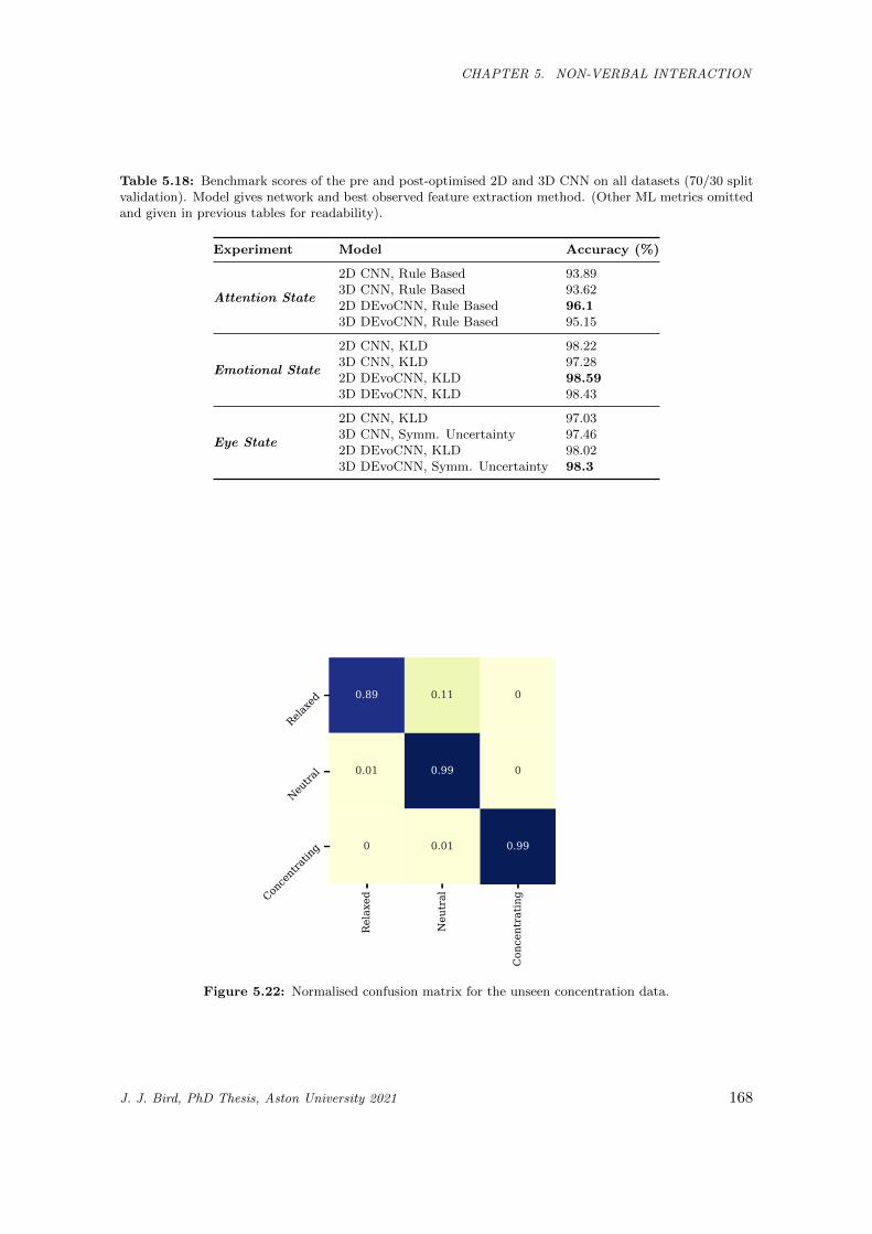
CHAPTER 5. NON-VERBAL INTERACTION
Table 5.18: Benchmark scores of the pre and post-optimised 2D and 3D CNN on all datasets (70/30 splitvalidation). Model gives network and best observed feature extraction method. (Other ML metrics omittedand given in previous tables for readability).
Experiment Model Accuracy (%)
Attention State
2D CNN, Rule Based 93.893D CNN, Rule Based 93.622D DEvoCNN, Rule Based 96.13D DEvoCNN, Rule Based 95.15
Emotional State
2D CNN, KLD 98.223D CNN, KLD 97.282D DEvoCNN, KLD 98.593D DEvoCNN, KLD 98.43
Eye State
2D CNN, KLD 97.033D CNN, Symm. Uncertainty 97.462D DEvoCNN, KLD 98.023D DEvoCNN, Symm. Uncertainty 98.3
Relaxed
Neu
tral
Con
centratin
g
Relaxed
Neutral
Concentrating
0.89 0.11 0
0.01 0.99 0
0 0.01 0.99
Figure 5.22: Normalised confusion matrix for the unseen concentration data.
J. J. Bird, PhD Thesis, Aston University 2021 168
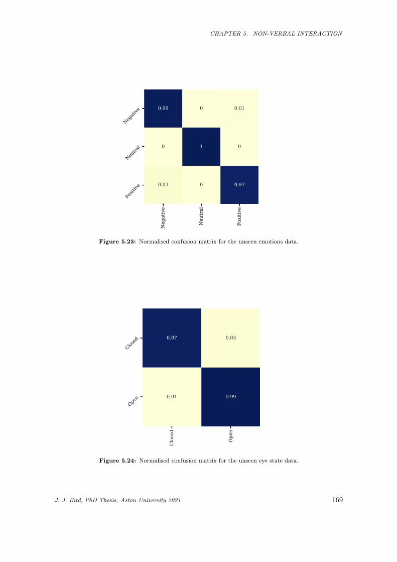
CHAPTER 5. NON-VERBAL INTERACTION
Neg
ative
Neu
tral
Positiv
e
Negative
Neutral
Positive
0.99 0 0.01
0 1 0
0.03 0 0.97
Figure 5.23: Normalised confusion matrix for the unseen emotions data.
Closed
Ope
n
Closed
Open
0.97 0.03
0.01 0.99
Figure 5.24: Normalised confusion matrix for the unseen eye state data.
J. J. Bird, PhD Thesis, Aston University 2021 169
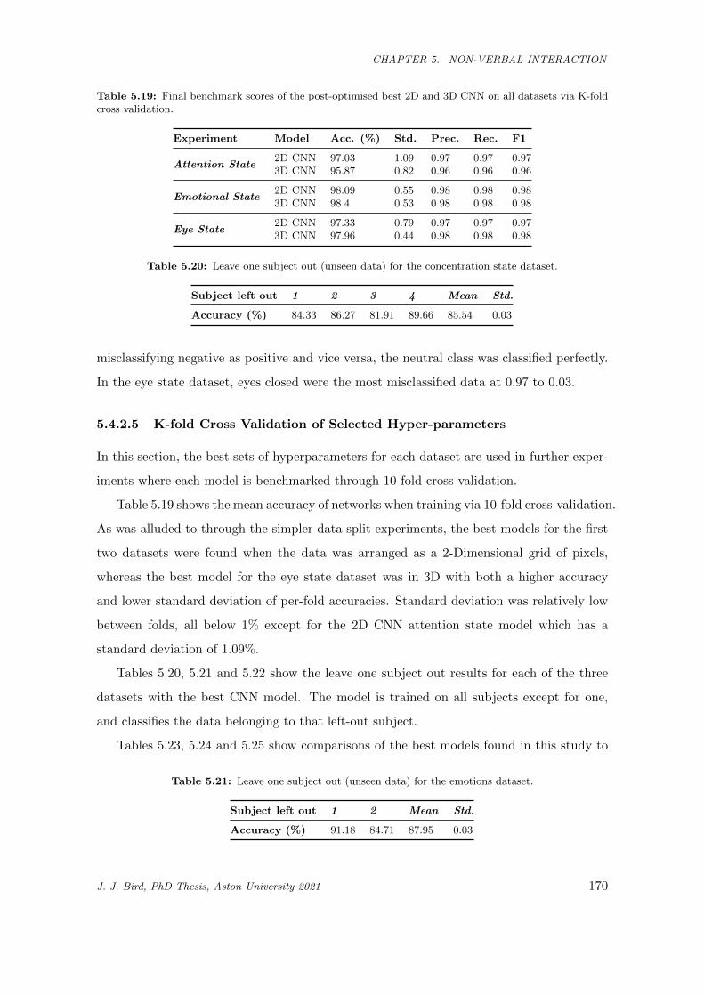
CHAPTER 5. NON-VERBAL INTERACTION
Table 5.19: Final benchmark scores of the post-optimised best 2D and 3D CNN on all datasets via K-foldcross validation.
Experiment Model Acc. (%) Std. Prec. Rec. F1
Attention State2D CNN 97.03 1.09 0.97 0.97 0.973D CNN 95.87 0.82 0.96 0.96 0.96
Emotional State2D CNN 98.09 0.55 0.98 0.98 0.983D CNN 98.4 0.53 0.98 0.98 0.98
Eye State2D CNN 97.33 0.79 0.97 0.97 0.973D CNN 97.96 0.44 0.98 0.98 0.98
Table 5.20: Leave one subject out (unseen data) for the concentration state dataset.
Subject left out 1 2 3 4 Mean Std.
Accuracy (%) 84.33 86.27 81.91 89.66 85.54 0.03
misclassifying negative as positive and vice versa, the neutral class was classified perfectly.
In the eye state dataset, eyes closed were the most misclassified data at 0.97 to 0.03.
5.4.2.5 K-fold Cross Validation of Selected Hyper-parameters
In this section, the best sets of hyperparameters for each dataset are used in further exper-
iments where each model is benchmarked through 10-fold cross-validation.
Table 5.19 shows the mean accuracy of networks when training via 10-fold cross-validation.
As was alluded to through the simpler data split experiments, the best models for the first
two datasets were found when the data was arranged as a 2-Dimensional grid of pixels,
whereas the best model for the eye state dataset was in 3D with both a higher accuracy
and lower standard deviation of per-fold accuracies. Standard deviation was relatively low
between folds, all below 1% except for the 2D CNN attention state model which has a
standard deviation of 1.09%.
Tables 5.20, 5.21 and 5.22 show the leave one subject out results for each of the three
datasets with the best CNN model. The model is trained on all subjects except for one,
and classifies the data belonging to that left-out subject.
Tables 5.23, 5.24 and 5.25 show comparisons of the best models found in this study to
Table 5.21: Leave one subject out (unseen data) for the emotions dataset.
Subject left out 1 2 Mean Std.
Accuracy (%) 91.18 84.71 87.95 0.03
J. J. Bird, PhD Thesis, Aston University 2021 170
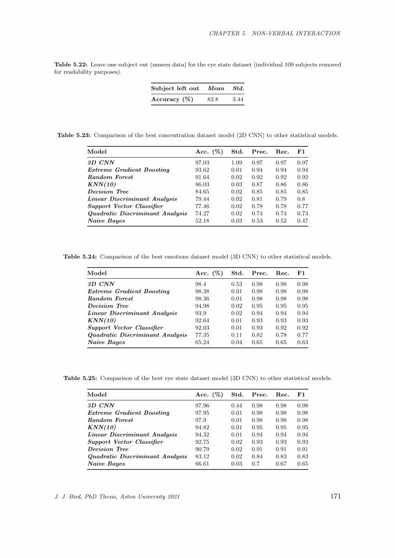
CHAPTER 5. NON-VERBAL INTERACTION
Table 5.22: Leave one subject out (unseen data) for the eye state dataset (individual 109 subjects removedfor readability purposes).
Subject left out Mean Std.
Accuracy (%) 83.8 3.44
Table 5.23: Comparison of the best concentration dataset model (2D CNN) to other statistical models.
Model Acc. (%) Std. Prec. Rec. F1
2D CNN 97.03 1.09 0.97 0.97 0.97Extreme Gradient Boosting 93.62 0.01 0.94 0.94 0.94Random Forest 91.64 0.02 0.92 0.92 0.92KNN(10) 86.03 0.03 0.87 0.86 0.86Decision Tree 84.65 0.02 0.85 0.85 0.85Linear Discriminant Analysis 79.44 0.02 0.81 0.79 0.8Support Vector Classifier 77.46 0.02 0.78 0.78 0.77Quadratic Discriminant Analysis 74.27 0.02 0.74 0.74 0.73Naive Bayes 52.18 0.03 0.53 0.52 0.47
Table 5.24: Comparison of the best emotions dataset model (3D CNN) to other statistical models.
Model Acc. (%) Std. Prec. Rec. F1
3D CNN 98.4 0.53 0.98 0.98 0.98Extreme Gradient Boosting 98.38 0.01 0.98 0.98 0.98Random Forest 98.36 0.01 0.98 0.98 0.98Decision Tree 94.98 0.02 0.95 0.95 0.95Linear Discriminant Analysis 93.9 0.02 0.94 0.94 0.94KNN(10) 92.64 0.01 0.93 0.93 0.93Support Vector Classifier 92.03 0.01 0.93 0.92 0.92Quadratic Discriminant Analysis 77.35 0.11 0.82 0.78 0.77Naive Bayes 65.24 0.04 0.65 0.65 0.63
Table 5.25: Comparison of the best eye state dataset model (3D CNN) to other statistical models.
Model Acc. (%) Std. Prec. Rec. F1
3D CNN 97.96 0.44 0.98 0.98 0.98Extreme Gradient Boosting 97.95 0.01 0.98 0.98 0.98Random Forest 97.9 0.01 0.98 0.98 0.98KNN(10) 94.82 0.01 0.95 0.95 0.95Linear Discriminant Analysis 94.32 0.01 0.94 0.94 0.94Support Vector Classifier 92.75 0.02 0.93 0.93 0.93Decision Tree 90.79 0.02 0.91 0.91 0.91Quadratic Discriminant Analysis 83.12 0.02 0.84 0.83 0.83Naive Bayes 66.61 0.03 0.7 0.67 0.65
J. J. Bird, PhD Thesis, Aston University 2021 171
CHAPTER 5. NON-VERBAL INTERACTION
other statistical machine learning models. Although the top mean scores were noted to be
the CNNs found in this study, their deviance is relatively high. In some cases such as in the
emotions and eye state datasets for example, the CNN only slightly outperforms a Random
Forest, which is far less computationally expensive to execute in comparison. Although the
experiments in this work are chosen because of a small amount of increase in classification
accuracy, the size of the dataset leads to a small increase of accuracy covering the correct
classification of a considerable number of samples.
5.5 Real-time EMG classification via Inductive and Super-
vised Transductive Transfer Learning
Within a social context, the current state of Human-Robot Interaction is arguably most
often concerned with the domain of verbal, spoken communication. That is, the transcrip-
tion of spoken language to text, and further Natural Language Processing (NLP) in order
to extract meaning; this framework is oftentimes multi-modally combined with other data,
such as the tone of voice, which too carries useful information. With this in mind, a recent
National GP Survey carried out in the United Kingdom found that 125,000 adults and
20,000 children had the ability to converse in British Sign Language (BSL) [387], and of
those surveyed, 15,000 people reported it as their primary language. With those statistics
in mind, this shows that those 15,000 people only have the ability to directly converse with
approximately 0.22% of the UK population. This argues for the importance of non-verbal
communication, such as through gesture. To answer in the affirmative, negative, or to not
answer at all are three very important responses when it comes to meaningful conversation,
especially in a goal-based scenario. In this study, a ternary classification experiment is
performed towards the domain of non-verbal communication with robots; the electromyo-
graphic signals produced when performing a thumbs up, thumbs down, and resting state
with either the left or right arms are considered, and statistical classification techniques
are benchmarked in terms of validation, generalisation to new data, and transfer learning
to better generalise to new data to increase reliability within the realms of classical speech
recognition. That is, to reach interchangeable accuracy between the two domains and thus
enable those who do not have the ability of speech to effectively communicate with machines.
The main contributions of this work are as follows:
J. J. Bird, PhD Thesis, Aston University 2021 172
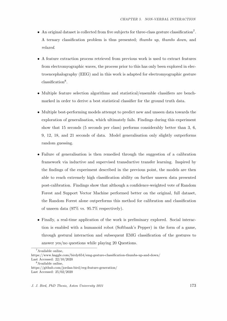
CHAPTER 5. NON-VERBAL INTERACTION
• An original dataset is collected from five subjects for three-class gesture classification7.
A ternary classification problem is thus presented; thumbs up, thumbs down, and
relaxed.
• A feature extraction process retrieved from previous work is used to extract features
from electromyographic waves, the process prior to this has only been explored in elec-
troencephalography (EEG) and in this work is adapted for electromyographic gesture
classification8.
• Multiple feature selection algorithms and statistical/ensemble classifiers are bench-
marked in order to derive a best statistical classifier for the ground truth data.
• Multiple best-performing models attempt to predict new and unseen data towards the
exploration of generalisation, which ultimately fails. Findings during this experiment
show that 15 seconds (5 seconds per class) performs considerably better than 3, 6,
9, 12, 18, and 21 seconds of data. Model generalisation only slightly outperforms
random guessing.
• Failure of generalisation is then remedied through the suggestion of a calibration
framework via inductive and supervised transductive transfer learning. Inspired by
the findings of the experiment described in the previous point, the models are then
able to reach extremely high classification ability on further unseen data presented
post-calibration. Findings show that although a confidence-weighted vote of Random
Forest and Support Vector Machine performed better on the original, full dataset,
the Random Forest alone outperforms this method for calibration and classification
of unseen data (97% vs. 95.7% respectively).
• Finally, a real-time application of the work is preliminary explored. Social interac-
tion is enabled with a humanoid robot (Softbank’s Pepper) in the form of a game,
through gestural interaction and subsequent EMG classification of the gestures to
answer yes/no questions while playing 20 Questions.
7Available online,https://www.kaggle.com/birdy654/emg-gesture-classification-thumbs-up-and-down/Last Accessed: 22/10/2020
8Available online,https://github.com/jordan-bird/eeg-feature-generation/Last Accessed: 25/02/2020
J. J. Bird, PhD Thesis, Aston University 2021 173
CHAPTER 5. NON-VERBAL INTERACTION
To present the aforementioned findings in a structured manner, the exploration and
results are presented in chronological order, since a failed generalisation experiment is then
remedied with the aid of the findings through limitation.
5.5.1 Method
In this section, the methodology of the experiments in this study are described. Initially,
data is acquired prior to the generation of a full dataset through feature extraction. Machine
Learning paradigms are then benchmarked on the dataset, before the exploration of real-
time classification of unseen data.
The experiments performed in this study were executed on a AMD FX-8520 eight-core
processor with a clock speed of 3.8GHz. In terms of software, the algorithms are executed
via the Weka API (implemented in Java). The machine learning algorithms are validated
through a process of k-fold cross validation, where k is set to 10 folds. The voting process
is to vote by average probabilities of the models, since two models are considered and
thus a democratic voting process would result in a tie should the two models disagree.
Machine learning is employed towards solving this problem of gesture classification since
accelerometer and gyroscope sensors are not used, and thus the classification of only EMG
data proves a difficult problem.
The Myo Armband records EMG data at a rate of 200Hz via 8 dry sensors worn on
the arm, and it also has a 9-axis Inertial Measurement Unit (IMU) recording at a sample
rate of 50Hz. Further details on the Myo can be found in Section 5.2.2. In this study, data
acquisition is performed on 5 subjects, which are three males and two females (aged 22-40).
For model generalisation, 4 more subjects ware taken into account, of which two of them
are new subjects and two are performing the movements again. The gestures performed
were thumbs up, thumbs down, and resting (a neutral gesture in which the subject is asked
to rest their hand). For training, 60 seconds of forearm muscle activity data was recorded
for each arm (two minutes, per subject, per gesture). In the case of benchmark data, the
muscle waves were recorded in intervals of one to seven seconds each.
As previously described in Section 5.2.3, features are then extracted from the waves via
a sliding time window statistic extraction algorithm. Feature extraction thus produced a
dataset of 2040 numerical attributes from the 8 electrodes, of which there are 159 megabytes
of data produced from the five subjects. A minor original contribution is also presented in
J. J. Bird, PhD Thesis, Aston University 2021 174
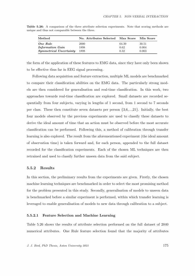
CHAPTER 5. NON-VERBAL INTERACTION
Table 5.26: A comparison of the three attribute selection experiments. Note that scoring methods areunique and thus not comparable between the three.
Method No. Attributes Selected Max Score Min Score
One Rule 2000 64.39 30.51Information Gain 1898 0.62 0.004Symmetrical Uncertainty 1898 0.32 0.003
the form of the application of these features to EMG data, since they have only been shown
to be effective thus far in EEG signal processing.
Following data acquisition and feature extraction, multiple ML models are benchmarked
to compare their classification abilities on the EMG data. The particularly strong mod-
els are then considered for generalisation and real-time classification. In this work, two
approaches towards real-time classification are explored. Small datasets are recorded se-
quentially from four subjects, varying in lengths of 1 second, from 1 second to 7 seconds
per class. These then constitute seven datasets per person {3,6,...,21}. Initially, the best
four models observed by the previous experiments are used to classify these datasets to
derive the ideal amount of time that an action must be observed before the most accurate
classification can be performed. Following this, a method of calibration through transfer
learning is also explored. The result from the aforementioned experiment (the ideal amount
of observation time) is taken forward and, for each person, appended to the full dataset
recorded for the classification experiments. Each of the chosen ML techniques are then
retrained and used to classify further unseen data from the said subject.
5.5.2 Results
In this section, the preliminary results from the experiments are given. Firstly, the chosen
machine learning techniques are benchmarked in order to select the most promising method
for the problem presented in this study. Secondly, generalisation of models to unseen data
is benchmarked before a similar experiment is performed, within which transfer learning is
leveraged to enable generalisation of models to new data through calibration to a subject.
5.5.2.1 Feature Selection and Machine Learning
Table 5.26 shows the results of attribute selection performed on the full dataset of 2040
numerical attributes. One Rule feature selection found that the majority of attributes
J. J. Bird, PhD Thesis, Aston University 2021 175

CHAPTER 5. NON-VERBAL INTERACTION
held strong One Rule classification ability, as is often expected [388]. Information Gain and
Symmetrical Uncertainty produced slightly smaller datasets, both of 1898 rows, and it must
be noted that the two datasets are comprised of differing attributes.
J. J. Bird, PhD Thesis, Aston University 2021 176
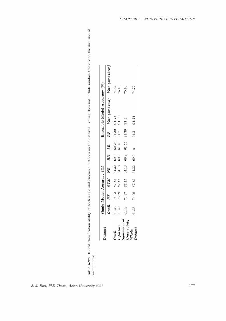
CHAPTER 5. NON-VERBAL INTERACTION
Table
5.27:
10-f
old
class
ifica
tion
ab
ilit
yof
both
sin
gle
an
den
sem
ble
met
hod
son
the
data
sets
.V
oti
ng
does
not
incl
ud
era
nd
om
tree
du
eto
the
incl
usi
on
of
ran
dom
fore
st.
Data
set
Single
ModelAccura
cy
(%)
Ense
mble
ModelAccura
cy
(%)
OneR
RT
SVM
NB
BN
LR
RF
Vote
(best
two)
Vote
(best
three)
OneR
61.3
374.0
387.14
64.3
269.9
60.7
691.3
091.74
74.6
7In
foGain
61.4
975.3
987.11
64.1
369.9
61.4
591.7
91.30
75.1
3Symmetrical
Unce
rtain
ty61.4
874.3
787.11
64.1
369.9
61.5
591.3
691.4
75.1
6
Whole
Datase
t61.3
374.0
987.14
64.3
269.9
x91.3
91.71
74.7
2
J. J. Bird, PhD Thesis, Aston University 2021 177
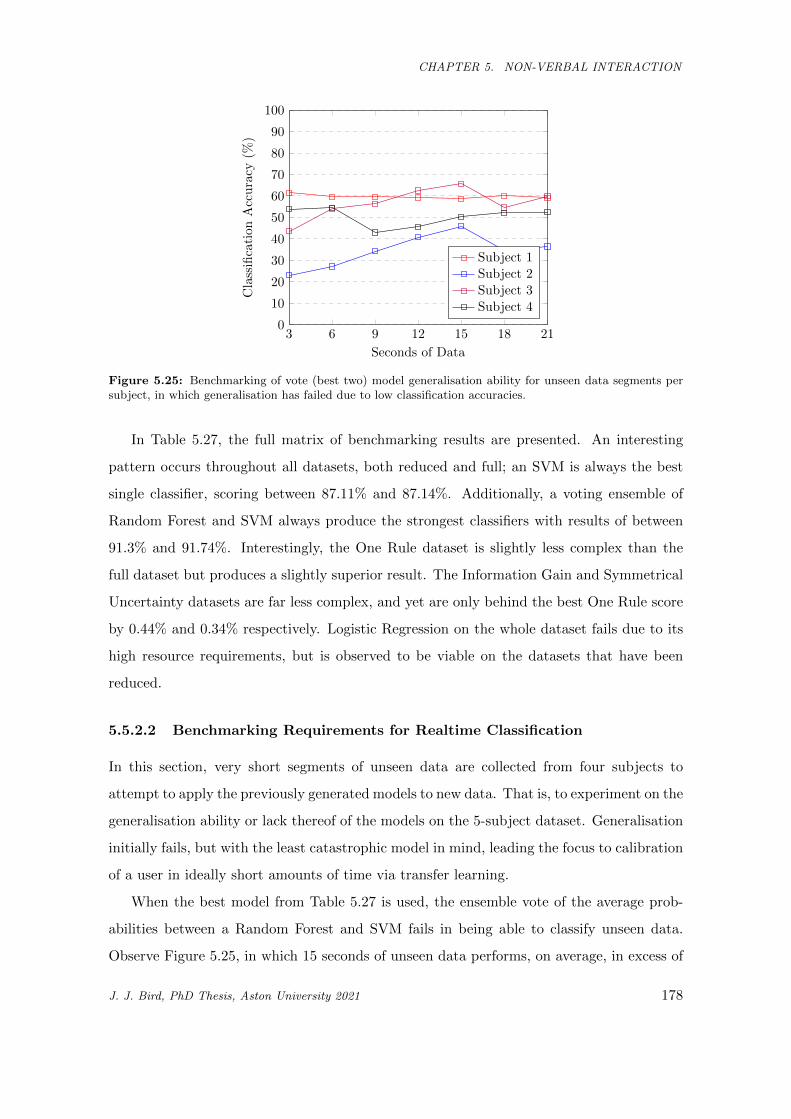
CHAPTER 5. NON-VERBAL INTERACTION
3 6 9 12 15 18 210
10
20
30
40
50
60
70
80
90
100
Seconds of Data
Cla
ssifi
cati
onA
ccu
racy
(%)
Subject 1Subject 2Subject 3Subject 4
Figure 5.25: Benchmarking of vote (best two) model generalisation ability for unseen data segments persubject, in which generalisation has failed due to low classification accuracies.
In Table 5.27, the full matrix of benchmarking results are presented. An interesting
pattern occurs throughout all datasets, both reduced and full; an SVM is always the best
single classifier, scoring between 87.11% and 87.14%. Additionally, a voting ensemble of
Random Forest and SVM always produce the strongest classifiers with results of between
91.3% and 91.74%. Interestingly, the One Rule dataset is slightly less complex than the
full dataset but produces a slightly superior result. The Information Gain and Symmetrical
Uncertainty datasets are far less complex, and yet are only behind the best One Rule score
by 0.44% and 0.34% respectively. Logistic Regression on the whole dataset fails due to its
high resource requirements, but is observed to be viable on the datasets that have been
reduced.
5.5.2.2 Benchmarking Requirements for Realtime Classification
In this section, very short segments of unseen data are collected from four subjects to
attempt to apply the previously generated models to new data. That is, to experiment on the
generalisation ability or lack thereof of the models on the 5-subject dataset. Generalisation
initially fails, but with the least catastrophic model in mind, leading the focus to calibration
of a user in ideally short amounts of time via transfer learning.
When the best model from Table 5.27 is used, the ensemble vote of the average prob-
abilities between a Random Forest and SVM fails in being able to classify unseen data.
Observe Figure 5.25, in which 15 seconds of unseen data performs, on average, in excess of
J. J. Bird, PhD Thesis, Aston University 2021 178
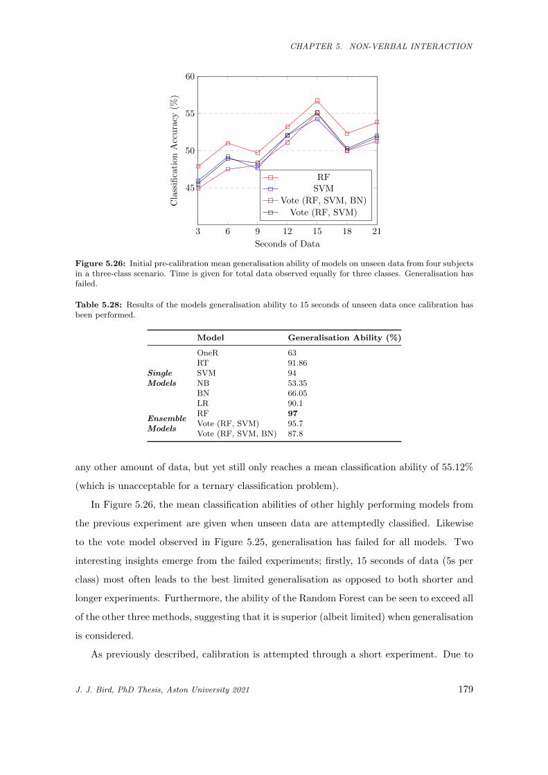
CHAPTER 5. NON-VERBAL INTERACTION
3 6 9 12 15 18 21
45
50
55
60
Seconds of Data
Cla
ssifi
cati
onA
ccu
racy
(%)
RFSVM
Vote (RF, SVM, BN)
Vote (RF, SVM)
Figure 5.26: Initial pre-calibration mean generalisation ability of models on unseen data from four subjectsin a three-class scenario. Time is given for total data observed equally for three classes. Generalisation hasfailed.
Table 5.28: Results of the models generalisation ability to 15 seconds of unseen data once calibration hasbeen performed.
Model Generalisation Ability (%)
SingleModels
OneR 63RT 91.86SVM 94NB 53.35BN 66.05LR 90.1
EnsembleModels
RF 97Vote (RF, SVM) 95.7Vote (RF, SVM, BN) 87.8
any other amount of data, but yet still only reaches a mean classification ability of 55.12%
(which is unacceptable for a ternary classification problem).
In Figure 5.26, the mean classification abilities of other highly performing models from
the previous experiment are given when unseen data are attemptedly classified. Likewise
to the vote model observed in Figure 5.25, generalisation has failed for all models. Two
interesting insights emerge from the failed experiments; firstly, 15 seconds of data (5s per
class) most often leads to the best limited generalisation as opposed to both shorter and
longer experiments. Furthermore, the ability of the Random Forest can be seen to exceed all
of the other three methods, suggesting that it is superior (albeit limited) when generalisation
is considered.
As previously described, calibration is attempted through a short experiment. Due to
J. J. Bird, PhD Thesis, Aston University 2021 179
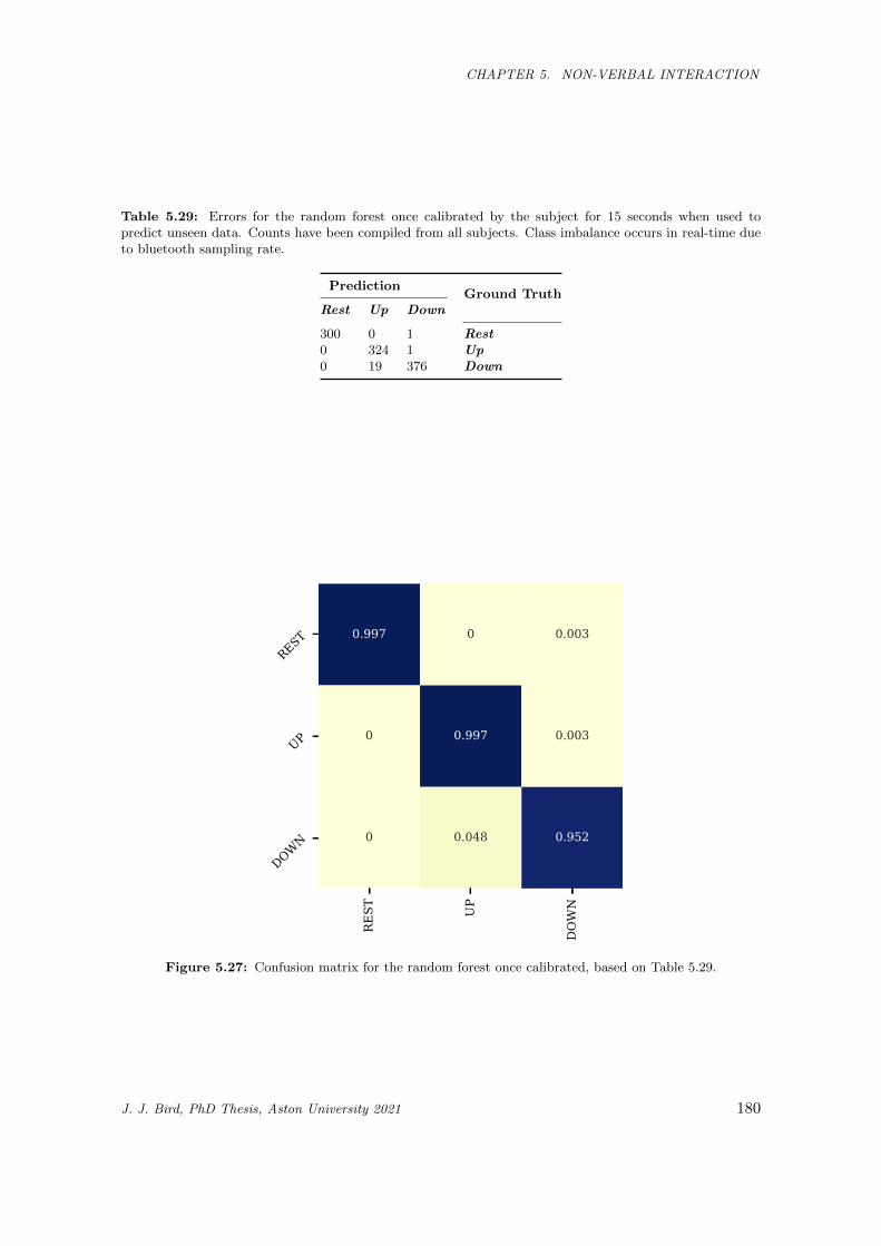
CHAPTER 5. NON-VERBAL INTERACTION
Table 5.29: Errors for the random forest once calibrated by the subject for 15 seconds when used topredict unseen data. Counts have been compiled from all subjects. Class imbalance occurs in real-time dueto bluetooth sampling rate.
PredictionGround Truth
Rest Up Down
300 0 1 Rest0 324 1 Up0 19 376 Down
REST UP
DOWN
REST
UP
DOWN
0.997 0 0.003
0 0.997 0.003
0 0.048 0.952
Figure 5.27: Confusion matrix for the random forest once calibrated, based on Table 5.29.
J. J. Bird, PhD Thesis, Aston University 2021 180
CHAPTER 5. NON-VERBAL INTERACTION
the findings aforementioned, 15 seconds of known data (that is, requested during ‘setup’ )
is collected. These labelled data are then added to the training data, to expand knowledge
at a personal level. Once this is performed, and the models are trained, they are then
benchmarked on a further unseen dataset of 15 seconds of data, again, five seconds per
class. No further training of models are performed, and they simply attempt to classify this
unseen data. Table 5.28 shows the abilities of all previously benchmarked models once the
short calibration process is followed, with far greater success than observed in the previous
failed experiments, where those previous were benchmarked. As was conjectured from
the failed experiments, the Random Forest showed to be the most successful calibration
experiment for generalisation towards a new subject. The errors made by the best model
are shown in in Table 5.29 and Figure 5.27. The most difficult task was the prediction of
‘thumbs down’, which, when a subject had a particularly smaller arm would sometimes be
classified as a resting state. Observed errors are extremely low, and thus future work to
explore this is suggested in Section 5.8.
Following the results, an application of the framework is presented in a HRI context. The
Random Forest model observed to be the best model for generalisation in Section 5.5.2.2
is calibrated for 5 seconds per class in regards to the benchmark results, then enabling the
subject to interact non-verbally with machines via EMG gesture classification. Note that
only preliminary benchmarks are presented, and Section 5.8 details potential future works
in this regard, that is, these preliminary activities are not considered the main contributions
of this work which were presented in Section 5.5.2.
20Q, or 20 Questions, is a digital game developed by Robin Burgener based on the
20th Century American parlor game of the same name and rules; it is a situational puzzle.
Through Burgener’s algorithm, computer opponents play via the dissemination and subse-
quent strategy presented by an Artificial Neural Network [389, 390]. In the game between
man and machine, the player thinks of an entity and the opponent is able to ask 20 yes/no
questions. Through elimination of potential answers, the opponent is free to guess the entity
that the player is thinking of. If the opponent cannot guess the entity by the end of the 20
questions, then the player has won.
In this application, the 20 Questions game is played with a humanoid robot, Softbank
Robotics’ Pepper. Initially, the subject is calibrated with 15 seconds of data (5 per class)
added to the full dataset, due to the findings in this work. Following this, for every round
J. J. Bird, PhD Thesis, Aston University 2021 181
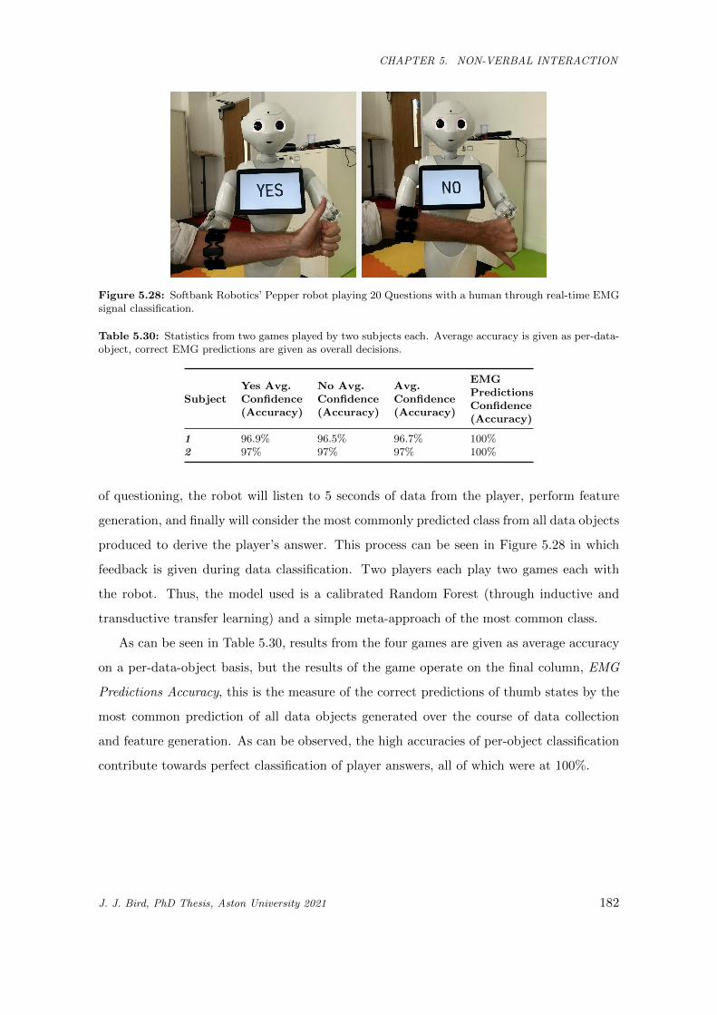
CHAPTER 5. NON-VERBAL INTERACTION
Figure 5.28: Softbank Robotics’ Pepper robot playing 20 Questions with a human through real-time EMGsignal classification.
Table 5.30: Statistics from two games played by two subjects each. Average accuracy is given as per-data-object, correct EMG predictions are given as overall decisions.
SubjectYes Avg.Confidence(Accuracy)
No Avg.Confidence(Accuracy)
Avg.Confidence(Accuracy)
EMGPredictionsConfidence(Accuracy)
1 96.9% 96.5% 96.7% 100%2 97% 97% 97% 100%
of questioning, the robot will listen to 5 seconds of data from the player, perform feature
generation, and finally will consider the most commonly predicted class from all data objects
produced to derive the player’s answer. This process can be seen in Figure 5.28 in which
feedback is given during data classification. Two players each play two games each with
the robot. Thus, the model used is a calibrated Random Forest (through inductive and
transductive transfer learning) and a simple meta-approach of the most common class.
As can be seen in Table 5.30, results from the four games are given as average accuracy
on a per-data-object basis, but the results of the game operate on the final column, EMG
Predictions Accuracy, this is the measure of the correct predictions of thumb states by the
most common prediction of all data objects generated over the course of data collection
and feature generation. As can be observed, the high accuracies of per-object classification
contribute towards perfect classification of player answers, all of which were at 100%.
J. J. Bird, PhD Thesis, Aston University 2021 182
CHAPTER 5. NON-VERBAL INTERACTION
5.6 Data Augmentation by Synthetic Biological Signals Machine-
generated by GPT-2
Given that it was discovered in Section 4.3 that speaker recognition could be improved when
GPT-2 creates synthetic training data to augment the training process, this section explores
the application of a similar Transformer based approach for the improvement of biological
signal classification. Synthetic data augmentation is of paramount importance for machine
learning classification, particularly for biological data, which tend to be high dimensional
and with a scarcity of training samples, moreover, they can rarely be generalised to the
whole population and appear to over-complicate simple recognition tasks. This work shows
for the first time that multiple GPT-2 models can machine-generate synthetic EEG signals
and improve real classification processes.
When presenting their GPT model, researchers at OpenAI hypothesised that language
models are unsupervised multitask learners [391, 392]. At the current state-of-the-art, this
claim has been proven correct multiple times through applications such as fake news iden-
tification [393], patent claims [394], and stock market analysis [395] to name just a few
in a rapidly growing area of research. In this work, experiments follow those before who
explored the capabilities of these models in a brand new field of application: the generation
of biosynthetic signals (in this case, electroencephalographic (EEG) activity). In detail,
this work aimed at exploring whether or not GPT-2’s self-attention based architecture was
capable of creating synthetic signals, and if those signals could improve the performance of
classification models used on real datasets. The scientific contributions and results arising
from this work suggest that:
1. It is possible to generate synthetic biological signals by tuning a language transfor-
mation model.
2. Classifiers trained on either real or synthetic data can classify one another with rela-
tively high accuracy.
3. Synthetic data improves the classification of the real data both in terms of model
benchmarking and classification of unseen samples.
J. J. Bird, PhD Thesis, Aston University 2021 183
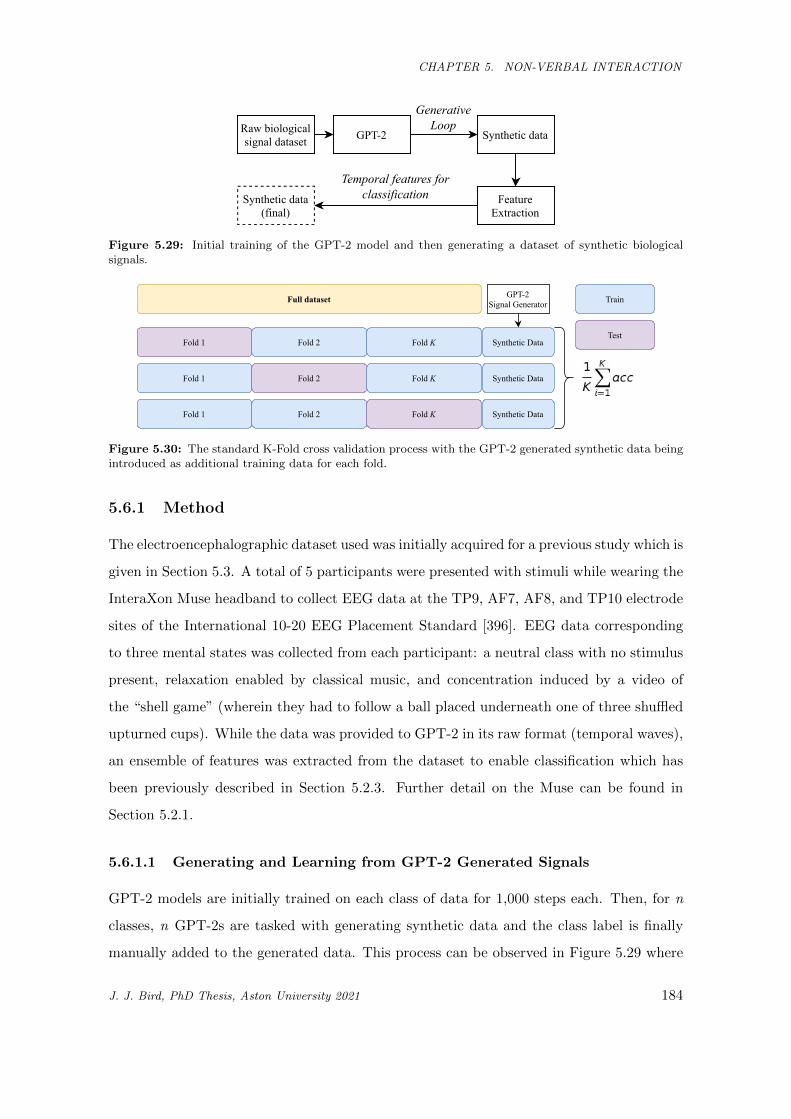
CHAPTER 5. NON-VERBAL INTERACTION
Rawbiologicalsignaldataset GPT-2 Syntheticdata
GenerativeLoop
Syntheticdata(final)
Temporalfeaturesforclassification Feature
Extraction
Figure 5.29: Initial training of the GPT-2 model and then generating a dataset of synthetic biologicalsignals.
Fold1 Fold2 FoldK
Fulldataset
SyntheticData
GPT-2SignalGenerator
Fold1 Fold2 FoldK SyntheticData
Fold1 Fold2 FoldK SyntheticData
Train
Test
Figure 5.30: The standard K-Fold cross validation process with the GPT-2 generated synthetic data beingintroduced as additional training data for each fold.
5.6.1 Method
The electroencephalographic dataset used was initially acquired for a previous study which is
given in Section 5.3. A total of 5 participants were presented with stimuli while wearing the
InteraXon Muse headband to collect EEG data at the TP9, AF7, AF8, and TP10 electrode
sites of the International 10-20 EEG Placement Standard [396]. EEG data corresponding
to three mental states was collected from each participant: a neutral class with no stimulus
present, relaxation enabled by classical music, and concentration induced by a video of
the “shell game” (wherein they had to follow a ball placed underneath one of three shuffled
upturned cups). While the data was provided to GPT-2 in its raw format (temporal waves),
an ensemble of features was extracted from the dataset to enable classification which has
been previously described in Section 5.2.3. Further detail on the Muse can be found in
Section 5.2.1.
5.6.1.1 Generating and Learning from GPT-2 Generated Signals
GPT-2 models are initially trained on each class of data for 1,000 steps each. Then, for n
classes, n GPT-2s are tasked with generating synthetic data and the class label is finally
manually added to the generated data. This process can be observed in Figure 5.29 where
J. J. Bird, PhD Thesis, Aston University 2021 184
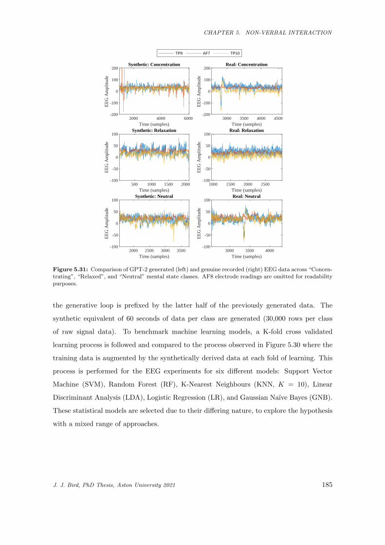
CHAPTER 5. NON-VERBAL INTERACTION
2000 4000 6000Time (samples)
-200
-100
0
100
200
EE
G A
mpl
itude
Synthetic: Concentration
3000 3500 4000 4500Time (samples)
-200
-100
0
100
200
EE
G A
mpl
itude
Real: Concentration
500 1000 1500 2000Time (samples)
-100
-50
0
50
100
EE
G A
mpl
itude
Synthetic: Relaxation
1000 1500 2000 2500Time (samples)
-100
-50
0
50
100
EE
G A
mpl
itude
Real: Relaxation
2000 2500 3000 3500Time (samples)
-100
-50
0
50
100
EE
G A
mpl
itude
Synthetic: Neutral
3000 3500 4000Time (samples)
-100
-50
0
50
100E
EG
Am
plitu
deReal: Neutral
TP9 AF7 TP10
Figure 5.31: Comparison of GPT-2 generated (left) and genuine recorded (right) EEG data across “Concen-trating”, “Relaxed”, and “Neutral” mental state classes. AF8 electrode readings are omitted for readabilitypurposes.
the generative loop is prefixed by the latter half of the previously generated data. The
synthetic equivalent of 60 seconds of data per class are generated (30,000 rows per class
of raw signal data). To benchmark machine learning models, a K-fold cross validated
learning process is followed and compared to the process observed in Figure 5.30 where the
training data is augmented by the synthetically derived data at each fold of learning. This
process is performed for the EEG experiments for six different models: Support Vector
Machine (SVM), Random Forest (RF), K-Nearest Neighbours (KNN, K = 10), Linear
Discriminant Analysis (LDA), Logistic Regression (LR), and Gaussian Naıve Bayes (GNB).
These statistical models are selected due to their differing nature, to explore the hypothesis
with a mixed range of approaches.
J. J. Bird, PhD Thesis, Aston University 2021 185
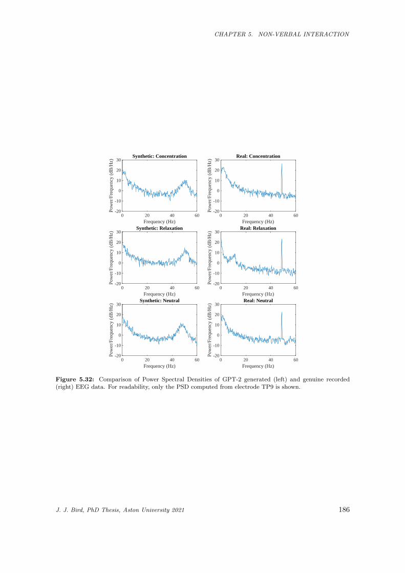
CHAPTER 5. NON-VERBAL INTERACTION
0 20 40 60Frequency (Hz)
-20
-10
0
10
20
30
Pow
er/F
requ
ency
(dB
/Hz)
Synthetic: Concentration
0 20 40 60Frequency (Hz)
-20
-10
0
10
20
30
Pow
er/F
requ
ency
(dB
/Hz)
Real: Concentration
0 20 40 60Frequency (Hz)
-20
-10
0
10
20
30
Pow
er/F
requ
ency
(dB
/Hz)
Synthetic: Relaxation
0 20 40 60Frequency (Hz)
-20
-10
0
10
20
30
Pow
er/F
requ
ency
(dB
/Hz)
Real: Relaxation
0 20 40 60Frequency (Hz)
-20
-10
0
10
20
30
Pow
er/F
requ
ency
(dB
/Hz)
Synthetic: Neutral
0 20 40 60Frequency (Hz)
-20
-10
0
10
20
30
Pow
er/F
requ
ency
(dB
/Hz)
Real: Neutral
Figure 5.32: Comparison of Power Spectral Densities of GPT-2 generated (left) and genuine recorded(right) EEG data. For readability, only the PSD computed from electrode TP9 is shown.
J. J. Bird, PhD Thesis, Aston University 2021 186
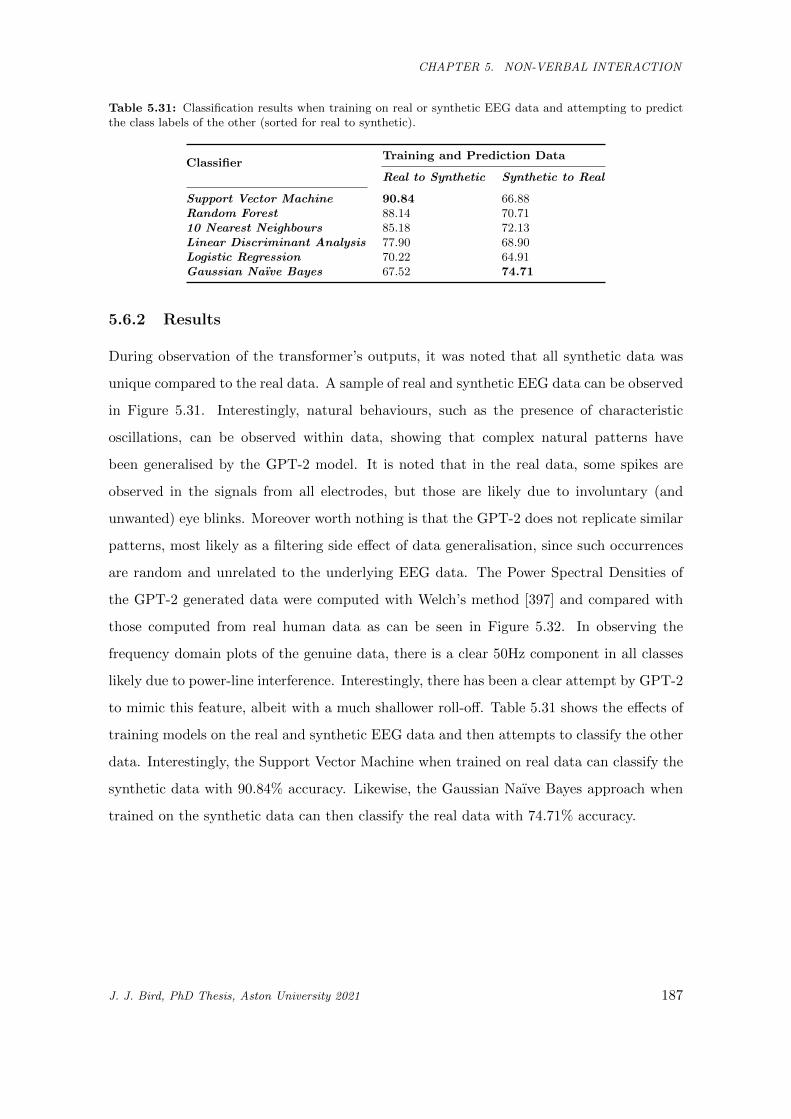
CHAPTER 5. NON-VERBAL INTERACTION
Table 5.31: Classification results when training on real or synthetic EEG data and attempting to predictthe class labels of the other (sorted for real to synthetic).
ClassifierTraining and Prediction Data
Real to Synthetic Synthetic to Real
Support Vector Machine 90.84 66.88Random Forest 88.14 70.7110 Nearest Neighbours 85.18 72.13Linear Discriminant Analysis 77.90 68.90Logistic Regression 70.22 64.91Gaussian Naıve Bayes 67.52 74.71
5.6.2 Results
During observation of the transformer’s outputs, it was noted that all synthetic data was
unique compared to the real data. A sample of real and synthetic EEG data can be observed
in Figure 5.31. Interestingly, natural behaviours, such as the presence of characteristic
oscillations, can be observed within data, showing that complex natural patterns have
been generalised by the GPT-2 model. It is noted that in the real data, some spikes are
observed in the signals from all electrodes, but those are likely due to involuntary (and
unwanted) eye blinks. Moreover worth nothing is that the GPT-2 does not replicate similar
patterns, most likely as a filtering side effect of data generalisation, since such occurrences
are random and unrelated to the underlying EEG data. The Power Spectral Densities of
the GPT-2 generated data were computed with Welch’s method [397] and compared with
those computed from real human data as can be seen in Figure 5.32. In observing the
frequency domain plots of the genuine data, there is a clear 50Hz component in all classes
likely due to power-line interference. Interestingly, there has been a clear attempt by GPT-2
to mimic this feature, albeit with a much shallower roll-off. Table 5.31 shows the effects of
training models on the real and synthetic EEG data and then attempts to classify the other
data. Interestingly, the Support Vector Machine when trained on real data can classify the
synthetic data with 90.84% accuracy. Likewise, the Gaussian Naıve Bayes approach when
trained on the synthetic data can then classify the real data with 74.71% accuracy.
J. J. Bird, PhD Thesis, Aston University 2021 187
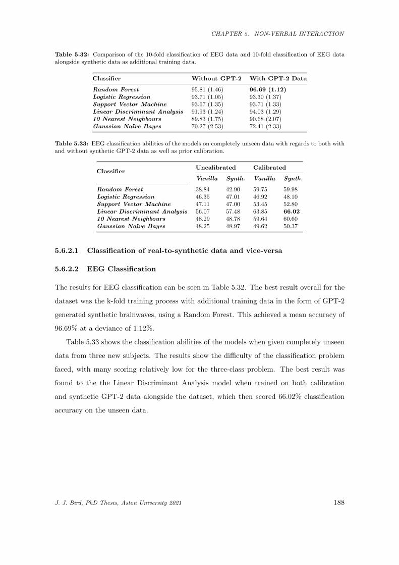
CHAPTER 5. NON-VERBAL INTERACTION
Table 5.32: Comparison of the 10-fold classification of EEG data and 10-fold classification of EEG dataalongside synthetic data as additional training data.
Classifier Without GPT-2 With GPT-2 Data
Random Forest 95.81 (1.46) 96.69 (1.12)Logistic Regression 93.71 (1.05) 93.30 (1.37)Support Vector Machine 93.67 (1.35) 93.71 (1.33)Linear Discriminant Analysis 91.93 (1.24) 94.03 (1.29)10 Nearest Neighbours 89.83 (1.75) 90.68 (2.07)Gaussian Naıve Bayes 70.27 (2.53) 72.41 (2.33)
Table 5.33: EEG classification abilities of the models on completely unseen data with regards to both withand without synthetic GPT-2 data as well as prior calibration.
ClassifierUncalibrated Calibrated
Vanilla Synth. Vanilla Synth.
Random Forest 38.84 42.90 59.75 59.98Logistic Regression 46.35 47.01 46.92 48.10Support Vector Machine 47.11 47.00 53.45 52.80Linear Discriminant Analysis 56.07 57.48 63.85 66.0210 Nearest Neighbours 48.29 48.78 59.64 60.60Gaussian Naıve Bayes 48.25 48.97 49.62 50.37
5.6.2.1 Classification of real-to-synthetic data and vice-versa
5.6.2.2 EEG Classification
The results for EEG classification can be seen in Table 5.32. The best result overall for the
dataset was the k-fold training process with additional training data in the form of GPT-2
generated synthetic brainwaves, using a Random Forest. This achieved a mean accuracy of
96.69% at a deviance of 1.12%.
Table 5.33 shows the classification abilities of the models when given completely unseen
data from three new subjects. The results show the difficulty of the classification problem
faced, with many scoring relatively low for the three-class problem. The best result was
found to the the Linear Discriminant Analysis model when trained on both calibration
and synthetic GPT-2 data alongside the dataset, which then scored 66.02% classification
accuracy on the unseen data.
J. J. Bird, PhD Thesis, Aston University 2021 188
CHAPTER 5. NON-VERBAL INTERACTION
5.7 Cross-Domain MLP and CNN Transfer Learning for Bi-
ological Signal Processing
This section explores the success of unsupervised transfer learning between Electroen-
cephalographic (brainwave) classification and Electromyographic (muscular wave) domains
with both MLP and CNN methods. The significance of this work is due to the success-
ful transfer of ability between models trained on two different biological signal domains,
reducing the need for building more computationally complex models in future research.
It is no secret that the hardware requirements of Deep Learning are far outgrowing the
average consumer level of resource availability, even when a distributed processing device
such as a GPU is considered [398]. In addition to this, limited data availability often ham-
pers the machine learning process. It is for these reasons that researchers often find similar
domains to transfer the learning between, effectively saving computational resources through
said similarities by applying cross-domain interpretation. By doing so, once impossible tasks
become possible, despite limited resources. A well-known example is VGG (Visual Geome-
try Group), a set of 16 and 19 hidden-layer Convolutional Neural Networks (CNNs) which
have been trained to the extreme on a large image dataset [101]. Useful recognisable fea-
tures from images such as points, lines, curves, and geometric shapes can be transferred
over to a differing CNN task since these features always exist within the domain. Thus,
cross-domain transfer learning is enabled in order to interpret new data [399, 400]. Elec-
trical biological signals show a similarly non-juxtapose pattern of behaviour [401, 402], and
thus the domain-transfer may be possible, although it is currently not yet well-understood.
If it is possible, then to what extent and effects are those possibilities?
This work studies, for the first time, whether cross-domain transfer learning can impact
the classification ability of models when trained on Electroencephalographic (brainwave)
and Electromyographic (muscular wave) data. This is performed through the transfer of
initial weights via the best models of each, and learning is continued from this initial starting
point. When compared to the classical method of random weight distribution initialisation,
it is argued that knowledge can be transferred from EMG to EEG and vice-versa, succesfully.
There is also a comparison of the results to a model fine-tuned by ImageNet weights in order
to discern that useful domain-related knowledge is actually being transferred rather than
simply general image rules, which could be learnt from any range of sources and domains.
J. J. Bird, PhD Thesis, Aston University 2021 189
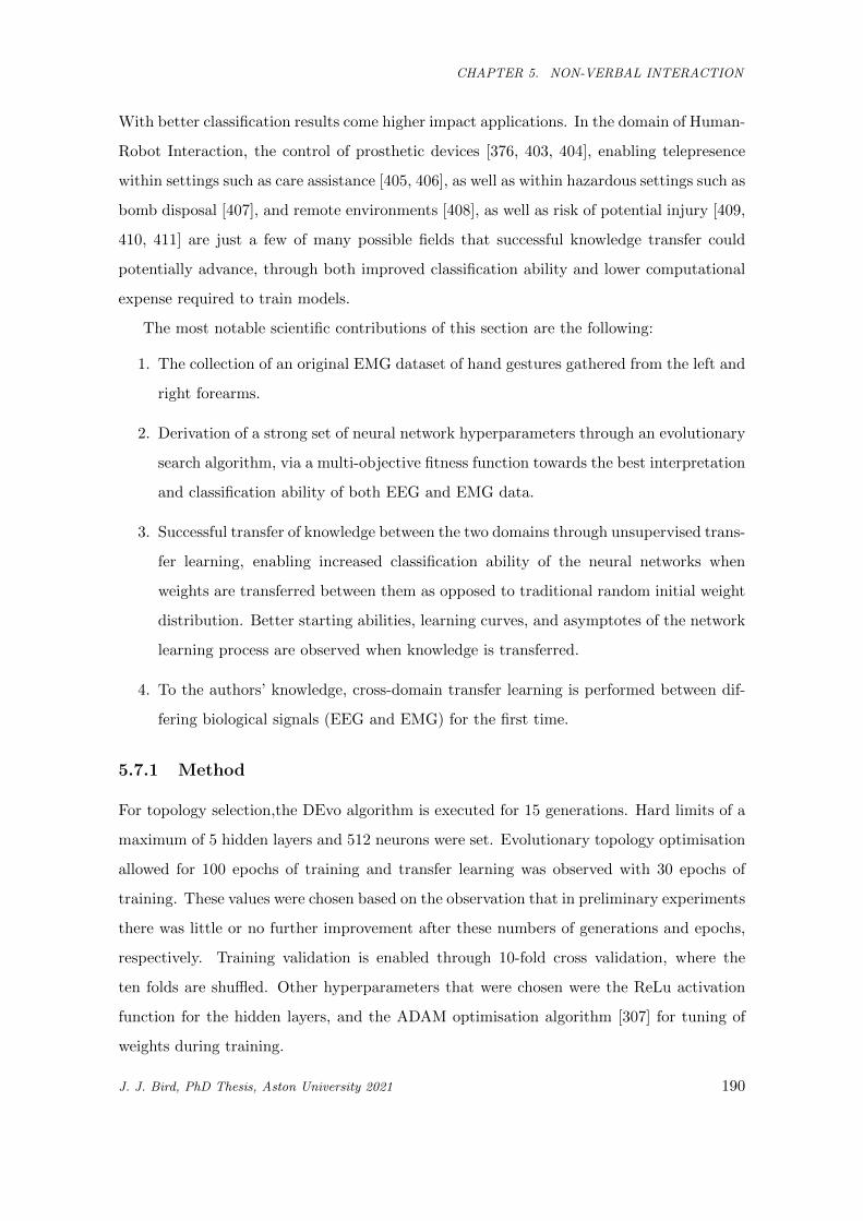
CHAPTER 5. NON-VERBAL INTERACTION
With better classification results come higher impact applications. In the domain of Human-
Robot Interaction, the control of prosthetic devices [376, 403, 404], enabling telepresence
within settings such as care assistance [405, 406], as well as within hazardous settings such as
bomb disposal [407], and remote environments [408], as well as risk of potential injury [409,
410, 411] are just a few of many possible fields that successful knowledge transfer could
potentially advance, through both improved classification ability and lower computational
expense required to train models.
The most notable scientific contributions of this section are the following:
1. The collection of an original EMG dataset of hand gestures gathered from the left and
right forearms.
2. Derivation of a strong set of neural network hyperparameters through an evolutionary
search algorithm, via a multi-objective fitness function towards the best interpretation
and classification ability of both EEG and EMG data.
3. Successful transfer of knowledge between the two domains through unsupervised trans-
fer learning, enabling increased classification ability of the neural networks when
weights are transferred between them as opposed to traditional random initial weight
distribution. Better starting abilities, learning curves, and asymptotes of the network
learning process are observed when knowledge is transferred.
4. To the authors’ knowledge, cross-domain transfer learning is performed between dif-
fering biological signals (EEG and EMG) for the first time.
5.7.1 Method
For topology selection,the DEvo algorithm is executed for 15 generations. Hard limits of a
maximum of 5 hidden layers and 512 neurons were set. Evolutionary topology optimisation
allowed for 100 epochs of training and transfer learning was observed with 30 epochs of
training. These values were chosen based on the observation that in preliminary experiments
there was little or no further improvement after these numbers of generations and epochs,
respectively. Training validation is enabled through 10-fold cross validation, where the
ten folds are shuffled. Other hyperparameters that were chosen were the ReLu activation
function for the hidden layers, and the ADAM optimisation algorithm [307] for tuning of
weights during training.
J. J. Bird, PhD Thesis, Aston University 2021 190
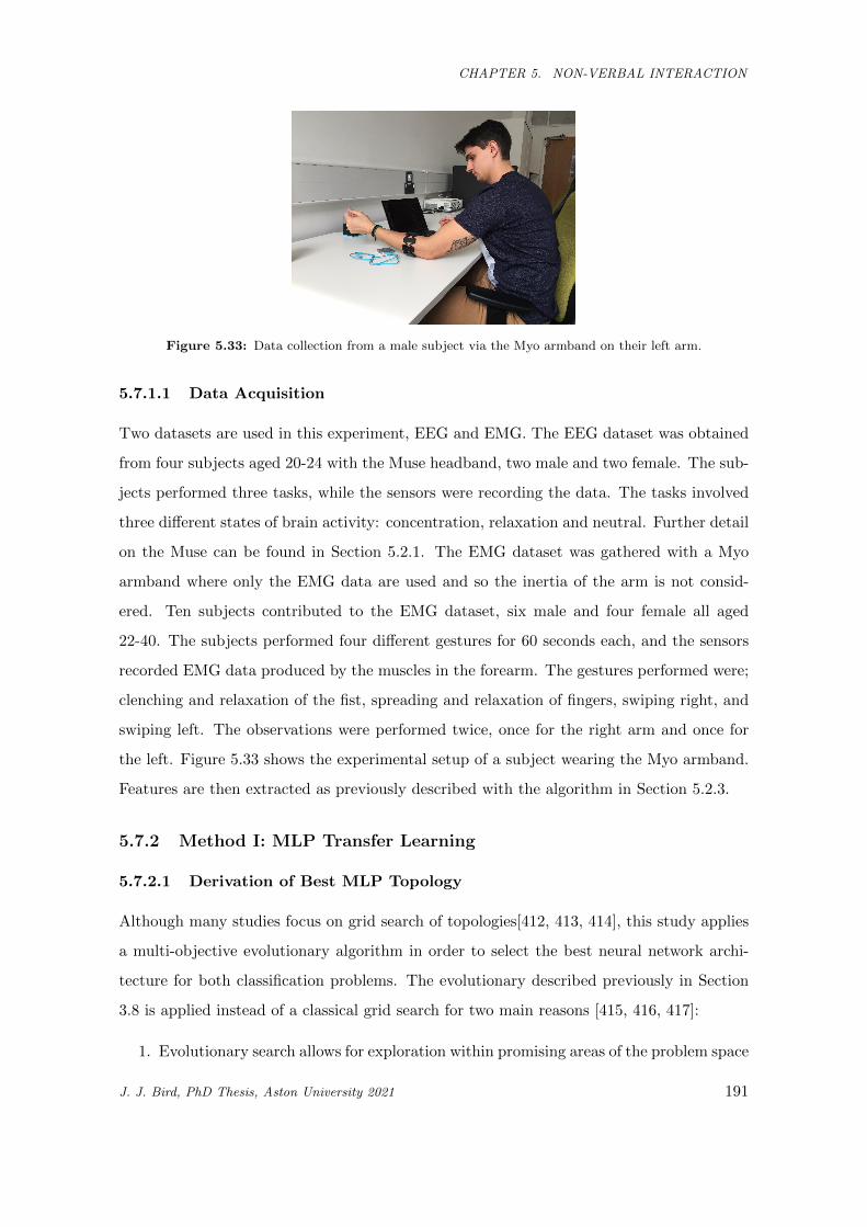
CHAPTER 5. NON-VERBAL INTERACTION
Figure 5.33: Data collection from a male subject via the Myo armband on their left arm.
5.7.1.1 Data Acquisition
Two datasets are used in this experiment, EEG and EMG. The EEG dataset was obtained
from four subjects aged 20-24 with the Muse headband, two male and two female. The sub-
jects performed three tasks, while the sensors were recording the data. The tasks involved
three different states of brain activity: concentration, relaxation and neutral. Further detail
on the Muse can be found in Section 5.2.1. The EMG dataset was gathered with a Myo
armband where only the EMG data are used and so the inertia of the arm is not consid-
ered. Ten subjects contributed to the EMG dataset, six male and four female all aged
22-40. The subjects performed four different gestures for 60 seconds each, and the sensors
recorded EMG data produced by the muscles in the forearm. The gestures performed were;
clenching and relaxation of the fist, spreading and relaxation of fingers, swiping right, and
swiping left. The observations were performed twice, once for the right arm and once for
the left. Figure 5.33 shows the experimental setup of a subject wearing the Myo armband.
Features are then extracted as previously described with the algorithm in Section 5.2.3.
5.7.2 Method I: MLP Transfer Learning
5.7.2.1 Derivation of Best MLP Topology
Although many studies focus on grid search of topologies[412, 413, 414], this study applies
a multi-objective evolutionary algorithm in order to select the best neural network archi-
tecture for both classification problems. The evolutionary described previously in Section
3.8 is applied instead of a classical grid search for two main reasons [415, 416, 417]:
1. Evolutionary search allows for exploration within promising areas of the problem space
J. J. Bird, PhD Thesis, Aston University 2021 191
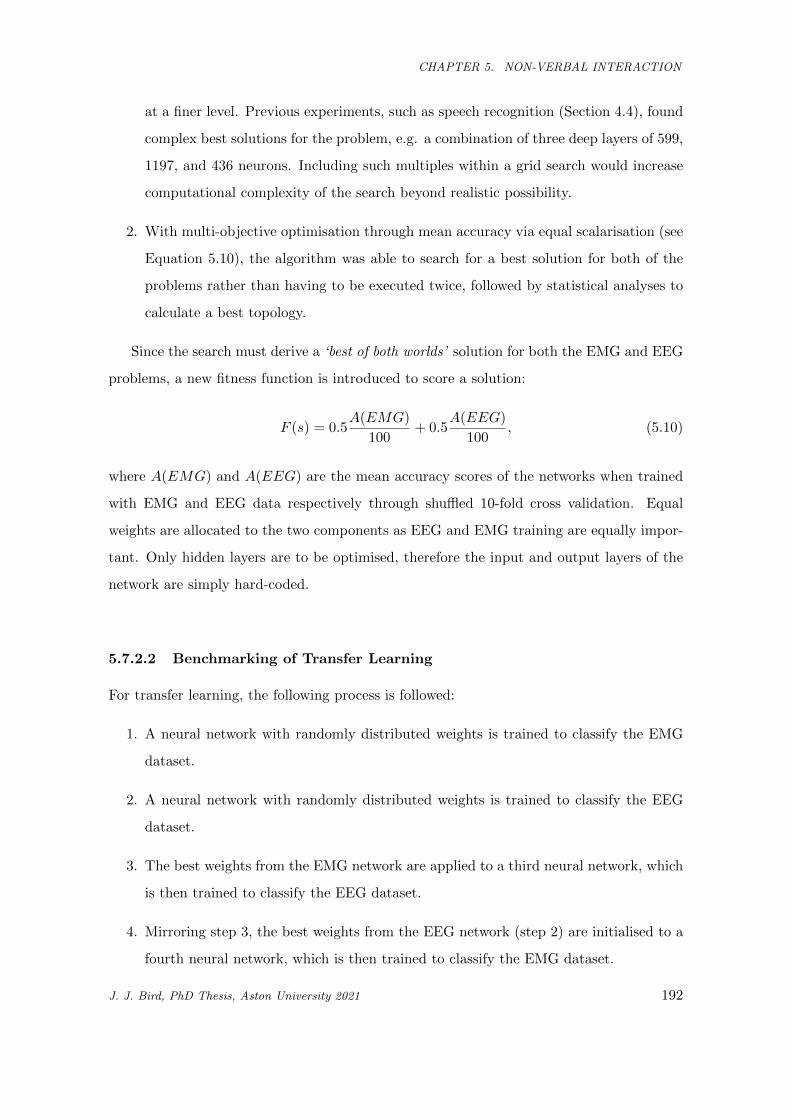
CHAPTER 5. NON-VERBAL INTERACTION
at a finer level. Previous experiments, such as speech recognition (Section 4.4), found
complex best solutions for the problem, e.g. a combination of three deep layers of 599,
1197, and 436 neurons. Including such multiples within a grid search would increase
computational complexity of the search beyond realistic possibility.
2. With multi-objective optimisation through mean accuracy via equal scalarisation (see
Equation 5.10), the algorithm was able to search for a best solution for both of the
problems rather than having to be executed twice, followed by statistical analyses to
calculate a best topology.
Since the search must derive a ‘best of both worlds’ solution for both the EMG and EEG
problems, a new fitness function is introduced to score a solution:
F (s) = 0.5A(EMG)
100+ 0.5
A(EEG)
100, (5.10)
where A(EMG) and A(EEG) are the mean accuracy scores of the networks when trained
with EMG and EEG data respectively through shuffled 10-fold cross validation. Equal
weights are allocated to the two components as EEG and EMG training are equally impor-
tant. Only hidden layers are to be optimised, therefore the input and output layers of the
network are simply hard-coded.
5.7.2.2 Benchmarking of Transfer Learning
For transfer learning, the following process is followed:
1. A neural network with randomly distributed weights is trained to classify the EMG
dataset.
2. A neural network with randomly distributed weights is trained to classify the EEG
dataset.
3. The best weights from the EMG network are applied to a third neural network, which
is then trained to classify the EEG dataset.
4. Mirroring step 3, the best weights from the EEG network (step 2) are initialised to a
fourth neural network, which is then trained to classify the EMG dataset.
J. J. Bird, PhD Thesis, Aston University 2021 192
CHAPTER 5. NON-VERBAL INTERACTION
Figure 5.34: 30 Samples of EEG as 31x31 Images. Top row shows relaxed, middle row shows neutral, andbottom row shows concentrating.
Figure 5.35: 40 Samples of EMG as 31x31 Images. Top row shows close fist, second row shows openfingers, third row shows wave in and bottom row shows wave out.
The four networks are then compared. EEG to EMG-EEG and EMG to EEG-EMG in order
to discern whether knowledge has been transferred. If higher starts, curves, and asymptotes
are observed, then knowledge is considered succesfully transferred between the two domains.
5.7.3 Method II: CNN Transfer Learning
5.7.3.1 Representing Biological Waves as Images
In order to generate a square matrix, after the feature extraction process, the final 28
attributes are removed from each dataset. This is done because 961 is the closest square
number within the attribute set (31x31) and the final attributes are chosen in order to retain
identical inputs to the networks for both datasets. After normalisation of all attributes
between the values of 0 and 255, they are then projected as 31px square images. Examples
of waves projected into visual space can be observed in Figures 5.34 and 5.35. Though
padding would be applied in the situation where a square reshape is not possible (if square
J. J. Bird, PhD Thesis, Aston University 2021 193
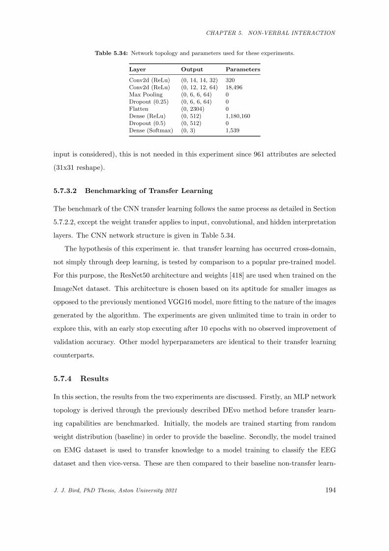
CHAPTER 5. NON-VERBAL INTERACTION
Table 5.34: Network topology and parameters used for these experiments.
Layer Output Parameters
Conv2d (ReLu) (0, 14, 14, 32) 320Conv2d (ReLu) (0, 12, 12, 64) 18,496Max Pooling (0, 6, 6, 64) 0Dropout (0.25) (0, 6, 6, 64) 0Flatten (0, 2304) 0Dense (ReLu) (0, 512) 1,180,160Dropout (0.5) (0, 512) 0Dense (Softmax) (0, 3) 1,539
input is considered), this is not needed in this experiment since 961 attributes are selected
(31x31 reshape).
5.7.3.2 Benchmarking of Transfer Learning
The benchmark of the CNN transfer learning follows the same process as detailed in Section
5.7.2.2, except the weight transfer applies to input, convolutional, and hidden interpretation
layers. The CNN network structure is given in Table 5.34.
The hypothesis of this experiment ie. that transfer learning has occurred cross-domain,
not simply through deep learning, is tested by comparison to a popular pre-trained model.
For this purpose, the ResNet50 architecture and weights [418] are used when trained on the
ImageNet dataset. This architecture is chosen based on its aptitude for smaller images as
opposed to the previously mentioned VGG16 model, more fitting to the nature of the images
generated by the algorithm. The experiments are given unlimited time to train in order to
explore this, with an early stop executing after 10 epochs with no observed improvement of
validation accuracy. Other model hyperparameters are identical to their transfer learning
counterparts.
5.7.4 Results
In this section, the results from the two experiments are discussed. Firstly, an MLP network
topology is derived through the previously described DEvo method before transfer learn-
ing capabilities are benchmarked. Initially, the models are trained starting from random
weight distribution (baseline) in order to provide the baseline. Secondly, the model trained
on EMG dataset is used to transfer knowledge to a model training to classify the EEG
dataset and then vice-versa. These are then compared to their baseline non-transfer learn-
J. J. Bird, PhD Thesis, Aston University 2021 194
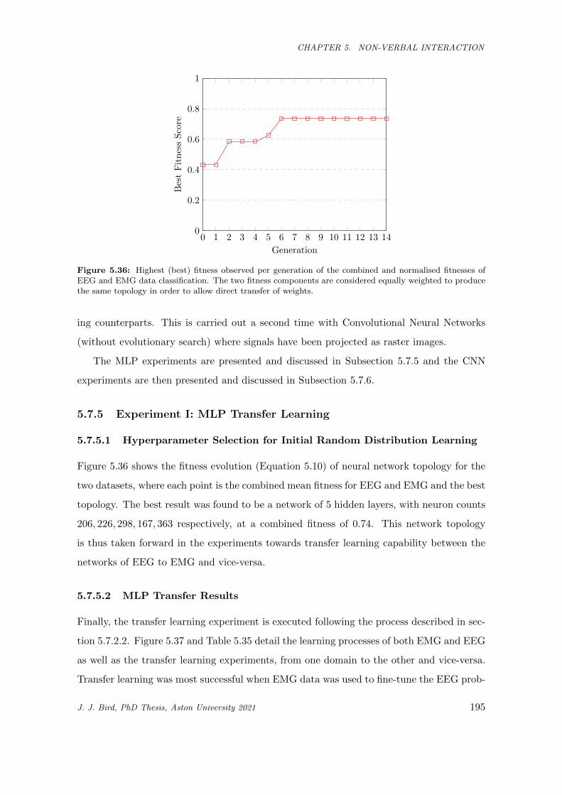
CHAPTER 5. NON-VERBAL INTERACTION
0 1 2 3 4 5 6 7 8 9 10 11 12 13 140
0.2
0.4
0.6
0.8
1
Generation
BestFitnessScore
Figure 5.36: Highest (best) fitness observed per generation of the combined and normalised fitnesses ofEEG and EMG data classification. The two fitness components are considered equally weighted to producethe same topology in order to allow direct transfer of weights.
ing counterparts. This is carried out a second time with Convolutional Neural Networks
(without evolutionary search) where signals have been projected as raster images.
The MLP experiments are presented and discussed in Subsection 5.7.5 and the CNN
experiments are then presented and discussed in Subsection 5.7.6.
5.7.5 Experiment I: MLP Transfer Learning
5.7.5.1 Hyperparameter Selection for Initial Random Distribution Learning
Figure 5.36 shows the fitness evolution (Equation 5.10) of neural network topology for the
two datasets, where each point is the combined mean fitness for EEG and EMG and the best
topology. The best result was found to be a network of 5 hidden layers, with neuron counts
206, 226, 298, 167, 363 respectively, at a combined fitness of 0.74. This network topology
is thus taken forward in the experiments towards transfer learning capability between the
networks of EEG to EMG and vice-versa.
5.7.5.2 MLP Transfer Results
Finally, the transfer learning experiment is executed following the process described in sec-
tion 5.7.2.2. Figure 5.37 and Table 5.35 detail the learning processes of both EMG and EEG
as well as the transfer learning experiments, from one domain to the other and vice-versa.
Transfer learning was most successful when EMG data was used to fine-tune the EEG prob-
J. J. Bird, PhD Thesis, Aston University 2021 195
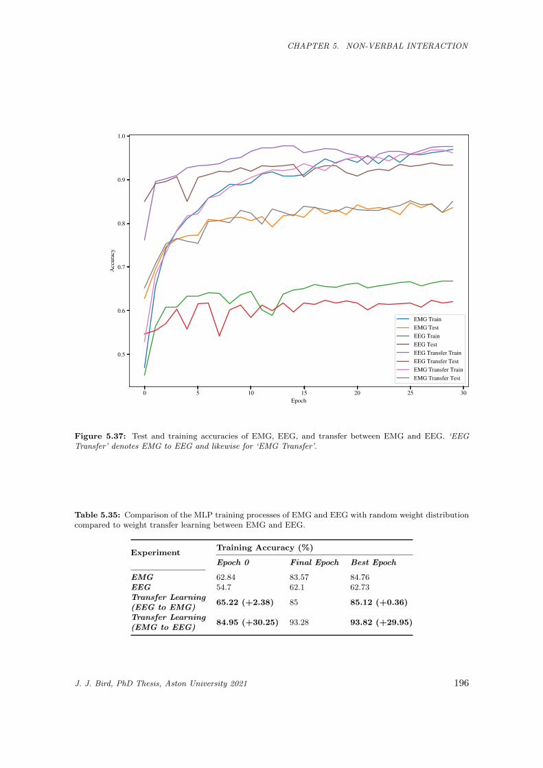
CHAPTER 5. NON-VERBAL INTERACTION
0 5 10 15 20 25 30Epoch
0.5
0.6
0.7
0.8
0.9
1.0
Accu
racy
EMG TrainEMG TestEEG TrainEEG TestEEG Transfer TrainEEG Transfer TestEMG Transfer TrainEMG Transfer Test
Figure 5.37: Test and training accuracies of EMG, EEG, and transfer between EMG and EEG. ‘EEGTransfer’ denotes EMG to EEG and likewise for ‘EMG Transfer’.
Table 5.35: Comparison of the MLP training processes of EMG and EEG with random weight distributioncompared to weight transfer learning between EMG and EEG.
ExperimentTraining Accuracy (%)
Epoch 0 Final Epoch Best Epoch
EMG 62.84 83.57 84.76EEG 54.7 62.1 62.73Transfer Learning(EEG to EMG)
65.22 (+2.38) 85 85.12 (+0.36)
Transfer Learning(EMG to EEG)
84.95 (+30.25) 93.28 93.82 (+29.95)
J. J. Bird, PhD Thesis, Aston University 2021 196
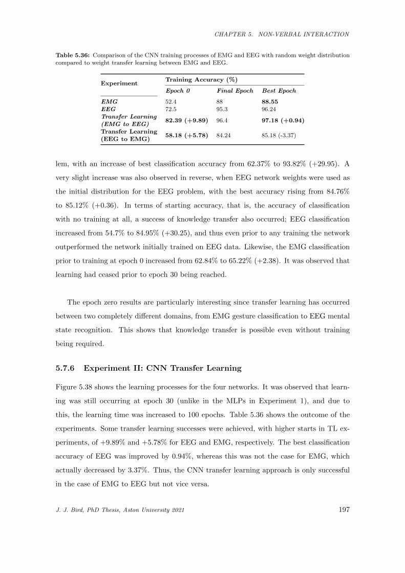
CHAPTER 5. NON-VERBAL INTERACTION
Table 5.36: Comparison of the CNN training processes of EMG and EEG with random weight distributioncompared to weight transfer learning between EMG and EEG.
ExperimentTraining Accuracy (%)
Epoch 0 Final Epoch Best Epoch
EMG 52.4 88 88.55EEG 72.5 95.3 96.24Transfer Learning(EMG to EEG)
82.39 (+9.89) 96.4 97.18 (+0.94)
Transfer Learning(EEG to EMG)
58.18 (+5.78) 84.24 85.18 (-3.37)
lem, with an increase of best classification accuracy from 62.37% to 93.82% (+29.95). A
very slight increase was also observed in reverse, when EEG network weights were used as
the initial distribution for the EEG problem, with the best accuracy rising from 84.76%
to 85.12% (+0.36). In terms of starting accuracy, that is, the accuracy of classification
with no training at all, a success of knowledge transfer also occurred; EEG classification
increased from 54.7% to 84.95% (+30.25), and thus even prior to any training the network
outperformed the network initially trained on EEG data. Likewise, the EMG classification
prior to training at epoch 0 increased from 62.84% to 65.22% (+2.38). It was observed that
learning had ceased prior to epoch 30 being reached.
The epoch zero results are particularly interesting since transfer learning has occurred
between two completely different domains, from EMG gesture classification to EEG mental
state recognition. This shows that knowledge transfer is possible even without training
being required.
5.7.6 Experiment II: CNN Transfer Learning
Figure 5.38 shows the learning processes for the four networks. It was observed that learn-
ing was still occurring at epoch 30 (unlike in the MLPs in Experiment 1), and due to
this, the learning time was increased to 100 epochs. Table 5.36 shows the outcome of the
experiments. Some transfer learning successes were achieved, with higher starts in TL ex-
periments, of +9.89% and +5.78% for EEG and EMG, respectively. The best classification
accuracy of EEG was improved by 0.94%, whereas this was not the case for EMG, which
actually decreased by 3.37%. Thus, the CNN transfer learning approach is only successful
in the case of EMG to EEG but not vice versa.
J. J. Bird, PhD Thesis, Aston University 2021 197
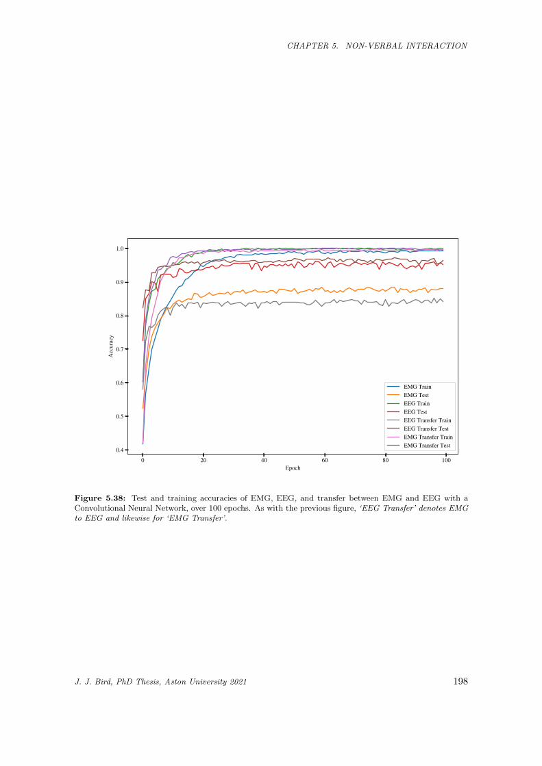
CHAPTER 5. NON-VERBAL INTERACTION
0 20 40 60 80 100Epoch
0.4
0.5
0.6
0.7
0.8
0.9
1.0
Accu
racy
EMG TrainEMG TestEEG TrainEEG TestEEG Transfer TrainEEG Transfer TestEMG Transfer TrainEMG Transfer Test
Figure 5.38: Test and training accuracies of EMG, EEG, and transfer between EMG and EEG with aConvolutional Neural Network, over 100 epochs. As with the previous figure, ‘EEG Transfer’ denotes EMGto EEG and likewise for ‘EMG Transfer’.
J. J. Bird, PhD Thesis, Aston University 2021 198
CHAPTER 5. NON-VERBAL INTERACTION
Table 5.37: Best CNN accuracy observed for ResNet50, Baseline (Non-Transfer), and Transfer Learning.
Best CNN Accuracy Observed (%)
ResNet50 Baseline Transfer LearningEEG EMG EEG EMG EEG EMG92.34 74.92 96.24 88.55 97.18 85.18
It is important to note that previously, the One Rule Random Forest approach (Section
5.3) gained 87.16% accuracy and the image representation and CNN approach (Section 5.4)
gained 89.38% accuracy on EEG data. Our network is competitive at 82.39% accuracy on
the same dataset with no training whatsoever, using simply the weights from the EMG net-
work. Similarly, it is also important to note that the final accuracy of 97.18% substantially
outperforms these previous approaches.
5.7.6.1 Comparison to ResNet50
For comparison of transfer quality, the ResNet 50 CNN architecture is used. Table 5.37
shows that the ResNet50 achieves weaker results for both problems. The ResNet50 ar-
chitecture was observed to stop improving after 35 and 39 epochs for EEG and EMG
respectively, similarly to the behaviour of our architecture shown in Figure 5.38.
5.8 Summary and Conclusion
The experiments and results presented in this chapter have led to several non-verbal com-
munication abilities for the HRI framework. Initially, Section 5.3 suggested DEvo, a Deep
Evolutionary approach to optimise and classify complex signals using bio-inspired com-
puting methods in the whole pipeline, from feature selection to classification. For mental
state and mental emotional state classification of EEG brainwaves and their mathematical
features, the two best models were selected. Firstly, a more accurate AdaBoosted LSTM,
that took more time and resources to train in comparison to other methods, but man-
aged to attain accuracies of 84.44% and 97.06% for the two first datasets (attentional and
emotional state classification). Secondly, a AdaBoosted Multilayer Perceptron that was op-
timised using a hyper-heuristic evolutionary algorithm. Although its classification accuracy
was slightly lower than that of the AdaBoosted LSTM (79.7% and 96.23% for the same
J. J. Bird, PhD Thesis, Aston University 2021 199
CHAPTER 5. NON-VERBAL INTERACTION
two experiments), less time was required for training. For the MindBigData digits dataset,
the most accurate model was an Adaptive Boosted version of the DEvo optimised MLP,
which achieved an accuracy of 30%. For this problem, none of the LSTMs were able to
achieve any meaningful nor useful results, but the DEvo MLP approach saved time, and
also produced results that were somewhat useful. Results were noted to be impressive for
application due to the high classification ability along with the reduction of resource usage
- real-time training from individuals would be possible and thus provide a more accurate
EEG-based product to the consumer, for example, in real-time monitoring of mental state
for the grading of meditation or yoga session quality. Real time communication would also
be possible in human-computer interaction where the brain activity acts as a degree of in-
put. The goal of the experiments were successfully achieved, the DEvo approach has led to
an optimised, resource-light model that closely matches that to an extremely resource heavy
deep learning model, losing a small amount of accuracy but computing in approximately
10% of the time, except for in one case in which it far outperformed its competitor models.
The aforementioned models were trained on a set of attributes that were selected with a
bioinspired evolutionary algorithm. The success of these processes led to future work sug-
gestions, which follow the pattern of further bioinspired optimisation applications within
the field of machine learning. Future work should also consider, for better application of the
process within the field of Electroencephalography, a much larger collection of data from a
considerably more diverse range of subjects in order to better model the classifier optimi-
sation for the thought pattern of a global population rather than the subjects encompassed
within this study.
Following on from these experiments, Section 5.4 then explored the possibility of using
image recognition techniques for EEG signal processing. 729 features were selected to
directly compare 2D and 3D visual space for EEG classification, since 729 can be used
to make both a perfect square and cube. Experiments showed the superiority of the 2-
Dimensional approach and there are of course many more numbers within the bounds of
the attribute set that make only a perfect square, 1273 to be exact. If cube comparison is
discarded, the image size could be explored to test whether there is a better set of results
totalling either more or fewer than the 729 that was chosen. The feature extraction for
the 64-channel dataset produced 23,488 attributes and thus further studies on this could
attempt to compare different sized images and cubes due to the abundance of features.
J. J. Bird, PhD Thesis, Aston University 2021 200
CHAPTER 5. NON-VERBAL INTERACTION
Furthermore, the method of reshaping to 2D and 3D through the order of their feature
selection scores was performed in a relatively simple fashion for the purposes of preliminary
exploration. In future studies, due to the success found in this work, the method of reshaping
and ordering of the attributes within the shape will be studied considering the reshaping
method an additional network hyperparameter. This presents a combinatorial optimisation
problem that should be further explored and solved in order to present more scientifically
sound methods for reshaping. In addition, in future, it would be useful to explore other
methods of feature extraction using the CNN model. In Section 5.4, the approach presented
was compared to statistical models which also had the same features as input - although
this would not be possible in the raw signal domain, the raw signals may be more useful for
convolutional neural networks to learn from in future benchmarking experiments. Another
limitation of the study is that the unseen data was restricted to both holdout test sets and
unseen subjects, in future a further dataset should be collected in order to enable testing
on a larger amount of unseen data. As previously described, the main limitation of the
work in Section 5.4 is the method of reshaping, three methods were explored which were
dictated by the score metrics of three different dimensionality reduction techniques. In
the future, a combinatorial optimisation algorithm could be used with CNN classification
metrics as a function fitness to optimise. Future work could specifically explore the effects
of reshaping on CNNs operating in different numbers of spatial dimensions and thus then
how this may be useful for future tasks. The techniques were applied generally to four
and 64-channel EEG recordings, thus applied to datasets of much different width (given
that temporal techniques are extracted from each electrode), and future work could explore
if differing successful techniques could be applied with either a task or electrode count in
mind. Datasets with larger numbers of subjects and leave-one-subject-out testing could
also be explored in future works to discern whether these models improve the ability of
unseen subject classification or whether calibration is required. To summarise Section 5.4,
initially, nine preliminary deep learning experiments were carried out twice for three EEG
datasets. Three in 2-Dimensional space and three in 3-Dimensional space and compared.
In the cases of attention and emotional state, the 2D CNN outperforms the 3D CNN when
rule-based and entropy-based feature selection is performed, respectively. On the other
hand, for eye state with a 64-channel EEG, the 3D CNN produced the best accuracy when
features were selected via their Symmetrical Uncertainty. The best 2D and 3D models for
J. J. Bird, PhD Thesis, Aston University 2021 201
CHAPTER 5. NON-VERBAL INTERACTION
each were then taken forward for topology optimisation, and finally, to prevent overfitting,
said topologies were validated using 10-fold cross validation. Final results showed that the
data preprocessing methods not only retained their best overall score, but all were improved
upon after topology optimisation and subsequent k-fold cross validation.
Towards real-time HRI via hand gestures, Section 5.5 explored transfer learning tech-
niques to improve gesture recognition via EMG signals. In the calibration experiment,
error rates were found to be extremely low. Accuracy measurements exceeded the original
benchmarks and thus further experimentation is required to explore this. Calibration was
performed for a limited group of four subjects, further experimentation should explore a
more general affect when a larger group of participants are considered. Towards the end of
Section 5.5, preliminary benchmarks were presented for potential application of the induc-
tive and supervised transductive transfer learning calibration process. The 20 Questions
game with a Pepper Robot was possible with 15 seconds of calibration data and 5 seconds
of answering time per question, and predictions were at 100% for two subjects in two dif-
ferent experimental runs. Further work would could both explore more subjects as well as
attempt to perform this task with shorter answering time, i.e., a deeper exploration into
how much data is enough for a confident prediction. For example, rather than the simplistic
most common class Random Forest approach, a more complex system of meta-classification
could prove more useful as the pattern of error may be useful also for prediction; if this were
so, then it stands to reason that confident classification could be enabled sooner than the
5-second mark. Additionally, when a a best-case paradigm is confirmed, the method could
then be compared to other sensory techniques such as image/video classification for gesture
recognition. Furthermore, should the said method be viable, then a multimodal approach
could also be explored to fuse both visual and EMG data. This section showed that the
proposed transfer learning system is viable to be applied to the ternary classification prob-
lem presented. Future work could explore the robustness of this approach to problems of
additional classes and gestures in order to compare how the results are affected when more
problems are introduced. To summarise Section 5.5, the work firstly found that a voting
ensemble was a strong performer for the classification of gesture but failed to generalise to
new data. With the inductive and transductive transfer learning calibration approach, the
best model for generalisation of new data was a Random Forest technique which achieved
relatively high accuracy. After gathering data from a subject for only 5 seconds, the model
J. J. Bird, PhD Thesis, Aston University 2021 202
CHAPTER 5. NON-VERBAL INTERACTION
could confidently classify the gesture at 100% accuracy through the most common class-
based Random Forest classifier. Since high accuracies were achieved by the transfer learning
approach in this work when compared to the state-of-the-art related works and the pro-
prietary MYO system, future applications could be enabled with this approach towards a
much higher resolution of input than is currently available with the MYO system.
Two other methods were also explored for the improvement of signal classification, ulti-
mately leading to better HRI abilities. The first was data augmentation, which was explored
in Section 5.6. The study presented multiple experiments with real and synthetic biological
signals to ascertain whether classification algorithms can be improved by considering data
generated by the GPT-2 model. The first experiments showed that although the data are
different, i.e., real and synthetic data were comparatively unique, a model trained on one of
the two sets of signals shows promising results in being able to classify the other. Thus the
GPT-2 model is able to generate relatively realistic data which holds useful information that
can be learnt from for application to real data. An SVM trained on synthetic EEG data
was observed to classify real data at 74.71% accuracy. Following on from this observation,
experiments then showed that several learning algorithms of differing statistical natures
were improved for EEG classification when the training data was augmented by GPT-2.
The main hypothesis that this section has argued through the experiments performed, is
that synthetic biological signals output by a generative attention-based transformer hold
enough knowledge for data augmentation to improve learning algorithms for classification
of real biological signal data. In the future, larger datasets could be leveraged and thus deep
learning would be a realistic possibility for classification, where deep learning processes are
similarly augmented with GPT-2 data. Finally, given that this work showed promise in
terms of the model architecture itself, similar models could also be benchmarked in terms
of their ability to create augmented training datasets, e.g. BART, CTRL, Transformer-XL
and XLNet. The second method of model improvement that was explored was cross-domain
transfer learning in Section 5.7. The study demonstrated that cross-domain transfer learn-
ing is possible between the domains of electroencephalography and electromyography via
the electrical signals produced by the frontal lobe of the brain and forearm muscles. Cross-
domain transfer learning with EMG to EEG and vice versa has not been explored before
in the related literature prior to these experiments. Limited selection of network topologies
was performed through a single multi-objective evolutionary search. With the possibility
J. J. Bird, PhD Thesis, Aston University 2021 203
CHAPTER 5. NON-VERBAL INTERACTION
of a local minimum being encountered and stagnation occurring, further executions of the
search should be performed in a subsequent study in order to explore the problem space
and thus reduce the chance of stagnation. Scalarisation was considered equal between the
two datasets, although the EMG dataset was more diverse and much larger than the EEG
dataset and thus alternative scalars with preference to either dataset should also be bench-
marked. Future work could also involve the possibility of cross-domain transfer learning
in multiple biological signal domains, such as including other areas of the muscular sys-
tem and brain, and additionally, other domains such as electrocardiography. The potential
for transfer learning between these domains should be applied in Human-Machine Interac-
tion in the future, since the application of a framework as described here shows not only
the advantage of improved accuracy of classification, but additionally, the derivation of a
less computationally expensive process compared to learning from scratch. To summarise,
Section 5.7 argued that, through initial weight distribution, cross-domain transfer learn-
ing between two biological signal domains is possible and, in some cases, has a positive
effect on machine learning. Identical mathematical features were extracted from the waves
to provide a stationary description fit for classification, and transfer between features was
also noted. Initial pre-training abilities were higher than random weight distribution, the
learning curves and final classification abilities for both domains were also better, indicating
that useful knowledge had been shared between both domains during the transfer learning
process. The exploration of the possibility of transfer of knowledge from/to other biological
signal domains such as ECG is also an exciting topic for future study.
To finally conclude this chapter, as was noted in the previous chapter, the experiments
performed have led to several new technologies and modules to be implemented within the
overall framework when all works are unified. Classification of concentrative and emotional
states from EEG data are now possible, with varying levels of complexity and often rela-
tive ability, which are useful since the framework could be operating with varying levels of
computational complexity - for example, the CNN approach was strong for mental state
recognition but a weak machine may prefer to use the Random Forest or Extreme Gradient
Boosting approaches which achieve a lower ability but through a much less complex model.
In addition to this ability, the interpretation of gestures is now possible for affirmative or
negative responses via electromyography as another mode of social interaction with ma-
chines. Towards the end of this chapter, it was also discovered that transfer learning was
J. J. Bird, PhD Thesis, Aston University 2021 204

CHAPTER 5. NON-VERBAL INTERACTION
possible between the two signal domains and useful knowledge could be shared between
them. Finally, it was then discovered that the classification of signals was improved when
the model was exposed to synthetic data augmentation via training generative transformer
models.
J. J. Bird, PhD Thesis, Aston University 2021 205
CHAPTER 6. MULTIMODALITY INTERACTION
Chapter 6
Multimodality Human-Robot
Interaction
6.1 Introduction
In Machine Learning, Multimodality is the application of multiple, differing inputs towards
a common goal [419]. To give a specific example in the field, a human’s emotional state
(the common goal) can be interpreted and predicted by considering multiple physiological
signals (as in, multiple, differing inputs) to improve the predictive ability of a model when
classifying emotional states[420].
In this Chapter, several experiments are performed to enable Multimodality learning
within the framework that is ultimately derived in Chapter 7. The three experiments focus
on the fusion of audio and images to improve scene recognition in Section 6.2, the transfer of
knowledge from simulated environments to real environments to improve scene recognition
in Section 6.3, and then the fusion of image and Leap Motion data to improve a Sign
Language Recognition system’s robustness when interpreting new subjects in Section 6.4.
6.2 Multimodality Late Fusion for Scene Classification
The novelty of this study consists in a multi-modal approach to scene classification, where
image and audio complement each other in a process of deep late fusion. Specifically, it is
found that situations where a single model may be confused by anomalous data points are
now corrected through an emerging higher order integration. Prominent examples include
J. J. Bird, PhD Thesis, Aston University 2021 206
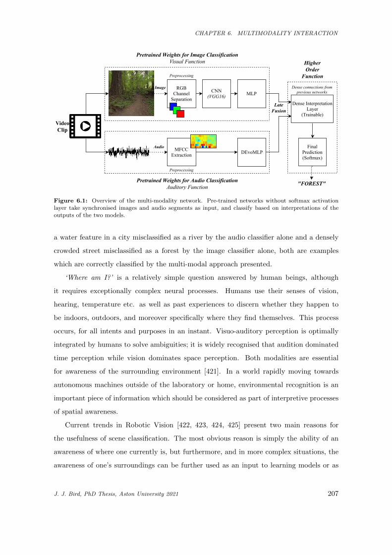
CHAPTER 6. MULTIMODALITY INTERACTION
CNN(VGG16)
DEvoMLP
MLP
DenseInterpretationLayer
(Trainable)
FinalPrediction(Softmax)
Audio
Image
PretrainedWeightsforImageClassificationVisualFunction
PretrainedWeightsforAudioClassificationAuditoryFunction
MFCCExtraction
HigherOrder
Function
VideoClip
RGBChannelSeparation
Preprocessing
Preprocessing
Denseconnectionsfrompreviousnetworks
LateFusion
"FOREST"
Figure 6.1: Overview of the multi-modality network. Pre-trained networks without softmax activationlayer take synchronised images and audio segments as input, and classify based on interpretations of theoutputs of the two models.
a water feature in a city misclassified as a river by the audio classifier alone and a densely
crowded street misclassified as a forest by the image classifier alone, both are examples
which are correctly classified by the multi-modal approach presented.
‘Where am I?’ is a relatively simple question answered by human beings, although
it requires exceptionally complex neural processes. Humans use their senses of vision,
hearing, temperature etc. as well as past experiences to discern whether they happen to
be indoors, outdoors, and moreover specifically where they find themselves. This process
occurs, for all intents and purposes in an instant. Visuo-auditory perception is optimally
integrated by humans to solve ambiguities; it is widely recognised that audition dominated
time perception while vision dominates space perception. Both modalities are essential
for awareness of the surrounding environment [421]. In a world rapidly moving towards
autonomous machines outside of the laboratory or home, environmental recognition is an
important piece of information which should be considered as part of interpretive processes
of spatial awareness.
Current trends in Robotic Vision [422, 423, 424, 425] present two main reasons for
the usefulness of scene classification. The most obvious reason is simply the ability of an
awareness of where one currently is, but furthermore, and in more complex situations, the
awareness of one’s surroundings can be further used as an input to learning models or as
J. J. Bird, PhD Thesis, Aston University 2021 207
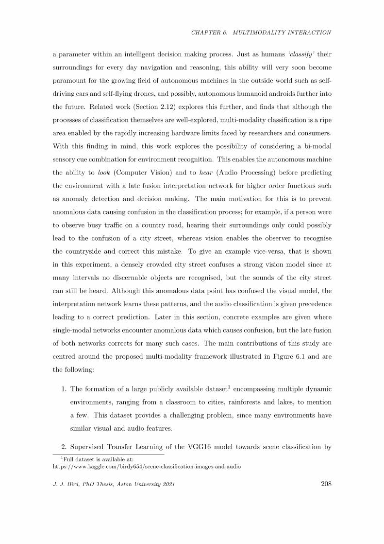
CHAPTER 6. MULTIMODALITY INTERACTION
a parameter within an intelligent decision making process. Just as humans ‘classify’ their
surroundings for every day navigation and reasoning, this ability will very soon become
paramount for the growing field of autonomous machines in the outside world such as self-
driving cars and self-flying drones, and possibly, autonomous humanoid androids further into
the future. Related work (Section 2.12) explores this further, and finds that although the
processes of classification themselves are well-explored, multi-modality classification is a ripe
area enabled by the rapidly increasing hardware limits faced by researchers and consumers.
With this finding in mind, this work explores the possibility of considering a bi-modal
sensory cue combination for environment recognition. This enables the autonomous machine
the ability to look (Computer Vision) and to hear (Audio Processing) before predicting
the environment with a late fusion interpretation network for higher order functions such
as anomaly detection and decision making. The main motivation for this is to prevent
anomalous data causing confusion in the classification process; for example, if a person were
to observe busy traffic on a country road, hearing their surroundings only could possibly
lead to the confusion of a city street, whereas vision enables the observer to recognise
the countryside and correct this mistake. To give an example vice-versa, that is shown
in this experiment, a densely crowded city street confuses a strong vision model since at
many intervals no discernable objects are recognised, but the sounds of the city street
can still be heard. Although this anomalous data point has confused the visual model, the
interpretation network learns these patterns, and the audio classification is given precedence
leading to a correct prediction. Later in this section, concrete examples are given where
single-modal networks encounter anomalous data which causes confusion, but the late fusion
of both networks corrects for many such cases. The main contributions of this study are
centred around the proposed multi-modality framework illustrated in Figure 6.1 and are
the following:
1. The formation of a large publicly available dataset1 encompassing multiple dynamic
environments, ranging from a classroom to cities, rainforests and lakes, to mention
a few. This dataset provides a challenging problem, since many environments have
similar visual and audio features.
2. Supervised Transfer Learning of the VGG16 model towards scene classification by
1Full dataset is available at:https://www.kaggle.com/birdy654/scene-classification-images-and-audio
J. J. Bird, PhD Thesis, Aston University 2021 208
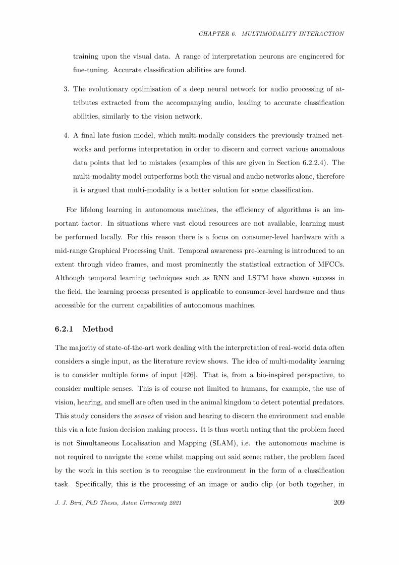
CHAPTER 6. MULTIMODALITY INTERACTION
training upon the visual data. A range of interpretation neurons are engineered for
fine-tuning. Accurate classification abilities are found.
3. The evolutionary optimisation of a deep neural network for audio processing of at-
tributes extracted from the accompanying audio, leading to accurate classification
abilities, similarly to the vision network.
4. A final late fusion model, which multi-modally considers the previously trained net-
works and performs interpretation in order to discern and correct various anomalous
data points that led to mistakes (examples of this are given in Section 6.2.2.4). The
multi-modality model outperforms both the visual and audio networks alone, therefore
it is argued that multi-modality is a better solution for scene classification.
For lifelong learning in autonomous machines, the efficiency of algorithms is an im-
portant factor. In situations where vast cloud resources are not available, learning must
be performed locally. For this reason there is a focus on consumer-level hardware with a
mid-range Graphical Processing Unit. Temporal awareness pre-learning is introduced to an
extent through video frames, and most prominently the statistical extraction of MFCCs.
Although temporal learning techniques such as RNN and LSTM have shown success in
the field, the learning process presented is applicable to consumer-level hardware and thus
accessible for the current capabilities of autonomous machines.
6.2.1 Method
The majority of state-of-the-art work dealing with the interpretation of real-world data often
considers a single input, as the literature review shows. The idea of multi-modality learning
is to consider multiple forms of input [426]. That is, from a bio-inspired perspective, to
consider multiple senses. This is of course not limited to humans, for example, the use of
vision, hearing, and smell are often used in the animal kingdom to detect potential predators.
This study considers the senses of vision and hearing to discern the environment and enable
this via a late fusion decision making process. It is thus worth noting that the problem faced
is not Simultaneous Localisation and Mapping (SLAM), i.e. the autonomous machine is
not required to navigate the scene whilst mapping out said scene; rather, the problem faced
by the work in this section is to recognise the environment in the form of a classification
task. Specifically, this is the processing of an image or audio clip (or both together, in
J. J. Bird, PhD Thesis, Aston University 2021 209
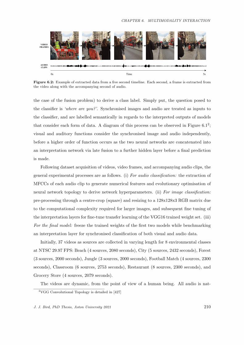
CHAPTER 6. MULTIMODALITY INTERACTION
0s 5sTime
VIDEOFRAMES
AUDIOCLIPS
Figure 6.2: Example of extracted data from a five second timeline. Each second, a frame is extracted fromthe video along with the accompanying second of audio.
the case of the fusion problem) to derive a class label. Simply put, the question posed to
the classifier is ‘where are you?’. Synchronised images and audio are treated as inputs to
the classifier, and are labelled semantically in regards to the interpreted outputs of models
that consider each form of data. A diagram of this process can be observed in Figure 6.12;
visual and auditory functions consider the synchronised image and audio independently,
before a higher order of function occurs as the two neural networks are concatenated into
an interpretation network via late fusion to a further hidden layer before a final prediction
is made.
Following dataset acquisition of videos, video frames, and accompanying audio clips, the
general experimental processes are as follows. (i) For audio classification: the extraction of
MFCCs of each audio clip to generate numerical features and evolutionary optimisation of
neural network topology to derive network hyperparameters. (ii) For image classification:
pre-processing through a centre-crop (square) and resizing to a 128x128x3 RGB matrix due
to the computational complexity required for larger images, and subsequent fine tuning of
the interpretation layers for fine-tune transfer learning of the VGG16 trained weight set. (iii)
For the final model: freeze the trained weights of the first two models while benchmarking
an interpretation layer for synchronised classification of both visual and audio data.
Initially, 37 videos as sources are collected in varying length for 8 environmental classes
at NTSC 29.97 FPS: Beach (4 sources, 2080 seconds), City (5 sources, 2432 seconds), Forest
(3 sources, 2000 seconds), Jungle (3 sources, 2000 seconds), Football Match (4 sources, 2300
seconds), Classroom (6 sources, 2753 seconds), Restaurant (8 sources, 2300 seconds), and
Grocery Store (4 sources, 2079 seconds).
The videos are dynamic, from the point of view of a human being. All audio is nat-
2VGG Convolutional Topology is detailed in [427]
J. J. Bird, PhD Thesis, Aston University 2021 210
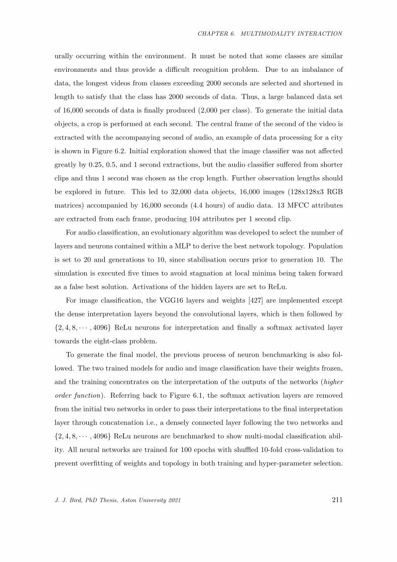
CHAPTER 6. MULTIMODALITY INTERACTION
urally occurring within the environment. It must be noted that some classes are similar
environments and thus provide a difficult recognition problem. Due to an imbalance of
data, the longest videos from classes exceeding 2000 seconds are selected and shortened in
length to satisfy that the class has 2000 seconds of data. Thus, a large balanced data set
of 16,000 seconds of data is finally produced (2,000 per class). To generate the initial data
objects, a crop is performed at each second. The central frame of the second of the video is
extracted with the accompanying second of audio, an example of data processing for a city
is shown in Figure 6.2. Initial exploration showed that the image classifier was not affected
greatly by 0.25, 0.5, and 1 second extractions, but the audio classifier suffered from shorter
clips and thus 1 second was chosen as the crop length. Further observation lengths should
be explored in future. This led to 32,000 data objects, 16,000 images (128x128x3 RGB
matrices) accompanied by 16,000 seconds (4.4 hours) of audio data. 13 MFCC attributes
are extracted from each frame, producing 104 attributes per 1 second clip.
For audio classification, an evolutionary algorithm was developed to select the number of
layers and neurons contained within a MLP to derive the best network topology. Population
is set to 20 and generations to 10, since stabilisation occurs prior to generation 10. The
simulation is executed five times to avoid stagnation at local minima being taken forward
as a false best solution. Activations of the hidden layers are set to ReLu.
For image classification, the VGG16 layers and weights [427] are implemented except
the dense interpretation layers beyond the convolutional layers, which is then followed by
{2, 4, 8, · · · , 4096} ReLu neurons for interpretation and finally a softmax activated layer
towards the eight-class problem.
To generate the final model, the previous process of neuron benchmarking is also fol-
lowed. The two trained models for audio and image classification have their weights frozen,
and the training concentrates on the interpretation of the outputs of the networks (higher
order function). Referring back to Figure 6.1, the softmax activation layers are removed
from the initial two networks in order to pass their interpretations to the final interpretation
layer through concatenation i.e., a densely connected layer following the two networks and
{2, 4, 8, · · · , 4096} ReLu neurons are benchmarked to show multi-modal classification abil-
ity. All neural networks are trained for 100 epochs with shuffled 10-fold cross-validation to
prevent overfitting of weights and topology in both training and hyper-parameter selection.
J. J. Bird, PhD Thesis, Aston University 2021 211
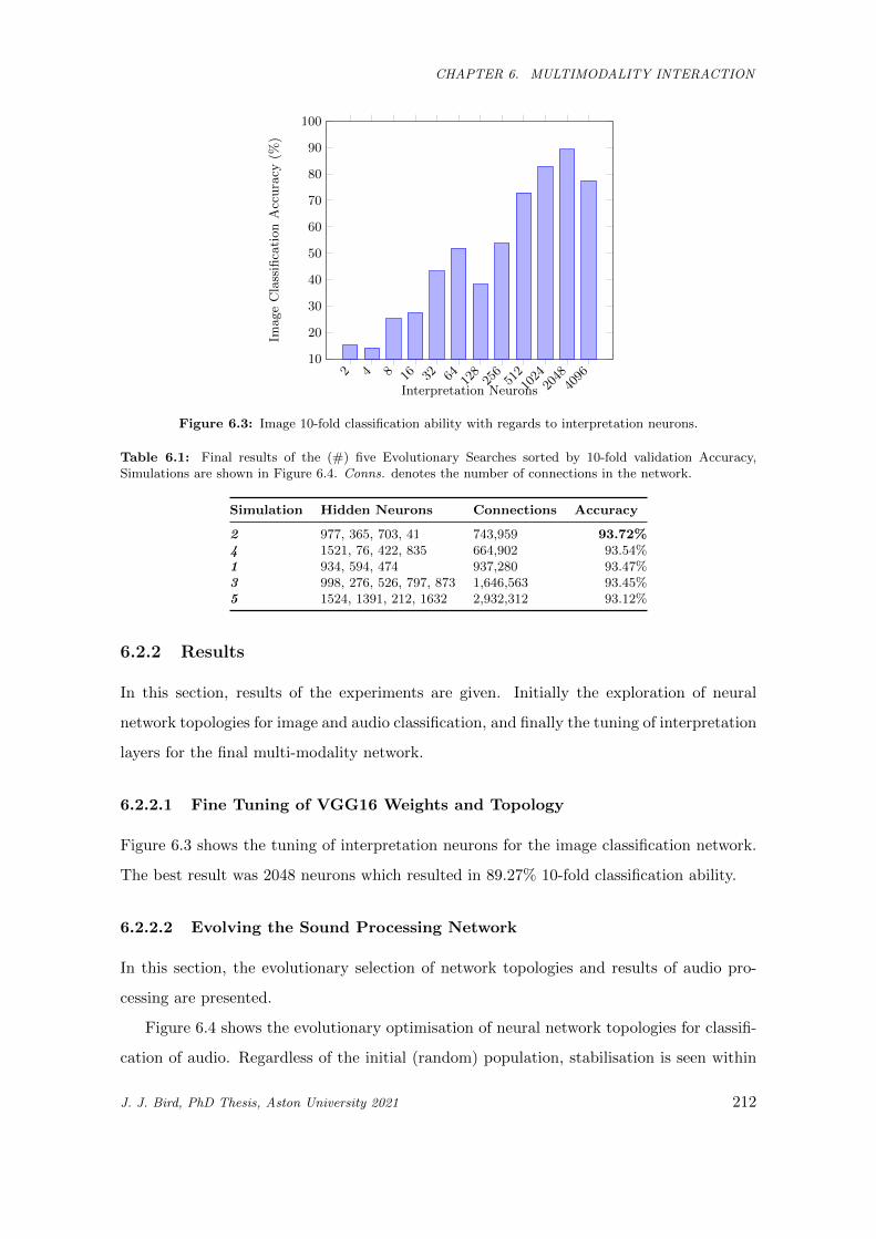
CHAPTER 6. MULTIMODALITY INTERACTION
2 4 8 16 32 64 128
256
51210
2420
4840
9610
20
30
40
50
60
70
80
90
100
Interpretation Neurons
Image
Cla
ssifi
cati
on
Acc
ura
cy(%
)
Figure 6.3: Image 10-fold classification ability with regards to interpretation neurons.
Table 6.1: Final results of the (#) five Evolutionary Searches sorted by 10-fold validation Accuracy,Simulations are shown in Figure 6.4. Conns. denotes the number of connections in the network.
Simulation Hidden Neurons Connections Accuracy
2 977, 365, 703, 41 743,959 93.72%4 1521, 76, 422, 835 664,902 93.54%1 934, 594, 474 937,280 93.47%3 998, 276, 526, 797, 873 1,646,563 93.45%5 1524, 1391, 212, 1632 2,932,312 93.12%
6.2.2 Results
In this section, results of the experiments are given. Initially the exploration of neural
network topologies for image and audio classification, and finally the tuning of interpretation
layers for the final multi-modality network.
6.2.2.1 Fine Tuning of VGG16 Weights and Topology
Figure 6.3 shows the tuning of interpretation neurons for the image classification network.
The best result was 2048 neurons which resulted in 89.27% 10-fold classification ability.
6.2.2.2 Evolving the Sound Processing Network
In this section, the evolutionary selection of network topologies and results of audio pro-
cessing are presented.
Figure 6.4 shows the evolutionary optimisation of neural network topologies for classifi-
cation of audio. Regardless of the initial (random) population, stabilisation is seen within
J. J. Bird, PhD Thesis, Aston University 2021 212
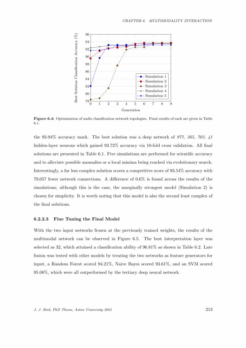
CHAPTER 6. MULTIMODALITY INTERACTION
0 1 2 3 4 5 6 7 8 978
80
82
84
86
88
90
92
94
96
Generation
Bes
tS
olu
tion
Cla
ssifi
cati
on
Acc
ura
cy(%
)Simulation 1
Simulation 2
Simulation 3
Simulation 4
Simulation 5
Figure 6.4: Optimisation of audio classification network topologies. Final results of each are given in Table6.1.
the 92-94% accuracy mark. The best solution was a deep network of 977, 365, 703, 41
hidden-layer neurons which gained 93.72% accuracy via 10-fold cross validation. All final
solutions are presented in Table 6.1. Five simulations are performed for scientific accuracy
and to alleviate possible anomalies or a local minima being reached via evolutionary search.
Interestingly, a far less complex solution scores a competitive score of 93.54% accuracy with
79,057 fewer network connections. A difference of 0.6% is found across the results of the
simulations; although this is the case, the marginally strongest model (Simulation 2) is
chosen for simplicity. It is worth noting that this model is also the second least complex of
the final solutions.
6.2.2.3 Fine Tuning the Final Model
With the two input networks frozen at the previously trained weights, the results of the
multimodal network can be observed in Figure 6.5. The best interpretation layer was
selected as 32, which attained a classification ability of 96.81% as shown in Table 6.2. Late
fusion was tested with other models by treating the two networks as feature generators for
input, a Random Forest scored 94.21%, Naive Bayes scored 93.61%, and an SVM scored
95.08%, which were all outperformed by the tertiary deep neural network.
J. J. Bird, PhD Thesis, Aston University 2021 213
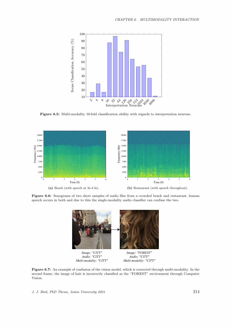
CHAPTER 6. MULTIMODALITY INTERACTION
2 4 8 16 32 64 128
256
51210
2420
4840
9610
20
30
40
50
60
70
80
90
100
Interpretation Neurons
Sce
ne
Cla
ssifi
cati
on
Acc
ura
cy(%
)
Figure 6.5: Multi-modality 10-fold classification ability with regards to interpretation neurons.
(a) Beach (with speech at 3s-4.5s). (b) Restaurant (with speech throughout).
Figure 6.6: Sonograms of two short samples of audio files from a crowded beach and restaurant, humanspeech occurs in both and due to this the single-modality audio classifier can confuse the two.
Image:"CITY"Audio:"CITY"
Multi-modality:"CITY"
Image:"FOREST"Audio:"CITY"
Multi-modality:"CITY"
Figure 6.7: An example of confusion of the vision model, which is corrected through multi-modality. In thesecond frame, the image of hair is incorrectly classified as the “FOREST” environment through ComputerVision.
J. J. Bird, PhD Thesis, Aston University 2021 214
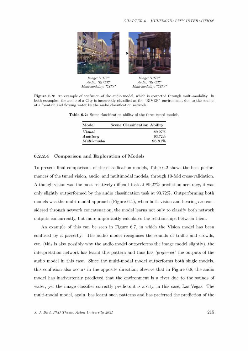
CHAPTER 6. MULTIMODALITY INTERACTION
Image:"CITY"Audio:"RIVER"
Multi-modality:"CITY"
Image:"CITY"Audio:"RIVER"
Multi-modality:"CITY"
Figure 6.8: An example of confusion of the audio model, which is corrected through multi-modality. Inboth examples, the audio of a City is incorrectly classified as the “RIVER” environment due to the soundsof a fountain and flowing water by the audio classification network.
Table 6.2: Scene classification ability of the three tuned models.
Model Scene Classification Ability
Visual 89.27%Auditory 93.72%Multi-modal 96.81%
6.2.2.4 Comparison and Exploration of Models
To present final comparisons of the classification models, Table 6.2 shows the best perfor-
mances of the tuned vision, audio, and multimodal models, through 10-fold cross-validation.
Although vision was the most relatively difficult task at 89.27% prediction accuracy, it was
only slightly outperformed by the audio classification task at 93.72%. Outperforming both
models was the multi-modal approach (Figure 6.1), when both vision and hearing are con-
sidered through network concatenation, the model learns not only to classify both network
outputs concurrently, but more importantly calculates the relationships between them.
An example of this can be seen in Figure 6.7, in which the Vision model has been
confused by a passerby. The audio model recognises the sounds of traffic and crowds,
etc. (this is also possibly why the audio model outperforms the image model slightly), the
interpretation network has learnt this pattern and thus has ‘preferred’ the outputs of the
audio model in this case. Since the multi-modal model outperforms both single models,
this confusion also occurs in the opposite direction; observe that in Figure 6.8, the audio
model has inadvertently predicted that the environment is a river due to the sounds of
water, yet the image classifier correctly predicts it is a city, in this case, Las Vegas. The
multi-modal model, again, has learnt such patterns and has preferred the prediction of the
J. J. Bird, PhD Thesis, Aston University 2021 215
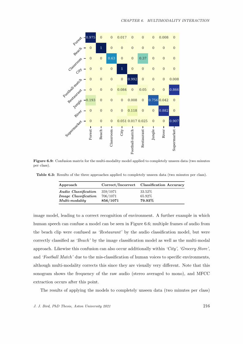
CHAPTER 6. MULTIMODALITY INTERACTION
Fore
st
Bea
ch
Cla
ssro
om City
Foot
ball-
mat
ch
Res
taur
ant
Jung
le
Riv
er
Supe
rmar
ket
Fores
t
Beach
Classro
om
City
Footb
all-m
atch
Restau
rant
Jung
le
River
Super
marke
t
0.975 0 0 0.017 0 0 0 0.008 0
0 1 0 0 0 0 0 0 0
0 0 0.63 0 0 0.37 0 0 0
0 0 0 1 0 0 0 0 0
0 0 0 0 0.992 0 0 0 0.008
0 0 0 0.084 0 0.05 0 0 0.866
0.193 0 0 0 0.008 0 0.756 0.042 0
0 0 0 0 0.118 0 0 0.882 0
0 0 0 0.051 0.017 0.025 0 0 0.907
Figure 6.9: Confusion matrix for the multi-modality model applied to completely unseen data (two minutesper class).
Table 6.3: Results of the three approaches applied to completely unseen data (two minutes per class).
Approach Correct/Incorrect Classification Accuracy
Audio Classification 359/1071 33.52%Image Classification 706/1071 65.92%Multi-modality 856/1071 79.93%
image model, leading to a correct recognition of environment. A further example in which
human speech can confuse a model can be seen in Figure 6.6; multiple frames of audio from
the beach clip were confused as ‘Restaurant’ by the audio classification model, but were
correctly classified as ‘Beach’ by the image classification model as well as the multi-modal
approach. Likewise this confusion can also occur additionally within ‘City’, ‘Grocery Store’,
and ‘Football Match’ due to the mis-classification of human voices to specific environments,
although multi-modality corrects this since they are visually very different. Note that this
sonogram shows the frequency of the raw audio (stereo averaged to mono), and MFCC
extraction occurs after this point.
The results of applying the models to completely unseen data (two minutes per class)
J. J. Bird, PhD Thesis, Aston University 2021 216
CHAPTER 6. MULTIMODALITY INTERACTION
can be seen in Table 6.3. It can be observed that audio classification of environments is
weak at 33.52%, which is outperformed by image classification at 65.92% accuracy. Both
approaches are outperformed by the multi-modality approach which scores 79.93% classi-
fication accuracy. The confusion matrix of the multi-modality model can be observed in
Figure 6.9; the main issue is caused by ‘Restaurant’ being confused as ‘Supermarket’, while
all other environments are classified strongly. On manual observation, the videos for both
classes in the unseen data both feature a large number of people with speech sound in the
background, this is possibly most similar to the supermarkets in the training dataset and
thus the model is confident that both of these instances belong to supermarket. This sug-
gests that the data could be more diversified in the future in order to feature more minute
details and thus improve the model’s ability for discerning between the two.
6.3 CNN transfer learning for Scene Classification
This section explores experiments which show that both fine-tune learning and cross-domain
sim-to-real transfer learning from virtual to real-world environments improve the starting
and final scene classification abilities of a computer vision model. The main finding is that
not only can a higher final classification accuracy be achieved, but strong classification
abilities prior to any training whatsoever are also encountered when transferring knowledge
from simulation to real-world data, showing useful domain knowledge transfer between the
datasets.
The possibility of transfer learning from simulated data to real-world application is
promising due to the scarcity of real-world labelled data being an issue encountered in
many applications of machine learning and artificial intelligence [428, 429, 430]. Based on
this, Fine-tune Learning and Transfer learning are often both considered to be viable so-
lutions to the issue of data scarcity in the scientific state-of-the-art via large-scale models
such as ImageNet and VGG16 for the former and methods such as rule and weight transfer
for the latter [431, 432, 433]. Here, both of these methods are performed in a pipeline for
scene classification, by fine-tuning a large-scale model and transferring knowledge between
rules learnt from simulation to real-world datasets.
The consumer-level quality of videogame technology has rapidly improved towards arguably
photo-realistic graphical quality through ray-traced lighting, high resolution photographic
J. J. Bird, PhD Thesis, Aston University 2021 217
CHAPTER 6. MULTIMODALITY INTERACTION
textures and Physically Based Rendering (PBR) to name several prominent techniques.
This then raises the question, since simulated environments are ever more realistic, is it
possible to transfer knowledge from them to real-world situations? Should this be possi-
ble, the problem of data scarcity would be mitigated, and also a more optimal process of
learning would become possible by introducing a starting point learned from simulation. If
this process provides a better starting point than, for example, a classical random weight
distribution, then fewer computational resources are required to learn about the real world
and also fewer labelled data points are required. In addition, if this process is improved
further, learning from real-world data may not actually be required at all.
This work explores 12 individual topology experiments to show that real-world classifi-
cation of relatively scarce data can be improved via pre-training said models on simulation
data from a high-quality videogame environment. The weights developed on simulation
data are applied as a starting point for the backpropagation learning of real-world data,
and it is found that both starting accuracy and asymptote (final ability) are often higher
when the model has been able to train on simulation data before considering real data.
The main scientific contributions of this work are threefold:
1. The formation of two datasets for a 6-class scene classification dataset, both artificial
simulation and real-world photographic data3.
2. 24 topology tuning experiments for best classification of the two datasets, 12 for
each of the datasets by 2, 4, 8...4096 interpretation neurons following the fine tuning
of a VGG16 CNN network (with interpretation and softmax layers removed). This
provides a baseline comparison for Transfer Learning as well as the pre-trained weights
to be used in the following experiment.
3. 12 transfer learning experiments of the weights trained on simulation data transferred
to networks with the task of classifying real-world data. The results are evidence
that transfer learning of useful domain knowledge is possible from the classification of
simulated environments to the classification of real-world photographic data, further
improving classification ability of real data.
3https://www.kaggle.com/birdy654/environment-recognition-simulation-to-reality
J. J. Bird, PhD Thesis, Aston University 2021 218
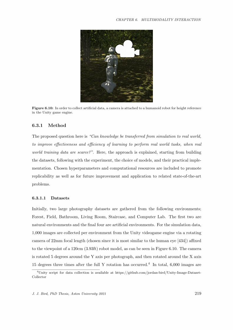
CHAPTER 6. MULTIMODALITY INTERACTION
Figure 6.10: In order to collect artificial data, a camera is attached to a humanoid robot for height referencein the Unity game engine.
6.3.1 Method
The proposed question here is “Can knowledge be transferred from simulation to real world,
to improve effectiveness and efficiency of learning to perform real world tasks, when real
world training data are scarce?”. Here, the approach is explained, starting from building
the datasets, following with the experiment, the choice of models, and their practical imple-
mentation. Chosen hyperparameters and computational resources are included to promote
replicability as well as for future improvement and application to related state-of-the-art
problems.
6.3.1.1 Datasets
Initially, two large photography datasets are gathered from the following environments;
Forest, Field, Bathroom, Living Room, Staircase, and Computer Lab. The first two are
natural environments and the final four are artificial environments. For the simulation data,
1,000 images are collected per environment from the Unity videogame engine via a rotating
camera of 22mm focal length (chosen since it is most similar to the human eye [434]) affixed
to the viewpoint of a 120cm (3.93ft) robot model, as can be seen in Figure 6.10. The camera
is rotated 5 degrees around the Y axis per photograph, and then rotated around the X axis
15 degrees three times after the full Y rotation has occurred.4 In total, 6,000 images are
4Unity script for data collection is available at https://github.com/jordan-bird/Unity-Image-Dataset-Collector
J. J. Bird, PhD Thesis, Aston University 2021 219
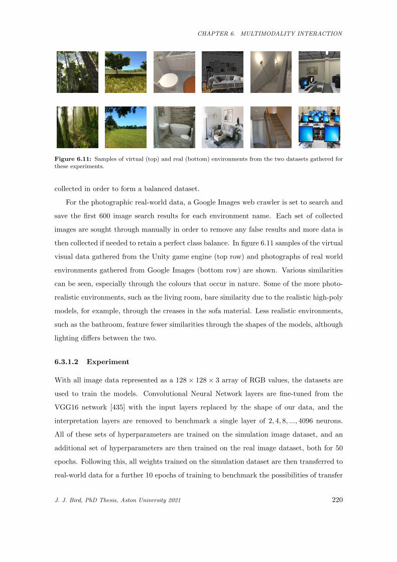
CHAPTER 6. MULTIMODALITY INTERACTION
Figure 6.11: Samples of virtual (top) and real (bottom) environments from the two datasets gathered forthese experiments.
collected in order to form a balanced dataset.
For the photographic real-world data, a Google Images web crawler is set to search and
save the first 600 image search results for each environment name. Each set of collected
images are sought through manually in order to remove any false results and more data is
then collected if needed to retain a perfect class balance. In figure 6.11 samples of the virtual
visual data gathered from the Unity game engine (top row) and photographs of real world
environments gathered from Google Images (bottom row) are shown. Various similarities
can be seen, especially through the colours that occur in nature. Some of the more photo-
realistic environments, such as the living room, bare similarity due to the realistic high-poly
models, for example, through the creases in the sofa material. Less realistic environments,
such as the bathroom, feature fewer similarities through the shapes of the models, although
lighting differs between the two.
6.3.1.2 Experiment
With all image data represented as a 128 × 128 × 3 array of RGB values, the datasets are
used to train the models. Convolutional Neural Network layers are fine-tuned from the
VGG16 network [435] with the input layers replaced by the shape of our data, and the
interpretation layers are removed to benchmark a single layer of 2, 4, 8, ..., 4096 neurons.
All of these sets of hyperparameters are trained on the simulation image dataset, and an
additional set of hyperparameters are then trained on the real image dataset, both for 50
epochs. Following this, all weights trained on the simulation dataset are then transferred to
real-world data for a further 10 epochs of training to benchmark the possibilities of transfer
J. J. Bird, PhD Thesis, Aston University 2021 220
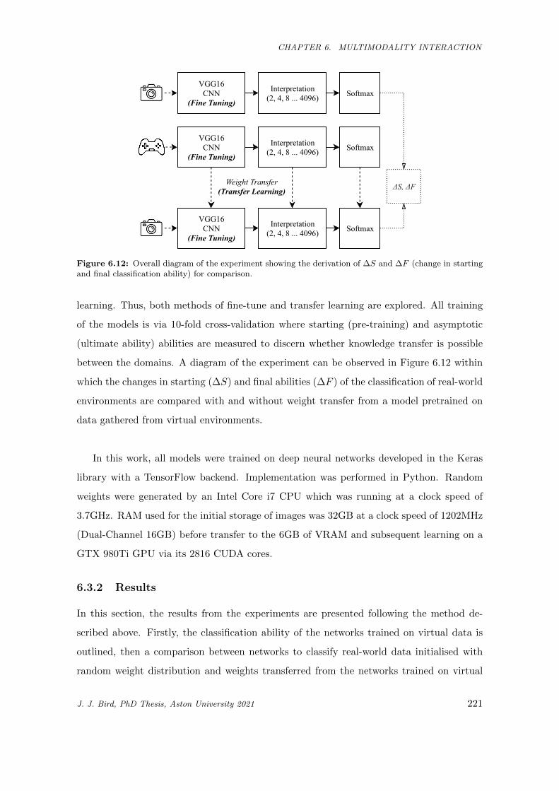
CHAPTER 6. MULTIMODALITY INTERACTION
VGG16CNN
(FineTuning)
VGG16CNN
(FineTuning)
Interpretation(2,4,8...4096)
Interpretation(2,4,8...4096)
Softmax
Softmax
VGG16CNN
(FineTuning)
Interpretation(2,4,8...4096) Softmax
WeightTransfer(TransferLearning) ΔS,ΔF
Figure 6.12: Overall diagram of the experiment showing the derivation of ∆S and ∆F (change in startingand final classification ability) for comparison.
learning. Thus, both methods of fine-tune and transfer learning are explored. All training
of the models is via 10-fold cross-validation where starting (pre-training) and asymptotic
(ultimate ability) abilities are measured to discern whether knowledge transfer is possible
between the domains. A diagram of the experiment can be observed in Figure 6.12 within
which the changes in starting (∆S) and final abilities (∆F ) of the classification of real-world
environments are compared with and without weight transfer from a model pretrained on
data gathered from virtual environments.
In this work, all models were trained on deep neural networks developed in the Keras
library with a TensorFlow backend. Implementation was performed in Python. Random
weights were generated by an Intel Core i7 CPU which was running at a clock speed of
3.7GHz. RAM used for the initial storage of images was 32GB at a clock speed of 1202MHz
(Dual-Channel 16GB) before transfer to the 6GB of VRAM and subsequent learning on a
GTX 980Ti GPU via its 2816 CUDA cores.
6.3.2 Results
In this section, the results from the experiments are presented following the method de-
scribed above. Firstly, the classification ability of the networks trained on virtual data is
outlined, then a comparison between networks to classify real-world data initialised with
random weight distribution and weights transferred from the networks trained on virtual
J. J. Bird, PhD Thesis, Aston University 2021 221
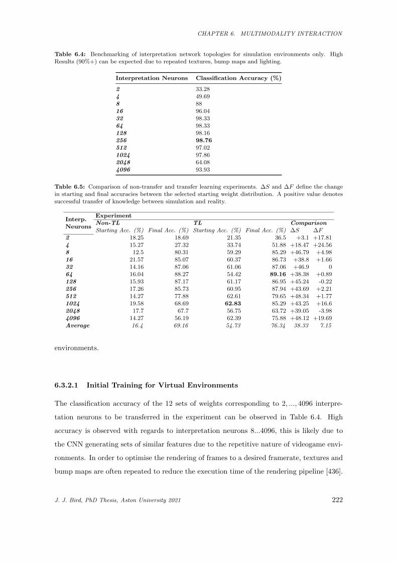
CHAPTER 6. MULTIMODALITY INTERACTION
Table 6.4: Benchmarking of interpretation network topologies for simulation environments only. HighResults (90%+) can be expected due to repeated textures, bump maps and lighting.
Interpretation Neurons Classification Accuracy (%)
2 33.284 49.698 8816 96.0432 98.3364 98.33128 98.16256 98.76512 97.021024 97.862048 64.084096 93.93
Table 6.5: Comparison of non-transfer and transfer learning experiments. ∆S and ∆F define the changein starting and final accuracies between the selected starting weight distribution. A positive value denotessuccessful transfer of knowledge between simulation and reality.
Interp.Neurons
ExperimentNon-TL TL ComparisonStarting Acc. (%) Final Acc. (%) Starting Acc. (%) Final Acc. (%) ∆S ∆F
2 18.25 18.69 21.35 36.5 +3.1 +17.814 15.27 27.32 33.74 51.88 +18.47 +24.568 12.5 80.31 59.29 85.29 +46.79 +4.9816 21.57 85.07 60.37 86.73 +38.8 +1.6632 14.16 87.06 61.06 87.06 +46.9 064 16.04 88.27 54.42 89.16 +38.38 +0.89128 15.93 87.17 61.17 86.95 +45.24 -0.22256 17.26 85.73 60.95 87.94 +43.69 +2.21512 14.27 77.88 62.61 79.65 +48.34 +1.771024 19.58 68.69 62.83 85.29 +43.25 +16.62048 17.7 67.7 56.75 63.72 +39.05 -3.984096 14.27 56.19 62.39 75.88 +48.12 +19.69Average 16.4 69.16 54.73 76.34 38.33 7.15
environments.
6.3.2.1 Initial Training for Virtual Environments
The classification accuracy of the 12 sets of weights corresponding to 2, ..., 4096 interpre-
tation neurons to be transferred in the experiment can be observed in Table 6.4. High
accuracy is observed with regards to interpretation neurons 8...4096, this is likely due to
the CNN generating sets of similar features due to the repetitive nature of videogame envi-
ronments. In order to optimise the rendering of frames to a desired framerate, textures and
bump maps are often repeated to reduce the execution time of the rendering pipeline [436].
J. J. Bird, PhD Thesis, Aston University 2021 222
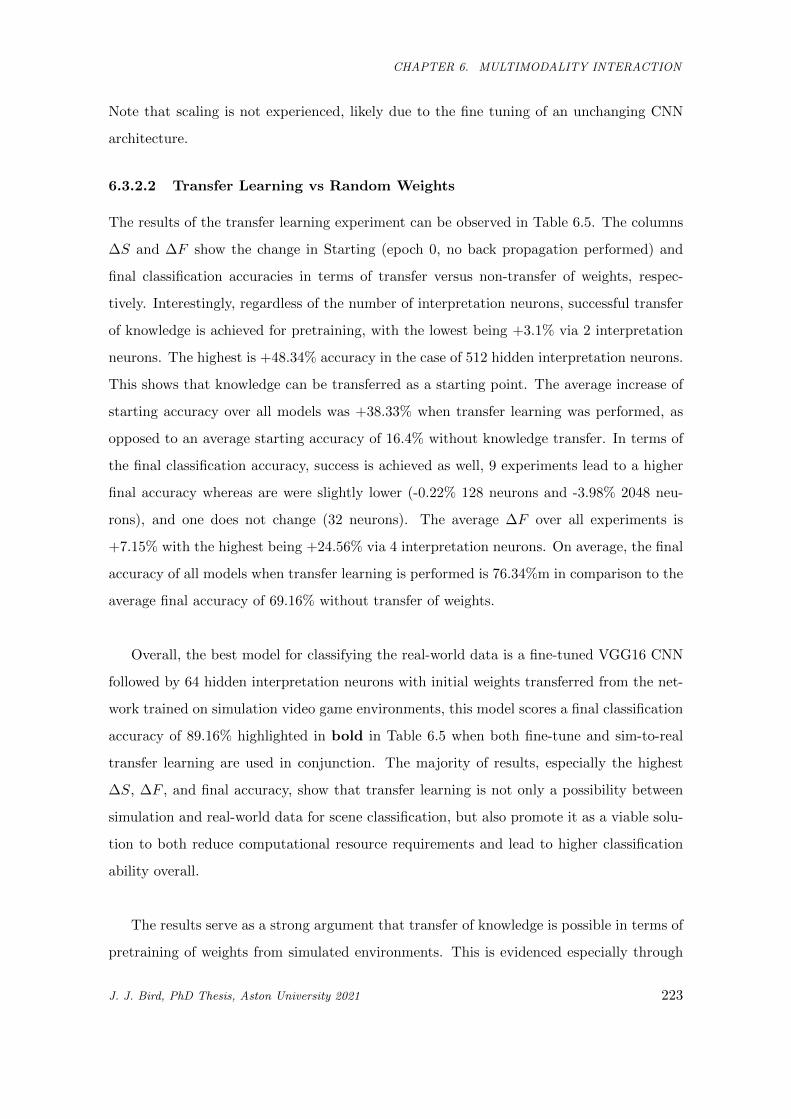
CHAPTER 6. MULTIMODALITY INTERACTION
Note that scaling is not experienced, likely due to the fine tuning of an unchanging CNN
architecture.
6.3.2.2 Transfer Learning vs Random Weights
The results of the transfer learning experiment can be observed in Table 6.5. The columns
∆S and ∆F show the change in Starting (epoch 0, no back propagation performed) and
final classification accuracies in terms of transfer versus non-transfer of weights, respec-
tively. Interestingly, regardless of the number of interpretation neurons, successful transfer
of knowledge is achieved for pretraining, with the lowest being +3.1% via 2 interpretation
neurons. The highest is +48.34% accuracy in the case of 512 hidden interpretation neurons.
This shows that knowledge can be transferred as a starting point. The average increase of
starting accuracy over all models was +38.33% when transfer learning was performed, as
opposed to an average starting accuracy of 16.4% without knowledge transfer. In terms of
the final classification accuracy, success is achieved as well, 9 experiments lead to a higher
final accuracy whereas are were slightly lower (-0.22% 128 neurons and -3.98% 2048 neu-
rons), and one does not change (32 neurons). The average ∆F over all experiments is
+7.15% with the highest being +24.56% via 4 interpretation neurons. On average, the final
accuracy of all models when transfer learning is performed is 76.34%m in comparison to the
average final accuracy of 69.16% without transfer of weights.
Overall, the best model for classifying the real-world data is a fine-tuned VGG16 CNN
followed by 64 hidden interpretation neurons with initial weights transferred from the net-
work trained on simulation video game environments, this model scores a final classification
accuracy of 89.16% highlighted in bold in Table 6.5 when both fine-tune and sim-to-real
transfer learning are used in conjunction. The majority of results, especially the highest
∆S, ∆F , and final accuracy, show that transfer learning is not only a possibility between
simulation and real-world data for scene classification, but also promote it as a viable solu-
tion to both reduce computational resource requirements and lead to higher classification
ability overall.
The results serve as a strong argument that transfer of knowledge is possible in terms of
pretraining of weights from simulated environments. This is evidenced especially through
J. J. Bird, PhD Thesis, Aston University 2021 223
CHAPTER 6. MULTIMODALITY INTERACTION
the initial ability of the transfer networks prior to any training for classification of the real
environments, but it is also shown through the best ultimate score achieved by a network
with initial weights transferred.
6.4 Sign Language Recognition via Late Fusion of Computer
Vision and Leap Motion
This sections shows that a late fusion approach to multi-modality in British Sign Lan-
guage recognition improves the overall ability of the model in comparison to the singular
approaches of RGB and Leap Motion data classification. Additionally, the work in this
section also discovers the possibility of transfer learning from the singular and multi-modal
models towards the improvement of a scarce dataset of American Sign Language via initial
weight distribution.
Sign language is the ability to converse mainly by the use of the hands, as well as in
some cases the body, face, and head. Recognition and understanding of Sign Language
is thus an entirely visuo-temporal process performed by human beings. In the United
Kingdom alone, there are 145,000 deaf adults and children who use British Sign Language
(BSL) [387]. Of those people, 15,000 report BSL as their main language of communica-
tion [437] which implies a difficulty of communication with those who cannot interpret the
language. Unfortunately, when another person cannot interpret sign language (of who are
the vast majority), a serious language barrier is present due to disability. In addition to
individuals who act as interpreters for those who can only converse in Sign Language, or
who only feel comfortable doing so, this work aims to improve autonomous classification
techniques towards dictation of Sign Language in real-time. The philosophy behind this
work is based on a simple argument, if a building were to have a ramp in addition to stairs
for easier access of the disabled, then why should a computer system not be present in order
to aid with those hard of hearing or deaf?. This work initially benchmarks two popular
methods of sign language recognition with an RGB camera and a Leap Motion 3D hand
tracking camera after gathering a large dataset of gestures. Following these initial exper-
iments, a multi-modality approach is then presented which fuses the two forms of data to
achieve better results for two main reasons; firstly, mistakes and anomalous data received
by either sensor has the chance to be mitigated by the other, and secondly, a deep neural
J. J. Bird, PhD Thesis, Aston University 2021 224
CHAPTER 6. MULTIMODALITY INTERACTION
network can learn to extract useful complimentary data from each sensor as well as the
standard approach of extracting information towards the class itself. The driving force be-
hind improving the ability of these two sensors is mainly cost, in that the solution presented
is of extremely minimal cost and with further improvement beyond the 18 gestures explored
in this study, could easily be implemented within public places such as restaurants, schools,
and libraries etc. to improve the lives of disabled individuals and enable communication
with those they otherwise could not communicate with.
In this work, the approaches of single modality learning and classification are compared
to multi-modality late fusion. The main scientific contributions presented by this work are
as follows:
1. Collection of a large BSL dataset from five subjects and a medium-sized ASL dataset
from two subjects5.
2. Tuning of classification models for the RGB camera (processing layer prior to output),
Leap Motion Classification (evolutionary topology search), and multi-modality late
fusion of the two via concatenation to a neural layer. Findings show that multi-
modality is the strongest approach for BSL classification compared to the two single-
modality inputs as well as state of the art statistical learning techniques.
3. Transfer learning from BSL to improve ASL classification. Findings show that weight
transfer to the multi-modality model is the strongest approach for ASL classification.
6.4.1 Method
Within this section, the proposed approaches for late fusion experiments are described.
The experiments that this section mainly refers to can be observed in Figure 6.13 which
outlines the image classification, Leap Motion classification, and multi-modality late fusion
networks. The camera is used to record an image, and features are extracted via the VGG16
CNN and MLP. The Leap motion is used to record a numerical vector representing the 3D
hand features previously described, which serves as input to an evolutionarily-optimised
deep MLP. Given that the data is recorded synchronously, that is, the image from the
camera and the numerical vector from the Leap Motion are captured at the same moment
5The dataset is publicly available at https://www.kaggle.com/birdy654/sign-language-recognition-leap-motion
J. J. Bird, PhD Thesis, Aston University 2021 225
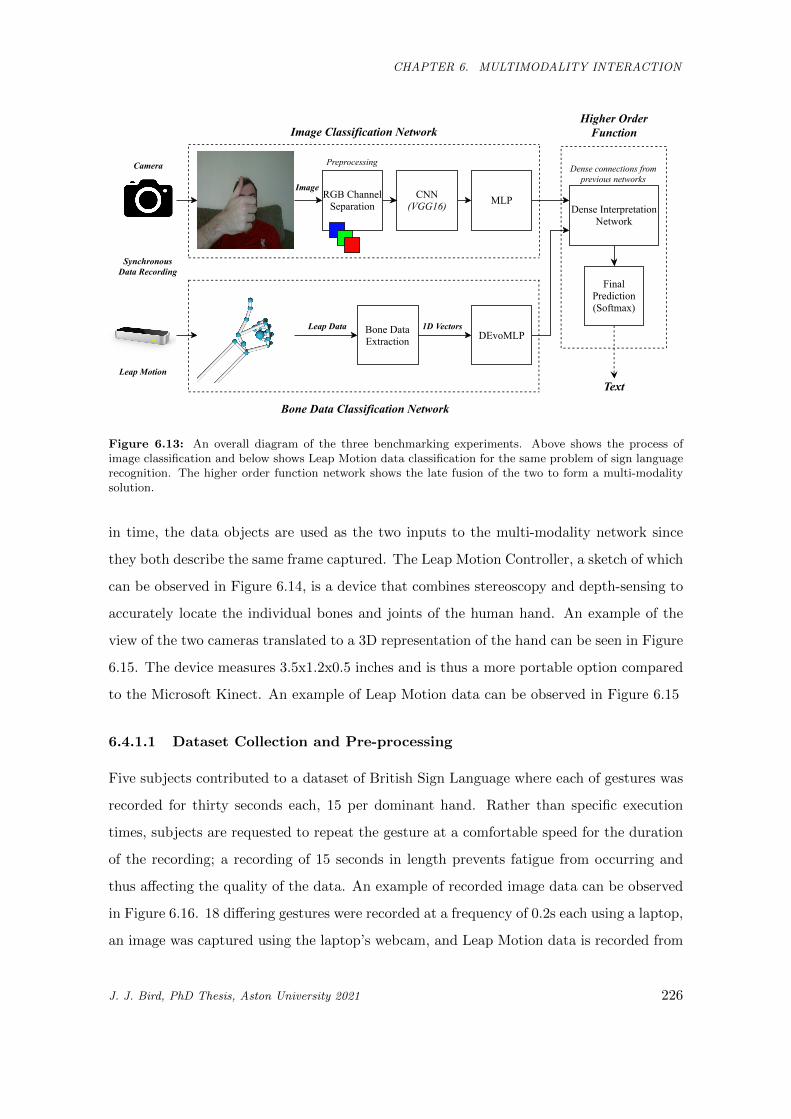
CHAPTER 6. MULTIMODALITY INTERACTION
CNN(VGG16)
DEvoMLP
MLPDenseInterpretation
Network
FinalPrediction(Softmax)
LeapData
Image
ImageClassificationNetwork
BoneDataClassificationNetwork
Text
BoneDataExtraction
HigherOrderFunction
RGBChannelSeparation
PreprocessingDenseconnectionsfrompreviousnetworks
1DVectors
LeapMotion
Camera
SynchronousDataRecording
Figure 6.13: An overall diagram of the three benchmarking experiments. Above shows the process ofimage classification and below shows Leap Motion data classification for the same problem of sign languagerecognition. The higher order function network shows the late fusion of the two to form a multi-modalitysolution.
in time, the data objects are used as the two inputs to the multi-modality network since
they both describe the same frame captured. The Leap Motion Controller, a sketch of which
can be observed in Figure 6.14, is a device that combines stereoscopy and depth-sensing to
accurately locate the individual bones and joints of the human hand. An example of the
view of the two cameras translated to a 3D representation of the hand can be seen in Figure
6.15. The device measures 3.5x1.2x0.5 inches and is thus a more portable option compared
to the Microsoft Kinect. An example of Leap Motion data can be observed in Figure 6.15
6.4.1.1 Dataset Collection and Pre-processing
Five subjects contributed to a dataset of British Sign Language where each of gestures was
recorded for thirty seconds each, 15 per dominant hand. Rather than specific execution
times, subjects are requested to repeat the gesture at a comfortable speed for the duration
of the recording; a recording of 15 seconds in length prevents fatigue from occurring and
thus affecting the quality of the data. An example of recorded image data can be observed
in Figure 6.16. 18 differing gestures were recorded at a frequency of 0.2s each using a laptop,
an image was captured using the laptop’s webcam, and Leap Motion data is recorded from
J. J. Bird, PhD Thesis, Aston University 2021 226
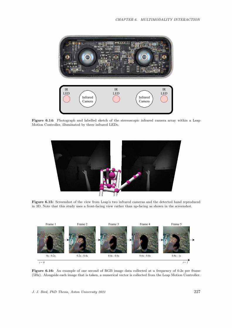
CHAPTER 6. MULTIMODALITY INTERACTION
InfraredCamera
InfraredCamera
IRLED
IRLED
IRLED
Figure 6.14: Photograph and labelled sketch of the stereoscopic infrared camera array within a LeapMotion Controller, illuminated by three infrared LEDs.
Figure 6.15: Screenshot of the view from Leap’s two infrared cameras and the detected hand reproducedin 3D. Note that this study uses a front-facing view rather than up-facing as shown in the screenshot.
0s-0.2s 0.2s-0.4s 0.4s-0.6s 0.6s-0.8s 0.8s-1s
Frame1 Frame2 Frame3 Frame4 Frame5
t=0 t=1
Figure 6.16: An example of one second of RGB image data collected at a frequency of 0.2s per frame(5Hz). Alongside each image that is taken, a numerical vector is collected from the Leap Motion Controller.
J. J. Bird, PhD Thesis, Aston University 2021 227
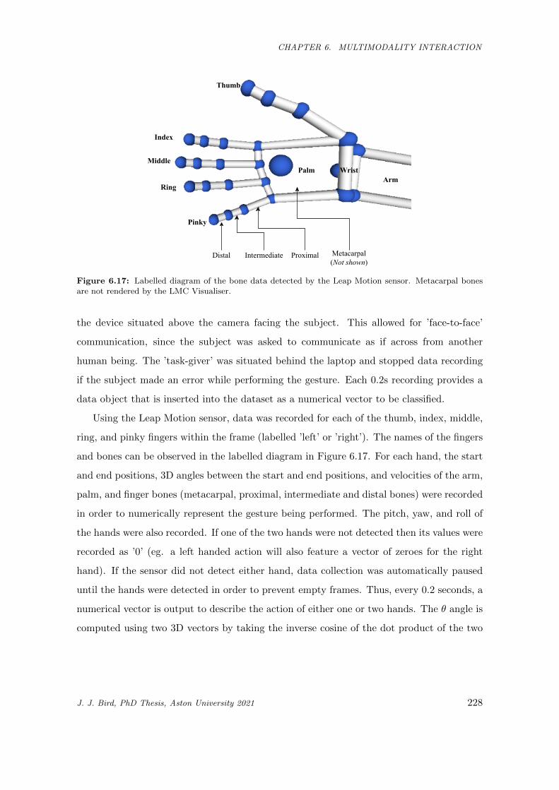
CHAPTER 6. MULTIMODALITY INTERACTION
Distal Intermediate Proximal Metacarpal(Notshown)
Thumb
Index
Middle
Ring
Pinky
PalmArm
Wrist
Figure 6.17: Labelled diagram of the bone data detected by the Leap Motion sensor. Metacarpal bonesare not rendered by the LMC Visualiser.
the device situated above the camera facing the subject. This allowed for ’face-to-face’
communication, since the subject was asked to communicate as if across from another
human being. The ’task-giver’ was situated behind the laptop and stopped data recording
if the subject made an error while performing the gesture. Each 0.2s recording provides a
data object that is inserted into the dataset as a numerical vector to be classified.
Using the Leap Motion sensor, data was recorded for each of the thumb, index, middle,
ring, and pinky fingers within the frame (labelled ’left’ or ’right’). The names of the fingers
and bones can be observed in the labelled diagram in Figure 6.17. For each hand, the start
and end positions, 3D angles between the start and end positions, and velocities of the arm,
palm, and finger bones (metacarpal, proximal, intermediate and distal bones) were recorded
in order to numerically represent the gesture being performed. The pitch, yaw, and roll of
the hands were also recorded. If one of the two hands were not detected then its values were
recorded as ’0’ (eg. a left handed action will also feature a vector of zeroes for the right
hand). If the sensor did not detect either hand, data collection was automatically paused
until the hands were detected in order to prevent empty frames. Thus, every 0.2 seconds, a
numerical vector is output to describe the action of either one or two hands. The θ angle is
computed using two 3D vectors by taking the inverse cosine of the dot product of the two
J. J. Bird, PhD Thesis, Aston University 2021 228

CHAPTER 6. MULTIMODALITY INTERACTION
vectors divided by the magnitudes of each vector as shown below:
θ = arccos
(ab
| a || b |
), (6.1)
where | a | and | b | are:
| a |=√ax2 + ay2 + az2
| b |=√bx
2 + by2 + bz
2,
(6.2)
Regarding the x, y, and z co-ordinates of each point in space. The start and end points of
each bone in the hand from the LMC are treated as the two points.
The following is a summary of each feature collected from the hierarchy of arm to finger
joint:
• For each arm: Start position of the arm (X, Y, and Z), End position of the arm (X,
Y, and Z), 3D angle between start and end positions of the arm, Velocity of the arm
(X, Y, and Z)
• For each elbow: Position of the elbow (X, Y, and Z)
• For each wrist: Position of the wrist (X, Y, and Z)
• For each palm: Pitch, Yaw, Roll, 3D angle of the palm, Position of the palm (X, Y,
and Z), Velocity of the palm (X, Y, and Z), Normal of the palm (X, Y, and Z)
• For each finger: Direction of the finger (X, Y, and Z), Position of the finger (X, Y,
and Z), Velocity of the finger (X, Y, and Z)
• For each finger joint: Start position of the joint (X, Y, and Z), End position of the
joint (X, Y, and Z), 3D angle of the joint, Direction of the finger (X, Y, and Z),
Position of the joint (X, Y, and Z), Velocity of the joint (X, Y, and Z)
Each feature was pre-processed via a minmax scaler between 0 (min) and 1 (max):
Feat = Featstd(max−min) +min where Featstd = ( Feat−FeatminFeatmax−Featmin
). Thus, each feature
value is reduced to a value between 0 and 1. This was performed since it was observed that
non-processed feature values caused issues for the model and often resulted in classification
accuracy scores of only approximately 4%, showing a failure to generalise. The 18 British
J. J. Bird, PhD Thesis, Aston University 2021 229
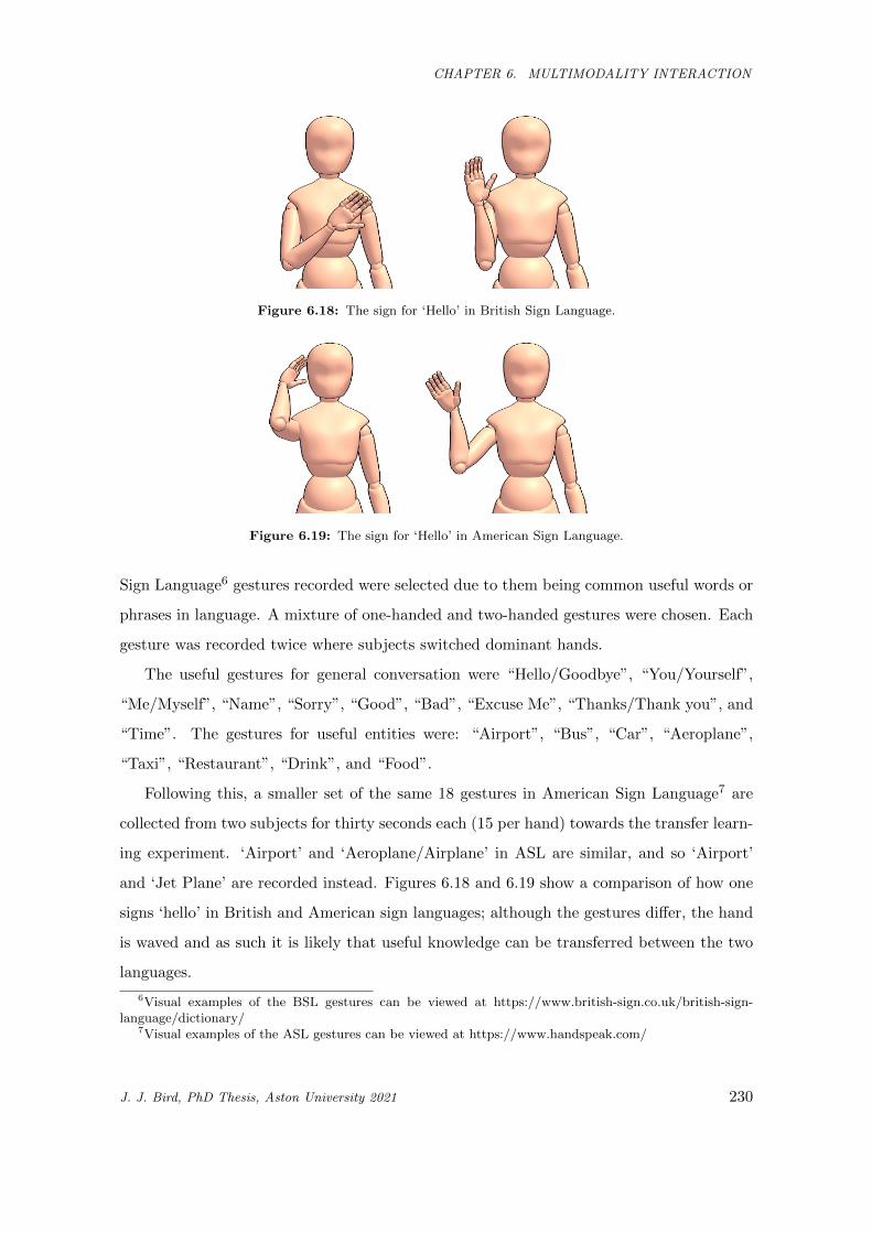
CHAPTER 6. MULTIMODALITY INTERACTION
Figure 6.18: The sign for ‘Hello’ in British Sign Language.
Figure 6.19: The sign for ‘Hello’ in American Sign Language.
Sign Language6 gestures recorded were selected due to them being common useful words or
phrases in language. A mixture of one-handed and two-handed gestures were chosen. Each
gesture was recorded twice where subjects switched dominant hands.
The useful gestures for general conversation were “Hello/Goodbye”, “You/Yourself”,
“Me/Myself”, “Name”, “Sorry”, “Good”, “Bad”, “Excuse Me”, “Thanks/Thank you”, and
“Time”. The gestures for useful entities were: “Airport”, “Bus”, “Car”, “Aeroplane”,
“Taxi”, “Restaurant”, “Drink”, and “Food”.
Following this, a smaller set of the same 18 gestures in American Sign Language7 are
collected from two subjects for thirty seconds each (15 per hand) towards the transfer learn-
ing experiment. ‘Airport’ and ‘Aeroplane/Airplane’ in ASL are similar, and so ‘Airport’
and ‘Jet Plane’ are recorded instead. Figures 6.18 and 6.19 show a comparison of how one
signs ‘hello’ in British and American sign languages; although the gestures differ, the hand
is waved and as such it is likely that useful knowledge can be transferred between the two
languages.
6Visual examples of the BSL gestures can be viewed at https://www.british-sign.co.uk/british-sign-language/dictionary/
7Visual examples of the ASL gestures can be viewed at https://www.handspeak.com/
J. J. Bird, PhD Thesis, Aston University 2021 230
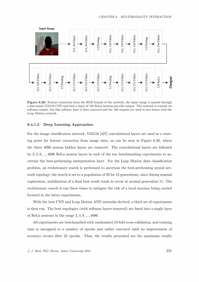
CHAPTER 6. MULTIMODALITY INTERACTION
3x3,64Filters
3x3,64Filters
1/2Pooling
3x3,128Filters
3x3,128Filters
3x3,128Filters
1/2Pooling
3x3,256Filters
3x3,256Filters
3x3,256Filters
1/2Pooling
3x3,512Filters
3x3,512Filters
3x3,512Filters
1/2Pooling
3x3,512Filters
3x3,512Filters
3x3,512Filters
128ReLu
InputImage
Output
Figure 6.20: Feature extraction from the RGB branch of the network, the input image is passed througha fine-tuned VGG16 CNN and then a layer of 128 ReLu neurons provide output. The network is trained viasoftmax output, but this softmax layer is later removed and the 128 outputs are used in late fusion with theLeap Motion network.
6.4.1.2 Deep Learning Approaches
For the image classification network, VGG16 [427] convolutional layers are used as a start-
ing point for feature extraction from image data, as can be seen in Figure 6.20, where
the three 4096 neuron hidden layers are removed. The convolutional layers are followed
by 2, 4, 8, ..., 4096 ReLu neuron layers in each of the ten benchmarking experiments to as-
certain the best-performing interpretation layer. For the Leap Motion data classification
problem, an evolutionary search is performed to ascertain the best-performing neural net-
work topology; the search is set to a population of 20 for 15 generations, since during manual
exploration, stabilisation of a final best result tends to occur at around generation 11. The
evolutionary search is run three times to mitigate the risk of a local maxima being carried
forward in the latter experiments.
With the best CNN and Leap Motion ANN networks derived, a third set of experiments
is then run. The best topologies (with softmax layers removed) are fused into a single layer
of ReLu neurons in the range 2, 4, 8, ..., 4096.
All experiments are benchmarked with randomised 10-fold cross-validation, and training
time is uncapped to a number of epochs and rather executed until no improvement of
accuracy occurs after 25 epochs. Thus, the results presented are the maximum results
J. J. Bird, PhD Thesis, Aston University 2021 231
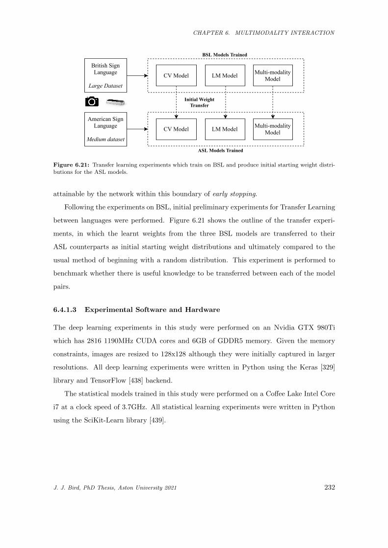
CHAPTER 6. MULTIMODALITY INTERACTION
BritishSignLanguage
LargeDataset
AmericanSignLanguage
Mediumdataset
CVModel LMModel Multi-modalityModel
CVModel LMModel Multi-modalityModel
InitialWeightTransfer
BSLModelsTrained
ASLModelsTrained
Figure 6.21: Transfer learning experiments which train on BSL and produce initial starting weight distri-butions for the ASL models.
attainable by the network within this boundary of early stopping.
Following the experiments on BSL, initial preliminary experiments for Transfer Learning
between languages were performed. Figure 6.21 shows the outline of the transfer experi-
ments, in which the learnt weights from the three BSL models are transferred to their
ASL counterparts as initial starting weight distributions and ultimately compared to the
usual method of beginning with a random distribution. This experiment is performed to
benchmark whether there is useful knowledge to be transferred between each of the model
pairs.
6.4.1.3 Experimental Software and Hardware
The deep learning experiments in this study were performed on an Nvidia GTX 980Ti
which has 2816 1190MHz CUDA cores and 6GB of GDDR5 memory. Given the memory
constraints, images are resized to 128x128 although they were initially captured in larger
resolutions. All deep learning experiments were written in Python using the Keras [329]
library and TensorFlow [438] backend.
The statistical models trained in this study were performed on a Coffee Lake Intel Core
i7 at a clock speed of 3.7GHz. All statistical learning experiments were written in Python
using the SciKit-Learn library [439].
J. J. Bird, PhD Thesis, Aston University 2021 232
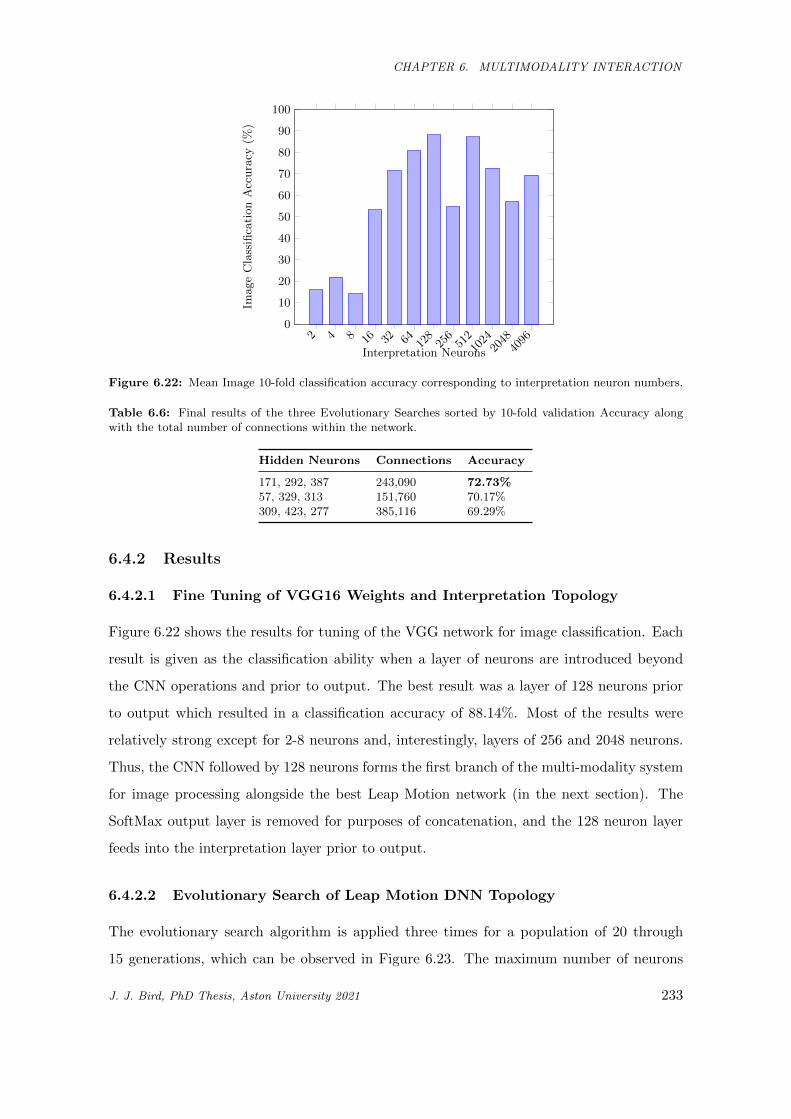
CHAPTER 6. MULTIMODALITY INTERACTION
2 4 8 16 32 64 128
256
51210
2420
4840
960
10
20
30
40
50
60
70
80
90
100
Interpretation Neurons
Image
Cla
ssifi
cati
on
Acc
ura
cy(%
)
Figure 6.22: Mean Image 10-fold classification accuracy corresponding to interpretation neuron numbers.
Table 6.6: Final results of the three Evolutionary Searches sorted by 10-fold validation Accuracy alongwith the total number of connections within the network.
Hidden Neurons Connections Accuracy
171, 292, 387 243,090 72.73%57, 329, 313 151,760 70.17%309, 423, 277 385,116 69.29%
6.4.2 Results
6.4.2.1 Fine Tuning of VGG16 Weights and Interpretation Topology
Figure 6.22 shows the results for tuning of the VGG network for image classification. Each
result is given as the classification ability when a layer of neurons are introduced beyond
the CNN operations and prior to output. The best result was a layer of 128 neurons prior
to output which resulted in a classification accuracy of 88.14%. Most of the results were
relatively strong except for 2-8 neurons and, interestingly, layers of 256 and 2048 neurons.
Thus, the CNN followed by 128 neurons forms the first branch of the multi-modality system
for image processing alongside the best Leap Motion network (in the next section). The
SoftMax output layer is removed for purposes of concatenation, and the 128 neuron layer
feeds into the interpretation layer prior to output.
6.4.2.2 Evolutionary Search of Leap Motion DNN Topology
The evolutionary search algorithm is applied three times for a population of 20 through
15 generations, which can be observed in Figure 6.23. The maximum number of neurons
J. J. Bird, PhD Thesis, Aston University 2021 233
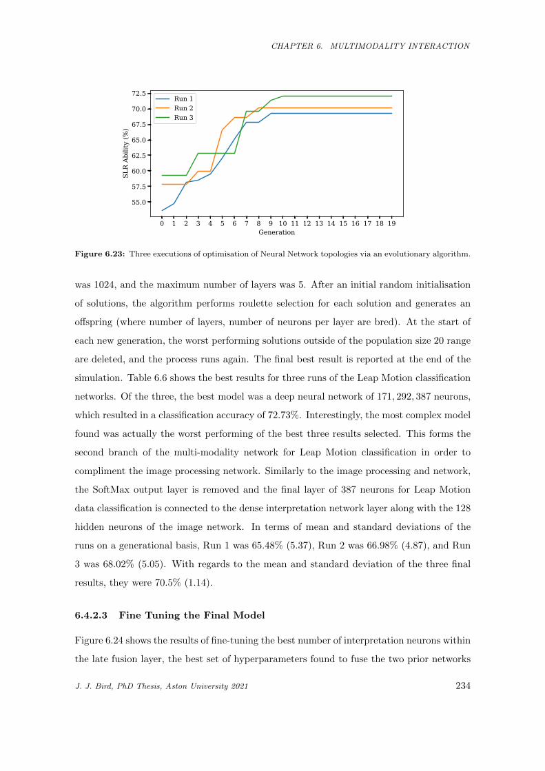
CHAPTER 6. MULTIMODALITY INTERACTION
0 1 2 3 4 5 6 7 8 9 10 11 12 13 14 15 16 17 18 19Generation
55.0
57.5
60.0
62.5
65.0
67.5
70.0
72.5
SLR
Abi
lity
(%)
Run 1Run 2Run 3
Figure 6.23: Three executions of optimisation of Neural Network topologies via an evolutionary algorithm.
was 1024, and the maximum number of layers was 5. After an initial random initialisation
of solutions, the algorithm performs roulette selection for each solution and generates an
offspring (where number of layers, number of neurons per layer are bred). At the start of
each new generation, the worst performing solutions outside of the population size 20 range
are deleted, and the process runs again. The final best result is reported at the end of the
simulation. Table 6.6 shows the best results for three runs of the Leap Motion classification
networks. Of the three, the best model was a deep neural network of 171, 292, 387 neurons,
which resulted in a classification accuracy of 72.73%. Interestingly, the most complex model
found was actually the worst performing of the best three results selected. This forms the
second branch of the multi-modality network for Leap Motion classification in order to
compliment the image processing network. Similarly to the image processing and network,
the SoftMax output layer is removed and the final layer of 387 neurons for Leap Motion
data classification is connected to the dense interpretation network layer along with the 128
hidden neurons of the image network. In terms of mean and standard deviations of the
runs on a generational basis, Run 1 was 65.48% (5.37), Run 2 was 66.98% (4.87), and Run
3 was 68.02% (5.05). With regards to the mean and standard deviation of the three final
results, they were 70.5% (1.14).
6.4.2.3 Fine Tuning the Final Model
Figure 6.24 shows the results of fine-tuning the best number of interpretation neurons within
the late fusion layer, the best set of hyperparameters found to fuse the two prior networks
J. J. Bird, PhD Thesis, Aston University 2021 234
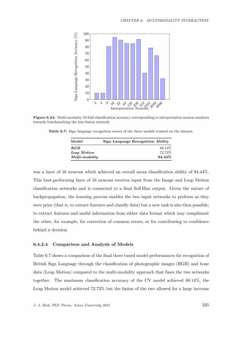
CHAPTER 6. MULTIMODALITY INTERACTION
2 4 8 16 32 64 128
256
51210
2420
4840
960
10
20
30
40
50
60
70
80
90
100
Interpretation Neurons
Sig
nL
an
gu
age
Rec
ogn
itio
nA
ccu
racy
(%)
Figure 6.24: Multi-modality 10-fold classification accuracy corresponding to interpretation neuron numberstowards benchmarking the late-fusion network.
Table 6.7: Sign language recognition scores of the three models trained on the dataset.
Model Sign Language Recognition Ability
RGB 88.14%Leap Motion 72.73%Multi-modality 94.44%
was a layer of 16 neurons which achieved an overall mean classification ability of 94.44%.
This best-performing layer of 16 neurons receives input from the Image and Leap Motion
classification networks and is connected to a final SoftMax output. Given the nature of
backpropagation, the learning process enables the two input networks to perform as they
were prior (that is, to extract features and classify data) but a new task is also then possible;
to extract features and useful information from either data format which may compliment
the other, for example, for correction of common errors, or for contributing to confidence
behind a decision.
6.4.2.4 Comparison and Analysis of Models
Table 6.7 shows a comparison of the final three tuned model performances for recognition of
British Sign Language through the classification of photographic images (RGB) and bone
data (Leap Motion) compared to the multi-modality approach that fuses the two networks
together. The maximum classification accuracy of the CV model achieved 88.14%, the
Leap Motion model achieved 72.73% but the fusion of the two allowed for a large increase
J. J. Bird, PhD Thesis, Aston University 2021 235
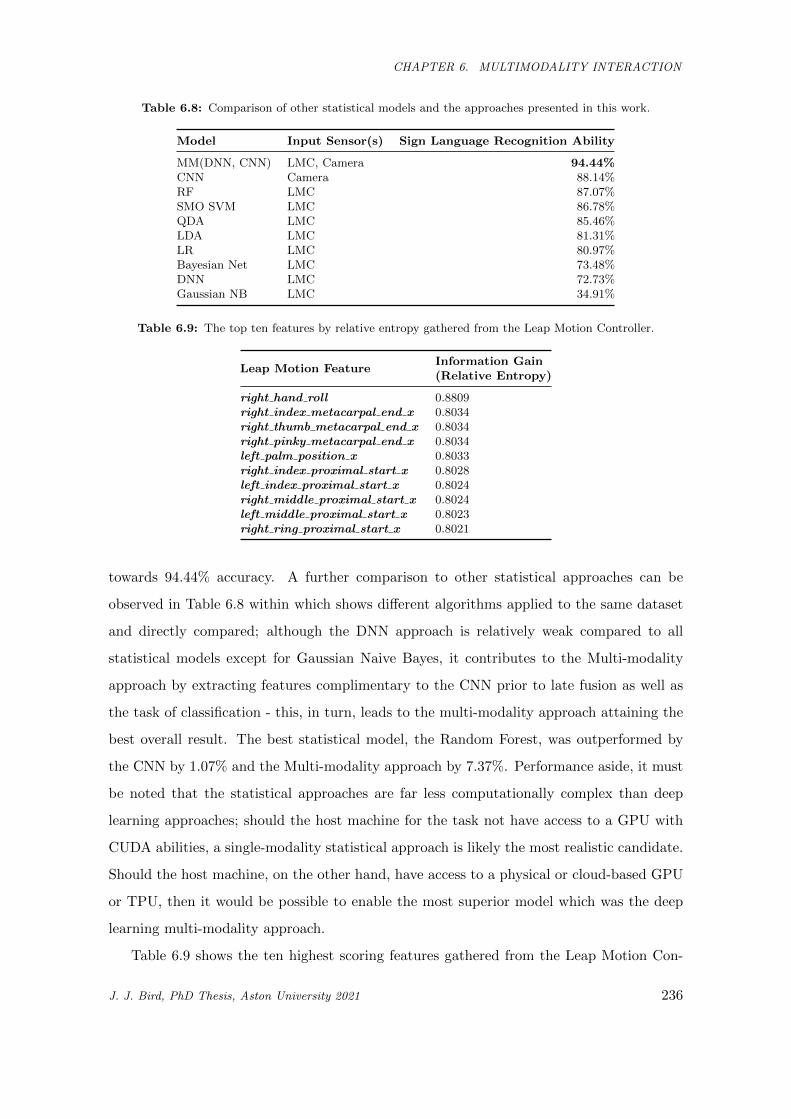
CHAPTER 6. MULTIMODALITY INTERACTION
Table 6.8: Comparison of other statistical models and the approaches presented in this work.
Model Input Sensor(s) Sign Language Recognition Ability
MM(DNN, CNN) LMC, Camera 94.44%CNN Camera 88.14%RF LMC 87.07%SMO SVM LMC 86.78%QDA LMC 85.46%LDA LMC 81.31%LR LMC 80.97%Bayesian Net LMC 73.48%DNN LMC 72.73%Gaussian NB LMC 34.91%
Table 6.9: The top ten features by relative entropy gathered from the Leap Motion Controller.
Leap Motion FeatureInformation Gain(Relative Entropy)
right hand roll 0.8809right index metacarpal end x 0.8034right thumb metacarpal end x 0.8034right pinky metacarpal end x 0.8034left palm position x 0.8033right index proximal start x 0.8028left index proximal start x 0.8024right middle proximal start x 0.8024left middle proximal start x 0.8023right ring proximal start x 0.8021
towards 94.44% accuracy. A further comparison to other statistical approaches can be
observed in Table 6.8 within which shows different algorithms applied to the same dataset
and directly compared; although the DNN approach is relatively weak compared to all
statistical models except for Gaussian Naive Bayes, it contributes to the Multi-modality
approach by extracting features complimentary to the CNN prior to late fusion as well as
the task of classification - this, in turn, leads to the multi-modality approach attaining the
best overall result. The best statistical model, the Random Forest, was outperformed by
the CNN by 1.07% and the Multi-modality approach by 7.37%. Performance aside, it must
be noted that the statistical approaches are far less computationally complex than deep
learning approaches; should the host machine for the task not have access to a GPU with
CUDA abilities, a single-modality statistical approach is likely the most realistic candidate.
Should the host machine, on the other hand, have access to a physical or cloud-based GPU
or TPU, then it would be possible to enable the most superior model which was the deep
learning multi-modality approach.
Table 6.9 shows the ten highest scoring features gathered from the Leap Motion Con-
J. J. Bird, PhD Thesis, Aston University 2021 236
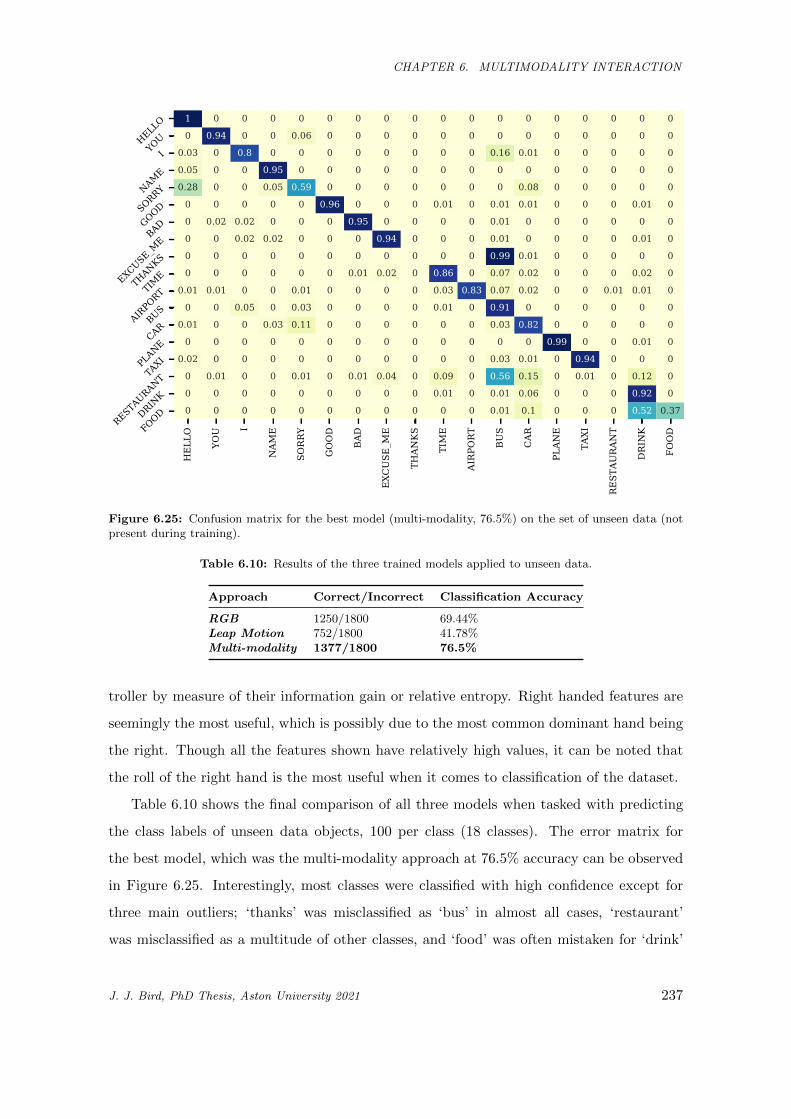
CHAPTER 6. MULTIMODALITY INTERACTION
HELL
O
YOU I
NAM
E
SORRY
GOOD
BAD
EXC
USE
_ME
THAN
KS
TIME
AIRPO
RT
BUS
CAR
PLAN
E
TAXI
REST
AURAN
T
DRIN
K
FOOD
HELLO
YOUI
NAME
SORRY
GOOD
BAD
EXCUSE_ME
THANKS
TIME
AIRPORT
BUS
CAR
PLANE
TAXI
RESTAURANT
DRINK
FOOD
1 0 0 0 0 0 0 0 0 0 0 0 0 0 0 0 0 0
0 0.94 0 0 0.06 0 0 0 0 0 0 0 0 0 0 0 0 0
0.03 0 0.8 0 0 0 0 0 0 0 0 0.16 0.01 0 0 0 0 0
0.05 0 0 0.95 0 0 0 0 0 0 0 0 0 0 0 0 0 0
0.28 0 0 0.05 0.59 0 0 0 0 0 0 0 0.08 0 0 0 0 0
0 0 0 0 0 0.96 0 0 0 0.01 0 0.01 0.01 0 0 0 0.01 0
0 0.02 0.02 0 0 0 0.95 0 0 0 0 0.01 0 0 0 0 0 0
0 0 0.02 0.02 0 0 0 0.94 0 0 0 0.01 0 0 0 0 0.01 0
0 0 0 0 0 0 0 0 0 0 0 0.99 0.01 0 0 0 0 0
0 0 0 0 0 0 0.01 0.02 0 0.86 0 0.07 0.02 0 0 0 0.02 0
0.01 0.01 0 0 0.01 0 0 0 0 0.03 0.83 0.07 0.02 0 0 0.01 0.01 0
0 0 0.05 0 0.03 0 0 0 0 0.01 0 0.91 0 0 0 0 0 0
0.01 0 0 0.03 0.11 0 0 0 0 0 0 0.03 0.82 0 0 0 0 0
0 0 0 0 0 0 0 0 0 0 0 0 0 0.99 0 0 0.01 0
0.02 0 0 0 0 0 0 0 0 0 0 0.03 0.01 0 0.94 0 0 0
0 0.01 0 0 0.01 0 0.01 0.04 0 0.09 0 0.56 0.15 0 0.01 0 0.12 0
0 0 0 0 0 0 0 0 0 0.01 0 0.01 0.06 0 0 0 0.92 0
0 0 0 0 0 0 0 0 0 0 0 0.01 0.1 0 0 0 0.52 0.37
Figure 6.25: Confusion matrix for the best model (multi-modality, 76.5%) on the set of unseen data (notpresent during training).
Table 6.10: Results of the three trained models applied to unseen data.
Approach Correct/Incorrect Classification Accuracy
RGB 1250/1800 69.44%Leap Motion 752/1800 41.78%Multi-modality 1377/1800 76.5%
troller by measure of their information gain or relative entropy. Right handed features are
seemingly the most useful, which is possibly due to the most common dominant hand being
the right. Though all the features shown have relatively high values, it can be noted that
the roll of the right hand is the most useful when it comes to classification of the dataset.
Table 6.10 shows the final comparison of all three models when tasked with predicting
the class labels of unseen data objects, 100 per class (18 classes). The error matrix for
the best model, which was the multi-modality approach at 76.5% accuracy can be observed
in Figure 6.25. Interestingly, most classes were classified with high confidence except for
three main outliers; ‘thanks’ was misclassified as ‘bus’ in almost all cases, ‘restaurant’
was misclassified as a multitude of other classes, and ‘food’ was often mistaken for ‘drink’
J. J. Bird, PhD Thesis, Aston University 2021 237
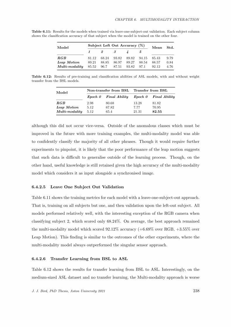
CHAPTER 6. MULTIMODALITY INTERACTION
Table 6.11: Results for the models when trained via leave-one-subject-out validation. Each subject columnshows the classification accuracy of that subject when the model is trained on the other four.
ModelSubject Left Out Accuracy (%)
Mean Std.1 2 3 4 5
RGB 81.12 68.24 93.82 89.82 94.15 85.43 9.79Leap Motion 89.21 88.85 86.97 89.27 88.54 88.57 0.84Multi-modality 85.52 96.7 87.51 93.82 97.1 92.12 4.76
Table 6.12: Results of pre-training and classification abilities of ASL models, with and without weighttransfer from the BSL models.
ModelNon-transfer from BSL Transfer from BSL
Epoch 0 Final Ability Epoch 0 Final Ability
RGB 2.98 80.68 13.28 81.82Leap Motion 5.12 67.82 7.77 70.95Multi-modality 5.12 65.4 21.31 82.55
although this did not occur vice-versa. Outside of the anomalous classes which must be
improved in the future with more training examples, the multi-modality model was able
to confidently classify the majority of all other phrases. Though it would require further
experiments to pinpoint, it is likely that the poor performance of the leap motion suggests
that such data is difficult to generalise outside of the learning process. Though, on the
other hand, useful knowledge is still retained given the high accuracy of the multi-modality
model which considers it as input alongside a synchronised image.
6.4.2.5 Leave One Subject Out Validation
Table 6.11 shows the training metrics for each model with a leave-one-subject-out approach.
That is, training on all subjects but one, and then validation upon the left-out subject. All
models performed relatively well, with the interesting exception of the RGB camera when
classifying subject 2, which scored only 68.24%. On average, the best approach remained
the multi-modality model which scored 92.12% accuracy (+6.69% over RGB, +3.55% over
Leap Motion). This finding is similar to the outcomes of the other experiments, where the
multi-modality model always outperformed the singular sensor approach.
6.4.2.6 Transfer Learning from BSL to ASL
Table 6.12 shows the results for transfer learning from BSL to ASL. Interestingly, on the
medium-sized ASL dataset and no transfer learning, the Multi-modality approach is worse
J. J. Bird, PhD Thesis, Aston University 2021 238
CHAPTER 6. MULTIMODALITY INTERACTION
than both the Computer Vision and Leap Motion models singularly. This, and considering
that the best model overall for ASL classification was the Multi-modality model with weight
transfer from the BSL model, suggests that data scarcity poses an issue for multi-modality
models for this problem.
The results show that transfer learning improves the abilities of the Leap Motion and
Multi-modality classification approaches to sign language recognition. With this in mind,
availability of trained weights may be useful to improve the classification of other datasets
regardless of whether or not they are in the same sign language. Overall, the best model
for ASL classification was the multi-modality model when weights are transferred from the
BSL model. This approach scored 82.55% classification ability on the ASL dataset. The
results suggest that useful knowledge can be transferred between sign languages for image
classification, Leap Motion classification, and late fusion of the two towards multi-modality
classification.
Though future work is needed to further explore the transfer learning hypotheses, the
results in these initial experiments suggest the possibility of success when transferring knowl-
edge between models and ultimately improving their recognition performances.
6.5 Summary and Conclusion
This Chapter focused on the exploration of abilities for the HRI framework, focusing on
multimodal learning. Firstly, Section 6.2 presented three models for scene recognition. A
vision model through fine-tuned VGG16 weights for classification of images of environments,
and a deep neural network for classification of audio of environments. Following these,
the two models were then concatenated in synchronicity towards a multi-modal approach,
which outperformed the two original approaches through the gained ability of detection of
anomalous data through consideration of the outputs of both models. The tertiary neural
network for late fusion was compared and found to be superior to Naive Bayes, Random
Forest, and Support Vector Machine classifiers. Since audio classification is a relatively
easy task, it should be implemented where available to improve environmental recognition
tasks. Future work is suggested in order to take this successful preliminary experiment and
improve it further. These experiments focused on the context of autonomous machines,
and thus consumer hardware capability was taken into account through temporal awareness
J. J. Bird, PhD Thesis, Aston University 2021 239
CHAPTER 6. MULTIMODALITY INTERACTION
implemented within the feature extraction process rather than within the learning process
itself to save on resources during this stage. In the future, better results could be gained
from attempting to enable a neural network to learn temporal awareness in recurrence. This
could then be compared to the results found within this work. Since the model was found
to be effective on the complex problem posed through the dataset, future experiments could
concern other publicly available datasets to give a comparison with other state-of-the-art
methods. With the available hardware, evolutionary selection of network topology was
only possible with the audio classifier, in the future, given more resources, this algorithm
could be applied to both the vision and interpretation models to achieve a better set of
hyperparameters beyond the tuning performed in this study. Applications of the model
due to success should also be tested in real-world applications, for example, recent research
has show that autonomous environment recognition is useful in the automatic application
of scene settings for hearing aids [440]. Future works could also consider the optimisation
of the frame segmentation process itself as well as exploration of the possibility of multiple
image inputs per task. Additionally, since late fusion is promising due to the results found in
Section 6.2, applications to video classification tasks could be considered through a similar
multi-modal feature extraction and classification process; a more complex task would also
likely lead to a larger number of failure cases for the approach and thus provide clear errors
which would aid in further optimisation to overcome them and as such improve the model.
In addition to multimodal input, another improvement on scene recognition for the
framework was also explored in the context of transferring knowledge from a virtual en-
vironment to real data. The experiments and results presented in Section 6.3 showed the
success of transfer learning from virtual environments to another task taking place in reality.
From the results observed in this study, there are two main areas of future work which are
important to follow. Firstly, it is proposed to further improve the artificial learning pipeline.
Models were trained for 50 epochs for each of the interpretation layers to be benchmarked.
In future, the possibility of deeper networks with more than one hidden interpretation layer
and other combinations of the hyperparameters could be explored. The training time of the
random weight networks was relatively limited at 50 epochs and even further limited for
transfer learning at 10 epochs, although this was by design and due to the computational
resources available. Future work could concern deeper interpretation networks as well as
increased training time. In this study, hyperparameters such as the activation and learning
J. J. Bird, PhD Thesis, Aston University 2021 240
CHAPTER 6. MULTIMODALITY INTERACTION
rate optimisation algorithm were arbitrarily chosen, therefore, in the future, these could
be explored in a further combinatorial optimisation experiment. Secondly, simulation to
real transfer learning could also be attempted in various fields in order to benchmark the
ability of this method for other real-world applications. For example, autonomous cars
and drones training in a virtual environment for real-world applications. The next step for
benchmarking could be to compare the ability of this method to state-of-the-art methods on
publicly available datasets, should more computational resources be available, similarly to
the related works featured in the literature review [215, 216, 201]. A noticeable set of high
abilities were encountered for the sole classification of virtual data, as expected, due to the
optimisation processes of recycling objects and repeating textures found within videogame
environments. Of the 12 networks trained with and without transfer learning, a pattern of
knowledge transfer was observed; with all starting accuracies being substantially higher than
a random weight distribution, and, most importantly, a best classification ability of 89.16%
was achieved when knowledge was initially transferred from the virtual environments. These
results provide a strong argument for the application of both fine-tune and transfer learning
for autonomous scene recognition. The former was achieved through the tuning of VGG16
Convolutional Neural Networks, and the latter was achieved by transferring weights from a
network trained on simulation data from videogames and applied to a real-world situation.
Transfer learning leads to both the reduction of resource requirements for said problems,
and the achievement of a higher classification ability overall when pre-training has been
performed on simulated data. As future directions, further improvement of the learning
pipeline benchmarked in Section 6.3 together with exploration on other complex real-world
problems faced by autonomous machines are suggested.
Section 6.4 presented multiple experiments for the singular sensor and multi-modality
approaches to British and American Sign Language. The results from the experiments
suggest that a multi-modality approach outperforms the two singular sensors during both
training and for classification of unseen data. Section 6.4 also presented a preliminary
Transfer Learning experiment from the large BSL dataset to a medium-sized ASL dataset,
where the best model for classification of ASL was found to be the multi-modality model
when weights are transferred from the BSL model. All network topologies in this section
that were trained, compared, and ultimately fused together towards multi-modality were
benchmarked and studied for the first time. Accurate classification of Sign Language,
J. J. Bird, PhD Thesis, Aston University 2021 241
CHAPTER 6. MULTIMODALITY INTERACTION
especially unseen data, enables the ability to perform the task autonomously and thus
provide a digital method to the interpretation of non-spoken language within a situation
where interpretation is required but unavailable. To fully realise this possibility, future work
is needed. The hypotheses in the experiments were argued through a set of 18 common
gestures in both British and American Sign Languages. In future, additional classes are
required to allow for interpretation of conversations rather than the symbolic communication
enabled by this study. In addition, since multi-modality classification proved effective,
further tuning of hyperparameters could enable better results, and other methods of data
fusion could be explored in addition to the late fusion approach that was selected. Transfer
learning could be explored with other forms of non-spoken language such as, for example,
Indo-Pakistani SL which has an ethnologue of 1.5 million people and Brazilian SL with
an ethnologue of 200,000 people. The aim of Section 6.4 was to explore the viability and
ability of multi-modality in Sign Language Recognition by comparing Leap Motion and
RGB classification with their late-fusion counterparts. In addition, the 0.2s data collection
frame poses a limitation to these studies, and as such, further work could be performed to
derive the best window length for data collection. A cause for concern that was noted in
Section 6.4 was the reduction of ability when unseen data is considered, which is often the
case in machine learning exercises. Such experiments and metrics (ability on unseen dataset,
per-class abilities) are rarely performed and noted in the State of the Art works within sign
language recognition. Since the main goal of autonomous sign language recognition is to
provide a users with a system which can aid those who otherwise may not have access
to a method of translation and communication, it is important to consider how such a
system would perform when using trained models to classify data that were not present in
the training set. That is, real-time classification of data during usage of the system and
subsequently the trained classification models. Section 6.4 found high training results for
both modalities and multi-modality, deriving abilities that are competitive when indirectly
compared to the state of the art works in the field. When the best performing 94.44%
classification ability model (multi-modality) was applied to unseen data, it achieved 76.5%
accuracy mainly due to confusion within the ‘thanks’ and ‘restaurant’ classes. Likewise,
the RGB model reduced from 88.14% to 69.44% and the Leap Motion model reduced from
72.73% to 41.78% when comparing training accuracy and unseen data classification ability.
Future work is needed to enable the models a better ability to generalise towards real-time
J. J. Bird, PhD Thesis, Aston University 2021 242
CHAPTER 6. MULTIMODALITY INTERACTION
classification abilities that closely resemble their abilities observed during training.
In this chapter, three new multimodality capabilities were experimented with and bench-
marked for the Human-Robot Interaction framework. To conclude, these were: the improve-
ment of scene recognition through sound and images (Section 6.2) as well as transferring
useful knowledge from simulated environments to real environments (Section 6.3). Then,
finally, experiments that argued towards multimodality being more robust than individual
classification based on the inputs of a Leap Motion sensor and images (Section 6.4). With
the goals of this thesis in mind, the first set of scene recognition experiments and the sign
language experiments provide two abilities for the system which are again improved by
the multimodality approach as shown by the comparisons in each. The second set of scene
recognition experiments showed that scene recognition ability could be improved by transfer
learning from virtual, simulated environments, and thus, it can improve the robot’s ability
to perform this task.
J. J. Bird, PhD Thesis, Aston University 2021 243
CHAPTER 7. HUMAN-ROBOT INTERACTION FRAMEWORK
Chapter 7
Integration into a Human-Robot
Interaction Framework
7.1 Introduction
Following on the scientific contributions across the various fields presented in Chapters 4,
5, and 6, the main focus of the thesis is the unification of these technologies into a HRI
framework.
Firstly, the possibility of encapsulating these technologies within an abstract wrapper
of social interaction is explored. Then, an integrated HRI framework is presented to unify
the contributions of a singular system. Finally, the use cases of the framework are explored
where selected technologies from the framework are used in unison to achieve a certain
specific goal, through chatbot-like command recognition of activities such as classification
of brain activity, sentiment analysis of a given text, sign language recognition, and scene
recognition.
7.2 Chatbot Interface: Human Data Augmentation with T5
and Transformer Ensemble
In this section of the thesis, the Chatbot Interaction with Artificial Intelligence (CI-AI)
pipeline is presented as an approach to the training of deep learning chatbots for task
recognition. The intelligent system augments human-sourced data via artificial paraphras-
J. J. Bird, PhD Thesis, Aston University 2021 244
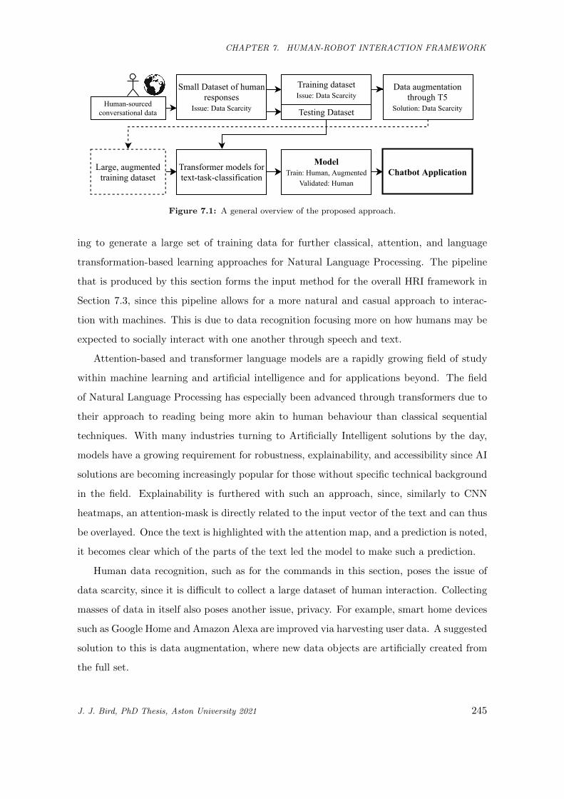
CHAPTER 7. HUMAN-ROBOT INTERACTION FRAMEWORK
SmallDatasetofhumanresponses
Issue:DataScarcityHuman-sourcedconversationaldata TestingDataset
TrainingdatasetIssue:DataScarcity
DataaugmentationthroughT5
Solution:DataScarcity
Transformermodelsfortext-task-classification ChatbotApplication
ModelTrain:Human,Augmented
Validated:Human
Large,augmentedtrainingdataset
Figure 7.1: A general overview of the proposed approach.
ing to generate a large set of training data for further classical, attention, and language
transformation-based learning approaches for Natural Language Processing. The pipeline
that is produced by this section forms the input method for the overall HRI framework in
Section 7.3, since this pipeline allows for a more natural and casual approach to interac-
tion with machines. This is due to data recognition focusing more on how humans may be
expected to socially interact with one another through speech and text.
Attention-based and transformer language models are a rapidly growing field of study
within machine learning and artificial intelligence and for applications beyond. The field
of Natural Language Processing has especially been advanced through transformers due to
their approach to reading being more akin to human behaviour than classical sequential
techniques. With many industries turning to Artificially Intelligent solutions by the day,
models have a growing requirement for robustness, explainability, and accessibility since AI
solutions are becoming increasingly popular for those without specific technical background
in the field. Explainability is furthered with such an approach, since, similarly to CNN
heatmaps, an attention-mask is directly related to the input vector of the text and can thus
be overlayed. Once the text is highlighted with the attention map, and a prediction is noted,
it becomes clear which of the parts of the text led the model to make such a prediction.
Human data recognition, such as for the commands in this section, poses the issue of
data scarcity, since it is difficult to collect a large dataset of human interaction. Collecting
masses of data in itself also poses another issue, privacy. For example, smart home devices
such as Google Home and Amazon Alexa are improved via harvesting user data. A suggested
solution to this is data augmentation, where new data objects are artificially created from
the full set.
J. J. Bird, PhD Thesis, Aston University 2021 245
CHAPTER 7. HUMAN-ROBOT INTERACTION FRAMEWORK
This study brings together the concepts of task recognition, language transformers, and
data augmentation to form a pipeline of Chatbot Interaction with Artificial Intelligence (CI-
AI). A general overview of the approach can be observed in Figure 7.1. As an alternative to
writing code and managing data, complex machine learning tasks such as conversational AI,
sentiment analysis, scene recognition, brainwave classification and sign language recognition
among others are given accessibility through an interface of natural, social interaction via
both verbal and non-verbal communication. That is, for example, a spoken command
of “can we have a conversation?” or a sign language command of “can-we-talk” would
command the system to launch a conversational AI program.
Since these experiments are performed in English, and there are many English speakers
across the world, the system thus needs to be accessible by many people with differing
backgrounds, and therefore must have the ability to generalise by being exposed to a large
amount of training data. Last, but by no means least, the system needs to be explainable;
for example, if a human were to utter the phrase, “Feeling sad today. Can you cheer me
up with a joke?”, which features within that phrase lead to a correct classification and
command to the chatbot to tell a joke? Where does the model focus within the given text
to correctly predict and fulfil the human’s request?
The scientific contributions of the work in this Section are as follows:
1. The collection of a 7-class command-to-task (with relation to the HRI framework’s
abilities implemented within the previous chapters) dataset from multiple human be-
ings from around the world, which produced a total of 483 examples.
2. Augmentation of the human data with a transformer-based paraphrasing model which
results in a final training dataset of 13,090 labelled data objects.
3. Benchmarking of 7 State-of-the-Art transformer-based classification approaches for
text-to-task commands. Each model is trained on the real training data and validation
data. Each model is also trained on the real training data plus the paraphrased
augmented data and validation data. It is observed that all 7 models are improved
significantly through data augmentation.
4. Analysis of the models in terms of the features within data which were given the most
attention, that is, which words or phrases were given specific focus. This is performed
for the errors in order to discern and discuss why the confusion occurred.
J. J. Bird, PhD Thesis, Aston University 2021 246
CHAPTER 7. HUMAN-ROBOT INTERACTION FRAMEWORK
5. It is observed that attention given to specific parts of sentences bare some general
similarities to human reading comprehension. This is found when the system considers
human phrases that were not present during training or validation through the analysis
of the most important features (words and phrases).
7.2.1 Method
The work in this section focuses on exploring a method to improve intent recognition.
As discussed during literature review, Google’s DialogFlow matches a user input (text,
speech-to-text, etc.) to an intent and then performs a task based on this intent. Given that
examples of intents would require data of a social nature from human beings to be collected,
and such tasks are often hampered by data scarcity, what can be done to alleviate this open
issue in the field? The solution explored here is a data augmentation method to use a general
knowledge of the English language to rephrase intents, forming them in alternative ways
to provide synthetic data which can be used during the training of a chatbot model. The
main aim of this section is to enable accessibility to previous studies, and in particular the
machine learning models derived throughout them. Accessibility is presented in the form of
social interaction, where a user requests to use a system in particular via natural language
and the task is derived and performed. The seven commands are mainly based on prior
work within this thesis, “have a conversation” and “tell me a joke” tasks are introduced for
further complexity since they both bare similarity in the sense of more casual interaction:
• Scene Recognition (Section 6.2) - The participant requests a scene recognition algo-
rithm to be instantiated, a camera and microphone are activated for multi-modality
classification.
• EEG Classification (Section 5.3) - The participant requests an EEG classification
algorithm to be instantiated and begins streaming data from a MUSE EEG headband,
there are two algorithms1:
– EEG Mental State Classification - Classification of whether the participant is
concentrating, relaxed, or neutral.
– EEG Emotional State Classification - Classification of emotional valence, posi-
tive, negative, or neutral.1Note that the two EEG tasks are similar, and discerning between the two provides a difficult problem
J. J. Bird, PhD Thesis, Aston University 2021 247
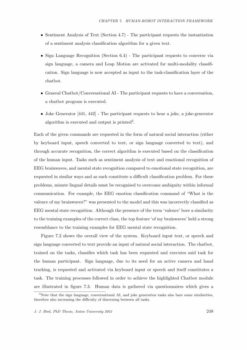
CHAPTER 7. HUMAN-ROBOT INTERACTION FRAMEWORK
• Sentiment Analysis of Text (Section 4.7) - The participant requests the instantiation
of a sentiment analysis classification algorithm for a given text.
• Sign Language Recognition (Section 6.4) - The participant requests to converse via
sign language, a camera and Leap Motion are activated for multi-modality classifi-
cation. Sign language is now accepted as input to the task-classification layer of the
chatbot.
• General Chatbot/Conversational AI - The participant requests to have a conversation,
a chatbot program is executed.
• Joke Generator [441, 442] - The participant requests to hear a joke, a joke-generator
algorithm is executed and output is printed2.
Each of the given commands are requested in the form of natural social interaction (either
by keyboard input, speech converted to text, or sign language converted to text), and
through accurate recognition, the correct algorithm is executed based on the classification
of the human input. Tasks such as sentiment analysis of text and emotional recognition of
EEG brainwaves, and mental state recognition compared to emotional state recognition, are
requested in similar ways and as such constitute a difficult classification problem. For these
problems, minute lingual details must be recognised to overcome ambiguity within informal
communication. For example, the EEG emotion classification command of “What is the
valence of my brainwaves?” was presented to the model and this was incorrectly classified as
EEG mental state recognition. Although the presence of the term ‘valence’ bore a similarity
to the training examples of the correct class, the top feature ‘of my brainwaves’ held a strong
resemblance to the training examples for EEG mental state recognition.
Figure 7.2 shows the overall view of the system. Keyboard input text, or speech and
sign language converted to text provide an input of natural social interaction. The chatbot,
trained on the tasks, classifies which task has been requested and executes said task for
the human participant. Sign language, due to its need for an active camera and hand
tracking, is requested and activated via keyboard input or speech and itself constitutes a
task. The training processes followed in order to achieve the highlighted Chatbot module
are illustrated in figure 7.3. Human data is gathered via questionnaires which gives a
2Note that the sign language, conversational AI, and joke generation tasks also bare some similarities,therefore also increasing the difficulty of discerning between all tasks.
J. J. Bird, PhD Thesis, Aston University 2021 248
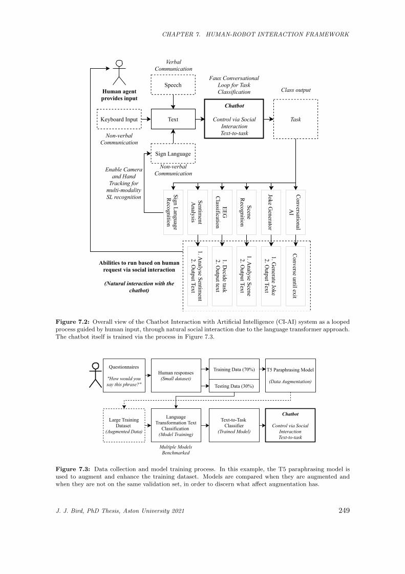
CHAPTER 7. HUMAN-ROBOT INTERACTION FRAMEWORK
Chatbot
ControlviaSocialInteractionText-to-task
Text
Speech
SignLanguage
KeyboardInput
Conversational
AI
SignLanguageRecognition
JokeGenerator
EEGClassification
Task
SceneRecognition
Converseuntilexit
1.GenerateJoke
2.OutputText
1.Decidetask
2.Outputtext
Abilitiestorunbasedonhumanrequestviasocialinteraction
(Naturalinteractionwiththechatbot)
1.AnalyseScene
2.OutputText
VerbalCommunication
Non-verbalCommunication
Non-verbalCommunication
Sentiment
Analysis
1.AnalyseSentim
ent2.O
utputText
FauxConversationalLoopforTaskClassification Classoutput
EnableCameraandHandTrackingformulti-modalitySLrecognition
Humanagentprovidesinput
Figure 7.2: Overall view of the Chatbot Interaction with Artificial Intelligence (CI-AI) system as a loopedprocess guided by human input, through natural social interaction due to the language transformer approach.The chatbot itself is trained via the process in Figure 7.3.
Humanresponses(Smalldataset)
Questionnaires
"Howwouldyousaythisphrase?" TestingData(30%)
TrainingData(70%) T5ParaphrasingModel
(DataAugmentation)
LanguageTransformationText
Classification(ModelTraining)
Chatbot
ControlviaSocialInteractionText-to-task
Text-to-TaskClassifier
(TrainedModel)
MultipleModelsBenchmarked
LargeTrainingDataset
(AugmentedData)
Figure 7.3: Data collection and model training process. In this example, the T5 paraphrasing model isused to augment and enhance the training dataset. Models are compared when they are augmented andwhen they are not on the same validation set, in order to discern what affect augmentation has.
J. J. Bird, PhD Thesis, Aston University 2021 249
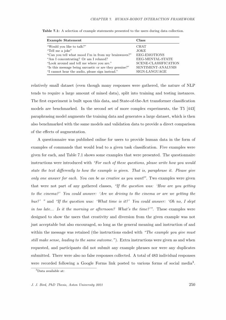
CHAPTER 7. HUMAN-ROBOT INTERACTION FRAMEWORK
Table 7.1: A selection of example statements presented to the users during data collection.
Example Statement Class
“Would you like to talk?” CHAT“Tell me a joke” JOKE“Can you tell what mood I’m in from my brainwaves?” EEG-EMOTIONS“Am I concentrating? Or am I relaxed? EEG-MENTAL-STATE“Look around and tell me where you are.” SCENE-CLASSIFICATION“Is this message being sarcastic or are they genuine?” SENTIMENT-ANALYSIS“I cannot hear the audio, please sign instead.” SIGN-LANGUAGE
relatively small dataset (even though many responses were gathered, the nature of NLP
tends to require a large amount of mined data), split into training and testing instances.
The first experiment is built upon this data, and State-of-the-Art transformer classification
models are benchmarked. In the second set of more complex experiments, the T5 [443]
paraphrasing model augments the training data and generates a large dataset, which is then
also benchmarked with the same models and validation data to provide a direct comparison
of the effects of augmentation.
A questionnaire was published online for users to provide human data in the form of
examples of commands that would lead to a given task classification. Five examples were
given for each, and Table 7.1 shows some examples that were presented. The questionnaire
instructions were introduced with “For each of these questions, please write how you would
state the text differently to how the example is given. That is, paraphrase it. Please give
only one answer for each. You can be as creative as you want!”. Two examples were given
that were not part of any gathered classes, “If the question was: ‘How are you getting
to the cinema?’ You could answer: ‘Are we driving to the cinema or are we getting the
bus?’ ” and “If the question was: ‘What time is it?’ You could answer: ‘Oh no, I slept
in too late... Is it the morning or afternoon? What’s the time?’”. These examples were
designed to show the users that creativity and diversion from the given example was not
just acceptable but also encouraged, so long as the general meaning and instruction of and
within the message was retained (the instructions ended with “The example you give must
still make sense, leading to the same outcome.”). Extra instructions were given as and when
requested, and participants did not submit any example phrases nor were any duplicates
submitted. There were also no false responses collected. A total of 483 individual responses
were recorded following a Google Forms link posted to various forms of social media3.
3Data available at:
J. J. Bird, PhD Thesis, Aston University 2021 250
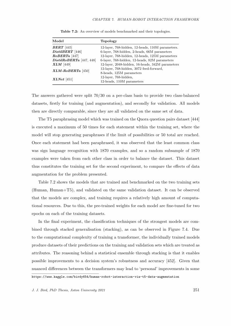
CHAPTER 7. HUMAN-ROBOT INTERACTION FRAMEWORK
Table 7.2: An overview of models benchmarked and their topologies.
Model Topology
BERT [445] 12-layer, 768-hidden, 12-heads, 110M parameters.DistilBERT [446] 6-layer, 768-hidden, 2-heads, 66M parametersRoBERTa [447] 12-layer, 768-hidden, 12-heads, 125M parametersDistilRoBERTa [447, 448] 6-layer, 768-hidden, 12-heads, 82M parametersXLM [449] 12-layer, 2048-hidden, 16-heads, 342M parameters
XLM-RoBERTa [450]12-layer, 768-hidden, 3072 feed-forward,8-heads, 125M parameters
XLNet [451]12-layer, 768-hidden,12-heads, 110M parameters
The answers gathered were split 70/30 on a per-class basis to provide two class-balanced
datasets, firstly for training (and augmentation), and secondly for validation. All models
then are directly comparable, since they are all validated on the same set of data.
The T5 paraphrasing model which was trained on the Quora question pairs dataset [444]
is executed a maximum of 50 times for each statement within the training set, where the
model will stop generating paraphrases if the limit of possibilities or 50 total are reached.
Once each statement had been paraphrased, it was observed that the least common class
was sign language recognition with 1870 examples, and so a random subsample of 1870
examples were taken from each other class in order to balance the dataset. This dataset
thus constitutes the training set for the second experiment, to compare the effects of data
augmentation for the problem presented.
Table 7.2 shows the models that are trained and benchmarked on the two training sets
(Human, Human+T5), and validated on the same validation dataset. It can be observed
that the models are complex, and training requires a relatively high amount of computa-
tional resources. Due to this, the pre-trained weights for each model are fine-tuned for two
epochs on each of the training datasets.
In the final experiment, the classification techniques of the strongest models are com-
bined through stacked generalisation (stacking), as can be observed in Figure 7.4. Due
to the computational complexity of training a transformer, the individually trained models
produce datasets of their predictions on the training and validation sets which are treated as
attributes. The reasoning behind a statistical ensemble through stacking is that it enables
possible improvements to a decision system’s robustness and accuracy [452]. Given that
nuanced differences between the transformers may lead to ‘personal’ improvements in some
https://www.kaggle.com/birdy654/human-robot-interaction-via-t5-data-augmentation
J. J. Bird, PhD Thesis, Aston University 2021 251
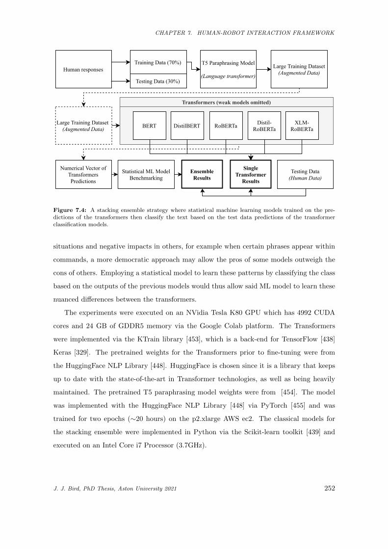
CHAPTER 7. HUMAN-ROBOT INTERACTION FRAMEWORK
BERT DistilBERT XLM-RoBERTa
Distil-RoBERTaRoBERTa
NumericalVectorofTransformersPredictions
Humanresponses
TestingData(30%)
TrainingData(70%) T5ParaphrasingModel
(Languagetransformer)
LargeTrainingDataset(AugmentedData)
LargeTrainingDataset(AugmentedData)
StatisticalMLModelBenchmarking
EnsembleResults
SingleTransformer
Results
TestingData(HumanData)
Transformers(weakmodelsomitted)
Figure 7.4: A stacking ensemble strategy where statistical machine learning models trained on the pre-dictions of the transformers then classify the text based on the test data predictions of the transformerclassification models.
situations and negative impacts in others, for example when certain phrases appear within
commands, a more democratic approach may allow the pros of some models outweigh the
cons of others. Employing a statistical model to learn these patterns by classifying the class
based on the outputs of the previous models would thus allow said ML model to learn these
nuanced differences between the transformers.
The experiments were executed on an NVidia Tesla K80 GPU which has 4992 CUDA
cores and 24 GB of GDDR5 memory via the Google Colab platform. The Transformers
were implemented via the KTrain library [453], which is a back-end for TensorFlow [438]
Keras [329]. The pretrained weights for the Transformers prior to fine-tuning were from
the HuggingFace NLP Library [448]. HuggingFace is chosen since it is a library that keeps
up to date with the state-of-the-art in Transformer technologies, as well as being heavily
maintained. The pretrained T5 paraphrasing model weights were from [454]. The model
was implemented with the HuggingFace NLP Library [448] via PyTorch [455] and was
trained for two epochs (∼20 hours) on the p2.xlarge AWS ec2. The classical models for
the stacking ensemble were implemented in Python via the Scikit-learn toolkit [439] and
executed on an Intel Core i7 Processor (3.7GHz).
J. J. Bird, PhD Thesis, Aston University 2021 252
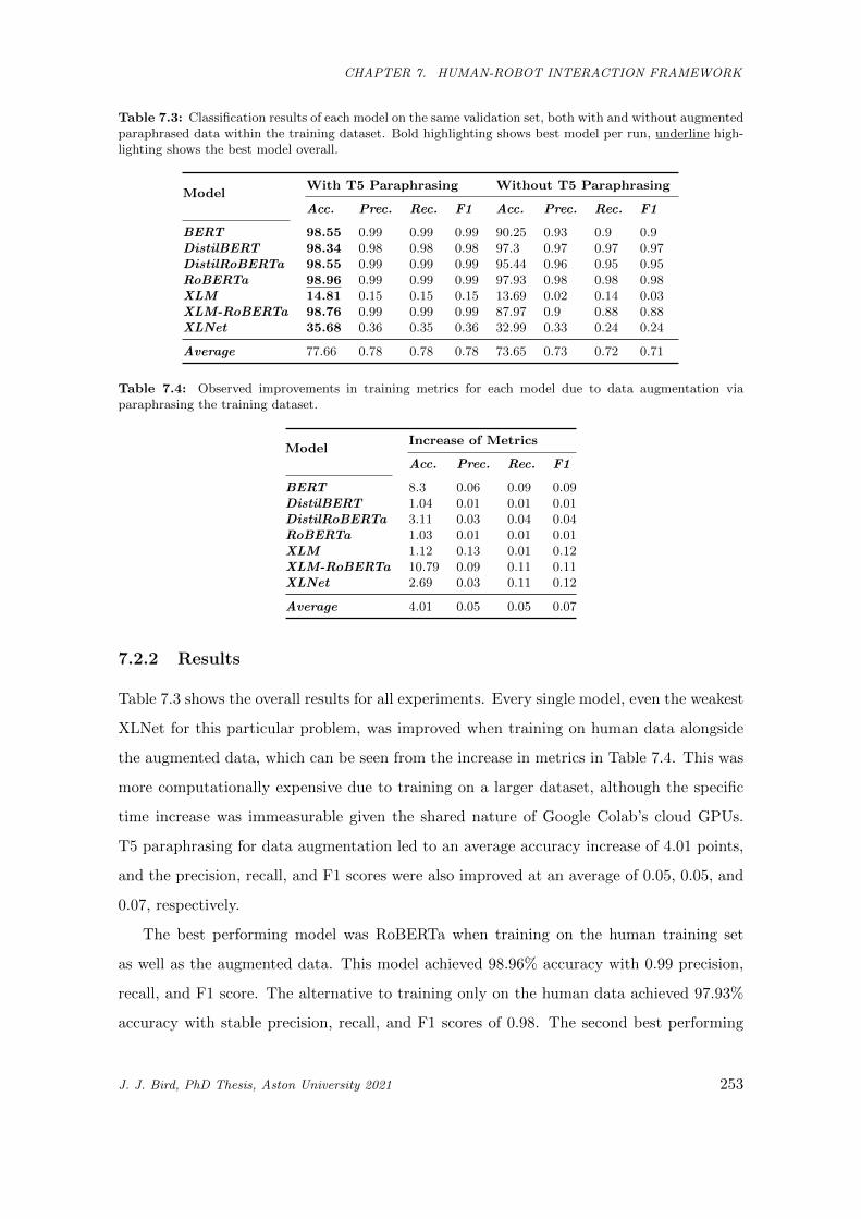
CHAPTER 7. HUMAN-ROBOT INTERACTION FRAMEWORK
Table 7.3: Classification results of each model on the same validation set, both with and without augmentedparaphrased data within the training dataset. Bold highlighting shows best model per run, underline high-lighting shows the best model overall.
ModelWith T5 Paraphrasing Without T5 Paraphrasing
Acc. Prec. Rec. F1 Acc. Prec. Rec. F1
BERT 98.55 0.99 0.99 0.99 90.25 0.93 0.9 0.9DistilBERT 98.34 0.98 0.98 0.98 97.3 0.97 0.97 0.97DistilRoBERTa 98.55 0.99 0.99 0.99 95.44 0.96 0.95 0.95RoBERTa 98.96 0.99 0.99 0.99 97.93 0.98 0.98 0.98XLM 14.81 0.15 0.15 0.15 13.69 0.02 0.14 0.03XLM-RoBERTa 98.76 0.99 0.99 0.99 87.97 0.9 0.88 0.88XLNet 35.68 0.36 0.35 0.36 32.99 0.33 0.24 0.24
Average 77.66 0.78 0.78 0.78 73.65 0.73 0.72 0.71
Table 7.4: Observed improvements in training metrics for each model due to data augmentation viaparaphrasing the training dataset.
ModelIncrease of Metrics
Acc. Prec. Rec. F1
BERT 8.3 0.06 0.09 0.09DistilBERT 1.04 0.01 0.01 0.01DistilRoBERTa 3.11 0.03 0.04 0.04RoBERTa 1.03 0.01 0.01 0.01XLM 1.12 0.13 0.01 0.12XLM-RoBERTa 10.79 0.09 0.11 0.11XLNet 2.69 0.03 0.11 0.12
Average 4.01 0.05 0.05 0.07
7.2.2 Results
Table 7.3 shows the overall results for all experiments. Every single model, even the weakest
XLNet for this particular problem, was improved when training on human data alongside
the augmented data, which can be seen from the increase in metrics in Table 7.4. This was
more computationally expensive due to training on a larger dataset, although the specific
time increase was immeasurable given the shared nature of Google Colab’s cloud GPUs.
T5 paraphrasing for data augmentation led to an average accuracy increase of 4.01 points,
and the precision, recall, and F1 scores were also improved at an average of 0.05, 0.05, and
0.07, respectively.
The best performing model was RoBERTa when training on the human training set
as well as the augmented data. This model achieved 98.96% accuracy with 0.99 precision,
recall, and F1 score. The alternative to training only on the human data achieved 97.93%
accuracy with stable precision, recall, and F1 scores of 0.98. The second best performing
J. J. Bird, PhD Thesis, Aston University 2021 253
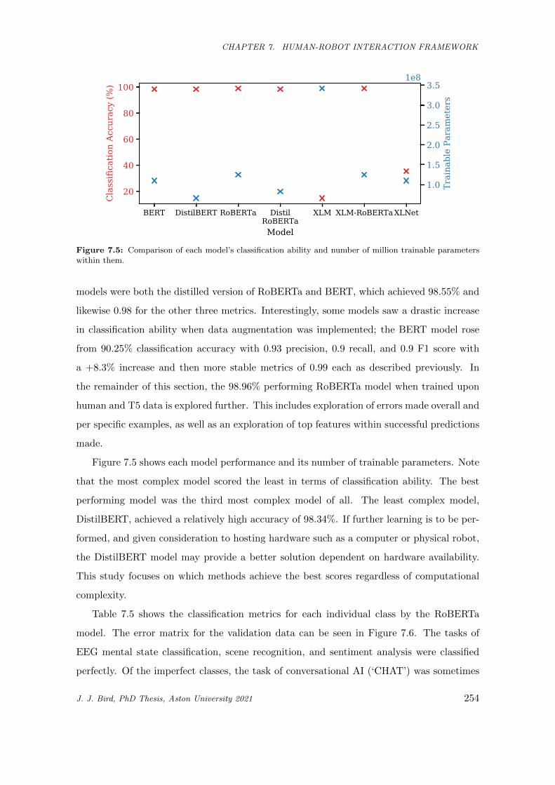
CHAPTER 7. HUMAN-ROBOT INTERACTION FRAMEWORK
BERT DistilBERT RoBERTa DistilRoBERTa
XLM XLM-RoBERTaXLNet
Model
20
40
60
80
100
Cla
ssifi
catio
n Ac
cura
cy (%
)
1.0
1.5
2.0
2.5
3.0
3.5
Trai
nabl
e Pa
ram
eter
s
1e8
Figure 7.5: Comparison of each model’s classification ability and number of million trainable parameterswithin them.
models were both the distilled version of RoBERTa and BERT, which achieved 98.55% and
likewise 0.98 for the other three metrics. Interestingly, some models saw a drastic increase
in classification ability when data augmentation was implemented; the BERT model rose
from 90.25% classification accuracy with 0.93 precision, 0.9 recall, and 0.9 F1 score with
a +8.3% increase and then more stable metrics of 0.99 each as described previously. In
the remainder of this section, the 98.96% performing RoBERTa model when trained upon
human and T5 data is explored further. This includes exploration of errors made overall and
per specific examples, as well as an exploration of top features within successful predictions
made.
Figure 7.5 shows each model performance and its number of trainable parameters. Note
that the most complex model scored the least in terms of classification ability. The best
performing model was the third most complex model of all. The least complex model,
DistilBERT, achieved a relatively high accuracy of 98.34%. If further learning is to be per-
formed, and given consideration to hosting hardware such as a computer or physical robot,
the DistilBERT model may provide a better solution dependent on hardware availability.
This study focuses on which methods achieve the best scores regardless of computational
complexity.
Table 7.5 shows the classification metrics for each individual class by the RoBERTa
model. The error matrix for the validation data can be seen in Figure 7.6. The tasks of
EEG mental state classification, scene recognition, and sentiment analysis were classified
perfectly. Of the imperfect classes, the task of conversational AI (‘CHAT’) was sometimes
J. J. Bird, PhD Thesis, Aston University 2021 254
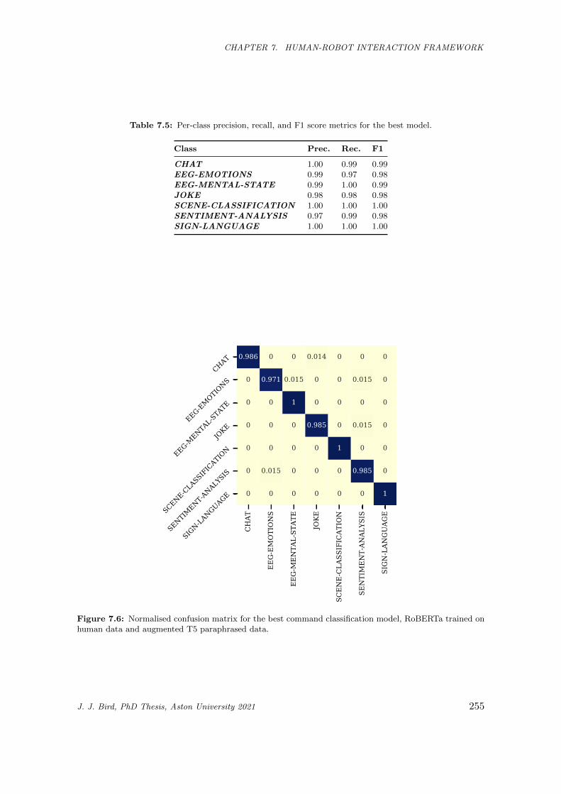
CHAPTER 7. HUMAN-ROBOT INTERACTION FRAMEWORK
Table 7.5: Per-class precision, recall, and F1 score metrics for the best model.
Class Prec. Rec. F1
CHAT 1.00 0.99 0.99EEG-EMOTIONS 0.99 0.97 0.98EEG-MENTAL-STATE 0.99 1.00 0.99JOKE 0.98 0.98 0.98SCENE-CLASSIFICATION 1.00 1.00 1.00SENTIMENT-ANALYSIS 0.97 0.99 0.98SIGN-LANGUAGE 1.00 1.00 1.00
CHAT
EEG-EMOTIONS
EEG-M
ENTA
L-ST
ATE
JOKE
SCENE-CLA
SSIFICAT
ION
SENTIMENT-AN
ALYS
IS
SIGN-LAN
GUAG
E
CHAT
EEG-EM
OTIONS
EEG-ME
NTAL-STATE
JOKE
SCENE-CLASSIFICATION
SENTIMENT-A
NALYSIS
SIGN-LA
NGUAGE
0.986 0 0 0.014 0 0 0
0 0.971 0.015 0 0 0.015 0
0 0 1 0 0 0 0
0 0 0 0.985 0 0.015 0
0 0 0 0 1 0 0
0 0.015 0 0 0 0.985 0
0 0 0 0 0 0 1
Figure 7.6: Normalised confusion matrix for the best command classification model, RoBERTa trained onhuman data and augmented T5 paraphrased data.
J. J. Bird, PhD Thesis, Aston University 2021 255
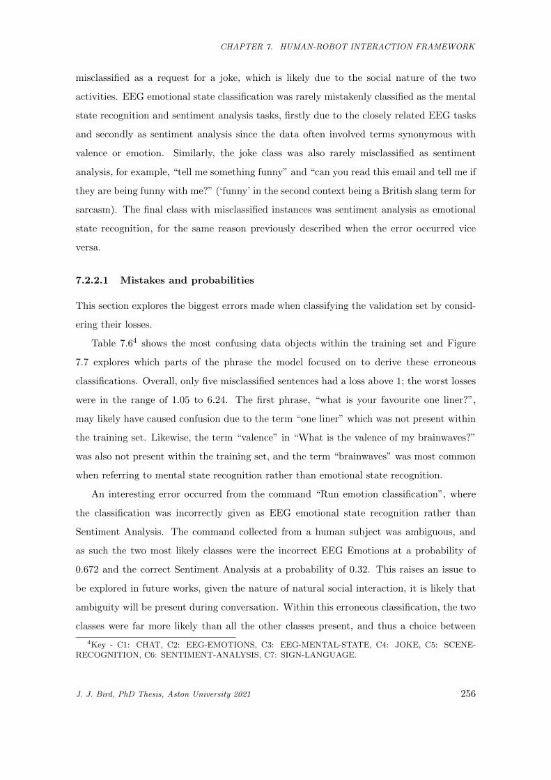
CHAPTER 7. HUMAN-ROBOT INTERACTION FRAMEWORK
misclassified as a request for a joke, which is likely due to the social nature of the two
activities. EEG emotional state classification was rarely mistakenly classified as the mental
state recognition and sentiment analysis tasks, firstly due to the closely related EEG tasks
and secondly as sentiment analysis since the data often involved terms synonymous with
valence or emotion. Similarly, the joke class was also rarely misclassified as sentiment
analysis, for example, “tell me something funny” and “can you read this email and tell me if
they are being funny with me?” (‘funny’ in the second context being a British slang term for
sarcasm). The final class with misclassified instances was sentiment analysis as emotional
state recognition, for the same reason previously described when the error occurred vice
versa.
7.2.2.1 Mistakes and probabilities
This section explores the biggest errors made when classifying the validation set by consid-
ering their losses.
Table 7.64 shows the most confusing data objects within the training set and Figure
7.7 explores which parts of the phrase the model focused on to derive these erroneous
classifications. Overall, only five misclassified sentences had a loss above 1; the worst losses
were in the range of 1.05 to 6.24. The first phrase, “what is your favourite one liner?”,
may likely have caused confusion due to the term “one liner” which was not present within
the training set. Likewise, the term “valence” in “What is the valence of my brainwaves?”
was also not present within the training set, and the term “brainwaves” was most common
when referring to mental state recognition rather than emotional state recognition.
An interesting error occurred from the command “Run emotion classification”, where
the classification was incorrectly given as EEG emotional state recognition rather than
Sentiment Analysis. The command collected from a human subject was ambiguous, and
as such the two most likely classes were the incorrect EEG Emotions at a probability of
0.672 and the correct Sentiment Analysis at a probability of 0.32. This raises an issue to
be explored in future works, given the nature of natural social interaction, it is likely that
ambiguity will be present during conversation. Within this erroneous classification, the two
classes were far more likely than all the other classes present, and thus a choice between
4Key - C1: CHAT, C2: EEG-EMOTIONS, C3: EEG-MENTAL-STATE, C4: JOKE, C5: SCENE-RECOGNITION, C6: SENTIMENT-ANALYSIS, C7: SIGN-LANGUAGE.
J. J. Bird, PhD Thesis, Aston University 2021 256
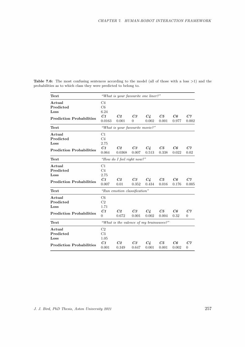
CHAPTER 7. HUMAN-ROBOT INTERACTION FRAMEWORK
Table 7.6: The most confusing sentences according to the model (all of those with a loss >1) and theprobabilities as to which class they were predicted to belong to.
Text “What is your favourite one liner?”
Actual C4Predicted C6Loss 6.24
Prediction ProbabilitiesC1 C2 C3 C4 C5 C6 C70.0163 0.001 0 0.002 0.001 0.977 0.002
Text “What is your favourite movie?”
Actual C1Predicted C4Loss 2.75
Prediction ProbabilitiesC1 C2 C3 C4 C5 C6 C70.064 0.0368 0.007 0.513 0.338 0.022 0.02
Text “How do I feel right now?”
Actual C1Predicted C4Loss 2.75
Prediction ProbabilitiesC1 C2 C3 C4 C5 C6 C70.007 0.01 0.352 0.434 0.016 0.176 0.005
Text “Run emotion classification”
Actual C6Predicted C2Loss 1.71
Prediction ProbabilitiesC1 C2 C3 C4 C5 C6 C70 0.672 0.001 0.002 0.004 0.32 0
Text “What is the valence of my brainwaves?”
Actual C2Predicted C3Loss 1.05
Prediction ProbabilitiesC1 C2 C3 C4 C5 C6 C70.001 0.349 0.647 0.001 0.001 0.002 0
J. J. Bird, PhD Thesis, Aston University 2021 257
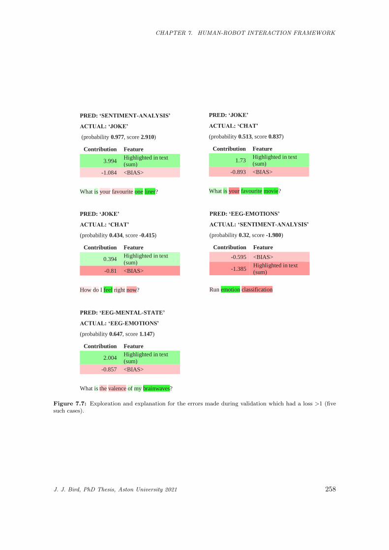
CHAPTER 7. HUMAN-ROBOT INTERACTION FRAMEWORK
PRED: ‘SENTIMENT-ANALYSIS’
ACTUAL: ‘JOKE’
(probability 0.977, score 2.910)
Contribution Feature
3.994 Highlighted in text (sum)
-1.084 <BIAS>
What is your favourite one liner?
PRED: ‘JOKE’
ACTUAL: ‘CHAT’
(probability 0.513, score 0.837)
Contribution Feature
1.73 Highlighted in text (sum)
-0.893 <BIAS>
What is your favourite movie?
PRED: ‘JOKE’
ACTUAL: ‘CHAT’
(probability 0.434, score -0.415)
Contribution Feature
0.394 Highlighted in text (sum)
-0.81 <BIAS>
How do I feel right now?
PRED: ‘EEG-EMOTIONS’
ACTUAL: ‘SENTIMENT-ANALYSIS’
(probability 0.32, score -1.980)
Contribution Feature
-0.595 <BIAS>
-1.385 Highlighted in text (sum)
Run emotion classification
PRED: ‘EEG-MENTAL-STATE’
ACTUAL: ‘EEG-EMOTIONS’
(probability 0.647, score 1.147)
Contribution Feature
2.004 Highlighted in text
(sum)
-0.857 <BIAS>
What is the valence of my brainwaves?
Figure 7.7: Exploration and explanation for the errors made during validation which had a loss >1 (fivesuch cases).
J. J. Bird, PhD Thesis, Aston University 2021 258
CHAPTER 7. HUMAN-ROBOT INTERACTION FRAMEWORK
the two in the form of a question akin to human deduction of ambiguous language would
likely solve such problems and increase accuracy. Additionally, this would rarely incur the
requirement of further effort from the user.
7.2.2.2 Top features within unseen data
Following the training of the model, this section explores the behaviour of the model in the
case of unseen phrases or commands. As such, this serves as more representative of real
scenarios.
Figure 7.8 shows an example correct prediction of each class from previously unseen
data. Interestingly, the model shows behaviour reminiscent of human reading [456, 457]
due to transformers not being limited to considering a temporal sequence in chronological
order of appearance. In the first example, the most useful features were ‘time to speak’
followed by ‘got’, ‘to’ and ’me’. The least useful features were ‘right now’, which alone
would be classified as ‘SCENE-CLASSIFICATION’ with a probability of 0.781 due to many
provided training examples for the class containing questions such as ‘where are you right
now? Can you run scene recognition and tell me?’. The second example also had a strong
negative impact from the word ‘read’ which alone would be classified as ‘SENTIMENT-
ANALYSIS’ with a probability of 0.991 due to phrases such as ‘please read this message
and tell me if they are angry with me’ being popular within the gathered human responses
and as such the augmented data. In this example, the correct classification was found
due to the terms ‘emotions’ and ‘mind’ primarily, followed by ‘feeling’. Following these
two first examples, the remaining five examples were strongly classified. In the mental
state recognition task, even though the term ‘mental state’ was specifically uttered, the
term ‘concentrating’ was the strongest feature within the statement given the goal of the
algorithm to classify concentrating and relaxed states of mind. As could be expected, the
‘JOKE’ task was best classified by the term ‘joke’ itself being present, but, interestingly,
the confidence of classification was increased with the phrases ‘Feeling sad today.’ and
‘cheer me up’. The scene classification task was confidently predicted with a probability
of 1 mainly due to the terms ‘look around’ and ‘where you are’. The red highlight for the
word ‘if’ alone would be classified as ‘SENTIMENT-ANALYSIS’ with a probability of 0.518
given the popularity of phrases along the lines of ‘if they are emotion or emotion’. The
sentiment analysis task was then, again, confidently classified correctly with a probability
J. J. Bird, PhD Thesis, Aston University 2021 259
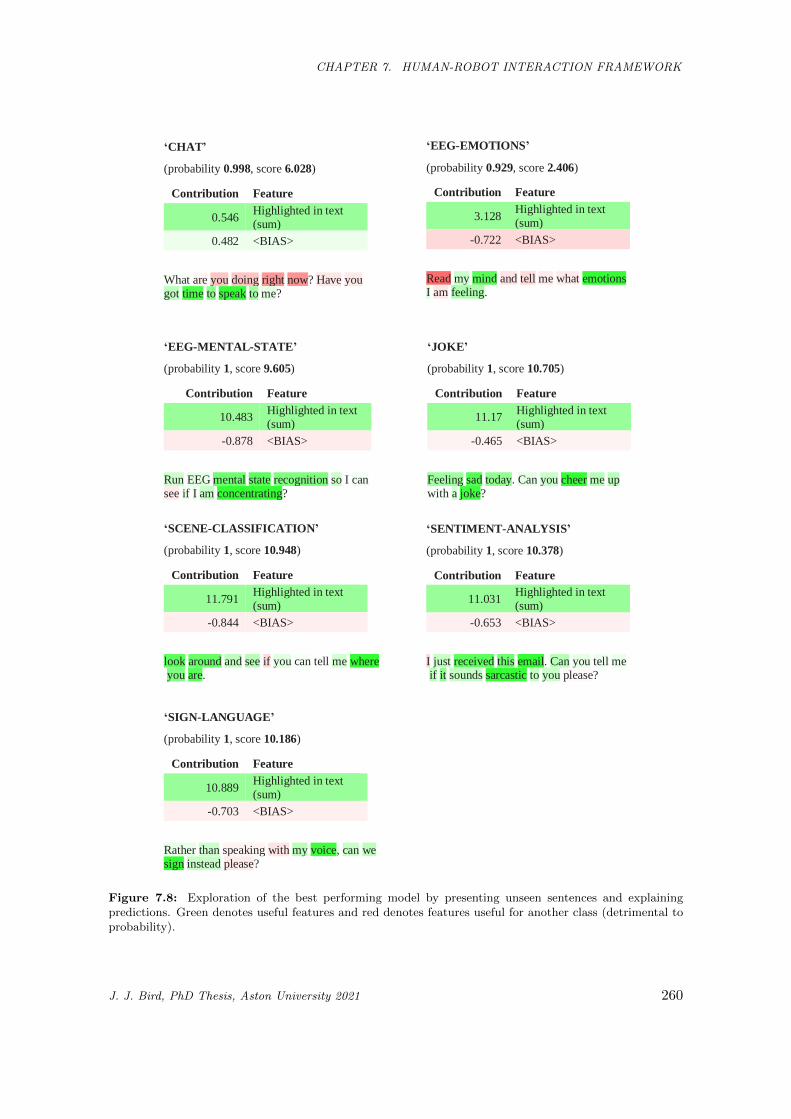
CHAPTER 7. HUMAN-ROBOT INTERACTION FRAMEWORK
‘CHAT’
(probability 0.998, score 6.028)
Contribution Feature
0.546 Highlighted in text (sum)
0.482 <BIAS>
What are you doing right now? Have you got time to speak to me?
‘EEG-EMOTIONS’
(probability 0.929, score 2.406)
Contribution Feature
3.128 Highlighted in text (sum)
-0.722 <BIAS>
Read my mind and tell me what emotions I am feeling.
‘EEG-MENTAL-STATE’
(probability 1, score 9.605)
Contribution Feature
10.483 Highlighted in text (sum)
-0.878 <BIAS>
Run EEG mental state recognition so I can see if I am concentrating?
‘JOKE’
(probability 1, score 10.705)
Contribution Feature
11.17 Highlighted in text (sum)
-0.465 <BIAS>
Feeling sad today. Can you cheer me up with a joke?
‘SCENE-CLASSIFICATION’
(probability 1, score 10.948)
Contribution Feature
11.791 Highlighted in text (sum)
-0.844 <BIAS>
look around and see if you can tell me where you are.
‘SENTIMENT-ANALYSIS’
(probability 1, score 10.378)
Contribution Feature
11.031 Highlighted in text (sum)
-0.653 <BIAS>
I just received this email. Can you tell me if it sounds sarcastic to you please?
‘SIGN-LANGUAGE’
(probability 1, score 10.186)
Contribution Feature
10.889 Highlighted in text (sum)
-0.703 <BIAS>
Rather than speaking with my voice, can we sign instead please?
Figure 7.8: Exploration of the best performing model by presenting unseen sentences and explainingpredictions. Green denotes useful features and red denotes features useful for another class (detrimental toprobability).
J. J. Bird, PhD Thesis, Aston University 2021 260
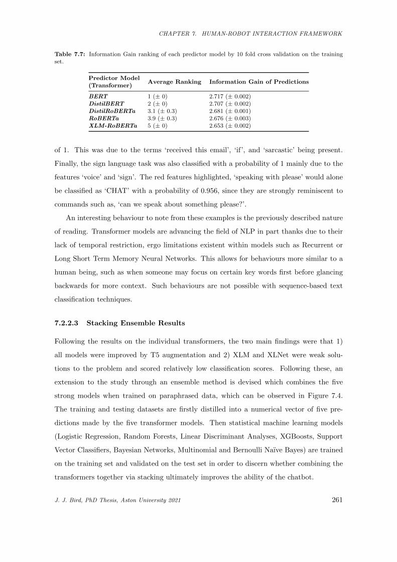
CHAPTER 7. HUMAN-ROBOT INTERACTION FRAMEWORK
Table 7.7: Information Gain ranking of each predictor model by 10 fold cross validation on the trainingset.
Predictor Model(Transformer)
Average Ranking Information Gain of Predictions
BERT 1 (± 0) 2.717 (± 0.002)DistilBERT 2 (± 0) 2.707 (± 0.002)DistilRoBERTa 3.1 (± 0.3) 2.681 (± 0.001)RoBERTa 3.9 (± 0.3) 2.676 (± 0.003)XLM-RoBERTa 5 (± 0) 2.653 (± 0.002)
of 1. This was due to the terms ‘received this email’, ‘if’, and ‘sarcastic’ being present.
Finally, the sign language task was also classified with a probability of 1 mainly due to the
features ‘voice’ and ‘sign’. The red features highlighted, ‘speaking with please’ would alone
be classified as ‘CHAT’ with a probability of 0.956, since they are strongly reminiscent to
commands such as, ‘can we speak about something please?’.
An interesting behaviour to note from these examples is the previously described nature
of reading. Transformer models are advancing the field of NLP in part thanks due to their
lack of temporal restriction, ergo limitations existent within models such as Recurrent or
Long Short Term Memory Neural Networks. This allows for behaviours more similar to a
human being, such as when someone may focus on certain key words first before glancing
backwards for more context. Such behaviours are not possible with sequence-based text
classification techniques.
7.2.2.3 Stacking Ensemble Results
Following the results on the individual transformers, the two main findings were that 1)
all models were improved by T5 augmentation and 2) XLM and XLNet were weak solu-
tions to the problem and scored relatively low classification scores. Following these, an
extension to the study through an ensemble method is devised which combines the five
strong models when trained on paraphrased data, which can be observed in Figure 7.4.
The training and testing datasets are firstly distilled into a numerical vector of five pre-
dictions made by the five transformer models. Then statistical machine learning models
(Logistic Regression, Random Forests, Linear Discriminant Analyses, XGBoosts, Support
Vector Classifiers, Bayesian Networks, Multinomial and Bernoulli Naıve Bayes) are trained
on the training set and validated on the test set in order to discern whether combining the
transformers together via stacking ultimately improves the ability of the chatbot.
J. J. Bird, PhD Thesis, Aston University 2021 261
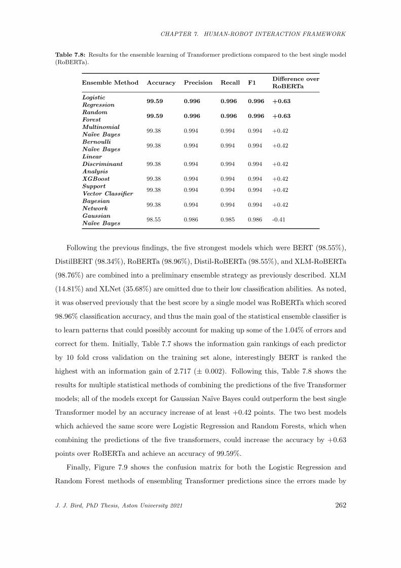
CHAPTER 7. HUMAN-ROBOT INTERACTION FRAMEWORK
Table 7.8: Results for the ensemble learning of Transformer predictions compared to the best single model(RoBERTa).
Ensemble Method Accuracy Precision Recall F1Difference overRoBERTa
LogisticRegression
99.59 0.996 0.996 0.996 +0.63
RandomForest
99.59 0.996 0.996 0.996 +0.63
MultinomialNaıve Bayes
99.38 0.994 0.994 0.994 +0.42
BernoulliNaıve Bayes
99.38 0.994 0.994 0.994 +0.42
LinearDiscriminantAnalysis
99.38 0.994 0.994 0.994 +0.42
XGBoost 99.38 0.994 0.994 0.994 +0.42SupportVector Classifier
99.38 0.994 0.994 0.994 +0.42
BayesianNetwork
99.38 0.994 0.994 0.994 +0.42
GaussianNaıve Bayes
98.55 0.986 0.985 0.986 -0.41
Following the previous findings, the five strongest models which were BERT (98.55%),
DistilBERT (98.34%), RoBERTa (98.96%), Distil-RoBERTa (98.55%), and XLM-RoBERTa
(98.76%) are combined into a preliminary ensemble strategy as previously described. XLM
(14.81%) and XLNet (35.68%) are omitted due to their low classification abilities. As noted,
it was observed previously that the best score by a single model was RoBERTa which scored
98.96% classification accuracy, and thus the main goal of the statistical ensemble classifier is
to learn patterns that could possibly account for making up some of the 1.04% of errors and
correct for them. Initially, Table 7.7 shows the information gain rankings of each predictor
by 10 fold cross validation on the training set alone, interestingly BERT is ranked the
highest with an information gain of 2.717 (± 0.002). Following this, Table 7.8 shows the
results for multiple statistical methods of combining the predictions of the five Transformer
models; all of the models except for Gaussian Naıve Bayes could outperform the best single
Transformer model by an accuracy increase of at least +0.42 points. The two best models
which achieved the same score were Logistic Regression and Random Forests, which when
combining the predictions of the five transformers, could increase the accuracy by +0.63
points over RoBERTa and achieve an accuracy of 99.59%.
Finally, Figure 7.9 shows the confusion matrix for both the Logistic Regression and
Random Forest methods of ensembling Transformer predictions since the errors made by
J. J. Bird, PhD Thesis, Aston University 2021 262
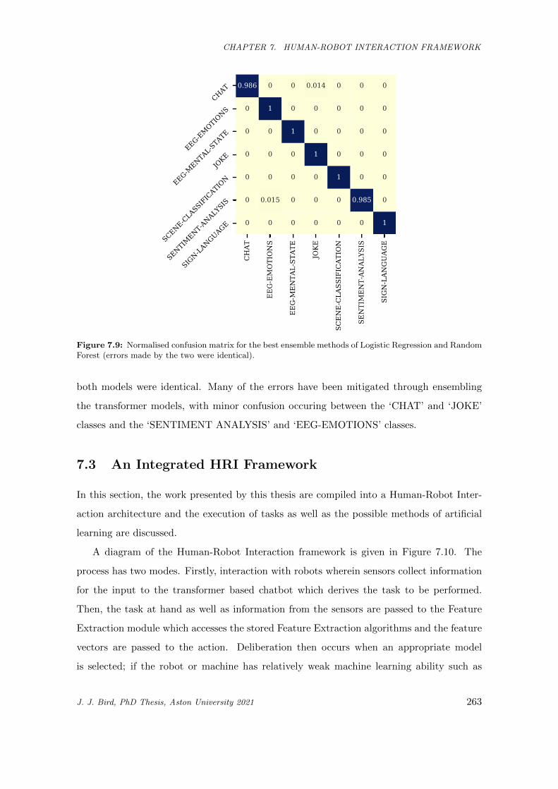
CHAPTER 7. HUMAN-ROBOT INTERACTION FRAMEWORK
CHAT
EEG-EMOTIONS
EEG-M
ENTA
L-ST
ATE
JOKE
SCENE-CLA
SSIFICAT
ION
SENTIMENT-AN
ALYS
IS
SIGN-LAN
GUAG
E
CHAT
EEG-EM
OTIONS
EEG-ME
NTAL-STATE
JOKE
SCENE-CLASSIFICATION
SENTIMENT-A
NALYSIS
SIGN-LA
NGUAGE
0.986 0 0 0.014 0 0 0
0 1 0 0 0 0 0
0 0 1 0 0 0 0
0 0 0 1 0 0 0
0 0 0 0 1 0 0
0 0.015 0 0 0 0.985 0
0 0 0 0 0 0 1
Figure 7.9: Normalised confusion matrix for the best ensemble methods of Logistic Regression and RandomForest (errors made by the two were identical).
both models were identical. Many of the errors have been mitigated through ensembling
the transformer models, with minor confusion occuring between the ‘CHAT’ and ‘JOKE’
classes and the ‘SENTIMENT ANALYSIS’ and ‘EEG-EMOTIONS’ classes.
7.3 An Integrated HRI Framework
In this section, the work presented by this thesis are compiled into a Human-Robot Inter-
action architecture and the execution of tasks as well as the possible methods of artificial
learning are discussed.
A diagram of the Human-Robot Interaction framework is given in Figure 7.10. The
process has two modes. Firstly, interaction with robots wherein sensors collect information
for the input to the transformer based chatbot which derives the task to be performed.
Then, the task at hand as well as information from the sensors are passed to the Feature
Extraction module which accesses the stored Feature Extraction algorithms and the feature
vectors are passed to the action. Deliberation then occurs when an appropriate model
is selected; if the robot or machine has relatively weak machine learning ability such as
J. J. Bird, PhD Thesis, Aston University 2021 263
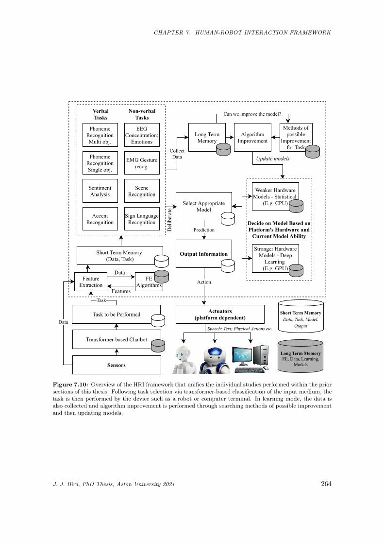
CHAPTER 7. HUMAN-ROBOT INTERACTION FRAMEWORK
DecideonModelBasedonPlatform'sHardwareandCurrentModelAbility
Task
TasktobePerformedData
Sensors
Actuators(platformdependent)
FeatureExtraction
FEAlgorithms
Data
Features
Transformer-basedChatbot
VerbalTasks
Non-verbalTasks
EEGConcentration;Emotions
EMGGesturerecog.
Speech;Text;PhysicalActionsetc.
PhonemeRecognitionSingleobj.
PhonemeRecognitionMultiobj.
AccentRecognition
SentimentAnalysis
SceneRecognition
SignLanguageRecognition
AlgorithmImprovement
Prediction
SelectAppropriateModel
WeakerHardwareModels-Statistical
(E.g.CPU)
StrongerHardwareModels-DeepLearning(E.g.GPU)
Canweimprovethemodel?
LongTermMemory
Updatemodels
Action
OutputInformation
CollectData
ShortTermMemory(Data,Task)
Methodsofpossible
ImprovementforTask
ShortTermMemoryData,Task,Model,
Output
LongTermMemoryFE,Data,Learning,
Models
Deliberate
Figure 7.10: Overview of the HRI framework that unifies the individual studies performed within the priorsections of this thesis. Following task selection via transformer-based classification of the input medium, thetask is then performed by the device such as a robot or computer terminal. In learning mode, the data isalso collected and algorithm improvement is performed through searching methods of possible improvementand then updating models.
J. J. Bird, PhD Thesis, Aston University 2021 264
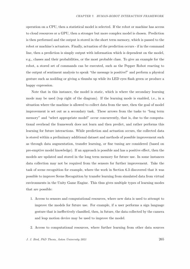
CHAPTER 7. HUMAN-ROBOT INTERACTION FRAMEWORK
operation on a CPU, then a statistical model is selected. If the robot or machine has access
to cloud resources or a GPU, then a stronger but more complex model is chosen. Prediction
is then performed and the output is stored in the short term memory, which is passed to the
robot or machine’s actuators. Finally, actuation of the prediction occurs - if in the command
line, then a prediction is simply output with information which is dependent on the model,
e.g., classes and their probabilities, or the most probable class. To give an example for the
robot, a stored set of commands can be executed, such as the Pepper Robot reacting to
the output of sentiment analysis to speak “the message is positive!” and perform a physical
gesture such as nodding or giving a thumbs up while its LED eyes flash green or produce a
happy expression.
Note that in this instance, the model is static, which is where the secondary learning
mode may be used (top right of the diagram). If the learning mode is enabled, i.e., in a
situation where the machine is allowed to collect data from the user, then the goal of model
improvement is set out as a secondary task. These arrows from the tasks to “long term
memory” and “select appropriate model” occur concurrently, that is, due to the computa-
tional overhead the framework does not learn and then predict, and rather performs this
learning for future interactions. While prediction and actuation occurs, the collected data
is stored within a preliminary additional dataset and methods of possible improvement such
as through data augmentation, transfer learning, or fine tuning are considered (based on
pre-emptive model knowledge). If an approach is possible and has a positive effect, then the
models are updated and stored in the long term memory for future use. In some instances
data collection may not be required from the sensors for further improvement. Take the
task of scene recognition for example, where the work in Section 6.3 discovered that it was
possible to improve Scene Recognition by transfer learning from simulated data from virtual
environments in the Unity Game Engine. This thus gives multiple types of learning modes
that are possible:
1. Access to sensors and computational resources, where new data is used to attempt to
improve the models for future use. For example, if a user performs a sign language
gesture that is ineffectively classified, then, in future, the data collected by the camera
and leap motion device may be used to improve the model.
2. Access to computational resources, where further learning from other data sources
J. J. Bird, PhD Thesis, Aston University 2021 265
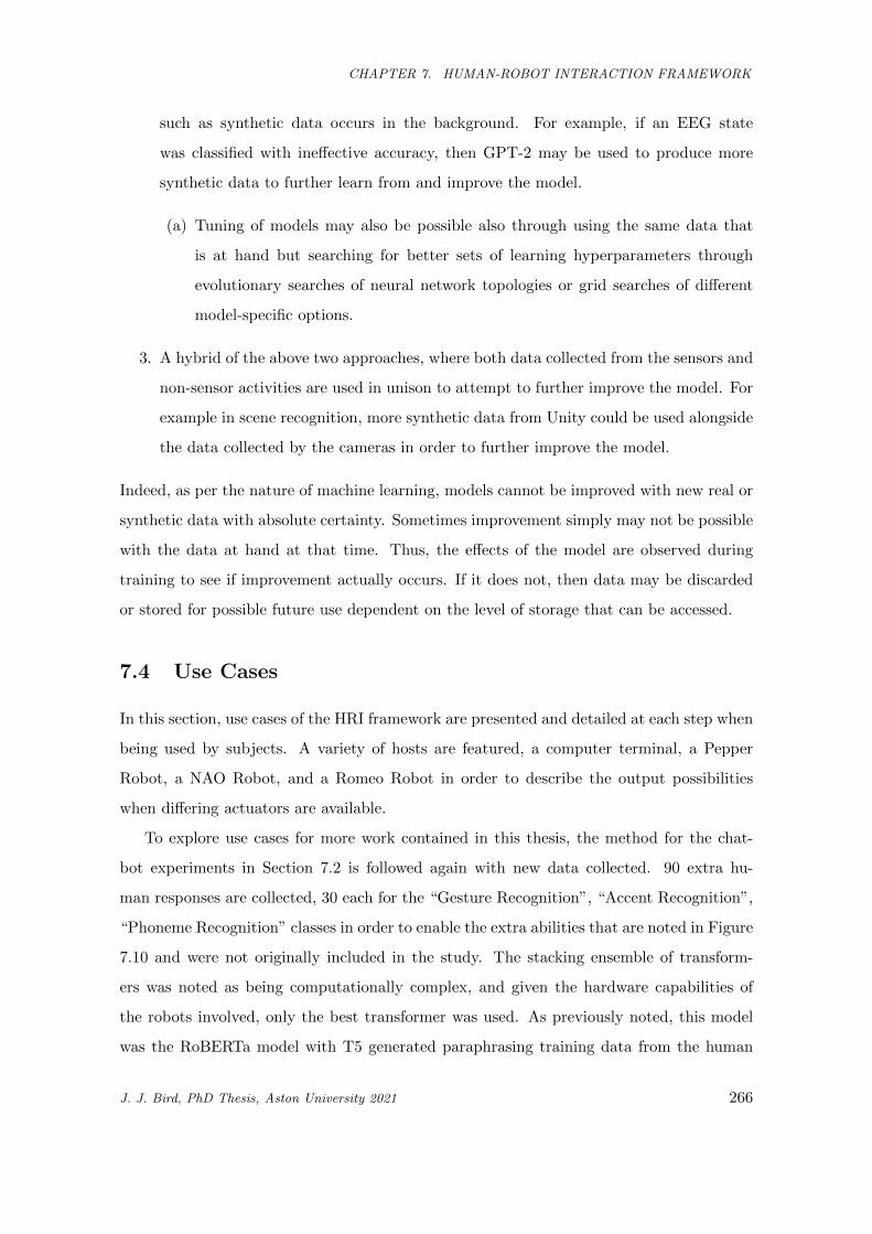
CHAPTER 7. HUMAN-ROBOT INTERACTION FRAMEWORK
such as synthetic data occurs in the background. For example, if an EEG state
was classified with ineffective accuracy, then GPT-2 may be used to produce more
synthetic data to further learn from and improve the model.
(a) Tuning of models may also be possible also through using the same data that
is at hand but searching for better sets of learning hyperparameters through
evolutionary searches of neural network topologies or grid searches of different
model-specific options.
3. A hybrid of the above two approaches, where both data collected from the sensors and
non-sensor activities are used in unison to attempt to further improve the model. For
example in scene recognition, more synthetic data from Unity could be used alongside
the data collected by the cameras in order to further improve the model.
Indeed, as per the nature of machine learning, models cannot be improved with new real or
synthetic data with absolute certainty. Sometimes improvement simply may not be possible
with the data at hand at that time. Thus, the effects of the model are observed during
training to see if improvement actually occurs. If it does not, then data may be discarded
or stored for possible future use dependent on the level of storage that can be accessed.
7.4 Use Cases
In this section, use cases of the HRI framework are presented and detailed at each step when
being used by subjects. A variety of hosts are featured, a computer terminal, a Pepper
Robot, a NAO Robot, and a Romeo Robot in order to describe the output possibilities
when differing actuators are available.
To explore use cases for more work contained in this thesis, the method for the chat-
bot experiments in Section 7.2 is followed again with new data collected. 90 extra hu-
man responses are collected, 30 each for the “Gesture Recognition”, “Accent Recognition”,
“Phoneme Recognition” classes in order to enable the extra abilities that are noted in Figure
7.10 and were not originally included in the study. The stacking ensemble of transform-
ers was noted as being computationally complex, and given the hardware capabilities of
the robots involved, only the best transformer was used. As previously noted, this model
was the RoBERTa model with T5 generated paraphrasing training data from the human
J. J. Bird, PhD Thesis, Aston University 2021 266
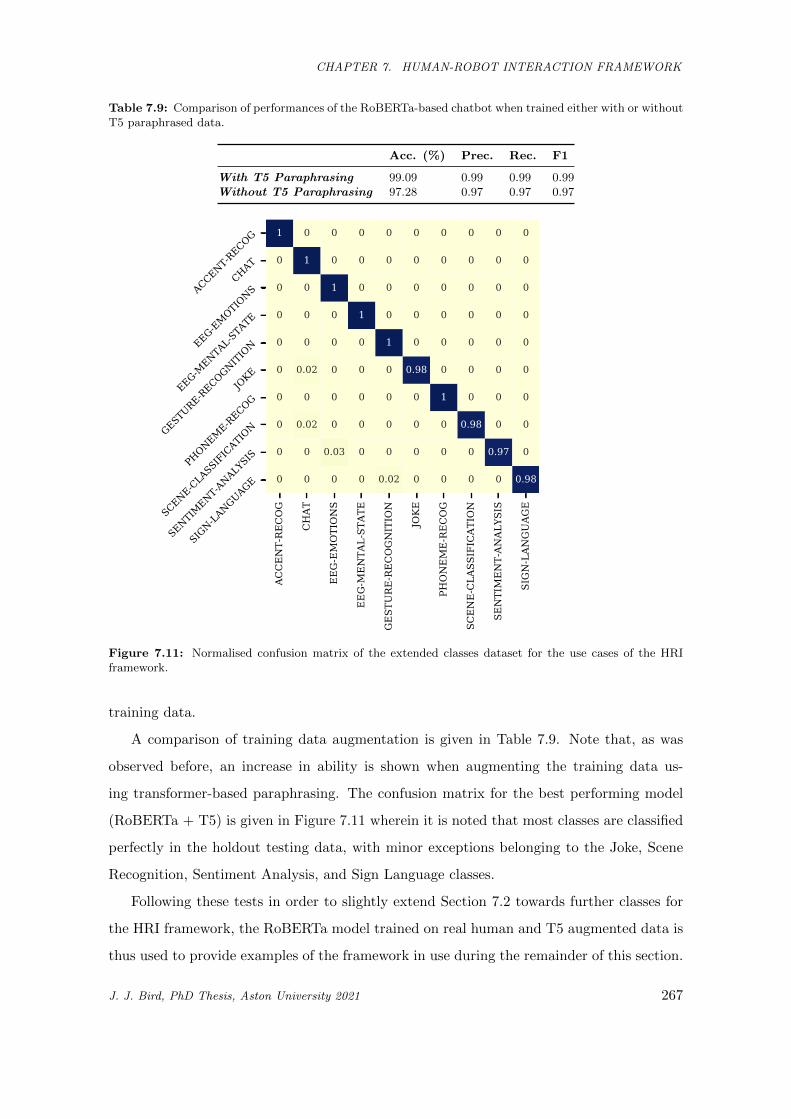
CHAPTER 7. HUMAN-ROBOT INTERACTION FRAMEWORK
Table 7.9: Comparison of performances of the RoBERTa-based chatbot when trained either with or withoutT5 paraphrased data.
Acc. (%) Prec. Rec. F1
With T5 Paraphrasing 99.09 0.99 0.99 0.99Without T5 Paraphrasing 97.28 0.97 0.97 0.97
ACCENT-RECOG
CHAT
EEG-EMOTIONS
EEG-M
ENTA
L-ST
ATE
GEST
URE-RECOGNITIO
N
JOKE
PHONEME-RECOG
SCENE-CLA
SSIFICAT
ION
SENTIMENT-AN
ALYS
IS
SIGN-LAN
GUAG
E
ACCENT-RECOG
CHAT
EEG-EM
OTIONS
EEG-ME
NTAL-STATE
GESTURE-RECOGNITION
JOKE
PHONEM
E-RECOG
SCENE-CLASSIFICATION
SENTIMENT-A
NALYSIS
SIGN-LA
NGUAGE
1 0 0 0 0 0 0 0 0 0
0 1 0 0 0 0 0 0 0 0
0 0 1 0 0 0 0 0 0 0
0 0 0 1 0 0 0 0 0 0
0 0 0 0 1 0 0 0 0 0
0 0.02 0 0 0 0.98 0 0 0 0
0 0 0 0 0 0 1 0 0 0
0 0.02 0 0 0 0 0 0.98 0 0
0 0 0.03 0 0 0 0 0 0.97 0
0 0 0 0 0.02 0 0 0 0 0.98
Figure 7.11: Normalised confusion matrix of the extended classes dataset for the use cases of the HRIframework.
training data.
A comparison of training data augmentation is given in Table 7.9. Note that, as was
observed before, an increase in ability is shown when augmenting the training data us-
ing transformer-based paraphrasing. The confusion matrix for the best performing model
(RoBERTa + T5) is given in Figure 7.11 wherein it is noted that most classes are classified
perfectly in the holdout testing data, with minor exceptions belonging to the Joke, Scene
Recognition, Sentiment Analysis, and Sign Language classes.
Following these tests in order to slightly extend Section 7.2 towards further classes for
the HRI framework, the RoBERTa model trained on real human and T5 augmented data is
thus used to provide examples of the framework in use during the remainder of this section.
J. J. Bird, PhD Thesis, Aston University 2021 267
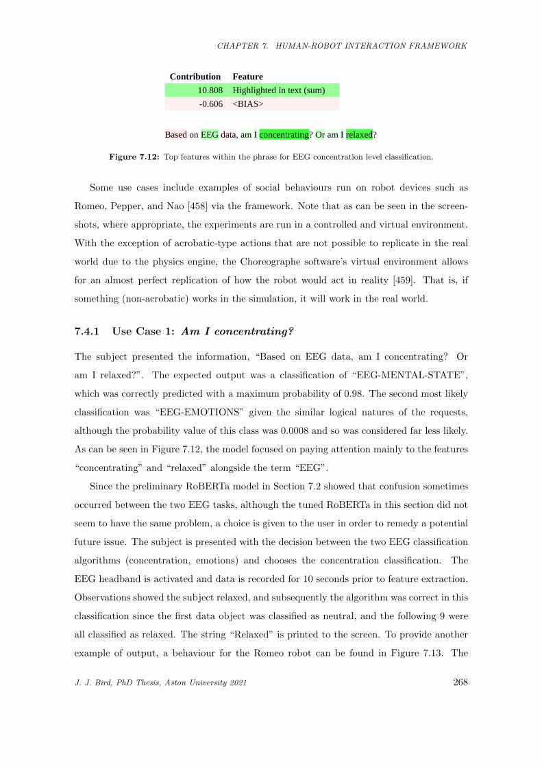
CHAPTER 7. HUMAN-ROBOT INTERACTION FRAMEWORK
EEG-MENTAL-STATE
Contribution Feature
10.808 Highlighted in text (sum)
-0.606 <BIAS>
Based on EEG data, am I concentrating? Or am I relaxed?
Contribution Feature
8.919 Highlighted in text (sum)
-0.523 <BIAS>
Is this text good or bad in terms of sentiment?
Contribution Feature
11.414 Highlighted in text (sum)
-0.821 <BIAS>
Rather than speaking, can we use sign language instead?
Contribution Feature
8.995 Highlighted in text (sum)
-0.095 <BIAS>
Take a look around and run multimodal scene recognition.
Figure 7.12: Top features within the phrase for EEG concentration level classification.
Some use cases include examples of social behaviours run on robot devices such as
Romeo, Pepper, and Nao [458] via the framework. Note that as can be seen in the screen-
shots, where appropriate, the experiments are run in a controlled and virtual environment.
With the exception of acrobatic-type actions that are not possible to replicate in the real
world due to the physics engine, the Choreographe software’s virtual environment allows
for an almost perfect replication of how the robot would act in reality [459]. That is, if
something (non-acrobatic) works in the simulation, it will work in the real world.
7.4.1 Use Case 1: Am I concentrating?
The subject presented the information, “Based on EEG data, am I concentrating? Or
am I relaxed?”. The expected output was a classification of “EEG-MENTAL-STATE”,
which was correctly predicted with a maximum probability of 0.98. The second most likely
classification was “EEG-EMOTIONS” given the similar logical natures of the requests,
although the probability value of this class was 0.0008 and so was considered far less likely.
As can be seen in Figure 7.12, the model focused on paying attention mainly to the features
“concentrating” and “relaxed” alongside the term “EEG”.
Since the preliminary RoBERTa model in Section 7.2 showed that confusion sometimes
occurred between the two EEG tasks, although the tuned RoBERTa in this section did not
seem to have the same problem, a choice is given to the user in order to remedy a potential
future issue. The subject is presented with the decision between the two EEG classification
algorithms (concentration, emotions) and chooses the concentration classification. The
EEG headband is activated and data is recorded for 10 seconds prior to feature extraction.
Observations showed the subject relaxed, and subsequently the algorithm was correct in this
classification since the first data object was classified as neutral, and the following 9 were
all classified as relaxed. The string “Relaxed” is printed to the screen. To provide another
example of output, a behaviour for the Romeo robot can be found in Figure 7.13. The
J. J. Bird, PhD Thesis, Aston University 2021 268
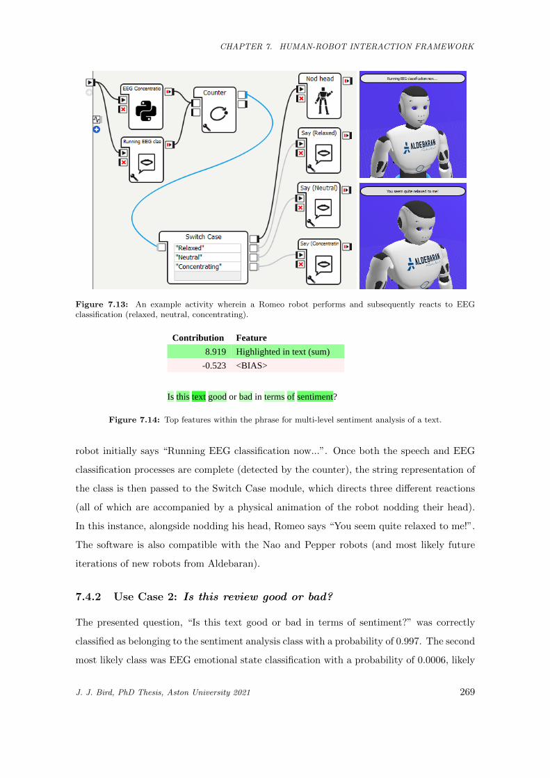
CHAPTER 7. HUMAN-ROBOT INTERACTION FRAMEWORK
Figure 7.13: An example activity wherein a Romeo robot performs and subsequently reacts to EEGclassification (relaxed, neutral, concentrating).
EEG-MENTAL-STATE
Contribution Feature
10.808 Highlighted in text (sum)
-0.606 <BIAS>
Based on EEG data, am I concentrating? Or am I relaxed?
Contribution Feature
8.919 Highlighted in text (sum)
-0.523 <BIAS>
Is this text good or bad in terms of sentiment?
Contribution Feature
11.414 Highlighted in text (sum)
-0.821 <BIAS>
Rather than speaking, can we use sign language instead?
Contribution Feature
8.995 Highlighted in text (sum)
-0.095 <BIAS>
Take a look around and run multimodal scene recognition.
Figure 7.14: Top features within the phrase for multi-level sentiment analysis of a text.
robot initially says “Running EEG classification now...”. Once both the speech and EEG
classification processes are complete (detected by the counter), the string representation of
the class is then passed to the Switch Case module, which directs three different reactions
(all of which are accompanied by a physical animation of the robot nodding their head).
In this instance, alongside nodding his head, Romeo says “You seem quite relaxed to me!”.
The software is also compatible with the Nao and Pepper robots (and most likely future
iterations of new robots from Aldebaran).
7.4.2 Use Case 2: Is this review good or bad?
The presented question, “Is this text good or bad in terms of sentiment?” was correctly
classified as belonging to the sentiment analysis class with a probability of 0.997. The second
most likely class was EEG emotional state classification with a probability of 0.0006, likely
J. J. Bird, PhD Thesis, Aston University 2021 269
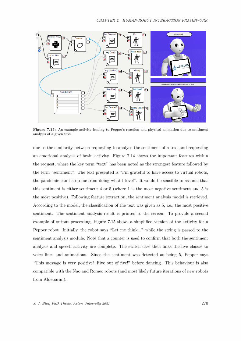
CHAPTER 7. HUMAN-ROBOT INTERACTION FRAMEWORK
Figure 7.15: An example activity leading to Pepper’s reaction and physical animation due to sentimentanalysis of a given text.
due to the similarity between requesting to analyse the sentiment of a text and requesting
an emotional analysis of brain activity. Figure 7.14 shows the important features within
the request, where the key term “text” has been noted as the strongest feature followed by
the term “sentiment”. The text presented is “I’m grateful to have access to virtual robots,
the pandemic can’t stop me from doing what I love!”. It would be sensible to assume that
this sentiment is either sentiment 4 or 5 (where 1 is the most negative sentiment and 5 is
the most positive). Following feature extraction, the sentiment analysis model is retrieved.
According to the model, the classification of the text was given as 5, i.e., the most positive
sentiment. The sentiment analysis result is printed to the screen. To provide a second
example of output processing, Figure 7.15 shows a simplified version of the activity for a
Pepper robot. Initially, the robot says “Let me think...” while the string is passed to the
sentiment analysis module. Note that a counter is used to confirm that both the sentiment
analysis and speech activity are complete. The switch case then links the five classes to
voice lines and animations. Since the sentiment was detected as being 5, Pepper says
“This message is very positive! Five out of five!” before dancing. This behaviour is also
compatible with the Nao and Romeo robots (and most likely future iterations of new robots
from Aldebaran).
J. J. Bird, PhD Thesis, Aston University 2021 270
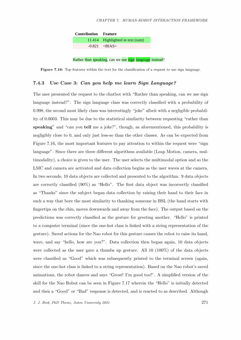
CHAPTER 7. HUMAN-ROBOT INTERACTION FRAMEWORK
EEG-MENTAL-STATE
Contribution Feature
10.808 Highlighted in text (sum)
-0.606 <BIAS>
Based on EEG data, am I concentrating? Or am I relaxed?
Contribution Feature
8.919 Highlighted in text (sum)
-0.523 <BIAS>
Is this text good or bad in terms of sentiment?
Contribution Feature
11.414 Highlighted in text (sum)
-0.821 <BIAS>
Rather than speaking, can we use sign language instead?
Contribution Feature
8.995 Highlighted in text (sum)
-0.095 <BIAS>
Take a look around and run multimodal scene recognition.
Figure 7.16: Top features within the text for the classification of a request to use sign language.
7.4.3 Use Case 3: Can you help me learn Sign Language?
The user presented the request to the chatbot with “Rather than speaking, can we use sign
language instead?”. The sign language class was correctly classified with a probability of
0.998, the second most likely class was interestingly “joke” albeit with a negligible probabil-
ity of 0.0003. This may be due to the statistical similarity between requesting “rather than
speaking” and “can you tell me a joke?”, though, as aforementioned, this probability is
negligibly close to 0, and only just less-so than the other classes. As can be expected from
Figure 7.16, the most important features to pay attention to within the request were “sign
language”. Since there are three different algorithms available (Leap Motion, camera, mul-
timodality), a choice is given to the user. The user selects the multimodal option and so the
LMC and camera are activated and data collection begins as the user waves at the camera.
In two seconds, 10 data objects are collected and presented to the algorithm. 9 data objects
are correctly classified (90%) as “Hello”. The first data object was incorrectly classified
as “Thanks” since the subject began data collection by raising their hand to their face in
such a way that bore the most similarity to thanking someone in BSL (the hand starts with
fingertips on the chin, moves downwards and away from the face). The output based on the
predictions was correctly classified as the gesture for greeting another. “Hello” is printed
to a computer terminal (since the one-hot class is linked with a string representation of the
gesture). Saved actions for the Nao robot for this gesture causes the robot to raise its hand,
wave, and say “hello, how are you?”. Data collection then began again, 10 data objects
were collected as the user gave a thumbs up gesture. All 10 (100%) of the data objects
were classified as “Good” which was subsequently printed to the terminal screen (again,
since the one-hot class is linked to a string representation). Based on the Nao robot’s saved
animations, the robot dances and says “Great! I’m good too!”. A simplified version of the
skill for the Nao Robot can be seen in Figure 7.17 wherein the “Hello” is initially detected
and then a “Good” or “Bad” response is detected, and is reacted to as described. Although
J. J. Bird, PhD Thesis, Aston University 2021 271
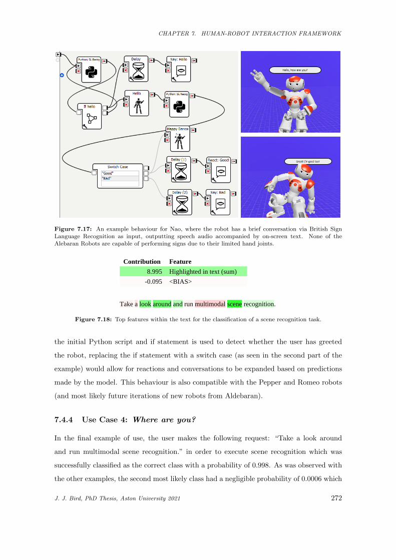
CHAPTER 7. HUMAN-ROBOT INTERACTION FRAMEWORK
Figure 7.17: An example behaviour for Nao, where the robot has a brief conversation via British SignLanguage Recognition as input, outputting speech audio accompanied by on-screen text. None of theAlebaran Robots are capable of performing signs due to their limited hand joints.
EEG-MENTAL-STATE
Contribution Feature
10.808 Highlighted in text (sum)
-0.606 <BIAS>
Based on EEG data, am I concentrating? Or am I relaxed?
Contribution Feature
8.919 Highlighted in text (sum)
-0.523 <BIAS>
Is this text good or bad in terms of sentiment?
Contribution Feature
11.414 Highlighted in text (sum)
-0.821 <BIAS>
Rather than speaking, can we use sign language instead?
Contribution Feature
8.995 Highlighted in text (sum)
-0.095 <BIAS>
Take a look around and run multimodal scene recognition.
Figure 7.18: Top features within the text for the classification of a scene recognition task.
the initial Python script and if statement is used to detect whether the user has greeted
the robot, replacing the if statement with a switch case (as seen in the second part of the
example) would allow for reactions and conversations to be expanded based on predictions
made by the model. This behaviour is also compatible with the Pepper and Romeo robots
(and most likely future iterations of new robots from Aldebaran).
7.4.4 Use Case 4: Where are you?
In the final example of use, the user makes the following request: “Take a look around
and run multimodal scene recognition.” in order to execute scene recognition which was
successfully classified as the correct class with a probability of 0.998. As was observed with
the other examples, the second most likely class had a negligible probability of 0.0006 which
J. J. Bird, PhD Thesis, Aston University 2021 272
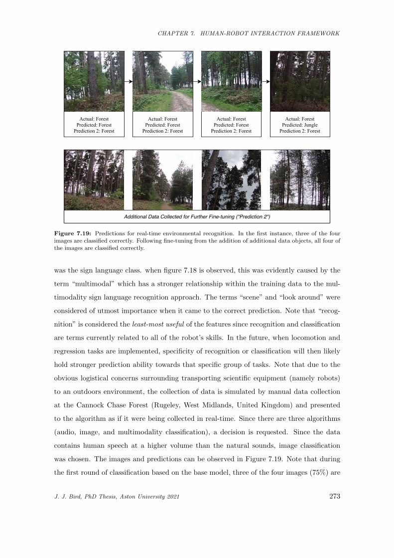
CHAPTER 7. HUMAN-ROBOT INTERACTION FRAMEWORK
Actual:ForestPredicted:ForestPrediction2:Forest
Actual:ForestPredicted:ForestPrediction2:Forest
Actual:ForestPredicted:ForestPrediction2:Forest
Actual:ForestPredicted:JunglePrediction2:Forest
Additional Data Collected for Further Fine-tuning ("Prediction 2")
Figure 7.19: Predictions for real-time environmental recognition. In the first instance, three of the fourimages are classified correctly. Following fine-tuning from the addition of additional data objects, all four ofthe images are classified correctly.
was the sign language class. when figure 7.18 is observed, this was evidently caused by the
term “multimodal” which has a stronger relationship within the training data to the mul-
timodality sign language recognition approach. The terms “scene” and “look around” were
considered of utmost importance when it came to the correct prediction. Note that “recog-
nition” is considered the least-most useful of the features since recognition and classification
are terms currently related to all of the robot’s skills. In the future, when locomotion and
regression tasks are implemented, specificity of recognition or classification will then likely
hold stronger prediction ability towards that specific group of tasks. Note that due to the
obvious logistical concerns surrounding transporting scientific equipment (namely robots)
to an outdoors environment, the collection of data is simulated by manual data collection
at the Cannock Chase Forest (Rugeley, West Midlands, United Kingdom) and presented
to the algorithm as if it were being collected in real-time. Since there are three algorithms
(audio, image, and multimodality classification), a decision is requested. Since the data
contains human speech at a higher volume than the natural sounds, image classification
was chosen. The images and predictions can be observed in Figure 7.19. Note that during
the first round of classification based on the base model, three of the four images (75%) are
J. J. Bird, PhD Thesis, Aston University 2021 273
CHAPTER 7. HUMAN-ROBOT INTERACTION FRAMEWORK
correctly classified as ‘forest’. One of the images was incorrectly classified as the ‘jungle’ en-
vironment, possibly due to the auto-focus of the camera lowering the exposure and making
the image darker (giving the impression that the natural environment is more overgrown
than it actually is). The output of the process, thus, is the correct classification, the model
has recognised the forest environment. Since an error was made, further data was collected
and added to the dataset for slight further fine-tuning of the image recognition model for
1 epoch and the data was presented to this new model, where the model achieved 100% by
correctly classifying all images.
7.5 Summary and Conclusion
To summarise, the studies in Section 7.2 show primarily that data augmentation through
transformer-based paraphrasing via the T5 model improve many state-of-the-art language
transformer-based classification models. BERT and DistilBERT, RoBERTa and Disil-
RoBERTa, XLM, XLM-RoBERTa, and XLNet all showed increases in learning performance
when learning with augmented data from the training set when compared to learning only
on the original data pre-augmentation. The best single model found was RoBERTa, which
could classify human commands to an artificially intelligent system at a rate of 98.96%
accuracy, where errors were often due to ambiguity within human language. A statistical
ensemble of the five best transformer models then led to an increased accuracy of 99.59%
when using either Logistic Regression or a Random Forest to process the output predic-
tions of each transformer, utilising small differences between the models when trained on
the dataset. Although XLM did not perform well, the promising performance of XLM-
RoBERTa showed that models trained on a task do not necessarily underperform on an-
other different task given the general ability of lingual understanding. With this in mind,
and given that the models are too complex to train simultaneously, it may be useful in
the future to consider the predictions of all trained models and form an ensemble through
meta-classifiers through statistical, deep learning, or further transformer approaches. A
small vector input of predictions would allow for deeper decision making given the singular
outputs of each transformer. Alternatively, a vector of inputs in addition to the original
text may allow for deeper understanding behind why errors are made and allow for learned
exceptions to overcome them. A preliminary ensemble of the five models that did not have
J. J. Bird, PhD Thesis, Aston University 2021 274
CHAPTER 7. HUMAN-ROBOT INTERACTION FRAMEWORK
weak scores showed that classification accuracy could be further increased by treating the
outputs of each transformer model as attributes in themselves for rules to be learnt from.
The experiments in this part of the thesis were limited in that attribute selection was based
solely on removing the two underperforming models; in the future, exploration could be
performed on attribute selection to fine-tune the number of models used as input. Addi-
tionally, only a predicted label in the form of nominal attributes were used as input, whereas
additional attributes such as probabilities of each output class could be utilised to provide
more information for the statistical ensemble classifier.
To conclude this part of the thesis, this chapter has initially presented a transformer-
based chatbot framework to provide socially-interactive accessibility to the individual abil-
ities that the robot possesses. All of the work performed in this thesis was then integrated
into the overall framework, and several examples were given on its operation.
The primary and final aim of this thesis, an integration into a framework allowing
emergence of behaviours more than a sum of their parts, has been presented in this chapter.
Individual machine learning tasks are now enabled through natural conversation with a
machine, and four different platforms including three physical robots (Personal Computer,
Romeo, Pepper, Nao) have shown success when running the framework in real-time by
being requested to, and interpreting their surroundings through a variation of sensors and
algorithms.
J. J. Bird, PhD Thesis, Aston University 2021 275
CHAPTER 8. DISCUSSION AND CONCLUSION
Chapter 8
Discussion and Conclusion
8.1 Revisiting Open Issues
As was discussed previously during literature review, prominent works in the field have
generally suggested for guidelines to be followed in order to remedy open issues in the field of
HRI. Here, those guidelines are repeated prior to a discussion concerning this work. Fischer
et al.[28] and Drury et al.[32] presented guidelines that HRI frameworks should aim to follow.
These suggestions were based on the observation of open issues that currently impede the
field of HRI, and as such the framework in this thesis set out to remedy them. This section
reiterates said guidelines and discusses the ways in which the framework presented by this
thesis either implements them directly or allows for support of their implementation. The
discussion in this chapter centres around research question 3, “Which current open issues
in Human-Robot Interaction can be alleviated by the framework presented in this thesis?
And to what extent?”.
8.1.1 Adaptability and ease of use
Adaption to related problems and robotic devices should be easy to implement. Cross-
dependency should be minimal in order to enable substitution.
As was previously shown, robotic devices are easy to implement, since the framework can
act as an API-like software which outputs learning information (i.e. prediction, accuracy and
classification metrics) and this can be used independently between devices. As was shown
in the case studies, a terminal can output the predictions based on a user’s request, whereas
J. J. Bird, PhD Thesis, Aston University 2021 276
CHAPTER 8. DISCUSSION AND CONCLUSION
the robots can provide more output through speech and physical movement via the libraries
provided by Softbank. In most cases (except for image recognition), several different models
are available to use based on the computational capabilities of the hosting computer or robot.
Thus, dependencies on hardware are mitigated since a model is autonomously chosen from
a memory containing several deep learning and classical machine learning approaches. This
is also the case with model improvement, for example, a Nao Robot’s Intel Atom Z530
(1 core, 1.6GHz) CPU is unable to run a GPT-2 training and generation instance and
thus this data augmentation should not be chosen as the method for model improvement.
Ease of use is further implemented through the transformer-based chatbot, which allows for
natural interaction in place of programming. As was observed during case studies, the users
naturally requested a routine through a spoken manner of their choice, and the model was
confident as to what their requests actually were, thus classifying it accurately. As such,
the design of the framework and integrated technologies allow for both adaptability and
ease of use.
8.1.2 Provision of overall framework
The provided framework should work as-is and as such provide useful routines and goals.
The framework that was presented following supporting research project indeed pos-
sesses several useful routines and goals for the users to interact with and use. These abilities
embedded feature extraction and included routines such as accent and phoneme recognition
from speech audio; interaction with the Muse headband for the classification of emotional
and concentration states via EEG signals; similar gesture recognition via the Myo EMG
signal sensors; single and multimodal scene recognition based on input from cameras and
microphones; single and multimodal gesture recognition of sign language gestures via either
a camera, Leap Motion Controller, or a late fusion of the two; and sentiment analysis of a
written text. Embedded behind these skills were the routines to improve models over time,
for example, through data augmentation via generative models and further learning from
new data. To refer back to the guideline set out, the framework works as is and provides
useful HRI routines and goals.
J. J. Bird, PhD Thesis, Aston University 2021 277
CHAPTER 8. DISCUSSION AND CONCLUSION
8.1.3 Extendibility
Integration of new technologies should be easy to implement with the introduction of new
modules. Software must be designed to expect and support new modules.
As is observed from the timeline of published works arising from this thesis, given
that several of the modules were designed prior to the prototyping and the final design
of the framework as well as some during and afterwards, extendibility was kept in mind
throughout. The extension of a framework to a new robot is performed with ease, a module
is simply designed for said robot using the appropriate libraries and implemented since
framework output is standard. This was shown during the case studies where Nao, Pepper,
and Romeo interpreted the outputs of the framework. Models and methods for model
improvement are also extended with ease, since they are stored within a long term memory
which is accessible by the tasks. This is also routine for the introduction of new skills for
robots. The only point of extendibility that requires some amount of work, which was seen at
the start of Section 7.4, is that the chatbot must be retrained if new skills are implemented.
Additionally, further exploration is also required into the automation of model improvement
in order to select methods (which are currently based on the best observations from the
data available).
8.1.4 Shared and centralised knowledge representation
Each module of the system should have access to the same sources of data and knowledge.
As can be seen from the diagram of the framework, shared knowledge and sensors are
given where appropriate. For example, the sign language and scene recognition models
are both given access to the same camera (either a webcam or robot-integrated camera).
Feature extraction algorithms are also shared where appropriate, for example, the pre-
dimensionality reduction feature sets are extracted for both EEG and EMG towards the
three skills that currently encompass them. Thus, access to data sources and knowledge
are communal where appropriate for a given set of skills.
8.1.5 Open software
Code should be open source and available to researchers.
For each of the sections that set out robot skills, code was provided for both feature ex-
J. J. Bird, PhD Thesis, Aston University 2021 278
CHAPTER 8. DISCUSSION AND CONCLUSION
traction and learning via several methods; detailed descriptions, flow diagrams, algorithms,
and Python code where appropriate. Extra information requested during peer review was
also provided. In addition, all data collected and used has been made publicly accessible
online following permission and ethical approval. Each section gives enough information
for replicability of all experiments. The only two exceptions to this are firstly within the
sign language recognition experiments where subjects gave permission for the release of
their Leap Motion Controller data but not the photographs collected. The second excep-
tion was in the phoneme-based speech synthesis experiments, given that the author’s voice
was realistically replicated and as such could carry negative consequences for said author -
and so, model weights were not released for public use. Although these minor exceptions
occur, researchers are given enough information at each step to replicate the experiments
performed.
8.1.6 Enhancement of awareness
This guideline, as previously noted, focuses moreso on physical robotic behaviours. An
enhancement of awareness, as described in the aforementioned paper, deals with providing a
map of where the robot has been and provides more environmental information to the robot
for the benefit of operator awareness.
Though this framework does not deal with locomotion, awareness is enabled in a social
sense. The robot uses a transformer-based chatbot to enhance awareness of a user’s request
in the form of natural social interaction. Each skill also gives the robot an enhanced aware-
ness of the data at hand, i.e., an awareness of concentration state given EEG recognition.
In addition, enhancement of awareness was explored and achieved throughout several of
the studies in this thesis, where algorithm improvement led to better performances. In
these cases, it was discovered that hyperheuristic optimisation, transfer learning, and data
augmentation could improve robotic awareness for a given ability.
8.1.7 Lowering of cognitive load
The operator should not need to mentally fuse modes of data, rather, the framework itself
should provide fused information.
The ease of use of the framework enables a lowering of the cognitive load for the operator,
i.e., the person interacting with the robot. In addition to this, the guideline specifically
J. J. Bird, PhD Thesis, Aston University 2021 279
CHAPTER 8. DISCUSSION AND CONCLUSION
states “the framework itself should provide fused information”; as can be observed through
the multimodal models available, fusion is tuned within the experiments and autonomously
performed by the robot. To give a more framework-specific example, if the operator were
to request multimodal sign language recognition, cognitive load is lowered by autonomous
late fusion of the camera and Leap Motion Controller and a unified prediction of the two
inputs are produced. The operator, thus, does not need to decide between which sensor to
trust, rather, a single prediction is generated by fusing both types of data within the model
itself.
8.1.8 Increase of efficiency
Provide an interface that supports multiple robots within a single window, and to minimise
the use of multiple windows where feasible.
This guideline, similarly to “enhancement of awareness”, is seemingly more focused
towards autonomous locomotion and swarm behaviour, i.e., a drone swarm performing a
certain task must provide an interface to manage that whole swarm as one unit. In this
framework, multiple robots are indeed supported as was shown previously in the use cases
and towards the beginning of this section. Efficiency is enabled within the chatbot, fea-
ture extraction, skills, and algorithm improvement by the experiments performed providing
useful knowledge and rules of thumb for performing certain tasks. To give a more specific
example, an operator having the robot perform EEG-based concentration recognition would
not need to specify which features are important, since dimensionality reduction has been
tuned within the supporting works in order to enable the robot to autonomously choose
which features are of importance for the task at hand. In the latter part of the guideline,
use of a single window is often feasible unless data is to be visualised, and so normal use of
the framework does not require multiple interfaces or windows.
8.1.9 Provide help
The user of the framework should be aided in the selection of robotic autonomy and modality.
The main implementation of help in this framework is coupled with ease of use, that is,
a transformer-based chatbot-like system allows for the operator to request certain abilities
and behaviours based on natural social interaction of a somewhat creative manner (since
the chatbot is trained on natural interaction as well as T5 paraphrasing). Since the two
J. J. Bird, PhD Thesis, Aston University 2021 280
CHAPTER 8. DISCUSSION AND CONCLUSION
EEG tasks are often requested in similar ways and contain several common key phrases,
the user is prompted to specify which task they would like to perform even if the chatbot
seems to be confident as to which they have requested. In addition, rather than the chatbot
aiming to classify between single sensor and multimodality models, an overall prediction is
made to the general task and then the user makes a choice as to which they want the robot
to perform.
8.2 Research Questions Revisited
During this thesis, multiple works have been presented prior to coming together and forming
more than a sum of their parts. In Chapters 4, 5 and 6, verbal, non-verbal and multi-
modality findings were researched and presented, respectively. The sections within these
chapters each presented their own individual contributions alone that would then contribute
to the HRI framework presented in Chapter 7 through integration of technologies. This
thesis has thus presented these singular contributions, but, more importantly, these then
form more than a sum of all of their parts through the improved HRI framework that
they produce. Towards this final point, this section discusses how the framework that the
individual parts have produced can provide work towards improving these problems as well
as research limitations and possible future works.
In the following subsections, each of the research questions that were originally presented
in Chapter 1 are revisited in order for discussion of the findings that were then presented
throughout the rest of this thesis. Discussions of individual experimental results, sections,
and chapters were given where appropriate, whereas this section provides a higher-level
discussion with the whole thesis in mind as well as the unification of work into a Human-
Robot Interaction framework.
8.2.1 Research Question 1
How can one endow a robot with affective perception and reasoning for social awareness in
verbal and non-verbal communication?
One of the goals of this thesis was to provide a framework for affective robotic perception
as well as reasoning in terms of decision making through learnt model improvement routines
as well as making predictions on input data. As shown within this section and the previous,
J. J. Bird, PhD Thesis, Aston University 2021 281
CHAPTER 8. DISCUSSION AND CONCLUSION
the framework has brought together individual research projects as more than a sum of their
parts, which allows for natural human interaction with said framework as well as endowing
a machine with the abilities of perception and reasoning that were not possible for the
individual modules to perform. To directly answer the question of how this is done, the
individual sections supporting each skill module or otherwise parts of the framework must
be observed, since endowing abilities differs depending on the nature of data. This also
applies to methods of improving learning methods through data augmentation and transfer
learning.
It was discovered throughout several of the experiments within this thesis that evolu-
tionary hyperheuristics, data augmentation, and transfer learning could aid in learning to
perceive inputs from various sensors. These improvements on learning lead to the machines
being able to be endowed with better abilities in terms of accuracy and generalisation to
unseen data as well as lesser-known situations and states. To endow the robots with better
abilities than before leads to their ability of affective perception to be improved, given that
the quality of perception is based on the quality of the learning model.
The following provides specific examples of where this was achieved within this thesis:
In terms of evolutionary hyperheuristics, it was found that network topology optimisa-
tion improved several abilities that the robot was endowed with. This was shown for speech
recognition in Section 4.4, biological signal recognition in Sections 5.3 and 5.7, environment
recognition in 6.2 and gesture recognition for sign language classification in Section 6.4.
Examples where the work in this thesis found learning improvement via Transfer Learn-
ing included; the transfer learning between EMG and EEG signals due to their related
bio-electrical natures in Section 5.7, the transfer of knowledge from images generated from
virtual environments to improve the classification accuracy of models on real environment
recognition data in Section 6.3, and finally also the transfer of knowledge between British
and American Sign Languages in Section 6.4. These experiments and the produced models
show that robot perception can be improved in many situations, ranging from the bio-
electrical to the visual.
Another important aspect of improvement to the models was through data augmenta-
tion; it was found that improvements could be made to several activities such as speaker
recognition in Section 4.3 by learning from additional training examples generated by
LSTMs and GPT-2 transformers, biological signal classification by generating synthetic
J. J. Bird, PhD Thesis, Aston University 2021 282
CHAPTER 8. DISCUSSION AND CONCLUSION
biological signals via GPT-2 in Section 5.6, and creating and collecting new training exam-
ples for environment recognition in a game engine within the experiments in Section 6.3.
Finally, in Section 7.2, results showed that the chatbot-like interface, which enables natu-
ral interaction with the framework, was improved when the real human data collected was
learnt from as well as several thousand synthetic strings generated by a T5 paraphrasing
model.
Late fusion of data was also found to be of benefit in terms of endowing the robot with
improved perceptive abilities. Section 6.2 found that environment recognition was aided
when computer vision and sound recognition neural networks were trained on their respec-
tive data and later fused to both ‘look and listen’ - this led to either network complimenting
one another by correcting for the other’s mistakes in several instances. Another example
of late fusion via network concatenation can be found in Section 6.4, where Sign Language
recognition abilities were improved by fusing data collected by a camera and a Leap Motion
by concatenating the two trained neural networks together prior to a prediction output.
Observations of the errors made by individual networks found that these improvements
came from pattern recognition of the types of mistakes that could be made by the two net-
works, and how that the two fused networks could compliment one another by correcting
the output prediction and thus achieving a higher overall result.
8.2.2 Research Question 2
Can we create a Human-Robot Interaction framework to abstract machine learning and
artificial intelligence technologies which allows for accessibility of non-technical users?
Given its prominence in the works that suggest modern open issues in Human-Robot
Interaction, accessibility to the field is noted as a growing serious need in the modern day.
As previously discussed, and as also noted in the relevant literature [460, 461], the Fourth
Industrial Revolution and the Age of AI are indeed dawning upon us by the day. With
this new technological revolution, accessibility is of urgent need given that most everyday
members of the public will not be trained in machine learning or related fields and yet will
be soon using such tools in their everyday life.
Following the work noted to answer the first research question, modules were then uni-
fied by way of integration into a Human-Robot Interaction framework. The framework that
was engineered and presented in Chapter 7 created a layer of abstraction between man and
J. J. Bird, PhD Thesis, Aston University 2021 283
CHAPTER 8. DISCUSSION AND CONCLUSION
machine, similar to the layers of abstraction that exist between two human beings who are
both performing complex mental activities to interact with one another regardless of the
simplicity of that interaction. That is, accessibility to the complex algorithms featured in
this work (and those in the future, given the criterion of extendibility being met) is provided
as-is by natural interaction with the robots rather than through code or formal commands.
More specifically, this was first seen in Section 7.2 where several chatbot architectures
were trained and benchmarked and it was discovered that transformer-based paraphrasing
for augmentation could lead to a better general recognition model, and, given more com-
putational resources, that a stacked generalisation approach of several transformer-based
classifiers provided the best overall score. The best single transformer, RoBERTa when
augmented training data was available, was chosen as the chatbot since the framework was
then to be presented in the use cases via a relatively powerful computer but also on the
much weaker computational hardware of the three physical robots. This research question
was further answered in Section 7.4, where tuning for specific robot abilities was performed
to produce a strong social interaction input layer prior to a high degree of success within
each of the individual use cases with regards to accessibility to the algorithms via natural
interaction.
8.2.3 Research Question 3
Which current open issues in Human-Robot Interaction can be alleviated by the framework
presented in this thesis? And to what extent?
The answers to this research question are provided within the earlier discussions within
this chapter. During the literature review and ultimately within the previous Chapter, a
set of guidelines informed by the open issues observed within the field of Human-Robot
Interaction were presented. These open issues acted as more general goals for the work
performed in this thesis in the form of experimental or design decisions. As previously
discussed, the work presented aimed to follow the said guidelines whilst seeking answers to
research questions one and two. When the open issues were revisited, the framework was
found to follow the guidelines with consideration to their relevance (i.e., the guideline that
dealt with locomotion was interpreted differently in this work). In addition, the extent of
alleviation that was observed is considered in order to discuss the research limitations and
suggest future work.
J. J. Bird, PhD Thesis, Aston University 2021 284
CHAPTER 8. DISCUSSION AND CONCLUSION
8.3 Research Limitations and Future Work
During this thesis, especially in Chapters 4, 5, and 6, experimental limitations and future
work arising from them were given where appropriate in the conclusions of the individual
sections that encompassed a research project of related experiments. In this section, we
explore the limitations of the framework presented at the end of this thesis i.e. the primary
objective of this PhD study. With the limitations in mind, future work is suggested in order
to explore whether and how such limitations can be mitigated and to what extent.
As could be seen in the previous examples and use-cases, the further learning capabil-
ities of the models, though successful, could follow a more general rule of thumb in order
to further optimise them as well as increase their chances of success. For example, the
misclassification of environment that was then corrected for was performed by adding four
additional images and fine-tuning for 1 epoch. It is unknown whether there is a best rule of
thumb for these parameters, and if there is, it is unknown what those parameters are. That
is “how much extra training data should be collected?” and “how much extra fine-tuning
is required to overcome problems?”. The framework presented in this thesis enables this
future line of study and poses further scientific questions that would be answered through
a deeper exploration of lifelong learning within each capability and algorithm added to the
framework.
A limitation that was hinted towards in the previous section was the need to retrain
the chatbot once a new capability has been added to the robot’s long-term memory. In
terms of exploring the model’s ability, this was performed manually. From this, two further
experiments arise that must be performed to automate this process; firstly, the experiments
strongly suggested that training data augmentation via T5 paraphrasing did always seem
to improve the model, but further work must be performed to note whether there are
any exceptions to this rule or if indeed data augmentation through paraphrasing always
improves the chatbot’s classification approach. Secondly, the retraining with new data was
tuned for an epoch, a value chosen arbitrarily. In future work, this hyperparameter should
be tuned to derive a general best value. If these two future works are noted, they act
as steps towards total automation of training - that is, enabling the robot to learn over
time from the natural interactions with those around them. This would allow for models
to personalise to behaviours unique to certain people simply by interacting with them. In
J. J. Bird, PhD Thesis, Aston University 2021 285
CHAPTER 8. DISCUSSION AND CONCLUSION
addition, to enable continual learning, consideration must be given to the prevention of
catastrophic forgetting, presence and direction of transfer, bounding data sizes (prevention
of data explosion, overloading hardware), and the level of access to previous experiences [462,
463] which are likely candidates for issues arising in the experiments to tune how the chatbot
learns and how long it learns for.
In a more general sense, the framework supports the design guideline of extendibility
and this should be taken advantage of in future. In terms of skills, further abilities and
their relevant feature extraction processes could be implemented and tuned, respectively.
For example, facial recognition and human activity recognition could quite easily be in-
corporated into the framework and used in conjunction with other abilities. With some
exploration, these models could even be improved via the methods of model improvement
that the framework is capable of. Several new methods of model improvement could also be
explored, as was previously described in this section. In addition, further compatibility with
different robots could be implemented, also, given the API-like behaviour of the framework,
these are likely easily implemented depending on the robots’ operating system and libraries.
8.4 Conclusion
This thesis has sought to achieve two main goals which encompass scientific contributions
two-fold; firstly, the three research questions that this thesis set out to answer in a more
general sense, and secondly, the several scientific contributions presented within each indi-
vidual section i.e., contribution specific to the field that the work was performed within. The
first goal was to implement new behaviours and routines for robotics, which included ver-
bal, non-verbal, and multimodal classification activities as well as the exploration of several
methods to improve these routines over time. Each individual activity presented their own
specific scientific contributions. The second of the two main goals of this work was to unify
the scientific contributions of the individual modules towards a framework, where current
open issues in Human-Robot Interaction were considered as design guidelines. Through
unification of all works into a single framework, it allows for emergent behaviours, enabling
the modules to act as more than a sum of their parts when behaving together accordingly.
Emergent was the ability to interact with the robots’ abilities through natural social inter-
action, inspired by humans communicating with one another. This leads to the abstraction
J. J. Bird, PhD Thesis, Aston University 2021 286
CHAPTER 8. DISCUSSION AND CONCLUSION
of complex algorithms and allows for ease of interaction with them, as shown through the
use cases wherein a chatbot-like method of input allows for creativity in interaction via
learning from human and paraphrased data, which, as described, leads to said skills that
were explored and implemented towards the beginning chapters of this thesis.
Ultimately, these goals have been achieved by this work and many scientific contributions
have been presented in multiple HRI-related fields of study. Following this, limitations have
been noted and thus plans for future work to further improve Human-Robot Interaction
have been planned. These future lines of study are focused around direct implementation
of new abilities, exploration of new continual learning methods for robots to attempt when
exposed to new stimuli from their environments, automation of parts of the framework that
are not already autonomous, and finally application of the HRI framework in a less general
sense i.e., with specific goals in mind such as the application of brain-machine and robotic
interaction in scenarios of special needs education.
To finally conclude, we have now explored several important lines of questioning. Firstly,
how one endow a robot with affective perception and reasoning for social awareness in verbal
and non-verbal communication. Then, how we can then unify these technologies into a HRI
framework to abstract machine learning and artificial intelligence technologies. This second
point also involved focus on the accessibility of non-technical users via natural interaction.
Moreover, and arguably most importantly, how these lines of research can be explored with
current open issues that have been noted in the field in mind to serve as rules and guidelines
for improved design and implementation.
8.5 Ethics Statement
Alongside this thesis, several signed documents were also required and submitted to the
Postgraduate Research Office (PGR) at Aston University at the time of thesis submission.
These were:
1. A declaration form certifying regulations for submission.
2. A research collaboration statement signed by all co-authors informing personal con-
tributions towards published works.
3. Thesis summary.
J. J. Bird, PhD Thesis, Aston University 2021 287

CHAPTER 8. DISCUSSION AND CONCLUSION
Where required, appropriate consent was received from participants for data collection
and sharing. This was in the form of the following:
1. Approval via the the Aston University Research Ethics Committee procedures.
2. Aston Robotics, Vision, and Intelligent Systems Lab (ARVIS Lab) consent forms.
J. J. Bird, PhD Thesis, Aston University 2021 288
LIST OF REFERENCES
List of References
[1] P. Lin, K. Abney, and G. A. Bekey, Robot ethics: the ethical and social implications of robotics.Intelligent Robotics and Autonomous Agents series, 2012.
[2] Z. Zhao-yang, “Allegories in the book of master lie and the ancient robots,” Journal of HeilongjiangCollege of Education, vol. 1, no. 6, p. 37, 2005.
[3] M. Rosheim, Leonardo’s Lost Robots. Springer Science & Business Media, 2006.
[4] A. M. Turing, “Computing machinery and intelligence,” Mind, vol. 59, no. 236, p. 433, 1950.
[5] J. J. DiCarlo, D. Zoccolan, and N. C. Rust, “How does the brain solve visual object recognition?”Neuron, vol. 73, no. 3, pp. 415–434, 2012.
[6] G. Dawson, “Development of emotional expression and emotion regulation in infancy: Contributionsof the frontal lobe.” Human behavior and the developing brain, pp. 346–379, 1994.
[7] P. Sommer, “Artificial intelligence, machine learning and cognitive com-puting - ibm digital nordic,” https://www.ibm.com/blogs/nordic-msp/artificial-intelligence-machine-learning-cognitive-computing/, 2017, (Accessed on 11/09/2020).
[8] M. N. Ahmed, A. S. Toor, K. O’Neil, and D. Friedland, “Cognitive computing and the future ofhealth care cognitive computing and the future of healthcare: the cognitive power of ibm watson hasthe potential to transform global personalized medicine,” IEEE pulse, vol. 8, no. 3, pp. 4–9, 2017.
[9] J. E. Kelly, “Computing, cognition and the future of knowing,” Whitepaper, IBM Reseach, vol. 2,2015.
[10] W. Browne, K. Kawamura, J. Krichmar, W. Harwin, and H. Wagatsuma, “Cognitive robotics: newinsights into robot and human intelligence by reverse engineering brain functions [from the guesteditors],” IEEE Robotics & Automation Magazine, vol. 16, no. 3, pp. 17–18, 2009.
[11] M. A. Goodrich and A. C. Schultz, Human-robot interaction: a survey. Now Publishers Inc, 2008.
[12] R. Pfeifer and C. Scheier, Understanding intelligence. MIT press, 2001.
[13] K. Dautenhahn, “A paradigm shift in artificial intelligence: why social intelligence matters in thedesign and development of robots with human-like intelligence,” in 50 Years of Artificial Intelligence.Springer, 2007, pp. 288–302.
[14] B. J. Copeland and D. Proudfoot, “Part one the history and development of artificial intelligence,”Philosophy of Psychology and Cognitive Science, p. 429, 2006.
[15] R. A. Brooks, “The cog project,” Journal of the Robotics Society of Japan, vol. 15, no. 7, pp. 968–970,1997.
[16] T. Fong, I. Nourbakhsh, and K. Dautenhahn, “A survey of socially interactive robots,” Robotics andautonomous systems, vol. 42, no. 3-4, pp. 143–166, 2003.
[17] J. Lindblom and B. Alenljung, “Socially embodied human-robot interaction: Addressing human emo-tions with theories of embodied cognition,” in Handbook of Research on Synthesizing Human Emotionin Intelligent Systems and Robotics. IGI Global, 2015, pp. 169–190.
J. J. Bird, PhD Thesis, Aston University 2021 289
LIST OF REFERENCES
[18] K. Dautenhahn, “Socially intelligent robots: dimensions of human–robot interaction,” Philosophicaltransactions of the royal society B: Biological sciences, vol. 362, no. 1480, pp. 679–704, 2007.
[19] S. Shamsuddin, H. Yussof, L. Ismail, F. A. Hanapiah, S. Mohamed, H. A. Piah, and N. I. Zahari,“Initial response of autistic children in human-robot interaction therapy with humanoid robot nao,”in 2012 IEEE 8th International Colloquium on Signal Processing and its Applications. IEEE, 2012,pp. 188–193.
[20] D. Lopez Recio, E. Marquez Segura, L. Marquez Segura, and A. Waern, “The nao models for theelderly,” in Proceedings of the 8th ACM/IEEE international conference on Human-robot interaction.IEEE Press, 2013, pp. 187–188.
[21] J. P. Vital, M. S. Couceiro, N. M. Rodrigues, C. M. Figueiredo, and N. M. Ferreira, “Fostering thenao platform as an elderly care robot,” in 2013 IEEE 2nd international conference on serious gamesand applications for health (SeGAH). IEEE, 2013, pp. 1–5.
[22] S. Dar and U. Bernardet, “When agents become partners: A review of the role the implicit plays inthe interaction with artificial social agents,” Multimodal Technologies and Interaction, vol. 4, no. 4,p. 81, 2020.
[23] W. Freeman, “WG Walter: The living brain,” in Brain Theory. Springer, 1986, pp. 237–238.
[24] B. R. Duffy, “Anthropomorphism and the social robot,” Robotics and autonomous systems, vol. 42,no. 3-4, pp. 177–190, 2003.
[25] C. Bartneck and J. Forlizzi, “A design-centred framework for social human-robot interaction,” in RO-MAN 2004. 13th IEEE international workshop on robot and human interactive communication (IEEECatalog No. 04TH8759). IEEE, 2004, pp. 591–594.
[26] J. F. Gorostiza, R. Barber, A. M. Khamis, M. Malfaz, R. Pacheco, R. Rivas, A. Corrales, E. Del-gado, and M. A. Salichs, “Multimodal human-robot interaction framework for a personal robot,” inROMAN 2006-The 15th IEEE International Symposium on Robot and Human Interactive Communi-cation. IEEE, 2006, pp. 39–44.
[27] D. F. Glas, S. Satake, F. Ferreri, T. Kanda, N. Hagita, and H. Ishiguro, “The network robot system:enabling social human-robot interaction in public spaces,” Journal of Human-Robot Interaction, vol. 1,no. 2, pp. 5–32, 2012.
[28] T. Fischer, J.-Y. Puigbo, D. Camilleri, P. D. Nguyen, C. Moulin-Frier, S. Lallee, G. Metta, T. J.Prescott, Y. Demiris, and P. F. Verschure, “icub-hri: a software framework for complex human–robotinteraction scenarios on the icub humanoid robot,” Frontiers in Robotics and AI, vol. 5, p. 22, 2018.
[29] G. Metta, G. Sandini, D. Vernon, L. Natale, and F. Nori, “The icub humanoid robot: an open platformfor research in embodied cognition,” in Proceedings of the 8th workshop on performance metrics forintelligent systems, 2008, pp. 50–56.
[30] J. L. Drury, J. Scholtz, and H. A. Yanco, “Awareness in human-robot interactions,” in SMC’03 Confer-ence Proceedings. 2003 IEEE International Conference on Systems, Man and Cybernetics. ConferenceTheme-System Security and Assurance (Cat. No. 03CH37483), vol. 1. IEEE, 2003, pp. 912–918.
[31] H. A. Yanco, J. L. Drury, and J. Scholtz, “Beyond usability evaluation: Analysis of human-robotinteraction at a major robotics competition,” Human–Computer Interaction, vol. 19, no. 1-2, pp.117–149, 2004.
[32] J. L. Drury, D. Hestand, H. A. Yanco, and J. Scholtz, “Design guidelines for improved human-robotinteraction,” in CHI’04 extended abstracts on Human factors in computing systems, 2004, pp. 1540–1540.
[33] V. A. Fromkin, R. Rodman, and N. Hyams, An Introduction to Language. Cengage, 2006.
[34] B.-H. Juang and L. R. Rabiner, “Automatic speech recognition–a brief history of the technology devel-opment,” Georgia Institute of Technology. Atlanta Rutgers University and the University of California.Santa Barbara, vol. 1, p. 67, 2005.
J. J. Bird, PhD Thesis, Aston University 2021 290
LIST OF REFERENCES
[35] L. Muda, M. Begam, and I. Elamvazuthi, “Voice recognition algorithms using mel frequency cepstralcoefficient (MFCC) and dynamic time warping (DTW) techniques,” arXiv preprint arXiv:1003.4083,2010.
[36] L. R. Rabiner, “A tutorial on hidden markov models and selected applications in speech recognition,”Proceedings of the IEEE, vol. 77, no. 2, pp. 257–286, 1989.
[37] L. E. Baum and T. Petrie, “Statistical inference for probabilistic functions of finite state markovchains,” The annals of mathematical statistics, vol. 37, no. 6, pp. 1554–1563, 1966.
[38] B. H. Juang and L. R. Rabiner, “Hidden markov models for speech recognition,” Technometrics,vol. 33, no. 3, pp. 251–272, 1991.
[39] R. V. Shannon, F.-G. Zeng, V. Kamath, J. Wygonski, and M. Ekelid, “Speech recognition withprimarily temporal cues,” Science, vol. 270, no. 5234, pp. 303–304, 1995.
[40] J. Xue and Y. Zhao, “Random forests of phonetic decision trees for acoustic modeling in conversationalspeech recognition,” IEEE transactions on audio, speech, and language processing, vol. 16, no. 3, pp.519–528, 2008.
[41] H. Phan, M. Maaß, R. Mazur, and A. Mertins, “Random regression forests for acoustic event detectionand classification,” IEEE/ACM Transactions on Audio, Speech, and Language Processing, vol. 23,no. 1, pp. 20–31, 2015.
[42] H. A. Bourlard and N. Morgan, Connectionist speech recognition: a hybrid approach. Springer Science& Business Media, 2012, vol. 247.
[43] L. Pipiras, R. Maskeliunas, and R. Damasevicius, “Lithuanian speech recognition using purely phoneticdeep learning,” Computers, vol. 8, no. 4, p. 76, 2019.
[44] Y. Su, F. Jelinek, and S. Khudanpur, “Large-scale random forest language models for speech recogni-tion,” in Eighth Annual Conference of the International Speech Communication Association, 2007.
[45] J. Rong, G. Li, and Y.-P. P. Chen, “Acoustic feature selection for automatic emotion recognition fromspeech,” Information processing & management, vol. 45, no. 3, pp. 315–328, 2009.
[46] P. Margulies, “Surveillance by algorithm: The nsa, computerized intelligence collection, and humanrights,” Fla. L. Rev., vol. 68, p. 1045, 2016.
[47] A. Graves, A.-R. Mohamed, and G. Hinton, “Speech recognition with deep recurrent neural networks,”in Acoustics, speech and signal processing (icassp), 2013 ieee international conference on. IEEE, 2013,pp. 6645–6649.
[48] A. Waibel, T. Hanazawa, G. Hinton, K. Shikano, and K. J. Lang, “Phoneme recognition using time-delay neural networks,” in Readings in speech recognition. Elsevier, 1990, pp. 393–404.
[49] F. Fang, X. Wang, J. Yamagishi, and I. Echizen, “Audiovisual speaker conversion: jointly and simul-taneously transforming facial expression and acoustic characteristics,” in ICASSP 2019-2019 IEEEInternational Conference on Acoustics, Speech and Signal Processing (ICASSP). IEEE, 2019, pp.6795–6799.
[50] I. V. Tetko, D. J. Livingstone, and A. I. Luik, “Neural network studies. 1. comparison of overfittingand overtraining,” Journal of chemical information and computer sciences, vol. 35, no. 5, pp. 826–833,1995.
[51] A. W. Moore, “Cross-validation for detecting and preventing overfitting,” School of Computer ScienceCarneigie Mellon University, 2001.
[52] T. Zoughi, M. M. Homayounpour, and M. Deypir, “Adaptive windows multiple deep residual networksfor speech recognition,” Expert Systems with Applications, vol. 139, p. 112840, 2020.
[53] A. Poddar, M. Sahidullah, and G. Saha, “Speaker verification with short utterances: a review ofchallenges, trends and opportunities,” IET Biometrics, vol. 7, no. 2, pp. 91–101, 2017.
J. J. Bird, PhD Thesis, Aston University 2021 291
LIST OF REFERENCES
[54] E. Mumolo and M. Nolich, “Distant talker identification by nonlinear programming and beamformingin service robotics,” in IEEE-EURASIP Workshop on Nonlinear Signal and Image Processing, 2003,pp. 8–11.
[55] N. K. Ratha, A. Senior, and R. M. Bolle, “Automated biometrics,” in International Conference onAdvances in Pattern Recognition. Springer, 2001, pp. 447–455.
[56] P. Rose, Forensic speaker identification. cRc Press, 2002.
[57] M. R. Hasan, M. Jamil, M. Rahman et al., “Speaker identification using mel frequency cepstralcoefficients,” variations, vol. 1, no. 4, 2004.
[58] A. Nagrani, J. S. Chung, and A. Zisserman, “Voxceleb: a large-scale speaker identification dataset,”arXiv preprint arXiv:1706.08612, 2017.
[59] S. Yadav and A. Rai, “Learning discriminative features for speaker identification and verification.” inInterspeech, 2018, pp. 2237–2241.
[60] H. Zeinali, S. Wang, A. Silnova, P. Matejka, and O. Plchot, “But system description to voxcelebspeaker recognition challenge 2019,” arXiv preprint arXiv:1910.12592, 2019.
[61] F. Qiao, J. Sherwani, and R. Rosenfeld, “Small-vocabulary speech recognition for resource-scarcelanguages,” in Proceedings of the First ACM Symposium on Computing for Development, 2010, pp.1–8.
[62] S. M. Siniscalchi, J. Li, and C.-H. Lee, “Hermitian polynomial for speaker adaptation of connectionistspeech recognition systems,” IEEE Transactions on Audio, Speech, and Language Processing, vol. 21,no. 10, pp. 2152–2161, 2013.
[63] Y. Li and P. Fung, “Language modeling with functional head constraint for code switching speechrecognition,” in Proceedings of the 2014 Conference on Empirical Methods in Natural Language Pro-cessing (EMNLP), 2014, pp. 907–916.
[64] P. Safari, O. Ghahabi, and J. Hernando, “Feature classification by means of deep belief networks forspeaker recognition,” in 2015 23rd European Signal Processing Conference (EUSIPCO). IEEE, 2015,pp. 2117–2121.
[65] O. Ghahabi and J. Hernando, “Deep learning backend for single and multisession i-vector speakerrecognition,” IEEE/ACM Transactions on Audio, Speech, and Language Processing, vol. 25, no. 4, pp.807–817, 2017.
[66] I. V. Serban, A. Sordoni, Y. Bengio, A. Courville, and J. Pineau, “Building end-to-end dialoguesystems using generative hierarchical neural network models,” arXiv preprint arXiv:1507.04808, 2015.
[67] J. Maronas, R. Paredes, and D. Ramos, “Generative models for deep learning with very scarce data,”in Iberoamerican Congress on Pattern Recognition. Springer, 2018, pp. 20–28.
[68] K. M. Yoo, Y. Shin, and S.-g. Lee, “Data augmentation for spoken language understanding via jointvariational generation,” in Proceedings of the AAAI conference on artificial intelligence, vol. 33, 2019,pp. 7402–7409.
[69] Y. Xu, R. Jia, L. Mou, G. Li, Y. Chen, Y. Lu, and Z. Jin, “Improved relation classification by deeprecurrent neural networks with data augmentation,” arXiv preprint arXiv:1601.03651, 2016.
[70] J.-T. Chien and K.-T. Peng, “Adversarial learning and augmentation for speaker recognition.” inOdyssey, 2018, pp. 342–348.
[71] X. Wang, S. Takaki, and J. Yamagishi, “An rnn-based quantized f0 model with multi-tier feedbacklinks for text-to-speech synthesis.” in INTERSPEECH, 2017, pp. 1059–1063.
[72] S. Fernandez, A. Graves, and J. Schmidhuber, “An application of recurrent neural networks to dis-criminative keyword spotting,” in International Conference on Artificial Neural Networks. Springer,2007, pp. 220–229.
J. J. Bird, PhD Thesis, Aston University 2021 292
LIST OF REFERENCES
[73] Y. He, T. N. Sainath, R. Prabhavalkar, I. McGraw, R. Alvarez, D. Zhao, D. Rybach, A. Kannan,Y. Wu, R. Pang et al., “Streaming end-to-end speech recognition for mobile devices,” in ICASSP2019-2019 IEEE International Conference on Acoustics, Speech and Signal Processing (ICASSP).IEEE, 2019, pp. 6381–6385.
[74] H. Sak, A. Senior, and F. Beaufays, “Long short-term memory recurrent neural network architecturesfor large scale acoustic modeling,” in 15th Annual Conference of the International Speech Communi-cation Association, 2014.
[75] C. Valentini-Botinhao, X. Wang, S. Takaki, and J. Yamagishi, “Investigating rnn-based speech en-hancement methods for noise-robust text-to-speech.” in SSW, 2016, pp. 146–152.
[76] H. Tachibana, K. Uenoyama, and S. Aihara, “Efficiently trainable text-to-speech system based on deepconvolutional networks with guided attention,” in 2018 IEEE International Conference on Acoustics,Speech and Signal Processing (ICASSP). IEEE, 2018, pp. 4784–4788.
[77] Y. Wang, R. Skerry-Ryan, D. Stanton, Y. Wu, R. J. Weiss, N. Jaitly, Z. Yang, Y. Xiao, Z. Chen,S. Bengio et al., “Tacotron: Towards end-to-end speech synthesis,” arXiv preprint arXiv:1703.10135,2017.
[78] X. Li and X. Wu, “Constructing long short-term memory based deep recurrent neural networks forlarge vocabulary speech recognition,” in 2015 IEEE International Conference on Acoustics, Speechand Signal Processing (ICASSP). IEEE, 2015, pp. 4520–4524.
[79] D. Bahdanau, K. Cho, and Y. Bengio, “Neural machine translation by jointly learning to align andtranslate,” arXiv preprint arXiv:1409.0473, 2014.
[80] D. Griffin and J. Lim, “Signal estimation from modified short-time fourier transform,” IEEE Trans-actions on Acoustics, Speech, and Signal Processing, vol. 32, no. 2, pp. 236–243, 1984.
[81] E. Sejdic, I. Djurovic, and J. Jiang, “Time–frequency feature representation using energy concentra-tion: An overview of recent advances,” Digital Signal Processing, vol. 19, no. 1, pp. 153–183, 2009.
[82] R. Skerry-Ryan, E. Battenberg, Y. Xiao, Y. Wang, D. Stanton, J. Shor, R. J. Weiss, R. Clark, andR. A. Saurous, “Towards end-to-end prosody transfer for expressive speech synthesis with tacotron,”international conference on machine learning, pp. 4693–4702, 2018.
[83] M. Zhang, X. Wang, F. Fang, H. Li, and J. Yamagishi, “Joint training framework for text-to-speechand voice conversion using multi-source tacotron and wavenet,” arXiv preprint arXiv:1903.12389,2019.
[84] L. M. Arslan and J. H. Hansen, “Language accent classification in american english,” Speech Commu-nication, vol. 18, no. 4, pp. 353–367, 1996.
[85] H. Tang and A. A. Ghorbani, “Accent classification using support vector machine and hidden markovmodel,” in Conference of the Canadian Society for Computational Studies of Intelligence. Springer,2003, pp. 629–631.
[86] Y. Jiao, M. Tu, V. Berisha, and J. M. Liss, “Accent identification by combining deep neural networksand recurrent neural networks trained on long and short term features.” in Interspeech, 2016, pp.2388–2392.
[87] A. Hanani, M. J. Russell, and M. J. Carey, “Human and computer recognition of regional accents andethnic groups from british english speech,” Computer Speech & Language, vol. 27, no. 1, pp. 59–74,2013.
[88] A. Bearman, K. Josund, and G. Fiore, “Accent conversion using artificial neural networks,” StanfordUniversity, 2017.
[89] J. Bormans, J. Gelissen, and A. Perkis, “Mpeg-21: The 21st century multimedia framework,” IEEESignal Processing Magazine, vol. 20, no. 2, pp. 53–62, 2003.
J. J. Bird, PhD Thesis, Aston University 2021 293
LIST OF REFERENCES
[90] A. Wang et al., “An industrial strength audio search algorithm.” in Ismir, vol. 2003. Washington,DC, 2003, pp. 7–13.
[91] M. E. Al-Ahdal and M. T. Nooritawati, “Review in sign language recognition systems,” in 2012 IEEESymposium on Computers & Informatics (ISCI). IEEE, 2012, pp. 52–57.
[92] M. J. Cheok, Z. Omar, and M. H. Jaward, “A review of hand gesture and sign language recognitiontechniques,” International Journal of Machine Learning and Cybernetics, vol. 10, no. 1, pp. 131–153,2019.
[93] A. Wadhawan and P. Kumar, “Sign language recognition systems: A decade systematic literaturereview,” Archives of Computational Methods in Engineering, pp. 1–29, 2019.
[94] T. Kapuscinski and P. Organisciak, “Handshape recognition using skeletal data,” Sensors, vol. 18,no. 8, p. 2577, 2018.
[95] T. Starner and A. Pentland, “Real-time american sign language recognition from video using hiddenmarkov models,” in Motion-based recognition. Springer, 1997, pp. 227–243.
[96] M. Assan and K. Grobel, “Video-based sign language recognition using hidden markov models,” inInternational Gesture Workshop. Springer, 1997, pp. 97–109.
[97] C. Vogler and D. Metaxas, “Parallel hidden markov models for american sign language recognition,”in Proceedings of the Seventh IEEE International Conference on Computer Vision, vol. 1. IEEE,1999, pp. 116–122.
[98] H. Haberdar and S. Albayrak, “Real time isolated turkish sign language recognition from video usinghidden markov models with global features,” in International Symposium on Computer and Informa-tion Sciences. Springer, 2005, pp. 677–687.
[99] A. Agarwal and M. K. Thakur, “Sign language recognition using microsoft kinect,” in 2013 SixthInternational Conference on Contemporary Computing (IC3). IEEE, 2013, pp. 181–185.
[100] E. K. Kumar, P. Kishore, M. T. K. Kumar, and D. A. Kumar, “3d sign language recognition withjoint distance and angular coded color topographical descriptor on a 2–stream cnn,” Neurocomputing,vol. 372, pp. 40–54, 2020.
[101] K. Simonyan and A. Zisserman, “Very deep convolutional networks for large-scale image recognition,”arXiv preprint arXiv:1409.1556, 2014.
[102] H. Kulhandjian, P. Sharma, M. Kulhandjian, and C. D’Amours, “Sign language gesture recognitionusing doppler radar and deep learning,” in 2019 IEEE Globecom Workshops (GC Wkshps). IEEE,2019, pp. 1–6.
[103] X. Liang, B. Woll, K. Epaminondas, A. Angelopoulou, and R. Al-Batat, “Machine learning for enhanc-ing dementia screening in ageing deaf signers of british sign language,” in Proceedings of the LREC20209th Workshop on the Representation and Processing of Sign Languages: Sign Language Resources inthe Service of the Language Community, Technological Challenges and Application Perspectives, 2020,pp. 135–138.
[104] S. Masood, H. C. Thuwal, and A. Srivastava, “American sign language character recognition usingconvolution neural network,” in Smart Computing and Informatics. Springer, 2018, pp. 403–412.
[105] D. F. Lima, A. S. S. Neto, E. N. Santos, T. M. U. Araujo, and T. G. d. Rego, “Using convolutionalneural networks for fingerspelling sign recognition in brazilian sign language,” in Proceedings of the25th Brazillian Symposium on Multimedia and the Web, 2019, pp. 109–115.
[106] M. Hossen, A. Govindaiah, S. Sultana, and A. Bhuiyan, “Bengali sign language recognition using deepconvolutional neural network,” in 2018 Joint 7th International Conference on Informatics, Electronics& Vision (ICIEV) and 2018 2nd International Conference on Imaging, Vision & Pattern Recognition(icIVPR). IEEE, 2018, pp. 369–373.
J. J. Bird, PhD Thesis, Aston University 2021 294
LIST OF REFERENCES
[107] G. Ponraj and H. Ren, “Sensor fusion of leap motion controller and flex sensors using kalman filterfor human finger tracking,” IEEE Sensors Journal, vol. 18, no. 5, pp. 2042–2049, 2018.
[108] L. Jiang, H. Xia, and C. Guo, “A model-based system for real-time articulated hand tracking using asimple data glove and a depth camera,” Sensors, vol. 19, no. 21, p. 4680, 2019.
[109] B. Mocialov, G. Turner, and H. Hastie, “Transfer learning for british sign language modelling,” arXivpreprint arXiv:2006.02144, 2020.
[110] C.-H. Chuan, E. Regina, and C. Guardino, “American sign language recognition using leap motionsensor,” in 2014 13th International Conference on Machine Learning and Applications. IEEE, 2014,pp. 541–544.
[111] T.-W. Chong and B.-G. Lee, “American sign language recognition using leap motion controller withmachine learning approach,” Sensors, vol. 18, no. 10, p. 3554, 2018.
[112] D. Naglot and M. Kulkarni, “Real time sign language recognition using the leap motion controller,” in2016 International Conference on Inventive Computation Technologies (ICICT), vol. 3. IEEE, 2016,pp. 1–5.
[113] P. Kumar, H. Gauba, P. P. Roy, and D. P. Dogra, “Coupled hmm-based multi-sensor data fusion forsign language recognition,” Pattern Recognition Letters, vol. 86, pp. 1–8, 2017.
[114] X. Wang, F. Jiang, and H. Yao, “Dtw/isodata algorithm and multilayer architecture in sign languagerecognition with large vocabulary,” in 2008 International Conference on Intelligent Information Hidingand Multimedia Signal Processing. IEEE, 2008, pp. 1399–1402.
[115] J. Huang, W. Zhou, H. Li, and W. Li, “Sign language recognition using real-sense,” in 2015 IEEE ChinaSummit and International Conference on Signal and Information Processing (ChinaSIP). IEEE, 2015,pp. 166–170.
[116] C. F. F. Costa Filho, R. S. d. Souza, J. R. d. Santos, B. L. d. Santos, and M. G. F. Costa, “Afully automatic method for recognizing hand configurations of brazilian sign language,” Research onBiomedical Engineering, vol. 33, no. 1, pp. 78–89, 2017.
[117] S. O. Caballero Morales and F. Trujillo Romero, “3d modeling of the mexican sign language for aspeech-to-sign language system,” Computacion y Sistemas, vol. 17, no. 4, pp. 593–608, 2013.
[118] B. Hisham and A. Hamouda, “Arabic static and dynamic gestures recognition using leap motion.” J.Comput. Sci., vol. 13, no. 8, pp. 337–354, 2017.
[119] P. Kumar, H. Gauba, P. P. Roy, and D. P. Dogra, “A multimodal framework for sensor based signlanguage recognition,” Neurocomputing, vol. 259, pp. 21–38, 2017.
[120] L. Quesada, G. Lopez, and L. Guerrero, “Automatic recognition of the american sign language fin-gerspelling alphabet to assist people living with speech or hearing impairments,” Journal of AmbientIntelligence and Humanized Computing, vol. 8, no. 4, pp. 625–635, 2017.
[121] H.-D. Yang, “Sign language recognition with the kinect sensor based on conditional random fields,”Sensors, vol. 15, no. 1, pp. 135–147, 2015.
[122] C. Dong, M. C. Leu, and Z. Yin, “American sign language alphabet recognition using microsoft kinect,”in Proceedings of the IEEE conference on computer vision and pattern recognition workshops, vol. 1,2015, pp. 44–52.
[123] A. Elons, M. Ahmed, H. Shedid, and M. Tolba, “Arabic sign language recognition using leap motionsensor,” in 2014 9th International Conference on Computer Engineering & Systems (ICCES). IEEE,2014, pp. 368–373.
[124] P. Kumar, R. Saini, P. P. Roy, and D. P. Dogra, “A position and rotation invariant framework forsign language recognition (slr) using kinect,” Multimedia Tools and Applications, vol. 77, no. 7, pp.8823–8846, 2018.
J. J. Bird, PhD Thesis, Aston University 2021 295
LIST OF REFERENCES
[125] C. Chansri and J. Srinonchat, “Hand gesture recognition for thai sign language in complex backgroundusing fusion of depth and color video,” Procedia Computer Science, vol. 86, pp. 257–260, 2016.
[126] A. Valdivia, M. V. Luzon, and F. Herrera, “Sentiment analysis in tripadvisor,” IEEE IntelligentSystems, vol. 32, no. 4, pp. 72–77, 2017.
[127] J. Read, “Using emoticons to reduce dependency in machine learning techniques for sentiment clas-sification,” in Proceedings of the ACL student research workshop. Association for ComputationalLinguistics, 2005, pp. 43–48.
[128] E. Kouloumpis, T. Wilson, and J. D. Moore, “Twitter sentiment analysis: The good the bad and theomg!” Icwsm, vol. 11, no. 538-541, p. 164, 2011.
[129] B. Lu, M. Ott, C. Cardie, and B. K. Tsou, “Multi-aspect sentiment analysis with topic models,” in2011 11th IEEE International Conference on Data Mining Workshops. IEEE, 2011, pp. 81–88.
[130] D. Bollegala, D. Weir, and J. Carroll, “Using multiple sources to construct a sentiment sensitivethesaurus for cross-domain sentiment classification,” in Proceedings of the 49th Annual Meeting of theAssociation for Computational Linguistics: Human Language Technologies-Volume 1. Associationfor Computational Linguistics, 2011, pp. 132–141.
[131] K. Denecke, “Are sentiwordnet scores suited for multi-domain sentiment classification?” in DigitalInformation Management, 2009. ICDIM 2009. Fourth International Conference on. IEEE, 2009, pp.1–6.
[132] T. Y. Chai, S. S. Woo, M. Rizon, and C. S. Tan, “Classification of human emotions from eeg signalsusing statistical features and neural network,” in International, vol. 1, no. 3. Penerbit UTHM, 2010,pp. 1–6.
[133] H. Tanaka, M. Hayashi, and T. Hori, “Statistical features of hypnagogic eeg measured by a new scoringsystem,” Sleep, vol. 19, no. 9, pp. 731–738, 1996.
[134] M. Li and B.-L. Lu, “Emotion classification based on gamma-band eeg,” in Engineering in medicineand biology society, 2009. EMBC 2009. Annual international conference of the IEEE. IEEE, 2009,pp. 1223–1226.
[135] W.-L. Zheng, J.-Y. Zhu, Y. Peng, and B.-L. Lu, “Eeg-based emotion classification using deep beliefnetworks,” in Multimedia and Expo (ICME), 2014 IEEE International Conference on. IEEE, 2014,pp. 1–6.
[136] Y. Ren and Y. Wu, “Convolutional deep belief networks for feature extraction of eeg signal,” in 2014International Joint Conference on Neural Networks (IJCNN). IEEE, 2014, pp. 2850–2853.
[137] K. Li, X. Li, Y. Zhang, and A. Zhang, “Affective state recognition from eeg with deep belief networks,”in 2013 IEEE International Conference on Bioinformatics and Biomedicine. IEEE, 2013, pp. 305–310.
[138] D. O. Bos et al., “Eeg-based emotion recognition,” The Influence of Visual and Auditory Stimuli,vol. 56, no. 3, pp. 1–17, 2006.
[139] Y.-P. Lin, C.-H. Wang, T.-P. Jung, T.-L. Wu, S.-K. Jeng, J.-R. Duann, and J.-H. Chen, “Eeg-basedemotion recognition in music listening,” IEEE Transactions on Biomedical Engineering, vol. 57, no. 7,pp. 1798–1806, 2010.
[140] X.-W. Wang, D. Nie, and B.-L. Lu, “Emotional state classification from eeg data using machinelearning approach,” Neurocomputing, vol. 129, pp. 94–106, 2014.
[141] S. Koelstra, A. Yazdani, M. Soleymani, C. Muhl, J.-S. Lee, A. Nijholt, T. Pun, T. Ebrahimi, andI. Patras, “Single trial classification of eeg and peripheral physiological signals for recognition ofemotions induced by music videos,” in International Conference on Brain Informatics. Springer,2010, pp. 89–100.
J. J. Bird, PhD Thesis, Aston University 2021 296
LIST OF REFERENCES
[142] H. Suryotrisongko and F. Samopa, “Evaluating openbci spiderclaw v1 headwear’s electrodes place-ments for brain-computer interface (bci) motor imagery application,” Procedia Computer Science,vol. 72, pp. 398–405, 2015.
[143] M. Buchwald and M. Jukiewicz, “Project and evaluation emg/eog human-computer interface,”Przeglad Elektrotechniczny, vol. 93, 2017.
[144] T. Apiwattanadej, L. Zhang, and H. Li, “Electrospun polyurethane microfiber membrane on conduc-tive textile for water-supported textile electrode in continuous ecg monitoring application,” in 2018Symposium on Design, Test, Integration & Packaging of MEMS and MOEMS (DTIP). IEEE, 2018,pp. 1–5.
[145] W. Audette, “High-quality low-cost multi-channel eeg system for non-traditional users,” SBIR Pro-gram, 2013.
[146] A. Nguyen, R. Alqurashi, Z. Raghebi, F. Banaei-Kashani, A. C. Halbower, and T. Vu, “Libs: alightweight and inexpensive in-ear sensing system for automatic whole-night sleep stage monitoring,”GetMobile: Mobile Computing and Communications, vol. 21, no. 3, pp. 31–34, 2017.
[147] K. M. Jacobs, “Brodmann’s areas of the cortex,” Encyclopedia of Clinical Neuropsychology, pp. 459–459, 2011.
[148] E. M. Finney, I. Fine, and K. R. Dobkins, “Visual stimuli activate auditory cortex in the deaf,” Natureneuroscience, vol. 4, no. 12, p. 1171, 2001.
[149] N. S. Karuppusamy and B.-Y. Kang, “Driver fatigue prediction using eeg for autonomous vehicle,”Advanced Science Letters, vol. 23, no. 10, pp. 9561–9564, 2017.
[150] O. Rosler and D. Suendermann, “A first step towards eye state prediction using eeg,” Proc. of theAIHLS, 2013.
[151] W. Tu and S. Sun, “A subject transfer framework for eeg classification,” Neurocomputing, vol. 82, pp.109–116, 2012.
[152] W.-L. Zheng and B.-L. Lu, “Personalizing eeg-based affective models with transfer learning,” in Pro-ceedings of the Twenty-Fifth International Joint Conference on Artificial Intelligence. AAAI Press,2016, pp. 2732–2738.
[153] K. Sabancı and M. Koklu, “The classification of eye state by using knn and mlp classification mod-els according to the eeg signals,” International Journal of Intelligent Systems and Applications inEngineering, vol. 3, no. 4, pp. 127–130, 2015.
[154] N. Sinha, D. Babu et al., “Statistical feature analysis for eeg baseline classification: Eyes open vs eyesclosed,” in 2016 IEEE region 10 conference (TENCON). IEEE, 2016, pp. 2466–2469.
[155] Y. Huang, W. Guo, J. Liu, J. He, H. Xia, X. Sheng, H. Wang, X. Feng, and P. B. Shull, “Prelim-inary testing of a hand gesture recognition wristband based on EMG and inertial sensor fusion,” inInternational Conference on Intelligent Robotics and Applications. Springer, 2015, pp. 359–367.
[156] D. Huang, X. Zhang, T. S. Saponas, J. Fogarty, and S. Gollakota, “Leveraging dual-observable input forfine-grained thumb interaction using forearm emg,” in Proceedings of the 28th Annual ACM Symposiumon User Interface Software & Technology. ACM, 2015, pp. 523–528.
[157] I. ul Islam, K. Ullah, M. Afaq, M. H. Chaudary, and M. K. Hanif, “Spatio-temporal semg image en-hancement and motor unit action potential (muap) detection: algorithms and their analysis,” Journalof Ambient Intelligence and Humanized Computing, vol. 10, no. 10, pp. 3809–3819, 2019.
[158] S. J. Pan and Q. Yang, “A survey on transfer learning,” IEEE Transactions on knowledge and dataengineering, vol. 22, no. 10, pp. 1345–1359, 2009.
[159] A. Arnold, R. Nallapati, and W. W. Cohen, “A comparative study of methods for transductive transferlearning.” in ICDM Workshops, 2007, pp. 77–82.
J. J. Bird, PhD Thesis, Aston University 2021 297
LIST OF REFERENCES
[160] F. Zhuang, Z. Qi, K. Duan, D. Xi, Y. Zhu, H. Zhu, H. Xiong, and Q. He, “A comprehensive surveyon transfer learning,” arXiv preprint arXiv:1911.02685, 2019.
[161] J. Liu, K. Yu, Y. Zhang, and Y. Huang, “Training conditional random fields using transfer learningfor gesture recognition,” in 2010 IEEE International Conference on Data Mining. IEEE, 2010, pp.314–323.
[162] N. A. Goussies, S. Ubalde, and M. Mejail, “Transfer learning decision forests for gesture recognition,”The Journal of Machine Learning Research, vol. 15, no. 1, pp. 3667–3690, 2014.
[163] G. Costante, V. Galieni, Y. Yan, M. L. Fravolini, E. Ricci, and P. Valigi, “Exploiting transfer learn-ing for personalized view invariant gesture recognition,” in 2014 IEEE International Conference onAcoustics, Speech and Signal Processing (ICASSP). IEEE, 2014, pp. 1250–1254.
[164] S. Yang, S. Lee, and Y. Byun, “Gesture recognition for home automation using transfer learning,” in2018 International Conference on Intelligent Informatics and Biomedical Sciences (ICIIBMS), vol. 3.IEEE, 2018, pp. 136–138.
[165] F. Demir, V. Bajaj, M. C. Ince, S. Taran, and A. Sengur, “Surface emg signals and deep transferlearning-based physical action classification,” Neural Computing and Applications, vol. 31, no. 12, pp.8455–8462, 2019.
[166] F. Lotte, “Signal processing approaches to minimize or suppress calibration time in oscillatory activity-based brain–computer interfaces,” Proceedings of the IEEE, vol. 103, no. 6, pp. 871–890, 2015.
[167] G. Dai, J. Zhou, J. Huang, and N. Wang, “HS-CNN: a CNN with hybrid convolution scale for EEGmotor imagery classification,” Journal of Neural Engineering, vol. 17, no. 1, jan 2020.
[168] J. Dinares-Ferran, R. Ortner, C. Guger, and J. Sole-Casals, “A new method to generate artificialframes using the empirical mode decomposition for an eeg-based motor imagery bci,” Frontiers inNeuroscience, vol. 12, p. 308, 2018. [Online]. Available: https://www.frontiersin.org/article/10.3389/fnins.2018.00308
[169] Z. Zhang, F. Duan, J. Sole-Casals, J. Dinares-Ferran, A. Cichocki, Z. Yang, and Z. Sun, “A novel deeplearning approach with data augmentation to classify motor imagery signals,” IEEE Access, vol. 7,pp. 15 945–15 954, 2019.
[170] T. H. Shovon, Z. A. Nazi, S. Dash, and M. F. Hossain, “Classification of motor imagery eeg signals withmulti-input convolutional neural network by augmenting stft,” in 2019 5th International Conferenceon Advances in Electrical Engineering (ICAEE), 2019, pp. 398–403.
[171] A. Mikolajczyk and M. Grochowski, “Data augmentation for improving deep learning in image classi-fication problem,” in 2018 international interdisciplinary PhD workshop (IIPhDW). IEEE, 2018, pp.117–122.
[172] D. Freer and G.-Z. Yang, “Data augmentation for self-paced motor imagery classification with c-LSTM,” Journal of Neural Engineering, vol. 17, no. 1, jan 2020.
[173] F. Wang, S.-h. Zhong, J. Peng, J. Jiang, and Y. Liu, “Data augmentation for eeg-based emotionrecognition with deep convolutional neural networks,” in MultiMedia Modeling, K. Schoeffmann, T. H.Chalidabhongse, C. W. Ngo, S. Aramvith, N. E. O’Connor, Y.-S. Ho, M. Gabbouj, and A. Elgammal,Eds. Cham: Springer International Publishing, 2018, pp. 82–93.
[174] P. Tsinganos, B. Cornelis, J. Cornelis, B. Jansen, and A. Skodras, “Data augmentation of surfaceelectromyography for hand gesture recognition,” Sensors, vol. 20, no. 17, p. 4892, 2020.
[175] Y. Luo and B.-L. Lu, “Eeg data augmentation for emotion recognition using a conditional wassersteingan,” in 2018 40th Annual International Conference of the IEEE Engineering in Medicine and BiologySociety (EMBC). IEEE, 2018, pp. 2535–2538.
[176] J. Zhang, H. Luan, M. Sun, F. Zhai, J. Xu, M. Zhang, and Y. Liu, “Improving the transformertranslation model with document-level context,” arXiv preprint arXiv:1810.03581, 2018.
J. J. Bird, PhD Thesis, Aston University 2021 298
LIST OF REFERENCES
[177] R. Anicet Zanini and E. Luna Colombini, “Parkinson’s disease emg data augmentation and simulationwith dcgans and style transfer,” Sensors, vol. 20, no. 9, p. 2605, 2020.
[178] D. Wu, B. Lance, and V. Lawhern, “Transfer learning and active transfer learning for reducing cal-ibration data in single-trial classification of visually-evoked potentials,” in 2014 IEEE InternationalConference on Systems, Man, and Cybernetics (SMC). IEEE, 2014, pp. 2801–2807.
[179] H. Kang, Y. Nam, and S. Choi, “Composite common spatial pattern for subject-to-subject transfer,”IEEE Signal Processing Letters, vol. 16, no. 8, pp. 683–686, 2009.
[180] W.-L. Zheng, Y.-Q. Zhang, J.-Y. Zhu, and B.-L. Lu, “Transfer components between subjects for EEG-based emotion recognition,” in 2015 International Conference on Affective Computing and IntelligentInteraction (ACII). IEEE, 2015, pp. 917–922.
[181] U. Cote-Allard, C. L. Fall, A. Drouin, A. Campeau-Lecours, C. Gosselin, K. Glette, F. Laviolette,and B. Gosselin, “Deep learning for electromyographic hand gesture signal classification using transferlearning,” IEEE Transactions on Neural Systems and Rehabilitation Engineering, vol. 27, no. 4, pp.760–771, 2019.
[182] C. Prahm, B. Paassen, A. Schulz, B. Hammer, and O. Aszmann, “Transfer learning for rapid re-calibration of a myoelectric prosthesis after electrode shift,” in Converging clinical and engineeringresearch on neurorehabilitation II. Springer, 2017, pp. 153–157.
[183] L. Ciechanowski, A. Przegalinska, M. Magnuski, and P. Gloor, “In the shades of the uncanny valley:An experimental study of human–chatbot interaction,” Future Generation Computer Systems, vol. 92,pp. 539–548, 2019.
[184] E. Haller and T. Rebedea, “Designing a chat-bot that simulates an historical figure,” in 2013 19thinternational conference on control systems and computer science. IEEE, 2013, pp. 582–589.
[185] H. Candello, C. Pinhanez, M. C. Pichiliani, M. A. Guerra, and M. Gatti de Bayser, “Having ananimated coffee with a group of chatbots from the 19th century,” in Extended Abstracts of the 2018CHI Conference on Human Factors in Computing Systems, 2018, pp. 1–4.
[186] A. Kerlyl, P. Hall, and S. Bull, “Bringing chatbots into education: Towards natural language negotia-tion of open learner models,” in International Conference on Innovative Techniques and Applicationsof Artificial Intelligence. Springer, 2006, pp. 179–192.
[187] M. D. Leonhardt, L. Tarouco, R. M. Vicari, E. R. Santos, and M. d. S. da Silva, “Using chatbots fornetwork management training through problem-based oriented education,” in Seventh IEEE Interna-tional Conference on Advanced Learning Technologies (ICALT 2007). IEEE, 2007, pp. 845–847.
[188] L. Bollweg, M. Kurzke, K. A. Shahriar, and P. Weber, “When robots talk-improving the scalabilityof practical assignments in moocs using chatbots,” in EdMedia+ Innovate Learning. Association forthe Advancement of Computing in Education (AACE), 2018, pp. 1455–1464.
[189] K. R. Stephens, “What has the loebner contest told us about conversant systems,” Retrieved October,vol. 28, p. 2005, 2002.
[190] M. Dimovski, C. Musat, V. Ilievski, A. Hossmann, and M. Baeriswyl, “Submodularity-inspireddata selection for goal-oriented chatbot training based on sentence embeddings,” arXiv preprintarXiv:1802.00757, 2018.
[191] M. Virkar, V. Honmane, and S. U. Rao, “Humanizing the chatbot with semantics based naturallanguage generation,” in 2019 International Conference on Intelligent Computing and Control Systems(ICCS). IEEE, 2019, pp. 891–894.
[192] Y. Hou, Y. Liu, W. Che, and T. Liu, “Sequence-to-sequence data augmentation for dialogue languageunderstanding,” arXiv preprint arXiv:1807.01554, 2018.
J. J. Bird, PhD Thesis, Aston University 2021 299
LIST OF REFERENCES
[193] L. Jin, D. King, A. Hussein, M. White, and D. Danforth, “Using paraphrasing and memory-augmentedmodels to combat data sparsity in question interpretation with a virtual patient dialogue system,” inProceedings of the thirteenth workshop on innovative use of NLP for building educational applications,2018, pp. 13–23.
[194] A. Singh, K. Ramasubramanian, and S. Shivam, “Introduction to microsoft bot, rasa, and googledialogflow,” in Building an Enterprise Chatbot. Springer, 2019, pp. 281–302.
[195] J. Mayo, Programming the Microsoft Bot Framework: A Multiplatform Approach to Building Chatbots.Microsoft Press, 2017.
[196] R. K. Sharma and M. Joshi, “An analytical study and review of open source chatbot framework, rasa,”International Journal of Engineering Research and, vol. 9, no. 06, 2020.
[197] F. Yu, J. Xiao, and T. Funkhouser, “Semantic alignment of LiDAR data at city scale,” in IEEEConference on Computer Vision and Pattern Recognition (CVPR), 2015, pp. 1722–1731.
[198] C. Zach, A. Penate-Sanchez, and M. Pham, “A dynamic programming approach for fast and robustobject pose recognition from range images,” in IEEE CVPR, 2015, pp. 196–203.
[199] D. Xu, D. Anguelov, and A. Jain, “PointFusion: Deep sensor fusion for 3D bounding box estimation,”in IEEE/CVF CVPR, 2018, pp. 244–253.
[200] B. Zhou, A. Lapedriza, A. Khosla, A. Oliva, and A. Torralba, “Places: A 10 million image databasefor scene recognition,” IEEE TPAMI, vol. 40, no. 6, pp. 1452–1464, 2018.
[201] B. Zhou, A. Lapedriza, J. Xiao, A. Torralba, and A. Oliva, “Learning deep features for scene recogni-tion using places database,” in Advances in neural information processing systems, 2014, pp. 487–495.
[202] G.-S. Xie, X.-Y. Zhang, S. Yan, and C.-L. Liu, “Hybrid cnn and dictionary-based models for scenerecognition and domain adaptation,” IEEE Transactions on Circuits and Systems for Video Technol-ogy, vol. 27, no. 6, pp. 1263–1274, 2015.
[203] W. Byeon, T. M. Breuel, F. Raue, and M. Liwicki, “Scene labeling with lstm recurrent neural net-works,” in IEEE Conf. on Computer Vision and Pattern Recognition (CVPR), 2015, pp. 3547–3555.
[204] Z. Li, Y. Gan, X. Liang, Y. Yu, H. Cheng, and L. Lin, “LSTM-CF: Unifying context modeling andfusion with LSTMs for RGB-D scene labeling,” in ECCV, 2016, pp. 541–557.
[205] S. Chu, S. Narayanan, C.-C. J. Kuo, and M. J. Mataric, “Where am I? Scene recognition for mobilerobots using audio features,” in IEEE International conference on multimedia and expo, 2006, pp.885–888.
[206] V. Peltonen, J. Tuomi, A. Klapuri, J. Huopaniemi, and T. Sorsa, “Computational auditory scenerecognition,” in IEEE International Conference on Acoustics, Speech, and Signal Processing, vol. 2,2002, pp. II–1941.
[207] Y. Petetin, C. Laroche, and A. Mayoue, “Deep neural networks for audio scene recognition,” in IEEE23rd European Signal Processing Conference (EUSIPCO), 2015, pp. 125–129.
[208] M. P. Mattson, “Superior pattern processing is the essence of the evolved human brain,” Frontiers inneuroscience, vol. 8, p. 265, 2014.
[209] M. W. Eysenck and M. T. Keane, Cognitive psychology: A student’s handbook. Psychology press,2015.
[210] J. Kim and C. Park, “End-to-end ego lane estimation based on sequential transfer learning for self-driving cars,” in Proceedings of the IEEE Conference on Computer Vision and Pattern RecognitionWorkshops, 2017, pp. 30–38.
[211] K. Lee, H. Kim, and C. Suh, “Crash to not crash: Playing video games to predict vehicle collisions,”in ICML Workshop on Machine Learning for Autonomous Vehicles, 2017.
J. J. Bird, PhD Thesis, Aston University 2021 300
LIST OF REFERENCES
[212] M. B. Uhr, D. Felix, B. J. Williams, and H. Krueger, “Transfer of training in an advanced drivingsimulator: Comparison between real world environment and simulation in a manoeuvring drivingtask,” in Driving Simulation Conference, North America, 2003, p. 11.
[213] A. Bewley, J. Rigley, Y. Liu, J. Hawke, R. Shen, V.-D. Lam, and A. Kendall, “Learning to drive fromsimulation without real world labels,” in 2019 International Conference on Robotics and Automation(ICRA). IEEE, 2019, pp. 4818–4824.
[214] A. Ess, B. Leibe, and L. Van Gool, “Depth and appearance for mobile scene analysis,” in IEEE 11thInternational Conference on Computer Vision (ICCV), 2007, pp. 1–8.
[215] L. Herranz, S. Jiang, and X. Li, “Scene recognition with-+ cnns: objects, scales and dataset bias,” inProceedings of the IEEE Conference on Computer Vision and Pattern Recognition, 2016, pp. 571–579.
[216] R. Wu, B. Wang, W. Wang, and Y. Yu, “Harvesting discriminative meta objects with deep cnn featuresfor scene classification,” in Proceedings of the IEEE International Conference on Computer Vision,2015, pp. 1287–1295.
[217] J. Tobin, R. Fong, A. Ray, J. Schneider, W. Zaremba, and P. Abbeel, “Domain randomization fortransferring deep neural networks from simulation to the real world,” in 2017 IEEE/RSJ InternationalConference on Intelligent Robots and Systems (IROS). IEEE, 2017, pp. 23–30.
[218] T. Inoue, S. Choudhury, G. De Magistris, and S. Dasgupta, “Transfer learning from synthetic to realimages using variational autoencoders for precise position detection,” in 2018 25th IEEE InternationalConference on Image Processing (ICIP). IEEE, 2018, pp. 2725–2729.
[219] F. Zhang, J. Leitner, B. Upcroft, and P. Corke, “Vision-based reaching using modular deep networks:from simulation to the real world,” arXiv preprint arXiv:1610.06781, 2016.
[220] G. Wallet, H. Sauzeon, P. A. Pala, F. Larrue, X. Zheng, and B. N’Kaoua, “Virtual/real transfer ofspatial knowledge: Benefit from visual fidelity provided in a virtual environment and impact of activenavigation,” Cyberpsychology, Behavior, and Social Networking, vol. 14, no. 7-8, pp. 417–423, 2011.
[221] C. M. Bishop, Pattern recognition and machine learning. springer, 2006.
[222] D. Michie, D. J. Spiegelhalter, C. Taylor et al., “Machine learning,” Neural and Statistical Classifica-tion, vol. 13, 1994.
[223] M. Oliveira, L. Torgo, and V. S. Costa, “Evaluation procedures for forecasting with spatio-temporaldata,” in Joint european conference on machine learning and knowledge discovery in databases.Springer, 2018, pp. 703–718.
[224] R. Kohavi, “A study of cross-validation and bootstrap for accuracy estimation and model selection,”in International joint conference on artificial intelligence, 1995, 1995, pp. 1137–1143.
[225] T.-T. Wong, “Performance evaluation of classification algorithms by k-fold and leave-one-out crossvalidation,” Pattern Recognition, vol. 48, no. 9, pp. 2839–2846, 2015.
[226] G. H. John, R. Kohavi, and K. Pfleger, “Irrelevant features and the subset selection problem,” inMachine Learning Proceedings 1994. Elsevier, 1994, pp. 121–129.
[227] Y. LeCun, Y. Bengio, and G. Hinton, “Deep learning,” nature, vol. 521, no. 7553, p. 436, 2015.
[228] S. Kullback and R. A. Leibler, “On information and sufficiency,” The annals of mathematical statistics,vol. 22, no. 1, pp. 79–86, 1951.
[229] I. Gel’Fand and A. Yaglom, “Calculation of amount of information about a random function containedin another such function,” Eleven Papers on Analysis, Probability and Topology, vol. 12, p. 199, 1959.
[230] M. Piao, Y. Piao, and J. Y. Lee, “Symmetrical uncertainty-based feature subset generation and en-semble learning for electricity customer classification,” Symmetry, vol. 11, no. 4, p. 498, 2019.
[231] L. Breiman, “Random forests,” Machine learning, vol. 45, no. 1, pp. 5–32, 2001.
J. J. Bird, PhD Thesis, Aston University 2021 301
LIST OF REFERENCES
[232] H. Gjoreski, J. Bizjak, M. Gjoreski, and M. Gams, “Comparing deep and classical machine learningmethods for human activity recognition using wrist accelerometer,” in Proceedings of the IJCAI 2016Workshop on Deep Learning for Artificial Intelligence, New York, NY, USA, vol. 10, 2016.
[233] X. Song, A. Mitnitski, J. Cox, and K. Rockwood, “Comparison of machine learning techniques withclassical statistical models in predicting health outcomes.” in Medinfo, 2004, pp. 736–740.
[234] J. Biamonte, P. Wittek, N. Pancotti, P. Rebentrost, N. Wiebe, and S. Lloyd, “Quantum machinelearning,” Nature, vol. 549, no. 7671, pp. 195–202, 2017.
[235] W. A. Belson, “Matching and prediction on the principle of biological classification,” Journal of theRoyal Statistical Society: Series C (Applied Statistics), vol. 8, no. 2, pp. 65–75, 1959.
[236] M. Pal, “Random forest classifier for remote sensing classification,” International Journal of RemoteSensing, vol. 26, no. 1, pp. 217–222, 2005.
[237] C. Cortes and V. Vapnik, “Support-vector networks,” Machine learning, vol. 20, no. 3, pp. 273–297,1995.
[238] J. Platt, “Sequential minimal optimization: A fast algorithm for training support vector machines,”Microsoft Research, 1998.
[239] T. Bayes, “Lii. an essay towards solving a problem in the doctrine of chances. by the late rev. mr.bayes, frs communicated by mr. price, in a letter to john canton, amfr s,” Philosophical transactionsof the Royal Society of London, vol. 1, no. 53, pp. 370–418, 1763.
[240] N. Friedman, D. Geiger, and M. Goldszmidt, “Bayesian network classifiers,” Machine learning, vol. 29,no. 2, pp. 131–163, 1997.
[241] P. A. Gagniuc, Markov Chains: From Theory to Implementation and Experimentation. John Wiley& Sons, 2017.
[242] S. H. Walker and D. B. Duncan, “Estimation of the probability of an event as a function of severalindependent variables,” Biometrika, vol. 54, no. 1-2, pp. 167–179, 1967.
[243] N. S. Altman, “An introduction to kernel and nearest-neighbor nonparametric regression,” The Amer-ican Statistician, vol. 46, no. 3, pp. 175–185, 1992.
[244] R. A. Fisher, “The use of multiple measurements in taxonomic problems,” Annals of eugenics, vol. 7,no. 2, pp. 179–188, 1936.
[245] Y. Freund, R. E. Schapire et al., “Experiments with a new boosting algorithm,” in icml, vol. 96.Citeseer, 1996, pp. 148–156.
[246] K. P. Murphy, Machine learning: a probabilistic perspective. MIT press, 2012.
[247] T. Chen, T. He, M. Benesty, V. Khotilovich, and Y. Tang, “Xgboost: extreme gradient boosting,” Rpackage version 0.4-2, pp. 1–4, 2015.
[248] I. Baldini, S. J. Fink, and E. Altman, “Predicting gpu performance from cpu runs using machine learn-ing,” in 2014 IEEE 26th International Symposium on Computer Architecture and High PerformanceComputing. IEEE, 2014, pp. 254–261.
[249] Y. E. Wang, G.-Y. Wei, and D. Brooks, “Benchmarking tpu, gpu, and cpu platforms for deep learning,”arXiv preprint arXiv:1907.10701, 2019.
[250] D. E. Rumelhart, G. E. Hinton, and R. J. Williams, “Learning internal representations by errorpropagation,” California Univ San Diego La Jolla Inst for Cognitive Science, Tech. Rep., 1985.
[251] Y. Bengio, I. J. Goodfellow, and A. Courville, “Deep learning,” Nature, vol. 521, no. 7553, pp. 436–444,2015.
J. J. Bird, PhD Thesis, Aston University 2021 302
LIST OF REFERENCES
[252] A. Krizhevsky, I. Sutskever, and G. E. Hinton, “Imagenet classification with deep convolutional neuralnetworks,” in Advances in neural information processing systems, 2012, pp. 1097–1105.
[253] J. Schmidhuber, “Deep learning in neural networks: An overview,” Neural networks, vol. 61, pp.85–117, 2015.
[254] K. Andrews and M. Fitzgerald, “The cutaneous withdrawal reflex in human neonates: sensitization,receptive fields, and the effects of contralateral stimulation,” Pain, vol. 56, no. 1, pp. 95–101, 1994.
[255] D. Yoshor, W. H. Bosking, G. M. Ghose, and J. H. Maunsell, “Receptive fields in human visual cortexmapped with surface electrodes,” Cerebral cortex, vol. 17, no. 10, pp. 2293–2302, 2007.
[256] S. Hochreiter and J. Schmidhuber, “Long short-term memory,” Neural computation, vol. 9, no. 8, pp.1735–1780, 1997.
[257] A. Graves, N. Jaitly, and A.-r. Mohamed, “Hybrid speech recognition with deep bidirectional lstm,”in Automatic Speech Recognition and Understanding (ASRU), 2013 IEEE Workshop on. IEEE, 2013,pp. 273–278.
[258] P. Davidson, R. Jones, and M. Peiris, “Detecting behavioral microsleeps using eeg and lstm recurrentneural networks,” in 2005 IEEE Engineering in Medicine and Biology 27th Annual Conference. IEEE,2006, pp. 5754–5757.
[259] A. Vaswani, N. Shazeer, N. Parmar, J. Uszkoreit, L. Jones, A. N. Gomez, L. Kaiser, and I. Polosukhin,“Attention is all you need,” in Advances in neural information processing systems, 2017, pp. 5998–6008.
[260] I. Sutskever, J. Martens, G. Dahl, and G. Hinton, “On the importance of initialization and momentumin deep learning,” in International conference on machine learning, 2013, pp. 1139–1147.
[261] T. G. Dietterich, “Ensemble methods in machine learning,” in International workshop on multipleclassifier systems. Springer, 2000, pp. 1–15.
[262] Y. Freund and R. E. Schapire, “A decision-theoretic generalization of on-line learning and an appli-cation to boosting,” Journal of computer and system sciences, vol. 55, no. 1, pp. 119–139, 1997.
[263] R. Rojas, “Adaboost and the super bowl of classifiers a tutorial introduction to adaptive boosting,”Freie University, Berlin, Tech. Rep, 2009.
[264] T. K. Ho, “Random decision forests,” in Document analysis and recognition, 1995., proceedings of thethird international conference on, vol. 1. IEEE, 1995, pp. 278–282.
[265] D. H. Wolpert, “Stacked generalization,” Neural networks, vol. 5, no. 2, pp. 241–259, 1992.
[266] D. H. Wolpert and W. G. Macready, “No free lunch theorems for optimization,” IEEE transactionson evolutionary computation, vol. 1, no. 1, pp. 67–82, 1997.
[267] F. Assuncao, N. Lourenco, P. Machado, and B. Ribeiro, “Denser: Deep evolutionary network struc-tured representation,” arXiv preprint arXiv:1801.01563, 2018.
[268] K. O. Stanley and R. Miikkulainen, “Evolving neural networks through augmenting topologies,” Evo-lutionary computation, vol. 10, no. 2, pp. 99–127, 2002.
[269] J. Togelius, S. Karakovskiy, J. Koutnık, and J. Schmidhuber, “Super mario evolution,” in Computa-tional Intelligence and Games, 2009. CIG 2009. IEEE Symposium on. IEEE, 2009, pp. 156–161.
[270] A. Martın, R. Lara-Cabrera, F. Fuentes-Hurtado, V. Naranjo, and D. Camacho, “Evodeep: A newevolutionary approach for automatic deep neural networks parametrisation,” Journal of Parallel andDistributed Computing, vol. 117, pp. 180–191, 2018.
[271] D. E. Knuth, “Postscript about np-hard problems,” ACM SIGACT News, vol. 6, no. 2, pp. 15–16,1974.
J. J. Bird, PhD Thesis, Aston University 2021 303
LIST OF REFERENCES
[272] K. Kapanova, I. Dimov, and J. Sellier, “A genetic approach to automatic neural network architectureoptimization,” Neural Computing and Applications, vol. 29, no. 5, pp. 1481–1492, 2018.
[273] G. J. van Wyk and A. S. Bosman, “Evolutionary neural architecture search for image restoration,” in2019 International Joint Conference on Neural Networks (IJCNN). IEEE, 2019, pp. 1–8.
[274] L. Torrey and J. Shavlik, “Transfer learning,” in Handbook of research on machine learning applicationsand trends: algorithms, methods, and techniques. IGI Global, 2010, pp. 242–264.
[275] U. Kamath, J. Liu, and J. Whitaker, “Transfer learning: Domain adaptation,” in Deep Learning forNLP and Speech Recognition. Springer, 2019, pp. 495–535.
[276] W. Van Der Aalst, “Data science in action,” in Process Mining. Springer, 2016, pp. 3–23.
[277] C. Szegedy, V. Vanhoucke, S. Ioffe, J. Shlens, and Z. Wojna, “Rethinking the inception architecture forcomputer vision,” in Proceedings of the IEEE conference on computer vision and pattern recognition,2016, pp. 2818–2826.
[278] A. G. Howard, M. Zhu, B. Chen, D. Kalenichenko, W. Wang, T. Weyand, M. Andreetto, and H. Adam,“Mobilenets: Efficient convolutional neural networks for mobile vision applications,” arXiv preprintarXiv:1704.04861, 2017.
[279] J. Bronskill, “Data and computation efficient meta-learning,” Ph.D. dissertation, University of Cam-bridge, 2020.
[280] E. Hajiramezanali, S. Z. Dadaneh, A. Karbalayghareh, M. Zhou, and X. Qian, “Bayesian multi-domainlearning for cancer subtype discovery from next-generation sequencing count data,” in Advances inNeural Information Processing Systems, 2018, pp. 9115–9124.
[281] I. B. Arief-Ang, F. D. Salim, and M. Hamilton, “Da-hoc: semi-supervised domain adaptation for roomoccupancy prediction using co 2 sensor data,” in Proceedings of the 4th ACM International Conferenceon Systems for Energy-Efficient Built Environments. ACM, 2017, p. 1.
[282] I. B. Arief-Ang, M. Hamilton, and F. D. Salim, “A scalable room occupancy prediction with transfer-able time series decomposition of co 2 sensor data,” ACM Transactions on Sensor Networks (TOSN),vol. 14, no. 3-4, p. 21, 2018.
[283] C. B. Do and A. Y. Ng, “Transfer learning for text classification,” in Advances in Neural InformationProcessing Systems, 2006, pp. 299–306.
[284] P. H. Calais Guerra, A. Veloso, W. Meira Jr, and V. Almeida, “From bias to opinion: a transfer-learning approach to real-time sentiment analysis,” in Proceedings of the 17th ACM SIGKDD inter-national conference on Knowledge discovery and data mining. ACM, 2011, pp. 150–158.
[285] M. Sharma, M. P. Holmes, J. C. Santamarıa, A. Irani, C. L. Isbell Jr, and A. Ram, “Transfer learningin real-time strategy games using hybrid cbr/rl.” in IJCAI, vol. 7, 2007, pp. 1041–1046.
[286] M. Thielscher, “General game playing in ai research and education,” in Annual Conference on ArtificialIntelligence. Springer, 2011, pp. 26–37.
[287] C. Shorten and T. M. Khoshgoftaar, “A survey on image data augmentation for deep learning,”Journal of Big Data, vol. 6, no. 1, p. 60, 2019.
[288] L. Huang, W. Pan, Y. Zhang, L. Qian, N. Gao, and Y. Wu, “Data augmentation for deep learning-based radio modulation classification,” IEEE Access, vol. 8, pp. 1498–1506, 2019.
[289] Q. Wu, Y. Chen, and J. Meng, “Dcgan based data augmentation for tomato leaf disease identification,”IEEE Access, 2020.
[290] I. Goodfellow, J. Pouget-Abadie, M. Mirza, B. Xu, D. Warde-Farley, S. Ozair, A. Courville, andY. Bengio, “Generative adversarial networks,” Communications of the ACM, vol. 63, no. 11, pp.139–144, 2020.
J. J. Bird, PhD Thesis, Aston University 2021 304
LIST OF REFERENCES
[291] T. Ko, V. Peddinti, D. Povey, and S. Khudanpur, “Audio augmentation for speech recognition,” inSixteenth Annual Conference of the International Speech Communication Association, 2015.
[292] J. Zhang, F. Wu, B. Wei, Q. Zhang, H. Huang, S. W. Shah, and J. Cheng, “Data augmentation anddense-lstm for human activity recognition using wifi signal,” IEEE Internet of Things Journal, 2020.
[293] A. Steinfeld, T. Fong, D. Kaber, M. Lewis, J. Scholtz, A. Schultz, and M. Goodrich, “Commonmetrics for human-robot interaction,” in Proceedings of the 1st ACM SIGCHI/SIGART conference onHuman-robot interaction, 2006, pp. 33–40.
[294] Z. Xiong, R. Radhakrishnan, A. Divakaran, and T. S. Huang, “Comparing MFCC and mpeg-7 audiofeatures for feature extraction, maximum likelihood HMM and entropic prior HMM for sports audioclassification,” in IEEE Int. Conference on Acoustics, Speech, and Signal Processing (ICASSP)., vol. 5,2003.
[295] S. S. Stevens, J. Volkmann, and E. B. Newman, “A scale for the measurement of the psychologicalmagnitude pitch,” The Journal of the Acoustical Society of America, vol. 8, no. 3, pp. 185–190, 1937.
[296] A. Logsdon Smith, “Alexa, who owns my pillow talk? contracting, collaterizing, and monetizingconsumer privacy through voice-captured personal data,” Catholic University Journal of Law andTechnology, vol. 27, no. 1, pp. 187–226, 2018.
[297] A. Dunin-Underwood, “Alexa, can you keep a secret? applicability of the third-party doctrine toinformation collected in the home by virtual assistants,” Information & Communications TechnologyLaw, pp. 1–19, 2020.
[298] R. Babbar and B. Scholkopf, “Data scarcity, robustness and extreme multi-label classification,” Ma-chine Learning, vol. 108, no. 8-9, pp. 1329–1351, 2019.
[299] J. Wang and L. Perez, “The effectiveness of data augmentation in image classification using deeplearning,” Convolutional Neural Networks Vis. Recognit, p. 11, 2017.
[300] X. Zhu, Y. Liu, J. Li, T. Wan, and Z. Qin, “Emotion classification with data augmentation using gen-erative adversarial networks,” in Pacific-Asia Conference on Knowledge Discovery and Data Mining.Springer, 2018, pp. 349–360.
[301] M. Frid-Adar, E. Klang, M. Amitai, J. Goldberger, and H. Greenspan, “Synthetic data augmentationusing gan for improved liver lesion classification,” in 2018 IEEE 15th international symposium onbiomedical imaging (ISBI 2018). IEEE, 2018, pp. 289–293.
[302] J. H. Yang, N. K. Kim, and H. K. Kim, “Se-resnet with gan-based data augmentation applied toacoustic scene classification,” in DCASE 2018 workshop, 2018.
[303] A. Madhu and S. Kumaraswamy, “Data augmentation using generative adversarial network for en-vironmental sound classification,” in 2019 27th European Signal Processing Conference (EUSIPCO).IEEE, 2019, pp. 1–5.
[304] D. Harwath and J. Glass, “Deep multimodal semantic embeddings for speech and images,” in 2015IEEE Workshop on Automatic Speech Recognition and Understanding (ASRU). IEEE, 2015, pp.237–244.
[305] L. Lugosch, M. Ravanelli, P. Ignoto, V. S. Tomar, and Y. Bengio, “Speech model pre-training forend-to-end spoken language understanding,” arXiv preprint arXiv:1904.03670, 2019.
[306] E. Rothauser, “Ieee recommended practice for speech quality measurements,” IEEE Trans. on Audioand Electroacoustics, vol. 17, pp. 225–246, 1969.
[307] D. P. Kingma and J. Ba, “Adam: A method for stochastic optimization,” arXiv preprintarXiv:1412.6980, 2014.
[308] S. J. Russell and P. Norvig, Artificial intelligence: a modern approach. Malaysia; Pearson EducationLimited,, 2016.
J. J. Bird, PhD Thesis, Aston University 2021 305
LIST OF REFERENCES
[309] D. Lahoual and M. Frejus, “When users assist the voice assistants: From supervision to failure reso-lution,” in Extended Abstracts of the 2019 CHI Conference on Human Factors in Computing Systems.ACM, 2019, p. CS08.
[310] M. Verlic, M. Zorman, and M. Mertik, “iaperas - intelligent athlete’s personal assistant,” in 18th IEEESymposium on Computer-Based Medical Systems. IEEE, 2005, pp. 134–138.
[311] G. Lopez, L. Quesada, and L. A. Guerrero, “Alexa vs. siri vs. cortana vs. google assistant: a comparisonof speech-based natural user interfaces,” in International Conference on Applied Human Factors andErgonomics. Springer, 2017, pp. 241–250.
[312] A. Lerch, An introduction to audio content analysis: Applications in signal processing and musicinformatics. Wiley-IEEE Press, 2012.
[313] C. Shpigelman, P. L. Weiss, and S. Reiter, “e-empowerment of young adults with special needs behindthe computer screen i am not disable,” in 2009 Virtual Rehabilitation International Conference. IEEE,2009, pp. 65–69.
[314] D. L. Hudson and M. E. Cohen, “Intelligent agent model for remote support of rural healthcare for theelderly,” in 28th Annual International Conference of the IEEE Engineering in Medicine and BiologyScience, EMBS 06. IEEE, 2006, pp. 6332–6335.
[315] M. E. Foster, R. Alami, O. Gestranius, O. Lemon, M. Niemela, J.-M. Odobez, and A. K. Pandey, “Themummer project: Engaging human-robot interaction in real-world public spaces,” in InternationalConference on Social Robotics. Springer, 2016, pp. 753–763.
[316] A. H. Qureshi, Y. Nakamura, Y. Yoshikawa, and H. Ishiguro, “Robot gains social intelligence throughmultimodal deep reinforcement learning,” in 2016 IEEE-RAS 16th International Conference on Hu-manoid Robots (Humanoids). IEEE, 2016, pp. 745–751.
[317] D. Steinkraus, I. Buck, and P. Simard, “Using gpus for machine learning algorithms,” in EighthInternational Conference on Document Analysis and Recognition (ICDAR’05). IEEE, 2005, pp.1115–1120.
[318] M. Friedman, “The use of ranks to avoid the assumption of normality implicit in the analysis ofvariance,” Journal of the american statistical association, vol. 32, no. 200, pp. 675–701, 1937.
[319] P. Nemenyi, “Distribution-free multiple comparisons (doctoral dissertation, princeton university,1963),” Dissertation Abstracts International, vol. 25, no. 2, p. 1233, 1963.
[320] J. S. Garofolo, “Timit acoustic phonetic continuous speech corpus,” Linguistic Data Consortium, 1993,1993.
[321] T. Hastie, A. Buja, and R. Tibshirani, “Penalized discriminant analysis,” The Annals of Statistics,pp. 73–102, 1995.
[322] J. Cao and G. Fan, “Signal classification using random forest with kernels,” in 2010 Sixth AdvancedInternational Conference on Telecommunications. IEEE, 2010, pp. 191–195.
[323] X. Li et al., “Bayesian classification and change point detection for functional data.” North CarolinaState University (PhD Thesis), 2018.
[324] M. Ager, Z. Cvetkovic, and P. Sollich, “Phoneme classification in high-dimensional linear featuredomains,” Computing Research Repository, 2013.
[325] B. Li and Q. Yu, “Classification of functional data: A segmentation approach,” Computational Statis-tics & Data Analysis, vol. 52, no. 10, pp. 4790–4800, 2008.
[326] L. M. Tomokiyo and A. Waibel, “Adaptation methods for non-native speech,” Multilingual Speech andLanguage Processing, vol. 6, 2003.
J. J. Bird, PhD Thesis, Aston University 2021 306
LIST OF REFERENCES
[327] W. Byrne, E. Knodt, S. Khudanpur, and J. Bernstein, “Is automatic speech recognition ready fornon-native speech? a data collection effort and initial experiments in modeling conversational hispanicenglish,” Proc. Speech Technology in Language Learning (STiLL), vol. 1, no. 99, p. 8, 1998.
[328] N. Alewine, E. Janke, P. Sharp, and R. Sicconi, “Systems and methods for building a native lan-guage phoneme lexicon having native pronunciations of non-native words derived from non-nativepronunciations,” Dec. 30 2008, uS Patent 7,472,061.
[329] F. Chollet et al., “Keras,” https://keras.io, 2015.
[330] L. Locock, S. Ziebland, and C. Dumelow, “Biographical disruption, abruption and repair in the contextof motor neurone disease,” Sociology of health & illness, vol. 31, no. 7, pp. 1043–1058, 2009.
[331] J. Yamagishi, C. Veaux, S. King, and S. Renals, “Speech synthesis technologies for individuals withvocal disabilities: Voice banking and reconstruction,” Acoustical Science and Technology, vol. 33, no. 1,pp. 1–5, 2012.
[332] IEEE, IEEE Transactions on Audio and Electroacoustics. IEEE, 1973, vol. 21.
[333] K. Yochanang, T. Daengsi, T. Triyason, and P. Wuttidittachotti, “A comparative study of voip qualitymeasurement from g. 711 and g. 729 using pesq and thai speech,” in International Conference onAdvances in Information Technology. Springer, 2013, pp. 242–255.
[334] N. Yankelovich, J. Kaplan, J. Provino, M. Wessler, and J. M. DiMicco, “Improving audio conferencing:are two ears better than one?” in Proceedings of the 2006 20th anniversary conference on Computersupported cooperative work. ACM, 2006, pp. 333–342.
[335] C.-W. Lee, Y.-S. Wang, T.-Y. Hsu, K.-Y. Chen, H.-Y. Lee, and L.-s. Lee, “Scalable sentiment forsequence-to-sequence chatbot response with performance analysis,” arXiv preprint arXiv:1804.02504,2018.
[336] H. Cui, V. Mittal, and M. Datar, “Comparative experiments on sentiment classification for onlineproduct reviews,” in AAAI, vol. 6, 2006, pp. 1265–1270.
[337] C. Lisetti, “Affective computing,” 1998.
[338] A. K. McCallum, “Bow: A toolkit for statistical language modeling, text retrieval, classification andclustering,” 1996, http://www.cs.cmu.edu/ mccallum/bow.
[339] J. B. Lovins, “Development of a stemming algorithm,” Mechanical Translation and ComputationalLinguistics, vol. 11, pp. 22–31, 1968.
[340] N. W. Evans, T. Kinnunen, and J. Yamagishi, “Spoofing and countermeasures for automatic speakerverification.” in Interspeech, 2013, pp. 925–929.
[341] M. Hu and J. Li, “Exploring bias in gan-based data augmentation for small samples,” arXiv preprintarXiv:1905.08495, 2019.
[342] P. Michel, O. Levy, and G. Neubig, “Are sixteen heads really better than one?” Advances in NeuralInformation Processing Systems, vol. 32, pp. 14 014–14 024, 2019.
[343] V. Passricha and R. K. Aggarwal, “A hybrid of deep cnn and bidirectional lstm for automatic speechrecognition,” Journal of Intelligent Systems, vol. 29, no. 1, pp. 1261–1274, 2019.
[344] Merriam-Webster, “New dictionary words,” Sep 2018. [Online]. Available: https://www.merriam-webster.com/words-at-play/new-words-in-the-dictionary-september-2018
[345] M. Ghiassi, J. Skinner, and D. Zimbra, “Twitter brand sentiment analysis: A hybrid system usingn-gram analysis and dynamic artificial neural network,” Expert Systems with applications, vol. 40,no. 16, pp. 6266–6282, 2013.
[346] J. J. Vidal, “Toward direct brain-computer communication,” Annual review of Biophysics and Bio-engineering, vol. 2, no. 1, pp. 157–180, 1973.
J. J. Bird, PhD Thesis, Aston University 2021 307
LIST OF REFERENCES
[347] ——, “Real-time detection of brain events in eeg,” Proceedings of the IEEE, vol. 65, no. 5, pp. 633–641,1977.
[348] E. Niedermeyer and F. L. da Silva, Electroencephalography: basic principles, clinical applications, andrelated fields. Lippincott Williams & Wilkins, 2005.
[349] B. E. Swartz, “The advantages of digital over analog recording techniques,” Electroencephalographyand clinical neurophysiology, vol. 106, no. 2, pp. 113–117, 1998.
[350] A. Coenen, E. Fine, and O. Zayachkivska, “Adolf beck: A forgotten pioneer in electroencephalogra-phy,” Journal of the History of the Neurosciences, vol. 23, no. 3, pp. 276–286, 2014.
[351] A. K. Shah and S. Mittal, “Invasive electroencephalography monitoring: Indications and presurgicalplanning,” Annals of Indian Academy of Neurology, vol. 17, no. Suppl 1, p. S89, 2014.
[352] B. A. Taheri, R. T. Knight, and R. L. Smith, “A dry electrode for eeg recording,” Electroencephalog-raphy and clinical neurophysiology, vol. 90, no. 5, pp. 376–383, 1994.
[353] T. W. Picton, “The p300 wave of the human event-related potential,” Journal of clinical neurophysi-ology, vol. 9, no. 4, pp. 456–479, 1992.
[354] S. Bozinovski and L. Bozinovska, “Brain–computer interface in europe: the thirtieth anniversary,”Automatika: casopis za automatiku, mjerenje, elektroniku, racunarstvo i komunikacije, vol. 60, no. 1,pp. 36–47, 2019.
[355] J. J. Tecce, “Contingent negative variation (cnv) and psychological processes in man.” Psychologicalbulletin, vol. 77, no. 2, p. 73, 1972.
[356] V. Morash, O. Bai, S. Furlani, P. Lin, and M. Hallett, “Prediction of multiple movement intentionsfrom cnv signal for multi-dimensional bci,” in 2007 IEEE/ICME International Conference on ComplexMedical Engineering. IEEE, 2007, pp. 1946–1949.
[357] E.-R. Symeonidou, A. D. Nordin, W. D. Hairston, and D. P. Ferris, “Effects of cable sway, electrodesurface area, and electrode mass on electroencephalography signal quality during motion,” Sensors,vol. 18, no. 4, p. 1073, 2018.
[358] A. S. Oliveira, B. R. Schlink, W. D. Hairston, P. Konig, and D. P. Ferris, “Induction and separationof motion artifacts in eeg data using a mobile phantom head device,” Journal of neural engineering,vol. 13, no. 3, p. 036014, 2016.
[359] O. E. Krigolson, C. C. Williams, A. Norton, C. D. Hassall, and F. L. Colino, “Choosing muse: Vali-dation of a low-cost, portable eeg system for erp research,” Frontiers in neuroscience, vol. 11, p. 109,2017.
[360] M. Abujelala, C. Abellanoza, A. Sharma, and F. Makedon, “Brain-ee: Brain enjoyment evaluationusing commercial eeg headband,” in Proceedings of the 9th acm international conference on pervasivetechnologies related to assistive environments. ACM, 2016, p. 33.
[361] A. Plotnikov, N. Stakheika, A. De Gloria, C. Schatten, F. Bellotti, R. Berta, C. Fiorini, and F. Anso-vini, “Exploiting real-time eeg analysis for assessing flow in games,” in 2012 IEEE 12th InternationalConference on Advanced Learning Technologies. IEEE, 2012, pp. 688–689.
[362] K.-M. Rytkonen, J. Zitting, and T. Porkka-Heiskanen, “Automated sleep scoring in rats and miceusing the naive bayes classifier,” Journal of neuroscience methods, vol. 202, no. 1, pp. 60–64, 2011.
[363] L. Fraiwan, K. Lweesy, N. Khasawneh, H. Wenz, and H. Dickhaus, “Automated sleep stage identifi-cation system based on time–frequency analysis of a single eeg channel and random forest classifier,”Computer methods and programs in biomedicine, vol. 108, no. 1, pp. 10–19, 2012.
[364] Y. Peng and B.-L. Lu, “Immune clonal algorithm based feature selection for epileptic eeg signalclassification,” in Information Science, Signal Processing and their Applications (ISSPA), 2012 11thInternational Conference on. IEEE, 2012, pp. 848–853.
J. J. Bird, PhD Thesis, Aston University 2021 308
LIST OF REFERENCES
[365] G. Kamen and D. A. Gabriel, Essentials of electromyography. Human Kinetics Publishers, 2009.
[366] A. Chowdhury, R. Ramadas, and S. Karmakar, “Muscle computer interface: a review,” in ICoRD’13.Springer, 2013, pp. 411–421.
[367] K. Nymoen, M. R. Haugen, and A. R. Jensenius, “Mumyo-evaluating and exploring the myo armbandfor musical interaction,” in Proceedings of the international conference on New Interfaces for MusicalExpression, 2015, pp. 215–218.
[368] T. LabsTM, “Myo sdk manual: Getting started,” Consulted July, 2019.
[369] S. Rawat, S. Vats, and P. Kumar, “Evaluating and exploring the myo armband,” in 2016 InternationalConference System Modeling & Advancement in Research Trends (SMART). IEEE, 2016, pp. 115–120.
[370] M. S. Widodo, M. Zikky, and A. K. Nurindiyani, “Guide gesture application of hand exercises for post-stroke rehabilitation using myo armband,” in 2018 International Electronics Symposium on KnowledgeCreation and Intelligent Computing (IES-KCIC). IEEE, 2018, pp. 120–124.
[371] I. Mendez, B. W. Hansen, C. M. Grabow, E. J. L. Smedegaard, N. B. Skogberg, X. J. Uth, A. Bruhn,B. Geng, and E. N. Kamavuako, “Evaluation of the myo armband for the classification of handmotions,” in 2017 International Conference on Rehabilitation Robotics (ICORR). IEEE, 2017, pp.1211–1214.
[372] M. Kaur, S. Singh, and D. Shaw, “Advancements in soft computing methods for emg classification,”International Journal of Biomedical Engineering and Technology, vol. 20, no. 3, pp. 253–271, 2016.
[373] M. Sathiyanarayanan and S. Rajan, “Myo armband for physiotherapy healthcare: A case study usinggesture recognition application,” in 2016 8th International Conference on Communication Systemsand Networks (COMSNETS). IEEE, 2016, pp. 1–6.
[374] M. Abduo and M. Galster, “Myo gesture control armband for medical applications,” University ofCanterbury, 2015.
[375] A. Ganiev, H.-S. Shin, and K.-H. Lee, “Study on virtual control of a robotic arm via a myo armbandfor the selfmanipulation of a hand amputee,” Int. J. Appl. Eng. Res, vol. 11, no. 2, pp. 775–782, 2016.
[376] K. Tatarian, M. S. Couceiro, E. P. Ribeiro, and D. R. Faria, “Stepping-stones to transhumanism:An EMG-controlled low-cost prosthetic hand for academia,” in 2018 International Conference onIntelligent Systems (IS). IEEE, 2018, pp. 807–812.
[377] H. Townsend, F. W. Jobe, M. Pink, and J. Perry, “Electromyographic analysis of the glenohumeralmuscles during a baseball rehabilitation program,” The American journal of sports medicine, vol. 19,no. 3, pp. 264–272, 1991.
[378] J. G. Abreu, J. M. Teixeira, L. S. Figueiredo, and V. Teichrieb, “Evaluating sign language recognitionusing the myo armband,” in 2016 XVIII Symposium on Virtual and Augmented Reality (SVR). IEEE,2016, pp. 64–70.
[379] M. E. Benalcazar, C. Motoche, J. A. Zea, A. G. Jaramillo, C. E. Anchundia, P. Zambrano, M. Segura,F. B. Palacios, and M. Perez, “Real-time hand gesture recognition using the myo armband and muscleactivity detection,” in 2017 IEEE Second Ecuador Technical Chapters Meeting (ETCM). IEEE, 2017,pp. 1–6.
[380] J.-W. Tan, S. Walter, A. Scheck, D. Hrabal, H. Hoffmann, H. Kessler, and H. C. Traue, “Repeata-bility of facial electromyography (emg) activity over corrugator supercilii and zygomaticus major ondifferentiating various emotions,” Journal of Ambient Intelligence and Humanized Computing, vol. 3,no. 1, pp. 3–10, 2012.
[381] T. Y. Chiu, T. Leonard, and K.-W. Tsui, “The matrix-logarithmic covariance model,” Journal of theAmerican Statistical Association, vol. 91, no. 433, pp. 198–210, 1996.
[382] C. Van Loan, Computational frameworks for the fast Fourier transform. Siam, 1992, vol. 10.
J. J. Bird, PhD Thesis, Aston University 2021 309
LIST OF REFERENCES
[383] T. Back, Evolutionary algorithms in theory and practice: evolution strategies, evolutionary program-ming, genetic algorithms. Oxford university press, 1996.
[384] G. Schalk, D. J. McFarland, T. Hinterberger, N. Birbaumer, and J. R. Wolpaw, “Bci2000: a general-purpose brain-computer interface (bci) system,” IEEE Transactions on biomedical engineering, vol. 51,no. 6, pp. 1034–1043, 2004.
[385] A. Goldberger, L. Amaral, L. Glass, J. Hausdorff, P. C. Ivanov, R. Mark, J. Mietus, G. Moody,C. Peng, and H. Stanley, “Components of a new research resource for complex physiologic signals,”PhysioBank, PhysioToolkit, and Physionet, 2000.
[386] A. L. Goldberger, L. A. Amaral, L. Glass, J. M. Hausdorff, P. C. Ivanov, R. G. Mark, J. E. Mietus,G. B. Moody, C.-K. Peng, and H. E. Stanley, “Physiobank, physiotoolkit, and physionet: componentsof a new research resource for complex physiologic signals,” Circulation, vol. 101, no. 23, pp. e215–e220,2000.
[387] M. Ipsos et al., “Gp patient survey–national summary report,” London: NHS England, 2016.
[388] S. Ali and K. A. Smith, “On learning algorithm selection for classification,” Applied Soft Computing,vol. 6, no. 2, pp. 119–138, 2006.
[389] R. Burgener, “Artificial neural network guessing method and game,” Oct. 12 2006, uS Patent App.11/102,105.
[390] ——, “20q twenty questions,” 2003.
[391] A. Radford, K. Narasimhan, T. Salimans, and I. Sutskever, “Improving language understanding bygenerative pre-training,” OpenAI, 2018.
[392] A. Radford, J. Wu, R. Child, D. Luan, D. Amodei, and I. Sutskever, “Language models are unsuper-vised multitask learners,” OpenAI, 2019.
[393] J. C. B. Cruz, J. A. Tan, and C. Cheng, “Localization of fake news detection via multitask transferlearning,” arXiv preprint arXiv:1910.09295, 2019.
[394] J.-S. Lee and J. Hsiang, “Patent claim generation by fine-tuning openai gpt-2,” arXiv preprintarXiv:1907.02052, 2019.
[395] Y. Nishi, A. Suge, and H. Takahashi, “Text analysis on the stock market in the automotive industrythrough fake news generated by gpt-2,” Proceedings of the Artificial Intelligence of and for Business,2019.
[396] G. H. Klem, H. O. Luders, H. H. Jasper, and C. Elger, “The ten-twenty electrode system of theinternational federation,” Recommendations for the Practice of Clinical Neurophysiology: Guidelines ofthe International Federation of Clinical Physiology (EEG Supplement), vol. 52, pp. 3–6, 1999. [Online].Available: https://pdfs.semanticscholar.org/53a7/\cf6bf8568c660240c080125e55836d507098.pdf
[397] P. Welch, “The use of fast fourier transform for the estimation of power spectra: a method based ontime averaging over short, modified periodograms,” IEEE Transactions on audio and electroacoustics,vol. 15, no. 2, pp. 70–73, 1967.
[398] S. Shi, Q. Wang, P. Xu, and X. Chu, “Benchmarking state-of-the-art deep learning software tools,”in 2016 7th International Conference on Cloud Computing and Big Data (CCBD). IEEE, 2016, pp.99–104.
[399] H. Qassim, A. Verma, and D. Feinzimer, “Compressed residual-vgg16 cnn model for big data places im-age recognition,” in 2018 IEEE 8th Annual Computing and Communication Workshop and Conference(CCWC). IEEE, 2018, pp. 169–175.
[400] J. Johnson, A. Alahi, and L. Fei-Fei, “Perceptual losses for real-time style transfer and super-resolution,” in European conference on computer vision. Springer, 2016, pp. 694–711.
J. J. Bird, PhD Thesis, Aston University 2021 310
LIST OF REFERENCES
[401] M. A. Oskoei and H. Hu, “Myoelectric control systems—a survey,” Biomedical signal processing andcontrol, vol. 2, no. 4, pp. 275–294, 2007.
[402] D. P. Subha, P. K. Joseph, R. Acharya, and C. M. Lim, “EEG signal analysis: a survey,” Journal ofmedical systems, vol. 34, no. 2, pp. 195–212, 2010.
[403] C. Kast, B. Rosenauer, H. Meissner, W. Aramphianlert, M. Krenn, C. Hofer, O. C. Aszmann, andW. Mayr, “Development of a modular bionic prototype arm prosthesis integrating a closed-loop controlsystem,” in World Congress on Medical Physics and Biomedical Engineering 2018. Springer, 2019,pp. 751–753.
[404] J. Edwards, “Prosthetics’ signal processing connection: Sophisticated prosthetic controls allow am-putees to engage more fully in everyday life [special reports],” IEEE Signal Processing Magazine,vol. 36, no. 4, pp. 10–172, 2019.
[405] F. Michaud, P. Boissy, D. Labonte, H. Corriveau, A. Grant, M. Lauria, R. Cloutier, M.-A. Roux,D. Iannuzzi, and M.-P. Royer, “Telepresence robot for home care assistance.” in AAAI spring sym-posium: multidisciplinary collaboration for socially assistive robotics. California, USA, 2007, pp.50–55.
[406] J. Broekens, M. Heerink, H. Rosendal et al., “Assistive social robots in elderly care: a review,”Gerontechnology, vol. 8, no. 2, pp. 94–103, 2009.
[407] J. Scholtz, M. Theofanos, and B. Antonishek, “Development of a test bed for evaluating human-robotperformance for explosive ordnance disposal robots,” in Proceedings of the 1st ACM SIGCHI/SIGARTconference on Human-robot interaction. ACM, 2006, pp. 10–17.
[408] E. Welburn, T. Wright, C. Marsh, S. Lim, A. Gupta, W. Crowther, and S. Watson, “A mixed realityapproach to robotic inspection of remote environments,” in Proceedings of the second UK-RAS Roboticsand Autonomous Systems Conference (2019), 2019, pp. 72–74.
[409] V. F. Annese, M. Crepaldi, D. Demarchi, and D. De Venuto, “A digital processor architecture forcombined EEG/EMG falling risk prediction,” in Proceedings of the 2016 Conference on Design, Au-tomation & Test in Europe. EDA Consortium, 2016, pp. 714–719.
[410] A. Heydari, A. V. Nargol, A. P. Jones, A. R. Humphrey, and C. G. Greenough, “EMG analysis oflumbar paraspinal muscles as a predictor of the risk of low-back pain,” European Spine Journal, vol. 19,no. 7, pp. 1145–1152, 2010.
[411] D. De Venuto, V. Annese, M. de Tommaso, E. Vecchio, and A. S. Vincentelli, “Combining EEGand EMG signals in a wireless system for preventing fall in neurodegenerative diseases,” in Ambientassisted living. Springer, 2015, pp. 317–327.
[412] Z. Xiong and J. Zhang, “Neural network model-based on-line re-optimisation control of fed-batchprocesses using a modified iterative dynamic programming algorithm,” Chemical Engineering andProcessing: Process Intensification, vol. 44, no. 4, pp. 477–484, 2005.
[413] H. Huttunen, F. S. Yancheshmeh, and K. Chen, “Car type recognition with deep neural networks,”in 2016 IEEE Intelligent Vehicles Symposium (IV). IEEE, 2016, pp. 1115–1120.
[414] J. Zahavi and N. Levin, “Applying neural computing to target marketing,” Journal of direct marketing,vol. 11, no. 1, pp. 5–22, 1997.
[415] R. F. Albrecht, C. R. Reeves, and N. C. Steele, Artificial neural nets and genetic algorithms: proceed-ings of the International conference in Innsbruck, Austria, 1993. Springer Science & Business Media,2012.
[416] M. Suganuma, S. Shirakawa, and T. Nagao, “A genetic programming approach to designing convo-lutional neural network architectures,” in Proceedings of the Genetic and Evolutionary ComputationConference. ACM, 2017, pp. 497–504.
[417] V. Maniezzo, “Genetic evolution of the topology and weight distribution of neural networks,” IEEETransactions on neural networks, vol. 5, no. 1, pp. 39–53, 1994.
J. J. Bird, PhD Thesis, Aston University 2021 311
LIST OF REFERENCES
[418] K. He, X. Zhang, S. Ren, and J. Sun, “Deep residual learning for image recognition,” in Proceedingsof the IEEE conference on computer vision and pattern recognition, 2016, pp. 770–778.
[419] J. Murray and C. Lutkewitte, “Multimodal composition: A critical sourcebook,” Boston: Bedford/St.Martin’s, pp. 41–48, 2013.
[420] E.-J. Chang, A. Rahimi, L. Benini, and A.-Y. A. Wu, “Hyperdimensional computing-based multi-modality emotion recognition with physiological signals,” in 2019 IEEE International Conference onArtificial Intelligence Circuits and Systems (AICAS). IEEE, 2019, pp. 137–141.
[421] R. Arandjelovic and A. Zisserman, “Look, listen and learn,” in IEEE International Conference onComputer Vision (ICCV), 2017, pp. 609–617.
[422] A. Geiger, M. Lauer, C. Wojek, C. Stiller, and R. Urtasun, “3D traffic scene understanding from mov-able platforms,” IEEE Transactions on Pattern Analysis and Machine Intelligence (PAMI), vol. 36,no. 5, pp. 1012–1025, 2014.
[423] M. Cordts, T. Rehfeld, M. Enzweiler, U. Franke, and S. Roth, “Tree-structured models for efficientmulti-cue scene labeling,” IEEE TPAMI, vol. 39, no. 7, pp. 1444–1454, 2017.
[424] J. Xue, H. Zhang, and K. Dana, “Deep texture manifold for ground terrain recognition,” in IEEE/CVFCVPR, 2018, pp. 558–567.
[425] K. Onda, T. Oishi, and Y. Kuroda, “Dynamic environment recognition for autonomous navigationwith wide FOV 3D-LiDAR,” IFAC-PapersOnLine, vol. 51, no. 22, pp. 530–535, 2018.
[426] N. Srivastava and R. Salakhutdinov, “Multimodal learning with deep Boltzmann machines,” in Ad-vances in Neural Information Processing Systems (NIPS), USA, 2012, pp. 2222–2230.
[427] K. Simonyan and A. Zisserman, “Very deep convolutional networks for large-scale image recognition,”in International Conference on Learning Representations, 2015.
[428] J. H. Chen and S. M. Asch, “Machine learning and prediction in medicine—beyond the peak of inflatedexpectations,” The New England journal of medicine, vol. 376, no. 26, p. 2507, 2017.
[429] A. W. Tan, R. Sagarna, A. Gupta, R. Chandra, and Y. S. Ong, “Coping with data scarcity in aircraftengine design,” in 18th AIAA/ISSMO Multidisciplinary Analysis and Optimization Conference, 2017,p. 4434.
[430] A. Bouchachia, “On the scarcity of labeled data,” in International Conference on Computational In-telligence for Modelling, Control and Automation and International Conference on Intelligent Agents,Web Technologies and Internet Commerce (CIMCA-IAWTIC’06), vol. 1. IEEE, 2005, pp. 402–407.
[431] Y.-C. Su, T.-H. Chiu, C.-Y. Yeh, H.-F. Huang, and W. H. Hsu, “Transfer learning for video recognitionwith scarce training data for deep convolutional neural network,” arXiv preprint arXiv:1409.4127,2014.
[432] C. Hentschel, T. P. Wiradarma, and H. Sack, “Fine tuning cnns with scarce training data—adaptingimagenet to art epoch classification,” in 2016 IEEE International Conference on Image Processing(ICIP). IEEE, 2016, pp. 3693–3697.
[433] A. Bhowmik, S. Kumar, and N. Bhat, “Eye disease prediction from optical coherence tomographyimages with transfer learning,” in International Conference on Engineering Applications of NeuralNetworks. Springer, 2019, pp. 104–114.
[434] M. Mrochen, M. Kaemmerer, P. Mierdel, H.-E. Krinke, and T. Seiler, “Is the human eye a perfectoptic?” in Ophthalmic Technologies XI, vol. 4245. International Society for Optics and Photonics,2001, pp. 30–35.
[435] K. Simonyan and A. Zisserman, “Very deep convolutional networks for large-scale image recognition,”CoRR, vol. abs/1409.1556, 2014. [Online]. Available: http://arxiv.org/abs/1409.1556
J. J. Bird, PhD Thesis, Aston University 2021 312
LIST OF REFERENCES
[436] J. Dargie, “Modeling techniques: movies vs. games,” ACM SIGGRAPH Computer Graphics, vol. 41,no. 2, p. 2, 2007.
[437] ONS, “2011 census: Key statistics for england and wales, march 2011,” 2012.
[438] M. Abadi, A. Agarwal, P. Barham, E. Brevdo, Z. Chen, C. Citro, G. S. Corrado, A. Davis, J. Dean,M. Devin, S. Ghemawat, I. Goodfellow, A. Harp, G. Irving, M. Isard, Y. Jia, R. Jozefowicz, L. Kaiser,M. Kudlur, J. Levenberg, D. Mane, R. Monga, S. Moore, D. Murray, C. Olah, M. Schuster, J. Shlens,B. Steiner, I. Sutskever, K. Talwar, P. Tucker, V. Vanhoucke, V. Vasudevan, F. Viegas, O. Vinyals,P. Warden, M. Wattenberg, M. Wicke, Y. Yu, and X. Zheng, “TensorFlow: Large-scale machinelearning on heterogeneous systems,” 2015, software available from tensorflow.org. [Online]. Available:https://www.tensorflow.org/
[439] F. Pedregosa, G. Varoquaux, A. Gramfort, V. Michel, B. Thirion, O. Grisel, M. Blondel, P. Pretten-hofer, R. Weiss, V. Dubourg, J. Vanderplas, A. Passos, D. Cournapeau, M. Brucher, M. Perrot, andE. Duchesnay, “Scikit-learn: Machine learning in Python,” Journal of Machine Learning Research,vol. 12, pp. 2825–2830, 2011.
[440] M. Buchler, S. Allegro, S. Launer, and N. Dillier, “Sound classification in hearing aids inspired byauditory scene analysis,” Journal on Advances in Signal Processing, vol. 1, no. 18, pp. 387–845, 2005.
[441] R. Manurung, G. Ritchie, H. Pain, A. Waller, D. O’Mara, and R. Black, “The construction of a pungenerator for language skills development,” Applied Artificial Intelligence, vol. 22, no. 9, pp. 841–869,2008.
[442] S. Petrovic and D. Matthews, “Unsupervised joke generation from big data,” in Proceedings of the 51stAnnual Meeting of the Association for Computational Linguistics (Volume 2: Short Papers), 2013, pp.228–232.
[443] C. Raffel, N. Shazeer, A. Roberts, K. Lee, S. Narang, M. Matena, Y. Zhou, W. Li, and P. J. Liu,“Exploring the limits of transfer learning with a unified text-to-text transformer,” arXiv preprintarXiv:1910.10683, 2019.
[444] Quora, “Quora question pairs — kaggle,” https://www.kaggle.com/c/quora-question-pairs, 2017, (Ac-cessed on 08/11/2020).
[445] J. Devlin, M.-W. Chang, K. Lee, and K. Toutanova, “Bert: Pre-training of deep bidirectional trans-formers for language understanding,” arXiv preprint arXiv:1810.04805, 2018.
[446] V. Sanh, L. Debut, J. Chaumond, and T. Wolf, “Distilbert, a distilled version of bert: smaller, faster,cheaper and lighter,” arXiv preprint arXiv:1910.01108, 2019.
[447] Y. Liu, M. Ott, N. Goyal, J. Du, M. Joshi, D. Chen, O. Levy, M. Lewis, L. Zettlemoyer, and V. Stoy-anov, “Roberta: A robustly optimized bert pretraining approach,” arXiv preprint arXiv:1907.11692,2019.
[448] T. Wolf, L. Debut, V. Sanh, J. Chaumond, C. Delangue, A. Moi, P. Cistac, T. Rault, R. Louf,M. Funtowicz, and J. Brew, “Huggingface’s transformers: State-of-the-art natural language process-ing,” ArXiv, vol. abs/1910.03771, 2019.
[449] A. Conneau and G. Lample, “Cross-lingual language model pretraining,” in Advances in Neural In-formation Processing Systems, 2019, pp. 7059–7069.
[450] A. Conneau, K. Khandelwal, N. Goyal, V. Chaudhary, G. Wenzek, F. Guzman, E. Grave, M. Ott,L. Zettlemoyer, and V. Stoyanov, “Unsupervised cross-lingual representation learning at scale,” arXivpreprint arXiv:1911.02116, 2019.
[451] Z. Yang, Z. Dai, Y. Yang, J. Carbonell, R. R. Salakhutdinov, and Q. V. Le, “Xlnet: Generalizedautoregressive pretraining for language understanding,” in Advances in neural information processingsystems, 2019, pp. 5753–5763.
[452] C. Zhang and Y. Ma, Ensemble machine learning: methods and applications. Springer, 2012.
J. J. Bird, PhD Thesis, Aston University 2021 313
LIST OF REFERENCES
[453] A. S. Maiya, “ktrain: A low-code library for augmented machine learning,” arXiv, vol.arXiv:2004.10703 [cs.LG], 2020.
[454] E. Chang, “Ellachang/t5-paraphraser: Modified version of google’s t5 model that produces para-phrases of a given input sentence.” https://github.com/EllaChang/T5-Paraphraser, 7 2020, (Accessedon 08/11/2020).
[455] A. Paszke, S. Gross, F. Massa, A. Lerer, J. Bradbury, G. Chanan, T. Killeen, Z. Lin,N. Gimelshein, L. Antiga, A. Desmaison, A. Kopf, E. Yang, Z. DeVito, M. Raison, A. Tejani,S. Chilamkurthy, B. Steiner, L. Fang, J. Bai, and S. Chintala, “Pytorch: An imperative style,high-performance deep learning library,” in Advances in Neural Information Processing Systems32, H. Wallach, H. Larochelle, A. Beygelzimer, F. d'Alche-Buc, E. Fox, and R. Garnett, Eds.Curran Associates, Inc., 2019, pp. 8024–8035. [Online]. Available: http://papers.neurips.cc/paper/9015-pytorch-an-imperative-style-high-performance-deep-learning-library.pdf
[456] R. Biedert, J. Hees, A. Dengel, and G. Buscher, “A robust realtime reading-skimming classifier,” inProceedings of the Symposium on Eye Tracking Research and Applications, 2012, pp. 123–130.
[457] K. Kunze, S. Ishimaru, Y. Utsumi, and K. Kise, “My reading life: towards utilizing eyetrackingon unmodified tablets and phones,” in Proceedings of the 2013 ACM conference on Pervasive andubiquitous computing adjunct publication, 2013, pp. 283–286.
[458] M. Willis, “Human centered robotics: designing valuable experiences for social robots,” in Proceedingsof HRI2018 Workshop (Social Robots in the Wild). ACM, New York, 2018.
[459] E. Pot, J. Monceaux, R. Gelin, and B. Maisonnier, “Choregraphe: a graphical tool for humanoid robotprogramming,” in RO-MAN 2009-The 18th IEEE International Symposium on Robot and HumanInteractive Communication. IEEE, 2009, pp. 46–51.
[460] K. Schwab, The fourth industrial revolution. Currency, 2017.
[461] P. R. Daugherty and H. J. Wilson, Human+ machine: Reimagining work in the age of AI. HarvardBusiness Press, 2018.
[462] N. Dıaz-Rodrıguez, V. Lomonaco, D. Filliat, and D. Maltoni, “Don’t forget, there is more than for-getting: new metrics for continual learning,” arXiv preprint arXiv:1810.13166, 2018.
[463] S. Sodhani, S. Chandar, and Y. Bengio, “Toward training recurrent neural networks for lifelong learn-ing,” Neural computation, vol. 32, no. 1, pp. 1–35, 2020.
J. J. Bird, PhD Thesis, Aston University 2021 314
APPENDIX A. LIST PUBLICATIONS DURING PHD STUDY
Appendix A
List Publications during PhDStudy
Some of the work presented in this thesis has been peer reviewed and published during PhD studies. Thissection lists all publications sorted by descending order of publication date.
Journal Articles
1. J. J. Bird, A. Ekart, and D. R. Faria, “Chatbot interaction with artificial intelligence: human dataaugmentation with t5 and language transformer ensemble for text classification,” Journal of AmbientIntelligence and Humanized Computing, pp. 1–16, 2021.
2. J. J. Bird, M. Pritchard, A. Fratini, A. Ekart, and D. R. Faria, “Synthetic biological signals machine-generated by GPT-2 improve the classification of EEG and EMG through data augmentation,” IEEERobotics and Automation Letters, 2021.
3. J. J. Bird, D. R. Faria, L. J. Manso, P. P. S. Ayrosa, and A. Ekart, “A study on CNN imageclassification of EEG signals represented in 2D and 3D,” Journal of Neural Engineering, vol. 18,no. 2, p. 026005, 2021.
4. J. J. Bird, A. Ekart, and D. R. Faria, “British sign language recognition via late fusion of computervision and leap motion with transfer learning to american sign language,” Sensors, vol. 20, no. 18,2020.
5. D. R. Faria, J. J. Bird, C. Daquana, J. Kobylarz, and P. P. S. Ayrosa, “Towards AI-based interactivegame intervention to monitor concentration levels in children with attention deficit,” InternationalJournal of Information and Education Technology, vol. 10, no. 9, 2020.
6. J. J. Bird, E. Wanner, A. Ekart, and D. R. Faria, “Optimisation of phonetic aware speech recognitionthrough multi-objective evolutionary algorithms,” Expert Systems with Applications, vol. 153, p.113402, 2020.
7. J. J. Bird, J. Kobylarz, D. R. Faria, A. Ekart, and E. P. Ribeiro, “Cross-domain MLP and CNNtransfer learning for biological signal processing: EEG and EMG,” IEEE Access, vol. 8, pp. 54 789–54 801, 2020.
8. J. Kobylarz, J. J. Bird, D. R. Faria, E. P. Ribeiro, and A. Ekart, “Thumbs up, thumbs down: non-verbal human-robot interaction through real-time EMG classification via inductive and supervisedtransductive transfer learning,” Journal of Ambient Intelligence and Humanized Computing, vol. 11,no. 12, pp. 6021–6031, 2020.
9. J. J. Bird, A. Ekart, and D. R. Faria, “On the effects of pseudorandom and quantum-random numbergenerators in soft computing,” Soft Computing, vol. 24, no. 12, pp. 9243–9256, 2020.
10. J. J. Bird, D. R. Faria, L. J. Manso, A. Ekart, and C. D. Buckingham, “A deep evolutionary approachto bioinspired classifier optimisation for brain-machine interaction,” Complexity, vol. 2019, 2019.
J. J. Bird, PhD Thesis, Aston University 2021 315
APPENDIX A. LIST PUBLICATIONS DURING PHD STUDY
Conference Papers
1. J. J. Bird, D. R. Faria, A. Ekart, and P. P. S. Ayrosa, “From simulation to reality: CNN transferlearning for scene classification,” in 2020 IEEE 10th International Conference on Intelligent Systems(IS). IEEE, 2020, pp. 619–625.
2. J. J. Bird, D. R. Faria, C. Premebida, A. Ekart, and P. P. S. Ayrosa, “Overcoming data scarcity inspeaker identification: Dataset augmentation with synthetic mfccs via character-level RNN,” in 2020IEEE International Conference on Autonomous Robot Systems and Competitions (ICARSC). IEEE,2020, pp. 146–151.
3. J. J. Bird, A. Ekart, and D. R. Faria, “Phoneme aware speech synthesis via fine tune transfer learningwith a tacotron spectrogram prediction network,” in UK Workshop on Computational Intelligence.Springer, 2019, pp. 271–282.
4. J. J. Bird, A. Ekart, C. D. Buckingham, and D. R. Faria, “High resolution sentiment analysis by en-semble classification,” in Intelligent Computing-Proceedings of the Computing Conference. Springer,2019, pp. 593–606.
5. J. J. Bird, A. Ekart, C. D. Buckingham, and D. R. Faria, “Evolutionary optimisation of fully con-nected artificial neural network topology,” in Intelligent Computing-Proceedings of the ComputingConference. Springer, 2019, pp. 751–762.
6. J. J. Bird, E. Wanner, A. Ekart, and D. R. Faria, “Phoneme aware speech recognition throughevolutionary optimisation,” in Proceedings of the Genetic and Evolutionary Computation ConferenceCompanion, ser. GECCO ’19. New York, NY, USA: Association for Computing Machinery, 2019,p. 362–363.
7. J. J. Bird, E. Wanner, A. Ekart, and D. R. Faria, “Accent classification in human speech biometricsfor native and non-native english speakers,” in Proceedings of the 12th ACM International Conferenceon PErvasive Technologies Related to Assistive Environments, 2019, pp. 554–560.
8. J. J. Bird, A. Ekart, C. Buckingham, and D. R. Faria, “Mental emotional sentiment classificationwith an EEG-based brain-machine interface,” in Proceedings of theInternational Conference on DigitalImage and Signal Processing (DISP’19), 2019.
9. J. J. Bird, D. R. Faria, L. J. Manso, and A. Ekart, “A bioinspired approach for mental emotional stateperception towards social awareness in robotics,” in UK-RAS19 Conference: “Embedded Intelligence:Enabling & Supporting RAS Technologies” Proceedings, 2019, pp. 8–11.
10. J. J. Bird, L. J. Manso, E. P. Ribeiro, A. Ekart, and D. R. Faria, “A study on mental state classificationusing EEG-based brain-machine interface,” in 2018 International Conference on Intelligent Systems(IS). IEEE, 2018, pp. 795–800.
11. J. J. Bird, A. Ekart, and D. R. Faria, “Learning from interaction: An intelligent networked-basedhuman-bot and bot-bot chatbot system,” in UK Workshop on Computational Intelligence. Springer,2018, pp. 179–190.
J. J. Bird, PhD Thesis, Aston University 2021 316


