A Simple and Provably Good Code for SHA Message Expansion

A Simple and Provably Good Code for SHA Message Expansion

Charanjit S. Jutla

IBM Thomas J. Watson Research Center

Yorktown Heights, NY 10598

[email protected]

Anindya C. Patthak∗

University of Texas at Austin

Austin, TX 78712

[email protected]

Abstract

We develop a new computer assisted technique for lower bounding the minimum distance oflinear codes similar to those used in SHA-1 message expansion. Using this technique, we provethat a modified SHA-1 like code has minimum distance at least 82, and that too in just thelast 64 of the 80 expanded words. Further the minimum weight in the last 60 words (last 48words) is at least 75 (52 respectively). We propose a new compression function which is identicalto SHA-1 except for the modified message expansion code. We argue that the high minimumweight of the message expansion code makes the new compression function resistant to recentdifferential attacks.

1 Introduction

Recall the SHA-1 message expansion code: 512 information bits are packed into 16 32-bit words〈W0, · · · ,W15〉, and 64 additional words are generated by the recurrence:

Wi = (Wi−3 ⊕ Wi−8 ⊕ Wi−14 ⊕ Wi−16) <<< 1 for i = 16, · · · , 79 (1)

The 80 words 〈W0, · · · ,W79〉 can be seen as constituting a code-word in a linear code over F2 withthe above parity check equations. Unfortunately, this code has a minimum distance or weight ofno more than 44. Further, the weight restricted to the last 64 words is only 30. This has beenexploited in [WYY05b] to give a differential attack on SHA-1 with complexity 269 hash operations.

In this paper, we show that it is possible to devise codes similar to the above code of SHA-1,but with a much better minimum distance. We give a computer assisted proof that the followingcode has minimum distance 82, and that too in just the last 64 words:

Wi =

{

Wi−3 ⊕ Wi−8 ⊕ Wi−14 ⊕ Wi−16 ⊕ ((Wi−1 ⊕ Wi−2 ⊕ Wi−15) <<< 13) if 16 ≤ i < 36

Wi−3 ⊕ Wi−8 ⊕ Wi−14 ⊕ Wi−16 ⊕ ((Wi−1 ⊕ Wi−2 ⊕ Wi−15 ⊕ Wi−20) <<< 13) if 36 ≤ i ≤ 79

(2)Of course, since the dimension of this code is 32 × 16, a brute force search of 232×16 is infeasible.Thus, we have to come up with an intelligent search, and prove that all 232×16 cases have beenconsidered. Not all such codes are amenable to such a tractable search, which in our case is about

∗This work was done while the author was visiting IBM T.J. Watson Research Center, N.Y.

1

248 computer instructions. Thus, we have to carefully pick the coefficients of the above parity checkequations, so as to keep the search feasible and the minimum distance large.

We next propose a new variant of SHA-1, which replaces the SHA-1 message expansion codewith the above code. We argue below that this leads to a compression function which is resistantto recent differential attacks. We also argue in Section 4 that this expansion code is better than theexpansion code of SHA-256, for which there is no known provable lower bound on the minimumdistance.

A preliminary evaluation has shown that the new proposed compression function has at most a5% overhead in speed over SHA-1 in a software implementation, and at most a 10% overhead ingate count in a high performance hardware implementation.

Recent attacks on MD-5 ([Riv92]), SHA-0 and SHA-1 (see [CJ98, BC04b, BC04a, WYY05a,WYY05b]) have capitalized on the poor message expansion of these compression functions. Essen-tially, all three hash functions follow the same underlying design principle: the 512-bit message isfirst expanded linearly into N words, and then the N words are used as step keys (sometimes knownas round keys) in N steps of a (non-linear) block cipher invoked on an initial vector. The outputof the block cipher is the output of the compression function.

The most effective attack against such compression functions is to launch a differential attack,where a difference in the messages leads to a zero difference in the output of the block cipher, thusleading to a collision. Unfortunately, in MD-5, SHA-0 and SHA-1, it is possible to start with amessage difference which leads to a small difference in the N expanded keys. This in turn allowsfor a manageable overall differential characteristic of the above kind, hence leading to a collisionattack.

In particular, in MD-5 a 3 bit difference in the 512-bit message leads to a difference of only 12bits in the expanded (N = 64) keys. In SHA-0, there exists a message difference which leads to a28 bit difference in the expanded (N = 80) keys. It turns out that the differential characteristiccorresponding to the first 16 (and sometimes even first 20) steps can be assured with probability1. Thus effectively, only the differences in latter steps contribute to lowering the probability of thedifferential characteristic holding. In SHA-0, the difference in the last 60 keys can be as low as 17bits. Similarly, in SHA-1, there exists a message difference which leads to only a 27 bit differencein the last 60 keys.

Thus, the main reason that these hash functions have been undermined is their poor messageexpansion. With the new proposed code, any difference in messages leads to at least 82 bits ofdifference in the latter 64 keys. These (at least) 82 bit differences are injected into the update func-tion of SHA-1 in the latter 64 steps, and any differential characteristic must account for cancelingall (or most) of these differences. A useful heuristic that is often used in the analysis of SHA-0and SHA-1 is that each bit difference in the key (in the latter 64 rounds) lowers the probabilityof success on average by a factor of 22.5. Thus, we expect our proposed compression function tohave a differential collision characteristic of probability close to 2−82×2.5. We also prove that theminimum weight of our proposed code in the last 60 keys is at least 75. The technique is generalenough to obtain lower bounds on minimum weight of further front truncations. Note that, becauseof the change in the recurrence relation at i = 36, the codewords restricted to say the last 56 words,cannot be described as easily as the recurrence relation in Equation 2.

Organization: The rest of the paper is organized as follows: In section 2 we briefly reviewSHA-0, SHA-1. In section 3 we propose a new code and prove that it has good minimum distance.

2

We then use this new code to propose SHA1-IME, a modified version of SHA-1. In section 4 wecompare SHA1-IME with SHA-256 ([Uni02]) and then make a few concluding remarks.

2 SHA-0 and SHA-1

2.1 SHA-0 Message Expansion Code

In this sub-section we describe the message expansion scheme used in SHA-0. Let 〈M0, · · · ,M15〉be the 512 bits input to SHA, where each Mi is a word of 32 bits. Then the message expansionphase of SHA-0 outputs 80 words 〈W0, · · · ,W79〉 that are computed as follows:

SHA-0 :Wi = Mi for i = 0, 1, · · · , 15, and

Wi = Wi−3 ⊕ Wi−8 ⊕ Wi−14 ⊕ Wi−16 for i = 16, · · · , 79.(3)

Notice that the above can be seen as a linear code. Also notice that the expansion processapplied to different bits is independent, that is there is no interleaving. This in fact makes the coderather weak and SHA-0 an easier target for the differential collision attack. Not surprisingly thenthat collision (and near-collision) attacks on SHA-0 have been the most successful in recent years(see [CJ98, BC04b, WYY05a]).

2.2 SHA-1 Message Expansion Code

Two years after the standard was set to SHA-0 [Uni93], an addendum was released in [Uni95],altering the message expansion scheme, and thus setting the standard to SHA-1. The change wasattributed to correcting a technical weakness though no formal justification was given. The changemay be interpreted as an attempt to improve the code by introducing mild interleaving. Precisely,the code in SHA-1 is the following: Let 〈M0, · · · ,M15〉 be the 512 bits input to SHA-1, where eachMi is a word of 32 bits. Then the message expansion phase outputs 80 words 〈W0, · · · ,W79〉 thatare computed as follows:

SHA-1 :Wi = Mi for i = 0, 1, · · · , 15, and

Wi = (Wi−3⊕Wi−8⊕Wi−14⊕Wi−16) <<< 1 for i = 16, · · · , 79.(4)

The notation “<<< 1” (“<<< i”) denotes a one bit (i bit, respectively) rotation to the left.Note that the above code is linear too. Moreover if 〈W0, · · · ,W79〉 is a codeword, then so is〈W0 <<< j, · · · ,W79 <<< j〉 for all j = 1, 2, · · · , 31. This can further be interpreted as follows:view the code-word as

〈W 00 ,W 0

1 , · · · ,W 079,W

10 , · · · ,W 1

79, · · · ,W 3279 〉,

where W ji denotes the jth bit of Wi. Then it is clear that this code is invariant under a rotation

of 80 bits. These linear codes, a natural generalization of cyclic codes, are known as quasi-cyclic

3

codes in the literature. Quasi-cyclic codes have been studied extensively over the last 40 years.(See [TW67, Che92, Lal03, LS05] and the references therein.)

Unfortunately, the interleaving process in SHA-1 is not quite good. This is observed indepen-dently in [RO05] and in [MP05]. To explain it further we rewrite Equation 4 as follows:

∀i, 0 ≤ i ≤ 63, Wi = Wi+2 ⊕ Wi+8 ⊕ Wi+13 ⊕ (Wi+16 >>> 1), (5)

where “>>> 1” (“>>> i”) denotes a one bit (i bit respectively) rotation to the right. Theabove clearly shows that a difference created in the last 16 words propagates to only up to 4different bit positions. This observation allows the authors in [BC04a, RO05, MP05] to generatelow-weight differential patterns. These patterns are then used to create collisions or near-collisionsin reduced version of SHA-1 with complexity better than the birthday-paradox bound. Extendingthis further [WYY05b] reports the first attack on the full 80-step SHA-1 with complexity close to269 hash functions. In there, the authors critically observe that the code not only has small weightcodewords (≤ 44, [RO05, WYY05b]) but also that these small weight codewords are even sparserin the last 60 words (for example, [WYY05b] reports a codeword with weight 27 in the last 60words).

3 SHA1-IME: A modified SHA proposal with a provably good

code

In this section we propose a new hash function SHA1-IME (IME stands for “Improved MessageExpansion”). We use the same state update transformation as in SHA-1 or SHA-0. However, wereplace the SHA-1 message expansion code by an equally simple code that has minimum distanceprovably at least 82, and that too in the last 64 words. The code, we denote it by C, can bedescribed as follows: Let M0, · · · ,M15 be the input message blocks. Then

SHA1-IME :for i = 0, 1, · · · , 15, Wi = Mi andfor i = 16 to 79

Wi =

{



(6)

We now briefly describe the state update function used in SHA-1 (for details see [Uni95]). Itcomprises of total 80 steps divided in four rounds. Five 32-bits registers, conveniently denoted asA,B,C,D and E, are used. Their initial state is fixed and we denote it by 〈A0, B0, C0,D0, E0〉(and in general, 〈Ai, Bi, Ci,Di, Ei〉 after i steps). At step i, Wi is used to alter the state of theseregisters. Each step uses a fixed constant Ki and a bit-wise boolean function fi that depends onthe specific round. Formally,

4

for i = 0 to 79,

Ai+1 = Wi + (Ai <<< 5) + fi(Bi, Ci,Di) + Ei + Ki,Bi+1 = Ai,Ci+1 = Bi <<< 30,Di+1 = Ci,Ei+1 = Di,

Round Step(i) fi(X,Y,Z)

1 0-19 XY ∨ XZ

2 20-39 X ⊕ Y ⊕ Z

3 40-59 XY ⊕ XZ ⊕ Y Z

4 60-79 X ⊕ Y ⊕ Z

where ‘+′ denotes the binary addition modulo 232.

We propose the following modified version of SHA-1 : SHA1-IME. In the message expansionphase it uses the code described in Equation 6. Then it uses the same state update function.How does SHA1-IME perform compared to existing SHA-1? It is virtually the same. We used aPentium(R) 4, 3.06 GHz machine to execute 228 many hash functions. The existing SHA-1 took

time in sec: 567.016000, time per sha1:2.112299e-06

whereas SHA1-IME took

time in sec: 585.719000, time per sha2: 2.181973e-06

We stress that the performance of the new hash operation remains virtually the same.

3.1 Intuition behind the code

As mentioned in subsection 2.2, Equation 5 shows that the SHA-1 code does not propagate wellacross different bit positions. One way to remedy this situation is to let Wi = (Wi+2 >>>1)⊕Wi+8⊕Wi+13⊕ (Wi+16 >>> 1). Now Equation 4 becomes Wi = (Wi−3⊕Wi−8⊕Wi−16) <<<1 ⊕ Wi−14. Thus, whether you consider the evaluation in the forward direction or in the reversedirection, the spread of differences to the neighboring columns (i.e. neighboring bits) is more fre-quent. However, it is not enough to just have a good intuition about the code, but one also needsto prove a good lower bound on the minimum weight of such codes.

The strategy we use to prove lower bounds on such codes is to divide the proof into two maincases. We argue that either there are no zero columns in a codeword (a column in the codeword isthe codeword projected on a particular bit position) or starting from an all zero column, the firstneighboring non-zero column is actually a codeword in a good code, and so on.

Elaborating on the first case, i.e., when there are no zero columns, if every column has at least3 bits ON, we are done. So, assume that there is some column which has 1 or 2 bits ON. Thus,there are (64 × 63)/2 + 64 choices for picking these bits in the column. Having picked these bits,the neighboring column is completely specified by at most 16 bits in that column. Now the twocolumns together have either weight 6, in which case we are maintaining an average of 3 per column,or the weight of these two columns is at most 5. Thus, our search is quite restricted. We continuein this fashion, noting that the code has to be designed carefully so as to satisfy a property as inClaim 3.3.

As for the second case, we consider a contiguous band of zero columns, bordered on both sideswith non-zero columns (we prove that they cannot be same; in fact we prove by a rank argument

5

that there must be at least four consecutive non-zero columns). We have to assure that when acolumn is zero, and the neighboring column is non-zero (whether to the right or left), the resultingcode for the neighboring column is a good code, i.e., with a good minimum weight. Note that thisis important since we may possibly have at most 5-6 non-zero columns. Therefore it is desired thatthe disturbance propagates fast across columns. Unfortunately, this is impossible for the codes weare considering so far.

Consider a SHA-1 like code, with dimension 16 × 32, and which is invariant under columnrotations. Moreover, suppose that the code is of the form

Wi =

16∑

j=1

ajWi−j +

16∑

j=1

bjWi−j

<<< 1

,

where a1, · · · , a16, b1, · · · , b16 are boolean. If a16 and b16 are equal, then there is a codeword whichis zero everywhere, except for W0 which is the all 1 32-bit word. Thus for the sake of the argument,assume that b16 = 0 and a16 = 1. However in this case, suppose j′ < 16 is the largest j such thatbj′ is non-zero. First note that if a column, say Ci, is zero, then in the column to its right, sayCi−1, Ci−1

k (for k = 0 to 15 − j′ ) can take any value (i.e., are free variables), and the rest of thecolumn Ci−1 can be all zero. Further, the propagation to columns Ci−2, Ci−3 etc. can be ratherweak.

A similar situation arises when the code is evaluated in the backward direction. The trick is tokeep the above free variables few in number, so that the subspace of such pathological cases is ofa relatively small dimension. This small dimension is absolutely necessary to keep the exhaustivesearch over this space tractable. One way to get rid of these pathological free variables is to includea term like Wi−20, as we do in our code. This in fact gets rid of all the pathological variables inthe forward direction and thereby yields a fast expansion. In the backward direction at least onepathological free variable per column remains, and we must search over such subspaces.

3.2 A lower bound on the minimum distance

In this subsection, we give a computer assisted proof to conclude that the code proposed in Equa-tion 6 has minimum distance at least 82 in just the last 64 words. First of all observe that C(described in Equation 6) too is a quasi-cyclic code. To see this observe that viewed appropriatelya rotation by 80 bits leaves the code invariant. Establishing lower bound on the minimum distanceof a quasi-cyclic code is a hard problem and has drawn considerable attention (see [Che92, Lal03]).Unfortunately, when the index (that is the minimum amount of rotation that leaves the code in-variant) is as large as 80 (or even 64), the presently known bound seems computationally infeasible.In general, it is known that computing minimum weight of an arbitrary linear code is NP-hard (see[Var97]), and that approximating within a constant factor is NP-hard under randomized reduction(see [DMS03]). An interesting approach is taken in [RO05] where they restrict their search by keep-ing most columns zero. This allows them to find a codeword with low weight for SHA-1; however,they do not give a technique to lower bound the minimum weight of such codes.

Secondly, observe that the code C in SHA1-IME uses a left rotation by 13 bit. However, it iseasy to see that as long as the amount of rotation is relatively prime to 32, the code remains thesame up to a permutation of its columns. In particular, its minimum weight does not change ifleft rotate by 13 is replaced by a left rotate by 1. Therefore instead of C, we consider the following

6

code C′ which is equivalent up to a permutation in the codeword positions : Let M0, · · · ,M15 bethe message blocks. Then

for i = 0, 1, · · · , 15, Wi = Mi andfor i = 16 to 79

Wi =

{



(7)

In fact the following explicit permutation applied to the columns in C yields C′:

π : {0, 1, · · · , 31} → {0, 1, · · · , 31} where j 7→ (5 · j) mod 32

since 5 is the inverse of 13 modulo 32.

Since we will be arguing about the weight of this code in the last 64 words, we instead considerthe following code C64 : Let M0, · · · ,M15 be the message blocks. Then

for i = 0, 1, · · · , 15, Wi = Mi andfor i = 16 to 63

Wi =

{

Wi−3 ⊕ Wi−8 ⊕ Wi−14 ⊕ Wi−16 ⊕ (Wi−1 ⊕ Wi−2 ⊕ Wi−15) <<< 1 if 16 ≤ i < 20

Wi−3 ⊕ Wi−8 ⊕ Wi−14 ⊕ Wi−16 ⊕ (Wi−1 ⊕ Wi−2 ⊕ Wi−15 ⊕ Wi−20) <<< 1 if 20 ≤ i ≤ 63

(8)

We first prove that this is indeed sufficient.

Lemma 3.1 If the code C64 described above has minimum weight at least 82, then C has minimumweight at least 82 in its last 64 words.

Proof : Consider any nonzero codeword in C′, say U = 〈U0, · · · , U79〉. Denote X = 〈U0, · · · , U15〉and Y = 〈U16 · · · , U31〉 and Z = 〈U32 · · · , U79〉. Therefore U = 〈X,Y,Z〉. From Equation 7 observethat the code C′ is completely determined by specifying any consecutive 16 word block providedthe block starts anywhere in 0 to 20, since the rest can then be obtained by solving the recurrencerelation. We therefore choose to specify Y = 〈U16, · · · , U31〉, that is we treat Y as the messagesymbols. Note that a fixed choice of Y also fixes X and Z. Following this observation it is nowclear that 〈Y,Z〉 is a codeword in C64 .

Assume that the minimum weight of C64 is d. Then we need to show that any non-zero code-word in C′, has weight at least d in its last 64 words. This follows provided X being non-zeroimplies Y is non-zero. However, Y being zero implies X is zero, as X is a linear function of X.Therefore the minimum weight of C64 is exactly the minimum weight of code C′ in its last 64 words.Since C and C′ is the same code up to a permutation of the co-ordinate positions, the minimum

7

weight of C64 is exactly the minimum weight of code C′ in its last 64 words. (Observe that thepermutation permutes only the columns, that is ith word in C translates into the ith permuted wordof C′.)

Next we prove a lower bound on the minimum distance of C64 . We break down the proof intoseveral sub-cases. In each sub-case, we argue often following an exhaustive search over a smallspace that the minimum weight of the code is at least 82. We mention that a naive algorithm mayrequire to search a space as large as 232×16 which is clearly not feasible. Therefore the novelty in ourapproach lies in a careful sub-division of the problem into a small number of tractable cases. Wemention that this approach is very general and may be used to give lower bounds on the minimumdistance of similar quasi-cyclic codes or nearly-quasi-cyclic codes.

Theorem 3.2 The code C64 as defined by Equation 8 has minimum distance at least 82.

Proof : It is easy to notice that the code C64 is a quasi-cyclic code by noting that it is invariantunder a 64 bit cyclic shift. From now onwards, we view the codewords of C64 as a matrix thathas 32 columns where each column is 64-bit long. The quasi-cyclic property then just mean thatthe code is invariant under column rotations. Unless otherwise specified, the arithmetic in thesuperscript will be modulo 32.

Now consider any non-zero codeword. Since the code is a linear code, it suffices to prove that ithas weight at least 82. We break down the proof into two main cases depending upon whether ornot a codeword has zero columns.

1. (All Columns Non-Zero Case:) Consider any such codeword. Also, consider any non-zerocolumn, w.l.o.g., let it be C0. Denote the columns, to the left of it by C1, C2, · · · , C31. Notethat all Ci’s are non-zero. In this case the following claim holds.

Claim 3.3 For any non-zero column Ci, there exists k, 0 ≤ k ≤ 7 such that the combinedweight of columns Ci, Ci+1, · · · , Ci+k is at least 3 · (k + 1).

Proof : This is easily verified by a computer program. We mention that for k ≤ 6, an averageof 3 cannot be assured (see Appendix B for an example).

Next we create a partition of the 32 columns into several groups. We pick a non-zero columnCi. Now following Claim 3.3, there exists (k + 1)-columns (0 ≤ k ≤ 7) such that the averageweight of each column is at least 3. Consider the smallest k that achieves this. Then put these(k + 1) columns Ci, Ci+1, · · · , Ci+k into a group. Call these columns good columns and thegroup a good group. We then choose Ck+i+1 and form another group. We continue like thistill no more good groups can be created. The remaining columns are then grouped together.Call this group a bad group. Note that the bad group has average weight at least 1. Now lete be the size of this bad group. Then we have (32 − e) good columns. Also following Claim3.3, e could be at most 7. Therefore the total weight of the codeword is at least

3 · (32 − e) + e = 96 − 2 · e ≥ 82.

2. (At Least One Column Zero Case:) Assume that there is at least one zero column.W.l.o.g. let C0 be a zero column such that the column to the left of it is non-zero (note

8

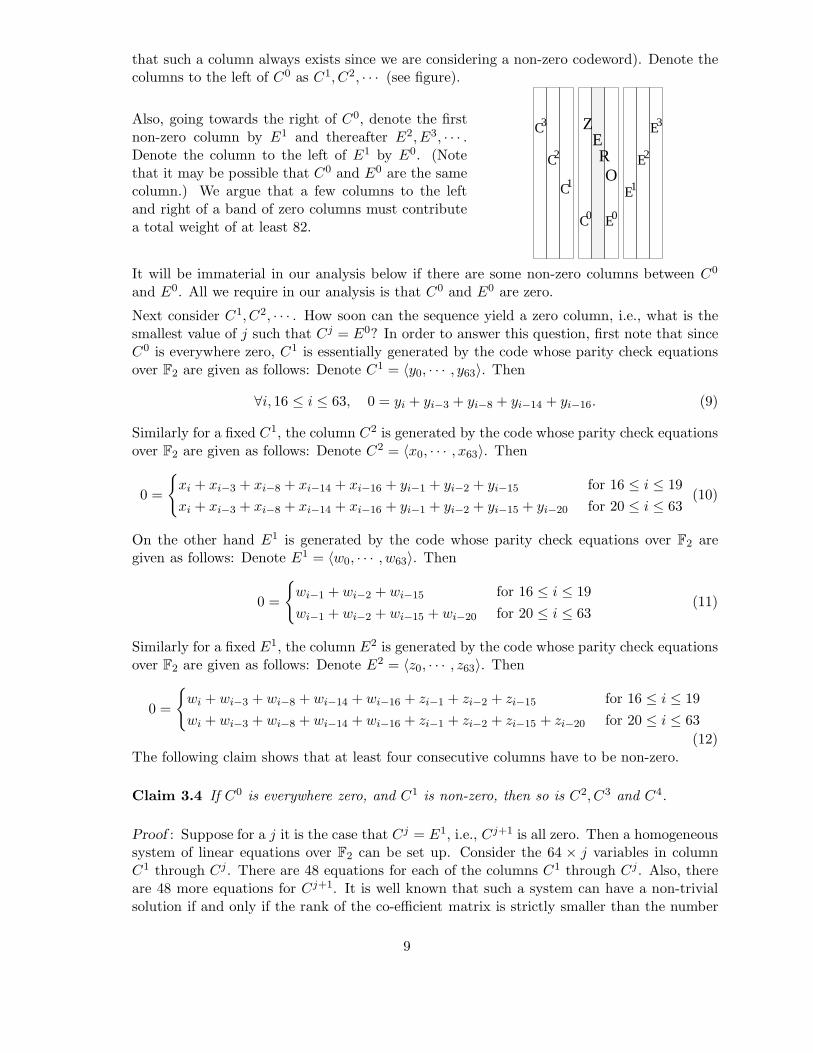
that such a column always exists since we are considering a non-zero codeword). Denote thecolumns to the left of C0 as C1, C2, · · · (see figure).

Also, going towards the right of C0, denote the firstnon-zero column by E1 and thereafter E2, E3, · · · .Denote the column to the left of E1 by E0. (Notethat it may be possible that C0 and E0 are the samecolumn.) We argue that a few columns to the leftand right of a band of zero columns must contributea total weight of at least 82.

O

C

C

C

2

3

1

0C

2E

E0

1E

E3ZER

It will be immaterial in our analysis below if there are some non-zero columns between C0

and E0. All we require in our analysis is that C0 and E0 are zero.

Next consider C1, C2, · · · . How soon can the sequence yield a zero column, i.e., what is thesmallest value of j such that Cj = E0? In order to answer this question, first note that sinceC0 is everywhere zero, C1 is essentially generated by the code whose parity check equationsover F2 are given as follows: Denote C1 = 〈y0, · · · , y63〉. Then

∀i, 16 ≤ i ≤ 63, 0 = yi + yi−3 + yi−8 + yi−14 + yi−16. (9)

Similarly for a fixed C1, the column C2 is generated by the code whose parity check equationsover F2 are given as follows: Denote C2 = 〈x0, · · · , x63〉. Then

0 =

{

xi + xi−3 + xi−8 + xi−14 + xi−16 + yi−1 + yi−2 + yi−15 for 16 ≤ i ≤ 19

xi + xi−3 + xi−8 + xi−14 + xi−16 + yi−1 + yi−2 + yi−15 + yi−20 for 20 ≤ i ≤ 63(10)

On the other hand E1 is generated by the code whose parity check equations over F2 aregiven as follows: Denote E1 = 〈w0, · · · , w63〉. Then

0 =

{

wi−1 + wi−2 + wi−15 for 16 ≤ i ≤ 19

wi−1 + wi−2 + wi−15 + wi−20 for 20 ≤ i ≤ 63(11)

Similarly for a fixed E1, the column E2 is generated by the code whose parity check equationsover F2 are given as follows: Denote E2 = 〈z0, · · · , z63〉. Then

0 =

{

wi + wi−3 + wi−8 + wi−14 + wi−16 + zi−1 + zi−2 + zi−15 for 16 ≤ i ≤ 19

wi + wi−3 + wi−8 + wi−14 + wi−16 + zi−1 + zi−2 + zi−15 + zi−20 for 20 ≤ i ≤ 63

(12)The following claim shows that at least four consecutive columns have to be non-zero.

Claim 3.4 If C0 is everywhere zero, and C1 is non-zero, then so is C2, C3 and C4.

Proof : Suppose for a j it is the case that Cj = E1, i.e., Cj+1 is all zero. Then a homogeneoussystem of linear equations over F2 can be set up. Consider the 64 × j variables in columnC1 through Cj. There are 48 equations for each of the columns C1 through Cj. Also, thereare 48 more equations for Cj+1. It is well known that such a system can have a non-trivialsolution if and only if the rank of the co-efficient matrix is strictly smaller than the number

9

of variables. It can easily be verified by a computer program that for j = 1, 2, 3, the systemhas full rank, that is exactly 64 × j. This can also be proved algebraically for j = 1, 2. Wegive a simple algebraic proof in the appendix (see Appendix A).This proof also highlights that for the rank to be full the recurrence relation must satisfy niceproperties. Ranks of all linear systems considered in this paper have been computed usingGaussian elimination. We now divide the proof into two cases.

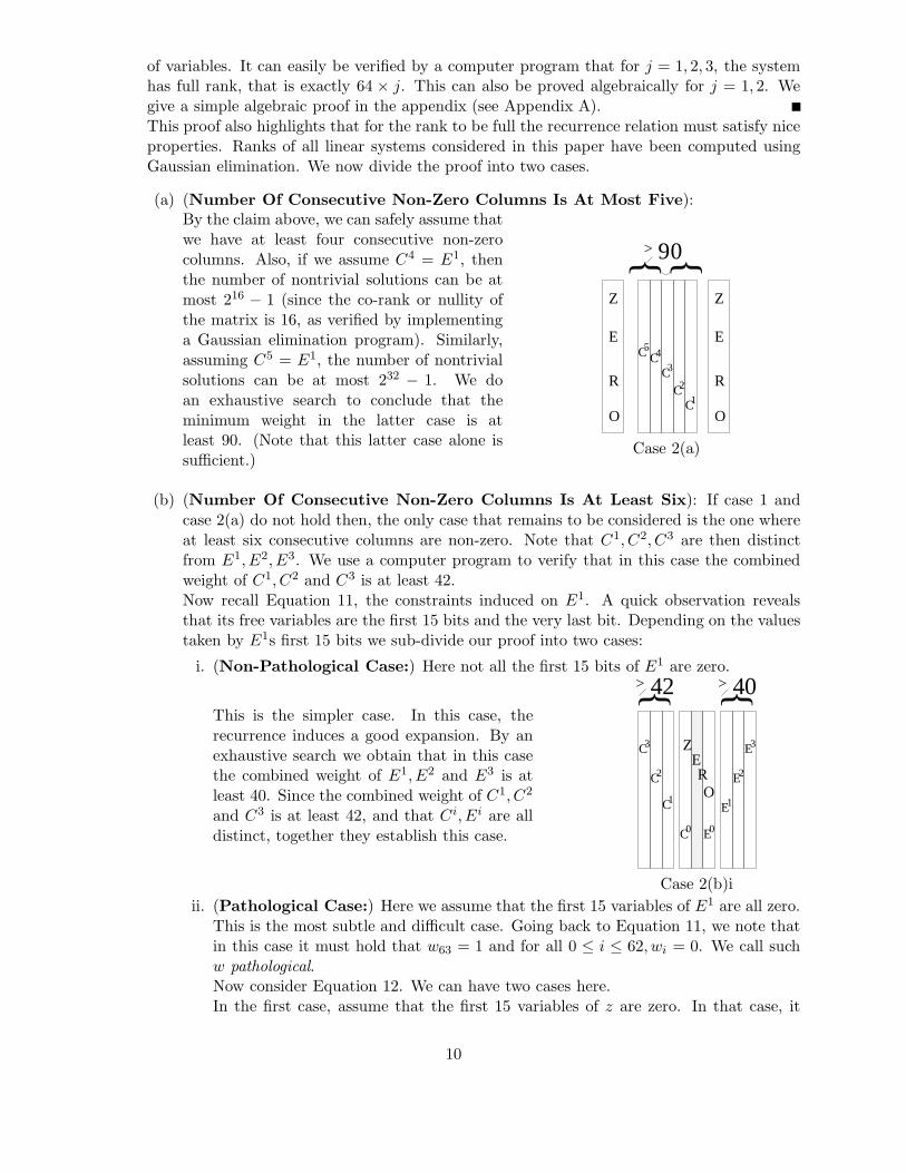
(a) (Number Of Consecutive Non-Zero Columns Is At Most Five):By the claim above, we can safely assume thatwe have at least four consecutive non-zerocolumns. Also, if we assume C4 = E1, thenthe number of nontrivial solutions can be atmost 216 − 1 (since the co-rank or nullity ofthe matrix is 16, as verified by implementinga Gaussian elimination program). Similarly,assuming C5 = E1, the number of nontrivialsolutions can be at most 232 − 1. We doan exhaustive search to conclude that theminimum weight in the latter case is atleast 90. (Note that this latter case alone issufficient.)

5

C

O

R

E

Z

}}

> 90

O

R

E

Z

C1C2

CC 43

Case 2(a)

(b) (Number Of Consecutive Non-Zero Columns Is At Least Six): If case 1 andcase 2(a) do not hold then, the only case that remains to be considered is the one whereat least six consecutive columns are non-zero. Note that C1, C2, C3 are then distinctfrom E1, E2, E3. We use a computer program to verify that in this case the combinedweight of C1, C2 and C3 is at least 42.Now recall Equation 11, the constraints induced on E1. A quick observation revealsthat its free variables are the first 15 bits and the very last bit. Depending on the valuestaken by E1s first 15 bits we sub-divide our proof into two cases:

i. (Non-Pathological Case:) Here not all the first 15 bits of E1 are zero.

This is the simpler case. In this case, therecurrence induces a good expansion. By anexhaustive search we obtain that in this casethe combined weight of E1, E2 and E3 is atleast 40. Since the combined weight of C1, C2

and C3 is at least 42, and that Ci, Ei are alldistinct, together they establish this case.

0

C

C

C

2

3

1

0C

2E

E0

1E

E3ZERO

}> 42 }> 4

Case 2(b)i

ii. (Pathological Case:) Here we assume that the first 15 variables of E1 are all zero.This is the most subtle and difficult case. Going back to Equation 11, we note thatin this case it must hold that w63 = 1 and for all 0 ≤ i ≤ 62, wi = 0. We call suchw pathological.Now consider Equation 12. We can have two cases here.In the first case, assume that the first 15 variables of z are zero. In that case, it

10

must hold that z62 = 1. (Plugging in i = 16 to 62 in Equation 12 will yield zj = 0for all 15 ≤ j ≤ 61 since wi = 0 for these values.) Also note that z63 is free. In thiscase, we also call z pathological. In fact this may continue along the diagonal i.e.,E3, E4, · · · may be pathological. If that happens then it is easy to show that thefirst non-zero bits of E3 will be its 61st bit, that of E4 will be 60th bit and so on.Also each column will have a free variable in its 63rd bit.In the second case, we assume that not all of its first 15 variables are zero. We callsuch z’s to be non-pathological.We now sub-divide into many small cases depending primarily on the number ofpathological columns (and thus on the number of free variables).

A. (# Pathological Columns ≤ 8) We break this case into two sub-cases. Thateach of these sub-cases holds has been verified using a computer program.

(I). 6th and earlier non-pathological columns are non-zero :

In this case, we verify that the combinedweight of the pathological columns andthe first three non-pathological columns tothe right of the pathological columns is atleast 40. This ensures that in this case theminimum weight is at least 82.

O

}}}

1E

<

R

E

Z

O

C

C

C

2

> 42

....E2

3

1

8#

> 40

ZE

R

}

Case 2(b)(ii)(A)(I)We mention that the search space dimension can be estimated as

# of Pathological variables + # of Non-Pathological Columns × 16,

which is at most 40 in this case.We next consider the case where the non-pathological columns are same as oneof C1, C2 or C3.

(II). 6th or earlier non-pathological column is identically zero: Firstly notethat it suffices to check the case where the 6th non-pathological column is iden-tically zero (that is E3 = C3), since other cases do fall in this case.Now we consider the parity check equationsinduced on the pathological columns andthe six non-pathological columns. Notethat C1 satisfies Equation 9 and that E1

satisfies Equation 11. Also note that inbetween columns satisfy equations similarto Equations 10 and 12. These equationsthen set up a homogeneous system of linearequations whose nullity can be verified (by acomputer program) to be at most 40.

O

}}

3C

E1 O

R

E

Z

<

C1C2

..E2

CC 45

O

R

E

Z

8#

8> 2

ZE

R

}

Case 2(b)(ii)(A)(II)Let the number of pathological columns be p and the number of non-pathologicalcolumns be n. Specifically then the nullity of the system can then be shown tobe exactly (see Appendix A Claim A.3)

p + 64 × n − 48 × (n + 1) = p + 16 · n − 48,

11

which is at most 40 in this case. We do an exhaustive search over the null spaceto establish that the min-weight is at least 82.

B. (8 < # Pathological Columns ≤ 16) We also break this case into two sub-cases. That each of these sub-cases holds has been verified using a computerprogram.

(I). 5th and earlier non-pathological columns are non-zero

In this case, we verify that the combinedweight of the pathological columns andthe first two non-pathological columns tothe right of the pathological columns is atleast 40. This ensures that in this case theminimum weight is at least 82.

O

8<#<16

} }}

E1

R

E

Z

O

C

C

C

2

> 42 }

3

1

> 40

..E2

ZE

R

Case 2(b)(ii)(B)(I)Therefore the case that remains to be considered is the one where the non-pathological columns are same as one of C2 or C3 which leads us to the nextcase.

(II). 5th or earlier non-pathological column is identically zero:

Firstly, note that it suffices to check thecase when the 5th non-pathological columnis identically zero (that is E2 = C3), sinceother cases do fall in this case. As in the2nd sub-case of the previous case (i.e., Case2(b)(ii)(A)(II)), we verify that the min-weightis at least 82.

O

} }

3C

E1 O

R

E

Z

8<#<16

C1C2

..E2

C4

O

R

E

Z

8> 2

ZE

R

}Case 2(b)(ii)(B)(II)

C. (16 < Pathological Columns ≤ 28) First of all, notice that 28 columns isenough, since by our assumption there is at least one zero column and threenon-pathological column (i.e., C1, C2, C3). Now, we also break this case intotwo sub-cases. That each of these sub-cases holds has been verified using acomputer program.

(I). 4th and earlier non-pathological columns are non-zero

12

In this case, we verify that the combinedweight of the pathological columns and thefirst non-pathological column to the right ofthe pathological columns is at least 40. Thisensures that in this case the minimum weightis at least 82.

O

}}

E1

R

E

Z

O

C

C2

> 42 }

..E2

3

C1

<16 #<28

> 40

ZE

R

}

Case 2(b)(ii)(C)(I)Therefore the case that remains to be considered is the one where the 1st non-pathological column is the same as C3.

(II). 4th non-pathological column is identically zero:

As in the 2nd sub-case of the previous case(or Case 2(b)(ii)(A)(II)), we verify that themin-weight is at least 82.

O

} }

E1O

R

E

Z

3C

..E2

<16 #<28

C1C2

8> 2

O

R

E

Z Z

RE

}

Case 2(b)(ii)(C)(II)

We remark that the minimum weight of this code can at most be 82 and therefore our resultis tight. We found the following codeword while searching for Case 2(b)(ii)(A)(II). Below we onlygive eight columns that includes six non-zero and two zero columns. The rests are all zero columns.Below the columns are placed horizontally.

0000000000000000 0000000000000000 0000000000000000 0000000000000000

0011110010011110 1000000001101001 1101001001010110 0000110010010000

1011000101000100 0010111101001000 1011100010101100 1101000000101111

1010101000111011 0010100100110010 1000000101001000 0110011000000000

0000000000000000 0000000000000000 0000000000000000 0000000000000100

0000000000000000 0000000000000000 0000000000000000 0000000000000011

0000000000000000 0000000000000000 0000000000000000 0000000000000001

0000000000000000 0000000000000000 0000000000000000 0000000000000000

3.3 The Last Sixty Words

In this subsection, we prove that the minimum weight of the code C in the last 60 words is atleast 75. In general, our proof strategy is robust, i.e., it can in principle be adapted to estimatethe minimum weight of this code in the last 4 · n (where n is an integer) number of steps, thoughthe dimension of the search space increases by an additive factor of (64 − 4 · n) and may make itcomputationally infeasible. On the other hand, when n gets smaller, say n ≤ 12, we may only need

13

to show an average 2 per column viz a viz Claim 3.3. Since most of our search is conducted usingearly-stopping, the large dimension is not expected to be a problem.

Next, observe that the minimum weight of the code C64 in the last 60 words yields a lower boundon the minimum weight of the code C in the last 60 words. Reviewing the proof of Theorem 3.2,it may be observed that in case 2 (i.e., At Least One Column Zero Case) we either consider acodeword (case 2(b)(ii)(A)(II), case 2(b)(ii)(B)(II) and case 2(b)(ii)(C)(II)) or consider few columns(in the remaining cases) which can always be extended to get a valid codeword. Therefore in thesecases just counting the weight of the last 60 words gives a lower bound on the minimum weightof the code in the last 60 words. However, the same is not true for case 1 (i.e., All Columns

Non-zero Case). We handle this case carefully. This then allows us to prove the followingtheorem.

Theorem 3.5 The code C64 , as defined by Equation 8, has minimum weight at least 75 in its last60 words.

Proof : Consider any column of length 64 bits. A column restricted to its bottom most 60 bits willhenceforth be referred to as a reduced column (see figure).

Unless otherwise mentioned, we will use the same name, eg., C0, todenote a column and its reduced column. We divide the proof intothree main cases.

0

olumn

column

rdcd.

4 bits

C

c

A Reduced Column

1. (All Columns Are Non-zero But Reduced Column Can Be Zero Case): Considerany such codeword. Also consider any non-zero column, w.l.o.g., let it be C0. Denote thecolumns, to the left of C0 by C1, C2, · · · , C31. Note that by assumption all columns arenon-zero.Then observe that due to this assumption notwo consecutive reduced columns can be zeroeverywhere. To see this let C0 and C1 be thecolumns such that their reduced columns areeverywhere zero. Let C1 be the column left toC0. Denote C0 by x = 〈x0, x1, · · · , x63〉 andC1 by y = 〈y0, y1, · · · , y63〉. Note that by theassumption xi = yi = 0 for all i = 4, · · · , 63.Now consider the parity check equations ofC64 and set i = 20.

0

4bits

60 bits

0

0

We gety20 + y17 + y12 + y6 + y4 + x19 + x18 + x5 + x0 = 0,

14

which implies x0 = 0. Similarly by setting i = 21, 22, 23, it can be seen that x is everywherezero.

We can therefore safely assume that no two consecutive reduced columns are zero. Then, thefollowing can be easily verified by a computer program.

Claim 3.6 For any non-zero column Ci, there exists k, 0 ≤ k ≤ 7 such that the combinedweight of the reduced columns Ci, Ci+1, · · · , Ci+k is at least 3 · (k + 1).

Note that although we restrict ourselves to at most 2 bits ON in reduced C0, we must considerall 16 possibilities for the first 4 bits of C0 to be able to define reduced column C1 (from16 bits in reduced column in C1 and all the bits in C0). Despite this the search is easilyconducted.

Then, following the same line of argument as in Case 1 (All Columns Non-Zero Case)of Theorem 3.2, it can be shown that the total weight of the reduced columns is at least 78.This is because 25 columns yield at least 75 and the remaining seven columns yield at least3 (since two consecutive reduced columns contribute at least 1).

2. (At Least One Column Zero Case): This case can be handled as the Zero Case in theproof of theorem 3.2. We consider the same number of cases and we count only the last 60bits in a column. We skip the details and summarize below the results we obtain.

(a) Number Of Consecutive Non-Zero Columns Is At Most Five:

The combined weight of the 5 non-zero col-umn is then at least 78.

8

C

O

R

E

Z

O

R

E

Z

}}C1

C2

CC 45

> 7

3

Case 3(a)

(b) Number Of Consecutive Non-Zero Columns Is At Least Six: The combinedweight of three reduced columns to the left of a zero band is at least 38.

i. (Non-Pathological Case) The combined weight of three reduced columns tothe right of a zero band is at least 38.

15

Therefore the combined weight of threereduced columns to the left of a zero columnand that of three reduced columns to theright of a zero column yields (assuming theyare distinct) at least 75.

7

C

C

C

2

3

1

0C

2E

E0

1E

E3ZERO

} }> >38 3

Case 3(b)(i)

ii. (Pathological Case)

A. # of Pathological columns ≤ 8

(I). 6th and earlier non-pathological columns are non-zero : The com-bined weight of the pathological reduced columns and the first three non-pathological reduced columns to the right of the pathological columns is atleast 37.

(II). 6th or earlier non-pathological column is zero: The combined mini-mum weight of these reduced columns is at least 75.

B. 8 < # of Pathological columns ≤ 16

(I). 5th and earlier non-pathological columns are non-zero : The com-bined weight of the pathological reduced columns and the first two non-pathological reduced columns to the right of the pathological columns is atleast 37.


C. 16 < # of Pathological columns ≤ 28

(I). 4th and earlier non-pathological columns are non-zero : The com-bined weight of the pathological reduced columns and the first non-pathologicalreduced columns to the right of the pathological columns is at least 37.


Therefore, in all these cases the combined weight of the reduced column is at least 75. This estab-lishes the theorem.

16

Z

}}}1E

<

C

C

C

2

>

....E2

3

1

8#

38 > 37

ER

O

Z

E

R

O

}

Case 2(b)(ii)(A)(I)

O

}}

E1

8<#<16

R

E

Z

O

C

C

C

2

> }

3

1

38 > 37

..E2

ZE

R

}

Case 2(b)(ii)(B)(I)

Z

}}

E1

R

E

Z

O

C

C2

> }

..E2

3

C1

<16 #<28

38 > 37

ER

O

}

Case 2(b)(ii)(C)(I)

O

}}

3C

E1

<

C1C2

..E2

CC 45

8#

> 75

ERO

ZZ

E

R

O

Z

E

R

}

Case 2(b)(ii)(A)(II)

} }

3C

E1 O

R

E

Z

8<#<16

C1C2

..E2

C4

O

R

E

Z

> 75

ZE

RO

}

Case 2(b)(ii)(B)(II)

E

} }

E1

3C

O

R

E

Z

..E2

<16 #<28

C1C2

> 75

O

R

E

Z Z

RO

}

Case 2(b)(ii)(C)(II)

Various Cases in the proof of Theorem 3.5(weights referred to the combined weights of the reduced columns)

Note that our result is tight. The codeword we cite in the previous subsection achieves thisbound.

3.4 The Last Forty-Eight Words

In this subsection, we prove that the code C64 has minimum weight at least 52 in its last 48 words.As mentioned previously, this proof is more computation intensive as the dimension of the searchspace increases by an additive factor of 16. The good thing is that we need to show an average 2per column, viz a viz Claim 3.3. This makes our search, conducted using early-stopping, feasiblein spite of the apparent large dimension.

It is easy to observe that the minimum weight of the code C64 in the last 48 words yieldsa lower bound on the minimum weight of the code C in the last 48 words. The proof uses thesame technique as in the proof of Theorem 3.5. Recall that in that proof (that is the proof ofTheorem 3.5) there are cases where we either consider a codeword or consider few columns whichcan always be extended to get a valid codeword. In those cases, just counting the weight of the last48 words suffices to give a lower bound on the minimum weight of the code in the last 48 words.In the remaining case, mimicking the proof of Theorem 3.5, we consider reduced columns (hererestricted to last 48 entries). We then can verify that under the assumption that all columns are

17

non-zero, the reduced columns cannot be too sparse. This then allows us to prove the followingtheorem.

Theorem 3.7 The code C64 as defined by Equation 8 has minimum weight at least 52 in its last48 words.

Proof : Consider any column of length 64 bits. Here a column restricted to its bottom most 48 bitswill henceforth be referred as a reduced column.Unless otherwise mentioned, we will use the same name, eg., C0, to denote a column and its reducedcolumn. We divide the proof into two main cases, depending on the existence of a zero column.

1. (All Columns Are Non-Zero But Reduced Column Can Be Zero Case ): Considerany such codeword. Also consider any non-zero reduced column, w.l.o.g., let it be C0. Denotethe reduced columns, to the left of C0 by C1, C2, · · · , C31. Note that if five consecutivereduced columns are zero, then the first column must be everywhere zero.

This is easily obtained by setting i suitablyin the parity check equations of the codeC64 (see figure). We handle that case latter.Therefore we can safely assume that no fiveconsecutive reduced columns are zero.

48 bits

4bits

00000

0000

000

00

0

Then the following is easily verified by a computer program.

Claim 3.8 For any non-zero column Ci, there exists k, 0 ≤ k ≤ 6 such that the combinedweight of the reduced columns Ci, Ci+1, · · · , Ci+k is at least (k+1). Furthermore, there existsℓ, 0 ≤ ℓ ≤ 8 such that the combined weight of the reduced columns Ci, Ci+1, · · · , Ci+ℓ is atleast 2 · (ℓ + 1).

Note that although we restrict ourselves to at most 1 bit ON in reduced C0, we must considerall 216 possibilities for the first 16 bits of C0 to be able to define reduced column C1 (from 16bits in reduced column in C1 and all the bits in C0). Since we rely heavily on early stopping,these bits must be guessed in a lazy fashion to make the search feasible. Then following thesame line of argument as in Case 1 (All Columns Non-Zero Case) of Theorem 3.5, it canbe shown that the total weight of the reduced columns is at least 53 (since 24 columns yieldat least 48 and the remaining eight columns yield at least 8, or 25 columns yield at least 50and the remaining 7 yields 7, or 26 columns yield 52 and remaining 6 at least 1).

2. At Least One Column Zero Case: In this case the first column must be everywhere zero.This case can then be handled as the Zero Case in the proof of theorem 3.2. We considerthe same number of cases and we count only the last 48 bits in a column. We remark that ineach such cases, it can be shown that the weight in the last 48 rounds is at least 52. We skipthe details.

18

4 Conclusion

4.1 Alternate codes

Notice that the code C64 has a sliding window of size 20, that is to encode a message using thiscode, an LFSR would require 20 registers. The following code has a sliding of size 17. This may beuseful for direct LFSR-type hardware implementation, since this would require three less registersthan what the code C64 requires.

Remark 4.1 We mention here that using our technique, it can be shown that the following codehas similar good minimum weight parameters as that of C64 .

Alternative1 :for i = 0, 1, · · · , 15, Wi = Mi andfor i = 16 to 63

Wi =

{



(13)

We expect the following code too to have equally good properties as the codes we have consid-ered/mentioned previously. However, because of additional pathological variables, the analysisbecomes more complex and we defer the complete analysis to a later time.

Remark 4.2 〈W0, · · · ,W79〉 are computed from the message 〈M0, · · · ,M15〉 as follows:

Alternative2 :for i = 0, 1, · · · , 15, Wi = Mi andfor i = 16 to 63

Wi = Wi−3 ⊕ Wi−8 ⊕ Wi−14 ⊕ Wi−16 ⊕ ((Wi−1 ⊕ Wi−2 ⊕ Wi−11 ⊕ Wi−15) <<< 1)

⊕ ((Wi−1 ⊕ Wi−2 ⊕ Wi−11 ⊕ Wi−15) >>> 1) (14)

4.2 Our proposed code vs. SHA-256 code

The code in SHA-256 ([Uni02]) is the following: Let 〈W0, · · · ,W15〉 be the 512 bits input to SHA-256, where each Wi is a word of 32 bits. Then the message expansion phase outputs 〈W0, · · · ,W63〉where

∀i, 16 ≤ i ≤ 63, Wi = σ1(Wi−2) + Wi−7 + σ0(Wi−15) + Wi−16, (15)

where σ0 and σ1 are as follows:

σ0(x)def= (x >>> 7) ⊕ (x >>> 18) ⊕ (x >> 3).

19

σ1(x)def= (x >>> 17) ⊕ (x >>> 19) ⊕ (x >> 10);

In the above, “>> i” denotes a right shift by i bit and ‘+’ denotes binary addition modulo 232.Note that the binary addition makes the code non-linear. We do not see how to lower bound theminimum weight of the above code. In spite of the complex description, we do not know how toformally argue about the security that this code offers.

One property that the SHA-256 code has which might be useful against [CJ98] and [WYY05b]attacks is that the code is not quasi-cyclic. These attacks require that a codeword rotated (alongcolumns) is again a codeword. Similarly, the attacks require that the codewords shifted (alongrows) is again a codeword. In fact, even our proposed code, although quasi-cyclic, is not invariantunder shifts along rows. This is because the recurrence relation changes from step 36 onwards.However, claiming security on this basis maybe short-lived, and arguably there is no substitute toactually proving that the code has a high minimum weight.

4.3 Modifying SHA-256

It should be noted that SHA-256, unlike SHA-1, has only 64 steps. There are two reasons whythe designers of SHA-256 probably considered it safe to reduce the number of steps: firstly, sinceSHA-256 produces a 128 bit output, its non-linear block cipher has eight 32 bit registers instead ofthe five that SHA-1 has. This in turn means that any disturbance introduced using the expandedmessage words Wi carries on for at least eight rounds (instead of five), and hence the probabilityof forcing local collisions goes down. Secondly, the SHA-256 message expansion code itself is moreinvolved and possibly has better minimum distance (though as discussed in the previous subsection,there is no proof of that).

Utilizing the first observation, we believe that a provably good message expansion into 64 wordsdoes indeed render the “modified” SHA-256 secure against differential attacks. For the code wecan use a back truncation of the code C analyzed in this paper, i.e. given by equation (2) but withi <= 63. Of course, one would need to analyze this code from scratch, as the minimum weightnumbers for the code C do not automatically yield numbers for the back truncation.

Another interesting code, which we plan to analyze in the future, is a code similar to Alternative2 above but with a sliding window of size 20. Recall (see the last para of section 3.1) that increasingthe window size allows us to get rid of certain pathological variables, and makes the search feasible.Moreover, it also simplifies the analysis considerably. In particular, the code we plan to analyzeand recommend for SHA-256 is:

Wi =

Wi−3 ⊕ Wi−8 ⊕ Wi−14 ⊕ Wi−16

⊕((Wi−1 ⊕ Wi−2 ⊕ Wi−15) <<< 13)

⊕((Wi−1 ⊕ Wi−2 ⊕ Wi−15) >>> 13) if 16 ≤ i < 36

Wi−3 ⊕ Wi−8 ⊕ Wi−14 ⊕ Wi−16

⊕((Wi−1 ⊕ Wi−2 ⊕ Wi−15) <<< 13)

⊕((Wi−1 ⊕ Wi−2 ⊕ Wi−15 ⊕ Wi−20) >>> 13) if 36 ≤ i ≤ 63

(16)

As before, we would need to lower bound its minimum weight in the last 48 (and possibly last

20

32) words. One crucial observation we make is that in analyzing C, we could estimate the dimensionof the subspace such that C5 = E1 (see case 2(a) in the proof of Theorem 3.2) to be about 32(in fact exactly 32). This follows by just observing the number of variables, and the homogeneousequations involved. However, when the length of the code is reduced as above, this subspace hasdimension at least 48. But, by mixing three columns at a time as in the above code, the numberof equations in that case (i.e., in case 2(a) in the proof of Theorem 3.2) goes up considerably, andthe null space has a more reasonable dimension of about 16.

4.4 Acknowledgment

We thank Pankaj Rohatgi for motivating us throughout this work, and particularly for his insightfulcomments on an earlier version of this manuscript. We also thank W. Eric Hall for providing uswith the hardware estimates, and Ronald Rivest for suggesting the name SHA1-IME. The secondauthor also wishes to thank Alexandar Vardy and Patrick Sole for helpful suggestions.

References

[BC04a] E. Biham and R. Chen. Near collisions of SHA-0. In Crypto, 2004.

[BC04b] E. Biham and R. Chen. New results on SHA-0 and SHA-1. In Short talk presented atCRYPTO’04 Rump Session, 2004.

[Che92] V. V. Chepyzhov. New lower bounds for minimum distance of linear quasi-cyclic andalmost linear cyclic codes. In Problems of information Transmission, Vol. 28, No. 1,1992.

[CJ98] F. Chabaud and A. Joux. Differential collisions in SHA-0. In Crypto, 1998.

[DMS03] I. Dumer, D. Micciancio, and M. Sudan. Hardness of approximating the minimumdistance of a linear code. In IEEE Transaction on Information Theory, 49(1), 2003.

[Lal03] K. Lally. Quasicyclic codes of index ℓ over Fq Viewed as Fq[x]-submodules ofFql [x]/〈xm − 1〉. In Lecture Notes in Computer Science, Vol. 2643, Springer, 2003.

[LS05] Ling and P. Sole. Structure of quasi-clcyic codes III: Generator theory. In IEEETransaction on Information Theory, 2005.

[MP05] K. Matusiewicz and J. Pieprzyk. Finding good differential patterns for attacks onSHA-1. In International Workshop on Coding and Cryptography, 2005.

[Riv92] R. Rivest. RFC1321: The MD5 message-digest algorithm. In Internet Activities Board,1992.

[RO05] V. Rijmen and E. Oswald. Update on SHA-1. In Lecture Notes in Computer Science,Vol. 3376, Springer, 2005.

[TW67] R. L. Townsend and E. J. Weldon. Self-orthogonal quasi-cyclic codes. In IEEE Trans-action on Information Theory, 1967.

21

[Uni93] United States Department of Commerce, National Institute of Standards and Technol-ogy, Federal Information Processing Standard Publication #180. Secure Hash Standard,1993.

[Uni95] United States Department of Commerce, National Institute of Standards and Tech-nology, Federal Information Processing Standard Publication #180-1 (addendum to[Uni93]). Secure Hash Standard, 1995.

[Uni02] United States Department of Commerce, National Institute of Standards and Tech-nology, Federal Information Processing Standard Publication #180-2. Secure HashStandard, August, 2002.

[Var97] A. Vardy. The intractability of computing the minimum distance of a code. In IEEETransaction on Information Theory, 43(6), 1997.

[WYY05a] X. Wang, H. Yu, and Y. L. Yin. Efficient collision search attacks in SHA-0. In Crypto,2005.

[WYY05b] X. Wang, H. Yu, and Y. L. Yin. Finding collisions in the full SHA-1. In Crypto, 2005.

A Rank proofs

Claim A.1 If C0 is zero, and C1 is non-zero, then C2 is non-zero.

Proof : Assume otherwise i.e., that C2 is zero. Consider the following 48 × 64 dimensional paritycheck matrices (essentially Equations 9 and 11) over F2

1010000010000100100000 · · · 0000000000000000000101000001000010010000 · · · 000000000000000000

. . . · · ·. . .

0000000000000000000000 · · · 010100000100001001

H1

0100000000000011000000 · · · 0000000000000000000000010000000000001100000 · · · 0000000000000000000000001000000000000110000 · · · 0000000000000000000000000100000000000011000 · · · 000000000000000000000

1000010000000000001100 · · · 0000000000000000000000100001000000000000110 · · · 000000000000000000000

. . . · · ·. . .

0000000000000000000000 · · · 100001000000000000110

H2

22

Then we need to show that H =

(

H1

H2

)

has full rank. To do that it is enough to show that

there are 64 linearly independent rows. We consider the 48 rows of H1 and 16 additional rows,namely 5th through 20th rows of H2. We reduce the problem to showing that a certain equationover polynomial ring F2[x] does not have solutions in a restricted set of polynomials. We associatewith the vector c = 〈c0, · · · , c63〉 in F64

2 the polynomial c(s) =∑

63

i=0cis

i in F2[s]. Then the followingpolynomials can be associated with the 1st and 5th rows of matrix H1 and H2, respectively:

p(s)def= s16 + s13 + s8 + s2 + 1,

r(s)def= s19 + s18 + s5 + 1.

Further note that the ith (note 1 ≤ i ≤ 48) row of H1 then gets associated with si−1p(s). Similarlythe jth (note we restrict ourselves to 5 ≤ j ≤ 20) row of H2 then gets associated with sj−5r(s).Therefore, observe that if the 80 rows that we are considering were dependent then we can translatethat to a non-zero solution of the following polynomial equation:

p(s)α(s) + β(s)r(s) = 0,

with additional constraints that degree(α) ≤ 47 and degree(β) ≤ 15. However, it is well knownthat p(s) is irreducible, therefore if such a equation holds then it must be the case that p(s) dividesr(s). However, it is easy to check that p(s) does not divide r(s), thus leading to a contradiction.Therefore H has full rank.

Claim A.2 If C0 is zero, and C1 is non-zero, then C2, C3 is non-zero.

Proof : Consider the following polynomials :

p(x)def= x16 + x13 + x8 + x2 + 1,

q(x)def= x15 + x14 + x,

r(x)def= x19 + x18 + x5 + 1 = x4 · q(x) + 1.

Let H1 and H2 be as above.

First of all note that H2 has full rank. (This is clear from the matrix. Otherwise, note that wecould have an identity

q(x) · a(x) + r(x) · b(x) = 0

with degree(a) ≤ 3 and degree(b) ≤ 43. Since degree(q · a) < degree(r), this cannot happen.) Nowwe will show that the rank of the matrix

H2 0H1 H2

0 H1

is at least 128. Since H1 has full rank, observe that

(

H1 H2

0 H1

)

23

has rank at least 96. So consider the following 92 independent rows from the above matrix, namely5th row onwards. We also argue that another additional 5th through 40th rows of the top H2 arealso independent. If not, then they would satisfy the following polynomial equations

α(x)p(x) + β(x)r(x) = 0 (17)

x4β(x)p(x) + γ(x)r(x) = 0 (18)

with restrictionsdegree(α) ≤ 47,degree(β) ≤ 43, anddegree(γ) ≤ 35.

Since p(x) is an irreducible polynomial, and p(x) ∤ r(x), observe from Equation 17 that p(x)|β(x).Hence, set β(x) = µ(x)p(x). Substituting in Equation 18 we get

x4p(x)2µ(x) + γ(x)r(x) = 0.

Since p(x) is irreducible, and p(x) ∤ r(x), and x ∤ r(x), it must hold that x4p(x)2|γ(x). But that isimpossible, since degree(γ) ≤ 35 < 36 =degree(x4p(x)2).

Recall that we used E0 to denote a column that is zero everywhere. Also, recall that the columnsleft to E0 are denoted E1, E2 and so on. In the following claim, we will assume 3 ≤ n.

Claim A.3 Let E1, E2, · · · , Ep be p pathological columns. Also, let Ep+1, Ep+2, · · · , Ep+n be nnon-pathological columns. Further assume that Ep+n+1 = C0 is everywhere zero. If the nullity ofthe parity check equations resulting from these columns with p = 0 is 16 ·n− 48, then the nullity ofthe parity check equations resulting from these columns with any p ≤ 28 is

p + 16 · n − 48.

Proof : Let Ni,j, (1 ≤ i ≤ n, 0 ≤ j ≤ 63) denote the entries in the non-pathological columns. Alsolet Pi,j , (1 ≤ i ≤ p, for each i, 64 − i ≥ j ≤ 63) be the pathological variables. We will denoteNi = 〈Ni,0, · · · , Ni,63〉 and Pi = 〈Pi,64−i, · · · , Pi,63〉. Let H1|i denote the matrix H1 restricted to thelast i columns. (Note that only the last i rows will be non-zero.) Also let H2|i denote the matrixH2 restricted to the last i columns. (Note that only the last i−1 rows will be non-zero.) Note that〈P1, · · · , Pp, N1, · · · , Nn〉 must belong to the null space of the following matrix:

H =

H1|1 H2|2

H1|2 H2|3

. . .. . .

H1|p−1 H2|p

H1|p H2

H1 H2

. . .. . .

H1 H2

H1

Note that when we restrict H1 or H2 to the last few columns, the top rows in that restrictedentries may become zero row. We remove such rows if the entire row in the above matrix Hbecomes everywhere zero. Note that with this modification, the following sub-matrix is already inthe echelon form:

H1 =

H1|1 H2|2

H1|2 H2|3

. . .. . .

H1|p−1 H2|p

(p − 1) blocks

24

(Observe that first block corresponding to (H1|1 H2|2) reduces to (1 10), and that corresponding to

(H1|2 H2|3) reduces to

(

10 10001 110

)

.)

Furthermore, since by assumption the following sub-matrix has full rank:

H2 =

H2

H1 H2

. . .. . .

H1 H2

H1

(n + 1) blocks

the matrix H has full rank. Note here that in the top 48 − p rows, H1|p is entirely zero. Howeverthese rows in H are independent since H2 has full rank. In the remaining rows H1|p is in echelonform and hence independent. Note that it has number of rows i.e., constraints:

48 × (n + 1) +

p−1∑

i=1

i = 48(n + 1) +p(p − 1)

2.

Also, note the number of variables i.e., columns is

64 × n +

p∑

i=1

i = 64 · n +p(p + 1)

2.

Thus the nullity of the system is

64 · n +p(p + 1)

2−

(

48(n + 1) +p(p − 1)

2

)

= p + 16 · n − 48.

This completes the proof.

B Examples

We cite below an example where over 7 columns an average of 3 does not hold. Below we only give8 columns and the columns are placed horizontally. Note that the 8 columns yield 29, whereas thefirst 7 columns yield only 14.

0000000000000000000000000000000000000000000000000000000001000000

0000000000000000000000000000000000000000000000000000000000110110

0000000000000000000000000000000000000000000000000000000000010100

0000000000000000000000000000000000000000000000000000000000001110

0000000000000000000000000000000000000000000000000000000000000100

0000000000000000000000000000000000000000000000000000000000000011

0000000000000000000000000000000000000000000000000000000000000001

1000101010000000001001000010000010000100101100000010001000010000

25

Documents

A Simple and Provably Good Code for SHA Message Expansion