A RECURRENT NEURAL FILTER FOR ADAPTIVE NOISE CANCELLATION

Paris A. Mastorocostas, Dimitris N. Varsamis, Constantinos A. Mastorocostas, Constantinos S. Hilas

Department of Informatics & Communications, Technological Educational Institute of Serres 62124, Serres

Greece mast@teiser.gr, dvarsam@teiser.gr, costas_mast@teiser.gr, chilas@teiser.gr

ABSTRACT This paper presents a dynamic neural filter for adaptive noise cancellation. The cancellation task is transformed to a system-identification problem, which is tackled by use of the Block-Diagonal Recurrent Neural Network. The filter is applied to a benchmark noise cancellation problem, where a comparative analysis with a series of other dynamic models is conducted, underlining the effectiveness of the proposed filter and its superior performance over its competing rivals. KEY WORDS block-diagonal recurrent networks, adaptive noise cancellation 1. Introduction Extraction of an information signal buried in noise is one of the benchmark problems in the area of signal processing [1]. The issue of noise cancellation is encountered in many cases, including interference in electrocardiographs and periodic interference in speech signals. The most common method of signal estimation is to pass the noisy signal through a filter, which tends to suppress the noise while leaving the signal relatively unchanged. The filters applied to this problem are fixed or adaptive. The design of the former is based on prior knowledge of both the signal and the noise. Adaptive filters, on the other hand, have the ability to adjust their parameters automatically, requiring little or no prior knowledge of the signal or noise characteristics. The problem of adaptive noise cancellation has been widely studied during the last decades and there exists a variety of filters in literature. Recently, neural networks have been employed to this area, exhibiting promising results [2]-[3]. In all cases, however, the suggested structures are static and the series-parallel identification approach is followed. Therefore, these models provide insufficient signal estimations when noise passes through nonlinear dynamic channels. In an attempt to alleviate this problem, a number of recurrent neural and fuzzy-neural models have been suggested as dynamic adaptive noise cancellers [4]-[6].

These models are capable of effectively model the dynamics of a channel and exhibit superior cancellation performance compared to the aforementioned static neural models. In this work an alternative recurrent structure is proposed as a noise cancellation filter. The filter is implemented by the Block-Diagonal Recurrent Neural Network [7], which has been proved in [8] to be an efficient identification tool. The rest of paper is organized as follows: In Section 2 the transformation of the noise cancellation problem to a system identification problem is given. In the next section the proposed model is briefly described. Finally, Section 4 hosts the simulation results, where a comparative analysis with other recurrent neural and fuzzy models is conducted.

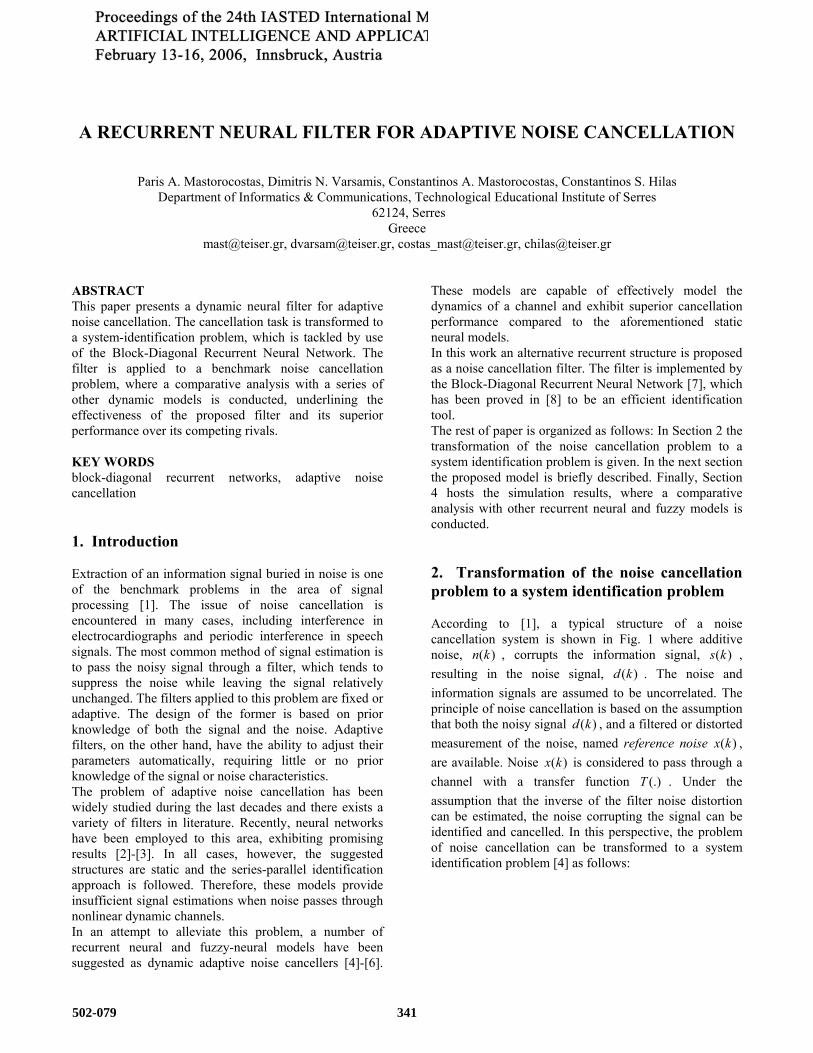
2. Transformation of the noise cancellation problem to a system identification problem According to [1], a typical structure of a noise cancellation system is shown in Fig. 1 where additive noise, , corrupts the information signal, s , resulting in the noise signal, d . The noise and information signals are assumed to be uncorrelated. The principle of noise cancellation is based on the assumption that both the noisy signal , and a filtered or distorted measurement of the noise, named reference noise x , are available. Noise x is considered to pass through a channel with a transfer function T . Under the assumption that the inverse of the filter noise distortion can be estimated, the noise corrupting the signal can be identified and cancelled. In this perspective, the problem of noise cancellation can be transformed to a system identification problem [4] as follows:

)(kn )(k

)(k

)(k

)(kd

)(k(.)

502-079 341

Ó

Ón k( )

s k( )

d k( )

x k( )

$( )y k

e k( )

T (. ) F(. )

adaptive noise canceller

Filter

Fig. 1. The problem of adaptive noise cancellation

3. The proposed network and the modeling method As shown in the previous section, the noise cancellation problem can be handled as a system identification problem. In this perspective, the model employed to perform system identification is the Block-Diagonal Recurrent Neural Network (BDRNN) [7]. The Block-Diagonal Recurrent Neural Network is a two-layer network, with the output layer being static and the hidden layer being dynamic. The hidden layer consists of pairs of neurons (blocks); there are feedback connections between the neurons of each pair, introducing dynamics to the network.

d k( )

Óx k( )

$( )y k

e k( )

F(. )

ÓT −1(. )n k( )

s k( )non-accesible part

Filter

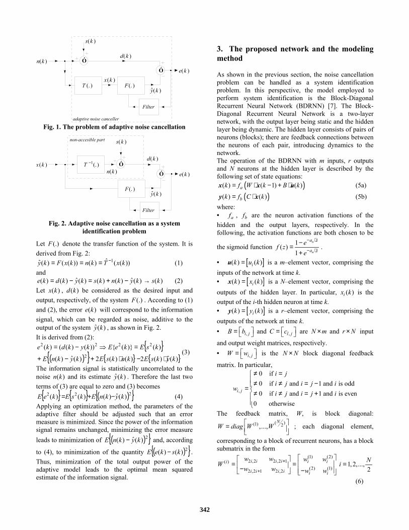
Fig. 2. Adaptive noise cancellation as a system identification problem

The operation of the BDRNN with m inputs, r outputs and N neurons at the hidden layer is described by the following set of state equations:

(( ) ( 1) ( )ak f W k B k= ⋅ − + ⋅x x u ))

(5a)

(( ) ( )bk f C k= ⋅y x (5b) where: • , are the neuron activation functions of the hidden and the output layers, respectively. In the following, the activation functions are both chosen to be

the sigmoid function

af bf

1( )1

n

n

a z

a zef ze

− ⋅

− ⋅−=+

.

Let denote the transfer function of the system. It is derived from Fig. 2:

(.)F

• [ ]( ) ( )ik u k=u is a m–element vector, comprising the inputs of the network at time k.

))((ˆ)())(()(ˆ 1 kxTknkxFky −=== (1) and

• [ ]( ) ( )ik x k=x is a N–element vector, comprising the outputs of the hidden layer. In particular, ( )ix k is the output of the i-th hidden neuron at time k.

)()(ˆ)()()(ˆ)()( kskyknkskykdke →−+=−= (2) Let , be considered as the desired input and output, respectively, of the system . According to (1) and (2), the error will correspond to the information signal, which can be regarded as noise, additive to the output of the system , as shown in Fig. 2.

)(kx )(kd(.)F

)(ke

(y )k

• [ ]( ) ( )ik y k=y is a r–element vector, comprising the outputs of the network at time k. • ,i jB b = and ,l jC c = are and input

and output weight matrices, respectively.

N m× r N×It is derived from (2):

{ }( ){ } { } { })(ˆ)(2)()(2)(ˆ)(

)()}({))()(()(2

2222

kyksEknksEkyknE

ksEkeEkykdke

⋅−⋅+−+

=⇒−=(3) • ,i jW w = is the block diagonal feedback

matrix. In particular,

N N×

The information signal is statistically uncorrelated to the noise and its estimate y . Therefore the last two ter zero and (3 becomes

)(kn )(ˆ k

,

0 if 0 if and 1 and is odd0 if and 1 and is even

0 otherwise

i j

i ji j i j i

wi j i j i

≠ =≠ ≠ = −= ≠ ≠ = +

ms of (3) are equal to )){ } { } ({ }222 )(ˆ)()()( kyknEksEkeE −+= (4)

Applying an optimization method, the parameters of the adaptive filter should be adjusted such that an error measure is minimized. Since the power of the information signal remains unchanged, minimizing th error measure leads to minimization of

e)({ }2)(ˆ)( kyknE − and, according

to (4), to minimization of the quantity ( ){ }2)()( kske −E . Thus, minimization of the total output power of the adaptive model leads to the optimal mean squared estimate of the information signal.

The feedback matrix, W, is block diagonal: ( )(1) 2,...,N

W diag W W = ; each diagonal element,

corresponding to a block of recurrent neurons, has a block submatrix in the form

(1) (2)2 ,2 2 ,2 1( )

(2) (1)2 ,2 1 2 ,2

i i i i i ii

i i i i i i

w w w wW

w w w w+

+

= = − −

1,2,...,2Ni =

(6)

342

Equation (6) describes a special case of BDRNN, which has scaled orthogonal sub-matrices. As shown in the literature, this network exhibits superior modelling capabilities over other forms of BDRNN. In view of the above, the state equations (5) for the Scaled Orthogonal BDRNN can take the following form:

(1)2 1 2 1, 2 1

1

(2)2

( ) ( ( ) ( 1)

( 1)), 1,...,2

m

i a i j j i ij

i i

x k f b u k w x k

Nw x k i

− − −=

= ⋅ + ⋅

+ ⋅ − =

∑ − (7a)

(2)2 2 , 2 1

1

(1)2

( ) ( ( ) ( 1)

( 1)), 1,...,2

m

i a i j j i ij

i i

x k f b u k w x k

Nw x k i

−=

= ⋅ − ⋅

+ ⋅ − =

∑ −

r

(7b)

,1

( ) ( ( )), l 1,...,N

l b l j jj

y k f c x k r=

= ⋅ =∑ 1,...,l = (7c)

where , are the feedback weights at the hidden

layer.

(1)iw (2)

iw

The BDRNN is trained by the RENNCOM algorithm. The algorithm, entitled Recurrent Neural Network Constrained Optimization Method is fully described in [8] and a brief description is given in the sequel. The training method aims at transforming the learning process to a constrained optimization problem, which has been solved using methods based on optimal control theory and the calculus of variations. For the case of a -input- -output BDRNN with scaled orthogonal feedback submatrices, the objective of the learning process is to adjust the network parameters so that a prescribed input/output mapping is captured. Learning is carried out in a parallel mode using a data batch

mr

( ){ }ˆ( ( ) , 1,...,), fk k k k=u y comprising fk input-output

pairs. Two vectors are introduced: a) the state vector ( )st t , defined as:

[ 1 1( ) ( ),..., ( ), ( ),..., ( ) TN rk x k x k y k y k=st ] (8)

comprising the outputs of the hidden and the output layer. b) the control vector comprising the synaptic and feedback weights

θ

(1) (1) (2) (2)1,1 , 1,1 ,1 1

2 2

,..., , , , , , ,...,

T

N m r NN Nb b w w w w c c =

θ (9)

For a data set including fk pairs, the state equations (7)

are written ( ) , 1,..., f(k), (k) k k= =f st θ 0 (10)

(1) (2)2 1, 2 1 2

1( ) ( 1) ( 1)

m

a i j j i i i ij

f b u k w x k w x k− −=

+ − + ∑ −

=

−

r

(2) (1)2 , 2 1 2

1( ) ( 1) ( 1)

m

a i j j i i i ij

f b u k w x k w x k−=

− − + ∑

2 ( ) 0ix k− = (11b)

,1

( ) ( ) 0N

b l j j lj

f c x k y k=

− = ∑ ( equations) (11c) fk ×

The suggested algorithm is an iterative procedure which aims at achieving two objectives, simultaneously: • It is desired that an error measure function, E, should be minimized, in order to perform the input-output mapping, successfully. The Mean Squared Error (MSE) is selected here and is defined by

2

1 1

1 ˆ( ) ( )fk r

l lf k l

E y k yk = =

= − k ∑∑ (12)

where is the l-th model output, y k is the l-th desired (actual) output of the system at time step k.

( )ly k ˆ ( )l

• Secondly, a nonlinear multivariable function , called the pay-off function, should be optimized. In the present case the main scope is to facilitate and accelerate the learning process. The following pay-off function is selected:

Φ

( ) (Tcur cur prevΦ = − −θ θ θ θ )

dθ

(13)

where , are the control vectors at the current

and the previous epochs, respectively. Maximization of the pay-off function at each epoch implies that the current and previous weight updates are highly aligned, thus avoiding zig-zag trajectories and improving the convergence speed .

curθ prevθ

Optimization of (12) and (13) is iteratively performed with respect to the decision variables, θ and the state variables, , under the architectural constraints imposed by the state equations (11). In that sense, the learning process can be regarded as a constrained optimization problem.

st

Following the procedure dictated in [8], the weights are updated as follows, with t being the epoch index:

( 1) ( )t t+ = +θ θ (14) The corrective vector is given by: dθ

( )2

2( ) T2 TEE E

EEEEE E

I E Id ∆II I I

δ ΦΦ

ΦΦ Φ

−= − ⋅ ⋅ − ⋅ ⋅ − θ Λ Λ

( )T2E

EE

E∆Iδ+ ⋅ ⋅Λ (15)

where the following factors are calculated: 2

EE E EI Τ= ∆Λ Λ2

EI ΤΦ Φ= ∆Λ Λ

(16a) (16b)

(16c)

2I ΤΦΦ Φ Φ= ∆Λ Λ

E EEIE ⋅−= ξδ (16d) and ξ is a constant over [0,1].

2 1( ) 0ix k−− (11a)

343

The intermediate variables TΦ

Φ∂ = ∂ θ

Λ and

TT

E∂= ⋅ ∂

fθ

Λ λ are calculated by use of the Lagrange

multipliers, which are given by:

0TE∂ ∂∂ ∂

+ ⋅ =fst st

λ (17)

Matrix is the

Maximum Parameter Changes matrix (MPC). At each epoch the weights are changed by small amounts d , so that the positive quadratic equation holds:

1 2 ( 1)( , , . . ., )N m r∆ diag ∆ ∆ ∆ × + +=

θ

2

1

( )1

ni2

i i

d∆θ

==∑ or (18) 1( ) 1T 2d ∆ d− =θ θ

where is the MPC for i∆ iθ . Equation (18) describes a

hyper-ellipsoid centered at the point defined by the current control vector, whose axes are the i∆ ’s. Since the

search space is defined in terms of , the MPC’s play an essential role in the learning process and is desired to be adaptable throughout the learning process. The adaptation mechanism is fully described in [8].

i∆

Summarizing, at each epoch t the RENNCOM algorithm proceeds as follows: First, the current values of

’s are derived according to the suggested adaptation schedule. Next, parameter learning is performed, by calculating the optimal parameter changes. If the resulting error measure is smaller than a prescribed threshold, learning is completed, otherwise the whole process is repeated.

=1 2, ,....

i∆

4. Simulation Results In this section the proposed filter is applied to a noise cancellation problem, where the noise n passes through a nonlinear dynamic channel, producing the reference noise x(k). The passage’s dynamics is simulated by a second order nonlinear auto-regressive model with exogenous inputs (NARX) [4]:

)(k

2( ) 0.25 ( 1) 0.1 ( 2) 0.5 ( 1) 0.1 ( 2)

0.2 ( 3) 0.1 ( 2) 0.08 ( 2) ( 1)x k x k x k n k n k

n k n k n k x k= − + − + − + −− − + − + − − (19)

The information signal s is a saw-tooth signal of unit magnitude, 50 samples period, as shown in Fig. 3a. The signal is corrupted by a uniformly distributed white noise sequence varying in the range [ shown in Fig. 3b while the noise-corrupted signal d is depicted in Fig. 3c. The training data sets consist of 12000 pairs

, while the testing set comprises 1000 data pairs.

)(k

)(ks

)(kd

]2,2−)(k

[ ),(kx ]

The BDRNN comprises eights blocks of neurons in the hidden layer. Training lasts for 1000 epochs. The learning

parameters of the RENNCOM algorithm are shown in Table 1. A time section of eight periods of the recovered signal is presented in Fig.3d. It is evident that even though the information signal has half the amplitude of the additive noise, the former is accurately identified, with the exception of a few high frequency components.

Table 1 The learning parameters of the RENNCOM method

na n+ n− 0∆ ξ

2 1.05 0.95 1E-2 0.9 In the sequel, a comparative analysis is attempted between the suggested BDRNN filter and a class of noise cancellation filters including finite impulse response (FIR) and infinite impulse response (IIR) neural networks and a fuzzy inference system: • A Dynamic Fuzzy Neural Network (DFNN), taken from [6]. • A recurrent three-layer neural network (FIRN), in the form of 1- H -1, having a linear input layer, and FIR synapses at the hidden and output layers, as described in [6]. The outputs of the hidden and output layers are given by the following formulas:

[ ]

+−= ∑

=

3

0

11 )(tanh)( i

Ou

qqii wqkuwkO (20a) Hi ,...,1=

[ ]

+−= ∑∑

= =

6

1 0

14 )(tanh)( wqkOwkyH

j

Oy

qjqj (20b)

• A recurrent three-layer neural network (IIRN), in the form of 1- H -1, having a linear input layer, and Frasconi-Gori-Soda [9] neurons in the hidden and output layers. The outputs of these neurons are determined by the following formulas:

+−+−= ∑∑

==

3

1

12

0

111

)()(tanh)( i

Oy

jiij

O

qiqi wjkOwqkuwkO

u

Hi ,...,1= (21a)

+−+−= ∑∑∑

== =

6

1

5

1 0

1423

)()(tanh)( wjkywqkOwkyOy

jj

H

j

Oy

qjjq

(21b) For each of the above-mentioned models, exhaustive experimentation has been carried out in order to extract the most efficient structure, which is going to participate in the comparative analysis. Since the FIRN can be regarded as an IIRN without feedback, the D-FUNCOM [6] algorithm is chosen to be the training method for the neural network models. Thus, the structures of the suggested filter and those of the DFNN and the neural networks are evaluated using a similar learning method, since our concern in this paper is to investigate the performance of different models rather than focusing on the learning attributes of the training algorithm. The

344

Based on the results cited in Table 3, it becomes evident that the dynamic nature of the channel is clearly reflected to the results, since the FIRN neural network fails in sufficiently tracking the passage dynamics, T . Moreover, the proposed filter exhibits superior performance compared to IIRN and FIRN, and a similar performance compared to DFNN, requiring the same number of parameters with respect to DFNN. Therefore, it can be argued that the suggested dynamic neural model constitutes an effective noise cancellation tool, with a reduced complexity compared to its competing rivals.

)(1 ⋅−

structural and learning characteristics of the competing filters are given in Table 2 while Table 3 hosts the simulation results.

Table 3 Comparative analysis

Model MSEtrn MSEtst Parameters BDRNN 0.01290 0.01240 64 DFNN 0.01360 0.01310 62

IIR 0.0157 0.01690 87 FIR 0.0617 0.06180 85

(a) information signal s(k) (b) additive noise n(k)

0 50 100 150 200 250 300 350 400

-2

-1.5

-1

-0.5

0

0.5

1

1.5

2

(c) noise corrupted signal d(k) (d) recovered signal $( )s k

Fig. 3

Table 2 Characteristics of the comparing filters

Model Learning Method Iterations Model’s characteristics

DFNN D-FUNCOM 1000 H=4 Ou=2 Oy1=1 Oy2=2 Oy3=1 FIRN D-FUNCOM 1000 H=12 Ou=2 Oy=2 IIRN D-FUNCOM 1000 H=12 Ou=2 Oy1=1 Oy2=2 Oy3=1

5. Conclusion A new dynamic filter, with a relatively simple structure, for adaptive noise cancellation has been proposed. The

cancellation problem has been transformed to a system identification problem, tackled by an identifier based on the Block-Diagonal Recurrent Neural Network. The proposed filter has been applied to a noise cancellation problem, where the noise passes though a nonlinear dynamic channel. A comparative analysis with a series of

345

filters has been conducted, underlining the effectiveness of the proposed noise canceller. Acknowledgements This work was supported in part by the European research project Archimedes II. References

[1] B. Widrow, et al, Adaptive Noise Cancellation: Principles and Applications, IEEE Proceedings, 63, 1975, 1692-1716. [2] I. Cha, & S.A. Kassam, Interference Cancellation Using Radial Basis Function Networks, Signal Processing, 47, 1995, 247-268. [3] S.A. Vorobyov, & A. Cichocki, Hyper Radial Basis Function Neural Network for Interference Cancellation with Nonlinear Processing of Reference Signal, Digital Signal Processing, 11, 2001, 204-221. [4] S.A. Billings, & C.F. Fung, Recurrent Radial Basis Function Networks for Adaptive Noise Cancellation, Neural Networks, 8(2), 1995, 273-290. [5] G. Kechriotis, E. Zervas, & E.S. Manolakos, Using Recurrent Neural Networks for Adaptive Communication Channel Equalization, IEEE Transactions on Neural Networks, 5(2), 1994, 267-278. [6] P.A. Mastorocostas, & J.B. Theocharis, A Recurrent Fuzzy Neural Model for Dynamic System Identification, IEEE Transactions on Systems, Man, and Cybernetics - Part B, 32(2), 2002, 176-190. [7] S.C. Sivakumar, W. Robertson, & W.J. Phillips, On-Line Stabilization of Block-Diagonal Recurrent Neural Networks, IEEE Transactions on Neural Networks, 10(1), 1999, 167-175. [8] P.A. Mastorocostas, & J.B. Theocharis, A Stable Learning Algorithm for Block-Diagonal Recurrent Neural Networks: Application to the Analysis of Lung Sounds, IEEE Transactions on Systems, Man, and Cybernetics - Part B, 36(2), 2006, 242-254. [9] P. Frasconi, M. Gori, & G. Soda, Local Feedback Multilayered Networks, Neural Computation, 4, 1992, 120-130.

346