A PSO-based end-member selection method for spectral unmixing of multispectral satellite images

Abstract—An end-member selection method for spectral

unmixing that is based on Particle Swarm Optimization (PSO) is developed in this paper. The algorithm uses the K-means clustering algorithm and a method of dynamic selection of end-members subsets to find the appropriate set of end-members for a given set of multispectral images. The proposed algorithm has been successfully applied to test image sets from various platforms such as LANDSAT 5 MSS and NOAA's AVHRR. The experimental results of the proposed algorithm are encouraging. The influence of different values of the algorithm control parameters on performance is studied. Furthermore, the performance of different versions of PSO is also investigated.

Keywords—End-members Selection, Multispectral Satellite Imagery, Particle Swarm Optimization, Spectral unmixing.

I. INTRODUCTION N remote sensing, classification is the main tool for extracting information about the surface cover type.

Conventional classification methods assign each pixel to one class (or species). This class can represent water, vegetation, soil, etc. The classification methods generate a map showing the species with highest concentration. This map is known as the thematic map. A thematic map is useful when the pixels in the image represent pure species (i.e. each pixel represents the spectral signature of one species). Hence, thematic maps are suitable for imagery data with a small ground sampling distance (GSD) such as LANDSAT Thematic Mapper (GSD = 30 m). However, thematic maps are not as useful for large GSD imagery such as NOAA'a AVHRR (GSD = 1.1 km) because in this type of imagery pixels are usually not pure. Therefore, pixels need to be assigned to several classes along with their respective concentrations in that pixel's footprint. Spectral unmixing (or mixture modeling) is used to assign these classes and concentrations. Spectral unmixing generates a set of maps showing the proportions of all species present in each pixel footprint. These maps are called the abundance

Manuscript received August 15, 2005. Mahamed G.H. Omran is with the Faculty of Computing & IT, Arab Open

University, Kuwait (email: [email protected]). Andries Engelbrecht is with the Computer Science Department, University

of Pretoria, South Africa (fax: +27-12-362-5188; email:[email protected]). Ayed Salman is with the Computer Engineering, Department, Kuwait

University, Kuwait (email:[email protected]).

images. Hence, each abundance image shows the concentration of one species in a scene. Therefore, spectral unmixing provides a more complete and accurate classification than a thematic map generated by conventional classification methods.

Spectral unmixing can be used for the compression of multispectral imagery. Using spectral unmixing, the user can prioritize the species of interest in the compression process. This is done by first applying the spectral unmixing on the original images to generate the abundance images. The abundance images representing the species of interest are then prioritized by coding them with a relatively high bit rate. Other abundance images are coded using a relatively low bit rate. At the decoder, the species-prioritized reconstructed multispectral imagery is generated via a re-mixing process on the decoded abundance images [1]. This approach is feasible if the spectral unmixing algorithm results in a small (negligible) residual error.

In this paper, an end-member selection method for spectral unmixing that is based on Particle Swarm Optimization is proposed. PSO has successfully been applied to many optimization problems [2]. Hence, PSO is used in this paper to tackle the spectral unmixing problem. The algorithm uses the K-means clustering algorithm and a method of dynamic selection of end-members subsets to find the appropriate set of end-members for a given set of multispectral images.

The remainder of the paper is organized as follows: Section II introduces linear pixel unmixing. End-members selection methods are presented in Section III. Section IV discusses particle swarm optimization. The proposed algorithm is presented in Section V, while an experimental evaluation of the algorithm is provided in Section VI. Finally, Section VII concludes the paper.

II. LINEAR PIXEL UNMIXING (OR LINEAR MIXTURE MODELING)

Spectral unmixing is generally performed using a linear mixture modeling approach. In linear mixture modeling the spectral signature of each pixel vector is assumed to be a linear combination of a limited set of fundamental spectral components known as end-members. Hence, spectral unmixing can be formally defined as follows:

A PSO-based End-Member Selection Method for Spectral Unmixing of Multispectral Satellite

Images Mahamed G.H. Omran, Andries P Engelbrecht, and Ayed Salman

I

International Journal of Computational Intelligence 2;2 © www.waset.org Spring 2006

124

eχχχχefΧz ++++++=+=ee NNiip ffff. ΛΛ2211 (1)

where pz is a pixel signature of Nb components, Χ is an Nb ×

Ne matrix of end-memberseN,,Λ1χ , if is the fractional

component of end-member i (i.e. proportion of footprint covered by species i), f is the vector of fractional components

T21 )(

eNi f,,f,,f,f ΛΛ , χi is the end-member i of Nb

components, e is the residual error vector of Nb components, Nb is the number of spectral bands and eN is the number of

components, be NN ≤ . Provided that the number of end-members is less than or

equal to the true spectral dimensionality of the scene, the solution via classical least-squares estimation is,

pzΧΧΧf T1T )( −= (2)

Therefore, there are two requirements for linear spectral

unmixing: • The spectral signature of the end-members needs to

be known. • The number of end-members is less than or equal to

the true spectral dimensionality of the scene (i.e. dimension of the feature space). This is known as the condition of identifiability.

The condition of identifiability restricts the application of

the linear spectral unmixing when applied to multispectral imagery because the end-members may not correspond to physically identifiable species on the ground. Moreover, the number of distinct species in the scene may be more than the true spectral dimensionality of the scene. For example: for Landsat TM with seven spectral bands (Nb =7), the true spectral dimension is at most five ( eN =5) based on principal component analysis.

III. SELECTION OF THE END-MEMBERS There are many methods for spectral unmixing and end-

member selection proposed in the literature [3]-[18]. In the following, several representative techniques are presented.

Mathematical techniques such as Gram-Schmidt orthogonalization and principal component analysis can be used to obtain orthogonal end-members which can be used to linearly unmix each pixel vector of the scene. There are several advantages for the mathematical techniques, namely:

• They result in minimum residual error. • There is no human interaction time.

However, mathematical techniques suffer from the

following drawbacks: • They may generate end-members with negative

components.

• They may not correspond to physical species in the scene.

Manual techniques can also be used to obtain end-members

which can be used to linearly unmix each pixel vector of the scene. In manual techniques, the user will select the end-members directly from the scene or from a library of end-members. The advantages of manual techniques are the disadvantages of mathematical techniques and vice versa.

Spectral screening is another way to obtain end-members. In this approach, a set of unique pixels are selected from scene, as described next. The selection is based on a user-specified spectral angle threshold. The approach works as follows: The first pixel in the image is assumed to be unique and is added to the set of unique pixels. The pixels in the image are then sequentially scanned and each pixel whose spectral angle with respect to all the unique pixels in the set exceeds the user-specified spectral angle threshold, is added to the set of unique pixels.

Clearly, this technique suffers from two major drawbacks: • The generated set of unique pixels depends on the

order in which the pixels are scanned. • The generated set depends also on the spectral angle

threshold. To overcome the condition of identifiability, Maselli [7]

proposed a method of dynamic selection of an optimum end-member subset. In this technique, an optimum subset of all available end-members is selected for spectral unmixing of each pixel vector in the scene. Thus, although not every pixel vector will have a fractional component for each end-member, the ensemble of all pixel vectors in the scene will collectively have fractional contributions for each end-member.

For each pixel vector, a unique subset of the available end-members is selected which minimizes the residual error after

decomposition of that pixel vector. To determine the eN

optimum end-members for pixel vector pz, the pixel vector is

projected onto all available normalized end-members. The most efficient projection, which corresponds to the highest dot product value cmax, indicates the first selected end-member χmax. It can be shown that this procedure is equivalent to finding the end-member with the smallest spectral angle with

respect to pz. The residual pixel signature, pzr

= pz - cmax.

χmax is then used to identify the second end-member by repeating the projection onto all remaining end-members. The process continues up to the identification of a prefixed

maximum eN number of end-members from the total of mN available end-members.

More recently, Saghri et al. [9] proposed a method to obtain end-members from the scene with relatively small residual errors. In this paper, the proposed method is referred to as ISO-UNMIX. In ISO-UNMIX, the set of end-members are chosen from a thematic map resulting from a modified


125

ISODATA [19]. The modified ISODATA uses the spectral angle measure instead of the Euclidean distance measure to reduce the effect of shadows and sun angle effects. The end-members are then set as the centroids of the compact and well-populated clusters. Maselli's approach discussed above is then used to find the optimum end-member subset from the set of available end-members for each pixel in the scene. Linear spectral unmixing is then applied to generate the abundance images.

According to Saghri et al. [9], the proposed approach has several advantages: the resulting end-members correspond to physically identifiable (and likely pure) species on the ground, the residual error is relatively small and minimal human interaction time is required. However, this approach has a drawback in that it uses ISODATA which depends on the initial conditions.

IV. PARTICLE SWARM OPTIMIZATION Particle swarm optimizers are population-based

optimization algorithms modeled after the simulation of social behavior of bird flocks [2], [20]. PSO is generally considered to be an evolutionary computation (EC) paradigm. Other EC paradigms include genetic algorithms (GA), genetic programming (GP), evolutionary strategies (ES), and evolutionary programming (EP) [21]. These approaches simulate biological evolution and are population-based. In a PSO system, a swarm of individuals (called particles) fly through the search space. Each particle represents a candidate solution to the optimization problem. The position of a particle is influenced by the best position visited by itself (i.e. its own experience) and the position of the best particle in its neighborhood (i.e. the experience of neighboring particles). When the neighborhood of a particle is the entire swarm, the best position in the neighborhood is referred to as the global best particle, and the resulting algorithm is referred to as the gbest PSO. When smaller neighborhoods are used, the algorithm is generally referred to as the lbest PSO [22]. The performance of each particle (i.e. how close the particle is to the global optimum) is measured using a fitness function that varies depending on the optimization problem.

Each particle in the swarm is represented by the following characteristics:

• xi: The current position of the particle; • vi: The current velocity of the particle; • yi: The personal best position of the particle.

The personal best position of particle i is the best position

(i.e. one resulting in the best fitness value) visited by particle i so far. Let f denote the objective function. Then the personal best of a particle at time step t is updated as

⎩⎨⎧

<++≥+

=+))(())1(( if )1())(())1(( if )(

)1(tftfttftft

ti

ii

ii

ii

yxxyxy

y (3)

If the position of the global best particle is denoted by the vector y , then

))((,)),(()),((min,,,)(ˆ 1010 tftftft ss yyyyyyy ΚΚ =∈ (4) where s denotes the size of the swarm. For the lbest model, a swarm is divided into overlapping neighborhoods of particles. For each neighborhood Nj, a best particle is determined with position jy . This particle is referred to as the neighborhood

best particle, defined as

,))((min))1(ˆ(|)1(ˆ jiijjj NtftfNt ∈∀=+∈+ yyyy (5)

where

)(),(,),(),(),(,),(),( 1111 tttttttN liliiiililij +−++−+−−= yyyyyyy ΚΚ (6)

Neighborhoods are usually determined using particle

indices [23], however, topological neighborhoods can also be used [24]. It is clear that gbest is a special case of lbest with l = s; that is, the neighborhood is the entire swarm. While the lbest approach results in a larger diversity, it is still slower than the gbest approach.

For each iteration of a PSO algorithm, the velocity vi update step is specified for each dimension j ∈ 1,…, Nd, where Nd is the dimension of the problem. Hence, vi,j represents the jth element of the velocity vector of the ith particle. Thus the velocity of particle i is updated using the following equation:

))()()(())()()(()(1)( 2,21,1 txtytrctxtytrctwvtv ji,jjji,ji,jji,ji, −+−+=+ (7)

where w is the inertia weight [24], 1c and 2c are the

acceleration constants and jr1, , (0,1)~2, Ur j . Equation (7)

consists of three components, namely • The inertia weight term, w, which serves as a

memory of previous velocities. The inertia weight controls the impact of the previous velocity: a large inertia weight favors exploration, while a small inertia weight favors exploitation [22].

• The cognitive component, )()( tt ii xy − , which represents the particle's own experience as to where the best solution is.

• The social component, )()(ˆ tt ixy − , which represents the belief of the entire swarm as to where the best solution is. Different social structures have been investigated [25], [26], with the star topology being used most.

The position of particle i, xi, is then updated using the

following equation:


126

)1()()1( ++=+ ttt iii vxx (8)

The reader is referred to Van den Bergh [27] and Van den Bergh et al. [28] for a study of the relationship between the inertia weight and acceleration constants, in order to select values which will ensure convergent behavior. Velocity updates can also be clamped through a user defined maximum velocity, Vmax, which would prevent them from exploding, thereby causing premature convergence [27].

The PSO algorithm performs the update equations above, repeatedly, until a specified number of iterations have been exceeded, or velocity updates are close to zero. The quality of particles is measured using a fitness function which reflects the optimality of a particular solution.

V. THE PSO-BASED END-MEMBER SELECTION (PSO-EMS) ALGORITHM

This section introduces the PSO-EMS algorithm by first presenting a measure to quantify the quality of a spectral unmixing algorithm, after which the PSO-EMS algorithm is shown.

A. Measure of Quality To measure the quality of a spectral unmixing algorithm,

the root mean square (RMS) residual error can be used, which is defined as follows:

∑=

=bN

jjME

1

(9)

where

p

N

pp

N

.ˆ

p

∑=

−= 1

2)( fΧzM

where Np is the number of pixels in the image.

B. The PSO-EMS Algorithm In the context of spectral unmixing, a single particle

represents mN end-members. That is, each particle xi is

constructed as xi = (χi,1,…, χi,k,…, mNi,χ ) where χi,k refers to the kth end-member vector of the ith particle. Therefore, a swarm represents a number of candidate end-members. The quality of each particle is measured using the RMS residual error (defined in (9)) as follows:

Ef i =)(x (10) The algorithm works as follows: each particle is randomly

initialized from the multispectral image set to contain mN end-members. The K-means clustering algorithm (using a few

iterations) is then applied to a random set of particles with a user-specified probability, pkmeans. The K-means algorithm is used in order to refine the chosen end-members, reduce the

search space. Then for each particle i, the mN end-members of the particle form the pool of available candidate end-members for the subsequent spectral unmixing procedure.

Maselli's approach [7] is used to dynamically select the eN

optimum end-member subsets from the pool of mN end-members. Each pixel vector is then spectrally decomposed as a linear combination of its optimum subset of end-members. The RMS residual error for particle i is then calculated. The PSO velocity and update equations (7) and (8) are then applied. The procedure is repeated until a stopping criterion is

satisfied. The mN end-members of the best particle are used to generate the abundance images.

C. The Generation of Abundance Images For each species represented by an end-member, the

ensemble of all fractional components forms a concentration map (i.e. abundance map). The fractional concentration maps are then optimally mapped to an eight-bit integer format for display and storage purposes. This is done using the following non-linear mapping function [9]:

50)((

))((255exp

minexp

max

expmin

exp

.f)fff

+−−

=Ω (11)

where Ω is the mapped integer fractional component in the range of 0 ≤ Ω ≤ 255, f is the fractional component, fmin

is the minimum fractional component, fmax is the maximum fractional component and exp is the floating-point exponent parameter in the range of 0 ≤ exp ≤ 1.0. In this paper, exp is set to 0.6 for the abundance images as suggested by Saghri et al. [9].

The PSO-EMS algorithm is summarized below:

1. Initialize each particle to contain mN randomly selected end-members.

2. For t = 1 to tmax (a) For each particle i

i. Apply K-means for a few iterations with a probability pkmeans.

ii. For each pixel zp o Find the eN optimum end-member subset. o Apply linear spectral unmixing using (1).

iii. Calculate the fitness, )( if x

(b) Find the global best solution )(ˆ ty (c) Update the end-members using (7) and (8) 3. Generate the abundance images using the mN end-

members of particle.


127

In general, the complexity of the PSO-EMS algorithm is O(stmaxNp). The parameters s and tmax can be fixed in advance. Typically s and tmax << Np. Therefore, the time complexity of PSO-EMS is O(Np). Hence, in general the algorithm has linear time complexity in the size of a data set.

VI. EXPERIMENTAL RESULTS The PSO-EMS algorithm has been applied to two types of

imagery data, namely LANDSAT 5 MSS (79 m GSD) and NOAA's AVHRR (1.1 km GSD) images. These image sets have been selected to test the algorithms on a variety of platforms with a relatively large GSD which represent good candidates for spectral unmixing in order to get sub-pixel resolution. The two image sets are described below:

LANDSAT 5 MSS: Fig. 1 shows band 4 of the four-channel multispectral test image set of the Lake Tahoe region in the US. Each channel is comprised of a 300 × 300, 8-bit per pixel (remapped from the original 6 bit) image and corresponds to a GSD of 79 m. The test image set is one of the North American Landscape Characterization (NALC) Landsat multispectral scanner data sets obtained from the U.S. Geological Survey (USGS). The result of a preliminary principal component study of this data set indicates that its

intrinsic true spectral dimension eN is 3. As in [9], a total of six end-members were obtained from the data set (i.e.

6=mN ).

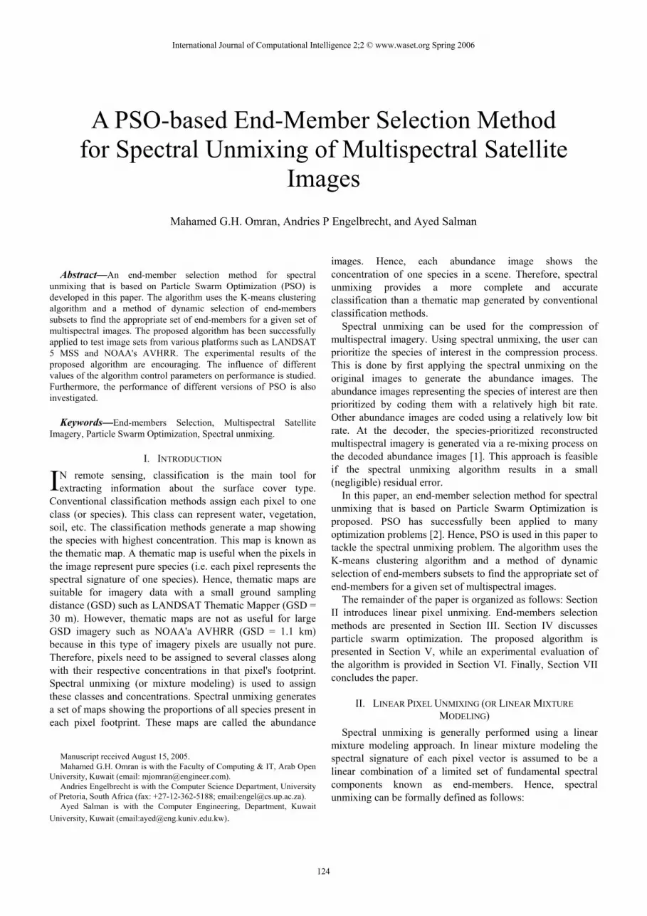
Fig. 1 Band 4 of the Landsat MSS test image of Lake Tahoe NOAA's AVHRR: Fig. 2 shows the five-channel

multispectral test image set of an almost cloud-free territory of the entire United Kingdom (UK). This image set was obtained from the University of Dundee Satellite Receiving Station. Each channel (one visible, one near-infra red and three in the thermal range) is comprised of a 847 × 1009, 10-bit per pixel (1024 gray levels) image and corresponds to a GSD of 1.1 km. The result of a preliminary principal component study of this

data set indicates that its intrinsic true spectral dimension eN is 3. As in [9], a total of eight end-members were obtained

from the data set (i.e. 8=mN ). The rest of this section is organized as follows: Section

VI.A illustrates that the PSO-EMS can be used successfully as

an end-member selection method by comparing it to the end-member selection method proposed by Saghri et al. [9] (i.e. ISO-UNMIX). Saghri et al. [9] showed that ISO-UNMIX performed very well compared to other popular spectral unmixing methods. Section VI.B investigates the influence of the different PSO-EMS control parameters. Finally, the uses of different PSO models (namely, gbest, lbest and lbest-to-gbest) are investigated in Section VI.C.

The results reported in this section are averages and standard deviations over 10 simulations. In addition, we start with an lbest implementation of the PSO (with zero-radius neighborhood) and linearly increase the neighborhood radius until a gbest implementation of the PSO is reached. In this paper, this approach is referred to as lbest-to-gbest-PSO. This hybrid approach is used in order to initially avoid being trapped in local optima, by initially using an lbest approach [23]. The algorithm then attempts to converge to the best solution found by the initial phase by using a gbest approach. The PSO-EMS parameters were initially set as follows: pkmeans = 0.1, s = 20, tmax = 100, number of K-means iterations is 10 (the effect of these values are then investigated), w =0.72,

1c = 2c = 1.49 and Vmax= 255 for the Lake Tahoe image set and Vmax = 1023 for the UK image set. No attempt was made

to tune the PSO parameters (i.e. w, 1c and 2c ) to each data set. The rationale behind this decision is the fact that in real-world applications the evaluation time is significant and as such parameter tuning is usually a time consuming process. These parameters are used in this section unless otherwise specified.

A. PSO-EMS vs. ISO_UNMIX This section presents results to compare the performance of

the PSO-EMS algorithm with that of the ISO-UNMIX algorithm for each of the test image sets.

Table I summarizes the results for the two image sets. The results are compared based on the RMS residual error (defined in (9)). The results showed that, for both image sets, PSO-EMS performed better than the ISO-UNMIX in terms of the RMS residual error. Figs. 3 and 4 show the abundance images generated from ISO-UNMIX and PSO-EMS, respectively, when applied to the Lake Tahoe image set. In addition, Figs. 5 and 6 show the abundance images generated from ISO-UNMIX and PSO-EMS, respectively, when applied to the UK image set. For display purposes the fractional species concentrations were mapped to 8 bits per pixels abundance images.


128

(a) Band 1 (b) Band 2

(c) Band 3 (d) Band 4

(e) Band 5 Fig. 2 AVHRR Image of UK, Size: 847x1009 , 5 bands, 10

bpp

TABLE I COMPARISON BETWEEN ISO-UNMIX AND PSO-EMS

Image RMS

LANDSAT 5 MSS ISO_UNMIX 0.491837

PSO-EMS 0.462197 ± 0.012074

NOAA's AVHRR ISO_UNMIX 3.725979

PSO-EMS 3.510287 ± 0.045442

B. Influence of PSO-EMS Parameters The PSO-EMS algorithm has a number of parameters that

have an influence on the performance of the algorithm. These parameters include Vmax, the swarm size, the number of PSO iterations, pkmeans and the number of K-means iterations. This section investigates the influence of different values of these parameters using the Lake Tahoe image set.

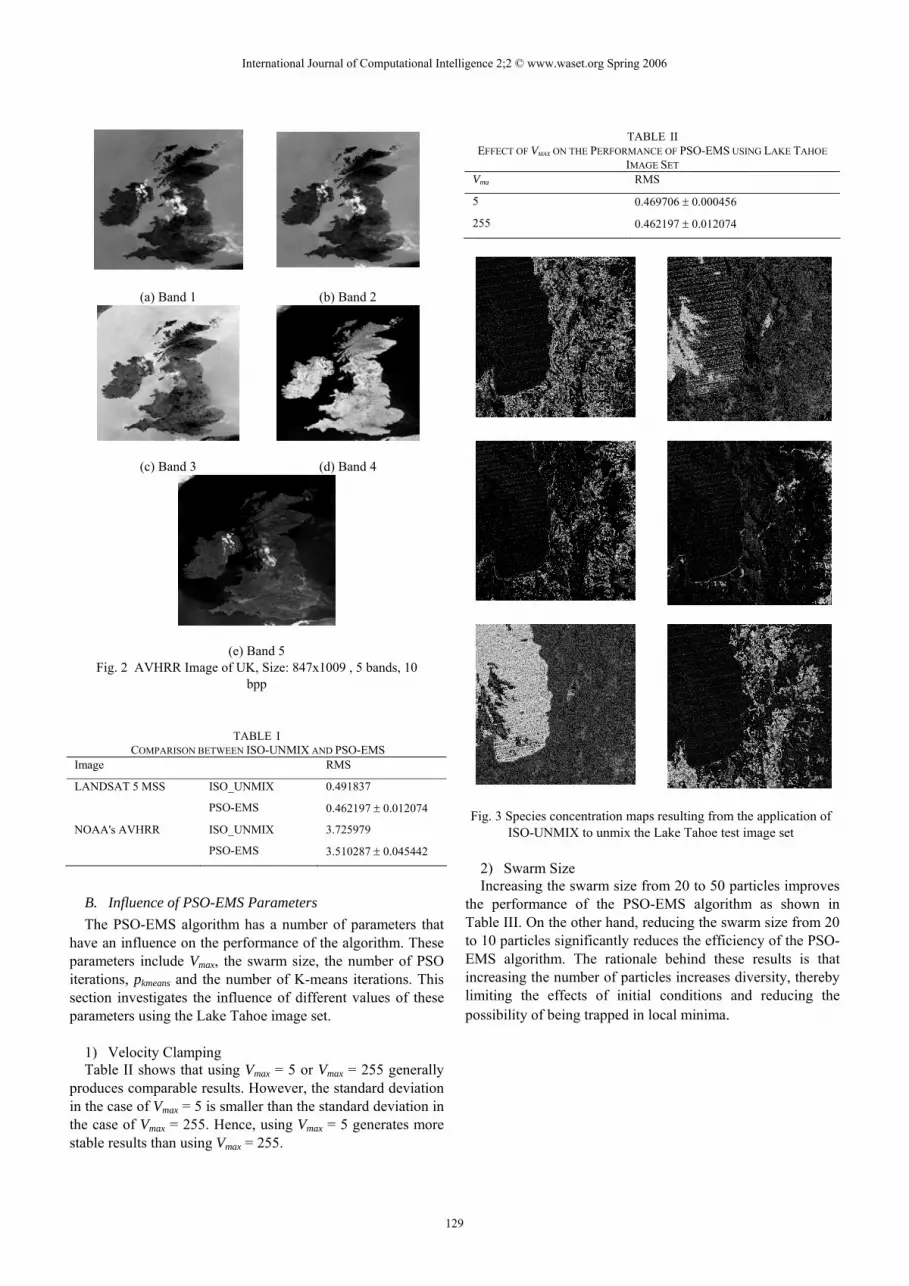
1) Velocity Clamping Table II shows that using Vmax = 5 or Vmax = 255 generally

produces comparable results. However, the standard deviation in the case of Vmax = 5 is smaller than the standard deviation in the case of Vmax = 255. Hence, using Vmax = 5 generates more stable results than using Vmax = 255.

TABLE II EFFECT OF VMAX ON THE PERFORMANCE OF PSO-EMS USING LAKE TAHOE

IMAGE SET Vma RMS

5 0.469706 ± 0.000456

255 0.462197 ± 0.012074

Fig. 3 Species concentration maps resulting from the application of ISO-UNMIX to unmix the Lake Tahoe test image set

2) Swarm Size Increasing the swarm size from 20 to 50 particles improves

the performance of the PSO-EMS algorithm as shown in Table III. On the other hand, reducing the swarm size from 20 to 10 particles significantly reduces the efficiency of the PSO-EMS algorithm. The rationale behind these results is that increasing the number of particles increases diversity, thereby limiting the effects of initial conditions and reducing the possibility of being trapped in local minima.


129

Fig. 4 Species concentration maps resulting from the application of PSO-EMS to unmix the Lake Tahoe test image set

TABLE III

EFFECT OF THE SWARM SIZE ON THE PERFORMANCE OF PSO-EMS USING LAKE TAHOE IMAGE SET

s RMS

10 0.468706 ± 0.004753

20 0.462197 ± 0.012074

50 0.459195 ± 0.009389

3) Number of PSO Iterations Reducing the number of PSO iterations, tmax, from 100 to 50

did not reduce the performance of the PSO-EMS algorithm as shown in Table IV. Similarly, increasing tmax from 100 to 150, did not significantly improve the performance of the PSO-EMS.

TABLE IV

EFFECT OF THE NUMBER OF PSO ITERATIONS ON THE PERFORMANCE OF PSO-EMS USING LAKE TAHOE IMAGE SET

tmax RMS

50 0.468041 ± 0.004735

100 0.462197 ± 0.012074

150 0.465614 ± 0.00739

Fig. 5 Species concentration maps resulting from the application of ISO-UNMIX to unmix the UK test image set

4) pkmeans Applying the K-means clustering algorithm to a larger set

of particles is expected to improve the performance of the PSO-EMS algorithm. The rationale behind this expectation is the fact that the K-means algorithm generally reduces the search space and refines the end-members. This expectation is verified by the results shown in Table V which shows that increasing the value of pkmeans significantly improves the performance of the PSO-EMS algorithm. However, as a trade-off, increasing the value of pkmeans will increase the computational requirements of the PSO-EMS algorithm.


130

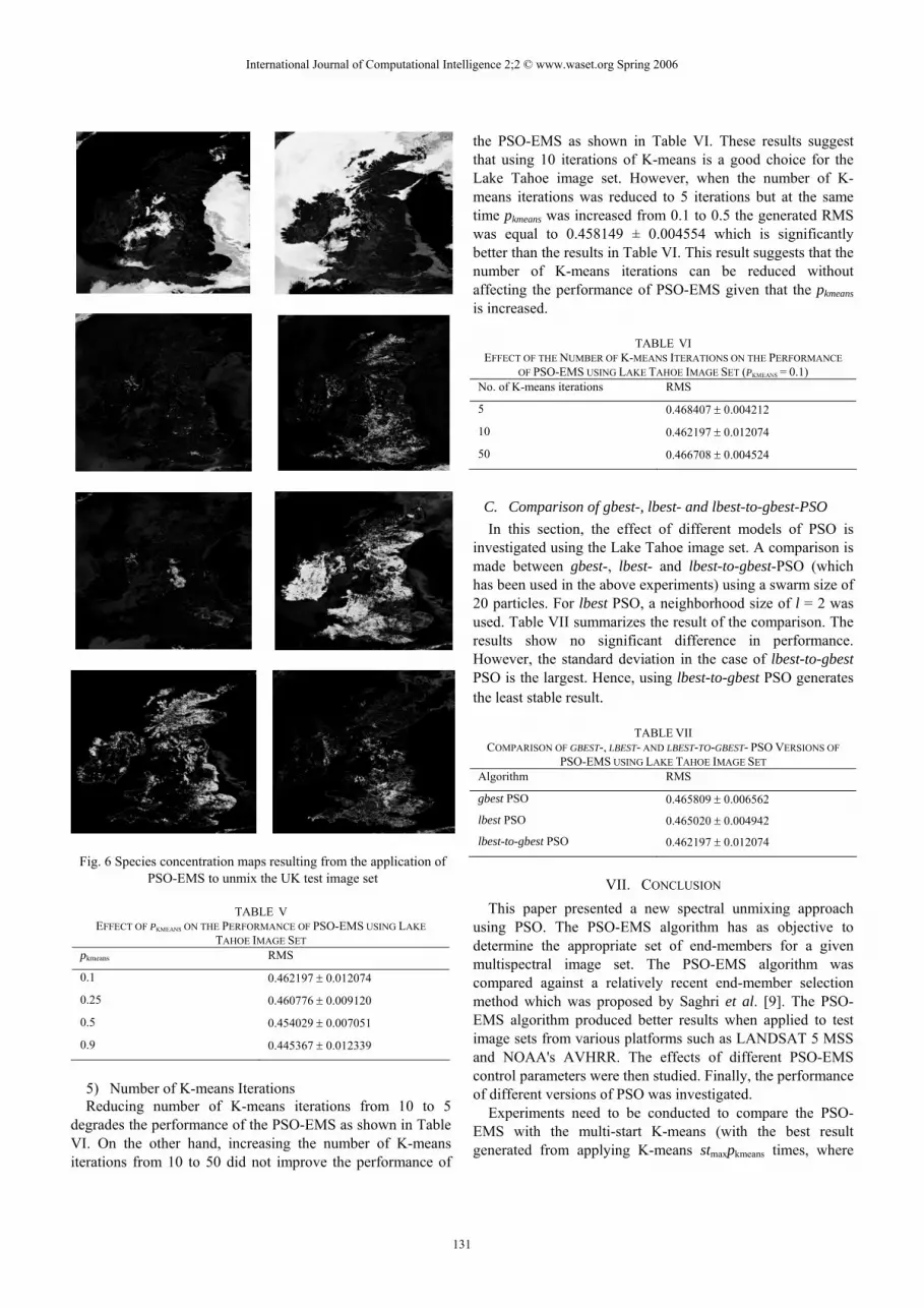
Fig. 6 Species concentration maps resulting from the application of PSO-EMS to unmix the UK test image set

TABLE V

EFFECT OF PKMEANS ON THE PERFORMANCE OF PSO-EMS USING LAKE TAHOE IMAGE SET

pkmeans RMS

0.1 0.462197 ± 0.012074

0.25 0.460776 ± 0.009120

0.5 0.454029 ± 0.007051

0.9 0.445367 ± 0.012339

5) Number of K-means Iterations Reducing number of K-means iterations from 10 to 5

degrades the performance of the PSO-EMS as shown in Table VI. On the other hand, increasing the number of K-means iterations from 10 to 50 did not improve the performance of

the PSO-EMS as shown in Table VI. These results suggest that using 10 iterations of K-means is a good choice for the Lake Tahoe image set. However, when the number of K-means iterations was reduced to 5 iterations but at the same time pkmeans was increased from 0.1 to 0.5 the generated RMS was equal to 0.458149 ± 0.004554 which is significantly better than the results in Table VI. This result suggests that the number of K-means iterations can be reduced without affecting the performance of PSO-EMS given that the pkmeans is increased.

TABLE VI EFFECT OF THE NUMBER OF K-MEANS ITERATIONS ON THE PERFORMANCE

OF PSO-EMS USING LAKE TAHOE IMAGE SET (PKMEANS = 0.1) No. of K-means iterations RMS

5 0.468407 ± 0.004212

10 0.462197 ± 0.012074

50 0.466708 ± 0.004524

C. Comparison of gbest-, lbest- and lbest-to-gbest-PSO In this section, the effect of different models of PSO is

investigated using the Lake Tahoe image set. A comparison is made between gbest-, lbest- and lbest-to-gbest-PSO (which has been used in the above experiments) using a swarm size of 20 particles. For lbest PSO, a neighborhood size of l = 2 was used. Table VII summarizes the result of the comparison. The results show no significant difference in performance. However, the standard deviation in the case of lbest-to-gbest PSO is the largest. Hence, using lbest-to-gbest PSO generates the least stable result.

TABLE VII COMPARISON OF GBEST-, LBEST- AND LBEST-TO-GBEST- PSO VERSIONS OF

PSO-EMS USING LAKE TAHOE IMAGE SET Algorithm RMS

gbest PSO 0.465809 ± 0.006562

lbest PSO 0.465020 ± 0.004942

lbest-to-gbest PSO 0.462197 ± 0.012074

VII. CONCLUSION This paper presented a new spectral unmixing approach

using PSO. The PSO-EMS algorithm has as objective to determine the appropriate set of end-members for a given multispectral image set. The PSO-EMS algorithm was compared against a relatively recent end-member selection method which was proposed by Saghri et al. [9]. The PSO-EMS algorithm produced better results when applied to test image sets from various platforms such as LANDSAT 5 MSS and NOAA's AVHRR. The effects of different PSO-EMS control parameters were then studied. Finally, the performance of different versions of PSO was investigated.

Experiments need to be conducted to compare the PSO-EMS with the multi-start K-means (with the best result generated from applying K-means stmaxpkmeans times, where


131

each K-means starts from random cluster centroids) and other spectral unmixing techniques on various AVHRR images. The performance of the PSO-EMS when applied to hyperspectral Satellite imagery is a potential topic for future research.

REFERENCES [1] J. Saghri, A. Tescher, M. Omran, Class-Prioritized Compression of

Multispectral Imagery Data, Journal of Electronic Imaging, vol. 11 (2), 246-256, 2002.

[2] J. Kennedy, R. Eberhart, Swarm Intelligence, Morgan Kaufmann, 2001. [3] J. J. Settle, N. A. Drake, Linear Mixing and Estimation of Ground Cover

Proportions, International Journal in Remote Sensing, vol. 14 (6), 1159-1177, 1993.

[4] J. Antoniades, D. Haas, P. Palmadesso, M. Baumback, L. J. Rickard, Use of Filter Vectors in Hyperspectral Data Analysis, In Proceedings of SPIE, vol. 2553, 128-139, 1995.

[5] A. Hlavka, M. A. Spanner, Unmixing AVHRR Imagery to Access Clearcuts and Forest Regrowth on Oregon, IEEE Transactions on Geoscience and Remote Sensing, vol. 33, 788-795, 1995.

[6] A. Bateson, B. Curtiss, A Method for Manual Endmember Selection and Spectral Unmixing, Remote Sensing of Enviornment, vol. 55, 229-243, 1996.

[7] F. Maselli, Multiclass Spectral Decomposition of Remotely Sensed Scenes by Selective Pixel Unmixing, IEEE Transactions on Geoscience and Remote Sensing, vol. 36 (5), 1809-1819, 1998.

[8] L. Parra, C. Spence, P. Sajda, A. Ziehe, K. Müller, Unmixing Hyperspectral Data, In Advances in Neural Information Processing Systems 12, MIT Press, 942-948, 2000.

[9] J. Saghri, A. Tescher, F. Jaradi, M. Omran, A Viable End-Member Selection Scheme for Spectral Unmixing of Multispectral Satellite Imagery Data, Journal of Imaging Science and Technology, vol. 44 (3), 196-203, 2000.

[10] A. Plaza, P. Martinez, R. Perez, J. Plaza, A Quantitative and Comparative Analysis of Endmember Extraction Algorithms from Hyperspectral Data, IEEE Transactions on Geoscience and Remote Sensing, vol. 42(3), 650-663, 2004.

[11] J. Crespo, R. Duro, F. Lopez-Pena, Spectral Unmixing Through Gaussian Synapse ANNs in Hyperspecteal Images, Proceedings of the 8th International Conference on Knowledge-Based Intelligent Information and Engineering Systems, Wellington, New Zealand, 661-668, 2004.

[12] M. Grana, A. D'Anjou, Feature Extraction by Linear Spectral Unmixing, Proceedings of the 8th International Conference on Knowledge-Based Intelligent Information and Engineering Systems, Wellington, New Zealand, 692-698, 2004.

[13] J. Zhang, B. Rivard, A. Sanchez-Azofeifa, Derivative Spectral Unmixing of Hyperspectral Data Applied to Mixtures of Lichen and Rock, IEEE Transactions on Geoscience and Remote Sensing, vol. 42(9), 1934-1940, 2004.

[14] S. McDonald, K. Niemann, D. Goodenough, Development of Hyperspectral Biochemistry through the use of Statistical Modeling and Spectral Unmixing, Proceedings of the IEEE International Geoscince and Remote Sensing Symposium, vol. 2, 1007-1009, 2004.

[15] M. Cauguy, M. Roggemann, T. Schulz, Spectral Unmixing Methods to Estimate Materials on Satellite Surface, Proceedings of the 36th Southeastern Symposium on System Theory, 11-15, 2004.

[16] J. Settle, On the Residual Term in Linear Mixture Model and its Dependence on the Point Spread Function, IEEE Transactions on Geoscience and Remote Sensing, vol. 43(2), 398-401, 2005.

[17] J. Broadwater, R. Meth and R. Chellappa, A hybrid Algorithm for Subpixel Detection in Hyperspectral Imagery, Proceedings of the IEEE International Geoscince and Remote Sensing Symposium, vol. 3, 1601-1604, 2004.

[18] C. Shah, P. Varshney, A Higher Order Statistical Appraoch to Spectral Unmixing of Remote Sensing Imagery, Proceedings of the IEEE International Geoscince and Remote Sensing Symposium, vol. 2, 1065-1068, 2004.

[19] G. Ball and D. Hall, A Clustering Technique for Summarizing Multivariate Data, Behavioral Science, vol. 12, 153-155, 1967.

[20] J. Kennedy, R. Eberhart, Particle Swarm Optimization, Proceedings of IEEE International Conference on Neural Networks, Perth, Australia, vol. 4, 1942-1948, 1995.

[21] A. Engelbrecht, Computational Intelligence: An Introduction, John Wiley and Sons, 2002.

[22] Y. Shi, R. Eberhart, Parameter Selection in Particle Swarm Optimization, Evolutionary Programming VII: Proceedings of EP 98, 591-600, 1998.

[23] P. Suganthan, Particle Swarm Optimizer with Neighborhood Optimizer, Proceedings of the Congress on Evolutionary Computation, 1958-1962, 1999.

[24] Y. Shi, R. Eberhart, A Modified Particle Swarm Optimizer, Proceedings of the IEEE International Conference on Evolutionary Computation, Piscataway, NJ, 69-73, 1998.

[25] J. Kennedy, Small Worlds and Mega-Minds: Effects of Neighborhood Topology on Particle Swarm Performance, Proceedings of the Congress on Evolutionary Computation, 1931-1938, 1999.

[26] J. Kennedy, R. Mendes, Population Structure and Particle Performance, Proceedings of the IEEE Congress on Evolutionary Computation, Honolulu, Hawaii, 2002.

[27] F. Van den Bergh, An Analysis of Particle Swarm Optimizers, PhD Thesis, Department of Computer Science, University of Pretoria, 2002.

[28] F. van den Bergh, A.P. Engelbrecht, A New Locally Convergent Particle Swarm Optimizer, Proceedings of the IEEE Conference on Systems, Man, and Cybernetics, Hammamet, Tunisia, 2002.

Mahamed G. H. Omran received his B.Sc. and M.Sc. degrees with Honors in Computer Engineering from Kuwait University, State of Kuwait, in 1998 and 2000, respectively. He completed his Ph.D. in the Department of Computer Science at University of Pretoria, South Africa, in April 2005. He is a member of the Computational Intelligence Research Group (http://cirg.cs.up.ac.za/) of the Department of Computer Science at University of Pretoria, South Africa.

His current research interest is in the area of computational intelligence with special emphasis on Particle Swarm Optimization (PSO) and Differential Evolution (DE). In addition, Dr. Omran is interested in the area of data clustering, unsupervised image classification and color image quantization. Andries Engelbrecht received the M.Sc and PhD degrees from the University of Stellenbosch, Stellenbosch, South Africa, in 1994 and 1999, respectively. He is a Full Professor at the Department of Computer Science, University of Pretoria, Pretoria, South Africa, leading a research group of three staff members and 45 Masters and PhD students.

His research interests include aspects of swarm intelligence, evolutionary computation, artificial immune systems, data mining, swarm robotics, and neural networks, with several publications in those fields. Prof. Engelbrecht is also a member of the IEEE CIS and its task forces on Evolutionary Computation and Games, Swarm Intelligence, and Coevolution. He is an associate editor of IEEE Transactions on Evolutionary Computation. He is the author of the book, "Computational Intelligence: An Introduction", Wiley, 2002, and recently authored the book "Computational Swarm Intelligence" to be published by Wiley. Ayed Salman received his MS and PhD degrees from Syracuse University, NY, USA, in 1996 and 1999, respectively. He is an Assistant Professor at the Department of Computer Engineering, Kuwait University, Kuwait.

His research interests include Application of evolutionary computations in data mining, web mining and multi-objective optimization; E-Commerce. Neural Network, Machine Learning.


132

Documents

A PSO-based end-member selection method for spectral unmixing of multispectral satellite images