Computers & Industrial Engineering 56 (2009) 87–96

Contents lists available at ScienceDirect

Computers & Industrial Engineering

journal homepage: www.elsevier .com/ locate/caie

A production–inventory model with remanufacturing for defective and usableitems in fuzzy-environment

Arindam Roy a,*, Kalipada Maity b, Samarjit kar c, Manoranjan Maiti d

a Department of Engineering Science, Haldia Institute of Technology, Haldia, Purba-Medinipur, W.B. 721657, Indiab Department of Mathematics, Mugberia Gangadhar Mahavidyalaya, Mugberia, Purba-Medinipur, W.B., Indiac Department of Mathematics, National Institute of Technology, Durgapur, W.B. 713209, Indiad Department of Mathematics and Computer Application, Guru Nanak Institute of Technology, Kolkata, W.B. 700114, India

a r t i c l e i n f o

Article history:Received 5 December 2007Received in revised form 7 April 2008Accepted 8 April 2008Available online 2 June 2008

Keywords:Finite time horizonRemanufacturingGenetic algorithmFuzzy defective rateCredibility

0360-8352/$ - see front matter � 2008 Elsevier Ltd. Adoi:10.1016/j.cie.2008.04.004

* Corresponding author.E-mail address: royarindamroy@yahoo.com (A. Ro

a b s t r a c t

This paper investigates a production–remanufacturing system for a single product over a known-finitetime horizon. Here the production system produces some defective units which are continuously trans-ferred to the remanufacturing unit and the constant demand is satisfied by the perfect items from pro-duction and remanufactured units. Remanufacturing unit uses the defective items from productionunit and the collected used-products from the customers and later items are remanufactured for reuseas fresh items. Some of the used items in the remanufacturing unit are disposed off which are not repair-able. The remanufactured units are treated as perfect items. Normally, rate of defectiveness varies in aproduction system and may be approximated by a constant or fuzzy parameter. Hence, two modelsare formulated separately with constant and fuzzy defective productions. When defective rate is impre-cise, optimistic and pessimistic equivalent of fuzzy objective function is obtained by using credibilitymeasure of fuzzy event by taking fuzzy expectation. Here, it is assumed that remanufacturing systemstarts from the second production cycle and after that both production and remanufacturing units con-tinue simultaneously. The models are formulated for maximum total profit out of the whole system. Herethe decision variables are the total number of cycles in the time horizon, the duration for which the defec-tive items are collected and the cycle length after the first cycle. Genetic Algorithm is developed withRoulette wheel selection, Arithmetic crossover, Random mutation and applied to evaluate the maximumtotal profit and the corresponding optimum decision variables. The models are illustrated with somenumerical data. Results of some particular cases are also presented.

� 2008 Elsevier Ltd. All rights reserved.

1. Introduction

Till now, the resource and other constraints used in a decisionmaking problem are normally considered to be either determinis-tic or stochastic only. But, in real-life situation these constraintsmay be of imprecise type, i.e., uncertainty is to be imposed innon-stochastic sense. Zadeh (1978) and Dubois and Prade (1988)introduced the necessity and possibility constraints which are veryrelevant to the real-life decision making problems and presentedthe process of defuzzification for these constraints. Later, Liu andIwamura (1998) extended these ideas and applied in linear/nonlin-ear programming problems.

During the last two decades many researchers (cf. Maity & Maiti(2005), Sana, Goyal, & Chaudhuri (2004), Cho (1996)) have givenconsiderable attention to the area of production inventory prob-lem. But classical logistic systems manage the material and relatedinformation flow until the final products are delivered to the cus-

ll rights reserved.

y).

tomer. This means a forward flow, reverse logistic manages back-ward process, i.e., the used and reusable parts are returned fromthe customers to the producer. Environmental consciousnessforces companies to initiate such product recovery systems withtheir disposal (metal, glass, paper). Recent reviews on reverselogistics are provided by Fleischmann et al. (1997), Guide, Jayar-aman, Srivastava, and Benton (1998) and Gupta and Gungor(1999), Koh, Hwang, Sohn, and Ko (2002), Dobos (2003), Wee,Yu, Lo, and Chen (2005), Wee, Yu, Su, and Wu (2006b) and others.

Since remanufactured products are as-good-as-new, these canbe used to satisfy the demands for new product. Hence, at leastsome demands are satisfied by remanufacturing (new) products.Such situations with both manufacturing and remanufacturinglead to interesting questions from an inventory control point ofview. For what duration should the products be manufactured orremanufactured? When should returned products be disposed ofor collection of returned products be discontinued? What shouldbe the amount of inventory quantities?

In recent years, many researchers have studied these questions.Some obtained structural results about the form of the optimal

88 A. Roy et al. / Computers & Industrial Engineering 56 (2009) 87–96

inventory control policy. Others found (nearly) optimal policieswithin some prespecified class. For a review, we refer to Fleisch-mann et al. (1997).

In most of the classical economic production quantity (EPQ)model, it is assumed that items produced are of perfect quality,though the quality control of the product generally is not consid-ered. However, in a production system, it is quite natural that amachine can not produce all items perfect during whole produc-tion period. Hayek and Salameh (2001) derived an optimal operat-ing policy for the finite production model under the effect ofreworking of imperfect items assuming that all the defective itemsare repairable. Chiu (2003) examined an EPQ model with scrapitems and the reworking of repairable items. Recently,Wee, Yu,and Chen (2007) developed an optimal inventory model for itemswith imperfect quality and backlogged shortage.

Richter (1996a, 1996b, 1997), Richter and Dobos (1999) haveinvestigated a waste disposal model, where the return rate is adecision variable. They have given the optimal number of manu-facturing and production batches depending on the return rate.Richter (1997) in his paper has examined the optimal inventoryholding policy, if the waste disposal (return)rate is a decision var-iable. Dobos and Richter (2004, 2006) have investigated a produc-tion/recycling model with stationary demand and return rates andquality consideration, respectively. Chung, Wee, and Yang (inpress) and Wee and Chung (2008) have developed inventory mod-els with remanufacturing. Recently, there are some inventory con-trol problems which have been formulated in fuzzy environment.Wee, Lo, and Hsu (accepted) developed an inventory model fordeteriorating items in a fuzzy environment. Dey, Kar, and Maiti(2005) developed an inventory model in fuzzy environment usingnearest interval approximation. Wang and Shu (2005) developed asupply chain inventory model under possibility constraints. Maitiand Maiti (2006) solved a fuzzy inventory model with two ware-houses under necessity constraints. Using the possibility andnecessity idea we introduce here a credibility measure to findout the crisp value of a fuzzy variable which is also called expectedvalue of a fuzzy variable (cf. Liu & Liu (2002)). Till now, none hasformulated production-remanufacturing inventory system in fuzzyenvironment. The motive of the present paper is to illustrate theformulation of a realistic production inventory model for a reus-able and defective item with remanufacturing and fuzzy defectiverate and to derive equivalent crisp value of a fuzzy expressionusing credibility measure. Here, realistically, it is assumed thatuse of remanufacturing system linearly depends on the volumeof market demand and the production of the remanufacturing sys-tem. So far, none considered these factors.

Hence, for the first time, a system with production and reman-ufacturing units working simultaneously has been considered in afuzzy environment with imprecise defective produced units. Herewe introduce a rate of usable items collected from the market,which is more realistic and virgin. Possibility and necessity con-cepts have been introduced in such a model. Some realisticassumptions such as market demand being met from both freshand remanufactured units, remanufactured units being dependenton fresh units produced, etc., have not been considered, till now, byearlier workers where as these have been taken into account in thispaper.

In this paper, a production–recycling inventory system hasbeen developed under imprecise environment. By using expectedvalue of fuzzy variable (cf. Liu & Liu (2002)), the crisp value ofthat fuzzy variable is obtained and applied to a production–recy-cling inventory problem. Here, it is also assumed that there is nodifference between newly produced and recycled items. Inventoryholding cost parameter for manufactured items is higher thanthat for the remanufactured/recycled product. Here, remanufac-turing starts from the 2nd cycle. In the first cycle, production rate

is constant and in other cycles, production rate is dependent onremanufacturing rate and remanufacturing rate depends on mar-ket demand. The model has been formulated as a profit maximiz-ing problem and optimum results are obtained though a realcoded Genetic Algorithm developed for this purpose. Here, totalnumber of cycles in the finite horizon, the duration for whichthe defective units are collected and the cycle length after thefirst cycle are the decision variables. A numerical experiment isperformed to illustrate the model and results for several particu-lar cases are derived out of the general result. For the first time, asystem with production and remanufacturing units workingsimultaneously has been considered in fuzzy environment withimprecise defective produced units. Possibility and necessity con-cepts have introduced in such a model. Some realistic assump-tions such as market demand dependent remanufacturingproduction, remanufactured items dependent fresh units produc-tion, etc., not considered by earlier workers have been taken intoaccount. The whole paper has been organized as: in Section 2,assumptions and notations, in Section 3, model developmentand analysis, in Section 4, solution methodology (GA), are pre-sented. Numerical experiment is performed and results are pre-sented in Section 5. In Sections 6–8 some discussions, practicalimplication and conclusion are made. Expected value operatorand genetic algorithm (GA) are presented in Appendix A andAppendix B, respectively.

2. Assumptions and notations

The mathematical model in this paper is developed on the basisof following assumptions and notations:

(i) Inventory system involves only one item.(ii) The time horizon T is finite and known.

(iii) No shortages are permitted.(iv) Lead time is zero.(v) N is the total number of cycles in T and is a decision

variable.(vi) k is the number cycles up to which usable items are pur-

chased and is a decision variable.(vii) t1 is the time period in kth cycle up to which usable items

are collected for remanufacturing.(viii) Some defective units are produced during production

time at the rate of d ð0 < d < 1Þ, may be crisp or fuzzy.(ix) Total time horizon consists of N cycles where N is a deci-

sion variable.(x) P1, the production rate in first cycle is constant.

(xi) D is the demand rate (deterministic and known).(xii) Remanufacturing rate, P2 ¼ P02 þ k1D; P02; k1 > 0.

(xiii) Production rate in other cycles, P01 ¼ P001 þk2Pc

2; P001; k2 > 0.

(xiv) ciZ is the disposal rate in i-th cycle, whereci ¼ c1 þ ði� 1Þh1; c1 ¼ 1; h1 > 0; Z > 0;8i ¼ 1;2; . . . ; k.

(xv) tr = time period of the first cycle.(xvi) t0r = time period of the other cycles, it is a decision

variable.(xvii) tp = production time period of the first cycle.

(xviii) t0p = production time period of the other cycles.(xix) aijD = rate of usable items collected from the market for j-

th cycle when total time horizon consists of i cycles.ðj ¼ 1;2; . . . ; iÞ and aij ¼ aiþ1;jþ1 < 18i; j.

aii ¼ a118i ¼ 1;2; . . . ;n.ai;j�1 ¼ aij þ h;ai;j�2 ¼ ai;j�1 þ h ¼ aij þ 2h and so on.Also,

Pir¼1air ¼ i:a11 þ iði�1Þ

2 h;h > 0.(xx) xsðtÞ = on-hand inventory of the serviceable item at time t.

(xxi) xnsðtÞ = on-hand inventory of the non-serviceable item attime t.

A. Roy et al. / Computers & Industrial Engineering 56 (2009) 87–96 89

(xxii) s = selling price per unit.(xxiii) tr = time period of the first cycle.(xxiv) C1 = holding cost of serviceable item per unit per unit

time.(xxv) C2 = holding cost of non-serviceable item per unit per unit

time.(xxvi) Cp = production cost per unit.

(xxvii) CR = remanufacturing cost per unit.(xxviii) Cd = purchasing cost of usable items per unit from the

market.(xxix) C3 = ordering/set-up cost per cycle.(xxx) TP = total profit.

3. Model development and analysis

In this proposed model, we have considered an imperfect man-ufacturing system with remanufacturing of defective units. For thedevelopment of this model, we assume that there are N productioncycles during the finite time horizon T. Remanufacturing startsfrom second cycle and continues up to last cycle. During first cycledemand is satisfied by good units from the production only and forother cycles demand is met from production and remanufacturingboth. Here, non-serviceable items which are used-items collectedfrom the market and defective productions are remanufactured.Before remanufacturing, some collected non-serviceable itemswhich are not in a position for remanufacturing are disposed.

Let the material flow of production–recycling model, P1 is theconstant production rate in first cycle. P01 is the production ratein other cycles which depends on remanufacturing rate, xsðtÞ isthe on-hand inventory of the serviceable item at time t. Here

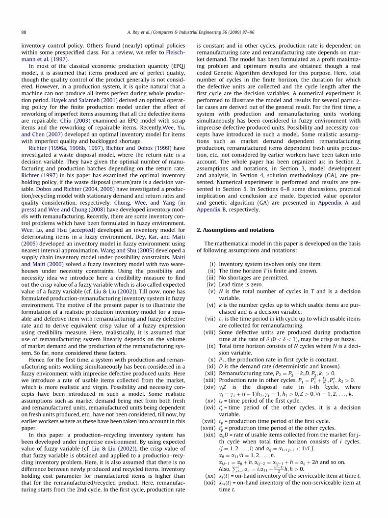
Fig. 1. Membership function of TFN ~a.

Fig. 2. The material flow of pro

non-serviceable items xnsðtÞ, which are used items collectedat the rate

Pir¼1air

� �D

n ofrom the market and defective produc-

tions {at the rate dP1 and dP01} are remanufactured. Before reman-ufacturing some collected non-serviceable items which are not in aposition for remanufacturing are disposed off at the rate of iZ. Thisconfiguration is presented in Fig. 2.

3.1. Formulation for first cycle

The differential equation describing the serviceable inventorylevel xsðtÞ in the interval 0 < t < tr is given by,

dxsðtÞdt

¼ ð1� dÞP1 � D; 0 6 t 6 tp; ð1Þ

dxsðtÞdt

¼ �D; tp 6 t 6 tr; ð2Þ

where d > 0 with boundary conditions xsðtÞ ¼ 0 at t ¼ 0 and t ¼ tr .The differential equation describing the non-serviceable inven-

tory level xnsðtÞ in the interval 0 < t < tr is given by,

dxnsðtÞdt

¼ a11Dþ dP1 � Z; ð0 < a11 < 1Þ; 0 6 t 6 tr ; ð3Þ

where a11; d > 0 with boundary condition xnsðtÞ ¼ 0 at t ¼ 0.The solutions of the differential Eqs. (11) and (12) are given by,

xsðtÞ ¼fð1� dÞP1 � Dgt; 0 6 t 6 tp

Dðtr � tÞ; tp 6 t 6 tr:

�ð4Þ

The solutions of the differential Eq. (13) is given by,

xnsðtÞ ¼ ða11Dþ dP1 � ZÞt; 0 6 t 6 tr: ð5Þ

From (4) we get,

tp ¼Dtr

ð1� dÞP1: ð6Þ

In the first cycle, holding cost for the serviceable item is given by,

HCS1 ¼ C1

Z tp

0xsðtÞdt þ C1

Z tr

tp

xsðtÞdt

¼ C1fð1� dÞP1 � Dgt2

p

2þ C1D

ðtr � tpÞ2

2:

In the first cycle, holding cost for the non-serviceable item is givenby,

HCN1 ¼ C2

Z tr

0xnsðtÞdt ¼ C2ða11Dþ dP1 � ZÞ t

2r

2:

duction–recycling model.

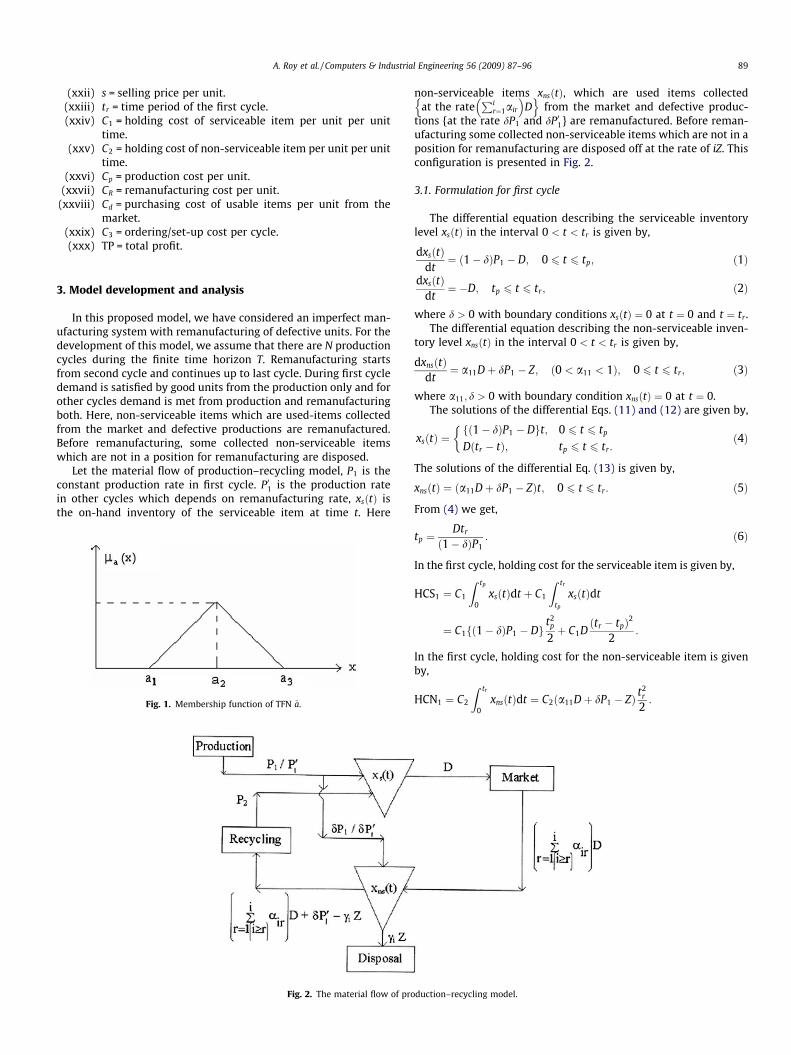
Fig. 3(a). Inventory level for serviceable item.

Fig. 3(b). Inventory level for non-serviceable item.

90 A. Roy et al. / Computers & Industrial Engineering 56 (2009) 87–96

Selling price in first cycle ¼ sDtr .Production cost in first cycle ¼ CpP1tp.Purchasing cost for used items in first cycle ¼ Cda11Dtr .Set-up cost ¼ C3.So, total profit in first cycle is given by (see Figs. 3a and b),

Tp1 ¼ sDtr � C1fð1� dÞP1 � Dgt2

p

2� C1:D

ðtr � tpÞ2

2

� C2ða11Dþ dP1 � ZÞ t2r

2� CpP1tp � Cda11Dtr � C3: ð7Þ

3.2. Formulation for ith ð2 6 i 6 NÞ cycle

The differential equation describing the serviceable inventory le-vel xsðtÞ in the interval ðtr þ ði� 2Þt0r 6 t 6 tr þ ði� 1Þt0rÞ is given by,

dxsðtÞdt

¼ ð1� dÞP01 þ P2 � D; tr þ ði� 2Þt0r 6 t 6 tr þ ði� 2Þt0r þ t0p;

ð8ÞdxsðtÞ

dt¼ P2 � D; tr þ ði� 2Þt0r þ t0p 6 t 6 tr þ ði� 1Þt0r; ð9Þ

where P2 < D with boundary conditions xsðtÞ ¼ 0 at t ¼ trþði� 2Þt0r and t ¼ tr þ ði� 1Þt0r .

The differential equation describing the non-serviceable inven-tory level xnsðtÞ in the interval ðtr þ ði� 2Þt0r 6 t 6 tr þ ði� 1Þt0rÞ isgiven by,

dxnsðtÞdt

¼Xi

r¼1

airDþ dP01 � P2 � ciZ; tr þ ði� 2Þt0r 6 t 6 tr

þ ði� 1Þt0r; i P r; i ¼ 2;3; . . . k� 1; ð10Þ

dxnsðtÞdt

¼Xk

r¼1

airDþ dP01 � P2 � ckZ; tr þ ðk� 2Þt0r 6 t 6 tr

þ ðk� 2Þt0r þ t1; ð11ÞdxnsðtÞ

dt¼ dP01 � P2; tr þ ðk� 2Þt0r þ t1 6 t 6 tr þ ðN � 1Þt0r; ð12Þ

wherePi

r¼1air ¼ ia11 þ iði�1Þ2 h 6 1;8i ¼ 2;3; . . . . . . ; k, with boundary

conditions xnsðtÞ ¼ 0 at t ¼ tr þ ðN � 1Þt0r .Using solutions of (11) and (12) we get,

t1 ¼1

ka11 þ kðk�1Þ2 h

n oD� ckZ

h i ðP2 � dP01Þ:ðN � kÞ:t0r�

�ða11:Dþ d:P1 � ZÞ:tr �Xk�2

p¼2

pa11 þpðp� 1Þ

2h

� �Dt0r

þðk� 3ÞðP2 � dP01Þt0r þXk�2

p¼2

cp:Z:t0r

� ðk� 1Þa11 þðk� 1Þðk� 2Þ

2h

� �D� ck�1Z � ðP2 � dP01Þ

� �:t0r

:

ð13Þ

A. Roy et al. / Computers & Industrial Engineering 56 (2009) 87–96 91

The solutions of the differential Eqs. (8) and (9) are given by,

xsðtÞ ¼

fð1� dÞP01 þ P2 � Dgft � ðtr þ ði� 2Þt0rÞg;tr þ ði� 2Þt0r 6 t 6 tr þ ði� 2Þt0r þ t0pðP2 � DÞft � ðtr þ ði� 1Þt0rÞg;

tr þ ði� 2Þt0r þ t0p 6 t 6 tr þ ði� 1Þt0r :

8>>>><>>>>: ð14Þ

From (14) we get,

t0p ¼ �ðP2 � DÞð1� dÞP01

t0r where t0r ¼ðT � trÞðN � 1Þ : ð15Þ

Holding cost for serviceable item is given by,

HCSi ¼ C1

Z trþði�2Þt0rþt0p

trþði�2Þt0rxsðtÞdt þ C1

Z trþði�1Þt0r

trþði�2Þt0rþt0p

xsðtÞdt

¼ C1fð1� dÞP01 þ P2 � Dg

2t20

p �ðP2 � DÞ

2ðt0p � t20

r Þ

: ð16Þ

Holding cost of non-serviceable item for 2nd cycle is given by,

HCN2 ¼ C2

Z trþt0r

tr

xnsðtÞdt

¼ C2

Z trþt0r

tr

fð2a11 þ hÞD� c2Z � ðP2 � dP01Þgðt � trÞ�

þða11Dþ dP1 � ZÞtr �dt ¼ C2

2fð2a11 þ hÞD� c2Z

�ðP2 � dP01Þgt20r þ C2:ða11Dþ dP1 � ZÞtr :t0r : ð17Þ

Holding cost of non-serviceable item for ithð3 6 i 6 k� 1Þ cycle isgiven by,

HCNi¼C2

Z trþði�1Þt0r

trþði�2Þt0rxnsðtÞdt¼C2

Z trþði�1Þt0r

trþði�2Þt0rða11DþdP1�ZÞtr½

þXi�1

p¼2

pa11þpðp�1Þ

2h

� �Dt0r�ði�2ÞðP2�dP01Þt0r

�Xi�1

p¼2

cp:Z:t0rþ ia11þ

iði�1Þ2

h� �

D�ciZ�ðP2�dP01Þ� �

:

� t�ðtrþði�2Þt0rÞ)#

dt¼C2: ða11DþdP1�ZÞtr :t0r�(

þXi�1

p¼2

pa11þpðp�1Þ

2h

� �Dt20

r �ði�2ÞðP2�dP01Þt20r

�Xi�1

p¼2

cp:Z:t02r þ ia11þ

iði�1Þ2

h� �

D�ciZ�ðP2�dP01Þ� �

:12:t20

r

#:

ð18ÞHolding cost of non-serviceable item for k-th cycle is given by,

HCNk ¼ C2

Z trþðk�2Þt0rþt1

trþðk�2Þt0rxnsðtÞdt þ C2

Z trþðk�1Þt0r

trþðk�2Þt0rþt1

xnsðtÞdt

¼ C2

Z trþðk�2Þt0rþt1

trþðk�2Þt0rða11Dþ dP1 � ZÞtr½

þXk�2

p¼2

pa11 þpðp� 1Þ

2h

� �Dt0r � ðk� 3ÞðP2 � dP01Þt0r

�Xk�2

p¼2

cp:Z:t0r þ ðk� 1Þa11 þ

ðk� 1Þðk� 2Þ2

h� �

D� ck�1Z�

�ðP2 � dP01Þ�:t0r þ ka11 þ

kðk� 1Þ2

h� �

D� ckZ�

�ðP2 � dP01Þ�: t � tr þ ðk� 2Þt0r

� � �dt

þC2

Z trþðk�1Þt0r

trþðk�2Þt0rþt1

ðP2 � dP01Þ:ðN � kÞt0r�

þðP2 � dP01Þftr þ ðk� 1Þt0rg � ðP2 � dP01Þt�dt

¼C2: ða11DþdP1�ZÞtr:t1þXk�2

p¼2

pa11þpðp�1Þ

2h

� �Dt0r :t1

"

�ðk�3ÞðP2�dP01Þt0r:t1�Xk�2

p¼2

cp:Z:t0r:t1

þ ðk�1Þa11þðk�1Þðk�2Þ

2h

� �D�ck�1Z�ðP2�dP01Þ

�:t0r :t1

�þ ka11þ

kðk�1Þ2

h� �

D�ckZ�ðP2�dP01Þ� �

t21

2

#þC2:ðP2�dP01Þ:ðN�kÞ:t0r:ðt0r� t1ÞþC2:ðP2�dP01Þ:ftrþðk�1Þt0rg:ðt0r� t1Þ

�C2

2ðP2�dP01Þ

�trþðk�1Þt0r� �2� trþðk�2Þt0rþ t1

� �2�:

ð19ÞHolding cost of non-serviceable item for ithððkþ 1Þ 6 i 6 nÞ cycle isgiven by,

HCNi ¼ C2

Z trþðN�1Þt0r

trþðk�1Þt0rxnsðtÞdt

¼ C2

Z trþðN�1Þt0r

trþðk�1Þt0rðdP01 � P2Þ: t � ðtr þ ðN � 1Þt0rÞ

�� �dt

¼ C2ðP2 � dP01Þ

2:ðN � kÞ2:t02r : ð20Þ

Total purchasing cost for used items is given by,

Ccost ¼ Cd

Xk�1

i¼2

ia11 þiði� 1Þ

2h

� �Dt0r þ ka11 þ

kðk� 1Þ2

h� �

D:t1

" #:

ð21ÞTotal production cost for ðN � 1Þ cycles is given by,

PC ¼ ðN � 1Þ:Cp:P01:t0p: ð22Þ

Total remanufacturing cost is given by,RC ¼ CR:P2:ðT � trÞ: ð23ÞTotal set-up cost for ðN � 1Þ cycles ¼ ðN � 1Þ:C3.

Sales revenue for ðN � 1Þ cycles ¼ s:D:ðT � trÞ.

3.3. Total profit of the system

Total holding cost for serviceable stock is given by,

HCS ¼ HCS1 þXN

i¼2

HCSi: ð24Þ

Total holding cost for non-serviceable stock is given by,

HCN ¼ HCN1 þXN

i¼2

HCNi: ð25Þ

Total profit is given by,

TPðN; k; t0rÞ ¼ hSalesrevenuei � hTotalproductioncosti� hTotalremanufacturingcosti � hTotalpurchasingcosti� hTotalholdingcosti � hTotalsetupcosti ¼ sDT � Cp:P1:tp

� ðN � 1Þ:Cp:P01:t0p � C1fð1� dÞP1 � Dg

t2p

2� C1D

ðtr � tpÞ2

2

� ðN � 1ÞC1fð1� dÞP01 þ P2 � Dg

2t02p �

ðP2 � DÞ2

ðt0p � t0rÞ2

� C2ða11Dþ dP1 � ZÞ t

2r

2� C2

2

nð2a11 þ hÞD� c2Z � ðP2 � dP01Þ

ot02r

� C2:ða11Dþ dP1 � ZÞtr :t0r � C2:Xk�1 h

ða11Dþ dP1 � ZÞtr :t0r

i¼3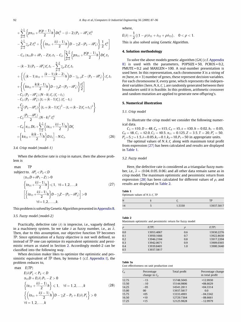

92 A. Roy et al. / Computers & Industrial Engineering 56 (2009) 87–96

þXi�1

p¼2

pa11 þpðp� 1Þ

2h�

Dt02r � ði� 2ÞðP2 � dP01Þt02r�

�Xi�1

p¼2

cp:Z:t02r þ ia11 þ

iði� 1Þ2

h� �

D� ciZ�ðP2 � dP01Þ):12:t02r

( #

� C2:ða11Dþ dP1 � ZÞtr:t1 � C2:Xk�2

p¼2

pa11 þpðp� 1Þ

2h

� �Dt0r :t1

"

� ðk� 3ÞðP2 � dP01Þt0r:t1 �Xk�2

p¼2

cp:Z:t0r:t1

þ ðk� 1Þa11 þðk� 1Þðk� 2Þ

2h

� �D� ck�1Z � ðP2 � dP01Þ

� �:t0r:t1

þ ka11þkðk�1Þ

2h

� �D�ckZ�ðP2�dP01Þ

)t2

1

2

( #�C2:ðP2�dP01Þ:ðN�kÞ:t0r:ðt0r� t1Þ�C2:ðP2�dP01Þ:ftrþðk�1Þt0rg:ðt0r� t1Þ

þC2

2ðP2�dP01Þ

(trþðk�1Þt0r� �2�ðtrþðk�2Þt0rþ t1Þ2

)

�C2ðP2�dP01Þ

2:ðN�kÞ2:t02r

�Cd

"a11:Dtrþ

Xk�1

i¼2

ia11þiði�1Þ

2h

� �Dt0r

þ ka11þkðk�1Þ

2h

� �D:t1

�N:C3: ð26Þ

Table 1Optimum values of N; k; t0r ;TP

N k t0r TP

14 5 1.5330 13937.5817

Table 2Maximum optimistic and pessimistic return for fuzzy model

q EðTPÞ q EðTPÞ

0.0 13953.4067 0.6 13930.22760.1 13950.1666 0.7 13922.86300.2 13946.2184 0.8 13917.22040.3 13942.0671 0.9 13909.03650.4 13939.8401 1.0 13900.36400.5 13937.5817

Table 3aCost effectiveness on unit production cost

Cp Percentagechange in Cp

Total profit Percentage changein total profit

12.75 �15 15748.5045 +12.993013.50 �10 15144.9806 +08.662914.25 �05 14541.2811 +04.331415.00 00 13937.5817 0.015.75 +05 13333.4901 �04.334216.50 +10 12729.7364 �08.666117.25 +15 12125.9828 �12.9979

3.4. Crisp model (model-1)

When the defective rate is crisp in nature, then the above prob-lem is

max TPsubject to; dP01<P2<D

ða11DþdP1�ZÞ>0

ia11þiði�1Þ

2h

� �61; 8i¼1;2; . . . ;k

ia11þiði�1Þ

2h

� �D�ciZ�ðP2�dP01Þ

>0

8i¼1;2; . . . ::;k:

ð27Þ

This problem is solved by Genetic Algorithm presented in Appendix B.

3.5. Fuzzy model (model-2)

Practically, defective rate ðdÞ is imprecise, i.e., vaguely definedin a machinery system. So we take d as fuzzy number, i.e., as ed.Then, due to this assumption, our objective function TP becomesfTP . Since optimization of a fuzzy objective is not well defined, soinstead of fTP one can optimize its equivalent optimistic and pessi-mistic return as stated in Section 2. Accordingly model-2 can beclassified into the following way.

When decision maker likes to optimize the optimistic and pes-simistic equivalent of fTP then, by lemma-1 (c.f. Appendix I), theproblem reduces to,

max EðTPÞEðdÞP01 < P2 < D

a11Dþ EðdÞ:P1 � Z > 0

ia11 þiði� 1Þ

2h

� �6 1; 8i ¼ 1;2; . . . ; k

ia11 þiði� 1Þ

2h

� �D� ciZ � P2 þ EðdÞ:P01

� �> 0

8i ¼ 1;2; . . . ; k

ð28Þ

where,

EðdÞ ¼ 12ð1� qÞd11 þ d12 þ qd13f g; 0 < q < 1:

This is also solved using Genetic Algorithm.

4. Solution methodology

To solve the above models genetic algorithm (GA) (c.f. AppendixII) is used with the parameters, POPSIZE = 50, PCROS = 0.2,PMUTE = 0.2 and MAXGEN = 100. A real-number presentation isused here. In this representation, each chromosome X is a string ofm (here, m = 3) number of genes, these represent decision variables.For each chromosome X, every gene, which represents the indepen-dent variables (here, N, k, t0r ), are randomly generated between theirboundaries until it is feasible. In this problem, arithmetic crossoverand random mutation are applied to generate new offspring’s.

5. Numerical illustration

5.1. Crisp model

To illustrate the crisp model we consider the following numer-ical data.

C3 ¼ $10;D ¼ 48;Cp ¼ $15;Cd ¼ $5; s ¼ $30;h ¼ 0:02;h1 ¼ 0:05;CR ¼ $8; C1 ¼ $2:0; C2 ¼ $0:5;a11 ¼ 0:125; Z ¼ 3:5; T ¼ 20; P001 ¼ 50;P02¼5;c¼1:5;d¼0:05;k1¼0:1;k2¼10;P1¼50 in appropriate units.

The optimal values of N; k; t0r along with maximum total profitfrom expression (27) has been calculated and results are displayedin Table 1.

5.2. Fuzzy model

Here, the defective rate is considered as a triangular fuzzy num-ber, i.e., ed ¼ ð0:04;0:05; 0:06Þ and all other data remain same as incrisp model. The maximum optimistic and pessimistic return fromexpression (28) has been calculated for different values of q, andresults are displayed in Table 2.

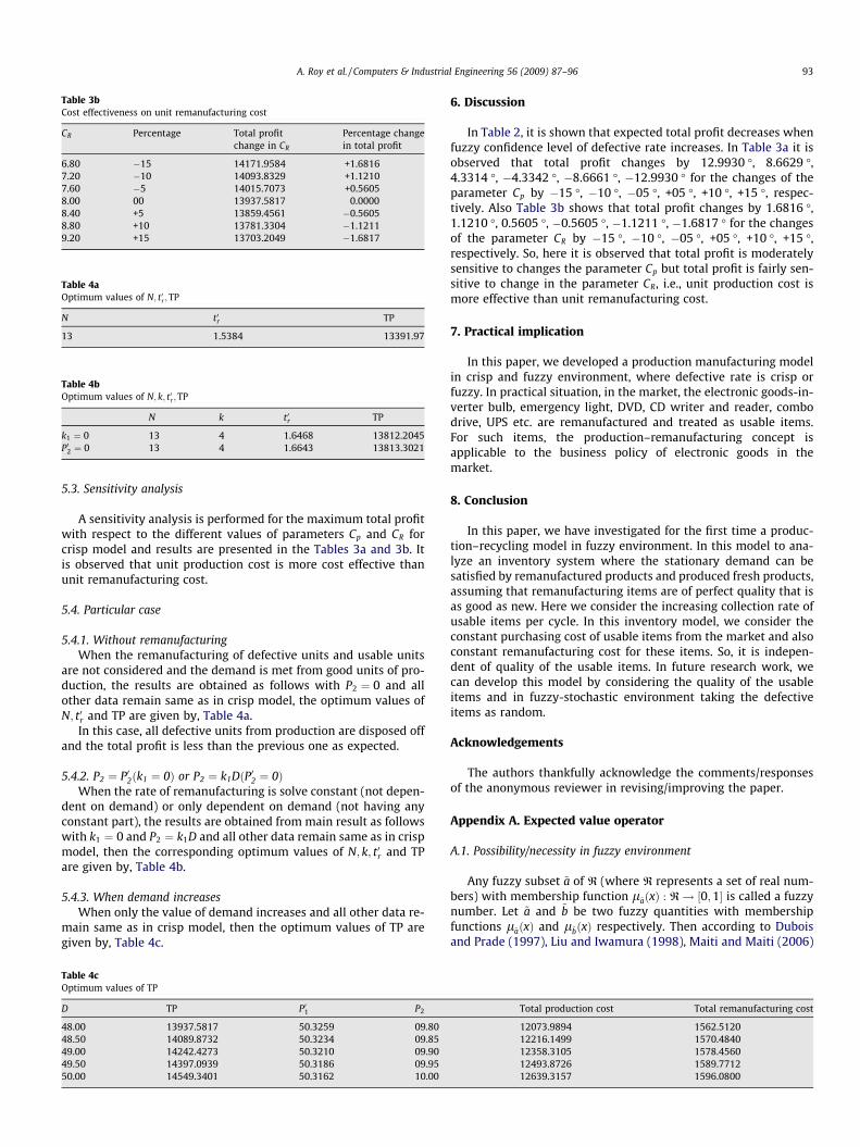
Table 3bCost effectiveness on unit remanufacturing cost

CR Percentage Total profitchange in CR

Percentage changein total profit

6.80 �15 14171.9584 +1.68167.20 �10 14093.8329 +1.12107.60 �5 14015.7073 +0.56058.00 00 13937.5817 0.00008.40 +5 13859.4561 �0.56058.80 +10 13781.3304 �1.12119.20 +15 13703.2049 �1.6817

Table 4bOptimum values of N; k; t0r ;TP

N k t0r TP

k1 ¼ 0 13 4 1.6468 13812.2045P02 ¼ 0 13 4 1.6643 13813.3021

Table 4aOptimum values of N; t0r ;TP

N t0r TP

13 1.5384 13391.97

A. Roy et al. / Computers & Industrial Engineering 56 (2009) 87–96 93

5.3. Sensitivity analysis

A sensitivity analysis is performed for the maximum total profitwith respect to the different values of parameters Cp and CR forcrisp model and results are presented in the Tables 3a and 3b. Itis observed that unit production cost is more cost effective thanunit remanufacturing cost.

5.4. Particular case

5.4.1. Without remanufacturingWhen the remanufacturing of defective units and usable units

are not considered and the demand is met from good units of pro-duction, the results are obtained as follows with P2 ¼ 0 and allother data remain same as in crisp model, the optimum values ofN; t0r and TP are given by, Table 4a.

In this case, all defective units from production are disposed offand the total profit is less than the previous one as expected.

5.4.2. P2 ¼ P02ðk1 ¼ 0Þ or P2 ¼ k1DðP02 ¼ 0ÞWhen the rate of remanufacturing is solve constant (not depen-

dent on demand) or only dependent on demand (not having anyconstant part), the results are obtained from main result as followswith k1 ¼ 0 and P2 ¼ k1D and all other data remain same as in crispmodel, then the corresponding optimum values of N; k; t0r and TPare given by, Table 4b.

5.4.3. When demand increasesWhen only the value of demand increases and all other data re-

main same as in crisp model, then the optimum values of TP aregiven by, Table 4c.

Table 4cOptimum values of TP

D TP P01 P2

48.00 13937.5817 50.3259 09.8048.50 14089.8732 50.3234 09.8549.00 14242.4273 50.3210 09.9049.50 14397.0939 50.3186 09.9550.00 14549.3401 50.3162 10.00

6. Discussion

In Table 2, it is shown that expected total profit decreases whenfuzzy confidence level of defective rate increases. In Table 3a it isobserved that total profit changes by 12.9930 �, 8.6629 �,4.3314 �, �4.3342 �, �8.6661 �, �12.9930 � for the changes of theparameter Cp by �15 �, �10 �, �05 �, +05 �, +10 �, +15 �, respec-tively. Also Table 3b shows that total profit changes by 1.6816 �,1.1210 �, 0.5605 �, �0.5605 �, �1.1211 �, �1.6817 � for the changesof the parameter CR by �15 �, �10 �, �05 �, +05 �, +10 �, +15 �,respectively. So, here it is observed that total profit is moderatelysensitive to changes the parameter Cp but total profit is fairly sen-sitive to change in the parameter CR, i.e., unit production cost ismore effective than unit remanufacturing cost.

7. Practical implication

In this paper, we developed a production manufacturing modelin crisp and fuzzy environment, where defective rate is crisp orfuzzy. In practical situation, in the market, the electronic goods-in-verter bulb, emergency light, DVD, CD writer and reader, combodrive, UPS etc. are remanufactured and treated as usable items.For such items, the production–remanufacturing concept isapplicable to the business policy of electronic goods in themarket.

8. Conclusion

In this paper, we have investigated for the first time a produc-tion–recycling model in fuzzy environment. In this model to ana-lyze an inventory system where the stationary demand can besatisfied by remanufactured products and produced fresh products,assuming that remanufacturing items are of perfect quality that isas good as new. Here we consider the increasing collection rate ofusable items per cycle. In this inventory model, we consider theconstant purchasing cost of usable items from the market and alsoconstant remanufacturing cost for these items. So, it is indepen-dent of quality of the usable items. In future research work, wecan develop this model by considering the quality of the usableitems and in fuzzy-stochastic environment taking the defectiveitems as random.

Acknowledgements

The authors thankfully acknowledge the comments/responsesof the anonymous reviewer in revising/improving the paper.

Appendix A. Expected value operator

A.1. Possibility/necessity in fuzzy environment

Any fuzzy subset ~a of R (where R represents a set of real num-bers) with membership function l~aðxÞ : R! ½0;1� is called a fuzzynumber. Let ~a and ~b be two fuzzy quantities with membershipfunctions l~aðxÞ and l~bðxÞ respectively. Then according to Duboisand Prade (1997), Liu and Iwamura (1998), Maiti and Maiti (2006)

Total production cost Total remanufacturing cost

12073.9894 1562.512012216.1499 1570.484012358.3105 1578.456012493.8726 1589.771212639.3157 1596.0800

94 A. Roy et al. / Computers & Industrial Engineering 56 (2009) 87–96

Posð~a � ~bÞ ¼ fsupðminðl~aðxÞ;l~bðyÞÞ; x; y�R; x � yg ð29ÞNesð~a � ~bÞ ¼ finfðmaxð1� l~aðxÞ;l~bðyÞÞ; x; y�R; x � yg ð30Þ

where the abbreviation ‘Pos’ represents possibility, ‘Nes’ representsnecessity and ‘*’ is any of the relations >;<;¼;6;P.

The dual relationship of possibility and necessity requires that

Nesð~a � ~bÞ ¼ 1� Posð~a � ebÞ ð31Þ

Also necessity measures satisfy the condition

MinðNesð~a � ~bÞ; Nesð~a � ~bÞÞ ¼ 0

The relationships between possibility and necessity measures sat-isfy also the following conditions (cf. Dubois & Prade (1997)):

Posð~a � ~bÞP Nesð~a � ~bÞ;Nesð~a � ~b > 0Þ ) Posð~a � ~bÞ ¼ 1 andPosð~a� ~bÞ < 1) Nesð~a � ~bÞ ¼ 0

If ~a; ~b�R and ~c ¼ f ð~a; ~bÞ where f : R�R! R be a binary opera-tion then membership function l~c of ~c is defined as

l~cðzÞ ¼ supfminðl~aðxÞ;l~bðyÞÞ;x; y�R and z ¼ f ðx; yÞ; 8z�Rg ð32Þ

Recently, based on possibility measure and necessity measure, thethird set function Cr, called credibility measure, analyzed by Liuand Liu (2002) is as follows:

CrðeAÞ ¼ 12½PosðeAÞ þ NesðeAÞ� for any eA in 2R; ð33Þ

where 2R is the power set of R.It is easy to check that Cr satisfies the following conditions:

i* Crð/Þ ¼ 0 and CrðRÞ ¼ 1;ii* CrðeAÞ 6 CrðeBÞ whenever A;B in 2R and A # B;

Thus, Cr is also a fuzzy measure defined on ðR;2RÞ. Besides, Cr isself dual, i.e., CrðeAÞ ¼ 1� CrðeACÞ for any eA in 2R.

In this paper, based on the credibility measure the followingform is defined as

CrðeAÞ ¼ ½qPosðeAÞ þ ð1� qÞNesðeAÞ� ð34Þ

(cf. Liu & Liu (2002))for any eA in 2R and 0 < q < 1. It also satisfiesthe above conditions.

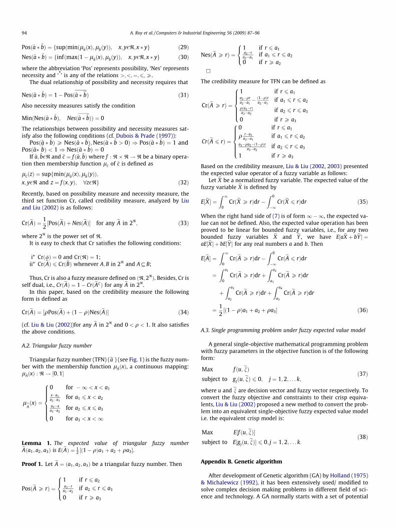
A.2. Triangular fuzzy number

Triangular fuzzy number (TFN) (ea ) (see Fig. 1) is the fuzzy num-ber with the membership function l~AðxÞ, a continuous mapping:l~AðxÞ : R! ½0;1�

leAðxÞ ¼0 for �1 < x < a1

x�a1a2�a1

for a1 6 x < a2

a3�xa3�a2

for a2 6 x 6 a3

0 for a3 < x <1

8>>>>><>>>>>:

Lemma 1. The expected value of triangular fuzzy numbereAða1; a2; a3Þ is EðeAÞ ¼ 12 ½ð1� qÞa1 þ a2 þ qa3�.

Proof 1. Let eA ¼ ða1; a2; a3Þ be a triangular fuzzy number. Then

PosðeA P rÞ ¼1 if r 6 a2a3�r

a3�a2if a2 6 r 6 a3

0 if r P a3

8><>:

NesðeA P rÞ ¼1 if r 6 a1a2�r

a2�a1if a1 6 r 6 a2

0 if r P a2

8<:h

The credibility measure for TFN can be defined as

CrðeA P rÞ ¼

1 if r 6 a1a2�qra2�a1

� ð1�qÞra2�a1

if a1 6 r 6 a2

qða3�rÞa3�a2

if a2 6 r 6 a3

0 if r P a3

8>>>><>>>>:CrðeA 6 rÞ ¼

0 if r 6 a1

q r�a1a2�a1

if a1 6 r 6 a2

a3�qa2�ð1�qÞra3�a2

if a2 6 r 6 a3

1 if r P a3

8>>>><>>>>:Based on the credibility measure, Liu & Liu (2002, 2003) presentedthe expected value operator of a fuzzy variable as follows:

Let eX be a normalized fuzzy variable. The expected value of thefuzzy variable eX is defined by

E½eX � ¼ Z 1

0CrðeX P rÞdr �

Z 0

�1CrðeX 6 rÞdr ð35Þ

When the right hand side of (7) is of form1�1, the expected va-lue can not be defined. Also, the expected value operation has beenproved to be linear for bounded fuzzy variables, i.e., for any twobounded fuzzy variables eX and eY , we have E½aeX þ beY � ¼aE½eX � þ bE½eY � for any real numbers a and b. Then

E½eA� ¼ Z 1

0CrðeA P rÞdr �

Z 0

�1CrðeA 6 rÞdr

¼Z a1

0CrðeA P rÞdr þ

Z a2

a1

CrðeA P rÞdr

þZ a3

a2

CrðeA P rÞdr þZ a4

a3

CrðeA P rÞdr

¼ 12½ð1� qÞa1 þ a2 þ qa3� ð36Þ

A.3. Single programming problem under fuzzy expected value model

A general single-objective mathematical programming problemwith fuzzy parameters in the objective function is of the followingform:

Max f ðu; enÞsubject to gjðu; enÞ 6 0; j ¼ 1;2; . . . k;

ð37Þ

where u and en are decision vector and fuzzy vector respectively. Toconvert the fuzzy objective and constraints to their crisp equiva-lents, Liu & Liu (2002) proposed a new method to convert the prob-lem into an equivalent single-objective fuzzy expected value modeli.e. the equivalent crisp model is:

Max E½f ðu; enÞ�subject to E½gjðu; enÞ� 6 0; j ¼ 1;2; . . . k:

ð38Þ

Appendix B. Genetic algorithm

After development of Genetic algorithm (GA) by Holland (1975)& Michalewicz (1992), it has been extensively used/ modified tosolve complex decision making problems in different field of sci-ence and technology. A GA normally starts with a set of potential

A. Roy et al. / Computers & Industrial Engineering 56 (2009) 87–96 95

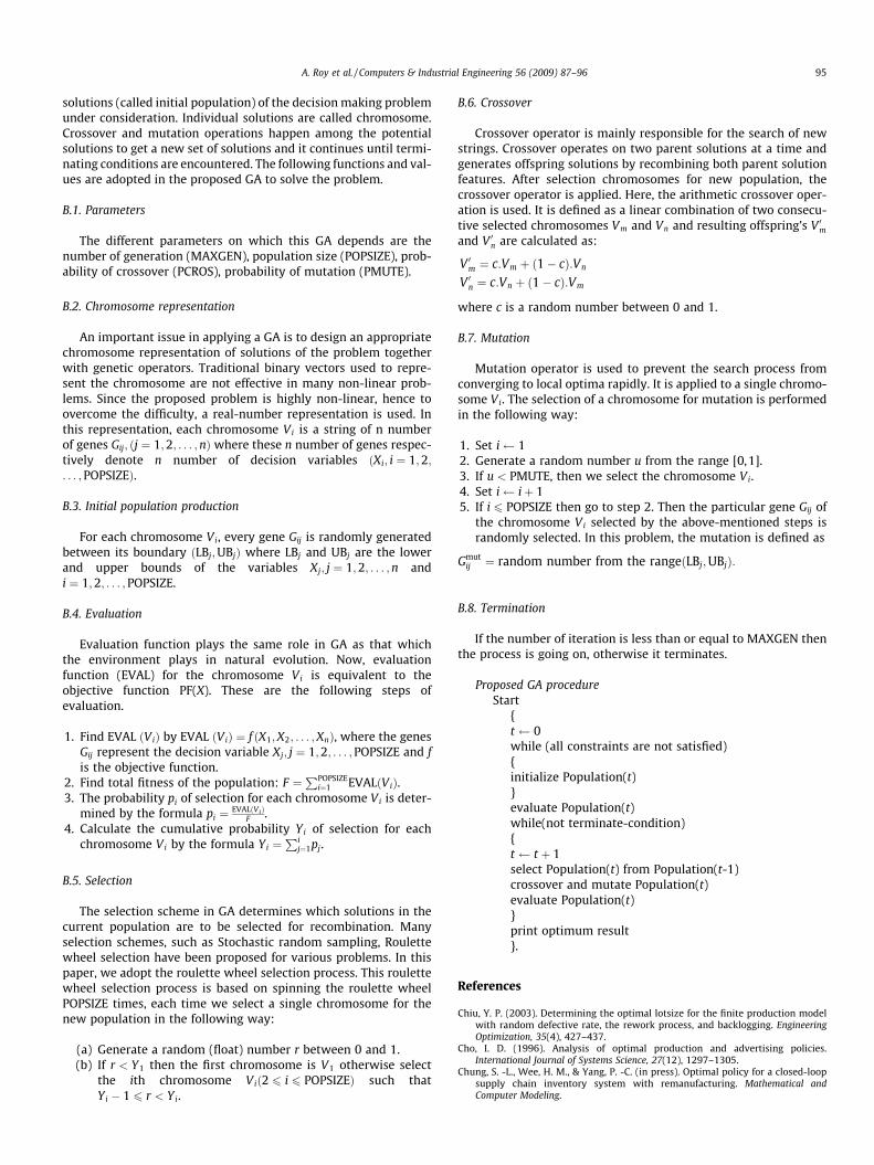
solutions (called initial population) of the decision making problemunder consideration. Individual solutions are called chromosome.Crossover and mutation operations happen among the potentialsolutions to get a new set of solutions and it continues until termi-nating conditions are encountered. The following functions and val-ues are adopted in the proposed GA to solve the problem.

B.1. Parameters

The different parameters on which this GA depends are thenumber of generation (MAXGEN), population size (POPSIZE), prob-ability of crossover (PCROS), probability of mutation (PMUTE).

B.2. Chromosome representation

An important issue in applying a GA is to design an appropriatechromosome representation of solutions of the problem togetherwith genetic operators. Traditional binary vectors used to repre-sent the chromosome are not effective in many non-linear prob-lems. Since the proposed problem is highly non-linear, hence toovercome the difficulty, a real-number representation is used. Inthis representation, each chromosome Vi is a string of n numberof genes Gij; ðj ¼ 1;2; . . . ;nÞ where these n number of genes respec-tively denote n number of decision variables ðXi; i ¼ 1;2;. . . ;POPSIZEÞ.

B.3. Initial population production

For each chromosome Vi, every gene Gij is randomly generatedbetween its boundary ðLBj;UBjÞ where LBj and UBj are the lowerand upper bounds of the variables Xj; j ¼ 1;2; . . . ;n andi ¼ 1;2; . . . ;POPSIZE.

B.4. Evaluation

Evaluation function plays the same role in GA as that whichthe environment plays in natural evolution. Now, evaluationfunction (EVAL) for the chromosome Vi is equivalent to theobjective function PF(X). These are the following steps ofevaluation.

1. Find EVAL ðViÞ by EVAL ðViÞ ¼ f ðX1;X2; . . . ;XnÞ, where the genesGij represent the decision variable Xj; j ¼ 1;2; . . . ;POPSIZE and fis the objective function.

2. Find total fitness of the population: F ¼PPOPSIZE

i¼1 EVALðViÞ.3. The probability pi of selection for each chromosome Vi is deter-

mined by the formula pi ¼ EVALðViÞF .

4. Calculate the cumulative probability Yi of selection for eachchromosome Vi by the formula Yi ¼

Pij¼1pj.

B.5. Selection

The selection scheme in GA determines which solutions in thecurrent population are to be selected for recombination. Manyselection schemes, such as Stochastic random sampling, Roulettewheel selection have been proposed for various problems. In thispaper, we adopt the roulette wheel selection process. This roulettewheel selection process is based on spinning the roulette wheelPOPSIZE times, each time we select a single chromosome for thenew population in the following way:

(a) Generate a random (float) number r between 0 and 1.(b) If r < Y1 then the first chromosome is V1 otherwise select

the ith chromosome Við2 6 i 6 POPSIZEÞ such thatYi � 1 6 r < Yi.

B.6. Crossover

Crossover operator is mainly responsible for the search of newstrings. Crossover operates on two parent solutions at a time andgenerates offspring solutions by recombining both parent solutionfeatures. After selection chromosomes for new population, thecrossover operator is applied. Here, the arithmetic crossover oper-ation is used. It is defined as a linear combination of two consecu-tive selected chromosomes Vm and Vn and resulting offspring’s V 0mand V 0n are calculated as:

V 0m ¼ c:Vm þ ð1� cÞ:Vn

V 0n ¼ c:Vn þ ð1� cÞ:Vm

where c is a random number between 0 and 1.

B.7. Mutation

Mutation operator is used to prevent the search process fromconverging to local optima rapidly. It is applied to a single chromo-some Vi. The selection of a chromosome for mutation is performedin the following way:

1. Set i 12. Generate a random number u from the range [0,1].3. If u < PMUTE, then we select the chromosome Vi.4. Set i iþ 15. If i 6 POPSIZE then go to step 2. Then the particular gene Gij of

the chromosome Vi selected by the above-mentioned steps israndomly selected. In this problem, the mutation is defined as

Gmutij ¼ random number from the rangeðLBj;UBjÞ:

B.8. Termination

If the number of iteration is less than or equal to MAXGEN thenthe process is going on, otherwise it terminates.

Proposed GA procedure

Start

{t 0while (all constraints are not satisfied){initialize Population(t)}evaluate Population(t)while(not terminate-condition){t t þ 1select Population(t) from Population(t-1)crossover and mutate Population(t)evaluate Population(t)}print optimum result}.

References

Chiu, Y. P. (2003). Determining the optimal lotsize for the finite production modelwith random defective rate, the rework process, and backlogging. EngineeringOptimization, 35(4), 427–437.

Cho, I. D. (1996). Analysis of optimal production and advertising policies.International Journal of Systems Science, 27(12), 1297–1305.

Chung, S. -L., Wee, H. M., & Yang, P. -C. (in press). Optimal policy for a closed-loopsupply chain inventory system with remanufacturing. Mathematical andComputer Modeling.

96 A. Roy et al. / Computers & Industrial Engineering 56 (2009) 87–96

Dey, J. K., Kar, S., & Maiti, M. (2005). An iterative method for inventory control withfuzzy-lead time. European Journal of Operational Research, 167, 381–397.

Dobos, I. (2003). Optimal production-inventory strategies for a HMMS-type reverselogistics system. International Journal of Production Economics, 81, 351–360.

Dubois, D., & Prade, H. (1988). Possibility Theory. New York, London.Dubois, D., & Prade, H. (1997). The three semantics of fuzzy sets. Fuzzy Sets and

Systems, 90, 141–150.Dobos, I., & Richter, K. (2004). An extended production/recycling model with

stationary demand and return rates. International Journal of ProductionEconomics, 90, 311–323.

Dobos, I., & Richter, K. (2006). A production/recycling model with qualityconsideration. International Journal of Production Economics, 104, 571–579.

Fleischmann, M., Bloemhof-Runwaard, J. M., Dekker, R., Van der Lann, E., Numen, J.A. E. E. van, & Wassenhove, L. N. van (1997). Quantitative models for reverselogistics, A review, European Journal of Operational Research 103, 1–17.

Guide, V. D. R., Jayaraman, V., Srivastava, R., & Benton, W.C. (1998). Supply chainmanagement for recoverable manufacturing systems, Suffolk University workingpaper 98/101/OM.

Gupta, S. M., & Gungor, A. (1999). Issues in environmentally consciousmanufacturing and product recovery. Computers and Industrial Engineering, 36,190–194.

Hayek, P., & Salameh, M. K. (2001). Production lot sizing with the reworking ofimperfect quality items produced. Production Planning and Control, 12(6),437–584.

Holland, H. J. (1975). Adaptation in natural and artificial systems. University ofMichigan.

Koh, S.-G., Hwang, H., Sohn, K.-I., & Ko, C.-S. (2002). An optimal ordering andrecovery policy for reusable items. Computers and Industrial Engineering, 43,59–73.

Liu, B., & Iwamura, K. B. (1998). Chance constraint programming with fuzzyparameters. Fuzzy Sets and Systems, 94, 227–237.

Liu, B., & Liu, Y. K. (2002). Expected value of Fuzzy variable and Fuzzy expectedvalue Models. IEEE Transactions of Fuzzy Systems, 10(4), 445–450.

Liu, Y. K., & Liu, B. A. (2003). Class of fuzzy random optimization: expected valuemodels. Information Science, 155, 89–102.

Maiti, M. K., & Maiti, M. (2006). Fuzzy inventory model with two warehouses underpossibility constraints. Fuzzy Sets and Systems, 157, 52–73.

Maity, K., & Maiti, M. (2005). Numerical approach of multi-objective optimal controlproblem in imprecise environment. Fuzzy Optimization and Decision Making, 4,313–330.

Michalewicz, Z. (1992). Genetic Algorithms + data structures = evolution programs.Berlin: Springer.

Richter, K. (1996a). The EOQ repair and waste disposal model withvariable setup numbers. European Journal of Operational Research, 96,313–324.

Richter, K. (1996b). The extended EOQ repair and waste disposal model.International Journal of Production Economics, 45, 443–447.

Richter, K. (1997). Pure and mixed strategies for the EOQ repair and waste disposalproblem. OR Spectrum, 19, 123–129.

Richter, K., & Dobos, I. (1999). Analysis of the EOQ repair and waste disposalproblem with integer setup numbers. International Journal of ProductionEconomics, 59, 463–467.

Sana, S., Goyal, S. K., & Chaudhuri, K. S. (2004). A production–inventory model for adeteriorating item with trended demand and shortages. European Journal ofOperational Research, 157, 357–371.

Wang, J., & Shu, Y. F. (2005). Fuzzy decision modelling for supply chainmanagement. Fuzzy Sets and Systems, 150, 107–127.

Wee, H. M., Yu, J., Lo, C.-C., & Chen, K. L. (2005). Multiple replenishment inventorymodel for reusable product with imperfect quality. Journal of Management andSystems, 12(3), 89–107.

Wee, H. M., Lo, C. -C., & Hsu, P. -H. (accepted). A multi-objective joint replenishmentinventory model of deteriorated items in a fuzzy environment. European Journalof Operational Research (SCI).

Wee, H. M., Yu, J. C. P., Su, L. -H., & Wu, T. -C. (2006b). Optimal ordering and recoverypolicy for reusable items with shortages. Lecture Notes in Computer Science, LNCS4247, 284–291.

Wee, H. M., Yu, J., & Chen, M. C. (2007). Optimal inventory model for items withimperfect quality and shortage backordering. Omega, 35, 7–11.

Wee, H. M., & Chung, C. J. (2008). Optimizing replenishment policy for anintegrated production inventory deteriorating model considering greencomponent-value design and remanufacturing. Journal of Production Research,iFirst (SCI), 1–26.

Zadeh, L. A. (1978). Fuzzy sets as a basis for a theory of possibility. Fuzzy Sets andSystems, 1, 3–28.