This preprint is originally revised and extended from its previous version (https://arxiv.org/abs/2101.06580v1), sothere may exist some overlaps. However, due to significant differences, both are kept separately on ArXiv. It isrecommended to read and make use of these two preprints complementarily. Please cite this paper as:Shi, Rongye, et al.“A Physics-Informed Deep Learning Paradigm for Traffic State and Fundamental DiagramEstimation.” IEEE Transactions on Intelligent Transportation Systems (2021). DOI: 10.1109/TITS.2021.3106259

1

A Physics-Informed Deep Learning Paradigm forTraffic State and Fundamental Diagram Estimation

Rongye Shi, Member, IEEE, Zhaobin Mo, Kuang Huang, Xuan Di, Member, IEEE, and Qiang Du

Abstract—Traffic state estimation (TSE) bifurcates into twocategories, model-driven and data-driven (e.g., machine learning,ML), while each suffers from either deficient physics or smalldata. To mitigate these limitations, recent studies introduced ahybrid paradigm, physics-informed deep learning (PIDL), whichcontains both model-driven and data-driven components. Thispaper contributes an improved version, called physics-informeddeep learning with a fundamental diagram learner (PIDL+FDL),which integrates ML terms into the model-driven componentto learn a functional form of a fundamental diagram (FD),i.e., a mapping from traffic density to flow or velocity. Theproposed PIDL+FDL has the advantages of performing the TSElearning, model parameter identification, and FD estimationsimultaneously. We demonstrate the use of PIDL+FDL to solvepopular first-order and second-order traffic flow models andreconstruct the FD relation as well as model parameters that areoutside the FD terms. We then evaluate the PIDL+FDL-basedTSE using the Next Generation SIMulation (NGSIM) dataset.The experimental results show the superiority of the PIDL+FDLin terms of improved estimation accuracy and data efficiency overadvanced baseline TSE methods, and additionally, the capacityto properly learn the unknown underlying FD relation.

Index Terms—Traffic state estimation, fundamental diagramlearner, physics-informed deep learning.

I. INTRODUCTION

TTRAFFIC state estimation (TSE) refers to the datamining problem of reconstructing traffic state variables,

including but not limited to flow, density, and speed, on roadsegments using partially observed data from traffic sensors [1].TSE approaches can be briefly divided into two main cat-egories: model-driven and data-driven [2]. A model-drivenapproach is based on a priori knowledge of traffic dynamics,usually described by a physical model, e.g., the Lighthill-Whitham-Richards (LWR) model [3], [4] and Aw-Rascle-Zhang (ARZ) model [5], [6], to estimate the traffic state usingpartial observation. It assumes the model to be representativeof the real-world traffic dynamics such that the unobservedvalues can be properly added using the model with small data.The disadvantage is that existing models, which are providedby different modelers, may only capture limited dynamics of

Manuscript received March 19, 2020; revised November 9, 2020, January23, 2021, June 5, 2021 and August 17, 2021; accepted August 17, 2021.(Corresponding author: Xuan Di.)

Rongye Shi, Zhaobin Mo, and Xuan Di are with the Department of CivilEngineering and Engineering Mechanics, Columbia University, New York,NY, 10027 USA (e-mail: rongyes@alumni.cmu.edu; zm2302@columbia.edu;sharon.di@columbia.edu).

Kuang Huang and Qiang Du are with the Department of Applied Physicsand Applied Mathematics, Columbia University, New York, NY, 10027 USA(e-mail: kh2862@columbia.edu; qd2125@columbia.edu).

Xuan Di and Qiang Du are also with the Data Science Institute, ColumbiaUniversity, New York, NY, 10027 USA.

the real-world traffic, resulting in low-quality estimation inthe case of inappropriately-chosen models and poor modelcalibrations. Paradoxically, sometimes, verifying or calibratinga model requires a large amount of observed data, underminingthe data efficiency of model-driven approaches.

A data-driven approach is to infer traffic states based onthe dependence learned from historical data using statisticalor machine learning (ML) methods. Approaches of this typedo not use any explicit traffic models or other theoreticalassumptions, and can be treated as a “black box” with no in-terpretable and deductive insights. The disadvantage is that inorder to maintain a good generalizable inference to long-termunobserved values, massive and representative historical dataare a prerequisite, leading to high demands on data collectioninfrastructure and enormous installation-maintenance costs.

To mitigate the limitations of the above-mentioned TSEapproaches, hybrid TSE methods are introduced, which inte-grate the traffic knowledge in the form of traffic flow modelsto ML models for TSE. The hybrid methods based on thelearning paradigm of physics-informed deep learning (PIDL)are gaining increasing attentions in recently years, and is thefocus of this paper. PIDL contains both a model-driven com-ponent (a physics-informed neural network for regularization)and a data-driven component (a physics-uninformed neuralnetwork for estimation), making possible the integration ofthe strengths of both model-driven and data-driven approacheswhile overcoming the weaknesses of either.

Despite that the addition of physics could guide the trainingof PIDL efficiently, complicated mathematical formulas couldinstead make the PIDL difficult to train. There are manytheoretical attempts made to add sophistication (usually in theform of complicated terms) to the FD relation for an improveddescription of the dynamics. To balance the sophisticationand trainability of encoding physics, this paper explores apromising direction by approximating the FD relation withan ML surrogate, instead of hard-encoding an FD equation.Following this direction, we introduce an improved PIDLparadigm, called physics-informed deep learning with a fun-damental diagram learner (PIDL+FDL), which integrates anML surrogate (e.g., an NN) into the model-driven componentto represent the fundamental diagram (FD) and estimate theFD relation. We focus on highway TSE with observed datafrom loop detectors, using traffic density or velocity as trafficvariables. Our contributions are:

• We propose the PIDL+FDL-based TSE method that pos-sesses advantages to

- Perform the TSE with improved estimation accuracy:A proper integration of ML surrogates may avoid directly

arX

iv:2

106.

0314

2v4

[cs

.LG

] 2

1 Se

p 20

21

2

encoding the complicated terms in PIDL and trade offbetween the sophistication of the model-driven aspect ofPIDL and the training flexibility, making the frameworka better fit to the TSE problem;

- Perform the FD estimation: The PIDL+FDL uses anML surrogate to directly learn the underlying FD relationwithout any FD output measurements, i.e., the ML surro-gate is purely trained under physical regularization fromPIDL, making it more likely to learn a suitable relationalong with the TSE training. It can also get around thecalibration of parameters inside the FD equation;

- Perform the model parameter identification: For acomplete traffic model reconstruction, in addition to theFD estimation, there may exist model parameters outsidethe FD terms to be learned. The proposed PIDL+FDLconducts the model parameter identification jointly.

• We validate the PIDL+FDL performance with both nu-merical experiments and real-world data: To demon-strate the strengths of the PIDL+FDL, we design thePIDL+FDL architectures for the traffic dynamics gov-erned by the Greenshields-based LWR and ARZ models,respectively. Additionally, experiments using the real-world data, the Next Generation SIMulation (NGSIM)dataset, are conducted. The experimental results show theadvantages of PIDL in terms of estimation accuracy anddata efficiency over baselines and the capacity to properlyestimate the FD relation and model parameters.

The rest of this paper is organized as follows. Section IIbriefs related work on TSE and PIDL. Section III formalizesthe PIDL+FDL framework for TSE. Sections IV and V detailthe designs and experiments of PIDL+FDL for Greenshields-based LWR and Greenshields-based ARZ, respectively. Sec-tion VI evaluates the PIDL+FDL on NGSIM data over base-lines. Section VII concludes our work.

II. RELATED WORK OF TRAFFIC STATE ESTIMATION

Most model-driven estimation approaches are data assimila-tion (DA) based, which find “the most likely state,” allowingobservation to correct models’ prediction. Popular examplesinclude the Kalman filter (KF) and its variants [7], [8]. Otherthan KF-like methods, particle filter (PF) [9] with improvednonlinear representation, adaptive smoothing filter (ASF) [10]for combining multiple sensing data, were proposed to im-prove and extend different aspects of the TSE process. Indata-driven approaches, to handle complicated traffic data, MLapproaches were involved, including long short term memory(LSTM) and deep embedded models [11], [12].

A paradigm integrating physics to ML has gained increasinginterests recently. Yuan et al [13] proposed a physics regular-ized Gaussian processfor macroscopic traffic flow modelingand TSE. The hybrid methods using the PIDL framework [14],[15] is becoming an active field. Huang et al [16] studiedthe use of PIDL to encode the Greenshields-based LWRand validated it in the loop detector scenarios using SUMOsimulated data. Barreau et al [17], [18], [19] studied the probevehicle sensors and developed coupled micro-macro modelsfor PIDL to perform TSE. Shi et al [20] extended the PIDL-

based TSE to the second-order ARZ with observed data fromboth loop detectors and probe vehicles.

We want to highlight that, as to model reconstruction, whichis another feature of PIDL-based TSE, this paper only assumesa traffic flow conservation equation and optionally, a momen-tum equation for the velocity field, without specifying anymathematical relation between traffic quantities. While [17],[19] directly fit a velocity function using measured densityand velocity from probe vehicles before or during the PIDLtraining, we, in this paper, focus on a more general case, wherethe output of the FD function is unobserved from sensors,and the end-to-end FD relation is learned directly using MLsurrogates under the PIDL framework. In summary, this papercontributes to the trend of developing hybrid methods for TSEand model reconstruction, especially with both FD estimationand model parameter identification involved.

III. MATHEMATICAL SETTING FOR PIDL+FDL

This section introduces the PIDL+FDL framework in thecontext of TSE at a high level.

A. PIDL for TSE

Consider a traffic flow dynamics of a road segment thatis governed by a set of non-linear equations (e.g., partialdifferential equations, PDEs):

N (MMM(t, x),QQQ;λλλ) = 000, x ∈ [0, L], t ∈ [0, T ], (1)

where L ∈ R+, T ∈ R+. We use bold symbols to denote vec-tors by default. The operator N contains the governing non-linear equations of the traffic flow dynamics, while MMM(t, x)contains the traffic state variables, such as the traffic densityρ(t, x) and velocity u(t, x). λλλ contains the model parameters.The model includes intermediate unobserved traffic variablesQQQ that have some hidden relationship with MMM(t, x). Thus, thedynamics can be represented by

N (MMM,QQQ(MMM);λλλ) = 000, (2)

and MMM stands for MMM(t, x). For general discussion, the valuesofQQQ are not assumed to be directly observable, and the relationis either unknown or deduced based on assumptions whichmay be deficient. The TSE problem is to reconstruct the trafficstates MMM at each point (t, x) in a continuous domain frompartial observation of MMM . Accordingly, the continuous spatio-temporal domain D is a set of points: D = {(t, x)|∀t ∈[0, T ], x ∈ [0, L]}. We represent this continuous domain ina discrete manner using grid points G ∈ D that are evenlydeployed throughout the domain. We define the set of gridpoints as G = {(t(r), x(r))|r = 1, .., Ng}. The total numberof grid points, Ng , controls the fine-grained level of G as arepresentation of the continuous domain.

PIDL approximates MMM(t, x) using a neural network withtime t and location x as its inputs. This neural network iscalled physics-uninformed neural network (PUNN) (or esti-mation network in our TSE study), which is parameterizedby θ. We denote the approximation of MMM(t, x) from PUNNas MMM(t, x; θ). When N , QQQ and λλλ are known, during the

3

learning phase of PUNN (i.e., to find the optimal θ for PUNN),the following equiation defines the residual values of theapproximation MMM(t, x; θ):

fff(t, x; θ) := N (MMM(t, x; θ),QQQ(MMM(t, x; θ));λλλ), (3)

which is designed according to the traffic flow model inEq. (2). The calculation of residual fff(t, x; θ) is done by aphysics-informed neural network (PINN). This network cancompute fff(t, x; θ) directly using MMM(t, x; θ), the output ofPUNN, as its input. When MMM(t, x; θ) is closer to the true valueMMM(t, x), the residual fff will be closer to 000. PINN introducesno new parameters, and thus, shares the same θ of PUNN.

In most cases, even the model is given, the model param-eters λλλ are unknown and can be made as learning variablesin PINN for model parameter identification. The residual fff isthen redefined as

fff(t, x; θ,λλλ) := N (MMM(t, x; θ),QQQ(MMM(t, x; θ));λλλ). (4)

This paper assumes unknown model parameters by default.In PINN, fff(t, x; θ,λλλ) is calculated by automatic differ-

entiation technique, which can be done by the functiontf.gradient in Tensorflow. The activation functions and theconnecting structure of neurons in PINN are designed toconduct the differential operation in Eq. (4). We would liketo emphasize that, the connecting weights in PINN have fixedvalues which are determined by the traffic flow model andλλλ are encoded as learning variables. Thus, the residual fff isparameterized by both θ and λλλ.

The training data for PIDL consist of (1) observation pointsO = {(t(i)o , x

(i)o )|i = 1, ..., No}, (2) target values P =

{MMM (i)|i = 1, ..., No} (i.e., the true traffic states at the obser-vation points), and (3) auxiliary points A = {(t(j)a , x

(j)a )|j =

1, ..., Na}. i and j are the indexes of observation points andauxiliary points, respectively. One target value is associatedwith one observation point, and thus, O and P have the sameindexing system (indexed by i). This paper uses the term,observed data, to denote {O,P}. Both O and A are subsetsof the grid points G (i.e., O ∈ G and A ∈ G).

Observation points O are limited to the time and locationsthat traffic sensors can visit and record. In contrast, auxiliarypoints A have neither measurement requirements nor locationlimitations, and the number of A is controllable. A are usedfor regularization purposes, and this is why they are called“auxiliary”. To train a PUNN for TSE, the loss is used:

Lossθ,λλλ = α ·MSEo + β ·MSEa

= α · 1

No

No∑i=1

|MMM(t(i)o , x(i)o ; θ)−MMM (i)|2︸ ︷︷ ︸data discrepancy

+β · 1

Na

Na∑j=1

|fff(t(j)a , x(j)a ; θ,λλλ)|2︸ ︷︷ ︸physical discrepancy

.

(5)

where α and β are hyperparameters for balancing the con-tribution to the loss made by data discrepancy and physicaldiscrepancy, respectively. The data discrepancy is defined asthe mean square error (MSE) between approximation MMM onO and target values P . The physical discrepancy is the MSEbetween residual values on A and 000, quantifying the extent towhich the approximation deviates from the traffic model.

Given the training data, we apply neural network trainingalgorithms to solve (θ∗,λλλ∗) = argminθ,λλλ Lossθ,λλλ. Then, theλλλ∗-parameterized traffic flow model of Eq. (4) is the mostlikely physics that generates the observed data, and the θ∗-parameterized PUNN can then be used to approximate thetraffic states on G, which are consistent with the reconstructedtraffic flow model in Eq. (2).

B. PIDL + FDL for TSE

As has been discussed previously, the PIDL-based TSEmethods may perform poorly when informed by a highlysophisticated traffic flow model. This is because the mod-els may contain complicated terms that are unfriendly todifferentiation-based learning (e.g., square root operators oflearning variables in the denominator, etc.), making the train-ing and performance very sensitive to the structural designof PINN. Many efforts such as variable conversion, decom-position and factorization need to be made to have the PINNtrainable and the loss to converge. In our framework of Eq.(2),these “unfriendly” terms can be contained as part of the hiddenrelation QQQ. To address the issues of PIDL-based TSE, wepropose to use an ML surrogate QQQ to directly represent theQQQ and learn the relation under the PIDL framework, insteadof hard-encoding a complicated term in PINN.

The advantages of properly introducing an ML surrogateof QQQ are two-fold: (1) An ML term is usually differentiation-friendly, giving the PIDL more flexibility to achieve an im-proved TSE accuracy. (2) No assumptions are made to thehidden relation, and it is possible to learn a more suitable QQQwhen trained under the physical regularization from PINN.

This paper focuses on one kind of hidden relationships, thefundamental diagram (FD), and the corresponding learningparadigm is called PIDL with an FD Learner (PIDL+FDL).Specifically, the FD Learner, formalized as QQQ(MMM ;ω), can bedesigned as a neural network parameterized by ω to representthe unknown FD relation, which takes the estimated trafficvariables MMM(t, x; θ) as its input. The residual of Eq.(4) isredefined as the following

fff(t, x; θ, ω,λλλ) := N (MMM(t, x; θ), QQQ(MMM(t, x; θ);ω);λλλ). (6)

The loss function becomes

Lossθ,ω,λλλ = α ·MSEo + β ·MSEa

= α · 1

No

No∑i=1

|MMM(t(i)o , x(i)o ; θ)−MMM (i)|2

+β · 1

Na

Na∑j=1

|fff(t(j)a , x(j)a ; θ, ω,λλλ)|2.

(7)

4

Using the training data, we apply neural network trainingalgorithms to solve (θ∗, ω∗,λλλ∗) = argminθ,ω,λλλ Lossθ,ω,λλλ.Then, in addition to TSE learning and model parameteridentification, the FD estimation is conducted automatically.The ω∗-parameterized QQQ can be used to represent the unknownhidden fundamental diagram relation. Note that the values ofQQQ are not assumed to be observable, and thus, are not part ofthe data (i.e., to directly learn the QQQ from data cannot apply).

In some cases, the curve of the learned QQQ may presentabnormal shapes on edge conditions. To mitigate this, onecan encode prior knowledge into the loss as an additionalregularization term Reg(QQQ) to reshape the FD. As an example,we can use QQQ to represent the density-flow relation, i.e., theflux function (one typical kind of FD), mapping the density ρto the flow value, which is denoted as a scalar Q(ρ). Existingtheoretical works usually assume Q to be concave with respectto the traffic density ρ. To impose the concavity property, wedesign the following regularization term:

Reg(Q) =

∫ b

a

max(0,∂2Q(ρ)

∂ρ2)dρ, (8)

where the hyperparameters a and b determine the interval ofρ on which the reshaping takes effects without interfering thelearning on other regions. We propose this design becausemost abnormal shapes only occur on edge region and it is notnecessary to regularize over the whole traffic density domain.We apply Lossθ,ω,λλλ = α ·MSEo+β ·MSEa+ξ ·Reg(Q) inthe learning phase and properly reshape the learned FD curves.

IV. PIDL+FDL FOR GREENSHIELDS-BASED LWR

The first numerical example aims to show the capability ofour method to estimate the traffic dynamics governed by theLWR model with a Greenshields flux function.

Define flow rate Q (a scalar) to be the number of vehiclespassing a specific position on the road per unit time, andtraffic density ρ to be the average number of vehicles perunit length of the road. The traffic flux Q(ρ) describes Q asa function of ρ, which is the FD relation of interest in thisnumerical example. We treat ρ as the basic traffic state variableto estimate. Greenshields flux is a basic and popular choiceof Q(ρ), which is defined as Q(ρ) = ρumax(1 − ρ/ρmax),where umax and ρmax are maximum velocity and maximum(jam) density, respectively. This flux function has a quadraticform with two coefficients umax and ρmax.

The LWR model [3], [4] describes the macroscopic trafficflow dynamics as ρt + (Q(ρ))x = 0, which is derived froma conservation law of vehicles. In order to reproduce morephenomena in observed traffic data, such as delayed drivingbehaviors due to drivers’ reaction time, diffusively correctedLWRs were introduced, by adding a diffusion term, containinga second-order derivative ρxx. We focus on one version of thediffusively corrected LWRs: ρt + (Q(ρ))x = ερxx, where ε isthe diffusion coefficient.

In this section, we study the Greenshields-based LWR trafficflow model of a “ring road”:

ρt + (Q(ρ))x = ερxx, t ∈ [0, 3], x ∈ [0, 1],

Q(ρ) = ρ · umax(1− ρ

ρmax

)(FD relation),

ρ(t, 0) = ρ(t, 1) (boundary condition 1),

ρx(t, 0) = ρx(t, 1) (boundary condition 2),

(9)

where ρmax = 1.0, umax = 1.0, and ε = 0.005. ρmax andumax are usually determined by physical restrictions of theroad and vehicles.

Given the bell-shaped initial 0.1+0.8e−( x−0.50.2 )2 , x ∈ [0, 1],

we apply the Godunov scheme to solve Eqs. (9) on 960 (time)× 240 (space) grid points G evenly deployed throughout the[0, 3] × [0, 1] domain. In this case, the total number of gridpoints G is Ng =960×240. The numerical solution is shownin Fig. 2 (see the heat map background). From the figure, wecan visualize the dynamics as follows: At t = 0, there is a peakdensity at the center of the road segment, and this peak evolvesto propagate along the direction of x, which is known as thephenomenon of traffic shockwave. Since this is a ring road, theshockwave reaching x = 1 continues at x = 0. This numericalsolution of the Greenshields-based LWR model is treated asthe ground-truth traffic density. We will apply a PIDL+FDL-based approach method to estimate the entire traffic densityfield using observed data as well as to estimate the FD relationand model parameters.

A. PIDL+FDL Architecture Design

The authors’ previous work [20] has shown the capacity ofPIDL to perform both TSE and model parameter identificationwhen the closed traffic flow model is given. Here we areonly given the knowledge of conservation law and boundaryconditions, i.e., the FD relation is unknown and no directobservation of Q is available.

We employ a neural network Q(·;ω) to estimate the trafficflow from the traffic density and to represent the FD relationof interest. Based on Eqs. (9), we define the residual value ofPUNN’s traffic density estimation ρ(t, x; θ) as

f(t, x; θ, ω, ε) := ρt(t, x; θ)+(Q(ρ(t, x; θ);ω))x−ερxx(t, x; θ).(10)

Note that the parameter λλλ contains the coefficient ε only.Given the definition of f , the corresponding PIDL+FDL

architecture is shown in Fig. 1. This architecture consistsof a PUNN for traffic density estimation, followed by aPINN+FD Learner for calculating the residual Eq. (10). ThePUNN parameterized by θ is designed as a fully-connectedfeedforward neural network with 8 hidden layers and 20hidden nodes in each hidden layer. Hyperbolic tangent function(tanh) is used as the activation function for each hidden neuronin PUNN. In contrast, in PINN, connecting weights are fixedand the activation function of each node is designed to conductspecific nonlinear operation for calculating an intermediate(hidden) value of f . The flow value is calculated by a separateneural network Q(ρ;ω) with two hidden layers and 20 hiddennodes for each. The model parameter ε is held by a variablenode (blue rectangular nodes).

5

...

...

...

...

...

...

x

tˆ ( , ; )t x

...

ˆxx

ˆt

ˆ ˆ( ( ))xQ f

PINN+FD Learner

PUNN

(estimation network) ˆx

FD Learnerˆ ˆ( ; )Q

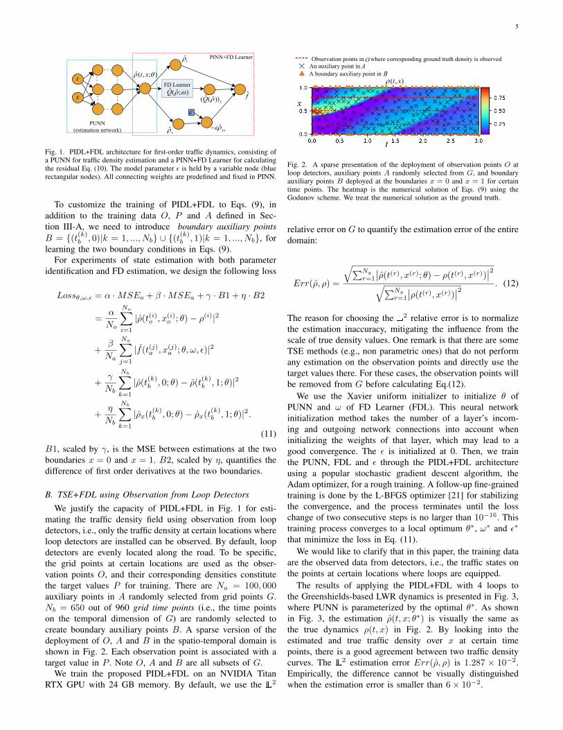
Fig. 1. PIDL+FDL architecture for first-order traffic dynamics, consisting ofa PUNN for traffic density estimation and a PINN+FD Learner for calculatingthe residual Eq. (10). The model parameter ε is held by a variable node (bluerectangular nodes). All connecting weights are predefined and fixed in PINN.

To customize the training of PIDL+FDL to Eqs. (9), inaddition to the training data O, P and A defined in Sec-tion III-A, we need to introduce boundary auxiliary pointsB = {(t(k)b , 0)|k = 1, ..., Nb} ∪ {(t(k)b , 1)|k = 1, ..., Nb}, forlearning the two boundary conditions in Eqs. (9).

For experiments of state estimation with both parameteridentification and FD estimation, we design the following loss

Lossθ,ω,ε = α ·MSEo + β ·MSEa + γ ·B1 + η ·B2

=α

No

No∑i=1

|ρ(t(i)o , x(i)o ; θ)− ρ(i)|2

+β

Na

Na∑j=1

|f(t(j)a , x(j)a ; θ, ω, ε)|2

+γ

Nb

Nb∑k=1

|ρ(t(k)b , 0; θ)− ρ(t(k)b , 1; θ)|2

+η

Nb

Nb∑k=1

|ρx(t(k)b , 0; θ)− ρx(t(k)b , 1; θ)|2.

(11)

B1, scaled by γ, is the MSE between estimations at the twoboundaries x = 0 and x = 1. B2, scaled by η, quantifies thedifference of first order derivatives at the two boundaries.

B. TSE+FDL using Observation from Loop Detectors

We justify the capacity of PIDL+FDL in Fig. 1 for esti-mating the traffic density field using observation from loopdetectors, i.e., only the traffic density at certain locations whereloop detectors are installed can be observed. By default, loopdetectors are evenly located along the road. To be specific,the grid points at certain locations are used as the obser-vation points O, and their corresponding densities constitutethe target values P for training. There are Na = 100, 000auxiliary points in A randomly selected from grid points G.Nb = 650 out of 960 grid time points (i.e., the time pointson the temporal dimension of G) are randomly selected tocreate boundary auxiliary points B. A sparse version of thedeployment of O, A and B in the spatio-temporal domain isshown in Fig. 2. Each observation point is associated with atarget value in P . Note O, A and B are all subsets of G.

We train the proposed PIDL+FDL on an NVIDIA TitanRTX GPU with 24 GB memory. By default, we use the L2

t

x

( , )t x

Observation points in

An auxiliary point in

A boundary auxiliary point in

OA

B

where corresponding ground truth density is observed

Fig. 2. A sparse presentation of the deployment of observation points O atloop detectors, auxiliary points A randomly selected from G, and boundaryauxiliary points B deployed at the boundaries x = 0 and x = 1 for certaintime points. The heatmap is the numerical solution of Eqs. (9) using theGodunov scheme. We treat the numerical solution as the ground truth.

relative error on G to quantify the estimation error of the entiredomain:

Err(ρ, ρ) =

√∑Ng

r=1

∣∣ρ(t(r), x(r); θ)− ρ(t(r), x(r))∣∣2√∑Ng

r=1

∣∣ρ(t(r), x(r))∣∣2 . (12)

The reason for choosing the L2 relative error is to normalizethe estimation inaccuracy, mitigating the influence from thescale of true density values. One remark is that there are someTSE methods (e.g., non parametric ones) that do not performany estimation on the observation points and directly use thetarget values there. For these cases, the observation points willbe removed from G before calculating Eq.(12).

We use the Xavier uniform initializer to initialize θ ofPUNN and ω of FD Learner (FDL). This neural networkinitialization method takes the number of a layer’s incom-ing and outgoing network connections into account wheninitializing the weights of that layer, which may lead to agood convergence. The ε is initialized at 0. Then, we trainthe PUNN, FDL and ε through the PIDL+FDL architectureusing a popular stochastic gradient descent algorithm, theAdam optimizer, for a rough training. A follow-up fine-grainedtraining is done by the L-BFGS optimizer [21] for stabilizingthe convergence, and the process terminates until the losschange of two consecutive steps is no larger than 10−16. Thistraining process converges to a local optimum θ∗, ω∗ and ε∗

that minimize the loss in Eq. (11).We would like to clarify that in this paper, the training data

are the observed data from detectors, i.e., the traffic states onthe points at certain locations where loops are equipped.

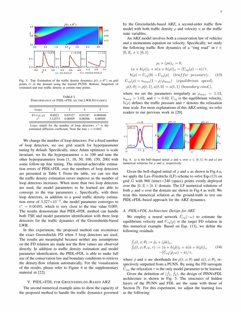
The results of applying the PIDL+FDL with 4 loops tothe Greenshields-based LWR dynamics is presented in Fig. 3,where PUNN is parameterized by the optimal θ∗. As shownin Fig. 3, the estimation ρ(t, x; θ∗) is visually the same asthe true dynamics ρ(t, x) in Fig. 2. By looking into theestimated and true traffic density over x at certain timepoints, there is a good agreement between two traffic densitycurves. The L2 estimation error Err(ρ, ρ) is 1.287 × 10−2.Empirically, the difference cannot be visually distinguishedwhen the estimation error is smaller than 6× 10−2.

6

0.078t 0.234t 1.0t

x

t

*ˆ ( , ; )t x

x true density estimated density

Fig. 3. Top: Estimation of the traffic density dynamics ρ(t, x; θ∗) on gridpoints G in the domain using the trained PUNN. Bottom: Snapshots ofestimated and true traffic density at certain time points.

TABLE IPERFORMANCE OF PIDL+FDL ON THE LWR DYNAMICS

loops 2 3 4 5

Err(ρ, ρ) 0.6021 0.03327 0.01287 0.004646ε∗ 3.12573 0.00495 0.00506 0.00509

loops stands for the number of loop detectors. ε∗ is theestimated diffusion coefficient. Note the true ε = 0.005.

We change the number of loop detectors. For a fixed numberof loop detectors, we use grid search for hyperparametertuning by default. Specifically, since Adam optimizer is scaleinvariant, we fix the hyperparameter α to 100 and tune theother hyperparameters from [1, 10, 50, 100, 150, 200] withsome follow-up fine tuning. The minimal-achievable estima-tion errors of PIDL+FDL over the numbers of loop detectorsare presented in Table I. From the table, we can see thatthe traffic density estimation errors improve as the number ofloop detectors increases. When more than two loop detectorsare used, the model parameters to be learned are able toconverge to the true parameters ε. Specifically, with threeloop detectors, in addition to a good traffic density estima-tion error of 3.327×10−2, the model parameter converges toε∗ = 0.00495, which is very close to the true value 0.005.The results demonstrate that PIDL+FDL method can handleboth TSE and model parameter identification with three loopdetectors for the traffic dynamics of the Greenshields-basedLWR.

In this experiment, the proposed method can reconstructthe exact Greenshields FD when 5 loop detectors are used.The results are meaningful because neither any assumptionson the FD relation are made nor the flow values are observeddirectly. In addition to traffic density estimation and modelparameter identification, the PIDL+FDL is able to make fulluse of the conservation law and boundary conditions to retrievethe density-flow relation automatically. For the visualizationof the results, please refer to Figure 4 in the supplementarymaterial in [22].

V. PIDL+FDL FOR GREENSHIELDS-BASED ARZ

The second numerical example aims to show the capacity ofthe proposed method to handle the traffic dynamics governed

by the Greenshields-based ARZ, a second-order traffic flowmodel with both traffic density ρ and velocity u as the trafficstate variables.

An ARZ model involves both a conservation law of vehiclesand a momentum equation on velocity. Specifically, we studythe following traffic flow dynamics of a “ring road” in t ∈[0, 3], x ∈ [0, 1]:

ρt + (ρu)x = 0,

(u+ h(ρ))t + u(u+ h(ρ))x = (Ueq(ρ)− u)/τ,h(ρ) = Ueq(0)− Ueq(ρ) (traffic pressure),

Ueq(ρ) = umax(1− ρ/ρmax) (equilibrium speed),

ρ(t, 0) = ρ(t, 1), u(t, 0) = u(t, 1) (boundary cond.),

(13)

where we set the parameters irregularly as ρmax = 1.13,umax = 1.02, and τ = 0.02. Ueq is the equilibrium velocity,h(ρ) defines the traffic pressure and τ denotes the relaxationtime scale. For more explanations of this ARZ setting, we referreaders to our previous work in [20].

00.5 10

0.5

1

0.25

0.5

0.75

0.4

0.6

0.8

1

31.5 31.50x

0t

x

(0, )x

(0, )u x

t t

( , )t x ( , )u t x

a) b) c)

1

Fig. 4. a) is the bell-shaped initial ρ and u over x ∈ [0, 1]; b) and c) arenumerical solutions for ρ and u, respectively.

Given the bell-shaped initial of ρ and u as shown in Fig.4.a,we apply the Lax–Friedrichs (LF) scheme to solve Eqs.(13) ongrid G with 960 (time)×240 (space) points evenly deployedover the [0, 3]× [0, 1] domain. The LF numerical solutions ofboth ρ and u over the domain are shown in Fig.4 as well. Wetreat this numerical solution as the ground-truth to test ourPIDL+FDL-based approach for the ARZ dynamics.

A. PIDL+FDL Architecture Design for ARZ

We employ a neural network Ueq(·;ω) to estimate theequilibrium velocity and Ueq(ρ) is the target FD relation inthis numerical example. Based on Eqs. (13), we define thefollowing residuals

f1(t, x; θ) := ρt + (ρu)x,

f2(t, x; θ, ω, τ) := (u+ h(ρ))t + u(u+ h(ρ))x−(Ueq(ρ;ω)− u)/τ,

(14)

where ρ and u are shorthands for ρ(t, x; θ) and u(t, x; θ), re-spectively outputted from a PUNN. By using the FD surrogateUeq , the relaxation τ is the only model parameter to be learned.

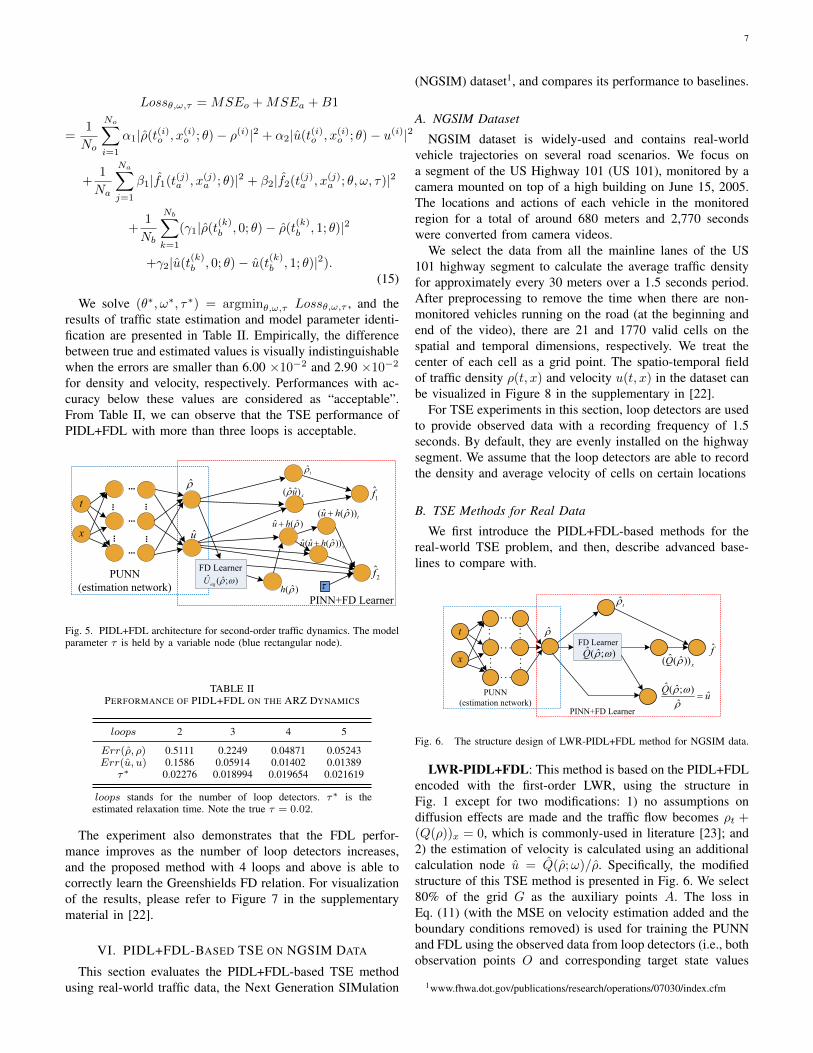
Given the definition of (f1, f2), the design of PINN+FDLarchitecture is shown in Fig. 5. The structures of hiddenlayers of the PUNN and FDL are the same with those ofSection IV. For this experiment, we adjust the learning lossas the following:

7

Lossθ,ω,τ =MSEo +MSEa +B1

=1

No

No∑i=1

α1|ρ(t(i)o , x(i)o ; θ)− ρ(i)|2 + α2|u(t(i)o , x(i)o ; θ)− u(i)|2

+1

Na

Na∑j=1

β1|f1(t(j)a , x(j)a ; θ)|2 + β2|f2(t(j)a , x(j)a ; θ, ω, τ)|2

+1

Nb

Nb∑k=1

(γ1|ρ(t(k)b , 0; θ)− ρ(t(k)b , 1; θ)|2

+γ2|u(t(k)b , 0; θ)− u(t(k)b , 1; θ)|2).(15)

We solve (θ∗, ω∗, τ∗) = argminθ,ω,τ Lossθ,ω,τ , and theresults of traffic state estimation and model parameter identi-fication are presented in Table II. Empirically, the differencebetween true and estimated values is visually indistinguishablewhen the errors are smaller than 6.00 ×10−2 and 2.90 ×10−2

for density and velocity, respectively. Performances with ac-curacy below these values are considered as “acceptable”.From Table II, we can observe that the TSE performance ofPIDL+FDL with more than three loops is acceptable.

...

...

......

......x

t

...

PINN+FD Learner

PUNN

(estimation network)

u

ˆt

ˆ ˆ( )xu1f

ˆ( )h

ˆˆ ( )u h

ˆˆ( ( ))tu h

ˆˆ ˆ( ( ))xu u h

2f

FD Learnerˆ ˆ( ; )eqU

Fig. 5. PIDL+FDL architecture for second-order traffic dynamics. The modelparameter τ is held by a variable node (blue rectangular node).

TABLE IIPERFORMANCE OF PIDL+FDL ON THE ARZ DYNAMICS

loops 2 3 4 5

Err(ρ, ρ) 0.5111 0.2249 0.04871 0.05243Err(u, u) 0.1586 0.05914 0.01402 0.01389

τ∗ 0.02276 0.018994 0.019654 0.021619

loops stands for the number of loop detectors. τ∗ is theestimated relaxation time. Note the true τ = 0.02.

The experiment also demonstrates that the FDL perfor-mance improves as the number of loop detectors increases,and the proposed method with 4 loops and above is able tocorrectly learn the Greenshields FD relation. For visualizationof the results, please refer to Figure 7 in the supplementarymaterial in [22].

VI. PIDL+FDL-BASED TSE ON NGSIM DATA

This section evaluates the PIDL+FDL-based TSE methodusing real-world traffic data, the Next Generation SIMulation

(NGSIM) dataset1, and compares its performance to baselines.

A. NGSIM Dataset

NGSIM dataset is widely-used and contains real-worldvehicle trajectories on several road scenarios. We focus ona segment of the US Highway 101 (US 101), monitored by acamera mounted on top of a high building on June 15, 2005.The locations and actions of each vehicle in the monitoredregion for a total of around 680 meters and 2,770 secondswere converted from camera videos.

We select the data from all the mainline lanes of the US101 highway segment to calculate the average traffic densityfor approximately every 30 meters over a 1.5 seconds period.After preprocessing to remove the time when there are non-monitored vehicles running on the road (at the beginning andend of the video), there are 21 and 1770 valid cells on thespatial and temporal dimensions, respectively. We treat thecenter of each cell as a grid point. The spatio-temporal fieldof traffic density ρ(t, x) and velocity u(t, x) in the dataset canbe visualized in Figure 8 in the supplementary in [22].

For TSE experiments in this section, loop detectors are usedto provide observed data with a recording frequency of 1.5seconds. By default, they are evenly installed on the highwaysegment. We assume that the loop detectors are able to recordthe density and average velocity of cells on certain locations

B. TSE Methods for Real Data

We first introduce the PIDL+FDL-based methods for thereal-world TSE problem, and then, describe advanced base-lines to compare with.

...

...

...

...

...

...

x

t

...

ˆt

f

PUNN

(estimation network)

ˆ ˆ( ; )ˆ

ˆ

Qu

FD Learner

PINN+FD Learner

ˆ ˆ( ; )Q ˆ ˆ( ( ))xQ

Fig. 6. The structure design of LWR-PIDL+FDL method for NGSIM data.

LWR-PIDL+FDL: This method is based on the PIDL+FDLencoded with the first-order LWR, using the structure inFig. 1 except for two modifications: 1) no assumptions ondiffusion effects are made and the traffic flow becomes ρt +(Q(ρ))x = 0, which is commonly-used in literature [23]; and2) the estimation of velocity is calculated using an additionalcalculation node u = Q(ρ;ω)/ρ. Specifically, the modifiedstructure of this TSE method is presented in Fig. 6. We select80% of the grid G as the auxiliary points A. The loss inEq. (11) (with the MSE on velocity estimation added and theboundary conditions removed) is used for training the PUNNand FDL using the observed data from loop detectors (i.e., bothobservation points O and corresponding target state values

1www.fhwa.dot.gov/publications/research/operations/07030/index.cfm

8

P ). After tuning the hyperparameters with grid search, wepresent the minimal-achievable estimation errors. The samefor other baselines by default. Because the real data could benoisy, leading to abnormal learned FD curves, the reshapingregularization term in Eq. (8) is applied.

ARZ-PIDL+FDL: This method is based on the PIDL+FDLencoded with the second-order ARZ, using the structure inFig. 5. The Eq. (15) (with boundary conditions removed) isapplied as the loss function. Other experimental setups are thesame with those of the LWR-PIDL+FDL method.

Two-Dimensional Data Interpolation (Interp2): The two-dimensional linear interpolation method is used as a baseline,which interpolates the traffic states using the neighboringobserved data in a linear manner.

Adaptive Smoothing (AS) Method: This method estimatesthe traffic state of a cell using the sum of all the observeddata weighted by some smoothing kernel filters. We implementa generalized AS method proposed in [10] with parameterssuggested in [24].

Long Short Term Memory (LSTM) based Method: Thisbaseline method employs the LSTM architecture, which iscustomized from the LSTM-based TSE proposed by [11]. Thismodel can be applied to our problem by leveraging the spatialdependency, i.e., to use the information of previous cells toestimate the traffic density and velocity of the next cell alongthe spatial dimension.

Other baselines include the Pure Neural Network (NN) andthe Extended Kalman Filter (EKF) as well as the advancedPIDL-based TSE methods: LWR-based PIDL (LWR-PIDL)and ARZ-based PIDL (ARZ-PIDL). For more descriptionsregarding these four baselines, we refer the readers to theauthors’ previous work in [20].

C. Results and Discussion

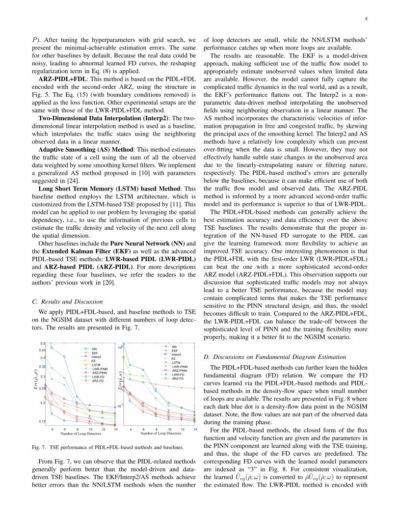
We apply PIDL+FDL-based, and baseline methods to TSEon the NGSIM dataset with different numbers of loop detec-tors. The results are presented in Fig. 7.

4 6 8 10 12 14

0.15

0.2

0.25

0.3

0.35

0.4

0.45

0.5

NN

EKF

AS

interp2

LSTM

LWR-PINN

ARZ-PINN

LWR-FD

ARZ-FD

4 6 8 10 12 14

10-1

100

ˆ(

,)

Erruu

ˆ(

,)

Err

Number of Loop DetectorsNumber of Loop Detectors

NN

EKF

AS

interp2

LSTM

LWR-PINN

ARZ-PINN

LWR-FD

ARZ-FD

Fig. 7. TSE performance of PIDL+FDL-based methods and baselines.

From Fig. 7, we can observe that the PIDL-related methodsgenerally perform better than the model-driven and data-driven TSE baselines. The EKF/Interp2/AS methods achievebetter errors than the NN/LSTM methods when the number

of loop detectors are small, while the NN/LSTM methods’performance catches up when more loops are available.

The results are reasonable. The EKF is a model-drivenapproach, making sufficient use of the traffic flow model toappropriately estimate unobserved values when limited dataare available. However, the model cannot fully capture thecomplicated traffic dynamics in the real world, and as a result,the EKF’s performance flattens out. The Interp2 is a non-parametric data-driven method interpolating the unobservedfields using neighboring observation in a linear manner. TheAS method incorporates the characteristic velocities of infor-mation propagation in free and congested traffic, by skewingthe principal axes of the smoothing kernel. The Interp2 and ASmethods have a relatively low complexity which can preventover-fitting when the data is small. However, they may noteffectively handle subtle state changes in the unobserved areadue to the linearly-extrapolating nature or filtering nature,respectively. The PIDL-based method’s errors are generallybelow the baselines, because it can make efficient use of boththe traffic flow model and observed data. The ARZ-PIDLmethod is informed by a more advanced second-order trafficmodel and its performance is superior to that of LWR-PIDL.

The PIDL+FDL-based methods can generally achieve thebest estimation accuracy and data efficiency over the aboveTSE baselines. The results demonstrate that the proper in-tegration of the NN-based FD surrogate to the PIDL cangive the learning framework more flexibility to achieve animproved TSE accuracy. One interesting phenomenon is thatthe PIDL+FDL with the first-order LWR (LWR-PIDL+FDL)can beat the one with a more sophisticated second-orderARZ model (ARZ-PIDL+FDL). This observation supports ourdiscussion that sophisticated traffic models may not alwayslead to a better TSE performance, because the model maycontain complicated terms that makes the TSE performancesensitive to the PINN structural design, and thus, the modelbecomes difficult to train. Compared to the ARZ-PIDL+FDL,the LWR-PIDL+FDL can balance the trade-off between thesophisticated level of PINN and the training flexibility moreproperly, making it a better fit to the NGSIM scenario.

D. Discussions on Fundamental Diagram Estimation

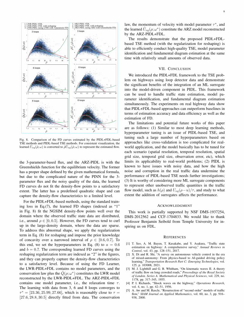
The PIDL+FDL-based methods can further learn the hiddenfundamental diagram (FD) relation. We compare the FDcurves learned via the PIDL+FDL-based methods and PIDL-based methods in the density-flow space when small numberof loops are available. The results are presented in Fig. 8 whereeach dark blue dot is a density-flow data point in the NGSIMdataset. Note, the flow values are not part of the observed dataduring the training phase.

For the PIDL-based methods, the closed form of the fluxfunction and velocity function are given and the parameters inthe PINN component are learned along with the TSE training,and thus, the shape of the FD curves are predefined. Thecorresponding FD curves with the learned model parametersare indexed as “3” in Fig. 8. For consistent visualization,the learned Ueq(ρ;ω) is converted to ρUeq(ρ;ω) to representthe estimated flow. The LWR-PIDL method is encoded with

9

1

23

ˆˆ

(;

)Q

ˆˆ

ˆ(

;)

eqU

1

23

ˆˆ

(;

)Q

ˆˆ

(;

)Q

1. LWR-PIDL+FDL2. LWR-PIDL+FDL with reshaping3. LWR-PIDL (using LWR with 3-parameter FD)

1. ARZ-PIDL+FDL2. ARZ-PIDL+FDL with reshaping3. ARZ-PIDL (using ARZ with Greenshields FD)

12

3

32

1

2

2

1

3

3

ˆˆ

ˆ(

;)

eqU

ˆˆ

ˆ(

;)

eqU

3 loops

6 loops

8 loops

3 loops

6 loops

8 loops

1

Fig. 8. Comparison of the FD curves estimated by the PIDL+FDL-basedTSE methods and PIDL-based TSE methods. For consistent visualization, thelearned Ueq(ρ;ω) is converted to ρUeq(ρ;ω) to represent the estimated flow.

the 3-parameter-based flux, and the ARZ-PIDL is with theGreenshields function for the equilibrium velocity. The formerhas a proper shape defined by the given mathematical formula,but due to the complicated nature of the PINN for the 3-parameter flux and the noisy quality of the data, the learnedFD curves do not fit the density-flow points to a satisfactoryextent. The latter has a predefined quadratic shape and cancapture the density-flow characteristics to a limited level.

For the PIDL+FDL-based methods, using the standard train-ing loss in Eq.(7), the learned FD shapes (indexed as “1”in Fig. 8) fit the NGSIM density-flow points well over thedomain where the observed traffic state data are distributed,i.e., around ρ ∈ [0, 0.5]. However, the FD curves tend to curlup in the large-density domain, where the data are sparse.To address this abnormal shape, we apply the regularizationterm in Eq. (8) for reshaping and impose the prior knowledgeof concavity over a narrowed interval of ρ ∈ [0.6, 0.7]. Tothis end, we set the hyperparameters in Eq. (8) to a = 0.6and b = 0.7. The corresponding learned FD curves using thereshaping regularization term are indexed as “2” in the figures,and they can properly capture the density-flow characteristicsto a satisfactory level. Because of using the FD Learner,the LWR-PIDL+FDL contains no model parameters, and theconservation law plus the Q(ρ;ω∗) constitutes the LWR modelreconstructed by the LWR-PIDL+FDL. The ARZ-PIDL+FDLcontains one model parameter, i.e., the relaxation time τ .The learning with data from 3, 6 and 8 loops converges toτ∗ = [23.36, 25.99, 27.66], which is reasonably close to τ =[27.6, 28.8, 30.5] directly fitted from data. The conservation

law, the momentum of velocity with model parameter τ∗, andthe learned Ueq(ρ;ω∗) constitute the ARZ model reconstructedby the ARZ-PIDL+FDL.

The results demonstrate that the proposed PIDL+FDL-based TSE method (with the regularization for reshaping) isable to efficiently conduct high-quality TSE, model parameteridentification and fundamental diagram estimation at the sametime with relatively small amounts of observed data.

VII. CONCLUSION

We introduced the PIDL+FDL framework to the TSE prob-lem on highways using loop detector data and demonstratethe significant benefits of the integration of an ML surrogateinto the model-driven component in PIDL. This frameworkcan be used to handle traffic state estimation, model pa-rameter identification, and fundamental diagram estimationsimultaneously. The experiments on real highway data showthat PIDL+FDL-based approaches can outperform baselines interms of estimation accuracy and data efficiency as well as theestimation of FD.

The limitations and potential future works of this paperare as follows: (1) Similar to most deep learning methods,hyperparameter tuning is an issue of PIDL-based TSE, andtuning such a large number of hyperparameters based onapproaches like cross-validation is too complicated for real-world application, and the model basically has to be tuned foreach scenario (spatial resolution, temporal resolution, spatialgrid size, temporal grid size, observation error, etc), whichlimits its applicability to real-world problems; (2) PIDL isknown to have issues with noisy data, and how the highnoise and corruption in the real traffic data undermine theperformance of PIDL-based TSE needs further investigations;(3) It is worthy of considering more ML surrogate componentsto represent other unobserved traffic quantities in the trafficflow model, such as h(ρ) and Ueq(ρ−u)/τ , and study to whatextent the addition of surrogates affects the performance.

ACKNOWLEDGMENT

This work is partially supported by NSF DMS-1937254,DMS-2012562 and CCF-1704833. We would like to thankProfessor Benjamin Seibold from Temple University for in-spiring us on FDL.

REFERENCES

[1] T. Seo, A. M. Bayen, T. Kusakabe, and Y. Asakura, “Traffic stateestimation on highway: A comprehensive survey,” Annual Reviews inControl, vol. 43, pp. 128–151, 2017.

[2] X. Di and R. Shi, “A survey on autonomous vehicle control in the eraof mixed-autonomy: From physics-based to AI-guided driving policylearning,” Transportation Research Part C: Emerging Technologies, vol.125, p. 103008, 2021.

[3] M. J. Lighthill and G. B. Whitham, “On kinematic waves II. A theoryof traffic flow on long crowded roads,” Proceedings of the Royal Societyof London. Series A. Mathematical and Physical Sciences, vol. 229, no.1178, pp. 317–345, 1955.

[4] P. I. Richards, “Shock waves on the highway,” Operations Research,vol. 4, no. 1, pp. 42–51, 1956.

[5] A. Aw and M. Rascle, “Resurrection of “second order” models of trafficflow,” SIAM Journal on Applied Mathematics, vol. 60, no. 3, pp. 916–938, 2000.

10

[6] H. M. Zhang, “A non-equilibrium traffic model devoid of gas-likebehavior,” Transportation Research Part B: Methodological, vol. 36,no. 3, pp. 275–290, 2002.

[7] Y. Wang, M. Papageorgiou, and A. Messmer, “Real-time freeway trafficstate estimation based on extended Kalman filter: Adaptive capabilitiesand real data testing,” Transportation Research Part A: Policy andPractice, vol. 42, no. 10, pp. 1340–1358, 2008.

[8] X. Di, H. X. Liu, and G. A. Davis, “Hybrid extended Kalman filteringapproach for traffic density estimation along signalized arterials: Use ofglobal positioning system data,” Transportation Research Record, vol.2188, no. 1, pp. 165–173, 2010.

[9] L. Mihaylova and R. Boel, “A particle filter for freeway traffic estima-tion,” in 43rd IEEE Conference on Decision and Control (CDC), Nassau,Bahamas, 2004, pp. 2106–2111.

[10] M. Treiber, A. Kesting, and R. E. Wilson, “Reconstructing the trafficstate by fusion of heterogeneous data,” Computer-Aided Civil andInfrastructure Engineering, vol. 26, no. 6, pp. 408–419, 2011.

[11] W. Li, J. Hu, Z. Zhang, and Y. Zhang, “A novel traffic flow dataimputation method for traffic state identification and prediction based onspatio-temporal transportation big data,” in Proceedings of InternationalConference of Transportation Professionals (CICTP), Shanghai, China,2017, pp. 79–88.

[12] Z. Zheng, Y. Yang, J. Liu, H.-N. Dai, and Y. Zhang, “Deep and embed-ded learning approach for traffic flow prediction in urban informatics,”IEEE Transactions on Intelligent Transportation Systems, vol. 20, no. 10,pp. 3927–3939, 2019.

[13] Y. Yuan, Z. Zhang, X. T. Yang, and S. Zhe, “Macroscopic traffic flowmodeling with physics regularized gaussian process: A new insightinto machine learning applications in transportation,” TransportationResearch Part B: Methodological, vol. 146, pp. 88–110, Feb. 2021.

[14] M. Raissi and G. E. Karniadakis, “Hidden physics models: Machinelearning of nonlinear partial differential equations,” Journal of Compu-tational Physics, vol. 357, pp. 125–141, Mar. 2018.

[15] Z. Mo, R. Shi, and X. Di, “A physics-informed deep learning paradigmfor car-following models,” Transportation Research Part C: EmergingTechnologies, vol. 130, p. 103240, 2021.

[16] J. Huang and S. Agarwal, “Physics informed deep learning for trafficstate estimation,” in IEEE 23rd International Conference on IntelligentTransportation Systems (ITSC), Sept. 20-23, 2020, pp. 3487–3492.

[17] M. Barreau, J. Liu, and K. H. Johanssoni, “Learning-based state recon-struction for a scalar hyperbolic PDE under noisy lagrangian sensing,”in arXiv preprint arXiv:2011.09871, Nov. 2020.

[18] J. Liu, M. Barreau, M. Cicic, and K. H. Johanssoni, “Learning-basedtraffic state reconstruction using probe vehicles,” in arXiv preprintarXiv:2011.05031, Nov. 2020.

[19] M. Barreau, M. Aguiar, J. Liu, and K. H. Johansson, “Physics-informedlearning for identification and state reconstruction of traffic density,” inarXiv preprint arXiv:2103.13852, Mar. 2021.

[20] R. Shi, Z. Mo, and X. Di, “Physics-informed deep learning for trafficstate estimation: A hybrid paradigm informed by second-order trafficmodels,” Proceedings of the AAAI Conference on Artificial Intelligence,vol. 35, no. 1, pp. 540–547, May 2021.

[21] R. H. Byrd, P. Lu, J. Nocedal, and C. Zhu, “A limited memory algo-rithm for bound constrained optimization,” SIAM Journal on ScientificComputing, vol. 16, no. 5, pp. 1190–1208, 1995.

[22] R. Shi, Z. Mo, K. Huang, X. Di, and Q. Du, “A physics-informed deeplearning paradigm for traffic state estimation and fundamental diagramdiscovery,” in arXiv preprint arXiv:2101.06580, Jun. 2021.

[23] S. Fan and B. Seibold, “Data-fitted first-order traffic models and theirsecond-order generalizations: Comparison by trajectory and sensor data,”Transportation Research Record, vol. 2391, no. 1, pp. 32–43, 2013.

[24] X. Wang, Y. Wu, D. Zhuang, and L. Sun, “Low-rank hankel tensor com-pletion for traffic speed estimation,” arXiv preprint arXiv:2105.11335,2021.