Embed Size (px)
Citation preview
Geophys. J. R . astr. SOC. (1985) 80, 1-34
A perturbation theory for Love waves in anelastic media
G. Madja* Division of Applied Mathematics, Brown ~nivers i ty , Providence, Rhode Island 02912, USA
R. C. Y. Chin and F. E. Followill LawrenceLivermoreNational Laboratory, PO Box 808, Livermore, California 94550, USA
Received 1984 June 5 ; in original form 1983 November 16
Summary. We give a systematic formulation and a rigorous justification of a perturbation technique for the computation of the eigenvalues and eigen- functions of Love waves (and toroidal oscillations by an appropriate change for variables) in an anelastic medium with a constitutive law modelling geophysical media of current interest such as the Kelvin-Voigt Solid, the Maxwell Solid, the Standard Linear Solid, and the Standard Linear Solid with a continuous spectrum of relaxation times. We develop expressions relating the eigenvalues of eigenfunctions for Love waves in a continuously varying vertically stratified anelastic half-space to the corresponding elastic eigen- values and eigenfunctions. Analytically, our correspondence principle has the form of a regular perturbation expansion in terms of a parameter E for both the eigenvalues and eigenfunctions. The identification of E is motivated by the dissipativity principle of viscoelasticity theory. Moreover, we show that our correspondence principle applies respectively only in the high and low frequency range for the Maxwell and Kelvin-Voigt Solids. Outside of the applicable range of frequencies, our correspondence principle yields no useful information. For the family of Standard Linear Solids it is uniformly applic- able for all non-zero frequencies.
We also derive an explicit formula to estimate the radius of convergence of our perturbation expansions. This estimate of the radius of convergence for each eigenvalue and eigenfunction is functionally defined by the consti- tutive model for the anelastic medium. The estimate is frequency dependent and depends on the separation distance between the eigenvalue and the remainder of the spectrum of the corresponding elastic problem.
1 Introduction
For the Fourier transformed anelastic problems, the Lam6 parameters X and p are complex- valued functions. Consequently, the governing equations are non-self-adjoint and have
*Consultant to the Lawrence Livermore National Laboratory. 1
2 mathematical properties differing from the corresponding equations in the elastic case. There are two ways to compute the eigenvalues and eigenfunctions of these non-self-adjoint anelastic problems. One way is to solve the complex boundary value problems directly (Yuen & Peltier 1982). Another way is to establish a correspondence principle between the elastic and the anelastic eigenvalue problems with perturbation techniques. In geophysics, the perturbation approach has been chiefly adopted. In particular, see Anderson & Archambeau (1964), Liu & Archambeau (1975, 1976). (In the mechanics literature, see, for example, Fisher & Leitman 1966.)
Despite numerous articles in the literature, a complete and systematic theoretical treat- ment of the underlying perturbation procedures has not appeared. The analysis must include the identification of an appropriate anelastic perturbation parameter, a systematic procedure to generate all terms in the perturbation series for the eigenvalues and eigenfunctions, and an estimate for the radius of convergence of these series.
In this paper, we consider the problem of Love waves in a continuously varying vertically stratified anelastic half-space using perturbation methods. We are motivated by a need for a complete and systematic theoretical treatment of the perturbation procedures. Thus, our paper contains new and expository sections for didactic reasons. We give a systematic development of the perturbation theory including the identification of the anelastic perturbation parameter for rheological models of geophysical interest, a systematic proce- dure to generate all terms in the perturbation series for the eigenvalues and eigenfunctions, and an estimate for the radius of convergence of these series. We choose the Love wave problem because of its simple mathematical structure.
Four rheological models of current geophysical interest are considered. They are the Maxwell Solid, the Kelvin-Voigt Solid, the Standard Linear Solid (SLS), and the Standard Linear Solid with a continuous spectrum of relaxation times (SLSCS). For the Maxwell and the Kelvin-Voigt Solids, the anelastic perturbation parameter is the usual specific attenua- tion Q-'. The perturbation expansion is, in either case, not uniformly valid for all frequencies. This is a new observation. For the family of Standard Linear Solids (SLS and SLSCS), a new anelastic perturbation parameter is introduced. The anelastic perturbation parameter is given by the reduced modulus defect (ratio of the modulus defect to the instantaneous modulus) and is motivated by the dissipativity principle for viscoelasticity. In these cases, the use of the usual perturbation parameter QZax leads to an unnecessarily complicated formulation of the perturbation equations. Using our new perturbation para- meter, we obtain a renormalization of the usual perturbation expansion using Qzax. This result is new.
Having identified the appropriate anelastic perturbation parameter, we apply a pertur- bation theory (Kato 1966) for non-self-adjoint linear operators to generate all terms in the perturbation expansions for the eigenvalues and eigenfunctions. The zeroth-order terms in these series are solutions of the corresponding elastic Love wave problem.
We also derive estimates for the radius of convergence of the perturbation expansions for the eigenvalues and eigenfunctions. This estimate of the radius of convergence for each eigenvalue and eigenfunction is functionally defined by the constitutive model for the anelastic medium. The estimate is frequency dependent and depends on the separation distance between the eigenvalue and the remainder of the spectrum of the corresponding elastic problem. This estimate is apparently new in solid earth geophysics. We have included a brief review of a perturbation theory for non-self-adjoint linear operators for didactic reasons.
Detailed information about the spectral properties of the Love wave operator in an elastic medium is required in order to apply the perturbation theory. We have extended the results of Hudson (1962) and Kazi (1976) in order to obtain this information.
G. Majda, R. C. Y. Chin and F. E. Followill
A theory for Love waves 3 Hudson (1962) establishes the existence of Love waves in a piecewise-continuous
vertically stratified elastic layer of finite depth with the lower boundary rigidly fixed. For each non-zero frequency, we establish sufficient conditions under which Love waves exist in a continuously varying vertically stratified elastic half-space. In particular, we show that Love waves necessarily exist for the special case in which the shear wave speed is a mono- tonically increasing function of depth. We obtain the conditions for the existence of Love waves when the shear wave speed is not a monotonic function of depth. A theorem is proved that states the existence, at most, of a finite number of isolated eigenvalues. We also show that no Love waves exist for the frequency o = 0.
Kazi (1976) presents a method to obtain all eigenvalues and eigenfunctions (both proper and improper) for the Love wave problem in a piecewise-continuous vertically stratified elastic half-space. He also determines the location of both the continuous and discrete spectra in the case of a constant elastic layer overlying a constant elastic half-space. We establish the location of the discrete and continuous spectra for the Love wave problem in a continuously varying vertically stratified elastic half-space.
Before going on, we remark that the assumption of a continuously varying stratified elastic half-space is made strictly for mathematical convenience. We conjecture that similar results are obtainable in a piecewise continuously varying stratified anelastic solid.
This paper is organized in the following manner: In Section 2, we derive the Love wave equation in a continuously varying vertically stratified anelastic medium. In Section 3 , we identify an appropriate perturbation parameter. In Section 4, we review the abstract pertur- bation theory. In Section 5, we state the necessary theoretical results about the Love wave equation in an elastic medium which are required by the abstract perturbation theory in Section 4. We present in Section 6 a proof of the convergence of the perturbation series and the estimate for the radius of convergence. Our paper ends with a set of conclusions.
Readers who are interested in the conclusions of our work, but not in the mathematical details should omit reading the second half of Section 4 and Lemmas 6.1 and 6.2 in Section 6 .
2 The anelastic Love wave equation
The equations governing the infinitesimal displacement of a material medium in the absence of pre-stress and body forces are given in, for example, Burridge (1976) or Aki & Richards (1980). In Cartesian coordinates, the equations for the conservation of linear momentum is given by
a2u
at2 p(x ) -= v - u.
Equation (2.1) must be satisfied for all points x contained in i2 and for times t 2 0 where
C2 denotes a volume,
x = (x, y, 2) = (XI, x2, x3),
u(x, t ) = [uI(x, r ) , u2(x , r), u3(x , t)lT denotes the infinitesimal displacement. (Superscript T denotes the transpose of a vector.)
p ( x ) denotes the equilibrium density. u(x, t ) denotes the stress tensor.
4 G. MaIda, R. C. Y. Chin and F. E. Followill
The stress-strain constitutive relationship for an anelastic medium is derived in Christensen (1971), Leitman & Fisher (1973), or Pipkin (1972). It is given by
is the classical infinitesimal strain tensor.
Gijkl(x, t ) has the representation We will restrict our discussion to isotropic media. In this case (Christensen 1971),
Gjjkz(x, t ) = 7 3 { G z ( ~ , t ) - G I (X, t ) ) 6ij6kl' % G I ( x , t)(&ikajZ + 6iZbjk) (2.4)
where G l ( x , t ) is called the shear relaxation function, G z ( x , t ) is called the longitudinal relaxation function, and hj j is the Kronecker symbol. The relaxation functions Gi, i = 1 , 2, are represented by
Gi(t) = Gi(0 ) + IOt Gl(7)dT i = 1 , 2 , (2-5)
where the real constants G i ( 0 ) are called the instantaneous moduli. They are related to the elastic response of the medium. If G,(O) = 0, i = 1 , 2 , then the medium has no instantaneous elastic response. If
Gi(-) = lim G,(t)
exist, then Gi(m) are called the equilibrium moduli. The momentum equation (2.1) and the constitutive relation (2.2) form a complete
system of equations when supplemented with appropriate initial and boundary conditions (Aki & Richards 1980).
Next, we derive the equation for Love waves in a continuously varying vertically stratified anelastic half-space. Let
i = 1 , 2 , t-+ -
5 2 = { ( x , z ) : - m < x < m , z 2 O } ,
G i ( x , t ) = Gi(z ,
G z ( x , t ) = Gz(z. t ) ,
P ( X > = P ( Z ) .
u ( x , z , t) . Remark: These conditons imply that u(x , t )= u(x, z , t), ( ( x , t ) = g(x, z, t ) and u(x, t ) =
Assume that the displacement u ( x , z , t ) in (2.1) has the form
u(x , 2 , t ) = (0, V(X, z, t ) , oIT. (2.6)
A theory for Love waves 5
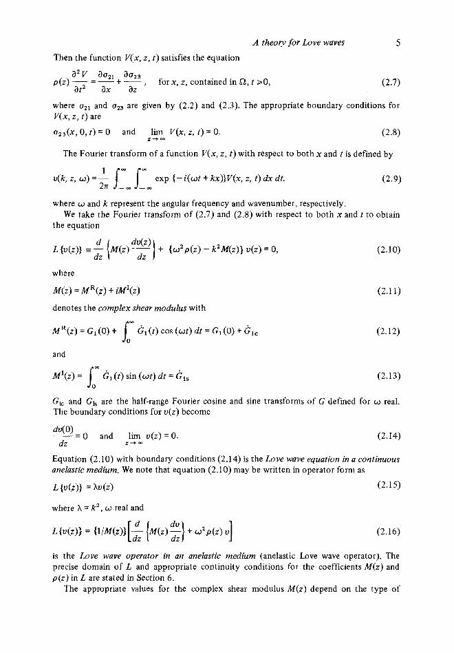
Then the function V(x, z, t ) satisfies the equation
azv aozl aaZ3 at2 ax az
(2.7) p(z) - = - + - , for x, z, contained in 52, t >O,
where uZ1 and (523 are given by (2.2) and (2.3). The appropriate boundary conditions for V(x, z, t) are
uZ3(x, 0, t ) = 0 and lim V(x, z, t ) = 0. 2'-
The Fourier transform of a function V(x, z, t ) with respect to both x and t is defined by
1 - -
27l - m u(k, z, w) = - 1 1- exp { - i ( o t + kx)}V(x, z, t ) dx dt.
where w and k represent the angular frequency and wavenumber, respectively.
the equation We take the Fourier transform of (2.7) and (2.8) with respect to both x and t to obtain
d
dz 1 dz 1 L {u(z)} = - M ( z ) du(z) - + {w2p(z) - k2M(z)} u(z) = 0, (2.10)
where
M(z) = M R ( z ) i- iM'(z) (2.1 1)
denotes the complex shear modulus with
MR(z) = G1 (0) +
and
M'(z) = /om G l ( t ) sin ( a t ) d t = GIs
G1 ( t ) cos ( a t ) dt = Gl(0) i- &Ic l (2.12)
(2.13)
GI, and Gk are the half-range Fourier cosine and sine transforms of G defined for u real. The boundary conditions for u(z) become
-- d'(o)- 0 and lim u(z) = 0. dz z+-
(2.14)
Equation (2.10) with boundary conditions (2.14) is the Love wave equation in a continuous anelastic medium. We note that equation (2.10) may be written in operator form as
L { u ( 2 ) ) = xu (2 ) (2.15)
where h = k2, w real and
(2.16)
is the Love wave operator in an anelastic medium (anelastic Love wave operator). The precise domain of L and appropriate continuity conditions for the coefficients M ( z ) and p(z) in L are stated in Section 6 .
The appropriate values for the complex shear modulus M ( z ) depend on the type of
6
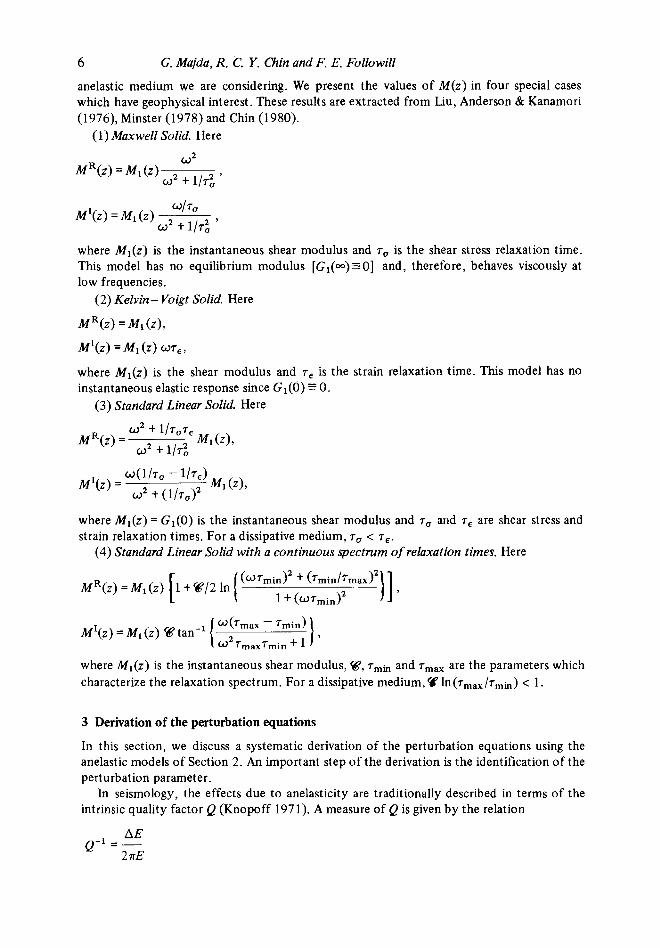
anelastic medium we are considering, We present the values of M ( z ) in four special cases which have geophysical interest. These results are extracted from Liu, Anderson & Kanamori (1976), Minster (1978) and Chin (1980).
G. Majda, R . C. Y . Chin and F. E. Followill
(1) Maxwell Solid. Here
w2 M R ( z ) = M1 ( z )
w2 t 1/r: '
wITu
w2 + 117: ' M'(z) = M1 ( z )
where Ml(z) is the instantaneous shear modulus and T,, is the shear stress relaxation time. This model has no equilibrium modulus [Gl(m)=O] and, therefore, behaves viscously at low frequencies.
(2 ) Kelvin- Voigt Solid. Here
M R ( z ) = M i ( z ) ,
M'(z) = M1 ( z ) wr,,
where M l ( z ) is the shear modulus and T~ is the strain relaxation time. This model has no instantaneous elastic response since G1(0) 0.
( 3 ) Standard Linear Solid. Here
where M l ( z ) = Gl(0) is the instantaneous shear modulus and 7, arid r, are shear stress and strain relaxation times. For a dissipative medium, T,, < 7,.
(4) Standard Linear Solid with a continuous spectrum of relaxation times. Here
where M l ( z ) is the instantaneous shear modulus, ", ~~h and r,,, are the parameters which characterize the relaxation spectrum. For a dissipative medium,% ln (Tmax / rm~) < 1.
3 Derivation of the perturbation equations
In this section, we discuss a systematic derivation of the perturbation equations using the anelastic models of Section 2 . An important step of the derivation is the identification of the perturbation parameter.
In seismology, the effects due to anelasticity are traditionally described in terms of the intrinsic quality factor Q (Knopoff 1971). A measure of Q is given by the relation
A theory for Love waves 7
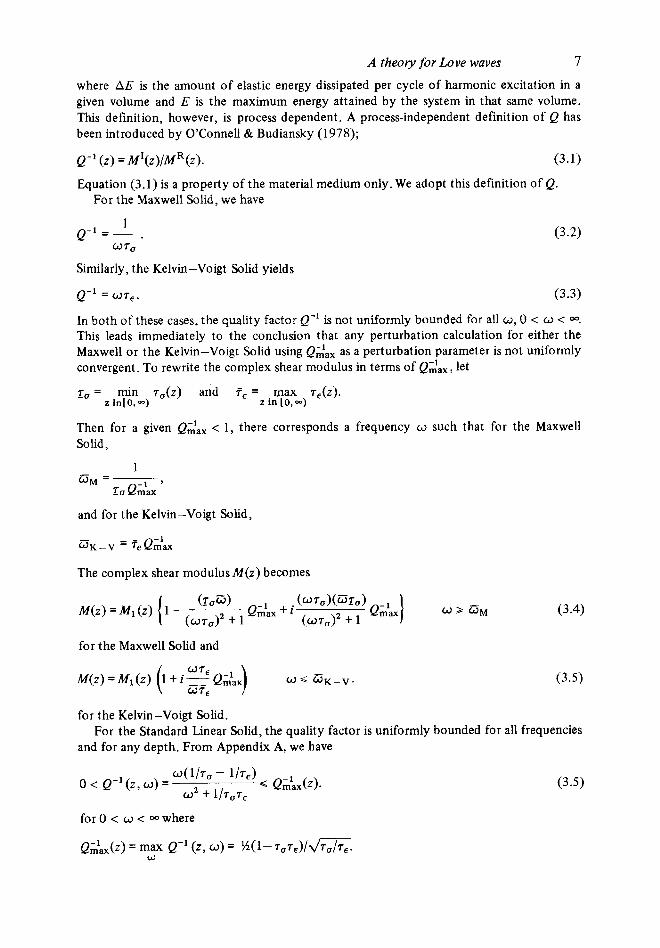
where AE is the amount of elastic energy dissipated per cycle of harmonic excitation in a given volume and E is the maximum energy attained by the system in that same volume. This definition, however, is process dependent. A process-independent definition of Q has been introduced by O'Connell & Budiansky (1978);
Q-' ( z ) = M'(z)/MR(z). (3.1)
Equation (3.1) is a property of the material medium only. We adopt this definition of Q. For the Maxwell Solid, we have
1
a 7,
Q-1 =-
Similarly, the Kelvin-Voigt Solid yields
Q-' = wr,. (3.3)
In both of these cases, the quality factor Q-' is not uniformly bounded for all w, 0 < w < m.
This leads immediately to the conclusion that any perturbation calculation for either the Maxwell or the Kelvin-Voigt Solid using QZax as a perturbation parameter is not uniformly convergent. To rewrite the complex shear modulus in terms of QZax, let
lo = min r,(z) and T6 = rnax r&). z inl0.m) z in [o, -)
Then for a given Q2ax < 1 , there corresponds a frequency w such that for the Maxwell Solid,
a M = p y
and for the Kelvin-Voigt Solid,
1
~u Q$ax
a~ - v = Tc Qi'ax
The complex shear modulus M ( z ) becomes
for the Maxwell Solid and
for the Kelvin-Voigt Solid.
and for any depth. From Appendix A, we have For the Standard Linear Solid, the quality factor is uniformly bounded for all frequencies
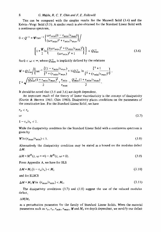
8 This can be compared with the simpler results for the Maxwell Solid (3.4) and the
Kelvin-Voigt Solid (3.5). A similar result is also obtained for the Standard Linear Solid with a continuous spectrum,
G. Majda, R. C. Y. Chin and F. E. Followill
) ] Q Q;ix + F ~ ~ [ (WTmin)' + (Tmin/Tmax)'
(UTmin)' + 1
for 0 < o < 00, where QZax is implicitly defined by the relations
It should be noted that (3.5 and 3.6) are depth dependent. An important result of the theory of linear viscoelasticity is the concept of dissipativity
(Gurtin & Herrera 1965; Chin 1980). Dissipativity places conditions on the parameters of the constitutive law. For the Standard Linear Solid, we have
While the dissipativity condition for the Standard Linear Solid with a continuous spectrum is given by
@In (Tmax/Tmin) < 1. (3.8)
Alternatively the dissipativity condition may be stated as a bound on the modulus defect A M
AM = MR(z, w = m) - MR(z, w = 0). (3 -9)
From Appendix A, we have for SLS
AM = M1 ( 1 - T,/T,) < M I
and for SLSCS
( 3 . 1 0 )
AM = Mi @ In (Tmax/Tmin) < M I . (3.1 1)
The dissipativity conditions (3.7) and (3.8) suggest the use of the reduced modulus defect,
A W M l
as a perturbation parameter for the family of Standard Linear Solids. When the material parameters such as T,, 7€, ~ , h , T ~ ~ ~ , %?and M1 are depth dependent, we modify our defini-
A theoly for Love waves 9 tion of the perturbation parameter E so that
(3.12)
Associated with this choice of E , there is a depth2 for which the stated maximum is attained. The complex shear modulus of the family of Standard Linear Solids may be rewritten as
~ ( z , u) = M ~ ( z , W ) + iM'(z, W )
Since,
MR(z, 0) Q MR(z, W ) Q MR(z, -) =Mi,
therefore,
MR(z, W ) -Mi(z) MI M1 (Z) (z)z=iG
for all o and z .
Koenig relation (Leitman & Fisher 1973), we have Morever, since M'(z, W ) is the conjugate function ofMR(z, w ) by virtue of the Kramers-
This clearly demonstrates the appropriateness of (3.12) as a perturbation parameter. Let us point out the disadvantages of using the traditional value
as the perturbation parameter. Here, the expansion of the shear modulus is an infinite series in L, and it is valid only for < 1 . For SLS, we have from Appendix A,
For Q&x < 1, we have
AM
M1 - _ - 2Qi:x (1 - Q;ix + %(QA~x)2 . . .} .
A similar expansion may be obtained for SLSCS. The expansion parameter in this case is
Q&x In (7max/Tmin).
The expression (3.13) is nice in that it contains only first-order terms. This should be compared with the use of QZax as an expansion parameter. That procedure gives an infinite series of operators. Note that (3.13) suggests that the first-order corrections are frequency dependent, It is also expected that the spectrum of the anelastic Love wave operator con- verges uniformly to its associated elastic spectra as E + 0. This will be proved in Section 6.
10 Having properly identified the anelastic perturbation parameter E , we develop the pertur-
bation equations in what follows. Note that the complex shear modulus for the Maxwell Solid (3.4), the Kelvin-Voigt Solid (3.5), and the family of Standard Linear Solids (3.13) may be written in the generic form
M(z) = M l ( z ) [ 1 + e { M R ( z ) + iM'(z ) } ] . (3.14)
Substituting (3.14) into the anelastic Love wave equation, we obtain the following expan- sion for the anelastic Love wave operator:
G. Majda, R. C. Y. Chin and F. E. Followill
m
L = 1 E"L(") n = O
where
M(z) = M R ( ~ ) + iM'(z)
(3.15)
We remark that the higher order perturbation operators L(") n > 1 have complex-valued coefficients which are continuous and bounded on [0, -). The elastic Love wave operator L('), on the other hand, has strictly real, continuous and bounded coefficients. This completes the derivation of the perturbation equations.
4 Formulation of a general perturbation theory
In this section we review the formulation and rigorous verification of a general perturbation theory (Kato 1966) for the computation of eigenvalues and eigenfunctions of linear operators. The purpose is entirely pedagogical and for the sake of completeness. The reader should consult Kato's text for any undefined terminology.
H denotes a Hilbert space. ( u , v ) denotes the innerproduct of any two elements u , u in H. [I u I I = ( (u , u ))1'2 denotes the norm of any element u in H.
i.e. 11 Un-u 11 tends to zero as n tends to infinity.
Not at ion :
Let U,, , n = 1, 2 . . ., and u be elements in H , then Un + u denotes convergence in norm,
For any linear operator L with its domain and range contained in H ,
I/ Lu II I1 L il = sup - sup II Lu II I I U I I + o II u I1 II u I I = 1 u in H u in H
denotes the norm of the linear operator L .
A theory for Love waves 11 For any set S and any element B contained in S, denote the complement of S with
respect to B by SIB. We are now prepared to formulate the perturbation theory. Let T( j ) , j = 0, 1, 2 .. -, be
given linear operators. Consider the linear operator T(E) depending on a complex parameter e denoted by
cu
T ( € ) = c T ( W (4.1) j = O
with domain D (a subset of H). The eigenvalue problem for T(e) consists of finding all scalar functions A(€) and non-trivial functions u(e) contained in D which satisfy
T(E) u(e) =A(€) u(e). (4.2)
The scalar functions A(€) are called the eigenvalues of T(e) and the functions u(e) are called the corresponding eigenfunctions.
We make the following assumptions about the operator T<O):
Assumption 4.1: The operator T(O) with domain D is self-adjoint with respect to the inner product ( -, . >.
Assumption 4.2: For each eigenvalue A(') of T(O), the null space (Kato 1966, p. 142) of the operator ( T ( O ) - A ( O ) ) has dimension one.
Assumption 4.3: For each eigenvalue A(') of T(O), the operator (T( ' ) -A(O)) with domain D and mapping D into Hsatisfies the Fredholm alternative (Stakgold 1967, p. 172).
Remark 4.1: Let A(') denote any eigenvalue of T(O) and let do) denote a corresponding eigenfunction. Assumptions 4.1-4.3 imply that for any f i n Hthere exists a solution u in D of the equation
- A(@) u = f
if and only if
(u(O), f ) = 0.
Moreover, the solution is non-unique.
satisfies the conditions in Assumptions 4.1 -4.3.
we assume that A(€) and U ( E ) may be computed with the regularperturbation expansions
Remark 4.2: In Section V we show that the Love wave operator in an elastic medium
We consider operator (4.1) under the condition that E is small (i.e. I e I Q 1). For this case
m
A(€) = c A(")€" n =O
and oc
U ( E ) = 1 u%", n =O
where u (e) satisfies the normalization condition
(4.4)
to eliminate the non-uniqueness of the solution. A simple computation shows that (4.5) may be written as
12 Substitute expansions (4.3) and (4.4) into (4.1) to obtain
G. Majda, R. C. Y. Chin and F. E. Followill
Equating like powers of E in (4.7), we obtain the following hierarchy of equations for the coefficients of expansions (4.3) and (4.4):
(4.8)
(4.9)
(4.10)
and, more generally,
(T(o ) - h(0)) .(n) = f h ( ~ ) ~ ( n - j ) - T( i lu (n - j ) , n = 3 , 4 , . . . . (4.1 1)
is an eigenvalue of the unperturbed operator T(O) and
j = 1 j = 1
Equation (4.8) shows that
By remark 4.1, equation (4.9) has a solution u( l ) if and only if u(O) is a corresponding eigenfunction of T(O). For convenience, we choose (do), do) ) = 1.
(u(o), - T ( ' ) U ( O ) ) = 0.
This implies that
l ( 1 ) = ( T(OU(O), u(o))* (4.12)
The function u(') is determined by solving equation (4.9) subject to the normalization condition (4.6) for j = 1.
In a similar fashion, (4.10) has a solution provided that
(u(o) , h(')u(l) + - ( T q p + T ( 2 ) U ( O ) ) ) = 0.
(4.13)
The function d2) is determined by solving equation (4.8) subject to the normalization condition (4.6) for j = 2.
and &) for j = 0, 1, . . . , n-1 . Then by remark 4.1
Finally, assume that we have determined
(4.14)
The function u(n) is determined by solving equation (4.1 1) subject to the normalization condition
(u("), = 0. (4.15)
The infinite series (4.3) and (4.4) with coefficients determined by equations (4.12)- (4.14) are valid only if they are convergent. We now present general conditions for the operator RE) which can be checked and used to establish that (4.3) and (4.4) are conver-
A theoly for Love waves 13
gent expansions. We also provide an estimate for the radius of convergence of expansions (4.3) and (4.4).
We begin with four definitions. Definition 4.1: Let T and A be linear operators with the same domain space X (but not
necessarily the same range) such that the domain of T is contained in the domain of A. A is relatively bounded with respect to T if there exist constants a, b > 0 such that
for all u contained in the domain of T. The greatest lower bound of all constants b satis- fying (4.16), denoted by bo, is called the relative bound of A with respect to T.
Remark 4.3: The concept of relative boundedness of two operators is an extremely important and useful one. It gives a way of measuring the size of a perturbation even when the perturbation is an unbounded operator.
Definition 4.2: A linear operator T mapping the space X into the space Y is closed if for any sequence of functions { u, } with each u, contained in the domain of T , the condi- tions u, -+ u and Tun -+ y imply that u is contained in the domain of T and Tu = y . The space of closed operators mapping X into Y is denoted by C ( X , Y ) .
Definition 4.3: Let T be an operator in C ( X , Y ) and let y denote a complex number. (i) m e resolvent set of T = {y: ( T - y ) is invertible and (T-y)-' is a bounded operator}.
(ii) The spectrum of T = {r: Either (T -y ) is not invertible or (T -y ) is invertible but
We now introduce a family of operators which includes many differential operators
Definition 4.4: A family of linear operators T(E) contained in C ( X , Y ) and defined for
The resolvent set of Tis denoted by p(T) .
(T-y)-' is not bounded}. The spectrum of Tis denoted by Z ( T ) .
(including the Love wave operator in an anelastic medium).
each E in a domain Do in the complex plane is said to be holomorphic o f type A if
family T(E) is independent of E . )
I
(i) Domain T(E) = domain of T(0) = D for each e contained in Do. (i.e. the domain of the
(ii) T(e)u is holomorphic for every E contained in Do and every u contained in D.
Conditions (i) and (ii) imply that T(E)u = T(')u + eT(l)u + E'T(~)u + . . . for each u in D, E = 0 belongs to Do, and that this series converges in a disc I e I < r independent of u.
Holomorphic operators of type A will play an essential role in our discussion. Therefore we present a useful criterion which guarantees that a given family of operators belongs to this class.
Theorem 4.1 (criterion for operators of type A )
Let T(') be a closed linear operator mapping X into Y with domain D. Let T("), n = 1, 2 , . . . , be linear operators mapping X into Y with domains containing D, and let there be constants a, b, c 2 0 such that
)I T(")u I 1 4 c" - ' (a 1 1 u 11 + b ( I T(')u 1 1 ) (4.17)
for every u contained in D and n = 1, 2 , . . . . Then the series T(E) given by (4.1) defines an operator with domain D for 1 E 1 < l/c. If 1 e 1 < (b + c)-', T(E) is a closed operator and forms a holomorphic family of type A .
We are now prepared to state the main results of the perturbation theory regarding the convergence of expansions (4.3) and (4.4) for the eigenvalues and eigenfunctions of (4.1).
14
Theorem 4.2 (convergence for an isolated eigenvalue)
Consider the infinite series of operators (4.1) with domain D. Assume that
G. Majda, R. C. Y. Chin and F. E. Followill
(i) T ( E ) forms a holomorphic family of type A . (ii) is an isolated eigenvalue of T(O) with corresponding eigenfunction do). Let r be any closed curve in the complex plane which lies in p(T(O)) . the resolvent set of
T(O), and encloses the eigenvalue Xco) and no other eigenvalue of 7"'). (r exists because A(') is isolated.) Then at least for all complex E satisfying
I E I Q r min [ (b + c)- ' , min ( a II R ( y , T(O)) ( I + b (I T(')R(y, T(O)) I1 + c ) - ' ]
where a, b and c are the constants which appear in Theorem 4.1 and
R(y , T(O)) = (T(O) - y)-', (4.19)
there exists an eigenvalue X ( E ) and an eigenfunction u(e) to T(E) which can be computed by using convergent regular perturbation expansions (4.3) and (4.4). These expansions converge at least for all complex E satisfying I E I =G r .
(4.18) y o n r
Theorem 4.3 (convergence for a finite number of isolated eigenvalues)
Consider the infinite series of operators (4.1) with domain D. Assume that
(i) T(e ) forms a holomorphic family of type A . (ii) T(O) has a finite number of isolated eigenvalum denoted by A:?), j = 1, . . . , N , with
corresponding eigenfunctions denoted by u y ) , j = 1, . . . , N .
Let ri, j = 1, . . . , N , be any closed curve in the complex plane which lies in p(T(O)) and encloses the eigenvalue Xf" and no other eigenvalue of T(O). (ri exists because A;?) is isolated.)
Set
ri = min { ( b + c)- ' , min [a II R ( y , T(O)] II + b II T(')R [y, T(O)] II + c ] - ' }
where a, b, c and R(y, T(O)) are defined in Theorem 4.2, and
R" = min {r i } . (4.2 1) i
Then at least for all complex E satisfying 1 € 1 G i, and each value of j = 1, . . ., N , there exists an eigenvalue Xi(€) and eigenfunction u ~ ( E ) of T(E) which can be computed by using the regular perturbation expansions (4.3) and (4.4) (with h(0) = A:?) and u(0) = u y ) ) . For each value of j = 1 , . . . , N , the expansions for hi(€) and u ~ ( E ) converge at least for all complex E satisfying I E I Q ri.
As a final comment, we note that the lower bound for the radius of convergence of the perturbation expansions which is defined by (4.20) is easily estimated in the case when T(O) is a self-adjoint operator. If y lies in the resolvent set of T(O) and T(O) is self-adjoint, then
(4.20) y o n rj
(4.22)
A theory for Love waves 15
and
(4.23)
These results follow from the spectral mapping theorem (Kato 1966, p. 177). Therefore, if T(') is a self-adjoint operator, hi is an isolated eigenvalue of T('), and ri is a closed curve which lies in p(TCo)) and separates X i from the remainder of C(T(')), then equation (4.20) becomes
r j=min [ (b+c) - ' , min { a max (lh--yi)- ' y o n r j hinZ(T(*))
(4.24)
The theory discussed in this section is complicated. Therefore, we summarize the steps which must be done in order to apply it.
Suppose that we are given the operator T ( E ) defined by (4.1) and we wish to compute the eigenvalues and eigenfunctions of (4.1) with the regular perturbation expansions (4.3) and (4.4) where the coefficients in these expansions are determined by equations (4.12)-(4.15). Let the eigenvalues of T(0) be denoted by Xy), j = 1 , 2 , . . . , N (N could be infinity). In order to determine the values of E for which we can guarantee that expansions (4.3) and (4.4) are valid (convergent) for a particular eigenvalue hp(e) and eigenfunction up(€) of T(E) , we must do the following steps:
(1) Verify that T ( E ) forms a holomorphic family of type A . This may be doneby applying Theorem 4.1. The coefficients a and b which appear on (4.16) may be computed by apply- ing Lemma C.2 which appears in Appendix C.
(2) Compute the eigenvalue hp) of the unperturbed operator T(O). (3) Compute (estimate) the distance between $1 and Z(T('))/hV). (This distance is
called the separ:tion distance of the eigenvalue X?).) This is usually done by computing all remaining eigenvalues of T(') (or estimating where they are) and also locating all points in the continuous spectrum of T(') (or estimating where they are), and then computing (estimating) the distance between A$') and C(T('))/Xf').
Remarks 4.4: (a) If hf') is an isolated eigenvalue of T('), then the separation distance of hf)) is positive. (b) If the separation distance of X f ) ) is zero, then the regular perturbation expansions (4.3) and (4.4) for A t ) and up(€) need not be valid.
(4) Find a closed curve rp which encloses the eigenvalue X t ) and separates if) from Z(T( ' ) ) /A t ) . This curve will usually be determined after we have computed the separation distance of the eigenvalue A t ) .
Remark 4.5: If X f ) ) is an isolated eigenvalue of T('), then a curve rp with the above properties exists.
(5) Find the complex values of E for which the expansions (4.3) and (4.4) are valid by applying equation (4.1 8) if T(') is not self-adjoint and (4.24) if T(O) is self-adjoint.
5 Spectral results for the Love wave operator in an elastic medium
In this section we collect some results regarding the Love wave operator in an elastic medium. We need these results in order to apply Kato's theory to the Love wave operator in an anelastic medium. For completeness, we have included the proofs of the theorems of this section in Appendix B.
16 G. Majda, R. C. Y. Chin and F. E. Followill
Notation: C denotes the set of all complex-valued functions defined for 0 Q z < -. C[O, =) denotes the set of all functions contained in C which are continuous for
For any positive integer j , Ci[O, m) denotes the set of all functions contained in Cwhich
The Love wave operator in an elastic medium is given by
O < z < = .
are j times continuously differentiable on 0 Q z < 00.
where 0 Q w < = is a given constant and Ml(z), p (z ) are real-valued, positive functions. We assume that
M1 ( 2 ) is contained in C2 [0, =)
p ( z ) is contained in C[O, m),
(5.2)
(5.3)
and there exist positive constants, h, M: and ph so that
M1 ( z ) = M: and p ( z ) = p h for z > h. (5.4)
Remark 5.1: The assumptions imply that positive constants M , , M1, p and p exist so that
Let 6 denote the complex conjugate of any function w in C, MI 4 Ml(z) =G fil and P G p(z) Q p for all 0 Q z < 00.
/I w II = (( w, w p , H = w in C: II w II > 00.
The domain of L(O) is denoted by D. The set D consists of all functions u in Csuch that
(i) u is differentiable and du/dz is absolutely continuous (Royden 1968) on 0 G z Q b
(ii) u and L(O) [u] are contained in H , (iii) du/dz (0) = 0 , (iv) lim u(z) = 0.
The eigenvalue problem associated with Lf') consists of finding all scalars h and non-
for all b < 00,
z - + -
trivial functions u in D so that
L(')[u] = hu. (5.5)
Theorem 5.1 For each frequency 0 Q w < w, the Love wave operator L(O) with domain
Theorem 5.2 For each frequency 0 G w < 00, the Love wave operator L(O) with domain D is self-adjoint with respect to the inner product < ., . ).
A theory for Love waves 17
D has at most a finite number ofisolated eigenvalues (there may be no eigenvalue) which all lie in the interval
and a continuous spectrum which lies in the interval
(- 3. Theorem 5.3
(a) If
then for each frequency 0 < w < 00 the Love wave operator L(O) with domain D has at least one eigenvalue.
(b) If w = 0, then L(O) has no eigenvalue. Theorem 5.4 For each frequency 0 < w < m, let A denote an arbitrary eigenvalue of
(a) The dimension of the null space of the operator (L(') - A ) with domain D is exactly one.
(b) Let u(z) denote the solution of the equation (L(') - A) V = 0 (u(z) is uniquely deter- mined except for an arbitrary multiplicative constant). Then for any function f i n H there exists a solution u in D of the equation (L(') - h)u = f if and only if ( u , f ) = 0. Therefore, the operator (L(') -A) with domain D satisfies the Fredholm alternative.
Remark 5.2: Kazi (1976) determined the location of the eigenvalues and continuous spectrum for the Love wave operator in a medium which consists of a constant elastic layer over a constant elastic half-space. His result agrees with the general result given in Theorem 5.2.
Remark 5.3: The integral condition in Theorem 5.3 is satisfied if the shear wave speed of the elastic medium, given by d { M l ( z ) } / { ~ ( z ) } , is a monotonically increasing function of depth.
L(O). Then:
6 Application of the perturbation theory to the Love wave equation in an anelastic medium
In Section 2 we derived the anelastic Love wave operator L defined by (2.16). We then introduced an appropriate perturbation parameter E and rewrote the operator L in terms of this parameter given by (3.15) and labelled the result L ( e ) . The corresponding elastic Love wave operator, denoted by L(O), is obtained by setting e = O in (3.15). In this section we derive a correspondence principle between the eigenvalue of and L(E) . In particular, we prove that if the perturbation parameter E is sufficiently small, then for each eigenvalue X i and eigenfunction ui of the operator L(O) there exists a corresponding eigenvalue X i ( € ) and eigenfunction ui(e) of L (e) which may be computed by using regular perturbation expansions. We also estimate the radius of convergence of these perturbation expansions.
The Love wave equation in an anelastic medium is derived in Section 2:
L W ) I = W ) (6.1)
18 where h = k 2 ,
G. Majda, R . C. Y. Chin and F. E. Followill
L{L'(z)} = ( l / M ( z ) } - M ( z ) - + 0 2 p ( z ) u [3 3 I is the anelastic Love wave operator, o is a given real constant, p ( z ) is a positive function defined for 0 G z < m, and M ( z ) = M R ( z ) + iM'(z) is a complex-valued function defined for 0 G z < 00 with M R ( z ) positive for 0 Q z < 00. We assume that
M ( z ) is contained in C 2 [0, -),
p(z) is contained in C[O, -),
(6.3)
(6.4)
and there exist positive constants h, p h and a complex constant Mh so that
M ( z ) = M h a n d p ( z ) = p h f o r z > h . (6-5)
The domain of L is given by the set of all complex-valued functions lying in D , the set defined in the beginning of Section 5.
The elastic Love wave equation corresponding to L ( E ) is given by
where
is the corresponding elastic Love wave operator. Remark 6 .1: In this section we will always assume that
Consequently, by Theorems 5.2 and 5.3 we are assured that for each frequency w + 0 the operator L(O) has a finite number of isolated eigenvalues denoted by hy), j = 1, . . . , N , and corresponding eigenfunctions denoted by u y ) , j = 1, . . . , N .
If we rewrite M ( z ) in terms of the appropriate perturbation parameter E as done on (3.14), then equation (6.1) may be written as
m
L(E)[U(f)] = L(O'[u(e)] + c € j L ( j ) [ U ( E ) ] = h(e) U(f) j = 1
where the operators L(' ) , ] = 1 , 2, . . . , are defined by (3.16). For each value of j = 1, . . . , N , let
and
n = l
A theoly for Love waves 19
Substitute (6.8) and (6.9) into (6.7) and equate like powers o f f to obtain the following set of equations relating A?) and uj"), n = 0, 1, . . . ,:
(6.10)
Apply Theorem 5.4 to conclude that for each value of n = 1, 2, . . . , equation (6.10) has a solution u?) if and only if
(6.1 1)
where ( ., .) is the inner product defined in Section 5. Relation (6.1 1) determines A?) uniquely. It is easy to show that u p ) is uniquely deter-
mined if we require that (ui"), up)) = 0. Moreover, (6.1 1) is simplified further by choosing (u(O), u p ) ) = 1 to yield
(6.12)
We now show that (6.8) and (6.9) are convergent perturbation expansions if E is suffi-
Lemma 6.1 Let L("), n = 0, 1, . . . , b e the operators defined by (3.16) and let ciently small.
for any complex valued function #(z), 0 < z < 00. Then
for every u contained in D and n = 1 , . . . , where
and 6 is any positive constant which satisfies 016 II d/dz(lnMl) IIc < 1 . Proof: The operators L ( j ) , j = 0 , 1 , . . . , may be written as
20 G. Majda, R . C. Y. Chin and F. E. Followill
dM du o Z p M u , LWU = - - - ___
dZ dZ Mi
and
L@)U = (-M)" - 'L( ' )u ,
Now apply Lemma (2.2 in Appendix C to complete the proof.
n = 2 , . . . , .
Lemma 6.2. The operator L ( E ) with domain D forms a holomorphic family of type A if
Proof: If I E I < l/Cl, then [ l + EM(Z)]-' may be expanded in terms of a geometric series and L ( E ) has the expansion (6.7). The operator L(O) is self-adjoint and therefore closed (Kato 1966, p. 269), so we may apply Theorem 4.1 to complete the proof.
Theorem 6.1. A correspondence principle for Love waves in anelastic media: convergence of regular perturbation expansions for the eigenvalues and eigenfunctions of the anelastic Love wave operator
Let hp) and Uio), j = 1, . . . , N , denote the eigenvalues and eigenfunctions of the operator
E I < (C, + C3)-' where C1 and C, are the constants defined in the preceding lemma.
Let ri be any closed curve in the complex plane which lies in the resolvent set of and encloses the eigenvalue A?) and no other eigenvalue of L(O). Set
(6.13)
and R =min ri
i where Ci, i = 1 , 2, 3, are defined in Lemma 6.1. Then at least for all E satisfying I E I < R" and all values of j = 1, . . . , N , there exists an eigenvalue X i ( € ) and eigenfunction I+(€) of L ( E ) which may be computed by using the regular perturbation expansions (6.8) and (6.9). For each value of j = 1, . . . , N , the expansions for hi (€ ) and u ~ ( E ) converge at least for all E satis- fying I E I c r;.
Proof If I E I < R" the operator L ( E ) forms a holomorphic family of type A by Lemma 6.2. Furthermore, the operator L(O) is self-adjoint and has a finite number of isolated eigen- values. So an application of Theorem 4.3 completes the proof of the correspondence principle.
Let d; denote the separation distance between h(0) and Z(L(O))/h?) and let Fi denote a circle with centre Xg") and radius di/2. Then (6.13) becomes
-
(6.14)
We conclude that the estimate of the radius of convergence of the regular perturbation expansions (6.8) and (6.9) is a function of the separation distance between A?) and 2(L(o))/h$o). The estimate for the radius of convergence (6.14) also depends upon the values of the constants Ci, i = 1 , 2 , 3 . These constants are frequency dependent and function- ally defined by the constitutive model of the anelastic medium.
For completeness, we list upper bounds for the values of the constants Cj, i = 1, 2 , 3 , for an anelastic medium which is modelled as a Maxwell Solid, a Kelvin-Voigt Solid or a Standard Linear Solid.

A theoly for Love waves
(1) Maxwell Solid
We use (3.4) to determine that for all frequencies w > GM = eU QZax)-’, c1 < 1
21
where 6 is any positive constant satisfying a6 I1 d/dz (In M l ) IIc < 1 .
( 2 ) Kelvin- Voigt Solid
We use (3.5) to determine that for all frequencies w <GK-v = TEQZa,
c1 < 1
where 6 is any positive constant satisfying a6 IJ d/dz (In M I ) Ilc < 1.
( 3 ) Standard Linear Solid
We use (3.13), (A7) and (A8) to determine that for all frequencies 0 < w < 00,
c 1 < 1 ,
where
where 6 is any positive constant satisfying a6 I I d/dz (In M I ) (Ic < 1. Remarks (1) Similar bounds may be obtained for the case of a standard linear solid with a
continuous spectrum of relaxation times. These expressions are lengthy and have been omitted.
(2) It may be possible to improve the estimate for the radius of convergence (6.18) by making a different choice for the curve ri which appears in Theorem 6.1. We refer the reader to Kato’s text for further details.
22
7 Conclusions
We have established a correspondence principle for the eigenvalues and eigenfunctions of Love waves in a continuously varying vertically stratified anelastic half-space. Analytically, our correspondence principle has the form of a regular perturbation expansion in terms of a parameter e for both the eigenvalues and eigenfunctions. The identification of E is moti- vated by the dissipativity principle of linear viscoelasticity theory. For the Maxwell and Kelvin-Voigt Solids, it is the specific attenuation factor Q-'. For the family of Standard Linear Solids, it is the reduced modulus defect. It is easy to show that our perturbation series reduces to the closed-form correspondence principle given by Fisher and Leitman in the particular case of a homogeneous half-space with constant coefficients. Moreover, our correspondence principle applies respectively only in the high and low frequency ranges for the Maxwell and Kelvin-Voigt Solids. Outside the applicable range of frequencies, our correspondence principle yields no further information. Other techniques must be employed to study the Love wave problem in the Maxwell or the Kelvin-Voigt Solids. For the family of Standard Li,near Solids, however, our correspondence principle is uniformly applicable for all frequency ranges.
We also derive an explicit formula to estimate the radius of convergence of our pertur- bation expansions. This estimate of the radius of convergence of our regular perturbation expansions for each anelastic eigenvalue and eigenfunction depends on the separation distance between the eigenvalue and the remainder of the spectrum of the corresponding elastic problem. The radius of convergence for each particular eigenvalue also depends upon the vahes of two constants, a and b , These two c,onstants are frequency dependent and functionally defined by the constitutive model of the anelastic medium.
A conformal mapping of the interior of a circle (an equatorial plane of the earth) on to a semi-infinite strip may be used to transform the coordinates of the toroidal oscillation problem into the coordinates of the Love waves in a vertically stratified half-space. This transform allows us t o handle the toroidal oscillation problem; therefore, we give a rigorous justification of a perturbation technique for both toroidal oscillations and Love waves.
We found it necessary to extend the results of Hudson and Kazi on the associated elastic Love wave boundary value problem to provide theorems in the existence, locations and denumeration of eigenvalues which are the basis for our correspondence principle.
G. Majda, R. C. Y. Chin and F. E. Followill
Acknowledgments
We thank our colleagues G. W. Hedstrom, P. Deift and D. W. Thoe for many helpful discussions. We also thank the referee for carefully going over our manuscript. This work was performed under the auspices of the US Department of Energy by the Lawrence Liver- more National Laboratory under Contract No. W-7405-ENG-48.
References
Aki, K. & Richards, P. G., 1980. Quantitative Seismology, Theory and Methods, two volumes, W. H. Freeman, San Francisco.
Anderson, D. L. & Archambeau, C. B., 1964. The anelasticity of the Earth,J. geophys. Res., 69,2071- 2084.
Burridge, R., 1976. Some mathematical topics in seismology, Lecture Notes, Courant Institute of Mathe- matical Sciences, New York.
Chin, R. C. Y., 1980. Wave propagation in viscoelastic media, in Physicsof the Earth's Interior, pp. 213- 246, Enrico Fermi International School of Physics, Course 78, eds Dziewonski, A. & Boschi, E., North-Holland, Amsterdam.
A theory for Love waves 23
Christensen, R. M., 1971. Theory of Viscoelasticity, an Introduction, Academic Press, New York. Coddington, E. A. & Levinson, N., 1955. Theory of Ordinary Differential Equations, McGraw-Hill,
Fisher, G. M. C. & Leitman, M. J., 1966. A correspondence principle for free vibrations of a viscoelastic
Gurtin, M. E. & Herrera, I., 1965. On dissipation inequalities and linear viscoelasticity, Q. appl. Math.,
Hartman, P., 1964. Ordinary Differential Equations, Wiley, New York. Hudson, J. A., 1962. Love waves in a heterogeneous medium, Geophys. J. R . astr. Soc., 6,131-147. Kato, T., 1966. Perturbation Theory for Linear Operators, Springer-Verlag, New York. Kazi, M. H., 1976. Spectral representation of the Love wave operator, Geophys. J. R. astr. Soc., 47,
Knopoff, L., 1971. Proceedings of the International School of Physics, Enrico Fermi, Academic Press,
Leitman, M. J. & Fisher, G . W. C., 1973. The linear theory of viscoelasticity, in Handbuck der Physik,
Liu, H. P., Anderson, D. L. & Kanamori, H., 1976. Velocity dispersion due to anelasticity; implications
Liu, H. P. & Archambeau, C. B., 1975. The effect of anelasticity on periods of the Earth’s free oscilla-
Liu, H. P. & Archambeau, C. B., 1976. Correction to ‘The effect of anelasticity on period of the Earth’s
Minster, J. B., 1978. Transient and impulse responses of a one-dimensional linearly attenuating medium’-
O’Connell, R. J . & Budiansky, B., 1978. Measures of dissipation in viscoelastic media, Geophys. Res.
Pipkin, A. C. , 1972. Lectures on Viscoelasticity Theory, Springer-Verlag, New York. Reed, M. & Simon, B., 1980. Methods of Modern Mathematical Physics; Vol. IV, Analysis o f Operators,
Royden, H. L., 1968. Realilnalysis, 2nd edn, Macmillan, Toronto, Ontario. Rudin, W., 1974. Realand Complex Analysis, 2nd edn, McGraw-Hill, New York. Stakgold, I., 1967. Boundary Value Problems o f Mathematical Physics, Volume I, Macmillan, New York. Titchmarsh, E. C., 1962. Eigenfunction Expansions Assockted with Second Order Ordinary Differential
Weinberger, H. F., 1974. Variational Methods for Eigenvalue Approximations, Regional Conference Series
Yuen, D. A. & Peltier, W. R., 1982. Normal modes of the viscoelastic earth, Geophys. J. R. astr. Soc., 69,
New York.
solid, Trans. ASME J. appl. Mech., 924-926.
23,235-245,
225-249.
New York.
Mechanics o f Solids III, VIa/3, ed Truesdell, Springer-Verlag, Berlin.
for mantle composition, Geophys. J. R. astr. Soc., 47,41-58.
tions (toroidal modes), Geophys. J. R. astr. Soc., 43,795-814.
free oscillations (toroidal modes)’, Geophys. J. R. astr. Soc., 47, 1-7.
I. Analytical results, Geophys. J. R. astr. Soc., 52,479-501.
Lett., 5 , 5 .
Academic Press, New York.
Equations, Part I, 2nd edn, Oxford University Press, London.
in Applied Mathematics No. 15, SIAM, Philadelphia.
495-526.
Appendix A: calculation of QZax
In this appendix, we develop the expressions for QZax for a Standard Linear Solid (SLS) and a Standard Linear Solid with a Continuous Spectrum (SLSCS).
Standard Linear Solid (SLS)
The real and imaginary parts of the shear modulus are given by
and
24 Here re(z) > T,,(z) > 0 by the dissipativity condition (Chin 1980). Hence, the quality factor Q-' as a function of depth z is
G. Majda, R, C. Y. Chin and F. E. Followill
At any depthz, Q-' attains a maximum Qzax(z) with respect to o at w = w. Here,
1
is(z) = d m ) and
Treating (A5) as a quadratic in @ = ~T, , (Z) /T~(Z) , we have
oz + 2 Q;ix @ - 1 = 0.
The solution is
Note that the modulus defect AM is given by
A M = M R ( z , w = ~ ) -MR(z,w=O)=MI(z)(l -T , /T€) .
Using (A5) and (A6), we obtain
we have
m
= 2Ml(z)QA1ax 1 An<QA'ax>". n = O
Using the modulus defect AM to rewrite M R and MI, we obtain
1 - T,/T, MR(z) = MI (z) (1 - W2 T t ( Z ) + 1
AM = M1 ( z ) -
w2T:(z) + 1
A theory for Love waves 25 and
Since
we have
I M ~ - M ~ ( Z ) I < A M
and
M'(z) < AM/2.
Moreover, AM is a bounded and monotonically increasing function of Qzax.
Standard Linear Solid with a Continuous Spectrum (SLSCS)
Similar results may be derived for the Standard Linear Solid with a continuous spectrum. However, the analysis is complicated by the additional parameters contained in the SLSCS model,
The real and imaginary parts of the shear modulus and, hence, the quality factor are given by
and
Q-' (z) =M1(z)/MR(z).
Here, the SLSCS model contains the parameters '$7, ~~h and T ~ ~ ~ . The dissipativity condi- tion (Chin 1980) is given by
O < Y In ( ~ m a x / ~ m i n ) < 1 for all z .
At any depth z , it can be proved that Q-' has a unique maximum with respect to w. The maximum, QZax is attained at w = 0 given by the solution of
(TminG)' + Q A x ( 1 + Tmin/Tmax) TrninB - ~ m i n / ~ r n a x = 0 (A 14)
and
(Al 5 ) tan-' [Tmina/ ((Tminz)2 + Tmin/rmax)(l - rmin/Tmax)l
1 + '$7/2 In {(TminB)' + (Tmin/Tmax>2) /{(TminQ12 + 1) QiiX =
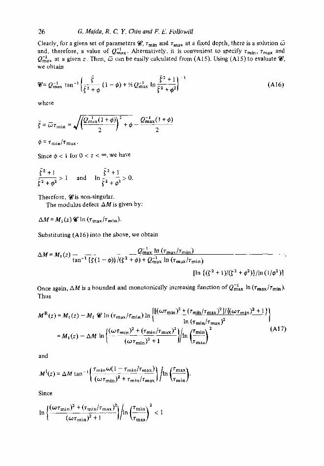
26 Clearly, for a given set of parameters ‘if?, ~,h and T , ~ ~ ~ at a fixed depth, there is a solution W and, therefore, a value of QZax. Alternatively, it is convenient t o specify rmh, rma, and QZax at a given z . Then, W can be easily calculated from (Al.5). Using (A1.5) to evaluate Q, we obtain
G. Majda, R . C. Y, Chin and F. E. Followill
where
Therefore, %is non-singular. The modulus defect AM is given by:
Substituting (A16) into the above, we obtain
AM = M1 ( z ) QiL In ( ~ m a x / ~ r n i n )
tan-’ $11 /(t’ + 4) + Q A x In (Tmax/Tmin)
[In {(t2 + Mt2 + 42))/ln(1/d)2)1
Once again, AM is a bounded and monotonically increasing function of Qzax In ( T ~ ~ / T , ~ ) .
Thus
and
Since
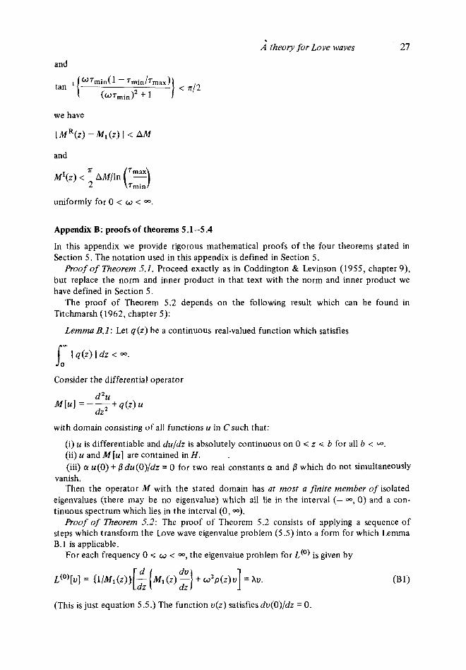
A theory for Love waves 27
and
we have
I MR(z> -MI ( z ) I < AM
and n
M'(z) < - AM/ln 2
uniformly for 0 < w < m.
Appendix B: proofs of theorems 5.1-5.4
In this appendix we provide rigorous mathematical proofs of the four theorems stated in Section 5. The notation used in this appendix is defined in Section 5.
Proof of Theorem 5.1. Proceed exactly as in Coddington & Levinson (1955, chapter 9), but replace the norm and inner product in that text with the norm and inner product we have defined in Section 5.
The proof of Theorem 5.2 depends on the following result which can be found in Titchmarsh (1962, chapter 5):
Lemma B.1: Let q ( z ) be a continuous real-valued function which satisfies
IOa I q(z ) I dz < -.
Consider the differential operator
d 2 u
dz2 M [ u ] =---+q(z)u
with domain consisting of all functions u in Csuch that:
(i) u is differentiable and du/dz is absolutely continuous on 0 G z Q b for all b < a. (ii) u and M [u] are contained in H . (iii) a! u(0) + /3 &(O)/dz = 0 for two real constants a and /3 which do not simultaneously
vanish. Then the operator M with the stated domain has ar most a finite member of isolated
eigenvalues (there may be no eigenvalue) which all lie in the interval (- 00, 0) and a con- tinuous spectrum which lies in the interval (0 , -).
Proof of Theorem 5.2: The proof of Theorem 5.2 consists of applying a sequence of steps which transform the Love wave eigenvalue problem (5.5) into a form for which Lemma B.l is applicable.
For each frequency 0 g w < m, the eigenvalue problem for L(O) is given by
(This is just equation 5.5.) The function u(z) satisfies du(O)/dz = 0.
28 G. Majda, R. C. Y. Chin and F. E. Followill
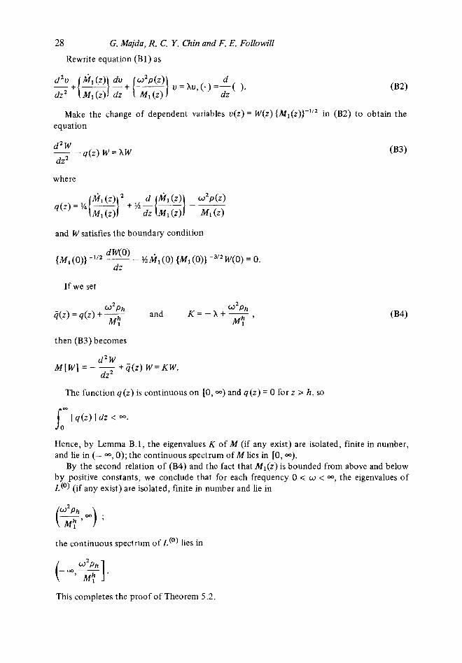
Rewrite equation ( B l ) as
dz
Make the change of dependent variables u(z) = W(z) {M1(z))-”’ in (B2) to obtain the equation
- - q ( z ) W = A W d 2 W
dz2
where
and W satisfies the boundary condition
If we set
then (B3) becomes
d 2 W
dz2 M [ W ] = - - t i j ( 2 ) W = K W .
The function q(z) is continuous on [0, -) and q(z ) = 0 for z > h, SO
IOm I 4 ( z ) I dz < -.
Hence, by Lemma B . l , the eigenvalues K of M (if any exist) are isolated, finite in number, and lie in (- -, 0); the continuous spectrum of M lies in [0, -).
By the second relation of (B4) and the fact that M l ( z ) is bounded from above and below by positive constants, we conclude that for each frequency 0 Q u < -, the eigenvalues of L(O) (if any exist) are isolated, finite in number and lie in
the continuous spectrum of L(O) lies in
This completes the proof of Theorem 5.2.
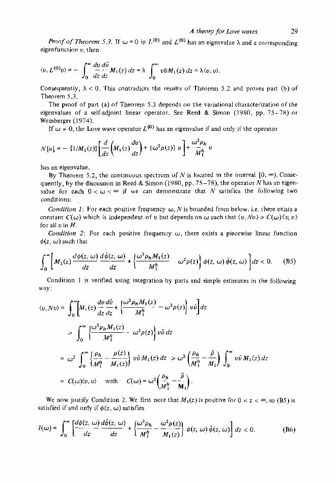
A theoly for Love waves 29 Proof of Theorem 5.3. If w = 0 in L(O) and L(O) has an eigenvalue h and a corresponding
eigenfunction u , then
Consequently, X < 0. This contradicts the results of Theorem 5.2 and proves part (b) of Theorem 5.3.
The proof of part (a) of Theorem 5.3 depends on the variational characterization of the eigenvalues of a self-adjoint linear operator. See Reed & Sinion (1980, pp. 75-78) or Weinberger (1974).
If w # 0, the Love wave operator L(O) has an eigenvalue if and only if the operator
has an eigenvalue. By Theorem 5.2, the continuous spectrum of N is located in the interval [0, -). Conse-
quently, by the discussion in Reed Rr Simon (1980, pp. 75-78), the operator N has 2n eigen- value for each 0 < w < if we can demonstrate that N satisfies the following two conditions:
Condition I : For each positive frequency w , N is bounded from below, i.e. there exists a constant C(w) which is independent of u but depends on w such that ( u , N u ) B C(w)(u, u ) for all u in H.
Condition 2: For each positive frequency 0, there exists a piecewise linear function $(z , w) such that
Condition 1 is verified using integration by parts and simple estimates in the following way:
= C(w)(u, u ) with C(w) = a'(* - &) M:
We now justify Condition 2 . We first note that M l ( z ) is positive for 0 i z < -, so (B5) is satisfied if and only if $(z, w ) satisfies
30 G. Majda, R. C. Y. Chin and F. E. Followill
For each positive value of w , set
and let S(w) be any constant which satisfies 6(w) > l /IK(w) I . Define @(z, w ) by
1 O Q z G h
1 - (z-h)/b(o) @(z, w) = h < z < h t S(w),
h + 6(w) Q z. L Substitute @(z, w ) into (B6) to obtain
= K(w) + { 6 ( ~ ) } -'. Thus, Z(w) is negative by the choice of 6(w).
pp. 230-231), for each frequency w in 0 < w < 00, the operator Proof of Theorem 5.4 (part a): By Corollary 1 in Coddington & Levinson (1955,
d du N [ u ] = - Ml(Z)- + W'PU
dz dz is in the limit-point case at 00 (Stakgold 1967, p. 297). Therefore, by Weyl's Theorem (Stakgold 1967, p. 297), for each complex constant h there is at most one non-trivial soh - tion of the equation (L(O) - h)u = 0 which lies in H . In particular, if h is an eigenvalue of L(O), then the dimension of the null space of (L(O) - h) is exactly one.
(Proof of part b): Assume that there exists a function u contained in D which satisfies - h)u = f. The operator (L(O) -h) with domain D is self-adjoint with respect to the
inner product ( ., . ), so we have
( u , f ) = (u , ( d o ) - A) u ) = ( ( J P ) - A) u, u ) = 0.
We now show that for any function f contained in H which satisfies ( u, f > = 0, there exists a solution u in D of the equation
( d o ) - h) u = f. 037)
The coefficients of (L(O) - h) are real-valued, so it suffices to prove this existence theorem in the case when f is real-valued.
Let W(z) be a solution of the equation (I,(') - h)W = 0 which is independent of u(z). By part (a) of this theorem, W(z) cannot be contained in D. The functions u(z) and W ( z ) lie in C2 [0, 00) and
u(z) = C1 exp (- hz)
W ( z ) = C2 exp (hz) t C3 exp(-hz)
for h G z < 00, (B8)
039) for h G z < 00,
where C1, C2 and C3 are constants with C1, C2 # 0 and X f Jw2pl,/M:. Simple calculations show that there exist non-negative constants K1 and K 2 so that
I u(z) I G K1 exp (- hz) for 0 < z < 00, (B 10)
A theory for Love waves 31
diu < K 1 exp(-hz) f o r j = 1 , 2 a n d O ~ z < - , I2 I
1 2 1 G K 2 exp (hz) f o r j = 1 ,2 and 0 G z < -.
I W(z) I G K2 exp(hz) for 0 G z < -, (B 12)
and
d i W (B 13)
(Here, 1 . I denotes absolute value.) For the moment we assume that the forcing function f(z) lies in Cz [0, -) and satisfizs
I f(z) I G p(z) exp ( -hz) for 0 G z < - (B 14)
where p(z) is some polynomial in z. Set
= loZ 4 z ) W ( 5 ) f(t) M1 (U d t + 1 W(z) U ( t ) f(E)Ml(U dC;. 0315)
The function @(z) is determined by the method of variation of constants, (Hartman 1964, pp. 327-328). We will show that @(z) is a solution of equation (B7) which lies in D .
Conditions (BlO), (B12) and (B14) imply that both integrands in (B15) are integrable over their respective ranges. Since both integrands in (B15) lie in C2 [0, w), @(z) is contained in C2 [O, -).
Take the absolute value of both sides of equation (B15) and estimate using the triangle inequality and bounds (BlO), (B12) and (B14) to obtain
Integrate the second integral in (B16) by parts to obtain the inequality
@(z) G d z ) exp (-hz) (B17)
where 4(z) is a polynomial such that degree [q(z)] = degree [p(z)] + 1. Inequality (B17) implies that @(z) lies in H and
lim u(z)=O z -0
We differentiate @(z) to obtain
32 G. Majda, R. C. Y. Chin and F. E. Followill
Equation (B18) implies that
We differentiate both sides of (B18) to obtain
Take the absolute value of both sides of equation (B19) and apply the triangle inequality and results (BlO)-(B13) to obtain
where i ( z ) is some polynomial. Therefore,
lies in H.
This result together with the fact that d@/dz lies in C' [0, m) implies that d@/dz is absolutely continuous.
Straightforward differentiation of @(z) defined by (B15) in the manner used to obtain (B18) and (B19) shows that (L(O) -A ) @ ( z ) = f ( z ) , that is, @(z) is a solution of (B7). Since f(z) lies in H, (L(O) -A) @(z) lies in H a n d the proof of part (b) is complete when the forcing functionf(z) lies in C'(0, m) and satisfies (B14).
The set of all functions f(z) which lie in Cz[O, m) and satisfy (B14) is dense in H , so standard arguments from Lebesgue integration theory (Royden 1968) may be used to show that part (b) holds for any functionf(z) contained in H .
Appendix C: two useful lemmas
In this appendix we derive two useful lemmas which can be used to compute the relative boundedness coefficients a and b which appear in Lemmas 6.1 and 6.2.
Let p ( z ) denote any piecewise-continuous, positive function defined for 0 G z < -which satisfies
p < i (el) where p and ii denote positive constants.
For any two functions u, w contained in C (the set Cis defined in Section 5) set
I I w I I = (w, W Y ,
A theory for Love waves 33
and
H = ( w i n C : 1 1 w I I < -).
A simple calculation using (CI) yields the inequality
for any function w in H . Lemma C.1 If u, duldz and d2u/dzZ are contained in H , then
where 6 < 0 is an arbitrary positive constant. Proof: This result follows immediately from (1.13) of Kato (1966, p. 192) and (C2). LemmaC.2: Let
and
be two differential operators with coefficients which are continuous and bounded on [0, -). Assume that the domains of both S and T consist of functions t i such that u , du/dz and d2u/dz2 are contained in H .
N , = .max 1 qi(z) I , j = O , 1 , 2 ,
mo = min I po(z ) I ,
Let
z.in [ O , - )
zin[O,-)
and
Mi= max I p j ( z ) I , j = 1 , 2 .
If mo > 0 and 6 is any positive number satisfying mo > M16a
then
I I Su I I a I I u I I + b I I Tu I1
z in [ 0,-)
with
No + 016 N 1 b =
mo - 016 M I 1
2
34 and
G. Majda. R. C. Y. Chin and F. E. Followill
a = N 2 + - N , + 2ff ( M 2 + - M ’,” b 6
and
cu=m. The proof of this lemma mimics example 1.10 of chapter IV in Kato (1966).


