A PDE FORMULATION AND NUMERICAL SOLUTION

FOR A BOLL WEEVIL-COTTON CROP MODEL

RICHARD M. FELDMAN and GUY L. Cum&

Biosystems Research Division, Industrial Engineering Department, Texas A & M University, College Station. TX 77843, U.S.A.

(Received August 1982)

Abstract-A system of partial differential equations is developed that describes the population dynamics and interactions of a boll weevil cotton crop system. Emphasis is placed on the mathematical structure needed in capturing the biologically meaningful interactions between the boll weevil and its host (the cotton buds and fruit). A procedure is outlined for the numerical solution of the system and comparisons are made with field data.

1. INTRODUCTION The mathematical description of biological populations began with the simple exponential

growth curve of Malthus[l] at the close of the 18th century. Since that time, much effort has

gone into increasingly realistic and complex mathematics for describing growing populations.

One of the disadvantages of the early work was the assumption of independence between birth

and/or death rates and the age of the organism. In 1959, Von Foerster[2] presented a two

dimensional partial differential equation formulation in which the population was represented

by a density function with both time and age as independent variables.

The utilization and application of the Von Foerster structure for actual field populations

have not kept pace with their theoretical development. Within the agriculture industry,

modeling for pest management necessitates the description of expanding populations. In other

words, transient conditions are of primary interest; equilibrium and stability analysis are not

usually relevant in pest control decisions. It is also necessary to obtain a high degree of

biological realism so that the effect of untried control tactics can be reasonably well predicted.

The additional equations and functions needed for fully describing the biological processes

usually give rise to structures not analyzed in theoretical works.

The purpose of this paper is to develop and numerically approximate the solution of a

system of partial differential equations that accurately describe the dynamic relationship

between the boll weevil (Anthonomus grandis Boheman) and the cotton plant (Gossypium

hirsutum L.). One of the initial uses of the Von Foerster structure for describing field

populations was by Wang et al.[3]. The major modeling emphasis in [3] was on the cotton plant

although a simplified boll weevil model and its interaction was included. A simplified cotton

crop fruiting model is given in Curry et al.[4].

In Section 2, the necessary biological relationships are summarized and the system of

equations describing the boll weevil-cotton crop is given. The particular emphasis of the model

is the crop-insect interactions including such aspects as the fruit size preference effect on

oviposition site selection, the site scarcity effect on total reproduction, and the fruit drying

effect on immature mortality. The biological facts needed for the Von Foerster system are

taken from [5] and [6]. One of the characteristics of the equations will be that the derivative of

an organism’s age with respect to time is not constant. (It is a function of the environomental

temperature.) Some background information regarding the utilization of multiple variables and

nonconstant derivatives in Von Foerster equations can be found in [7].

2. THE MODEL

Both plants and insects are poikilotherms (cold-blooded) and thus their birth and death rates

not only depend upon their age, but also on temeprature. To compensate for this temperature

dependence, the age of the organism is measured on a transformed time scale instead of

+Joint appointment with Industrial Engineering and Agricultural Engineering Departments

393

394 R. M. FELDYAK and G. L. CURRY

according to chronological time. The age on the transformed scale is called “physiological age”

and on this scale developmental times can be considered independent of temperature. This

transformation works as follows: let Tk be a random variable representing developmental time

under the constant temperature k and let r(+) be the mean rate function, i.e.

r(k) = E[lIT,]. (1)

If IL(t) denotes the temperature at chronological time t, then the physiological age at time t of the

organism born at time zero is

I r

a(t) = r(W)) ds. 0

(2)

The standard approach in biological modeling is to let both time and age be measured in the

same units so that da/dt equals 1. This, however, is frequently not possible for multiple species

because of differing developmental rates.

It is easier to develop the equations for the boll weevil using two stages (immature and

adult) instead of a single stage. The developmental rates for the two stages are significantly

different. Furthermore, the immature stage (egg through pupa) is in a protected environment

and is unaffected by pesticide applications; whereas the adults are free moving and would

therefore be exposed to treatments. The adult female lays her complement of eggs inside the

cotton fruiting structures (flower buds and young fruit)-usually one egg per site. At the time of

the second instar molt, a chemical substance is released by the larvae which causes the fruiting

form (bud or young fruit) to be abscised (dropped) from the plant. The term fruit will

henceforth represent the total fruiting structure. Immature mortality is directly related to the

size of the fruit in which the egg is laid since the major cause of mortality in buds is due to the

bud drying out before the immature reaches a critical size (begins pupation). This mortality

factor is much less pronounced in fruit (after bloom cotton bolls) since they are larger and have

slower drying characteristics. However, they are a much less viable food source and the innate

survival averages about l/2 to l/3 of that in large flower buds. The fruit size is directly related

to its physiological age and thus to fully describe the dynamics of the immature weevil it is

necessary to know the age of the fruit in which the egg was oviposited.

The equations describing the number density of the immature boll weevil, N,, for a given

time t 2 0, physiological age of immatures a, L 0, and within a fixed fruit size s 2 0, is

Ndf, 0, s) = WC &NW, 4s)) I‘ W, aY’J,(t, a) da, 0

(3b)

with the following definitions: NI is the number density function for immature weevils; NA is

the number density function for adult weevils; NF is the number density function for the fruit;

rr is the developmental rate function for the immatures; pr is the mortality rate function for the

immatures due to fruit drying; pE is the rate of emergence of immatures into the adult stage; A

is the egg laying rate function for adult weevils in a crop of unlimited ovipositional sites; B is a

birth function for immatures and is a function of the availability of fruit; o is a function relating

fruit size to the fruit’s physiological age; and 8, is the proportion of females in the population.

Equation (3b) includes several different aspects of reproduction. The intrinsic birth rate, A,

gives the egg laying rate for a female weevil not limited by a lack of ovipositional sites (i.e. buds

or young fruit). The determination of h first necessitates obtaining an empirical function

describing the age dependent reproduction rate of the weevil. Namely, the function R is needed

where zyxwvutsrqponmlkjihgfedcbaZYXWVUTSRQPONMLKJIHGFEDCBARfk, a3 is the expected cumulative reproduction in the (adult) age interval [0, aJ under

the constant temperature regime k”C conditioned on the weevil living at least until age az. The

total reproductive potential of an adult who lives to its maximum age at temperature k is given

by R(k) and the density function giving the reproductive profile with respect to age is i(ad

A PDE formulation and numerical solution for a boll weevil-cotton crop model 395

where for each k and al_ z 0,

R(k) = lim R(k, a), (I-

(4)

and

It is indicated in [8] that the reproductive profile, f, can often be assumed independent of

temperature. Thus, the effect of temperature is through the physiological age and the R

function. The intrinsic birth rate can now be defined, for t, az 2 0, by

Act, ar) = B(ICl(t))i(az)rA(9(t)), (6)

where \Cr(t) is the temperature at time t, R and F are defined by equations (4) and (5) and rA is

the developmental rate function for the adult weevils.

As the number of fruit decrease, there is a corresponding decrease in the reproductive rate

due to the unavailability of ovipositional sites. The adult weevil will not oviposit eggs in fruit

that are too young or too old; let the range of acceptable ages be denoted by (a, 6). The total

number of acceptable fruit present at time t, NF, is

6

NF(l) = I NF(f, a) da. (7) 0

The birth function which gives the site availability adjusted birth rate of the adult weevils is

defined by

B(t, a31 = [l - exp {- r[~~(~)lllp(~3M~3)

I ox p(a)N& a) da ’

where y is a decay constant and p(aJ is a preference factor indicating the relative preference

weevils have for ovipositing in fruit of age zyxwvutsrqponmlkjihgfedcbaZYXWVUTSRQPONMLKJIHGFEDCBAa3 and c(aJ is a constant indicating the fraction of

eggs surviving as a function of fruit age. The term c(s) primarily represents the viability of the

eggs and young larva as a function of their nutritional environments. Statistical methods for

determining the preference function p(e) are found in [9].

The mortality function pr is the rate of mortality due to the drying of a fruit in which the

larvae are developing. Drying begins when the fruit is absized from the plant which occurs at

the early larvae stage (i.e. when the immature’s age is 0.32). Drying is affected by both the

environmental temperature and relative humidity and can be modeled by a drying scale in the

same manner as development is handled (as in equation 2). The fruit’s drying scale is denoted

by &(t, a,) where t is time and aI is the age of the insect within the fruit. Given t and a,, the

time at which the immature was of age 0.32 is needed to indicate the initiation time for drying;

this time is denoted by t*(t, a,). If a, ~0.32, set t* = t (drying has not started); otherwise let t* be the value such that

I t

r[(lJ1(7)) d7 = al - 0.32, ,’

(9)

where G(r) is the temperature’(Y) at time t. The drying scale for the fruit at time t containing

an insect of age a, is defined by

Mf, a,) = I’ 1*(1-~~~(~))~~(~(:))d5.

3% R. M. zyxwvutsrqponmlkjihgfedcbaZYXWVUTSRQPONMLKJIHGFEDCBAFELDMAN and G. L. CURRY

where JIRH(t) is the relative humidity at time t and r,(k) is a drying rate function for

temperature k. The structural form of the drying function, ro, is based on a biophysical analysis

of fruit drying studies [lo]. Associated with a given fruit size is a critical number, o(s), such that

when the drying scale is larger than that number, all larvae that have not yet pupated will die

due to lack of moisture and food. There is an inherent randomness associated with the drying

scale which can be approximated by assuming that mortality occurs when DF(f, a,)/q(s) is

greater than a random variable with normal distribution of mean I and standard deviation

0.268161. To represent br, let @(a) be a normal distribution of mean 1 and standard deviation

0.268. then

$ @Wds))]/[ 1 - @(D,Jv(s))] for 0.32 s a, I 0.55

L&t a,, s) = I 0 otherwise.

(11)

The range for al starts at 0.32 since this represents the point at which the larva produces the

chemical causing abscision (second instar molt) and ends at 0.55 which is the beginning of

pupation. Although one could compute the derivative on the right side of (11), it is not

necessary since the computational solution scheme utilized for the Von Foerster equations uses

the distribution function instead of its corresponding hazard rate.

The weevil emergence rate wE is not determined directly but is calculated from an

empirically derived distribution function of emergence. It might be noted that one of the

advantages of the developmental scale (equation 2) is that on that age scale the emergence

distribution is independent of temperature [8]. The relationship for FE is

PEk 4 = f.&h(ll(N/[l- FdaJl, (12)

where FE is the empirical probability distribution function and fE is its density (derivative).

Immature emergence is treated similarly to a mortality factor for immatures but it defines

births for adults. The defining equations for the boll weevil adults, N,.,, are

NA(~, 0) = IL& aUW, a, s) da ds, (13b)

where at is the physiological age of the adult weevils: rA is the developmental rate for the

adults; ,&A is the mortality rate function for the adults; and p is the immigration rate function

for overwintering adults.

The survival characteristics of the fruit population is much different from a Malthusian

exponential decay because of the weevil’s impact and the fact that the cotton plant produces

more fruit than it ctin support and thus is forced to shed up to 50% of its fruit even in the

absence of the weevil. By the time the plant starts producing fruit (buds), leaf biomass has

essentially peaked so that the photosynthate supply for supporting plant maintenance and fruit

growth is relatively fixed. Young fruit do not need much photosynthate, but as they grow,

photosynthate demand increases. When the total fruit load demand exceeds supply, the plant is

forced to shed fruit until a balance is obtained. Thus a “shedding window” is formed, where the

shedding window is the range of fruit ages that must be abscised in order for demand to equal

supply. To denote these concepts, let D(t) be the demand at time t, let S be the (constant)

supply of photosynthate, and let (a*, s(t)) be the shedding window at time t where a* is the

predetermined smallest possible age for which forced shedding occurs, Then

D(t) = Im d(a)N,(t, a) da, (14) 0

where d(a) is the photosynthate demand of fruit of age a. Whenever D(t) is greater than the

A PDE formulation and numerical solution for a boll weevil-cotton crop model

supply S the shedding window is given by

I S(f)

s(t) = inf s t a*: D(t)- d(a)N,(t, a) ds I S . a*

397

(15)

The equations defining the plant’s dynamics, taken in part from [4], are

aNFj; a3)+rF($(f)) ‘N;f;a3)=- [~F(1,a3)+B(tra3)f~h(t, a)N,(t, a)da] N&,aj), zyxwvutsrqponmlkjihgfedcbaZYXWVUTSRQPONMLKJIHGFEDCBA0

UW

[S - D(Ol+ NF(f,o)=P (1.4S-D(t) ’ (16b)

where

CLF(f, a3)= t

p(a3MWN if ~13 5Z (a*, s(0),

cc if a3 E (a*, s(t)), (17)

and p is a variety-dependent parameter representing the maximum bud initiation rate, the

notation [xl’ denotes the maximum of x and 0, p is an age dependent rate, and rF is the

physiological fruit developmental rate function. The immature insect birth rate (i.e. J3 times the

integral) appearing on the r.h.s. of equation (16a) arises because eggs oviposited in fruit cause

the fruit to be shed by the plant.

3. COMPUTATIONAL ASPECTS

Population models written as a system of Von Foerster equations can not usually be solved

in closed form and, therefore, iterative numerical methods must be used. One common

procedure is the use of finite differences (as in [3]). In this paper, the finite difference procedure

will be modified to take advantage of a probabilistic interpretation of the death rates. These

numerical concepts will first be illustrated using a simple population model and then the

equations used in the numerical solution scheme will be given for the cotton-boll weevil

system.

A single species population model is

W-W zyxwvutsrqponmlkjihgfedcbaZYXWVUTSRQPONMLKJIHGFEDCBA

N(t,O)= = I A(& aW(t, a) da, UW 0

where N, zyxwvutsrqponmlkjihgfedcbaZYXWVUTSRQPONMLKJIHGFEDCBAr, p, and h are the population density, developmental rate, death rate, and birth rate

functions, respectively. To utilize finite differences, a time step is determined, call it At, and a

time grid established, to = 0, t,, tZ, . . . , where fn+, = t, + At. Although most population models in

the literature assume da/dt = 1, this is unrealistic for many multispecies models and thus the

age scale will also have its own grid, possibly depending on t. For a fixed t, define Aa by

Au = r(glr(t))At. (1%

The population density is replaced by population numbers associated with the discrete

time-age grid points. A finite difference iteration for equations (18) would be as follows:

(a) Let N(0, aj) be given for j = 0, . . . , k where ao, a,, . . . , ak are the ages of the initial

population and set n = 0.

(b) Let Pa = r(ti(t,))At.

k+n

(cl N(b+,. 0) = z N(t,, ai)h(t,, aj)At. (20) i=O

(d) N(&,+,, a, + Aa) = [l - p(f,. ai)At]N(t,, aJ for j = 0, 1,. . . , k + n. (21)

(e) Increment n and return to step (b).

398 R. M. FELDMAN and G. L. CCRN

In the above steps (a)-(e) the notation may be slightly misleading in that the ages should be

subscripted as to the time step. Each time increment, a completely new set of relevant ages is

obtained by incrementing the old value of a by Pa and adding a = 0. Thus, the number of ages

increases by one at each iteration.

The modifications proposed herein involve improving steps (b) and (d). Step (b) comes from

a step function approximation to equation (2). However, there is no reason why the step size

used for evaluating (2) should be the same as At. Thus the age update (equation 19), for a fixed

m, can be replaced by

The approximation of equation (21) assumes a constant value of the rate I_L during the

interval (t,, t, + At). By interpreting p probabilistically, a more accurate updating equation can

be obtained. Since p is the death rate, a function, F, is defined to be the cumulative probability

distribution for death times. Many organisms age according to a temperature independent

scale[8,11]; that is the relationship between the distribution function and mortality rate is

~(6 a) = f(~)r(WNl[l - F(a)l, (23

where f is the derivative of E (In more traditional terms, p is interpreted as the hazard rate of zyxwvutsrqponmlkjihgfedcbaZYXWVUTSRQPONMLKJIHGFEDCBA

F ([12], p. 53).) Utilizing conditional probabilities, equation (21) can be replaced with

N(t,+,, aj + ha) = N(t,, ai)[ 1 - F(ai + Aa)]

1-F(ai) ’ (24)

for j = zyxwvutsrqponmlkjihgfedcbaZYXWVUTSRQPONMLKJIHGFEDCBA0, zyxwvutsrqponmlkjihgfedcbaZYXWVUTSRQPONMLKJIHGFEDCBA1, . . . , k + n.

The iterative scheme for the cotton-boll weevil system can now be given. For ease of

notation, index sets are defined giving the indices for the relevant ages at each time step. Let

Jr(n), J*(n), and J,&) contain the indices for the relevant physiological ages of the immatures?

adults, and fruit at the nth time step.

(a) Initial conditions: (i) Let NA(O, a1.j) be given for j E JA(0). (ii) Let N,(O, *, .) and NF(O, .)

be zero. (iii) Define a cumulative drying function to be updated along with N, by s(t, a,) where

it is initialized by 6(0, a) = 0. (iv) Fix a time step At and the integer m, set n = 0, and set t,, = 0.

(b) Increment time, age, and drying scales: (i) Let t,,, = t, + At and determine ha,, ha?, Aa3

representing immature, adult, and fruit age increments using equation (22). (ii) Determine the

drying scale increment by

where i, is the observed time during the interval that the relative humidity measurement $RH

was made.

(c) Determine new births: (i) Determine photosynthate demand, D(t,), by equation (14) and

then use (16b) to calculate NF(fn+,, 0) and R,(t,) by (7). (ii) Calculate B(t,, a3.j) and let

sj = a-‘(a3,j) for j E Ja(n), where a-‘(a3 is the size of fruit of age u3. (iii) For each j E JF(n)

(refer to equation 6), let

N,(fN+,, 0, Sj) = B(tn, a3.j)NF(fn, a3.j)

64 N~(tn+,, 0) = x {tFr(a,.i + Aa,) - F,(a,.i)l/[l - 6(a,.i>ll i E zyxwvutsrqponmlkjihgfedcbaZYXWVUTSRQPONMLKJIHGFEDCBAJ,(n)

A PDE formulation and numerical solution for a boll weevil-cotton crop model 399

(d) Update along age axis: (i) From D(t,) calculated in (c-i), determine the upper end of the

shedding window s(t,). For each j E JF(n) such that a* < a3.i + Aa, < s(t,) let

N&n+,, a3.j + A03) = 0,

and for a3,j g (a*, ~(t,,)), let

N&n+,r a3.j + .ha3) = 1[1- ~(a3,j)rF(~(tn>)AtlNF(t,, a.~~)- NI(~+I, 0, +)I’.

(ii) For each j E J,(n) let

NA(tn+,, 0z.j + AaJ = {

N~(fn, a,j) zyxwvutsrqponmlkjihgfedcbaZYXWVUTSRQPONMLKJIHGFEDCBA

+(~)~P(tn+~,a*,j)] [ zyxwvutsrqponmlkjihgfedcbaZYXWVUTSRQPONMLKJIHGFEDCBA1 - FA(a2.j + AaJl/[l- FA(az,j)l*

(iii) Using (b-ii), update the drying function for j E Jr(n) by

0 if al,j s 0.32

S(tn+l, ~11.j + Aa,) = S(tn+,, a,,j) + ADF if 0.32 < al,j SO.55

S(k+l, al,j) if Ul,j > 0.55.

INSECTS

Fig. 1. zyxwvutsrqponmlkjihgfedcbaZYXWVUTSRQPONMLKJIHGFEDCBA

40 lQ0 &Xl 260 2;o 2;o

JULIAN DATE

Model comparisons with I%6 experimental data of Walker and Niles[l3] for large flower buds and adult boll weevils.

JO0 zyxwvutsrqponmlkjihgfedcbaZYXWVUTSRQPONMLKJIHGFEDCBAR. M. FELDMAN and G. L. CURRY

1 I 1 I I I I

165 175 165 195 205 215

JULIAN DATE

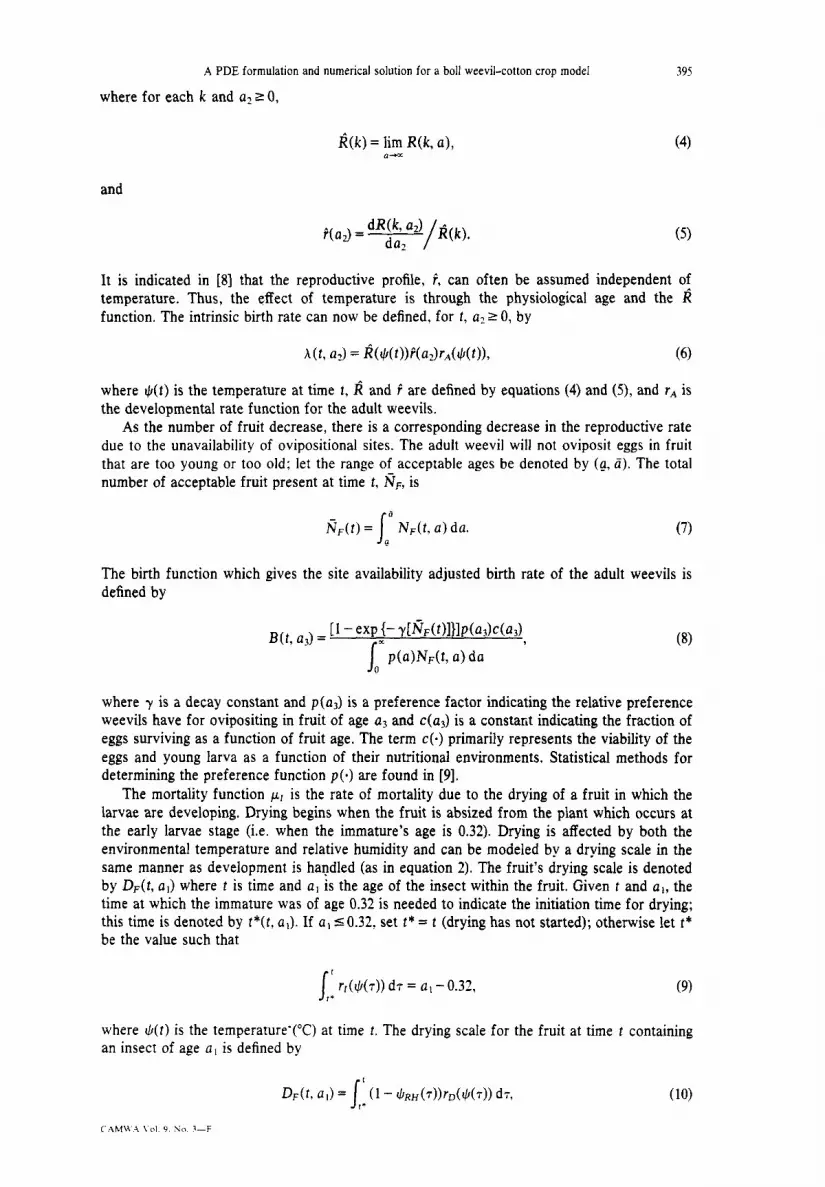
Fig. 2. Model comparisons with I%7 experimental data of Walker and Niles[l31 for large flower buds and

adult boll weevils.

(iv) For j E J,(n) and i E Jr(n)

Nr(t,+t, a1.i + Aat, Si) = Nr(tnt a~.j, Si>[l -Q(S(fn+tt a~,i + Aa,)/q(si))l

x [I- Ff(ai,,+ Aat)llI[l - @(fi(tm al,i)/v(si))l

x L1 - Fr(al,i)l17

where 0 is the distribution function used in equation (11).

(e) Increment n and return to step (b).

Figures 1 and 2 indicate the appropriateness of this modeling approach. The experimental field

data are for the years 1966 and 1967 from a study of Walker and Niles[l3]. The figures compare

the model and field data for the total number of preferred ovipositional sites (floral buds larger than

7 mm dia.) and adult weevils on a per acre (0.405 hectare) basis. However the data was collected

on a l/22 acre (183.95 m’) plots so there is considerable variation in the counts especially in the

low numbers. The immigration numbers of overwintering weevils are especially variable so the

major method of fitting the model to the data was to adjust the immigration rates. The

proportion of females in the overwintering influxes was 75% whereas the normal population

proportions are 50%. There were also slight differences in soil moisture conditions of the crop

for the 1966 and 1967 seasons. Therefore some of the plant characteristics have been adjusted

slightly. All of the numerical values used in generating the model predictions are given in the

Appendix.

Acknowledgements-This work was funded in part by the multiuniversity research program “Consortium for Integrated

Pect Management” through an EPA Grant No. CR8Of1277030 and a USDA Grant No. 82-CRSR-2-1000.

1.

2.

3.

4.

5.

6.

7.

8.

9.

10.

11. zyxwvutsrqponmlkjihgfedcbaZYXWVUTSRQPONMLKJIHGFEDCBA

13

T. R. Malthus, An zyxwvutsrqponmlkjihgfedcbaZYXWVUTSRQPONMLKJIHGFEDCBAEssay on the Principle of Population. Reeves & Turner, London (Reprinted 1976 by W. N. Norton & Company, New York, pp. 15-130) (1798). H. Von Foerster, In The Kinetics of Cellular Proliferation (Edited by F. Stohlman, Jr.), pp. 382-407. Grune & Stratton, New York (1959). Y. Wang. A. P. Gutierrez, G. Oster and R. Daxl, A general model for plant growth and development: coupling plant-herbivore interactions. Can. Entomol. 109, 1359-1374 (1977). G. L. Curry, R. M. Feldman, B. L. Deuermeyer and M. E. Keener, Approximating a closed-form solution for cotton fruiting dynamics. Math. Biosci. 54, 91-l 13 (1981). G. L. Curry, P. J. H. Sharpe, D. W. DeMichele and J. R. Cate, Towards a management model of the cotton-boll weevil

ecosystem. J. Enoiron. Management 11, 187-223 (1980). G. L. Curry, J. R. Cate and P. J. H. Sharpe, Cotton bud drying: contributions to boll weevil mortality. Enoiron. Entomol. 11, 344-350 (1982). G. Oster, In Some MathemaIical Questions in Biology VII (Edited by S. A. Levin), pp. 37-68. Symposium on Mathematical Biology, The American Mathematical Society, Providence, Rhode Island (1976). G. L. Curry, R. M. Feldman and K. C. Smith, A stochastic model of a temperature-dependent population. Theor. Pop. Biol. 13. 197-213 (1978). J. R. Cate, G. L. Curry and R. M. Feldman, A model for boll weevil ovipositional site selection. Enuiron. Entomol. 8, 917-921 (1979). D. W. DeMichele, G. L. Curry, P. J. H. Sharpe and C. S. Barlield, Cotton bud drying: a theoretical model. Enoiron.

Entomol. 5, 1011-1016 (1976). G. L. Curry, R. M. Feldman, P. J. H. Sharpe, Foundations of stochastic development. J. Theor. Biol. 74, 397-410 (1978).

._. R. E. Barlow and F. Proschan, Stntisticnl Theory of Reliability and Life Testing. Holt, Rinehart & Winston, New York

(1975).

A PDE formulation and numerical solution for a boll weevil-cotton crop model 401

REFERENCES

13. J. K. Walker, Jr. and G. A. Niles, Population dynnmics of the boll weevil and modified cotton types: implications for

pest management. Texas Agric. Exp. Sta. Bull., No. 1109 (1971).

Dejnirions and numerical values

APPENDIX

The numerical values for the parameters and functions used in the model are listed below in alphabetical order. The variables aI. a?, and a3 refer to the physiological age of immature insects, adult insects, and fruit, respectively. In the function definitions the functional values are assumed zero outside the indicated limits of the independent variables. If no domain is given, then it is assumed to be the nonnegative reals. Temperature data is from the airport at College Station, Texas which is located adjacent to the experimental plot. A sinusoidal curve was fit through daily min-max temperatures in order to obtain hourly temperatures throughout the day. The study in 1%6 began on Julian day 168 and the I%7 study on day 15 1. The chronological time increment size was one day and developmental rates were computed using an hourly grid (i.e. At = 1, m = 24). The parameter values used for all the model data follow:

a*: lower age for forced shedding of fruit.

a*=035 . .

c: fraction immatures surviving through first instar larvae

da31 = 1 i:$ z: z 0”:: (Flowering occurs at a3 = 0.4).

d: photosynthate demand

d(at) = [- 0.4628203 + 25.232as’- 181.42a: + 606.520: - 957.83aJ5 + 700.86aj6- 192.68a:J+.

Fa: probability distribution function for adult longevity

FA(a2) = I- eXp {-a*}.

FE: probability distribution function for immature emergence as an adult

Fe(a,) = 65.191/a,‘- 195.575/a,* t 190.783/a] -59.899

for 0.86475 a, 5 1.1856. p: preference weighting factor

i

0.386 0 I a3 CO.24

p(a3)= 1.0 0.24 5 a3 < 0.4

0.54 03 z 0.4.

d: total reproductive capacity of an adult weevil

I?(k) = - 14319+4226.2k -493.9lk’t 29.223k” -0.92449k4 t 0.014926k5-9.6805 x lo-‘k”

for 17°C s k s 39°C. i: reproductive density function

i(x) dx = 0.44605 - 2.5399~ + 4.7617a2’ - 3.691Sa?‘+ l.7121a~-0.50751a~5+0.088413a~-0.0067772a~

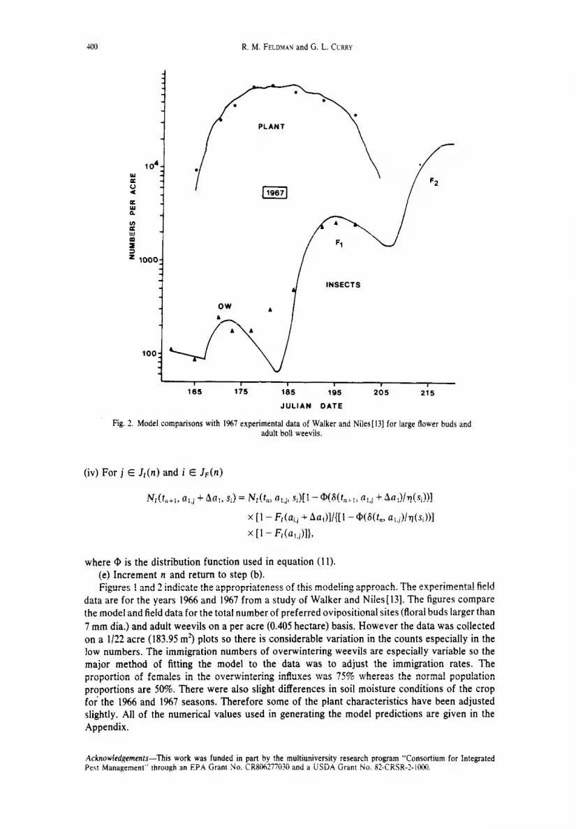
402 R. M. FELDMAN and G. L. CCRRY

for 0.5 14 I a> I 3.08. r.4: adult insect developmental rate

r&) = I (k-11)/131 for ll”C1k<35”C

0.18321 for zyxwvutsrqponmlkjihgfedcbaZYXWVUTSRQPONMLKJIHGFEDCBAk 2 35°C.

ro: drying rate for immature mortality

r,,(k) = (8.38 x lO’/k) em”‘” 5/i

where E = 273 + k and k is “C. r~: fruit developmental rate

W(k) = (k-11)/982 for ll”C~k<35”C

0.02444 for k z 35°C.

rr: immature insect developmental rate zyxwvutsrqponmlkjihgfedcbaZYXWVUTSRQPONMLKJIHGFEDCBA

n(k) = (f/5720) exp {27.44- 8176.35/c}

1 +exp{-344+99047/k}+exp{l16.4-35855/c}

where E = 273 + k and k is “C. S: photosynthate supply

s 1.26 _ for 1966 plot

1.2 for I%7 plot.

p: maximum bud initiation rate

9.55/age unit for 1966 plot

’ = (l0.*3/age unit for I%7 plot.

y: decay factor for availability of ovipositional sites

y = - 1.1714X IO-‘/acre.

7: critical number indicating death due to drying

q(s) = s’/6 t (0.2415)‘/3s -(0.2415)‘/2

for s L 0.2415 cm. cc: natural shedding of fruit

p(a3) =

O.l9/age unit for 1966 plot

O.ZO/age unit for I%7 plot

for 0 5 a3 5 0.83. p: immigration rate

Immigration occurs at the start of the season only. Daily immigration for the 1966 plot was 20/day for the first 12 days followed by single days of 15, IO, then 5. Daily immigration for I%7 plot was four zeros, followed by 6 days of 25/day, than 7 days of IO/day, then 3 days of 60/day, followed by 50,40, 30,20, then 10. The age of these overwintering weevils was set at 0.8 to account for their reduced reproductive capacity.

u: size of fruit (radius in cm)

2.333a3 for OIaj<0.12

0.857(& - 0.12) + 0.28 for 0.12 S a3 < 0.4

dad =. (a, - 0.4) + 0.52 for 0.4 S a3 < 0.44

6.3(a3 - 0.44) + 0.56 for 0.44 I a3 < 0.54

2.6(a3 - 0.54) + 1.19 for 0.54 5 a? < 0.57

1.27 for ai r0.57.