A new approach for the computation of harmonics and interharmonics produced by AC/DC/AC conversion systems with PWM inverters

EUROPEAN TRANSACTIONS ON ELECTRICAL POWEREuro. Trans. Electr. Power 2010; 20:68–82Published online 2 November 2009 in Wiley InterScience
(www.interscience.wiley.com) DOI: 10.1002/etep.400
*CyE-

Co

A new approach for the computation of harmonics and interharmonics producedby AC/DC/AC conversion systems with PWM inverters

Roberto Langella1*,y, Adolfo Sollazzo2 and Alfredo Testa1

1Department of Information Engineering, 2nd University of Naples, Aversa, Italy2CIRA–Italian Aerospace Research Centre, Caplia, Italy

SUMMARY

The computation of harmonics and interharmonics produced by AC/DC/AC conversion systems with PWM inverters is considered, and a newapproach is presented. Basically, a new inverter model is introduced that is based on the modulation function theory and is able to take into accountthe voltage ripple at the inverter input terminals. A rectifier model that was previously proposed and the new inverter model are first used in theframework of a direct injection procedure and, then, in an iterative harmonic and interharmonic analysis. The proposed model can be appliedsuccessfully to adjustable speed drives for asynchronous motors, achieving better modeling accuracy with respect to approaches based onsimplified inverter modeling. They also allow a sensible reduction of computational burden with respect to the time-domain models. For thisreason, they constitute an attractive tool inside Monte Carlo simulations for probabilistic analyses of harmonic and interharmonic distortion.Numerical experiments demonstrate the good performance of the proposed models and the need to account for the presence of interharmonics forhigh-power PWM drives. Copyright # 2009 John Wiley & Sons, Ltd.

key words: harmonics; interharmonics; modulation functions; power converters; PWM

1. INTRODUCTION

The computation of the harmonics and interharmonics produced by AC/DC/AC conversion systems is the object of extensive

research activity [1–10]. In addition to the typical problems caused by harmonics, such as overheating and the reduction of useful

life, interharmonics create several new problems, such as sub-synchronous oscillations, voltage fluctuations, and light flicker, even

for low-amplitude levels [10]. Typically, attention is devoted to those systems in which both AC/DC and DC/AC conversions are

operated by line commutated converters at different frequencies that intermodulate originating interharmonics; this is the case of

HVDC systems [3,4] and high-power adjustable speed drives (ASDs) [1]. Less attention has been devoted to different systems, such

as ASDs using PWM inverters, due to the assumption that the DC-link capacitor, which was used in this case, practically reduces the

intermodulation between the two converters to zero [5,6]. The interharmonics produced by PWMASDs are considered negligible in

Reference [6,7], independently on the drive power or on the working point for a given drive. The authors of Reference [8] took into

account the effects of the inverter on the DC–link capacitor voltage by means of an analytical approach that determines the currents

absorbed by the inverter based on the hypotheses that the rectifier commutation effects can be ignored and that the voltage

drops across the AC supply system can be considered as negligible.

Assumptions such as those assumed by the authors of Reference [8] can be accepted for high-short-ratio circuits and when the

conditions between the impedances of the AC system and the conversion system are far from a resonance condition. It is worth

noting that commercial simulation programs based on frequency scan analyses use these hypotheses. On the other hand, simulation

software based on time-domain modeling is also able to account for non-ideal conditions but requires a prohibitively long time for

the execution for instance of probabilistic analyses.

orrespondence to: Roberto Langella, 2nd University of Naples, Italy Information Engineering, Aversa, Italy.mail: [email protected]

pyright # 2009 John Wiley & Sons, Ltd.

COMPUTATION OF HARMONICS AND INTERHARMONICS 69

Based on the introduction of four auxiliary switches that are able to model both the rectifier and the inverter, the authors of

Reference [1] proposed an iterative approach (IA) to model line commutated AC/DC/AC conversion systems that was able to take

into account interactions between the AC supply system and the conversion system. The model was very fast, which meant that its

use inside Monte Carlo simulations for probabilistic modeling of harmonic and interharmonic distortion was very effective [11].

In this paper, the authors develop a model for the case of the PWM inverter with features similar to those of the model proposed in

Reference [1]. A preliminary proposal of this model [12] showed the importance of the interaction between the AC supply system

and the conversion system close to resonance conditions, when an accurate evaluation of interharmonic distortion is needed.

Experimental validation of this preliminary proposal was conducted with very good results. The validation used experimental data

measured on a high speed locomotive for the Italian railway system [13].

The proposed approach can be used by engineers, e.g., to avoid dangerous resonance conditions in the design stage of electrical

industrial systems, including AC/DC/AC conversion systems; to prevent interference problems with signaling systems for instance

in railway applications; and to assess the expected life of power system components in the presence of distorted waveforms by

means of probabilistic analyses.

In the following sections, the rectifier model proposed in Reference [1] is recalled, and the new model of the PWM inverter is

presented and discussed. Then, the new approach to modeling the AC/DC/AC conversion system is described in detail. First,

the rectifier model and the PWM inverter model are used in the framework of a direct injection procedure and, then, inside a

procedure based on the iterative harmonic and interharmonic analysis [14–15]; a compensation technique [16] is also used to

improve the convergence characteristics of the IHIAFinally, some comparative numerical experiments show the characteristics of

the proposed approach and the necessity of accounting for interharmonics in case of high-power PWM drives.

2. THE CONVERTERS MODEL

The typical scheme of a PWM ASD is shown in Figure 1. In this kind of system, the PWM inverter controls the output voltages

properly, both in terms of amplitude and frequency, depending on the working conditions and on the power consumption of the load,

so a simple diode bridge is enough to rectify the input voltages of the three-phase supply system.

2.1. Rectifier

The rectifier can be modeled by means of the circuit presented in Reference [1] and shown in Figure 2, where, for the sake of

simplicity, a resistive-inductive (RSS, LSS) structure for the equivalent of the supply system is considered. More generally, the

equivalent circuit of the supply system can be modeled by a generic equivalent that can be obtained, for example, starting from field

measurements.

Figure 1. AC/DC/AC conversion system with PWM inverter.

Figure 2. Three-phase rectifier; (a) scheme, (b) model.

Copyright # 2009 John Wiley & Sons, Ltd. Euro. Trans. Electr. Power 2010; 20:68–82

DOI: 10.1002/etep

70 R. LANGELLA, A. SOLLAZZO AND A. TESTA

The voltage vdcr (t) is calculated by:

vdcr tð Þ ¼ Sva tð Þ � va tð Þ þ Svb tð Þ � vb tð Þ þ Svc tð Þ � vc tð Þ; (1)

where Sva (t), Svb (t), and Svc (t) are proper voltage modulation functions [1,3,4,19]. Modulation functions are the relationships

among inputs and outputs of a converter that can be seen as a modulator during its operation. For instance the voltage modulation

function of a single-phase bridge rectifier in ideal conditions assumes the value ‘þ1’ during the fundamental positive half cycle of

the voltage and ‘�1’ for the rest of the cycle.

Two auxiliary switches, SwE1 and SwE2, make it possible to take the rectifier commutation into account. They are operated by the

switching functions, SE1 (t) and SE2 (t). SE1 (t) assumes a value of 1 when the rectifier is commutating, whereas SE2 (t) assumes value

of 1 when the rectifier is conducting; otherwise, they assume null values. During the commutation, the equivalent impedance as seen

from the DC-link is 1.5 times the phase impedance of the supply system side, whereas it is a factor of 2 larger during the conduction

stage [1].

The current idcr (t) can be calculated only after a proper DC equivalent load has been assumed, as will be shown in the following

sub-sections III.B and III.C. (See circuits of Figures 5 and 7.)

2.2. PWM inverter

The scheme of a three-phase voltage source inverter that, for the sake of simplicity, supplies a resistive-inductive active AC load is

shown in Figure 3a). The control strategy of the power switches is obtained by means of the PWM technique [17]. Usually, these

types of inverters are modeled by means of a current generator. (See Figure 3b).)

In Reference [5], a simple model was proposed considering only the DC component, Idci, of the current absorbed by the inverter

idci (t). This is calculated starting from the knowledge of the load power consumption, P, and the DC component of the voltage at the

inverter input terminals, Vo’o:

Idci ¼P

Vo0o: (2)

In Reference [18], an improved model was proposed taking into account also the harmonics of the current absorbed by the

inverter. Starting from the relationship between the instantaneous DC link and load power, it is possible to calculate the current

absorbed by the inverter, after making the assumption that the voltage at the inverter input terminals only has the DC component,

Vo’o:

idciðtÞ ¼vANðtÞiAðtÞ

Vo0oþ vBNðtÞiBðtÞ

Vo0oþ vCNðtÞiCðtÞ

Vo0o: (3)

A similar model was used in Reference [6], and the line-to-neutral voltages are calculated by means of three switching functions:

vANðtÞ ¼ Vo0oSANðtÞ; vBNðtÞ ¼ Vo0oSBNðtÞ; vCNðtÞ ¼ Vo0oSCNðtÞ: (4)

The generic switching function, SjN (t), and the load current, ij (t), with j¼A, B, and C, are considered as double-sided infinite

sums with a fundamental frequency equal to the operating frequency of the inverter [6]. Both the series are truncated after a

reasonable number of terms.

Figure 3. Three-phase voltage source inverter; (a) scheme, (b) model.


DOI: 10.1002/etep


In Reference [8], Equations (4) were used by substituting the voltage Vo’o with time-dependent voltages obtained starting from

no-load supply voltages multiplied by ideal switching functions that ignore the rectifier commutation.

In the proposed new model, the interactions between supply and supplied sides are modeled also taking into account the ripple of

the voltage at the inverter input terminals that is due to the effects of the rectifier commutation and of the voltage drops caused by the

load and capacitor currents.

In particular, the voltages vAN (t), vBN (t), and vCN (t) are evaluated starting from vAO (t), vBO (t), and vCO (t), defined with reference

to Figure 3a). Assuming the AC load is balanced, it is:

vANðtÞvBNðtÞvCNðtÞ

24

35 ¼

þ2=3 �1=3 �1=3�1=3 þ2=3 �1=3�1=3 �1=3 þ2=3

24

35 �

vAOðtÞvBOðtÞvCOðtÞ

24

35: (5)

vAO (t), vBO (t), and vCO (t) are evaluated by multiplying vo’o (t) by proper switching functions SAO (t), SBO (t), and SCO (t) that are the

control signals of the upper switches Sw1, Sw2, and Sw3:

vAOðtÞ ¼ SAOðtÞ � vo0oðtÞ; vBOðtÞ ¼ SBOðtÞ � vo0oðtÞ; vCOðtÞ ¼ SCOðtÞ � vo0oðtÞ; (6)

where vo’o (t) is obtained by the model described in Section III, below. The current absorbed by the inverter is calculated by means of

the formula:

idciðtÞ ¼ SAOðtÞiAðtÞ þ SBOðtÞiBðtÞ þ SCOðtÞiCðtÞ: (7)

This equation is similar to Equation (3) when Vo’o is replaced by vo’o (t), and iA (t), iB (t), and iC (t) are obtained by applying the

concept of the inverse discrete Fourier transform to their spectral components:

Ik

A ¼ Vk

AN � Ek

A

R þ jkvFL; I

k

B ¼ Vk

BN � Ek

B

R þ jkvFL; I

k

C ¼ Vk

CN � Ek

C

R þ jkvFL; (8)

where Vk

ðÞandEk

ðÞ are the kth components of v() (t) and e() (t) of Figure 3a), respectively. The e.m.f. e() (t) can be preliminarily

estimated by starting from experimental measurements or by simplified time-domain simulations performed for a reduced number

of reference working conditions.

More general expressions can be used instead of Equation (7), when the inverter load is represented by a more general model [1].

3. ENTIRE SYSTEM MODEL

Combining the model developed in section II for the rectifier and for the inverter and including a proper DC-link representation

allow modeling the entire system. Two models are described in the following sub-sections. The first refers to a Direct Approach that

solves thewhole system in two steps, and the latter is an IA that requires a recursive solution to be iterated until a proper convergence

criterion is satisfied.

3.1. Direct approach

In a first step, the harmonic and interharmonic components of the currents at the inverter input and output sides are calculated by

applying Equations (7) and (8) for the model described in II.B, starting from an estimation of the voltage at the inverter input

terminals, vo’o (t), evaluated considering only the harmonics due to the rectifier.

In a second step, reference is made to the circuit in Figure 2b). The direct DC Equivalent Load is obtained by replacing the current

generator calculated at the end of the first step in parallel with the filter capacitor with the Thevenin equivalent, as illustrated in

Figure 4; the series part of the DC filter, Rdc and Ldc, remains unaffected. The circuit illustrated in Figure 5 is finally obtained.

The current at the rectifier output side is:

idcrðtÞ ¼ Idcr þ DidcrðtÞ; (9)


DOI: 10.1002/etep

Figure 4. Thevenin equivalent operated at the inverter input terminals.

Figure 5. Circuit for the calculation of rectifier DC side ripple current.


where Idcr coincides with the DC component of the current at the inverter input side, idci (t), (see Equation (7)), and the rectifier DC

side ripple current, Didcr (t), is obtained as proposed in Reference[1] starting from the solution of the circuit in Figure 5 evaluated by

applying the superposition principle to the two loops that are present:

DidcrðtÞ ¼X2j¼1

XN

k¼1

Vk

jdc

Zk

Ej

�� sinðkvFt þ ’

Vk

jdc�Z

k

Ej

� �Þ (10)

where vF is the Fourier fundamental frequency [1], and Vk

jdcis the kth component of the voltage

vjdcðtÞ ¼ ðvdcrðtÞ � eo0oðtÞÞ SEjðtÞ with j ¼ 1; 2; (11)

and

Zk

E1 ¼ ð1:5RSS þ RdcÞ þ ikvFð1:5LSS þ LdcÞ þ 1=ðikvFCdcÞ;

Zk

E2 ¼ ð2RSS þ RdcÞ þ ikvFð2LSS þ LdcÞ þ 1=ðikvFCdcÞ:(12)

Finally, the rectifier input side currents are calculated by using the rectifier current switching functions Sia, Sib, and Sic [1]:

ia tð Þ ¼ Sia tð Þ � idcr tð Þ; ib tð Þ ¼ Sib tð Þ � idcr tð Þ; ic tð Þ ¼ Sic tð Þ � idcr tð Þ: (13)

This approach takes into account the inverse modulating effect of the rectifier.

The results obtained in several working conditions for the case study illustrated in Vare acceptable in the majority of cases. But,

for those operating points for which the interactions between the two conversion systems are amplified by the resonance

phenomenon caused by the DC filter, the inaccuracies associated with the interharmonic components become unacceptable. This is

typical of the direct solution technique because it does not take the interactions between the load (inverter) and the supply (rectifier)

circuits into account.

3.2. Iterative approach

For the problems described in the previous sub-section, the authors decided to use the IHIA procedure that is described in the following

part of this section. This procedure uses the Parallel Compensation Technique [18] to improve its convergence characteristics.

Figure 6 shows the structure of the DC equivalent circuit that represents the whole AC/DC/AC conversion system of Figure 1.


DOI: 10.1002/etep

Figure 6. Circuit for the implementation of the iterative approach.


The system is divided into two sections, and the voltage at the inverter DC terminals O’-O (Figure 2) is chosen as an observation

variable for the convergence check.

The physical system is modified by the addition of a pair of equal and opposite parallel compensation impedances. The

combination of these impedances amounts to an infinite value impedance and ensures that the physical system being studied remains

unaffected by the addition. The positive impedance, + Z, is absorbed in the left-side section, while the negative impedance, �Z,

originates a new, modified, non-linear load along with the inverter and its load. In Reference [16], it was demonstrated that the

compensation operated by the impedances + Z and �Z improves convergence characteristics and avoids the lack of convergence,

caused by impedance resonances, by a proper choice of Z.

In the left-side section, Zeq is the equivalent impedance, which takes into account the series of DC-link inductance and resistance

and the average supply side impedance seen by the DC side. This impedance involves both the conduction and the commutation

conditions, so it depends on their duration, i.e., the overlapping angle m [1].

The steps of the iterative procedure are:

Co

(1) c

pyrig

alculation of the voltage harmonic source vdcr (t) by Equation (1) assuming initial values for va (t), vb (t), and vc (t) equal

to ea (t), eb (t), and ec (t), respectively, or values estimated assuming proper initial values for ia (t), ib (t), and ic (t);

(2) c
alculation of the voltage vo’o (t) solving the circuit of Figure 6, assuming the right-side section to be disconnected;
(3) c
alculation of the current idci (t) by Equation (7);
(4) c
alculation of the spectral components of the current, iRS (t), absorbed by the right-side section:
Ik

RS ¼ Ik

dci þV

k

o0o

�Zk; (14Þ

where Ik

dci is the kth component of the current idci (t), Vk

o0o is the kth component of the voltage vo’o (t), and�Zk is the negative

compensation impedance at the angular frequency kvF;

(5) c
alculation of voltage drop Dvo’o (t), obtained by injecting the current iRS (t) in the Thevenin equivalent impedance of the
left-side section, ZkeqLS, starting from its spectral components:

DVk

o0o ¼ ZkeqLS � I

k

RS; (15Þ
(6) u pdating the voltage vo’o (t) for the (i+ 1)th iteration, starting from its components:
ðVk

o0oÞiþ1 ¼ ðVk

o0oÞi � DVk

o0o; (16)

where ðVk

o0oÞi is the kth component of the voltage used in steps 3 and 4 of the current ith iteration.

Steps 3 through 6 are iterated until no significant variations are found for any of the components of the voltage vo’o (t).

Once the circuit of Figure 6 has been solved, the rectifier-output-side current can be calculated.

A first possibility is to apply the formula:

Ik

dcr ¼V

k

dcr � Vk

o0o

Zkeq

; (17)

which solves the left-side section of the circuit in terms of idcr (t) spectral components. This means to assume the mean value for

the Zeq previously defined, so ignoring the modulation effects of the alternating of the rectifier conduction and commutation

conditions [1].

ht # 2009 John Wiley & Sons, Ltd. Euro. Trans. Electr. Power 2010; 20:68–82

DOI: 10.1002/etep

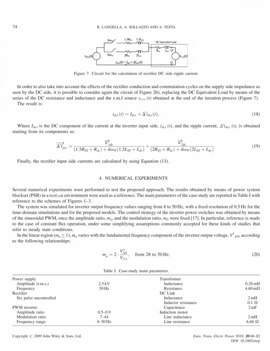
Figure 7. Circuit for the calculation of rectifier DC side ripple current.


In order to also take into account the effects of the rectifier conduction and commutation cycles on the supply side impedance as

seen by the DC side, it is possible to consider again the circuit of Figure 2b), replacing the DC Equivalent Load by means of the

series of the DC resistance and inductance and the e.m.f source vo’o (t) obtained at the end of the iteration process (Figure 7).

The result is:

idcrðtÞ ¼ Idcr þ D0idcrðtÞ; (18)

Where Idcr is the DC component of the current at the inverter input side, idci (t), and the ripple current, D’idcr (t), is obtained

starting from its components as:

D0Ik

dcr ¼V

k

1dc

ð1:5RSS þ RdcÞ þ ikvFð1:5LSS þ LdcÞþ V

k

2dc

ð2RSS þ RdcÞ þ ikvFð2LSS þ LdcÞ: (19)

Finally, the rectifier input side currents are calculated by using Equation (13).

4. NUMERICAL EXPERIMENTS

Several numerical experiments were performed to test the proposed approach. The results obtained by means of power system

blockset (PSB) in a MATLAB environment were used as a reference. The main parameters of the case study are reported in Table I with

reference to the schemes of Figures 1–3.

The system was simulated for inverter output frequency values ranging from 8 to 50Hz, with a fixed resolution of 0.5 Hz for the

time-domain simulations and for the proposed models. The control strategy of the inverter power switches was obtained by means

of the sinusoidal PWM, once the amplitude ratio, ma, and the modulation ratio, mf, were fixed [17]. In particular, reference is made

to the case of constant flux operation, under some simplifying assumptions commonly accepted for these kinds of studies that

refer to steady state conditions.

In the linear region (ma� 1), ma varies with the fundamental frequency component of the inverter output voltage, V1AN, according

to the following relationships:

ma ¼ 2 � V1AN

Vo0o; from 28 to 50Hz; (20)

Table I. Case-study main parameters.

Power supply TransformerAmplitude (r.m.s.) 2.5 kV Inductance 0.28mHFrequency 50Hz Resistance 4.60mV

Rectifier DC LinkSix pulse uncontrolled Inductance 2mH

Inductor resistance 0.1 VPWM inverter Capacitance 2mFAmplitude ratio 0.5–0.9 Induction motorModulation ratio 7–44 Line inductance 2mHFrequency range 8–50Hz Line resistance 6.66 V


DOI: 10.1002/etep


and

ma ¼ 0:5; from 8 to 27:5 Hz: (21)

The choice of mf is made according to the synchronous PWM, in which the triangular waveform signal and the sinusoidal control

signals are synchronized. This means that mf must be an integer. For this reason, the frequency of the triangular waveform signal,

i.e., the switching frequency, is not constant when the output frequency varies. The authors chose a maximum variation of �25Hz

around the nominal value of 350Hz.

A first comparison was performed among PSB, the direct approach (DA) of III.A, and the IA of III.B for two output frequencies of

the ASDs in order to highlight the effects of resonance phenomena produced by the interaction between the AC supply system and

the converter. In particular, an output frequency of 40Hz did not show critical conditions, while an output frequency of 12Hz

produced a resonance phenomenon as shown in the following part of this section.

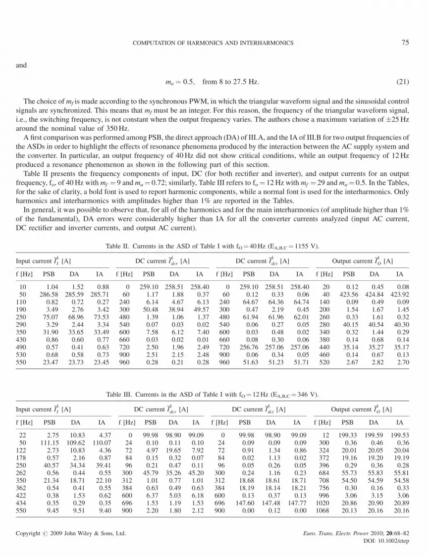
Table II presents the frequency components of input, DC (for both rectifier and inverter), and output currents for an output

frequency, fo, of 40Hz with mf ¼ 9 and ma¼ 0.72; similarly, Table III refers to fo¼ 12Hz with mf ¼ 29 and ma¼ 0.5. In the Tables,

for the sake of clarity, a bold font is used to report harmonic components, while a normal font is used for the interharmonics. Only

harmonics and interharmonics with amplitudes higher than 1% are reported in the Tables.

In general, it was possible to observe that, for all of the harmonics and for the main interharmonics (of amplitude higher than 1%

of the fundamental), DA errors were considerably higher than IA for all the converter currents analyzed (input AC current,

DC rectifier and inverter currents, and output AC current).

Table II. Currents in the ASD of Table I with fO¼ 40Hz (EA,B,C¼ 1155 V).

Input current Ik

I [A] DC current Ik

dcr [A] DC current Ik

dci [A] Output current Ik

O [A]

f [Hz] PSB DA IA f [Hz] PSB DA IA f [Hz] PSB DA IA f [Hz] PSB DA IA

10 1.04 1.52 0.88 0 259.10 258.51 258.40 0 259.10 258.51 258.40 20 0.12 0.45 0.0850 286.58 285.59 285.71 60 1.17 1.88 0.37 60 0.12 0.33 0.06 40 423.56 424.84 423.92110 0.82 0.72 0.27 240 6.14 4.67 6.13 240 64.67 64.36 64.74 140 0.09 0.49 0.09190 3.49 2.76 3.42 300 50.48 38.94 49.57 300 0.47 2.19 0.45 200 1.54 1.67 1.45250 75.07 68.96 73.53 480 1.39 1.06 1.37 480 61.94 61.96 62.01 260 0.33 1.61 0.32290 3.29 2.44 3.34 540 0.07 0.03 0.02 540 0.06 0.27 0.05 280 40.15 40.54 40.30350 31.90 33.65 33.49 600 7.58 6.12 7.40 600 0.03 0.48 0.02 340 0.32 1.44 0.29430 0.86 0.60 0.77 660 0.03 0.02 0.01 660 0.08 0.30 0.06 380 0.14 0.68 0.14490 0.57 0.41 0.63 720 2.50 1.96 2.49 720 256.76 257.06 257.06 440 35.14 35.27 35.17530 0.68 0.58 0.73 900 2.51 2.15 2.48 900 0.06 0.34 0.05 460 0.14 0.67 0.13550 23.47 23.73 23.45 960 0.28 0.21 0.28 960 51.63 51.23 51.71 520 2.67 2.82 2.70

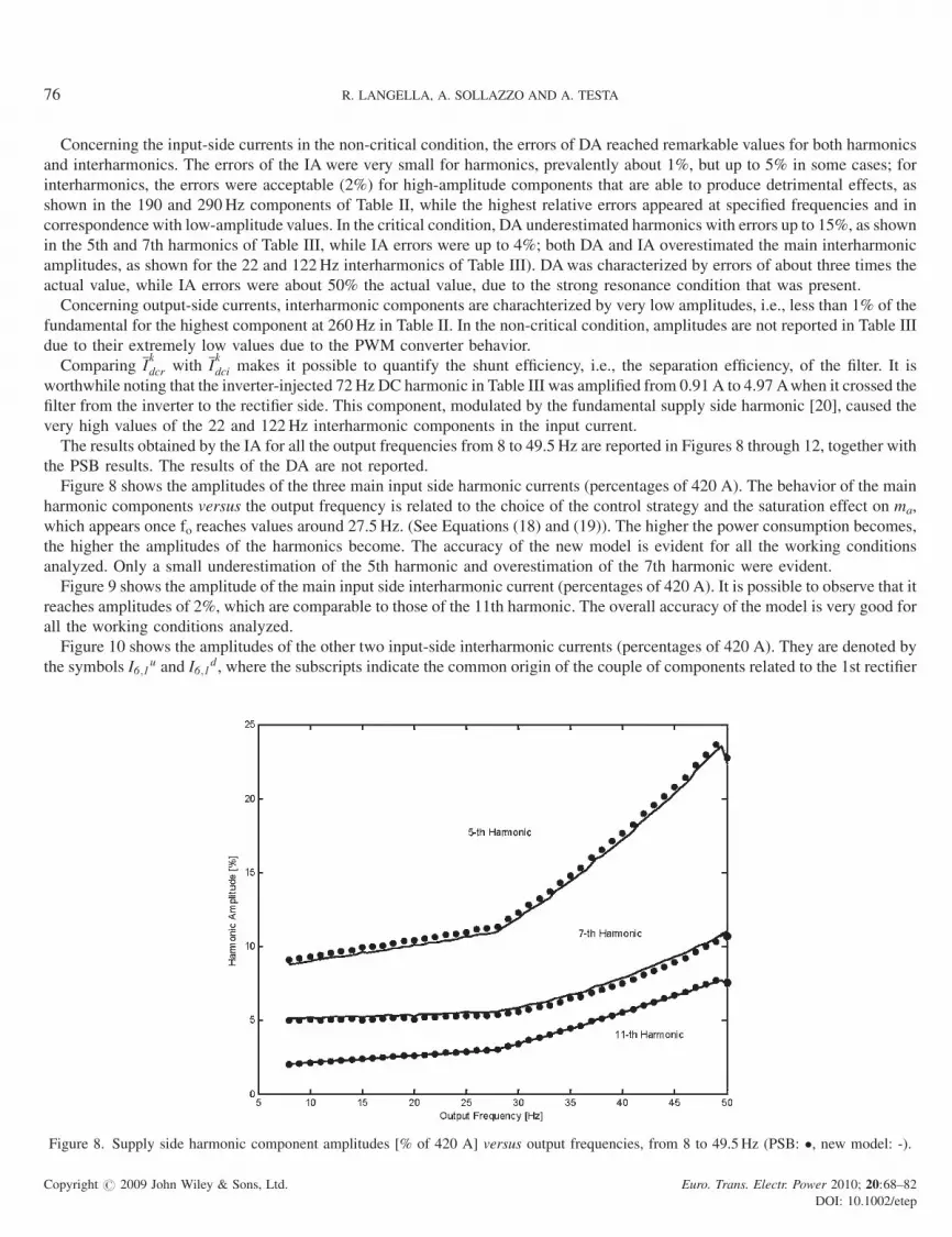
Table III. Currents in the ASD of Table I with fO¼ 12Hz (EA,B,C¼ 346 V).

Input current Ik

I [A] DC current Ik

dcr [A] DC current Ik

dci [A] Output current Ik

O [A]

f [Hz] PSB DA IA f [Hz] PSB DA IA f [Hz] PSB DA IA f [Hz] PSB DA IA

22 2.75 10.83 4.37 0 99.98 98.90 99.09 0 99.98 98.90 99.09 12 199.33 199.59 199.5350 111.15 109.62 110.07 24 0.10 0.11 0.10 24 0.09 0.09 0.09 300 0.36 0.46 0.36122 2.73 10.83 4.36 72 4.97 19.65 7.92 72 0.91 1.34 0.86 324 20.01 20.05 20.04178 0.57 2.16 0.87 84 0.15 0.32 0.07 84 0.02 1.13 0.02 372 19.16 19.20 19.19250 40.57 34.34 39.41 96 0.21 0.47 0.11 96 0.05 0.26 0.05 396 0.29 0.36 0.28262 0.56 0.44 0.55 300 45.79 35.26 45.20 300 0.24 1.16 0.23 684 55.73 55.83 55.81350 21.34 18.71 22.10 312 1.01 0.77 1.01 312 18.68 18.61 18.71 708 54.50 54.59 54.58362 0.54 0.41 0.55 384 0.63 0.49 0.63 384 18.19 18.14 18.21 756 0.30 0.16 0.33422 0.38 1.53 0.62 600 6.37 5.03 6.18 600 0.13 0.37 0.13 996 3.06 3.15 3.06434 0.35 0.29 0.35 696 1.53 1.19 1.53 696 147.60 147.48 147.77 1020 20.86 20.90 20.89550 9.45 9.51 9.40 900 2.20 1.80 2.12 900 0.00 0.12 0.00 1068 20.13 20.16 20.16


DOI: 10.1002/etep


Concerning the input-side currents in the non-critical condition, the errors of DA reached remarkable values for both harmonics

and interharmonics. The errors of the IA were very small for harmonics, prevalently about 1%, but up to 5% in some cases; for

interharmonics, the errors were acceptable (2%) for high-amplitude components that are able to produce detrimental effects, as

shown in the 190 and 290Hz components of Table II, while the highest relative errors appeared at specified frequencies and in

correspondence with low-amplitude values. In the critical condition, DA underestimated harmonics with errors up to 15%, as shown

in the 5th and 7th harmonics of Table III, while IA errors were up to 4%; both DA and IA overestimated the main interharmonic

amplitudes, as shown for the 22 and 122Hz interharmonics of Table III). DAwas characterized by errors of about three times the

actual value, while IA errors were about 50% the actual value, due to the strong resonance condition that was present.

Concerning output-side currents, interharmonic components are charachterized by very low amplitudes, i.e., less than 1% of the

fundamental for the highest component at 260Hz in Table II. In the non-critical condition, amplitudes are not reported in Table III

due to their extremely low values due to the PWM converter behavior.

Comparing Ik

dcr with Ik

dci makes it possible to quantify the shunt efficiency, i.e., the separation efficiency, of the filter. It is

worthwhile noting that the inverter-injected 72Hz DC harmonic in Table III was amplified from 0.91 A to 4.97 Awhen it crossed the

filter from the inverter to the rectifier side. This component, modulated by the fundamental supply side harmonic [20], caused the

very high values of the 22 and 122Hz interharmonic components in the input current.

The results obtained by the IA for all the output frequencies from 8 to 49.5 Hz are reported in Figures 8 through 12, together with

the PSB results. The results of the DA are not reported.

Figure 8 shows the amplitudes of the three main input side harmonic currents (percentages of 420 A). The behavior of the main

harmonic components versus the output frequency is related to the choice of the control strategy and the saturation effect on ma,

which appears once fo reaches values around 27.5Hz. (See Equations (18) and (19)). The higher the power consumption becomes,

the higher the amplitudes of the harmonics become. The accuracy of the new model is evident for all the working conditions

analyzed. Only a small underestimation of the 5th harmonic and overestimation of the 7th harmonic were evident.

Figure 9 shows the amplitude of the main input side interharmonic current (percentages of 420 A). It is possible to observe that it

reaches amplitudes of 2%, which are comparable to those of the 11th harmonic. The overall accuracy of the model is very good for

all the working conditions analyzed.

Figure 10 shows the amplitudes of the other two input-side interharmonic currents (percentages of 420 A). They are denoted by

the symbols I6;1u and I6;1

d, where the subscripts indicate the common origin of the couple of components related to the 1st rectifier

Figure 8. Supply side harmonic component amplitudes [% of 420 A] versus output frequencies, from 8 to 49.5Hz (PSB: �, new model: -).


DOI: 10.1002/etep

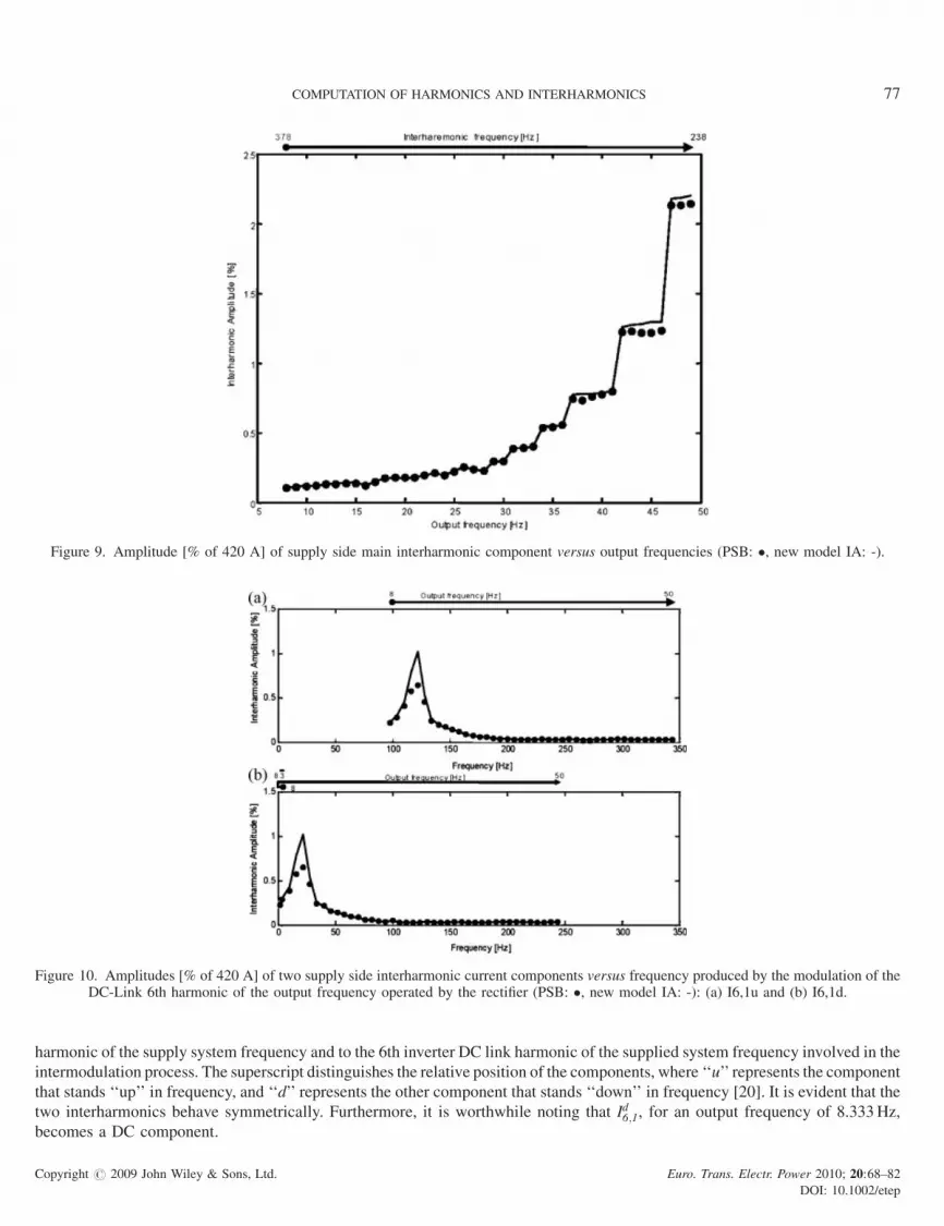
Figure 9. Amplitude [% of 420 A] of supply side main interharmonic component versus output frequencies (PSB: �, new model IA: -).

Figure 10. Amplitudes [% of 420 A] of two supply side interharmonic current components versus frequency produced by the modulation of theDC-Link 6th harmonic of the output frequency operated by the rectifier (PSB: �, new model IA: -): (a) I6,1u and (b) I6,1d.


harmonic of the supply system frequency and to the 6th inverter DC link harmonic of the supplied system frequency involved in the

intermodulation process. The superscript distinguishes the relative position of the components, where ‘‘u’’ represents the component

that stands ‘‘up’’ in frequency, and ‘‘d’’ represents the other component that stands ‘‘down’’ in frequency [20]. It is evident that the

two interharmonics behave symmetrically. Furthermore, it is worthwhile noting that Id6;1, for an output frequency of 8.333Hz,

becomes a DC component.


DOI: 10.1002/etep

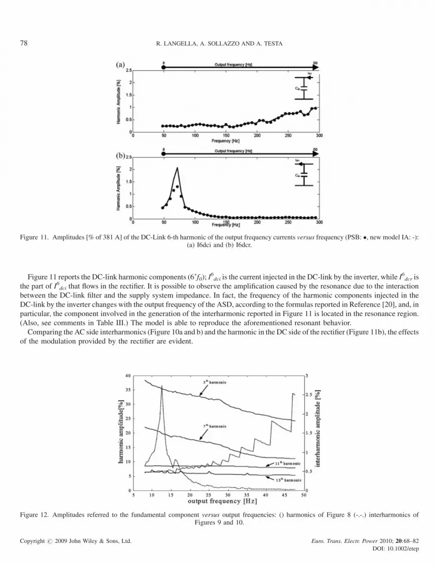
Figure 11. Amplitudes [% of 381 A] of the DC-Link 6-th harmonic of the output frequency currents versus frequency (PSB: �, new model IA: -):(a) I6dci and (b) I6dcr.


Figure 11 reports the DC-link harmonic components (6�f0); I6dci is the current injected in the DC-link by the inverter, while I6

dcr is

the part of I6dci that flows in the rectifier. It is possible to observe the amplification caused by the resonance due to the interaction

between the DC-link filter and the supply system impedance. In fact, the frequency of the harmonic components injected in the

DC-link by the inverter changes with the output frequency of the ASD, according to the formulas reported in Reference [20], and, in

particular, the component involved in the generation of the interharmonic reported in Figure 11 is located in the resonance region.

(Also, see comments in Table III.) The model is able to reproduce the aforementioned resonant behavior.

Comparing the AC side interharmonics (Figure 10a and b) and the harmonic in the DC side of the rectifier (Figure 11b), the effects

of the modulation provided by the rectifier are evident.

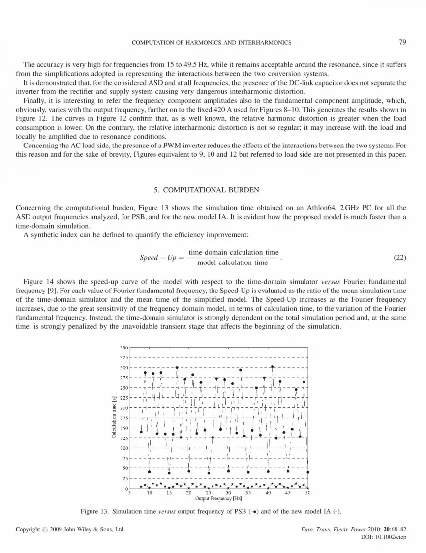
Figure 12. Amplitudes referred to the fundamental component versus output frequencies: () harmonics of Figure 8 (-.-.) interharmonics ofFigures 9 and 10.


DOI: 10.1002/etep


The accuracy is very high for frequencies from 15 to 49.5Hz, while it remains acceptable around the resonance, since it suffers

from the simplifications adopted in representing the interactions between the two conversion systems.

It is demonstrated that, for the considered ASD and at all frequencies, the presence of the DC-link capacitor does not separate the

inverter from the rectifier and supply system causing very dangerous interharmonic distortion.

Finally, it is interesting to refer the frequency component amplitudes also to the fundamental component amplitude, which,

obviously, varies with the output frequency, further on to the fixed 420 A used for Figures 8–10. This generates the results shown in

Figure 12. The curves in Figure 12 confirm that, as is well known, the relative harmonic distortion is greater when the load

consumption is lower. On the contrary, the relative interharmonic distortion is not so regular; it may increase with the load and

locally be amplified due to resonance conditions.

Concerning the AC load side, the presence of a PWM inverter reduces the effects of the interactions between the two systems. For

this reason and for the sake of brevity, Figures equivalent to 9, 10 and 12 but referred to load side are not presented in this paper.

5. COMPUTATIONAL BURDEN

Concerning the computational burden, Figure 13 shows the simulation time obtained on an Athlon64, 2GHz PC for all the

ASD output frequencies analyzed, for PSB, and for the new model IA. It is evident how the proposed model is much faster than a

time-domain simulation.

A synthetic index can be defined to quantify the efficiency improvement:

Speed � Up ¼ time domain calculation time

model calculation time: (22)

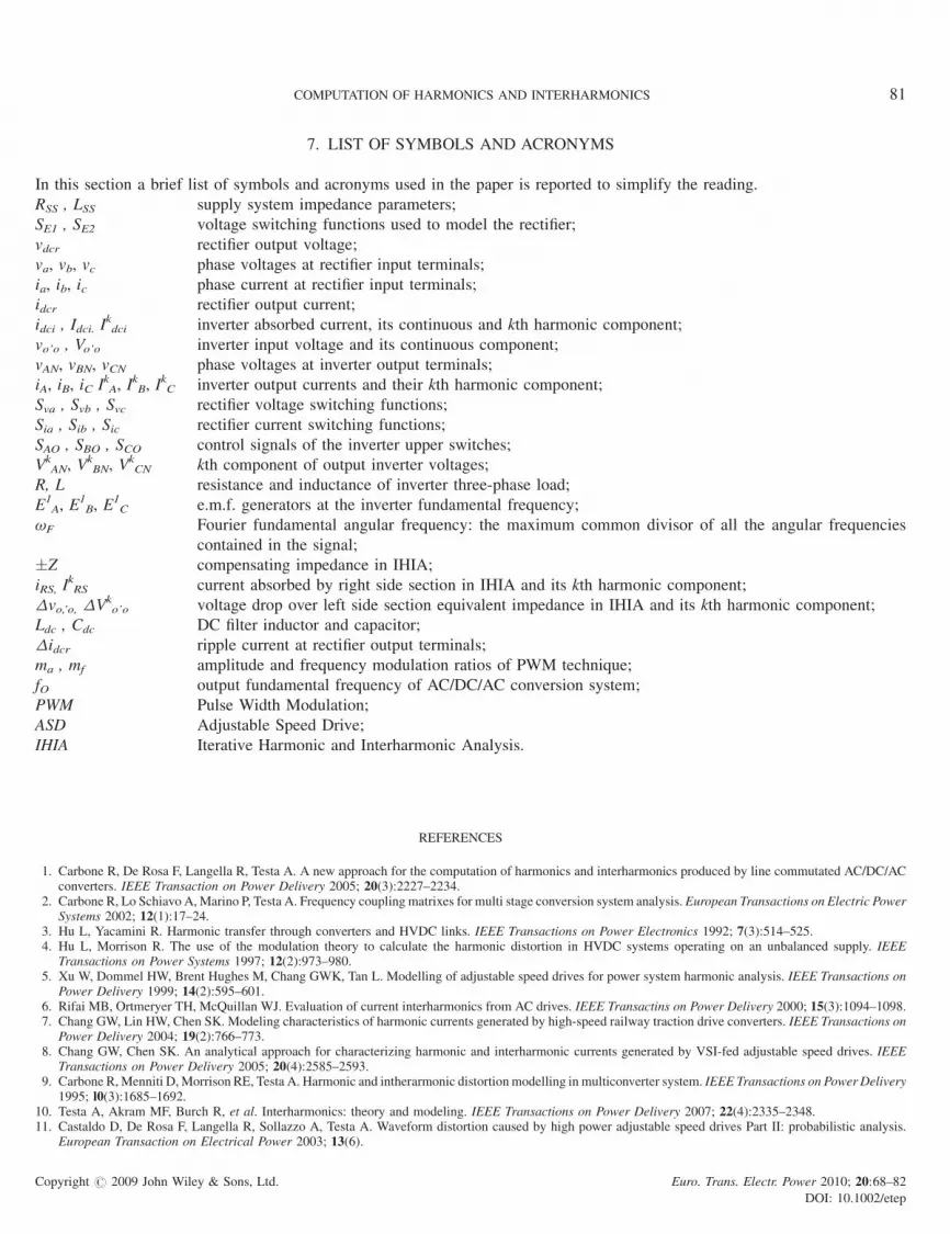
Figure 14 shows the speed-up curve of the model with respect to the time-domain simulator versus Fourier fundamental

frequency [9]. For each value of Fourier fundamental frequency, the Speed-Up is evaluated as the ratio of the mean simulation time

of the time-domain simulator and the mean time of the simplified model. The Speed-Up increases as the Fourier frequency

increases, due to the great sensitivity of the frequency domain model, in terms of calculation time, to the variation of the Fourier

fundamental frequency. Instead, the time-domain simulator is strongly dependent on the total simulation period and, at the same

time, is strongly penalized by the unavoidable transient stage that affects the beginning of the simulation.

Figure 13. Simulation time versus output frequency of PSB (-�) and of the new model IA (-).


DOI: 10.1002/etep

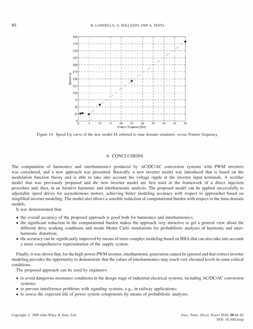
Figure 14. Speed-Up curve of the new model IA referred to time domain simulator, versus Fourier frequency.


6. CONCLUSIONS

The computation of harmonics and interharmonics produced by AC/DC/AC conversion systems with PWM inverters

was considered, and a new approach was presented. Basically, a new inverter model was introduced that is based on the

modulation function theory and is able to take into account the voltage ripple at the inverter input terminals. A rectifier

model that was previously proposed and the new inverter model are first used in the framework of a direct injection

procedure and, then, in an iterative harmonic and interharmonic analysis. The proposed model can be applied successfully to

adjustable speed drives for asynchronous motors, achieving better modeling accuracy with respect to approaches based on

simplified inverter modeling. The model also allows a sensible reduction of computational burden with respect to the time-domain

models.

It was demonstrated that:

Co

� th

py

e overall accuracy of the proposed approach is good both for harmonics and interharmonics;

� th
e significant reduction in the computational burden makes the approach very attractive to get a general view about the
different drive working conditions and inside Monte Carlo simulations for probabilistic analyses of harmonic and inter-

harmonic distortion;

� th
e accuracy can be significantly improved by means of more complex modeling based on IHIA that can also take into account
a more comprehensive representation of the supply system.

Finally, it was shown that, for the high-power PWM inverter, interharmonic generation cannot be ignored and that correct inverter

modeling provides the opportunity to demonstrate that the values of interharmonics may reach very elevated levels in some critical

conditions.

The proposed approach can be used by engineers:

� to
avoid dangerous resonance conditions in the design stage of industrial electrical systems, including AC/DC/AC conversion
systems;

� to
prevent interference problems with signaling systems, e.g., in railway applications;
� to
assess the expected life of power system components by means of probabilistic analyses.
right # 2009 John Wiley & Sons, Ltd. Euro. Trans. Electr. Power 2010; 20:68–82

DOI: 10.1002/etep


7. LIST OF SYMBOLS AND ACRONYMS

In this section a brief list of symbols and acronyms used in the paper is reported to simplify the reading.

RSS , LSS s

Copyright # 2009 John Wile

upply system impedance parameters;

SE1 , SE2 v
oltage switching functions used to model the rectifier;
vdcr r
ectifier output voltage;
va, vb, vc p
hase voltages at rectifier input terminals;
ia, ib, ic p
hase current at rectifier input terminals;
idcr r
ectifier output current;
idci , Idci. Ikdci in
verter absorbed current, its continuous and kth harmonic component;
vo’o , Vo’o in
verter input voltage and its continuous component;
vAN, vBN, vCN p
hase voltages at inverter output terminals;
iA, iB, iC IkA, Ik

B, IkC in
verter output currents and their kth harmonic component;
Sva , Svb , Svc r
ectifier voltage switching functions;
Sia , Sib , Sic r
ectifier current switching functions;
SAO , SBO , SCO c
ontrol signals of the inverter upper switches;
VkAN, Vk

BN, VkCN k
th component of output inverter voltages;
R, L r
esistance and inductance of inverter three-phase load;
E1A, E1

B, E1C e
.m.f. generators at the inverter fundamental frequency;
vF F
ourier fundamental angular frequency: the maximum common divisor of all the angular frequencies
contained in the signal;

�Z c
ompensating impedance in IHIA;
iRS, IkRS c
urrent absorbed by right side section in IHIA and its kth harmonic component;
Dvo,’o, DVko’o v
oltage drop over left side section equivalent impedance in IHIA and its kth harmonic component;
Ldc , Cdc D
C filter inductor and capacitor;
Didcr r
ipple current at rectifier output terminals;
ma , mf a
mplitude and frequency modulation ratios of PWM technique;
fO o
utput fundamental frequency of AC/DC/AC conversion system;
PWM P
ulse Width Modulation;
ASD A
djustable Speed Drive;
IHIA I
terative Harmonic and Interharmonic Analysis.
REFERENCES

1. Carbone R, De Rosa F, Langella R, Testa A. A new approach for the computation of harmonics and interharmonics produced by line commutated AC/DC/ACconverters. IEEE Transaction on Power Delivery 2005; 20(3):2227–2234.

2. Carbone R, Lo Schiavo A, Marino P, Testa A. Frequency coupling matrixes for multi stage conversion system analysis. European Transactions on Electric PowerSystems 2002; 12(1):17–24.

3. Hu L, Yacamini R. Harmonic transfer through converters and HVDC links. IEEE Transactions on Power Electronics 1992; 7(3):514–525.4. Hu L, Morrison R. The use of the modulation theory to calculate the harmonic distortion in HVDC systems operating on an unbalanced supply. IEEE

Transactions on Power Systems 1997; 12(2):973–980.5. Xu W, Dommel HW, Brent Hughes M, Chang GWK, Tan L. Modelling of adjustable speed drives for power system harmonic analysis. IEEE Transactions on

Power Delivery 1999; 14(2):595–601.6. Rifai MB, Ortmeryer TH, McQuillan WJ. Evaluation of current interharmonics from AC drives. IEEE Transactins on Power Delivery 2000; 15(3):1094–1098.7. Chang GW, Lin HW, Chen SK. Modeling characteristics of harmonic currents generated by high-speed railway traction drive converters. IEEE Transactions on

Power Delivery 2004; 19(2):766–773.8. Chang GW, Chen SK. An analytical approach for characterizing harmonic and interharmonic currents generated by VSI-fed adjustable speed drives. IEEE

Transactions on Power Delivery 2005; 20(4):2585–2593.9. Carbone R,Menniti D, Morrison RE, Testa A. Harmonic and intherarmonic distortionmodelling in multiconverter system. IEEE Transactions on Power Delivery

1995; l0(3):1685–1692.10. Testa A, Akram MF, Burch R, et al. Interharmonics: theory and modeling. IEEE Transactions on Power Delivery 2007; 22(4):2335–2348.11. Castaldo D, De Rosa F, Langella R, Sollazzo A, Testa A. Waveform distortion caused by high power adjustable speed drives Part II: probabilistic analysis.

European Transaction on Electrical Power 2003; 13(6).

y & Sons, Ltd. Euro. Trans. Electr. Power 2010; 20:68–82

DOI: 10.1002/etep


12. Carbone R, De Rosa F, Langella R, Sollazzo A, Testa: A. Modelling of AC/DC/AC Conversion Systems with PWM Inverter, IEEE Summer Power Meeting 2002,Chicago, USA, July 2002.

13. Langella R, Sollazzo A, Testa A. Modeling waveform distortion produced by DC locomotive conversion system. Part 2: Italian Railway System Model,International Conference on Harmonics and Quality of Power (ICHQP 2004) Lake Placid (U.S.A.), September, 12–15 2004.

14. Callaghan CD, Arrillaga J. Convergence criteria for Iterative Harmonic Analysis and its application to static converters, International Conference on Harmonicsin Power Systems (ICHPS), Budapest (Hungary), October, 4–6 1990.

15. Carbone R, Fantauzzi M, Gagliardi F, Testa A. Some considerations on the Iterative Harmonic Analysis Convergence. IEEE Transactions on Power Delivery1993; PD-8(2).

16. Carbone R, Gagliardi F, Testa A. A parallel compensation technique to improve the iterative harmonic analysis convergence, International Conference onHarmonics in Power Systems (ICHPS), Bologna, September, 21–23 1994.

17. Mohan N, Undeland TM, Robbins WP. Power Electronics: Converters, Application and Design. John Wiley & sons, Inc: New York.18. Cross AM, Evans PD, Forsyth AJ. DC link current in PWM inverters with unbalanced and non-linear loads. IEE Proceedings—Electric Power Applications

1999; 146(6):620–626.19. Sakui M, Fujita H, Shioya M. A method for calculating harmonic currents of a three-phase bridge uncontrolled rectifier with DC filter. IEEE Transactions on

Industrial Electronics 1989; 36(3):434–440.20. De Rosa F, Langella R, Sollazzo A, Testa A. On the interharmonic components generated by adjustable speed drives. IEEE Transactions on Power Delivery 2005;

20(4):2535–2543.


DOI: 10.1002/etep

Documents

A new approach for the computation of harmonics and interharmonics produced by AC/DC/AC conversion systems with PWM inverters