A multiscale mean-field homogenization method forfiber-reinforced composites with gradient-enhanced

damage models

L. Wua,b,∗, L. Noelsa, L. Adamc, I. Doghric,d

aUniversity of Liege CM3, B-4000 Liege, BelgiumbNorthwestern Polytechnical University, 710072 Xi’an, China

ce-Xstream Engineering, Rue du Bosquet, 7, 1348 Louvain-la-Neuve, BelgiumdUniversite Catholique de Louvain, iMMC, Batiment Euler, Avenue G. Lemaıtre 4, 1348

Louvain-la-Neuve, Belgium

Abstract

In this work, a gradient-enhanced homogenization procedure is proposed forfiber reinforced materials. In this approach, the fiber is assumed to remainlinear elastic while the matrix material is modeled as elasto-plastic coupled witha damage law described by a non-local constitutive model. Toward this end,the mean-field homogenization is based on the knowledge of the macroscopicdeformation tensors, internal variables and their gradients, which are appliedto a micro-structural representative volume element (RVE). The macro-stress isthen obtained from a homogenization procedure. The methodology holds for 2-phase composites with moderate fiber volume ratios, and for which, at the RVEsize, the matrix can be considered as homogeneous isotropic and the ellipsoidalfibers can be considered as homogeneous transversely isotropic. Under theseassumptions, the method is successfully applied to simulate the damage processoccurring in unidirectional carbon-fiber reinforced epoxy composites submittedto different loading conditions.

Keywords: Finite elements, Gradient-enhanced, Mean-Field Homogenization,Fiber-reinforced materials, Composite

1. Introduction

As composite materials are multiscale in nature, from the accuracy aspect ofthe structural analysis, it would be better to refer directly to the microstructuredeformations during numerical simulations. However, as such direct numericalsimulations are often too complex to handle and as the computation costs are

∗Corresponding author, Phone: +32 4 366 94 53, Fax: +32 4 366 95 05Email address: L.Wu@ulg.ac.be (L. Wu )

Preprint submitted to Elsevier March 25, 2012

unaffordable, composite structural analyzes are usually carried out at the macro-scopic scale with homogenized material properties, which are derived from themicroscopic analysis.

Homogenization techniques are known to be efficient tools to derive thosehomogenized material properties analytically and/or numerically from the con-stituents properties and from the microstructure of heterogeneous materials. Acomprehensive overview of different homogenization methods can be found inReference [1].

Among those different methods, the mean-field homogenization (MFH) ap-proaches provide predictions for the macroscopic behavior of heterogeneous ma-terials at a reasonable computational cost. They were first developed for linearelastic problems as semi-analytical methods based on the Eshelby single in-clusion solution [2]. To account for the interactions between inclusions in anaverage way, additional assumptions are applied as in the Mori-Tanaka scheme[3, 4] or in the self-consistent scheme [5–8].

When extending MFH methods to the non-linear regime, most approachesrevolve around the definition of a so-called linear comparison composite (LCC)[9, 10], which is a virtual composite whose constituents linear behaviors matchthe linearized behavior of the real composite constituents for a given strain state.The use of a LCC allows the available linear schemes being applied to non-linearcomposites [11–13]. Such a LCC is used in the incremental formulation proposedby Hill [14], which considers linearized relations between the stress and strainincrements of the different constituents around their current strain states, andfor which the constitutive equations of the homogenized structure are rewrittenin a pseudo-linear form relating the stress and strain rates. This incrementalformulation was further developed by several authors in order to improve itspredictive capabilities [15–18]. In particular, by considering the isotropic partof the tangent operator in computing Eshelby or Hill tensors, very acceptableestimates of the macroscopic response were obtained for different non-linearconstitutive relations.

For completeness, other homogenization techniques can be used in the non-linear range as the computational homogenization method that was developedto account for complex non-linear behaviors at the micro-scale [19, 20].

At the current state-of-the-art, multiscale homogenization methods in gen-eral and mean-field homogenization schemes in particular can predict accuratelythe macroscopic behavior of heterogeneous materials exhibiting non-linear irre-versible behaviors at the microscopic components scale. However, capturingthe degradation, damage or failure of material happening at the microscopicscale remains challenging when dealing with multiscale methodologies. Besidesthe complexity of formulating such a multiscale method, when continuum dam-age models are applied to capture degradation and failure of materials, at themicro or macro scale, the governing partial differential equations may lose el-lipticity at a given level of loading corresponding to the strain-softening onset.Consequently, the boundary or initial value problem becomes ill-posed, and theassociated finite element simulations suffer from the loss of uniqueness and fromthe strain localization problem. Once loss of uniqueness happens, the numerical

2

solutions become meaningless and differ with the size and direction of the meshwithout convergence.

Many enhanced physical or phenomenological models are proposed to over-come this difficulty. Commonly the continuum modeling is supplied with ahigher-order formulation, such as in the Cosserat model [21], the non-localmodel [22] or the gradient model [23]. Interactions between neighboring ma-terial points are reflected in these models through the internal length, which isrelated to the microstructure and the failure mechanisms of the material. Anoverview of these methods can be found in Reference [24]. In order to avoidthe necessity of developing elements with higher-order derivatives, required toevaluate explicitly internal variable derivatives, such as strain gradient, the non-local kernel has been reformulated in an implicit way such that a new non-localvariable, representative of an internal variable and its derivatives, results fromthe resolution of a new boundary value problem [25–27].

Although the higher-order and non-local formulations mentioned above havebeen widely used to avoid losing ellipticity at strain-softening onset, their ap-plications in multi-scale computations are rare. Liu and Hu [28] applied theCosserat model in Mori-Tanaka procedure to study the particle size dependenceof composite materials. Dascalu [29] connected the locally periodic micro-crackwith the macroscopic damage through asymptotic developments homogeniza-tion. Knockaert and Doghri [30] introduced the gradients of the internal vari-ables, which are obtained from a micro/macro homogenization procedure, atthe macro-scale computation. However, the resulting formulation was only ac-complished in 1D case because of the difficulties in implementation. Massartet al. [31, 32] introduced the non-local approach in the framework of the com-putational homogenization for the problem of masonry. In this work, the finiteelement resolution at the micro(meso)-scale is based on a non-local implicit ap-proach, while micro-macro continuous/discontinuous up-scaling allows treatingthe localization at the macro-scale by means of embedded bands. More re-cently, Coehnen et al. [33, 34] extended this method in a more general setting.However, a multiscale analysis allowing to capture softening at the micro-scaleand at the macro-scale without causing localization based on (semi-)analyticalhomogenization methods is still missing. Although less accurate than when re-lying on a computational homogenization, such an approach would benefit fromreduced computational costs.

This paper investigates the application of ductile-damage theories to a mul-tiscale analysis of continuous fiber reinforced composites. Toward this end, theincremental MFH approach is extended to account for the damage behaviorhappening in the matrix material at the micro-scale and to derive the effec-tive properties of particle or fiber reinforced composites. In order to avoidthe strain/damage localization caused by the matrix material softening, thegradient-enhanced formulation [35] is adopted to describe the material behaviorof the matrix. As a result this new formulation allows simulating the ply-level response under quasi-static loading conditions resulting from the coupledplasticity-damage model considered at the matrix micro-scale.

The paper is organized as follows. As a prerequisite to the development of the

3

multiscale analysis with a gradient-enhanced damage model, section 2 summa-rizes the state-of-the-art of mean field homogenization methods for two-phaseelasto-plastic composite and the derivation of the gradient-enhanced damagemodel for continuum mechanics. Section 3 presents the new multiscale anal-ysis, with in particular the new mean-field homogenization scheme with thegradient-enhanced damage model at the micro-scale, the induced modificationof the macroscopic formulation which involves a new boundary value problemto be solved, and its finite-element implementation. Numerical studies are con-ducted in section 4. In particular studies comparing the developed method withrespect to the direct numerical simulation of a unit cell and of a representativevolume element (RVE) are achieved, demonstrating the ability of the method tocapture the composite behavior for low to moderate fiber volume ratios. Also amultiscale simulation at the ply level is conducted. In this simulation, the plyis notched inducing a damage localization, which is shown to be independent ofthe macroscopic mesh considered. Finally, conclusions are gathered in section5.

2. Scientific background

In this section, the prerequisites to the development of a new multiscaleanalysis with a gradient-enhanced damage model are summarized. In particular,the main equations of the mean field homogenization method for two-phaseelasto-plastic composites are derived according to the incremental formulationsconsidering the material laws in a pseudo-linear form relating the stress andstrain rates. Also, with a view to the development of the non-local multiscalemethod, the main features of the gradient-enhanced damage model are recalledand applied to the Lemaitre-Chaboche ductile damage model.

2.1. Mean field homogenization for two-phase elasto-plastic composites

Macro

ε ε∆

C σ

Xω

X

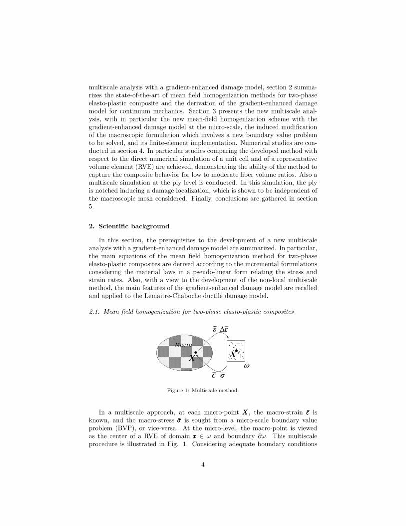
Figure 1: Multiscale method.

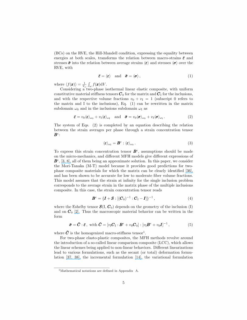
In a multiscale approach, at each macro-point XXX, the macro-strain εεε isknown, and the macro-stress σσσ is sought from a micro-scale boundary valueproblem (BVP), or vice-versa. At the micro-level, the macro-point is viewedas the center of a RVE of domain xxx ∈ ω and boundary ∂ω. This multiscaleprocedure is illustrated in Fig. 1. Considering adequate boundary conditions

4

(BCs) on the RVE, the Hill-Mandell condition, expressing the equality betweenenergies at both scales, transforms the relation between macro-strains εεε andstresses σσσ into the relation between average strains 〈εεε〉 and stresses 〈σσσ〉 over theRVE, with

εεε = 〈εεε〉 and σσσ = 〈σσσ〉 , (1)

where 〈f(xxx)〉 = 1Vω

∫ω

f(xxx)dV .Considering a two-phase isothermal linear elastic composite, with uniform

constitutive material stiffness tensors CCC0 for the matrix and CCCI for the inclusions,and with the respective volume fractions v0 + vI = 1 (subscript 0 refers tothe matrix and I to the inclusions), Eq. (1) can be rewritten in the matrixsubdomain ω0 and in the inclusions subdomain ωI as

εεε = v0〈εεε〉ω0 + vI〈εεε〉ωI and σσσ = v0〈σσσ〉ω0 + vI〈σσσ〉ωI . (2)

The system of Eqs. (2) is completed by an equation describing the relationbetween the strain averages per phase through a strain concentration tensorBBBε:

〈εεε〉ωI = BBBε : 〈εεε〉ω0 . (3)

To express this strain concentration tensor BBBε, assumptions should be madeon the micro-mechanics, and different MFH models give different expressions ofBBBε, [3, 8], all of them being an approximate solution. In this paper, we considerthe Mori-Tanaka (M-T) model because it provides good predictions for two-phase composite materials for which the matrix can be clearly identified [36],and has been shown to be accurate for low to moderate fiber volume fractions.This model assumes that the strain at infinity for the single inclusion problemcorresponds to the average strain in the matrix phase of the multiple inclusionscomposite. In this case, the strain concentration tensor reads

BBBε = III + SSS : [(CCC0)−1 : CCCI − III]−1 , (4)

where the Eshelby tensor SSS(I, CCC0) depends on the geometry of the inclusion (I)and on CCC0 [2]. Thus the macroscopic material behavior can be written in theform

σσσ = CCC : εεε , with CCC = [vICCCI : BBBε + v0CCC0] : [vIBBBε + v0III]−1 , (5)

where CCC is the homogenized macro-stiffness tensor1.For two-phase elasto-plastic composites, the MFH methods revolve around

the introduction of a so-called linear comparison composite (LCC), which allowsthe linear schemes being applied to non-linear behaviors. Different linearizationslead to various formulations, such as the secant (or total) deformation formu-lation [37, 38], the incremental formulation [14], the variational formulation

1Mathematical notations are defined in Appendix A.

5

[39–42] or the affine formulation [43, 44]. Because of its simplicity the incre-mental formulation is considered in this paper motivating a brief review of itsbasic theory.

During a finite incremental process, the constitutive equations, of the twophases, are discretized in time intervals [tn,tn+1], and the expression equivalentto (5) now relates the macroscopic homogenized stress increment ∆σσσ to themacroscopic homogenized strain increment ∆εεε through

∆σσσ = CCC : ∆εεε , (6)

where CCC is the tensor of macro-moduli of the homogenized elasto-plastic two-phase composite to be found. Toward this end, the macro linearizations of strainand stress tensors (2) are obtained from the average linearizations of strain andstress in the phases. When considering a finite increment ∆ on the time interval[tn,tn+1], these relations read

∆εεε = v0〈∆εεε〉ω0 + vI〈∆εεε〉ωI , and (7)∆σσσ = v0〈∆σσσ〉ω0 + vI〈∆σσσ〉ωI . (8)

At this point, considering the so-called linear comparison composite, the relationbetween the average incremental strains in the two phases (3) is rewritten fromthe “consistent” tangent operators CCCalg

0 of the matrix phase and CCCalgI of the

inclusions phase, leading to

〈∆εεε〉ωI = BBBε(III, CCCalg0 , CCCalg

I ) : 〈∆εεε〉ω0 . (9)

The tensor CCCalg0 (respectively CCCalg

I ) is computed from the material model ofthe matrix (respectively inclusions) phase using 〈∆εεε〉ω0 (respectively 〈∆εεε〉ωI).Thus, CCCalg

0 and CCCalgI are uniform by construction, and called comparison tan-

gent operators; Finally, similarly to the elastic counter part (5), the macroscopichomogenized stress increment ∆σσσ can be related to the macroscopic homoge-nized strain increment ∆εεε through (6) with the macro-moduli tensor of thehomogenized elasto-plastic two-phase composite evaluated from

CCC = [vICCCalgI : BBBε + v0CCC

alg0 ] : [vIBBB

ε + v0III]−1 . (10)

Note, that when computing the Eshelby tensor SSS(I, CCCiso0 ) required to compute

the Mori-Tanaka strain concentration tensor (4), only the isotropic part CCCiso0

of CCCalg0 is applied to improve prediction results. More details can be found in

reference [44].For completeness, when solving the problem at the finite element level using

a Newton-Raphson procedure, one needs to linearize the stress tensor at timetn+1 yielding

δσσσn+1 = CCCalg : δεεεn+1 , (11)

where CCCalg is the Jacobian operator obtained during the MFH process as de-scribed in section 3.1.1.

6

This method has been shown to be very accurate for 2-phase compositeswith moderate fiber volume ratios, and for which, at the RVE size, the matrixcan be considered as homogeneous isotropic and the ellipsoidal fibers can beconsidered as homogeneous transversely isotropic.

2.2. The non-local gradient modelIn order to avoid the loss of solution uniqueness and the strain localization

problem when extending MFH to damage theories, the model should be writtenin a non-local form involving gradient enrichments. Toward this end, someinternal variables a (which can be strains, accumulated plastic strain, damage...)are replaced by their weighted average a over a characteristic volume (VC) toreflect the interaction between neighboring material points [45]:

a(XXX) =1

VC

∫VC

a(yyy)φ(yyy; XXX)dV , (12)

where yyy denotes positions inside the characteristic volume VC . The weightfunction φ(yyy; XXX) determines the influence of the local internal variables in thecharacteristic volume VC on the non-local internal variable at point XXX. Forconvenience, the weight functions are assumed normalized such that one has1

VC

∫VC

φ(yyy; XXX)dV = 1.Practically, in order to avoid the direct computation of (12) in a finite ele-

ment framework, this expression can be substituted by an explicit approximatedsolution, or by an implicit form preserving the high order accuracy.

2.2.1. Explicit gradient formulationFor a sufficiently smooth field a and when taken sufficiently far from the

boundaries, the integral relation (12) can be rewritten in terms of the even-order gradients of a by expanding the field into Taylor series [27]. Odd ordersannihilate due to the symmetry of the weight functions. Neglecting terms offourth-order and higher, the integral relation (12) is approximated by the dif-ferential relation

a(XXX) = a(XXX) + l2∇2a(XXX) , (13)

where the Laplacian operator∇2a(XXX) =∑

i ∂2/∂X2i a. The internal length scale

of the non-local model is preserved in the gradient coefficient l. On top of thedifficulty of applying adequate boundary conditions, the numerical evaluationof relation (13) in a traditional finite element framework is not straightforwardas elements are usually not satisfying high order continuities. These drawbacksmotivated the development of the so-called implicit method [27].

2.2.2. Implicit gradient formulationConsidering Green functions G(yyy;XXX) as weighting functions φ(yyy; XXX) in (12),

an alternative second-order gradient approximation2 can be derived after some

2Here the approximation results from the particular choice of the weighting functions only

7

further mathematical manipulations [27], leading to

a(XXX)− l2∇2a(XXX) = a(XXX) , (14)

where the Laplacian operator is defined as ∇2a(XXX) =∑

i ∂2/∂X2i a. In contrast

to the definition (13), the non-local internal variable a is not given explicitlyin terms of a and its derivatives, but is the solution of a new boundary valueproblem consisting of the Helmholtz equation (14) completed by appropriateboundary conditions.

By opposition to the explicit form (13), this gradient model (14) is trulynon-local in the sense that variations of the local internal variable a in theneighboring of XXX always affect the non-local internal variable a(XXX), due tothe definition of the Green functions and as equation (14) is satisfied exactlyduring the computation. Another advantage of (14) compared to the explicitformulation is that it can be implemented without recourse to high-order finite-elements and that it avoids the consideration of complex boundary conditionson the non-local variable, see [27] for a complete discussion.

2.2.3. Boundary conditionsAs non-local formulations involve higher order derivatives, additional bound-

ary conditions are required to have a well-posed problem. For the implicit gra-dient model based on equation (14), the natural boundary conditions usuallyconsidered are [35]

∂a

∂n= ni

∂a

∂Xi= 0 , (15)

where nnn is the outward unit normal. Indeed, these boundary conditions lead toa behavior that is consistent with relation (12), i.e.

• a always equals a for homogeneous deformations;

• The total internal variable content is preserved in the non-local averaging:∫Ω

adΩ =∫Ω

adΩ, where Ω is the problem domain.

Note that the finite-element formulation of the implicit formulation naturallyincludes these boundary conditions, which, thus, do not need to be defined bythe user.

2.2.4. Application to the Lemaitre - Chaboche ductile damage modelIn particular, the non-local implicit approach can be applied to damage

models in order to avoid any loss of ellipticity. In this paper, we only considerthe damage in the isotropic matrix. In order to simplify the developments ofthe method, an isotropic damage model is assumed. Although to remain moregeneral, a damage variable should be represented by a fourth order tensor dueto the existence of several mechanisms of damage, this is not necessary fordamage induced by meso- or micro-plasticity [46], which justifies the use of asimple model for the matrix material. In this work, we focus on the Lemaitre -

8

Chaboche ductile damage model [46]. The damage is introduced with the usualassumption that the strain observed in the actual body and in its undamagedrepresentation are equivalent [47, 48], and the usual definition of the averageeffective stress reads

σσσ =σσσ

(1−D), (16)

where 0 ≤ D < 1 is the damage variable.Assuming an elasto-plastic material, which obeys J2 elasto-plasticity, the

von Mises stress criterion reads

f = σeq −R(p)− σY 6 0 . (17)

In this expression, f is the yield surface, σeq =√

32

dev(σσσ)1−D : dev(σσσ)

1−D is the equiv-alent von Mises effective stress, σY is the initial yield stress, R(p) > 0 is theisotropic hardening stress, and p is an internal variable characterizing the irre-versible behavior. If f < 0, the behavior remains elastic. On the other hand,if f = 0, then p is positive and the plastic strain tensor increment obeys thenormal plastic flow, which is summarized by

εεεpl = pNNN , with NNN =∂f

∂σσσ=

32

dev(σσσ)(1−D)σeq

, (18)

where NNN is the normal to the yield surface in the effective stress space. Inthis formalism, the internal variable p represents the accumulated plastic strainp = [ 23 εεε

pl : εεεpl]1/2, and, assuming small deformations, the reversible (elastic)and irreversible (plastic) strain tensors can be added (εεε = εεεel + εεεpl), yielding

σσσ = (1−D)CCCel : (εεε− εεεpl) , (19)

where CCCel is the fourth-order Hooke tensor of the sane (undamaged) material.What remains to be defined is the evolution of the damage with p. In this

paper, we focus on the Lemaitre-Chaboche ductile damage model [46]. Followingthe technique proposed in [49] to develop non-local damage laws, in this paperthe non-local accumulated plastic strain p is applied to calculate the damageevolution in the Lemaitre-Chaboche model:

D =

0, if p 6 pC ;( Y

S0)s ˙p, if p > pC .

(20)

In this expression, pC is a plastic threshold for the evolution of damage, S0 ands are the material parameters, and Y is the strain energy release rate computedas

Y =12εεεel : CCCel : εεεel . (21)

Eventually the damage can simply be obtained from the time-integration of(20): D =

∫Ddt.

9

In this gradient enhanced damage model, the non-local accumulated plasticstrain p is computed from the implicit formulation (14), which becomes

p− l2∇2p = p . (22)

In this formalism, the length scale l is related to the characteristic micro-structure length. The local accumulated plastic strain in Eq. (22) is still com-puted from the plastic flow (18). The equations governing the J2-plasticity, i.e.Eqs. (17-18) involve explicitly the local accumulated plastic strain p only, whilethe non-local form p appears in (20) only. Indeed, as demonstrated in [35, 49],considering the non-local form p in the definition of the yield surface would leadto unphysical results, such as a constant plastic strain on the whole domain.

During a finite incremental process, the constitutive equations are discretizedin time intervals [tn,tn+1], and the constitutive equations are differentiated attn+1. Remembering that for the non-local formulation the damage depends onboth εεε and on p, this linearization reads

δσσσn+1 = CCCalgD : δεεεn+1 −(

σσσ ⊗ ∂D

∂εεε

): δεεεn+1 − σσσ

∂D

∂pδpn+1 , (23)

whereCCCalgD = (1−D)CCCalg . (24)

In these last expressions, CCCalg is the derivative of the effective stress incrementwith respect to the strain increment3, [50]. Its expression, and the explicitexpressions of the damage derivatives are given in Appendix B.

3. Multiscale analysis a with gradient-enhanced damage model

The purpose of this section is to develop a multiscale model for 2-phasecomposites where the matrix material obeys an elasto-plastic behavior expe-riencing damage. Toward this end, the matrix material behavior is describedby the gradient-enhanced damage model presented in section 2.2.4. The multi-scale analysis is based on an incremental MFH scheme, as presented in section2.1, which is extended herein to account for the non-local damage model ofthe matrix. The fibers are assumed to remain elastic. As considering the im-plicit formulation of the gradient-enhanced damage model implies solving newHelmholtz-type equations, the macro-scale governing equations have to be com-pleted to fully determine the micro-macro transition. Finally the finite-elementimplementation of this MFH-based multiscale framework is derived.

3In this non-local formalism, we explicitly write the dependence of the stress in D and εεεand linearize with respect to both terms. We use symbol CCCalg for the derivative of the effectivestress increment with respect to the strain increment.

10

3.1. The gradient-enhanced damage model in the micro-scale analysisIn this section we consider a finite incremental process for which the con-

stitutive equations are discretized in time intervals [tn, tn+1]. Unless specifiedotherwise, variables are referred to their value at time tn+1 and their lineariza-tion at that time is denoted using symbol δ. The average stress and straintensors in the RVE are respectively denoted σσσ and εεε. The average micro-stressand micros-strain tensors in each phase, previously referred to as, respectively,〈σσσ〉ωi

and 〈εεε〉ωi, are now, respectively, denoted σσσi and εεεi to simplify the equa-

tions.

3.1.1. MFH with a gradient-enhanced damage modelFollowing the incremental formulation of MFH presented in section 2.1, the

stress linearization reads:

δσσσ = v0δσσσ0 + vIδσσσI . (25)

The behavior of the fibers is assumed to remain elastic, and δσσσI = CCCelI : δεεεI. The

matrix obeys the non-local damage elasto-plastic behavior described in section2.2.4, and equation (23) allows writing

δσσσ0 = CCCalgD0 : δεεε0 −

(σσσ0 ⊗

∂D

∂εεε0

): δεεε0 − σσσ0

∂D

∂pδp . (26)

However, as this last equation involves average stress and strain tensors on thematrix phase, one should be careful on the meaning of D and p which arerepresentations of, respectively, the damage and the non-local equivalent plasticstrain in the matrix of the RVE and do not correspond to the average values4.Thus, eq. (25) becomes

δσσσ = vICCCalgI : δεεεI + v0CCC

algD0 : δεεε0 − v0

(σσσ0 ⊗

∂D

∂εεε0

): δεεε0 − v0σσσ0

∂D

∂pδp , (27)

where the operators of the matrix CCCalgD0 , and of the fibers CCC

algI = CCC

elI , which

are by construction uniform, are designated as ”comparison” operators in theMFH literature.

The first two terms at the right hand side of Eq. (27) represent the stressvariation of a composite with a fictitious matrix material of uniform non-localdamage. As this non-local damage is a non-local representation of an internalvariable of the matrix only, we assume that these two terms define a LinearComparison Composite (LCC) on which the incremental Mori-Tanaka processcan be applied. Indeed, the last two terms of Eq. (27) are related to the

4Indeed, starting from σσσ = (1−D)σσσ, the average tensor 〈δσσσ〉ω0= 〈(1 − D)δσσσ〉ω0

−〈σσσδD〉ω0can be written as 〈δσσσ〉ω0

= (1−D∗) 〈δσσσ〉ω0−〈σσσ〉ω0

δD∗, where D∗ 6= 〈D〉ω0is a representation

of the damage of the matrix. For simplicity, we do not use D∗ but D in the developments ofthis section.

11

softening of the matrix due to the damage. By choice, they are not consideredwhen defining the LCC for the M-T process, and the slope (1 − D)CCCalg

0 forthe damaged matrix phase is used for two reasons. On the one hand, M-T isonly defined when the two tangent moduli of the LCC are definite positive,which would not be the case in the softening part if these two terms wereconsidered. Note that if considering another approach than the incrementalformulation, such as the affine formulation or the transformation field analysis[51, 52], this limitation could be removed. In the transformation field analysis[51, 52] for elasto-plastic composites, a relaxation stress is defined due to theirreversible behavior in the matrix. In our approach the relaxation stress, dueto plasticity and damage, is partly modeled by using the damaged elasto-plasticmodulus of matrix CCC

algD0 in the M-T process, see details here below. However,

the relaxation stress resulting from the softening in the matrix (last two terms ofEq. (27)) is omitted due to our approximation. On the other hand, neglectingthe last two terms of Eq. (27) introduces an error as the softening of the matrixdoes not lead to an unloading of fibers. However, this is an error of the sameorder of magnitude as for elasto-plastic behaviors. Indeed MFH using the LCCincremental formulation does not unload the stress in the fibers reached atthe end of the previous stress increment. This correction should result from amodification of the material stiffness. Thus we expect our M-T based MFH topredict stresses slightly above the solution obtained with a direct finite elementsimulation.

Considering a time step [tn, tn+1], the known data are the macro-totalstrain tensor εεεn, the strain increment ∆εεεn+1 and the non-local accumulatedplastic strain increment ∆pn+1 of the matrix material, as well as the internalvariables at tn. The set of non-linear equations to be solved can thus be statedas

∆εεεn+1 = v0∆εεε0n+1 + vI∆εεεIn+1 , (28)σσσn+1 = v0σσσ0n+1 + vIσσσIn+1 , (29)

∆εεεIn+1 = BBBε(III, CCCalgD0 , CCCalg

I ) : ∆εεε0n+1 , (30)

where σσσ0n+1 (respectively σσσIn+1) is evaluated from ∆εεε0n+1 and ∆pn+1 (respec-tively ∆εεεIn+1) using the non-local Lemaitre - Chaboche ductile damage modeldescribed in section 2.2.4 (respectively the elastic constitutive behavior).

Practically, this system of equations is solved using the following M-T pro-cess:

• Predict Eshelby tensor SSS(III, CCC isoD0n

) using the isotropic moduli of CCCalgD0 of

matrix at tn5.

• Initialize the strain increment in inclusions: ∆εεεn+1 → ∆εεεIn+1.

5We use CCCisoD0 evaluated at previous time step to compute the Eshelby tensor to avoid the

need of accounting for the derivation of SSS during the iteration process that follows.

12

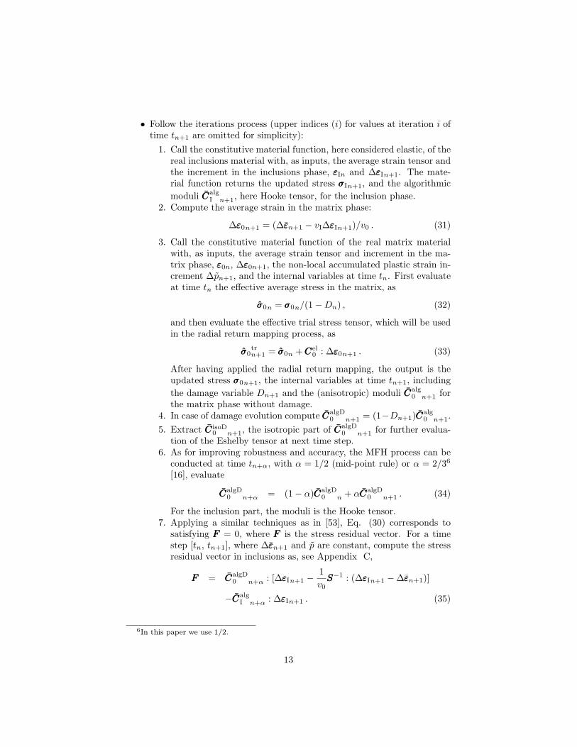
• Follow the iterations process (upper indices (i) for values at iteration i oftime tn+1 are omitted for simplicity):

1. Call the constitutive material function, here considered elastic, of thereal inclusions material with, as inputs, the average strain tensor andthe increment in the inclusions phase, εεεIn and ∆εεεIn+1. The mate-rial function returns the updated stress σσσIn+1, and the algorithmicmoduli CCCalg

I n+1, here Hooke tensor, for the inclusion phase.2. Compute the average strain in the matrix phase:

∆εεε0n+1 = (∆εεεn+1 − vI∆εεεIn+1)/v0 . (31)

3. Call the constitutive material function of the real matrix materialwith, as inputs, the average strain tensor and increment in the ma-trix phase, εεε0n, ∆εεε0n+1, the non-local accumulated plastic strain in-crement ∆pn+1, and the internal variables at time tn. First evaluateat time tn the effective average stress in the matrix, as

σσσ0n = σσσ0n/(1−Dn) , (32)

and then evaluate the effective trial stress tensor, which will be usedin the radial return mapping process, as

σσσ0trn+1 = σσσ0n + CCCel

0 : ∆εεε0n+1 . (33)

After having applied the radial return mapping, the output is theupdated stress σσσ0n+1, the internal variables at time tn+1, includingthe damage variable Dn+1 and the (anisotropic) moduli CCCalg

0 n+1 forthe matrix phase without damage.

4. In case of damage evolution compute CCCalgD0 n+1 = (1−Dn+1)CCC

alg0 n+1.

5. Extract CCC isoD0 n+1, the isotropic part of CCCalgD

0 n+1 for further evalua-tion of the Eshelby tensor at next time step.

6. As for improving robustness and accuracy, the MFH process can beconducted at time tn+α, with α = 1/2 (mid-point rule) or α = 2/36

[16], evaluate

CCCalgD0 n+α = (1− α)CCCalgD

0 n + αCCCalgD0 n+1 . (34)

For the inclusion part, the moduli is the Hooke tensor.7. Applying a similar techniques as in [53], Eq. (30) corresponds to

satisfying FFF = 0, where FFF is the stress residual vector. For a timestep [tn, tn+1], where ∆εεεn+1 and p are constant, compute the stressresidual vector in inclusions as, see Appendix C,

FFF = CCCalgD0 n+α : [∆εεεIn+1 −

1v0

SSS−1 : (∆εεεIn+1 −∆εεεn+1)]

−CCCalgI n+α : ∆εεεIn+1 . (35)

6In this paper we use 1/2.

13

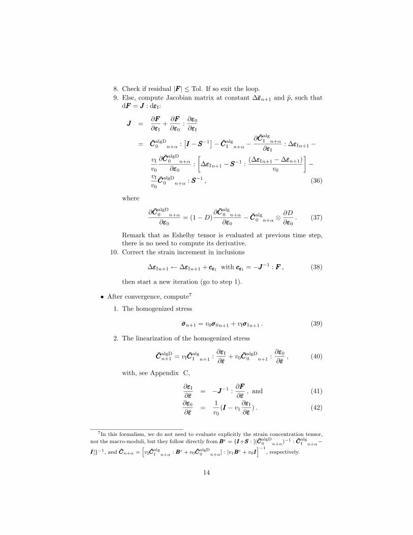
8. Check if residual |FFF | ≤ Tol. If so exit the loop.9. Else, compute Jacobian matrix at constant ∆εεεn+1 and p, such that

dFFF = JJJ : dεεεI:

JJJ =∂FFF

∂εεεI+

∂FFF

∂εεε0:

∂εεε0

∂εεεI

= CCCalgD0 n+α :

[III −SSS−1

]− CCCalg

I n+α −∂CCCalg

I n+α

∂εεεI: ∆εεεIn+1 −

vI

v0

∂CCCalgD0 n+α

∂εεε0:[∆εεεIn+1 −SSS−1 :

(∆εεεIn+1 −∆εεεn+1)v0

]−

vI

v0CCCalgD

0 n+α : SSS−1 , (36)

where

∂CCCalgD0 n+α

∂εεε0= (1−D)

∂CCCalg0 n+α

∂εεε0− CCCalg

0 n+α ⊗∂D

∂εεε0. (37)

Remark that as Eshelby tensor is evaluated at previous time step,there is no need to compute its derivative.

10. Correct the strain increment in inclusions

∆εεεIn+1 ← ∆εεεIn+1 + cccεεεI with cccεεεI = −JJJ−1 : FFF , (38)

then start a new iteration (go to step 1).

• After convergence, compute7

1. The homogenized stress

σσσn+1 = v0σσσ0n+1 + vIσσσIn+1 . (39)

2. The linearization of the homogenized stress

CCCalgDn+1 = vICCC

algI n+1 :

∂εεεI

∂εεε+ v0CCC

algD0 n+1 :

∂εεε0

∂εεε, (40)

with, see Appendix C,

∂εεεI

∂εεε= −JJJ−1 :

∂FFF

∂εεε, and (41)

∂εεε0

∂εεε=

1v0

(III − v1∂εεεI

∂εεε) . (42)

7In this formalism, we do not need to evaluate explicitly the strain concentration tensor,

nor the macro-moduli, but they follow directly from BBBε = III+SSS : [(CCCalgD0 n+α

)−1 : CCCalgI n+α

−

III]−1, and CCCn+α =hvICCC

algI n+α

: BBBε + v0CCCalgD0 n+α

] : [v1BBBε + v0IIIi−1

, respectively.

14

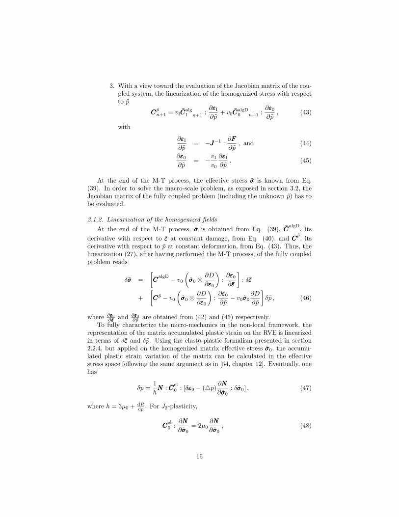
3. With a view toward the evaluation of the Jacobian matrix of the cou-pled system, the linearization of the homogenized stress with respectto p

CCC pn+1 = vICCC

algI n+1 :

∂εεεI

∂p+ v0CCC

algD0 n+1 :

∂εεε0

∂p, (43)

with

∂εεεI

∂p= −JJJ−1 :

∂FFF

∂p, and (44)

∂εεε0

∂p= −v1

v0

∂εεεI

∂p. (45)

At the end of the M-T process, the effective stress σσσ is known from Eq.(39). In order to solve the macro-scale problem, as exposed in section 3.2, theJacobian matrix of the fully coupled problem (including the unknown p) has tobe evaluated.

3.1.2. Linearization of the homogenized fieldsAt the end of the M-T process, σσσ is obtained from Eq. (39), CCC

algD, itsderivative with respect to εεε at constant damage, from Eq. (40), and CCC

p, itsderivative with respect to p at constant deformation, from Eq. (43). Thus, thelinearization (27), after having performed the M-T process, of the fully coupledproblem reads

δσσσ =[CCC

algD − v0

(σσσ0 ⊗

∂D

∂εεε0

):

∂εεε0

∂εεε

]: δεεε

+[CCC p − v0

(σσσ0 ⊗

∂D

∂εεε0

):

∂εεε0

∂p− v0σσσ0

∂D

∂p

]δp , (46)

where ∂εεε0∂εεε and ∂εεε0

∂p are obtained from (42) and (45) respectively.To fully characterize the micro-mechanics in the non-local framework, the

representation of the matrix accumulated plastic strain on the RVE is linearizedin terms of δεεε and δp. Using the elasto-plastic formalism presented in section2.2.4, but applied on the homogenized matrix effective stress σσσ0, the accumu-lated plastic strain variation of the matrix can be calculated in the effectivestress space following the same argument as in [54, chapter 12]. Eventually, onehas

δp =1hNNN : CCC

el0 : [δεεε0 − (4p)

∂NNN

∂σσσ0: δσσσ0] , (47)

where h = 3µ0 + dRdp . For J2-plasticity,

CCCel0 :

∂NNN

∂σσσ0= 2µ0

∂NNN

∂σσσ0, (48)

15

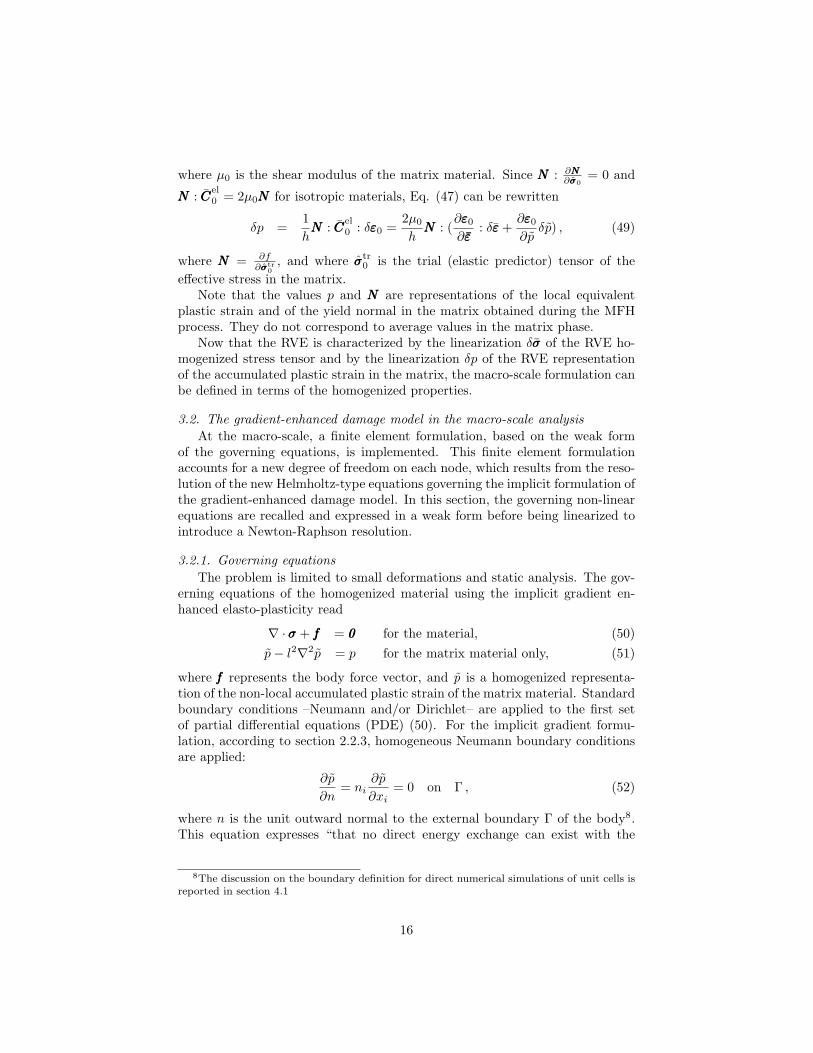
where µ0 is the shear modulus of the matrix material. Since NNN : ∂NNN∂σσσ0

= 0 and

NNN : CCCel0 = 2µ0NNN for isotropic materials, Eq. (47) can be rewritten

δp =1hNNN : CCC

el0 : δεεε0 =

2µ0

hNNN : (

∂εεε0

∂εεε: δεεε +

∂εεε0

∂pδp) , (49)

where NNN = ∂f∂σσσtr

0, and where σσσtr

0 is the trial (elastic predictor) tensor of theeffective stress in the matrix.

Note that the values p and NNN are representations of the local equivalentplastic strain and of the yield normal in the matrix obtained during the MFHprocess. They do not correspond to average values in the matrix phase.

Now that the RVE is characterized by the linearization δσσσ of the RVE ho-mogenized stress tensor and by the linearization δp of the RVE representationof the accumulated plastic strain in the matrix, the macro-scale formulation canbe defined in terms of the homogenized properties.

3.2. The gradient-enhanced damage model in the macro-scale analysisAt the macro-scale, a finite element formulation, based on the weak form

of the governing equations, is implemented. This finite element formulationaccounts for a new degree of freedom on each node, which results from the reso-lution of the new Helmholtz-type equations governing the implicit formulation ofthe gradient-enhanced damage model. In this section, the governing non-linearequations are recalled and expressed in a weak form before being linearized tointroduce a Newton-Raphson resolution.

3.2.1. Governing equationsThe problem is limited to small deformations and static analysis. The gov-

erning equations of the homogenized material using the implicit gradient en-hanced elasto-plasticity read

∇ · σσσ + fff = 000 for the material, (50)p− l2∇2p = p for the matrix material only, (51)

where fff represents the body force vector, and p is a homogenized representa-tion of the non-local accumulated plastic strain of the matrix material. Standardboundary conditions –Neumann and/or Dirichlet– are applied to the first setof partial differential equations (PDE) (50). For the implicit gradient formu-lation, according to section 2.2.3, homogeneous Neumann boundary conditionsare applied:

∂p

∂n= ni

∂p

∂xi= 0 on Γ , (52)

where n is the unit outward normal to the external boundary Γ of the body8.This equation expresses “that no direct energy exchange can exist with the

8The discussion on the boundary definition for direct numerical simulations of unit cells isreported in section 4.1

16

surroundings of the body and ensures that the net dissipation in the bodyvanishes for constant damage” [55]

However, as it will be shown in the next section, this boundary conditionwill be accounted for when establishing the finite-element formulation, and willnot have to be enforced explicitly during the computation.

3.2.2. Weak formulationWeak form of the set of Eqs. (50-51) is established using suitable weight

functions defined in the n + 1 − dimensional spaces:wwwu ∈ [C 0]n The weight function of the displacement field,wp ∈ [C 0] The weight function of non-local accumulated plastic

strain of the matrix material.Multiplying equilibrium condition (50) with the displacement weight func-

tion wwwu and integrating the result over the domain Ω yields∫Ω

wwwu · [∇ · σσσ + fff ]dΩ = 0 . (53)

Applying the divergence theorem, the natural boundary conditions for the bound-ary traction vector (σσσ·nnn = TTT ) on ΓT , the essential boundary conditions on Γ−ΓT

and the symmetry property of the stress tensor leads to∫Ω

[Owwwu ]T : σσσdΩ =∫

Ω

wwwu · fffdΩ +∫

ΓT

wwwu · TTTdΓ . (54)

The same method is used to treat the second PDE (51), which results in:∫Ω

(wp p + l2Owp · Op)dΩ =∫

Ω

wppdΩ , (55)

where (52) has been used. Note that as the boundary conditions (52) havealready been considered herein, they will not have to be explicitly applied inthe finite element formulation.

3.2.3. LinearizationConsidering a time step [tn, tn+1], it is assumed that the non-linear system

(54-55) has been solved at time tn. The problem is stated as solving the followingequations at time tn+1:∫

Ω

[Owwwu ]T : σσσn+1dΩ =∫

Ω

wwwu · fffn+1dΩ +∫

ΓT

wwwu · TTTn+1dΓ , (56)∫Ω

(wp pn+1 + l2Owp · Opn+1)dΩ =∫

Ω

wppn+1dΩ . (57)

The set of non-linear equations (56-57) can be recast in the following form:

Ψ(σσσ, p)|tn+1 = 0 , (58)

17

which is solved using the Newton-Raphson method. Thus, at each iteration i oftime step [tn, tn+1], we have

Ψ(σσσin+1, p

in+1) +

∂Ψ∂(σσσ, p)

∣∣∣σσσi

n+1,pin+1

[(σσσi+1n+1, p

i+1n+1)− (σσσi

n+1, pin+1)] = 0 . (59)

Using Eqs. (56- 57), the explicit form of Eq. (59) can be expressed as∫Ω

[Owwwu ]T : δσσσi+1n+1dΩ =∫

Ω

wwwu · fffn+1dΩ +∫

ΓT

wwwu · TTTn+1dΓ−∫

Ω

[Owwwu ]T : σσσin+1dΩ , (60)

and

−∫

Ω

wpδpi+1n+1dΩ +

∫Ω

[wpδpi+1n+1 + l2∇wp · ∇(δpi+1

n+1)]dΩ =∫Ω

wppin+1dΩ−

∫Ω

[wp pin+1 + l2∇wp · ∇pi

n+1]dΩ . (61)

According to the classical resolution schemes, the key issue of solving theweak form (60-61) is to find the expressions of δσσσi+1

n+1 and δpi+1n+1 in terms of

δεεεi+1n+1 and δpi+1

n+1, which results from Eqs. (46) and (49). The resolution cannow be achieved using a classical finite-element (FE) formulation.

3.3. Finite element implementation - Discretization and incremental-iterativeformulation

After substituting Eqs. (46) and (49) into the linearized weak form (60-61), the finite element discretization is straightforwardly formulated using theGalerkin approach. Toward this end, the displacement field UUU and the non-localaccumulated plastic strain field p can be interpolated in each element Ωe usingtraditional shape function matrices NNNu and NNN p as follows:

UUU = NNNuuuu, and p = NNN pppp , (62)

where the vectors uuu and ppp contain the assembled nodal values of the displace-ments and of the non-local accumulated plastic strain field, respectively. Simi-larly, the weight functions are interpolated using the same shape functions

wwwu = NNNudududu, and wp = NNN pdddppp , (63)

where dududu and dddppp are arbitrary values fulfilling the essential boundary conditions.The macro-strain tensorial field and the gradient field of the non-local accu-

mulated plastic strain can easily be deduced, in terms of the problem unknowns,from

εεε = BBBuuuu, and ∇p = ∇NNN pppp = BBBpppp , (64)

18

where BBBu and BBBp represent the matrix strain operator and the matrix operatorfor the non-local accumulated plastic strain, respectively. Therefore, using Eq.(63), and the arbitrary nature of dududu and dddppp, the linearized weak form (60-61)can be stated in the following matrix form at iteration ’i’ of time step [tn, tn+1]:[

KKKiuu KKKi

up

KKKipu KKKi

pp

] [δuuuδp

]=

[FFFn+1

ext −FFF iint

FFF ip −FFF i

p

], (65)

with the sub-matrices defined by

KKKiuu =

∫Ω

BBBTuCCC

iDBBBudΩ , (66a)

KKKiup =

∫Ω

BBBTuSDSDSD

iNNN pdΩ , (66b)

KKKipu = −

∫Ω

NNNTp SpSpSp

iBBBudΩ , and (66c)

KKKipp =

∫Ω

[(1− Sip)NNN

Tp NNN p + l2BBBT

p BBBp]dΩ . (66d)

In these last expressions, CCCiD, SDSDSD

i, SpSpSpi and Si

p are the matrix representations

[54, appendix C] of the previously defined tensors [CCCalgD − v0

(σσσ0 ⊗ ∂D

∂εεε0

):

∂εεε0∂εεε ]

∣∣∣i, [CCC p − v0

(σσσ0 ⊗ ∂D

∂εεε0

): ∂εεε0

∂p − v0σσσ0∂D∂p ]

∣∣∣i, 2µ0

hi NNN i : ∂εεε0∂εεε

∣∣∣i

and 2µ0hi NNN i :

∂εεε0∂p

∣∣∣irespectively. Finally the force vectors are easily obtained from

FFFn+1ext =

∫Ω

NNNTufffn+1dΩ +

∫ΓT

NNNTuTTTn+1dΓ , (67a)

FFF iint =

∫Ω

BBBTu σσσidΩ , (67b)

FFF ip =

∫Ω

NNNTp pppidΩ , and (67c)

FFF ip =

∫Ω

(NNNTp NNN p + l2BBBT

p BBBp)pppidΩ . (67d)

4. Numerical simulations

The new gradient enhanced MFH model described in section 3 has beenimplemented as a non-linear FE module in GMSH [56]. Two kinds of locking-free elements have been used. On the one hand linear hexahedra with selectedreduced integration, and on the other hand, quadratic tetrahedra with 4 Gausspoints. The same polynomial order is used for the different fields. Although themethod could also be used with 2D elements, only the most general 3D formu-lation is implemented. The numerical verification of the model is first carriedout by comparing the results obtained from the homogenized law to the re-sults obtained from direct numerical simulations on unit cells for different fibers

19

percentages. As the MFH process implemented uses the non-local Lemaitre -Chaboche ductile damage model described in section 2.2.4, this non-local modelis equally available for the direct numerical simulations of the composite. Af-terward, the gradient enhanced MFH model is applied to simulate the responseof a notched sample under transverse loading.

4.1. Numerical verificationsIn this section, the gradient enhanced MFH model is used to compute the ef-

fective response of unidirectional fiber reinforced elasto-plastic composites. Theconsidered composites consist in a continuous elasto-plastic matrix, experienc-ing damage, reinforced by unidirectional continuous fibers with linear elasticbehavior. As an example, the matrix considered is made of epoxy and thereinforcements are continuous carbon fibers.

4.1.1. Tests descriptionThe properties of the matrix are: Young’s modulus E0 = 2.89 GPa, Poisson’s

ratio ν0 = 0.3 and yielding stress σY = 35.0 MPa. The hardening law of theepoxy material follows an exponential law

R(p) = h0[1− e−mp] , (68)

where h0 = 73.0 MPa and m = 60. The damage law obeys Eq. (20), with theparameters S0 = 2.0 MPa, s = 0.5 and pC = 0.0, which are reference values forthe unidirectional carbon fiber reinforced epoxy [46]. By lack of data for epoxymatrix, we consider these composite damage values for the matrix.

The carbon fibers are linear elastic, with EI = 238 GPa and νI = 0.26.Moreover, the carbon fibers are assumed to be isotropic, which is far from beingtrue9, to enhance the difference of material properties in the transverse directionand, thus, to illustrate the ability of the method to perform the homogenization.Results obtained will thus not match experimental results but will allow to verifythe new MFH process developed.

Reference results are provided by finite element computations performed onunit cells where the micro-structure is fully meshed. In these unit cells, it isassumed that the matrix and the fibers can be considered as homogeneous mate-rials. As these simulations involve softening, the representativeness of the unitcells is disputable as a shear band of comparable size of the volume appears[33, 34, 57–59]. This requires particular attention, as using averaging methods[59], proscribing periodic boundary conditions but applying adequate boundaryconditions [33, 34], when extracting the macroscopic behavior from the cell sim-ulations, particularly when performing a computational homogenization. How-ever, such methods are beyond the scope of this paper whose main purpose isthe development of a MFH method, for which the RVE remains conceptual.

With the non-local model, the Helmholtz equation (51) has to be solvedin the domain of interest with the associate boundary conditions (52) on its

9The Young modulus of fibers in transverse direction is lower than in longitudinal direction.

20

(a) Periodic unit cell (b) Random unit cell

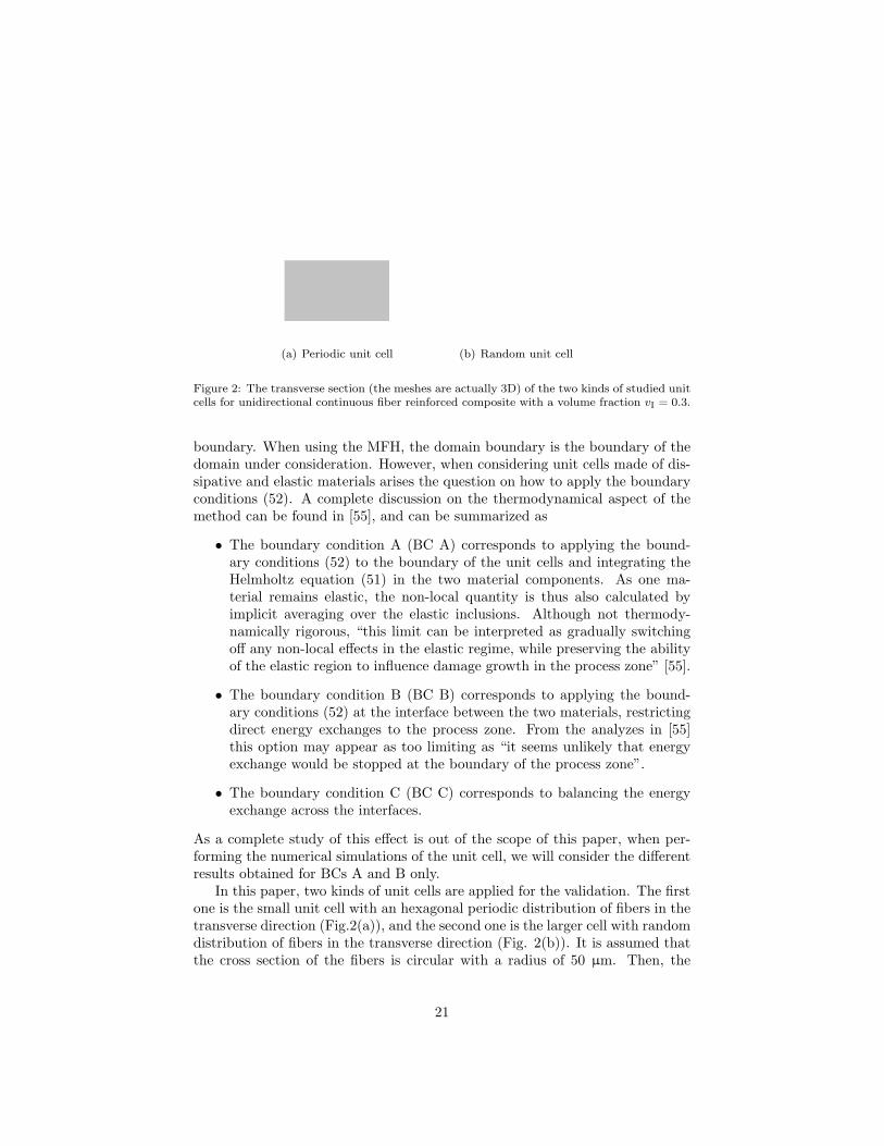
Figure 2: The transverse section (the meshes are actually 3D) of the two kinds of studied unitcells for unidirectional continuous fiber reinforced composite with a volume fraction vI = 0.3.

boundary. When using the MFH, the domain boundary is the boundary of thedomain under consideration. However, when considering unit cells made of dis-sipative and elastic materials arises the question on how to apply the boundaryconditions (52). A complete discussion on the thermodynamical aspect of themethod can be found in [55], and can be summarized as

• The boundary condition A (BC A) corresponds to applying the bound-ary conditions (52) to the boundary of the unit cells and integrating theHelmholtz equation (51) in the two material components. As one ma-terial remains elastic, the non-local quantity is thus also calculated byimplicit averaging over the elastic inclusions. Although not thermody-namically rigorous, “this limit can be interpreted as gradually switchingoff any non-local effects in the elastic regime, while preserving the abilityof the elastic region to influence damage growth in the process zone” [55].

• The boundary condition B (BC B) corresponds to applying the bound-ary conditions (52) at the interface between the two materials, restrictingdirect energy exchanges to the process zone. From the analyzes in [55]this option may appear as too limiting as “it seems unlikely that energyexchange would be stopped at the boundary of the process zone”.

• The boundary condition C (BC C) corresponds to balancing the energyexchange across the interfaces.

As a complete study of this effect is out of the scope of this paper, when per-forming the numerical simulations of the unit cell, we will consider the differentresults obtained for BCs A and B only.

In this paper, two kinds of unit cells are applied for the validation. The firstone is the small unit cell with an hexagonal periodic distribution of fibers in thetransverse direction (Fig.2(a)), and the second one is the larger cell with randomdistribution of fibers in the transverse direction (Fig. 2(b)). It is assumed thatthe cross section of the fibers is circular with a radius of 50 µm. Then, the

21

size of the unit cell can be calculated according to the fiber volume fractionvI and the number of fibers considered in the simulation [60]. In the secondcase, as the size of the unit cell is not much larger than the micro-structurelength (only four fibers per cell are considered), six different occurrences, withrandom fiber distributions are simultaneously considered in order to capturethe scattering effect due to the violation of the length scale separation. Aswe choose traction-free/displacement-controlled boundary conditions, the cellwith only four fibers allows obtaining results close to the periodic cell results, asshown in the following part. The periodic cells have about 250 linear hexahedralelements, while the non-periodic unit cells have about 2500 quadratic tetrahedralelements, which allows to reach mesh convergence10. All the meshes have onelayer of elements on the thickness. The comparisons between simulations aresuccessively achieved for 15, 30 and 50 % volume fractions of fibers. For theperiodic cells, BCs A and B are considered, while for the random distributioncells, only the BCs A are considered.

The characteristic length of the non-local model in the simulations of unitcells should be related to the width of the shear band in the matrix material.The size of the unit cells is about a few hundreds micro-meters, which is muchsmaller than the characteristic length of the matrix material, and the interac-tions between the matrix material points are blocked off by the elastic fibers.Therefore, the simulations on unit cells are not sensitive to reasonable valuesof l. As only a simple tensile test is considered, the MFH simulation will giveuniform numerical results, which are not affected by the value of l. So we setl2 = 2.0 mm2, which is a typical value for composite [49].

4.1.2. ResultsFirst, a loading-unloading cycle is applied in the direction transverse to

the fibers. A maximal deformation of 10 % is reached before the unloadingproceeds to zero-transverse deformation. Boundary conditions correspond touniform displacements11, with controlled deformation in the loading direction,traction-free condition in the other transverse direction and plane-strain con-dition in the longitudinal direction. The plane-strain condition in the fibersdirection correspond to the state of a composite ply, while the combination oftraction-free, strain-controlled displacements in the transverse directions givesgood convergence results in terms of unit-cell size.

The effective behaviors predicted by the MFH models and the FE resultsfor the three fiber volume ratios are presented in Fig. 3. For the three fibervolume ratios, the homogenized property is dominated by the properties ofthe matrix, with an obvious elasto-plastic behavior exhibiting softening. Whenconsidering the periodic cells, BC B predicts higher softening than BC A, as it

10Number of elements is not exactly the same for all the fiber volume fractions nor for allthe realizations of the unit cells

11For the periodic unit cells and the MFH problems, this corresponds to periodic boundaryconditions by symmetry.

22

-150

-100

-50

0

50

100

150

200

0 0.02 0.04 0.06 0.08 0.1

Strain

Stre

ss (M

Pa)

Random Cells, BC APeriodical Cell, BC APeriodical Cell, BC BMFH

(a) vI = 0.15

-150

-100

-50

0

50

100

150

200

0 0.02 0.04 0.06 0.08 0.1

Strain

Stre

ss (M

Pa)

Random Cells, BC APeriodical Cell, BC APeriodical Cell, BC BMFH

(b) vI = 0.30

-150

-100

-50

0

50

100

150

200

0 0.02 0.04 0.06 0.08 0.1

Strain

Stre

ss (M

Pa)

Random Cells, BC A

Periodical Cell, BC A

Periodical Cell, BC B

MFH

(c) vI = 0.50

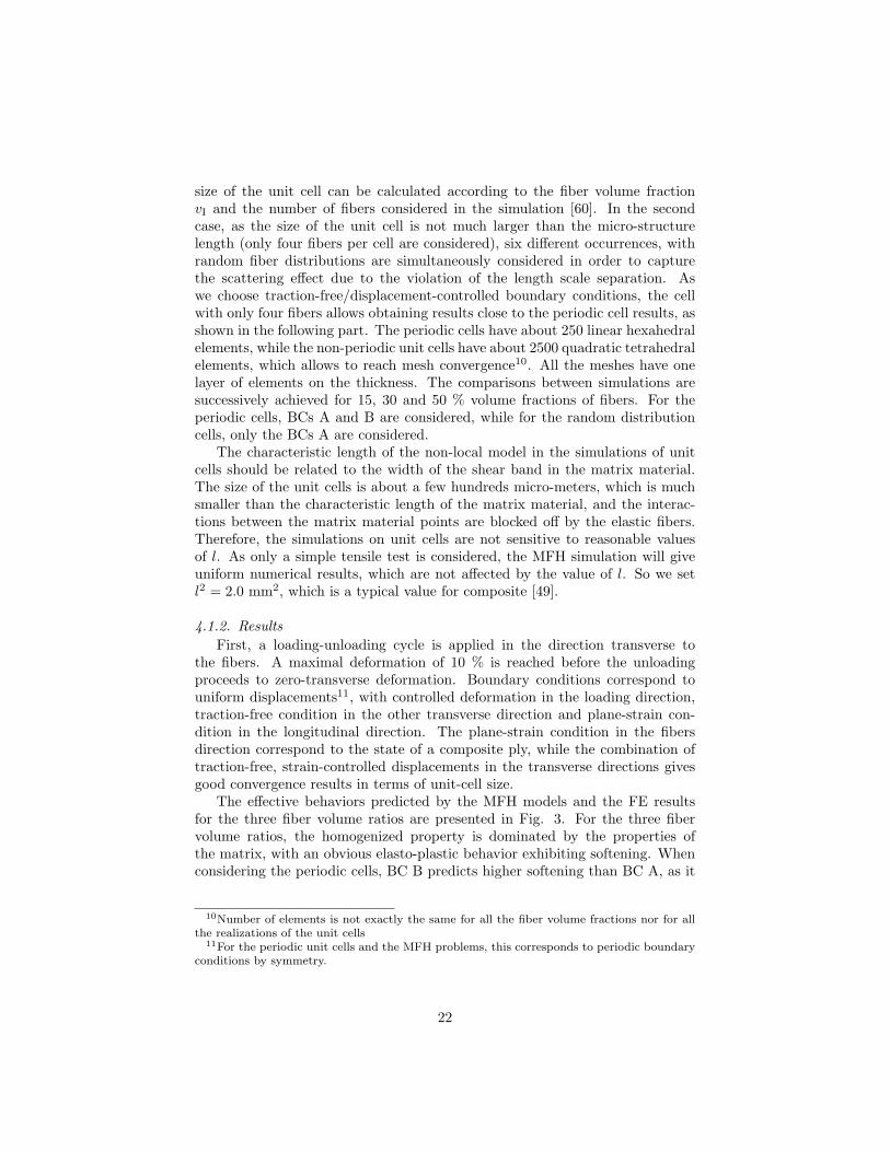
Figure 3: Stress-strain behavior of the epoxy fiber reinforced composite, for different fibervolume ratios, under transverse loading.

was expected since matrix constraints are lower. However, for low to moderate(up to 30 % fiber volume ratio), the difference remains reduced. The 6 randomcell occurrences converged as they exhibit a solution similar to the periodic unitcell, although the statistical dispersion increases with the fiber volume ratio.For the fiber volume fractions of vI = 15% and 30%, rather good predictionsare given by the MFH model, with, as expected, higher macroscopic stressand damage predicted by the MFH due to the incremental LCC formulation.However for vI = 50%, the MFH model overestimates the macroscopic stresscompared to the periodic unit cell results. This error comes from the assumptionof Mori - Tanaka based MFH, which can give an accurate prediction when thevolume fraction of inclusions is lower than 30%. Also, for the computations ofrandom cells of vI = 50%, only three random cells reach the end of the loading-unloading cycle. This might be due to the abrupt increase of damage, which canreach 1.0 in high stress concentration area before the maximum loading stageis reached. More explanations for this will be given in the next section. Notethat these curves are for comparison purpose as few composites will sustain thislevel of deformation.

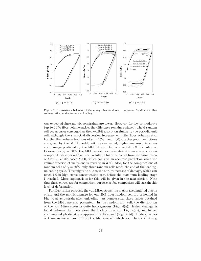
For illustration purpose, the von Mises stress, the matrix accumulated plasticstrain and the matrix damage for one 30% fiber random cell are presented inFig. 4 at zero-strain after unloading. As comparison, those values obtainedfrom the MFH are also presented. In the random unit cell, the distributionof the von Mises stress is quite homogeneous (Fig. 4(a)), higher damage isfound between the fibers along the loading direction (Fig. 4(c)), and higheraccumulated plastic strain appears in a 45o-band (Fig. 4(b)). Highest valuesof those in matrix are seen at the fiber/matrix interfaces. On the contrary,

23

0 1.1e+8 2.2e+8 σeq

(a) Von Mises stress (Pa)

0 0.47 0.939 p

(b) Local accumulated plas-tic strain

0 0.12 0.24 Damage

(c) Damage

0 6.09e+7 1.22e+8σeq

(d) Von Mises stress (Pa)

0 0.092 0.184p

(e) Local accumulated plas-tic strain

0 0.10 0.20Damage

(f) Damage

Figure 4: The von Mises stress, accumulated plastic strain in the matrix phase and damagein the matrix phase at zero-strain after unloading and plastic compression, for a 30% fibersrandom unit cell (a)∼(c), and those of a 30% fiber homogenized cell (d)∼(f) under transverseloading. The scale for the von Mises stress shows the maximal value reached during theloading process.

uniform values of the von Mises stress, accumulated plastic strain and damageare obtained by the cell with the MFH process (Fig. 4(d)-Fig. 4(f)). This wasexpected, but as the homogenized material exhibits softening, it is importantto make sure localization problems are avoided under uniform loading, which isthe case in this formulation.

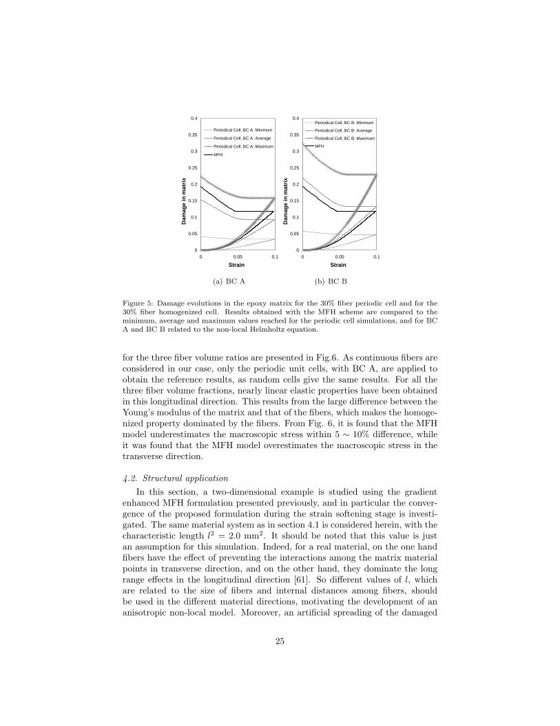
The constant non-local damage in the matrix obtained with the MFH schemeis compared, in Fig. 5, to the minimum, average, and maximal values reachedin the epoxy matrix for the periodic cell simulations, for 30 % fiber volumefraction. For the periodic cells, the effect of the boundary conditions consideredfor the Helmholtz equation is studied. From this figure, it can be seen thatthe damage in the periodic cell has a higher average value when applying BCB, as expected. The non-local MFH damage remains in-between the averageand (minimal) maximal value of the matrix, for BC A (B), respectively. Thisconfirms that the damage predicted by the MFH is a good image of the averagevalue in the matrix.

Next, loading along the fiber direction is studied. Boundary conditions cor-respond to uniform displacements, with controlled deformation in the loadingdirection, traction-free and plane-strain conditions in the two transverse direc-tions. The effective behaviors predicted by the MFH models and the FE results

24

0

0.05

0.1

0.15

0.2

0.25

0.3

0.35

0.4

0 0.05 0.1

Strain

Dam

age

in m

atrix

Periodical Cell, BC A: Minimum

Periodical Cell, BC A: Average

Periodical Cell, BC A: Maximum

MFH

(a) BC A

0

0.05

0.1

0.15

0.2

0.25

0.3

0.35

0.4

0 0.05 0.1

Strain

Dam

age

in m

atrix

Periodical Cell, BC B: Minimum

Periodical Cell, BC B: Average

Periodical Cell, BC B: Maximum

MFH

(b) BC B

Figure 5: Damage evolutions in the epoxy matrix for the 30% fiber periodic cell and for the30% fiber homogenized cell. Results obtained with the MFH scheme are compared to theminimum, average and maximum values reached for the periodic cell simulations, and for BCA and BC B related to the non-local Helmholtz equation.

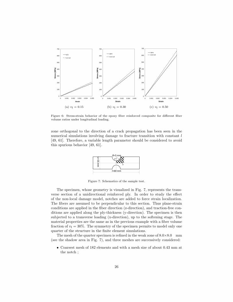
for the three fiber volume ratios are presented in Fig.6. As continuous fibers areconsidered in our case, only the periodic unit cells, with BC A, are applied toobtain the reference results, as random cells give the same results. For all thethree fiber volume fractions, nearly linear elastic properties have been obtainedin this longitudinal direction. This results from the large difference between theYoung’s modulus of the matrix and that of the fibers, which makes the homoge-nized property dominated by the fibers. From Fig. 6, it is found that the MFHmodel underestimates the macroscopic stress within 5 ∼ 10% difference, whileit was found that the MFH model overestimates the macroscopic stress in thetransverse direction.

4.2. Structural applicationIn this section, a two-dimensional example is studied using the gradient

enhanced MFH formulation presented previously, and in particular the conver-gence of the proposed formulation during the strain softening stage is investi-gated. The same material system as in section 4.1 is considered herein, with thecharacteristic length l2 = 2.0 mm2. It should be noted that this value is justan assumption for this simulation. Indeed, for a real material, on the one handfibers have the effect of preventing the interactions among the matrix materialpoints in transverse direction, and on the other hand, they dominate the longrange effects in the longitudinal direction [61]. So different values of l, whichare related to the size of fibers and internal distances among fibers, shouldbe used in the different material directions, motivating the development of ananisotropic non-local model. Moreover, an artificial spreading of the damaged

25

0

100

200

300

400

500

600

700

0 0.001 0.002 0.003 0.004 0.005

Strain

Stre

ss (M

Pa)

MFH

Unit Cell

(a) vI = 0.15

0

100

200

300

400

500

600

700

0 0.001 0.002 0.003 0.004 0.005

Strain

Stre

ss (M

Pa)

MFH

Unit Cell

(b) vI = 0.30

0

100

200

300

400

500

600

700

0 0.001 0.002 0.003 0.004 0.005

Strain

Stre

ss (M

Pa)

MFHUnit Cell

(c) vI = 0.50

Figure 6: Stress-strain behavior of the epoxy fiber reinforced composite for different fibervolume ratios under longitudinal loading.

zone orthogonal to the direction of a crack propagation has been seen in thenumerical simulations involving damage to fracture transition with constant l[49, 61]. Therefore, a variable length parameter should be considered to avoidthis spurious behavior [49, 61].

l=60 mm

w=16 m

m

R=5 mm

x

y

Figure 7: Schematics of the sample test.

The specimen, whose geometry is visualized in Fig. 7, represents the trans-verse section of a unidirectional reinforced ply. In order to study the effectof the non-local damage model, notches are added to force strain localization.The fibers are assumed to be perpendicular to this section. Thus plane-strainconditions are applied in the fiber direction (z-direction), and traction-free con-ditions are applied along the ply-thickness (y-direction). The specimen is thensubjected to a transverse loading (x-direction), up to the softening stage. Thematerial properties are the same as in the previous example with a fiber volumefraction of vI = 30%. The symmetry of the specimen permits to model only onequarter of the structure in the finite element simulations.

The mesh of the quarter specimen is refined in the weak zone of 8.0×8.0 mm(see the shadow area in Fig. 7), and three meshes are successively considered:

• Coarsest mesh of 182 elements and with a mesh size of about 0.43 mm atthe notch ;

26

• Intermediate mesh of 360 elements and with a mesh size of about 0.3 mmat the notch;

• Finest mesh of 1120 elements and with a the mesh size of about 0.15 mmat the notch.

0

50

100

150

200

250

300

0 0.5 1Displacement (mm)

Forc

e (N

/mm

)

Mesh size 0.43 mm

Mesh size: 0.3 mm

Mesh size: 0.15 mm

Figure 8: Force per unit ply length vs. displacement of the sample for different meshes.

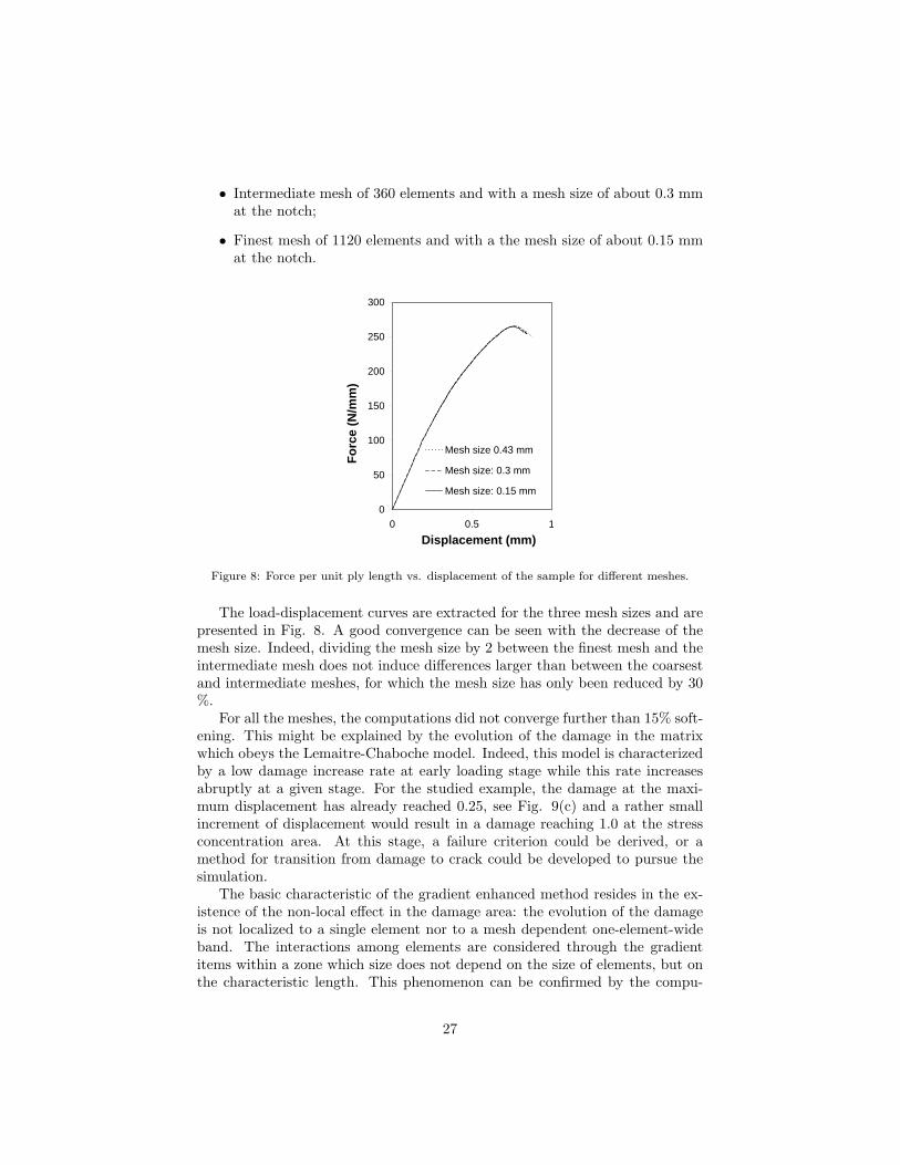
The load-displacement curves are extracted for the three mesh sizes and arepresented in Fig. 8. A good convergence can be seen with the decrease of themesh size. Indeed, dividing the mesh size by 2 between the finest mesh and theintermediate mesh does not induce differences larger than between the coarsestand intermediate meshes, for which the mesh size has only been reduced by 30%.

For all the meshes, the computations did not converge further than 15% soft-ening. This might be explained by the evolution of the damage in the matrixwhich obeys the Lemaitre-Chaboche model. Indeed, this model is characterizedby a low damage increase rate at early loading stage while this rate increasesabruptly at a given stage. For the studied example, the damage at the maxi-mum displacement has already reached 0.25, see Fig. 9(c) and a rather smallincrement of displacement would result in a damage reaching 1.0 at the stressconcentration area. At this stage, a failure criterion could be derived, or amethod for transition from damage to crack could be developed to pursue thesimulation.

The basic characteristic of the gradient enhanced method resides in the ex-istence of the non-local effect in the damage area: the evolution of the damageis not localized to a single element nor to a mesh dependent one-element-wideband. The interactions among elements are considered through the gradientitems within a zone which size does not depend on the size of elements, but onthe characteristic length. This phenomenon can be confirmed by the compu-

27

0 6.03e+07 1.2e+08σeq

(a) Von Mises stress (Pa)

0 0.205 0.41 p

(b) Local accumulated plas-tic strain

0 0.125 0.25Damage

(c) Damage

0 6.03e+07 1.2e+08 σeq

(d) Von Mises stress (Pa)

0 0.205 0.41 p

(e) Local accumulated plas-tic strain

0 0.125 0.25Damage

(f) Damage

0 6.03e+07 1.2e+08σeq

(g) Von Mises stress (Pa)

0 0.205 0.41 p

(h) Local accumulated plas-tic strain

0 0.125 0.25Damage

(i) Damage

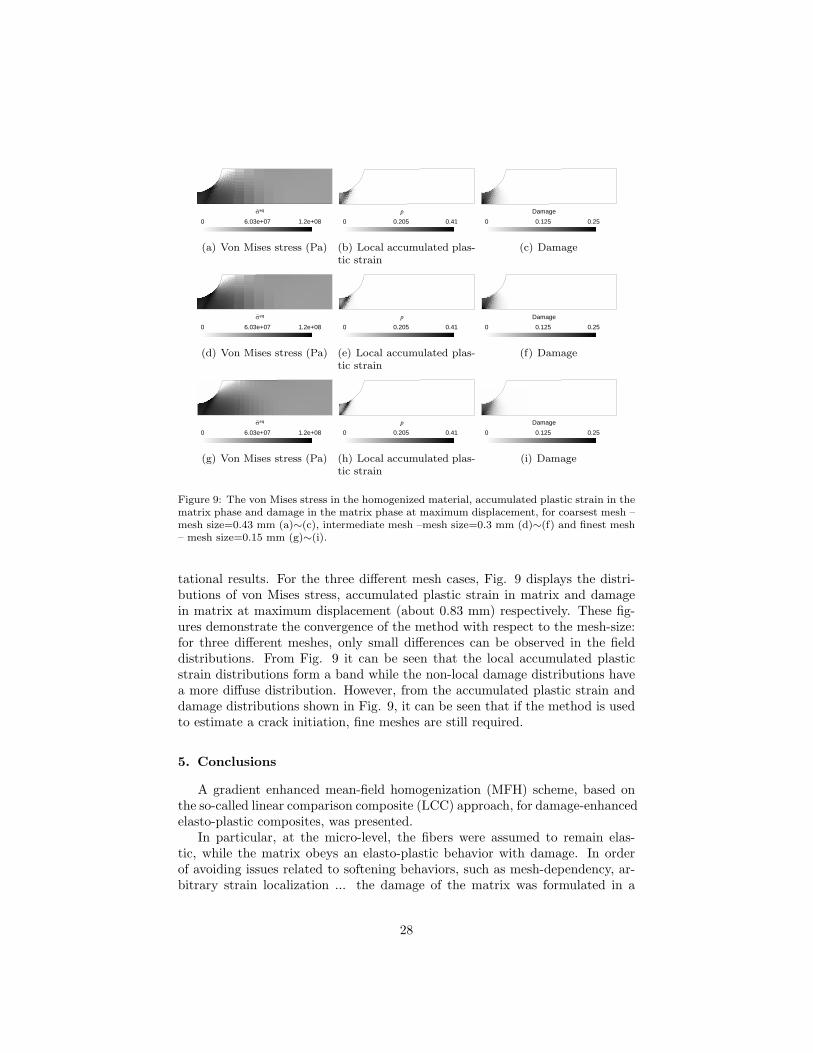
Figure 9: The von Mises stress in the homogenized material, accumulated plastic strain in thematrix phase and damage in the matrix phase at maximum displacement, for coarsest mesh –mesh size=0.43 mm (a)∼(c), intermediate mesh –mesh size=0.3 mm (d)∼(f) and finest mesh– mesh size=0.15 mm (g)∼(i).

tational results. For the three different mesh cases, Fig. 9 displays the distri-butions of von Mises stress, accumulated plastic strain in matrix and damagein matrix at maximum displacement (about 0.83 mm) respectively. These fig-ures demonstrate the convergence of the method with respect to the mesh-size:for three different meshes, only small differences can be observed in the fielddistributions. From Fig. 9 it can be seen that the local accumulated plasticstrain distributions form a band while the non-local damage distributions havea more diffuse distribution. However, from the accumulated plastic strain anddamage distributions shown in Fig. 9, it can be seen that if the method is usedto estimate a crack initiation, fine meshes are still required.

5. Conclusions

A gradient enhanced mean-field homogenization (MFH) scheme, based onthe so-called linear comparison composite (LCC) approach, for damage-enhancedelasto-plastic composites, was presented.

In particular, at the micro-level, the fibers were assumed to remain elas-tic, while the matrix obeys an elasto-plastic behavior with damage. In orderof avoiding issues related to softening behaviors, such as mesh-dependency, ar-bitrary strain localization ... the damage of the matrix was formulated in a

28

non-local way, using the so-called implicit approach. In this approach, the dam-age is computed from a non-local equivalent accumulated plastic strain, whichis obtained by solving new Helmholtz-type equations relating the non-local ac-cumulated plastic strain to its local expression.

At the homogenized macro-level, the resulting formulation required four de-grees of freedom per nodes, the three usual displacement unknowns, and a newdegree of freedom, which is a representation of the equivalent accumulated plas-tic strain in the matrix. Thus, the set of traditional mechanical equations wascompleted in a fully coupled way by a new set of equations corresponding tothe weak formulation of the non-local implicit formulation.

Although general, this approach was applied to unidirectional carbon-fiber,epoxy-matrix composites. First the responses under uniform strain obtainedwith the new non-local MFH formulation were compared to the responses ob-tained with the direct numerical simulation of periodical cells and RVEs. Towardthis end, a loading/unloading cycle was applied in the transverse direction. Forlow fiber volume ratios (< 30 %) results are in excellent agreement, includingduring the softening and unloading parts of the loading history. For averagefiber volume ratios (up to 50 %), the method is less accurate (error up to ∼20 %), which is mainly explained by the M-T assumption and the incrementalMFH approach adopted in this paper. Indeed MFH using the LCC incrementalformulation does not correct the previous stress increments from a modificationof the material stiffness, due to the plastic or damage behavior.

Finally the methodology was applied to study the transverse loading of anotched composite ply. In particular it was shown that the method can capturethe softening and lead to results that converge with mesh refinement, demon-strating the ability of the method to be used to compute mesoscopic or macro-scopic structures.

Nevertheless, the method was found to remain accurate for moderate fibervolume ratios only. The MFH could thus be enriched by second statisticalmoments [18] to improve the accuracy. Adding anisotropic behaviors in the fiberand/or in the damage law and in the characteristic length, as well as consideringfiber debonding would allow to compare predictions with experimental resultsas more physical inputs would be accounted for. Also, in a future work themodel will be used to predict macro-crack initiation, including comparisons toexperimental results.

Appendix A. Tensorial operations and notations

• Dots and colons are used to indicate tensor products contracted over oneand two indices respectively:

uuu · vvv = uivi, (aaa · uuu)i = aijuj ;(aaa · bbb)ij = aikbkj , aaa : bbb = aijbji ;

(CCC : aaa)ij = Cijklalk, (CCC : DDD)ijkl = CijmnDnmkl . (A.1)

29

• Dyadic products are designated by ⊗:

(uuu⊗ vvv)ij = uivj , (aaa⊗ bbb)ijkl = aijbkl . (A.2)

• Symbols 111 and III designate the second- and fourth-order symmetric identitytensors respectively:

111ij = δij , IIIijkl =12(δikδjl + δilδjk) , (A.3)

where δij = 1 if i = j, δij = 0 if i 6= j.

• The spherical and deviatoric operators are IIIvol and IIIdev respectively:

IIIvol ≡ 13111⊗ 111, IIIdev = III − IIIvol , (A.4)

so that for symmetric tensors aij = aji we have:

IIIvol : aaa =13amm111 , IIIdev : aaa = aaa− 1

3amm111 = dev(aaa) . (A.5)

• Any fourth-order tensors CCC and DDD define the following scalar invariant:

CCC :: DDD = CijklDlkji = DDD :: CCC (A.6)

Using this definition, the following results are easily obtained:

IIIvol :: IIIvol = 1, IIIdev :: IIIdev = 5 and IIIvol :: IIIdev = 0 . (A.7)

• Any symmetric and isotropic fourth-order tensor CCC iso is a linear combina-tion of IIIvol and IIIdev, and can be written as follows

CCC iso = (IIIvol :: CCC iso)IIIvol +15(IIIdev :: CCC iso)IIIdev (A.8)

Appendix B. The Lemaitre-Chaboche ductile damage model in non-local form

In this section, subscript 0 related to the matrix material is omitted forsimplicity.

In the ”time-continuum” formulation of sec. 2.2.4, a ”continuum” elasto-plastic tangent operator such that ˙σσσ = CCCep : εεε can be calculated from (e.g. [54,chapter 12]):

CCCep = CCCel − (2µ)2

hNNN ⊗NNN, h = 3µ +

dR

dp> 0 , (B.1)

where µ is the shear modulus. Due to the finite increments of strain and stressbetween time tn and time tn+1, the operator CCCalg = ∂∆σσσ

∂∆εεε differs from CCCep,

30

[50]. In the case of the radial return mapping assumption, the derivative of theeffective stress increment with respect to the strain increment reads (e.g. [54,chapter 12])

CCCalg = CCCep − (2µ)2(∆p)σeq

σeq, tr

∂NNN

∂σσσ, with

∂NNN

∂σσσ=

1σeq

(32IIIdev −NNN ⊗NNN) . (B.2)

In this last relation, σeq, tr is the trial (elastic predictor) value of σeq, and ∆p isthe accumulated plastic strain increment in the time interval. Note that in caseof plastic flow both CCCep and CCCalg are anisotropic, and that in case of elasticityCCCalg reduces to CCCel.

The increment of damage in one time step is expressed as [46]:

∆D = (Yn+α

S0)s∆p , (B.3)

where

Y =12εεεe : CCCel

0 : εεεe and Yn+α = (1− α)Yn + αYn+1 . (B.4)

It can be easily deduced that

∂Y

∂εεεe:

∂εεεe

∂εεε: δεεε = αεεεe : CCCalg : δεεε , (B.5)

leading to

δD(εεε, p) ≈ ∂∆D

∂Y

∂Y

∂εεεe:

∂εεεe

∂εεε: δεεε +

∂∆D

∂pδp

= s∆p(Yn+α)s−1

Ss0

∂Y

∂εεεe:

∂εεεe

∂εεε: δεεε + (

Yn+α

S0)sδp

= αs∆p(Yn+α)s−1

Ss0

εεεe : CCCalg : δεεε + (Yn+α

S0)sδp . (B.6)

Appendix C. Stress residual vector

The equation to be satisfied at the end of the MFH procedure is Eq. (30).Multiplying Eq. (28) by BBBε(III, CCCalgD

0 n+α, CCCalgI n+α) ans using (30) lead to

v0∆εεεIn+1 + vIBBBε(III, CCCalgD

0 n+α, CCCalgI n+α) : ∆εεεIn+1 =

BBBε(III, CCCalgD0 n+α, CCCalg

I n+α) : ∆εεεn+1 . (C.1)

With the M-T assumption the strain concentration tensor follows from (4), andEq. (C.1) reads

∆εεεIn+1 + v0SSS : [(CCCalgD0 n+α)−1 : CCCalg

I n+α − III] : ∆εεεIn+1 = ∆εεεn+1 , (C.2)

31

or again FFF = 0 with

FFF = CCCalgD0 n+α : [∆εεεIn+1 −

1v0

SSS−1 : (∆εεεIn+1 −∆εεεn+1)]

−CCCalgI n+α : ∆εεεIn+1 . (C.3)

In order to satisfy FFF = 0, Eq. (C.3) is linearized as

dFFF =∂FFF

∂εεεI: d∆εεεI +

∂FFF

∂εεε0: d∆εεε0 +

∂FFF

∆εεε: d∆εεε +

∂FFF

∂pdp . (C.4)

When solving FFF = 0 at constant ∆εεε and constant p, as v0∆εεε0 + vI∆εεεI isalso constant, the iteration process relies on dFFF = JJJ : dεεεI with

JJJ =∂FFF

∂εεεI+

∂FFF

∂εεε0:

∂εεε0

∂εεεI

= CCCalgD0 n+α :

[III −SSS−1

]− CCCalg

I n+α −∂CCCalg

I n+α

∂εεεI: ∆εεεIn+1 −

vI

v0

∂CCCalgD0 n+α

∂εεε0:[∆εεεIn+1 −SSS−1 :

(∆εεεIn+1 −∆εεεn+1)v0

]−

vI

v0CCCalgD

0 n+α : SSS−1 . (C.5)

Once FFF = 0 is satisfied, the effect on the strain increment in each phase of avariation d∆εεε at constant ∆p can directly be obtained by constraining dFFF = 0,and Eq. (C.4) leads to

0 =∂FFF

∂εεεI: d∆εεεI +

∂FFF

∂εεε0: d∆εεε0 +

∂FFF

∂εεε: d∆εεε , (C.6)

or again

∂εεεI

∂εεε= −JJJ−1 :

∂FFF

∂εεε. (C.7)

As under these circumstances dεεε = v0dεεε0+vIdεεεI, this last equation is completedby

∂εεε0

∂εεε=

1v0

(III − v1∂εεεI

∂εεε) . (C.8)

The same relations can be obtained for a linearization with respect to p atconstant ∆εεε.

Acknowledgment

The research has been funded by the Walloon Region under the agreementSIMUCOMP no 1017232 (CT-EUC 2010-10-12) in the context of the ERA-NET+, Matera + framework.

32

References

[1] P. Kanoute, D. Boso, J. Chaboche, B. Schrefler, Multiscale Methods forComposites: A Review, Archives of Computational Methods in Engineering16 (2009) 31–75, ISSN 1134-3060, 10.1007/s11831-008-9028-8.

[2] J. D. Eshelby, The Determination of the Elastic Field of an EllipsoidalInclusion, and Related Problems, Proceedings of the Royal Society of Lon-don. Series A, Mathematical and Physical Sciences 241 (1226) (1957) pp.376–396, ISSN 00804630.

[3] T. Mori, K. Tanaka, Average stress in matrix and average elastic energyof materials with misfitting inclusions, Acta Metallurgica 21 (5) (1973)571–574, cited By (since 1996) 1814.

[4] Y. Benveniste, A new approach to the application of Mori-Tanaka’s theoryin composite materials, Mechanics of Materials 6 (2) (1987) 147 – 157, ISSN0167-6636, doi:DOI: 10.1016/0167-6636(87)90005-6.

[5] B. Budiansky, On the elastic moduli of some heterogeneous materials, Jour-nal of the Mechanics and Physics of Solids 13 (4) (1965) 223 – 227, ISSN0022-5096, doi:DOI: 10.1016/0022-5096(65)90011-6.

[6] E. Kroner, Berechnung der elastischen Konstanten des Vielkristalls aus denKonstanten des Einkristalls, Zeitschrift fur Physik A Hadrons and Nuclei151 (1958) 504–518, ISSN 0939-7922, 10.1007/BF01337948.

[7] A. Hershey, The elasticity of an isotropic aggregate of anisotropic cubiccrystals, Journal of Applied mechanics-transactions of the ASME 21 (3)(1954) 236–240.

[8] R. Hill, A self-consistent mechanics of composite materials, Journal of theMechanics and Physics of Solids 13 (4) (1965) 213 – 222, ISSN 0022-5096,doi:DOI: 10.1016/0022-5096(65)90010-4.

[9] D. R. S. Talbot, J. R. Willis, Variational Principles for Inhomogeneous Non-linear Media, IMA Journal of Applied Mathematics 35 (1) (1985) 39–54,doi:10.1093/imamat/35.1.39.

[10] D. R. S. Talbot, J. R. Willis, Bounds and Self-Consistent Estimates forthe Overall Properties of Nonlinear Composites, IMA Journal of AppliedMathematics 39 (3) (1987) 215–240, doi:10.1093/imamat/39.3.215.

[11] P. Ponte Castaneda, The effective mechanical properties of nonlinearisotropic composites, Journal of the Mechanics and Physics of Solids 39 (1)(1991) 45–71, ISSN 0022-5096, doi:DOI: 10.1016/0022-5096(91)90030-R.

[12] P. Ponte Castaneda, A New Variational Principle and its Application toNonlinear Heterogeneous Systems, SIAM Journal on Applied Mathematics52 (5) (1992) 1321–1341, ISSN 00361399.

33

[13] D. Talbot, J. Willis, Some simple explicit bounds for the overall behaviourof nonlinear composites, International Journal of Solids and Structures29 (14-15) (1992) 1981 – 1987, ISSN 0020-7683, doi:DOI: 10.1016/0020-7683(92)90188-Y.

[14] R. Hill, Continuum micro-mechanics of elastoplastic polycrystals, Journalof the Mechanics and Physics of Solids 13 (2) (1965) 89 – 101, ISSN 0022-5096, doi:DOI: 10.1016/0022-5096(65)90023-2.

[15] H. E. Pettermann, A. F. Plankensteiner, H. J. Bohm, F. G. Rammerstorfer,A thermo-elasto-plastic constitutive law for inhomogeneous materials basedon an incremental Mori-Tanaka approach, Computers & Structures 71 (2)(1999) 197 – 214, ISSN 0045-7949, doi:DOI: 10.1016/S0045-7949(98)00208-9.

[16] I. Doghri, A. Ouaar, Homogenization of two-phase elasto-plastic compos-ite materials and structures: Study of tangent operators, cyclic plastic-ity and numerical algorithms, International Journal of Solids and Struc-tures 40 (7) (2003) 1681 – 1712, ISSN 0020-7683, doi:DOI: 10.1016/S0020-7683(03)00013-1.

[17] J. Chaboche, P. Kanoute, A. Roos, On the capabilities of mean-field ap-proaches for the description of plasticity in metal matrix composites, Inter-national Journal of Plasticity 21 (7) (2005) 1409 – 1434, ISSN 0749-6419,doi:DOI: 10.1016/j.ijplas.2004.07.001.

[18] I. Doghri, L. Brassart, L. Adam, J. S. Gerard, A second-moment incremen-tal formulation for the mean-field homogenization of elasto-plastic com-posites, International Journal of Plasticity 27 (3) (2011) 352 – 371, ISSN0749-6419, doi:DOI: 10.1016/j.ijplas.2010.06.004.

[19] V. Kouznetsova, M. G. D. Geers, W. A. M. Brekelmans, Multi-scale con-stitutive modelling of heterogeneous materials with a gradient-enhancedcomputational homogenization scheme, International Journal for Numeri-cal Methods in Engineering 54 (8) (2002) 1235–1260.

[20] V. Kouznetsova, M. Geers, W. Brekelmans, Multi-scale second-order com-putational homogenization of multi-phase materials: a nested finite el-ement solution strategy, Computer Methods in Applied Mechanics andEngineering 193 (48-51) (2004) 5525 – 5550, ISSN 0045-7825, doi:DOI:10.1016/j.cma.2003.12.073, advances in Computational Plasticity.

[21] R. De Borst, Simulation of strain localization: a reappraisal of the Cosseratcontinuum, Engineering Computations 8 (4) (1991) 317 – 332, ISSN 0264-4401.

[22] Z. P. Bazant, T. B. Belytchko, T. P. Chang, Continuum Theory for Strain-Softening, Journal of Engineering Mechanics-ASCE 110 (12) (1984) 1666–1692, doi:10.1061/(ASCE)0733-9399(1984)110:12(1666).

34

[23] H. M. Zbib, E. C. Aifantis, A Gradient-Dependent Flow Theory of Plastic-ity: Application to Metal and Soil Instabilities, Applied Mechanics Reviews42 (11S) (1989) S295–S304, doi:10.1115/1.3152403.

[24] R. De Borst, L. Sluys, H.-B. Muhlhaus, J. Pamin, Fundamental issues infinite element analyses of localization of deformation, Engineering Compu-tations 10 (2) (1993) 99 – 121, ISSN 0264-4401.

[25] M. Geers, Experimental Analysis and Computational Modelling of Damageand Fracture, Ph.D. thesis, University of Technology, Eindhoven (Nether-lands)., 1997.

[26] R. Peerlings, R. de Borst, W. Brekelmans, M. Geers, Gradient-enhanceddamage modelling of concrete fracture, Mech. Cohesive-Frictional Mat. 3(1998) 323–342.

[27] R. Peerlings, R. de Borst, W. Brekelmans, J. de Vree, Gradient-enhanceddamage for quasi-brittle materials, Int. J. Numer. Meth. Engng 39 (1996)3391–3403.

[28] X. Liu, G. Hu, A continuum micromechanical theory of overall plas-ticity for particulate composites including particle size effect, Interna-tional Journal of Plasticity 21 (4) (2005) 777 – 799, ISSN 0749-6419, doi:10.1016/j.ijplas.2004.04.014.

[29] C. Dascalu, A two-scale damage model with material length, ComptesRendus Mecanique 337 (9-10) (2009) 645 – 652, ISSN 1631-0721, doi:10.1016/j.crme.2009.09.008.

[30] R. Knockaert, I. Doghri, Nonlocal constitutive models with gradients ofinternal variables derived from a micro/macro homogenization procedure,Computer Methods in Applied Mechanics and Engineering 174 (1-2) (1999)121 – 136, ISSN 0045-7825, doi:DOI: 10.1016/S0045-7825(98)00282-5.

[31] T. Massart, R. Peerlings, M. Geers, A dissipation-based control method forthe multi-scale modelling of quasi-brittle materials, C. R. Mecanique 333(2005) 521527.

[32] T. Massart, R. Peerlings, M. Geers, An enhanced multi-scale approach formasonry wall computations, Int. J. Numer. Meth. Engng 69 (5) (2007)1022–1059.

[33] E. Coenen, V. Kouznetsova, M. Geers, Enabling microstructure-based dam-age and localization analyses and upscaling, Modelling and Simulation inMaterials Science and Engineering 19 (7) (2011) 074008.

[34] E. Coenen, V. Kouznetsova, M. Geers, Novel boundary conditions forstrain localization analyses in microstructural volume elements, Interna-tional Journal for Numerical Methods in Engineering .

35

[35] R. Peerlings, M. Geers, R. de Borst, W. Brekelmans, A critical compar-ison of nonlocal and gradient-enhanced softening continua, Int. J. SolidsStructures 38 (2001) 7723–7746.

[36] J. Segurado, J. Llorca, A numerical approximation to the elastic propertiesof sphere-reinforced composites, Journal of the Mechanics and Physics ofSolids 50 (10) (2002) 2107 – 2121, ISSN 0022-5096.

[37] M. Berveiller, A. Zaoui, An extension of the self-consistent scheme toplastically-flowing polycrystals, Journal of the Mechanics and Physics ofSolids 26 (5-6) (1978) 325 – 344, ISSN 0022-5096, doi:DOI: 10.1016/0022-5096(78)90003-0.

[38] G. J. Weng, The overall elastoplastic stress-strain relations of dual-phasemetals, Journal of the Mechanics and Physics of Solids 38 (3) (1990) 419 –441, ISSN 0022-5096, doi:DOI: 10.1016/0022-5096(90)90007-Q.

[39] P. Ponte Castaneda, Exact second-order estimates for the effective mechan-ical properties of nonlinear composite materials, Journal of the Mechanicsand Physics of Solids 44 (6) (1996) 827 – 862, ISSN 0022-5096, doi:DOI:10.1016/0022-5096(96)00015-4.

[40] L. Brassart, L. Stainier, I. Doghri, L. Delannay, A variational formulationfor the incremental homogenization of elasto-plastic composites, Journalof the Mechanics and Physics of Solids 59 (12) (2011) 2455 – 2475, ISSN0022-5096, doi:10.1016/j.jmps.2011.09.004.

[41] N. Lahellec, P. Suquet, On the effective behavior of nonlinear inelasticcomposites: I. Incremental variational principles, Journal of the Mechanicsand Physics of Solids 55 (9) (2007) 1932 – 1963, ISSN 0022-5096, doi:10.1016/j.jmps.2007.02.003.

[42] N. Lahellec, P. Ponte Castaneda, P. Suquet, Variational estimates for theeffective response and field statistics in thermoelastic composites with intra-phase property fluctuations, Proceedings of the Royal Society A: Mathe-matical, Physical and Engineering Science 467 (2132) (2011) 2224–2246,doi:10.1098/rspa.2010.0609.

[43] R. Masson, M. Bornert, P. Suquet, A. Zaoui, An affine formulation for theprediction of the effective properties of nonlinear composites and polycrys-tals, Journal of The Mechanics and Physics of Solids 48 (2000) 1203–1227,doi:10.1016/S0022-5096(99)00071-X.

[44] O. Pierard, I. Doghri, Study of Various Estimates of the Macroscopic Tan-gent Operator in the Incremental Homogenization of Elastoplastic Com-posites, International Journal for Multiscale Computational Engineering4 (4) (2006) 521–543, ISSN 1543-1649.

36

[45] Z. P. Bazant, G. Pijaudier-Cabot, Nonlocal Continuum Dam-age, Localization Instability and Convergence, Journal of AppliedMechanics 55 (2) (1988) 287–293, doi:10.1115/1.3173674, URLhttp://link.aip.org/link/?AMJ/55/287/1.

[46] J. Lemaitre, R. Desmorat, Engineering damage mechanics: ductile, creep,fatigue and brittle failures, Springer-Verlag, Berlin, ISBN 3540215034,2005.

[47] J. Lemaitre, Coupled elasto-plasticity and damage constitutive equations,Computer Methods in Applied Mechanics and Engineering 51 (1-3) (1985)31 – 49, ISSN 0045-7825, doi:DOI: 10.1016/0045-7825(85)90026-X.

[48] I. Doghri, Numerical implementation and analysis of a class of metal plas-ticity models coupled with ductile damage, International Journal for Nu-merical Methods in Engineering 38 (20) (1995) 3403–3431, ISSN 1097-0207,doi:10.1002/nme.1620382004.

[49] M. G. D. Geers, R. de Borst, W. A. M. Brekelmans, R. H. J. Peerlings,Strain-based transient-gradient damage model for failure analyses, Com-puter methods in applied mechanics and engineering 160 (1998) 133–153.

[50] J. C. Simo, R. L. Taylor, Consistent tangent operators for rate-independentelastoplasticity, Computer Methods in Applied Mechanics and Engineer-ing 48 (1) (1985) 101 – 118, ISSN 0045-7825, doi:DOI: 10.1016/0045-7825(85)90070-2.

[51] G. J. Dvorak, Transformation Field Analysis of Inelastic Composite Mate-rials, Proceedings: Mathematical and Physical Sciences 437 (1900) (1992)311–327.

[52] G. J. Dvorak, Y. A. Bahei-El-Din, A. M. Wafa, Implementation of thetransformation field analysis for inelastic composite materials, Computa-tional Mechanics 14 (3) (1994) 201–228.

[53] L. Brassart, Homogenization of elasto-(visco)plastic composites: history-dependent incremental and variational approaches, Ph.D. thesis, The Uni-versit catholique de Louvain, Louvain-la-Neuve (Belgium)., 2011.

[54] I. Doghri, Mechanics of Deformable Solids- Linear, Nonlinear, Analyticaland Computational Aspects, Springer-Verlag, Berlin, ISBN 3540669604,2000.

[55] R. Peerlings, T. Massart, M. Geers, A thermodynamically mo-tivated implicit gradient damage framework and its applica-tion to brick masonry cracking, Computer Methods in Ap-plied Mechanics and Engineering 193 (30) (2004) 3403 –3417, ISSN 0045-7825, doi:10.1016/j.cma.2003.10.021, URLhttp://www.sciencedirect.com/science/article/pii/S0045782504001380.

37

[56] C. Geuzaine, J.-F. Remacle, Gmsh: A 3-D finite element mesh genera-tor with built-in pre- and post-processing facilities, International Journalfor Numerical Methods in Engineering 79 (11) (2009) 1309–1331, URLhttp://dx.doi.org/10.1002/nme.2579.

[57] I. Gitman, H. Askes, L. Sluys, Representative volume: Existence andsize determination, Engineering Fracture Mechanics 74 (16) (2007)2518 – 2534, ISSN 0013-7944, doi:10.1016/j.engfracmech.2006.12.021, URLhttp://www.sciencedirect.com/science/article/pii/S0013794406004772.

[58] C. Pelissou, J. Baccou, Y. Monerie, F. Perales, Determination of thesize of the representative volume element for random quasi-brittle com-posites, International Journal of Solids and Structures 46 (14-15) (2009)2842 – 2855, ISSN 0020-7683, doi:10.1016/j.ijsolstr.2009.03.015, URLhttp://www.sciencedirect.com/science/article/pii/S0020768309001334.

[59] V. P. Nguyen, O. Lloberas-Valls, M. Stroeven, L. J. n. Sluys, Onthe existence of representative volumes for softening quasi-brittlematerials – A failure zone averaging scheme, Computer Meth-ods in Applied Mechanics and Engineering 199 (45-48) (2010)3028 – 3038, ISSN 0045-7825, doi:10.1016/j.cma.2010.06.018, URLhttp://www.sciencedirect.com/science/article/pii/S0045782510001854.

[60] C. Gonzalez, J. LLorca, Multiscale modeling of fracture in fiber-reinforcedcomposites, Acta Materialia 54 (16) (2006) 4171 – 4181, ISSN 1359-6454.

[61] M. Geers, R. de Borst, W. Brekelmans, R. Peerlings, Validation and inter-nal length scale determination for a gradient damage model: application toshort glass-fibre-reinforced polypropylene, International Journal of Solidsand Structures 36 (17) (1999) 2557 – 2583, ISSN 0020-7683.

38