A Multiresolution Strategy for Numerical Homogenization ofNonlinear ODEsG. Beylkin�Program in Applied MathematicsUniversity of Colorado at BoulderBoulder, CO 80309-0526 M. E. BrewsteryBattelle Paci�c Northwest LaboratoriesP.O. Box 999Richland, WA 99352A. C. GilbertzDepartment of MathematicsPrinceton UniversityPrinceton, NJ 08544October 28, 1997I IntroductionThere are many di�cult, interesting, and important problems which incorporate multiple scales and whichare prohibitively expensive to solve on the �nest scales. In many problems of this kind it is su�cient to�nd the solution on a coarse scale only. However, we cannot disregard the �ne scale contributions as thebehavior of the solution on the coarse scale is a�ected by the �ne scales. In these problems it is necessaryto obtain a procedure for constructing the equations on a coarse scale that account for the contributionsfrom these scales. This amounts to writing an e�ective equation for the coarse scale component of thesolution which can be solved more economically. Alternatively, we might want to construct simpler �ne scaleequations whose solutions have the same coarse properties as the solutions of more complicated systems.These simpler equations would also be considerably less expensive to solve. These procedures are generallyreferred to as homogenization, though the speci�cs of the approaches vary signi�cantly.An example of a problem which encompasses many scales and which is di�cult to solve on the �nestscale is molecular dynamics. The highest frequency motion of a polymer chain under the fully coupled setof Newton's equations determines the largest stable integration time step for the system. In the contextof long time dynamics the high frequency motions of the system are not of interest but current numerical�The research was partially supported by ARPA grant F49620-93-1-0474 and ONR grant N00014-91-J4037.yThe research was partially supported by ARPA grant F49620-93-1-0474.zThe research was partially supported by AT&T Ph.D. Fellowship Program and Associated Western Universities.1

methods (see [1],[17]) which directly access the low frequency motions of the polymer are ad hoc methods,not methods which take into account the e�ects of the high frequency behavior. The work of Bornemannand Sch�utte (see [16],[6]) is a notable exception and appears quite promising.Let us brie y mention several classical approaches to homogenization. The classical theory of homogeniza-tion, developed in part by Bensoussan, Lions, and Papanicolaou [3]; Jikov, Kozlov, and Oleinik [12]; Murat[15]; and Tartar[18], poses the problem as follows: Given a family of di�erential operators L�, indexed by aparameter �, assume that the boundary value problemL�u� = f in (with u� subject to the appropriate boundary conditions) is well-posed in a Sobolev space H for all � andthat the solutions u� form a bounded subset of H so that there is a weak limit u0 in H of the solutions u�.The small parameter � might represent the relative magnitude of the �ne and coarse scales. The problemof homogenization is to �nd the di�erential equation that u0 satis�es and to construct the correspondingdi�erential operator. We call the homogenized operator L0 and the equation L0u0 = f in the homogenizedequation.There are several methods for solving this problem. A standard technique is to expand the solution inpowers of �, to substitute the asymptotic series into the di�erential equations and associated boundaryconditions, and then to recursively solve for the coe�cients of the series given the �rst order approximationto the solution (see [14], [2], and [13] for more details). If we consider a probabilistic interpretation of thesolutions to elliptic or parabolic PDEs as averages of functionals of the trajectory of a di�usion process,then homogenization involves the weak limits of probability measures de�ned by a stochastic process ([3]).In [12] and [3], the methods of asymptotic expansions and of G-convergence are used to examine familiesof operators L�. Murat and Tartar (see [15] and [18]) developed the method of compensated compactness.Coifman et al (see [8]) have recently shown that there are intrinsic links between compensated compactnesstheory and the tools of classical harmonic analysis (such as Hardy spaces and operator estimates).Using a multiresolution approach, Beylkin and Brewster in [7] give a procedure for constructing an equationdirectly for the coarse scale component of the solution. This process is called reduction. From this e�ectiveequation one can determine a simpler equation for the original function with the same coarse scale behavior.Unlike the asymptotic approach for traditional homogenization, the reduction procedure in [7] consists of areduction operator which takes an equation at one scale and constructs the e�ective equation at an adjacentscale (the next coarsest scale). This reduction operator can be used recursively provided that the form ofthe equation is preserved under the transition. For systems of linear ordinary di�erential equations a stepof the multiresolution reduction procedure consists of changing the coordinate system to split variables intoaverages and di�erences (in fact, quite literally in the case of the Haar basis), expressing the di�erencesin terms of the averages, and eliminating the di�erences from the equations. For systems of linear ODEsthere are relatively simple explicit expressions for the coe�cients of the resulting reduced system. Becausethe system is organized so that the form of the equations is preserved, we may apply the reduction step2

recursively to obtain the reduced system over several scales.M. Dorobantu in [9] and A. Gilbert in [10] apply the technique of MRA homogenization to the one-dimensional elliptic problem and derive results which relate the MRA approach to classical homogenizationtheory. A multiresolution approach to the reduction of elliptic PDEs and eigenvalue problems has beendeveloped in [5]. It is shown in [5] that by choosing an appropriate MRA for a given problem, the smalleigenvalues of the reduced operator di�er only slightly from those of the original operator.In this paper we consider a multiresolution strategy for the reduction and homogenization of nonlinearequations; in particular, of a small system of nonlinear ordinary di�erential equations. The main di�cultyin performing a reduction step in the nonlinear case as compared to the linear case is that there are noexplicit expressions for the di�erences in terms of the averages. We o�er two basic approaches to addressthis problem. First, it appears possible not to require an analytic substitution for the di�erences and, instead,to rely on a numerical procedure. Second, we use a series expansion of the nonlinear functions in terms ofa small parameter related to the discretization at a given scale (e.g., the step size of the discretization) andobtain analytic recurrence relations for the terms of the expansion. These recurrence relations allow us toreduce repeatedly. A third method is a hybrid of the two basic approaches.In the �rst section we present a derivation of the reduction procedure for nonlinear ODEs and the seriesexpansion of the recurrence relations. In the second section we discuss the implementation of the approachesto reduction. We discuss the homogenization procedure for nonlinear equations in the �nal section. We leavedetailed discussions of the results to the appendices.

3

II MRA Reduction MethodsII.1 Linear Reduction MethodLet us brie y review the reduction method for linear systems of di�erential equations presented in [7].Consider the di�erential equationddt�G(t)x(t) + q(t)� = F (t)x(t) + p(t); t 2 [0; 1];where F and G are bounded matrix-valued functions and p and q are vector-valued functions (with elementsin L2([0; 1])). We will rewrite this di�erential equation as an integral equationG(t)x(t) + q(t)� � = Z t0 �F (s)x(s) + p(s)� ds; t 2 [0; 1]; (2.1)(where � is a complex or real vector) since we can preserve the form of this equation under reduction, whilewe cannot preserve the form of the corresponding di�erential equation. To express this integral equationin terms of an operator equation on functions in L2([0; 1]), let F and G be the operators whose actions onfunctions are pointwise multiplication by F and G and let K be the integral operator whose kernel K isK(s; t) = � 1; 0 � s � t0; otherwise:Then equation (2.1) can be rewritten as Gx+ q � � =K(Fx+ p):We will use a general MRA of L2([0; 1]) in this discussion. See Appendix B for de�nitions. We begin withan initial discretization of our integral equation by applying the projection operator Pn and looking for asolution xn in Vn. This is equivalent to discretizing our problem at a very �ne scale. We haveGnxn + qn � � = Kn(Fnxn + pn) (2.2)where Gn = PnGP �n ; Fn = PnFP �n ; Kn = PnKP �n ; pn = Pnp; and qn = Pnq:We rewrite xn in terms of its averages (vn�1 2 Vn�1) and di�erences (wn�1 2 Wn�1),xn = Pn�1xn +Qn�1xn = vn�1 + wn�1;and plug this into our equation (2.2):Gn(vn�1 + wn�1) + qn � � = Kn�Fn(vn�1 + wn�1) + pn�: (2.3)4

Next, we apply the operators Pn�1 and Qn�1 to equation (2.3) to split it into two equations, one with valuesin Vn�1 and the other with values in Wn�1, and we drop the subscripts:(PGP �)v + (PGQ�)w + Pq= PKP ��(PFP �)v + (PFQ�)w + Pp�+ PKQ��(QFP �)v + (QFQ�)w +Qp�(QGP �)v + (QGQ�)w +Qq= QKP ��(PFP �)v + (PFQ�)w + Pp�+QKQ��(QFP �)v + (QFQ�)w +Qp�:Let us denote TO;j = PjOj+1P �j CO;j = PjOj+1Q�jBO;j = QjOj+1P �j AO;j = QjOj+1Q�j(see [4] for a discussion of the non-standard form or representation of an operator O), so that we may simplifythe linear system of equations in v and w. Then we obtain (again dropping the subscript n� 1)TGv + CGw + Pq � � = TK�TFv + CFw + Pp�+ CK�BF v +AFw +Qp� (2.4)BGv +AGw +Qq = BK�TF v + CFw + Pp�+AK�BF v +AFw +Qp�: (2.5)Let us assume that R = AG �BKCF �AKAFis invertible so that we may solve equation (2.5) for w and plug the result into equation (2.4), giving us areduced equation in Vn�1 for v:�TG � CKBF � (CG � CKAF )R�1(BG �BKTF �AKBF )�v (2.6)+ �Pq � CKQp� (CG � CKAF )R�1(Qq �BKPp�AKQp)�� �= TK��TF � CFR�1(BG �BKTF �AKBF )�v+ Pp� CFR�1(Qq �BKPp�AKQp)�:This equation for vn�1 = Pn�1xn exactly determines the averages of xn. That is, we have an exact \e�ective"equation for the averages of xn which contains the contribution from the �ne scale behavior of xn. Sincewe have a linear system and since we assumed that R is invertible, then we can solve equation (2.5) exactlyfor w and substitute the solution into equation (2.4). Note that this reduced equation has half as manyunknowns as the original system. We call this procedure the reduction step.Remark There are di�erential equations for which R = AG�BKCF �AKAF is not invertible. An exampleof such an equation can be found in [7].We should point out that under the reduction step the form of the original equations is preserved. Ourequation (2.6) for vn�1 has the formGn�1vn�1 + qn�1 � � = Kn�1�Fn�1vn�1 + pn�1�;5

where Gn�1 = TG � CKBF � (CG � CKAF )R�1(BG �BKTF �AKBF )Fn�1 = TF � CFR�1(BG �BKTF �AKBF )qn�1 = Pq � CKQp� (CG � CKAF )R�1(Qq �BKPp�AKQp)pn�1 = Pp� CFR�1(Qq �BKPp�AKQp):This procedure can be repeated up to n times use the recursion formulas:F (n)j = TF;j � CF;jR�1j (BG;j �BK;jTF;j �AK;jBF;j); (2.7)G(n)j = TG;j � CK;jBF;j � (CG;j � CK;jAF;j)R�1j (BG;j �BK;jTF;j �AK;jBF;j); (2.8)q(n)j = Pjq � CK;jQjp� (CG;j � CK;jAF;j)R�1j (Qjq �BK;jPjp�AK;jQjp); (2.9)p(n)j = Pjp� CF;jR�1j (Qjq �BK;jPjp�AK;jQjp): (2.10)The superscript (n) denotes the resolution level at which we started the reduction procedure and the subscriptj denotes the current resolution level.Let us summarize this discussion in the following proposition.Proposition II.1 Suppose we have an equation for x(n)j+1 = Pj+1x(n)n in Vj+1,G(n)j+1x(n)j+1 + q(n)j+1 � � = Kj+1�F (n)j+1x(n)j+1 + p(n)j+1�;where the operator Rj = AG;j � BK;jCF;j � AK;jAF;j is invertible, then we can write an exact e�ectiveequation for x(n)j = Pjx(n)n in Vj ,G(n)j x(n)j + q(n)j � � = Kj�F (n)j x(n)j + p(n)j �;using the recursion relations (2.7){(2.10).Remark We initialize the recursion relations with the following values:Gn = PnGP �n ; Fn = PnFP �n ; Kn = PnKP �n ; pn = Pnp; and qn = Pnq;where G and F are the operators whose actions on functions are pointwise multiplication by G and F ,bounded matrix-valued functions with elements in L2([0; 1]); K is the integration operator; and p and q arevector-valued functions with elements in L2([0; 1]).Remark This recursion process involves only the matrices F (n)j , G(n)j , and Kj and the vectors p(n)j and q(n)j .In other words, we do not have to solve for x at any step in the reduction procedure.If we apply the reduction procedure n times, we get an equation in V0,G(n)0 x(n)0 = q(n)j � � = 12�F (n)0 x(n)0 + p(n)0 �;6

for the coarse scale behavior of x(n)0 , which is an easily solved scalar equation. If we are interested inonly this average behavior of x, then the reduction process gives us a way of determining the average of xexactly without having to solve the original equation for x and computing its average. This technique isvery useful for complicated systems which are computationally expensive to resolve on the �nest scale andwhich solutions we are interested in on only the coarsest scale.II.2 Nonlinear Reduction MethodWe turn now to nonlinear di�erential equations. Let us begin by highlighting the di�culty in the reductionprocedure for nonlinear equations. The reduction procedure begins with a discretization of the nonlinearequation. We choose the Haar basis for illustrative purposes. Just as the initial discretization of a linearODE is a linear algebraic system, the initial discretization of a nonlinear ODE is a nonlinear systemFn(xn) = 0: (2.11)The nonlinear function Fn maps RN to RN (for N = 2n) and we denote the kth coordinate of Fn(xn) byFn(xn)(k). Similarly, we denote the kth coordinate of xn by xn(k). We rewrite xn in terms of its averagesPn�1xn = sn�1 and its di�erences Qn�1xn = dn�1. We recall that for the Haar basis the action of theoperators Pn�1 and Qn�1 amounts to forming averages and di�erences of the odd and even elements of avector (normalized by a factor of p2). We will modify the Haar basis slightly and normalize the di�erencesby 1=�n, where �n = 2�n. The averages will not be adjusted by any factor. The averages sn�1 and thedi�erences dn�1 are given in coordinate form bysn�1(k) = 12�xn(2k + 1) + xn(2k)� and dn�1(k) = 1�n �xn(2k + 1)� xn(2k)�:We split our equation (2.11) into two equations in the two unknowns sn�1 and dn�1 by applying Pn�1 andQn�1 to equation (2.11). Our two equations arePn�1�Fn(sn�1; dn�1)� = 0 (2.12)Qn�1�Fn(sn�1; dn�1)� = 0: (2.13)Notice that the function Pn�1Fn maps RN=2�RN=2 to RN=2 and similarly for Qn�1Fn but that we cannotsplit these functions into their actions on Pn�1xn = sn�1 and Pn�1xn = dn�1 (as we did in the linear case).Instead, we can give the coordinate values for Pn�1Fn and Qn�1Fn (dropping subscripts):�PF(s; d)�(k) = 12�F(s; d)(2k + 1) +F(s; d)(2k)��QF(s; d)�(k) = 1� �F(s; d)(2k + 1)�F(s; d)(2k)�for k = 0; : : : ; 2n�1 � 1. 7

As with the linear algebraic system, we must eliminate the di�erences d from the nonlinear system (2.12-2.13). In other words, we must solve equation (2.13) for d as a function of s. This equation, however, is anonlinear equation and may not be easily solved (if at all). Let us assume that we can solve equation (2.13)for d as a function of s and let ~d(s) denote the solution. We then plug ~d(s) into equation (2.12) to getPF(s; ~d(s)) = 0which is the reduced equation for the coarse behavior of x. The form of the original system is preservedunder this procedure and we may write the recurrence relation for Fj as follows:Fj�1(s) = Pj�1Fj(sj�1; ~dj�1(sj�1))where ~dj�1(sj�1) satis�es Qj�1Fj(sj�1; ~dj�1(sj�1)) = 0 and 0 � j � n.In this subsection we will give the precise form of the nonlinear system (2.13){(2.12) in d and s, stateconditions for (2.13){(2.12) under which we can solve for d as a function of s, develop two approaches forsolving (2.13){(2.12) for d (a numerical and an analytic approach), and derive formal recurrence relationsfor the nonlinear function Fj .We now extend the MRA reduction method to nonlinear ODEs of the formx0(t) = F (t; x(t)); t 2 [0; 1]: (2.14)We will address the di�culties raised in the previous discussion with two approaches, a formal method to beimplemented numerically and an asymptotic method. We will assume that F is di�erentiable as a functionof x and as a function of t. The assumption that F is Lipschitz as a function of x guarantees the existenceof uniqueness of the solution x(t). For the reduction procedure F must be Lipschitz in t and di�erentiablein x. We will rewrite this di�erential equation as an integral equation in a slightly unusual form:G(t; x(t)) �G(0; x(0)) = Z t0 F (s; x(s)) ds; (2.15)where @g=@x 6= 0. The more usual di�erential equation (2.14) is obtained by setting G(t; x(t)) = x(t) and bydi�erentiating. We choose this integral formulation because we can maintain this form under the reductionprocedure.In our derivations we �nd it helpful to use an operator notation in addition to the coordinate notation sowe write equation (2.15) in an operator form,G(x) =K�F(x)� (2.16)where K(y)(t) = Z t0 y(s) ds; G(y)(t) = G(t; y(t)); and F(y)(t) = F (t; y(t)):8

We will use the MRA of L2([0; 1]) associated with the Haar basis to begin our discretization. We discretizeequation (2.16) in t by applying the projection operator Pn to equation (2.16) and seeking a solution xn 2 Vnto the equation Gn(xn) = KnFn(xn) (2.17)where Gn(xn) = PnG(xn); Kn = PnKP �n ; and Fn(xn) = PnF(xn):Because we are using the Haar basis, xn is a piecewise constant function with step width �n = 2�n. Thefunctions Gn(xn) and Fn(xn) are also piecewise constant functions. Note that Gn, Fn, and Kn map Vnto Vn, although Gn and Fn are nonlinear functions. Let xn(k) denote the value of the function xn on theinterval k�n < t < (k + 1)�n, for k = 0; : : : ; 2n � 1. Let gn(xn)(k) and fn(xn)(k) denote the values of thefunctions Gn(xn) and Fn(xn) on the same interval. That is,gn(xn)(k) = 1�n Z (k+1)�nk�n g(s; xn(k)) ds = �PnG(xn)�(t)where k�n < t < (k + 1)�n, and similarly for fn(x)(k). We can say that gn(xn)(k) is the average value ofthe function G(t; �) over the time interval (k�n; (k + 1)�n) and evaluated at xn(k). Notice that gn(xn)(k) isshorthand for gn(xn(k))(k).As in [7] we use the integration operator Kn de�ned byKn = �n0BBBB@12 0 � � � 01 . . . . . . ...... . . . . . . 01 � � � 1 121CCCCA : (2.18)With this notation, the coordinate form of equation (2.17) isgn(xn)(k) = �n k�1Xk0=0 fn(xn)(k0) + �n2 fn(xn)(k): (2.19)This equation gives the precise form of the nonlinear system F(x) = 0 discussed previously. We are nowready to begin the reduction procedure.We �rst split the equation (2.17) into two equations, one with values in Vn�1 and the other with values inWn�1, by applying the projection operators Pn�1 and Qn�1. We now have the two equationsPn�1Gn(xn) = Pn�1Kn�Fn(xn)� (2.20)Qn�1Gn(xn) = Qn�1Kn�Fn(xn)�: (2.21)At this point let us work with two consecutive levels and drop the index n indicating the multiresolutionlevel (assume that � = �n). We again modify the Haar basis slightly and normalize the di�erences by 1=�.9

The averages will not be adjusted by any factor. By forming successive averages of equation (2.19), we canrewrite equation (2.20) in coordinate form as12�g(x)(2k + 1) + g(x)(2k)� = �2 2kXk0=0 f(x)(k0) + �4f(x)(2k + 1) + �2 2k�1Xk0=0 f(x)(k0) + �4f(x)(2k):(2.22)In the same manner we rewrite equation (2.21) by taking successive di�erences normalized by the step size �:1� �g(x)(2k + 1)� g(x)(2k)� = 12�f(x)(2k + 1) + f(x)(2k)�: (2.23)Let us rearrange the right hand side of equation (2.22) as follows:�2 2kXk0=0 f(x)(k0) + �4f(x)(2k + 1) + �2 2k�1Xk0=0 f(x)(k0) + �4f(x)(2k)= � 2k�1Xk0=0 f(x)(k0) + �4f(x)(2k + 1) + 3�4 f(x)(2k)= � k�1Xk0=0�f(x)(2k0 + 1) + f(x)(2k0)�+ �2�f(x)(2k + 1) + f(x)(2k)�� �4�f(x)(2k + 1)� f(x)(2k)�:To simplify our notation, let us de�ne S and D as \average" and \di�erence" operators which act on g(x)and f(x) by taking successive averages and di�erences of elements g(x)(k) and f(x)(k). We de�ne S and Das follows: Sg(x)(k) = 12�g(x)(2k + 1) + g(x)(2k)�Dg(x)(k) = 1� �g(x)(2k + 1)� g(x)(2k)�:Then we may write the coordinate form of equations (2.20-2.21) in a compact formSg(x)(k) + �24 Df(x)(k) = 2� k�1Xk0=0Sf(x)(k0) + �Sf(x)(k) (2.24)Dg(x)(k) = Sf(x)(k) (2.25)We have split the equation (2.19) into two sets and now we split the variables accordingly. We de�ne theaverages sn�1 and the scaled di�erences dn�1 assn�1(k) = 12�xn(2k + 1) + xn(2k)� and dn�1(k) = 1� �xn(2k + 1)� xn(2k)�:Notice that since xn is a piecewise constant function with step width �n, then sn�1 and dn�1 are piecewiseconstant function with step width 2�n = �n�1. We will now change variables in equations (2.24) and (2.25)10

and replace x with x(2k + 1) = s(k) + �2d(k) and x(2k) = s(k)� �2d(k):We will abuse our own notation slightly for clarity and denote the change of variables bySg(s; d)(k) = 12�g(s+ �2d)(2k + 1) + g(s� �2d)(2k)�Dg(s; d)(k) = 1� �g(s+ �2d)(2k + 1)� g(s� �2d)(2k)�:Note that when we write g(x)(k), this is shorthand for g(x(k))(k); so g(x)(2k + 1) stands for g(x(2k +1))(2k + 1). When we replace x(2k + 1) with s(k) + �2d(k) and write g(x)(2k + 1) = g(s+ �2d)(2k + 1), thisis shorthand for the expressiong(x(2k + 1))(2k + 1) = g(s(k) + �2d(k))(2k + 1):The shorthand notation g(s � �2d)(2k) is similar. Then our system of two equations in the two variables sand d is given by Sg(s; d)(k) + �24 Df(s; d)(k) = 2� k�1Xk0=0Sf(s; d)(k0) + �Sf(s; d)(k) (2.26)Dg(s; d)(k) = Sf(s; d)(k) (2.27)Our goal, as in the linear case, is to eliminate the variables d from equations (2.26-2.27) to obtain a singleequation for s. We consider (2.27) as an equation for d which we have to solve in order to �nd d in terms ofs. Let us assume that we can solve (2.27) for d and let ~d represent this solution. Notice that equation (2.27)is a nonlinear equation for d so that ~d is a nonlinear function of s. We will discuss how this is implementednumerically in the section III and how this is implemented analytically in section II.3. In the linear case,~d is a linear function of s and it can be easily computed explicitly. Provided that we have ~d, we substitutethis into equation (2.26) and obtainSg(s; ~d)(k) + �24 Df(s; ~d)(k) = 2� k�1Xk0=0Sf(s; ~d)(k0) + �Sf(s; ~d)(k) (2.28)Observe that we may arrange equation (2.28) as followsgn�1(k)(sn�1) = �n�1 k�1Xk0=0 fn�1(k0)(sn�1) + �n�12 fn�1(k)(sn�1) (2.29)where gn�1(k)(sn�1) = Sgn(k)(sn�1; ~dn�1) + �2n4 Dfn(k)(sn�1; ~dn�1) and (2.30)fn�1(k)(sn�1) = Sfn(k)(sn�1; ~dn�1) (2.31)11

In other words, the reduced equation (2.29) is the e�ective equation for the averages sn�1 of xn. It isimportant to note that this equation has the same form as the original discretization.Let us switch now to operator notation to present the recurrence relations for the reduction procedure. Weuse the solution ~d of equation (2.27) to write equation (2.29) in operator form asG(n)n�1(sn�1) = Kn�1F (n)n�1(sn�1)where sn�1 = Pn�1x and the nonlinear operators G(n)n�1 and F (n)n�1 map Vn�1 to Vn�1. The superscript(n) on the operators denotes the level at which we start the reduction procedure and the subscript n � 1denotes the current level of resolution. The operators G(n)n�1 and F (n)n�1 are de�ned as the operators which actelementwise according to equations (2.30) and (2.31), respectively. Notice that they have the same form asthe operators G(n)n and F (n)n ; both functions G(n)n�1(sn�1) and F (n)n�1(sn�1) are piecewise constant functionswith step width �n�1. In particular, the k-th element of G(n)n�1(sn�1) depends only on the arguments throughthe k-th element of sn�1(k). Because the form of the discretization is preserved under reduction, we canconsider the equations (2.31) and (2.30) as recurrence relations for the operators G(n)n�1 and F (n)n�1 and, assuch, may be applied recursively to obtain a sequence of operators G(n)j and F (n)j , j � n. The recurrencerelations for G(n)j and F (n)j (for j � n) in operator form are given byG(n)j = PjG(n)j+1 + �2j+14 QjF (n)j+1 (2.32)F (n)j = PjF (n)j+1; (2.33)provided the solution ~dj of the equation QjG(n)j+1 = PjF (n)j+1 exists. Observe that the operator forms ofthe \average" and \di�erence" operators S and D, which we introduced in working with the coordinateforms of our expressions, are the projections Pj and Qj . We emphasize that this is a formal derivation ofthe recurrence relations. We show in section III how to implement numerically this formal procedure. Insection II.3 we derive analytic expressions for these recurrence relations.Let us now address the existence of the solution ~dj to the equation QjG(n)j+1 = PjF (n)j+1. We will write thisequation in coordinate form as follows (dropping subscripts):F(s; d)(k) = Dg(s; d)(k) � Sf(s; d)(k) = 0where F : E ! R2j , (s; d) 2 E an open set in R2j �R2j , and k = 0; : : : ; 2j � 1. Assume that g and f areboth di�erentiable functions so that F 2 C1(E). Suppose that there is a pair (s0; d0) 2 E such thatF(s0; d0)(k) = Dg(s0; d0)(k)� Sf(s0; d0)(k) = 0and that the Jacobian of F with respect to d at (s0; d0) does not vanish. (We know that such a pair(s0; d0) 2 E must exist since a unique solution to our ODE exists.) The Implicit Function Theorem tellsus that there is a neighborhood S of s0 in R2j and a unique function ~d : S ! R2j ( ~d 2 C1(S)) such that~d(s0) = d0 and F(s; ~d(s)) = 0 for s 2 S. 12

Let us investigate what it means for the Jacobian of F with respect to d at (s0; d0) to be nonzero. Noticethat the k-th coordinate of F , F(s; d)(k), depends only on the k-th coordinates of s and dF(s; d)(k) = Dg(s; d)(k)� Sf(s; d)(k):In turn, s(k) and d(k) depend on x(2k + 1) and x(2k) and we may write F(s; d)(k) in terms of x(2k + 1)and x(2k). In particular, we can writeDg(s; d)(k) = 1� �g(x)(2k + 1)� g(x)(2k)�Sf(s; d)(k) = 12�f(x)(2k + 1) + f(x)(2k)�where x(2k + 1) = s(k) + �2d(k) and x(2k) = s(k)� �2d(k):When we di�erentiate F(s; d)(k) with respect to d(k), we can apply the chain rule and di�erentiate withrespect to x(2k + 1) and x(2k) instead. Therefore, the derivative of the term Dg(s; d)(k) with respect tod(k) is @@d(k)Dg(s; d)(k) = 12 dg(x)(2k + 1)dx(2k + 1) + 12 dg(x)(2k)dx(2k) = Sg0(s; d)(k):We calculate a similar expression for the derivative of Sf(s; d)(k). Hence, the Jacobian of F with respect tod is given by the matrix JF with entries (k; l):JF (s; d)(k; l) = @F(k)@d(l) = @d(l)�Dg(s; d)(k)� Sf(s; d)(k)�= (Sg0(s; d)(k)� �24 Df 0(s; d)(k) k = l;0 k 6= l:Requiring the Jacobian of F to be nonsingular at (s0; d0) is equivalent to stipulating that the product belowbe nonzero; i.e., 2j�1Yk=0�Sg0(s0; ~d0)(k)� �24 Df 0(s0; ~d0)(k)� 6= 0:In other words, the quantity Sg0(s0; d0)(k) � �24 Df 0(s0; ~d0)(k) must be nonzero for every k = 0; : : : ; 2j � 1to �nd a solution ~d(s) for each k. If �2 is su�ciently small, the product Q2j�1k=0 Sg0(s0; d0)(k) 6= 0 dominatesthe condition. We will see this condition reappear in the analytic reduction procedure.We summarize the above derivation asProposition II.2 Given an equation of the form (2.19) on some scale j + 1 (with dyadic intervals of size2�(j+1)), we arrange the reduction of this equation to an equation at scale j as follows:gj(k)(sj) = �j k�1Xk0=0 fj(k0)(sj) + �j2 fj(k)(sj) (2.34)13

where gj(k)(sj) = Sgj+1(k)(sj ; ~dj) + �2j+14 Dfj+1(k)(sj ; ~dj) and (2.35)fj(k)(sj) = Sfj+1(k)(sj ; ~dj): (2.36)The solution ~dj to the equation Dgj+1(k)(sj ; dj) � Sfj+1(k)(sj ; dj) exists provided there is a pair (s0j ; d0j )which satisfy the equation and the product below does not vanish:2j�1Yk=0�Sgj+1(k)(s0j ; ~d0j )� �2j+14 Dfj+1(k)(s0j ; ~d0j )� 6= 0: (2.37)Remark We have stated the proposition for a scalar di�erential equation but it also holds for a system ofdi�erential equations, assuming that the product (2.37) is non-singular.II.3 Series Expansion of the Recurrence RelationsIn the previous subsection we derived recurrence relations for the functions gj(k)(sj) and fj(k)(sj) (2.35-2.36) which depended on the existence of ~dj . In this subsection we derive analytic expressions for theserecurrence relations (2.35-2.36) and an explicit expression for ~dj .Let us begin at the initial discretization scale �n = 2�n and examine the reduction from scale n to scalen � 1. We will not include the subscripts n and n � 1 unless they are necessary for clarity. Assume that� = �n. The equation which determines ~dn�1 is given byDgn(sn�1; dn�1)(k) = Sfn(sn�1; dn�1)(k): (2.38)Below it will be convenient to expand g(x)(2k + 1) as followsg(x(2k + 1))(2k + 1) = g(s(k) + �2d(k))(2k + 1) = g(s(k))(2k + 1) + g0(s(k))(2k + 1)�2d(k) +O(�2):We will then use a slight abuse of notation and write g(s(k))(2k + 1) as g(s)(2k + 1) (and g0(s(k))(2k + 1)as g0(s)(2k + 1)). The reader should beware that the notation convention for g(x) and g(s) is thus slightlydi�erent. To solve this equation for ~d, we will �rst expand g(s; d) and f(s; d) in Taylor series about s(k)(for each k = 0; : : : ; 2n�1 � 1) and keep only the terms which are of order O(1) in �. Observe that we mayexpand the left side of equation (2.38) as1� �g(s+ �2d)(2k + 1)� g(s� �2d)(2k)� = 1� �g(s)(2k + 1)� g(s)(2k)�+ d(k)2 �g0(s)(2k + 1) + g0(s)(2k)�+O(�2);and similarly for the right side. After expanding both sides of equation (2.38) and retaining only terms oforder O(1) in �, we have the equationDg(s)(k) + Sg0(s)(k)d(k) = Sf(s)(k);14

which we may solve for ~d(s)(k): ~d(s)(k) = Sf(s)(k)�Dg(s)(k)Sg0(s)(k) +O(�2):Next we expand the recursion relations for gn�1(sn�1) and fn�1(sn�1) in Taylor series about sn�1 andkeep only the terms which are of order O(1) in �n�1. This gives us the following expressions for gn�1 andfn�1: gn�1(sn�1)(k) = Sgn(sn�1)(k) and fn�1(sn�1)(k) = Sfn(sn�1)(k):Notice that if we retain terms which are only of order O(1) in �n�1, the recursion relations do not depend on~dn�1! These equations simply reproduce the discretization procedure without incorporating any informationfrom the �ne scale. In operator form, we have done nothing other than project onto the next coarsest scale,reducing PnG(xn) = KnPnF(xn) to Pn�1G(xn�1) = Kn�1Pn�1F(xn�1). Therefore, we have to includehigher order terms in the recurrence relations to determine any contribution from the �ne scales.Let us expand the recurrence relations for gn�1(sn�1) and fn�1(sn�1) in Taylor series again, but this timewe will retain terms of order O(1) and O(�2n�1). This gives us recurrence relations of the formgn�1(s)(k) = Sgn(s)(k) +� ~d(s)(k)16 �Dg0n(s)(k) + Sf 0n(s)(k)�+ 116Dfn(s)(k) + ~d2(s)(k)32 Sg00n(s)(k)��2n�1fn�1(s)(k) = Sfn(s)(k) +� ~d(s)(k)16 Df 0(s)(k) + ~d2(s)(k)32 Sf 00(s)(k)��2n�1:Notice that these equations do include information from the �ne scale. If we solve equation (2.38) for~dn�1(s)(k) to order O(1) and substitute ~dn�1(s)(k) into the recursion relations for gn�1(s) and fn�1(s),we may split the functions gn�1(s) and fn�1(s) into two terms, one of order O(1) in �n�1 and one oforder O(�2n�1):gn�1(s)(k) = 0(s)(k) + 1(s)(k)�2n�1 and fn�1(s)(k) = �0(s)(k) + �1(s)(k)�2n�1where 0 = Sgn�0 = Sfn 1 = ~d16�Dg0n + Sf 0n�+ 116Dfn + ~d232Sg00n�1 = ~d16Df 0n + ~d232Sf 00n~d = Sfn �DgnSg0n :We summarize the previous discussion in the following proposition.15

Proposition II.3 If F and G are twice continuously di�erentiable as functions of x and if F is a Lipschitzfunction in both t and x, then we can obtain analytic expressions, at least up to order �2j , for the recurrencerelations and for ~d. Let us again introduce a superscript (n) on the functions to denote the level at whichwe started the reduction procedure, the subscript j, as before, signi�es the current level of resolution. If thefunctions g(n)j+1(s) and f (n)j+1(s) at some scale j + 1 consist of two terms, one of order O(1) and the other oforder O(�2j+1), g(n)j+1(s)(k) = (n)0;j+1(s)(k) + (n)1;j+1(s)(k)�2j+1 and (2.39)f (n)j+1(s)(k) = �(n)0;j+1(s)(k) + �(n)1;j+1(s)(k)�2j+1; (2.40)then we may arrange the reduction of these function to functions g(n)j (s) and f (n)j (s) at scale j as follows:g(n)j (s)(k) = (n)0;j (s)(k) + (n)1;j (s)(k)�2j and f (n)j (s)(k) = �(n)0;j (s)(k) + �(n)1;j (s)(k)�2j (2.41)where (dropping superscripts) 0;j = S 0;j�1 (2.42)�0;j = S�0;j�1 (2.43) 1;j = 14S 1;j�1 + ~dj16�D 00;j�1 + S�00;j�1�+ 116D�0;j�1 + ( ~dj)232 S 000;j�1 (2.44)�1;j = 14S�1;j�1 + ~dj16D�00;j�1 + ( ~dj)232 S�000;j�1 (2.45)~dj = S�0;j�1 �D 0;j�1S 000;j�1 : (2.46)In other words, at level j, we arrange the functions g(n)j and f (n)j so that they consist of two terms of theappropriate orders and we write recurrence relations for each of these two terms.Remark We usually initialize the reduction procedure with the O(1) terms: (n)0;n(s)(k) = g(n)n (s)(k); �(n)0;n(s)(k) = f (n)n (s)(k);and the O(�2n) terms: (n)1;n(s)(k) = 0; �(n)1;n(s)(k) = 0:This can be modi�ed, however.Remark Higher order expansions may be obtained in the same manner. We supply an algorithm imple-mented in Maple in section VI.2 to compute the recurrence relations for arbitrarily high order terms.16

III Implementation and ExamplesIn this section we present the numerical implementation of our formal reduction procedure, which we derivedin section (II.2), and three examples to evaluate the accuracy of our reduction methods and to explore\patching" together the series expansion of the recursion relations and the numerical reduction procedure.We also determine numerically the long-term e�ect of a small perturbation in a nonlinear forced equation.III.1 Implementation of the Reduction ProcedureWe initialize our numerical reduction procedure with two tables of values, one table for each of the dis-cretizations of the functions F and G at the starting resolution level n. The �rst coordinate k in ourtable enumerates the averages in time of the functions F and G, the functions gn(sn)(k) and fn(sn)(k), fork = 0; : : : ; 2�n � 1. Notice that these are still functions of sn which is unknown, so we also discretize in sn.In other words, from the start, we look at a range of possible values sn(k; i) (i = 0; : : : ; N � 1) for each k,and work with all of them together. This discretization gives us the second coordinate i for our tables. Wethen have the values gn(sn(k; i))(k) and fn(sn(k; i))(k) for k = 0; : : : ; 2n � 1 and i = 0; : : : ; N � 1. To lookat a range of possible values in sn(k), we must have some a priori knowledge of the bounds on the solutionof the di�erential equation.Next we form the equation (dropping the subscript n) which determines ~d on the interval k�n�1 < t <(k + 1)�n�1 (see equation (2.27)):Dg(s(k; i); d(k; i))(k) = Sf(s(k; i); d(k; i))(k): (3.47)Notice that this is a sampled version of equation (2.27) and for each sample value s(k; i) and for eachk = 0; : : : ; 2n�1 � 1 we must solve (3.47) for ~d(k; i). That is, our unknowns ~d(k; i) form a two-dimensionalarray. To solve for each ~d(k; i) we must interpolate among the known values g(s(k; i))(k) since we need toknow the value g(s(k; i) + �2 ~d(k; i))(2k+1) (and similarly for g(s(k; i)� �2 ~d(k; i))(2k)) and we only have thevalues at the sample points s(k; i) for i = 0; : : : ; N � 1. For higher order interpolation schemes, we needfewer grid points in s to achieve a desired accuracy which reduces the size of the system with which we haveto work.Once we have computed the values ~d(k; i), we calculate the reduced tables of values gn�1(s(k; i))(k) andfn�1(s(k; i))(k), where k = 0; : : : ; 2n�1 � 1 and i = 0; : : : ; N � 1, according to the sampled versions of therecurrence relations (2.35{ 2.36):gn�1(s(k; i))(k) = Sgn(k)(s(k; i); ~d(k; i)) + �2n4 Dfn(k)(s(k; i); ~d(k; i))fn�1(s(k; i))(k) = Sfn(k)(s(k; i); ~d(k; i)):Notice that the tables are reduced in width in k by a factor of two and that this procedure can be appliedrepeatedly. 17

Remark Observe that when i = 0 (respectively, i = N � 1), we cannot interpolate to calculate the valuesg(s(k; i) � �2 ~d(k; i)) (respectively, g(s(k; i) + �2 ~d(k; i))). We must either extrapolate (and then ignore theresulting \boundary e�ects" which propagate through the reduction procedure) or adjust the grid in the svariable at each resolution level. An alternate approach could be to use asymptotic formulas valid for large s.We implemented this algorithm in Matlab as a prototype to test the following examples.III.2 ExamplesIII.2.1 AccuracyWith the �rst example we verify our numerical reduction procedure and determine how the accuracy of themethod depends on the step-size �n = 2�n of the initial discretization. We also evaluate the accuracy of thelinear versus cubic interpolation in the context of our approach. We use a simple separable equationx0(t) = (1=�)x2(t) cos(t=�) and x(0) = x0 (3.48)with the solution available analytically. We observe that the solution x(t) to equation (3.48) oscillates aboutits initial value x0. We choose � = 1=(4�) and the initial value x0 = 1=2. The exact solution is given byx(t) = x01� x0 sin(t=�) :which we use to verify our reduction procedure. In particular we check if the averages of x(t) satisfy thedi�erence equation derived via reduction.Let us assume that we reduce to resolution level �j = 2�j so that we have two tables of values forfj(s(k; i))(k) and gj(s(k; i))(k). If xj(k) is the average of x over the interval k2j < t < (k + 1)2j , then thefollowing equation should hold gj(xj)(k) = �j k�1Xk0=0 fj(xj)(k0) + �j2 fj(xj)(k):We denote by ej(k) the error over each interval k�j < t < (k + 1)�j and de�ne ej(k) byej(k) = ����gj(xj)(k)� �j k�1Xk0=0 fj(xj)(k0)� �j2 fj(xj)(k)����:Note that we have only sampled values for gj(s(k; i))(k) and fj(s(k; i))(k) and so we must interpolate amongthese values to calculate gj(xj)(k) for a speci�c value xj(k). We want to know how the errors ej(k) dependon the level of resolution at which we begin the reduction procedure. We reduce to resolution level with�j = 2�1 and calculate the errors ej(0) and ej(1) using the averages xj(0) = xj(1) = 0:5774. We �x thenumber of sample points in s to be 50 and use linear interpolation. Table (1) lists the errors as a functionof the initial resolution. If we exclude the errors associated with the initial resolution �n = 2�2 and plot18

initial resolution = �n average error2�2 0:07742�3 0:02902�4 0:00692�5 0:0019Table 1: Errors as a function of the initial resolutionthe logarithm of the remaining errors as a function of log(�n), the slope of the �tted line is 1:9660. Wecan conclude that the accuracy of our numerical reduction scheme increases with the square of the initialresolution.As we described above, we must interpolate between known function values in the tables. We used thebuilt-in Matlab linear or cubic interpolation routines. We would like to know how the interpolation a�ects theerror of the method and the minimum number of sample points in s we need for both interpolation methods.We use equation (3.48) again with the same values for x0 and �. We �x the initial resolution at �n = 2�5.For technical reasons, with cubic interpolation we can reduce only to resolution level �j = 2�2. Table (2)list the errors as a function of the number of sample points in s for both linear and cubic interpolation. Inaverage errorNo. of sample points in s linear cubic6 0.0238 0.004510 0.0098 0.002015 0.0052 0.002025 0.0029 0.002030 0.0024 ||50 0.0019 ||Table 2: Error as a function of the number of sample points in s, with linear interpolation and with cubicinterpolationFigure (1) we have plotted the average error as a function of the number of sample points in s for the twomethods of interpolation. We can see that with cubic interpolation the minimum number of grid points in sis 15 and that with linear interpolation we can achieve the same accuracy with 50 grid points. We can alsosee from the graph that increasing the number of grid points (past 15) will yield no gain in the accuracy ofthe cubic interpolation method.19

0

0.005

0.01

0.015

0.02

0.025

5 10 15 20 25 30 35 40 45 50

erro

r

grid points in x

linear interpolationcubic interpolation

Figure 1: The error as a function of the number of sample points in s for linear and cubic interpolationmethodsIII.2.2 Hybrid reduction methodIn the second example we will combine the analytic reduction procedure with the numerical procedure. Webegin at a very �ne resolution �n0 = 2n0 and reduce analytically to a coarser resolution level �n1 = 2n1 .From this level we reduce numerically to the �nal coarse level �j . The analytic reduction procedure iscomputationally inexpensive compared to the numerical procedure and we want to take advantage of thise�ciency as much as possible. However, we must balance computational expense with accuracy. With thisexample we will determine the resolution level �n1 at which this balance is achieved. Again we use a separableequation given by x0(t) = x2(t) cos(t=�); x0 = 0:1; � = 14� : (3.49)The solution to equation (3.49) is x(t) = x01� �x0 sin(t=�) :20

We begin with analytic reduction at resolution �n0 = 2�10. We choose the �nal resolution level to be�j = 2�2 and we let n1, the resolution as which we switch to the numerical procedure, range from 2 to5. Table (3) lists the errors as a function of n1. Note that we have used cubic interpolation and ten gridpoints in x. Figure (2) is a graph of the average error as a function of the intermediate resolution. Weintermediate resolution = n1 average error2�2 0:001062�3 0:000932�4 0:000922�5 0:00092Table 3: Errors as a function of the intermediate resolution

0.00092

0.00094

0.00096

0.00098

0.001

0.00102

0.00104

0.00106

0 0.05 0.1 0.15 0.2 0.25

erro

r

intermediate resolution

error

Figure 2: The error as a function of the intermediate resolution level at which we switch from the analyticreduction method to the numerical reduction method.can see from this graph that the biggest gain in accuracy occurs at the intermediate resolution �n1 = 2�3.21

In other words, at the �ner intermediate levels (n1 = 4; 5) we get a small gain in accuracy compared to thecomputational expense of the additional resolution levels in the numerical reduction. To balance accuracywith computational time for this particular example, we should reduce analytically to resolution �n1 = 2�3and then switch to the numerical reduction to reach the �nal level �j = 2�2. The analytic procedure allowsus to reduce our problem with very little computational expense (compared to the numerical procedure) andthen for the additional accuracy needed we can use only one relatively more expensive numerical reductionstep.III.2.3 Bifurcation and stability analysisThe third example we will consider is the equationx0(t) = �1� x2(t)�x(t) +A sin(t=�); x(0) = x0; (3.50)where � is a small parameter associated to the scale of the oscillation in the forcing term. If the amplitudeA = 0, then the solution x(t) has one unstable equilibrium point at x0 = 0 and two stable equilibria atx0 = �1; 1 (see Figure (3)).A small perturbation in the forcing term will a�ect large changes in the asymptotic behavior as t tendsto in�nity. Therefore, the behavior of the solution on a �ne scale will a�ect the large scale behavior. Inparticular, if the amplitude A is nonzero but small, then the solution x(t) has three periodic orbits. Two ofthe periodic orbits are stable while one is unstable (see Figure (4)). As we increase the amplitude A, thereis a pitchfork bifurcation { the three periodic orbits merge into one stable periodic orbit (see Figure (5)).We would like to know if we can determine numerically the initial values of these periodic orbits from thereduction procedure and if those periodic solutions are stable or unstable. We will compare these resultsderived from the reduction procedure with those from the asymptotic expansion of x for initial values nearx0 = 0 and for small �. Let us begin with the asymptotic expansion of x for small values of �. Assume wehave an expansion of the form x(t; �) � 0 + �x1(t; �) + �2x2(t; �) + : : : (3.51)where the fast time scale � is given by � = t=�. If we substitute the expansion (3.51) into the equation (3.50),we have the equation @x1@� + ��@x1@t + @x2@� � = A sin � + �x1 +O(�2):Equating terms of order one in �, we have @x1@� = A sin � , which has the solution x1(t; �) = �A cos � + !(t).The function ! is determined by a secularity condition which we impose on the terms of order �. Equatingthe terms of order � gives us the equation@x2@� = �A cos � + !(t)� !0(t):22

0 0.5 1 1.5 2 2.5 3 3.5 4 4.5 5−1.5

−1

−0.5

0

0.5

1

1.5

t = time

x(t)

Figure 3: The ows for equation (3.50) with zero forcing.The non-oscillatory term ! � !0 in the above equation is \secular" because if it were non-zero, we wouldhave a linear term in � which is incompatible with the assumed form of the expansion (3.51). Therefore, weset this term equal to zero, !�!0 = 0, and determine that !(t) = C1 et. So we have obtained an asymptoticexpansion for x x(� ; �) � 0 + ���A cos � + C1 et�: (3.52)Note that this asymptotic expansion is valid only for t � j log �j. We can, however, determine the behaviorof x for large time by examining the direction of the growth in x since the direction signi�es which stableperiodic orbit (1 or �1) captures the solution. Observe that the sign of the coe�cient C1 depends on theinitial value x0. In particular, if x0 > �A� then C1 > 0 and if x0 < �A� then C1 < 0. In other words, if� is su�ciently small, there is a separation point x�0, de�ned as the largest value such that if x0 < x�0, thenx(t) < 0 as t tends to in�nity. According to the asymptotic expansion (3.52), the separation point x�0 as �goes to zero is given by x�0 � �A�:23

0 0.5 1 1.5 2 2.5 3 3.5 4 4.5 5−1.5

−1

−0.5

0

0.5

1

1.5

Figure 4: The ows for equation (3.50) with small but nonzero forcing. Notice that there are three periodicorbits, two stable and one unstable.This is an approximation of the initial value of the unstable periodic solution.Let us derive another approximation for the separation point by linearizing the equation (3.50) aboutx0 = 0. The linearized di�erential equation is the equationx0(t) = x(t) +A sin(t=�); x(0) = x0;which has the solution x(t) given byx(t) = et�x0 + Z t0 A e�s sin(s=�) ds�:The sign of the factor x0 + R t0 Ae�s sin(s=�) ds as t tends to in�nity determines the direction of growth inx(t). In other words, the separation point x�0 is the value for which the following is truelimt!1�x�0 + Z t0 A e�s sin(s=�) ds� = 0:24

0 0.1 0.2 0.3 0.4 0.5 0.6 0.7 0.8 0.9 1−2

−1.5

−1

−0.5

0

0.5

1

1.5

2

2.5

3

Figure 5: The ows for equation (3.50) with large amplitude A. Notice that there is only one (stable)periodic orbit in this diagram as the system has undergone a pitchfork bifurcation.If we evaluate the integral in the above expression, we determine that x�0 satis�eslimt!1�x�0 + A�21 + �2 e�t sin(t=�)� A�1 + �2 �e�t cos(t=�)� 1�� = 0:Thus the separation point is given byx�0 � �A� for � su�ciently small.We have derived two approximations for the initial value near x0 = 0 of the unstable periodic orbit . We willcompare these two approximations with the values we determine numerically from the reduction procedure.We now turn to the numerical reduction procedure. Assume that we can reduce the problem to a resolutionlevel �j = 2�j where it no longer depends on time (i.e., the problem is now autonomous). This means thatthe tables gj(s(k; i))(k) and fj(s(k; i))(k) depend only on i and not on k. Let xj(k) denote the average ofthe solution x over the interval k�j < t < (k+1)�j . Observe that for equation (3.50) the functions G and F25

are given by G(t; x(t)) = x(t) � x0 and F (t; x(t)) = �1� x2(t)�x(t) +A sin(t=�)so that the initial value x0 is simply a parameter in the numerical reduction scheme and we may takeG(t; x(t)) = x(t).If the solution x(t) is periodic and if �j is an integer multiple of that period, the averages xj(k) will beall equal to the value xe (call that the average); that is, xj(1) = xj(2) = � � � = xe. Therefore the value ofgj(�)(k) at each average xj(k) is the same:gj(xj)(1) = gj(xj)(2) = � � � = gj(xe):Since this holds for all k, we will drop the parameter. We will also drop the subscript j for clarity. If wetake the expressions for g evaluated at two successive averages x(l) and x(l+ 1) and subtract them, we �ndthat f(xe) must satisfy0 = g(xe)� g(xe) = g(x(l + 1))� g(x(l)) = �2�f(x(l + 1)) + f(x(l))� = f(xe):This gives us a criterion for �nding the average value xe. We know that the average value of the periodicsolution x is a zero of f . Finally, the separation point x�0 is the initial value such that g(xe)� x�0 = 0.To determine if the separation point x�0 is stable or unstable, we will perturb it by a small value �. Setthe new initial value x0 equal to x�0 + �. Let (�xe)l denote the deviation from the average value xe in theaverage of x over the interval l�j < t < (l + 1)�j . Then, the discretization scheme relates the di�erencebetween (�xe)l and (�xe)l+1:g(xe + (�xe)l+1)� g(xe + (�xe)l) = �2�f(xe + (�xe)l+1) + f(xe + (�xe)l)�:If we linearize the above equation, the following holds:g0(xe)�(�xe)l+1 � (�xe)l� = �2f 0(xe)�(�xe)l+1 + (�xe)l�;or equivalently, we may use the ratio (�xe)l+1(�xe)l = g0(xe) + �2f 0(xe)g0(xe)� �2f 0(xe) :to test the stability of the separation point x�0.Table (4) below lists several values for �, the amplitude A, and the corresponding average values xe for theperiodic orbits, separation points, and ratios. The separation point which has a corresponding ratio greaterthan one is the unstable periodic orbit with initial value x�0. We reduce to a level where the problem isautonomous and use cubic interpolation. We compare the calculated separation points with those determinedby the two analytic methods. The �rst number in the errors column is the error in the asymptotic method26

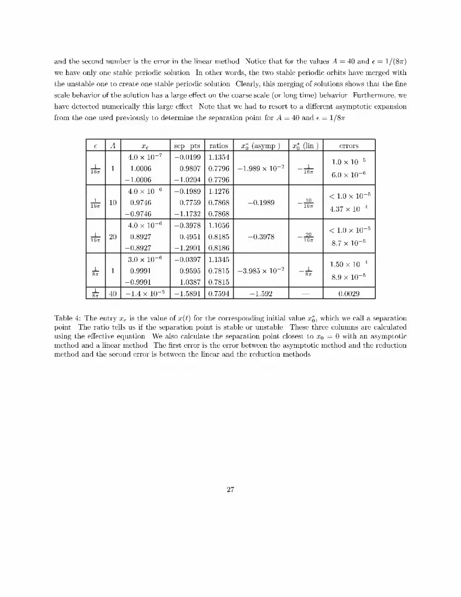
and the second number is the error in the linear method. Notice that for the values A = 40 and � = 1=(8�)we have only one stable periodic solution. In other words, the two stable periodic orbits have merged withthe unstable one to create one stable periodic solution. Clearly, this merging of solutions shows that the �nescale behavior of the solution has a large e�ect on the coarse scale (or long time) behavior. Furthermore, wehave detected numerically this large e�ect. Note that we had to resort to a di�erent asymptotic expansionfrom the one used previously to determine the separation point for A = 40 and � = 1=8�.� A xe sep. pts ratios x�0 (asymp.) x�0 (lin.) errors4:0� 10�7 �0:0199 1:1354116� 1 1:0006 0:9807 0:7796 �1:989� 10�2 � 116� 1:0� 10�5�1:0006 �1:0204 0:7796 6:0� 10�64:0� 10�6 �0:1989 1:1276116� 10 0:9746 0:7759 0:7868 �0:1989 � 1016� < 1:0� 10�5�0:9746 �1:1732 0:7868 4:37� 10�44:0� 10�6 �0:3978 1:1056116� 20 0:8927 0:4951 0:8185 �0:3978 � 2016� < 1:0� 10�5�0:8927 �1:2901 0:8186 8:7� 10�53:0� 10�6 �0:0397 1:134518� 1 0:9991 0:9595 0:7815 �3:985� 10�2 � 18� 1:50� 10�4�0:9991 1:0387 0:7815 8:9� 10�518� 40 �1:4� 10�5 �1:5891 0:7594 �1:592 | 0:0029Table 4: The entry xe is the value of x(t) for the corresponding initial value x�0, which we call a separationpoint. The ratio tells us if the separation point is stable or unstable. These three columns are calculatedusing the e�ective equation. We also calculate the separation point closest to x0 = 0 with an asymptoticmethod and a linear method. The �rst error is the error between the asymptotic method and the reductionmethod and the second error is between the linear and the reduction methods.

27

IV HomogenizationIn the previous sections we discussed only the MRA reduction procedure for nonlinear ODEs. In this sectionwe construct the MRA homogenization scheme for nonlinear ODEs. In the multiresolution approach tohomogenization, the homogenization step is a procedure by which the original system is replaced by someother system with desired properties (perhaps a \simpler" system). By making sure that both systemsproduce the same reduced equations at some coarse scale, we observe that as far as the solution at thethat coarse scale is concerned, the two systems are indistinguishable. We should emphasize that this isa preliminary investigation of the homogenization method for nonlinear ODEs. Homogenizing a nonlinearODE is a di�cult and subtle problem. It is not even clear what constitutes a \simpler" equation.Suppose we reduce our problem to level j, using the series expansion of the recurrence relations, and havea discretization of the form gj(sj)(k) = �j k�1Xk0=0 fj(sj)(k0) + �j2 fj(sj)(k) (4.53)where the functions gj(sj) and fj(sj) are expanded in powers of �j :gj(sj)(k) = 0;j(sj)(k) + 1;j(sj)(k)�2j and fj(sj)(k) = �0;j(sj)(k) + �1;j(sj)(k)�2j :We want to �nd 2j functions ~G(s)(k) and ~F (s)(k) (indexed by k = 0; : : : ; 2�j � 1) with expansions~G(s)(k) = ~G0(s)(k) + �2j ~G1(s)(k) and ~F (s)(k) = ~F0(s)(k) + �2j ~F1(s)(k)such that for each k and all sj 2 Vj we havegj(sj)(k) = 0(sj)(k) + �2j 1(sj)(k) = ~G0(sj)(k) + �2j ~G1(sj)(k)fj(sj)(k) = �0(sj)(k) + �2j �1(sj)(k) = ~F0(sj)(k) + �2j ~F1(sj)(k) (4.54)where ~G1(x)(k) = 124� ~F0(x)(k)~G00(x)(k)�2 ~G000(x)(k) + 112� ~F0(x)(k)~G00(x)(k)� ~F 00(x)(k) and~F1(x)(k) = 124� ~F0(x)(k)~G00(x)(k)�2 ~F 000 (x)(k):In other words, on each interval (k)2�j < t < (k + 1)2�j we want to �nd two functions ~G(x)(k) and~F (s)(k) which depend only on x such that the reduction scheme applied to these functions on each intervalyields the same discretization (4.53) as the original. We know what the �xed point or limiting value of thereduction process for autonomous equations is (see Appendix A) so we may use this exact form to specify~G1(x)(k) and ~F1(x)(k) in terms of ~G0(x)(k) and ~F0(x)(k). We can eliminate ~G1(x)(k) and ~F1(x)(k) from28

the equations (4.54) to get the following coupled system of di�erential equations for each kgj(x)(k) � ~G0(x)(k)�2j = 124� ~F0(x)(k)~G00(x)(k)�2 ~G000 (x)(k) + 112� ~F0(x)(k)~G00(x)(k)� ~F 000 (x)(k)fj(x)(k) � ~F0(x)(k)�2j = 124� ~F0(x)(k)~G00(x)(k)�2 ~F 000 (x)(k):We may pick out the non-oscillatory solution to the system of di�erential equations and obtain~G0 = 0 + �2j� 1 � 124� �0 00�2 000 � 112� �0 00��00�~F0 = �0 + �2j��1 � 124� �0 000 �2�000�:This homogenization procedure will yield a simpli�ed equation which is autonomous over intervals of length2�j and whose solution has the same average over these intervals as the solution to the original, morecomplicated di�erential equation. One can replace the original equation by this homogenized equation andbe assured that the coarse behavior of the homogenized equation is asymptotically equal to the coarsebehavior of the original solution.

29

V ConclusionsWe can extend the MRA reduction and homogenization strategies to small systems of nonlinear di�erentialequations. The main di�culty in extending the reduction procedure to nonlinear equations is that there areno explicit expressions for the �ne scale behavior of the solution in terms of the coarse scale behavior. Weresolve this problem with two approaches; a numerical reduction procedure and a series expansion of therecurrence relations which gives us an analytic reduction procedure.The numerical procedure requires some a priori knowledge of the bounds on the solution since it entailsusing a range of possible values for the solution and its average behavior and working with all of them together.The accuracy of this scheme increases with the square of the initial resolution but it is computationally feasiblefor small systems of equations only. We can use the reduced equation, which we compute numerically, to�nd the periodic orbits of a periodically forced system and to determine the stability of the orbits.One reduction step in the analytic method consists of expanding the recurrence relations in Taylor seriesabout the averages of the solution. We gather the terms in the series which are all of the same order in �j ,the step size, and identify them as one term in the series so that we have a power series in �j . Then we writerecurrence relations for each term in the series so that the nonlinear functions which determine the solutionon the next coarsest scale are themselves power series in the next coarsest step size �j�1. We determine therecurrence relations for an arbitrary term in this power series, show that the recurrence relations converge ifapplied repeatedly, and investigate the convergence of the power series for linear ODEs.The homogenization procedure for nonlinear di�erential equations is a preliminary one. We replace theoriginal equation with an equation which is autonomous on the coarse scale at which we want the solutionsto agree. If we are interested in the behavior of our solution only on a scale 2�j , then our simpler equationwhich we use in place of the original equation does not depend on t over intervals of size 2�j . Unlike thelinear case where a constant coe�cient equation (or an equation with piecewise constant coe�cients) isclearly simpler than a variable coe�cient equation, it is not clear what kind of \simpler" equation shouldreplace a nonlinear equation. We present one candidate type for a simpler equation.

30

VI Appendix AIn this appendix we present several detailed discussions of the series expansion of the recursion relations.The �rst is a derivation of the �xed point of the recurrence relations for autonomous equations. The secondis an algorithm for generating the relations for higher order terms in the power series expansions.More detailed discussions can be found in ([11]). The results include the general forms of the coe�cients (n)0;j (s), (n)1;j (s), �(n)0;j (s), and �(n)1;j (s) in the expansions of g(n)j (s) and f (n)j (s) for non-autonomous di�erentialequations. Conditions for the convergence as n tends to �1 of the recurrence relations for the two lowestorder coe�cients are also discussed. The altered recurrence relations for the case when the left side of thedi�erential equation (2.14), F (t; x(t)), is not Lipschitz as a function of t are given. Finally, the recurrencerelations for the general coe�cients (n)i;j and �(n)i;j are discussed along with the convergence of the seriesexpansions g(n)j (x)(k) = 1Xi=0 (n)i;j (x)(k)�2ij and f (n)j (x)(k) = 1Xi=0 �(n)i;j (x)(k)�2ijunder the reduction process.VI.1 Recursion Relations for Autonomous EquationsWe will now apply the reduction procedure to the autonomous integral equationG(x(t)) = Z t0 F (x(s)) ds (6.55)and examine the series expansions for the recurrence relations when applied to this autonomous integralequation. We will consider only the �rst two terms in the expansions; higher order discretization schemescan be obtained if we keep higher order terms in the expansions.Theorem VI.1 Let us assume that the functions F and G are both twice continuously di�erentiable asfunctions of x and that dGdx 6= 0. Then the coe�cients (n)0;j , (n)1;j , �(n)0;j , and �(n)1;j are given by (n)0;j = G (n)1;j = 13 (22m � 1)22+2m � FG0�F 0 + 13 (22m � 1)23+2m � FG0�2G00�(n)0;j = F �(n)1;j = 13 (22m � 1)23+2m � FG0�2F 00where m = n� j. Furthermore, in the limit as m tends to in�nity, the coe�cients converge to (�1)0;j = G (�1)1;j = 112� FG0�F 0 + 124� FG0�2G00�(�1)0;j = F �(�1)1;j = 124� FG0�2F 00:31

Proof. Because the functions G and F do not depend explicitly on time, the terms gn(xn)(k) and fn(xn)(k)in the initial discretization gn(xn)(k) = �n k�1Xk0=0 fn(xn)(k0) + �n2 fn(xn)(k)are simply the values of G and F evaluated at xn(k). In the non-autonomous case, the terms gn(xn)(k) andfn(xn)(k) are the averages of the function G(t; �) and F (t; �) over the time interval k�n < t < (k + 1)�n andevaluated at xn(k). Because the values gn(sn�1(k))(2k + 1) and gn(sn�1(k))(2k) are equal, the di�erenceoperator D applied to gn and evaluated at sn�1 yields zero,Dgn(sn�1)(k) = 1� �gn(sn�1(k))(2k + 1)� gn(sn�1(k))(2k)� = 0;and the average operator S applied to gn and evaluated at sn�1 yields gn(sn�1)(k),Sgn(sn�1)(k) = 12�gn(sn�1(k))(2k + 1) + gn(sn�1(k))(2k)� = gn(sn�1)(k):We will drop the parameter k in what follows for this reason and simply write G(xn) and F (xn) instead ofgn(xn)(k) and fn(xn)(k) and we will simplify the recursion relations.We begin with an initial discretization of our integral equation at resolution level n = 1 and initialize thecoe�cients as follows (1)0;1(x1) = G(x1) (1)1;1(x1) = 0�(1)0;1(x1) = F (x1) �(1)1;1(x1) = 0:We reduce one level to j = 0 so that the di�erence in resolution (n� j) is one. Using the simpli�ed recursionrelations, we calculate the reduced coe�cients: (1)0;0(x0) = G(x0) (1)1;0(x0) = 116� F (x0)G0(x0)�F 0(x0) + 132� F (x0)G0(x0)�2G00(x0)�(1)0;0(x0) = G(x0) �(1)1;0(x0) = 132� F (x0)G0(x0)�2F 00(x0):We want to �nd the forms of the coe�cients for an arbitrary di�erence in resolution (n � j) = m. Weproceed by induction. Assume that for (n� j) = m we have (n)0;j = G (n)1;j = 13 (22m � 1)22+2m � FG0�F 0 + 13 (22m � 1)23+2m � FG0�2G00 (6.56)�(n)0;j = F �(n)1;j = 13 (22m � 1)23+2m � FG0�2F 00: (6.57)We will apply the simpli�ed recursion relations to these coe�cients and reduce one more level so thatn � (j � 1) = m + 1. It is clear that (n)0;j�1 = G and �(n)0;j�1 = F . The simpli�ed recursion relations tell us32

that (n)1;j�1 = 14S (n)1;j + 116� FG0�F 0 + 132� FG0�2G00= F 0� FG0�� 116 + 14 13 (22m � 1)23+2m �+G00� FG0�2� 132 + 14 13 (22m � 1)23+2m �= 13 (22(m+1) � 1)22+2(m+1) � FG0�F 0 + 13 (22(m+1) � 1)23+2(m+1) � FG0�2G00; and�(n)1;j�1 = 14S�(n)1;j + 132� FG0�2F 00= F 00� FG0�2� 132 + 14 13 (22m � 1)23+2m �= 13 (22(m+1) � 1)23+2(m+1) � FG0�2G00:This proves the formulas (6.56-6.57) for all m = (n�j). Note that these forms depend only on the di�erencein resolution levels n � j. In the limit as m tends to in�nity, we �nd that the coe�cients converge to thefollowing (�1)0;j = G (�1)1;j = 112� FG0�F 0 + 124� FG0�2G00�(�1)0;j = F �(�1)1;j = 124� FG0�2F 00:Additionally, the limiting values of these coe�cients eliminate the error of the initial discretization, give usexpressions independent of resolution level j, and contribute errors only from the truncations of the originalTaylor series. The reduced equation at level j is then given bygj(xj)(k) = �j k�1Xk0=0 fj(xj)(k0) + �j2 fj(xj)(k) where (dropping j) (6.58)g(x)(k) = (1)0 (x(k)) + (1)1 (x(k))�2 and (6.59)f(x)(k) = �(1)0 (x(k)) + �(1)1 (x(k))�2: (6.60)�VI.2 Algorithm to Generate Recurrence RelationsIn subsection II.3, we limited our expansions to O(�2) terms. In this subsection we present an algorithm(implemented in Maple) to compute the recurrence relations for the terms of the power series expansions33

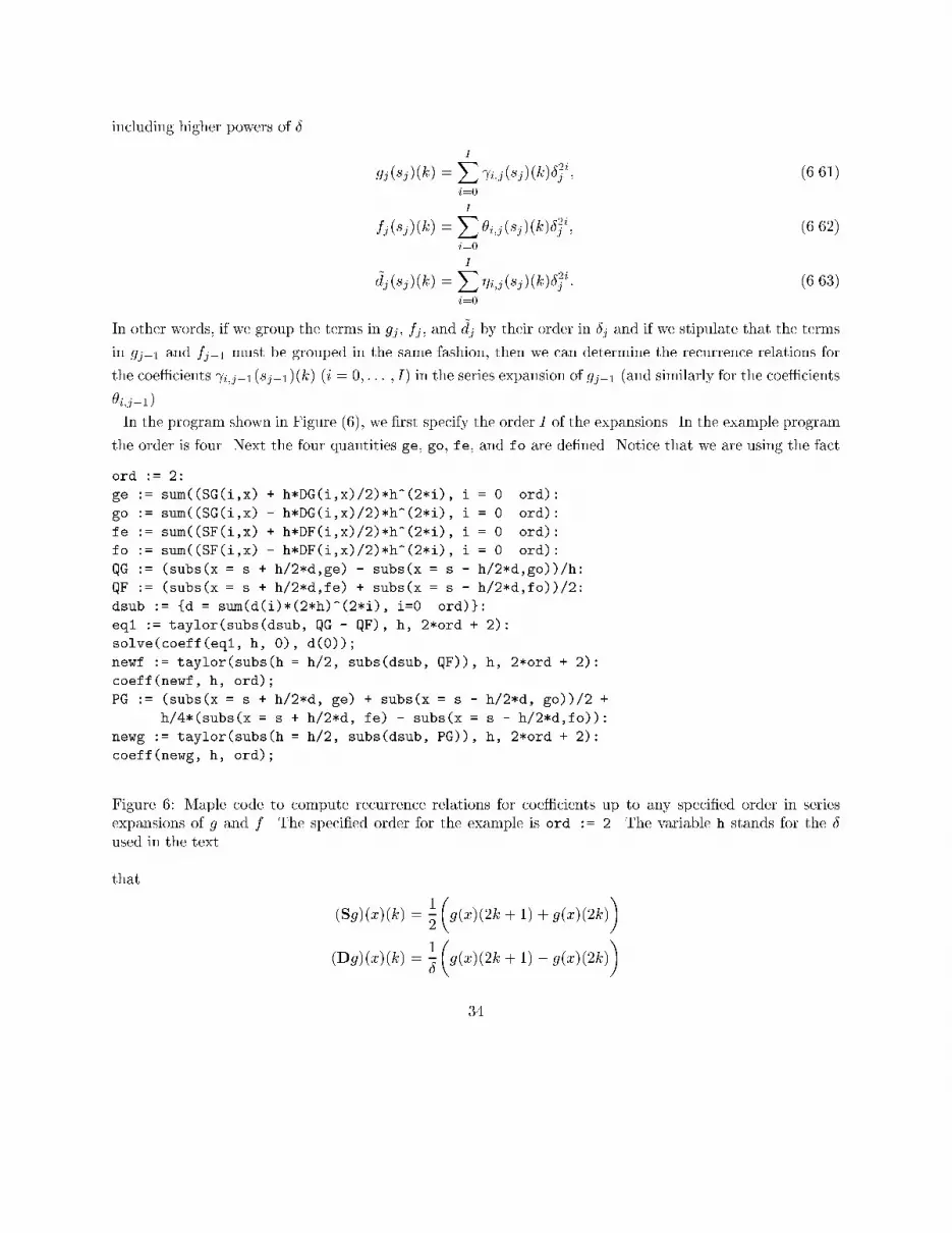
including higher powers of � gj(sj)(k) = IXi=0 i;j(sj)(k)�2ij ; (6.61)fj(sj)(k) = IXi=0 �i;j(sj)(k)�2ij ; (6.62)~dj(sj)(k) = IXi=0 �i;j(sj)(k)�2ij : (6.63)In other words, if we group the terms in gj , fj , and ~dj by their order in �j and if we stipulate that the termsin gj�1 and fj�1 must be grouped in the same fashion, then we can determine the recurrence relations forthe coe�cients i;j�1(sj�1)(k) (i = 0; : : : ; I) in the series expansion of gj�1 (and similarly for the coe�cients�i;j�1).In the program shown in Figure (6), we �rst specify the order I of the expansions. In the example programthe order is four. Next the four quantities ge, go, fe, and fo are de�ned. Notice that we are using the factord := 2:ge := sum((SG(i,x) + h*DG(i,x)/2)*h^(2*i), i = 0..ord):go := sum((SG(i,x) - h*DG(i,x)/2)*h^(2*i), i = 0..ord):fe := sum((SF(i,x) + h*DF(i,x)/2)*h^(2*i), i = 0..ord):fo := sum((SF(i,x) - h*DF(i,x)/2)*h^(2*i), i = 0..ord):QG := (subs(x = s + h/2*d,ge) - subs(x = s - h/2*d,go))/h:QF := (subs(x = s + h/2*d,fe) + subs(x = s - h/2*d,fo))/2:dsub := {d = sum(d(i)*(2*h)^(2*i), i=0..ord)}:eq1 := taylor(subs(dsub, QG - QF), h, 2*ord + 2):solve(coeff(eq1, h, 0), d(0));newf := taylor(subs(h = h/2, subs(dsub, QF)), h, 2*ord + 2):coeff(newf, h, ord);PG := (subs(x = s + h/2*d, ge) + subs(x = s - h/2*d, go))/2 +h/4*(subs(x = s + h/2*d, fe) - subs(x = s - h/2*d,fo)):newg := taylor(subs(h = h/2, subs(dsub, PG)), h, 2*ord + 2):coeff(newg, h, ord);Figure 6: Maple code to compute recurrence relations for coe�cients up to any speci�ed order in seriesexpansions of g and f . The speci�ed order for the example is ord := 2. The variable h stands for the �used in the text.that (Sg)(x)(k) = 12�g(x)(2k + 1) + g(x)(2k)�(Dg)(x)(k) = 1��g(x)(2k + 1)� g(x)(2k)�34

to express ge = g(x)(2k), the even-numbered values of g(x), and go = g(x)(2k + 1), the odd-numberedvalues. The step-size � is accorded the variable h in the program. Next we form the two sides of the equationQG - QF = 0 which determines d̂; at the same time we substitute x(2k+1) = s(k) + h/2d(k) and x(2k)= s(k) - h/2d(k) into ge and fe (respectively, go and fo). Into the expression QG - QF, we substitute theseries expansion for ~d,d = sum(d(i)*(2*h)^(2*i), i=0..ord).We expand the expression QG - QF in a Taylor series and we peel o� the zeroth-order coe�cient in h andsolve for d(0), which gives us the �rst term in our expansion for ~d. This is the recurrence relation for ~�0.To determine higher order terms in the expansion of ~d, we use, for example,simplify(solve(coeff(eq1; h; 2); d(1)));Recall that the recurrence relation for fj is fj = Sfj+1 and notice that Sfj+1 is the same as QF so wesimply substitute the expansion for ~d into QF. Then we let h = h/2 to adjust the resolution size for the nextstep and �nally expand the expression in a Taylor series. (Recall that gj+1 and fj+1 are expanded in powersof �j+1 = �j=2 and gj and fj are expanded in powers of �j .) To determine the recurrence relation for thecoe�cient �i(s)(k), we peel o� the i-th coe�cient (for i � ord):coeff(newf; h; i);:The recurrence relation for gj is given by gj = Sgj+1 + h2=4Dfj+1 which we denote by PG. Again wesubstitute x(2k+1) = s(k) + h/2d(k) and x(2k) = s(k) - h/2d(k) into ge and fe (respectively, go andfo) and we substitute the expansion for ~d into PG. Finally we rescale h and expand PG in a Taylor series. Wedetermine recurrence relations for i(s)(k) in the same fashion as before:coeff(newg; h; i);:We should point out that this is an algorithm for determining the recurrence relation for the coe�cientsin the series (6.61{6.63); however, it does not give a closed form for the recurrence relations.

35

VII Appendix BA multiresolution analysis (MRA) of L2([0; 1]) is a decomposition of the space into a chain of closed subspacesV0 � V1 � � � � � Vn � � �such that [j�0Vj = L2([0; 1]) and\j�0 Vj = fV0g:If we let Pj denote the orthogonal projection operator onto Vj , then limj!1 Pjf = f for all f 2 L2([0; 1]).We have the additional requirements that each subspace Vj (j > 0) is a rescaled version of the base spaceV0: f 2 Vj () f(2j �) 2 V0:Finally, we require that there exists � 2 V0 (called the scaling function) so that � forms an orthonormalbasis of V0. We can conclude that the set f�j;kj k = 0; : : : ; 2j�1 g is an orthonormal basis for each subspaceVj . Here �j;k denotes a translation and dilation of �:�j;k = 2j=2�(2jx� k):As a consequence of the above properties, there is an orthonormal wavelet basisf j;kj j � 0; k = 0; : : : ; 2j � 1 gof L2([0; 1]), j;k(x) = 2j=2 (2jx� k), such that for all f in L2([0; 1])Pj+1f = Pjf + 2j�1Xk=0 hf; j;ki j;k:If we de�ne Wj to be the orthogonal complement of Vj in Vj+1, thenVj+1 = Vj �Wj :We have, for each �xed j, an orthonormal basis f j;kjk = 0; : : : ; 2j�1 g for Wj . Finally, we may decomposeL2([0; 1]) into a direct sum L2([0; 1]) = V0Mj�0Wj :The operator Qj is the orthogonal projection operator onto the space Wj .The Haar wavelet and its associated scaling function � are de�ned as follows:�(x) = � 1; x 2 [0; 1)0; elsewhere and (x) =8<: 1; x 2 [0; 1=2)�1; x 2 [1=2; 1)0; elsewhere:36

References[1] A. Askar, B. Space, and H. Rabitz. The subspace method for long time scale molecular dynamics.preprint, 1995.[2] C. M. Bender and S. A. Orszag. Advanced methods for scientists and engineers. McGraw-Hill, Inc.,New York, 1978.[3] A. Bensoussan, P. L. Lions, and G. Papanicolaou. Asymptotic analysis for periodic structures. North-Holland Publ. Co., The Netherlands, 1978.[4] G. Beylkin, R. Coifman, and V. Rohklin. Fast wavelet transforms and numerical algorithms I. Comm.Pure Appl. Math., 44, 1991.[5] G. Beylkin and N. Coult. A multiresolution strategy for reduction of elliptic PDE's and eigenvalueproblems. preprint, 1996.[6] Folkmar Bornemann and Christof Sch�utte. Homogenization of hamiltonian systems with a strongconstraining potential. to appear in Physica D, 1997.[7] M. E. Brewster and G. Beylkin. A multiresolution strategy for numerical homogenization. Appl. andComp. Harmonic Analysis, (2) 4, 1995.[8] R. Coifman, P. L. Lions, Y. Meyer, and S. Semmes. Compensated compactness and hardy spaces. J.Math. Pures Appl., 72, 1993.[9] M. Dorobantu. Wavelet-based algorithms for fast PDE solvers. PhD thesis, Royal Institute of Technol-ogy, Stockholm University, 1995.[10] A. C. Gilbert. A comparison of multiresolution and classical one-dimensional homogenization schemes.Appl. and Comp. Harmonic Analysis, 1996.[11] A. C. Gilbert. Multiresolution homogenization schemes for di�erential equations and applications. PhDthesis, Princeton University, 1997.[12] V. V. Jikov, S. M. Kozlov, and O. A. Oleinik. Homogenization of di�erential operators and integralfunctionals. Springer-Verlag, New York, 1994.[13] J. Kervorkian and J. D. Cole. Perturbation methods in applied mathematics. Springer-Verlag, NewYork, 1985.[14] P. A. Lagerstrom. Matched asymptotic expansions, ideas and techniques. Springer-Verlag, New York,1988. 37

[15] F. Murat. Compacit�e par compensation. Ann. Scuola Norm. Sup. Pisa Cl. Sci., (4) 5, 1978.[16] Christof Sch�utte and Folkmar Bornemann. Homogenization approach to smoothed molecular dynamics.preprint, 1997.[17] B. Space, H. Rabitz, and A. Askar. Long time scale molecular dynamics subspace integration methodapplied to anharmonic crystals and glasses. J. Chem. Phys., 99 (11), 1993.[18] L. Tartar. Compensated compactness and applications to partial di�erential equations. Heriot-WattSympos., IV, 1979.

38