A multi-way analysis of starch cassava properties

A multi-way analysis of starch cassava properties

Marlon M. Reis a, Marcia M.C. Ferreira a,*, Silene B.S. Sarmento b

aChemistry Institute-UNICAMP, Cidade Universitaria Zeferino Vaz, s/n, PO Box 6154, 13083-970 Campinas, Sao Paulo, BrazilbDepartment of Agroindustry, Food and Nutrition, Escola Superior de Agricultura ‘‘Luiz de Queiroz’’, Universidade de Sao Paulo, Brazil

Received 31 August 2001; received in revised form 18 June 2002; accepted 26 June 2002

Abstract

The original methods proposed by Ledyard R. Tucker during the 1960s present the rotational freedom problem, making the

interpretation of their results rather difficult to be carried out. Aiming to make the multi-way data analysis more acceptable, this

work suggests a methodology for extracting meaningful information from the data set. This methodology is based on the

decomposition of data set in three-way blocks by using Tucker models. With the aim of keeping in one block similar

information about the data properties, a decomposition based on a constrained Tucker model was used, where the core array has

some of its elements fixed to zero. This methodology is successfully applied to a data set formed by physical and

physicochemical properties of starches of four cassava cultivars, harvested at different ages during the period usually taken for

harvest of industrial uses.

D 2002 Elsevier Science B.V. All rights reserved.

Keywords: Constrained Tucker model; Cassava starch properties; Multi-way analysis

1. Introduction

The Tucker models introduced by Tucker [1] dur-

ing the 1960s for the interpretation of psychological

data have been applied to three-way environmental [2]

and chemical data for exploratory analysis [3], iden-

tification of compounds and second order calibration

[4], among others. The original methods proposed by

Tucker present the rotational freedom problem, mak-

ing the interpretation of its results rather difficult to be

carried out [5]. A procedure presented to avoid such

problem is the rotation of the component matrices of

the fitted model. An alternative approach is based on

constraining certain parameters in the Tucker model to

zero. In such instances, fitting the constrained Tucker

model to data set is not meant for assessing which

model should be used to describe the data, but for

determining which parameter values govern certain

aspects of the data [5].

Starch composition and its properties vary mainly

with the plant source from which it is derived [6,7]. It

is the main constituent of cassava roots. The industrial

uses of starch are primarily determined by its phys-

ical–chemical properties. This work deals with a data

set formed by the properties of four cassava cultivars,

harvested at different ages during the period usually

taken for harvest of industrial uses [6].

0169-7439/02/$ - see front matter D 2002 Elsevier Science B.V. All rights reserved.

PII: S0169 -7439 (02 )00053 -9

* Corresponding author. Tel.: +55-19-3788-3102; fax: +55-19-

3788-3023.

E-mail address: [email protected] (M.M.C. Ferreira).

www.elsevier.com/locate/chemometrics

Chemometrics and Intelligent Laboratory Systems 64 (2002) 123–135

The complexity of the data set, age and genetic

factors makes the data analysis rather complex. The

multivariate data analysis on a subset of this data by

principal component analysis [8] confirms the impor-

tance of using chemometric methods in such kind of

study. This data complexity demands the application

of more sophisticated methods such as three-way

methods.

The methodological aspect of this work lies on the

evaluation of the possibility of extracting meaningful

information from the data set. It is based on the

decomposition of the data set in three-way blocks

by using Tucker models in such a way to keep in one

block the similar information of starch properties

among the cultivars. Three decompositions were

tested: the first being a Tucker model without con-

straints, the second is originated by rotation of the first

model and the last one is a constrained Tucker model

inspired on the models presented by Kiers et al. [9],

where the core array had part of its elements fixed to

zero.

The goal of this work is to provide information

about carrying out an exploratory data analysis by

three-way methods suggesting some tools such as

inertia functions for the evaluation of the fitted mod-

els. These abilities were verified by the meaningful

information extracted from the data set used.

2. Notation

See Appendix A.

3. Data description

The data set consists of the results from exper-

imental measurements of physicochemical and func-

tional properties of starch extracted from four

cassava cultivars (i.e. Manihot esculenta Crantz:

SRT 59-Branca de Santa Catarina, SRT 1287-Fibra,

SRT 1105 Mico and IAC 12-829), growing in

Campinas, Sao Paulo State (Brazil) and harvested

at eight different ages, 10, 12, 14, 16, 18, 20, 22 and

24 months after being planted (i.e. the first harvest

July and the last one in September of the following

year). As the harvest period is long, the roots are

subjected to well-defined climatic conditions in this

region: a rainy season with high temperatures and

rainfall, and a drought season with low temperatures

and rainfall. The variables studied were: amylose

content (AC); granule absolute density (GAD); swel-

ling power (SP) and solubilities (%S) at 60, 75 and

90 jC; water-binding capacity (WBC); enzymatic

susceptibility (Glu) expressed in amount of reducing

sugars produced after 3, 6 and 24 h; granular

specific surface area (GSSA) and pasting properties:

peak of viscosity (PV) and retrogradation (R)1.

These experimental results can be arranged in a

three-way data array with modes (age� proper-

properties� cultivars).

4. Preprocessing

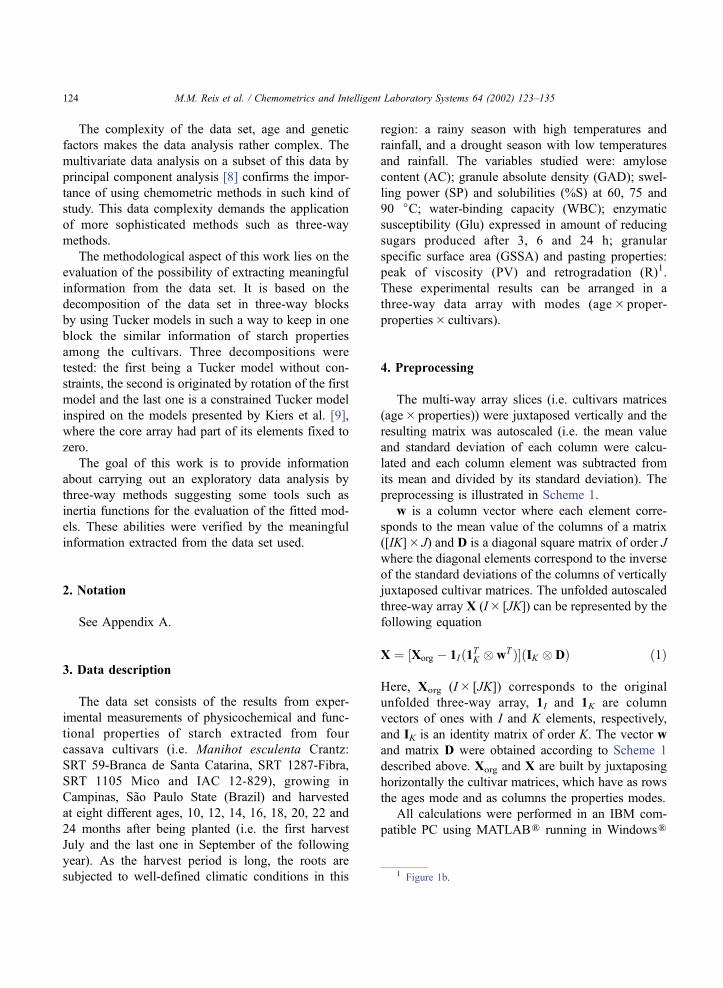
The multi-way array slices (i.e. cultivars matrices

(age� properties)) were juxtaposed vertically and the

resulting matrix was autoscaled (i.e. the mean value

and standard deviation of each column were calcu-

lated and each column element was subtracted from

its mean and divided by its standard deviation). The

preprocessing is illustrated in Scheme 1.

w is a column vector where each element corre-

sponds to the mean value of the columns of a matrix

([IK]� J) and D is a diagonal square matrix of order J

where the diagonal elements correspond to the inverse

of the standard deviations of the columns of vertically

juxtaposed cultivar matrices. The unfolded autoscaled

three-way array X (I� [JK]) can be represented by the

following equation

X ¼ ½Xorg � 1I ð1TK � wT Þ�ðIK � DÞ ð1Þ

Here, Xorg (I� [JK]) corresponds to the original

unfolded three-way array, 1I and 1K are column

vectors of ones with I and K elements, respectively,

and IK is an identity matrix of order K. The vector w

and matrix D were obtained according to Scheme 1

described above. Xorg and X are built by juxtaposing

horizontally the cultivar matrices, which have as rows

the ages mode and as columns the properties modes.

All calculations were performed in an IBM com-

patible PC using MATLABR running in WindowsR

1 Figure 1b.

M.M. Reis et al. / Chemometrics and Intelligent Laboratory Systems 64 (2002) 123–135124

system. The Multi-Way toolbox (version 1.08, Oct.

1998) was downloaded from Internet [10].

5. Theory

5.1. Tucker model

Tucker model is the most general model for three-

way data. For a three-way array, it is given by Eq. (2).

xijk ¼XPp¼1

XQq¼1

XRr¼1

aipbjqckrgpqr

!þ eijk ð2Þ

where aip, bjq and ckr denote elements of the compo-

nent matrices A (for A mode), B (for B mode) and C

(for C mode) of order I�P, J�Q and K�R, respec-

tively. Furthermore, gpqr denotes the element ( p,q,r)

of the P�Q�R core array G. Finally, eijk denotes the

error term for element xijk when approximated by a

Tucker model and is an element of the I� J�K array

E.

The matrix formulation for the Tucker model is

given by Eq. (3).

X ¼ AGðCT � BT Þ þ E ð3Þ

where A, B and C denote the component matrices of

order I�P, J�Q and K�R, respectively, G denotes

the unfolded core array of order (P� [QR]) and

finally, E denotes the error term by approximating X

by the Tucker model.

In this work, it is considered the decomposition of

the Tucker model in R blocks as demonstrated by Eq.

(4), where each term ‘‘AGr(crT�BT)’’ corresponds to

one block.

X ¼ AG1ðcT1 � BT Þ þ AG2ðcT2 � BT Þ þ : : :

þ AGRðcTR � BT Þ þ E ð4Þ

5.2. Inertia functions

Tucker models are fitted by the alternating least

squares (ALS) algorithm [11], where the loss function,

Eq. (5), is minimized.

lossðA;B;C;GÞ ¼ NX� AGðCT � BT ÞN2 ð5Þ

The goodness of the ALS algorithm fitting is

usually checked by the amount of explained inertia

[3]. In this work, the Tucker models were evaluated

by means of two kinds of ‘‘inertia function’’, which

informs how good is the fitting. The first, ‘‘total

inertia function’’, given by Eq. (6), is based on the

Scheme 1.

M.M. Reis et al. / Chemometrics and Intelligent Laboratory Systems 64 (2002) 123–135 125

loss function which is minimized by the ALS used to

fit the Tucker models.

f ¼ 1� NX� AGðCT � BT ÞN2

NXN2

!� 100% ð6Þ

The other function, ‘‘partial inertia function’’, Eq.

(7), is used to verify how the core slices describe each

slice of the data array.

5.3. Partial inertia function

f ðGk ; cqk ;XqÞ

¼ 1�NvecXq � ½ðA� BÞvecGkcqk �N2

vecXTq vecXq

!� 100% ð7Þ

where vecXq is the data array slice reshaped as a

column vector by the operator vec, vecGk is the core

slice reshaped as a column vector and cqk is a C-mode

component matrix element.

5.4. Rotated Tucker model

The rotated Tucker model is generated by rotating

the core array using an Orthomax [12] rotation for the

three modes as follows:

X ¼ ASSTGðU� TÞðUT � TT ÞðCT � BT Þ ð8Þ

since

SST ¼ STS ¼ I; UTU ¼ UUT ¼ I;

TTT ¼ TTT ¼ I ð9Þ

then

X ¼ eAeGðeCT � eBT Þ ð10Þ

takingeA ¼ AS; eG ¼ STGðU� TÞ; eC ¼ CU; eB¼ BT ð11Þ

where S, T and U are the rotation matrices for the A,

B and C modes, respectively, and Af

, Bf

and Cf

corresponds to the rotated component matrices.

5.5. Constrained Tucker model

The constrained Tucker model fits a Tucker model

subject to certain constraints on the core. In this case,

some elements of the constrained core are fixed to

zero. It is also fitted by the ALS algorithm, having as

difference the update of the core elements [5,9].

5.6. Methodology

The methodology described in this work for the

multi-way data analysis is based in a multi-way

decomposition in which the information about the

starch properties, common among the cultivars, is

captured in a block (AGr(crT�BT) in Eq. (4)). For

that, the first assumption used in the analysis is that at

least one vector of the component matrix, which

represents the cultivars mode, must be nonnegative

(or to have all the elements with same sign). This

assumption suggests that this(ese) vector(s) represents

the same kind of information in all cultivars but with

different weights. In this case, if any element of vector

cr, for block AGr(crT�BT), has a different sign from

the others, it means that the information described by

AGrBT for this element will be the opposite of the

other elements of cr (i.e. each element represents a

slice of the C mode, in this work, a cultivar matrix).

To make this assumption more clear, consider as an

example the total luminescence experiment based on

the excitation of a sample in a range of wavelengths

resulting in a spectrum of emission intensities for each

exciting wavelength [13]. As a result, for each sample

there is an emission intensity surface (i.e. excita-

tion� emission). If there is more than one sample,

the data set corresponds to a three-way array (i.e.

excitation� emission� sample). In this case, if an

absorbing specie is present in all samples but in

different concentrations, the emission intensity surface

for this species corresponds to the ‘‘same kind of

information’’ (the emission intensity surface is unique

for each species at unity concentration) present in all

samples but in different ‘‘weights’’ (concentrations).

In the present work, only one vector can be non-

negative (or negative) due to the orthogonality con-

straint applied in the component matrices (i.e. A, B,

and C) for the three modes. Therefore, the core slice

associated with this component vector should repre-

sent the similar relationship between the plants age


and their properties for all cultivars. In this way, the

aim of this multi-way data analysis is to extract the

information about the starch properties during the

studied period, which is similar for all cultivars.

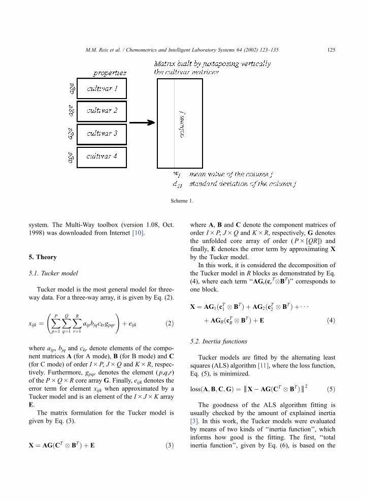
The constrained Tucker model has as fundamental

problem in designing the core array, in other words,

how to choose the core elements that should be fixed

to zero. In some applications, the core design is based

on the data characteristics [5]. In the exploratory

analysis context, the core design should have a struc-

ture that makes the data analysis easily carried out.

Additionally, the information in one block should be

independent from the other blocks. Thus, the elements

to be fixed to zero in the constrained core are chosen

in this work, at first, considering the orthogonality of

the vectors in VEC(GC) (the orthogonality is imposed

by the restriction that the nonfixed elements in one

slice must be fixed as zero in the other slices), second,

by considering the results of the rotated Tucker model

and, finally, the values of the partial inertia function

which must be nonnegative. In this way, the first

constrained slice of the core array to be built is that

one associated with the nonnegative vector of the C-

mode component matrix found in rotated Tucker

model. This is done by choosing the elements, to be

fixed to zero, as those having small values on the

respective core slice fitted by rotated Tucker model.

The second slice is built considering the values

magnitude for the respective core elements of rotated

Tucker model and the restriction that the nonfixed

elements in one slice must be fixed to zero in the other

slices. The last parameter to be considered is the

function f(GG� qk), the partial inertia function, which

must be nonnegative for all core slices and data slices.

In this way, a constrained Tucker model is fitted and

f(GG� qk) is verified for negative values. If there is one

or more negative values, a new constrained model is

built and fitted again. A simple example on building

the core slices is given in Scheme 2.

6. Results

The first analysis was carried out using the va-

riables amylose content (AC); granule absolute density

Table 1

Singular values for cultivar mode matrices (age� properties),

horizontally and vertically juxtaposed

Singular values

BSCa Micoa Fibraa IACa X1b X2c

1 7.9349 4.6923 5.0551 5.9045 10.8104 10.0823

2 4.2190 3.9153 4.1699 3.9585 8.8409 8.3358

3 3.1204 3.4352 3.8742 3.5939 6.5597 6.5593

4 2.3468 2.8444 3.4254 2.8041 6.3111 6.0054

5 2.0159 2.2793 2.9542 2.4515 4.6355 5.1407

6 1.4671 1.8580 2.2703 1.6155 4.3996 4.8358

7 1.0417 1.5234 1.6500 1.2270 3.7283 4.1320

8 0.4981 0.4314 0.7402 0.8817 2.8932 3.0891

a Cultivars matrices.b Vertically juxtaposed cultivar matrices.c Horizontally juxtaposed cultivar matrices.

Scheme 2.


(GAD); swelling power (SP) and solubilities (%S) at 60

and 90 jC; water-binding capacity (WBC); enzymatic

susceptibility (Glu) expressed in amount of reducing

sugars produced after 3, 6 and 24 h; granular specific

surface area (GSSA). These data form a three-way data

array with modes (age� properties� cultivars) having

the dimension (8� 11� 4).

The singular values calculated for scaled data slices

and of juxtaposed matrices presented in Table 1

suggest that the rank of the matrices is 8 for the data

slices. Thus, Tucker models were fitted with dimen-

sion for the A, B and C modes as (8� 8� 4),

respectively. The Tucker model fitted 95.80% as

measured by the inertia function given in Eq. (6)

and constrained Tucker model fitted 85.81%.

Table 2 presents the C-mode nonnegative vectors

for the three models. In this table, it is possible to notice

that vectors for a rotated Tucker model and a con-

strained Tucker model present more similar values, a

good aspect since the block corresponding to this

vector, should describe the starch properties, which is

supposed to be similar among plant varieties. Although

the nonnegative vectors for the fitted models have

presented meaningful variation among their values,

the partial inertia function presented negative values

for the rotated Tucker model as shown in Table 3. In

spite of these negative values being small, they suggest

which of the corresponding core slices kept more

information than it should have. In other words, the

distribution of values in the nonnegative vectors has no

physical meaning for the rotated Tucker model, even

being correctly calculated as shown in Appendix B.

Table 4 shows the partial inertia function values

associated with the nonnegative vectors of the three

models; it can be noticed that the vector elements for

the constrained Tucker model are more similarly

distributed.

The partial inertia function values were important in

order to determine the best-fixed to zero positions in

the constrained Tucker model core array since the best

combination was that one which provided nonnegative

values for partial inertia function. The partial inertia

function values used as parameter yield information on

how the constrained Tucker model describes the data.

Negative values for partial inertia function indicates

that the nonmodeled part of the data has large influ-

ence as shown in Appendix B.

Table 5 shows the core slice for the constrained

Tucker model corresponding to the nonnegative vec-

tor in the C mode. The element in column 6 and row 7

is the third most important of all core elements. This

element corresponds to vector 7 of A-mode compo-

nent matrix, a7, and vector 6 of B-mode component

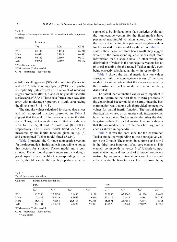
matrix, b6. a7 gives information about the seasonal

effects on starch characteristics. Fig. 1a shows the a7

Table 2

Loadings of nonnegative vector of the cultivar mode component

matrices

Loadings

TM RTM CTM

BSC 0.2141 0.4738 0.4718

Mico 0.4636 0.4886 0.4981

Fibra 0.6163 0.4607 0.5107

IAC 0.5995 0.5697 0.5182

TM—Tucker model.

RTM—rotated Tucker model.

CTM—constrained Tucker model.

Table 3

Partial inertia function values

Cultivars Partial inertia function (%)

RTM CTM

G1a G2

a G3a G4

a G1a G2

a G3a G4

a

BSC 60.3390 22.7970 0.8486 1.8170 26.2985 62.3342 0.1074 0.4401

Mico � 0.4535 52.9419 � 1.3969 42.6410 50.6217 0.0115 3.4313 26.7182

Fibra 35.8150 47.6668 26.5168 � 0.3346 45.6891 25.7686 7.2344 7.9505

IAC 20.8181 57.8973 7.4225 9.3023 49.4570 16.2763 17.0759 0.7268


CTM—constrained Tucker model.a Core slices.


vector, where there are two distinct groups: the first is

formed by samples corresponding to the ages of 10,

22 and 24 months (cold and dry season) and the

second to the ages of 12, 14, 16, 18 and 20 months

(hot and rainy season).

The first group corresponds to the drought period

when the plants do not produce or produce only minor

amounts of starch or consume this component to

provide plant physiology needs, since there was the

loss of leaves, followed by the renewal of the plant

top. The second group represents the rainy season,

stage when there is intense root formation and starch

accumulation. It is interesting to notice the correlation

between values of the age of the plants and the vector

values in the second group. The information repre-

sented by the vectors a7 and b6 is uniquely determined

since only one core slice of constrained Tucker model

has the column 6 and row 7 with only one element not

fixed to zero. The results presented by the a7 vector

confirm the ability of the constrained Tucker model to

keep in one block the common information about the

starch structure.

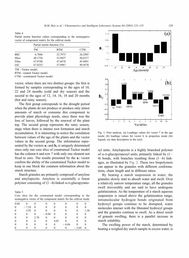
Starch granules are primarily composed of amylose

and amylopectin. Amylose is essentially a linear

polymer consisting of (1–4)-linked a-D-glucopyrano-

syl units. Amylopectin is a highly branched polymer

of a-D-glucopyranosyl units, primarily linked by (1–

4) bonds, with branches resulting from (1–6) link-

ages, as illustrated by Fig. 2. These two biopolymers

can appear in the granules with different conforma-

tions, chain length and in different ratios.

By heating a starch suspension in water, the

granules slowly start to absorb water and swell. Over

a relatively narrow temperature range, all the granules

swell irreversibly and are said to have undergone

gelatinization. As the temperature of a starch aqueous

suspension is raised above the gelatinization range,

intramolecular hydrogen bonds originated from

hydroxyl groups continue to be disrupted, water

molecules interact with the liberated hydroxyl groups

and the granules continue to swell. As a direct result

of granule swelling, there is a parallel increase in

starch solubility.

The swelling power of the starch, determined by

heating a weighed dry starch sample in excess water, is

Table 4

Partial inertia function values corresponding to the nonnegative

vector of component matrix for the cultivar mode

Partial inertia function (%)

TM RTM CTM

BSC 6.7886 22.7973 26.2985

Mico 48.1736 52.9427 50.6217

Fibra 67.0748 47.6670 45.6891

IAC 67.0252 57.8967 49.4570

TM—Tucker model.


CTM—constrained Tucker model.

Table 5

Core slice for the constrained model corresponding to the

nonnegative vector of the component matrix for the cultivar mode

0.04 0 0 0 0 0 0 0

0 � 7.10 0 0 0 0 0 0

0 3.93 0 0 0 0 0 1.38

0 0 0 � 0.94 0 0 0 0

0 0 2.76 0 0 0 0 0

0 0 0 0 4.03 0 0 0

0 0 0 0 0 � 6.04 0 0

0 0 0 0 0 0 � 3.64 0

Fig. 1. First analysis. (a) Loadings values for vector 7 in the age

mode; (b) loadings values for vector 6 in properties mode (for

legend, see data description in the text).


defined as the swollen sediment weight per gram of dry

starch. The solubilities can also be determined on the

same solution [6,7]. According to Leach [14], the

strength and character of micellar network within the

granule are the major factors controlling swelling

behavior of starch. At molecular level, many factors

may influence the degree and kind of association

between the polymers (i.e. amylose and amylopectin).

These factors include the ratio of amylose to amylo-

pectin, the characteristics of each fraction in terms

of molecular weight/distribution, degree/length of

branching and conformation of these polymers. The

presence of the naturally occurring noncarbohydrates

such as lipids is also an important factor. The formation

of amylose–lipid complexes can restrict swelling and

solubilization. The difference in the solubility behavior

of the root may be attributed to differences in the

conformation of the amylose components in native

starch granules. In root starches, lipids are almost

absent and the amylose occurs in amorphous state

and is converted by heat treatment into a less soluble

helical form [6,7]. The loadings in vector b6 for

swelling power and solubilities (see Fig. 1b: SP-60,

%S60, %S90, swelling power at 60 jC and percentage

of solubilities at 60 and 90 jC) presented a positive

correlation with the first group (i.e. samples at age of

10, 22 and 24 months) and a negative correlation with

the second group (i.e. samples 12, 14, 16, 18 and 20

months old). The signs of these loadings are opposite to

amylose content loading. The values of loadings for

solubilities suggest that the difference between those

two sample groups is due to amylose conformation and

not due to the amount of this macromolecule.

Water molecules, which interact with the macro-

molecules, are termed ‘bound water’, and reflect the

ability of a molecular surface to form hydrogen bonds

Fig. 2. Chemical structure of a-amylose and amylopectin macromolecules.


with water. The molecular surface available for such

‘binding’ of water molecules are reduced in the regions

with extensive intramolecular hydrogen bonds. The

amount of ‘bound water’ associated with starch gran-

ules influences the swelling characteristics of the

granules. High ‘water-binding’ is attributed to the loss

of association ability of the starch polymers in native

granule. The water-binding sites are considered to be

the hydroxyl groups and their interglucose oxygen

atoms. During the gelatinization process, the water-

binding sites are increased as the heat starts to disrupt

the intragranular bonds [6,7]. The loadings in vector b6for water-binding capacity (see Fig. 1b, WBC) pre-

sented positive correlation with amylose and the sec-

ond group (i.e. samples at the age of 12, 14, 16, 18 and

20 months). It presented also negative correlation with

the first group (i.e. samples at the age of 10, 22 and 24

months), swelling power and solubilities. These differ-

ences between those two sample groups are due to the

amount of amylose and to the existence of a different

number of water-binding sites, which suggests differ-

ent proportions of amorphous/crystalline areas.

The loadings for granular specific surface area

(GSSA) and granule absolute density (GAD) are

opposite in signs. The granule absolute density is

positively correlated to the first group and the granular

specific surface area is positively correlated to the

second group. The specific granule surface area is

inversely proportional to granule size. This indicates

that the first group contains granules bigger in size

and more compact than the second group.

The susceptibility of starch granules to digestion

by glucoamylase was evaluated by measuring the

amount of glucose units (i.e. reducing sugars) pro-

duced after a period of enzymatic attack. The glucoa-

mylase cleaves the a(1–4) and a(1–6)-linkages of

starch chain producing glucose units. The amorphous

part in starch granule is more susceptible to enzymatic

attack, making possible the use of enzymatic degra-

dation to study the ratio between the amorphous and

the crystalline parts in starch granule. The loadings

related to the amount of reducing sugars after 3 and 6

h are positively correlated with amylose content,

water-binding capacity and granular specific surface

area (granules smaller in size) and with the second

group. Amount of reducing sugar produced after 24 h

is positively correlated to swelling power (60) and

solubilities (60,90) and to the first group.

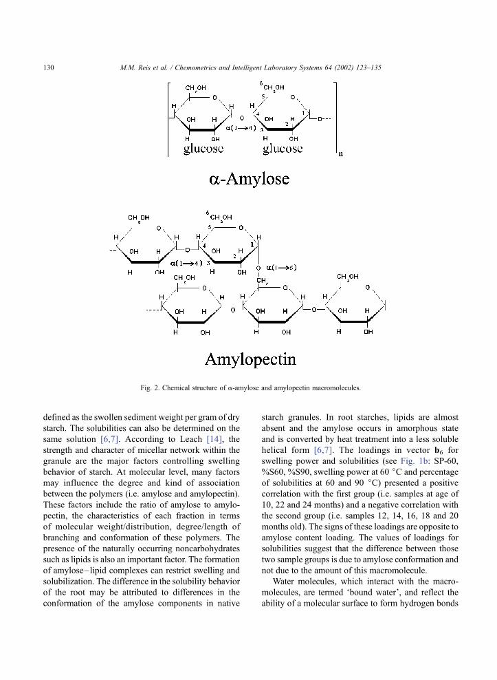
Two new analyses were done. Firstly, variables

about the pasting properties were included. For the

second analysis, variables about the pasting properties

and swelling power (%SP) and solubilities at 75 jCwere included, while the variable of the amount of

reducing sugar produced after 24 h was excluded.

This was done to verify if the constrained Tucker

model would extract the same kind of information in

both instances: by including or excluding new varia-

bles. The results are shown in Figs. 3 and 4.

The pasting properties showed higher viscosity

peaks for starches of the first group and these peaks

were negatively correlated to amylose content, water-

binding capacity, enzymatic susceptibility and granule

specific surface area (or lower size granules). Retro-

gradation was negatively correlated with viscosity

peaks and positively correlated with amylose amounts,

the last one being recognized as the main factor

influencing this property.

The loadings in vector b6 show positive correla-

tion among water-binding capacity (more water-bind-

Fig. 3. Second analysis. (a) Loadings values for vector 7 in the age




ing sites), production of reducing sugars in short

periods (more susceptible regions for enzymatic

attack), specific granule surface area (smaller granule

size) and amylose content. These properties and

composition are negatively correlated to granule

density, swelling power and solubilities and produc-

tion of reducing sugars in long period. These corre-

lations indicate that the granules of samples in the

first group (for rainy season, i.e. 10, 22 and 24

months old, see Figs. 1, 2 and 3a) are more compact

with less amorphous regions. Whereas the second

group of samples (drought conditions, i.e. samples

12, 14, 16, 18 and 20 months old, see Figs. 1, 3 and

4a) present less compact granules having probably

more amorphous regions which are associated with

the amylose content.

It should be noticed that the a7 vector presents an

aging gradient. In short, it is positive for the age of 10

months, then its values decrease gradually until the

age of 18, and finally its values increase gradually

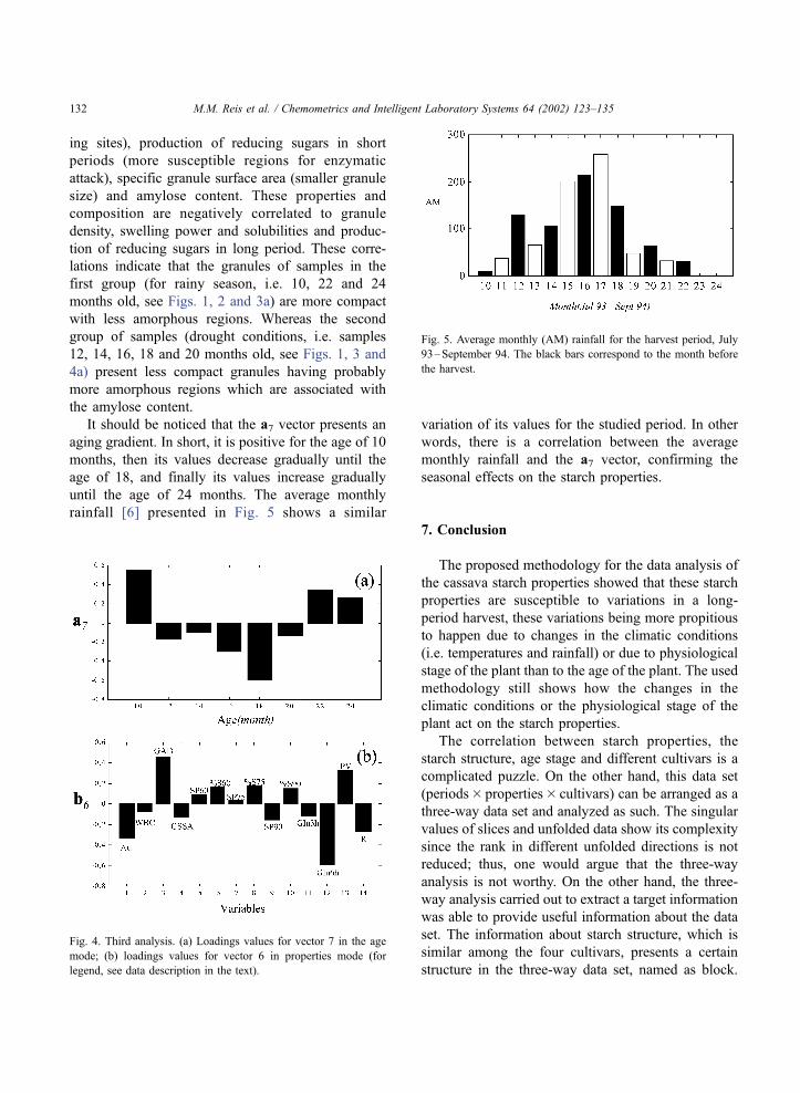
until the age of 24 months. The average monthly

rainfall [6] presented in Fig. 5 shows a similar

variation of its values for the studied period. In other

words, there is a correlation between the average

monthly rainfall and the a7 vector, confirming the

seasonal effects on the starch properties.

7. Conclusion

The proposed methodology for the data analysis of

the cassava starch properties showed that these starch

properties are susceptible to variations in a long-

period harvest, these variations being more propitious

to happen due to changes in the climatic conditions

(i.e. temperatures and rainfall) or due to physiological

stage of the plant than to the age of the plant. The used

methodology still shows how the changes in the

climatic conditions or the physiological stage of the

plant act on the starch properties.

The correlation between starch properties, the

starch structure, age stage and different cultivars is a

complicated puzzle. On the other hand, this data set

(periods� properties� cultivars) can be arranged as a

three-way data set and analyzed as such. The singular

values of slices and unfolded data show its complexity

since the rank in different unfolded directions is not

reduced; thus, one would argue that the three-way

analysis is not worthy. On the other hand, the three-

way analysis carried out to extract a target information

was able to provide useful information about the data

set. The information about starch structure, which is

similar among the four cultivars, presents a certain

structure in the three-way data set, named as block.

Fig. 4. Third analysis. (a) Loadings values for vector 7 in the age



Fig. 5. Average monthly (AM) rainfall for the harvest period, July

93–September 94. The black bars correspond to the month before

the harvest.


This three-way structure, block, was best approxi-

mated by constrained Tucker model. The formulation

of the constrained Tucker model was done by consid-

ering the independence among blocks, which was

formulated theoretically. The inertia function, which

gave information about how the data slices are

described by the core slice, was fundamental for the

final adjustment of the constrained Tucker model.

This methodology is interesting since the vectors in

the A mode and B mode which show the correlation

between properties and age are directly related in one

block, making its analysis quite easy.

The information presented by the constrained

Tucker model is helpful for choosing the best period

to harvest cassava plants since these properties are

important for food and industrial use of its starch.

Acknowledgements

The authors acknowledge the financial support

from FAPESP (grant number 97/13046-4) for carrying

out this work and also Prof. Dr H.A.L. Kiers for

sharing the Orthomax codes.

Appendix A

Notation

Xq ¼ qx1 qx2: : :qxMð Þ The q slice matrix of a three-way array; qx1. . .M are column vectors

X ¼ X1A X2A : : :A XOð Þ;G ¼ G1A G2A : : :A GRð Þ

Unfolded three-way arrays (N� [MO]) and ( P� [QR])

A ¼ a1 a2 : : : aPð Þ;B ¼ b1 b2 : : : bQð Þ;C ¼ c1 c2 : : : cRð Þ

Loading matrices (component matrices)

a1 ¼ a11 a21 : : : aN1ð ÞT ;b1 ¼ b11 b21 : : : bM1ð ÞT ;c1 ¼ c11 c12 : : : cO1ð ÞT

Column vectors

1c ¼ c11 c12 : : : c1Rð Þ Row vector

vecXq ¼

qx1

qx2

]

qxM

0BBBBBBBB@

1CCCCCCCCA

Vectorized form of slice q

VECðXÞ ¼ vecX 1 AvecX2A : : : AvecXO

� �;

VECðGÞ ¼ vecG 1 AvecG2A : : : AvecGR

� � VEC() denotes an operator used to vectorize each slice,

of the unfolded three-way arrays

ðCT � BT Þ ¼

c1;1BT c2;1B

T : : : cO;1BT

] ] O ]

c1;RBT c2;RB

T : : : cO;RBT

0BBBB@1CCCCA

Tensorial Kronecker Product


Appendix B

This appendix shows how the function f(Gk, cqk,

Xq) may take negative values or not. For that, the

function f(GG � qk) is studied since for the cases

where the inequality f(GG � qk)V vecXqTvecXq is

valid, the f(Gk, cqk, Xq) is nonnegative.

f ðGk ; cqk ;XqÞ

¼ 1�NvecXq � ½ðA� BÞvecG

kcqk �N2

vecXTq vecXq

!

� 100% ¼ 1� f ðGG�qkÞvecXT

q vecXq

!� 100%

ð12Þ

where vecGk is the column k of the matrix VEC(G)

and cqk is the kth element of row q of the component

matrix C. VEC() denotes an operator used to vec-

torize each slice, of order (P�Q), of the unfolded

core array G of order (P� [QR]), the result of which

is a matrix of order ([PQ]�R).

Consider the evaluation of the f(GG� qk) used to

describe the information of q slice in the data array by

the slice k of the core array.

f ðGG�qkÞ ¼ ðfvecXq � ½ðA�BÞvecGkcqk �gT

�fvecXq � ½ðA�BÞvecGkcqk �gÞ ð13Þ

W1 ¼ vecXTq vecXq � vecXT

q ðA�BÞvecGkcqk

� ½ðA�BÞvecGkcqk �TvecXq ð14Þ

W2 ¼ ½ðA�BÞvecGkcqk �T ½ðA�BÞvecGkcqk � ð15Þ

f ðGG�qkÞ ¼ W1 þW2 ð16Þ

Considering that the q slice corresponds to:

vecXq ¼ ðA� BÞVECðGÞðqcÞT þ e ð17Þ

using

n ¼ c11vecGT1 ðAT � BT Þe ð18Þ

where (qc) denotes the qth row of the C component

matrix and e denotes the nonmodeled part of vecXq.

The function f(GG� q1) can be rewritten as fol-

lows:

W1 ¼ ðvecXTq vecXqÞ�2bðqcÞvecGTvecGkcqkc � 2n

ð19Þ

considering the orthogonality of the loadings matri-

ces, A, B and C:

ðAT � BT ÞðA� BÞ ¼ I ð20Þand

½VECðGÞ�TVECðGÞ ¼ LL ð21Þ

where � is a positive diagonal matrix since:

VECðXÞ ¼ ðA� BÞVECðGÞCT ð22Þ

ðAT � BT ÞVECðXÞ ¼ VECðGÞCT ð23Þ

where the columns of VEC(G) are orthogonal due to

orthogonality among the columns of C (see Magnus

in one mode component analysis). For the con-

strained model, the � is a positive diagonal matrix

due to the constrain imposed on the core array (for

description of Eq. (22), see Ref. [3], p. 453).

It has

½VECðGÞ�TvecGk ¼

0

..

.

vecGTk vecGk

..

.

0

0BBBBBBBBBBBBB@

1CCCCCCCCCCCCCAð24Þ

W1 ¼ ðvecXTq vecXqÞ � 2c2qkvecG

Tk vecGk�2n ð25Þ

W2 ¼ c2qkvecGTk vecGk ð26Þ

f ðGG�qkÞ ¼ ðvecXT

qvecXqÞ�c2qkvecG

T

kvecGk�2n

ð27Þ

Thus, for f(GG� qk)V vecXqTvecXq to be valid, the

scalar 2n, if negative, must be smaller than or equal to

the positive term cqk2 vec Gk

T vecGk, which means that


the nonmodeled part of the slice q has small impor-

tance if compared to that one described by the slice k

of the core array. In those cases where nonmodeled

part of the slice one has large importance, f(GG� qk)VvecXq

TvecXq is not valid resulting in negative values

for f(Gk, cqk,Xq). This fact is important on building the

constrained Tucker model.

For the rotated model, f(GG � qk) becomes

f(~G~GU� qk) where the hat ‘‘f ’’ refers to the rotated

model. In the same way done for f(GG� qk), it haseW1 ¼ vecX

Tq vecXq

��2h qec�veceGT

q vec eGqecqki�2enð28ÞeW1 ¼

vecX

Tq vecXq

��2j q

c�UUT ½VECðGÞ�T

�VECðGÞuk qc�uk

k� 2 en ð29Þ

see Eq. (11)

eW1 ¼ vecXT

q vecXq

��2h q

c��uk

qc�

uk

i�2en

ð30Þ

eW1 ¼ vecXT

q vecXq

��2h q

c��ukuT

k

qcT�i

�2 enð31Þ

eW2 ¼ qc�uku

TkLLuku

Tk

qcT�

ð32Þ

f eGeGU�qk

�¼ vecX

Tq vecXq

��2h q

c�

ukuTk

qcT�i

�2 en þ qc�uku

Tk uku

Tk

qcT�

ð33Þ

f eGeGU�qk

�¼ vecX

Tq vecXq

�þh q

c��ukuT

k

qcT�i

�2 en þ q

c�

ukuTk �ukuT

k

qcT�

ð34Þ

where

¼

�2 0 0 0

0 �2 0 0

0 0 �2 0

0 0 0 �2

0BBBBBBBB@

1CCCCCCCCA

f eGeGU�qk

�¼ vecXT

q vecXq

�þ q

c�

�h�þ ukuT

k

i�ukuT

k

qcT�� 2en

ð35Þ

For f(Gf

GfU� qk)V vecXq

TvecXq to be valid depends on

how the model was rotated not only as good as the

slice q is described by the model.

References

[1] L.R. Tucker, Psychometrika 31 (3) (1966) 279–311.

[2] E.S. Barcellos, M.M. Reis, M.M.C. Ferreira, submitted for

publication.

[3] H.A.L. Kiers, Psychometrika 56 (3) (1991) 449–470.

[4] A.K. Smilde, R. Tauler, J. Saurina, R. Bro, Analytica Chimica

Acta 398 (1999) 237–251.

[5] H.A.L. Kiers, A.K. Smilde, Journal of Chemometrics 12

(1998) 125–147.

[6] S.B.S. Sarmento, Caracterizac�ao da Fecula de Mandioca (Ma-

nihot esculenta C.) no Perıodo de Colheita de Cultivares de

uso Industrial, PhD thesis, Universidade de Sao Paulo-Facul-

dade de Ciencias Farmaceuticas-Departamento de Alimentos e

Nutric�ao-1997.[7] J.E. Rickard, M. Asaoka, J.M.V. Blanshard, Tropical Science

31 (1991) 189–207.

[8] S.B.S. Sarmento, M.M. Reis, M.M.C. Ferreira, M.P. Cereda,

M.V.C. Penteado, C.B. Anjos, Brazilian Journal of Food Tech-

nology 2 (1–2) (1999) 131–137.

[9] H.A.L. Kiers, J.M.F. ten Berge, R. Rocci, Psychometrika 62

(3) (1997) 349–374.

[10] http://www.models.kvl.dk/source/ (actual site, August 2001).

[11] H.A.L. Kiers, P.M. Kroonenberg, J.M.F. ten Berge, Psychome-

trika 57 (3) (1992) 415–422.

[12] H.A.L. Kiers, Psychometrika 62 (4) (1997) 579–598.

[13] M.M. Reis, D.N. Bilioti, M.M.C. Ferreira, F.B.T. Pessine, Ap-

plied Spectroscopy 55 (7) (2001) 847–851.

[14] H.W. Leach, Gelatinization of starch, in: R.L. Whistler, E.F.

Paschall (Eds.), Starch Chemistry and Technology, vol. I, Aca-

demic Press, New York, 1965, pp. 289–307.

LL

LL

W


http:\\www.models.kvl.dk\source\

Documents

A multi-way analysis of starch cassava properties