A method for simplifying the analysis of traffic accidents injury severity on two-­‐lane highways

using Bayesian networks

By: Randa O. Mujalli and Juan de Oña

This document is a post-­‐print versión (ie final draft post-­‐refereeing) of the following paper:

Randa O. Mujalli and Juan de Oña (2011) A method for simplifying the analysis of traffic accidents injury severity on two-­‐lane highways using Bayesian networks. Journal of Safety Research, 42, 317–326.

Direct access to the published version: http://dx.doi.org/10.1016/j.jsr.2011.06.010

A method for simplifying the analysis of traffic accidents injury severity on

two-lane highways using Bayesian networks

Randa Oqab Mujalli and Juan de Oña#

TRYSE Research Group. Department of Civil Engineering, University of Granada

# Corresponding author, ETSI Caminos, Canales y Puertos, c/ Severo Ochoa, s/n, 18071 Granada (Spain),

Phone: +34 958 24 99 79, email: jdona@ugr.es

Title page with author details

It is possible to reduce the number of variables in the analysis of traffic

accidents

A selected subset of variables can improve the performance of traffic

accidents models

Seven variables were found to be the most significant in traffic

accidents injury severity

*Highlights

1

A method for simplifying the analysis of traffic accidents injury severity on

two-lane highways using Bayesian networks

Abstract

Introduction: This study describes a method for reducing the number of variables frequently

considered in modeling the severity of traffic accidents. The method’s efficiency is assessed by

constructing Bayesian networks (BN). Method: It is based on a two stage selection process. Several

variable selection algorithms, commonly used in data mining, are applied in order to select subsets of

variables. BNs are built using the selected subsets and their performance is compared with the original

BN (with all the variables) using five indicators. The BNs that improve the indicators’ values are

further analyzed for identifying the most significant variables (accident type, age, atmospheric factors,

gender, lighting, number of injured and occupant involved). A new BN is built using these variables,

where the results of the indicators indicate in most of the cases, a statistically significant improvement

with respect to the original BN. Conclusions: It is possible to reduce the number of variables used to

model traffic accidents injury severity through BNs without reducing the performance of the model.

Impact on Industry: The study provides the safety analysts a methodology that could be used to

minimize the number of variables used in order to determine efficiently the injury severity of traffic

accidents without reducing the performance of the model.

Keywords: injury severity, variable selection, Bayesian networks, data mining, classification

1. Introduction

A lot of information on traffic accidents exists, extracted from different sources, in which many

variables that are expected to affect injury severity in traffic accidents are considered. The number of

variables used in research work could be enormous, and in some cases this number could be even

higher than 100 variables (Delen et. al., 2006). This might complicate the manner of dealing with a

certain problem, where some of the variables considered might hide the effect of other more

significant ones. A lot of different types of studies tried to identify the most significant variables in

order to only consider them in the analysis of traffic accidents (Xie et al., 2009; Kopelias et al., 2007;

Chang and Wang, 2006; Chen and Jovanis, 2000). Therefore, researchers in the field of traffic

accidents and specifically in the domain of traffic accident injury severity focused their research on

trying to identify the most significant variables that contribute to the occurrence of a specific injury

severity in a traffic accident.

Most previous research utilized regression analysis techniques, such as logistic and ordered probit

models (Al-Ghamdi, 2002; Milton et al. 2008; Bédard et al. 2002; Yau et al., 2006; Yamamoto and

Shankar, 2004; Kockelman and Kweon, 2002). These techniques have their own drawbacks. Chang

and Wang (2006) indicated that these regression models use certain assumptions, and if any of these

assumptions were violated, the ability of the model to predict the factors that contribute to the

occurrence of a specific injury severity would be affected.

Recently researchers used data mining techniques, such as artificial neural networks, regression trees

and Bayesian networks.

For instance, Abdelwahab and Abdel-Aty (2001) used artificial neural networks to model the

relationship between driver injury severity and crash factors related to driver, vehicle, roadway, and

environment characteristics. Thirteen variables were tested first for significance using the χ2 test, and

the results indicated that only six variables were found to be significant: driver gender, fault, vehicle

type, seat belt, point of impact, and area type. They compared the classification performance of Multi-

Layer Perceptron (MLP) neural networks and that of the Ordered Probit Model (OPM). Their findings

*Manuscript without author identifiersClick here to view linked References

2

indicated that classification accuracy of MLP neural networks outperformed that of the OPM, where

65.6% and 60.4% of cases were correctly classified for the training and testing phases, respectively,

compared to 58.9% and 57.1% correctly classified cases for the training and testing phases,

respectively, by the OPM.

Another study that used the neural networks to model injury severity in traffic accidents (Delen et. al.,

2006) classified the injury severity of a traffic accident into five categories (no injury, possible injury,

minor non-incapacitating injury, incapacitating and fatality) and they used certain techniques, such as

χ2 test, stepwise logistic regression and decision tree induction to select the most significant variables.

Out of 150 variables, they selected 17 variables as important in influencing the level of injury severity

of drivers involved in accidents. They used the MLP neural networks to classify the injury severity

level, where their data included “no injury” cases 10 times more than “fatal cases”; they faced an

unbalanced dataset situation which affected their total accuracy (40.71%).

Other researchers used classification tree techniques to model injury severity in traffic accidents

(Chang and Wang, 2006). In their study they developed a Classification and Regression Tree (CART)

model to establish the relationship between injury severity and twenty explanatory variables that

represented: driver/vehicle characteristics, highway/environmental variables and accident variables,

where they aimed to model the injury severity of an individual involved in a traffic accident.

Use of Bayesian Networks (BN) as the modeling approach in analysis of crash-related injury severity

has been relatively scarce. De Oña et al. (2011) employed BN to model the relationship between injury

severity and 18 variables related to driver, vehicle, roadway, and environment characteristics.

Some of these studies tend to apply the models on the datasets without selecting the most significant

variables (Delen et. al., 2006; Chang and Wang 2006; Simoncic, 2004). However, Chang and Wang

(2006) stated that if the model was applied on a few important variables, much more useful results

could be obtained. Others like Abdelwahab and Abdel-Aty (2001) used some statistical techniques to

choose the most significant variables before applying their model.

The scope of this research is to build BNs using some selected variables in order to evaluate the

performance of BNs when using only the most significant variables, and to compare the results with a

base model that is built using all the variables in the original dataset, in order to find out whether using

only the most significant variables would affect values of the measures used to assess the built model.

This paper is organized as follows. Section 2 presents the data used. In section 3, the method followed

is presented and described, and a brief review of variable selection methods and the basic concept of

BNs are presented, along with a description of the performance indicators used to assess the

performance of the built BNs. In section 4, the results and their discussion are provided. In section 5,

some conclusions are given.

2. Accident data

Accident data were obtained from the Spanish General Traffic Directorate (DGT) for rural highways

in the province of Granada (southern Spain) for three years (2003-2005). The total number of

accidents obtained for this period was 3,302. The data was first checked out for questionable data, and

those which were found to be unrealistic were screened out. Only rural highways were considered in

this study; data related to intersections were not included, since intersections have their own specific

characteristics and need to be analyzed separately. Finally, the database used to conduct the study

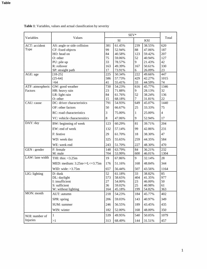
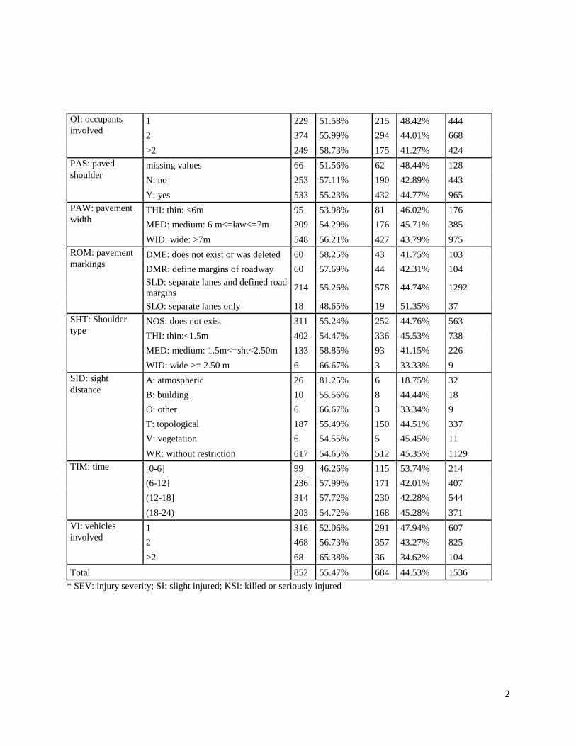
contained 1,536 records. Table 1 provides information on the data used for this study.

(insert Table 1)

3

Eighteen (18) variables were used with the class variable of injury severity (SEV) in an attempt to

identify the important variables that affect injury severity in traffic accidents.

The data contained information related to the accidents and other information related to the drivers.

The data included variables describing the conditions that contributed to the accident and injury

severity.

Injury severity variables: number of injuries (e.g., passengers, drivers and pedestrians),

severity level of injuries (e.g., slight injured –SI– and killed or seriously injured –KSI).

Following previous studies (Chang and Wang, 2006; Milton et al., 2008) the injury severity of

an accident is determined according to the level of injury to the worst injured occupant.

Roadway information: characteristics of the roadway on which the accidents occurred (e.g.,

pavement width, lane width, shoulder type, pavement markings, sight distance, if the shoulder

was paved or not, etc.)

Weather information: weather conditions when the accident occurred (e.g., good weather, rain,

fog, snow and windy)

Accident information: contributing circumstances (e.g., type of accident, time of accident

(hour, day, month and year), and vehicles involved in the accident).

Driver data: characteristics of the driver, such as age or gender

3. Method

The procedure used in this study has been the following:

1. The original dataset obtained from the DGT was divided into two subsets: a training set

containing 2/3 of the data (1,024 records), and a testing set containing the rest of the data (512

records). The testing set was used to validate the results obtained using the training set.

2. Based on the eighteen variables taken from the accident reports (see Table 1), identification of

the variables that affect injury severity in traffic accidents was performed using different

methods of evaluator-search algorithms.

3. For each one of the selected subsets of variables, ten simplified BNs were built using the hill

climbing search algorithm and the MDL score (De Oña et al., 2011).

4. The performance of the built BNs using the selected subsets of variables was compared with

the performance of the original BN which was built using the eighteen variables (BN-18).

Five performance evaluation indicators were used.

5. Of all the simplified built BNs, the selected ones are those whose results improve or maintain

the results obtained by the performance indicators of BN-18 in 90% of the cases or more, and

whose improvements are statistically significant.

6. For the selected BNs, the variables that repeat in more than 50% of the cases are identified and

a new BN is built using these variables.

7. Finally, the results obtained by this new BN, based on a double process of variable selection

procedure, are compared with those obtained by BN-18.

3.1. Variable selection methods

In machine learning, variable selection is a process that is used to select a subset of variables and to

remove variables that do not contribute to the performance of the machine learning technique used.

4

In this study, we used six evaluators with eleven search methods. Weka’s Select Variable Panel

(Witten and Frank, 2005) was used to perform the variable selection.

A brief description of each of the evaluators used is given below:

1. Correlation-based variable selection (CfsSubsetEval): this evaluator measures the predictive

ability of each variable individually and the degree of redundancy among them. It selects the

sets of variables that are highly correlated with the class but have low inter-correlation with

each other (Hall, 1998).

2. Consistency-based variable selection (ConsistencySubsetEval): this evaluator measures the

degree of consistency of the variable sets in class values when the training values are

projected onto the set. This evaluator is usually used in conjunction with a random or

exhaustive search (Liu and Setiono, 1996).

3. Classifier Subset Evaluator (ClassifierSubsetEval): this evaluator uses the classifier specified

in the object editor as a parameter, to evaluate sets of variables on the training data or on a

separate holdout set (Witten and Frank, 2005).

4. Wrapper Subset Evaluator (WrapperSubsetEval): this evaluator uses a classifier to evaluate

variable sets and it employs cross-validation to estimate the accuracy of the learning scheme

for each set (Khhavi and John, 1997).

5. Filtered Subset Evaluator (FilteredSubsetEval): The filter model evaluates the subset of

variables by examining the intrinsic characteristic of the data without involving any data

mining algorithm (Witten and Frank, 2005).

6. Cost Sensitive Subset Evaluator (CostSensitiveSubsetEval): This evaluator projects the

training set into attribute set and measure consistency in class values, making the subset cost

sensitive (Liu and Setiono, 1996).

A brief description of each of the search methods used is given below:

1. Best First: this Search method uses greedy hillclimbing augmented with a backtracking

facility to search through the variables’ subsets. Best first may start with an empty set of

variables and search forward, or start with a full set of variables and search backward, or start

at any point and search in both directions (Pearl, 1984).

2. Genetic Search: An initial population is formed by generating many individual solutions.

During each successive generation, a proportion of the existing population is selected to breed

a new generation. This process is repeated until increasing the average fitness, and reaching a

termination condition (Goldberg, 1989).

3. Greedy Stepwise: Performs a greedy forward or backward search through the space of

variables’ subsets. The search could be initiated with none or with all the variables or from an

arbitrary point in the space. Thus, the search is stopped when the addition or deletion of any

variables that remains; results in a decrease in evaluation (Russell and Norvig, 2003).

4. Linear Forward Selection: this search method is an extension of Best First where a fixed

number k of variables is selected, whereas k is increased in each step when fixed-width is

selected. The search direction can be forward or floating forward selection (with optional

backward search steps) (Gutlein et al., 2009).

5. Scatter Search V1: Starts with a population of many significant variables and stops when the

result is higher than a given threshold or when no further improvement could be attained

(García López et al.,2006).

6. Tabu Search: It explores the solution space beyond the local optimum, once a local optimum

is reached; upward moves and those worsening the solutions are allowed (Hedar, 2008).

5

7. Rank Search: Uses a variable/subset evaluator to rank all variables. If a subset evaluator is

specified then a forward selection search is used to generate a ranked list. From the ranked list

of variables, subsets of increasing size are evaluated (Witten and Frank, 2005).

8. Exhaustive Search: Performs an exhaustive search through the space of variables’ subsets

starting from the empty set of variables and reporting the best subset found (Witten and Frank,

2005).

9. Subset Size Forward Selection: Performs an interior cross-validation, where it is performeded

on each fold to determine the optimal subset-size. In the final step the search is performed on

the whole data (Gutlein et al., 2009).

10. Random Search: Performs a random search in the space of variables’ subsets. A random

search is started from a random point, if no initial point is chosen, and reports the best subset

found. If a start set is set, Random searches randomly for subsets that are as good as or better

than the start point with the same number of variables or with a lower number of variables

(Liu and Setiono, 1996).

11. Race Search: Races the cross validation error of competing subsets of variables, and is only

used with a ClassifierSubsetEval (Moore and Lee,1994).

3.2. Bayesian Networks definition

Over the last decade, BNs have become a popular representation for encoding uncertain expert

knowledge in expert systems. The field of BNs has grown enormously, with theoretical and

computational developments in many areas (Mittal et al., 2007) such as: modeling knowledge in

bioinformatics, medicine, document classification, information retrieval, image processing, data

fusion, decision support systems, engineering, gaming, and law.

Let U=x1, . . . , xn, n≥1 be a set of variables. A BN over a set of variables U is a network structure,

which is a Directed Acyclic Graph (DAG) over U and a set of probability tables Bp = p(xi|pa(xi), xi

U) where is the set of parents or antecedents of xi in BN and i=(1,2,3,….,n). A BN represents

joint probability distributions

Based on the theory of Bayesian networks (Neapolitan, 2004) the relations between variables,

represented by arcs in the graph, could represent causality, relevance or relations of direct dependence

between variables. In accordance with other authors (Acid et al., 2004), we do not assume a causal

intrpretation of the arcs in the networks, although in some cases this might be reasonable (other

approaches that explicitly try to detect causal influence are discussed in Glymour et al. (1999) and

Pearl (2000)). Instead, the arcs are interpreted as direct dependence relationships between the linked

variables, and the absence of arcs means the absence of direct dependence between variables, however

indirect dependence relationships between variables could exist.

The classification task consists in classifying a variable y = x0 called the class variable, given a set of

variables U = x1 . . . xn, called attribute variables. A classifier h : U → y is a function that maps an

instance of U to a value of y. The classifier is learned from a dataset D consisting of samples over (U,

y). The learning task consists of finding an appropriate BN given a data set D over U.

For each one of the variable subsets selected in the previous step, BNs were built using the training

dataset, the hill climbing search algorithm and the MDL score. The search algorithm and the score

were applied in this study mainly because they are fast and widely used, and also produce good results

in terms of network complexity and accuracy (Madden, 2009).

3.3. Performance Evaluation Indicators

6

In order to measure the performance of the BNs built for each one of the variable subsets with the

training data several indicators were used. The performance evaluation indicators used in this study

were accuracy, specificity, sensitivity, the harmonic mean of sensitivity and specificity (HMSS) and

the ROC area.

(1)

(2)

(3)

(4)

Where tSI is true slight injured cases, tKSI true killed or seriously injured cases, fSI false slight injured

cases, and fKSI false killed or seriously injured cases.

Accuracy (see Eq. 1) is proportion of instances that were correctly classified by the classifier.

Accuracy only gives information on the classifier’s general performance. In some cases the accuracy

might be high because the classifier is able to classify values that belonged to only one class correctly.

Because the dataset used herein had an imbalanced distribution of KSI and SI, the overall accuracy

alone is somewhat misleading. In order to assess the performance of the classifier, other measures

should be used along with the overall accuracy, such as the quantities presented in Eqs. (2-4).

Sensitivity represents the proportion of correctly predicted SI among all the observed SI. Specificity

represents the proportion of correctly predicted KSI among all the observed KSI (see Eqs. 2 and 3).

Another measure used to assess the performance of the BN built was the Harmonic Mean of

Sensitivity and Specificity (HMSS), which gives an equal weight of both sensitivity and specificity

(see Eq. 4).

However, there is a trade-off between sensitivity and specificity, meaning it is necessary to calculate

another evaluation method. Therefore, we used the area under a Receiver Operating Characteristic

(ROC) curve as a target performance method. What ROC curves represent is the true positive rate

(sensitivity) vs. the false positive rate (1-specificity). ROC curves are more useful as descriptors of

overall performance, reflected by the area under the curve, with a maximum of 1.00 describing a

perfect test and an ROC area of 0.50 describing a valueless test.

Finally, to validate the results, the measures described above are also calculated for each BN and the

testing dataset.

4. Results and Discussion

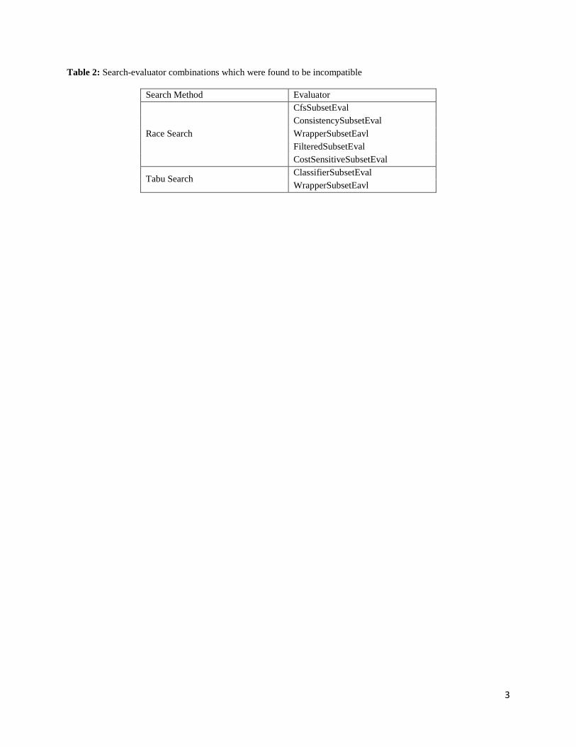
All the possible combinations of evaluator-search algorithms described in section 3.1 were applied (59

combinations). The total number of combinations was supposed to be 66; however, seven

combinations were found to be incompatible. Table 2 shows the unused combinations.

(insert table 2)

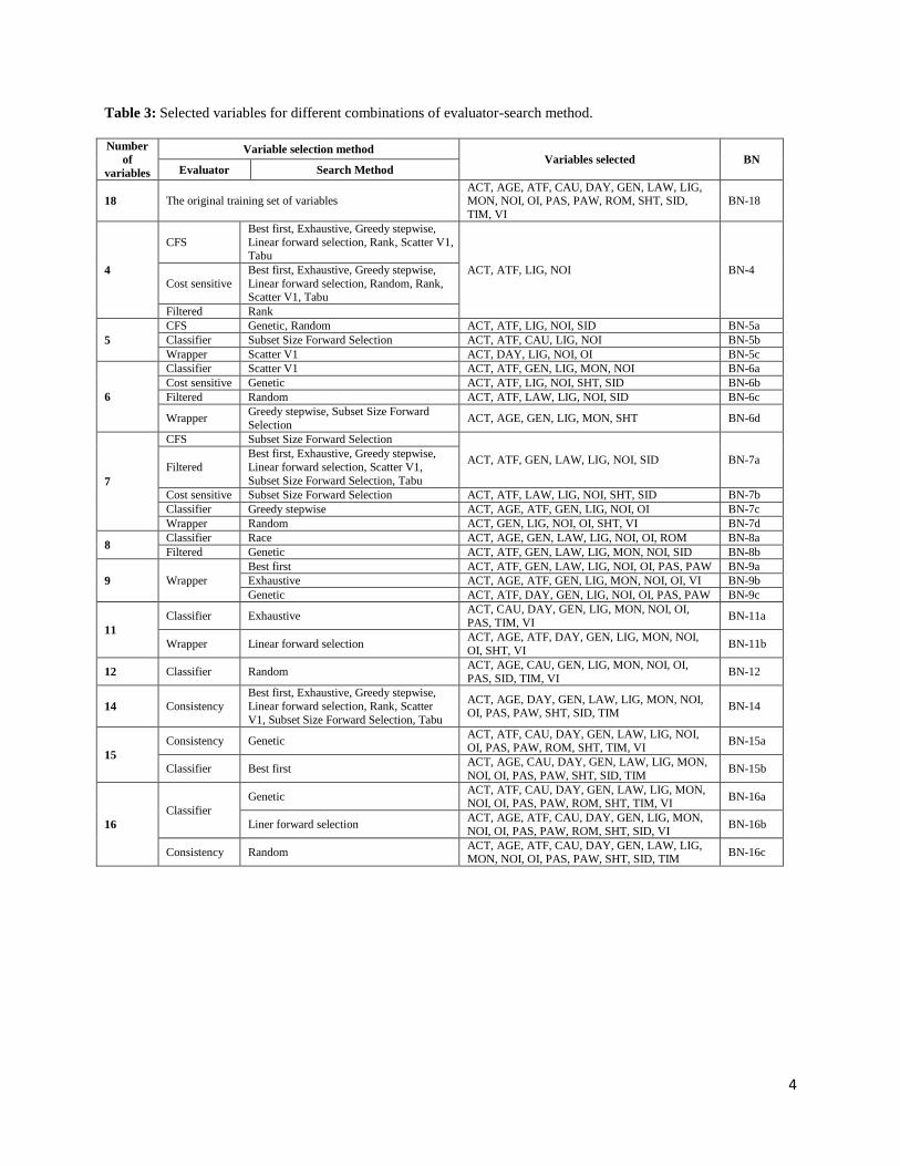
Table 3 shows the variables selected after running the 59 different combinations of the evaluator-

search algorithms. The number of selected variables lies between four variables (ACT, ATF, LIG and

NOI), as obtained using Correlation-based variable selection, Filtered Subset Evaluator and Cost

7

Sensitive Subset Evaluator with several search methods, and a maximum number of sixteen selected

variables.

(insert table 3)

The same subset of variables could be selected by several evaluator-search combinations. As an

example, one of the subset composed of four variables (ACT, ATF, LIG and NOI) is selected by

seventeen different combinations of evaluator-search algorithms.

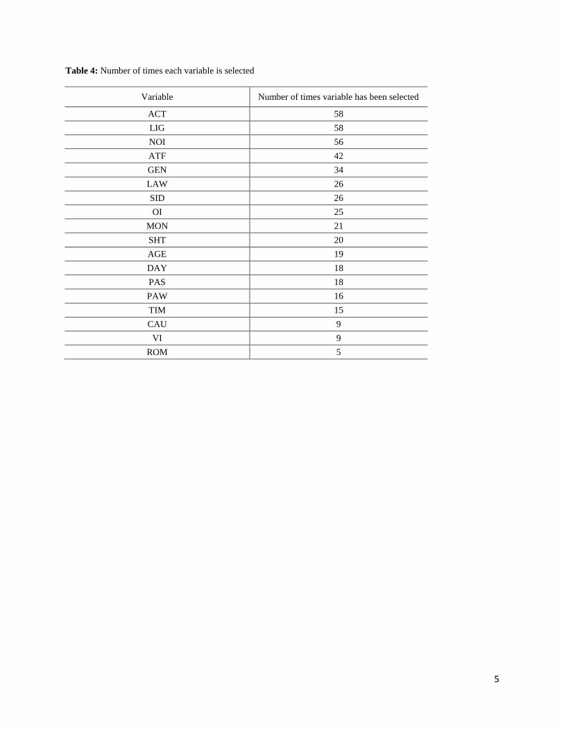
(insert table 4)

Table 4 shows the number of times that each one of the eighteen variables has been selected. There are

three variables that were selected approximately 95% of times. The variables ACT (accident type) and

LIG (lighting) were selected 58 times over 59 combinations, which mean that they were selected

almost by all the evaluator-search combinations. NOI (number of injuries) was the third most selected

variable (56 times). The forth most selected variable was ATF (atmospheric factors) with 42 times. On

the other hand, the least selected variable was ROM (pavement markings), with only 5 times.

For each subset of selected variables 20 BNs were built representing 10 runs for the training set, and

10 for the testing set, for each one of the selected variable groups (26 groups) and for the eighteen

original variables. In total, 540 BNs have been built for this analysis. The averages of the performance

evaluation indicators described in section 3.3 are calculated for each one of these BNs.

(insert table 5)

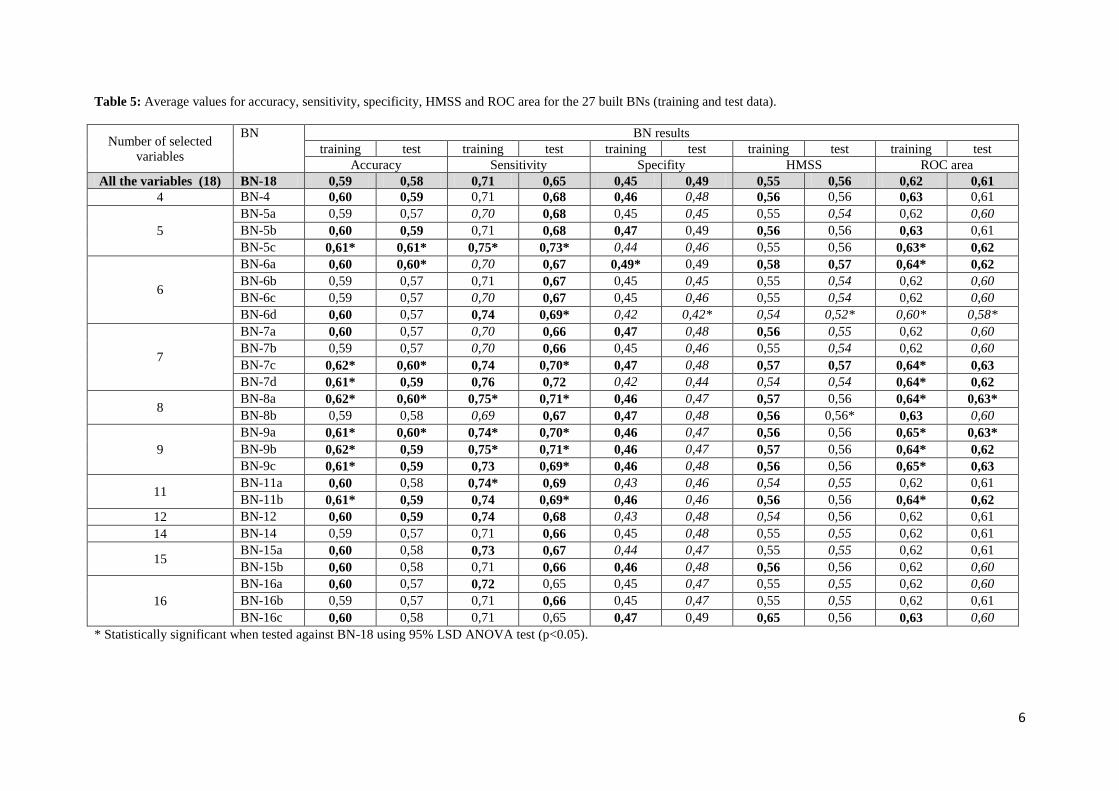
Table 5 shows the average results of these indicators for the 27 BNs for the training and the testing

sets of data. With respect to the results obtained by the training set, the following findings could be

highlighted:

The values obtained for the all the performance indicators lie in the range between 0.42 and

0.76. These values however, are in the range of values obtained by other researchers (Delen et

al., 2006; Abdelwahab and Abdel-Aty, 2001).

The highest values obtained for the indicators of Sensitivity and ROC area are 0.69-0.76 for

the former, and in the range of 0.60-0.65 for the latter.

The worst results were obtained for Specificity (between 0.42 and 0.49). This indicator is used

to measure the ability of the model to classify the KSI cases. Since the number of SI cases is

higher than the number of KSI cases, and thus the BNs are a data mining technique, better

results are obtained for larger groups (SI in this case) from those obtained for smaller groups

(Chang and Wang, 2006).

As Accuracy and HMSS are indicators that take into account both Sensitivity and Specificity,

their results are intermediate, ranging between 0.59 and 0.62 for Accuracy and 0.54 and 0.65

for HMSS.

In most of the cases (74%), the values of the performance indicators obtained for the simplified BNs

maintain or improve the results as compared to those of BN-18. Average values for each of the 27

BNs (training and testing sets) were tested for statistical significance (p<0.05) using least significant

difference (LSD) ANOVA test.

Table 5 shows 7 BNs (BN-6a, BN-7c, BN-8a, BN-9a, BN-9b, BN-9c and BN-11b) that present

statistically significant improvements in their performance indicators with respect to BN-18, with only

a worsened value in one of their indicators. Having a closer look at these 7 BNs (see Table 3) it is

8

observed that there are 7 variables (ACT, AGE, ATF, GEN, LIG, NOI, and OI) that repeat in more

than 50% of these 7 BNs.

None of the previously built BNs was formed using this set of variables; therefore, a new BN (BN-7)

was built using these 7 variables. Table 6 shows the average values of the indicators for this new BN.

The results of all the performance indicators of this BN improve with respect to BN-18 except for one

indicator (specificity for the test set), and these improvements are statistically significant (p<0.05) in

60% of the cases (accuracy, sensitivity and ROC area).

(insert Table 6)

Thus, it could be said that a simplified BN has been identified (BN-7), with only seven variables,

whose results are similar or even better than those obtained by the original BN (BN-18) which

includes all variables obtained from the police accidents report.

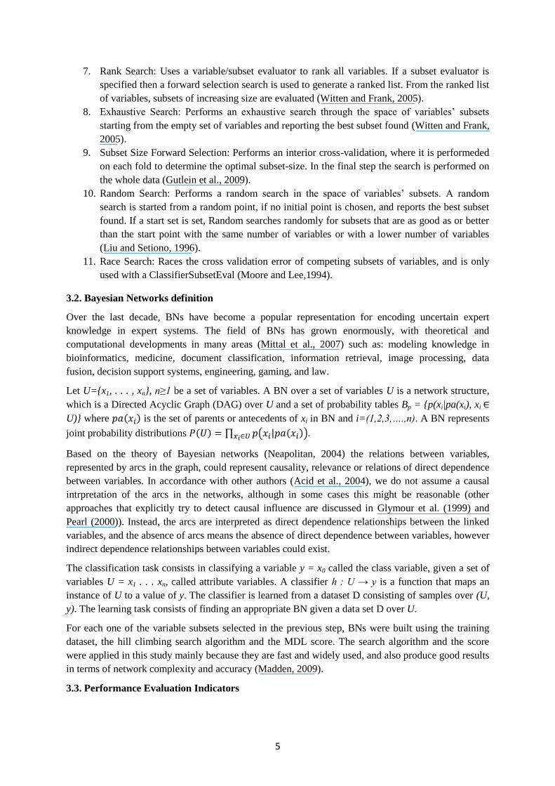
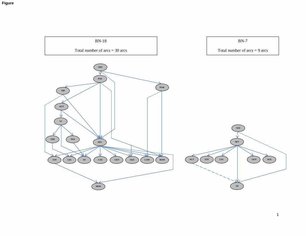
Figure 1 shows the structure of both BN-18 and BN-7. It shows that the complexity of the built BN is

relieved when built using the subset of seven variables. The indicator used to measure the complexity

of the built network is the number of arcs. The number of arcs was found to be 30 in the original BN

(BN-18), whereas it was decreased to 9 arcs for the network of BN-7. The arcs in the networks

indicate the existence of a relationship between variables. Where the arcs in a BN are not necessarily

causal, that is, a BN can satisfy the probability distribution of the variables in the BN without the arcs

being causal (Neapolitan, 2009). Thus, the arcs between variables in a non causal BN could imply a

sort of interrelationship(s) among these variables.

The structure of the BN-7 network is similar to the network structure built using the 18 variables (BN-

18), keeping in mind that 11 variables have disappeared in BN-7. Thus, the structure of relationships

between the variables SEV-ACT, SEV-LIG, SEV-GEN, SEV-OI, SEV-AGE, SEV-ATF, NOI-OI are

the same in both BN-18 and BN-7, except for the two new connections between SEV-NOI and ACT-

OI that appeared in BN-7.

The variables that appear in BN-7 (accident type, age, atmospheric factors, gender, lighting, number of

injuries and occupants involved) could be considered the ones that significantly affect the injury

severity in a traffic accident.

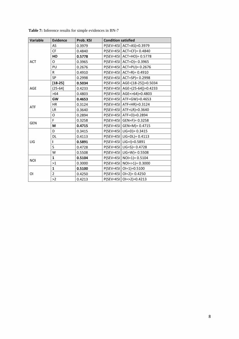
(insert Table 7)

Setting evidences for the variables in BN-7 could give indications of the values of variables that

contribute to the occurrence of a killed or seriously injured (KSI) individual in a traffic accident. Table

7 assists in the identification of the variables and values that contribute the most to the occurrence of a

KSI individual in a traffic accident. For each variable, the probability of a value was set to be 1

(setting simple evidence). Thus, the associated probability of severity was calculated.

Bold values in Table 7 highlight the highest probability values of a KSI for each variable. For

example, Table 7 shows that the highest probability of KSI occurs when the lighting is insufficient

(LIG=I). BN-7 allows predicting that the probability of having a KSI accident is 58.91% if LIG=I. For

the other six variables (ACT, AGE, ATF, GEN, NOI and OI), when information is only available

about the variable itself, the highest probability of SEV=KSI occurs in the case of: ACT=head on;

AGE=[18-25]; ATF=good weather; GEN=male; NOI=1; and OI=1.

Although some of these results could seem to be strange (for example, the probability of having KSI is

higher when NOI=1 or when OI=1, instead of increasing the severity as NOI or OI increases), they are

consistent with other results found in the literature:

9

Kockelman et al. (2002) found accident type to be one of the significant variables that affect

the injury severity of traffic accidents. They found that head on crashes were more dangerous

than angle crashes, left-side, and right-side crashes; they also found that they were significant

in accidents that involved killed or seriously injured.

Age was found to be a significant variable affecting the injury severity of traffic accidents by

Tavris et al. (2001). They also found that male drivers in the age group (16–24) years were

much more likely to be involved in killed or seriously injured accidents than those involving

older drivers.

Xie et al. (2009) found that adverse weather can actually lead to lower probability of suffering

the most severe category of injuries. They explained their results by the fact that under such

conditions, drivers tend to drive at lower speeds and be more cautious. They also found gender

to be a significant variable; their results indicated that the chance for male drivers to suffer the

most severe category of injuries is less than female drivers under the same crash

circumstances. Their results coincided with the results found by Kockelman et al. (2002).

Lighting has been found to be a significant variable defining injury severity in traffic accidents

in several studies (Abdel-Aty, 2003; Helay et al., 2007 and Gray et al., 2008). They have

found that more severe injuries are predicted during darkness.

Scheetz et al. (2009) found that the number of injured occupants was a significant factor in

classifying injury severity.

Occupant involved in a traffic accident was found to be a significant variable by Dupont et al.

(2010). They found that the higher the number of vehicles involved in the accident and the

level of occupancy of these vehicles, the higher the probability for each car occupant to

survive.

However, relationships between the variables and injury severity in traffic accidents are more subtle.

The effect of variable’s value does not always lead to the same outcome (e.g. not always that OI

decreases the probability of KSI decreases). Simplified BN allow and facilitate analyzing these

subtleties. For example, Table 7 shows that, in general, the probability of a KSI accident decreases

with the number of OI:

P(SEV=KSI OI=1)=51.00%

P(SEV=KSI OI=2)=42.50%

P(SEV=KSI OI=>2)=42.13%

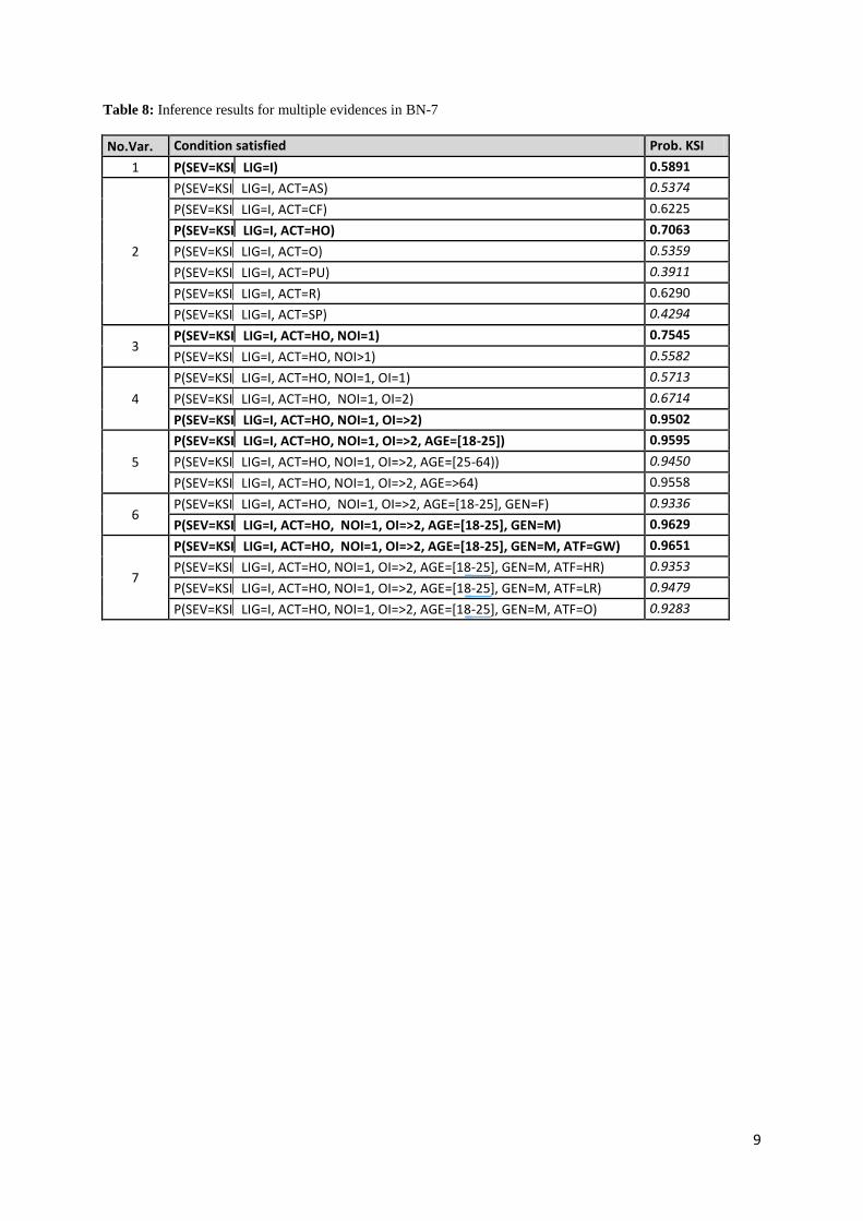
However, Table 8 shows that the probability of SEV=KSI in the case of HO accidents that occurred in

conditions of insufficient lighting (LIG=I) and with only one injury (NOI=1) increases with the

number of OI:

P(SEV=KSI LIG=I, ACT=HO, NOI=1, OI=1)=57.13%

P(SEV=KSI LIG=I, ACT=HO, NOI=1, OI=2)=67.14%

P(SEV=KSI LIG=I, ACT=HO, NOI=1, OI=>2)=95.02%

10

(insert Table 8)

Table 7 shows the probability of having an accident with SEV=KSI when knowing a priori the value

of only one variable (simple evidences). Table 8 shows the probability of KSI when knowing a priori

the value of more than one variable (multiple evidences). Based on the case that presents the highest

probability in Table 7 (LIG=I), the probabilities with multiple evidences were calculated in a

descending order (ACT, NOI, OI, AGE, GEN and ATF) (see Table 8). In each step, the highest

probability value was selected and used for the next step.

Simplified BN allow this kind of analysis with multiple evidences. This analysis provides added value

information with regard to the analysis with simple evidences. For example, Table 7 shows that the

probability of an accident with SEV=KSI is 51% in the case of NOI=1 and 30% in the case of NOI>1.

However, in HO accidents under insufficient lighting (ACT=HO and LIG=I) the probability of

SEV=KSI increases to 75.45% for NOI=1 and becomes 55.82% for NOI>1. Table 8 also shows that an

accident with LIG=I, ACT=HO, NOI=1, OI>2, AGE=[18-25], GEN=M and ATF=GW has a

probability of 96.51% of having SEV=KSI.

5. Summary and conclusions

The main objective of this research work was to determine if it is possible to maintain or improve the

performance of a model that is used to predict the injury severity of a traffic accident based on BNs

reducing the number of variables considered in the analysis. The performance of the model was

measured using five indicators (accuracy, specificity, sensitivity, HMSS and ROC area).

In order to perform this analysis 1,536 records of traffic accidents on rural highways with information

about 18 variables that are related with the severity of the accidents based on the standard police

reports used in Spain were used. 59 combinations of evaluator-search algorithms, which are

commonly used in data mining, were used and 26 subsets of variables were identified.

Within these subsets of variables the variable accident type (ACT), lighting (LIG) and number of

injuries (NOI) were selected the most times (over 95%). Therefore, it could be said that these variables

are the most significant ones in the classification of injury severity in traffic accidents, since they are

included in almost all the selected subsets of variables.

For each one of these subsets of variables, 10 simplified BNs were built for the training stage and

another 10 for the testing stage. In total, 540 BNs were built using the hill climbing search algorithm

and the MDL score (de Oña et al., 2011).

Comparing the average values of the indicators for each one of the simplified BNs with respect to the

average values obtained for the original BN (BN-18), it is observed that, in most of cases (74%), the

performance indicators values for the simplified BNs maintained or improved in comparison with

those of BN-18. Therefore, it could be said that, in most cases, simplified networks maintain the

performance of the original BN.

Seven BNs were found to present statistically significant improvements in their performance

indicators with respect to BN-18 and only one value of these indicators get worsened. In more than

50% of these BNs the following variables are repeated: ACT, AGE, ATF, GEN, LIG, NOI and OI.

These 7 variables were used to built a new BN (BN-7). The results of the performance indicators of

this BN with respect to BN-18 improve practically in all the cases, and these improvements are

statistically significant (p<0.05) in 60% of the cases (accuracy, sensitivity and ROC area).

11

Therefore, this research work shows that, for the analysis of the severity of road accidents by Bayesian

networks on rural roads, it is possible to reduce the number of variables considered in more than 60%

(from 18 to 7 variables) maintaining the performance of the models and reducing their complexity.

Thus the findings of this research work agrees with Chang and Wang (2006) where they stated that if a

model is applied only on a few important variables, more useful results could be obtained.

The procedure used to simplify BN models to analyze the severity of traffic accidents on rural

highways could be also applied to other types of infrastructure (intersections, freeways, etc.) as well as

to other models used to assess severity of traffic accidents (multinomial logit models, hierarchical logit

models, probit models, etc.).

Acknowledgements

Support from Spanish Ministry of Science and Innovation (Research Project TRA2007-63564) as well

as the data provided by the Spanish General Directorate of Traffic (DGT) are gratefully

acknowledged.

References

1. Abdel-Aty, M. (2003). Analysis of driver injury severity levels at multiple locations using ordered

probit models. Journal of Safety Research, 34, 597–603.

2. Abdelwahab, H.T., & Abdel-Aty M.A. (2001). Development of Artificial Neural Network Models

to Predict Driver Injury Severity in Traffic Accidents at Signalized Intersections. Transportation

Research Record, 1746, 6-13.

3. Acid, S., de Campos, L.M., Fernández-Luna, J.M., Rodríguez, S., J.M., R. & Salcedo, J.L. (2004)

'A comparison of Learning algorithms for Bayesian networks: a case study based on data from an

emergency medical service, Artificial Intelligence in Medicine, 30, 215-232

4. Al-Ghamdi, A.S. (2002). Using logistic regression to estimate the influence of accident factors on

accident severity, Accident Analysis and Prevention, 34, 729–741.

5. Bédard M., Guyatt, G.H., Stones, M.J., & Hirdes, J.P. (2002). The independent contribution of

driver, crash, and vehicle characteristics to driver fatalities, Accident Analysis and Prevention, 34,

717–727.

6. Chang, L.Y, & Wang, H.W. (2006). Analysis of traffic injury severity: An application of non-

parametric classification tree techniques. Accident Analysis and Prevention, 38, 1019-1027.

7. Chen, W.H, & Jovanis, P.P. (2000). Method for identifying factors contributing to driver-injury

severity in traffic crashes. Transportation Research Record, 1717, 1-9.

8. De Oña, J., Mujalli, R.O., & Calvo, F. (2011). Analysis of traffic accident injury severity on

Spanish rural highways using Bayesian networks. Accident Analysis and Prevention, 43 (1), 402-

411.

9. Delen, D., Sharda, R., & Bessonov, M. (2006). Identifying significant predictors of injury severity

in traffic accidents using a series of artificial neural networks. Accident Analysis and Prevention,

38, 434–444.

10. Dirección General de Tráfico – DGT. (2007). Anuario Estadístico 2007, NIPO: 128-08-161-7,

Retrieved from http://www.dgt.es/.

11. Dupont, E., Martensen, H., Papadimitriou, E., & Yannis, G. (2010). Risk and Protection factors in

fatal accidents. Accident Analysis and Prevention, 42, 645-653.

12. García López, F., García Torres, M., Melián Batista, B., Moreno Pérez, J., & Moreno-Vega, J.

(2006). Solving feature subset selection problem by a Parallel Scatter Search . European Journal

of Operational Research , 477-489.

13. Gray, R.C., Quddus, M.A. & Evans, A. (2008). Injury severity analysis of accidents involv- ing

young male drivers in Great Britain. Journal of Safety Research, 39, 483–495.

14. Glymour, C., Cooper, G. & Chickering, D.M. (ed.) (1999). Computation Causation and

Discovery, The AAAI Press.

15. Goldberg, D. (1989). Genetic algorithms in search, optimization and machine learning. Addison-

Wesley.

12

16. Gutlein, M., Frank, E., Hall, M., & Karwath, A. (2009). Large scale attribute selection using

wrappers. - Proceedings of 2009 IEEE Symposium on Computational Intelligence and Data

Mining, CIDM 2009, Washington.

17. Hall, M. (1998). Correlaion-based Feature Subset Selection for Machine Learning. Hamilton,

New Zeland (Doctoral Dissertation).

18. Hedar, A.-R. W. (2008). Tabu search for attribute reduction in rough set theory. Soft Computing ,

12 (9) 909-918.

19. Helai, H., Chor, C.H., & Haque, M.M. (2008). Severity of driver injury and vehicle dam- age in

traffic crashes at intersections: a Bayesian hierarchical analysis. Accident Analysis and Prevention,

40, 45–54.

20. Khhavi, R., & John, G. (1997). Wrappers for feature subset selection. Artificial Intelligence, 97,

273-324.

21. Kockelman, K.M., & Kweon, Y.J. (2002). Driver injury severity: an application of ordered probit

models. Accident Analysis and Prevention, 34, 313–321.

22. Kopelias, P., Papadimitriou, F, Papandreou, K, & Prevedouros, P. (2007). Urban Freeway Crash

Analysis. Transportation Research Record: Journal Transportation Research Board, 2015, 123-

131.

23. Liu, H., & Setiono, R. (1996). A probabilistic approach to feature selection- A filter solution.

Proceedings of 13th International Conference on Machine Learning.

24. Madden, M. G. (2009). On the classification performance of TAN and general Bayesian networks.

Journal of Knowledge-Based Systems, 22, 489-495.

25. Milton, J.C., Shankar, V.N., & Mannering, F.L. (2008). Highway accident severities and the

mixed logit model: An exploratory empirical analysis. Accident Analysis and Prevention, 40, 260–

266.

26. Mittal, A., Kassim, A., & Tan, T. (2007). Bayesian network technologies: Applications and

graphical models. IGI Publishing.

27. Moore, A., & Lee, M. (1994). Efficient algorithms for minimizing cross validation error.

Proceedings of 11th International Conference on Machine Lerning.

28. Neapolitan, R.E. (2004). Learning Bayesian Networks, Prentice Hall.

29. Neapolitan, R.E. (2009). Probabilistic Methods for Bioinformatics. San Francisco, California:

Morgan Kaufmann Publishers.

30. Pearl, J. (1984). Heuristics: Intelligent search strategies for computer problem solving. Addison-

Wesley.

31. Pearl J. (2000). Causality: Models, Reasoning and Inference. Cambridge: Cambridge University

Press.

32. Russell, S., & Norvig, P. (2003). Artificial Intelligence: A modern approach . Upper Saddle River,

New Jersey: Prentice Hall.

33. Scheetz, L.J., Zhang, J., & Kolassa, J. (2003). Classification tree to identify severe and moderate

injuries in young and middle aged adults. Artificial Intelligence in Medicine, 45, 1–10.

34. Simoncic, M. (2004). A Bayesian network model of two-car accidents. Journal of transportation

and Statistics, 7, 13-25.

35. Tavris, D.R., Kuhn, E.M., & Layde, P.M. (2001). Age and gender patterns in motor vehicle crash

injuries: importance of type of crash and occupant role. Accident Analysis and Prevention, 33,

167–172.

36. Witten, I. H., & Frank, E. (2005). Data Mining: Practical Machine Learning Tools and

Techniques (2nd

Edition). San Francisco, California: Morgan Kaufmann Publishers.

37. Xie, Y., Zhang, Y., & Liang, F. (2009). Crash Injury Severity Analysis Using Bayesian Ordered

Probit Models. Journal of Transportation Engineering ASCE, 135 (1),18-25.

38. Yamamoto, T., & Shankar, V.N. (2004). Bivariate ordered-response probit model of driver’s and

passenger’s injury severities in collisions with fixed objects. Accident Analysis and Prevention,

36, 869–876.

39. Yau, K.K.W., Lo, H.P., & Fung, S.H.H. (2006). Multiple-vehicle traffic accidents in Hong Kong,

Accident Analysis and Prevention, 38,1157–1161.

13

List of Figures:

Figure 1: BN structure for BN-18 and BN-7.

List of Tables:

Table 1: Variables, values and actual classification by severity

Table 2: Search-evaluator combinations which were found to be incompatible

Table 3: Selected variables for different combinations of evaluator-search method

Table 4: Number of times each variable is selected

Table 5: Average values for accuracy, sensitivity, specificity, HMSS and ROC area for the 27 built

BNs (training and test data).

Table 6: Average values for accuracy, sensitivity, specificity, HMSS and ROC area for BN-18 and

BN-7 (training and test data).

Table 7: Inference results for simple evidences in BN-7

Table 8: Inference results for multiple evidences in BN-7

VITAE

Juan de Oña is an Associate Professor in the Department of Civil Engineering at the University

of Granada. M.Eng. in Civil Engineering (1996), Ecole Nationale de Ponts et Chaussées, Paris

(France). M.Sc. in Transportation (1999), Polytechnic University of Madrid (Spain). He holds a

Ph.D. in Transportation Engineering (2001) from the University of Granada. He is the Director

of the Transportation and Safety Research Group, Secretariat-General of Universities, Research

and Technology of Andalucía. His current fields of interest include road safety, transport

planning and management, and railways management.

Randa Oqab Mujalli is a PhD student in the Department of Civil Engineering at the University

of Granada. She holds both a BSc in Civil Engineering (2005) and an MSc in Transportation

Engineering (2007) from Jordan University of Science and Technology, Irbid (Jordan). She is

currently a Research Assistant in the Division of Transportation at the University of Granada,

Granada (Spain). Her fields of interest include traffic safety, transportation planning and

management, highway design, and Artificial intelligence and soft computing applications in

transportation engineering.

*Biographical sketch of all authors

1

BN-18

Total number of arcs = 30 arcs

BN-7

Total number of arcs = 9 arcs

PAS

SHT

PAW

SID

TIM

ROM LAW CAU

ACT

VI

NOI

MON

ATF OI LIG

SEV

AGE GEN

NOI

OI

ACT LIG ATF

SEV

AGE GEN

Figure

1

Table 1: Variables, values and actual classification by severity

Variables Values SEV*

Total

SI

KSI

ACT: accident AS: angle or side collision 381 61.45% 239 38.55% 620

Type CF: fixed objects 99 52.94% 88 47.06% 187

HO: head on 84 40.58% 123 59.42% 207

O: other 75 59.06% 52 40.94% 127

PU: pile up 33 78.57% 9 21.43% 42

R: rollover 163 49.39% 167 50.61% 330

SP: straight path 17 73.91% 6 26.09% 23

AGE: age [18-25] 225 50.34% 222 49.66% 447

(25-64] 586 57.73% 429 42.27% 1015

>64 41 55.41% 33 44.59% 74

ATF: atmospheric GW: good weather 730 54.23% 616 45.77% 1346

Factors HR: heavy rain 23 71.88% 9 28.13% 32

LR: light rain 84 61.76% 52 38.24% 136

O: other 15 68.18% 7 31.81% 22

CAU: cause DC: driver characteristics 791 54.93% 649 45.07% 1440

OF: other factors 50 66.67% 25 33.33% 75

RC: road characteristics 3 75.00% 1 25.00% 4

VC: vehicle charactersitics 8 47.06% 9 52.94% 17

DAY: day BW: beginning of week 123 60.29% 81 39.71% 204

EW: end of week 132 57.14% 99 42.86% 231

F: festive 29 61.70% 18 38.30% 47

WD: week day 325 55.65% 259 44.35% 584

WE: week end 243 51.70% 227 48.30% 470

GEN : gender F: female 148 63.79% 84 36.21% 232

M: male 704 53.99% 600 46.01% 1304

LAW: lane width THI: thin: <3.25m 19 67.86% 9 32.14% 28

MED: medium: 3.25m<=L<=3.75m 176 51.16% 168 48.84% 344

WID: wide: >3.75m 657 56.44% 507 43.56% 1164

LIG: lighting D: dusk 52 61.18% 33 38.82% 85

DL: daylight 573 58.65% 404 41.35% 977

I: insufficient 27 54.00% 23 46.00% 50

S: sufficient 36 59.02% 25 40.98% 61

W: without lighting 164 45.18% 199 54.82% 363

MON: month AUT: autumn 218 54.23% 184 45.77% 402

SPR: spring 206 59.03% 143 40.97% 349

SUM: summer 246 56.55% 189 43.45% 435

WIN: winter 182 52.00% 168 48.00% 350

NOI: number of 1 539 49.95% 540 50.05% 1079

Injuries >1 313 68.49% 144 31.51% 457

Table

2

OI: occupants 1 229 51.58% 215 48.42% 444

involved 2 374 55.99% 294 44.01% 668

>2 249 58.73% 175 41.27% 424

PAS: paved missing values 66 51.56% 62 48.44% 128

shoulder N: no 253 57.11% 190 42.89% 443

Y: yes 533 55.23% 432 44.77% 965

PAW: pavement THI: thin: <6m 95 53.98% 81 46.02% 176

width MED: medium: 6 m<=law<=7m 209 54.29% 176 45.71% 385

WID: wide: >7m 548 56.21% 427 43.79% 975

ROM: pavement DME: does not exist or was deleted 60 58.25% 43 41.75% 103

markings DMR: define margins of roadway 60 57.69% 44 42.31% 104

SLD: separate lanes and defined road 714 55.26% 578 44.74% 1292

margins

SLO: separate lanes only 18 48.65% 19 51.35% 37

SHT: Shoulder NOS: does not exist 311 55.24% 252 44.76% 563

type THI: thin:<1.5m 402 54.47% 336 45.53% 738

MED: medium: 1.5m<=sht<2.50m 133 58.85% 93 41.15% 226

WID: wide >= 2.50 m 6 66.67% 3 33.33% 9

SID: sight A: atmospheric 26 81.25% 6 18.75% 32

distance B: building 10 55.56% 8 44.44% 18

O: other 6 66.67% 3 33.34% 9

T: topological 187 55.49% 150 44.51% 337

V: vegetation 6 54.55% 5 45.45% 11

WR: without restriction 617 54.65% 512 45.35% 1129

TIM: time [0-6] 99 46.26% 115 53.74% 214

(6-12] 236 57.99% 171 42.01% 407

(12-18] 314 57.72% 230 42.28% 544

(18-24) 203 54.72% 168 45.28% 371

VI: vehicles 1 316 52.06% 291 47.94% 607

involved 2 468 56.73% 357 43.27% 825

>2 68 65.38% 36 34.62% 104

Total 852 55.47% 684 44.53% 1536

* SEV: injury severity; SI: slight injured; KSI: killed or seriously injured

3

Table 2: Search-evaluator combinations which were found to be incompatible

Search Method Evaluator

Race Search

CfsSubsetEval

ConsistencySubsetEval

WrapperSubsetEavl

FilteredSubsetEval

CostSensitiveSubsetEval

Tabu Search ClassifierSubsetEval

WrapperSubsetEavl

4

Table 3: Selected variables for different combinations of evaluator-search method.

Number

of

variables

Variable selection method Variables selected BN

Evaluator Search Method

18 The original training set of variables ACT, AGE, ATF, CAU, DAY, GEN, LAW, LIG, MON, NOI, OI, PAS, PAW, ROM, SHT, SID,

TIM, VI

BN-18

4

CFS

Best first, Exhaustive, Greedy stepwise,

Linear forward selection, Rank, Scatter V1, Tabu

ACT, ATF, LIG, NOI BN-4

Cost sensitive

Best first, Exhaustive, Greedy stepwise,

Linear forward selection, Random, Rank, Scatter V1, Tabu

Filtered Rank

5

CFS Genetic, Random ACT, ATF, LIG, NOI, SID BN-5a

Classifier Subset Size Forward Selection ACT, ATF, CAU, LIG, NOI BN-5b

Wrapper Scatter V1 ACT, DAY, LIG, NOI, OI BN-5c

6

Classifier Scatter V1 ACT, ATF, GEN, LIG, MON, NOI BN-6a

Cost sensitive Genetic ACT, ATF, LIG, NOI, SHT, SID BN-6b

Filtered Random ACT, ATF, LAW, LIG, NOI, SID BN-6c

Wrapper Greedy stepwise, Subset Size Forward

Selection ACT, AGE, GEN, LIG, MON, SHT BN-6d

7

CFS Subset Size Forward Selection

ACT, ATF, GEN, LAW, LIG, NOI, SID BN-7a Filtered

Best first, Exhaustive, Greedy stepwise,

Linear forward selection, Scatter V1,

Subset Size Forward Selection, Tabu

Cost sensitive Subset Size Forward Selection ACT, ATF, LAW, LIG, NOI, SHT, SID BN-7b

Classifier Greedy stepwise ACT, AGE, ATF, GEN, LIG, NOI, OI BN-7c

Wrapper Random ACT, GEN, LIG, NOI, OI, SHT, VI BN-7d

8 Classifier Race ACT, AGE, GEN, LAW, LIG, NOI, OI, ROM BN-8a

Filtered Genetic ACT, ATF, GEN, LAW, LIG, MON, NOI, SID BN-8b

9 Wrapper

Best first ACT, ATF, GEN, LAW, LIG, NOI, OI, PAS, PAW BN-9a

Exhaustive ACT, AGE, ATF, GEN, LIG, MON, NOI, OI, VI BN-9b

Genetic ACT, ATF, DAY, GEN, LIG, NOI, OI, PAS, PAW BN-9c

11

Classifier Exhaustive ACT, CAU, DAY, GEN, LIG, MON, NOI, OI,

PAS, TIM, VI BN-11a

Wrapper Linear forward selection ACT, AGE, ATF, DAY, GEN, LIG, MON, NOI,

OI, SHT, VI BN-11b

12 Classifier Random ACT, AGE, CAU, GEN, LIG, MON, NOI, OI,

PAS, SID, TIM, VI BN-12

14 Consistency

Best first, Exhaustive, Greedy stepwise,

Linear forward selection, Rank, Scatter

V1, Subset Size Forward Selection, Tabu

ACT, AGE, DAY, GEN, LAW, LIG, MON, NOI, OI, PAS, PAW, SHT, SID, TIM

BN-14

15

Consistency Genetic ACT, ATF, CAU, DAY, GEN, LAW, LIG, NOI, OI, PAS, PAW, ROM, SHT, TIM, VI

BN-15a

Classifier Best first ACT, AGE, CAU, DAY, GEN, LAW, LIG, MON,

NOI, OI, PAS, PAW, SHT, SID, TIM BN-15b

16

Classifier

Genetic ACT, ATF, CAU, DAY, GEN, LAW, LIG, MON, NOI, OI, PAS, PAW, ROM, SHT, TIM, VI

BN-16a

Liner forward selection ACT, AGE, ATF, CAU, DAY, GEN, LIG, MON,

NOI, OI, PAS, PAW, ROM, SHT, SID, VI BN-16b

Consistency Random ACT, AGE, ATF, CAU, DAY, GEN, LAW, LIG, MON, NOI, OI, PAS, PAW, SHT, SID, TIM

BN-16c

5

Table 4: Number of times each variable is selected

Variable Number of times variable has been selected

ACT 58

LIG 58

NOI 56

ATF 42

GEN 34

LAW 26

SID 26

OI 25

MON 21

SHT 20

AGE 19

DAY 18

PAS 18

PAW 16

TIM 15

CAU 9

VI 9

ROM 5

6

Table 5: Average values for accuracy, sensitivity, specificity, HMSS and ROC area for the 27 built BNs (training and test data).

Number of selected

variables

BN BN results

training test training test training test training test training test

Accuracy Sensitivity Specifity HMSS ROC area

All the variables (18) BN-18 0,59 0,58 0,71 0,65 0,45 0,49 0,55 0,56 0,62 0,61

4 BN-4 0,60 0,59 0,71 0,68 0,46 0,48 0,56 0,56 0,63 0,61

5

BN-5a 0,59 0,57 0,70 0,68 0,45 0,45 0,55 0,54 0,62 0,60

BN-5b 0,60 0,59 0,71 0,68 0,47 0,49 0,56 0,56 0,63 0,61

BN-5c 0,61* 0,61* 0,75* 0,73* 0,44 0,46 0,55 0,56 0,63* 0,62

6

BN-6a 0,60 0,60* 0,70 0,67 0,49* 0,49 0,58 0,57 0,64* 0,62

BN-6b 0,59 0,57 0,71 0,67 0,45 0,45 0,55 0,54 0,62 0,60

BN-6c 0,59 0,57 0,70 0,67 0,45 0,46 0,55 0,54 0,62 0,60

BN-6d 0,60 0,57 0,74 0,69* 0,42 0,42* 0,54 0,52* 0,60* 0,58*

7

BN-7a 0,60 0,57 0,70 0,66 0,47 0,48 0,56 0,55 0,62 0,60

BN-7b 0,59 0,57 0,70 0,66 0,45 0,46 0,55 0,54 0,62 0,60

BN-7c 0,62* 0,60* 0,74 0,70* 0,47 0,48 0,57 0,57 0,64* 0,63

BN-7d 0,61* 0,59 0,76 0,72 0,42 0,44 0,54 0,54 0,64* 0,62

8 BN-8a 0,62* 0,60* 0,75* 0,71* 0,46 0,47 0,57 0,56 0,64* 0,63*

BN-8b 0,59 0,58 0,69 0,67 0,47 0,48 0,56 0,56* 0,63 0,60

9

BN-9a 0,61* 0,60* 0,74* 0,70* 0,46 0,47 0,56 0,56 0,65* 0,63*

BN-9b 0,62* 0,59 0,75* 0,71* 0,46 0,47 0,57 0,56 0,64* 0,62

BN-9c 0,61* 0,59 0,73 0,69* 0,46 0,48 0,56 0,56 0,65* 0,63

11 BN-11a 0,60 0,58 0,74* 0,69 0,43 0,46 0,54 0,55 0,62 0,61

BN-11b 0,61* 0,59 0,74 0,69* 0,46 0,46 0,56 0,56 0,64* 0,62

12 BN-12 0,60 0,59 0,74 0,68 0,43 0,48 0,54 0,56 0,62 0,61

14 BN-14 0,59 0,57 0,71 0,66 0,45 0,48 0,55 0,55 0,62 0,61

15 BN-15a 0,60 0,58 0,73 0,67 0,44 0,47 0,55 0,55 0,62 0,61

BN-15b 0,60 0,58 0,71 0,66 0,46 0,48 0,56 0,56 0,62 0,60

16

BN-16a 0,60 0,57 0,72 0,65 0,45 0,47 0,55 0,55 0,62 0,60

BN-16b 0,59 0,57 0,71 0,66 0,45 0,47 0,55 0,55 0,62 0,61

BN-16c 0,60 0,58 0,71 0,65 0,47 0,49 0,65 0,56 0,63 0,60

* Statistically significant when tested against BN-18 using 95% LSD ANOVA test (p<0.05).

7

Table 6: Average values for accuracy, sensitivity, specificity, HMSS and ROC area for BN-18 and BN-7

(training and test data).

Indicators

BN results

BN-18 BN-7

training test training test

Accuracy 0,59 0,58 0,61* 0,60*

Sensitivity 0,71 0,65 0,74* 0,70*

Specificity 0,45 0,49 0,46 0,48

HMSS 0,55 0,56 0,57 0,57

ROC area 0,62 0,61 0,65* 0,63*

* Statistically significant when tested against BN-18 using 95% LSD ANOVA test (p<0.05).

8

Table 7: Inference results for simple evidences in BN-7

Variable Evidence Prob. KSI Condition satisfied

ACT

AS 0.3979 P(SEV=KSIACT=AS)=0.3979

CF 0.4840 P(SEV=KSIACT=CF)= 0.4840

HO 0.5778 P(SEV=KSIACT=HO)= 0.5778

O 0.3965 P(SEV=KSIACT=O)= 0.3965

PU 0.2676 P(SEV=KSIACT=PU)= 0.2676

R 0.4910 P(SEV=KSIACT=R)= 0.4910

SP 0.2998 P(SEV=KSIACT=SP)= 0.2998

AGE

[18-25] 0.5034 P(SEV=KSIAGE=[18-25])=0.5034

(25-64] 0.4233 P(SEV=KSIAGE=(25-64])=0.4233

>64 0.4803 P(SEV=KSIAGE=>64)=0.4803

ATF

GW 0.4653 P(SEV=KSIATF=GW)=0.4653

HR 0.3124 P(SEV=KSIATF=HR)=0.3124

LR 0.3640 P(SEV=KSIATF=LR)=0.3640

O 0.2894 P(SEV=KSIATF=O)=0.2894

GEN F 0.3258 P(SEV=KSIGEN=F)= 0.3258

M 0.4715 P(SEV=KSIGEN=M)= 0.4715

LIG

D 0.3415 P(SEV=KSILIG=D)= 0.3415

DL 0.4113 P(SEV=KSILIG=DL)= 0.4113

I 0.5891 P(SEV=KSILIG=I)=0.5891

S 0.4728 P(SEV=KSILIG=S)= 0.4728

W 0.5508 P(SEV=KSILIG=W)= 0.5508

NOI 1 0.5104 P(SEV=KSINOI=1)= 0.5104

>1 0.3000 P(SEV=KSINOI=>1)= 0.3000

OI

1 0.5100 P(SEV=KSIOI=1)=0.5100

2 0.4250 P(SEV=KSIOI=2)= 0.4250

>2 0.4213 P(SEV=KSIOI=>2)=0.4213

9

Table 8: Inference results for multiple evidences in BN-7

No.Var. Condition satisfied Prob. KSI

1 P(SEV=KSILIG=I) 0.5891

2

P(SEV=KSILIG=I, ACT=AS) 0.5374

P(SEV=KSILIG=I, ACT=CF) 0.6225

P(SEV=KSILIG=I, ACT=HO) 0.7063

P(SEV=KSILIG=I, ACT=O) 0.5359

P(SEV=KSILIG=I, ACT=PU) 0.3911

P(SEV=KSILIG=I, ACT=R) 0.6290

P(SEV=KSILIG=I, ACT=SP) 0.4294

3 P(SEV=KSILIG=I, ACT=HO, NOI=1) 0.7545

P(SEV=KSILIG=I, ACT=HO, NOI>1) 0.5582

4

P(SEV=KSILIG=I, ACT=HO, NOI=1, OI=1) 0.5713

P(SEV=KSILIG=I, ACT=HO, NOI=1, OI=2) 0.6714

P(SEV=KSILIG=I, ACT=HO, NOI=1, OI=>2) 0.9502

5

P(SEV=KSILIG=I, ACT=HO, NOI=1, OI=>2, AGE=[18-25]) 0.9595

P(SEV=KSILIG=I, ACT=HO, NOI=1, OI=>2, AGE=[25-64)) 0.9450

P(SEV=KSILIG=I, ACT=HO, NOI=1, OI=>2, AGE=>64) 0.9558

6 P(SEV=KSILIG=I, ACT=HO, NOI=1, OI=>2, AGE=[18-25], GEN=F) 0.9336

P(SEV=KSILIG=I, ACT=HO, NOI=1, OI=>2, AGE=[18-25], GEN=M) 0.9629

7

P(SEV=KSILIG=I, ACT=HO, NOI=1, OI=>2, AGE=[18-25], GEN=M, ATF=GW) 0.9651

P(SEV=KSILIG=I, ACT=HO, NOI=1, OI=>2, AGE=[18-25], GEN=M, ATF=HR) 0.9353

P(SEV=KSILIG=I, ACT=HO, NOI=1, OI=>2, AGE=[18-25], GEN=M, ATF=LR) 0.9479

P(SEV=KSILIG=I, ACT=HO, NOI=1, OI=>2, AGE=[18-25], GEN=M, ATF=O) 0.9283