Embed Size (px)
Citation preview
A l Terms and Definitions
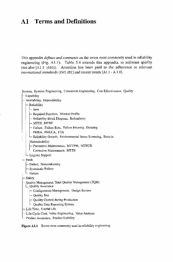
This appendix defines und comments on the terms most commonly used in reliability engineering (Fig. Al.1). Table 5.4 extends this appendix to Software quality (See also [ A I S (610)l. Attention has been paid to the adherence to relevant international standards (ISO, IEC) and recent trends [Al .1 - A. 1.81.
System, Systems Engineering, Concurrent Engineering, Cost Effectiveness, Quality - Capability - Availability, Dependability - Reliability
1 Item Required Function, Mission Profile Reliability Block Diagram, Redundancy
MTTF, MTBF Failure, Failure Rate, Failure Intensity, Derating
FMEA, FMECA, FTA Reliability Growth, Environmental Stress Screening, Bum-in
Maintainability
t Preventive Maintenance, MTTPM, MTBUR
Corrective Maintenance, MTTR
- Logistic Support
- Fault
F Defect, Nonconformity Systematic Failure
Failure - Safety - Quality Management, Total Quality Management (TQM) L Quality Assurance
t Configuration Management, Design Review
Quality Test Quality Control during Production
Quality Data Reporting System
- Life Time, Useful Life - Life-Cycle Cost, Value Engineering, Value Analysis - Product Assurance, Product Liability
Figure A l . l Terms most commonly used in reliability engineering
A l Terms and Definitions
Availability, Point Availability (A(t), PA(t))
Probability that the item is in a state to perform the required function at a given instant of time.
Instantaneous availability is often used. The use of A(t) shouId be avoided, to elude confusion with other kind of availability (e.g. average availability A A(t ), mission availability M A(TO, to), and work-mission availability WM A(TO, X ) in Section 6.2). A qualitative definition, focused on ability, is also possible. The term item stands for a structnral unit of arbitrary complexity. Computation generally assumes continuous operation (item down only for repair), renewal at failure (good-as-new after repair), and ideal human factors & logistic support. For an item with more than one element, good-as-new after repair refers in this book to the repaired element in the reliability block diagram. This assumption is valid for the whole item (system), only in the case of constant failure rates for all elernents. Assuming renewal for the whole item, the asymptotic &steady-state value of the point availability can be expressed by PA = MTTFI(MTTF+ MTTR). PA is also the asymptotic &
steady-state value of the average availability AA (often given as availability A).
Burn-in (nonrepairable items)
Type of screening test while the item is in operation.
For electronic devices, Stresses during burn-in are often constant higher ambient temperature (e.g. 125°C for ICs) and constant higher supply voltage. Burn-in can be considered as a part of a screening procedure, performed on a 100% basis to provoke early failures and to stabilize the characteristics of the item. Often it can be used as an accelerated reliability test to investigate the item's failure rate.
Burn-in (repairable items)
Process of increasing the reliability of hardware by employing functional operation of every items in a prescribed environment with corrective maintenance during the early failure period.
The term run-in is often used instead of burn-in. The stress conditions have to be chosen as near as possible to those expected infield operation. Flaws detected during burn-in can be detenninistic (defects or systematic failures) during the pilot production (reliability growth), but should be attributable only to early failures (randomly distributed) during the series production.
Capability
Ability to meet a service demand of given quantitative characteristics under given internal conditions.
Performance (technical performance) is often used instead of capability.
Al Terms and Definitions
Concurrent Engineering
Systematic approach to reduce the time to develop, manufacture, and market the item, essentially by integrating production activities into the design & development phase.
Concurrent engineering is achieved through intensive teamwork between all engineers involved in the design, production, and marketing of the item. It has a positive influence on the optimization of life-cycle cost.
Configuration Management
Procedure to specify, describe, audit, and release the configuration of the item, as well as to control it during modifications or changes.
Configuration includes all of the item's functional and physical characteristics as given in the documentation (to specify, build, test, accept, operate, maintain, and logistically support the item) and as present in the hardware andlor software. In practical applications, it is useful to subdivide configuration management into configuration identification, auditing, control (design reviews), and accounting. Configuration management is of particular importance during the design &
development phase.
Corrective Maintenance
Maintenance carried out after failure to restore the required function.
Corrective maintenance is also known as repair and can include any or all of the following steps: recognition, isolation (localization & diagnosis), elimination or removal (disassemble, remove, replace, reassemble), and function checkout. Repair is used in this book as a synonym for restoration. To simplify computation it is generally assumed that the repaired element in the reliability block diagram is as-good-as-new after each repair (also including a possible environmental stress Screening of the spare parts). This assumption applies to the whole item (equipment or system) if all elements of the item (which have not been renewed) have constant failure rates (seefailure rate for further comments).
Cost Effectiveness
Measure of the ability of the item to meet a service demand of stated quantitative characteristics, with the best possible usefulness to life-cycle cost ratio.
System effectiveness is often used instead of cost effectiveness.
Al Terms and Definitions
Defect
Nonfulfillment of a requirement related to an intended or specified use.
From a technical point of view, a defect is similar to a nonconfonnity, however not necessady from a legal point of view (in relation to product liability, nonconformity should be preferred). Defects do not need to influence the item's functionality. They are caused by flaws (errors, mistakes) dunng design, development, production, or installation. The term defect should be preferred to that of error, which is a cause. Unlike failures, which always appear in time (randomly distributed), defects are present at t = 0 . However, some defects can only be recognized when the item is operating and are referred to as dynamic defects (e.g. in software). Similar to defects, with regard to causes, are systematic failures (e.g. cooling problern); however, they are often not present at t=O.
DependabiIity
Collective term used to describe the availability performance and its influencing factors (reliability, maintainability, and logistic support).
Dependability is used generally in a qualitative sense, often defined as ability to provide the required function when demanded.
Derating
Designed reduction of stress from the rated value to enhance reliability.
The stress factor S expresses the ratio of actual to rated stress under normal operating conditions (generally at 25'C ambient temperature). Designed is used as a synonym for deliberate.
Design Review
Independent examination of the design to identify shortcomings that could affect the fitness for purpose, reliability, maintainability or maintenance support requirements of the item.
Design reviews are an important tool for quality assurance and T Q M during the design and development of hardware and software (Tables A3.3,5.3,5.5,2.8,4.3, Appendix A4). An important objective of design reviews is to decide about continuation or stopping the project considered on the basis of objective considerations and feasibility check (Tables A3.3 and 5.3, Fig. 1.6).
Environmental Stress Screening (ESS)
Test or set of tests intended to remove defective items, or those likely to exhibit early failures.
ESS is a screening procedure often perfonned at assembly (PCB) or equipment level on a 100% basis to find defects and systematic failures during the pilot production (reliability growth), or to provoke early failures in a series production. For electronic items, it consists generally of temperature cycles
A l Terms and Definitions 355
andlor random vibrations. Stresses are in general higher than in field operation, but not so high as to stimulate new failure mechanisms. Experience shows that to be cost effective, ESS has to be tailored to the item and production processes. At component level, the term screening is often used.
Failure
Termination of the ability to perform the required function.
Failures should be considered (classified) with respect to the mode, cause, effect, and mechanism. The cause of a failure can be intrinsic (early failure, failure with constant failure rate, wearont) or extrinsic (systematic failures, i. e. failures resulting from errors or mistakes in design, production, or operation which are deterministic and has to be considered as defects). The effect (consequence) of a failure is often different if considered on the directly affected item or on a higher level. A failure is an event appearing in time (randomly distributed), in contrast to a fault which is a state.
Failure Intensity ( z( t))
Limit, if it exists, of the mean number of failures of a repairable item within time interval ( t, t + St] , to 6 t when 6 t -+ 0.
At System level, zs ( t ) is used. Failure intensity applies for repairable items, in particular when repair times are neglected and failure occurrence is considered on the time axis (arrival times). It has been investigated for Poisson processes (homogeneous (z(t)= h) & nonhomogeneous (z(t)= m(t ))) and renewal processes (z(t)= h(t)) (Appendices A7.2, A7.8). For practical applications it holds that z(t)6t =Pr{v(t +6t)-v(t)=l), V ( t )= number of failures in (O,t] (Eq. (A7.229)). Seealso failure rate.
Failure Modes and Effects Analysis (FMEA)
Qualitative method of analysis that involves the study of possible failure modes and faults in subitems, and their effects on the ability of the item to provide the required function.
See FMECA for comments.
Failure Modes, Effects, and Criticality Analysis (FMECA)
Quantitative or qualitative method of analysis that involves failure modes und effects analysis together with a consideration of the probability of the failure mode occurrence and the severity of the effects.
Goal of a FMEA or FMECA is to identify all potential hazards and to analyze the possibilities of reducing their effect andlor occurrence probability. All possible failure modes and faults with the conesponding causes have to be considered bottom-up from lowest to highest integration level of the item considered. Often one distinguishes between design and production (process) FMEA or FMECA. FMECA can be used for fault modes, effects, and criticality analysis (same for FMEA).
Al Terms and Definitions
Failure Rate (q t ) )
Limit, if it exists, of the conditional probability that the failure occurs within time interval ( t , t + 6 t ] , to 6 t when 6 t + 0, given that the item was new at t = 0 and did not fail in the interval (0, t ] .
At system level, h s ( t ) is used. The failure rate applies in particular for nonrepairable items. In this case, i f z is the item failure-free time, with distribution function F(t) = Pr(t I t } , with F(O)= 0 and density f(t ), the failure rate h ( t ) follows as (Eq. (A6.25), R(t ) = 1 - F(t ))
1 f(t) dR( t ) ld t h ( t ) = lim - R ( t < t ~ t + 8 t l ~ > t } = - = - - - - .
6t10 6t 1 - F(t) W )
Considering R(0) = I , Eq. ( A l . l ) yields R( t ) = e-1; h (x )m and thus, R( t ) = echt for h( t ) = h . This important result characterizes the memoryless property o f the exponential distribution F(t)=l- e -h f , expressed by Eq. ( A l . l ) for h ( t ) = h . Only for h ( t ) = h one can estimate the failure rate h by h = k l 7: where T is the given (fixed) cumulative operating time and k> 0 the total number o f failures during T (Eq. (7.28)). Figure 1.2 shows a typical shape of h ( t ) . However,consid- ering Eq. (A l . l ) , the failure rate can be defined also for repairable items which are as-good-as-new after repair (restoration), taking instead of t the variable x starting by x = 0 at each repair (as for interarrival times). This is important when investigating repairable Systems (Chapter 6), e.g. with constant failure & repair rates. I f a repairable system cannot be restored to be as-good-as-new after repair (with respect to the state considered), i.e i f at least one element with time dependent failure rate has not been renewed at every repair, failure intensiv z ( t ) has to be used. It is thus important to distinguish between failure rate h ( t ) and failure intensiv z ( t ) or intensity ( h ( t ) or m ( t ) for a renewal or Poisson process). z ( t ) , h ( t ) , m ( t ) are unconditional densities (Eqs. (A7.229), (A7.24), (A7.194)) and differ basically from h( t ) which is a conditional density. This distinction is important also for the case o f a homogeneous Poisson process, for which z(t)=h (t)= m(t)=h holds for the intensity and h ( x ) = h holds for the interarrival times ( X starting by 0 at each interarrival time,Eq. (A7.38)). To reduce ambiguities, force of mortality has been suggested for h ( t ) [6.3, A7.301.
Fault
State characterized by an inability to perform the required function due to an internal reason.
A fault is a state and can be a defect or a failure, having thus as possible cause an error (for defects or systematic failures) or a failure mechanism (for failures).
Fault Tree Analysis @TA)
Analysis utilizing fault trees to determine which faults of subitems, or external events, or combination thereof, may result in item faults.
FTA is a top-down approach, which allows the inclusion o f extemal causes more easily than a FMEAl FMECA. However, it does not necessarily go through all possible fault modes. Combination o f FMEA I FMECA with FTA leads to causes-to-effects chart, showing the logical relationship between identified causes and their single or multiple consequences. A graphical descrip- tion of cause-to-effect relationships is the cause-to-effect diagram fishbone or Ishikawa diagram).
A l Terms and Definitions
Item
Part, component, device, functional unit, subsystem or system that can be individually described and considered.
An item is a functional or structural unit, generally considered as an entitj for investigations. It can consist of hardware andlor software and include human resources.
Life Cycle Cost (LCC)
Sum of the cost for acquisition, operation, maintenance, and disposal or recycling of the item.
Life-cycle cost have to consider also the effects to the environment of the production, use, and dispos- al or recycling of the item considered (sustainable development). Their optimization uses cost effec- tiveness or Systems engineering tools and can be positively influenced by concurrent engineering.
Lifetime
Time span between initial operation and failure of a nonrepairable item.
Logistic Support
All activities undertaken to provide effective and economical use of the item during its operating phase.
An emerging aspect related to logistic support is that of obsolescence management, i.e. how to assure operation over e.g. 20 years when components need for maintenance are no longer manufactured.
Maintainability
Probability that a given maintenance action, performed under stated conditions and using stated procedures and resources, can be carried out within a stated time interval.
Maintainability is a characteristic of the item and refers to preventive and corrective maintenance. A qualitative definition, focused on ability, is also possible. In specifying or evaluating maintainabi- lity, it is important to consider the logistic support available (procedures, personnel, spare Parts, etc.).
Mission Profile
Specific task which must be fulfilled by the item during a stated time under given conditions.
The mission profile defines the required function and the environmental conditions as a function of time. A system with a variable required function is termed a phased-mission system.
Al Terms and Definitions
MTBF
Mean operating time between failures.
At system level, MTBFs is used. MTBF applies for repairable items. However, for practical applications it is important to recognize that successive operating times between system failures have the Same mean (expected value) only if they are independent and have a common distribution function, i.e. if the system is as-good-as-new after each repair at system level. If only the failed element is restored to as-good-as-new after repair and at least one nonrestored element has a time dependent failure rate, successive operating times between system failures are neither independent nor have a common distribution. Only the case of a series-system with constant failure rates hl,...,h, for all elements EI, ..., E, yields to a homogeneous Poisson process, for which successive interarrival times (operating times between system failures) are inde endent and exponentially
- distributed with common distribution function ~ ( x ) = ~ - e - ~ ( ' ~ ' . ' *R1z ) - 1-e-I 'S and mean MTBF' = 1 Ihs (repaired elements are assumed as-good-as-new, yielding system as-good-as-new because of the constant failure rates hl,...,h,). This result holds approximately also for systems with redundancy (see Eq. (6.93) and comments with M77'F). For all these reasons, and also because of the estimate MTBF= T I L, often used in practical applications, MTBF should be confined to repai- rable systems with constanr failure rates for all elements. Shortcomings because of neglecting this basic property are known, see e.g. [6.3,7.1 l,A7.30]. As in the previous editions of this book, MTBFs will be reserved for the case
For Markov and semi-Markov models, MUTs is used.
MTTF
Mean time to failure.
At system level, MTTFs is used. MTTF is the mean (expected valueJ of the item failure-free time T. It can be computed from the reliability function R(t) as MTTF = R(t ) d t , with TL as the upper limit of the integral if lhe: life time is limited to TL (R(t)= 0 for t > TL ). MTTF applies for both nonrepairable and repairable items if one assumes that after repair the item is as-good-as-new (p. 40). At system level, this occurs (with respect to the state considered) only if the repaired element is as-good-as-new and all nonrepaired elements have constant failure rates. To inclnde for this case all situations, M7TFsi is used in Chapter 6 (S stands for system and i for the state occupied (entered for a semi-Markov process) at the time at which the repair (restoration) is terminated, see e.g. Table 6.2). When dealing with failure-free and repair times, the variable x starting by X = 0 after each repair (restoration) has to be used instead of t (as for interarri~al~times). See p. 40 for further comments. An unbiased, empirical estimate for MTTF is M77F = (tl + ... + t,)l n , where t l , . . . , tn are observed failure-free times of n statistically identical and independent items.
MTTPM
Mean time to preventive maintenance.
See MTTR for comments.
Al Terms and Definitions
MTBUR
Mean time between unscheduled removals.
MTTR
Mean time to repair.
At system level, M7TRS is used. Repair is used in this book as a synonym for restoration. MTTR is the mean (expected value) of the item mpair time. It can be computed from the distnbution function G(t) of the repair time as MZTR = I. (1 - G(t ))dt . In spsifying or evaluatiiig M7TR. it is neces- sary to consider the logistic support available for repair (procedures, personnel, spare Parts, test facilities). Repair time is often lognormally distributed. However, for reliability or availability computation of repairable equipment and Systems, a constant repair rate p (i.e. exponentially distributed repair times with = 1 I MTTR) can be used in general to get valid approximate results, as long as MTTR << M l T F holds for each element in the reliability block diagram (Examples 6.7, 6.8, 6.9). An unbiased, empincal estimate of MTTR is M ~ T R = (tl + . . . + t,) l n, where tl, . . ., t, are observed repair times of n statistically identical and independent items.
Nonconformity
Nonfulfillment of a specified requirement.
From a technical point of view, nonconformity is close to defect, however not necessarily from a legal point of view. In relation to product liability, nonconformity should be preferred.
Preventive Maintenance
Maintenance carried out to reduce the probability of failure or degradation.
The aim of preventive maintenance must also be to detect and remove hidden failures, i.e. non- recognized failures in redundant elements. To simplify computation it is generally assumed that the element in the reliability block diagram for which a preventive maintenance has been performed is as-good-as-new after each preventive maintenance. This assumption applies to the whole item (equipment or system) if all components of the item (which have not been renewed) have constant failure rates. Preventive maintenance is generally performed at scheduled time intervals.
Product Assurance
All planned and systematic activities necessary to reach specified targets for the reliability, maintainability, availability, and safety of the item, as well as to provide adequate confidence that the item will meet all given requirements.
The concept of product assurance is used in particular in aerospace programs. It includes quality assurance as well as reliability, maintainability, availability, safety, and logistic suppori engineering.

Al Terms and Definitions
Product Liability
Generic term used to describe the onus on a producer or others to make restitution for loss related to personal injury, property damage, or other harm caused by the product.
The manufacturer (producer) has to speczfj> a safe operational mode for the product (item). If strict liability applies, the manufacturer has to demonstrate (at a claim) that the product was free from defects when it left the production plant. This holds in the USA and partially also in Europe [1.8]. However, in Europe the causality between damage and defect has still tobe demonstrated by the User and the limitation period is short (often 3 years after the identification of the damage, defect, and manufacturer, or 10 years after the appearance of the product on the market). One can expect that liability will more than before consider faults (defects & failures) and Cover software as well. Product liability forces producers to place greater emphasis on quality assurance Imanagement.
Quality
Degree to which a Set of inherent characteristics fulfills requirements.
This definition, given also in the ISO 9000:2000 Standard [A1.6, A2.91, follows closely the traditional definition of quality fitness for use) and applies to products and semices as well.
Quality Assurance
All the planned and systematic activities needed to provide adequate confidence that quality requirements will be fulfilled.
Quality assurance is a part of quality management, as per ISO 9000: 2000. It refers to hardware and software as well, and includes configuration management, quality tests, quality control during production, quality data reporting systems, and software quality (Fig. 1.3). For complex equipment and systems, quality assurance activities are coordinated by a quality assurance program (Appendix A3). An important target for quality assurance is to achieve the quality requirements with a minimum of cost and time. Concurrent engineering also strive to short the time to develop and market the product.
Quality Control During Production
Control of the production processes and procedures to reach a stated quality of manufacturing.
Quality Data Reporting System
System to collect, analyze, and correct all defects and failures occurring during production and testing of the item, as well as to evaluate and feedback the corresponding quality and reliability data.
Al Terms and Definitions 361
A quality data reporting system is generally Computer aided. Analysis of defects and failures must be traced to the cause in order to determine the best corrective action necessary to avoid repetition of the same problem. The quality data reporting system should also remain active during the operating phase. A quality data reporting system is important to monitor reliability growth.
Quality Management
Coordinated activities to direct and control an organization with regard to quality.
Organization is defined as group of people und facilities (e.g. a company) with an arrangement of responsibilities, authorities, und relationships [A1.6].
Quality Test
Test to verify whether the item conforms to specified requirements.
Quality tests include incoming inspections, qualification tests, production tests, and acceptance tests. They also Cover reliability, maintainability, and safety aspects. To be cost effective, quality tests must be coordinated and integrated in a test (und screening) strategy. The terms test and inspection are often used for quality test.
Redundancy
Existence of more than one means for performing the required function.
For hardware, distinction is made between active (hot, parallel), warn (lightly loaded), and standby (cold) redundancy. Redundancy does not necessarily imply a duplication of hardware, it can for instance be implemented at the software level or as a time redundancy. To avoid common mode failures, redundant elements should be realized independently from each other. Should the redundant elements fulfill only a part of the required function, a pseudo redundancy is present.
Reliability ( R , R( t ) )
Probability that the required function will be provided under given conditions for a given time interval.
According to the above definition, reliability is a characteristic of the item, generally designated by R for the case of a fixed mission and R(t ) for a mission with t as a Parameter. At system level RSi ( t ) is used, where S stands for system and i for the state entered at t = 0 (Table 6.2). A qualitative definition, focused on abili@, is also possible. Reliability gives the probability that no operational interruption at item (system) level will occur during a stated mission, say of duration T. This does not mean that redundant parts may not fail, such parts can fail and be repaired. Thus, the concept of reliability applies for nonrepairable as well as for repairable items. Should T be considered as a variable t , the reliabilityfunction is given by R(t) . If z is the failure-free time, distributed according to F(t) , with F(0) = 0, then R(t ) = Pr(7 > t ) = 1 - F(t ) . . The concept of reliability can also be used for processes or sewices, although modeling human aspects can lead to some difficulties.
A l Terms and Definitions
Reliability Block Diagram
Block diagram showing how failures of subitems, represented by the blocks, can result in a failure of the item.
The reliability block diagram (RBD)is an event diagram. It answers the question: Which elements of the item are necessary to fulfill the required function und which ones can fail without affecting it? The elements (blocks in the RBD) which mnst operate are connected in series (the ordering of these elements is not relevant for reliability computation) and the elements which can fail (redundant elements) are connected in parallel. Elements which are not relevant (used) for the required function are removed from the RBD and put into a reference list, after having verified (PMEA) that their failure does not affect elements involved in the required function. In a reliability block diagram, redundant elements still appear in parallel, irrespective of the failure mode. However, only one failure mode (e.g. short, open) and two states (good , failed) can be considered for each element.
Reliability Growth
Progressive improvement of a reliability measure with time.
Flaws (errors, mistakes) detected during a reliability growth program are in general deterministic (defects or systematic failures) and present in every item of a given lot. Reliability growth is thus often performed during the pilot production, seldom for series-produced items. Similarly to environmental stress screening (ESS), Stresses during reliability growth often exceed those expected in field operation, but not so high as to stimulate new failure mechanisms. Models for reliability growth can also often be used to investigate the occurrence of defects in sofnvare. Even if software defects often appear in time (dynamic defects), tbe term sofrware reliability should be avoided (sofnvare quality should be preferred).
Required Function
Function or combination of functions of an item which is considered necessary to provide a given service.
The definition of the required function is the starting point for every reliability analysis, as it defines failures. However, difficulties can appear with complex items (systems). For practical purposes, Parameters should be specified with tolerances.
Safety
Ability of the item to cause neither injury to persons, nor significant material damage or other unacceptable consequences.
Safety expresses freedom from unacceptable risk of harm. In practical applications, it is useful to subdivide safety into accidentprevention (the item is safe working while it is operating correctly) and technical safety (the item has to remain safe even if a failure occurs). Technical safety can be defined
A l Terms and Definitions 363
as the probability that the item will not cause i n j u ~ topersons, signzjicant material damage or other unacceptable consequences above a given (fked) level for a stated time interval, when operating under given conditions. Methods and procedures used to investigate technical safety are similar to those used for reliability analyses, however with emphasis on fault lfailure effects.
System
Set of interrelated items considered as a whole for a defined purpose.
A system generally includes hardware, software, semices, and personnel (for operation and support) to the degree that it can be considered self-sufficient in its intended operational environment. For computations, ideal conditions for human factors and logistic support are often assumed, leading to a technical system (for simplicity, the term system is often used instead of technical system). Elements of a system are e.g. components, assemblies, equipment, and subsystems, for hardware. For maintenance purposes, systems are partitioned into independent line replaceable units (LRUs), i.e. spare parts at equipment or system level. The term item is used for a functional or structural unit of arbitrary complexity that is in general considered as an entity for investigations.
Systematic Failure
Failure related in a deterministic way to a certain cause inherent in the design, manufacturing, operation or maintenance processes.
Systematic failures are also known as dynamic defects, for instance in software quality, and have a deterministic character. However, because of the item complexity they can appear as if they were randomly distributed in time.
Systems Engineering
Application of the mathematical and physical sciences to develop systems that utilize resources economically for the benefit of society.
TQM and concurrent engineering can help to optimize systems engineering.
Total Quality Management (TQM)
Management approach of an organization centered on quality, based on the participation of all its members, and aiming at long-term success through customer satisfaction, and benefits to all members of the organization and to socieiy.
Within TQM, everyone involved in the product (directly during development, production, installation, and semicing, or indirectly with management or staff activity) is jointly responsible for the quality of that product.
A l Tenns and Definitions
Useful Life
Time interval starting when the item is first put into operation and ending when a limiting state is reached.
The limiting state can be an unacceptable failure intensity or other. Typical values for useful life are 3 to 6 years for commercial applications, 5 to 15 years for military installations, and 10 to 30 years for distribution or power Systems (see also Lifetime).
Value Analysis
Optimization of the configuration of the item as well as of the production processes and procedures to provide the required item characteristics at the lowest possible cost without loss of capability, reliability, maintainability, or safety.
Value Engineering
Application of value analysis methods during the design phase to optimize the life-cycle cost of the item.

A2 Quality and Reliability Standards
Besides quantitative reliability requirements, such as MTBF = 1 l ?L, MTTR, and availability, customers often require a quality assurance /management System and for complex items also the realization of a quality und reliability assurance program. Such general requirements are covered by national and international standards, the most important of which are briefly discussed in this appendix. The term management is used explicitly where the organization (company) is involved as a whole, as per ISO 9000: 2000 and TQM. A basic procedure for setting up and realizing quality and reliability requirements for complex equipment and systems, with the corresponding quality und reliability assurance program, is discussed in Appendix A3.
A2.1 Introduction
Customer requirements for quality and reliability can be quantitative or qualitative. As with performance Parameters, quantitative reliability requirements are given in system specifications or contracts. They fix targets for reliability, maintainability, availability, and safety (as necessary) along with associated specifications for required function, operating conditions, logistic support, and criteria for acceptance tests. Qualitative requirements are in national or international standards and generally deal with a quality management system. Depending upon the field of application (aerospace, defense, nuclear, or industrial), these requirements may be more or less stringent. Objectives of such standards are in particular:
1. Harmonization of quality management systems and of terms & definitions.
2. Enhancement of customer satisfaction.
3. Standardization of configuration, operating conditions, logistic support, test procedures, and selectionl qualification criteria for components, materials, and production processes.
Important standards for quality management systems are given in Table A2.1, see [A2.1 - A2.131 for a comprehensive list. Some of the standards in Table A2.1 are briefly discussed in the following sections.

366 A2 Quality and Reliability Standards
A2.2 General Requirements in the Industrial Field
In the industrial field, the ISO 9000: 2000 family of standards [A2.9] supersedes the ISO 9000: 1994 family and Open a new era in quality management requirements. The previous 9001 - 9004 are substituted by 9001: 2000 and 9004: 2000. The ISO 8402, on definition, is substituted by the ISO 9000: 2000. Many definitions have been revised and the structure and content of 9001: 2000 and 9004: 2000 are new, and adhere better to the industrial needs and to the concept depicted in Fig. 1.3. Eight basic quaIity management principles have been identified and considered in the ISO 9000: 2000 family: Customer Focus, Leadership, Involvement of People, Process Approach, System Approach to Management, Continuous Improvement, Factual Approach to Decision Making, and Mutually Beneficial Supplier Relationships.
ISO 9000:2000 describes fundamentals of quality management Systems and specify the terminology involved.
ISO 9001: 2000 specifies requirements for a quality management system that an organization (company) needs to demonstrate its ability to provide products that satisfying customer und applicable regulatory requirements. It focus on four main chapters: Management Responsibility, Resource Management, Product and / or Service Realization, and Measurement. A quality management system must ensure that everyone involved with a product (whether in its development, production, installation, or servicing, as well as in a management or staff function) shares responsibility for the quality of that product, in accordance to TQM. At the same time, the system must be cost effective and contribute to a reduction of the time to market. Thus, bureaucracy must be avoided and such a system must Cover all aspects related to quality, reliability, maintainability, availability, and safety, including management, organization, planning, and engineering activities. Customer expects today that only items with agreed requirements will be delivered.
ISO 9004: 2000 provides guidelines that consider efficiency und effectiveness of the quality management system.
The ISO 9000: 2000 family deals with a broad class of products and services (technical and non-technical), its content is thus lacking in details, compared with application specific standards used e.g. in railway, aerospace, defense , and nuclear industries (Appendix A2.3). It has been accepted as national standards in many countries, and international recognition of certification has been partly achieved.
Dependability aspects, focusing on reliability, maintainability, and logistic support of systems are considered in IEC Standards, in particular IEC 60300 for global requirements and IEC 60605, 60706, 60812, 60863, 61025, 61078, 61124, 61163, 61164, 61165, 61508, und 61709for specific procedures, see [A2.6] for a comprehensive list. IEC 60300 deals with dependability programs (management, task descriptions, application guides). Reliability tests for constant failure rate ?L
(or of MTBF for the case MTBF = 1 l h ) are considered in IEC 61 124. Maintainability aspects are in IEC 60706 and s a f e ~ , aspects in IEC 61508.
A2.2 General Requirements in the Industrial Field 367
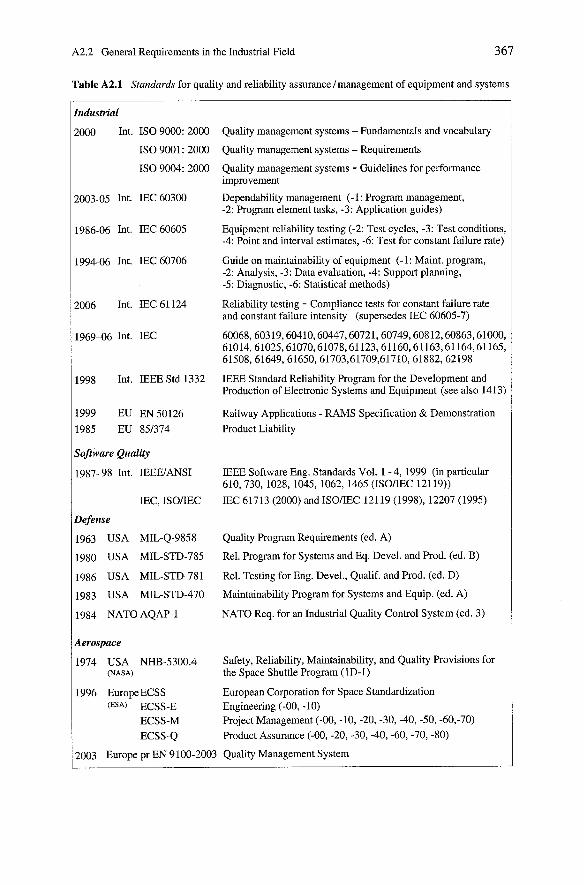
Table A2.1 Standards for quality and reliability assurance lmanagement of equipment and systems
'ndustriul
~ 0 0 0 Int. ISO 9000: 2000
ISO 9001 : 2000
ISO 9004: 2000
1986-06 Int. IEC 60605
1994-06 Int. IEC 60706
l006 Int. IEC 61124
1998 Int. IEEE Std 1332
goftware Quality
1987- 98 Int. IEEEIANSI
IEC, ISOAEC
9efense
1963 USA MIL-Q-9858
1980 USA MIL-STD-785
L986 USA MIL-STD-781
1983 USA MIL-STD-470
1984 NATO AQAP-1
Qerospace
1974 USA NHB-5300.4 (NASA)
1996 EuropeECSS (EsAl ECSS-E
ECSS-M ECSS-Q
Quality management systems - Fundamentals and vocabulary
Quality management systems - Requirements
Quality management systems - Guidelines for performance improvement
Dependability management (-1: Program management, -2: Program element tasks, -3: Application guides)
Equipment reliability testing (-2: Test cycles, -3: Test conditions -4: Point and interval estimates, -6: Test for constant failure rate)
Guide on maintainability of equipment (-1: Maint. program, -2: Analysis, -3: Data evaluation, -4: Support planning, -5: Diagnostic, -6: Statistical methods)
Reliability testing - Compliance tests for constant failure rate and constant failure intensity (supersedes IEC 60605-7)
60068,60319,60410,60447,60721,60749,60812,60863,61000 61014,61025,61070,61078,61123,61160,61163,61164,61165 61508,61649,61650,61703,61709,61710,61882,62198
IEEE Standard Reliability Program for the Development and Production of Electronic Systems and Equipment (see also 1413
Railway Applications - RAMS Specification & Demonstration Product Liability
IEEE Software Eng. Standards Vol. 1 - 4, 1999 (in particular 610,730, 1028, 1045, 1062, 1465 (ISOIIEC 12119))
IEC 61713 (2000) and ISOnEC 12119 (1998), 12207 (1995)
Quality Program Requirements (ed. A)
Rel. Program for Systems and Eq. Devel. and Prod. (ed. B)
Rel. Testing for Eng. Devel., Qualif. and Prod. (ed. D)
Maintainability Program for Systems and Equip. (ed. A)
NATO Req. for an Industrial Quality Control System (ed. 3)
Safety, Reliability, Maintainability, and Quality Provisions for the Space Shuttle Program (1D-1)
European Corporation for Space Standardization Engineering (-00, - 10) Project Management (-00, -10, -20, -30, -40, -50, -60,-70) Product Assurance (-00, -20, -30, -40, -60, -70, -80)
2003 Europe pr EN 9 100-2003 Quality Management System
368 A2 Quality and Reliability Standards
For electronic equipment & Systems, IEEE Std 1332-1998 [A2.7] has been issued as a guide to a reliability program for the development and production phases. This document gives in a short form the basic requirements, putting an accent on an active cooperation between supplier (manufacturer) and customer, and focusing three main aspects: Determination of the Customer's Requirements, Determination of a Process that satisfy the Customer's Requirements, and Assurance that the Customer's Requirements are met. Examples of comprehensive requirements for industry application are e.g. in [A2.2, A2.31. Software aspects are considered in IEEE Software Engineering Standards [A2.8]. Requirements for product liability are given in national and international directives, see for instance [1.8].
A2.3 Requirernents in the Aerospace, Railway, Defense, and Nuclear Fields
Requirements in space und railwayfields generally combine the aspects of quality, reliability, maintainability, safety, and software quality in a Product Assurance or RAMS document, well conceived in its structure& content [A2.3 - A2.5, A2.121. In the railway field, EN 50126 [A2.3] requires a RAMS program with particular emphasis on safety aspects. Similar is in the avionics field, where EN 9100-2003 [A2.4] has been issued by reinforcing requirements of ISO 9000 family. It can be expected that space and avionics will unify standards in an Aerospace Series.
MIL-Standards have played an important role in the last 30 years, in particular MIL-Q-9858 and MIL-STD-470, -471, -781, 785 & -882 [A2.10]. MIL-Q-9858 (first Ed. 1959) was the basis for many quality assurance standards. However, as it does not Cover specific aspects of reliability, maintainability, and safety, MIL-STD-785, -470, and -882 were issued. MIL-STD-785 requires the realization of a reliability program; tasks are carefully described and the program has to be tailored to satisfy User needs. MTBF = 11 h acceptance procedures are in MIL-STD-781. MIL-STD-470 requires the realization of a maintainability program, with emphasis on design d e s , design reviews, and FMEAI FMECA. Maintainability demonstration is covered by MIL- STD-471. MZL-STD-882 requires the realization of a safety program, in particular the analysis of all potential hazards. For NATO countries, AQAP Requirements were issued starting 1968. MIL Standards have dropped their importance. However, they can still be useful in developing procedures for industrial applications.
The nuclearfield has its own specific, well established standards with emphasis on safety aspects, design reviews, configuration accounting, qualification of components / materials/production processes, quality control during production, and tests.
A3 Definition and Realization of Quality and Reliability Requirements
In defining quality und reliability requirements, it is important that market needs, life cycle cost aspects, time to market as well as development and production risks (for instance when using new technologies) are consider with care. For complex equipment und Systems with high quality & reliability requirements, the realization of such requirements is best achieved with a quality und reliability assurance program, integrated in the project activities andperformed without bureaucracy. Such a program (plan if time schedule is considered) defines the project specific activities for quality and reliability assurance and assigns responsibilities for their realization in agreement to TQM. This appendix discusses first important aspects in defining quality & reliability requirements and then the content of a quality and reliability assurance program for complex equipment und Systems with high qualiq und reliabiliiy requirements for the case in which tailoring is not mandatory. For less stringent requirements, tailoring is necessary to meet real needs and to be cost and time effective. Software specific quality assurance aspects are considered in Section 5.3. Examples for check lists for design reviews are in Appendix A4, requirements for a quality data reporting system in Appendix A5.
A3.1 Definition of Quality and Reliability Requirements
In defining quantitative, project specific, quality und reliability requirements attention has to be paid to the actual possibility to realize them as well as to demonstrate them at a final or acceptance test. These requirements are derived from customer or market needs, taking care of limitations given by technical, cost, and ecological aspects. This section deals with some important considerations by setting MTBF, M V R , and steady-state availability (PA = AA) requirements. MTBF is used for MTBF = 1 / A, where is the constant (time independent) failure rate of the item considered. Tentative targets for MTBF, MTl'R, PA are set by considering
operational requirements relating to reliability, maintainability, and availability, allowed logistic support,
370 A3 Definition and Realization of Quality and Reliability Requirements
required function and expected environmental conditions, experience with similar equipment or Systems,
possibility for redundancy at higher integration level,
requirements for life-cycle cost, dimensions, weight, power consumption, etc., ecological consequences (sustainability).
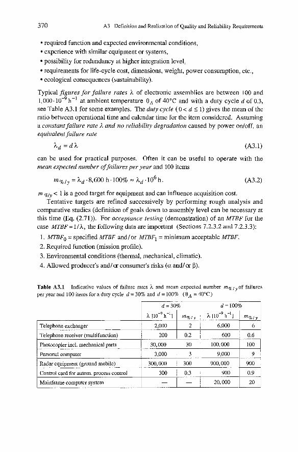
Typical Jigures for failure rates h of electronic assemblies are between 100 and l,OO0.10-~ h-l at ambient temperature B A of 40°C and with a duty cycle d of 0.3, See Table A3.1 for some examples. The duty cycle ( 0 < d I 1) gives the mean of the ratio between operational time and calendar time for the item considered. Assuming a constant failure rate A und no reliability degradation caused by power onloff, an equivalent failure rate
can be used for practical purposes. Often it can be useful to operate with the mean expected number of failuresper year and 100 items
rn < 1 is a good target for equipment and can influence acquisition cost. Tentative targets are refined successively by performing rough analysis and
comparative studies (definition of goals down to assembly level can be necessary at this time (Eq. (2.71)). For acceptance testing (demonstration) of an MTBF for the case MTBF = l l h , the following data are important (Sections 7.2.3.2 and 7.2.3.3):
1. MTBFo = specified MTBF andlor MTBFl = minimum acceptable MTBF.
2. Required function (mission profile).
3. Environmental conditions (thermal, mechanical, climatic).
4. Allowed producer's andlor consumer's risks (a andlor P).
Table A3.1 Indicative values of failure rates ?L and mean expected number msl of failures per year and 100 items for a duty cycle d = 30% and d = 100% ( B A = 40°C)
Telephone exchanger
Telephone receiver (multifunction)
Photocopier incl. mechanical parts
2,000
200
30,000
Personal computer 3,000 3
Radar equipment (ground mobile)
Control card for autom. process control
Mainframe computer system
2
0.2
30
300
0.3
-
300,000
300
-
6,000
600
100,000
900,000
900
20,000
6
0.6
100
900
0.9
20
A3.1 Definition of Quality and Reliability Requirements 371
5. Cumulative operating time T and number C of allowed failures during T (acceptance conditions).
6. Number of systems under test ( T / MTBFO as a rule of thumb).
7. Parameters which should be tested and frequency of measurement. 8. Failures which should be ignored for the MTBF acceptance test.
9. Maintenance and screening before the acceptance test.
10. Maintenance procedures during the acceptance test.
11. Form and content of test protocols and reports. 12. Actions in the case of a negative test result.
For acceptance testing (demonstration) of an MTTR, the following data are important (Section 7.3.2):
1. Quantitative requirements (MTTR, variante, quantile).
2. Test conditions (environment, personnel, tools, external Support, spare parts).
3. Number and extent of repairs to be undertaken (simulated/introduced failures).
4. Allocation of the repair time (diagnostic, repair, functional test, logistic time).
5. Acceptance conditions (number of repairs and observed empirical MTTR).
6. Form and content of test protocols and reports. 7. Actions in the case of a negative test result.
Availability usually follows from the relationship PA = MTBFI(MTBF + MTTR). However, specific test procedures for PA = AA are given in Scction 7.2.2).
A3.2 Realization of Quality and Reliability Require- ments for Complex Equipment and Systems
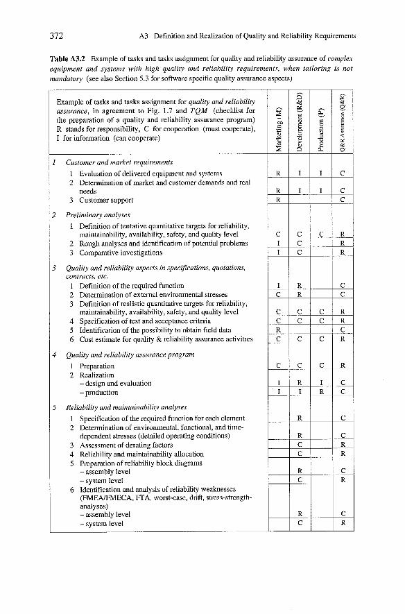
For complex items, in particular at equipment and system level, quality and relia- bility targets are best achieved with a quality und reliability assurance program, integrated in the project activities and performed without bureaucracy. In such a program, project specific tasks and activities are clearly described and assigned. Table A3.2 can be used as a checklist by defining the content of a quality and relia- bility assurance program for complex equipment und systems with high quality und reliability requirements, when tailoring is not mandatory (see also [A2.8 (730-2002)] and Section 5.3 for software specific quality assurance aspects). Table A3.2 is a refinement of Table 1.2 and shows a possible task assignment in a company as per Fig. 1.7. Depending on the item technology and complexity, or because of tailoring, Table A3.2 is to be shortened or extended. The given responsibilities for tasks (R, C, I) can be modified to reflect the company's personnel situation. For a comprehen- sive description of reliability assurance tasks see e.g. [A2.6 (60300), A2.10 (785), A3.11.
372 A3 Definition and Realization of Quality and Reliability Requirements
Table A3.2 Example of tasks and tasks assignment for quality and reliability assurance of complex equipment und systems with high quality und reliability requirements, when tailoring is not mandatory (see also Section 5.3 for software specific quality assurance aspects)
Example of tasks and tasks assignment for quality und reliability assurance, in agreement to Fig. 1.7 and TQM (checklist for the preparation of a quality and reliability assurance program) R stands for responsibility, C for cooperation (must cooperate), I for information (can cooperate)
Customer und rnarket requirements
1 Evaluation of delivered equipment and systems 2 Detennination of market and customer demands and real
needs 3 Customer Support
! Preliminary analyses
1 Definition of tentative quantitative targets for reliability, maintainability, availability, safety, and quality level
2 Rough analyses and identification of potential problems 3 Comparative investigations
Qualio und reliability aspects in specifications, quotations, contracts, etc.
1 Definition of the required function 2 Determination of extemal environmental stresses 3 Definition of realistic quantitative targets for reliability,
maintainability, availability, safety, and quality level 4 Specification of test and acceptance criteria 5 Identification of the possibility to obtain field data 6 Cost estimate for quality & reliability assurance activities
Quality und reliability assurance program
1 Preparation 2 Realization
- design and evaluation - production
i Reliability und maintainability analyses
1 Specification of the required function for each element 2 Determination of environmental, functional, and time-
dependent stresses (detailed operating conditions) 3 Assessment of derating factors 4 Reliability and maintainability allocation 5 Preparation of reliability block diagrams
- assembly level - system level
6 Identification and analysis of reliability weaknesses (FMEA/FMECA, R A , worst-case, dnft, stress-strength- analy ses) - assembly level - system level
A3.2 Realization of Quality and Reliability Requirements
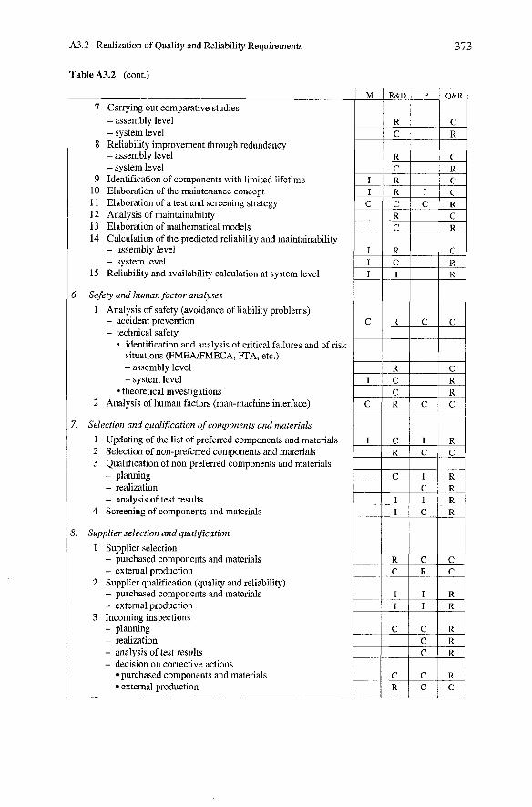
Table A3.2 (cont.)
7 Carrying out comparative studies - assembly level - system level
8 Reliability improvement through redundancy - assembly level - system level
9 Identification of components with limited lifetime 10 Elaboration of the maintenance concept I1 Elaboration of a test and screening strategy 12 Analysis of maintainability 13 Elaboration of mathematical models 14 Calculation of the predicted reliability and maintainability
- assembly level - system level
15 Reliability and availability calculation at system level
Safety und human factor analyses
1 Analysis of safety (avoidance of liability problems) - accident prevention - technical safetv
identification and analysis of critical failures situations (FMEAJFMECA, FTA, etc.) - assembly level
and of
-
risk
- system level theoretical investigations
2 Analysis of human factors (man-machine interface)
Selection und qualzjication of components und materials
1 Updating of the list of preferred components and materials 2 Selection of non-preferred components and materials 3 Qualification of non-preferred components aud materials
- planuing - realization - analysis of test results
4 Screening of components and materials
Supplier selection and qualification
1 Supplier selection - purchased components and materials - external production
2 Supplier qualification (quality and reliability) - purchased components and materials - extemal production
3 Incoming inspections - planning - realization - analysis of test results - decision on corrective actions
purchased components and materials extemal production
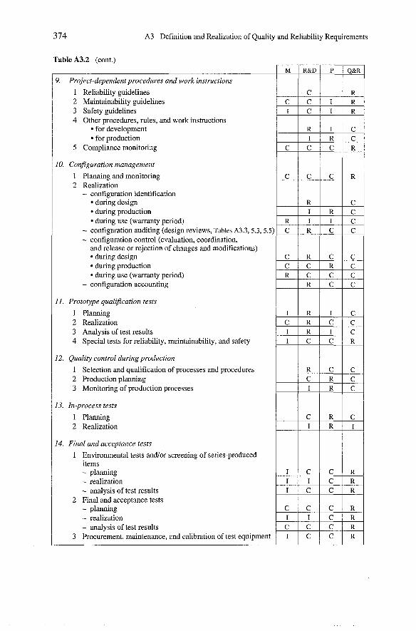
A3 Definition and Realization of Quality and Reliability Requirements 374
Table A3.2 (cont.)
10. Configuration manugement
1 Planning and monitoring 2 Realization
- configuration identification during design during production dunng use (warranty period)
- configuration auditing (design reviews, Tables A3.3,5.3,5.5) - configuration control (evaluation, coordination,
and release or rejection of changes and modifications) dunng design
3. Project-dependent procedures und work instructions
1 Reliability guidelines 2 Maintainability guidelines 3 Safety guidelines 4 Other procedures, rules, and work instructions
for development for production
5 Compliance monitoring
during production dunng use (warranty period)
- configuration accounting
11. Prototype qualification tests
1 Planning 2 Realization 3 Analysis of test results 4 Special tests for reliability, maintainability, and safety
M
12. Quality control during production
1 Selection and qualification of processes and procedures 2 Production planning 3 Monitoring of production processes
R&D
C
!3. Zn-process tests
1 Planning 2 Realization
14. Final und acceptance tests
P
C C I R I C I R
R I C I R C
C C C R
1 Environmental tests andlor screening of series-produced items - planning - realization - analysis of test results
2 Final and acceptance tests - plaming - realization - analvsis of test results
Q&R
R
C C C R C R
C C C R 3 Procurement, maintenance, and calibration of test equipment I C C R
A3.2 Realization of Quality and Reliability Requirements 375
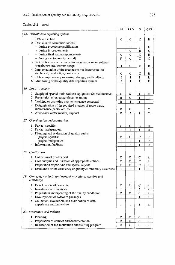
Table A3.2 (cont.)
/ 15. Quality data reporting system
1 Data collection 2 Decision on corrective actions
- during Prototype qualification - during in-process tests - during final and acceptance tests - during use (warranty penod)
3 Realization of corrective actions on hardware or software (repair, rework, waiver, scrap)
4 Implementation of the changes in the documentation (technical, production, customer)
5 Data compression, processing, Storage, and feedback 6 Monitoring of the quality data reporting system
1 16. Logistic suppori
1 Supply of special tools and test equipment for maintenance 2 Preparation of customer documentation 3 Training of operating and maintenance personnel 4 Determination of the required number of spare Parts,
maintenance personnel, etc. 5 After-sales (after market) support
17. Coordination and monitoring
3 Planning and realization of quality audits - project-specific - project-independent
4 Information feedback
18. Quality cost
1 Collection of quality cost 2 Cost analysis and initiation of appropnate actions 3 Preparation of periodic and special reports 4 Evaluation of the efficiency of quality & reliability assurance R
19. Concepts, methods, and general procedures (quality und reliability)
I Development of concepts 2 Investigation of methods 3 Preparation and updating of the quality handbook 4 Development of software packages R 5 Collection, evaluation, and distribution of data,
experience and know-how I I
20. Motivation und training 1 / 1 1 I Planning 2 Preparation of Courses and documentation 3 Realization of the motivation and training program R

376 A3 Definition and Realization of Quality and Reliability Requirements
A3.3 Elements of a Quality and Reliability Assurance Program
The basic elements of a quality and reliability assurance program, as defined in Appendix A.3.2, can be summarized as follows:
1. Project organization, planning, and scheduling
2. Quality and reliability requirements 3. Reliability and safety analysis
4. Selection and qualification of components, materials, and processes
5. Configuration management
6. Quality tests
7. Quality data reporting system
These elements are discussed in this section for the case of complex equipment and Systems with high quality and reliability requirements, when tailoring is not mandatory. In addition, Appendix A4 gives a catalog of questions to generate checklists for design reviews and Appendix A5 specifies the requirements for a quality data reporting System. For software specific quality assurance aspects one can refer to Section 5.3. As suggested in task 4 of Table A3.2, the realization of a quality and reliability assurance program should be the responsibility of the project manager. It is often useful to start with a quality and reliability program for the development phase, covering items 1 to 5 of the above list, and continue with the production phase for points 5 to 7.
A3.3.1 Project Organization, Planning, and Scheduling
A clearly defined project organization and planning is necessary for the realization of a quality and reliability assurance program. Organization and planning must also satisfy modern needs for cost management and concurrent engineering.
The system specification is the basic document for all considerations at project level. The following is a typical outline for system specifications:
1. State of the art, need for a new product
2. Target to be achieved
3. Cost, time schedule
4. Market potential (turnover, price, competition)
5. Technical performance
6. Environmental conditions
7. Operational capabilities (reliability, maintainability, availability, logistic support) 8. Quality and reliability

A3.3 Elements of a Quality and Reliability Assurance Program
9. Special aspects (new technologies, Patents, value engineering, etc.)
10. Appendices
The organization of a project begins with the definition of the main task groups. The following groups are usual for a complex system: Project Management, System Engineering, Life-Cycle Cost, Quality and Reliability Assurance, Assembly Design, Prototype Qualification Tests, Production, Assembly and Final Testing. Project organization, task lists, task assignment, and rnilestones can be derived from the task groups, allowing the quantification of the personnel, material, and financial resources needed for the project. The quality and reliability assurance program must require that the project is clearly and suitably organized and planned.
A3.3.2 Quality and Reliability Requirements
The most important steps in defining quality and reliability targets for complex equipment and Systems have been discussed in Appendix A.3.1.
A3.3.3 Reliability and Safety Analysis
Reliability and safety analyses include failure rate analysis, failure mode analysis (FMEAIFMECA, FTA), sneak circuit analysis (to identify latent paths which can cause unwanted functions or inhibit desired functions, while all components are functioning properly), evaluation of concrete possibilities to improve reliability and safety (derating, screening, redundancy), as well as comparative studies; see Chapters 2 - 6 for methods and tools.
The quality and reliability assurance program must show what is actually being done for the project considered. For instance, it should be able to supply answers to the following questions:
1. Which derating rules are considered?
2. How are the actual component-level operating conditions determined?
3. Which failure rate data are used? Which are the associated factors (TC, & xQ)?
4. Which tool is used for failure mode analysis? To which items does it apply? 5. Which kind of comparative studies will be performed?
6. Which design guidelines for reliability, maintainability, safety, and software quality are used? How will their adherence be verified?
Additionally, interfaces to the selection and qualification of components and materials, design reviews, test and screening strategies, reliability tests, quality data reporting system, and subcontractor activities must be shown. The data used for component failure rate calculation should be critically evaluated (source, present relevance, assumed environmental and quality factors TC, & nQ).

378 A3 Definition and Realization of Quality and Reliability Requirements
A3.3.4 Selection and Qualification of Components, Materials, and Manufacturing Processes
Components, materials, and production processes have a great impact on product quality and reliability. They must be carefully selected and qualified. Examples for qualification tests on electronic components and assemblies are given in Chapter 3. For production processes one may refer e.g. to [8.1 - 8.151.
The quality and reliability assurance program should give how components, materials, and processes are (or have already previously been) selected and qualified. For instance, the following questions should be answered:
1. Does a list of preferred components und materials exist? Will critical components be available on the market-place at least for the required production and warranty time?
2. How will obsolescence problems be solved?
3. Under what conditions can a designer use nonqualified components Imaterials?
4. How are new components selected? What is the qualification procedure?
5. How have the standard manufacturing processes been qualified?
6. How are special manufacturing processes qualified?
Special manufacturing processes are those which quality can't be tested directly on the product, have high requirements with respect to reproducibility, or can have an important negative effect on the product quality or reliability.
A3.3.5 Configuration Management
Configuration management is an important tool for quality assurance, in particular during design and development. Within a project, it is often subdivided into configuration identification, auditing, control, and accounting.
The identification of an item is recorded in its documentation. A possible documentation outline for complex equipment und Systems is given in Fig. A3.1.
Configuration auditing is done via design reviews (often also termed gute review), the aim of which is to assurel verify that the system will meet all requirements. In a design review, all aspects of design and development (selection and use of components and materials, dimensioning, interfaces, etc.), production (manufacturability, testability, reproducibility), reliability, maintainability, safety, patent regulations, value engineering, and value analysis are critically examined with the help of checklists. The most important design reviews are described in Table A3.3. For complex Systems a review of the first production unit (FCAJPCA) is often required. A further important objective of design reviews is to decide about continuation or stopping the project considered on the basis of objective considerations and feasibility check (Tables A3.3 and 5.3 & Fig. 1.6). A week

A3.3 Elements of a Quality and Reliability Assurance Program
1 DOCUMENTATION 1
System specifications - Quotations, requests Interface documentation Planning and control documentation Conceptslstrategies (maintenance, test) Analysis reports Standards, handbooks, general mles
Fig. A3.1 Possible dc ~cumentation outline for complex equipment und Systems
TECHNICAL
before the design review, participants should present project specific checklists, see Appendix A4 and Tables 2.8 & 4.3 for sorne suggestions. Design reviews are chaired by the project manager and should cochaired by the project quality and reliability assurance manager. For complex equiprnent and Systems, the review team may vary according to the following list:
project manager,
Work breakdown
Assembly
Operations plansfrecords Customer system structures Production procedures specifications Drawings Tool documentation Operating and Schematics maintenance manuals Part lists documentation Spare part catalog Wiring plans Test procedures Specifications Test reports Purchasing doc. Documents pertaining to Handling/transpo~tation/ the quality data storagelpackaging doc. reporting system
PRODUCTION DOCUMENTATION
project quality and reliability assurance manager,
CUSTOMER
design engineers,
representatives from production and marketing,
independent design engineer or extemal expert, customer representatives (if appropriate).
Configuration control includes evaluation, coordination, and release or rejection of all proposed changes and modifications. Changes occur as a result of defects or failures, modifications are triggered by a revision of the system specifications.
Configuration accounting ensures that all approved changes and modifications have been irnplemented and recorded. This calls for a defined procedure, as changes Imodifications rnust be realized in hardware, software, and documentation.
A one-to-one correspondence between hardware or software and documen- tation is irnportant during all life-cycle phases of a product. Complete records over all life-cycle phases become necessary if traceability is explicitly required, as e.g. in the aerospace or nuclear field. Partial traceability can also be required for products which are critical with respect to safety, or because of product l iabili~.
Referring to configuration management, the quality and reliability assurance program should for instance answer the following questions:

380 A3 Definition and Realization of Quality and Reliability Requirements
1. Which documents will be produced by whom, when, and with what content?
2. Are document contents in accordance with quality and reliability requirements?
3. 1s the release procedure for technical and production documentation compatible with quality requirements?
4. Are the procedures for changes Imodifications clearly defined?
5. How is compatibility (upward and /or downward) assured? 6. How is configuration accounting assured during production?
7. Which items are subject to traceability requirements?
A3.3.6 Quality Tests
Qualio tests are necessary to verify whether an item conforms to specified requirements. Such tests Cover performance, reliability, maintainability, and safety aspects, and include incoming inspections, qualification tests, production tests, and acceptance tests. To optimize cost and time schedule, tests should be integrated in a test (and screening) strategy at system level. Methods for statistical quality control and reliability tests are given in Chapter 7. Qualification tests and screening procedures are discussed in Sections 3.2 - 3.4 and 8.2 - 8.3. Basic considerations for test and screening strategies with cost considerations are in Section 8.4. Some aspects of testing software are discussed in Section 5.3. Reliability growth is investigated in Section 7.7.
The quality and reliability assurance program should for instance answer the following questions:
1. What are the test and screening strategies at system level?
2. How were subcontractors selected, qualified and monitored? 3. What is specified in the procurement documentation?
4. How is the incoming inspection performed?
5. Which components and materials are 100% tested? Which are 100% screened? What are the procedures for screening?
6. How are Prototypes qualified? Who decides on test results?
7. How are production tests performed? Who decides on test results?
8. Which procedures are applied to defective or failed items? 9. What are the instructions for handling, transportation, Storage, and shipping?
A3.3.7 Quality Data Reporting System
Starting at the Prototype qualification tests, all defects and failures should be sys- tematically collected, analyzed and corrected. Analysis should go back to the cause of the fault, in order to find those actions most appropriate for avoiding repetition of
A3.3 Elements of a Quality and Reliability Assurance Program 381
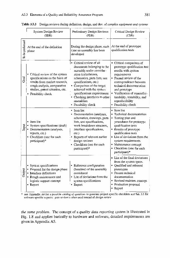
Table A3.3 Design reviews during definition, design, and dev. of complex equipment und Systems
System Design Review W R )
At the end of the definition phase
Critical review of the system specifications on the basis of results from market research, rough analysis, comparative studies, patent situation, etc. Feasibility check
Item list System specifications (draft) Documentation (analyses, reports, etc.) Checklists (one for each participant)*
System specifications - Proposal for the design phase Interface definitions Rough maintenance and logistic support concept Report
Preliminary Design Reviews (PDR)
During the design phase, each time an assembly has been developed
Critical review of all documents belonging to the assembly under consider- ation (calculations, schematics, parts lists, test specifications, etc.) Comparison of the target achieved with the system specifications requirements Checking interfaces to other assemblies Feasibility check
Item list Documentation (analyses, schematics, drawings, parts lists, test specifications, work breakdown structure, interface specifications, etc.) Reports of relevant earlier design reviews Checklists (one for each participant)*
Reference configuration (baseline) of the assembly considered List of deviations from the system specifications Report
Critical Design Review (CDR)
At the end of prototype qualification tests
Cntical comparison of prototype qualification tesi results with system requirements Formal review of the correspondence between technical documentation and prototype Verification of mannufac- turability, testability, and reproducibility Feasibility check
Item list Technical documentation Testing plan and procedures for prototype qualification tests Results of prototype qualification tests List of deviations from the system requirements Maintenance concept Checklists (one for each participant)"
List of the final deviations from the system specs. Qualified and released Prototypes Frozen technical documentation Revised mainten. concept Production proposal Report
See Appendix A4 for a possible catalog of qucstions to generatc project specific checklists and Tab. 5.5 for software specific aspects; gate review is often uscd instead of design review
the same problem. The concept of a quality data reporting system is illustrated in Fig. 1.8 and applies basically to hardware and software, detailed requirements are given in Appendix A5.

382 A3 Definition and Realization of Quality and Reliability Requirements
The quality and reliability assurance program should for instance answer the following questions:
1. How is the collection of defect and failure data carried out? At which project phase is started with?
2. How are defects and failures analyzed? 3. Who carries out corrective actions? Who monitors their realization? Who
checks the final configuration? 4. How is evaluation and feedback of quality and reliability data organized?
5. Who is responsible for the quality data reporting system? Does production have their own locally limited version of such a system? How does this Systems interface with the company's quality data reporting system?
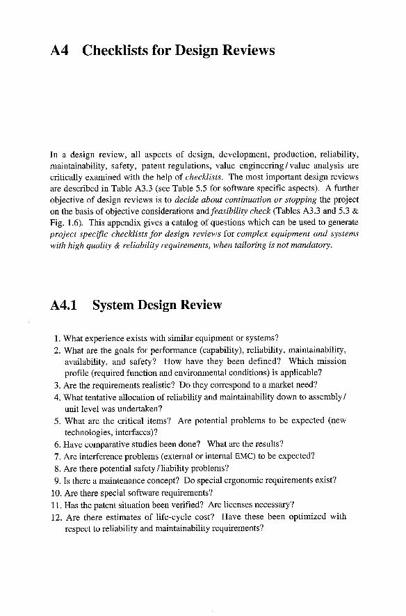
Checklists for Design Reviews
In a design review, all aspects of design, development, production, reliability, maintainability, safety, patent regulations, value engineeringlvalue analysis are critically examined with the help of checklists. The most important design reviews are described in Table A3.3 (see Table 5.5 for software specific aspects). A further objective of design reviews is to decide about continuation or stopping the project on the basis of objective considerations and feasibility check (Tables A3.3 and 5.3 &
Fig. 1.6). This appendix gives a catalog of questions which can be used to generate project specific checklists for design reviews for complex equipment und systems with high quality & reliability requirements, when tailoring is not mandatory.
A4.1 System Design Review
1. What experience exists with similar equipment or systems? 2. What are the goals for performance (capability), reliability, maintainability,
availability, and safety? How have they been defined? Which mission profile (required function and environmental conditions) is applicable?
3. Are the requirements realistic? Do they correspond to a market need? 4. What tentative allocation of reliability and maintainability down to assembly 1
unit level was undertaken? 5. What are the critical items? Are potential problems to be expected (new
technologies, interfaces)? 6. Have comparative studies been done? What are the results? 7. Are interference problems (external or internal EMC) to be expected? 8. Are there potential safety Iliability problems? 9.1s there a maintenance concept? Do special ergonomic requirements exist?
10. Are there special software requirements? 1 1. Has the patent situation been verified? Are licenses necessary? 12. Are there estimates of life-cycle cost? Have these been optimized with
respect to reliability and maintainability requirements?
3 84 A4 Checklists for Design Reviews
13. 1s there a feasibility study? Where does the competition stand? Has devel- opment risk been assessed?
14. 1s the project time schedule realistic? Can the system be marketed at the right time?
15. Can supply problems be expected during production ramp-up?
A4.2 Preliminary Design Reviews
a) General
1. 1s the assembly / m i t under consideration a new development or only a change/modification? Can existing items (e.g. sub assemblies) be used?
2.1s there experience with similar assembly /mit? What were the problems? 3.1s there redundancy hardware and / or software? 4. Have customer and market demands changed since the beginning of
development? Can individual requirements be reduced? 5. Can the chosen solution be further simplified? 6. Are there patent problems? Do licenses have to be purchased? 7. Have expected cost and deadlines been met? Were value engineering used?
b) Performance Parameters
1. How have been defined the main performance Parameters of the assembly / unit under consideration? How was their fulfillment verified (calculations, simulation, tests)?
2. Have worst case situations been considered in calculations / simulations? 3. Have interference problems (EMC) been solved? 4. Have applicable standards been observed during design and development? 5. Have interface problems with other assemblies Iunits been solved? 6. Have Prototypes been adequately tested in laboratory?
C) Environmental Conditions
1. Have environmental conditions been defined? As a function of time? Were these consequently used to determine component operating conditions?
2. How were EMC interference been determined? Has his influence been taken into account in worst case calculation/ simulation?

A4.2 Preliminary Design Reviews 385
d) Components and Materials
1. Which components and materials do not appear in the preferred lists? For what reasons? How were these components and materials qualified?
2. Are incoming inspections necessary? For which components and materials? How / Who will they be performed?
3. Which components and materials were screened? How / Who will screening be performed?
4. Are suppliers guaranteed for series production? 1s there at least one second source for each component and material? Have requirements for quality, reliability, and safety been met?
5. Are obsolescence problems to be expected? How will they be solved?
e) Reliability
See Table 2.8.
f) Maintainability
See Table 4.3.
g) Safety
1. Have applicable standards concerning accident prevention been observed? 2. Has safety been considered with regard to external causes (natural
catastrophe, sabotage, etc.)? 3. Has a FMEAIFMECA or similar cause-to-effects analysis been performed?
Are there failure modes with critical or even catastrophic consequence? Can these be avoided? Have all single-point failures been identified? Can these be avoided?
4. Has a fail-safe analysis been performed? What were the results? 5. What safety tests are planned? Are they sufficient? 6. Have safety aspects been dealt with adequately in the documentation?
h) Human Factors, Ergonomics
1. Have operating and maintenance sequences been defined with regard to the training level of Operators and maintenance personnel?
2. Have ergonomic factors been taken into account by defining operating sequences?
3. Has the man-machine interface been sufficiently considered?
386 A4 Checklists for Design Reviews
i) Standardization
1. Have standard components and materials been used wherever possible? 2. Has items exchangeability been considered during design and construction?
j) Configuration
1. 1s the technical documentation (schematics, drawings, etc.) complete, error- free, and does it reflect the present state of the project?
2. Have all interface problems between assemblies Iunits been solved? 3. Can the technical documentation be frozen and considered as reference
documentation (baseline)? 4. How is compatibility (upward andlor downward) assured?
k) Production and Testing
1. Which qualification tests are foreseen for prototypes? Have reliability, maintainability, and safety aspects been considered sufficiently in these tests?
2. Have all questions been answered regarding manufacturability, testability, and reproducibility?
3. Are special production processes necessary? Were they qualified? What were the results?
4. Are special transport, packaging, or storage problems to be expected?
A4.3 Critical Design Review (System Level)
a) Technical Aspects
1. Does the documentation allow an exhaustive and correct interpretation of test procedures and results? Has the technical documentation been frozen? Has conformance with present hardware and software been checked?
2. Are test specifications and procedures complete? In particular, are conditions for functional, environmental, reliability, and safety tests clearly defined?
3. Have fault criteria been defined for critical parameters? 1s an indirect measurement planned for those parameters which cannot be measured accurately enough during tests?
4. Has a representative mission profile, with the corresponding required function, been clearly defined for reliability tests?

A4.3 Cntical Design Review (System Level) 387
5. Have test criteria for maintainability been defined? Which failures were simulated / introduced? How have personnel and material conditions been fixed?
6. Have test criteria for safety been defined (accident prevention and technical safety)?
7. Have ergonornic aspects been checked? How? 8. Can packaging, transport and Storage cause problems? 9. Have defects and failures been systematically analyzed (mode, cause, effect)?
Has the usefulness of corrective actions been verified? How? Also with respect to cost?
10. Have all deviations been recorded? Can they be accepted? 11. Does the system still satisfy customer/market needs? 12. Are manufacturability and reproducibility guaranteed within the framework
of a production environment?
b) Formal Aspects
1.1s the technical documentation complete? 2. Has the technical documentation been checked for correctness?
For coherency? 3.1s uniqueness in numbering guaranteed? Even in the case of changes? 4.1s hardware labeling appropriate? Does it satisfy production and maintenance
requirements? 5. Has conformance between Prototype and documentation been checked? 6. 1s the maintenance concept mature? Are spare parts having a different
change Status fully interchangeable? 7. Are production tests sufficient from today's point of view?
A5 Requirements for Quality Data Reporting Systems
A quality data reporting System is a system to collect, analyze, and correct all defects and failures occurring during production and testing of an item, as well as to evaluate and feedback the corresponding quality and reliability data (Fig. 1.8). The system is generally computer-aided. Analysis of failures and defects must go back to the root cause in order to determine the most appropriate action necessary to avoid repetition of the same problern. The quality data reporting system applies basically to hardware and software. It should remain active during the operating phase, at least for the warranty time. This appendix summarizes the requirements for a computer-aided quality data reporting system for complex equipment and systems.
a) General Requirements
1. Up-to-dateness, completeness, and utility of the delivered information must be the primary concern (best compromise).
2. A high level of u s a b i l i ~ (user friendliness) and minimal manual intervention should be a goal.
3. Procedures and responsibilities should be clearly defined (several levels depending upon the consequence of defects or failures).
4. The system should be flexible and easily adaptable to new needs.
b) Requirements Relevant to Data Collection
1. All data concerning defects and failures (relevant to quality, reliability, maintainability, and safety) have to be collected, from the begin of Prototype qualification tests to (at least) the end of the warranty time.
2. Data collection forms should be preferably 8" X 11 " or A4 format be project-independent and easy to fill in
ensure that only the relevant information is entered and answers the questions: what, where, when, why, and how?
A5 Requirements for Quality Data Reporting Systems 389
have a separate field (20-30%) for free-format input for comrnents (requests for analysis, logistic information, etc.), these comments do not need to be processed and should be easily separable from the fixed portion of the form.
3. Description of the Symptom (mode), analysis (cause, effect), and corrective action undertaken should be recorded in clear text and coded at data entry by trained personnel.
4. Data collection can be carried out in different ways at a single reporting location (adequate for simple problems which can be solved directly at the reporting location) from different reporting locations which report the fault (defect or failure), analysis result, and corrective action separately.
Operating reliability, maintainability, or logistic data can also be reported.
5. Data collection forms should be entered into the Computer daily (on line if possible), so that corrective actions can be quickly initiated (for field data, a weekly or monthly entry can be sufficient for many purposes).
C) Requirements for Analysis
1. The cause should be found for each defect or failure at the reporting location, in the case of simple problems by a fault review board, in critical cases.
2. Failures (and defects) should be classified according to
mode - sudden failure (short, Open, fracture, etc.) - gradual failure (drift, wearout, etc.) - intermittent failures, others if needed cause - intrinsic (inherent weaknesses, wearout, or some other intrinsic cause) - extrinsic (systernatic failure, i.e. misuse, mishandling, design, or manuf. failure) - secondary failure effect - irrelevant - partial failure - cornplete failure - critical failure (safety problern).
3. Consequence of the analysis (repair, rework, change, scraping) must be reported.
d) Requirements for Corrective Actions
1. Every record is considered pending until the necessary corrective action has been successfully completed and certified.
2. The quality data reporting system must monitor all corrective actions.

A5 Requirements for Quality Data Reporting Systems 390
3. Procedures and responsibilities pertaining to corrective action have to be defined (simple cases usually solved by the reporting location).
4. The reporting location must be informed about a completed corrective action.
e) Requirements Related to Data Processing, Feedback, and Storage
1. Adequate coding must allow data compression and simplify data processing.
2. Up-to-date information should be available on-line. 3. Problem-dependent and periodic data evaluation must be possible.
4. At the end of a project, relevant information should be stored for comparative investigations.
f) Requirements Related to Compatibility with other Software Packages
1. Compatibility with company's configuration management and data banks should be assured.
2. Data transfer with the following external software packages should be assured important reliability data banks quality data reporting systems of subsidiary companies quality data reporting systems of large contractors.
The effort required for implementing a quality data reporting system as described above can take 5 to 10 man-years for a medium-sized company. Competence for operation and maintenance of the quality data reporting system should be with the company's quality and reliability assurance department. The priority for the realization of corrective actions is project specific and should be fixed by the project manager. Major problems (defects and failures) should be discussed periodically by a fault review board chaired by the company's quality and reliability assurance manager, which should have, in critical cases defined in the company's quality assurance handbook, the competence to take golnogo decisions.
Basic Probability Theory
In many practical situations, experiments have a random outcome, i.e., the results cannot be predicted exactly, although the same experiment is repeated under identical conditions. Examples in reliability engineering are failure-free time of a given System, repair time of equipment, inspection of a given item during produc- tion, etc. Experience shows that as the number of repetitions of the same experiment increases, certain regularities appear regarding the occurrence of the event consid- ered. Probability theory is a mathematical discipline which investigates the laws describing such regularities. The assumption of unlimited repeatability of the same experiment is basic to probability theory. This assumption permits the introduction of the concept of probability for an event starting from the properties of the relative frequency of its occurrence in a long series of trials. The axiomatic theory ofproba- bility, introduced 1933 by A.N. Kolmogorov [A6.10], brought probability theory to a mathematical discipline. In reliability analysis, probability theory allows the investigation of the probability that a given item will operate failure-free for a stated period of time under given conditions, i.e. the calculation of the item's reliability on the basis of a mathematical model. The d e s necessary for such calculations are presented in Sections A6.1- A6.4. The following sections are devoted to the con- cept of random variables, necessary to investigate reliability as a function of time and as a basis for stochastic processes (Appendix A7) and mathematical statistics (Appendix Ag). This appendix is a compendium of probability theory, consistent from a mathematical point of view but still with reliability engineering applications in mind. Selected examples illustrate the practical aspects.
A6.1 Field of Events
As introduced 1933 by A.N. Kolmogorov [A6.10], the mathematical model of an experiment with random outcome is a triplet [Q, F , Pr], also called probability space. & is the sample space, F the event field, and Pr the probability of each element of F . is a Set containing as elements all possible outcomes of the experi- ment considered. Hence & = {i,2, 3, 4, 5, 6) if the experiment consists of a single throw of a die, and SZ = [O, W) in the case of failure-free times of an item. The
392 A6 Basic Probability Theory
elements of SZ are called elementary events and are represented by W. If the logical Statement "the outcome of the experiment is a subset A of SZ" is identified with the subset A itself, combinations of Statements become equivalent to operations with subsets of SZ. If the sample space SZ is finite or countable, a probability can be assigned to every subset of SZ. In this case, the event field F contains all subsets of SZ and all combinations of them. If L2 is continuous, restrictions are necessary. The eventfield F is thus a system of subsets of SZ to each of which a probability has been assigned according to the situation considered. Such a field is called a o-field ( o-algebra) and has the following properties:
1. SZ is an element of g . 2. If A is an element of F, its complement Ä is also an element of F . 3. If Al , A2, ... are elements of g , the countable union Al U A2 U ... is also an
element of F.
From the first two properties it follows that the empty set 0 belongs to F . From the last two properties and De Morgan's law one recognizes that the countable intersection Al n A2 n . . . also belongs to F. In probability theory, the elements of
are called (random) events. The most important operations on events are the union, the intersection, and the complement:
1. The union of a finite or countable sequence Al , A2, ... of events is an event which occurs if at least one of the events Al , A2, . . . OCCU~S; it will be denoted by Al u A 2 U . . . orby U i A i .
2. The intersection of a finite or countable sequence Al, A2, . . . of events is an event which occurs if each one of the events Al, A2, . . . occurs; it will be denotedby Al n A 2 n... orby f l iA i .
3. The complement of an event A is an event which occurs if and only if A does - - notoccur;itisdenotedby A , A = { w : w @ A } = Q \ A , A U Ä = Q , ~ n Ä = 0 .
Important properties of set operations are:
Commutativelaw : A u B = B U A ; A n B = B n A
Associativelaw : A u ( B u C ) = ( A u B ) u C ; A n ( B n C ) = ( A n B ) n C
Distributivelaw : A u ( B n C ) = ( A u B ) n ( A u C ) ; A n ( B u C ) = ( A n B ) u ( A n C )
Complementlaw : ~ n Ä = 0 ; A U Ä = Q
Idempotentlaw : A u A = A ; A n A = A De Morgan's law : A U B = A n B; A n B = A U B
= - Iden t i t y l aw : A = A ; A u ( A n B ) = A u B .
The sample space B is also called the sure event and 0 is the impossible event. The events Al , A2, . . . are mutually exclusive if Ai n Aj = $3 holds for any i # j . The events A and B are equivalent if either they occur together or neither of them occur, equivalent events have the same probability. In the following, events will be mainly enclosed in braces { } .
A6.2 Concept of Probability
A6.2 Concept of Probability
Let us assume that 10 (random) samples of size n = 100 were taken from a large and homogeneous lot of populated printed circuit boards (PCBs), for incoming inspection. Examination yielded the following results:
Sample number: 1 2 3 4 5 6 7 8 9 1 0
No. of defective PCBs: 6 5 1 3 4 0 3 4 5 7
For 1000 repetitions of the "testing a PCB" experiment, the relative frequency of the occurrence of event {PCB defective) is
It is intuitively appealing to consider 0.038 as the probability of the event {PCB defective}. As shown below, 0.038 is a reasonable estimation of this probability (on the basis of the experimental observations made).
Relative frequencies of the occurrence of events have the property that if n is the number of trial repetitions and n(A) the number of those trial repetitions in which the event A occurred, then
is the relative frequency of the occurrence of A, and the following d e s apply:
1. R1: j n ( A ) 2 0 .
2. R2: &(Q) = 1.
3. R3: if the events Al, . . ., Am are mutually exclusive, then n(Al U ... U Am) = n(Al) + ... + n(Am) and ;,(Al U ... UA,) = f i n ( ~ i ) + ... + &(A&.
Experience shows that for a second group of n trials, the relative frequency F,(A) can be different from that of the first group. j,(A) also depends on the number of trials n. On the other hand, experiments have confirmed that with increasing n, the value & ( A ) converges toward a fixed value p(A) , see Fig. A6.1 for an example. It therefore seems reasonable to designate the limiting value p ( A ) as the probability P ~ { A ) of the event A , with ; J A ) as an estimate of P ~ { A ) . Although intuitive, such a definition of probability would lead to problems in the case of continuous (non-denumerable) sample spaces.
Since Kolmogorov's work [A6.10], the probability P ~ { A ) has been defined as a function on the event field F of subsets of 8. The following axioms hold for this function:
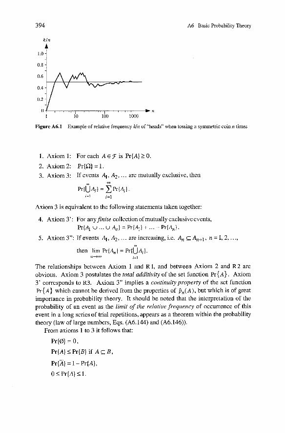
A6 Basic Probability Theory
kln
0.8
Figure A6.1 Example of relative frequency Wn of "heads" when tossing a symmetric coin n times
1. Axiom 1: Foreach A € F i s Pr{A}20.
2. Axiom 2: Pr{Q) = 1.
3. Axiom 3: If events Al, A2, . . . are mutually exclusive, then
Axiom 3 is equivalent to the following Statements taken together:
4. Axiom 3' : For any finite collection of mutually exclusive events, Pr{A1 U ... U An} = Pr{AI) + ... + Pr{A,}.
5. Axiom 3": If events Al, A2, . . . are increasing, i.e. An L An+1, n = 1,2, . . ., m
then lim Pr(An} = pr{UAi1. n-3- i= l
The relationships between Axiom 1 and R 1, and between Axiom 2 and R 2 are obvious. Axiom 3 postulates the total additivity of the set function P ~ { A ) . Axiom 3' corresponds to R3. Axiom 3" implies a continuityproperty of the set function P ~ { A ) which cannot be derived from the properties of $,(A), but which is of great importance in probability theory. It should be noted that the interpretation of the probability of an event as the limit of the relative frequency of occurrence of this event in a long series of trial repetitions, appears as a theorem within the probability theory (law of large numbers, Eqs. (A6.144) and (A6.146)).
From axioms 1 to 3 it follows that:
Pr{@} = 0 ,
Pr{A}<Pr{B} if A c B,
~r {Ä} = 1 - Pr {A} ,
A6.2 Concept of Probability 395
When modeling an experiment with random outcome by means of the probability space [Q, F, Pr], the difficulty is often in the determination of the probabilities P ~ { A ) for every A E g. The structure of the experiment can help here. Beside the statistical probability, defined as the limit for n -+ - of the relative frequency k l n, the following d e s can be used if one assumes that all elementary events o have the same chance of occurrence:
1. Classical probability (discrete uniform distribution): If Q is a finite set and A
a subset of LI, then
number of elements in A Pr{A} =
number of elements in Q
number of favorable outcomes Pr(A} =
number of possible outcomes
2. Geometrie probability (spatial uniform distribution): If Q is a Set in the plane R~ of area Q and A a subset of Q, then
area of A Pr{A} =
area of LI
It should be noted that the geometric probability can also be defined if Q is a part of the Euclidean space having a finite area. Examples A6.1 and A6.2 illustrate the use of Eqs. (A6.2) and (A6.3).
Example A6.1 From a shipment containing 97 good and 3 defective ICs, one IC is randomly selected. What is the probability that it is defective?
Solution From Eq. (A6.2),
3 Pr{IC defective] = -
100
Example A6.2 Maurice and Matthew wish to meet between 8:00 and 9:00 a.m. according to the following d e s : 1) They come independently of each other and each will wait 12 minutes. 2) The time of arrival is equally distributed between 8:00 and 9:00 a.m. What is the probability that they will meet?
Solution Arrival of Matthew
Equation (A6.3) can be applied and leads to, see graph, A
0.8. 0.8 1-2-
PrIMatthew meets Maurice) = = 0.36. 1
396 A6 Basic Probability Theory
Another way to determine probabilities is to calculate them from other probabilities which are known. This involves paying attention to the structure of the experiment and application of the d e s of probability theory (Appendix A6.4). For example, the predicted reliability of a system can be calculated from the reliability of its elements and the system's structure. However, there is often no alternative to determining probabilities as the limits of relative frequencies, with the aid of statistical methods (Appendices A6.1 I and A8).
A6.3 Conditional Probability, Independence
The concept of conditional probability is of great importance in practical applications. It is not difficult to accept that the information "event A has occurred in an experiment" can modify the probabilities of other events. These new probabilities are defined as conditional probabilities and denoted by Pr{B I A } . If for example A B, then Pr{B I A } = 1, which is in general different from the original unconditional probability Pr( B) . The concept of conditional probability Pr{B I A ) of the event B under the condition "event A has occurred", is introduced here using the properties of relative frequency. Let n be the total number of trial repetitions and let n ( A ) , n( B) , and n ( A n B ) be the number of occurrences of A, B and A n B, respectively, with n ( A ) > 0 assumed. When considering only the n ( A ) trials (trials in which A occurs), then B occurs in these n ( A ) trials exactly when it occurred together with A in the original trial series, i.e. n( A n B ) times. The relative frequency of B in the trials with the information "A has occurred" is therefore
Equation (A6.4) leads to the following definition of the conditional probability Pr(B I A } of an event B under the condition A, i.e. assuming that A has occurred,
From Eq. (A6.5) it follows that
Pr{A n B} = Pr{A} Pr{B I A} = Pr{B} Pr{A I B}. (A6.6)
Using Eq. (A6.5), probabilities Pr{B I A } will be defined for all B E F . Pr{B I A } is
A6.3 Conditional Probability, Independence 397
a function of B which satisfies Axioms 1 to 3 of Appendix A6.2, obviously with Pr{A I A ) = 1 . The information "event A has occurred" thus leads to a new probability space [ A , F A , PrA] , where F A consists of events of the form A n B, with B E F and P r A { B } = P r ( B I A ) , seeExampleA6.5.
It is reasonable to define the events A and B as independent if the information "event A has occurred" does not influence theprobability of the occurrence of event B, i.e. if
However, when considering Eq. (A6.6), another definition, with symmetry in A and B is obtained, where P r { A ] > 0 is not required. Two events A and B are independent if and only if
Pr {A n B) = Pr {A} Pr {B}. (A6.8)
The events A l , ..., An are (stochastically) independent if for each k (1 < k 5 n) and any selection of distinct i l , ..., ik E {i, ..., n)
holds.
A6.4 Fundamental Rules of Probability Theory
The probability calculation of event combinations is based on the fundamental d e s of probability theory introduced in this section.
A6.4.1 Addition Theorem for Mutually Exclusive Events
The events A and B are mutually exclusive if the occurrence of one event excludes the occurrence of the other, formally A n B = 0. Considering a component which can fail due to a short or an Open circuit, the events
failure occurs due to a short circuit
and
failure occurs due to an Open circuit
are mutually exclusive. Application of Axiom 3 (Appendix A6.2) leads to
398 A6 Basic Probability Theory
Pr{A U B) = Pr(A} + Pr (B}. (A6.10)
Equation (A6.10) is considered a theorem by tradition only; indeed, it is a particular case of Axiom A3 in Appendix A6.2.
Example A6.3
A shipment of 100 diodes contains 3 diodes with shorts and 2 diodes with Opens. If one diode is randomly selected from the shipment, what is the probability that it is defective?
Solution
From Eqs. (A6.10) and (A6.2),
If the events A l , A2 , . . . are mutually exclusive ( A i n A j = 0 for all i # j , they are also totally exclusive. According to Axiom 3 it follows that
A6.4.2 Multiplication Theorem for Two Independent Events
The events A a n d B a r e independent if the information about occurrence (or nonoccurrence) of one event has no influence on the probability of occurrence of the other event. In this case Eq. (A6.8) applies
Example A6.4 A system consists of two elements E1 and E2 necessary to fulfill the required function. The failure of one element has no influence on the other. R1 = 0.8 is the reliability of E1 and R2 = 0.9 is that of E2 . What is the reliability RS of the system?
Solution
Considering the assumed independence between the elements E1 and E2 and the definition of R1, R2 , and RS as R1 = Pr{EI fulfills the required function] , R2 = Pr [E2 fulfills the required function] , and RS = Pr[El fulfills the required function n E2 fulfills the required function) , one
obtains from Eq. (A6.8)
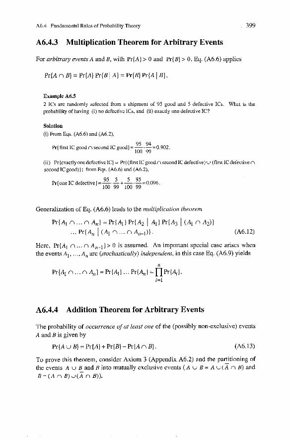
A6.4 Fundamental Rules of Probability Theory
A6.4.3 Multiplication Theorem for Arbitrary Events
For arbitrary events A and B, with Pr{A} > 0 and Pr{B} > 0, Eq. (A6.6) applies
Pr{A n B} = Pr{A} Pr{B I A} = Pr{B} Pr{A I B}.
Example A6.5 2 ICs are randomly selected from a shipment of 95 good and 5 defective ICs. What is the probability of having (i) no defective ICs, and (ii) exactly one defective IC?
Solution (i) From Eqs. (A6.6) and (A6.2),
95 94 Pr{ first IC good n second IC good) = - .- = 0.902.
100 99
(ii) PrIexactly one defective IC] = Pr{(first IC good n second IC defective) U (first IC defective n second IC good)) ; from Eqs. (A6.6) and (A6.2),
Generalization of Eq. (A6.6) leads to the multiplication theorem
Here, Pr{Al n .. . n } > 0 is assumed. An important special case arises when the events A l , ..., An are (stochastically) independent, in this case Eq. (A6.9) yields
A6.4.4 Addition Theorem for Arbitrary Events
The probability of occurrence of at least one of the (possibly non-exclusive) events A and B is given by
Pr{A U B) = Pr {A} + Pr{B} - Pr{A n B}. (A6.13)
To prove this theorem, consider Axiom 3 (Appendix A6.2) and the partitioning of the events A u B and B into mutually exclusive events ( A U B = A u (Ä n B) and B = ( A n B ) u ( Ä n B)).
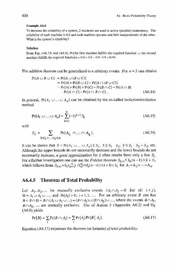
400 A6 Basic Probability Theory
Example A6.6 To increase the reliability of a System, 2 machines are used in active (parallel) redundancy. The reliability of each machine is 0.9 and each machine operates and fails independently of the other. What is the system's reliability?
Solution From Eqs. (A6.13) and (A6.8), Pr{the first machine fulfills the required function U the second machine fulfills the required function] = 0.9 + 0.9 - 0.9 .0.9 = 0.99.
The addition theorem can be generalized to n arbitrary events. For n = 3 one obtains
Pr{A U B U C} = Pr{A U ( B U C ) ) = Pr{A} + Pr{B U C} - Pr{A n ( B U C ) ) = Pr{A} + Pr{B} + Pr{C} - Pr{B n C} - Pr{A n B] - Pr{A n C} + Pr{A n B n C ) . (A6.14)
In general, Pr{Al U .. . U An) can be obtained by the so-called inclusion/exclusion method
n Pr{Al U ... U An) = x ( - l ) k + l ~ k
k=l
with
It can be shown that S = Pr{A1 U ... U A n } < S I , S $ . S1 - S 2 , S 5 SI - S 2 + S 3 , etc. Although the upper bounds do not necessarily decrease and the lower bounds do not necessarily increase, a good approximation for S often results from only a few Si. For a further investigation one can use the Frkchet theorem Sk„< Sk ( n - k ) 1 ( k + I), which follows from s ~ + ~ = s ~ ( ~ : ~ ) /(i() =sk(n - k ) / ( k + 1)c sk for A1=A2=.. . =An.
A6.4.5 Theorem of Total Probability
Let A l , A2, ... be mutually exclusive events (Ai n Aj = 0 for all i # j), 52 = Al U A2 U ..., and Pr{Ai) > 0, i = 1, 2, ... . For an arbitrary event B one has B = B n Q = B n ( A l u A 2 U ...) = ( B n A 1 ) u ( B n A 2 ) u ..., where the events B n A l , B n A2, . . . are mutually exclusive. Use of Axiom 3 (Appendix A6.2) and Eq. (A6.6) yields
Equation (A6.17) expresses the theorem (or formula) of total probability.
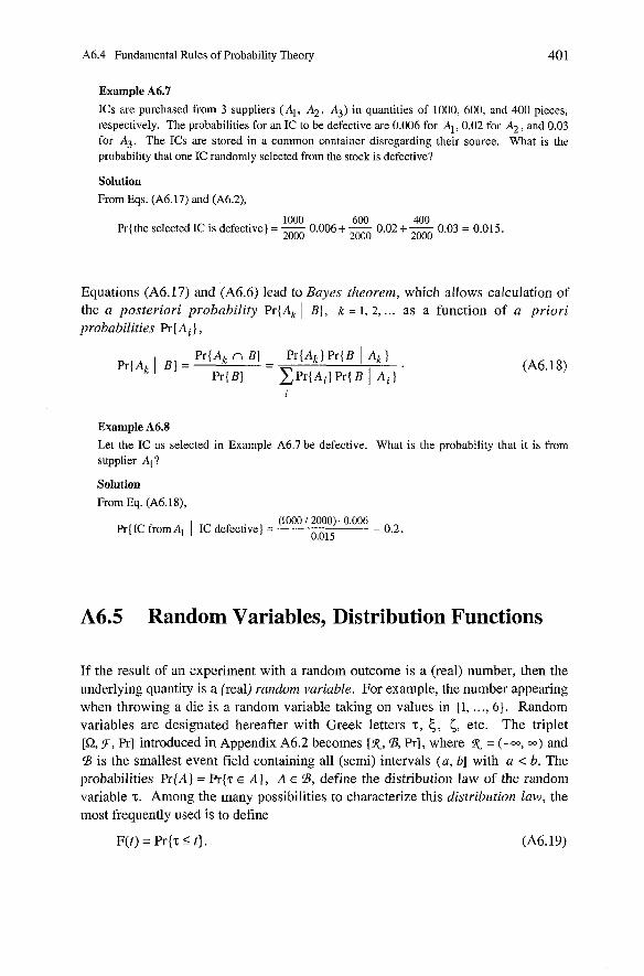
A6.4 Fundamental Rules of Probability Theory 40 1
Example A6.7 ICs are purchased from 3 suppliers (Al, A2, A3) in quantities of 1000, 600, and 400 pieces, respectively. The probabilities for an IC to be defective are 0.006 for Al, 0.02 for A2, and 0.03 for A3. The ICs are stored in a common container disregarding their source. What is the probability that one IC randomly selected from the stock is defective?
Solution From Eqs. (A6.17) and (A6.2),
1000 600 400 Pr{the selected IC is defective} = - 0.006 + - 0.02 + - 0.03 = 0.015.
2000 2000 2000
Equations (A6.17) and (A6.6) lead to Bayes theorem, which allows calculation of the a posteriori probability Pr{& I B}, k = 1, 2, ... as a function of a priori probabilities Pr{Ai},
Example A6.8
Let the IC as selected in Example A6.7 be defective. What is the probability that it is from supplier Al?
Solution From Eq. (A6.18),
(1000 12000). 0.006 Pr{IC from Al I IC defective) = = 0.2.
0.015
A6.5 Random Variables, Distribution Functions
If the result of an experiment with a random outcome is a (real) number, then the underlying quantity is a (real) random variable. For example, the number appearing when throwing a die is a random variable taking on values in (1, . . ., 6}. Random variables are designated hereafter with Greek letters T, 5, 5, etc. The triplet [Q, F, Pr] introduced in Appendix A6.2 becomes [ K , 23, Pr], where = (-W, -) and B is the smallest event field containing all (semi) intervals ( U , b] with a < b. The probabilities Pr{A] = Pr{z E Al, A E B, define the distribution law of the random variable T. Among the many possibilities to characterize this distribution law, the most frequently used is to define
F(t) = Pr{z 5 t} . (A6.19)
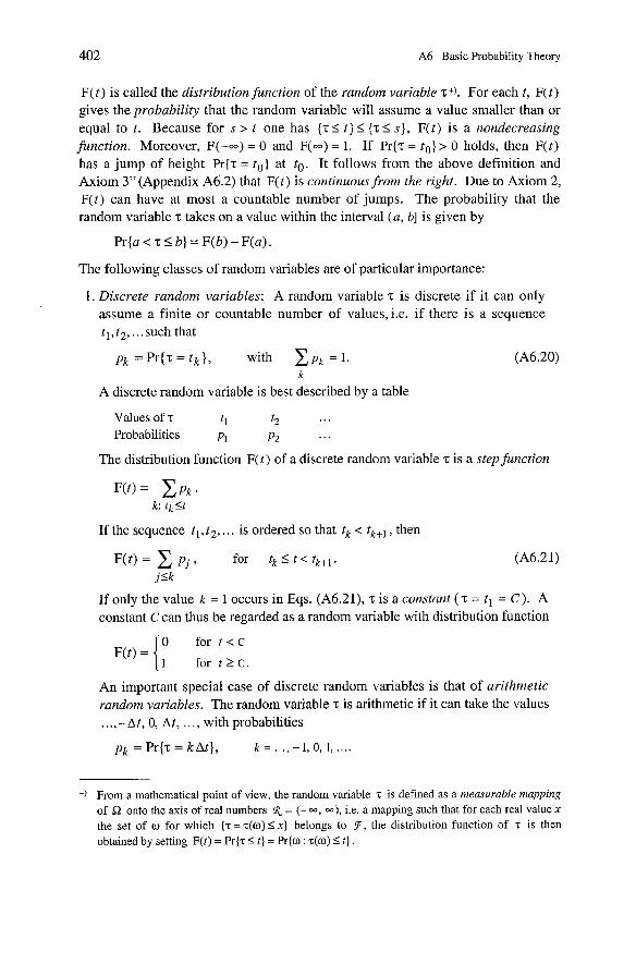
402 A6 Basic Probability Theory
F( t ) is called the distributionfunction of the random variable T+). For each t, F( t ) gives the probability that the random variable will assume a value smaller than or equal to t . Because for s > t one has {T 2 t } 2 {T 2 s ] , F(t) is a nondecreasing function. Moreover, F(--) = 0 and F(..) = 1. If Pr(z = t o } > 0 holds, then F(t) has a jump of height Pr{z = t o ) at t ~ . It follows from the above definition and Axiom 3" (Appendix A6.2) that F(t) is continuous from the right. Due to Axiom 2, F(t) can have at most a countable number of jumps. The probability that the random variable z takes on a value within the interval ( U , b] is given by
The following classes of random variables are of particular importance:
1. Discrete random variables: A random variable z is discrete if it can only assume a finite or countable number of values, i.e. if there is a sequence t l , t z , ... such that
pk = Pr{z = t k } , with zp, = 1. (A6.20) k
A discrete random variable is best described by a table
Values of T t 1 t2
Probabilities p, P2
The distribution function F(t) of a discrete random variable z is a stepfunction
If the sequence t i , t z , . . . is ordered so that tk < tk+l, then
F(t) = C pj , for tk 2 t < tk+i. jSk
If only the value k = 1 occurs in Eqs. (A6.21), z is a constant ( T = tl = C ) . A constant C can thus be regarded as a random variable with distribution function
0 for t < C F(t) =
1 f o r t 2 C .
An important special case of discrete random variables is that of arithmetic random variables. The random variable z is arithmetic if it can take the values ...,- At, 0, At, . . . , with probabilities
+) From a mathematical point of view, the random variable T is defined as a measurable mapping of 52 onto the axis of real numbers = (-W, W), i.e. a mapping such that for each real value X
the Set of o for which {T = ~ ( o ) S X } belongs to !F, the distribution function of T is then obtained by Setting F(t) = Pr{z 5 t } = Pr@ : z(w) 5 t } .
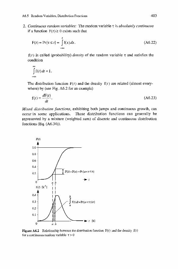
A6.5 Random Variables, Distribution Functions 403
2. Continuous random variables: The random variable z is absolutely continuous if a function F(t) 2 0 exists such that
f ( t ) is called (probability) density of the random variable z and satisfies the condition
The distribution function F(t) and the density f ( t ) are related (almost every- where) by (see Fig. A6.2 for an example)
Mixed distribution functions, exhibiting both jumps and continuous growth, can occur in some applications. These distribution functions can generally be represented by a mixture (weighted sum) of discrete and continuous distribution functions (Eq. (A6.34)).
Figure A6.2 Relationship between the distribution function F(t) and the density f ( t ) for a continuous random variable T > 0
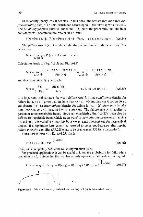
404 A6 Basic Probability Theory
In reliability theory, T > O denotes (in this book) the failure-free time @ilure- free operating time) of an item,distributed according to F(t) = Pr(7 I t} with F(0) = 0. The reliability function (survival function) R(t) gives the probability that the item considered will operate failure-free in (0, t]; thus,
F(t) = Pr{z I t}, R(t) = Pr{z > t} = 1 - F(t) , z > 0, F(O)=O, R(O)= 1. (A6.24)
The failure rate h(t) of an item exhibiting a continuous failure-free time T is defined as
Calculation leads to (Eq. (A6.5) and Fig. A6.3)
1 P r { t < ~ < t + & r i ~ > t ] 1 Pr{t < T 5 t + St} h(t) = lim - . = lim - .
6t.10 6t Pr(z > t} 6t50 6t Pr{z > t}
and thus, assuming F( t ) derivable,
f( t) dR(t) l d t h(t) = - = - -, 1 - F(t) R( t)
It is important to distinguish between failure rate h(t), as conditional density for failure in (t, t + St] given that the item was new at t=O and has not failed in (0, t], and density f(t), as unconditional density for failure in (t , t + St] given only that the item was new a t t=O (assumed with F(0) = 0). The failure rate h ( t ) applies in particular to nonrepairable items. However, considering Eq. (A6.25) it can also be defined for repairable items which are as-good-as-new aper repair (renewal), taking instead of t the variable x starting by x = 0 a t euch renewal (as for interarrival times). If a repairable item cannot be restored to be as-good-as-new after repair, failure intensity z (t) (Eq. (A7.228)) has to be used (see p. 356 for a discussion).
Considering R(0) = 1, Eq. (A6.25) yields
Thus, h ( t ) completely define the reliability function R(t). For practical applications it can be useful to know the probability for failure-free
operation in (0, t] given that the item has already operated a failure-free time xo > O f + X 0
(A6.27) pr{T> t + x 0 I w x o } = ~ ( t , x o ) = ~ ( t + x ~ ) / ~ ( x ~ ) = e x o
Figure A6.3 Visual aid to compute the failure rate h(t) ( h(x) for interarrival times)
A6.5 Random Variables, Distribution Functions 405
From Eq. (A6.27) it follows that 00
- dR(t,xo)ldt = ( t x o ) = ( x 0 ) and E[T-xo / r >xo]=[ R(x)&/ R(xo).
R ( t , x o ) (A6.28)
From the left-hand side of Eq. (A6.28) one recognizes that the conditional failure rate h(t,xo) at time t given that the item has operated failure-free a time xo is the failure rate at time t + xo (=h for h(x)=h). This leads to the concept of bad-as-old used in some considerations on repairable Systems [6.3] (see also p. 497).
Important conclusions as to the aging behavior of an item can be drawn from the shape of its failure rate. For h(t) nondecreasing, it follows for u < s and t > 0 that
For an item with increasing failure rate, inequality (A6.29) shows that the probability of surviving a further period t decreases as a function of the achieved age, i.e. the item ages. The contrary holds for an item with decreasing failure rate.
No aging exists in the case of a constant failure rate, i.e. for R(t) = eLh< yielding (memoryless property of the exponential distribution)
For an arithmetic random variable, the failure rate is defined as
h ( k ) = P r { ~ = k A t 1 ~ > ( k - 1 ) A t } = p k / x P i k = 1, 2, .. i>k
Following concepts are important to reliability theory (see also Eqs. (A6.78) &
(A6.79) for minirnum zmin & maximum T„ of a set of random variables 71, . ..,T,):
1. Function of a random variable: If u(x) is a monotonically increasing function and T a continuous random variable with distribution function F, ( t ) , then
Pr{z S t} = Pr{q = u(z) 2 u(t)],
and the random variable = U(T) has distribution function
Fq(t) = P r ( q = U(T) S t } = P ~ { T 5 u-'(t)}= F r ( r l ( t ) ) , (A6.3 1)
where U-' is the inversefunction of u (Example A6.17). If du(t)ld t exists,
f,(t) = k(uw'(t)) . du-'(t) 1 dt .
(For U(T) monotonically decreasing, I du-'(t) l dt I has to be used forfq(t).)
2. Distribution with random parameter: If the distribution function of T depends on a parameter 6 with density f8(x), then for T it holds that
406 A6 Basic Probability Theory
3. Truncated distribution: In some practical applications it can be assumed that realizations 5 a or > b of a random variable 5 with distribution function F(t) are discarded (e.g. lifetimes 5 0). For a truncated random variable it holds that
4. Mixture of distributions: In many practical applications the situation arises in which two or more failure mechanisms have to be considered for a given item. The following are some examples for the case of two failure mechanisms, (e.g. early failures and wearout, early failures and constant failure rate, etc.) appearing with distribution function Fl( t ) and F2(t) , respectively,
for any given item, only early failures (with probability p) or wearout (with probability 1 - p) can appear,
both failure mechanisms can appear in any item, a percentage p will show both failure mechanisms and 1 - p only one failure mechanism, e.g. wearout governed by F2(t) .
The distribution functions F(t) of the failure-free time is in these cases:
F(t) = pFl(t) +(I - p)Fz(t),
F(t) =l - ( I - F1 (t))(l-F2(t)) =Fl(t)+F2(t) -Fl(t)F2(t),
The first case gives a mixture with weights p and 1 - p (Example 7.16). The second case corresponds to a series model with two independent elements, (Eq.(2.17)). The third case is a combination of both previous cases.
The main properties of the distribution functions frequently used in reliability theory are summxiized in Table A6.1 and discussed in Appendix A6.10.
A6.6 Numerical Parameters of Random Variables
For a rough characterization of a random variable T, some typical values such as the expected value (mean), variance, and median can be used.
A6.6.1 Expected Value (Mean)
For a discrete random variable T taking values t l , t2 , . . . , with probabilities pl, P?, . . . ,
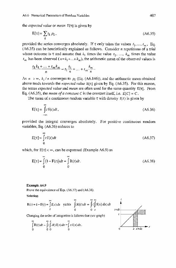
A6.6 Numerical Parameters of Random Variables 407
ihe expected value or mean E[T] is given by
E [ T I = ~ ~ ~ P ~ , (A6.35) k
provided the series converges absolutely. If z only takes the values t l , . . ., tm , Eq. (A6.35) can be heuristically explained as follows. Consider n repetitions of a trial whose outcome is z and assume that kl times the value tl , . . . , km times the value tm has been observed ( n = kl +... + km) , the ariihmetic mean of the observed values is
As n + W, ki l n converges to pi (Eq. (A6.146)), and the arithmetic mean obtained above tends towards the expected value E[z] given by Eq. (A6.35). For this reason, the terms expected value and mean are often used for the same quantity E[z]. From Eq. (A6.35), the mean of a constant Cis the constant itself, i.e. E[C] = C.
The mean of a continuous random variable z with density f ( t ) is given by
provided the integral converges absolutely. For positive continuous random variables, Eq. (A6.36) reduces to
E[z] = J t f ( t ) dt 0
which, for E[d < W , can be expressed (Example A6.9) as
Example A6.9 Prove the equivalence of Eqs. (A6.37) and (A6.38).
Solution e3 m m m t
R ) = 1 F ) = ( X ) yields I ~ ( t ) d t = I ( j f ( x ) d i ) d t t 0 0 t
Changing the order of integration it follows that (see graph)
m 00 X m
j ~ ( t ) d t = I(jdt)f(x)dx =Ixf(x)dx. 0 0 0 0
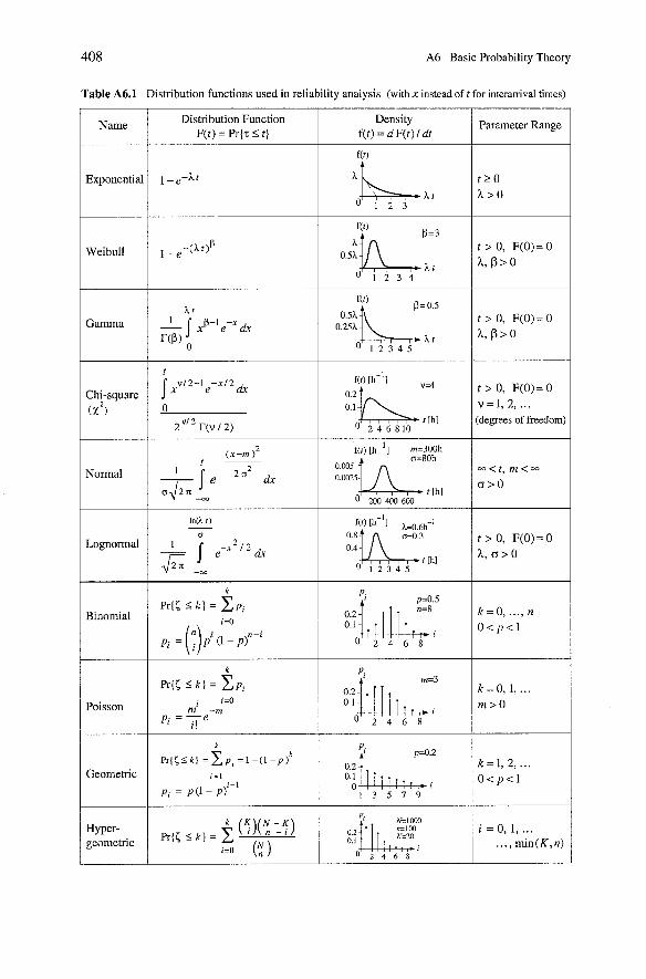
408 A6 Basic Probability Theory
Table A6.1 Distribution functions used in reliability analysis (with X instead of t for interamval times)
Name Distribution Function F(t) = Pr{z I t ]
Density Parameter Range f(t) = d F(t) l dt
Exponential
Weibull
Gamma
f(0 t > 0, F(O)=O v = l , 2, ...
+ 2 [hl (degrees of freedom:
(x-m )' t
2 a2 dx Normal
Lognormal
Binomial
Poisson
k
P r ( < < k ] =Epi =l-(l-p)k
i = l i-l
Pi = P U - P ) Geometric
Hyper- geometric
k K N - K Pr[< < k l = ( i N n - i )
i=o (n )
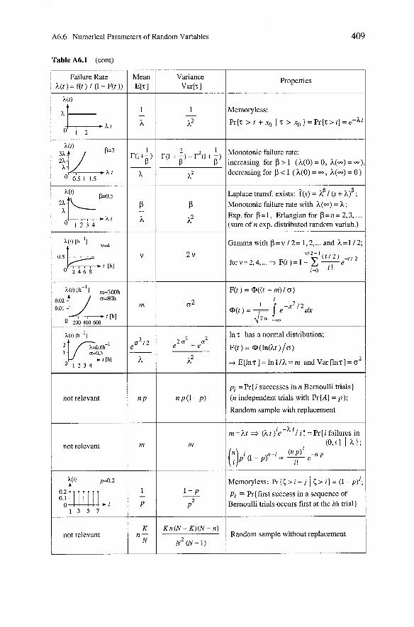
A6.6 Numencal Parameters of Random Variables
Table A6.1 (cont)
Mean E h 1
Properties Failure Rate h(t ) = f(t ) 1 (1 - F(t ))
Memoryless:
Pr{z > t +xo 1 z > xo] = P r { ~ > t ] = e - ~
Monotonic failure rate: increasing for ß > 1 (h(0) = 0, L(=) = = decreasing for ß 1 ( h(0) = m , L(-) = 0:
Laplace transf. exists: T ( s ) = hß I (s + h)' ; Monotonic failure rate with h(-) = h ; Exp. for ß = 1, Erlangian for ß = n = 2,3, . . (sum of n exp. distributed random variab.)
Gamma with ß = v 12= 1,2, ... and h = l / 2
lnz has a normal distribution;
F(t) = @(ln(ht)/o)
pi =Pr( i successes in n Bernoulli tnals} (n independent trials with Pr{A} = p ) ;
Random sample with replacement
not relevant
not relevant
Memoryless: ~r { C > i + j 1 > i ) = (1 -
Pi = Pr{first success in a sequence of Bernoulli tnals occurs first at the ith trial]
Random sample without replacement not relevant
410 A6 Basic Probability Theory
For the expected value of the random variable q = U(T)
m
E[ril= C. u(tk ~ , k or E[q] = j u(t) f (t) dt k -m
holds, provided that series and integral converge absolutely. Two particular cases of Eq. (A6.39) are:
1. u(x) = Cx,
2. u(x) = xk, which leads to the k th moment of T,
Further important properties of the mean are given by Eqs. (A6.68) and (A6.69).
A6.6.2 Variance
The variance of a random variable z is a measure of the spread (or dispersion) of the random variable around its mean E[T]. Variance is defined as
Var[z] = E[(z - ~ [ z ] ) ~ ] , (A6.42)
and can be calculated as
for a discrete random variable. and as
01
Var[z] = ( t - E[T])~ f ( t ) dt -01
for a continuous randorn variable. In both cases,
If E[T] or Var[~] is infinite, z is said to have an infinite variance. For arbitrary constants C and A, Eqs. (A6.45) and (A6.40) yield
Var[Cz - A] = C2 Var[z]
and
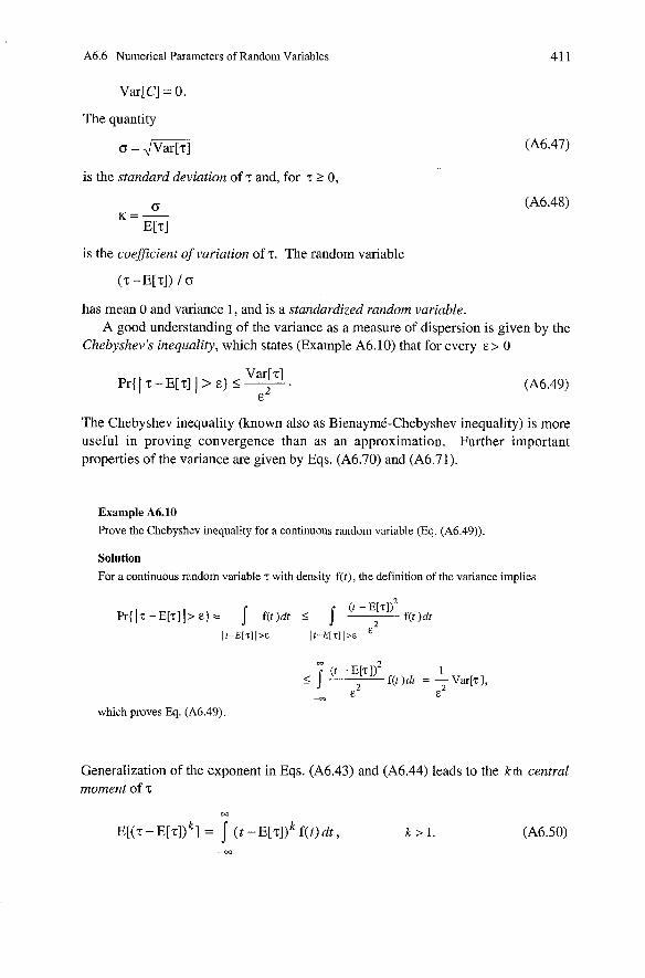
A6.6 Numerical Parameters of Random Variables
Var[C] = 0.
The quantity
o=.\ivar[zl
is the standard deviation of T and, for t 2 0,
is the coeficient of variation of T. The random variable
(T -E[T]) / o
has mean 0 and variance 1, and is a standardized random variable. A good understanding of the variance as a measure of dispersion is given by the
Chebyshev's inequality, which states (Example A6.10) that for every E > 0
The Chebyshev inequality (known also as Bienaym6-Chebyshev inequality) is more useful in proving convergence than as an approximation. Further important properties of the variance are given by Eqs. (A6.70) and (A6.71).
Example A6.10
Prove the Chebyshev inequality for a continuous random variable (Eq. (A6.49)).
Solution For a continuous random variable T with density f(t), the definition of the variance implies
which proves Eq. (A6.49).
Generalization of the exponent in Eqs. (A6.43) and (A6.44) leads to the kth central moment of T
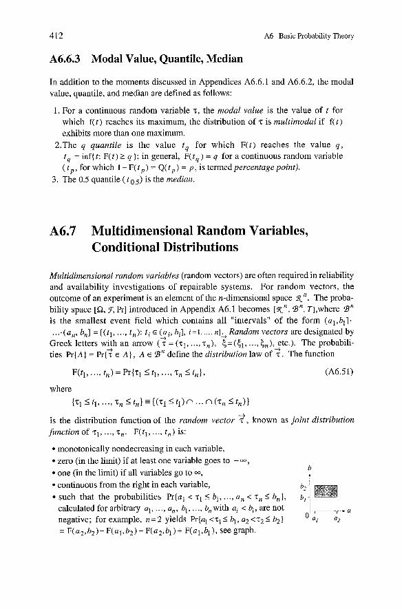
412 A6 Basic Probability Theory
A6.6.3 Modal Value, Quantile, Median
In addition to the moments discussed in Appendices A6.6.1 and A6.6.2, the modal value, quantile, and median are defined as follows:
1 . For a continuous random variable T , the modal value is the value o f t for which f ( t ) reaches its maximum, the distribution o f z is multimodal i f f ( t ) exhibits more than one maximum.
2.The q quantile is the value tq for which F(t) reaches the value q ,
tq = infit: F(t) 2 q J ; in general, F(t, ) = q for a continuous random variable ( t,, for which 1 - F(tp) = Q( tp ) = P , is termed percentage point).
3. The 0.5 quantile ( t 0 ,5 ) is the median.
A6.7 Multidimensional Random Variables, Conditional Distributions
Multidimensional random variables (random vectors) are often required in reliability and availability investigations o f repairable Systems. For random vectors, the outcome of an experiment is an element o f the n-dimensional space %-,. The proba- bility space [Q, F, Pr] introduced in Appendix A6.1 becomes [R, , Bn, T],where B" is the smallest event field which contains all "intervals" o f the form (al ,bl] . ....( a„ b,] = ( ( t l , .. ., t , ) : t i E (ai, bi], i =l , ... , nJi Random vectors are designated by
Greek letters with an arrow ( T = ( z l , ..., T, ) , E,= (t1, ..., E,,),:tc.). The probabili- ties Pr{A] = ~ r ( < C A} , A E Bn define the distribution law o f T . The function
F(tl, . . . , t,) = P ~ { T ~ 5 tl , . . . , T , 5 t,} , (A6.51)
where {zl 5 tl, . . ., zn I t,) = { (z l 5 t l ) n . .. n ( T , 5 t,)}
-+ is the distribution function o f the random vector T , known as joint distribution jünction of z l , . . . , T,. F(tl, . . . , t,) is:
monotonically nondecreasing in each variable, Zero (in the limit) i f at least one variable goes to - W ,
one (in the limit) i f all variables go to W, b
continuous from the right in each variable, such that the probabilities Pr{al < zl 4 bl, ..., an < T , I b,}, calculated for arbitrary al, .. ., a„ bl, . . ., b, with ai < bi, are not negative; for example, n= 2 yields Pr{al <T, I bl, a2 <z2 4 b2) = F(a2,bz)-F(al,b2)- F(a2,bl)+ F(al,bl), see graph.
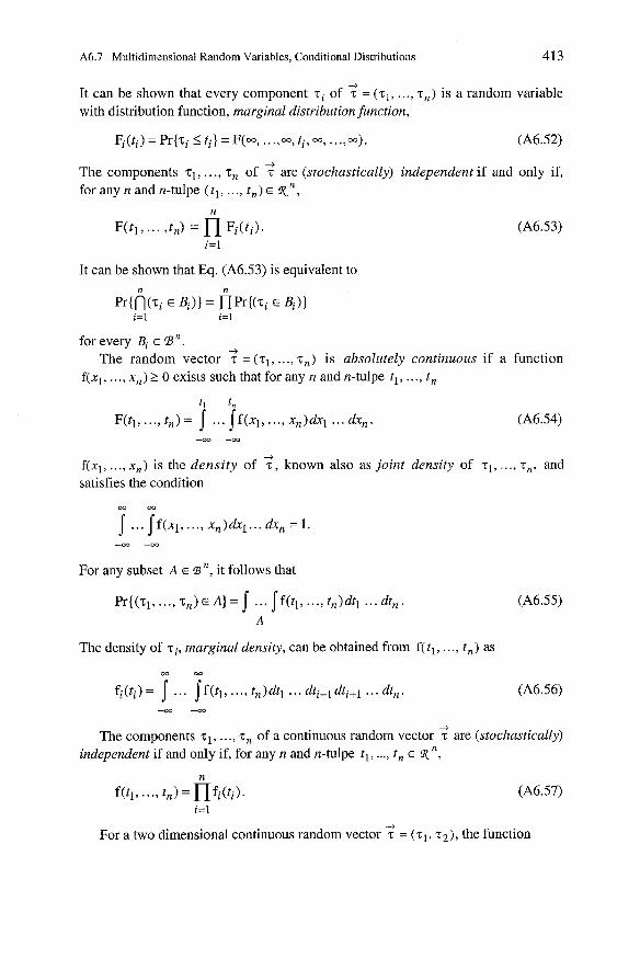
A6.7 Multidimensional Random Variables. Conditional Distributions 413
-+ It can be shown that every component zi of z = (zl , ..., T,) is a random variable with distribution function, marginal distribution function,
Fi(ti) = P ~ { T ~ 5 ti} = F(w, ...,M, ti, 00, . . .,00). (A6.52)
The components 71, . . ., 7, of -2 are (stochastically) independent if and only if, for any n and n-tulpe ( tl, . . . , t,) E R,,
n
F ( ~ ~ , ... J,) = n F ~ ( ~ ~ ) . (A6.53) i=l
It can be shown that Eq. (A6.53) is equivalent to
for every Bi E 2? n. -+
The random vector z = (T„ ..., T,) is absolutely continuous if a function f(xl, . . ., X,) 2 0 exists such that for any n and n-tulpe tl, . . ., t,
-+ f(xl, ..., X,) is the density of T , known also as joint density of zl, ..., T,. and satisfies the condition
For any subset A E B n, it follows that
The density of zi, marginal densiq, can be obtained from f(tl, ..., t,) as
+ The components TI, . . ., 7, of a continuous random vector z are (stochastically)
independent if and only if, for any n and n-tulpe tl, ..., t, E Rn,
-+ For a two dimensional continuous random vector z = (zl , z2), the function
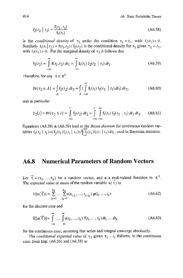
A6 Basic Probability Theory
is the conditional density
(A6.58)
of under the condition zl = t l , with f l ( t l ) > 0 . Similarly f l( t l I t 2 ) = f ( t l , t2 ) l f2 ( t2 ) is the conditional density for zl given z2 = t2 , with f2 ( t2 ) > 0. For the marginal density of . L ~ it follows that
Therefore, for any A E B'
and in particular
Equations (A6.58) & (A6.59) lead to the Bayes theorem for continuous random var- t-
iable ( t 1 t ) ( ( t f 1 t )) I f 2 ( t 2 ) f ( t 1 t 2 ) dt2, used in Bayesian statistics. -
A6.8 Numerical Parameters of Random Vectors
4 Let T = ( T ~ , ..., T, ) be a random vector, and U a real-valued function in R,.
-3 The expected value or mean of the random variable U( T ) is
for the discrete case and
for the continuous case, assuming that series and integral converge absolutely. The conditional expected value of T Z given = tl follows, in the continuous
case, from Eqs. (A6.36) and (A6.58) as
A6.8 Numerical Parameters of Random Vectors
Thus the unconditional expected value of can be obtained from
Equation (A6.65) is known as the formula of total expectation and is useful in practical applications.
A6.8.1 Covariance Matrix, Correlation Coefficient
+ Assuming for T = ( T ~ , . . . , T,) that Var [TJ < m , i = 1 , . . . , n, an important rough characterization of a random vector is the covariance matrix I a , 1, where
a = COV[T. 't .] = E[('ti - E[zi])(zj - E['tj])] V 1' J
are given in the continuous case by
The diagonal elements of the covariance matrix are the variances of components zi, i = 1, ..., n. Elements outside the diagonal give a measure of the degree of dependency between components (obviously a , = a ji). For zi independent of T j ,
U . . = a .. = 0 holds. iJ 1 2 + For a two dimensional random vector z = ( T ~ , T ~ ) , the quantity
is the correlation coefflcient of the random variables z1 and TZ, provided
oi = l/var[zi] < 00, i = 1, 2.
The main properties of the correlation coefficient are:
1. I p l I l .
2. if zl and z2 are independent, then p = 0.
3. p = I1 if and only if zl and are linearly dependent.
416 A6 Basic Probability Theory
A6.8.2 Further Properties of Expected Value and Variance
-+ Let TI, . . ., T, be arbitrary random variables (components of a random vector T ) having finite variances and Cl, ..., C, constants. From Eqs. (A6.62) or (A6.63) and (A6.40) it follows that
E[CIzl + ... +C,T,]= C1E[~,]+ ... +C,E[z,]. (A6.68)
If T, and are independent then, fromEq. (A6.63) and Eq. (A6.45),
E[zl Z ~ I = E [ T ~ I E [ T ~ ] and Var[T1 z2] =E[zf] E[T$] - ~ ~ [ z ~ ] ~ ~ [ z ~ ] . (A6.69)
The variance of a sum of independent random variables zl, ..., T, is obtained from Eqs. (A6.62) or (A6.63) and (A6.69) as
For a sum of arbitrary random variables TI , . ..,T„ the variance can be obtained for i, j E (1, ..., n ]
A6.9 Distribution of the Sum of Independent Positive Random Variables and of T„, T„,
Let .zl and be independent non-negative arithmetic random variables with ai = Pr{Tl = i ) , bi = = i ) , i = 0,1, .... Obviously, zl +T2 is also arithmetic, and therefore
The sequence CO, CI, ... is the convolution of the sequences ao, a l , ... and bo, bl, .... Now, let zl and z2 be two independent positive continuous random variables
with distribution functions Fl(t), F2(t) and densities fl(t), f2(t), respectively (F1(0) = F2(0) = 0). Using Eq. (A6.55), it can be shown (Example A6.11 and Fig. A6.4) that for the distribution of = zl + z2
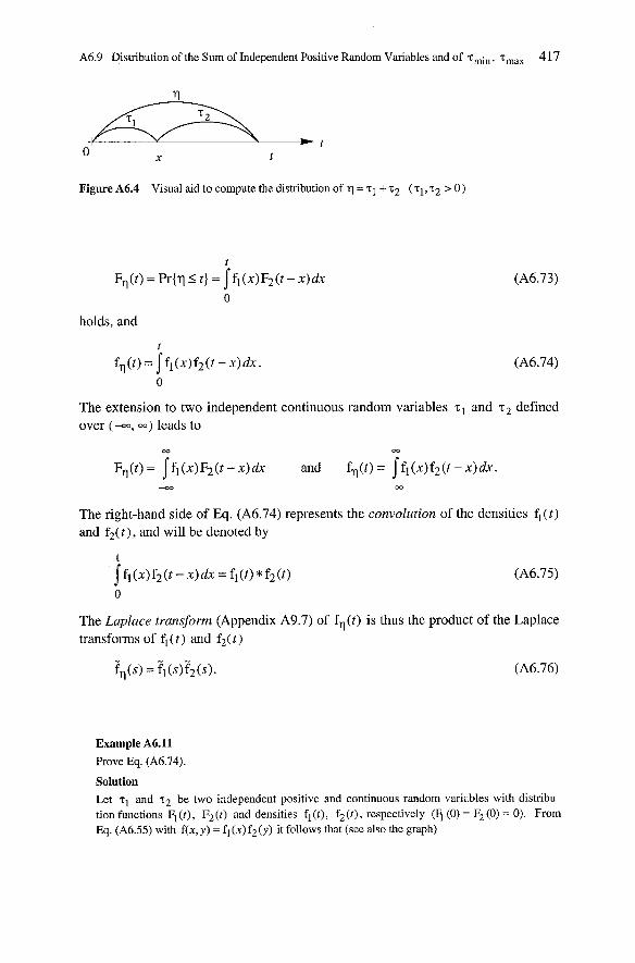
A6.9 Distribution of the Sum of Independent Positive Random Variables and of zmi„ T„, 417
Figure A6.4 Visual aid to compute the distnbution of T = TI + TZ (TI, 22 > 0 )
holds, and
The extension to two independent continuous random variables and z2 defined over (-=, =) leads to
The right-hand side of Eq. (A6.74) represents the convolution of the densities f l ( t )
and f2(t) , and will be denoted by
The Laplace transform (Appendix A9.7) of fq(t) is thus the product of the Laplace transforms of f l ( t ) and f2( t )
Sq (s) = S1 (s) S2 (8).
Example A6.11
F'rove Eq. (A6.74).
Solution Let '1 and 72 be two independent positive and continuous random variables with distribu- tion functions Fl (t), F2(t) and densities fl (t), f2 ( t ) , respectively (F; (0) = F2 (0) = 0). From Eq. (A6.55) with f(x, y) = fl(x)f2(y) it follows that (see also the graph)
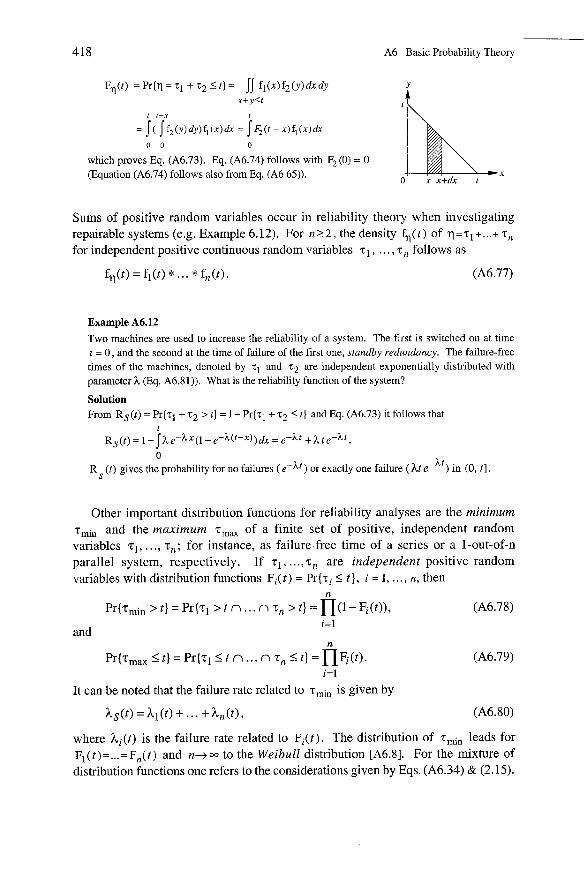
418 A6 Basic Probability Theory
F 11 ( t ) = P r { r = q + ~ ~ - < t ) = ~ ~ f i ( x ) f 2 ( y ) d x d y Y
x+y<t t
I 1 - X f
= J ( Jf,(y)dy)f,(x)& = j$(f - ~ ) f , ( x ) & 0 0 0
which proves Eq. (A6.73). Eq. (A6.74) follows with F2 (0) = 0 (Equation (A6.74) follows also from Eq. (A6.65)). X
0 x X+& t
Sums of positive random variables occur in reliability theory when investigating repairable Systems (e.g. Example 6.12). For n r 2 , the density f q ( t ) of q =TI +...+ T,
for independent positive continuous random variables T I , . . . , T, follows as
fr(t)=fi(t)* ... *fn(t). (A6.77)
Example A6.12 Two machines are used to increase the reliability of a system. The first is switched on at time t = 0 , and the second at the time of failure of the first one, standby redundancy. The failure-free times of the machines, denoted by TI and 22 are independent exponentially distributed with Parameter ?L (Eq. A6.81)). What is the reliability function of the system?
Solution From RS(t) = P ~ { T ~ + ' 2 > t] = 1 - Pr{zl + 22 < t} and Eq. (A6.73) it follows that
0 R (t) gives the probability for no failures ( e-ht) or exactly one failure ( ht e-") in (0, t].
Other important distribution functions for reliability analyses are the minimum e„ and the maximum T„, of a finite set of positive, independent random variables TI, . . ., T,; for instance, as failure-free time of a series or a 1-out-of-n parallel system, respectively. If T I , . . ., T , are independent positive random variables with distribution functions Fi(t) = P ~ { T ~ I t ] , i = 1 , ... , n, then
n Pr{zmin > t } = P ~ { T ~ > t n ... n T, > t } = n < 1 - ~ ~ ( t ) ) , (A6.78)
i=l and
i=l It can be noted that the failure rate related to T,~, is given by
where hi(t) is the failure rate related to Fi(t) . The distribution of T „ leads for F I ( t )= ...= Fn(t) and n+.o to the Weibull distribution [A6.8]. For the mixture of distribution functions one refers to the considerations given by Eqs. (A6.34) & (2.15).
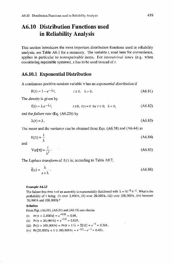
A6.10 Distribution Functions used in Reliability Analysis
A6.10 Distribution Functions used in Reliability Analysis
This section introduces the most important distribution functions used in reliability analysis, See Table A6.1 for a Summary. The variable t, used here for convenience, applies in particular to nonrepairable items. For interarrival times (e.g. when considering repairable systems), x has to be used instead oft .
A6.10.1 Exponential Distribution
A continuous positive random variable z has an exponential distribution if
The density is given by
f(t) = he-At, t 20, f(t)= o for t < O; h > 0, (A6.82)
and the failure rate (Eq. (A6.25)) by
h(t) = h . (A6.83)
The mean and the variance can be obtained from Eqs. (A6.38) and (A6.44) as
1 E[T] = -
h and
The Laplace transform of f(t) is, according to Table A9.7,
Example A6.13 The fahre-free time T of an assembly is exponentially distributed with h = 1oM5 h-l. What is the probability of T being (i) over 2,000 h, (ii) over 20,000 h, (iii) over 100,000 h , (iv) between 20,000 h and 100,000 h ?
Solution From Eqs. (A6.81), (A6.24) and (A6.19) one obtains
(i) Pr{z > 2,000h) = eT0'02 = 0.98,
(ii) Pr{z > 20,000h) = e-0'2 = 0.819, (iii) Pr{% > 100,000 h} = Pr(7 > l lh = E[z]} = e-' = 0.368,
(iv) Pr(20,OOOh < T 1 100,000h) = e-0.2 - e-I = 0.451.
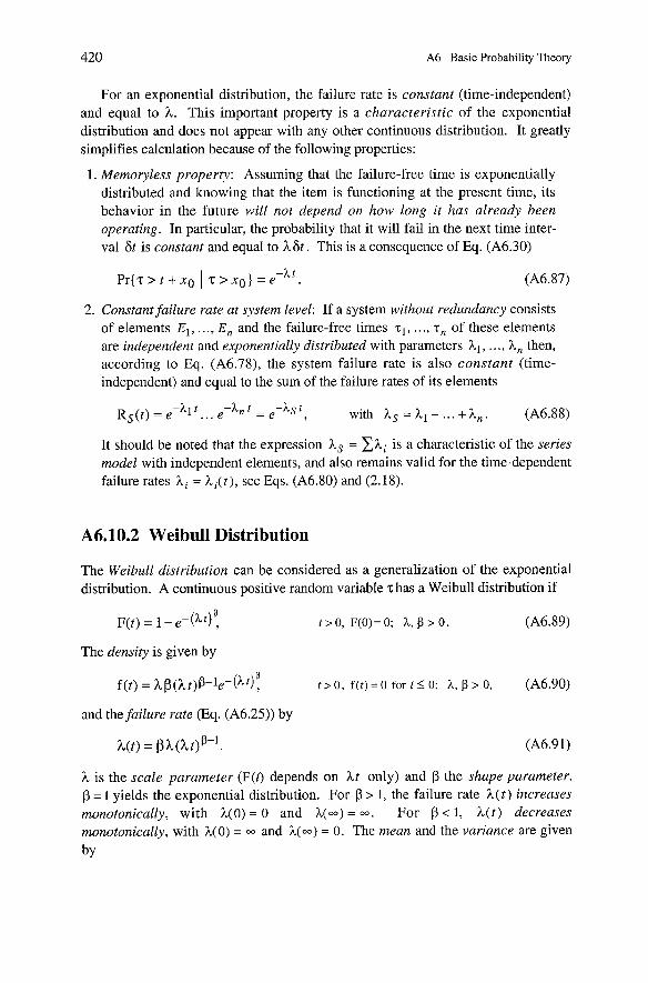
420 A6 Basic Probability Theory
For an exponential distribution, the failure rate is constant (time-independent) and equal to h. This important property is a characteristic of the exponential distribution and does not appear with any other continuous distribution. It greatly simplifies calculation because of the following properties:
1. Memoryless property: Assuming that the failure-free time is exponentially distributed and knowing that the item is functioning at the present time, its behavior in the future will not depend on how long it has already been operating. In particular, the probability that it will fail in the next time inter- val 6t is constant and equal to h & . This is a consequence of Eq. (A6.30)
2. Constant failure rate at system level: If a system without redundancy consists of elements EI, ..., E , and the failure-free times T ~ , ..., T, of these elements are independent and exponentially distributed with Parameters A l , . . ., X , then, according to Eq. (A6.78), the system failure rate is also constant (time- independent) and equal to the sum of the failure rates of its elements
~ ~ ( t ) = = e - h ~ , with hs = AI + . . . +L, . (A6.88)
It should be noted that the expression hs = E h i is a characteristic of the series model with independent elements, and also remains valid for the time-dependent failure rates Ai = hi( t j , see Eqs. (A6.80) and (2.18).
A6.10.2 Weibull Distribution
The Weibull distribution can be considered as a generalization of the exponential distribution. A continuous positive random variable T has a Weibull distribution if
The density is given by
and the failure rate (Eq. (A6.25)) by
h is the scale Parameter ( F @ ) depends on At only) and ß the shape parameter. ß = 1 yields the exponential distribution. For ß > 1, the failure rate h ( t ) increases monotonically, with h(Oj = 0 and ?L(-) = - . For ß < 1, ?L( t j decreases monotonically, with h(0) = and ?L(-) = 0 . The mean and the variance are given
by
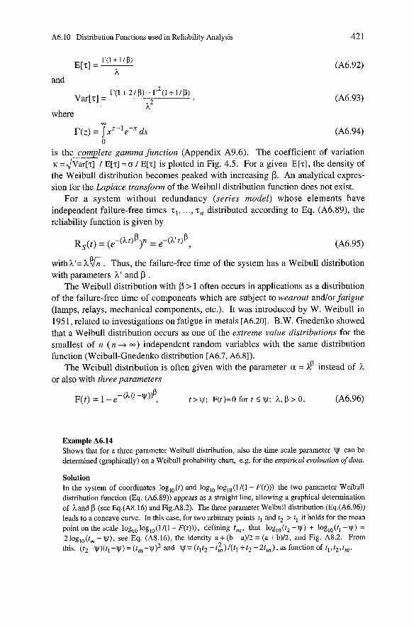
A6.10 Distribution Functions used in Reliability Analysis 42 1
h and
where C o
r(s) = Jxz-le-x dx 0
is the complete gamma function (Appendix A9.6). The coefficient of variation K = J ~ I E[T] =a I E[%] is plotted in Fig. 4.5. For a given E[T], the density of the Weibull distribution becomes peaked with increasing P. An analytical expres- sion for the Laplace transform of the Weibull distribution function does not exist.
For a system without redundancy (series model) whose elements have independent failure-free times TI, . . ., T, distributed according to Eq. (A6.89), the reliability function is given by
with?LV= ?L!&. Thus, the failure-free time of the system has a Weibull distribution with Parameters h' and ß .
The Weibull distribution with ß > 1 often occurs in applications as a distribution of the failure-free time of components which are subject to wearout andlor fatigue (lamps, relays, mechanical components, etc.). It was introduced by W. Weibull in 1951, related to investigations on fatigue in metals [A6.20]. B.W. Gnedenko showed that a Weibull distribution occurs as one of the extreme value distributions for the smallest of n ( n + W ) independent random variables with the same distribution function (Weibull-Gnedenko distribution [A6.7, A6.81).
The Weibull distribution is often given with the parameter a = ?Lß instead of ?L or also with three Parameters
Example A6.14 Shows that for a three parameter Weibull distribution, also the time scale Parameter can be determined (graphically) on a Weibull probability chart, e.g. for the empincal evaluation of data.
Solution In the system of coordinates log„(t) and loglo log„(ll(l- F(t))) the two parameter Weibull distribution function (Eq. (A6.89)) appears as a straight line, allowing a graphical determination of hand ß (see Eq.(A8.16) and Fig.Ag.2). The three parameter Weibull distribution (Eq.(A6.96)) leads to a concave curve. In this case, for two arbitrary points tl and t2 > t, it holds for the mean point on the scale loglo 10g,~(l 41- F(t))), defining t„ that loglo(t2 -W) + loglo(tl -Y) = 210glo(t, - Y), see Eq. (A8.16), the identity a + (b - a)/2 = (a + b)/2, and Fig. A8.2. From this, (t2 -y)(tl -W) = ( t , - ~ ) ~ and = (tlt2 -&) l ( t l + t2 - 2 t m ) , as function of tl, t2, tm.
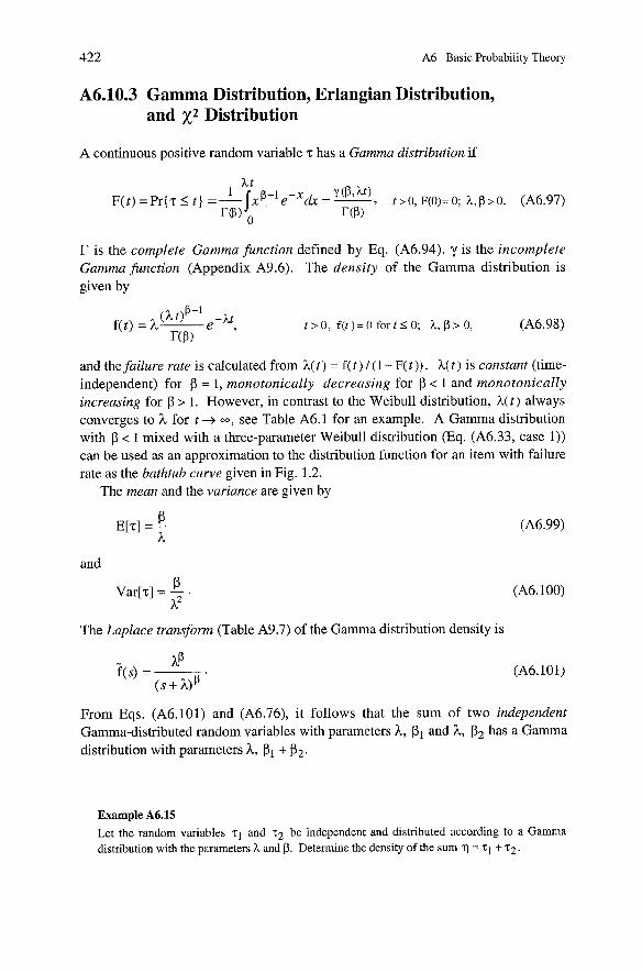
422 A6 Basic Probability Theory
A6.10.3 Gamma Distribution, Erlangian Distribution, and ~2 Distribution
A continuous positive random variable T has a Gamma distribution if
r is the complete Gamma function defined by Eq. (A6.94). y is the incomplete Gamma function (Appendix A9.6). The density of the Gamma distribution is given by
and the failure rate is calculated from h ( t ) = f ( t ) l ( 1 - F(t)) . h ( t ) is constant (time- independent) for ß = 1, rnonotonically decreasing for ß < 1 and monotonically increasing for ß > 1. However, in contrast to the Weibull distribution, h( t ) always converges to ?L for t + W , see Table A6.1 for an example. A Gamma distribution with ß < 1 mixed with a three-parameter Weibull distribution (Eq. (A6.33, case 1)) can be used as an approximation to the distribution function for an item with failure rate as the bathtub cuwe given in Fig. 1.2.
The mean and the variance are given by
and
The Laplace transform (Table A9.7) of the Gamma distribution density is
From Eqs. (A6.101) and (A6.76), it follows that the sum of two independent Gamma-distributed random variables with parameters h, ß1 and h, ß2 has a Gamma distribution with parameters h, ß1 + ß2.
Example A6.15 Let the random variables zl and 22 be independent and distributed according to a Gamma distnbution with the parameters h and ß. Determine the density of the sum q = 'CI + 22.
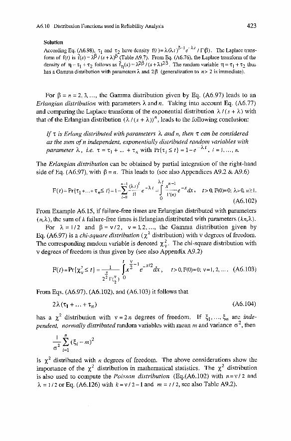
A6.10 Distribution Functions used in Reliability Analysis 423
Solution According Eq. (A6.98), 71 and 72 have density f(t )= h (h t / r@). The Laplace trans- form of f(t) is f(s) = ?@ / ( s + h ) ß (Table A9.7). From Eq. (A6.76), the Laplace transform of the density of q = zl + 72 follows as fr(s) = x2ß / (s + ~ ) ~ ß . The random variable q = 71 + 72 thus has a Gamma distribution with parameters h and 2ß (generalization to n> 2 is immediate).
For ß = n = 2,3 , ..., the Gamma distribution given by Eq. (A6.97) leads to an Erlangian distribution with parameters h and n. Taking into account Eq. (A6.77) and comparing the Laplace transform of the exponential distribution h I (s + h ) with that of the Erlangian distribution ( h I ( s + L)),, leads to the following conclusion:
If z is Erlang distributed with parameters ?L und n, then T can be considered as the sum of n independent, exponentially distributed random variables with Parameter h , i.e. T = z l + ... +T, with P r ( z i < t } = 1 - e C a t , i =1, ..., n.
The Erlangian distribution can be obtained by partial integration of the right-hand side of Eq. (A6.97), with ß = n. This leads to (see also Appendices A9.2 & A9.6)
From Example A6.15, if failure-free times are Erlangian distributed with parameters (n, L), the sum of k failure-free times is Erlangian distributed with parameters (kn, h).
For h = 1 1 2 and ß = V 1 2 , V = i, 2, . .., the Gamma distribution given by Eq. (A6.97) is a chi-square distribution (x2 distribution) with V degrees of freedom. The corresponding random variable is denoted X t. The chi-square distribution with V degrees of freedom is thus given by (see also Appendix A9.2)
t Ll -X12 - I x 2 e dx, r>o.p(o)=o;v=l.2 ,.... (A6.103) ~ ( t ) = ~ r { ~ t 5 t ] = ,-
22r(:) 0
From Eqs. (A6.97), (A6.102), and (A6.103) it follows that
has a distribution with V = 2 n degrees of freedom. If Cl, ..., 5, are inde- pendent, normally distributed random variables with mean m and variance 02, then
is distributed with n degrees of freedom. The above considerations show the importance of the distribution in mathematical statistics. The distribution is also used to compute the Poisson distribution (Eq.(A6.102) with n = v 1 2 and h = 112 or Eq. (A6.126) with k = v / 2 - 1 and m = t / 2, See also Table A9.2).
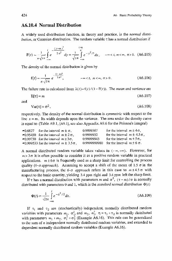
424 A6 Basic Probability Theory
A6.10.4 Normal Distribution
A widely used distribution function, in theory and practice, is the normal distri- bution, or Gaussian distribution. The random variable T has a normal distribution if
The density of the normal distribution is given by
The failure rate is calculated from A ( t ) = f ( t ) l (1 - F(t)). The mean and variance are
E[T] = m and
Var[z] = 0 2 ,
respectively. The density of the normal distribution is symmetric with respect to the line X = m . Its width depends upon the variance. The area under the density curve is equal to (Table A9.1, [A9.1], See also Appendix A9.6 for the Poisson's integral)
0.6827 for the interval rn f o, 0.9999367 for the interval rn + 4 o, 0.95450 for the interval m f 2 o, 0.9999932 for the interval rn + 4.5 o , 0.99730 for the interval rn f 3 G, 0.99999943 for the interval rn f 5 0,. 0.999533 for the interval rn I 3.5 o , 0.9999999980 for the interval rn + 6 o.
A normal distributed random variable takes values in ( -W, +W). However, for m > 3 o it is often possible to consider it as a positive random variable in practical applications. rn + 6 o is frequently used as a sharp limit for controlling the process quality (6-oapproach). Assuming to accept a shift of the mean of 1.5 o in the manufacturing process, the 6-0 approach refers in this case to rn 14.5 o with respect to the basic quantity, yielding 3.4 ppm right and 3.4 ppm left the sharp lirnit.
2 If T has a normal distribution with parameters m and o , ( T - rn) 1 o is normally distributed with parameters 0 and 1, which is the standard normal distribution @ ( t )
If and z2 are (stochastically) independent, normally distributed random variables with parameters rn l , o:, and rn2, G:, q = + 7 2 is normally distributed with parameters rnl + in2, o: + 02 (Example A6.16). This rule can be generalized to the sum of n independent normally distributed random variables, and extended to dependent normally distributed random variables (Example A6.16).
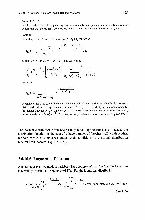
A6.10 Distribution Functions used in Reliability Analysis
Example A6.16 Let the random variables 71 and 9 be (stochastically) independent and normally distributed with means ml and m2 and variances o; and o;. Give the density of the sum q = . L ~ + T ~ .
Solution According to Eq. (A6.74), the density of q = 71 + T ~ ~ O ~ ~ O W S as
Setting u = n - m l , V = t - ml - m 2 , and considering
the result
is obtained. Thus the sum of independent normally distributed random variables is also normally 2 2 distributed with mean ml + m2 and variance o , + 0 2 . If 21 and 72 are not (stochastically)
independent, the distribution function of zl + 72 is still a normal distribution with m = ml + m2, 2 2 2 but with variance o = o, + o2 + 2p ol 0 2 , where p is the correlation coefficient (Eq. (A6.67)).
The normal distribution often occurs in practical applications, also because the distribution function of the sum of a large number of (stochastically) independent random variables converges under weak conditions to a normal distribution (central lirnit theorem, Eq. (A6.148)).
A6.10.5 Lognormal Distribution
A continuous positive random variable T has a lognormal distribution if its logarithm is normally distributed (Example A6.17). For the lognormal distribution,
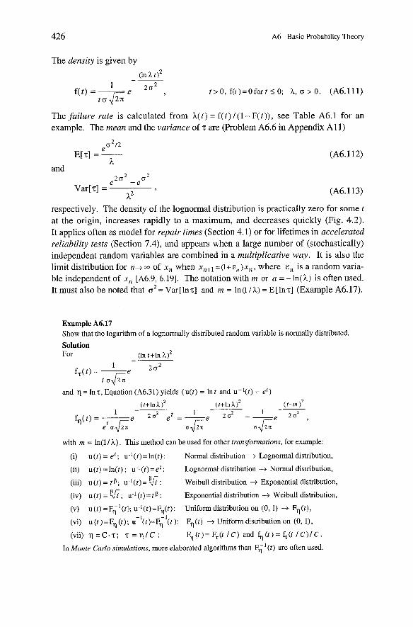
A6 Basic Probability Theory
The density is given by
(in L t )2 -- 1
f(t) = - 2 0 2 t>O, f ( t )=Ofor t<O; h, 0 > 0 . (A6.111) t 0 6
The failure rate is calculated from A(t) = f ( t ) / ( l - F(t)), see Table A6.1 for an example. The mean and the variance of T are (Problem A6.6 in Appendix A l 1)
e 0 2 / 2
E[T] = - a and
respectively. The density of the lognormal distribution is practically Zero for some t at the origin, increases rapidly to a maximum, and decreases quickly (Fig. 4.2). It applies often as model for repair times (Section 4.1) or for lifetimes in accelerated reliability tests (Section 7.4), and appears when a large number of (stochastically) independent random variables are combined in a multiplicative way. It is also the limit distribution for n+ of X, when x , + ~ = (1 + E, )X,, where E, is a random varia- ble independent of X, [A6.9, 6.191. The notation with rn or a = - h ( h ) is often used. It must also be noted that 0' = Var [lnz] and rn = In (1 / h) = E [ l n ~ ] (Example A6.17).
Example A6.17 Show that the logarithm of a lognomally distributed random variable is normally distributed.
Solution For (ln t+ln h)'
1 fT( t ) = - 2 0 2
and q = lnz, Equation (A6.31) yields (u(t) = lnt and U-'(t) = et)
with m = ln(1 I L). This method can be used for other transformations. for exarnple:
(i) U (t) = et ; U-' (t) = ln(t) : Normal distribution 4 Lognormal distribution,
(ii) u(t) = ln(t) ; U-'(2) =er : Lognormal distribution -t Normal distribution,
(iii) U (t) = t ß; U-' (t) = : Weibull distribution + Exponential distribution,
(iv) U (t) = V ; U-I (t) = t ß : Exponential distribution -t Weibull distribution,
(V) U (t) =F; ' (2); U-I (t) =Fq(t) : Uniform distribution on (0, 1) -+ F? (t),
(vi) U (t )=Fq (t); Ü 1 ( t ) = ~ i l ( t ) : F?(t) -+ Uniform distribution on (0, I),
(vii) q =C.T; z = q l C : F,(t)=F,(t / C ) and $ ( t ) = G(t l C ) / C .
In Monte Carlo simulations, more elaborated algorithms than F i l ( t ) are often used.
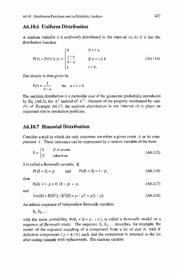
A6.10 Distribution Functions used in Reliability Analysis 427
A6.10.6 Uniform Distribution
A random variable T is uniformly distributed in the interval ( U , b) if it has the distribution function
The density is then given by
f ( t ) = --L for a < t < b . b - a
The uniform distribution is a particular case of the geometric probability introduced by Eq. (A6.3), for x1 instead of x2. Because of the property mentioned by case (V) of Example A6.17, the uniform distribution in the interval (0,l) plays an important role in simulation problems.
A6.10.7 Binomial Distribution
Consider a trial in which the only outcomes are either a given event A or its com- plement Ä. These outcomes can be represented by a randorn variable of the form
1 if A occurs 6 = {
0 othenvise.
6 is called a Bernoulli variable. If
P r{6=1}=p and P r { 6 = 0 ) = 1 - p ,
and Var[G] = ~ [ 6 2 ] - ~ 2 [ 6 ] = p - p2 = p ( l - P ) .
An infinite sequence of independent Bernoulli variables
with the same probability Pr{6i = 1) = P , i t 1, is called a Bernoulli model or a sequence of Bernoulli trials. The sequence 61, 62, . . . describes, for example, the model of the repeated sampling of a component from a lot of size N, with K defective components ( p = KIN) such that the component is retumed to the lot after testing (sample with replacement). The random variable
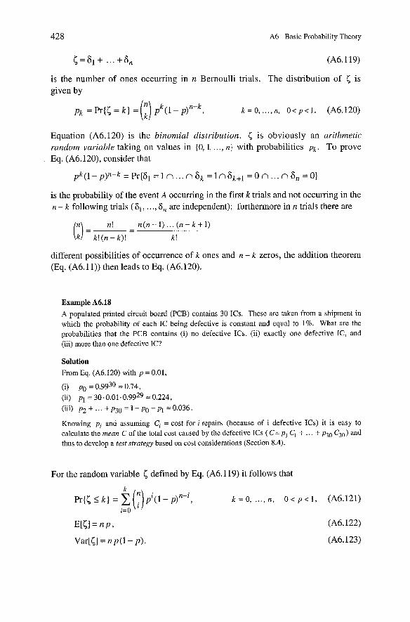
428 A6 Basic Probability Theory
is the number of ones occurring in n Bernoulli trials. The distribution of 6 is given by
Equation (A6.120) is the binomial distribution. is obviously an arithmetic random variable taking on values in ( 9 1 , . . ., n ) with probabilities pk. TO prove Eq. (A6.120), consider that
is the probability of the event A occurring in the first k trials and not occurring in the n - k following trials (SI, . . ., 6, are independent); furthermore in n trials there are
different possibilities of occurrence of k ones and n - k Zeros, the addition theorem (Eq. (A6.11)) then leads to Eq. (A6.120).
Example A6.18
A populated printed circuit board (PCB) contains 30 ICs. These are taken from a shipment in which the probability of each IC being defective is constant and equal to 1%. What are the probabilities that the PCB contains (i) no defective ICs, (ii) exactly one defective IC, and (iii) more than one defective IC?
Solution From Eq. (A6.120) with p = 0.01,
(i) po = 0 . 9 9 ~ ~ = 0.74,
(ii) p1 = 30 .0 .01 .0 .99~~ = 0.224,
(iii) p2 + . . . + p30 = 1 - po - p1 = 0.036
Knowing pi and assuming Ci = cost for i repairs (because of i defective ICs) it is easy to calculate the mean C of the total cost caused by the defective ICs (C= pl Cl + . . . + p30 C30) and thus to develop a test strategy based on cost considerations (Section 8.4).
For the random variable 5 defined by Eq. (A6.119) it follows that
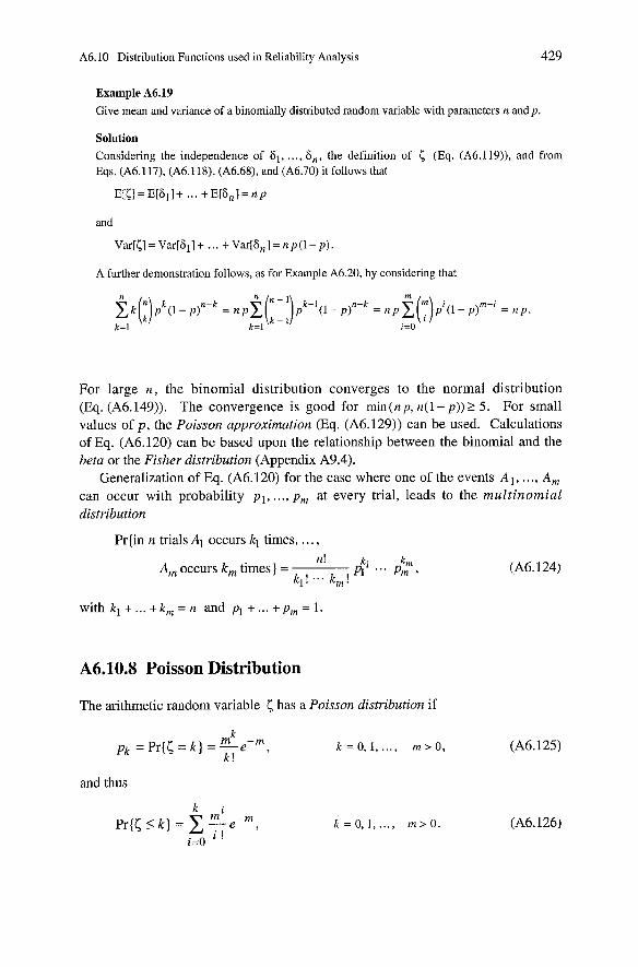
A6.10 Distribution Functions used in Reliability Analysis 429
Example A6.19 Give mean and variance of a binornially distributed random variable with Parameters n andp.
Solution Considering the independence of a l , . . . , 6„ the definition of 5 (Eq. (A6.1 lg)), and from Eqs. (A6.117), (A6.118), (A6.68), and (A6.70) it follows that
and
Var[(] = Var[S1] + . . . + Var[S,] = n p (1 - p).
A further demonstration follows, as for Example A6.20, by considering that
For large n , the binomial distribution converges to the normal distribution (Eq. (A6.149)). The convergence is good for min ( n p, n(1- p) ) 2 5 . For small values of p, the Poisson approximation (Eq. (A6.129)) can be used. Calculations of Eq. (A6.120) can be based upon the relationship between the binomial and the beta or the Fisher distribution (Appendix A9.4).
Generalization of Eq. (A6.120) for the case where one of the events A l , . . ., Am can occur with probability p l , ..., p , at every trial, leads to the multinomial distribution
Pr{in n trials Al occurs kl times, . . . , n !
Am occurs km times) = $ ... k, k,! ... k m !
with kl + ... + k m = n and pl + ... + P , = 1.
A6.10.8 Poisson Distribution
The arithmetic random variable 5 has a Poisson distribution if
k m rn p k = P r { < = k ) = - e - , k = 0 , 1 , ..., m>O, k !
and thus
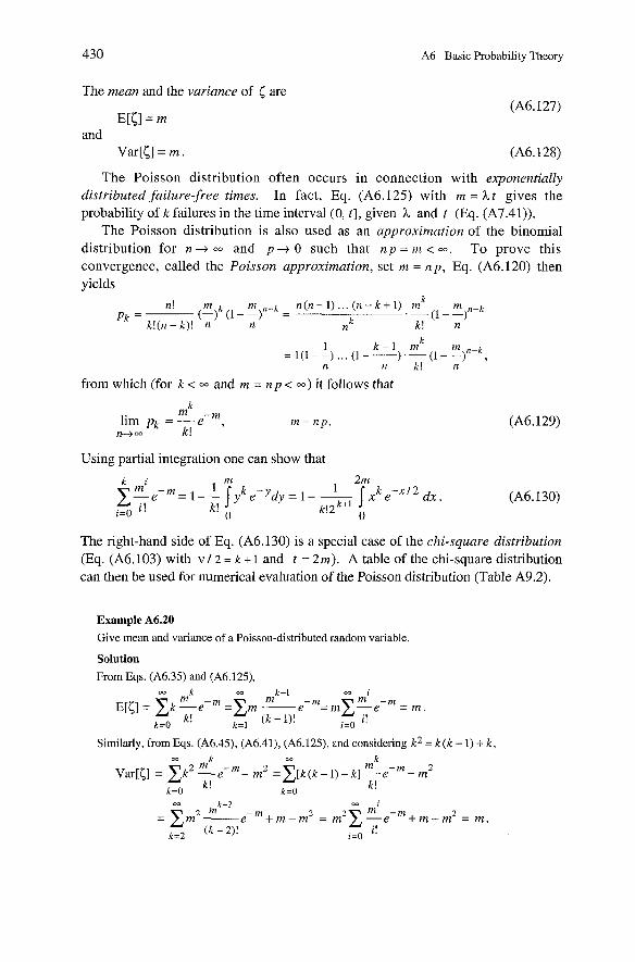
430 A6 Basic Probability Theory
The mean and the varinnce of 5 are
E[<]= m and
Var[<] = m .
The Poisson distribution often occurs in connection with exponentially distributed failure-free times. In fact, Eq. (A6.125) with m = At gives the probability of k failures in the time interval(0, t ] , given h and t (Eq. (A7.41)).
The Poisson distribution is also used as an approximation of the binomial distribution for n -+ W and p -+ 0 such that n p = m < W . To prove this convergence, called the Poisson approximation, Set m = n p , Eq. (A6.120) then yields
k n! rn k in ,,-k n(n -1 ) ... ( n - k + l ) rn rn n-k
(-1 (1--) - Pk=k!(n-k)! n k .-(1--)
k! n
1 k - 1 rn k
rn n-k = l ( 1 - - ) . . . ( 1--).-(1--) ,
n n k ! n
from which (for k < and m = n p < W ) it follows that
k m -m lim pk = -e , rn= n p .
n-S- k !
Using partial integration one can show that
The right-hand side of Eq. (A6.130) is a special case of the chi-square distribution (Eq. (A6.103) with V 1 2 = k + 1 and t = 2m). A table of the chi-square distribution can then be used for ~iumerical evaluation of the Poisson distribution (Table A9.2).
Example A6.20
Give mean and variance of a Poisson-distributed random variable.
Solution
From Eqs. (A6.35) and (A6.125),
Similarly, from Eqs. (Ah.45), (A6.41), (A6.125), and considering k2 = k ( k - 1) + k ,
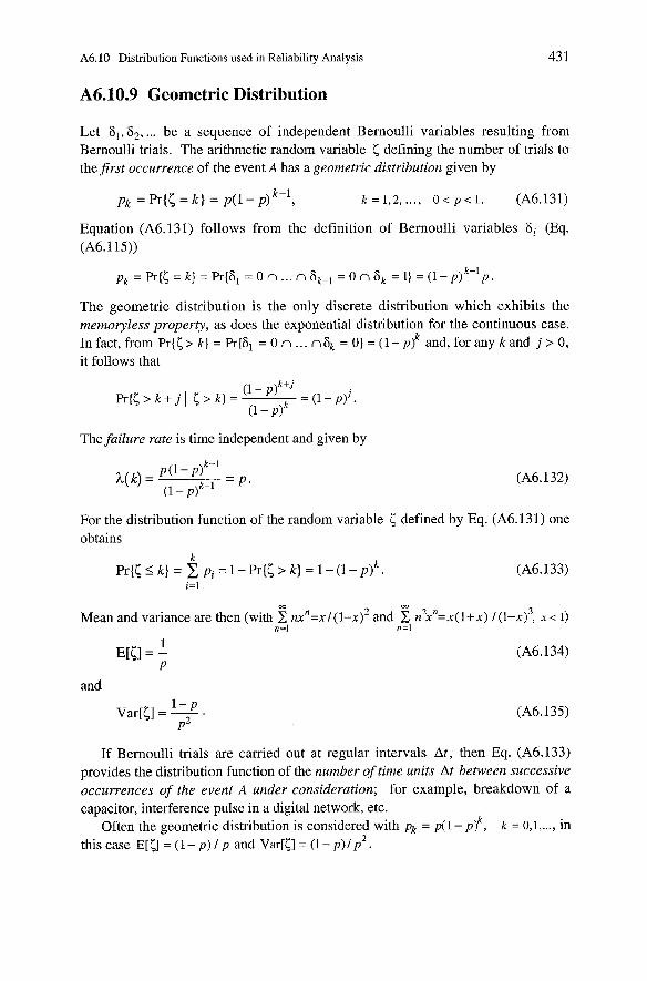
A6.10 Distribution Functions used in Reliability Analysis 43 1
A6.10.9 Geornetric Distribution
Let 81, ti2, ... be a sequence of independent Bernoulli variables resulting from Bernoulli trials. The arithmetic random variable 5 defining the number of trials to the Jirst occurrence of the event A has a geometric distribution given by
Equation (A6.131) follows from the definition of Bernoulli variables 6i (Eq. (A6.115))
The geometric distribution is the only discrete distribution which exhibits the memoryless property, as does the exponential distribution for the continuous case. In fact, from Pr{< > k ) = Pr{61 = 0 n ... n$ = 01 = (1 - and, for any k and j > 0, it follows that
The failure rate is time independent and given by
For the distribution function of the random variable 5 defined by Eq. (A6.131) one obtains
m m
Mean and variance are then (with E rucn=xl(l-x)2 and n2xn=x(1+n) ~ ( l - n ) ~ , X < 1) n=l n =l
and
If Bernoulli trials are carried out at regular intervals At, then Eq. (A6.133) provides the distribution function of the number of time units At between successive occurrences of the event A under consideration; for example, breakdown of a capacitor, interference pulse in a digital network, etc.
Often the geometric distribution is considered with pk = p(1- p?, k = (),I,..., in this case E[Q = ( 1 - p ) 1 p and Var[l;] = (1 - p ) l p 2 .
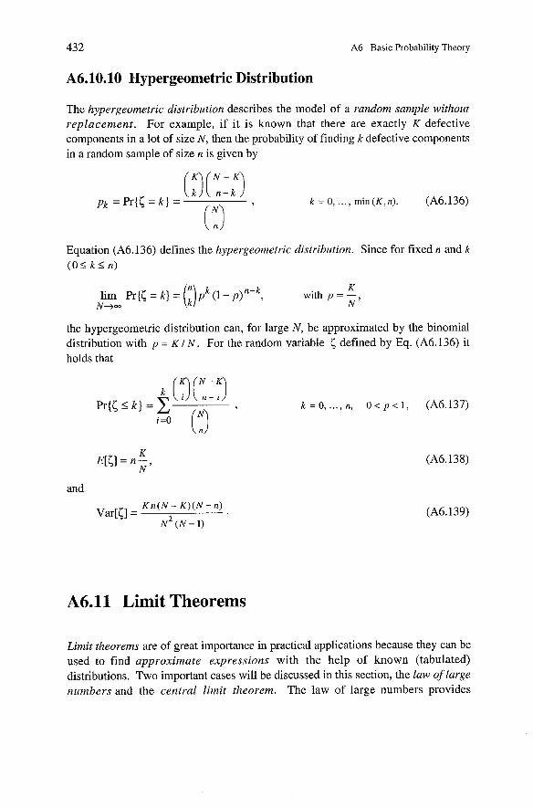
432 A6 Basic Probability Theory
A6.10.10 Hypergeometric Distribution
The hypergeometric distribution describes the model of a random sample without replacement. For example, if it is known that there are exactly K defective components in a lot of size N , then the probability of finding k defective components in a random sarnple of size n is given by
pk =Pr{[= k } = (3 (1 kK) 9
k = 0, . . . , min ( K , n). (A6.136)
Equation (A6.136) defines the hypergeometric distribution. Since for fixed n and k ( 0 5 k l n )
lim Pr{[ = k } = ( i ) p k ( l - p ) n - k , K
with p = -, N+m N
the hypergeometric distribution can, for large N, be approximated by the binomial distribution with p = K I N . For the random variable 5 defined by Eq. (A6.136) it holds that
and
A6.11 Limit Theorems
Limit theorems are of great importance in practical applications because they can be used to find approximate expressions with the help of known (tabulated) distributions. Two important cases will be discussed in this section, the law of Zarge numbers and the central limit theorem. The law of large numbers provides
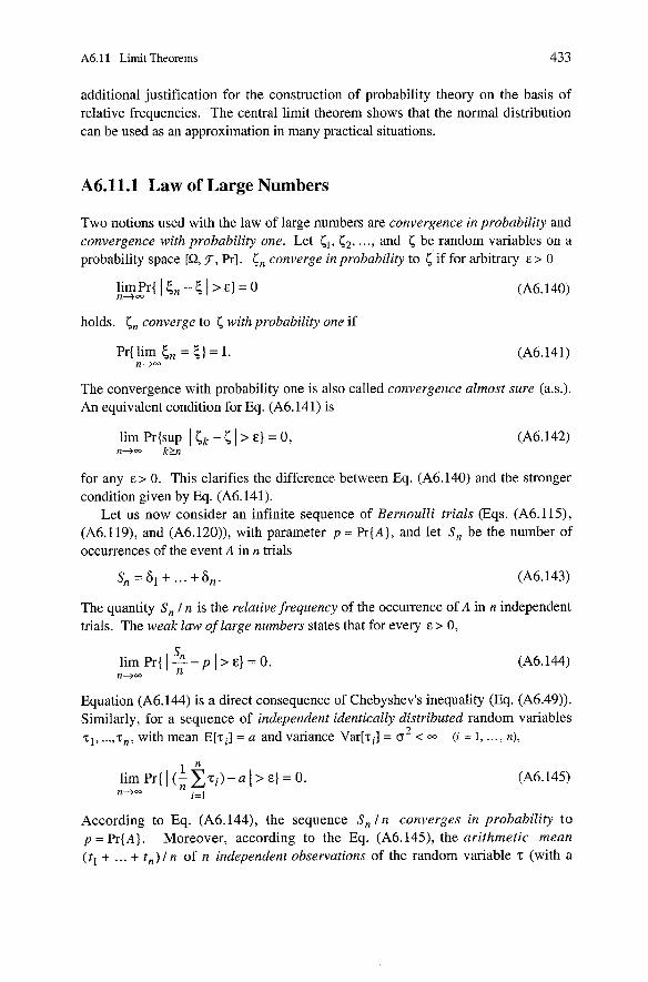
A6.11 Limit Theorems 433
additional justification for the construction of probability theory on the basis of relative frequencies. The central limit theorem shows that the normal distribution can be used as an approximation in many practical situations.
A6.11.1 Law of Large Nurnbers
Two notions used with the law of large numbers are convergence in probability and convergence with probability one. Let Cl, c2, . . ., and 5 be random variables on a probability space [Q, F, Pr]. 5, converge in probability to 5 if for arbitrary E > 0
holds. 5, converge to 5 with probability one if
The convergence with probability one is also called convergence almost sure (a.s.). An equivalent condition for Eq. (A6.141) is
lim Pr{sup -< I>& } = 0, n k>n
for any E > 0. This clarifies the difference between Eq. (A6.140) and the stronger condition given by Eq. (A6.141).
Let us now consider an infinite sequence of Bernoulli trials (Eqs. (A6.115), (A6.119), and (A6.120)), with Parameter p = P r { A ) , and let S n be the number of occurrences of the event A in n trials
The quantiiy S n I n is the relative frequency of the occurrence of A in n independent trials. The weak law of large numbers states that for every E > 0,
Equation (A6.144) is a direct consequence of Chebyshev's inequality (Eq. (A6.49)). Similarly, for a sequence of independent identically distributed random variables
2 z l , ..., T „ with mean E [ z i ] = a and variance Var[ z i ] = o < m (i = 1, ... , n),
According to Eq. (A6.144), the sequence S n l n converges in probability to p = Pr{A]. Moreover, according to the Eq. (A6.145), the arithmetic mean ( t l + ... + t n ) l n of n independent obsewations of the random variable T (with a
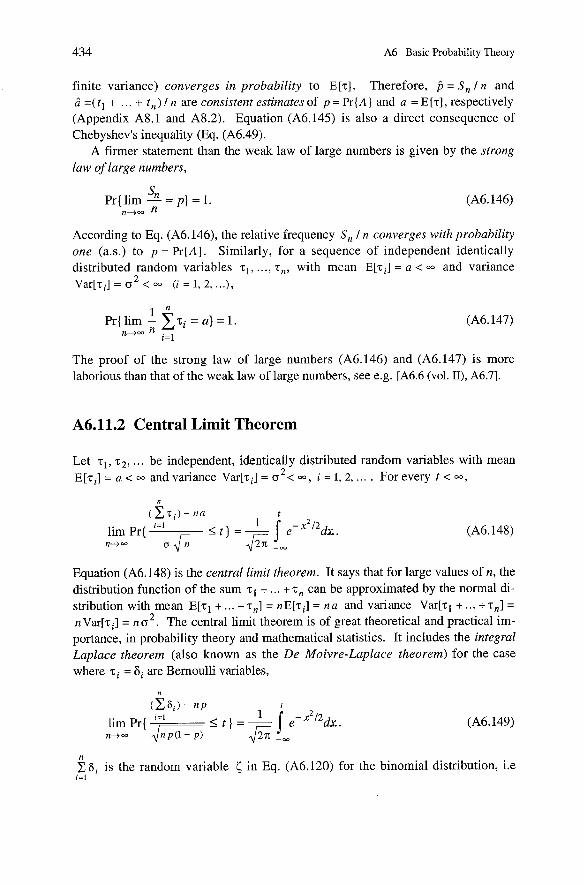
434 A6 Basic Probability Theory
finite variance) converges in probability to E [ z ] . Therefore, 6 = Sn 1 n and 6 =(tl + ... + t,)l n are consistent estimatesof p = Pr{A) and a = E [ z ] , respectively (Appendix A8.1 and A8.2). Equation (A6.145) is also a direct consequence of Chebyshev's inequality (Eq. (A6.49).
A firmer statement than the weak law of large numbers is given by the strong law of large numbers,
According to Eq. (A6.146), the relative frequency S n I n converges with probability one (a.s.) to p = Pr{A} . Similarly, for a sequence of independent identically distributed random variables z l , . . ., T „ with mean E[z i ] = a < and variance
2 V a r [ z i ] = o < W ( i=1 ,2 , ...),
The proof of the strong law of large numbers (A6.146) and (A6.147) is more laborious than that of the weak law of large numbers, see e.g. [A6.6 (vol. 11), A6.71.
A6.11.2 Central Limit Theorem
Let T I , T Z , ... be independent, identically distributed random variables with mean 2 E [ z i ] = a < W andvariance V a r [ ~ ~ ] = o < W , i = 1,2 , ... . For every t C W ,
( C ~ ~ ) - n a t i=l 1
lim Pr{ ,- x2/zdX
n+ -= 4 Equation (A6.148) is the central limit theorem. It says that for large values of n, the distribution function of the sum z l + ... + T , can be approximated by the normal di- stribution with mean E[z l + ... + z n ] = n E [ z i ] = n a and variance Var[zl + ... +T,] =
nVar[z i] = n o 2 . The central limit theorem is of great theoretical and practical im- portance, in probability theory and mathematical statistics. It includes the integral Laplace theorem (also known as the De Moivre-Laplace theorem) for the case where z i = Zii are Bernoulli variables,
n C 6 , is the random variable 5 in Eq. (A6.120) for the binomial distribution, i.e i = l
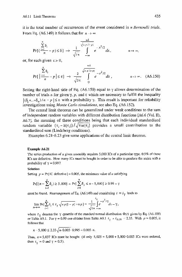
A6.11 Limit Theorems 435
it is the total number of occurrences of the event considered in n Bernoulli trials.
From Eq. (A6.149) it follows that for n + n F z si 1 ,lzG - x2/2
81 -+ - I e d'. n+ W,
2j211 -m
or, for each given E > 0, II E
X 8, 2
G= -x2,2
P - I } -+ - J e h, n- t W . (A6.150) li.. ,
Setting the right-hand side of Eq. (A6.150) equal to y allows determination of the number of trials n for given y, p, and E which are necessary to fulfill the inequality 1(4 +...+ 8,) l n - p I I E with a probability y. This result is important for reliability investigations using Monte Carlo simulations, see also Eq. (A6.152).
The central limit theorem can be generalized under weak conditions to the sum of independent random variables with different distribution functions [A6.6 (Vol. 11), A6.71, the meaning of these conditions being that each individual standardized random variable ( z i - E [ z i ] ) /,,/M provides a small contribution to the standardized sum (Lindeberg conditions).
Examples 6.21-6.23 give some applications of the central limit theorem.
Example A6.21
The senes production of a given assembly requires 5,000 ICs of a particular type. 0.5% of these ICs are defective. How many ICs must be bought in order to be able to produce the series with a probability of y = 0.99?
Solution Setting p = Pr{IC defective} = 0.005, the minimum value of n satisfying
i=l i=l
must be found. Rearrangement of Eq. (A6.149) and considering t = t y leads to
where t y denotes the y quantile of the standard normal distribution @(t) given by Eq. (A6.109) or Table A9.1. For y = 0.99 one obtains from Table A9.1 t,, = to,99 = 2.33. With p = 0.005, it follows that
Thus, n = 5,037 ICs must be bought (if only 5,025 = 5,000 + 5,000.0.005 ICs were ordered, then t y = 0 and y = 0.5).
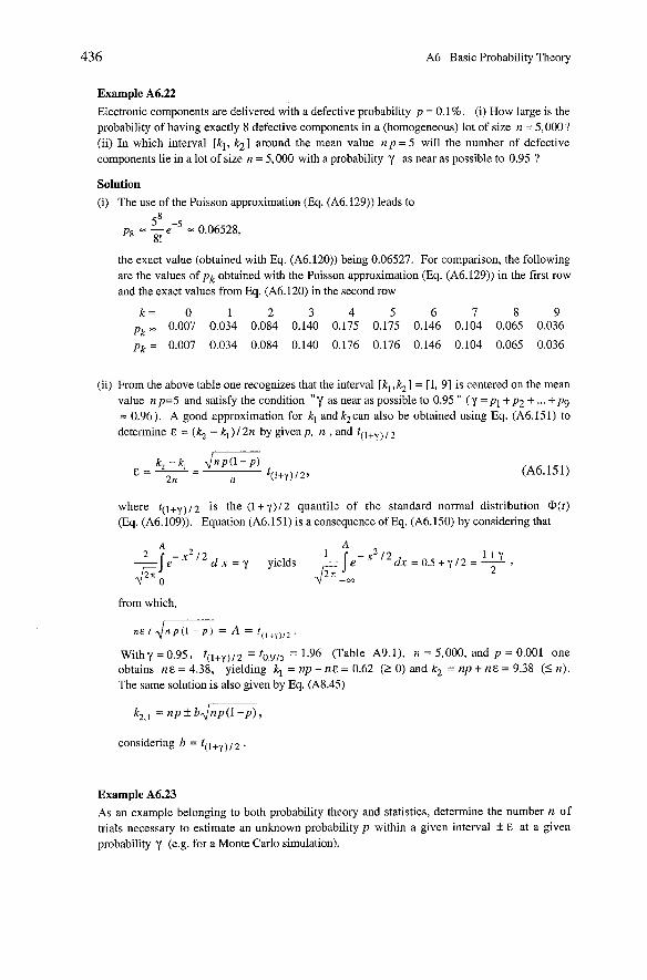
A6 Basic Probability Theory
Example A6.22 Electronic components are delivered with a defective probability p = 0.1%. (i) How large is the probability of having exactly 8 defective components in a (homogeneous) lot of size n = 5,000? (ii) In which interval [kl, k2] around the mean value n p = 5 will the number of defective components lie in a lot of size n = 5,000 with a probability Y as near as possible to 0.95 ?
Solution
(i) The use of the Poisson approximation (Eq. (A6.129)) leads to
the exact value (obtained with Eq. (A6.120)) being 0.06527. For comparison, the following are the values of pk obtained with the Poisson approximation (Eq. (A6.129)) in the first row and the exact values from Eq. (A6.120) in the second row
(ii) From the above table one recognizes that the interval [kl, k2] = [I, 91 is centered on the mean value n p=5 and satisfy the condition ''Y as near as possible to 0.95 " ( y = pl + p2 + ... + pg - 0.96). A good approximation for kl and k2can also be obtained using Eq. (A6.151) to determine E = (k2 - k,)l2n by given p, n , and t(l+y)
where t ( l + y ) / 2 is the (1 + y ) / 2 quantile of the standard normal distribution @(t) (Eq. (A6.109)). Equation (A6.151) is a consequence of Eq. (A6.150) by considering that
from which,
n E I - , /np( l - P ) = A = t(,+y),2.
Withy = 0.95, t(l+y)12 = tO,„, = 1.96 (Table A9.1), n = 5,000, and p = 0.001 one obtains n& = 4.38, yielding kl = np - nE = 0.62 (2 0) and kz = np + n & = 9.38 (5 n). The same solution is also given by Eq. (A8.45)
considering b = t(l+y) .
Example A6.23 As an example belonging to both probability theory and statistics, determine the number n of hials necessary to estimate an unknown probability p within a given interval f E at a given probability Y (e.g. for a Monte Carlo simulation).
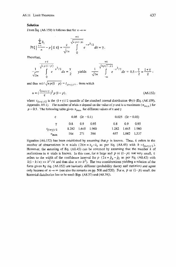
A6.11 Limit Theorems
Solution From Eq. (A6.150) it follows that for n -t
Therefore, n E nE
1 - Y 1 I e dx = - yields - Y l + y
2 6 e dx=O.5+-=- , 2 2
-m
and thus n e l Jnp(l-p) = t ( „y)12 , from which
where t(l+y)12 is the (1 + y ) l 2 quantile of the Standard normal distribution @(t ) (Eq. (A6.109), Appendix A9.1). The number of trials n depend on the value of p and is a maximum ( nmX ) for p = 0.5. The following table gives n„, for different values of E and y
Equation (A6.152) has been established by assuming that p is known. Thus, E refers to the number of observations in n trials (2En = k2-k, as per Eq. (A8.45) with b = t(l+y)12). However, the meauing of Eq. (A8.45) can be reversed by assuming that the number k of realizations in n trials is known. In this case, for n large and p or (1 - p ) not very small, E
refers to the width of the confidence interval for p (28 = 6, - P l as per Eq. (A8.43) with k(1- k l n) >> b2 I 4 and thus also n >> b2). The two considerations yielding a relation of the form given by Eq. (A6.152) are basically different (probability theory and statistics) and agree only because of n -t W (see also the remarks on pp. 508 and 520). For n, p or (1 - p ) small, the binomial distribution has to be used (Eqs. (A8.37) and (A8.38)).
A7 Basic Stochastic-Processes Theory
Stochastic processes are a powerful tool for investigating reliability and availability of repairable equipment and Systems. A stochastic process can be considered as a family of time-dependent random variables or as a random function in time, and thus has a theoretical foundation based on probability theory (Appendix A6). The use of stochastic processes allows analysis of the influence of the failure-free and repair time distributions of elements, as well as of the system's structure, repair strategy, and logistic support, on the reliability and availability of a given system. Considering applications given in Chapter 6, this appendix mainly deals with regenerative stochastic processes with a finite state space, to which belong renewal processes, Markov processes, semi-Markov processes, and semi-regenerative proc- esses, including reward and frequencylduration aspects. However, because of their importance, some nonregenerative processes (in particular the nonhomogeneous Poisson process) are introduced in Appendix A7.8. This appendix is a compendium of the theory of stochastic processes, consistent from a mathematical point of view but still with reliability engineering applications in mind. Selected examples illustrate the practical aspects.
A7.1 Introduction
Stochastic processes are mathematical models for random phenomena evolving over time, such as the time behavior of a repairable system or the noise voltage of a diode. They are designated hereafter by Greek letters g(t) , C( t ) , q ( t ) , ~ ( t ) etc.
To introduce the concept of stochastic process, consider the time behavior of a system subject to random influences and let T be the time interval of interest, e.g. T = [O, m). The Set of possible states of the system, i.e. the state space, is assumed to be a subset of the set of real numbers. The state of the system at a given time to is thus a random variable & t o ) The random variables Q t ) , t E T , may be arbitrarily coupled together. However, for any n = 1,2, ..., and arbitrary values t l , ..., t , E T , the existence of the n-dimensional distributionfunction (Eq. (A6.51))
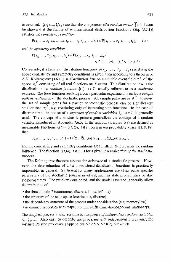
A7.1 Introduction 439
is assumed. {(tl), ..., <(tn) are thus the components of a random vector l ( t ) . It can be shown that the family of n-dimensional distribution functions (Eq. (A7.1)) satisfies the consistency condition
F(xl, . . ., xk,m, . . ., W, tl, . . . , tk,tk+l, . . ., t,) = F(xl, . . ., xk, tl, . . ., tk), k < n
Conversely, if a family of distribution functions F ( x l , ..., X„ t l , ..., t, ) satisfying the above consistency and symmetry conditions is given, then according to a theorem of A.N. Kolmogorov [A6.10], a distribution law on a suitable event field of the space $T consisting of all real functions on T exists. This distribution law is the distribution of a random function {(t), t E T, usually referred to as a stochastic process. The time function resulting from a particular experiment is called a sample path or realization of the stochastic process. All sample paths are in $ T , however the set of sample paths for a particular stochastic process can be significantly smaller than $ T , e.g. consisting only of increasing step functions. In the case of discrete time, the notion of a sequence of random variables C„ n G T is generally used. The concept of a stochastic process generalizes the concept of a random variable introduced in Appendix A6.5. If the random variables {(t) are defined as measurable functions <(t) = <(t, W), t E T, on a given probability space [G, F, Pr] then
F(xl, . . ., X„ tl, . .., tn) = Pr{o : E,(tl,o) 5 xl, . . ., 5(t„w) I X,},
and the consistency and symmetry conditions are fulfilled. o represents the random influence. The function { ( t , ~ ) , t E T, is for a given W a realization of the stochastic process.
The Kolmogorov theorem assures the existence of a stochastic process. How- ever, the determination of all n-dimensional distribution functions is practically impossible, in general. Sufficient for many applications are often some specific Parameters of the stochastic process involved, such as state probabilities or stay (sojourn) times. The problem considered, and the model assumed, generally allow deterrnination of
the time domain T (continuous, discrete, finite, infinite) the structure of the state space (continuous, discrete) the dependency structure of the process under consideration (e.g. memoryless) invariance properties with respect to time shifts (time-homogeneous, stationary).
The simplest process in discrete time is a sequence of independent random variables Ci, t2, . . . . Also easy to describe are processes with independent increments, for instance Poisson processes (Appendices A7.2.5 & A7.8.2), for which
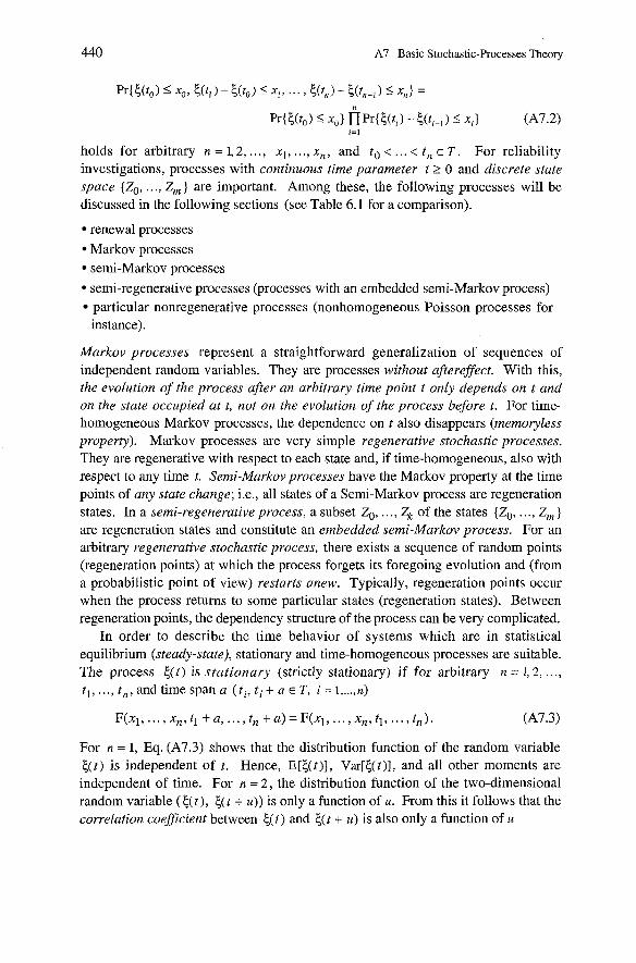
440 A7 Basic Stochastic-Processes Theory
II
pr{t(to) 5 X,} n p r { t ( t i ) - t(ti-~) 5 (A7.2) i = l
holds for arbitrary n = 1,2, ..., XI, ..., X , , and to < ... < t , E T . For reliability investigations, processes with continuous time Parameter t 2 0 and discrete state space {Zo, ..., Ztn) are important. Among these, the following processes will be discussed in the following sections (see Table 6.1 for a comparison).
renewal processes
Markov processes semi-Markov processes
semi-regenerative processes (processes with an embedded semi-Markov process) particular nonregenerative processes (nonhomogeneous Poisson processes for instance).
Markov processes represent a straightforward generalization of sequences of independent random variables. They are processes without aftereffect. With this, the evolution of the process after an arbitrary time point t only depends on t und on the state occupied at t, not on the evolution of the process before t. For time- homogeneous Markov processes, the dependence on t also disappears (memoryless propers). Markov processes are very simple regenerative stochastic processes. They are regenerative with respect to each state and, if time-homogeneous, also with respect to any time I. Semi-Markov processes have the Markov property at the time points of any state change; i.e., all states of a Semi-Markov process are regeneration states. In a semi-regenerative process, a subset Zo, . . ., Zk of the states {Zo, . . ., Z, )
are regeneration states and constitute an embedded semi-Markov process. For an arbitrary regenerative stochastic process, there exists a sequence of random points (regeneration points) at which the process forgets its foregoing evolution and (from a probabilistic point of view) restarts anew. Typically, regeneration points occur when the process returns to some particular states (regeneration states). Between regeneration points, the dependency stmcture of the process can be very complicated.
In order to describe the time behavior of Systems which are in statistical equilibrium (steady-state), stationary and time-homogeneous processes are suitable. The process { ( t ) is stationary (strictly stationary) if for arbitrary n = 1,2, ..., t l , ..., t„ and time span a ( t i , ti + a E T , i = i ,..., n)
F(xl, . . . , X,, tl + U, . . . , t, + U ) = F(xl, . . . , X„ tl, . . . , t , ) . (A7.3)
For n = 1, Eq. (A7.3) shows that the distribution function of the random variable c ( t ) is independent of t . Hence, E[ t ( t ) ] , Var[C(t)], and all other moments are independent of time. For n = 2, the distribution function of the two-dimensional random variable ( & t ) , { ( t + U)) is only a function of U. From this it follows that the correlation coeflcient between { ( t ) and t ( t + U) is also only a function of u
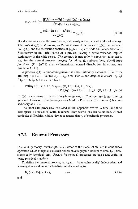
A7.1 Introduction
Besides stationarity in the strict sense, stationarity is also defined in the wide sense. The process & t ) is stationary in the wide sense if the mean E[t(t)] the variance Var[<(t)], and the correlation coefficient ptS(t,t + U) are finite and independent oft. Stationarity in the strict sense of a process having a finite variance implies stationarity in the wide sense. The contrary is true only in some particular cases, e.g. for the normal process (process for which all n-dimensional distribution finctions (Eq. (A7.1) are n-dimensional normal distribution functions, See Example A6.16).
A process c(t) is time-homogeneous if it has stationary increments, i.e. if for arbitrary n = L2, ..., values X,, ..., X„ time Span a, and disjoint intervals ( ti, bi) ((ti, ti + a, bi, bi + a E T, i = 1 ,..., n )
If c(t) is stationary, it is also time-homogeneous. The contrary is not true, in general. However, time-homogeneous Markov Processes (for instance) become stationary as t -1 W .
The stochastic processes discussed in this appendix evolve in time, and their state space is a subset ofnatural numbers. Both restrictions can be omitted, without particular difficulties, with a view to a general theory of stochastic processes.
A7.2 Renewal Processes
In reliability theory, renewal processes describe the model of an item in continuous operation which is replaced at each failure, in a negligible amount of time, by a new, statistically identical item. Results for renewal processes are basic and useful in many practical situations.
To define the renewal process, let T ~ , T ~ , ... be (stochastically) independent and non-negative random variables distributed according to
FA(x) = Pr{zO 5 X}, x2.0,
and
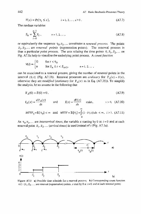
A7 Basic Stochastic-Processes Theory
i = I , 2, ..., x > O . (A7.7)
The random variables
or equivalently the sequence q , , ~ l , ... constitutes a renewal process. The points S I , S 2 , ... are renewal points (regeneration points). The renewal process is thus a particular point process. The arcs relating the time points 0, SI, S2, . . . on Fig. A7.la help to visualize the underlying point process. A count function
can be associated to a renewal process, giving the number of renewal points in the interval ( 0 , t] (Fig. A7.lb). Renewal processes are ordinary for F A ( 2 ) = F ( x ) , otherwise they are modified (stationary for F A ( x ) as in Eq. (A7.35)). To simplify the analysis, let us assume in the following that
m
M7TFo=E[r,] < W and M n F = E [ r J = / ( I - F ( x ) ) & < -, i n 1. (A7.11) 0
As zo , z l , . .. are interarrival times, the variable x starting by 0 at t = 0 and at each renewal point S I , S2, . .. (arrival times) is used instead o f t (Fig. A7.la).
Figure A7.1 a) Possible time schedule for a renewal process; b) Corresponding count function v(t) (Si, SZ, . . . are renewal (regeneration) points, X start by 0 at t = 0 and at each renewal point)
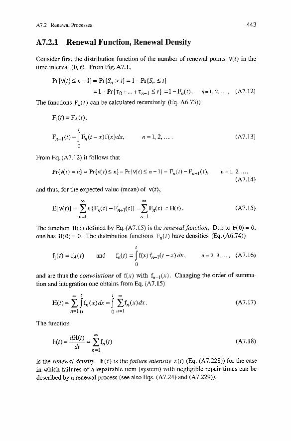
A7.2 Renewal Processes 443
A7.2.1 RenewaI Function, Renewal Density
Consider first the distribution function of the number of renewal points v(t) in the time interval (0, t] . From Fig. A7.1,
Pr{v(t) I n-1}= Pr{& > t} = 1-Pr(& I t}
= l - P r { ~ ~ + ...+ ~ ~ - ~ S t ] = 1 - F , ( t ) , n = 1 , 2 ,.... (A7.12)
The functions FJt) can be calculated recursively (Eq. A6.73))
From Eq. (A7.12) it follows that
and thus, for the expected value (mean) of ~ ( t ) ,
The function H(t) defined by Eq. (A7.15) is the renewal function. Due to F(0) = 0, one has H(0) = 0. The distribution functions FJt) have densities (Eq. (A6.74))
t
fl(t) = fA(t) and f,(t) = 1 f(r) fn-l(t -X) dr , n = 2, 3, . . . , (A7.16) 0
and are thus the convolutions of f(x) with fn-l(x). Changing the order of summa- tion and integration one obtains from Eq. (A7.15)
The function
&(t> - M
h(t) = - - C fn (t) dt n=l
is the renewal density. h( t ) is the failure intensity z (t) (Eq. (A7.228)) for the case in which failures of a repairable item (system) with negligible repair times can be described by a renewal process (see also Eqs. (A7.24) and (A7.229)).
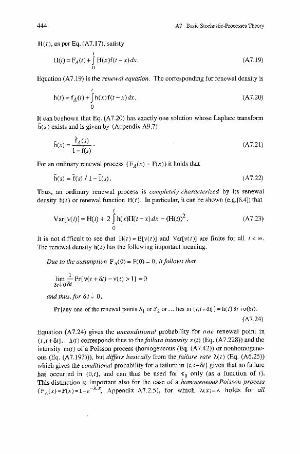
444 A7 Basic Stochastic-Processes Theory
H(t), as per Eq. (A7.17), satisfy
Equation (A7.19) is the renewal equation. The corresponding for renewal density is
It can be shown that Eq. (A7.20) has exactly one solution whose Laplace transform i(s) exists and is given by (Appendix A9.7)
For an ordinary renewal process (FA(x) = F(x)) it holds that
Thus, an ordinary renewal process is completely characterized by its renewal density h(t) or renewal function H(t). In particular, it can be shown (e.g.[6.4]) that
t
~ a r [ v ( t ) ] = ~ ( t ) + 2 j h ( x ) ~ ( t - X) dx - ( ~ ( t ) ) ~ . (A7.23) 0
It is not difficult to see that H(t) = E[v(t)] and Var[v(t)] ase finite for all t < W .
The renewal density h(t) has the following important meaning:
Due to the assumption FA(0) = F(0) = 0, it follows that
1 lim - Pr{v(t + 8t) - v(t) > 1) = 0 stLo6t
und thus, for 8 t -1 0,
Pr {any one of the renewal points SI or S2 or . . . lies in ( t , t + Ft] } = h(t) F t +o(Ft) . (A7.24)
Equation (A7.24) gives the unconditional probability for one renewal point in ( t , t +&I. h(t) corresponds thus to the failure intensity z (t) (Eq. (A7.228)) and the intensity m(t) of a Poisson process (homogeneous (Eq. (A7.42)) or nonhomogene- ous (Eq. (A7.193))), but differs basically from the failure rate h(t) (Eq. (A6.25)) which gives the conditional probability for a failure in (t,t +8t] given that no failure has occurred in (O,t], and can thus be used for only (as a function of t). This distinction is important also for the case of a homogeneous Poisson process (F*(x) = ~ ( x ) = 1 -e-hX, Appendix A7.2.5), for which h(x)=h holds for all
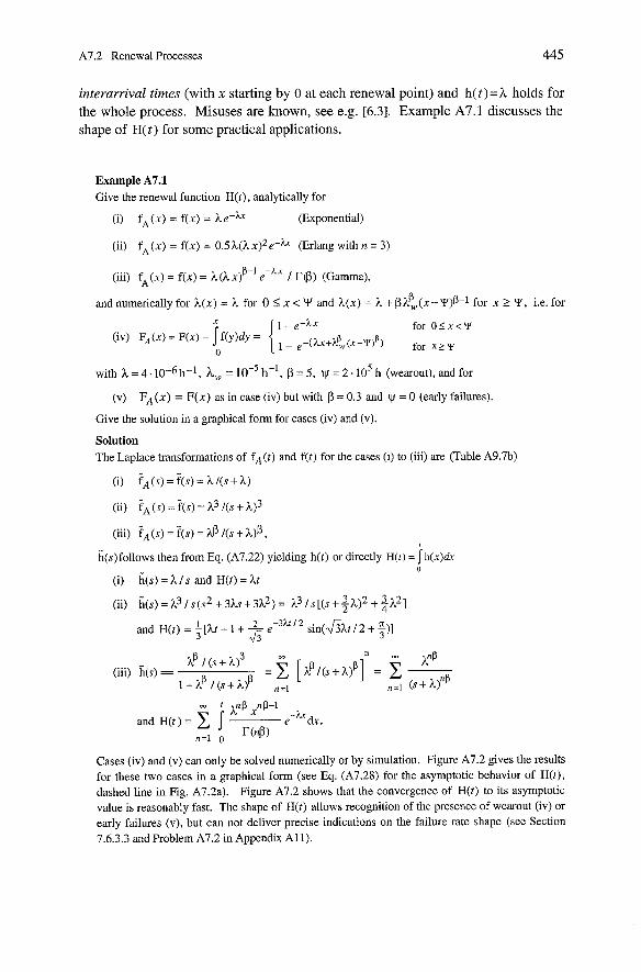
A7.2 Renewal Processes 445
interarrival times (with X starting by 0 at each renewal point) and h ( t ) = h holds for the whole process. Misuses are known, See e.g. [6.3]. Example A7.1 discusses the shape of H(t) for some practical applications.
Example A7.1 Give the renewal function H(t), analytically for
(i) f, (X) = f(x) = h echx (Exponential)
(ii) fA(x) = f(x) = 0.5 h(h x)2e-hx (Erlang with n = 3)
(iii) fA (X) = f(x) = h (h xf l e-hx / r@) (Gamma),
and numerically for h(x) = h for 0 5 X < Y and h(x) = h + ßhß , (x -~ )ß - l for x 2 Y, i.e. for
with h = 4.10-~ h-l, h w = 10-~ h-', ß = 5, W = 2.10' h (wearout), and for
(V) FA ( X ) = F(x) as in case (iv) but with ß = 0.3 and = 0 (early failures).
Give the solution in a graphical form for cases (iv) and (V).
Solution The Laplace transformations of fA (t) and f(t) for the cases (i) to (iii) are (Table A9.7b)
(ii) TA (s) = F(s) = h3 /(S + h13
(iii) FA (s) = f(s) = Aß I(s + h)ß , I
i(s)follows then from Eq. (A7.22) yielding h(t) or directly H(t) = h(x)dx 0
(i) i(s) = h 1 s and H(t) = ht
(ii) h ( s ) = h 3 / ~ ( ~ 2 + 3 h s + 3 h 2 ) = h 3 1 s [ ( s + ~ h ) ~ + $ h ~ ]
and H(t) = :[ht - 1 + 2- e-3)3'2 sin(yl3htt 2 + :)I 113 hß 1 (S + h)'
n m
(iii) h(s) == hnß = E [ h ~ l ( s + h ) ß ] = C --
i - h ß / ( s + h ) ß .=I ,,=I (S + hY"'
t n ß nß-1 h X -h
and H(t )= --- e dx. ,, '("B)
Cases (iv) and (V) can only be solved numerically or by simulation. Figure A7.2 gives the results for these two cases in a graphical form (see Eq. (A7.28) for the asymptotic behavior of H(t), dashed line in Fig. A7.2a). Figure A7.2 shows that the convergence of H(t) to its asymptotic value is reasonably fast. The shape of H(t) allows recognition of the presence of wearout (iv) or early failures (V), but can not deliver precise indications on the failure rate shape (see Section 7.6.3.3 and Problem A7.2 in Appendix Al l ) .
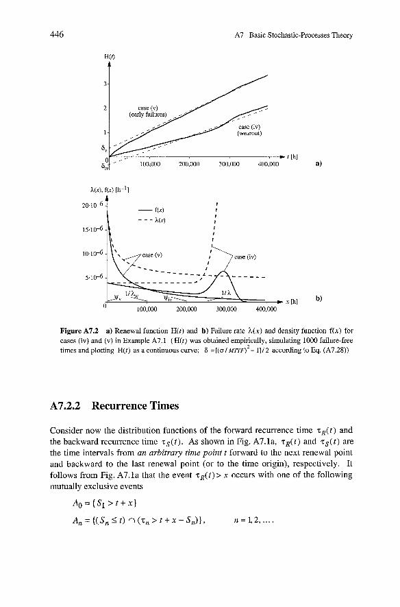
446 A7 Basic Stochastic-Processes Theory
Figure A7.2 a) Renewal function H(t) and b) Failure rate h(x) and density function f(x) for cases (iv) and (V) in Example A7.1 (H(t) was obtained empirically, simulating 1000 failure-free times and plotting H(t) as a continuous curve; 6 =[(a / MZTF)' - I]/ 2 according to Eq. (A7.28))
A7.2.2 Recurrence Times
Consider now the distribution functions of the fonvard recurrence time ~ ~ ( t ) and the backward recurrence time z s ( t ) . As shown in Fig. A7. la, T,( t ) and ~ , ( t ) are the time intervals from an arbitrary time point t forward to the next renewal point and backward to the last renewal point (or to the time origin), respectively. It follows from Fig. A7.la that the event ~ ~ ( t ) > X occurs with one of the following mutually exclusive events
A o = { S 1 > t + x }
An = {(Sn I t ) n (7, > t + X - Sn)} , n = l,2, ... .
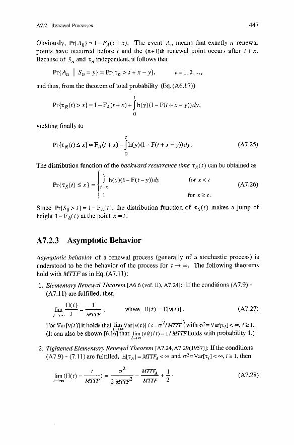
A7.2 Renewal Processes 447
Obviously, Pr{Ao} = 1 - FA(t + X). The event An means that exactly n renewal points have occurred before t and the (n+l)th renewal point occurs after t + x. Because of Sn and T, independent, it follows that
Pr{& I Sn = y} = Pr{z, > t + x - y}, n = 1, 2, ...,
and thus, from the theorem of total probability (Eq. (A6.17))
yielding finally to
t
Pr{~,( t )Sx]=F~(t+x)-Jh(y)( l-F(t+x-y))dy. (A7.25) 0
The distribution function of the backward recurrence time zS(t) can be obtained as
Since Pr{SO > t} = 1 - FA(t), the distribution function of zs(t) makes a jump of height 1 - FA(t) at the point x = t .
A7.2.3 Asymptotic Behavior
Asymptotic behavior of a renewal process (generally of a stochastic process) is understood to be the behavior of the process for t + W . The following theorems hold with MTTF as in Eq. (A7.11):
1. Elementary Renewal Theorem [A6.6 (vol. 11), A7.241: If the conditions (A7.9) - (A7.11) are fulfilled, then
H(t) - 2 lim - - where H(t) = E[v(t)] . t+- t MTTF'
3 For Var[v(t)] it holds that /ltVar[v(t)] / t = 02/ MVF , with 02=Var[ri] < W, i 2 1.
(It can also be shown [6.16] that lim (V@)/ t ) = 1 / MTTFholds with probability 1.) t+-
2. Tightened Elementary Renewal Theorem [A7.24, A7.29(1957)]: If the conditions (A7.9) - (7.1 1) are fulfilled, E[z,] = M- < and 0 2 = Var[.ci] < W, i 2 I, then
t Ci M T 1 lim (H(t) - -) = - - - + - . (A7.28) t+- MTTF 2~7777' M?TF 2
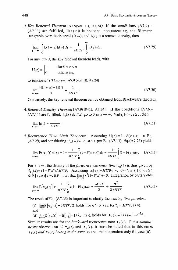
448 A7 Basic Stochastic-Processes Theory
3.Key Renewal Theorem [A7.9(vol. 11), A7.241: If the conditions (A7.9) - (A7.11) are fulfilled, U ( z ) 2 0 is bounded, nonincreasing, and Riemann integrable over the interval (0, W), and h ( t ) is a renewal density, then
lim t+=
For any a > 0, the key renewal theorem leads, with
(1 f o r O < z < a = 10 oiherwise,
to Blackwell's Theorem rA7.9 (vol. 11), A7.241
H ( t + a ) - H ( t ) 1 lim -- -
t+- a M n F
Conversely, the key renewal theorem can be obtained from Blackwell's theorem.
4.Renewal Density Theorem [A7.9(1941), A7.241: If the conditions (A7.9)- (A7.11) are fulfilled, f A ( x ) & f ( x ) go to 0 as X -+ Var[.ti] < W, i 2 1, then
1 lim h(t) = -.
M7TF (A7.31)
t+-
5. Recurrence Time Limit Theorems: Assuming U ( z ) = 1 - F(x + z ) in Eq. (A7.29) and considering F A ( - ) = 1 & MTTF per Eq. (A7.1 I), Eq. (A7.25) yields
rn 1 1 X
iimPr{.tR(r)<x)=l--J(1-F(x+z))dz=-/(I-F(y))dyi (A7.32) t+- MTTF MTTF
For t -+ -, the density of the fonvard recurrence time z R ( t ) is thus given by fTR(x)= ( 1 - F(x)) I MiTF. Assuming E [ T ~ ] = M ~ F < W , 02=Var[.ti]< W, i t 1
& E [ T , (t )]< -, it follows that lim (x2(1-F(x)))= 0 . Integration by parts yields X-f -
CG
1 MTTF 0 2
iim E[.tR(t)] = -J ~ ( 1 - F ( x ) ) & = - + - . t+- MTTF 2 2 MTTF
The result of Eq. (A7.33) is important to clarify the waiting time paradox :
(i) ?L%E [.tR(t)] = MTTF 12 holds for oZ=O (is. for 'Ti = MTTF, i tO) , and
-hx (ii) &E [.tR(t)] = E [ z i ] = 1 I h, i 2 0, holds for F,(x) = F(x) = 1 - e . Similar results are for the backward recurrence time z S ( t ) . For a simulta- neous observation of z R ( t ) and z s ( t ) , it must be noted that in this cases z R ( t ) und . tS ( t ) belong to the same zi and are independent only for case (ii).
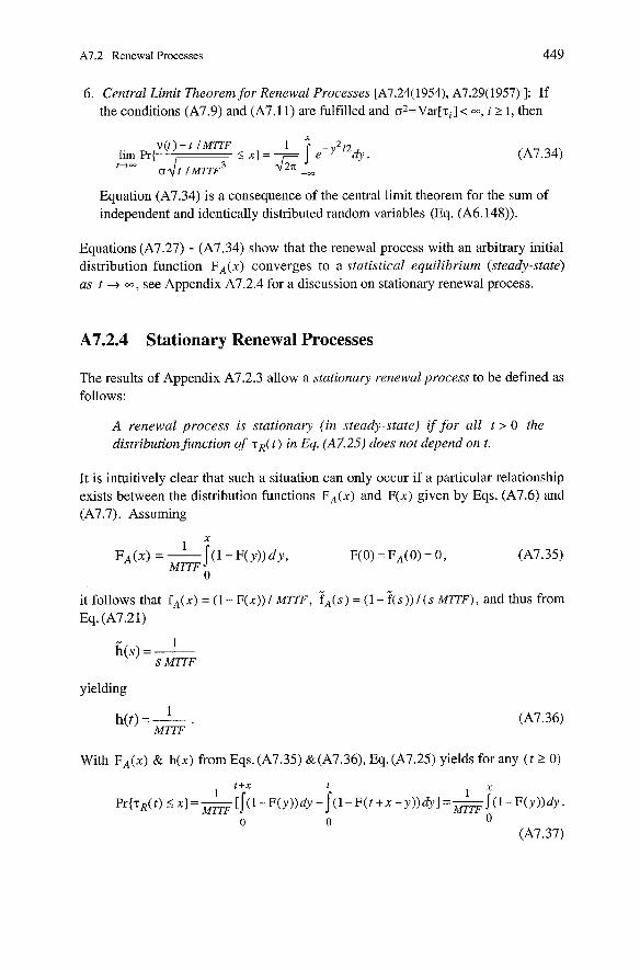
A7.2 Renewal Processes 449
6. Central Limit Theorem for Renewal Processes [A7.24(1954), A7.29(1957) 1: If the conditions (A7.9) and (A7.11) are fulfilled and 02=Var[xi] < -J, i 2 1, then
Equation (A7.34) is a consequence of the central limit theorem for the sum of independent and identically distributed random variables (Eq. (A6.148)).
Equations (A7.27) - (A7.34) show that the renewal process with an arbitrary initial distribution function FA(x) converges to a statistical equilibrium (steady-state) as t -+ W , see Appendix A7.2.4 for a discussion on stationary renewal process.
A7.2.4 Stationary Renewal Processes
The results of Appendix A7.2.3 allow a stationary renewal process to be defined as follows:
A renewal process is stationary (in steady-state) if for all t 0 the distributionfunction of ~ ~ ( t ) in Eq. (A7.25) does not depend on t.
It is intuitively clear that such a situation can only occur if a particular relationship exists between the distribution functions FA(x) and F(x) given by Eqs. (A7.6) and (A7.7). Assuming
it follows that fA(x ) = (1 - F(x)) l m F , i A ( s ) = ( 1 - f ( s ) ) / ( s MTTF) , and thus from Eq. (A7.21)
- 1 h(s) = -
S MTTF
yielding
1 h(t) = - .
MTTF
With FA(") & h(x) from Eqs. (A7.35) &(A7.36), Eq. (A7.25) yields for any ( t 2 0 )
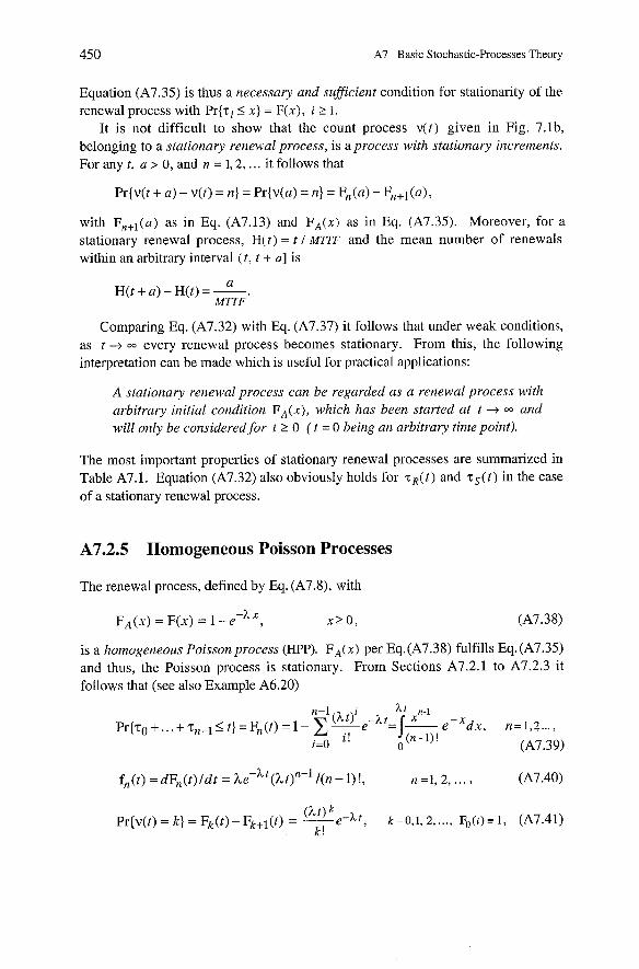
450 A7 Basic Stochastic-Processes Theory
Equation (A7.35) is thus a necessary und sufficient condition for stationarity of the renewal process with Pr{zi 5 X ) = F(x), i 2 1.
It is not difficult to show that the Count process v ( t ) given in Fig. 7.lb, belonging to a stationary renewal process, is a process with stationary increments. For any t, a > 0, and n = 1,2, ... it follows that
with F„l(a) as in Eq. (A7.13) and FA(x) as in Eq. (A7.35). Moreover, for a stationary renewal process, H(t ) = t l MTTF and the mean number of renewals within an arbitrary interval ( t , t + U ] is
Comparing Eq. (A7.32) with Eq. (A7.37) it follows that under weak conditions, as t -+ every renewal process becomes stationary. From this, the following interpretation can be made which is useful for practical applications:
A stationary renewal process can be regarded as a renewal process with arbitrary initial condition FA(x), which has been started at t 4 und will only be considered for t > 0 ( t = 0 being an arbitrary time point).
The most important properties of stationary renewal processes are summarized in Table A7.1. Equation (A7.32) also obviously holds for z R ( t ) and z s ( t ) in the case of a stationary renewal process.
A7.2.5 Homogeneous Poisson Processes
The renewal process, defined by Eq. (A7.8), with
is a homogeneous Poisson process (HPP). FA(x) per Eq.(A7.38) fulfills Eq. (A7.35) and thus, the Poisson process is stationary. From Sections A7.2.1 to A7.2.3 it follows that (see also Example A6.20)
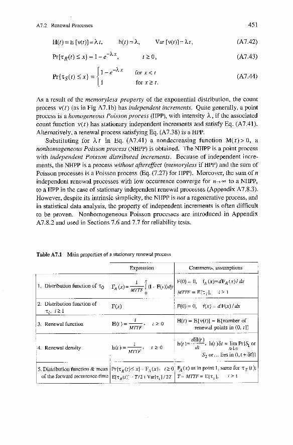
A7.2 Renewal Processes 45 1
As a result of the merno~less property of the exponential distribution, the count process v(t) (as in Fig A7.lb) has independent increments. Quite generally, a point process is a homogeneous Poisson process (HPP), with intensity ?L, if the associated count function v(t) has stationary independent increments and satisfy Eq. (A7.41). Alternatively, a renewal process satisfying Eq. (A7.38) is a HPP.
Substituting for t in Eq. (A7.41) a nondecreasing function M( t ) > 0, a nonhomogeneous Poisson process (NHPP) is obtained. The NHPP is a point process with independent Poisson distributed increments. Because of independent incre- ments, the NHPP is a process without aftereffect (memoryless if HPP) and the sum of Poisson processes is a Poisson process (Eq. (7.27) for HPP). Moreover, the sum of n independent renewal processes with low occurrence converge for n+ to a NHPP, to a HPP in the case of stationary independent renewal processes (Appendix A7.8.3). However, despite its intrinsic simplicity, the NHPP is not a regenerative process, and in statistical data analysis, the property of independent increments is often difficult to be proven. Nonhomogeneous Poisson processes are introduced in Appendix A7.8.2 and used in Sections 7.6 and 7.7 for reliability tests.
Table A7.1 Main properties of a stationary renewal process
1 Expression I Comments, assumptions
1. Distribution function of 70
3. Renewal function
F(0) = 0, fA (x)=dFA ( X ) / du
M7TF=E[Ti], i 2 1
2. Distribution function of zi, i 2 l
t 3 t 2 0 H(t) = E[v( t )] = E[number of
renewal points in (0, t ] ] 1 t = t t = i m Pr,, 01 4. Renewal density , t > O 6t.10
Sz or.. . lies in (t, t + 6t]
W ) F(0) = 0, f (x) = d F(x) 1 du
5. Distribution function & mean of the forward recurrence time
Pr{zR ( t ) 5 X] = FA ( X ) , t 2 0
E [ T ~ ( ~ ) ] = T/2+Var[.ci] / 2 ~
FA ( X ) as in point 1, same for T (t )
T = MTTF= E [ T ~ ] , i 2 i
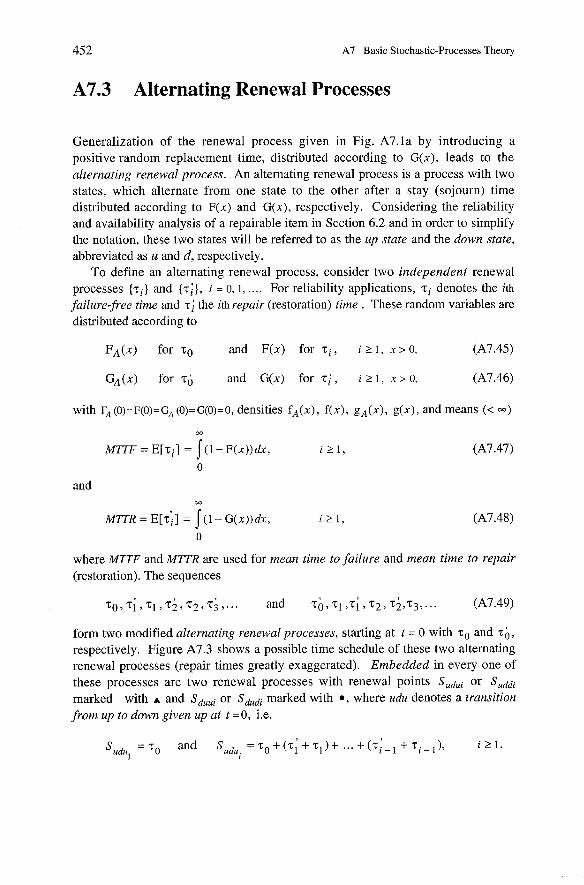
452 A7 Basic Stochastic-Processes Theory
A7.3 Alternating Renewal Processes
Generalization of the renewal process given in Fig. A7.la by introducing a positive random replacement time, distributed according to G(x), leads to the alternating renewal process. An alternating renewal process is a process with two states, which alternate from one state to the other after a stay (sojourn) time distributed according to F(x) and G(x), respectively. Considering the reliability and availability analysis of a repairable item in Section 6.2 and in order to simplify the notation, these two states will be referred to as the up state and the down state, abbreviated as u and d, respectively.
To define an alternating renewal process, consider two independent renewal processes { T ~ } and {T;), i = 0,1, .... For reliability applications, zi denotes the ith failure-free time and T ; the ith repair (restoration) time . These random variables are distributed according to
FA(x) for 70 and F(x) for z i , i t I , X > 0, (A7.45)
GA(x) for ~ , j and G(x) for T ; , i t 1, X > 0, (A7.46)
with F, (0)=F(O)=GA(O)=G(O)=O, densities fA(x), f(x), gA(x) , g(x), and means (< W)
M l T F = E[z i ] = J (1 - F(x))dx, i i l ,
0
and m
M U R = E[T;] = / ( I - G(x))&, i t l ,
0
where MTTF and MTTR are used for mean time to failure and mean time to repair (restoration). The sequences
form two modified alternating renewal processes, starting at t = 0 with zo and TS, respectively. Figure A7.3 shows a possible time schedule of these two alternating renewal processes (repair times greatly exaggerated). Embedded in every one of these processes are two renewal processes with renewal points Sudui or Suddi marked with A and Sduui or ,Ydudi marked with 0 , where udu denotes a transition from up to down given up at t = 0, i.e.
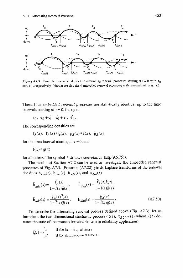
A7.3 Alternating Renewal Processes
Figure A7.3 Possible time schedule for two alternating renewal processes starting at t = 0 with 70 and 6, respectively (shown are also the 4 embedded renewal processes with renewal points . . A) These four embedded renewal processes are statistically identical up to the time intervals starting at t = 0, i.e. up to
The corresponding densities are
for the time interval starting at t = 0, and
f(x) * g(x)
for all others. The symbol * denotes convolution (Eq. (A6.75)). The results of Section A7.2 can be used to investigate the embedded renewal
processes of Fig. A7.3. Equation (A7.22) yields Laplace transforms of the renewal densities hudu(t), hduu(t), hudd(t), arid hdud(t)
huduW = fA ($1
Lduu(s) = ~ ( s )
1 - f (SI g(s) i - T(s)~(s) '
To describe the alternating renewal process defined above (Fig. A7.3), let us introduce the two-dimensional stochastic process ( <(t), z ~ ~ ( ~ )(t)) where <(t) de- notes the state of the process (repairable item in reliability application)
u if the item is up at time t
d if the item is down at time t
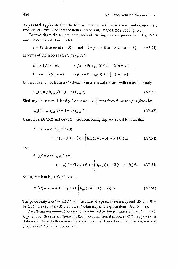
454 A7 Basic Stochastic-Processes Theory
~ , ~ ( t ) and ~ ~ ~ ( t ) are thus the fonvard recurrence times in the up and down states, respectively, provided that the item is up or down at the time t, See Fig. 6.3.
To investigate the general case, both alternating renewal processes of Fig. A7.3 must be combined. For this let
p = Pr{item up at t = 0) and 1 - p = Pr{item down at t = 0). (A7.51)
In tems of the process ( <(t) , T R (t ) ( t ) ) ,
Consecutive jumps from up to down form a renewal process with renewal density
Similarly, the renewal density for consecutive jumps from down to up is given by
Using Eqs. (A7.52) and (A7.53), and considering Eq. (A7.25), it follows that
t
= p ( 1 - F A ( t + 8 ) ) + ~ h d u ( ~ ) ( l - ~ ( t - x + 8 ) ) d x (A7.54) 0
and
Setting 8 = 0 in Eq. (A7.54) yields
The probability PA(t) = Pr(((t) = U} is called thepoint availability and IR(t,t + 81 =
Pr{<(t) = u n ~ ~ , ( t ) > 8) the intewal reliability of the given item (Section 6.2). An alternating renewal process, characterized by the Parameters p, FA(x), F(x),
G A ( x ) , and G(x) is stationary if the two-dimensional process ( ( ( t ) , ~ , < ~ ~ , ( t ) ) is stationary. As with the renewal process it can be shown that an alternating renewal process is stationary if and only if
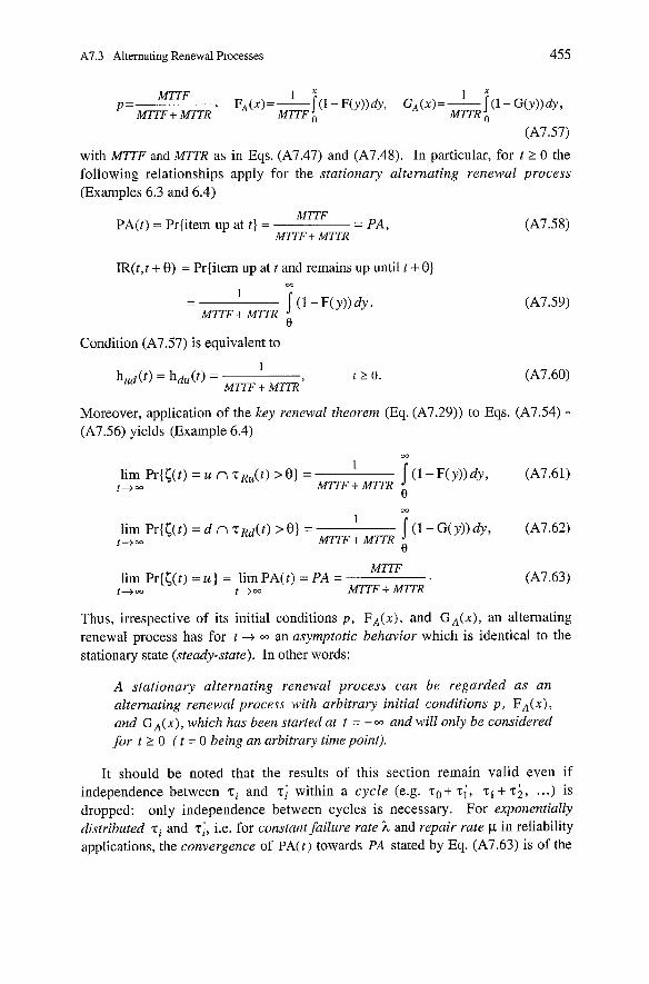
A7.3 Altemating Renewal Processes 455
(A7.57)
with MTTF and MTirR as in Eqs. (A7.47) and (A7.48). In particular, for t 2 0 the following relationships apply for the stationary alternating renewal process (Examples 6.3 and 6.4)
MTTF PA(t) = Pr{item up at t ] = = PA, (A7.58)
MTTF + MTTR
IR(t, t + 8 ) = Pr{item up at t and remains up until t + 81 Co ~ -
- - j ( l - ~ ( y ) ) d y . MTTF + MTTR
8
Condition (A7.57) is equivalent to
Moreover, application of the key renewal theorem (Eq. (A7.29)) to Eqs. (A7.54) - (A7.56) yields (Example 6.4)
lim Pr{c(t) = u n zRu(t) > 81 = t+m
1 - Y (A7.61) MTTF + MTTR e
lim Pr{<(t) = d n zRd( t ) > 8 ) = t+m
j ( l - G ( y ) ) d y , (-47.62) MTTF + MTTR
8
MTTF lim Pr{<(t) = u J = lim PA(t) = PA = (A7.63)
t-+- t+-= MTTF + MTTR
Thus, irrespective of its initial conditions p, FA(x) , and G A ( x ) , an alternating renewal process has for t -+ - an asymptotic behavior which is identical to the stationary state (steady-state). In other words:
A stationary alternating renewal process can be regarded as an alternating renewal process with arbitrary initial conditions p , FA(x), und G A ( x ) , which has been started at t = - W und will only be considered for t 2 0 ( t = 0 being an arbitrary time point).
It should be noted that the results of this section remain valid even if independence between z j and T; within a cycle (e.g. T O + T;, T~ + T;, ...) is dropped; only independence between cycles is necessary. For exponentially distributed z j and 21, i.e. for constant failure rate h and repair rate p in reliability applications, the convergence of PA(t) towards PA stated by Eq. (A7.63) is of the
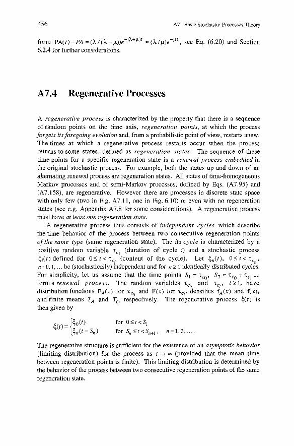
456 A7 Basic Stochastic-Processes Theory
form PA(t) -PA = (h 1 ( h + p))e-(h+p)t = (h ~ ~ ) e - ~ " See Eq. (6.20) and Section 6.2.4 for further considerations.
A7.4 Regenerative Processes
A regenerative process is characterized by the property that there is a sequence of random points on the time axis, regeneration points, at which the process forgets its foregoing evolution and, from a probabilistic point of view, restarts anew. The times at which a regenerative process restarts occur when the process returns to some states, defined as regeneration states. The sequence of these time points for a specific regeneration state is a renewal process embedded in the original stochastic process. For example, both the states up and down of an alternating renewal process are regeneration states. All states of time-homogeneous Markov processes and of serni-Markov processes, defined by Eqs. (A7.95) and (A7.158), are regenerative. However there are processes in discrete state space with only few (two in Fig. A7.11, one in Fig. 6.10) or even with no regeneration states (see e.g. Appendix A7.8 for some considerations). A regenerative process must have at least one regeneration state.
A regenerative process thus consists of independent cycles which describe the time behavior of the process between two consecutive regeneration points of the same type (same regeneration state). The ith cycle is characterized by a positive random variable zci (duration of cycle i) and a stochastic process t i ( t ) defined for 0 1 t < zCi (content of the cycle). Let t , ( t ) , 0 1: t < zcn, n= 0, I , ... be (stochastically) independent and for 12 2 i identically distributed cycles. For simplicity, let us assume that the time points SI = zcO, S2 = zco + ,... form a renewal process. The random variables zCo and T,, , i > 1, have distribution functions FA(x) for T , ~ and F(x) for T , ~ , densities f A ( x ) and f ( x ) , and finite means TA and T„ respectively. The regenerative process 5 ( t ) is then given by
The regenerative structure is sufficient for the existence of an asymptotic behavior (limiting distribution) for the process as t + (provided that the mean time between regeneration points is finite). This limiting distribution is determined by the behavior of the process between two consecutive regeneration points of the same regeneration state.
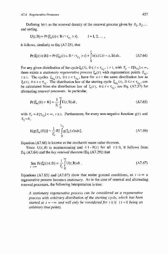
A7.4 Regenerative Processes 457
Defining h ( t ) as the renewal density of the renewal process given by S I , S 2 , ... and setting
it follows, similarly to Eq. (A7.25), that
For any given distribution of the cycle c i ( t ) , 0 5 t < zci, i 2 1, with Tc = E [ T , ~ ] < W,
there exists a stationary regenerative process c e ( t ) with regeneration points Sei, i 2 1. The cycles Ce, ( t ) , 0 5 t < have for n 2 1 the Same distribution law as c i ( t ) , 0 5 t < zCi. The distribution law of the starting cycle ce0 ( t ) , 0 5 t < T , ~ , can be calculated from the distribution law of & ( t ) , 0 5 t < T , ~ , See Eq. (A7.57) for alternating renewal processes. In particular,
with T, = E [ T , ~ ] < W , i 2 1. Furthermore, for every non-negative function g(t ) and S I =o ,
Equation (A7.66) is known as the stochastic mean value theorem. Since U(t , B) is nonincreasing and 5 1 - F(t) for all t 2 0, it follows from
Eq. (A7.64) and the key renewal theorem (Eq. (A7.29)) that
Equations (A7.65) and (A7.67) show that under general conditions, as t -+ 00 a regenerative process becomes stationary. As in the case of renewal and alternating renewal processes, the following interpretation is true:
A stationary regenerative process can be considered as a regenerative process with arbitrary distribution of the starting cycle, which has been started at t = - W und will only be consideved for t 2 0 ( t = 0 being an arbitrary time point).
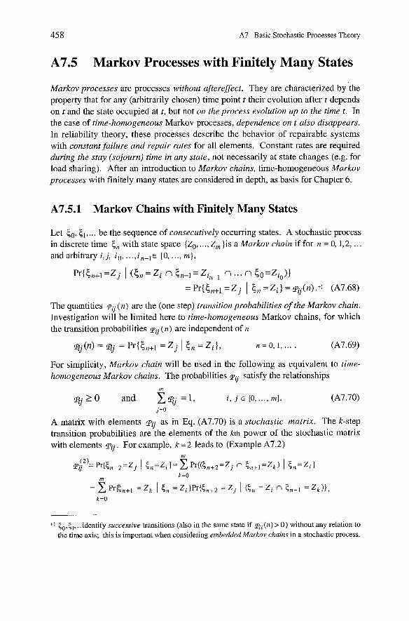
45 8 A7 Basic Stochastic-Processes Theory
A7.5 Markov Processes with Finitely Many States
Markov processes are processes without aftereffect. They are characterized by the property that for any (arbitrarily chosen) time point t their evolution after t depends on t and the state occupied at t , but not on the process evolution up to the time t. In the case of time-homogeneous Markov processes, dependence on t also disappears. In reliability theory, these processes describe the behavior of repairable Systems with constant failure und repair rates for all elements. Constant rates are required during the stay (sojourn) time in any state, not necessarily at state changes (e.g. for load sharing). After an introduction to Markov chains, time-homogeneous Markov processes with finitely many states are considered in depth, as basis for Chapter 6.
A7.5.1 Markov Chains with Finitely Many States
Let E,0, Ci ,. . . be the sequence of consecutively occurring states. A stochastic process in discrete time E,, with state space {Zo,. .., Z, }is a Markov chain if for n = 0, 1,2, .. . and arbitrary i, j, io , . . . , in-i E (0, . . . , m } ,
The quantities pv ( n ) are the (one step) transition probabilities of the Markov chain. Investigation will be limited here to time-homogeneous Markov chains, for which the transition probabilities pv ( n ) are independent of n
For simplicity, Markov chain will be used in the following as equivalent to time- homogeneous Markov chains. The probabilities pv satisfy the relationships
m
ej20 and xqj=l, i, j E {o, ... , m]. (A7.70) j=O
A matrix with elements pq as in Eq. (A7.70) is a stochastic matrix. The k-step transition probabilities are the elements of the kth power of the stochastic matrix with elements p ~ . For example, k = 2 leads to (Example A7.2)
m
Pr{5n+2=Zj I 5,=zi I = I-< P ~ { ( C , + ~ = Z ~ 5 n + 1 = Z k ) I 5,=zi I II m k=O
= = Zk 1 5, = Zi = Z j 1 (5, = Zi n 5„1 = Zk)l, k=O
50.5i,...identify successive transitions (also in the same state if pii(n) > 0 ) without any relation to the time axis; this is important when considering embedded Markov chains in a stochastic process.
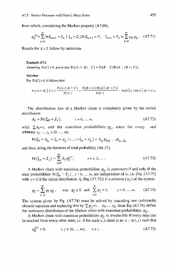
A7.5 Markov Processes with Finitely Many States 459
from which, considering the Markov property (A7.68),
Results for k > 2 follow by induction.
Example A7.2
Assuming Pr{C]>O,provethat Pr((A n B ) I C ] = Pr{B I C}Pr{A I ( B n C)]
Solution For Pr{C] 1 0 it follows that
The distribution law of a Markov chain is completely given by the initial distribution
Ai = P r { t O = Z i } , i = 0, ..., m, (A7.72)
with CAi=l, and the transition probabilities p ~ , since for every and arbitrary io, .... in E (0, . . ., m),
Pr{cO = Zi, n Ci = Zi, n ... n C,, = Z. In ) = A. 10 piOii ... pin-,in
and thus, using the theorem of total probability (A6.17),
A Markov chain with transition probabilities pg is stationary if and only if the state probabilities Pr{E,, = Zj J , j = 0, ... , m, are independent of n, i.e. (Eq. (A7.73) with n=1) if the initial distribution Ai (Eq. (A7.72)) is a solution (p j ) of the system
m m
, with p j 2 0 and z p j = l , j = O ,..., rn. (A7.74) i= 0 j=l
The system given by Eq. (A7.74) must be solved by canceling one (arbitrarily chosen) equation and replacing this by pj = 1. PO, . . . ,prn from Eq. (A7.74) define the stationary distribution of the Markov chain with transition probabilities TU.
A Markov chain with transition probabilities pg is irreducible if every state can be reached from every other state, i.e. if for each (i, j) there is an n = n(i, j) such that
(n ) Tg > O , i j { O m } , n t l . (A7.75)
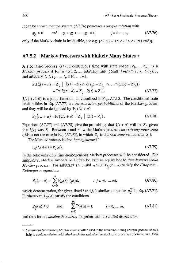
460 A7 Basic Stochastic-Processes Theory
It can be shown that the system (A7.74) possesses a unique solution with
p j > O and f i + % + . . . + p m = 1 , j = o , ..., m, (A7.7 6)
only if the Markov chain is irreducible, see e.g. [A7.3, A7.13, A7.27, A7.29 (1968)l.
A7.5.2 Markov Processes with Finitely Many States +I
A stochastic process <(t ) in continuous time with state space {Zo, . .., Z,} is a Markov process if for n= 0,1,2, ..., arbitrary time points t +U> t> tn> ... > to2 0 , and arbitrary i , j , iO , ..., in E {0, ..., m } ,
<( t ) ( t 2 0 ) is a jump function, as visualized in Fig. A7.10. The conditional state probabilities in Eq. (A7.77) are the transition probabilities of the Markov process and they will be designated by Pu ( t , t + U )
Equations (A7.77) and (A7.78) give the probability that <(t + U ) will be Zj given that <(t ) was Zi. Between t and t + a the Markov process can visit any other state (this is not the case in Eq. (A7.95), in which Zj is the next state visited after Zi).
The Markov process is time-homogeneous if
In the following only time-homogeneous Markov processes will be considered. For simplicity, Markov process will often be used as equivalent to time-homogeneous Markov process. For arbitrary t > 0 and a > 0 , Pij ( t + a ) satisfy the Chapman- Kolmogorov equations
k=O
which demonstration, for given fixed i and j, is similar to that for in Eq. (A7.71). Furthermore Pu ( U ) satisfy the conditions
and thus form a stochastic matrix. Together with the initial distribution
+) Continuous (parameter) Markov chain is often used in the literature. Using Markovprocess should help to avoid confusion with Markov chains embedded in stochastic processes (footnote onp. 458).
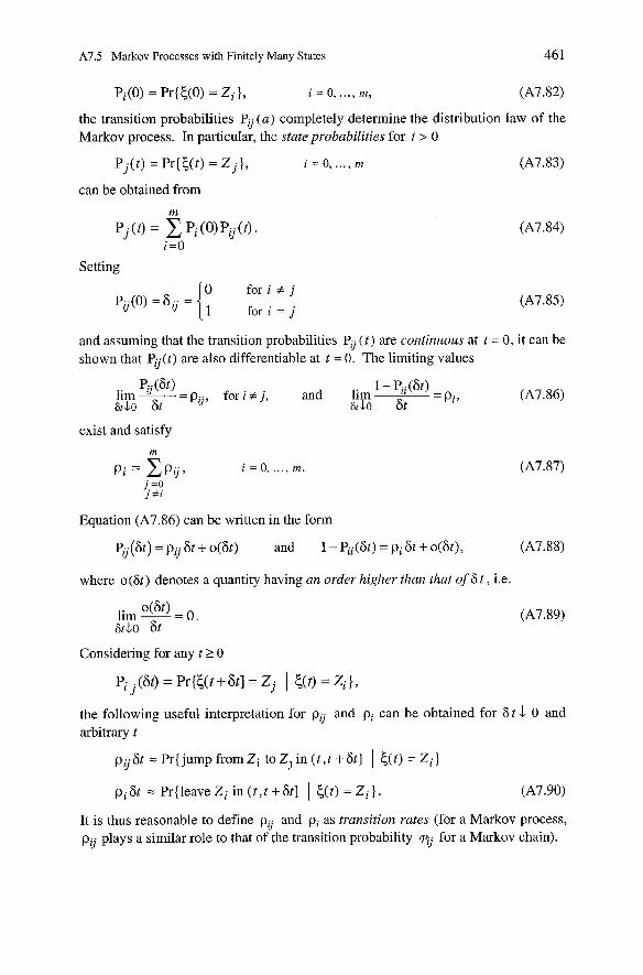
A7.5 Markov Processes with Finitely Many States 461
the transition probabilities Pij (U) completely determine the distribution law of the Markov process. In particular, the state probabilities for t > 0
Pj(t) = Pr{E,(t) = Z j}, i = 0, ..., m (A7.83)
can be obtained from
Setting
0 for i + j
and assurning that the transition probabilities Pij ( t ) are continuous at t = 0, it can be shown that Pij(t) are also differentiable at t = 0. The limiting values
P-(6t) 1 - Pii (Gt) l i m L = p„ for i 7~ j, and lim
6t.10 6t =Pi,
sr.10 6t
exist and satisfy
Equation (A7.86) can be written in the form
~ i j (6 t ) = p, 6t + o(6t) and 1 - Pii(&) = pi 6t + o(6t), (A7.8 8)
where o(6t) denotes a quantity having an order higher than that of 6 t , i.e.
Considering for any t 2 0
the following useful interpretation for pij and pi can be obtained for 6 t -1 0 and arbitrary t
pij 6t = Pr{ jump from Zi to Zj in (t , t t 6t] / &t) = Zi }
It is thus reasonable to define pij and pi as transition rates (for a Markov process, pij plays a sirnilar role to that of the transition probability pij for a Markov chain).
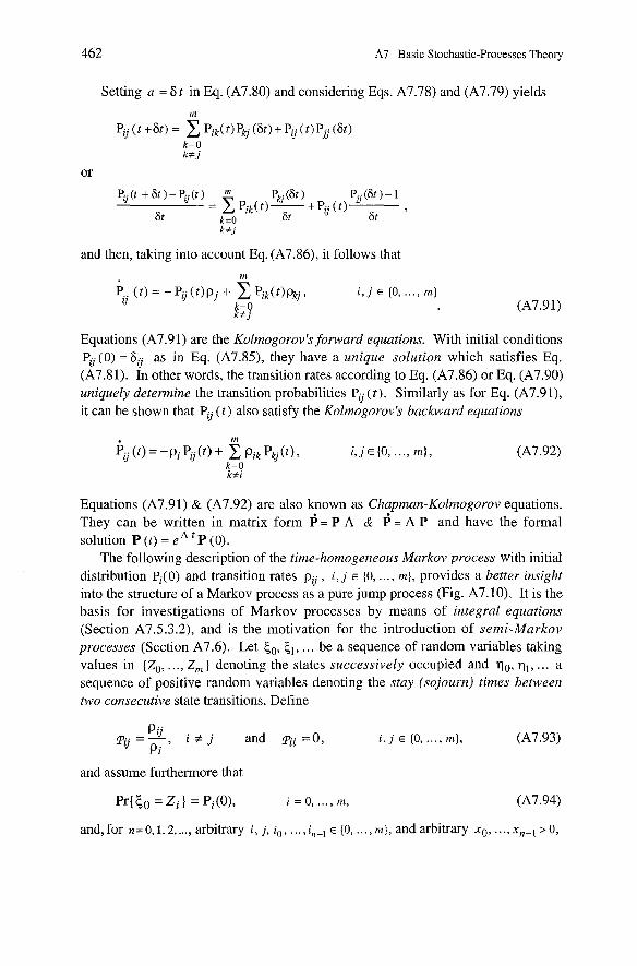
462 A7 Basic Stochastic-Processes Theory
Setting a = 6 t in Eq. (A7.80) and considering Eqs. A7.78) and (A7.79) yields
and then, taking into account Eq. (A7.86), it follows that
Equations (A7.91) are the Kolmogorov's fonvard equations. With initial conditions P,(O) = 6, as in Eq. (A7.85), they have a unique solution which satisfies Eq. (A7.81). In other words, the transition rates according to Eq. (A7.86) or Eq. (A7.90) uniquely determine the transition probabilities P, ( t ) . Similarly as for Eq. (A7.91), it can be shown that P, ( t ) also satisfy the Kolmogorov's backward equations
Equations (A7.91) & (A7.92) are also known as Chapman-Kolmogorov equations. They can be written in matrix form 6 = P A & 6 = A P and have the formal solution P ( t ) = e P (0).
The following description of the time-homogeneous Markov process with initial distribution Pi(()) and transition rates p,, i, j E (0, ..., m), provides a better insight into the structure of a Markov process as a pure jump process (Fig. A7.10). It is the basis for investigations of Markov processes by means of integral equations (Section A7.5.3.2), and is the motivation for the introduction of semi-Markov processes (Section A7.6). Let kO, Ci, . . . be a sequence of random variables taking values in {Zo, . .., Z, ) denoting the states successively occupied and qo, qi , . . . a sequence of positive random variables denoting the stay (sojourn) times between two consecutive state transitions. Define
Pij T U = ~ , i + j and pii = 0 , i , j E {O ,..., m ] , (A7.93)
and assume furthermore that
and, for n= O,1,2, ..., arbitrary i , j, io , ..., in-, E (0, .. . , m), and arbitrary xo, . .., x ~ - ~ > 0,
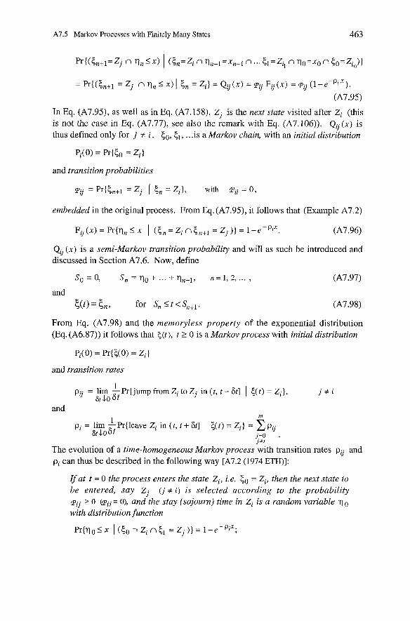
A7.5 Markov Processes with Finitely Many States 463
In Eq. (A7.93, as well as in Eq. (A7.158), Z j is the next state visited after Zi (this is not the case in Eq. (A7.77), see also the remark with Eq. (A7.106)). Q, (X) is thus defined only for j z i . Co, E I , . . .is a Markov chain, with an initial distribution
and transition probabilities
P, = Pr{kntl = Z j ( C,, = Zi} , with Pii = 0 ,
embedded in the original process. From Eq. (A7.93, it follows that (Example A7.2)
Qij (X) is a semi-Markov transition probability and will as such be introduced and discussed in Section A7.6. Now, define
So=O, S , = I I ~ + . . . + ~ ~ - ~ , n = 1 , 2 ,... ,
and E,(t) = E,„ for Sn 5 t <
From Eq. (A7.98) and the memoryless property of the exponential distribution (Eq. (A6.87)) it follows that 5(t), t 1 0 is a Markovprocess with initial distribution
Pi(0) = Pr{c(O) = Zi ]
and transition rates
1 p, = lim -Pr{jumpfromZitoZj in ( t , t+6t l I c ( t ) = Z i J , j + i
6rL0 6t and
1 m
pi = iim -Pr{leave Zi in ( t , t + 6t] I E,(t) = Zi} = p, i j tLoSt j,=o . ]?Li
The evolution of a time-homogeneous Markov process with transition rates p, and pi can thus be described in the following way [A7.2 (1974 ETH)]:
I f at t = 0 the process enters the state Zi , i.e. Co = Zi, then the next state to be entered, say Z j ( j # i ) is selected according to the probability pij 2 o (pii = O), and the stay (sojourn) time in Zi is a random variable with distribution function
-Pi". Pr{qo<x l (cO=~in\ l = Z i ) } = l - e ,
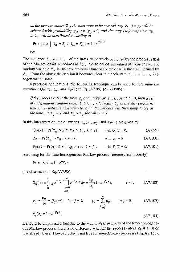
464 A7 Basic Stochastic-Processes Theory
as the process enters Z j , the next state to be entered, say Zk ( k + j), will be selected with probability qk 2 0 kpjj = 0) und the stay (sojourn) time q l in Z j will be distributed according to
etc.
The sequence C„ n = o, i , . . . of the states successively occupied by the process is that of the Markov chain embedded in C(t), the so called embedded Markov chain. The random variable q, is the stay (sojourn) time of the process in the state defined by C,,. From the above description it becomes clear that each state Zi , i = 0, ... , rn, is a regenerution state.
In practical applications, the following technique can be used to determine the quantities Qij ( X ) , pij , und Fij ( X ) in Eq. (A7.95) [A7.2 (1985)l:
Ifthe process enters the state Zi at an arbitravy time, say at t = 0, then a set of independent random times zij > 0, j it i, begin (zu is the stay (sojourn) time in Zi with the next jump to Z j ) ; the process will then jump to Z j at the time X i f 'tij = X und > zij for (all) k # j.
In this interpretation, the quantities Qij ( X ) , pij , and Fij (X) are given by
Qij(x) = Pr{zij 9 x n ~ i k > T V , k # j}, with Q,(O)= O , , (A7.99)
= Pr{zik > zij, k f j } , B with pii 3 0, (A7.100)
FU(x) = Pr{zij I x I Tik > ' tu, k # j } , with F,(O) = 0. (A7.101)
Assuming for the time-homogeneous Markov process (memoryless property)
one obtains, as in Eq. (A7.95),
m Pij P.. = - = Q . . (
II W ) for j i , p i = pij, P.. LI = O - > (A7.103) Pi i =O
It should be emphasized that due to the memoryless property of the time-homogene- ous Markov process, there is no difference whether the process enters Zi at t = 0 or it is already there. However, this is not true for semi-Markovprocesses (Eq. A7.158).
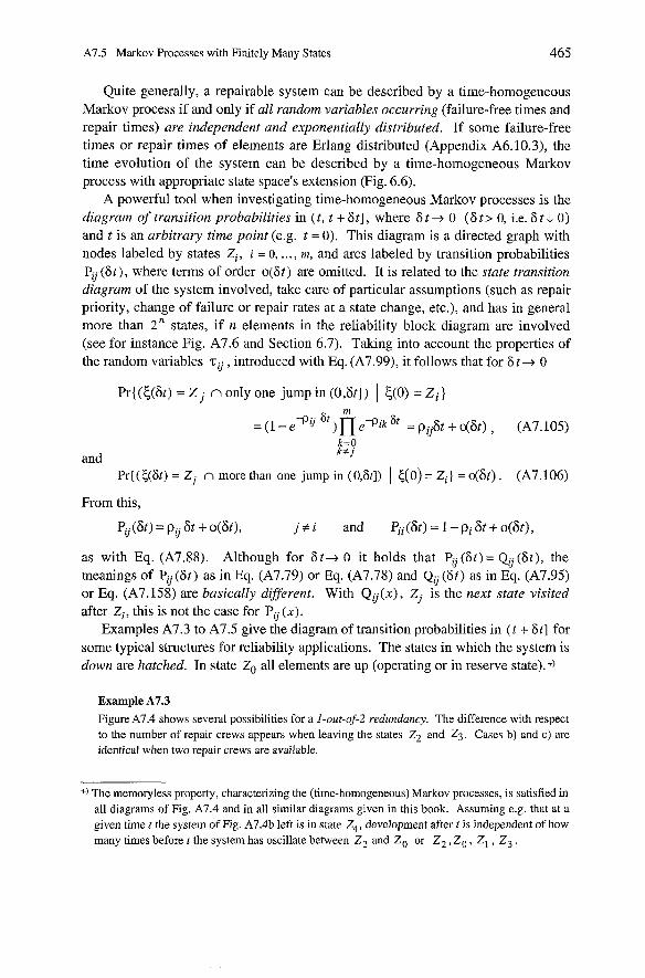
A7.5 Markov Processes with Finitely Many States 465
Quite generally, a repairable system can be described by a time-homogeneous Markov process if and only if all random variables occurring (failure-free times and repair times) are independent und exponentially distributed. If some failure-free times or repair times of elements are Erlang distributed (Appendix A6.10.3), the time evolution of the system can be described by a time-homogeneous Markov process with appropriate state space's extension (Fig. 6.6).
A powerful tool when investigating time-homogeneous Markov processes is the diagram of transition probabilities in (t , t + 6t], where 6 t -+ 0 (6 t:, 0, i.e. 6 t .1 0) and t is an arbitrary time point (e.g. t = 0). This diagram is a directed graph with nodes labeled by states Zi, i = 0, ... , rn, and arcs labeled by transition probabilities P, (6t), where terms of order o(6t) are omitted. It is related to the state transition diagram of the system involved, take care of particular assumptions (such as repair priority, change of failure or repair rates at a state change, etc.), and has in general more than 2" states, if n elements in the reliability block diagram are involved (see for instance Fig. A7.6 and Section 6.7). Taking into account the properties of the random variables T, , introduced with Eq. (A7.99), it follows that for 6 t + 0
Pr{(5(6t) = Z n only one jump in (0 ,6t] ) 1 k(0) = Zi )
and Pr{(E,(6t) = Zj n more than one jurnp in (OJt]) 1 c(0) = Zi) = o(6t). (A7.106)
From this,
P,(&) = p, 6t + o(6t), j + i and Pii (6t) = 1 - pi 6t + o(6t),
as with Eq. (A7.88). Although for 6 t + 0 it holds that P, (6t) = Q, (6t), the meanings of P, (6t) as in Eq. (A7.79) or Eq. (A7.78) and Q, (6t) as in Eq. (A7.95) or Eq. (A7.158) are basically dzjjferent. With Qij(x), Zj is the next state visited after Zi, this is not the case for P, (X).
Examples A7.3 to A7.5 give the diagram of transition probabilities in ( t + 6t] for some typical stmctures for reliability applications. The states in which the system is down are hatched. In state Zo all elements are up (operating or in reserve state). +)
Example A7.3 Figure A7.4 shows several possibilities for a 1-out-of-2 redundancy. The difference with respect to the number of repair crews appears when leaving the states Z2 and Z3. Cases b) and C) are identical when two repair crews are available.
+) The memoryless property, characterizing the (time-homogeneous) Markov processes, is satisfied in all diagrams of Fig. A7.4 and in all similar diagrams given in this book. Assuming e.g. that at a given time t the system of Fig. A7.4b left is in state Z4, development after t is independent of how many times before t the system has oscillate between Z2 and Zo or Z 2 , Zo , Z1 , Z3 .
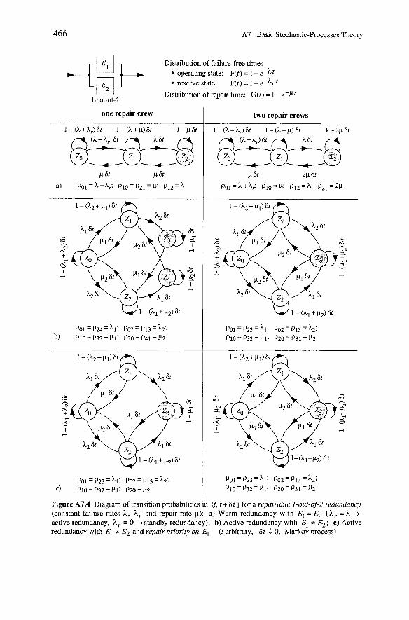
466 A7 Basic Stochastic-Processes Theory
Disiribution of failure-free times operating state: F(t) = 1 - ePht reserve state: F(t) = 1 - e-'r
Distribution of repair time: G(t) = 1 - e-Pt 1-out-of-2
one repair Crew two repair Crews
Figure A7.4 Diagram of transition probabilities in (t, t + 6 t ] for a repairable 1-out-of-2 redundancy (constant failure rates h, h , and repair rate P): a) Warm redundancy with El = E2 ( h , = h + active redundancy, h, = 0 jstandby redundancy); b) Active redundancy with EI * E2; C ) Active redundancy with EI # E2 and repairprion'ty on E1 ( t arbitrary, 6t .L 0, Markov process)
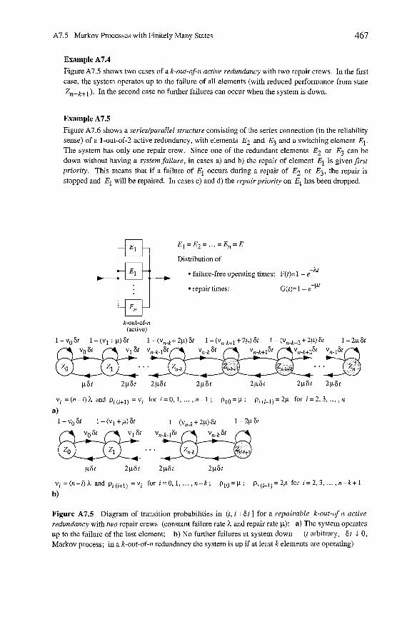
A7.5 Markov Processes with Finitely Many States
Example A7.4 Figure A7.5 shows two cases of a k-out-of-n active redundancy with two repair crews. In the first case, the system operates up to the failure of all elements (with reduced performance from state Zn-k+l). In the second case no further failures can occur when the system is down.
Example A7.5 Figure A7.6 shows a series/parallel structure consisting of the series connection (in the reliability sense) of a 1-out-of-2 active redundancy, with elements E2 and E3 and a switching element EI. The system has only one repair Crew. Since one of the redundant elements E2 or E3 can be down without having a system failure, in cases a) and b) the repair of element EI is givenfirst priority. This means that if a failure of E1 occurs during a repair of E2 or E3, the repair is stopped and El will be repaired. In cases C) and d) the repairpriority on E1 has been dropped.
E l = E 2 = ... = E n = E
Distribution of
failure-free operating times: F(t)=l - e -At
repair times: G(t)=l - e-Pr
k-out-of-n (active)
vi = (n-i) h and pi (i+l) = vi for i = 0, 1, ... , n- 1 ; p10 = p ; pi(i-l) = 2p for i = 2, 3, ... , n
vi =(n-i)A and pi(i+l) =vi for i=O,l , ..., n-k; p l O = p ; pi(i-l)=2p for i=2 ,3 , ..., n-k+l
b)
Figure A7.5 Diagram of transition probabilities in (t, t + 6t ] for a repairable k-out-of-n active redundancy with w o repair crews (constant failure rate h and repair rate P): a) The system operates up to the failure of ihe last element; b) No further failures at system down (t arbitrary, St .L 0, Markov process; in a k-out-of-n redundancy the system is up if at least k elements are operating)
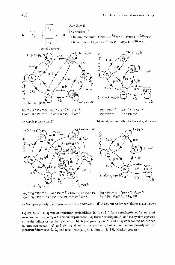
468 A7 Basic Stochastic-Processes Theory
E 2 = E 3 = E
Distribution of
failure-free times: F(t)= 1- e-L for E, F(+ 1- for E I
repair times: G(t)= 1- e-P for E , G(t)= 1- e-PIt for E1 U
1-out-of-2 (active)
a) Repair priority on E1 b) As a), but no further failures at syst. down
C) No repair priority (i.e. repair as per first-in first-out) d) As C), but no further failures at syst. down
Figure A7.6 Diagram of transition probabilities in (t, t + St] for a repairable series parallel structure with E2 = E3 = E and one repair crew: a) Repair priority on EI and the system operates up to the failure of the last element; b) Repair priority on EI and at system failure no further failures can occur; C) and d) as a) and b), respectively, but without repair priority on EI (constant failure rates h, hl and repair rates p, pl; t arbitrary; 6 t J 0, Markov process)
A7.5 Markov Processes with Finitely Many States 469
A7.5.3 State Probabilities and Stay Times (Sojourn Times) in a Given Class of States
In reliability theory, two important quantities are the state probabilities and the distribution function of the stay (sojourn) times in the set of system up states. The state probabilities allow calculation of the point availability. The reliability function can be obtained from the distribution function of the stay time in the set of system up states. Furthermore, a combination of these quantities allows for time- homogeneous Markov processes a simple calculation of the intewal reliability.
It is useful in such an analysis to subdivide the system state space into two complementary sets U and Ü
U = set of the system up states (up states at system level) - U = set of the system down states (down states at system level). (A7.107)
Partition of the state space in more than two classes is possible, see e.g. [A7.28]. Calculation of state probabilities and stay (sojourn) times can be carried out for
Markov processes using the method of differential equations or of integral equations.
A7.5.3.1 Method of Differential Equations
The method of dzfferential equations is the classical one used in investigating Markov processes. It is based on the diagram of transition probabilities in (t , t + 8t]. Consider a time-homogeneous Markov process c(t) with arbitrary initial distribution Pi(0) = Pr{c(O) = Zi} and transition rates p, and pi. The state probabilities defined by Eq. (A7.83)
Pj(t) = Pr{{(t) = Zj}, j = 0, ..., rn,
satisfy the system of differential equations
The proof of Eq. (A7.108) is sirnilar as for Eq. (A7.91), See also Example A7.6. The point availability PAs(t), for arbitrary initial conditions at t = 0, follows then from
PAS(t) = Pr{{(t) E U} = Pj(t). (A7.109) Z j € U
In reliability analysis, particular initial conditions are often of interest. Assurning
P i ( 0 ) = l and Pj(0)=O f o r j g i , (A7.110)
470 A7 Basic Stochastic-Processes Theory
i.e. that the system is in Zi at t = 0 (usually in state Zo denoting "all elements are up7'), the state probabilities Pj ( t ) are the transitionprobabilities Pv ( t ) defined by Eqs. (A7.78) & (A7.79) and can be obtained as
with Pj ( t ) as the solution of Eq. (A7.108) with initial conditions as in Eq. (A7.110), or of Eq. (A7.92). The point availability, now designated with PAs,(t), is then given by
PAsi(t) is the probability that the system is in one of the up states at t, given it was in Z, at t = 0 . Example A 7.6 illustrate calculation of the point-availability for a 1- out-of-2 active redundancy.
Example A7.6
Assume a I-out-of-2 uctive redunduncy, consisting of 2 identical elements EI = E2 = E with constant failure rate h and repair rate p, and only one repair Crew. Give the state probabilities of the involved Markov process ( EI and E2 are new at t = 0).
Solution
Figure A7.7 shows the diagram of transition probabilities in (t, t + St] for the investigation of the point availability. Because of the memoryless property of the involved Markov Process, Fig A7.7 and Eqs. (A7.83) & (A7.90) lead to (by omitting the terms in o(St), as per Eq. (A7.89))
and then, as St 0 ,
(t) = -(h + p) Pl ( t ) + 2 h Po (t) + p P, (t)
i2( t ) = -pP2(t) + h P, (t).
Equation (A7.113) also follows from Eq. (A7.108) with the p v from Fig. A7.7. The solution of Eq. (A7.113) with given initial conditions at t = 0 , e.g. Po(0) = 1, PI (0) = P2 (0) = 0 , leads to state probabilities Po(t), Pl(t), and P2(t), and then to the point availability according to Eqs. (A7.111) and (A7.112) with i = 0 (see also Example A7.9 and Table 6.2 for the solution).
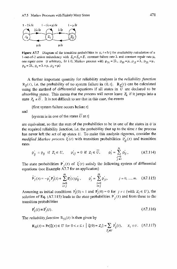
A7.5 Markov Processes with Finitely Many States
Figure A7.7 Diagram of the transition probabilities in (t, t + 6 t ] for availability calculation of a 1-out-of-2 active redundancy with E,=E,= E, constant failure rate h and constant repair rate p, one repair Crew (t arbitrary, 6 t .1 0, Markov process with pol = 2h, pI0 =p, pIZ = h, pZ1 = p , po=2h, p l = h + p 7 PZ=P)
A further important quantity for reliability analyses is the reliability function R s ( t ) , i.e. the probability of no system failure in (0, t ] . R s ( t ) can be calculated using the method of differential equations if all states in Ü are declared to be absorbing states. This means that the process will never leave Zk if it jumps into a state Zk E Ü. It is not difficult to See that in this case, the events
{first system failure occurs before t } and
{system is in one of the states Üat t }
are equivalent, so that the sum of the probabilities to be in one of the states in U is the required reliability function, i.e. the probability that up to the time t the process has never left the Set of up states U. To make this analysis rigorous, consider the rnodified Markov process ~ ' ( t ) with transition probabilities P~; ( t ) and transition
- pl. = pij if zi E U, p'.. = o if Z~ E U , p ) = C p i , II 11
(A7.114) j = O j jti
The state probabilities ~ ; . ( t ) of < ( t ) satisfy the following system of differential equations (see Example A7.7 for an application)
m m
$ ( t ) = -p;P;(t)+ z ~ / ( t ) ~ b , p: J = X p:., J Z j = 0, ..., m. (A7.115) i=O i= 0 i+ j i+ j
Assuming as initial conditions P:(o) = 1 and P;.(o) = 0 for j + i (with Zi E U), the solution of Eq. (A7.115) leads to the state probabilities P ; ( t ) and from these to the transition probabilities
P; ( t ) = P; ( t ) . (A7.116)
The reliabilityfinction Rsi( t ) is then given by
Rsi(t) = Pr{<(x) E U for 0 < X < t 1 <(o) = zi) = X ~ : j ( t ) , Z , e U . (A7.117) zj €U
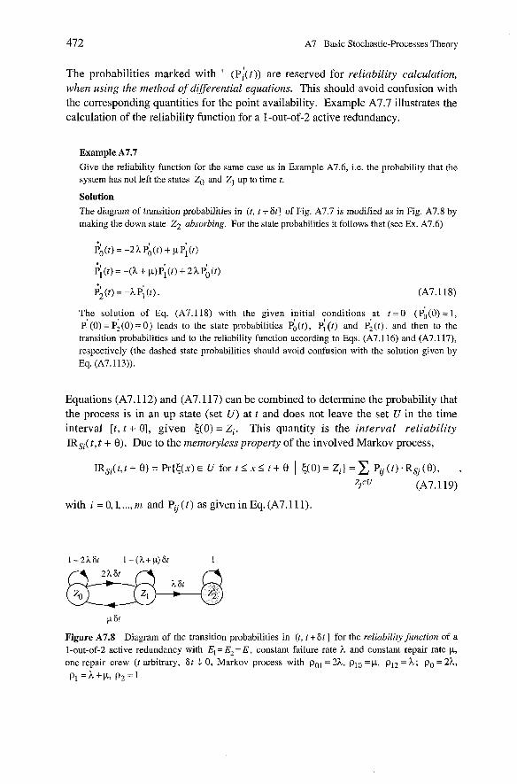
472 A7 Basic Stochastic-Processes Theory
The probabilities marked with ' ( ~ i ( t ) ) are reserved for reliability calculation, when using the method of differential equations. This should avoid confusion with the corresponding quantities for the point availability. Example A7.7 illustrates the calculation of the reliability function for a 1-out-of-2 active redundancy.
Example A7.7 Give the reliability function for the same case as in Example A7.6, i.e. the probability that the system has not left the states ZO and Z1 up to time t.
Solution The diagram of transition probabilities in (t, t +6t] of Fig. A7.7 is modified as in Fig. A7.8 by making the down state Z2 absorbing. For the state probabilities it follows that (see Ex. A7.6)
62 (t) = -h P; (t) . (A7.118)
The so1u;ion of Eq. (A7.118) with the given iritial tonditions ,at t=O ( ~ ' ~ ( 0 ) = 1 , PI (0) = P2(0) = 0 ) leads to the state probabilities P,,(t), P, (t) and P2(t), and then to the transition probabilities and to the reliability function according to Eqs. (A7.116) and (A7.117), respectively (the dashed state probabilities should avoid confusion with the solution given by Eq. (A7.113)).
Equations (A7.112) and (A7.117) can be combined to determine the probability that the process is in an up state (set U) at t and does not leave the set U in the time interval [t , t + B], given { (0 ) = Zi. This quantity is the interval reliability IRsi(t, t + 0). Due to the memoryless property of the involved Markov process,
IRsi(t,t + 0) = Pr(&x) E U for t 5 x < t + B 1 { ( O ) = Zi} = P, ( t ) .Rsj (B) , , zjcu (A7.119)
with i = 0,1, ..., m and Pu ( t ) as given in Eq. (A7.111).
Figure A7.8 Diagram of the transition probabilities in (t, t + 6t] for the reliabilityfunction of a 1-out-of-2 active redundancy with E,= E2=Ei constant failure rate h and constant repair rate y, one repair Crew (t arbitrary, 6t 0, Markov process with pol = 2h, pm = y, p12 = h ; p, = 2h, P1 = h + y , P 2 = 1
A7.5 Markov Processes with Finitely Many States 473
A7.5.3.2 Method of Integral Equations
The method of integral equations is based on the representation of the (time-homo- geneous) Markov process g(t) as a pure jump process by means of 5, and q , as intro- duced in Appendix A7.5.2 (Eq. (A7.95), Fig. A7.10). From the mernoryless property it uses only the fact that jump points (in a new state) are regeneration points of g(t).
The transition probabilities Pij ( t ) = Pr{g(t) = Zj 1 &0) = Zi} can be obtained by solving the following system of integral equations
with pi=Xjsjti P, , 6,=O for j+i, &=I. To prove Eq. (A7.120), consider that
Pij(t) = Pr{(k(t) = Z n no jumps in (0, t ] ) 1 4(O) = Zi ) m
+ Pr{(t(t) = Zj n firstjump in (0, t] in Zk) 1 e(0) = Zi] k=O k+i
The first term of Eq. (A7.121) only holds for j = i and gives the probability that the process will not leave the state Zi (e-P" = P ~ { z ~ > t for all j + i ] according to the interpretation given by Eqs. (A7.99) - (A7.104)). The second term holds for any j ;t i , it gives the probability that the process will move first from Zi to Zk and take into account that the occurrence of Zk is a regeneration point. Accord- ing to Eq. (A7.95), Pr { = Zk n qo < X 1 g(0) = Zi} = Qik(x) = pik(l -CPix) and Pr{<(t) = Zj 1 ( C 0 = Zi n qo = X n Ci = Zk)} = Gj ( t - X ) . Equation (A7.120) then follows from the theorem of total probability (Eq. (A6.17)).
In the Same way as for Eq. (A.121), it can be shown that the reliabilityfunction RS i ( t ) , as defined in Eq. (A7.117), satisfies the following system of integral equations
Point availability PASi(t) and IRsi(t, t + 8) are given by Eqs. (A7.112) & (A7.119), with Pij(t) per Eq. (A7.120). The use of integral equations for PASi(t) can lead to mistakes, since RSi(t) and PASi(t) describe two different situations (summing for PASi(t) over all states j E (0, ... , m} leads to PASi( t )=l) .
474 A7 Basic Stochastic-Processes Theory
The Systems of integral equations (A7.120) and (A7.122) can be solved using Laplace transforms. Referring to Appendix A9.7,
and
A direct advantage of the method based on integral equations appears in the calculation of the mean stay (sojourn) time in the up states. Denoting by MTTQ the system mean time to failure, provided the system is in state Zi E U at t = 0, it follows that (Eq. (A6.38), Appendix A9.7)
D0
M T T F ~ ~ = J ~ ~ ~ ( t ) d t = KSi(o). (A7.125) 0
Thus, according to Eq. (A7.124), MTTFSi satisfies the following system of algebraic equations (see Example A7.9 an application)
1 P .. m
M 7 q i = - + ~ m j , Pi=xP„ Z i € U . (A7.126) Pi zjEupi j=o
j t i j #i
A7.5.3.3 Stationary State and Asymptotic Behavior
The determination of time-dependent state probabilities or of the point availability of a system whose elements have constant failure and repair rates is still possible using differential or integral equations. However, it can become time-consuming. The situation is easier where the state probabilities are independent of time, i.e. when the process involved is stationary (the system of differential or integral equations reduces to a system of algebraic equations):
A time-homogeneous Markov process <( t ) with states ZO, . . ., Zm is stationary, ifits state probabilities Pi(t) = Pr{<(t) = Zi } , i = 0, ... , rn do not depend on t.
This can be Seen from the following relationship
Pr{k(tl) = Zi n ... n 5(tn) = Zin } = PrIS(ti) = Zil IPili2 ( t 2 - t l )... Pi,-li, (tn - tn-l
which, according to the Markov property (Eq. (A7.77)) must be valid for arbitrary tl < ... C t , and i, , ... , in E {O, ... , m). For any a > 0 this leads to
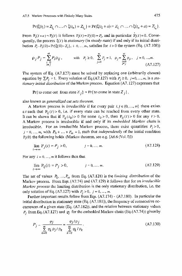
A7.5 Markov Processes with Finitely Many States 475
From Pi(t + U ) = Pi(t) it follows Pi(t) = Pi(0) = 4, and in particular Pi(t)=O. Conse- quently, the process c ( t ) is stationary (in steady-state) if and only if its initial distri- bution q=Pi(0)=Pr{~(O)=Zi] , i=O, ... , m , satisfies for t > 0 the system (Eq. (A7.108))
m m m
P J . P . J = E p i p i j , with P j T O , Z p j = l , p . = Z p . . , J 11 j = O ,..., rn. i=O j=O i=O i+ j i * j (A7.127)
The system of Eq. (A7.127) must be solved by replacing one (arbitrarily chosen) equation by x P j = 1. Every solution of Eq.(A7.127) with Pj 2 0 , j =O, . . . , rn, is a sta- tionary initial distribution of the Markov process. Equation (A7.127) expresses that
Pr{ to come out from state Z J = Pr{ to come in state Z } ,
also known as generalized cut sets theorem. A Markov process is irreducible if for every pair i, j E {0, ..., in} there exists
a t such that P, ( t ) > 0 , i.e. if every state can be reached from every other state. It can be shown that if P, ( t o ) > 0 for some to > 0 , then P, ( t ) > 0 for any t > 0. A Markov process is irreducible if and only if its embedded Markov chain is irreducible. For an irreducible Markov process, there exist quantities q >O, j = 0, . . . , rn, with Po + . . . + Pm = 1, such that independently of the initial condition Pi(0) the following holds (Markov theorem, See e.g. [A6.6 (Vol. I)])
lim Pj(t) = P j > 0 , j = o , ..., m. (A7.128) t - fm
For any i = 0, ... , m it follows then that
lim Pij( t ) = P j >O, j = 0, ..., m. t - f W
The set of values Po, ..., Pm from Eq. (A7.128) is the limiting distribution of the Markov process. From Eqs. (A7.74) and (A7.129) it follows that for an irreducible Markov process the limiting distribution is the only stationary distribution, i.e. the only solution of Eq. (A7.127) with q > 0 , j = 0 , ... , m.
Further important results follow from Eqs. (A7.174) - (A7.180). In particular the initial distribution in stationary state (Eq. (A7.18 I)), the frequency of consecutive oc- currences of a given state (Eq. (A7.182)), and the relation between stationary values Pj from Eq. (A7.127) and 1;. for the embedded Markov chain (Eq.(A7.74)) givenby
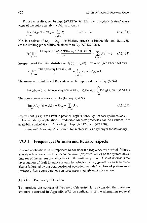
476 A7 Basic Stochastic-Processes Theory
From the results given by Eqs. (A7.127)-(A7.129), the asymptotic & steady-state value of the point availability PAs is given by
If K is a subset of {Zo, ..., Zm), the Markov process is irreducible, and Po, ..., Pm are the limiting probabilities obtained from Eq. (A7.127) then,
total sojourn time in states Z j E Kin (0, t] Pr{ lim = P j ) = 1 (A7.132)
t+m t Z j € K
irrespective of the initial distribution Po(0), ..., Pm(0). From Eq. (A7.132) it follows
total operating time in (0,tl = C = PAS = Pr{ lim
t+m t Z j € U
The average availability of the system can be expressed as (see Eq. (6.24)) t
1 AAs(t) =- E[total operating time in (0, t] 1 c(0) =Zi] = PA%(^) dr . (A7.133)
t t 0
The above considerations lead to (for any Zi E U )
Expressions kPk are useful in practical applications, e.g. for cost optimizations. For reliability applications, irreducible Markov processes can be assumed, for
availability calculations. According to Eqs. (A7.127) and (A7.128),
asymptotic & steady-state is used, for such cases, as a synonym for stationary.
A7.5.4 Frequency / Duration and Reward Aspects
In some applications, it is important to consider the frequency with which failures at system level occur and the mean duration (expected value) of the system down time (or of the system operating time) in the stationary state. Also of interest is the investigation of fault tolerant Systems for which a reconfiguration can take place after a failure, allowing continuation of operation with defined loss of performance (reward). Basic considerations on these aspects are given in this section.
A7.5.4.1 Frequency / Duration
To introduce the concept of frequency /duration let us consider the one-item structure discussed in Appendix A7.3 as application of the alternating renewal
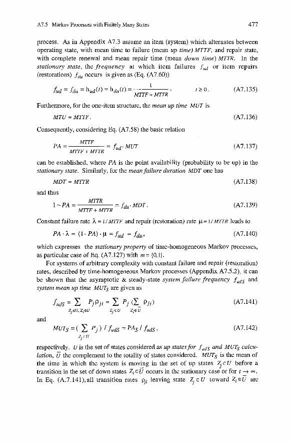
A7.5 Markov Processes with Finitely Many States 477
process. As in Appendix A7.3 assume an item (system) which alternates between operating state, with mean time to failure (mean up time) MTTF, and repair state, with complete renewal and mean repair time (mean down time) MTTR. In the stationary state, the frequency at which item failures fud or item repairs (restorations) fdu occurs is given as (Eq. (A7.60))
Furthermore, for the one-item structure, the mean up time MUT is
MTU = MTTF. (A7.136)
Consequently, considering Eq. (A7.58) the basic relation
MTTF PA = = fud + MUT (A7.137)
MTTF + MTTR
can be established, where PA is the point availability (probability to be up) in the stationary state. Similarly, for the mean failure duration MDT one has
MDT = MTTR (A7.138)
and thus MTTR
1-PA= = fdu. MDT. (A7.139) MTTF + MTTR
Constant failure rate ?L = I I MTTF and repair (restoration) rate p = I /MT772 leads to
which expresses the stationary property of time-homogeneous Markov processes, as particular case of Eq. (A7.127) with rn = (0,l).
For Systems of arbitrary complexity with constant failure and repair (restoration) rates, described by time-homogeneous Markov processes (Appendix A7.5.2), it can be shown that the asymptotic & steady-state System fuilure frequency fudS and system mean up time MUTs are given as
respectively. U is the set of states considered as up states for fudS und MUTs calcu- lation, 6 the complement to the totality of states considered. MUTS is the mean of the time in which the system is moving in the set of up states $ E U before a transition in the set of down states Zi EÜ occurs in the stationary case or for t + -. In Eq. (A.7.141),all transition rates pji leaving state 5 E U toward Zi EÜ are
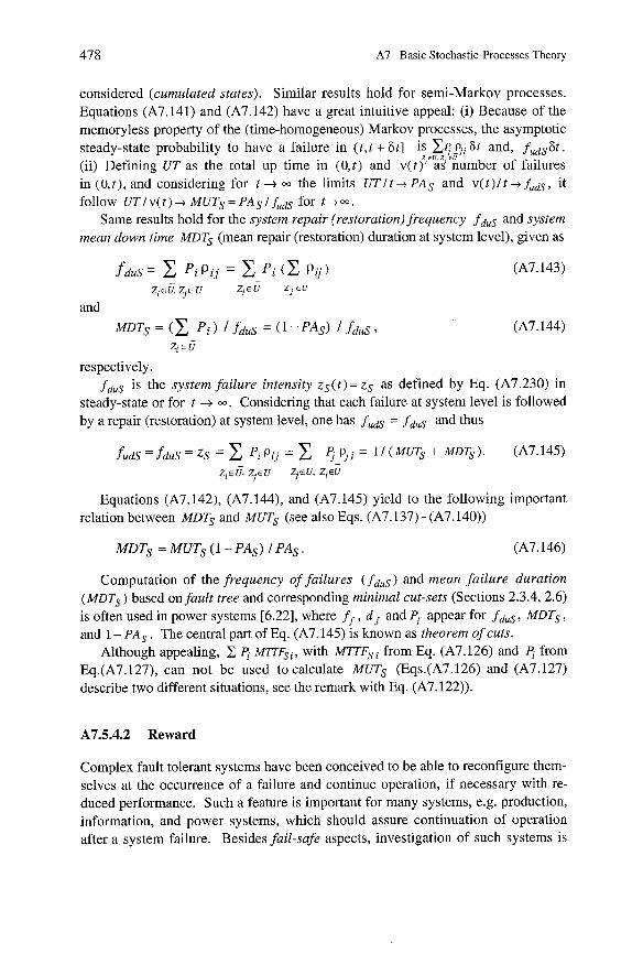
478 A7 Basic Stochastic-Processes Theory
considered (curnulated states). Similar results hold for semi-Markov processes. Equations (A7.141) and (A7.142) have a great intuitive appeal: (i) Because of the memoryless property of the (time-homogeneous) Markov processes, the asymptotic steady-state probability to have a failure in ( t , t + 8t] i ;s%s~i fit and, fuds&t. (ii) Defining UT as the total up time in (0 , t ) and v( t ) ' aS number of failures in (0, t ) , and considering for t + the limits UTI t i, PAS and v ( t ) l t + fudS, it f0110~ U T / v ( t ) + MUTS=PASl fuds f0r t+m.
Same results hold for the system repair (restoration) frequency fduS and System mean down time MDTs (mean repair (restoration) duration at system level), given as
and
MDTs = ( E Pi fdus = (1 - PAS) fdus , (A7.144) zi € 6
respectively. fduS is the system failure intensity z s ( t ) = z s as defined by Eq. (A7.230) in
steady-state or for t + W . Considering that each failure at system level is followed by a repair (restoration) at system level, one has fudS = fduS and thus
Equations (A7.142), (A7. I@), and (A7.145) yield to the following important relation between MDTs and MUTs (see also Eqs. (A7.137) - (A7.140))
Computation of the frequency of failures ( fduS) and mean failure duration (MDTs ) based on fault tree and corresponding minimal cut-sets (Sections 2.3.4, 2.6) is often used in power systems [6.22], where f f , df and Pf appear for fduS, MDTS, and 1 - PAs . The central part of Eq. (A7.145) is known as theorem of cuts.
Although appealing, C 4 MITFSi, with M= from Eq. (A7.126) and 8 from Eq.(A7.127), can not be used to calculate MUTS (Eqs.(A7.126) and (A7.127) describe two different situations, see the remark with Eq. (A7.122)).
A7.5.4.2 Reward
Complex fault tolerant systems have been conceived to be able to reconfigure them- selves at the occurrence of a failure and continue operation, if necessary with re- duced performance. Such a feature is important for many systems, e.g. production, information, and power systems, which should assure continuation of operation after a system failure. Besides fail-safe aspects, investigation of such systems is
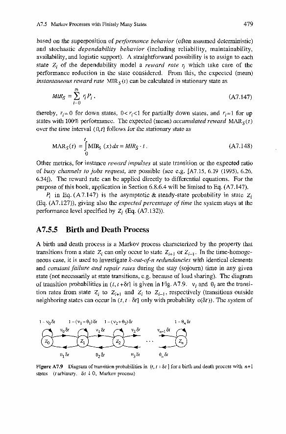
A7.5 Markov Processes with Finitely Many States 479
based on the superposition of pe$ormance behavior (often assumed deterministic) and stochastic dependability behavior (including reliability, maintainability, availability, and logistic support). A straightfonvard possibility is to assign to each state Zi of the dependability model a reward rate 5 which take care of the performance reduction in the state considered. From this, the expected (mean) instantaneous reward rate MIRs ( t ) can be calculated in stationary state as
thereby, ri= 0 for down states, 0< ri<l for partially down states, and ri=l for up states with 100% performance. The expected (mean) accumulated reward MARS(t) over the time interval (0, t] follows for the stationary state as
Other metrics, for instance reward impulses at state transition or the expected ratio of busy channels to jobs request, are possible (see e.g. rA7.15, 6.19 (1995), 6.26, 6.341). The reward rate can be applied directly to differential equations. For the purpose of this book, application in Section 6.8.6.4 will be limited to Eq. (A7.147).
< in Eq. (A7.147) is the asymptotic & steady-state probability in state Zi (Eq. (A7.127)), giving also the expected percentage of time the system stays at the performance level specified by Zi (Eq. (A7.132)).
A7.5.5 Birth and Death Process
A birth and death process is a Markov process characterized by the property that transitions from a state Zi can only occur to state Zi+l or ZiFl . In the time-homoge- neous case, it is used to investigate k-out-ofn redundancies with identical elements and constant failure und repair rates during the stay (sojourn) time in any given state (not necessarily at state transitions, e.g. because of load sharing). The diagram of transition probabilities in ( t , t +6t] is given in Fig. A7.9. vi and Bi are the transi- tion rates from state S i to Zi+l and Zi to Zi-l, respectively (transitions outside neighboring states can occur in ( t , t +6t] only with probability o(6t)). The system of
Figure A7.9 Diagram of transition probabilities in (t, t + 6t ] for a birth and death process with n + l states (t arbitrary, 6 t L 0, Markov process)
480 A7 Basic Stochastic-Processes Theory
differential equations describing the birth und death process given in Fig. A7.9 is
P j ( t ) = - ( v j + O j ) P j ( t ) + vj-I P jp i ( t ) + Oj+i Pj+,(t)
with Oo = V-i = V n = = 0, j= 0, ..., n . (A7.149)
The conditions v j > 0 ( j = 0, ... , n - 1 ) and Oj
for the existence of the limiting probabilities
lim Pj ( t ) = P' , with Pj > 0 t - fw
> 0 ( j = 1 , ... , n < 00) are sufficient
n
and ~ P J . = 1. (A7.150) j=O
It can be shown (Example A7.8), that the probabilities PJ , j = 0, ... , n are given by
n V. .. . Vi-1 P. = n . p = n j / Z n i , with n i = and no=l . (A7.151)
J J 0 i=O 0, ... 0,
From Eq. (A7.151) one recognizes that
P k ~ k =Pk+l@k+l? (k = 0, ..., n-1).
this holds quite general for time-homogeneous Markov processes (Eq. (A7.127)).
Example A7.8
Assuming Eq. (A7.150) prove Eq. (A7.151).
Solution
Considering Eqs. (A7.149) & (A7.150), P' are the solution of following system of algebraic eqs.
0 = -voPo + OiP1
0 = -OnPn + v ~ - ~ P , - ~ .
From the first equation it follows P, = Gvo 10,. With this 4 , the second equation leads to
Recursively one obtains
Considering Po + ... f P, = 1, Po follows and thenEq. (A7.151).
The values of Pj given by Eq. (A7.15 1) can be used in Eq. (A7.134) to calculate the stationary (asymptotic & steady-state) value of the point availability. The system mean time to failure follows from Eq. (A7.126). Examples A7.9 and A7.10 are applications of the birth and death process.
A7.5 Markov Processes with Finitely Many States
Example A7.9 For the 1-out-of-2 active redundancy with one repair Crew of Examples A7.6 and A7.7, i.e. for - vo = 2 h , v1 = h , O1 = O2 = p, U = { Z O , Z 1 ) and U = { Z 2 ), give the asymptotic & steady- state value PAS of the point availability and the mean time to failure M7TFS0 and M7TFsl.
Solution The asymptotic & steady-state value of point availability is given by Eqs. (A7.134) and (A7.151)
1 t 2 h / p p2 + 2 h p PA, = Po t P, = -
1 + 2 h l p + 2 h 2 / p 2 2 h ( h + p ) + p 2
The system's mean time to failure follows from Eq. (A7.126) with pol=p0 =2h , p12 = h , Pio=P. ~ l = h + ~ ,
M7TFso = 1 / 2 h + M-
1 P MnFs, = + - MVFs ,
h t p h + p
yielding 3 1 + p 2 h + p
MTTFso = - and MITFsl = - 2 h2 2 a2
Example A7.10
A computer system consists of 3 identical CPUs. Jobs arrive independently and the arrival times form a Poisson process with intensity h . The duration of each individual job is distributed exponentially with parameter p. All jobs have the same memory requirements D. Give for h = 2 p the minimum size n of the memory required in units of D, so that in the stationary case (asymptotic & steady-state) a new job can immediately find Storage space with a probability y of at least 95%. When ovefflow occurs, jobs are queued.
Solution
The problem can be solved using the following birth and death process
1 - h 6 t 1 - ( h + p ) 6 r 1 - ( h + 2 p ) 6 t 1 - ( h + 3 p ) & 1 - (h+3p)Ot
h 6 t h 6 t
... ...
P 6t 2 p 6t 3pS t 3p6t 3 p 6t 3 ~ 6t
In state Zi , exactly i memory units are occupied. n is the smallest integer such that in the steady- state, Po + ... t P,-1 = y 2 0.95 (if the assumption were made that jobs are lost if ovefflow occurs, then the process would stop at state Z n ) . For steady-state, Eq. (A7.127) yields
O=-hPo+pFj O = h P o - ( h + p ) e + 2 p P 2 O = h e - ( k + 2 p ) P 2 +3pP3 O = h P 2 - ( h + 3 p ) q +3pP4
482 A7 Basic Stochastic-Processes Theory
The solution leads to
n Assuming lim C = 1 and considering - < 1 it follows that
n-+- i=o 3
h " 9 h l p . h 3 ( ~ l p ) ~ Po[I+-+ -(-)"=p,[l+-+ I = 1 ,
P j=2 2 3 2 ( 3 - h l p )
from which
The size of the memory n can now be detennined from
2 ( 3 - A l p ) "-1 9 h l p U+-+ C, - ( - ) ] > Y .
6 + 4 h / ~ + ( h / p ) ~ i=2
For h 1 P = 2 and y = 0.95, the smallest n satisfying the above equation is n = 9 ( Po = 11 9,
P, = 2 / 9 , q =2i-113i f o r i t 2 ) .
As shown by Examples A7.9 and A7.10, reliability applications of birth and death processes identify v i as failure rates and Bi as repair rates. In this case,
v j < < Q j + l , j = 0 , ..., n - 1 ,
with v j and O j as in Fig. A7.9. Assuming 0 < r < 1 and thus
the following relationships for the steady-state probability Pj can be obtained (Example A7.11)
P. > . Pi, O < r < i , j , , - 1 , n > j . (A7.156) ' - r(1-rn- ') i=j+l
For r 5 11 2 it follows that
n
Equation (A7.157) states that for 2 v j .I Bj the steady-state probability in a state Z j of a birth and death process described by Fig. A7.9 is 2 the sum of the steady- state probabilities in all states following Zj , j = 0 , ..., n - i [2.50 (1992)l. This relationship is useful in developing approximate expressions for system availability.
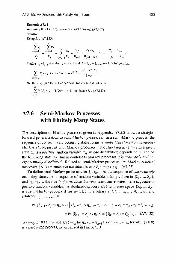
A7.5 Markov Processes with Finitely Many States
Example A7.11 Assuming Eq.(A7.155), prove Eqs. (A7.156) and (A7.157).
Solution Using Eq. (A7.150),
Setting S r for O < r < l and i = j , j+1, ..., n-1,itfollowsthat
and thus Eq. (A7.156). Furthermore, for r 5 11 2 it holds that n
I Pj S 1 - (11 2)n-j 5 1, and hence Eq. (A7.157). i=j+l
A7.6 Semi-Markov Processes with Finitely Many States
The description of Markov processes given in Appendix A7.5.2 allows a straight- forward generalization to semi-Markov processes. In a semi-Markov process, the sequence of consecutively occurring states forms an embedded (time-homogeneous) Markov chain, just as with Markov processes. The stay (sojourn) time in a given state Zi is a positive random variable zu whose distribution depends on Zi and on the following state Z j , but in contrast to Markov processes it is arbitrarily und not exponentially distributed. Related to semi-Markov processes are Markov renewal processes ( ~ ~ ( t ) = number of transitions in state Zi during (0,tl) [A7.23].
To define semi-Markov processes, let kO, Ci , . . . be the sequence of consecutively occurring states, i.e. a sequence of random variables taking values in {ZO, ..., Z m ] , and qo , q l , ... the stay (sojourn) times between consecutive states, i.e. a sequence of positive random variables. A stochastic process c ( t ) with state space {Zo, . . ., Zm ) is a semi-Markov process if for n= 0,1,2, ..., arbitrary i , j , io , ..., in-, E (0, ... , m), and arbitrary xo, .. ., x,-~ > 0 ,
E,(t)=& for 0 1 t< q o and t ( t ) =4, for q o +... t qn - l I t < qo+ ... + q n for n2 1 ( t 2 0) is a pure jump process, as visualized in Fig. A7.10.
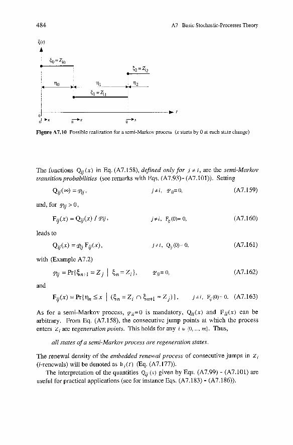
A7 Basic Stochastic-Processes Theory
o*" oux oux
Figure A7.10 Possible realization for a semi-Markov process (X starts by 0 at each state change)
The functions Qij ( X ) in Eq. (A7.158), defined only for j + i , are the semi-Markov transition probabilities (see remarks with Eqs. (A7.93) - (A7.101)). Setting
and, for pij ,J 0 ,
leads to
Qjj(x) = ~q j+i, Qij(0)= 0, (A7.161)
with (Example A7.2)
and
F,(x) =Pr{qn S x 1 (5, = Z i n = Z j ) } , j+i, qj(o)=o. (A7.163)
As for a semi-Markov process, pii=O is mandatory, Qii(x) and Fii(x) can be arbitrary. From Eq. (A7.158), the consecutive jump points at which the process enters zi are regeneration points. This holds for any i E (0, ..., m}. Thus,
all states of a semi-Markov process are regeneration states.
The renewal density of the embedded renewal process of consecutive jumps in Zi
(i-renewals) will be denoted as h i ( t ) (Eq. (A7.177)). The interpretation of the quantities Qv ( X ) given by Eqs. (A7.99) - (A7.101) are
useful for practical applications (see for instance Eqs. (A7.183) - (A7.186)).
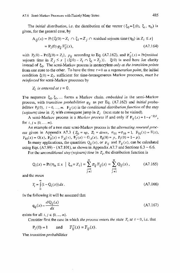
A7.6 Semi-Markov Processes with Finitely Many States 485
The initial distribution, i.e. the distribution of the vector (50- 5(0), Ci, qo) is given, for the general case, by
A u (X) = Pr{ e(0) = Zi n ei = Z n residual sojourn time (qo) in Zi I X 1
with Pi(0) = Pr{k(0) = Zi}, pij according to Eq. (A7.162), and Fij (X) = Priresidual sojourn time in Zj I x 1 (k(0) = Zi n = Zj ) } . k(0) is used here for clarity instead of kO. The semi-Markov process is memoryless only at the transition points from one state to the other. To have the time t = O as a regeneration point, the initial condition c(0) = Zi, sufficient for time-homogeneous Markov processes, must be reinforced for serni-Markov processes by
Zi is entered at t = 0 .
The sequence kO, Cl, ... forms a Markov chain, embedded in the serni-Markov process, with transition probabilities pij as per Eq. (A7.162) and initial proba- bilities Pi(0), i = 0, . . . , m. F, (X) is the conditional distribution function of the stay (sojourn) time in Zi with consequent jump in Zj (next state to be visited).
A semi-Markov process is a Markov process if and only if Fij (X) = 1 -e-PiX,
for i , j E {0, ... , m]. An example of a two state semi-Markov process is the altemating renewal proc-
ess given in Appendix A7.3 (?o = up, Z1 = down, pol =p10 = 1, FO1(x) = F("),
Flo(x) = G(x), Fo(x) = FA(^), FI (X) = GA(x), Po(0) = P , P1(0) = 1 - P ) . In many applications, the quantities QV (X), or pV and Fij (X), can be calculated
using Eqs. (A7.99) - (A7.101), as shown in Appendix A7.7 and Sections 6.3 - 6.6. For the unconditional stay (sojoum) time in Zi, the distribution function is
and the mean
In the following it will be assumed that
exists for all i, j E {0, ..., m]. Consider first the case in which the process enters the state Zi at t = 0, i.e. that
P i ( 0 ) = l and F i ( x ) = F u ( x ) .
The transition probabilities
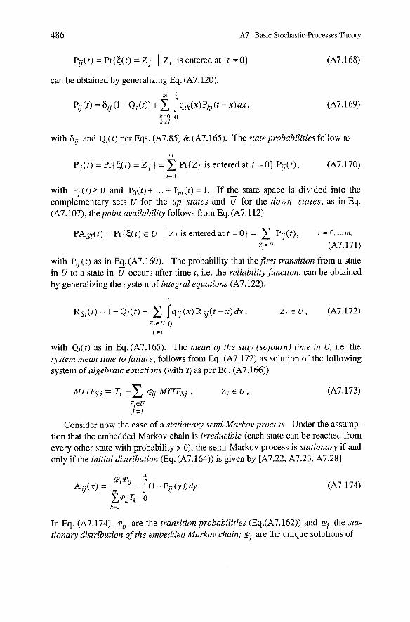
486 A7 Basic Stochastic-Processes Theory
P Q ( ~ ) = Pr{&t) = Z j 1 Zi is entered at t = 0 ) (A7.168)
can be obtained by generalizing Eq. (A7.120),
with 6, and Qi(t) per Eqs. (A7.85) & (A7.165). The stateprobabilities follow as
m
Pj( t ) = Pr{c(t) = Z j } = C. Pr{Zi is entered at t = 0} Pij( t ) , (A7.170)
with Pj ( t ) L 0 and Po(t) + . . . + P,(t) = 1. If the state space is divided into the complementary Sets U for the up states and Ü for the down states, as in Eq. (A7.107), the point availability follows from Eq. (A7.112)
PAsi(t) = Pr{k(t) E U I Zi is entered at t = 0 ) = PQ(t), i = 0, ..., m,
zj= U (A7.171)
with P, ( t ) as in Eq. (A7.169). The probability that thefirst transition from a state in U to a state in Ü occurs after time t , i.e. the reliabilityfunction, can be obtained by generalizing the system of integral equations (A7.122).
with Qi(t ) as in Eq. (A7.165). The mean of the stay (sojourn) time in U, i.e. the system mean time to failure, follows from Eq. (A7.172) as solution of the following system of algebraic equations (with as per Eq. (A7.166))
M V F s i = Ti +X p, M T T Q j , Zi E U , (A7.173) Zj€U j + i
Consider now the case of a stationary semi-Markov process. Under the assump- tion that the embedded Markov chain is irreducible (each state can be reached from every other state with probability > O), the semi-Markov process is stationary if and only if the initial distribution (Eq. (A7.164)) is given by [A7.22, A7.23, A7.281
In Eq. (A7.174), P, are the transition probabilities (Eq.(A7.162)) and pj the sta- tionary distribution of the embedded Markov chain; pj are the unique solutions of
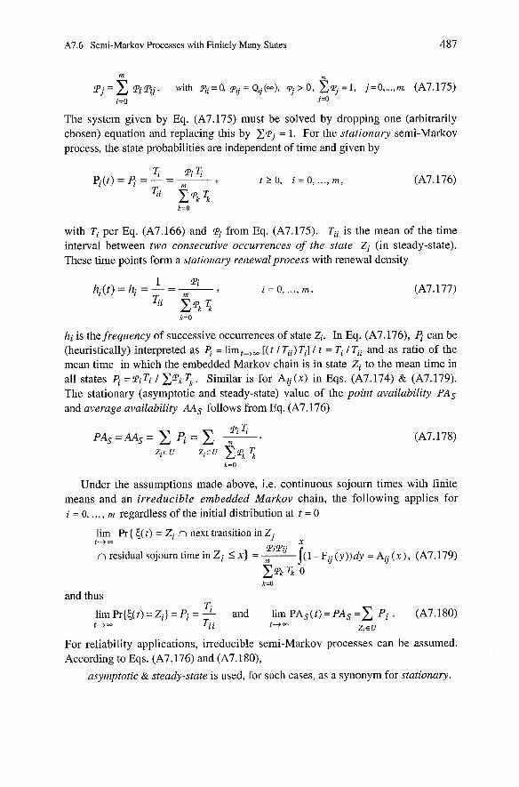
A7.6 Semi-Markov Processes with Finitely Many States 487
The system given by Eq. (A7.175) must be solved by dropping one (arbitrarily chosen) equation and replacing this by E p j = 1. For the stationary semi-Markov process, the state probabilities are independent of time and given by
with Ti per Eq. (A7.166) and Ti from Eq. (A7.175). Tii is the mean of the time interval between two consecutive occurrences of the state Zi (in steady-state). These time points form a stationary renewal process with renewal density
hi is the frequency of successive occurrences of state Zi. In Eq. (A7.176), I j can be (heuristically) interpreted as 4 = lim„, [ ( t I Tii) Ti] 1 t = Ti I Tii and as ratio of the mean time in which the embedded Markov chain is in state Zi to the mean time in all states I;;: = ~ i T i 1 x p k T k . Similar is for A,(x) in Eqs. (A7.174) & (A7.179). The stationary (asymptotic and steady-state) value of the point availability PAs and average availability AAS follows from Eq. (A7.176)
Under the assumptions made above, i.e. continuous sojourn times with finite means and an irreducible embedded Markov chain, the following applies for i = 0, ... , m regardless of the initial distribution at t = 0
lim Pr { &t) = Zi n next transition in Z j t - i m
Pipi X n residual sojourn time in Z i I X} = k l - F , ( y ) ) d y = A , ( x ) , (A7.179)
c . ~ k Tk 0 k=O
and thus Ti l imPr{{ ( t )=Z i )=Pi=- and l i m P A s ( t ) = P A s = x P i . (A7.180)
t+ - Ti i t-im ziel/
For reliability applications, irreducible semi-Markov processes can be assumed. According to Eqs. (A7.176) and (A7.180),
asymptotic & steady-state is used, for such cases, as a synonym for stationary.
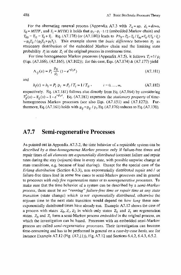
488 A7 Basic Stochastic-Processes Theory
For the alternating renewal process (Appendix A7.3 with Zo = up, Zl =down, T. = MTTF, and Tl = MTTR) it holds that po = pl = 1 / 2 (embedded Markov chain) and T o o = ~ l = T o + ~ . Eq.(A7.178)(or(A7.180))leadsto PAS=Po=ToIT„=ToI(To+T,)
=poTo I (mTO+plTl). This example shows the basic differente between I;. as stationary distribution of the embedded Markov chain and the limiting state probability 8 in state Zi of the original process in continuous time.
For time-homogeneous Markov processes (Appendix A 7 3 , it follows Ti =1/ pi (Eqs. (A7.166), (A7.165), (A7.102)); for this case, Eqs. (A7.174) & (A7.177) yield
and hi(t) = hi= Pi p j =Pi / T i = l /Ti i , i = 0, ..., m , (A7.182)
respectively. Eq. (A7.181) follows also directly from Eq. (A7.164) by considering F; ( X ) = Fg (X) = 1 - e-PiX. Eq. (A7.18 1) expresses the stationary property of time- homogeneous Markov processes (see also Eqs. (A7.15 1) and (A7.127)). Fur- thermore, Eq. (A7.161) holds with pij = pg / pi, Eq. (A7.176) reduces to Eq. (A7.130).
A7.7 Semi-regenerative Processes
As pointed out in Appendix A7.5.2, the time behavior of a repairable system can be described by a time-homogeneous Markov process only if failure-free times and repair times of all elements are exponentially distributed (constant failure and repair rates during the stay (sojourn) time in every state, with possible stepwise change at state transitions, e.g. because of load sharing). Except for the Special case of the Erlang distribution (Section 6.3.3), non exponentially distributed repair and / or failure-free times lead in some few cases to semi-Markov processes and in general to processes with only few regeneration states or to nonregenerative processes. To make sure that the time behavior of a system can be described by a semi-Markov process, there must be no "running" failure-free time or repair time at any state transition (state change) which is not exponentially distributed, otherwise the sojourn time to the next state transition would depend on how long these non- exponentially distributed times have already run. Example A7.12 shows the case of a process with states Zo, Z1, Z2 in which only states Zo and 2, are regeneration states. Zo and Z1 form a semi-Markov process embedded in the original process, on which the investigation can be based. Processes with an embedded semi-Markov process are called semi-regenerative processes. Their investigation can become time-consuming and has to be performed in general on a case-by-case basis, See for instance Example A7.12 (Fig. (A7.1 I)), Fig. A7.12 and Sections 6.4.2,6.4.3,6.5.2.
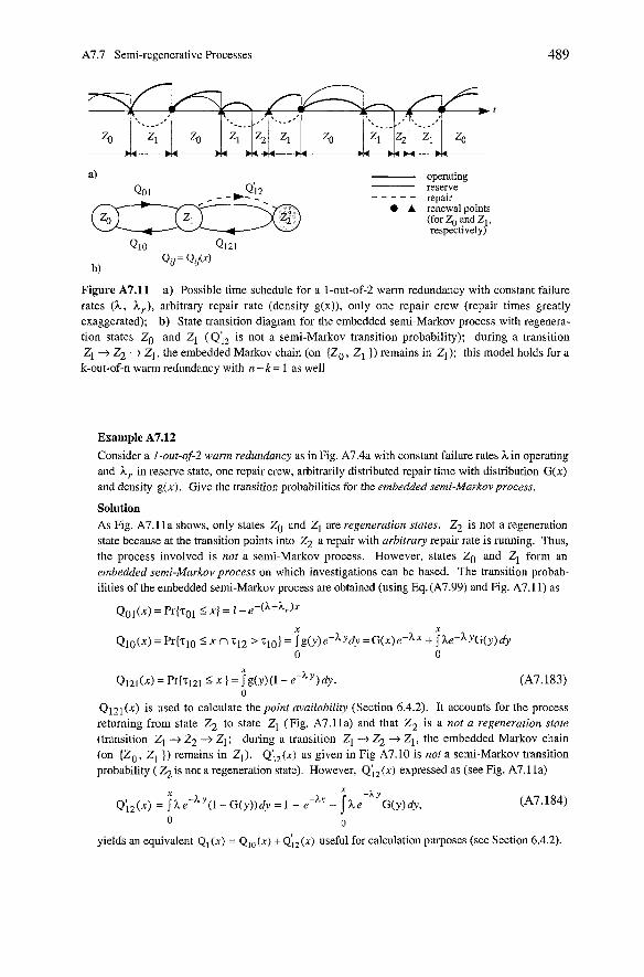
A7.7 Semi-regenerative Processes
- operating reserve - - - - - repair
0 A renewal points (for ZO and Z1, respectively)
Figure A7.11 a) Possible time schedule for a 1-out-of-2 warm redundancy with constant failure rates (L, L,), arbitrary repair rate (density g(x)), only one repair Crew (repair times greatly exaggerated); b) State transition diagram for the embedded semi-Markov process with regenera- tion states ZO and Z1 (Qiz is not a semi-Markov transition probability); during a transition Z1 + % + Z1, the embedded Markov chain (on {Zo , Z, 1) remains in Z1); this model holds for a k-out-of-n warm redundancy with n - k = 1 as well
Example A7.12 Consider a I-out-of-2 warn redundancy as in Fig. A7.4a with constant failure rates h i n operating and h r in reserve state, one repair Crew, arbitrarily distributed repair time with distribution G(x) and density g(x). Give the transition probabilities for the embedded semi-Markovprocess.
Solution As Fig. A7.11a shows, only states ZO and Z1 are regeneration states. % is not a regeneration state because at the transition points into a repair with arbitrary repair rate is running. Thus, the process involved is not a semi-Markov process. However, states ZO and Z1 form an embedded semi-Markov process on which investigations can be based. The transition probab- ilities of the embedded serni-Markov process are obtained (using Eq. (A7.99) and Fig. A7.11) as
Q121(~)= ~ r t q 2 1 5 X I = k y ) ( l - e-'~)dy. (A7.183) 0
Q121(x) is used to calculate the point availability (Section 6.4.2). It accounts for the process returning from state Z2 to state Z1 (Fig. A7.11a) and that Z2 is a not a regeneration state (transition Z1 + Z2 + Z1; during a transition Z1 -t Z2 + Z1, the embedded Markov chain (on {Zo , Z, I) remains in Z1) Qiz(x) as given in Fig A7.10 is not a semi-Markov transition probability ( Z2 is not a regeneration state). However, Q;,(x) expressed as (see Fig. A7.11a)
X -AY Q;,(x) = j h e - " ( l - ~ ( ~ ) ) d y = I - e-" - j h e G(y)dy, (A7.184)
0 0
yields an equivalent Q ~ ( x ) = Qio(x) + Q;~(x) useful for calculation purposes (see Section 6.4.2).
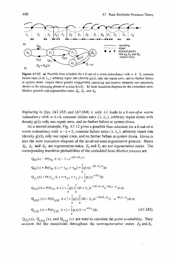
490 A7 Basic Stochastic-Processes Theory
operating - - - - - repair 0 A 7 renewal points
(for ZO, Z1 and ZT, respectively)
Figure A7.12 a) Possible time schedule for a k-out-of-n warm redundancy with n-k =2, constant failure rates (h & L,), arbitrary repair rate (density g(x)), only one repair crew, and no further failure at system down (repair times greatly exaggerated, operating and reserve elements not separately shown in the operating phases at system level); b) State transition diagram for the embedded semi- Markov process with regeneration states Zo , Zl , and Z2,
Replacing in Eqs. (A7.183) and (A7.184) h with kh leads to a k-out-of-n warm redundancy with n-k=l, constant failure rates (h, h,), arbitrary repair times with density g(x), only one repair crew, and no further failure at system down.
As a second example, Fig. A7.12 gives a possible time schedule for a k-out-of-n warm redundancy with n - k = 2 , constant failure rates ( h, L,), arbitrary repair rate (density g(x)), only one repair crew, and no further failure at system down. Given is also the state transition diagram of the involved semi-regenerative process. States ZO, Z1, and Z2. are regeneration states, Z2 and Z3 are not regeneration states. The corresponding transition probabilities of the embedded Semi-Markov process are
Q121(~), Q1232, ( X ) , and Q2,32, (X) are used to calculate the point availability. They account for the transitions throughout the nonregenerative states Z2 andZ3.
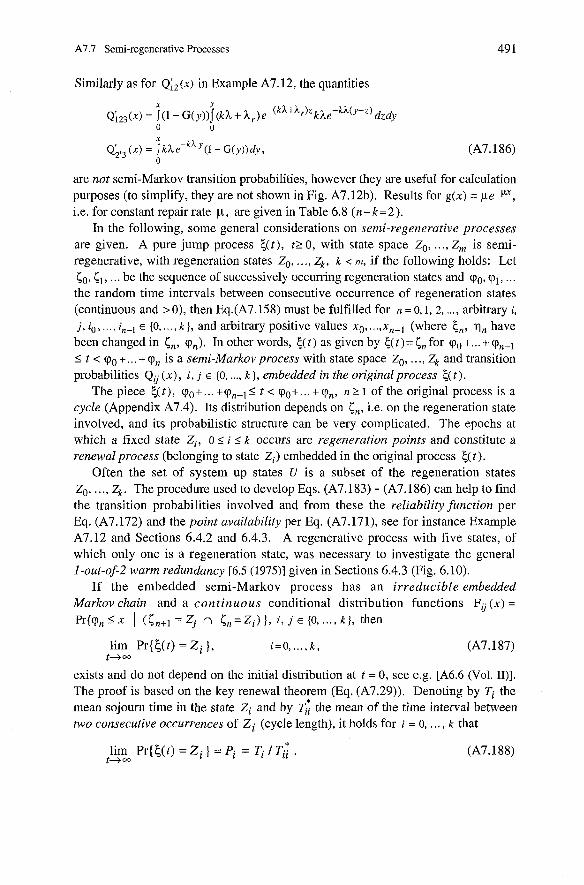
A7.7 Semi-regenerative Processes
Similarly as for Q;,(.w) in Example A7.12, the quantities
are not semi-Markov transition probabilities, however they are useful for calculation purposes (to simplify, they are not shown in Fig. A7.12b). Results for g(x) = pe-P, i.e. for constant repair rate p, are given in Table 6.8 (n-k=2).
In the following, some general considerations on semi-regenerative processes are given. A pure jump process E,(t), tr 0, with state space Zo, . . ., Z, is semi- regenerative, with regeneration states Zo, ..., Zk, k < rn, if the following holds: Let Co, Cl, . . . be the sequence of successively occurring regeneration states and ( P ~ , < P ~ , . . . the random time intervals between consecutive occurrence of regeneration states (continuous and > 0), then Eq.(A7.158) must be fulfilled for n = 0,i, 2, ..., arbitrary i, j, i,, ..., in-l E {O, ..., k ] , and arbitrary positive values XO, ..., x,,-~ (where 5„ q, have been changed in C,„ V,). In other words, E,(t ) as given by E,(t)= 5, for cpo +. .. + <pn-l
2 t < + .. . + 9, is a semi-Markov process with state space Zo, . . ., Zk and transition probabilities Q, ( X ) , i, j E {O, ..., k 1, embedded in the original process E,(t).
The piece E,( t ), (PO+. .. +<P,-~ 5 t < (PO+. . . + (P,, n t 1 of the original process is a cycle (Appendix A7.4). Its distribution depends on C„ i.e. on the regeneration state involved, and its probabilistic structure can be very complicated. The epochs at which a fixed state Zi, 0 s i s k occurs are regeneration points and constitnte a renewal process (belonging to state Zi) embedded in the original process E,(t).
Often the Set of system up states U is a subset of the regeneration states Zo, . . . , Zk. The procedure used to develop Eqs. (A7.183) - (A7.186) can help to find the transition probabilities involved and from these the reliability function per Eq. (A7.172) and the point availability per Eq. (A7.171), see for instance Example A7.12 and Sections 6.4.2 and 6.4.3. A regenerative process with five states, of which only one is a regeneration state, was necessary to investigate the general 1-out-of-2 warm redundancy [6.5 (1975)l given in Sections 6.4.3 (Fig. 6.10).
If the embedded semi-Markov process has an irreducible embedded Markov chain and a continuous conditional distribution functions Fij ( X ) = Pr(<p, 5 X ( (<n+l = Zj n 5, = Zi) 1, i, j E (0, ..., k 1, then
lim Pr{$(t) =Si}, i=O, ..., k , t+ -
exists and do not depend on the initial distribution at t = 0, see e.g. [A6.6 (Vol. II)]. The proof is based on the key renewal theorem (Eq. (A7.29)). Denoting by Ti the mean sojourn time in the state Zi and by T; the mean of the time interval between two consecutive occurrences of Zi (cycle length), it holds for i = 0, .. . , k that
lim Pr{c(t) = Si J = Pi = Ti / T; t+
492 A7 Basic Stochastic-Processes Theory
For the 1 -out-of-2 warm redundancy of Example A7.12 it holds that PO = P I = 1 1 2
(embeddedMarkovchain), T o = l l ( h + h r ) , T 1 = ( l - & h ) ) l h , T & = l l ( h + h , ) + M ~ T R
+ [ ( I - g ( h ) ) l g ( h ) ] M l ~ R , T ~ = ~ ( ~ ) [ ~ / ( ~ + ~ , ) + M T T R ] + ( ~ - ~ ( ~ ) ) M T T R , P, =To/T&, and P, = Zi I T,;. The final result for PAs = Po +P, is given by Eq. (6.109). For constant repair rate p , g(h) = p l ( h + p ) and T. = 1 l ( h + h , ) , Tl = l / ( h + P), Tio =
( p 2 + ( h + h r ) ( h + p ) ) l p 2 ( h + h r ) , T; = ( p 2 + ( h + h r ) ( h + P ) ) l p ( h + h r ) ( h + P ) , yielding PAs =Po + P, = T. /T& + Tl /T,; according to Eq.(6.88), or Eq.(A7.152) for h„=h; this case can also be investigated considering 3 regeneration states as per Fig. 6.8a.
A7.8 Nonregenerative Stochastic Processes
The assumption of arbitrarily (i.e. not exponentially) distributed failure-free and repair (restoration) times for the elements of a system, already leads to nonregener- ative stochastic processes for simple series or parallel structures. After some general considerations, nonregenerative processes used in reliability analysis are introduced.
A7.8.1 General Considerations
Solutions for nonregenerative stochastic processes are often problem-oriented. However, as a possible general method, transformation of the given stochastic process into a Markov or a semi-Markov process by a suitable state space extension can be used in some cases by one of the following ways:
1. Approximation of distribution functions: Approximating the involved distri- bution functions (for repair andlor failure-free times) by an Erlang distribution (Eq. (A6.102)) allows a transformation of the original process into a time- homogeneous Markov process through introduction of additional states.
2. Introduction of supplementary variables: Introducing for every element of a system as supplementary variables the failure-free time since the last repair and the repair time since the last failure, the original process can be transformed into a Markov process with state space consisting of discrete and continuous Parameters. Investigations usually lead to partial differential equations which have to be solved with the corresponding boundary conditions.
The first method is best used when repair andlor failure rates are monotonically increasing from Zero to a final value, its application is easy to understand (Fig. 6.6). The second method [A7.4 (1955)l is very general, but often time-consuming.
A7.8 Nonregenerative Stochastic Processes 493
A further method is based on the general concept of point process. Considering the sequence of jump times T; and states 5, entered at these points, an equivalent description of the process ((t) is obtained by a marked point process (T:, C,), n=O, 1, ... . Analysis of the system's steady-state behavior follows using Korolyuk's theorem ( Pr{ jump into Zi during ( t, t At] } = ht 6t + o(6t), with =E [Number of jumps in Zi during the unit time interval]), See e.g. [A7.11, A7.121. As an example, consider a repairable coherent system with n totally independent elements (p. 61). Let C 1 ( t ) , . . . , CJt) and <(t) be the binary processes with states 0 (down) & 1 (up) describing ele-
ments and system, respectively. If the steady-state point availability of each element
M T 6 lim PAi(t) = lim Pr{ci(t) = 1) = PAi = i= l , ..., n, (A7.189) t+- t+m M 7 T q + M T R i '
exists, then the steady-state point availability of the system is given by Eq. (2.48) and can be expressed as PAs = MTTFs / (MTTFs + MTTRs), see e.g. [6.4, A7.101.
Investigation of the time behavior of Systems with arbitrary failure andor repair rates can become time-consurning. In these cases, approximate expressions can help to get results (see Section 6.7 for some examples).
A7.8.2 Nonhomogeneous Poisson Processes (NHPP)
A nonhomogeneous Poisson process (NHPP) is a point process with independent Poisson distributed increments, i.e. a sequence of points (events) on the time axis, which Count function V ( t ) has independent increments (in nonoverlapping intervals) and satisfy
V ( t) gives the number of events in (0, t]. In the following, V ( t ) is assumed right continuous with unit jumps. M(t) is the mean of V ( t ) , called mean valuefunction,
M(t) = E [ ~ ( t ) ] , t>O, M(O)=O, (A7.191)
and it holds that (Example A6.20)
Var [ ~ ( t ) ] = E [ ~ ( t ) ] = M(t), t>O, M(O)=O. (A7.192)
M(t) is a nondecreasing, continuous function with M(0) = 0, often assumed increasing, unbounded, and absolutely continuous. If
m(t) = dM(t) / dt 2 0 , t>O, (A7.193)
exists, m(t) is the intensity of the NHPP. Eqs. (A7.193) and (A7.19 1) yield
Pr{v(t+6t) - ~ ( t ) = l } = m(t) 6 t + o(6t), t>O,6t.L0, (A7.194)
and no distinction is made between arrival rate and intensiv. Equation (A7.194)
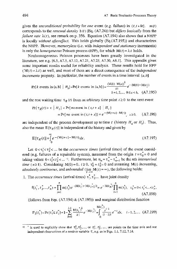
494 A7 Basic Stochastic-Processes Theory
gives the unconditional probability for one event (e.g. failure) in ( t , t + St] . m(t) corresponds to the renewal den& h ( t ) (Eq. (A7.24)) but dijjfers basically from the failure rate A( t ) , see remark on p. 356. Equation (A7.194) also shows that a NHPP is locally without aftereffect. This holds globally (Eq.(A7.195)) and characterizes the NHPP. However, memoryless (i.e. with independent und stationary increments) is only the homogeneous Poisson process (HPP), for which M ( t ) = t holds.
Nonhomogeneous Poisson processes have been greatly investigated in the literature, see e.g. [6.3, A7.3, A7.12, A7.21, A7.25, A7.30, A8.11. This appendix gives some important results useful for reliability analysis. These results hold for H P P ( M ( t ) = A t ) as well, and most of them are a direct consequence of the independent increments property. In particular, the number of events in a time interval ( U , b]
m w - ~ i , ) i ' ,- (M(S)-M(,,)) Pr{k events in (a, b] I Ha] =Pr{k events in (a, b] ] = k !
k=1,2 ,..., O l a < b , (A7.195)
and the rest waiting time Z R ( t ) from an arbitrary time point t 2 0 to the next event
P r { ~ ~ ( t ) > x I H,]=Pr{noevent in( t , t+x] I H , )
=Pr{no event i n ( t , t + x ] ] = e -("(t+x)-M(t)) 0, (A7.196)
are independent of the process development up to time t (history H, or H,). Thus, also the mean E [ ~ ~ ( t ) ] is independent of the history and given by
Let 0 < T{< 22 < . . . be the occurrence times (arrival times) of the event consid- ered (e.g. failures of a repairable system), measured from the origin t = T ; = 0 and
* * taking values O< t: t i < ... +). Furthermore, let q, = T , - T , - ~ be the nth interarrival time ( n 2 1). Considering M(0) = 0 , t 2 0 , T ; = t ; = 0 and assurning M(t) increasing, absolutely continuous, and unbounded (lim M ( t ) = M), the following holds:
t+m
1. The occurrence times (arrival times) T;, 22 ,... have joint density n * * * * * * *
f(t, , t „ ..., t i ) =nm(ty)e-(M(ti)-M(ti-l))= e - M ( t n ) n m ( t i ) , t o =o< t l < ... <t;, i=l i=l (A7.198)
(follows from Eqs. (A7.194) & (A7.195)) and marginal distribution function
+) * is used to explicitly show that 2;,22, ..., or t f , t i , ..., are points on the time axis and not independent observations of a random variable 2, e.g. as in Figs. 1.1,7.12,7.14.
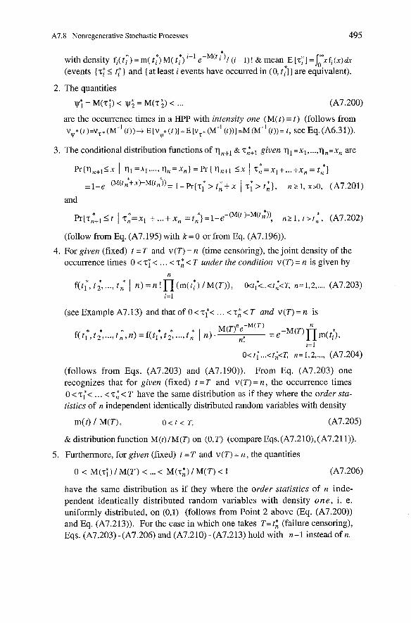
A7.8 Nonregenerative Stochastic Processes 495
* with density fi(tT) = m( t l ) ~ ( t:) " e-M(ti )/ (i - I ) ! & mean E [T:] = / : x f i ( x ) d r
(events { T ; 5 t,' } and {at least i events have occurred in (0 , t ; ] ) are equivalent).
2. The quantities
V*, = M(T;) < = M(T 2) < ...
are the occurrence times in a HPP with intensity one ( M ( t ) = t ) (follows from V,. ( t ) = v T * (M-' ( t ) ) + E [ v . ( t ) l = E [V=* (M-' ( t ) ) ] =M (M-' ( t ) ) = t , see Eq. (A6.31)).
V
3. The conditional distribution functions of q„l & T:+~ given q l = x l , ...,V„= X, are
(follow from Eq. (A7.195) with k = 0 or from Eq. (A7.196)).
4. For given (fixed) t = T and v ( T ) = n (time censoring), the joint density of the occurrence times 0 < T ; < . . . < T ; < T under the condition v ( T ) = n is given by
(see Example A7.13) and that of 0 < T;< . . . T ; < T und v ( T ) = n is
(follows from Eqs. (A7.203) and (A7.190)). From Eq. (A7.203) one recognizes that for given (fixed) t =T and v ( T ) = n , the occurrence times 0 <T;< . . . < T ; < T have the same distribution as if they where the order sta- tistics of n independent identically distributed random variables with density
& distribution function M ( t ) l M ( T ) on (0, T ) (compare Eqs.(A7.210), (A7.211)).
5. Furthermore, for given (fixed) t =T and V (T) = n , the quantities
have the same distribution as if they where the order statistics of n inde- pendent identically distributed random variables with density o n e , i. e. uniformly distributed, on (0 , l ) (follows from Point 2 above (Eq. (A7.200)) and Eq. (A7.213)). For the case in which one takes T= t i (failure censoring), Eqs. (A7.203) - (A7.206) and (A7.210) - (A7.213) hold with n-1 instead of n.
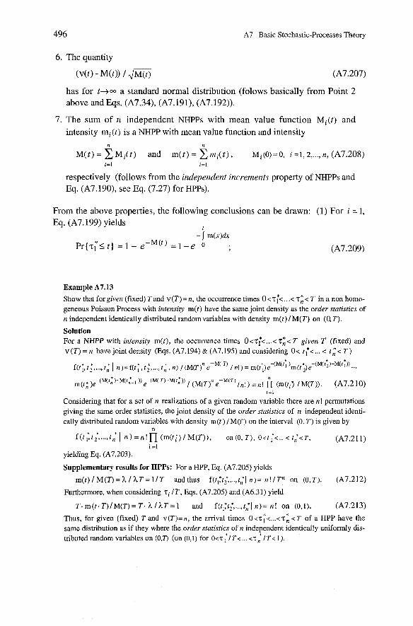
A7 Basic Stochastic-Processes Theory
has for t - + m a standard normal distribution (folows basically from Point 2 above and Eqs. (A7.34), (A7. lgl), (A7.192)).
7. The sum of n independent NHPPs with mean value function M,(t) and intensity mi ( t ) is a NHPP with mean value function and intensity
i=l i=l
respectively (follows from the independent increments property of NHPPs and Eq. (A7.190), see Eq. (7.27) for HPPs).
From the above properties, the following conclusions can be drawn: (1) For i = 1,
Eq. (A7.199) yields t
- I m(x)dx ~ r { ~ l l t } = 1 - e-"(t) = 1 -e 0 ; (A7.209)
Example A7.13 Show that for given (fixed) T and V (T) = n, the occurrence times 0 <T:<. . .< T; < T in a non homo- geneous Poisson Process with intensity m(t) have the Same joint density as the order statistics of n independent identically distnbuted randomvariables with density m(t)l M ( T ) on (0, T).
Solution For a NHPP with intensity m(t), the occurrence times O<T~< ... < T;< T given T (fixed) and V (T) = n have joint density (Eqs. (A7.194) & (A7.195) and considering 0< t;< ... < t :< T )
f(t;,t;, ..., t l 1 n)=f( t ; , t l ,..., t i , n) / (M(T)~ e-M(71 /n!) = m(t;)e-(M(';)m(t~)e-(M('~)-M(';))...
m(tn „-(M(ti )-M(Z;_, )) e-(M( 'O-Wt: j) / (M(T)" e-"(T',n! ) =n! fi (m(til /M(T)). (A7.210) i=l
Considering that for a Set of n realizations of a given random variable there are n! permutations giving the same order statistics, the joint density of the order statistics of n independent identi- cally distributed random variables with density m(t) 1 M(T) on the interval (0, T) is given by
f ( t ; t c ..., t i 1 n ) = n ! n (m(t i ) lM(T)) , on(0, T), ~ < t ; < ... < t , '<~, (A7.211) i =l
yielding Eq. (A7.203).
Supplementary results for HPPs: For a HPP, Eq. (A7.205) yields
m(t) / M(T) = h / h T = 1 / T and thns f(t,:tG,..,t,'l n)= n!lTn on (0,T). (A7.212)
Furthermore, when considering 'ci /T, Eqs. (A7.205) and (A6.31) yield
T.m(t . T) /M(T)= T. h / h T = l and f(tl:t$ ..., t,*l n ) = n! on (0,s). (A7.213)
Thus, for given (fixed) T and v(T)=n, the arrival times 0<'c;< ... <T: < T of a HPP have the same distnbution as if they where the order statistics of n independent identically uniformly dis- tributed random variables on (0,T) (on (0,s) for O<T ; /T< ... <T; /T< 1).
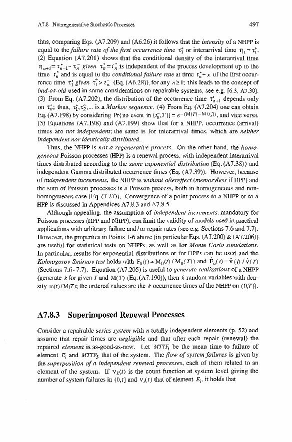
A7.8 Nonregenerative Stochastic Processes 497
thus, comparing Eqs. (A7.209) and (A6.26) it follows that the intensit~ of a NHPP is equal to the failure rate of the first occurrence time T: or interarrival time V, = 7;.
(2) Equation (A7.201) shows that the conditional density of the interarrival time v ~ + ~ = T;+~- T; given T; = tn is independent of the process development up to the time t,* and is equal to the conditional failure rate at time t i+ x of the first occur- rence time T; given T; > t i (Eq. (A6.28)), for any n? 1; this leads to the concept of bad-as-old used in some considerations on repairable Systems, see e.g. [6.3, A7.301. (3) From Eq. (A7.202), the distribution of the occurrence time zL1 depends only on T;; thus, T;, 22, ... is a Markov sequence. (4) From Eq. (A7.204) one can obtain Eq. (A7.198) by considering Pr{ no event in ( t i , T ] ] = e- (M(T)-M@,?), and vice versa. (5) Equations (A7.198) and (A7.199) show that for a NHPP, occurrence (arrival) times are not independent; the same is for interarrival times, which are neither independent nor identically distributed.
Thus, the NHPP is not a regenerative process. On the other hand, the homo- geneous Poisson processes (HPP) is a renewal process, with independent interarrival times distributed according to the same exponential distribution (Eq. (A7.38)) and independent Gamma distributed occurrence times (Eq. (A7.39)). However, because of independent increments, the NHPP is without aftereffect (memoryless if HPP) and the sum of Poisson processes is a Poisson process, both in homogeneous and non- homogeneous case (Eq. (7.27)). Convergence of a point process to a NHPP or to a HPP is discussed in Appendices A7.8.3 and A7.8.5.
Although appealing, the assumption of independent incrernents, mandatory for Poisson processes (HPP and NHPP), can limit the validity of models uscd in practical applications with arbitrary failure andlor repair rates (see e.g. Sections 7.6 and 7.7). However, the properties in Points 1-6 above (in particular Eqs. (A7.200) & (A7.206)) are useful for statistical tests on NHPPs, as well as for Monte Carlo simulations. In particular, results for exponential distributions or for HPPs can be used and the Kolmogorov-Smirnov test holds with Fo(t) = Mo(t) l Mo(T)) and I?,( t ) = G ( t) 1 ( T )
(Sections 7.6- 7.7). Equation (A7.205) is useful to generate realizations of a NHPP (generate k for given T and M(T) (Eq. (A7.190)), then k random variables with den- sity m(t) / M ( T ) ; the ordered values are the k occurrence times of the NHPP On (0,T)) .
A7.8.3 Superimposed Renewal Processes
Consider a repairable series system with n totally independent elements (p. 52) and assume that repair times are negligible and that after each repair (renewal) the repaired element is as-good-as-new. Let be the mean time to failure of element Ei and M T T 6 that of the system. Theflow of system failures is given by the superposition of n independent renewal processes, each of them related to an element of the system. If vs ( t ) is the Count function at system level giving the number of system failures in (O,t] and v i ( t ) that of element Ei, it holds that
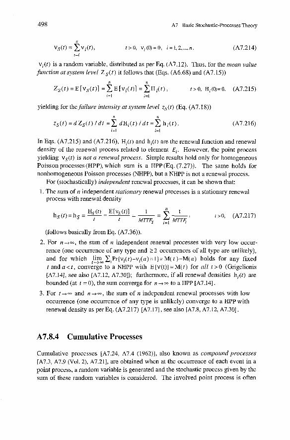
498 A7 Basic Stochastic-Processes Theory
n
VS(~) = E v i ( t ) , t>O, vi(0)=O, i = l , 2 ,..., n . (A7.214) i=l
vi(t) is a random variable, distributed as per Eq. (A7.12). Thus, for the rnean value finction a t System level Zs( t ) it follows that (Eqs. (A6.68) and (A7.15))
yielding for the failure intensiq a t systern level zS(t) (Eq. (A7.18))
In Eqs. (A7.215) and (A7.216), Hi(t) and hi(t) are the renewal function and renewal density of the renewal process related to element Ei. However, the point process yielding vS(t) is not a renewal process. Simple results hold only for homogeneous Poisson processes (HPP), which surn is a HPP (Eq. (7.27)). The Same holds for nonhomogeneous Poisson processes (NHPP), but a NHPP is not a renewal process.
For (stochastically) independent renewal processes, it can be shown that:
1. The surn of n independent stationary renewal processes is a stationary renewal process with renewal density
(follows basically from Eq. (A7.36)).
2. For n - t - , the surn of n independent renewal processes with very low occur- rence (one occurrence of any type and 2 2 occurrences of all type are unlikely), and for which ?imm Zipr{vi(t)-vi(a) =I}= M( t )-M(a) holds for any fixed t and a < t , converge to a NHPP with E [ ~ ( t ) ] = M(t) for a l l t > 0 (Grigelionis rA7.141, see also [A7.12, A7.301); furthermore, if all renewal densities hi(t) are bounded (at t = O), the sum converge for n -1- to a HPP [A7.14].
3. For t -1- and n+-, the surn of n independent renewal processes with low occurrence (one occurrence of any type is unlikely) converge to a HPP with renewal density as per Eq. (A7.217) [A7. 171, See also [A7.8, A7.12, A7.301.
A7.8.4 Cumulative Processes
Cumulative processes [A7.24, A7.4 (1962)j, also known as compound processes [A7.3, A7.9 (Vol. 2), A7.211, are obtained when at the occurrence of each event in a point process, a random variable is generated and the stochastic process given by the surn of these random variables is considered. The involved point process is often
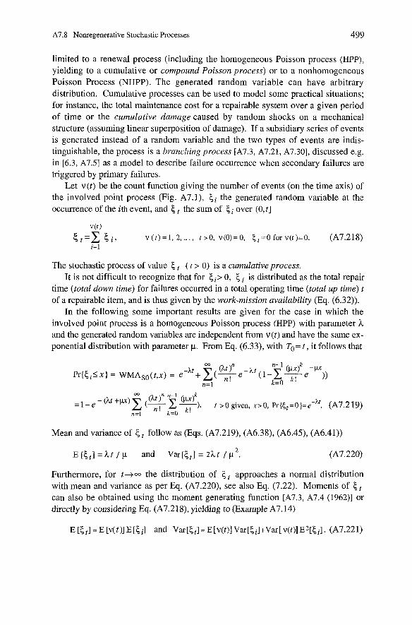
A7.8 Nonregenerative Stochastic Processes 499
limited to a renewal process (including the homogeneous Poisson process (HPP), yielding to a cumulative or compound Poisson process) or to a nonhomogeneous Poisson Process (NHPP). The generated random variable can have arbitrary distribution. Cumulative processes can be used to model some practical situations; for instance, the total maintenance cost for a repairable system over a given period of time or the cumulative damage caused by random shocks on a mechanical structure (assuming linear superposition of damage). If a subsidiary senes of events is generated instead of a random variable and the two types of events are indis- tinguishable, the process is a branching process [A7.3, A7.21, A7.301, discussed e.g. in [6.3, A7.51 as a model to describe failure occurrence when secondary failures are triggered by primary failures.
Let ~ ( t ) be the count function giving the number of events (on the time axis) of the involved point process (Fig. A7.1), C i the generated random variable at the occurrence of the ith event, and 5, the sum of 5 over (0,tl
The stochastic process of value 6 , ( t > 0) is a cumulative process. It is not difficult to recognize that for t i > 0, 5 is distributed as the total repair
time (total down time) for failures occurred in a total operating time (total up time) t of a repairable item, and is thus given by the work-mission availability (Eq. (6.32)).
In the following some important results are given for the case in which the involved point process is a homogeneous Poisson process (HPP) with parameter h and the generated random variables are independent from V (t) and have the same ex- ponential distribution with parameter p. From Eq. (6.33), with To= t , it follows that
(At )n n-l =I-e- (~ t f~)x ) . t > o given. n o . pr{&=o)=e-? (A7.219) n =l
Mean and variance of 5, follow as (Eqs. (A7.219), (A6.38), (A6.45), (A6.41))
Furthermore, for t+m the distribution of 5, approaches a normal distribution with mean and variance as per Eq. (A7.220), see also Eq. (7.22). Moments of 5 , can also be obtained using the moment generating function [A7.3, A7.4 (1962)l or directly by considering Eq. (A7.218), yielding to (Example A7.14)
E [St] = E [v(t)] E[ki] and ~ a r [ ~ ~ ] = E [ v ( t ) l ~ a r [ ~ ~ l + ~ a r [ v ( t ) ] ~ ~ [ ~ ~ l . (A7.221)
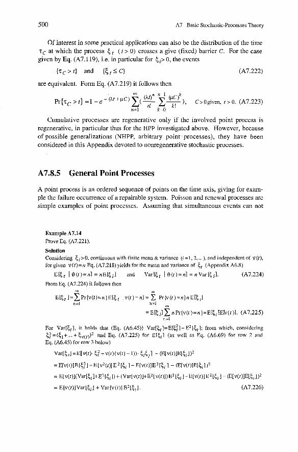
500 A7 Basic Stochastic-Processes Theory
Of interest in some practical applications can also be the distribution of the time at which the process 5 , ( t > 0) crosses a give (fixed) barrier C. For the case
given by Eq. (A7.119), i.e. in particular for ki> 0, the events
{ z c > t ] and { t t 5 C } (A7.222)
are equivalent. Form Eq. (A7.219) it follows then
Cumulative processes are regenerative only if the involved point process is regenerative, in particular thus for the HPP investigated above. However, because of possible generalizations (NHPP, arbitrary point processes), they have been considered in this Appendix devoted to nonregenerative stochastic processes.
A7.8.5 General Point Processes
A point process is an ordered sequence of points on the time axis, giving for exam- ple the failure occurrence of a repairable System. Poisson and renewal processes are simple examples of point processes. Assuming that simultaneous events can not
Example A7.14 Prove Eq. (A7.221).
Solution Considering 5 >O, continuous with finite mean & variance (i = 1,2, ... ), and independent of V (t), for given V(t)=n Eq. (A7.218) yields for the mean and variance of tt (Appendix A6.8)
E[c t I 6 ( t ) = n l = nElci l and Varlct I B( t )=nl = nVar[cil . (A7.224)
From Eq. (A7.224) it follows then
For Var& 1, it holds that (Eq. (A6.45)) ~ a r [ < ~ ] = ~ [ c : ] - E2 [ C t ] ; from which, considering =(Ci+ ... + cv(t))2 and Eq. (A7.225) for (as well as Eq. (A6.69) for row 2 and
Eq. (A6.45) for row 3 below)
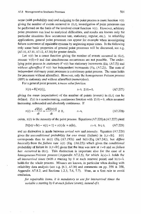
A7.8 Nonregenerative Stochastic Processes 501
occur (with probability one) and assigning to the point process a count function v ( t ) giving the number of events occurred in (O,t], investigation of point processes can be performed on the basis of the involved count function ~ ( t ) . However, arbitrary point processes can lead to analytical difficulties, and results are known only for particular situations (low occurrence rate, stationary, regular, etc.). In reliability applications, general point processes can appear for example when investigating failure occurrence of repairable Systems by neglecting repair times. In the following only some basic properties of general point processes will be discussed, see e.g. [A7.10, A7.11, A7.12, A7.301 for greater details.
Let ~ ( t ) be a count function giving the number of events occurred in (O,t], assume v(O)= 0 and that simultaneous occurrences are not possible. The under- lying point process is stationary if v ( t ) has stationary increments (Eq. (A7.5)) and without aftereffect if v ( t ) has independent increments (Eq. (A7.2)). The sum of independent stationary point processes is a stationary point process. The same holds for processes without aftereffect. However, only the homogeneous Poisson process ( H P P ) is stationary und without aftereffect (memoryless).
For a general point process, a mean value function
giving the mean (expectation) of the number of points (events) in (O,t] can be defined. Z( t ) is a nondecreasing, continuous function with Z(0) = 0, often assumed increasing, unbounded and absolutely continuous. If
exists, z(t) is the intensity of the point process. Equations (A7.228)&(A7.227) yield
and no distinction is made between arrival rate and intensity. Equation (A7.229) gives the unconditional probability for one event (failure) in (t, t +6t]. ~ ( t ) corresponds thus to m( t ) (Eq. (A7.193)) and h(t) (Eq. (A7.24)), but differs basically from the failure rate h(t) (Eq. (A6.25)) which gives the conditional probability of failure in (t , t +6t] given that the item was new at t = 0 and no failure has occurred in (O,t]. This distinction is important also for the case of a homogeneous Poisson process (Appendix A7.2.5), for which h(x)= A holds for all interarrival times (with x starting by 0 at each renewal point) and h(t)=A holds for the whole process. Misuses are known, in particular when dealing with reliability data analysis (see e.g. [6.3, A7.301 and comments on pp. 356 & 358, Appendix A7.8.2, and Sections 1.2.3, 7.6, 7.7). Thus, as a first rule to avoid confusion,
for repairable items, it is mandatory to use for interarrival times the variable x starting by 0 at each failure (event), instead oft.
502 A7 Basic Stochastic-Processes Theory
Some limits theorems on point processes are known, in particular on the convergence to a HPP, See e.g. [A7.10, A7.11, A7.121.
In reliability applications, z(t) is called failure intensi9 [A1.4], ROCOF (rate of occurrence of failures) in [6.3] . z(t) applies in particular to repairable Systems when repair (restoration) times are neglected. In this case, vs ( t ) is the Count function giving the number of system failures occurred in (O,t], with ~ ( 0 ) = 0, and
is the system failure intensity.
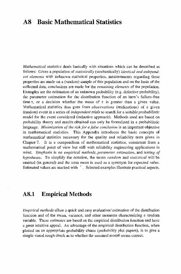
Ag Basic Mathematical Statistics
Mathematical statistics deals basically with situations which can be described as follows: Given a population of statistically (stochastically) identical und independ- ent elements with unknown statistical properties, measurements regarding these properties are made on a (random) sample of this population and on the basis of the collected data, conclusions are made for the remaining elements of the population. Examples are the estimation of an unknown probability (e.g. defective probability), the parameter estimation for the distribution function of an item's failure-free time T, or a decision whether the mean of T is greater than a given value. Mathematical statistics thus goes from observations (realizations) of a given (random) event in a series of independent trials to search for a suitableprobabilistic model for the event considered (inductive approach). Methods used are based on probability theory and results obtained can only be formulated in a probabilistic language. Minimization of the risk for a false conclusion is an important objective in mathematical statistics. This Appendix introduces the basic concepts of mathematical statistics necessary for the quality and reliability tests given in Chapter 7. It is a compendium of mathematical statistics, consistent from a mathematical point of view but still with reliability engineering applications in mind. Emphasis is on empirical methods, parameter estimation, and testing of hypotheses. To simplify the notation, the terms random and statistical will be omitted (in general) and the term mean is used as a synonym for expected value. Estimated values are marked with " . Selected examples illustrate practical aspects.
A8.1 Empirical Methods
Empirical methods allow a quick and easy evaluationl estimation of the distribution function and of the mean, variance, and other moments characterizing a random variable. These estimates are based on the empirical distribution function and have a great intuitive appeal. An advantage of the empirical distribution function, when plotted on an appropriate probability charts (probability plot papers), is to give a simple visual rough check as to whether the assumed model seems correct.
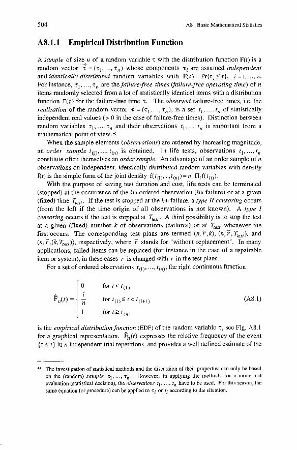
504 A8 Basic Mathematical Statistics
A8.1.1 Empirical Distribution Function
A sample of size n of a random variable T with the distribution function F(t) is a -+
random vector T = ( z l , ..., T, ) whose components zi are assumed independent and identically distributed random variables with F(t) = Pr{zi < t } , i = 1 , ..., n.
For instance, T I , ..., T , are the failure-free times (failure-free operating time) of n items randomly selected from a lot of statistically identical items with a distribution function F(t) for the failure-free time T. The obsewed failure-free times, i.e. the
+ realization of the random vector z = ( z l , ..., T,), is a set t l , ..., t , of statistically independent real values (> 0 in the case of failure-free times). Distinction between random variables z l , . . . , T , and their observations t l , . . ., t , is important from a mathematical point of view. +)
When the sample elements (obsewations) are ordered by increasing magnitude, an order sample t ( l ) , ..., t(,) is obtained. In life tests, observations t l , ..., t , constitute often themselves an order sample. An advantage of an order sample of n observations on independent, identically distributed random variables with density f(t) is the simple form of the joint density f(t(l),...,t(,)) = n ! IIi f( t( i)) .
With the purpose of saving test duration and cost, life tests can be terminated (stopped) at the occurrence of the kth ordered observation (kth failure) or at a given (fixed) time T„, . If the test is stopped at the kth failure, a type II censoring occurs (from the left if the time origin of all observations is not known). A type I censoring occurs if the test is stopped at T„, . A third possibility is to stop the test at a given (fixed) number k of observations (failures) or at Te„, whenever the first occurs. The corresponding test plans are termed (n, F,k), (n,F, T„,), and (n, F,(k,T„,)), respectively, where F stands for "without replacement". In many applications, failed items can be replaced (for instance in the case of a repairable item or system), in these cases F is changed with r in the test plans.
For a set of ordered observations t ( l ) , ..., t(,), the right continuous function
for t < t ( l )
for t ( , ) < t < t ( i + i ) (A8.1)
for t 2 t ( , )
is the empirical distributionfunction (EDF) of the random variable T, See Fig. A8.1 for a graphical representation. fi,(t) expresses the relative frequency of the event ( T 5 t } in n independent trial repetitions, and provides a well defined estimate of the
+) The investigation of statistical methods and the discussion of their properties can only be based on the (random) sample T I , ..., T,. However, in applying the methods for a numencal evaluation (statistical decision), the observations tl, ..., tn have to be used. For this reason, the sarne equation (or procedure) can be applied to or ti according to the situation.

A8.1 Empirical Methods
L."
Figure A8.1 Example of an empirical distribution function (t,, ..., t, t ( l ), ..., t ( , is assumed here)
distribution function F(t) = Pr{z 2 t}. The symbol - is hereafter used to denote an estimate of an unknown quantity. As stated in the footnote on p. 504, when investigating the properties of the empirical distribution function F,(t) it is necessary in Eq. (A8.1) to replace the observations t(l),..., t(,) by the sample elements T(I ) , . . ., T(,) .
For given F(t) and any fixed value of t, the number of observations I t, i.e. n I?,(t), is binomially-distributed (Eq. (A6.120)) with Parameter p = F(t), mean
E [n fin (t)] = n F(t) , (A8.2)
and variance
~ a r [n fi, (t)] = n F(t) (1 - F(t)). (A8. 3)
Moreover, application of the strong law of large numbers (Eq. (A6.146)) shows that for any given (fixed) value o f t , I?,(t) converges to F(t) with probability one for n -+ m. This convergence is uniform in t and holds for the whole distribution function F(t). Proof of this important result is given in the Glivenko-Cantelli theorem [A8.4, A8.14, A8.161, which states that the largest absolute deviation between I?,(t) and F(t) over all t, i.e.
converges with probability one toward 0
Pr{ lim D, = 0 } = 1. H-
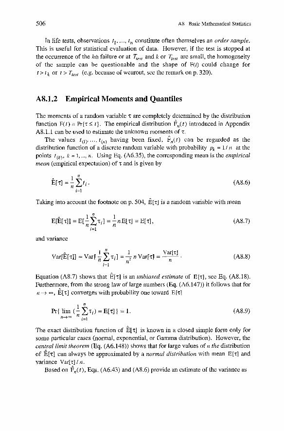
506 A8 Basic Mathematical Statistics
In life tests, observations t l , .. ., t , constitute often themselves an order sample. This is useful for statistical evaluation of data. However, if the test is stopped at the occurrence of the kth failure or at S„, and k or T„„ are small, the homogeneity of the sample can be questionable and the shape of F(t) could change for t > t k or t > T„, (e.g. because of wearout, See the remark on p. 320).
A8.1.2 Empirical Moments and Quantiles
The moments of a random variable T are completely determined by the distribution function F(t) = Pr{z I t ) . The empirical distribution e,(t) introduced in Appendix A8.1.1 can be used to estimate the unknown moments of T .
The values t( l) , ..., t(,) having been fixed, 6 J t ) can be regarded as the distribution function of a discrete random variable with probability pk = 11 n at the points t ( k ) , k = 1, ..., n. Using Eq. (A6.35), the corresponding mean is the empirical mean (empirical expectation) of T and is given by
Taking into account the footnote on p. 504, E[%] is a random variable with mean
and variance
Equation (A8.7) shows that E[T] is an unbiased estimate of E [ z ] , see Eq. (A8.18). Furthermore, from the strong law of large numbers (Eq. (A6.147)) it follows that for n + W , @T] converges with probability one toward E [ z ]
1 Pr{ lim (; C r i ) = E[r] } = I .
n-tm i=l
The exact distribution function of E[z] is known in a closed simple form only for some particular cases (normal, exponential, or Gamma distribution). However, the central limit theorem (Eq. (A6.148)) shows that for large values of n the distribution of Erz] can always be approximated by a normal distribution with mean E[%] and variance Var[z] 1 n .
Based on F,(t), Eqs. (A6.43) and (A8.6) provide an estimate of the vxiiance as
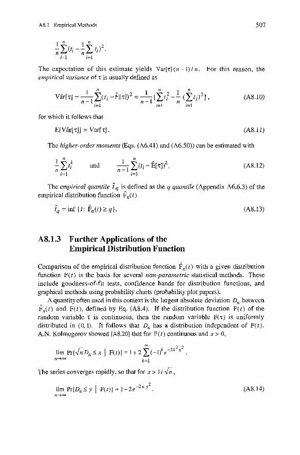
A8.1 Empirical Methods
The expectation of this estimate yields Var[c] (n - 1) l n . For this reason, the empirical variance of T is usually defined as
for which it follows that
E[V&[T]] = Var[z]
The higher-order moments (Eqs. (A6.41) and (A6.50)) can be estimated with
The empirical quantile F q is defined as the q quantile (Appendix A6.6.3) of the empirical distribution function ; , ( t )
fq = inf { t : F,(t) 2 q). (A8.13)
A8.1.3 Further Applications of the Empirical Distribution Function
Comparison of the empirical distribution function fi,(t) with a given distribution function F(t) is the basis for several non-parametric statistical methods. These include goodness-of-fit tests, confidence bands for distribution functions, and graphical methods using probability charts (probability plot papers).
A quantity often used in this context is the largest absolute deviation D, between ;,(t) and F(t) , defined by Eq. (A8.4). If the distribution function F( t ) of the random variable z is continuous, then the random variable F(T) is uniformly distributed in (0,l) . It follows that D, has a distribution independent of F(t). A.N. Kolmogorov showed [A8.20] that for F(t) continuous and X > 0,
m
k -2k2x2 iim &{&D, 5 x I F ( t ) ) = 1 + 2 E ( - l ) e n+- k=l
The series converges rapidly, so that for x > 1 / & ,
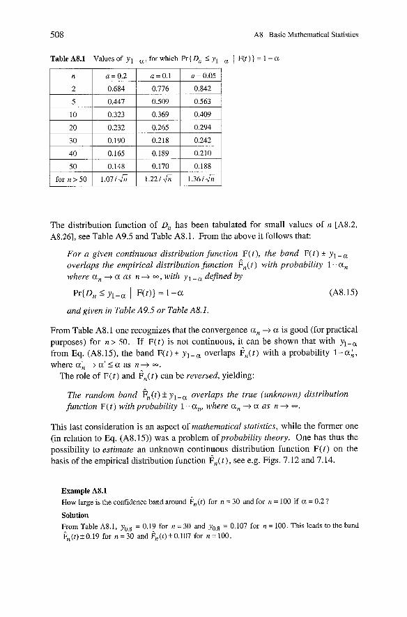
508 A8 Basic Mathematical Statistics
The distribution function of D,, has been tabulated for small values o A8.261, See Table A9.5 and Table A8.1. From the above it follows that:
For a given continuous distribution function F(t ) , the band F(t) + y l - , overlaps the empirical distribution function 6 J t ) with probability 1 -an where an + a as n + M, with y l - , defined by
Pr{Dn I yl-, I F(t)} = 1 -a (A8.15)
und given in Table A9.5 or Table A8.1.
From Table A8.1 one recognizes that the convergence an -+ a is good (for practical purposes) for n > 50. If F( t ) is not continuous, it can be shown that with yl-, from Eq. (A8.15), the band F(t) + yl - , overlaps 6,(t) with a probability 1 -an, w h e r e a i + a ' s a as n + m .
The role of F ( t ) and 6,(t) can be reversed, yielding: ..
The random band Fn(t)lt y l - , overlaps the true (unknown) distribution function F ( t ) with probability 1 - U„ where an -+ a as n + W.
This last consideration is an aspect of mathematical statistics, while the former one (in relation to Eq. (A8.15)) was a problem of probability theory. One has thus the possibility to estimate an unknown continuous distribution function F ( t ) on the basis of the empirical distribution function 6,(t) , see e.g. Figs. 7.12 and 7.14.
Example A8.1 How large is the confidence band around 6,(t) for n = 30 and for n = 100 if a = 0.2 ?
Solution From Table A8.1, y0,8 = 0.19 for n = 30 and y0.8 = 0.107 for n = 100. This leads to the band F,(t)10.19 for n=30 and Fn(t)f0.107 for n=100.
A8.1 Empirical Methods 509
To simplify investigations, it is often useful to draw 6,(t) on aprobability chart (probability plot paper). The method is as follows:
The empirical distribution function e , ( t ) is drawn in a system of coordinates in which a postulated type of continuous distribution function is represented by a straight liize; if the underlying distribution F ( t ) belongs to this type of distribution function, then for a sufficiently Zarge value of n the points ( t ( i ) , F,(t($) will approximate to a straight line (a systematic deviation from a straight line, particularly in the domain 0.1 < e,(t) < 0.9, leads to rejection of the type of distribution function assumed).
This can also be used as a simple rough visual check as to whether an assumed model ( F ( t ) ) seems correct. In many cases, estimates for unknown parameters of the underlying distribution function F ( t ) can be obtained from the estimated straight line for e,(t) . Probability charts for the Weibull (including exponential), lognormal and normal distribution functions are given in Appendix A9.8, some applications are in Section 7.5. The following is a derivation of the Weibull probability chart. The function
~ ( t ) = 1 - e-@t) P
can be transformed to loglo(l /(I - F(t))) = (At) loglo(e) and finally to
In the system of coordinates loglo(t) and loglo loglo(l l ( 1 - F( t ) ) , the Weibull distribution function given by ~( t )=l -e - (" ) ' appears as a straight line. Fig. A8.2 shows this for ß = 1.5 and h = 1 / 800 h . As illustrated by Fig. A8.2, the parameters ß and 3L can be obtained graphically
ß is the dope of the straight line, it appears on the scale loglo loglo(l / ( 1 - F(t)) if t is changed by one decade (e.g. from 102 to 103 in Fig. A8.2), for loglo loglo(l / ( 1 - F(t)) = loglo loglO(e), i.e. on the dashed line in Fig. A8.2, one has loglo(h t ) = 0 and thus h = 1 / t .
The Weibull probability chart also applies to the exponential distribution (P = 1). For a three parameter Weibull distribution (F( t ) = 1 - e-(h(t- 'v))ß, t V) one
can operate with the time axis t '= t - W , giving a straight line as before, or consider the concave curve obtained when using t (see Fig. A8.2 for an example). Conversely, from a concave curve describing a Weibull distribution (e.g. in the case of an empirical data analysis) it is possible to find W using the relationship
2 W = ( t l t2 - t M ) / ( t l + t2 - 2t, ) existing between two arbitrary points tl , t2 and t , obtained from the mean of F ( t l ) and F ( t 2 ) on the scale loglologlo(l / ( 1 - F(t)) ) , see Example A6.14 for a derivation and Fig. A8.2 for an application with tl=400h and t2 =1000h, yielding t,= 600h and ~ = 2 0 0 h .
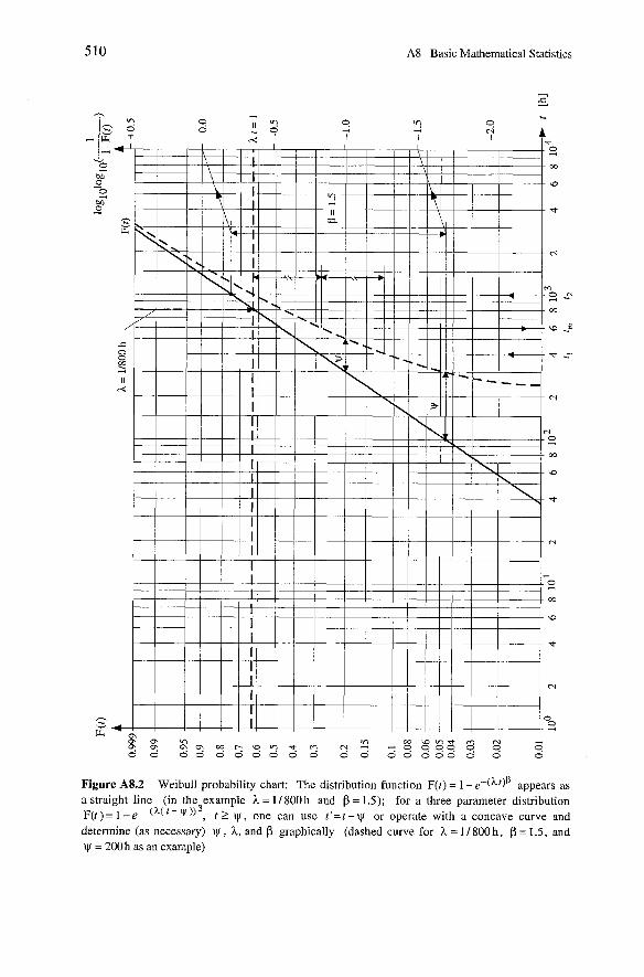
A8 Basic Mathematical Statistics
Figure A8.2 Weibull probability chart: The distribution function F(t) = 1 - e-(ht)P appears as a straight line (in the example h = 11 800 h and ß = 1.5); for a three Parameter distribution F@)= 1 - e - ( h ( t - v ) ) P , t 2 W , one can use t t=t-W or operate with a concave curve and determine (as necessary) W , h, and ß graphically (dashed curve for h = 1/800 h , ß = 1.5, and
= 200h as an example)
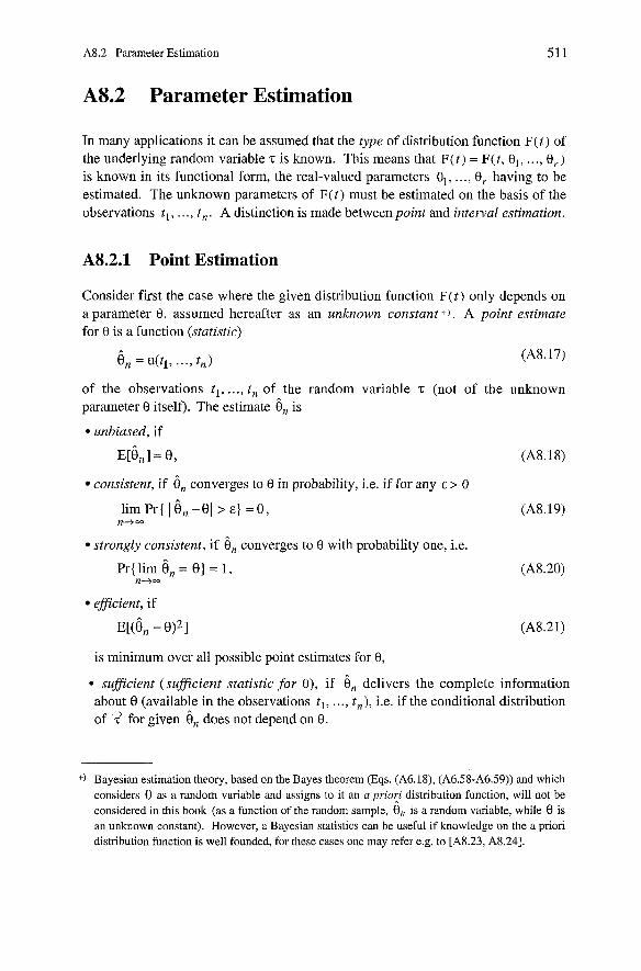
A8.2 Parameter Estimation
A8.2 Parameter Estimation
In many applications it can be assumed that the type of distribution function F ( t ) of the underlying random variable 2: is known. This means that F ( t ) = F(t, 01, ..., 0,) is known in its functional form, the real-valued parameters 01, . . ., 9, having to be estimated. The unknown Parameters of F( t ) must be estimated on the basis of the observations t l , ..., t,. A distinction is made betweenpoint and intewal estimation.
A8.2.1 Point Estimation
Consider first the case where the given distribution function F ( t ) only depends on a parameter 9, assumed hereafter as an unknown constant + ) . A point estimate for 9 is a function (statistic)
6 , = ~ ( t ~ , . . . , t,) (A8.17)
of the observations t l , ..., t , of the random variable T (not of the unknown parameter 9 itself). The estimate 6, is
unbiased, if
consistent, if 6, converges to 8 in probability, i.e. if for any E > 0
strongly consistent, if 6, converges to 0 with probability one, i.e.
efficient, if
E[(&, - fN2 I
is minimum over all possible point estimates for 9,
sufficient (sufficient statistic for B), if 6, delivers the complete information about 8 (available in the observations t l , ..., t,), i.e. if the conditional distribution of for given 6, does not depend on 9.
+) Bayesian estimation theory, based on the Bayes theorem (Eqs. (A6.18), (A6.58-A6.59)) and which considers 9 as a random variable and assigns to it an a priori distribution function, will not be considered in this book (as a function of the random sample, 0, is a random variable, while 0 is an unknown constant). However, a Bayesian statistics can be useful if knowledge on the a prion distnbution function is well founded, for these cases one may refer e.g. to [A8.23, A8.241.
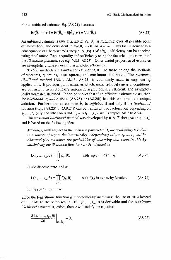
512 A8 Basic Mathematical Statistics
For an unbiased estimate, Eq. (A8.21) becomes
An unbiased estimate is thus efficient if ~ar[6,] is minimum over all possible point estimates for 8 and consistent if ~ar[6,] + 0 for n -+ =J. This last Statement is a consequence of Chebyschev's inequality (Eq. (A6.49)). Efficiency can be checked using the Cramkr - Rao inequality and sufficiency using the factorization criterion of the likelihood function, see e.g. [A8.1, A8.231. Other useful properties of estimates are asymptotic unbiasedness and asymptotic efficiency.
Several methods are known for estimating 8. To these belong the methods of moments, quantiles, least Squares, and maximum likelihood. The maximum likelihood method [A8.1, A8.15, A8.231 is commonly used in engineering applications. It provides point estimates which, under relatively general conditions, are consistent, asymptotically unbiased, asymptotically efficient, and asymptot- ically normal-distributed. It can be shown that if an efficient estimate exists, then the likelihood equation (Eqs. (A8.25) or (A8.26)) has this estimate as a unique solution. Furthermore, an estimate 6, is suficient if and only if the likelihood function (Eqs. (A8.23) or (A8.24)) can be written in two factors, one depending on t l , ..., t , only, the other on 8 and 6, = u(tl ,..., t,), see Examples A8.2 to A8.4.
The maximum likelihood rnethod was developed by R.A. Fisher [A8.15 (1921)l and is based on the following idea:
Maximize, with respect to the unknown Parameter 8 , the probabili~ (Pr) that in a sample of size n, the (statistically independent) values t l , ..., t , will be obsewed (i.e. maximize the probability of observing that record); this by maximizing the likelihoodfunction (L - Pr), defined as
in the discrete case, and as
n
L(tl, .. ., t„8) = n f ( t i , O ) , with f(ti, 0) as density function, (A8.24) i=l
in the continuous case.
Since the logarithmic function is monotonically increasing, the use of ln(L) instead of L leads to the same result. If L(tl , . . ., t„ 8 ) is derivable and the maximum likelihood estimate 6 , exists, then it will satisfy the equation
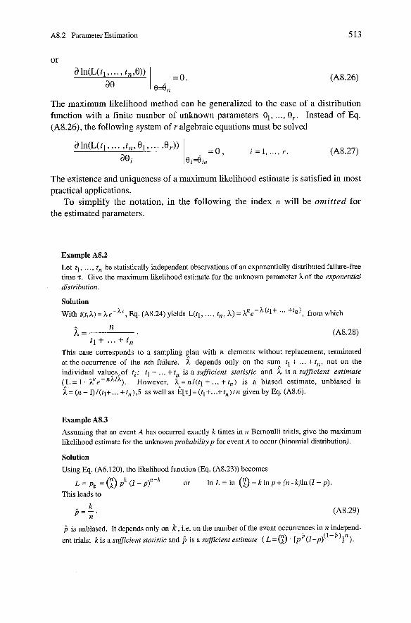
A8.2 Parameter Estimation 513
The maximum likelihood method can be generalized to the case of a distribution function with a finite number of unknown parameters 81, ..., 0,. Instead of Eq. (A8.26), the following system of r algebraic equations must be solved
The existence and uniqueness of a maximum likelihood estimate is satisfied in most practical applications.
To simplify the notation, in the following the index n will be omitted for the estimated parameters.
Example A8.2
Let t l , . . ., t, be statistically independent observations of an exponentially distnbuted failure-free time T. Give the maximum likelihood estimate for the unknown Parameter h of the exponential distribution.
Solution
With f(t, h ) = h e-" , Eq. (A8.24) yields L(tl, . . . , tn, h) = hne-h(tlt "' + ',), from which
This case corresponds to a sampling plan with n elements without replacement, terminated at the occurrence of the nth failure. h depends only on the sum t l + ... +t„ not on the individual values.of ti; tl + ... + tll is a sufficient statistic and ?L is a sufficient estimate (L = 1 hne-nh'h). However, h = nl(t l + ... + t,) is a biased estimate, unbiased is h= ( n - l)I(tl+ ... +t,),5 as weil as E[TI =(tl+ ...+ t , ) /n given by Eq. (A8.6).
Example A8.3
Assuming that an event A has occurred exactly k times in n Bernoulli trials, give the maximum likelihood estimate for the unknownprobabilityp for event A to occur (binomial distribution).
Solution
Using Eq. (A6.120), the likelihood function (Eq. (A8.23)) becomes
L = pk = (nk) pk (I - p)n-k or I n L = l n ( ~ ) + k l n p + ( n - k ) l n ( ~ - p ) . This leads to
j is unbiased. It depends only on k , i.e. on the number of the event occurrences in n independ-
ent trials; k is a suficient statistic and j is a suflcient estimate ( L=Q . [pe(l-p)(l-e)]n).
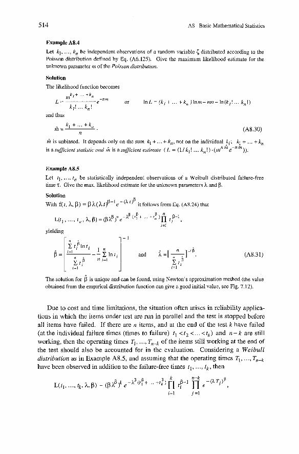
5 14 A8 Basic Mathematical Statistics
Example A8.4
Let kl, . . . , kn be independent observations of a random variable 5 distnbuted according to the Poisson distribution defined by Eq. (A6.125). Give the maximum likelihood estimate for the unknown Parameter m of the Poisson distribution.
Solution
The likelihood function becomes k l + ... + k , m
L = -nm or l n L = ( k , + ...+ k,)lnm-mn-In(kl! ... k,!) k*! ... kn!
and thus
f i is unbiased. It depends only on the sum kl + . . . + kn, not on the individual ki ; kl + . . . + k, is a suficient statistic and f i is a suficient estimate ( L = (1 / kl ! . . . kn !) . (mn e-n M)).
Example A8.5
Let tl, . . . , tn be statistically independent observations of a Weibull distributed failure-free time T. Give the max. likelihood estimate for the unknown Parameters h and P.
Solution B
With f(t, L, ß) = ß L ( L t)'-'e - " it follows from Eq. (A8.24) that
yielding
The solution for ß is unique and can be found, using Newton's approximation method (the value obtained from the empincal distribution function can give a good initial value, see Fig. 7.12).
Due to cost and time limitations, the situation often arises in reliability applica- tions in which the items under test are run in parallel and the test is stopped before all items have failed. If there are n items, and at the end of the test k have failed (at the individual failure times (times to failure) tl < t2 < . . . < tk) and n - k are still working, then the operating times Tl , ..., of the items still working at the end of the test should also be accounted for in the evaluation. Considering a Weibull distribution as in Example A8.5, and assuming that the operating times Tl, ..., Tnek have been observed in addition to the failure-free times tl , . . . , tk , then
ß ß k n-k (?JjP L ( I ~ , ..., tk, L, 0) - ( ß a ß f e - k ( t l + .., +ti)n t f - l e- ,
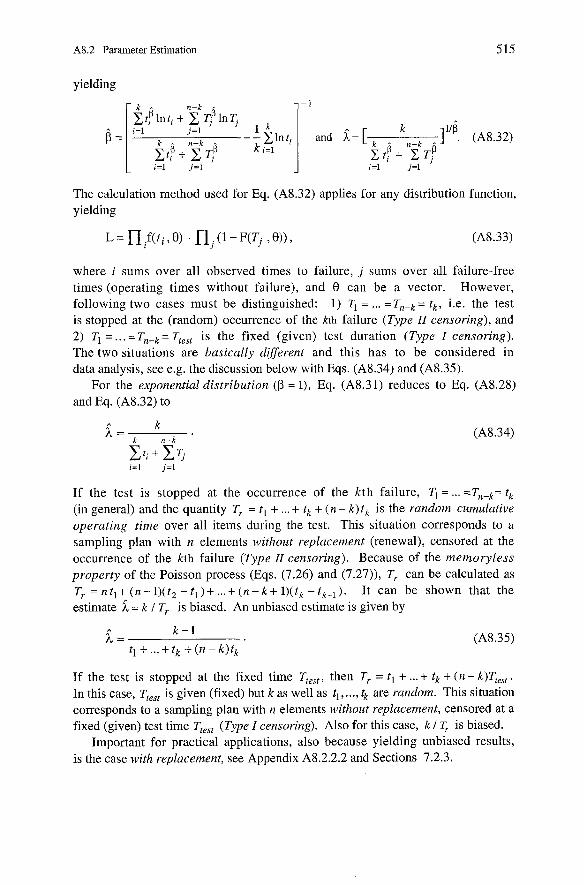
A8.2 Parameter Estimation
yielding
The calculation method used for Eq. (A8.32) applies for any distribution function, yielding
where i sums over all observed times to failure, j sums over all failure-free times (operating times without failure), and 8 can be a vector. However, following two cases must be distinguished: 1) Tl = ... = = tk, i.e. the test is stopped at the (random) occurrence of the kth failure (Type II censoring), and 2) Tl = . . . = = T„„ is the fixed (given) test duration (Type I censoring). The two situations are basically different and this has to be considered in data analysis, see e.g. the discussion below with Eqs. (A8.34) and (A8.35).
For the exponential distribution (P = I), Eq. (A8.31) reduces to Eq. (A8.28) and Eq. (A8.32) to
If the test is stopped at the occurrence of the k th failure, Tl = ... tk (in general) and the quantity T, = tl + ... + tk + (n - k)t, is the random cumulative operating time over all items during the test. This situation corresponds to a sampling plan with n elements without replacement (renewal), censored at the occurrence of the kth failure (Type II censoring). Because of the memoryless property of the Poisson process (Eqs. (7.26) and (7.27)), T, can be calculated as T, = n tl + (n - l)(t2 - tl ) + ... + (n - k + l)(tk - tk-l ). It can be shown that the estimate = k / T, is biased. An unbiased estimate is given by
If the test is stopped at the fixed time T„„, then T, = tl + ... + tk + (n - k)Ttest. In this case, T„, is given (fixed) but k as well as tl, ..., tk are random. This situation corresponds to a sampling plan with n elements without replacement, censored at a fixed (given) test time T„„ (Type I censoring). Also for this case, k / T, is biased.
Important for practical applications, also because yielding unbiased results, is the case with replacement, see Appendix A8.2.2.2 and Sections 7.2.3.
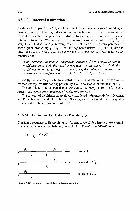
516 A8 Basic Mathematical Statistics
A8.2.2 Interval Estimation
As shown in Appendix A8.2.1, a point estimation has the advantage of providing an estimate quickly. However, it does not give any indication as to the deviation of the estimate from the true parameter. More information can be obtained from an interval estimation. With an intewal estimation, a (random) interval [ G 1 , G,] is sought such that it overlaps (covers) the true value of the unknown parameter 8 with a given probability y. [ G l , G,] is the confidence intenial, and 6 , are the lower and upper confidence limits, and y is the confidence level. y has the following interpretation:
In an increasing number of independent samples of size n (used to obtain confidence intewals), the relative frequency of the cases in which the confidence intewals [ G 1 , G,] overlap (cover) the unknown parameter 0 converges to the confidence level y = 1 - ßl - ß2 (0 < Pi .: 1 - ß2 < 1) .
ß, and ß, are the error probabilities related to the interval estimation. If y can not be reached exactly, the true overlap probability should be near to, but not less than, y.
The confidence interval can also be one-sided, i.e. (0, G,] or [ G l , W) for 8 r 0. Figure A8.3 shows some examples of confidence intervals.
The concept of confidence intervals was introduced independently by J. Neyman and R. A. Fisher around 1930. In the following, some important cases for quality control and reliability tests are considered.
A8.2.2.1 Estimation of an Unknown Probability p
Consider a sequence of Bernoulli trials (Appendix A6.10.7) where a given event A can occur with constant probability p at each trial. The binomial distribution
, B2 P1 C@ two-sided
0 81 e u
ßi 8 one-sided 6 I 6, 0
e u
, B2 0
~0 one-sided 6 2 el ei
Figure A8.3 Examples of confidence intervals for 0 2 0
A8.2 Parameter Estimation 517
gives the probability that the event A will occur exactly k times in n independent trials. From the expression for pk, it follows that
k2
Pr{kl 5 observations of A in n trials < k2 I p ) = (Y) pi( l - i=k,
However, in mathematical statistics, the Parameter p is unknown. A confidence intewal for p is sought, based on the observed number of occurrences of the event A in n Bernoulli trials. A solution to this problem has been presented by Clopper and Pearson [A8.6]. For given y = 1 - ß1 - ß2 ( 0 i ß, < 1 - P, < 1) the following holds:
I f in n Bemoulli trials the event A has occurred k tirnes, there is a probability nearly equal to (but not smaller than) y = 1 - ß1 - ß2 that the confidence inter- val [ F , , F , ] overlaps the true (unknown) probability p, with P1 & F , given by
c( l )p ; ( l - P,)"-' = ß 2 , for 0 < k < n , i=k
for k = 0 take
Pl=O and $ , = l - 6 , with y = 1 -P„ (A8.39)
und for k = n take
jl = and Pu = 1, with y =1-P,.
Considering that k is a random variable, P1 and P, are random variables. According to the footnote on p. 504, it would be more correct (from a mathematical point of view) to compute from Eqs. (A8.37) and (A8.38) the quantities pkl and pku, and then to set PI = pkl and P, = pku. For simplicity, this has been omitted here. Assuming p as a random variable, ß1 and ß2 would be the probabilities forp to be greater than and smaller than p l , respectively (Fig. A8.3).
The proof of Eqs. (A8.37) is based on the monotonic property of the function
For given (fixed) n, B, (k, p) decreases in p for fixed k and increases in k for fixed p (Fig. A8.4). Thus, for any p > 3, it follows that
B,(k,p)< B,(k,P,)=ß1.
For p > F „ the probability that the (random) number of observations in n trials will
A8 Basic Mathematical Statistics
Figure A8.4 Binomial distribution as a function of p for n fixed and two values of k
take one of the values O,1, . . ., k is thus < ßl (for p > p ' in Fig. A8.4, the Statement would also be true for a K > k). This holds in particular for a number of observations equal to k and proves Eq. (A8.38). Proof of Eq. (A8.37) is similar.
To determine pl and j, as in Eqs. (A8.37) and (A8.38), a Table of the Fisher distribution (Appendix A9.4) or of the Beta function can be used. However, for Pi = ß2 = (1 - Y ) / 2 and n sufficiently large, one of the following approximate solutions can be used in practical applications:
1. For large values on n (min(np , n(1- P ) ) > 5 ) , a good estimate for jl and j, can be found ushg the integral Laplace theorem. Rearranging Eq. (A6.149) and considering = k and ( k I n - instead of ( k I n - p ) yields
i=l
The right-hand side of Eq. (A8.41) is equal to the confidence level y , i.e.
Thus, for a given y , the value of b can be obtained from a table of the normal distribution (Table A9.1). b is the 1 - (1 - y ) 12 = ( I + y ) I 2 quantile of the standard normal distribution @ ( t ) , i.e., b = t (l+y),2 giving e.g. b = 1.64 for y = 0.9. On the left-hand side of Eq. (A8.41), the expression
is the equation of the confidence ellipse. For given values of k , n, and b,
A8.2 Parameter Estimation
confidence lirnits Pl and f i p n be determined as roots of Eq. (A8.42)
see Figs. A8.5 and 7.1 for some Examples.
2. For small values of n, confidence limits can be determined graphically from the envelopes of Eqs. (A8.37) and (A8.38) for ß1 = ß2 = (1 -Y) 1 2 , see Fig. 7.1 for y = 0.8 and y = 0.9. For n > 50, the curves of Fig. 7.1 practically agree with the confidence ellipses given by Eq. (A8.43).
One-sided confidence intewals can also be obtained from the above values for jl and F,. Figure A8.3 shows that
O l p < & , w i t h y = l - ß , and j l l p l l , w i t h y = l - ß 2 . (A8.44)
Example A8.6 Using confidence ellipses, give the confidence interval [jl, ju] for an unknown probability p for the case n = 50, k = 5, and y = 0.9.
Solution Setting n = 50, k = 5 , and b = 1.64 in Eq. (A8.43) yields the confidence interval [0.05, 0.191, see also Fig. 8.5 or Fig. 7.1 for a graphical solution. Corresponding one-sided confidence intervals would be p 1 0.19 or p 2 0.05 with y = 0.95.
Figure A8.5 Confidence limits (ellipses) for an unknown probability p with a confidence level y = 0.9 and for n = 10,25,50, 100 (according to Eq. (A8.43))
520 A8 Basic Mathematical Statistics
The role of kln and p in Eq. (A8.42) can be reversed, and Eq. (A8.42) can be used to solve a problem of probability theory, i.e. to compute for a given probability y , y = 1 - ßl - ß2 with ßl = ß2 , the limits kl and k2 of the number of observations k in n independent trials for given (fixed) values of p and n (e.g. the number k of defective items in a sample of size n)
As in Eq. (A8.43), the quantity b in Eq. (A8.45) is the (1+ y ) / 2 quantile of the normal distribution (e.g. b = 1.64 for y = 0.9 from Table A9.1). For a graphical solution, Fig. A8.5 can be used, taking the ordinatep as known and by reading kl In and k2 In from the abscissa. An exact solution follows from Eq. (A8.36).
A8.2.2.2 Estimation of the Parameter hfor an Exponential Distribution: Fixed Test Duration, with Replacement
Consider an item having a constant failure rate h and assume that at each failure it will be immediately replaced by a new, statistically equivalent item, in a negligible replacement time (Appendix A7.2). Because of the memoryless property (constant failure rate), the number of failures in (0, T1 is Poisson distributed and given by Pr{k failures in ( o , T ] I h ] = ( h ~ f e - ' T 1 k ! (Eq (A7.41)). The maximum likelihood point estimate for h follows from Eq. (A8.30), with n = 1 and m = AT, as
Similarly, estimation of the confidence interval for the failure rate h can be reduced to the estimation of the confidence intewal for the Parameter m = h T of a Poisson distribution. Considering Eqs. (A8.37) and (A8.38) and the similarity between the binomial and the Poisson distribution, the confidence limits and h, can be determined for given ßl, ßL, and y = 1 - ßl - ß2 ( 0 < Pi < i - ß2 < 1) from
and
for k = 0 takes
On the basis of the known relationship to the chi-square ( X 2 ) distribution
A8.2 Parameter Estimation 521
(Eqs. (A6.102), (A6.103), Appendix A9.2), the values hl and h, from Eqs. (A8.47) and (A8.48) follow from the quantiles of the chi-square distribution, yielding
0
for k > O , (A8.50)
ßl = ß2 = (1 - y ) / 2 is frequently used in practical applications. Fig. 7.6 gives the results obtained from Eqs. (A8.50) and (A8.51) for ß1 = ß2 = ( 1 - y ) / 2 .
One-sided confidence intewals are given as in the previous section by *
0 I h I h„ with y = 1 - ßl and hl I ?L < W, with y = 1 - ß2. (A8.52)
The situation considered by Eqs. (A8.47) to (A8.51) corresponds also to that of a sampling plan with n elements with replacement, each of them with failure rate h'= h l n , terminated at a fixed test time T„, = T. This situation is statistically different from that presented by Eq. (A8.34) and in Section A8.2.2.3.
A8.2.2.3 Estimation of the Parameter k for an Exponential Distribution: Fixed Number n of Failures, no Replacement
Let zl , ..., T , be independent random variables distributed according to a common distribution function F(t) = P ~ { T ~ 5 t ) = 1-e-", i = 1, ..., n. From Eq. (A7.39),
Setting a = n ( 1 - E ~ ) / h and b = n ( l + q)/ h it follows that
Considering now TI, ..., T, as a random sample of z with t l , ..., t , as observations, Eq. (A8.54) can be used to compute confidence limits il and i, for the parameter h. For given ßl, ß2 , and y = 1 - ßl - ß2 (0 i ß, < 1 - ß, < I), this leads to
h1 = ( I - E * ) ~ and h, = ( l + ~ ~ ) h , (A8.55)
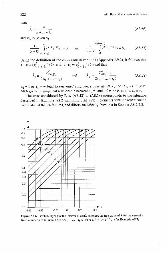
522 A8 Basic Mathematical Statistics
with * n h =
tl + ... +tn
and given by
Using the definition of the chi-square distribution (Appendix A9.2), it follows that )/Zn andthus ) /2n and ~ - E ~ = ( x ~ ~ , ~ ~ 1+ E1 = ( X z n , l -ß i
.. xLn , p, Al = and h,=
2(tl + ... +tn) 2(tl + ... +tn)
E2 = 1 or = 00 lead to one-sided confidence intervals [0, L,] or [ L l , W). Figure A8.6 gives the graphical relationship between n, y , and E for the case = = E.
The case considered by Eqs. (A8.53) to (A8.58) corresponds to the situation described in Example A8.2 (sampling plan with n elements without replacement, terrninated at the nth f ahre ) , and differs statistically from that in Section A8.2.2.2.
case of a A8.7)
Y
1.0 0.8
0.6
0.4
0.2
0.1 0.08
0.06
0.04
0.02
0.01 0.01 0.02 0.05 0.1 0.2 0.5
Figure A8.6 Probability 'y $at the interval (1 f c ) i overlaps the true value of h for the fixednumbernoffailures ( h = n l ( t l + ...+ t n ) , P r { ~ < t ] = l - e - ' ~ , *forExample
/
b E
A8.2 Parameter Estimation 523
Example AS.7
For the case considered by Eqs. (A8.53) to (A8.58), give for n = 50 and y = 0.9 the-two-sided confidence interval for the parameter h of an exponential distnbution as a function of h . Solution From Figure A8.6, E = 0.24 yielding the confidence interval [0.76h, 1.24 h] .
A8.2.2.4 Avaiiability Estimation (Erlangian Failure-Free and Repair Times)
Considerations of Section A8.2.2.3 can be extended to estimate the availability of a repairable item (described by the alternating renewal process of Fig. 6.2) for the case of Erlangian distributed failure-free andlor repair times (Appendix A6.10.3), and in particular for the case of constant failure and repair rates (exponentially distributed failure-free and repair times).
Consider a repairable item in continuous operation, new at t = 0 (Fig. 6.2), and assume constant failure and repair rates ( h ( x ) = h , p(x) = p). For this case, point and average unavailability converge rapidly ( 1-PAso(t) & 1-AAso( t ) in Table 6.3) to the asymptotic and steady-state value given by
h l ( h + p ) is a probabilistic value and has his statistical Counterpart in DT/(UT+DT), where DT is the down (repair) time and UT = t -DT the up (operating) time observed in (0 , t ] . To simplify considerations, it will be assumed in the following t >> MTTR = 1 I p (Table 6.3) and that at the time point t a repair is terminated and k failure-free and repair times have occurred ( k=1,2, ... ) . Furthermore, a«p, i.e.
- PA =1-PA = PA, = h / p (A8.59)
will be assumed here, yielding the counterpart DT I UT (relative error of magnitude PA). Considering that at the time point t a repair is terminated, it holds that
where ti & t i are the observed values of failure-free and repair times zi & T;, re- spectively. According to Eqs. (A6.102) - (A6.104), the quantity 2 h (zl +. . . +zk) has a ~2 distribution with V = 2 k degrees of freedom. The same holds for the repair times 2 y (7; + . . . +&J. From this, it follows (Appendix A9.4) that the quantity
is distributed according to a Fisher distribution (F) with v l = v 2 = 2 k degrees of freedom (E, is an unknown parameter, regarded here as a random variable)
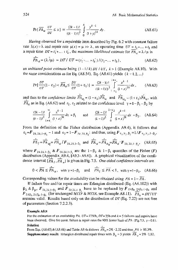
524 A8 Basic Mathematical Statistics
Having observed for a repairable item described by Fig. 6.2 with constant failure rate h(x) = h and repair rate p(x) = p >> h , an operating time UT = tl +. . . + tk and a repair time DT = t;+. . . + ti , the mmimum likelihood estimate for G, = h I p is
A
E , = ( k i P ) = D T I UT=( t i+ ...+ t i ) l ( t l + ...+ tk), (A8.62)
an unbiased point estimate being (1 - 1 I k) DT I U T , k r 1 (Example A8.10). With the same considerations as for Eq. (A8.54), Eq. (A8.61) yields ( k = i, 2, ...)
and thus to the confidence limits E,, = (1 - E 2 ) S a and sau = (1 + E ~ ) = ~ , with
2, as in Eq. (A8.62) and EI, related to the confidence level y = 1 - ß1 - ß2 by
(2k -I)! " xk-l (2k - I)! - j,dx=ß, and dx = P 2 . (A8.64) (k -1)12 (1 + X ) (k
From the definition of the Fisher distribution (Appendix A9.4), it follows that E I = F ~ ~ , ~ ~ , J - P , - 1 and E2= 1 - F 2 k , 2 k , ~ z ; andthus, using F v , , v 2 , ~ 2 = l l F v , , v , , ~ - ~ 2 ,
where F2k,2k,,-ß2 & F2k,2k,l-ß, are the 1 - ß2 & 1 - ßl quantiles of the Fisher ( F )
distribution (Appendix A9.4, [A9.3- A9.61). A graphical visualization of the confi- dence interval [G , ,] is given in Fig. 7.5. One-sided confidence intervuls are
,. - O < P A < P A „ withy=l-P, and Pal < % < I , withy=l-P,. (A8.66)
Corresponding values for the availability can be obtained using PA = 1 - X. If failure free andlor repair times are Erlangian distributed (Eq. (A6.102)) with
ßh & ßp, F2k,2k,l-ß2 and F 2k,2k,~-ß1 have to be replaced by F 2kßP .zkßh.l-ß2 and F2 k P h , 2 kPp (for unchanged MTTF & MlTR, See Exarnple A8.11). Ga = DT/ UT remains valid. Results based only on the distribution of DT (Eq. 7.22) are not free of parameters (Section 7.2.2.3).
Example A8.S For the estimation of an availability PA, UT= 1750h, DT= 35h and k= 5 failures and repairs have been observed. Give for const. failure & repair rates the 90% lower limit of PA (Fig.7.5, y = 0.8).
Solution From Eqs. (A8.65) & (A8.66) and Table A9.4a follows zu = 2%. 2.32 and thus -PA > 95.3%. Supplementary result: Erlangian distributed repair times with PP = 3 yields E, = 2% .1.82.
A8.3 Testing Statistical Hypotheses
A8.3 Testing Statistical Hypotheses
When testing a statistical hypothesis, the objective is to solve the following problem:
From one's own experience, the nature of the problem, or simply as a basic hypothesis, a specific null hypothesis Ho is formulated for the statistical properties of the obsewed random variable; sought is a rule which allows rejection or acceptance of Ho on the basis of the statistically independent ob- sewations made from a sample of the random variable under consideration .
If R is the unknown reliability of an item,following null hypotheses Ho are possible:
la) Ho: R = 4 Ib) H,: R > & lc) Ho: R < & .
To test whether the failure-free time of an item is distributed according to an exponential distribution Fo(t) = 1 - e - X with unknown h, or Fo(t) = 1 - e - with known ko , the following null hypotheses Ho can be for instance formulated:
2a) Ho : the distribution function is Fo(t)
2b) Ho : the distribution function is different from Fo(t)
2c) Ho : h = hO, provided the distribution is exponential
2d) Ho : h < ho, provided the distribution is exponential 2e) Ho : the distribution function is 1 - e-ht , Parameter h unknown.
It is usual to subdivide hypotheses into parametric (la, lb, lc, 2c, 2d) and non- parametric ones (2a, 2b, and 2e). For each of these types, a distinction is also made between simple hypotheses (la, 2a, 2c) and composite hypotheses ( lb , lc, 2b, 2d, 2e). When testing a hypothesis, two kinds of errors can occur (Table A8.2):
type I error, i.e. the error of rejecting a true hypothesis Ho, the probability of this error is denoted by a type II error, i.e. the error of accepting a false hypothesis Ho, the probability of this error is denoted by ß (to compute ß, an alternative hypothesis H1 is necessary, ß is then the probability of accepting Ho assuming H1 is true).
If the sample space is divided into two complementary sets, A for acceptance and 3 for rejection, the type I and type I1 errors are given by
a = Prisample in 3 I H o true},
ß = Pr{sample in A I Ho false (Hi true)}.
Both kinds of error are possible and cannot be minimized simultaneously. Often a
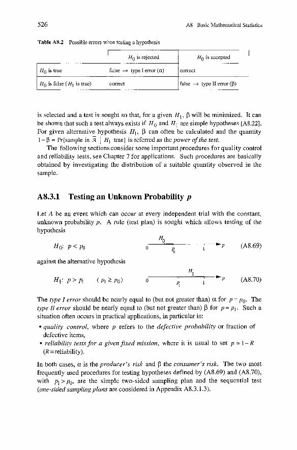
526 A8 Basic Mathematical Statistics
Table A8.2 Possible errors when testing a hypothesis
I HO is false ( H 1 is true) 1 correct I false + type I1 error (0) I Ho is true
is selected and a test is sought so that, for a given H 1 , ß will be minimized. It can be shown that such a test always exists if H o and H 1 are simple hypotheses [A8.22]. For given alternative hypothesis H1, ß can often be calculated and the quantity 1 - ß = Pr{sarnple in 3 I H1 true] is referred as the power of the test.
The following sections consider some important procedures for quality control and reliability tests, see Chapter 7 for applications. Such procedures are basically obtained by investigating the distribution of a suitable quantity observed in the sample.
A8.3.1 Testing an Unknown Probability p
Ho is rejected
false + type I error ( C X )
Let A be an event which can occur at every independent trial with the constant, unknown probability p . A rule (test plan) is sought which allows testing of the hypothesis
Ho: P < Po 0 1 )P (A8.69) Po
Ho is accepted
correct
against the alternative hypothesis
Hl HI: ~ > m ( ~ 1 2 ~ 0 1 o 1 (A8.70)
The type I error should be nearly equal to (but not greater than) a for p = po. The type II error should be nearly equal to (but not greater than) ß for p = pl. Such a situation often occurs in practical applications, in particular in:
quality control, where p refers to the defective probability or fraction of defective items, reliability tests for a given fixed mission, where it is usual to set p = 1 - R (R =reliability).
In both cases, a is the producer's risk and ß the consumer's risk. The two most frequently used procedures for testing hypotheses defined by (A8.69) and (A8.70), with pi >pO, are the simple two-sided sampling plan and the sequential test (one-sided sampling plans are considered in Appendix A8.3.1.3).
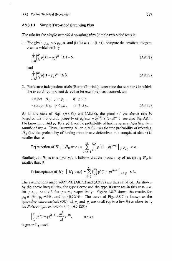
A8.3 Testing Statistical Hypotheses
A8.3.1.1 Simple Two-sided Sampling Plan
The rule for the simple two-sided sampling plan (simple two-sided test) is:
1. For given po, pl >po, a, and ß (0 < a < 1 - ß < I), compute the smallest integers C and n which satisfy
and
2. Perform n independent trials (Bernoulli trials), determine the number k in which the event A (component defective for example) has occurred, and
*reject Ho: p < p o , if k > c
accept Ho: p < po , if k 5 C.
As in the case of Eqs. (A8.37) and (A8.38), the proof of the above rule is based on the inonotonic property of Bn(c, p ) = k( Y) (I - see also Fig A8.4. For known n, C , and p, B,(c,p) gives the pobab?lity of having up to C defectives in a sample of size n. Thus, assuming H o true, it follows that the probability of rejecting H o (i.e. the probability of having more than C defectives in a sample of size n) is smaller than a
n Pr{rejection of H o / Ho true} = ( . ) p i ( l - "P' I Y < a ,
1 i=c+l
Similarly, if H1 is true ( p > p l ) , it follows that the probability of accepting Ho is smaller than ß
Pr{acceptanceof H o 1 Xi true) = 5 ("pi(i-p)"-i I < P . i=O
The assumptions made with Eqs. (A8.71) and (A8.72) are thus satisfied. As shown by the above inequalities, the type I error and the type I1 error are in this case < a for p < po and < ß for p> pl, respectively. Figure A8.7 shows the results for po = 1%, pl = 2%, and a = ß 220%. The curve of Fig. A8.7 is known as the operating characteristic (OC). If po and pl are small (up to a few %) or close to 1, the Poisson approximation (Eq. (A6.129))
is generally used.
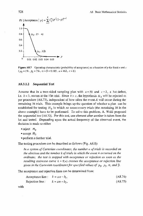
A8 Basic Mathematical Statistics
Pr {Acceptance 1 p ] = (f )P i ( l - ~ ~ i
4 i=O
Figure AS.7 Operating characteristic (probability of acceptance) as a function of p for fixed n and C
( p o = l % , p1 =2%, u=ß=0.185, n=462 , c = 6 )
A8.3.1.2 Sequential Test
Assume that in a two-sided sampling plan with n = 50 and C = 2 , a 3rd defect, i.e. k = 3, occurs at the 12th trial. Since k > C , the hypothesis H o will be rejected as per procedure (A8.73), independent of how often the event A will occur during the remaining 38 trials. This example brings up the question of whether a plan can be established for testing H o in which no unnecessary trials (the remaining 38 in the above example) have to be performed. To solve this problem, A. Wald proposed the sequential test [A8.32]. For this test, one element after another is taken from the lot and tested. Depending upon the actual frequency of the observed event, the decision is made to either
reject Ho
accept Ho
perform a further trial.
The testing procedure can be described as follows (Fig. A8.8):
Zn a system of Cartesian coordinates, the rzumber n of trials is recorded on the abscissa und the number k of trials in which the event A occurred on the ordinate; the test is stopped with acceptance or rejection as soon as the resulting staircase cuwe k = f(n) crosses the acceptance or rejection line given in the Cartesian coordinates for specified values of po, pi, a, und ß.
The acceptance and rejection lines can be determined from:
Acceptance line : k = an - bl,
Rejection line : k = an + b2,
with

A8.3 Testing Statistical Hypotheses
k
Figure A8.8 Sequential test for po = 1%, pl = 2%, and a = ß = 20%
W - P O ) / ~ ~ - P I ) ) in((1 - a ) /ß a =
m ]-PO i= P,
1 - Po ln((l-ß)'a . (A8.76) 1?= I?
In- + ln- In- + In-- ' - Po In-+In-
P, ] - P , Po ] - P , Po 1-f+
Figure A8.8 shows acceptance and rejection lines for po= 1%, pl= 2%, a = ß =20%. Practical remarks related to sequential tests are given in Sections 7.1.2.2 and 7.2.3.2.
AS.3.1.3 Simple One-sided Sampling Plan
In many practical applications only po and a or pl and ß are specified, i.e. one Want to test H o : P< po against H 1 : P> po with type I error a o r H o : p< pl against H 1 : p>pl with type I1 error P. In these cases, only Eq. (A8.71) or Eq. (A8.72) can be used and the test plan is a pair (C, n) for each selected value of C = 0, I,. . . and calculated value of n. Such plans are termed one-sided sampling plans.
Setting pl = po in the relationship (A8.70) or in other words, testing
H o : P C P 0 (A8.77)
against
H11 P > P o
with type I error a, i.e. using one (c,n) pair (for C = 0,1, ...) from Eq. (A8.71) and the test procedure (A8.73), the type I1 error can become very large and reach the value 1 - a for p = po. Depending upon the value selected for C = 0,1,. . . and that calculated for n (the smallest integer n which satisfies Eq. (A8.71)), different plans (pairs of (C, n)) are possible. Each of these plans yields different type I1 errors. Figure A8.9 shows this for some values of C (the type I1 error is the ordinate of the
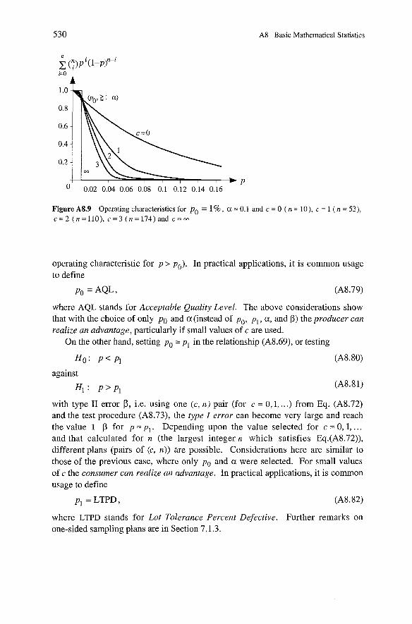
A8 Basic Mathematical Statistics
Figure A8.9 Operating characteristics for po = 1 %, a = 0.1 and C = 0 ( n = 10), C = 1 ( n = 53), c = 2 (n=110), c = 3 ( n = 1 7 4 ) a n d c = w
operating characteristic for p > po). In practical applications, it is common usage to define
where AQL stands for Acceptable Quality Level. The above considerations show that with the choice of only po and a(instead of po, p,, a, and ß) the producer can realize an advantage, particularly if small values of c are used.
On the other hand, setting po = p, in the relationship (A8.69), or testing
Ho: P < P1 (A8.80)
with type I1 error P, i.e. using one (C , n) pair (for C = 0,1, ...) from Eq. (A8.72) and the test procedure (A8.73), the type I error can become very large and reach the value 1 - ß for p = P,. Depending upon the value selected for C = 0,1, . . . and that calculated for n (the largest integer n which satisfies Eq.(A8.72)), different plans (pairs of ( C , n)) are possible. Considerations here are similar to those of the previous case, where only po and a were selected. For small values of C the consumer can realize an advantage. In practical applications, it is common usage to define
p, = LTPD, (A8. 82)
where LTPD stands for Lot Tolerance Percent Defective. Further remarks on one-sided sampling plans are in Section 7.1.3.
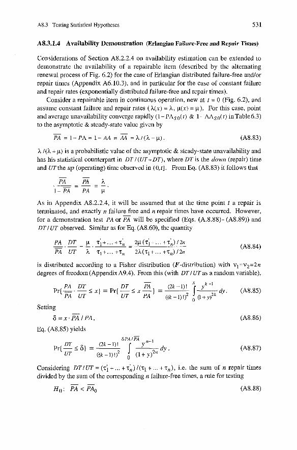
A8.3 Testing Statistical Hypotheses 531
AS.3.1.4 Availability Demonstration (Erlangian Faiiure-Free and Repair Times)
Considerations of Section A8.2.2.4 on availability estimation can be extended to demonstrate the availability of a repairable item (described by the alternating renewal process of Fig. 6.2) for the case of Erlangian distributed failure-free and/or repair times (Appendix A6.10.3), and in particular for the case of constant failure and repair rates (exponentially distributed failure-free and repair times).
Consider a repairable item in continuous operation, new at t = 0 (Fig. 6.2), and assume constant failure and repair rates ( h ( x ) = h, y(x) = P). For this case, point and average unavailability converge rapidly ( 1 - PA„( t ) & 1 - AAso( t ) inTable6.3) to the asymptotic & steady-state value given by
h / ( h + y ) is a probabilistic value of the asymptotic & steady-state unavailability and has his statistical Counterpart in DT I (UT+ DT), where DT is the down (repair) time and UT the up (operating) time observed in (O,t] . From Eq. (A8.83) it follows that
As in Appendix A8.2.2.4, it will be assumed that at the time point t a repair is terminated, and exactly n failure free and n repair times have occurred. However, for a demonstration test PA or will be specified (Eqs. (A.8.88)- (A8.89)) and DTl UT observed. Similar as for Eq. (A8.60), the quantity
is distributed according to a Fisher distribution (F-distribution) with v1=v2=2n degrees of freedom (Appendix A9.4). From this (with DT 1 UT as a random variable),
- dy. (A8.85)
PA UT
Setting
6 = x . P A ~ ~ ~ , Eq. (A8.85) yields
Considering DT I UT = (T; + . . . + T;) /(q + . . . + T ~ ) , i.e. the sum of n repair times divided by the sum of the corresponding n failure-free times, a rule for testing
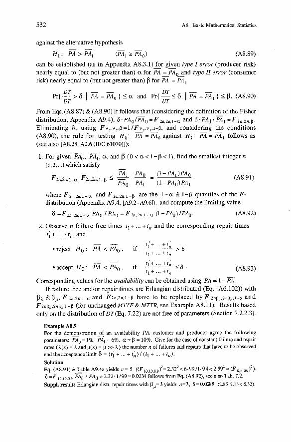
532 A 8 Basic Mathematical Statistics
against the alternative hypothesis
H1: &Xl ( P A , r P A o ) (A8.89)
can be established (as in Appendix A8.3.1) for given type I error (producer risk) nearly equal to (but not greater than) a for E = E, and type II error (consumer risk) nearly equal to (but not greater than) ß for E = E,
DT DT Pr(->i3 I E = E o } S a and Pr{-58 I PA = P A , } Iß. (A8.90)
UT UT
From Eqs. (A8.87) & (A8.90) it follows that (considering the definition of the Fisher distribution, Appendix A9.4), 6. P A ~ I P A ~ =F 2n,2n,1-a and 6. PA1 I PA1 = F 2n ,2n ,ß .
Eliminating F , using F v „ v „ =1 / F v „ v , , - B , and considering - - the conditions (A8.90), the rule for testing H o : PA = PAo against H , : PA = PA, follows as (see also [A8.28, A2.6 (IEC 61070)l):
1. For given %, q, a, and ß (0 < a < 1 - ß < I), find the smallest integer n (1,2, ...) which satisfy
where F 2,,, 2n, 1 - C L and F zn, zn, 1 - p are the 1 - a & 1 - ß quantiles of the F- distribution (Appendix A9.4, [A9.2-A9.6]), and compute the lirniting value
8 = F 2 n , z n , l - a /PAo = F 2 n , ~ n , l - ~ ( ~ - P ~ I ) I P ~ I . (A8.92)
2. Observe n failure free times tl + ... + t , and the corresponding repair times t ; + ... + t;, and
accept H~ : PA < PAo , Corresponding values for the availability can be obtained using PA = 1 - H.
If failure free and/or repair times are Erlangian distributed (Eq. (A6.102)) with ß h &Pp, F 2n,2n,l-a and F 2 n . z n , i - ß have to be replaced by F 2nß„~nßh , l -a and F2nßh,2nß„l - ß (for unchanged MTTF & MTTR, see Example A8.11). Results based only on the distribution of DT (Eq. 7.22) are not free of Parameters (Section 7.2.2.3).
Exarnple A8.9 For the demonstrationof - an availability PA, customer and producer agree the following Parameters: PAo = 1%, PAl = 6%, a = ß = 10%. Give for the case of constant failure and repair rates ( & ( X ) = h and ~ ( x ) = p >> h ) the number n of failures and repairs that have to be observed and the acceptance limit 6 = ( t i + ... + t ; ) 1 ( t l + ... + t , ) .
Solution Eq. (A8.91) & Table A9.4a yields n= 5 ( ( F i0,i0,0,9)2=2.322< 6 . 9 9 / 1 . 9 4 < 2.59'= ( F 8,8,09)2) . 6 = F „-„ .,,, PAo I PAO = 2.32.1199 =0.0234 follows from Eq. (A8.92), See also Tab. 7.2.
Suppl. result: Erlangian distr. repair times with ßp=3 yields n=3, 6= 0.0288 (2.85.2.13 < 6.32).
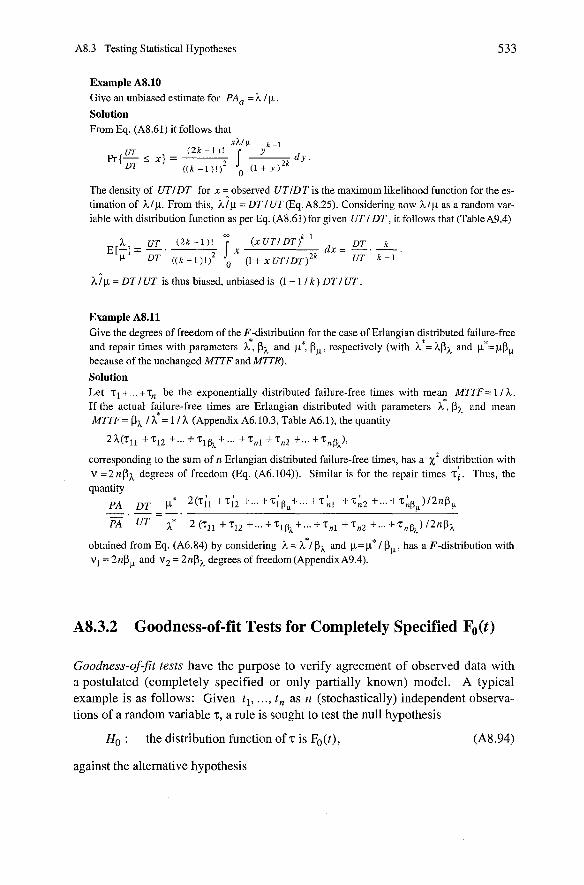
A8.3 Testing Statistical Hypotheses
Example A8.10 Give an unbiased estimate for PA, = h l p .
Solution From Eq. (A8.61) it follows that
xhlp UT ( 2 k - I ) ! y k -'
Pr(-<X]=--- - DT
d Y ( ( k - I ) ! ? ( 1 + J ' l z k
The density of UTIDT for X 7 observed UTIDT is the maximum likelihood function for the es- timation of Alp. From this, Alp = DTI UT (Eq. A8.25). Considenng now Alp as a random var- iable with distribution function as per Eq. (A8.61)for given UTI DT, it follows that (TableA9.4)
h i p = DT I UT is thus biased, unbiased is (1 - 1 I k ) DTI UT
Example A8.11 Give the degrees of freedom of the F*-distnbution for the case of Erlangian distributed failure-free and repair times with Parameters h , ßh and P*, ßP, respectively (with h f= hßh and pf= pßp because of the unchanged MTTF and MTTR).
Solution Let T I + ... +T, be the exponentially distributed failure-free times with mean MTTF= 1 I h . If the actual failure-free times are Erlangian distributed with parameters h*, ßh and mean MTTF= ßh lh*= 1 I h (Appendix A6.10.3, Table A6.1), the quantity
corresponding to the surn of n Erlangian distnbuted failure-free times, has a distnbution with V =2 nßh degrees of freedom (Eq. (A6.104)). Similar is for the repair times Ti. Thus, the quantity
PA DT 2(Ti1 +T;, +...+ T;~,+.. . +T:, -!-T;, +... + ~ ; ~ , ) / 2 n ß , _ . _ = - . - PA UT L* 2 (T„ + T„ +... + Tlph +... +T,] + T , ~ +... +T,&) 12nßh
obtained from Eq. (A6.84) by considering h =L*/ ßh and p=pf 1 PP, has a F-distribution with vl = 2 n ß , and V, = 2nßh degrees of freedom (AppendixA9.4).
AS.3.2 Goodness-of-fit Tests for Completely Specified F0(t)
Goodness-of-fit tests have the purpose to verify agreement of observed data with a postulated (completely specified or only partially known) model. A typical example is as follows: Given tl, . . ., t , as n (stochastically) independent observa- tions of a random variable T, a rule is sought to test the null hypothesis
Ho : the distribution function of T is Fo(t), (Ag. 94)
against the alternative hypothesis
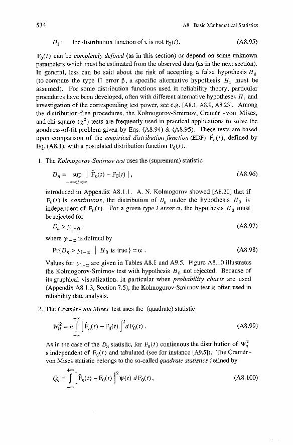
534 A8 Basic Mathematical Statistics
Hl : the distribution function of T is not Fo(t). (A8.95)
F,(t) can be completely defined (as in this section) or depend on some unknown parameters which must be estimated from the observed data (as in the next section). In general, less can be said about the risk of accepting a false hypothesis H, (to compute the type 11 error P , a specific alternative hypothesis H, must be assumed). For some distribution functions used in reliability theory, particular procedures have been developed, often with different alternative hypotheses H, and investigation of the corresponding test power, see e.g. [A8.l, A8.9, A8.231. Among the distribution-free procedures, the Kolmogorov-Smirnov, Cramkr -von Mises, and chi-square (X') tests are frequently used in practical applications to solve the goodness-of-fit problem given by Eqs. (A8.94) & (A8.95). These tests are based upon comparison of the empirical distribution function (EDF) G,(t), defined by Eq. (A8.1), with a postulated distribution function Fo(t) .
1. The Kolmogorov-Smirnov test uses the (supremum) statistic
introduced in Appendix A8.1. 1. A. N. Kolmogorov showed [A8.20] that if F,(t) is continuous, the distribution of D, under the hypothesis H, is independent of F,(t). For a given type I error a , the hypothesis H, must be rejected for
D, > Yl-W (A8.97)
where yl-, is defined by
Pr{Dn > yi-, I H, is true} = a . (A8.98)
Values for y ,-, are given in Tables A8.1 and A9.5. Figure A8.10 illustrates the Kolmogorov-Srnirnov test with hypothesis Ho not rejected. Because of its graphical visualization, in particular when probability charts are used (Appendix A8.1.3, Section 7.5), the Kolmogorov-Smirnov test is often used in reliability data analysis.
2. The Cramdr- von Mises test uses the (quadrate) statistic
-W
As in the case of the D, statistic, for Fo(t) continuous the distribution of W; s independent of F,(t) and tabulated (see for instance [A9.5]). The Cramer - von Mises statistic belongs to the so-called quadrate statistics defined by
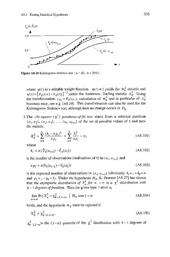
A8.3 Testing Statistical Hypotheses
Figure A8.10 Kolmogorov-Smimov test ( n = 20, a = 20%)
where ~ ( t ) is a suitable weight function. ~ ( t ) = 1 yields the W: statistic and ~ ( t ) = [F,(t) ( 1 - F,(t))] -' yields the Anderson- Darling statistic A:. Using the transformation z ( i ) = F,(t(i,), calculation of W: and in particular of A: becomes easy, see e.g. [A8.10]. This transformation can also be used for the Kolmogorov-Srnirnov test, although here no change occurs in D,.
3.The chi-square ( X 2 ) goodness-of-fit test starts from a selected partition ( a l , a 2 ] , ( a 2 , a g ] , .. ., ( a k , of the set of possible values of T and uses the statistic
is the number of observations (realizations of T) in ( a i , ai+l] and
is the expected number of observations in (a i , ai+l] (obviously kl +... + kk = n and pl +... +pk = 1 ) . Under the hypothesis H o , K. Pearson EA8.271 has shown that the asymptotic distribution of X: for n + is a X 2 distribution with k - 1 degrees of freedom. Thus for given type I error a ,
lim Prix: > x~-l,l-a 1 H o true } = (Y. (A8.104) n-f-
holds, and the hypothesis H o must be rejected if
is the ( 1 - a ) quantile of the X 2 distribution with k - 1 degrees of Xk-1,l-a
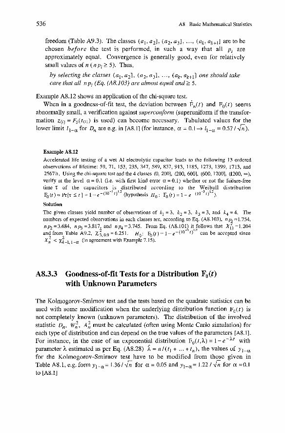
536 A8 Basic Mathematical Statistics
freedom (Table A9.3). The classes ( a l , a 2 ] , ( a 2 , a 3 ] , .. ., ( a k , ak+,] are to be chosen b e f o r e the test is performed, in such a way that all pi are approximately equal. Convergence is generally good, even for relatively small values of n (np i 2 5). Thus,
b y selecting the classes ( a l , a 2 ] , ( a 2 , a 3 ] , ..., ( a k , ak+l] one should take
care that all n p i (Eq. (A8.103) are almost equal und 1 5.
Example A8.12 shows an application of the chi-square test. When in a goodness-of-fit test, the deviation between 6, ( t ) and F o ( t ) seems
abnormally small, a verification against superconform (superuniform if the transfor- mation qi) = F o ( t ( i l ) is used) can become necessary. Tabulated values for the lower limit L I - , for D, are e.g. in [A8.1] (for instance, a = 0.1 -+ Z 1 - , = 0.57 I&).
Example A8.12 Accelerated life testing of a wet Al electrolytic capacitor leads to the following 13 ordered observations of lifetime: 59, 71, 153, 235, 347, 589, 837, 913, 1185, 1273, 1399, 1713, and 2567 h. Using the chi-square test and the 4 classes (0, 2001, (200, 6001, (600, 12001, (1200, M), verify at the level a = 0.1 (i.e. with first kind error a = 0.1) whether or not the failure-free time T of the capacitors is distributed according to the Weibull distribution Fo(t)=Pr{z < t ) = l - e - ( 1 0 - ~ t ) " ~ (hypothesis H o : F o ( t ) = l - e - ( l o J z ) ' . ~ ) ,
Solution The given classes yield number of observations of kl = 3, k2 = 3, k , = 3, and k4 = 4. The numbers of expected observations in each classes are, according to Eq. (A8.103), n p -1.754, 1 - np2 =3.684, np3 =3.817, and np4 =3.745. From Eq. (A8.101) it follows that X13 =1.204
2 -3 1.2 and from Table A9.2, X 3, 0.9 = 6.251. Ho : F. (t ) = 1 - e-(1° ') can be accepted since
2 2 X, < x ~ - ~ , -cx (in agreement with Example 7.15).
A8.3.3 Goodness-of-fit Tests for a Distribution F,,(t) with Unknown Parameters
The Kolmogorov-Smirnov test and the tests based on the quadrate statistics can be used with some modification when the underlying distribution function F,( t ) is not completely known (unknown parameters). The distribution of the involved statistic Dn, W;, A: must be calculated (often using Monte Carlo simulation) for each type of distribution and can depend on the true values of the parameters [A8.1]. For instance, in the case of an exponential distribution FO( t ,h ) = 1- e-nt with parameter ?L estimated as per Eq. (A8.28) h = n l ( t l + ... + t,), the values of Y , - ,
for the Kolmogorov-Smirnov test have to be modified from those given in TableA8.1,e.g.formyl-,=1.36/& for a=0 .05 and yl- ,=1.22/& for a = 0 . 1 to [A8.1]
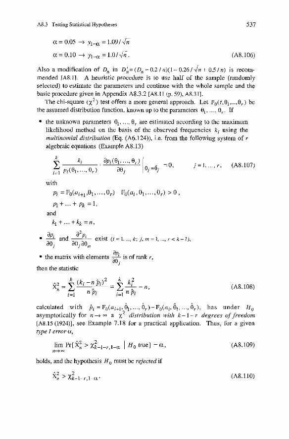
A8.3 Testing Statistical Hypotheses 537
Also a modification of D, in DA= (D,, - 0.2 / n)( l + 0.26 / & + 0.5 / n) is recom- mended rA8.11. A heuristic procedure is to use half of the sample (randomly selected) to estimate the parameters and continue with the whole sample and the basic procedure given in Appendix A8.3.2 [A8.11 (p. 59), A8.311.
The chi-square ( X * ) test offers a more general approach. Let Fo(t,B1, ..., B,) be the assumed distribution function, known up to the parameters e l , . . ., 8,. If
the unknown parameters 01, . . ., 8, are estimated according to the maximum likelihood method on the basis of the observed frequencies ki using the multinomial distribution (Eq. (A6.124)), i.e. from the following system of r algebraic equations (Example A8.13)
P1 + ... + pk = I ,
and kl + ... + kk = n ,
a ~ i a2pi exist (i = i, ..., k ; j, m = 1. .., r < k - I), - and - ae, ae, aem api
the matrix with elements - is of rank r, ae then the statistic
calculated with Pi = F , ( U ~ + ~ , i l , ..., 8,) - ~ ~ ( a ~ , GI, ..., G , ) , has under H , asymptotically for n -+ a x2 distribution with k - 1 - r degrees of freedom [A8.15 (1924)], see Example 7.18 for a practical application. Thus, for a given type I error a,
holds, and the hypothesis H, must be rejected if
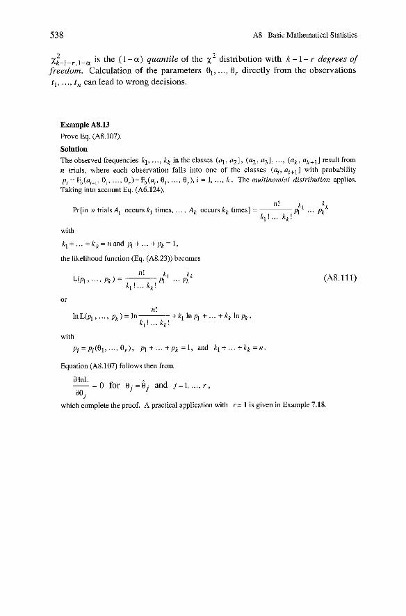
538 A8 Basic Mathematical Statistics
2 2 is the (1 - a ) quantile of the X distribution with k - 1 - r degrees of freedom. Calculation of the Parameters 01, . . ., 8 , directly from the observations t l , ..., tn can lead to wrong decisions.
Example A8.13
Prove Eq. (A8.107).
Solution The observed frequencies kl , ..., kk in the classes (al , a 2 ] , ( aZ , a j ] , . .., ( a k , ak+l] resuit from n trials, where each observation falls into one of the classes (ai , ai+l] with probability pi = F,,(a,+, , 8„ . .., e r ) - F, (a i , 8„ . . ., e r ) , i = 1, . . . , k . The multinomial distribution applies. Taking into account Eq. (A6.124),
n! k , k k Pr{in n trials Al occurs k, times, . . . , Ak occurs kk times) = - m ... pk
k l ! ... k k !
with
kl+ ...+ kk=nand m t . . .+pk= 1,
the likelihood function (Eq. (A8.23)) becomes
with
pi =pi(O1, ..., € I r ) , pl + ... +pk =1, and kl+ ... +kk = n
Equation (A8.107) follows then from
a lnL - = 0 for 8 . = B j and j = 1, ..., r , aej I
which complete the proof. A practical application with r = 1 is given in Example 7.18.
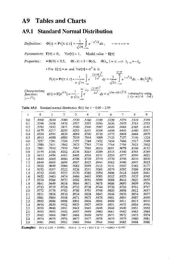
A9 Tables and Charts
A9.1 Standard Normal Distribution
Parameters: E[z] = 0 , Var[z] = 1, Modal value = E[z]
Properties: @ ( 0 ) = 0.5, t ) = 1 - ( t ) , @ ( t , ) = a => tl-, = - t ,
Table A9.1 Standard normal distribution @(t) for t = 0.00 - 2.99
Examples: Pr{r < 2.33) = 0.9901; p r { ~ < -1) = 1 - PI{T < 1 ) = 1 - 0.8413 = 0.1587
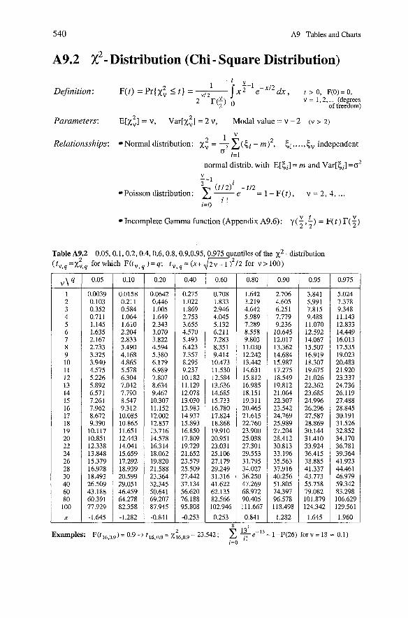
540 A9 Tables and Charts
A9.2 x2- Distribution (Chi - Square Distribution) t
Definition : F(t) = PI-{%; I t ) = dx, t > o , F(o)=o, V = 1,2, ... (degrees
of freedom)
Parameters: E[X;I = V, ~ a r [ ~ ; ] = 2 V, Modal value = V - 2 (V > 2)
1 Relationsships: Normal distribution: = - m)', t1 ,. . ., independent
'T i=l
normal distrib. with E [ t i ] = rn and var[ti1 =02
Y-1 ( t / 2 I i - t / 2
Poisson distribution: - e = F ) , = 2 , 4 , ... i=O
i !
Incomplete Gamma function (Appendix A9.6): (f ,:) = F(t) T(;)
Table A9.2 0.05,0.1,0.2,0.4,0.6,0.8,0.9,0.95,0.975 quantilesof the x 2 - distribution for which ) = q ; t V s q = ( x + F ? 1 2 for V > 100) ( tv .4 =xv ,4
L+, i ! 1 -F(26) forv = 18 = 0.1)
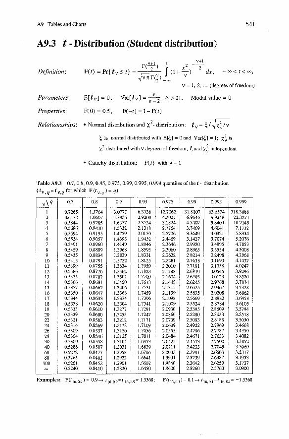
A9 Tables and Charts
A9.3 t - Distribution (Student distribution)
V Parameters: E [ t v ] = 0 , Var [ tv ] = - (V > 2 ) , Modal value = 0 V - 2
Properties: F(0) = 0.5, F(-t) = 1 - F(t)
2 Relationsships: Normal distribution und X - distribution : tv = I&
5 is normal distributed with E[5] = 0 and Var[c] = 1; X; is
distributed with V degrees of freedorn, 5 and independent
Cauchy distribution: F(t) with V = 1
Table A9.3 0.7,0.8,0.9,0.95,0.975,0.99,0.995,0.999 quantiles of the t - distnbution
Examples: F(t16,0,9) = O.9-f t16,0,9=t16,0.9= 1.3368; F(t16,0,1)=0.1-+ 1
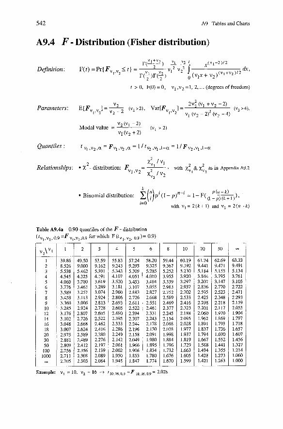
542 A9 Tables and Charts
A9.4 F - Distribution (Fisher distribution)
V l + V 2 V1 r ( 7 ) - - 2
x(V1-2)/2 Definition: F(t) = Pr{ F, 5 t } =
1' 2 "1 dx , r(?)r(+) ( v l x + ~ ~ ) ( ~ 1 + ~ 2 ) ~ ~
t > 0, F(0) = 0 , vl ,v2 =1, 2, . . . (degrees of freedom)
2 "2 2v2 (V1 +V2 - 2)
Parameters: E[FV1,V2] = ~ 2 - 2 (v2 >2), Var[F, , 1 = 0i2 >4), v 1 ( v 2 - 2 ) 2 ( ~ 2 - 4 )
2 Relationships: X - distribution: Fvl ,v2= 7 9 with X; & X; as in Appendix A9.2
Xvz 1 V2 1 2
= 1-F( p(n - k)
BinomiaI distribution: ( l - p ) ( k + l ) ) ' 1=0
w i t h V l = 2 ( k + l ) a n d v 2 = 2 ( n - k )
Table A9.4a 0.90 quantiles of the F - distribution
(tvl,vz,0.9'Fv,,v,,o.9 forwhich F(tv1,v2, 0.9)=0.9)
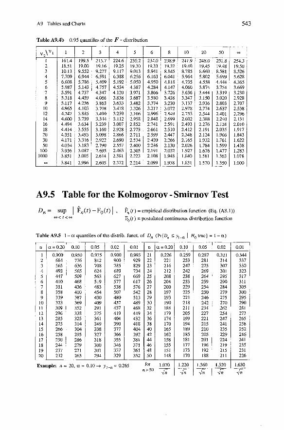
A9 Tables and Charts
Table A9.4b 0.95 quantiles of the F - distribution
Table for the Kolmogorov - Smirnov Test
Dn = SUp I Fn(t) - Fo(t) 1 , F, ( t ) = empirical distribution function (Eq. (A8.l)) - m < t < m F, (t ) = postulated continuous distribution function
Table A9.5 1 - a quantiles of the distrib. funct. of D, ( P ~ { D , < Y,-, I H~ true) = 1 - a )
1.220
J;; 1.630
J;;
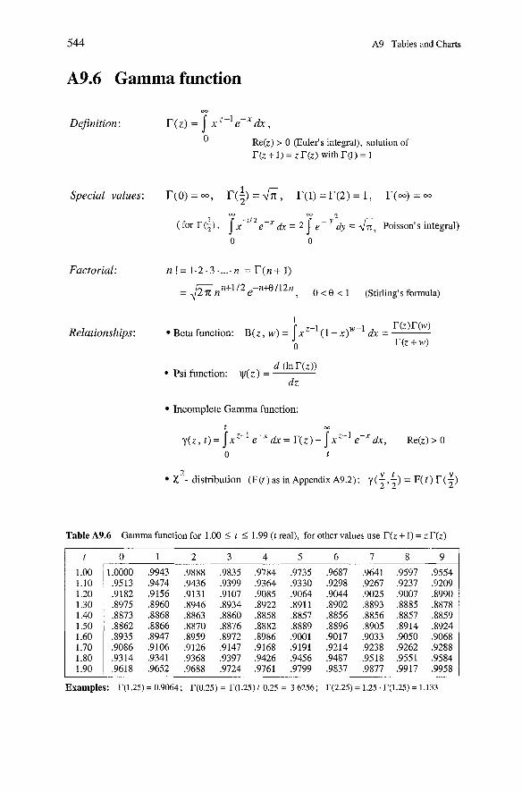
544
A9.6 Gamma function
Definition :
Special values:
Factorial:
Relationships:
A9 Tables and Charts
0 Re(z) > 0 (Euler's integral), solution of T(z + 1) = z T(z) with r(1) = 1
n != 1.2.3 ...: n = r ( n + 1)
= @nn+1/2e-n+B/12n , 0 < 8 < 1 (Stirling's formula)
1 u z ) w
Beta function: B ( z , W ) = Inz- ' (1 - X)"-' dx = --- 0 T(z + W )
Psi function: ~ ( z ) = d (In Uz))
dz
Incomplete Gamma function:
2 X - distribution (F@) as in Appendix A9.2): (f .i) = ~ ( t ) T(;)
Table A9.6 Gamma function for 1.00 5 t 5 1.99 ( t real), for other values use T(z + 1) = z T(z)
t 0 1 2 3 4 5 6 7 8 9
1.00 1.10 1.20 1.30 1.40 1.50 1.60 1.70 1.80 1.90
1.0000 ,9943 ,9888 .9835 ,9784 .9735 ,9687 .9641 .9597 .9554 .9513 .9474 .9436 ,9399 .9364 ,9330 .9298 .9267 ,9237 .9209 .9182 .9156 ,9131 ,9107 .9085 ,9064 ,9044 ,9025 .9007 ,8990 ,8975 ,8960 3946 ,8934 3922 .8911 ,8902 3893 ,8885 3878 ,8873 2868 ,8863 3860 ,8858 ,8857 ,8856 ,8856 ,8857 ,8859 ,8862 ,8866 ,8870 ,8876 .8882 ,8889 ,8896 3905 ,8914 ,8924 ,8935 .8947 ,8959 3972 ,8986 ,9001 ,9017 ,9033 ,9050 .9068 ,9086 ,9106 .9126 ,9147 ,9168 .9191 .9214 ,9238 .9262 .9288 ,9314 ,9341 ,9368 .9397 ,9426 .9456 .9487 .9518 ,9551 .9584 .9618 ,9652 .9688 .9724 ,9761 .9799 .9837 ,9877 .9917 .9958
Examples: r(1.25) = 0.9064; r(0.25) = r(1.25) / 0.25 = 3.6256; r(2.25) = 1.25. r(1.25) = 1.133
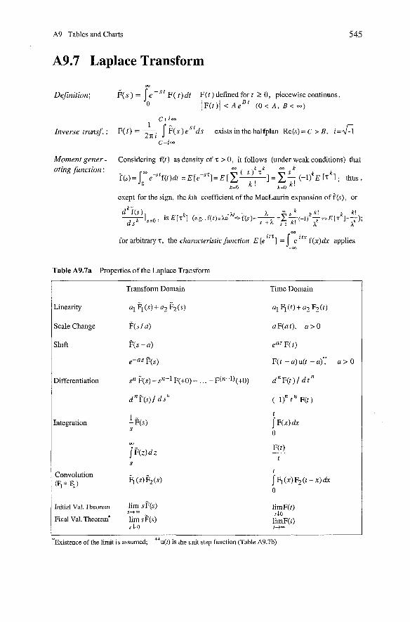
A9 Tables and Charts
A9.7 Laplace Transform
W
Definition: F( s ) = I e - S t F( t ) dt F(t ) defined for t Z 0, piecewise continuos . o I ~ ( t ) l < ~e~~ (0 < A , B < W )
c + i - 1
Inverse irimsf. : F( t ) = - I & s ) es d s exists in the halfplan Re(s) = C > B, i = f i 2n 1
C - i -
Moment gener - Considering f(t) as density of T > 0, it follows (under weak conditions) that ating function: m ( - s f z k k
f(s)= ~ome-s'f(t)d~ = E [ r - " ] = ~ [ x - ] = E I ; thus, k=O k ! k=O k.
exept for the sign, the kth coefficient of the MacLaurin expansion of f (s), or
a itz
for arbitrary T, the characteristic function E [e ] = I e f(x)dx applies -Ce
Table A9.7a Properties of the Laplace Transform
Transform Domain Time Domain
Linearity
Scale Change
Shift
Differentiation
Integration
Convolution (F, * q)
iim s@(s) S+ rn
lim s P(s) s L 0
Initial Val. Theorem
Final Val. ~heorem*
'~xistence of the limit is assumed; **U@) is the unit step function (Table A9.7b)
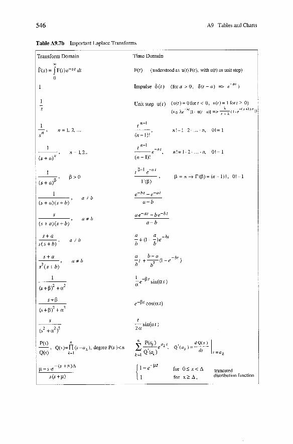
546 A9 Tables and Charts
Table A9.7b Important Laplace Transforms
rransform Domain m
Time Domain
F(t) (understood as u(t) F(t), with u(t) as unit siep)
Impulse 6 (t) (for a > 0 , F(t - a ) => e-sa )
Unit step u( t ) ( ~ ( t ) = 0 for t < 0, ~ ( t ) = 1 fort 2 0) -AI - ( s + A ) a
(e.g. he 11- u( t - U ) ] => ( i -e
a b - a -t + - ( ~ - e - ~ ~ ) b b2
1 -eWpt for 0 2 x < A mncated
for x 2 h , distribution function
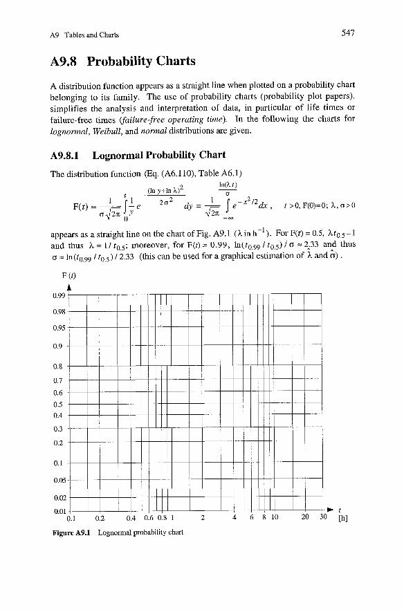
A9 Tables and Charts 547
A9.8 Probability Charts
A distribution function appears as a straight line when plotted on a probability chart belonging to its family. The use of probability charts (probability plot papers). simplifies the analysis and interpretation of data, in particular of life times or failure-free times vailure-free operating time). In the following the charts for lognormal, Weibull, and normal distnbutions are given.
A9.8.1 Lognormal Probability Chart
The distribution function (Eq. (A6.110), Table A6.1) In(h t )
( ~ n y+in h12 - 0
1 ~ ( t ) = - 2 ~ 2 dy = - J e - x 2 ' 2 h , t >o. F(o)=o; A, G > O
0 4G -M
appears as a straight line on the chart of Fig. A9.1 (h in h-' ). For F(t) = 0.5, ht0,5 = 1 and thus h = 1 I t0,5; moreover, for F(t) = 0.99, l ~ ~ ( t ~ , ~ ~ / t0,5) l o = 2,33 and thus o = ln(to.99 1 to,s) 12.33 (this can be used for a graphical estimation of ?L and &) .
Pigure A9.1 Lognormal probability chart
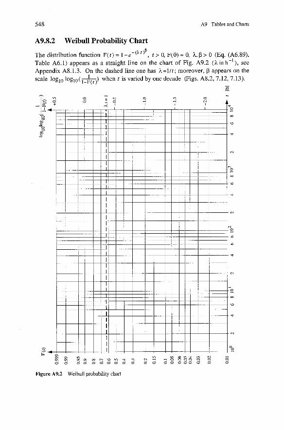
A9 Tables and Charts
A9.8.2 Weibull Probability Chart
The distribution function F( t ) = I - e - @ ' ) ' , t > 0, F(0) = 0, h, ß > 0 (Eq. (A6.89), Table A6.1) appears as a straight line on the chart of Fig. A9.2 (h in h-I), see Appendix A8.1.3. On the dashed line one has h=l / t ; moreover, ß appears on the scale loglo l o g l o ( & - ) ) when t is varied by one decade (Figs. A8.2,7.12,7.13). -
&
m m vI 2 ö 2 2 % 2 ö z g o g g O b b o o ~ o o g 2 Figure A9.2 Weibull probability chart
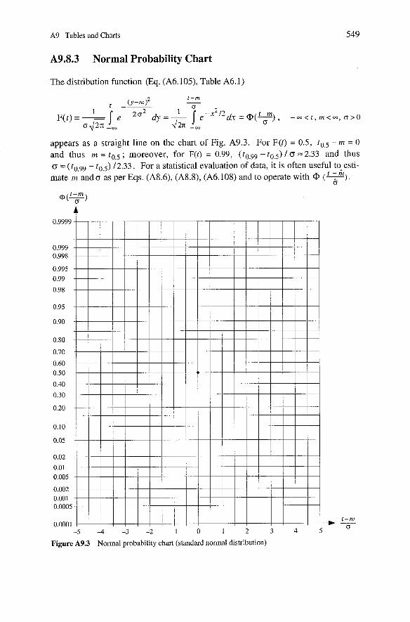
A9 Tables and Charts
A9.8.3 Normal Probability Chart
The distribution function (Eq. (A6.105), Table A6.1)
appears as a straight line on the chart of Fig. A9.3. For F(t) = 0.5, t0.5 - m = 0 and thus m = t0,5 ; moreover, for F ( t ) = 0.99, (t0,99 - t0,5) I G = 2.33 and thus o = (t,„ - to,5) 12.33. For a statistical evaluation of data, it is often useful to-esti- mate m and o as per Eqs. (A8.6), (A8.8), (A6.108) and to operate with @ (e) .
0
Figure A9.3 Normal probability chart (standard normal distribution)

A l 0 Basic Technological Componentis Properties
Table A1O.l gives some basic technological properties of electronic components to Support reliability evaluations.
Table A1O.l Basic technological properties of electronic components
Component
4xed resistors t Carbon film
, Metal film
Wire- wound
Thermistors (PTC, NTC)
Jariable resist.
Cermet Pot., Cermet Trim
Wirewound Pot.
Technology, Characteristics I Sensitive to
A layer of carbon film deposited at high temperature on ceramic rods; +5% usual; medium TC; relatively low dnft (-1 to +4%); failure modes: opens, drift, rarely shorts; elevated noise; 1 G? to 22 MG?; low h (0.2 to 0.4 FIT)
Load, temperature, overvoltage, freq. (> 50MHz), moisture
Evaporated NiCr film deposited on aluminum oxide ceramic; +5% usual; Load, temperature, low TC; low drift (+l%); failure modes: current peaks, drift, opens, rarely shorts; low noise; ESD, moisture 10 Q to 2.4MQ: low h (0.2 FIT)
Usually NiCr wire wound on glass fiber substrate (sometimes ceramic); precision (+0.1%) or power (+5%); low TC; failure modes: opens, rarely shorts between adjacent windings; low noise; O.lG? to 250 k!2 ; medium h (2 to 4 FIT)
Load, temperature, overvoltage, mechanical stress (wire < 25 pm ), moisture
PTC: Ceramic materials ( BaTi03 or SrTiOg with metal salts) sintered at high temperatures, showing strong increase of resistance (103 to 104) within 50°C; medium h (4 to 10 FIT, large values for Current and voltage disk and rod packages) load, moisture NTC: Rods pressed from metal oxides and sintered at hi h temperature, large neg. TC 5 . . (TC - - 1 / T ). failure rate as for PTC
Metallic glazing (often ruthenium oxide) deposited as a thick film on ceramic rods Load, current, and fired at about 800°C; usually 210%; fritting voltage poor linearity (5%); medium TC; failure (< 1.5V), modes: opens, localized wearout, drift; temperature, relatively high noise (increases with age); vibration, 20 C2 - 2 MC2 ; low to medium h (5-20 FIT) CuNi / NiCr wire wound on ceramic rings noise, dust, X cylinders (spindle-operated potentiom.); moisture, normally I 10%; good linearity (1%); frequency (wire) precision or power; low, nonlinear TC; low drift; failure modes: opens, localized wearout, relatively low noise; 10 C2 to 50 kC2: medium to large h (10 to 100 HT)
Application
Low power (51W) moderate tempera- ture (45°C) and frequency (5 50MHz)
Low power ( 5 0.5 W), high accuracy and stability, high freq. ( 5 500 MHz)
High power, high stability, low frequency (5 20 kHz)
PTC: Temperature Sensor, overload protection, etc.
NTC: Compen- sation, control, regulation, stabilization
Should only be 2mployed when there is a need for adjustment during ~peration, fixed resistors have to be preferred for xilibration during testing; load xipability proportional to the part of the resistor med
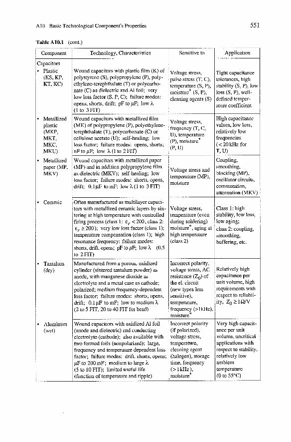
Al0 Basic Technological Component's Properties
Table A1O.l (cont.)
Component
:apacitors Plastic (KS, KP, KT, KC)
Metallized plastic (MKP, MKT, MKC, MKU)
Metallized Paper (MP, MKV)
Ceramic
Tantalum (dry)
Aluminum (wet)
Technology, Characteristics
Wound capacitors with plastic film (K) of polystyrene (S), polypropylene (P), poly- ethylene-terephthalate (T) or polycarbo- nate (C) as dielectric and Al foil; very low loss factor (S, P, C); failure modes: opens, shorts, drift; pF to pR low h (1 to 3FIT)
Wound capacitors with metallized film (MK) of polypropylene (P), polyethylene- terephthalate (T), polycarbonate (C) or cellulose acetate (U); self-healing; low loss factor; failure modes: opens, shorts; nF to p E low h (1 to 2 FIT)
Wound capacitors with metallized paper (MP) and in addition polypropylene film as dielectric (MKV); self-healing; low loss factor; failure modes: shorts, opens, drift; 0.1 pF to mF, low h (1 to 3 FIT)
Often manufactured as multilayer capaci- tors with metallized ceramic layers by sin- tering at high temperature with controlled firing process (class 1: E, < 200, class 2: E, > 200); very low loss factor (class 1); temperature compensation (class 1); high resonance frequency: failure modes: shorts, drift, opens; pF to pF; low h (0.5 to 2 FIT)
Manufactured from a porous, oxidized cylinder (sintered tantalum powder) as anode, with manganese dioxide as electrolyte and a meta1 case as cathode; polarized; medium frequency-dependent loss factor; failure modes: shorts, opens, drift; 0.1 pF to mF; low to medium h (2 to 5 FIT, 20 to 40 FIT for bead)
Wound capacitors with oxidized Al foil (anode and dielectric) and conducting electrolyte (cathode); also available with two formed foils (nonpolarized); large, frequency and temperature dependent loss factor; failure modes: drift, shorts, opens; pF to 200 mF ; medium to large h (5 to 10 FIT); limited useful life (function of temperature and ripple)
Sensitive to
Voltage stress, pulse stress (T, C), temperature (S, P), moisture* (S, P), cleaning agents (S)
Voltage stress, frequency (T, C, U), temperature (P), moisture* (P> U)
Voltage stress and temperature (MP), moisture
Voltage stress, temperature (even during soldering) moisture*, aging at high temperature (class 2)
Incorrect polarity, voltage stress, AC resistance (ZO) of the el. circuit (new types less sensitive), temperature, frequency (>lkHz). moisture*
Incorrect pola& (if polarized), voltage stress, temperature, cleaning agent (halogen), Storage time, frequency (> l r n z ) , moisture*
Application
Tight capacitance tolerances, high stability (S, P), low loss (S, P), well- defined temper- ature coefficient
High capacitance values, low loss, relatively low frequencies (< 20kHz for T, U)
Coupling, smoothing, blocking (MP), oscillator circuits, commutation, attenuation (MKV)
Class 1: high stability, low loss, low aging; class 2: coupling, smoothing, buffering, etc.
Relatively high capacitance per unit volume, high requirements with respect to reliabil- ity, ZO t lS1N
Very high capacit- ance per unit volume, uncritical applications with respect to stability, relatively low ambient temperature (0 to 55OC)

552
Table A1O.l (cont.)
Al0 Basic Technological Component's Properties
Component
Diodes (Si) General purpose
Zener
Transistors Bipolar
FET
I Technology, Characteristics I Sensitive to / Application
PN junction produced from high purity Si by diffusion; diode function based on the recombination of minority carriers in the depletion regions; failure modes: shorts, opens; low h (1 to 3FIT, 0J=400C, 10 FIT for rectifiers with 0 T = 100°C)
Forward current, reverse voltage, temperature, transients, moisture*
I
Heavily doped PN junction (charge carrier I generation in strong electric field and rapid increase of the reverse current at low
Load, temperature, reverse voltages); failure modes: shorts,
moisture* opens, dnft; low to medium h (2 to 4 FIT for voltage regulators ( 8 J = 40°C), 20 to 50 FIT for voltage ref. ( 0 7 = 100°C))
Signal diodes (analog, switch), rectifier, fast switching diodes (Schottky,
Level control, voltage reference (allow for +5% drift)
Swjtch, amplifier, power stage (allow for +20% dnft, +500% for ICBO)
PNP or NPN junctions manufactured using planar technology (diffusion or ion implantation); failure modes: shorts, Opens, thermal fatigue for power transistors; low to medium h (2 to 6 FIT for OJ = 40°C, 20 to 60 FIT for power transistors and 8 = 100°C)
Load, temperature, breakdown voltage (VBCEO, VBEBO), moisture*
Controlled rectifiers (Thyristors, triacs, etc.)
Voltage controlled semiconductor resistance, with control via diode (JFET) or isolated layer (MOSFET); transist. function based on majority carrier transport; N or P channel; depletion or enhancement type (MOSFET); failure modes: shorts, opens, M, medium h (3 to 10 FIT for 8 J = 40°C, 30 to 60 FIT for power transistors and 0 T = 100°C)
Load, temperature, breakdown voltage, ESD, radiation, moisture*
NPNP junctions with lightly doped inner zones (P, N), which can be triggered by a control pulse (thyristor), or a special antiparallel circuit consisting of two thynstors with a single finng circuit (triac); failure modes: drift, shorts, opens; large h (20 to 100 FIT for 0 = 100°C)
Switch (MOS) and amplifier (JFET) for high-resistance circuits (allow for 220% dlift)
Temperature, reverse voltage, nse rate of voltage and current, commutation effects, moisture*
Opto- semiconductors (LED, IRED,
Controlled rectifier, overvoltage and overcurrent protection (allow for 220% drift)
Electrical/optical or opticallelectrical con- verter made with photosensitive semicon- ductor components; transmitter (LED,
photo-sensitive ievices, opto- rouplers, etc.)
IRED, laser diode etc.), receiver (photo- resistor, photo-transistor, solar cells etc.), opto-coupler, displays; failure modes: opens, dnft, short . medi m o large h (2 to 100 FIT, 20.,/no.ofpirel: for LCD); limited useful life
Temperature, cnrrent, ESD, moisture*, mechanical stress
Displays, Sensors, galvanic sepa- ration, noise rejection (allow for 230% drift)
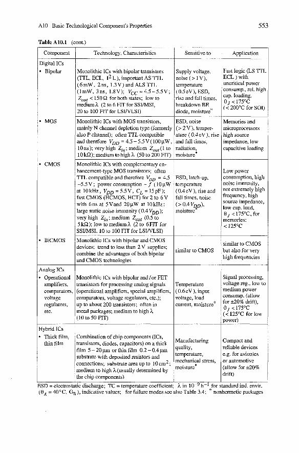
Al0 Basic Technological Component's Properties 553
Table A1O.l (cont.)
Component
Digital ICs Bipolar
MOS
CMOS
BiCMOS
Analog ICs
Operational amplifiers, comparators, voltage regulators, etc.
Hybrid ICs Thick film, thin film
Application Technology, Charactenstics
Monolithic ICs with bipolar transistors (TTL, ECL, L), important AS TTL (6mW, 2ns, 1.3V) and ALS TTL (ImW, 3ns, 1.8V); VCC = 4.5-5.5V; Zout < 150 B for both states; low to medium h (2 to 6 FIT for SSI/MSI, 20 to 100 FIT for LSUVLSI)
Fast logic (LS TTI ECL ) with uncntical power consump., rel. higl cap. loading, 8 j < 175°C (< 200°C for SOI:
Sensitive to
Supply voltage, noise (> lV) , temperature (OSeV), ESD, rise and fall times, breakdown BE diode, moisture*
Memones and microprocessors high source impedance, low capacitive loading
Monolithic ICs with MOS transistors, mainly N channel depletion type (formerly also P channel); often TTL compatible and therefore VDD = 4.5 - 5.5 V ( 100 pW , 10 ns ); very high Zi, ; medium Zout (1 to 10 kQ); medium to high h (50 to 200 FIT)
Monolithic ICs with complementary en- hancement-type MOS transistors; often TTL compatible and therefore VDD = 4.5 -5.5V ; power consumption - f ( 10 pW at10kHz,VDD=5.5V,CL=15pF); Cast CMOS (HCMOS, HCT) for 2 to 6 V with 6 ns at 5 Vand 20 pW at 10 kHz : large static noise immunity (0.4 VDD); very high Zi, ; medium Zmt (0.5 to 5 kB); low to medinm h (2 to 6FIT for SSI/MSI, 10 to 100 FIT for LSINLSI)
Low power consumption, high noise immunity, not extremely higi- frequency, high source impedance, low cap. load, 8 j < 175OC, f0r memones: 1125°C
ESD, noise (> 2 V ), temper- ature ( 0.4eV), rise and fall times, radiation, moisture*
ESD, latch-up, temperature (0.4eV),riseand fall times, noise (> 0.4 VDD), moisture*
Monolithic ICs with bipolar and CMOS devices; trend to less than 2 V supplies; rombine the advantages of both bipolar and CMOS technologies
Combination of chip components (ICs, transistors, diodes, capacitors) on a thick tilm 5 - 20 pm or thin film 0.2 - 0.4 pm Substrate with deposited resistors and :onnections; substrate area up to 10 cm2 ; medium to high h (usually detennined by the chip components)
similar to CMOS similar to CMOS but also for very
high frequencies
Monolithic ICs with bipolar and /or FET transistors for processing analog signals (operational amplifiers, special amplifiers, iomparators, voltage regulators, etc.); up to about 200 transistors; often in meta1 packages; medium to high h J0 to 50 FiT)
Manufacturing Compact and quality, reliable devices temperature, e.g. for avionics mechanical stress, or automotive moisture* (ailow for +20%
drift)
Signal processing, Temperature voltage reg., low tc (0.6eV ), input medium Power voltage, load cOnSUmp CU,.rent, moisture* for dnft),
8 j < 175°C (< 125°C for low power)
I (BA = 40°C, GB ), indicat&e values; foi failure modes See also Table 3.4; * nonhermetic packages
I
!SD = electrostatic discharge; TC = temperature coefficient; h in 1 0 - ~ h-I for standard ind. envir.
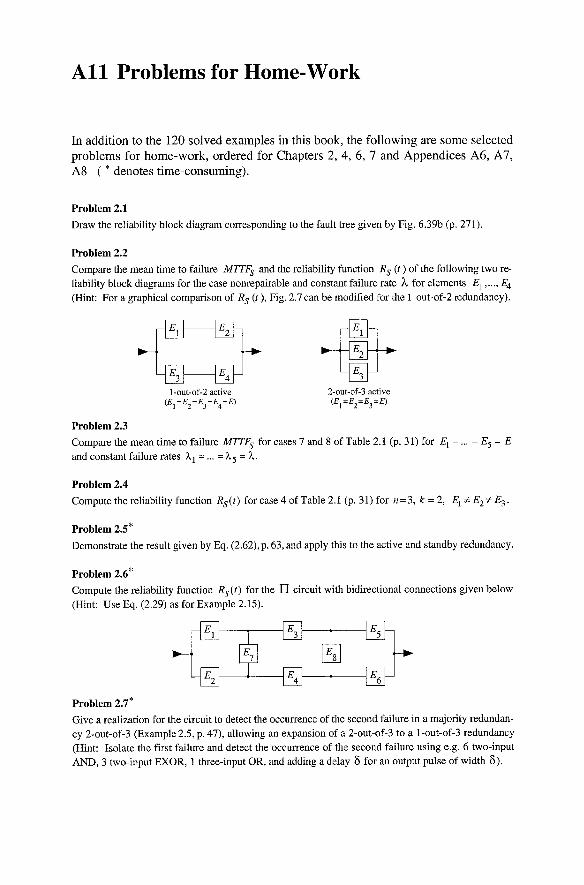
A l l Problems for Horne-Work
In addition to the 120 solved examples in this book, the following are some selected problems for home-work, ordered for Chapters 2, 4, 6, 7 and Appendices A6, A7, A8 ( * denotes time-consuming).
Problem 2.1 Draw the reliability block diagram corresponding to the fault tree given by Fig. 6.39b (p. 271).
Problem 2.2 Compare the mean time to failure M T and the reliability function Rs (t ) of the following two re- liability block diagrams for the case nonrepairable and constant failure rate for elements E, ,..., E4 (Hint: For a graphical comparison of Rs (t ), Fig. 2.7 can be modified for the 1-out-of-2 redundancy).
y& E4 +E& 1-out-of-2 active 2-out-of-3 active
(E = E = E = E =E) 1 2 3 4
( E =E = E =E) 1 2 3
Problem 2.3
Compare the mean time to failure M T for cases 7 and 8 of Table 2.1 (p. 31) for E, = ... = E5 = E and constant failure rates hl = ... = h5 = h .
Problem 2.4 Compute the reliability function Rs(t) for case 4 of Table 2.1 (p. 3 1) for n= 3, k = 2, EI + E2 + E3.
Problem 2.5*
Demonstrate the result given by Eq. (2.62), p. 63, and apply this to the active and standby redundancy.
Problem 2.6* Compute the reliability function Rs(t) for the n circuit with bidirectional connections given below (Hint: Use Eq. (2.29) as for Example 2.15).
Problem 2.7* Give a realization for the circuit to detect the occurrence of the second failure in a majority redundan- cy 2-out-of-3 (Example 2.5, p. 47), allowing an expansion of a 2-out-of-3 to a 1-out-of-3 redundancy (Hint: Isolate the first failure and detect the occurrence of the second failure using e.g. 6 two-input AND, 3 two-input EXOR, 1 three-input OR, and adding a delay 6 for an output pulse of width 6).
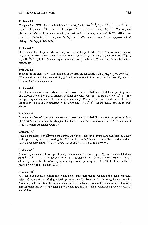
A l l Problems for Home-Work
Problem 4.1
Compute the M T R s for case 5 of Table 2.1 (p. 31) for hl = 10-~ h-l, h2 = 1 0 - ~ h-', h3 = 10-2 h-', h, = W3 h-', h, = 1 0 - ~ h-', h6 = 10" h-l, h, = I O - ~ h-', and p = ... = = 0.5 h" . Compare the obtained M V R s with the mean repair (restoration) duration at system level MDTs (Hint: use results of Table 6.10 to compute MTTFso and P A S , and assume (as an approximation) MUTs = MTTFso in Eq. (6.291)).
Problem 4.2 Give the number of spare parts necessary to cover with a probability y 2 0.9 an operating time of 50,000h for the system given by case 6 of Table 2.1 (p. 31) for hl = & = 4 = 10-~h-', h, = 10"h-' (Hint: Assume equal allocation of y between E, and the 2-out-of-3 active redundancy).
Problem 4.3 Same as for Problem 4.2 by assuming that spare parts are repairable with pi=pz =p3 =pv= 0.5 h-l (Hint: consider only the case with Rs (t ) and assume equal allocation of y between E, and the 2-out-of-3 active redundancy).
Problem 4.4 Give the number of spare parts necessary to cover with a probability y 2 0.9 an operating time of 50,000h for a 1-out-of-2 standby redundancy with constant failure rate h = 10-~ h-' for the operating element (?L= 0 for the reserve element). Compare the results with those obtained for an active 1-out-of-2 redundancy with failure rate h = 10-~ h-l for the active and the reserve element.
Problem 4.5 Give the number of spare parts necessary to cover with a probability y 2 0.9 an operating time of 50, OOOh for an item with Erlangian distributed failure-free times with h = 10-~ h-' and n = 3 (Hint: Consider Appendix A6.10.3).
Problem 4.6* Develop the expression allowing the computation of the number of spare parts necessary to cover with a probability 2 y an operating time T for an item with failure-free times distributed according to a Gamma distribution (Hint: Consider Appendix A6.10.3, and Table A9.7b).
Problem 4.7* A series-system consists of operationally independent elements 4 ,..., E, with constant failure rates Al ,...,?L, . Let c, be the cost for a repair of element Ei. Give the mean (expected value) of the repair cost for the whole system during a total operating time T (Hint: Use results of Section 2.2.6.1 and Appendix A7.2.5).
Problem 4.8* A system has a constant failure rate A and a constant repair rate p. Compute the mean (expected value) of the repair cost during a total operating time T. given the fixed cost co for each repair. Assuming that down time for repair has a cost cd per hour, compute the mean value of the total cost for repair and down time during a total operating time T, (Hint: Consider Appendices A7.2.5 and A7.8.4).
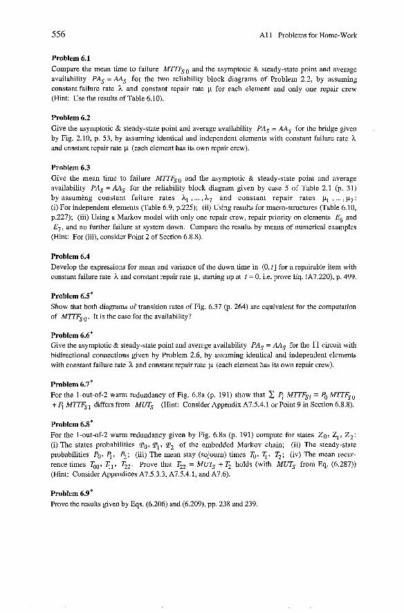
A l 1 Problems for Home-Work
Problem 6.1 Compare the mean time to failure MITFso and the asymptotic & steady-state point and average availability PAS =AAS for the two reliability block diagrams of Problem 2.2, by assuming constant failure rate h and constant repair rate p for each element and only one repair Crew (Hint: Use the results of Table 6.10).
Problem 6.2 Give the asymptotic & steady-state point and average availability PAs = AAS for the bridge giveu by Fig. 2.10, p. 53, by assuming identical and independent elements with constant failure rate h and constant repair rate p (each element has its own repair crew).
Problem 6.3 Give the mean time to failure M7TFs0 and the asymptotic & steady-state point and average availability PAs = AAS for the reliability block diagram given by case 5 of Table 2.1 (p. 31) by assuming constant failure rates hl , ... , h7 and constant repair rates pl , ... ,P,: (i) For independent elements (Table 6.9, p.225); (ii) Using results for macro-stmctures (Table 6.10, p.227); (iii) Using a Markov model with only one repair crew, repair priority on elements E6 and E7, and no further failure at system down. Compare the results by means of numerical examples
(Hint: For (iii), consider Point 2 of Section 6.8.8).
Problem 6.4 Develop the expressions for mean and variance of the down time in (0, t ] for a repairable item with constant failure rate h and constant repair rate p, starting up at t = 0, i.e. prove Eq. (A7.220), p. 499.
Problem 6.5* Show that both diagrams of transition rates of Fig. 6.37 (p. 264) are equivalent for the computation of MTT4 o. It is the case for the availability?
Problem 6.6* Give the asymptotic & steady-state point and average availability PAs = AAS for the n circuit with bidirectional connections given by Problem 2.6, by assuming identical and independent elements with constant failure rate h and constant repair rate p (each element has its own repair crew).
Problem 6.7* For the 1-out-of-2 warm redundancy of Fig. 6.8a (p. 191) show that 2 MTTFSi = Po M q o + 4 M q l differs from MUTs (Hint: Consider Appendix A7.5.4.1 or Point 9 in Section 6.8.8).
Problem 6.8* For the 1-out-of-2 warm redundancy given by Fig. 6.8a (p. 191) compute for states Z o , q, Z 2 : (i) The states probabilities PO, P I , P2 of the embedded Markov chain; (ii) The steady-state probabilities Po, 4 , P2 ; (iii) The mean stay (sojourn) times q, q , T2 ; (iv) The mean recur- rence times Tao, q,, T22. Prove that T22 = MUTS + T2 holds (with MUTs from Eq. (6.287)) (Hint: Consider Appendices A7.5.3.3, A7.5.4.1, and A7.6).
Problem 6.9* Prove the results given by Eqs. (6.206) and (6.209), pp. 238 and 239.
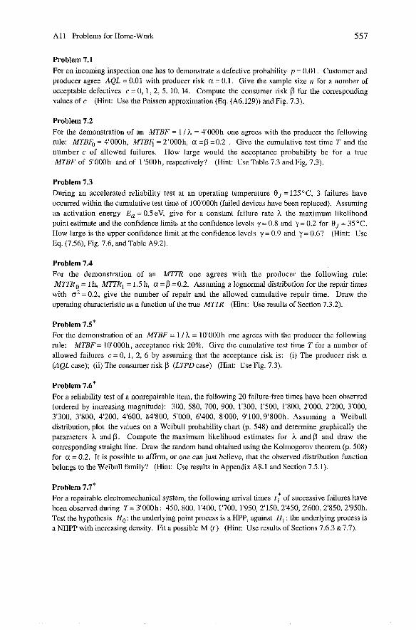
A l 1 Problems for Home-Work
Problem 7.1 For an incoming inspection one has to demonstrate a defective probability p = 0.01. Customer and producer agree AQL = 0.01 with producer risk a = 0.1. Give the sample size n for a number of acceptable defectives c = 0, 1,2, 5, 10, 14. Compute the consumer risk ß for the corresponding values of c (Hint: Use the Poisson approximation (Eq. (A6.129)) and Fig. 7.3).
Problem 7.2 For the demonstration of an MTBF = I / h = 4'000h one agrees with the producer the following rule: MTB6 = 4'000h, MTB3 = 2'000h, a =ß =0.2 . Give the cumulative test time T and the number c of allowed failures. How large would the acceptance probability be for a true MTBF of 5'000h and of 1 '500h, respectively? (Hint: Use Table 7.3 and Fig. 7.3).
Problem 7.3 During an accelerated reliability test at an operating temperature BJ =125"C, 3 failures have occurred within the cumulative test time of 100'000h (failed devices have been replaced). Assuming an activation energy E, = 0.5eV, give for a constant failure rate h the maximum likelihood point estimate and the confidence limits at the confidence levels y= 0.8 and y= 0.2 for BJ = 35'C. How large is the upper confidence limit at the confidence levels y = 0.9 and y = 0.6? (Hint: Use Eq. (7.56), Fig. 7.6, and Table A9.2).
Problem 7.4 For the demonstration of an M7TR one agrees with the producer the following rule: MTTRo = 1 h, MTTRl = 1.5 h, a =ß =0.2. Assuming a lognormal distnbution for the repair times
with o2 = 0.2, give the number of repair and the allowed cumulative repair time. Draw the operating characteristic as a function of the true MTTR (Hint: Use results of Section 7.3.2).
Problem 7.5* For the demonstration of an MTBF = 1 / h = 10'000h one agrees with the producer the following rule: MTBF = 10'000h, acceptance risk 20%. Give the cumulative test time T for a number of allowed failures c = 0, 1, 2, 6 by assuming that the acceptance risk is: (i) The producer nsk a (AQL case); (ii) The consumer risk ß (LTPD case) (Hint: Use Fig. 7.3).
Problem 7.6* For a reliability test of a nonrepairable item, the following 20 failure-free times have been observed (ordered by increasing magnitude): 300, 580, 700, 900, 1'300, 1'500, 1'800, 2'000, 2'200, 3'000, 3'300, 3'800, 4'200, 4'600, ä4'800, 5'000, 6'400, 8'000, 9'100,9'800h. Assuming a Weibull distribution, plot the values on a Weibull probability chart (p. 548) and determine graphically the Parameters h and ß. Compute the maximum likelihood estimates for h and ß and draw the corresponding straight line. Draw the random band obtained using the Kolmogorov theorem (p. 508) for a = 0.2. It is possible to affirm, or one can just believe, that the observed distribution function belongs to the Weibull family? (Hint: Use results in Appendix A8.1 and Section 7.5.1).
Problem 7.7* For a repairable electromechanical System, the following amval times t * of successive failures have been observed during T = 3'000h: 450, 800, 1'400, 1'700, 1'950, 2'150, 2'450, 2'600, 2'850, 2'950h. Test the hypothesis H,,: the underlying point process is a HPP, against H1 : the underlying process is a NHPP with increasing density. Fit a possible M (t ) (Hint: Use results of Sections 7.6.3 gr7.7).
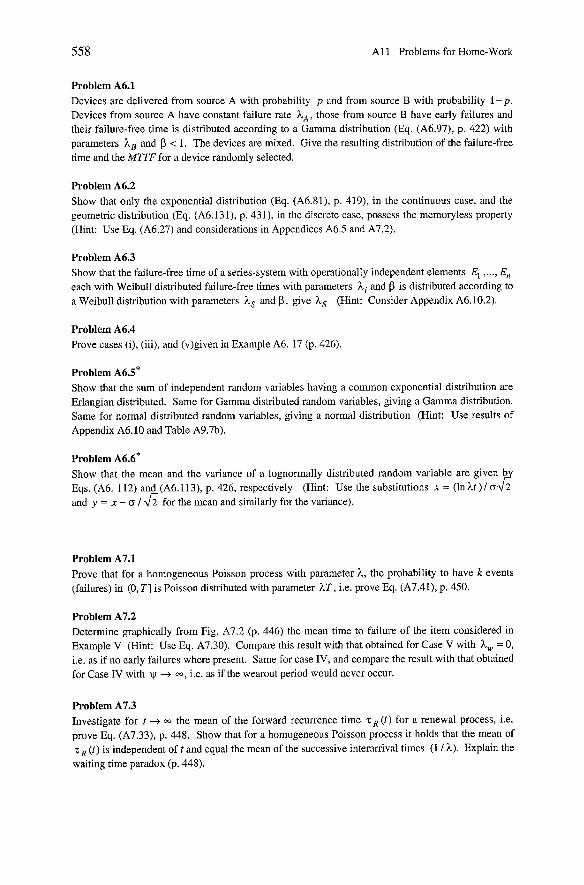
A l 1 Problems for Home-Work
Problem A6.1 Devices are delivered from source A with probability p and from source B with probability I - p. Devices from source A have constant failure rate LA, those from source B have early failures and their failure-free time is distributed according to a Gamma distribution (Eq. (A6.97), p. 422) with parameters hB and ß < 1. The devices are mixed. Give the resulting distnbution of the failure-free time and the M7TF for a device randomly selected.
Problem A6.2 Show that only the exponential distribution (Eq. (A6.81), p. 419), in the continuous case, and the geometnc distribution (Eq. (A6.131), p. 431), in the discrete case, possess the memoryless property (Hint: Use Eq. (A6.27) and considerations in Appendices A6.5 and A7.2).
Problem A6.3 Show that the failure-free time of a series-system with operationally independent elements E, ,..., E, each with Weibull distributed failure-free times with parameters h i and ß is distributed according to a Weibull distnbution with parameters hs and ß, give hs (Hint: Consider Appendix A6.10.2).
Problem A6.4 Prove cases (i), (iii), and (v)given in Example A6. 17 (p. 426).
Problem A ~ S * Show that the sum of independent random variables having a common exponential distribution are Erlangian distributed. Same for Gamma distnbuted random variables, giving a Gamma distribution. Same for normal distributed random variables, giving a normal distribution (Hint: Use results of Appendix A6.10 and Table A9.7b).
Problem ~ 6 . 6 * Show that the mean and the variance of a lognormally distnbuted random variable Eqs. (A6. 112) and (A6.113), p. 426, respectively (Hint: Use the substitutions X = and y = X - o I & for the mean and similarly for the variance).
Problem A7.1 Prove that for a homogeneous Poisson process with parameter h, the probability to have k events (failures) in (0, T] is Poisson distributed with parameter AT, i.e. prove Eq. (A7.41), p. 450.
Problem A7.2 Determine graphically from Fig. A7.2 (p. 446) the mean time to failure of the item considered in Example V (Hint: Use Eq. A7.30). Compare this result with that obtained for Case V with h, = 0, i.e. as if no early failures where present. Same for case IV, and compare the result with that obtained for Case IV with -t W, i.e. as if the wearout penod would never occur.
Problem A7.3 Investigate for t + m the mean of the fonvard recurrence time z R ( t ) for a renewal process, i.e. prove Eq. (A7.33), p. 448. Show that for a homogeneous Poisson process it holds that the mean of
( t ) is independent o f t and equal the mean of the successive interarrival times (1 I L). Explain the waiting time paradox (p. 448).
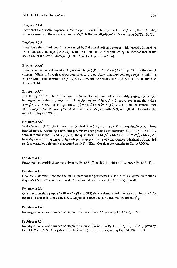
Al 1 Problems for Home-Work
Problem A7.4 Prove that for a nonhomogeneous Poisson process with intensity m(t ) = dM(t ) 1 dt , the probability to have k events (failures) in the interval (0, T] is Poisson distributed with parameter M(T) - M(0).
Problem A7.5 Investigate the cumulative damage caused by Poisson distributed shocks with intensity h, each of which causes a damage 5 > 0 exponentially distnbuted with parameter q > 0, independent of the shock and of the present damage (Hint: Consider Appendix A7.8.4).
Problem ~ 7 . 6 * Investigate the renewal densities hird(t) and hdu (t ) (Eqs. (A7.52) & (A7.53), p. 454) for the case of constant failure and repair (restoration) rates h and p. Show that they converge exponentially for t + W with a time constant 1 I (h + p) -; 1 I p toward their final value h p 1 (h + p) = h (Hint: Use Table A9.7b).
Problem ~ 7 . 7 * Let O<T;<T;< ... be the occurrence times (failure times of a repairable system) of a non- homogeneous Poisson process with intensity m(t ) = dM(t ) I dt > 0 (measured from the origin t = T 0 = 0 ). Show that the quantities = M (T;) < = M (T 2) < ... are the occurrence times in a homogeneous Poisson process with intensity one, i.e with M(t)= t (Hint: Consider the remarks to Eq. (A7.200)).
Problem ~ 7 . 8 * In the interval (0, T], the failure times (arrivai times) T;< ... <T,*< T of a repairable system have been observed. Assuming a nonhomogeneous Poisson process with intensity m(t ) = &I (t ) 1 dt > 0, show that (for given T and v(T)= n), the quantities 0 < M (T;) 1 M(T) < ... < M (T: ) 1 M(T) I 1 have the same distribution as if they where the order statistics of n independent identically distributed random variables uniformly distributed on (0,l) (Hint: Consider the remarks to Eq. (A7.206)).
Problem A8.1 Prove that the empirical variance given by Eq. (A8.10), p. 507, is unbiased (i.e. prove Eq. (A8.11)).
Problem A8.2 Give the maximnm likelihood point estimate for the Parameters A and ß of a Gamma distnbution (Eq. (A6.97), p. 422) and for m and o of a normal distribution (Eq. (A6.105), p. 424).
Problem A8.3 Give the procedure (Eqs. (A8.91) - (A8.93), p. 532) for the demonstration of an availability PA for the case of constant failure rate and Erlangian distributed repair times with parameter PP.
Problem ~ 8 . 4 *
Investigate mean and variance of the point estimate h = k I T given by Eq. (7.28), p. 296.
Problem A M * Investigate mean and variance of the poin; estimate h = (k - 1)1 (tl + . . . + tk + (n - k) t k ) given by Eq. (A8.35), p. 5 15. Apply this result to h = n 1 (tl + . . . + t, ) given by Eq. (A8.28), p. 5 13.

Acronyms
ACM AFCIQ ANS1 AQAP ASQC BWB CECC CENELEC CNET
DGQ DIN DOD EOQC EOSESD ESA ESREF ETH EXACT GIDEP GPO GRD IEC (CEI) IECEE IECQ IEEE IES IPC IRPS ISO MIL-STD NASA NTIS RAMS RIAC Rel. Lab. RL
SAQ SEV SNV SOLE VDWDE
: Association for Computing Machinery, New York, NY 10036 : Association Francaise pour le Controle Industrie1 de la Qualitk, F-92080 Paris : Amencan National Standards Institute, New York, NY 10036 : Allied Quality Assurance Publications (NATO-Countries) : American Society for Quality Control, Milwaukee, W1 53203 : Bundesamt für Wehrtechnik und Beschaffung, D-56000 Koblenz : Cenelec Electronic Components Committee, B-1050 Bruxelles : European Committee for Electrotechnical Standardization, B-1050 Bruxelles : Centre National d'Etudes des Telecommunications, F-22301 Lannion : Deutsche Gesellschaft fur Qualität, D-60549 Frankfurt a. M. : Deutsches Institut für Normung, D-14129 Berlin 30 : Departement of Defense, Washington, D.C. 20301 : European Organization for Quality Control, B-1000 Brussel : Electrical OverstressElectrostatic Discharge : European Space Agency, NL-2200 AG Noordwijk : European Symp. on Rel. of Electron. Devices, Failure Physics and Analysis : Swiss Federal Institute of Technology, CH-8092 Zürich : Int. Exchange of Authentic. Electronic Comp. Perf. Test Data, London, NW4 4AP : Government-Industry Data Exchange Program, Corona, CA 91720 : Govemment Printing Office, Washington, D.C. 20402 : Gruppe Rüstung, CH-3000 Bem 25 : International Electrotechnical Commission, CH-1211 Genkve 20, P.O.Boxl3 1 : IEC System for Conformity Testing and Certif. of Electrical Equip., CH-121 lGent5ve20 : IEC Quality Assessment System for Electronic Components, CH-1211 Genkve 20 : Institute of Electrical and Electronics Engineers, Piscataway, NJ 08855-0459 : Institute of Environmental Sciences, Mount Prospect, IL 60056 : Institute for Interconnecting and Packaging EI. Circuits, Lincolnwood, IL 60646 : International Reliability Physics Symposium (IEEE), USA : International Organisation for Standardization, CH-1211 Genkve 20, P.O.Box56 : Military (USA) Standard, Standardiz. Doc. Order Desk, Philadelphia, PA191 11-5094 : National Aeronautics and Space Administration, Washington, D.C. 20546 : National Technical Information Service, Springfield, VA 22161-2171 : Reliability, Availability, Maintainability, Safety; also Rel. & Maint. Symposium, IEEE : Reliability Information Analysis Center, Utica, NY 13502-1348 (formerly RAC) : Reliability Laboratory at the ETH (since 1999 at EMPA S173, CH-8600 Dübendorf) : Rome Laboratory, Griffiss M B , NY 13441-4505 : Schweizerische Arbeitsgemeinschaft für Qualitätsfördernng, CH-4600 Olten : Schweizerischer Elektrotechnischer Verein, CH-8320 Fehraltorf : Schweizerische Normen-Vereinigung, CH-8008 Zürich : Society of Logistic Engineers, Huntsville, AL 35806 : Verein Deutscher 1ng.Nerband Deut. Elektrotechniker, D-60549 Frankfurt a. M.
Index
(less relevant places (not bold) are omitted by some terms)
A pnon / a posteriori probability 401,511 Absolutely continuous 403 Absorbing state 471-72 Accelerated test 35,81,86,98,99,102,307-12,
352,426,535 (see also 312-34) Acceleration factor 37,99,308-11 Acceptable Quality Level (AQL) 86,284-86,530 Acceptance line 283-84,301-02,528-29 Acceptance test -+ Demonstration Accessibility 8,118,151-52 Accident prevention 9,362 Accumulated -+ Cumulative Acquisition cost 11,13,14,357 Activation energy 37,97,99,103,308-09, Active redundancy 43,44,61-64,195,206,210,
211,225,227,361 Addition theorem 397,399 Adjustment 118,152 Age replacement 134,234 Aging 6,405 (see also Wearout and Bad-as-old) Alarm circuit 47 Allocation (reliability) 67 Alternating renewal process 168,452-56 Alternative hypothesis 280,291,298,305,525-26 Alternative investigation methods 267-76 AMSAA model 330 Anderson -Darling statistic 534 Antistatic container 148 AOQ l AOQL 281-82 Aperture in shielded enclosure 144 Approximate expressions 59,61,131-34,179-
8O,l88,192,195,198-2OO, 206,211,227, 219-30,236,238,240,243,245,266,430
Approximation of a reliability function 192 Approximation of a repair funct. 114-15,198-200 AQL + Acceptable Quality Level Arbitrary failure and repair rates 164,168,186,
200,23 1-32 Arbitra~y initial conditions (one item) 176-78 Arbitrary repair rate 177,185,188,200,206,
215,241,489,490 Arithmetic random variable 402,428-31 Arrhenius model 37,97,102,307-09 Arrival rate 494,501
Arrival time 321,331,442,494,496 As-bad-as-old 40,497 As-good-as-new 5,6,8,9,40,164,171,232,
234,236,242,249,251,253,254,365,294, 319,353,356,358,359,404,497
Assessed reliability 3 Asymptotic behavior 178-80,447-50,455,474-76,
486-88,491-92 (see also Stationary and Steady-state)
Asynchronous logic 149 Automatic test equipment (ATE) 88 Availability
demonstration 291-92,293,531-32 estimation 289-90,293,523-24
Average availability (AA) 9,171-72,176,177, 476,487 (see also Intrinsic, Operational, Overall, Point, Technical availability)
Average Outgoing QuaIity (AOQ) 281-82 Axioms of probability theory 394
Backdriving 340 Backward recurrence time 447 Bad-as-old (BAO) 40,405,497 Bathtub curve 6-7,422 Bayes theorem 401,414 Bayesian estimate / statistics 414,511 Bernoulli distnbution -t Binomial distribution Bernoulli trials 427-28,431,433,513 Bernoulli variable 427 Bidirectional connection 31,53,554 Binary decision diagram (BDD) 271 Binomial distribution 408-09,427-29,517-20,
527-28 Birth and death process 131,207,211,479-83 BIST -+ Built-in self-test BIT + Built-in test BITE + Built-in test equipment Black model 97 Bonding 95,100 Boolean function method 58-61 Bottom-up 72, 156,158,355 Boundary-scan 149 Bounds 59,179-80 Branching process 499
Index
Breakdown 96-97,102,106,140,144,145 Bridge structure 31,5344 Built-in self-test (BIST) 150 Built-in test 66,116-1 18,149-51 Built-in test equipment (BITE) 116 Burn-in 6,339,342,352
capability 13,66,72,154,248,352,376,479 Capacitors 140,141,143,146,521 Captured 181 CASE 157 Cataleptic failure 4,6 Causes for defects 66,155-57,329,341 Causes for failures 3-4 Cause-to-effects-analysis 15,66,72-80,153,
15748,329,356 Cause-to-effects-chart 76,356 CDM -+ Charged device model Censoring 295,296,298,323,324,331,504,s 15 Central limit theorem 126,434-37,449 Centralized logistic Support 125-29,130 Ceramic capacitor 140,143,146,147,521 Change 379 Chapman-Kolmogorov equations 462 Charactenstic function 539,545 Characterization 90-92,108 Charge spreading 103 Charged device model 94 Chebyshev inequality 411,293,433,434 Check list 79,120,372-75,376-82,383-87 Chi-square ( x 2 ) distribution 408-09,423,540 Chi-square ( x 2 ) test 3 16- 18,535-38 Classical probability 395 Clock 66,144,146,150,151 Clustering of states 222 CMOS tenninals 145 Coating 142 Coefficient of variation 128,411 Coffin-Manson 109,3 11 Coherent System 57,61 Cold redundancy -+ Standby redundancy Common-cause 72,260-64 Common-mode currents 144 Cornmon mode failures 42,66,72,260,361 Comparative studies 15,25,26,31,44,48-49,78,
103,116,119,130,133,164,194,220-21,234, 261,446,550-54
Complement (complementary events) 392 Complex structure 52,231 Complex ystern 64-66 Composite shmoo-plots 91 Compound failure rate 3 10 Compound process + Cumulative process
Computer-aided reliability prediction 272-76 Concurrent engineenng 1,11,16,17,19,21,
353,357,360,376 Conditional density Idistribution function
404,412-14,485,491,495,497 Conditional expected value 405,414 Conditional failure rate 405,497 Conditional probability 396-97,444,460,494,501 Confidence ellipse 278-79,518-19 Confidence interval 279,290,297,516-24 Confidence level 516 Confidence limits 516
availability 289-90,523-24 failure rate h 296-97,520-23 f ah re rate hs at system level 298 Parameters lognormal distribution 305 unknown probability 278-80,5 16-520
Configuration accounting 379 Configuration auditing 374,378-79 Configuration control 158,374,379 Configuration management 16,21,152,157,
158,335,353,378-81 Conformal coating -+ Coating Congruential relation 274 Connector 140,145,146,148,152 Consecutive k-out-of-n system 45 Consistent estimates 5 11-12 Constant acceleration test 339 Constant failure rate 6-7,35,40,172,165,177,
179-80,294-303,405,419-20,450-51,460-83 Constant repair rate 171,181,177,182-84,189-
96,207-1 1,213-30,238-40,243-71,46043 Consumer risk 86,281,284,291,299,302,
526,532 Contamination 85,93,98 Continuity test 88 Continuous random variable 403-04,408,412-14 ControIlability 149 Convergence almost sure T, Conv. with prob. one Convergence in probability 433 Convergence quickness 127,179-80,279,290,
297,303,313,394,506,507-08,519,522,530 Convergence with probability one 434 Convolution 416-17,545 Cooling 84,140-42,146 Corrective actions 16,21,22,72,73,77,80,104-
05,153,336,389-90 Corrective maintenance 8,113,118,120,154,353 Correlation 78,415,425,440-41 Corrosion 83,85,98-99,102,103,142,311 Cost I cost equation 12,14,136-38,235,242-43,
342-49,357,364,369-70,372,376,428,476 Cost effectiveness 13,353
Cost optimization 11,13,16,353,357 Count function 442,451,493,499 Covariance matrix 4 15 Coverage -+ Incomplete coverage, Test Cover. Cracks 85,93,102,104,106,108,109,111 Cramer - von Mises test 322,534 Critical design review -+ Design review Critical operating states 264 Criticality 72-73,78,153,158,161 Criticality grid 1 criticality matrix 72-73 Cumulated states 259,477 Cumulative damage 499,559 Cumulative operating time 294-303,309,515 Cumulative process 237-38,498-500 Customer requirements 365-68,369-7 1 Cut Sets -+ Minimal cut sets Cut sets theorem 509,512 Cutting of states 222,230,273 Cycle 275,455-57,491
Damage 85,93,94,95,100,104,106,107,109, 110,311,312,329,336,337,340
Damp test -T) Humidity test Data collection 21,22,23,360-61,388-90 Data retention 89,97-98 DC Parameter 88,92 De Moivre-Laplace theorem 434,518 Death process 61-63 Debug test 159 Debugging 153,158 Decentralized logistic Support 129-30,134 Decoupling capacitor 66,143,146 Defect 354
152-61,302-04,341,343,344-49,362 localization 337 prevention 66,78,155-59
(see also Dynamic defect) Defect tolerant 152-53,155 Defective prob. 12,86,277-86,337,341,343 Deferred cost 12,14,342,342,344-47 Definition of probability 394-95 Deformation mechanisms I energy 109,3 41 Degradation 4,7,66,92,96,101,112,248,264 Degree of freedom 423,540-42 Demonstration
availability 291-92,293,531-32 defective (or unknown) probability p 283, 280-86,287-88,526-30 . const. failure rate h or MTBF=l I h 301, 298-303,370-71 M7TR 305-07,371
Dendrites 95,100
Density 403,408,413 Dependability 9,11,13,19,354,366,367,479 Derating 33,82,84,86,139-40,354 Design FMEAIEMECA 72,78 Design guidelines 25-27,66,77,80,84,374,377
maintainability 149-52 reliability 139-48 software quality 152-61
Design reviews 21,27,77,79,107,120,153,159, 354,374,378,381,383-87
Design d e s + Rules Destructive analysis 104 Device under test (DUT) 88 Diagnosis -+ Fault isolation Diagram of
state transition 187,201,215,244,489,490 transition probabilities 62,183,191,196, 208,214,229,465-68,471,472,479,481 transition rates 231,239,240,245,246, 247,250,252,256,261,263,264,269
Differente between + Distinction between Different elements 194-96,225,227 Differential equations (method of) 190,469-72 Directed connection 31,55 Discrete random variable 402,408-09 Discrimination ratio 281,300 Dislocation climbing 109,341 Distinction between . arrival times and interarrival times 494-95
time and failure censoring 295,515,520-22 h(t ) and f(t) 404 h(t) arid zS(t) 7,501,356 z s ( t ) , m(t) and h(t) 7,356,444-45,501 . examples 3-4,21,23,66,67,72,78,113, 117, P;(&) and QO(6t) 465 . Pi and 1: 475,487,488 . t;,tz ,... andt l , t2 , ... 319,331,494 . T: , 22, ... and zl ,z2, ... 319,331,494
Distributed system I structure 52 Distribution function 401-02,408-09,412,419-32 Documentation 6,15,118,154-56,375,378,
379,380,381 Dominant failure mechanism 37-38,310 Dormant state 33,36,140 Double one-sided sampling plan 285-86 Down state 265-66,452-53,469 Down time 123,124,136,173-74,235,476,499
(see also MDT) Drift 52,67,71,76,83,100,113,142,146,550-54 Drying material 142 Duane model 330-32 Duration -+ Frequency lduration Duration (sojourn, stay) -+ Stay time Duty cycle 38,67,273,370
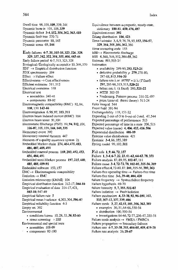
Index
Dwell time 98,108,109,339,341 Dynamic burn-in 101,109,339 Dynamic defect 3-4,152,354,362,363,410 Dynamic fault tree 270-71 Dynamic Parameter 88,145 Dynamic stress 69,144
Early failures 6-7,35,315-16,323,326,328, 329,337,342,352,354,355,406,445-46
Early failure period 6-7,315,323,328 Ecological IEcologically acceptable 10,369,370 EDF + Empirical distribution function EDX spectrometry 104 Effect + Failure effect Effectiveness -+ Cost effectiveness Efficient estimates 51 1,512 Electrical overstress 148 Electrical test
assemblies 340-41 . components 88-92 Electromagnetic compatibility (EMC) 82,84,
108,139,143-44 Electromigration 6,95,97,103,311 Electron beam induced current (EBIC) 104 Electron beam tester 91,104 Electrostatic Discharge (ESD) 89,94,102,104,
106-07,108,139,144,148,335 Elementary event 392 Elementary renewal theorem 447 Elements of a quality assurance system 21 Embedded Markov chain 274,464,475,483,
486,487,488,491 Embedded renewal process 169,203,452,453,
456,484,491 Embedded semi-Markov process 197,215,440,
485,488,489-91 Embedded software 153,157 EMC -+ Electrornagnetic compatibility Emission + EMC Emission microscopy (EMMI) 104 Empincal distribution function 3 12- 17,504-10 Empirical evaluation of data 314-17,421,
503-10,547-49 Empirical failure rate 5 Empirical mean I variance 4,303,304,506-07 Empincal reliability function 4-5 Empty set 392 Environmental . conditions lstress 10,28,33,36,82.83
stress screening -+ ESS Environmental and special tests
assemblies 108-09 . components 92-100
Equivalence between asymptotic, steady-state, stationary 180-81,450,476,487
Equivalent event 392 Erlang distribution 186,423 Error I mistake 3,6,9,76,78,95,153,156-57,
329,354,355,356,362,386 E m r correcting code 153 ESD -+ Electrostatic discharge ESS 6,341,349,352,35445,362 Estimate 511,503-24 Estimation
availability 289-90,293,523-24 defective probability p 279,278-80, 287-88,513,516-20 failure rate h or MTBF = I 1 h (T fmed) 297,295-98,513,515,520-21 failure rate h (k fixed) 295,521-22 MiTR 303-05 Nonhomog. Poisson process 33 l-32,497 pointlinterval (basic theory) 511-24
Euler integral 544 Event field 391-94 Exchangeability 118,151-52 Expanding 2-out-of-3 to I-out-of-3 red. 47,544 Expected percentage of performance 513 Expected percentage of time in a state 206,513 Expected value (mean) 4,406,415,416, 506 Exponential distribution 408-09 Extreme value distributions 421 Extrinsic 3-4,86,355,389 Eyring model 99,102,311
Faii-safe I, 9,66,72,157 Failure 1,3-4,6-7,22,23,61-62,64-65,78,355 Failure analysis 87,89,95,102-07,111 Failure cause 3-4,72-73,78,102-05,355-56,389 Failure effect 4,72-80,87,101,355-56,389,363 Failure-free operating time -+ Failure-free time Failure-free time 3-6,39-40,404,420 failure frequency -+ System failure frequency Failure hypothesis 69-70 failure intensity 5,7,355,501-02 Failure isolation -+ Fault isolation Failure mechanism 4,33-38,92,96-100,102,
103,307-12,337,339,406 Failure mode 3,27,42,51,101,356,362,389
examples 3O,5l, 64-66,550-54 distribution 100,550-54 investigations 64-66,72-77,236-47,255-58
Failure mode anaiysis + FMEA / FMECA Failure propagation + Secondary failures Failure rate 4-7,33-38,355,404-05,409,419-20 Failure rate analysis 26,28-67
Index
Failure rate confidence limits at components level 296-98 . at system level 298
Failure rate estimation 296-98,513,520-22 Failure rate demonstration 298-303 Failure rate models IHDBKs 35-38,99,310-12 Failure rate of mixed distributions 41,404-06 Failure recognition 101,116-18,149-51,236-46 Failures with constant failure rate h 6-7,35 False alarm 66,232,241,246 Fatigue 88,98,311,421 (see also Wearout) Fault 4,72,356 Fault coverage -t Incomplete coverage Fault isolation 116-17 Fault model 90,91,236-64 Fault modes and effects analysis -t FMEA Fault recognition 112,115,116-18,119,149 Fault tolerant system 47,64-65,66,101,153,
157,162,165,231,233,248-60,264,476,478 Fault tree /Fault tree analysis (FTA) 66,76,78,
270-71,356 Feasibility I feasibility check 10, 19,77,121,
154,354,378,381,383,384 Field of events 391-94 Fine leak test 339-40 Finite element analysis 69 First delivery 350 First-in / first-out 164,232,273 Fishbone diagram -+ Ishikawa diagram Fisher distribution 290,291,523,532,429,542-43 FIT (Failures in time) 36 Fitness for use 11,360 fixed length test -+ Simple two-sided test Flow of system failures 16 1,294,330,497 FMEAFMECA 27,42,66,69,72-75,78,117,
237,248,264,355,377 Force of mortality 7,356 Forward recurrence time 175,178,180,446-47,
448,45 1,454 (see also Rest waiting time) Frequency / duration 231,148,255,259-60,266,
475,476-78,487 FTA -t Fault Tree Analysis Functional block diagram 29,68,256,271 Function of a random variable 405,410,426 Functional test 88
Gamma distribution 408-09,422-23 Gamma function 544 Gate review 378,381 Gaussian distribution + Normal distribution General reliability data 3 19-28 Generation of nonhomog. Poisson processes 497 Generator for stochastic processes 275-76
Geometric distribution 408-09,431 Geometric probability 395,408-09,43 1 Glassivation + Passivation Glitches 66, 146 Glivenko-Cantelli theorem 505 Gold-plated pins 94,147 Gold wires 100 Good-as-new -+ As-good-as-new Goodness-of-fit tests 312-18,322,533-38 Graceful degradation 66,248 Grain boundary sliding 109,341 Grigelionis theorem 498 Gross leak 339-40 Ground 143-45,146,147,152 Guard rings 144,146 Guidelines -t Design guidelines
HALT 312 HAST 89,98-99,312 Hazard rate 5 HBM -t Human body model HPP -+ Poisson process (homogeneous PP) Hermetic enclosure 142,148 Hermetic package 85,102,104,142,337,339 Hidden defect 14,117 Hidden failures 8,66,79,107,113,116,117,120,
149,150,233,241-46,243,359 High temperature Storage 89,98,337 Higher-order moments 41 0,4 11,507 Highly accelerated tests 3 12 Historical development 16,17,85 Homogeneous -t Time-homogeneous Homogeneous Poisson process + Poisson proc. Hot carriers 96,102,103 Hot redundancy + Active redundancy Human aspects Ifactors 2,3,9,27,73,76,77,
152,153,157-58,352,361,363,373,385 Human body model (HBM) 94 Human errors 10,119,157 Human reliability + Risk management Humidity tests 89,98-100 (See also HAST) Hypergeometric distribution 408-09,432
Idempotency 61,392 Imperfect switching -t Switching In-circuit test 340 Inclusion / Exclusion 400 Incoming inspection 90,101,145,336,340,
343,344-49 Incomplete coverage 241-46,267 Independent elements 52 Independent events 397,398 Independent increments 439-40
Index
Independent random variable 394,413,415, 416,416-18,419,422,423,434,465
Indicator 56,57,58,61 Indices 167 Indirect plug connectors 152 Inductive Icapacitive coupling 91,143,146 Industrial applications (environment) 37,38,140 Influence of prev. maintenance 134-36,233-36 Influence of repair time distribution 114-15,
133-34,198-200 Information feedback 22,360-61,390 Infrared thermography (IRT) 104 Inherent + Intnnsic Initial conditions 63,176,178,180,190,191,
208,449-50,454-55,462,469,471,485 Initial distribution 449,459,460-61,463,
475-76,485,486-87,491-92 Input/output dnver 146 Inserted components 84,108,110 Integral equations (method of) 166,185,193-94,
211-12,216-17,473-74 Integral Laplace theorem 434,5 18 Integrated circuits (ICs) 34-37,84-85,89,
90-100,142,149,336,337-40 Intensity 7,296,321,451,493,497,498,501,502 Interaction 66,253,156 Interarrival time 5,294,319,323,328,442,494 Interchangeability 8 Interface 78,82,96,97,103,118,139,146,154,157 Intermetallic compound Ilayer 100,103,109 Internal redundancy + Active redundancy Internal visual inspection 89,93,104 Intersection of events 392 Interval estimation 278-80,289-90,293,296-98,
305,516-24 Interval estimate at system level 298 Interval reliability 166-67,172,177,181,188,
193,195,198,211,265,454 Intrinsic 3-4,9,86,139,355,389 Inverse function 405 Ion migration 103 Irreducible Markov chain 459-60,475-76,
486-87,491 IRT -;r Infrared thermography Ishikawa diagrarn 76-77,78,356 ISO 9000: 2000 family 11,366-67 Item 2,357
Jelinski-~oranda 160 Joint availability 174- 175,177 Joint density I distribution 412-13,494-95 Junction temperature 33,34,35,37,79,84,85,
140-42,145,309
k-out-of-n: G -+ k-out-of-n redundancy k-out-of-n redundancy 31,44,61-64,130,
206-12,211,225,227,271,479,489-90 Kepner-Tregoe 76,78 Key item method 52-55,60,68-69 Key renewal theorem 178,179,448,455,457,491 Khintchine theorem 45 1,498 Kirkendall voids 100 Kolmogorov backward / forward eqs. 462 Kolmogorov-Smirnov test 312-17,322,332,497,
534,536-37,543 Korolyuk theorem 493 kth momentkentral moment 410-1 1
Laplace test 324 Laplace transform 545-46 Last repairable unit + Line replaceable unit Last replaceable unit + Line replaceable unit Latch-up 89,96,145,148 Latent damage -+ Darnage Law of large numbers 433-34 Leak test + Seal test Liability + Product liability Life cycle cost (LCC) 11,13,16,112,353,357,
364,369,370,377 Life-cycle phases 19 (hardware), 154 (software) Lifetime 357 Like new + As-good-as-new Likelihood function + Max. likelihood function Limit theorems of probability theory 432-37 Line repairable unit -+ Line replaceable unit Line replaceable unit (LRU) 115,116,118, 120,
125,149 Liquid crystals 104 List of preferred parts (LPP) + Qualified part
list Load capability 33 Load sharing 43,45,52,61-64,163,164,190,
194,207,458,488 Logarithmic Poisson model 333 Logistic support 8,115,119,125,129,235,357 Lognormal distribution 113-15,303-07,408-09,
425-26,547 Long-term stability 86 Lot tolerance percent defective 284-85,530 Lowest replaceable unit + Line replaceable unit LRU + Line replaceable unit LTPD + Lot tolerance percent defective
Macro-structures 165,222,227,264 Maintainability 1,2,8, 9,12,13,21,112-15,
357,366,367,368

Index
Maintainability analysis 72,115-24,149-52, 373,375
Maintainability estimation/demonstr. 303-07,371 Maintainability program -t Maintenance concept Maintenance 8,113 Maintenance concept 8,112,115-20,373,375 Maintenance levels 119-20 Maintenance strategy 35,134-36,233-36 Majority 31,47,66,215 Manufacturing processes 106-1 1,147-48,335-
50,378 Manufacturing quality 16,20,86,335-50 Margin voltage 98 Marginal density I distribution function 413 Marking 306 Markov chain 244,268,274,458-60,461,463,
464,475,483,485,486,487,488 Markov models 61-64,166-67,170-71,189-93,
195,211,220-21,225,227,226-30,238-40, 260-63,264-67,440,460,466-68,471,479
Markov process 166-67,440,460-83,487 Markov renewal property 465
(see also Memoryless property Markov renewal processes 483 Match IMatching 144,146 Mathematical statistics 503-38 Maximum likelihood function lmethod 278,89,
296,304,305,313,319,322,331,512-15,536 Mean (expected value) 406-07,410,415,416 Mean down time (MDn 124,259,266,478 Mean (for rel. applications) -+ MDT, MTBF,
MTBUR, MTTF, MTTPM, MTTR, MUT Mean logistic delay 235 Mean operating time between failures (MTBF)
6,39-40,358 (see also 294-303,369-71 for estimation & demonstration of MTBF=l I h)
Mean time to failure (M77'fl 6,39,40,63,166- 67,195,211,220-21,225,227,358,474,486
Mean time to preventive maintenance ( M Z P M ) 113,121,125,358
Mean time to repair (MTTR) 8-9,113,121-24, 359 (303-07 for estimation & demonstration)
Mean time to restoration -+ Mean time to repair Mean up time 6,265,477 Mean value function 321,324,328,333,493,496 Mechanical reliability 67-7 1 Mechanism -+ Failure mechanism Median 412 Meshed structure 52 Memories 90-91,93,97-98,146 Memoryless property 7,40,63,136,172,192,234,
2!?5,298,405,420,43l, 440,451,464,465,478 Meta1 migration 103 (see also Electromigration)
Metallographic investigation 104-05,108-09 Method of differential eqs. 167,190-81,469-72 Method of integral eqs. 166,193-94,473-74,486 Metrics (software quality) 153 Microcracks + Cracks Microsection 104,105,108,110 Minimal cut sets 59,60,76 Minimal operating state -t Critical Oper. states Minimal path Sets 58,60,76 Mission availability 173 Mission profile 3,15,28,38,68,79,231,357,370 Mistake -+ Error Mixed distribution function 403 Mixture of distributions 7,41,316,406 Modal value 412 Mode -+ Failure mode Models for failure rates 35-38 (see also Mixture) Models for faults -+ Fault model Modification 379 Moisture 98-99,142 Module I Modular Il8,120,149,150-59 Moment generating function 545 Monotony 57 Monte Carlo simulation l65,23 1,233,272,
273-76,426,435,436 (see also Generation and Generator)
Motivation and training 24,119,375 MDT -+ Mean down time MTBF -+ Mean operating time between failures MTBUR 8,358 MTTF + Mean time to failure MZTPM -+ Mean time to prev. maintenance MTTR + Mean time to repair / restoration MUT -+ Mean up time
Multidimensional random var. 412- 16,438-41 Multifunction system -+ Phased-rnission system Multilayer 143,148 Multimodal 412 Multinornial distribution 318,429,537,538 Multiple failure mechanism 64-65,310,3 12,
319,341,406 Multiple failure mode 52,64-65,66,246-47,
255-58 Multiple faults I consequences 76 Multiple one-sided sampling plans 285-86 Multiplication theorem 398-99 Mutually exclusive events 57,171,174,237,
392,393,394,397-98,400,446 MUX 150,151
Nitride passivation -+ Passivation Nonconformity 354,359 Nondestructive analysis 102-05
Index
Nonhomogeneous Poisson process 161,321-34, 451,493-97
Nonregenerative state 201,210,440,490 Nonregenerative stochastic process 164,186,
200,212,488,492-502 Nonrepairable item (up to system failure) 5,7,
39-57,61-71,236-37,240,243,245,254,260, 270,272
Normal distribution 113,126-127,408-09, 424-25,434-35,449,496,539,549
Number of states 56,219 N-version programming (NVP) 47
OBIC 105 Object oriented programming 157 Observability 149 Obsolescence 8,118,138,145,357 Occurrence time + Arrival time One-item structure 39-41,168-82
Parameter estimation 278-80,289-90,293, 294-98,303-05,331-32,511-24
Pareto 76,78 Part Count method 5 1 Part Stress method 33-38,50-51 (see also 69-71) Partitioning 115,118,157,158 Partitioning cumulative operating time 294,
295,301,371 Passivation IPassivation test 89,93,104,106 Path Set -+ Minimal path sets Pattern sensitivity 91,93 PCBs + Populated printed circuit boards Pearson 517,535 Percentage point 412 Performability 259 Performance -+ Capability Performance effectiveness + Reward Performance test 108 Petri nets 267-69
One-out-of-2 redundancy ( 1-out-of-2 redundancy) Phased-mission Systems 28,30,38,231,248-55 42-43,189-206,225,227,236-45,247,260-64, 466,470-72,488-92
One-sided confidence intervai 280,290,297, 316,319,321,322,324,516,519
One-sided sampling plan (forp) 284436,529-30 One-sided tests to demonstrate kor MTBF=1 I k
302-03 Only one repair Crew + models of Chapter 6 except pp. 210,224-25
Operating characteristic lcurve 281-82,284-85, 300,306-07,527-28,530
Operating conditions 2,3,7,26,28,33,35,79, 84,90,96,99,102,354,365
Operation monitoring 116 Operational availability 235 Operational profile 28 Optical beam induced current (OBIC) 104 Optimal derating 33,140 Optimal preventive maintenance 234-36,242-43 Optimization l2-l5,67,l2O,l36,l38,342-49,
353,364 Optocoupler 146 Order observations 1 sample lstatistics 3 12,3 13,
321,323,324-25,332,495,496,5O4,5O6,535 Organizational structure (company) 20 Overall availability 9,235 Overstress 33,103,148,336 Oxide breakdown 96-97,102,103,106,3 11
Packaging 84-85,89,100,142 Parallel model 43-45,61-64,195,206,211,225,
227,236-43,247,466-39,470-42,489,490 Parallel redundancy + Active redundancy
~h~sics-of-failures 102-07 (see Failure mech.) Pitch 84,109,147,341 Plastic packages -i Packaging Point availability 9,170,178,181,166-67,190,
289-93,352,454 Point estimate 278,289,296,303,332,511-15 Point estimate at system level 298 Point process (general) 500-02 Poisson approximation 430 Poisson distribution 283,294,408-09,429-30 Poisson integral 544 Poisson process
homogeneous (HPP) 7,294,295-96,320, 323-27,356,445,448,450-51,515, 493-97 for m(t)=h nonhomogeneous (NHPP) 161,3Sl-34,451, 493-97
Populated printed circuit board (PCB) 84,85,90, 94,107-11,116,144,146-48,152,336,340-41
Power devices 1 supply 96,98,99,108, 143, 145,146,147,150,152
Power Law process 230 ppm 337,424 Precision measurement unit (PMU) 88 Predicted maintainability 121-25 Predicted reliability 3,25-27,28-71,172-276,
372 Preferred list -+ Qualified part list (QPL) Preheating 147 Preliminary design reviews + Design reviews Pressure cooker -+ HAST Preventive action 16,22,72,77,112,139-52,
155-58,341,37 1-82
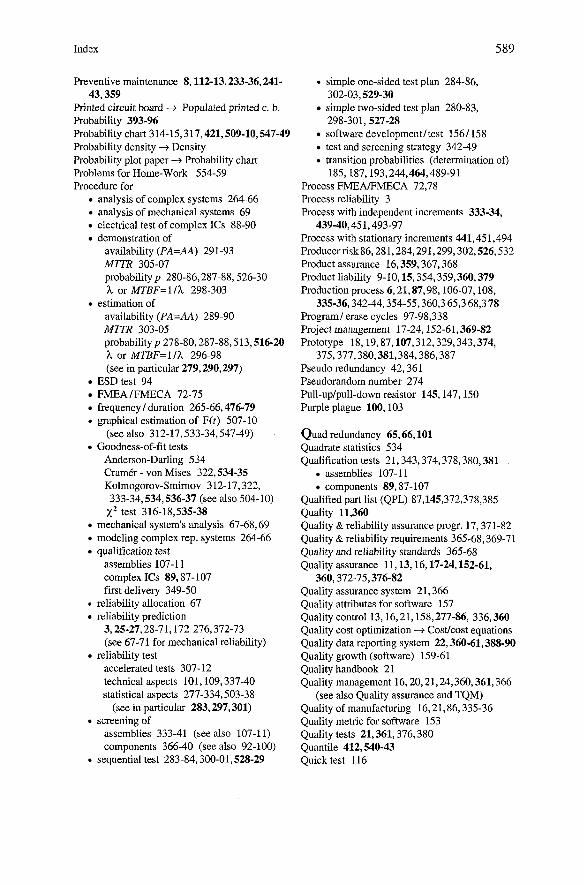
Index
Preventive maintenance 8,112-13,233-36,241- 43,359
Printed circuit board -+ Populated printed C. b. Probability 393-96 Probability chart 314-15,317,421,509-10,547-49 Probability density + Density Probability plot paper -t Probability chart Problems for Home-Work 554-59 Procedure for
analysis of complex systems 264-66 analysis of mechanical systems 69 electrical test of complex ICs 88-90 demonstration of
availability (PA=AA) 291-93 MTTR 305-07 probability p 280-86,287-88,526-30 li. or MTBF= 1 Ili. 298-303
estimation of availability (PA=AA) 289-90 MTTR 303-05 probability p 278-80,287-88,513,516-20 h or MTBF= 1 Ih 296-98 (see in particular 279,290,297)
ESD test 94 FMEAIFMECA 72-75 frequency I duration 265-66,476-79
0 graphical estimation of F(t) 507-10 (see also 312-17,533-34,547-49)
Goodness-of-fit tests Anderson-Darling 534 Cramer - von Mises 322,534-35 Kolmogorov-Smimov 3 l2-17,322, 333-34,534,536-37 (see also 504-10) X* test 316-18,535-38
mechanical system's analysis 67-68,69 modeling complex rep. systems 264-66 qualification test
assemblies 107-1 1 complex ICs 89,87-107 first delivery 349-50
reliability allocation 67 reliability prediction
3,25-27,28-7 l,l72-276,372-73 (see 67-71 for mechanical reliability)
reliability test accelerated tests 307-12 technical aspects 101,109,337-40 statistical aspects 277-334,503-38
(see in particular 283,297,301) screening of
assemblies 333-41 (see also 107-1 1) components 366-40 (see also 92-100)
sequential test 283-84,300-01,528-29
s simple one-sided test plan 284-86, 302-03,529-30 simple two-sided test plan 280-83, 298-301,527-28 software developmentltest 1561158 test and screening strategy 342-49 transition probabilities (determination of) 185,187,193,244,464,489-91
Process FMEAIFMECA 72,78 Process reliability 3 Process with independent increments 333-34,
439-40,451,493-97 Process with stationary increments 441,45 1,494 Producer risk86,28 1,284,291,299,302,526,532 Product assurance 16,359,367,368 Product liability 9-10,15,354,359,360,379 Production process 6,21,87,98,106-07,108,
335-36,342-44,354-55,360,3 65,3 68,3 78 Programl erase cycles 97-98,338 Project management 17-24,152-61,369-82 Prototype 18,19,87,107,312,329,343,374,
375,377,380,381,384,386,387 Pseudo redundancy 42,361 Pseudorandom number 274 hll-uplpull-down resistor 145,147,150 Purple plague 100,103
Quad redundancy 65,66,lOl Quadrate statistics 534 Qualification tests 21,343,374,378,380,381
assemblies 107-1 1 components 89,87-107
Qualified part list (QPL) 87,145,372,378,385 Quality 11,360 Quality & reliability assurance progr. 17,371-82 Quality & reliability requirements 365-68,369-71 Quality and reliability standards 365-68 Quality assurance 11,13,16,17-24,152-61,
360,372-75,376-82 Quality assurance system 21,366 Quality attributes for software 157 Quality control 13,16,21,158,277-86, 336,360 Quality cost optimization + CostJcost equations Quality data reporting system 22,360-61,388-90 Quality growth (software) 159-61 Quality handbook 21 Quality management 16,20,21,24,360,361,366
(see also Quality assurance and TQM) Quality of manufacturing 16,21,86,335-36 Quality metric for software 153 Quality tests 21,361,376,380 Quantile 412,540-43 Quick test 116
Index
Random duration (phased-mission systems) 274 Repair priority 214,227,229,232,239,240,247, Random sample + Sample 256,264,466,468 Random variable 401-03 Repair rate 115,170-71,177,214,466,468 Random vector 412-15,438-41 Repair strategy -+ Maintenance strategy Rare event 10,272,273,275 Repair time 8,113-14,121-24,303-07,359 Reachability tree 268-69 Repairable spare parts -t Spare parts Reconfiguration 66,118,157,231,248-60 Repairable Systems 5,162-276
time censored (phased-mission system) 248-55 Repairable versus nonrepairable 40 failure censored 255-58 Repairability + Corrective maintenance with reward and frequencylduration 259-60 Replaceability 152
Recrystallization 109 Replacement policy 236 Recurrence time 174,175,178,446-51,494 Requalification 87 Recycling 10,19,357 Required function 28,362 Redesign 8,329 Requirements + Quality and rel. requirements Reduction (diagram of transition rates) 264(P.2) Reserve contacts 152 Redundancy 42-45,47,51,61-64,65,66,68,189- Reserve/reserve state 43,62,163,190,201
92,195,211,220-21,225,227,236-46,260-64, Rest waiting time 221,494 361 Restart anew 171,440,456 in software 47,153,157 Restoration 8,112,353
Reflow soldering 147 Restoration frequency -t System repair freq. Refuse to start 239 Results (tables lgraphs) 31,44,48-49,111,127, Regeneration 1 renewal point 201,440,442, 166-67,177,181,188,195,206,211,220-21, 453,456,473,484,489,490 225,227,230,234,258,279,283,290,292,297,
Regeneration state 200,215-16,440,456,464, 301,302,309,315,408-09,45 1,468,s 10,522 484,489 Reuse 10,116,119,130
Regenerative process 456-57 Reward 23 1,255,259-60,266,476,478-79 Rejection line 283-84,301-02,528-229 Rework 108,148,341 Relation between 4 and Pi 475 Rise time 143,144
(see also Distinction between) Risk 9-11,15,67,72,145,148,273,278,347, Relative frequency 278-789,393,394-96,513,516 363,369,373,384 Relaxation 109 (see a, ß & ß, , ß2, y for statistical nsk) Reliability 2,13,27,66,69,72,231,361,367,372 ROCW 542 Reliability allocation 67 Rules for Reliability analysis 13,25-27,66,67-71,80, convergence PA(t ) + PA 179-80,195
139-48,162-67,372-73,377-78 data analysis 320 Reliability block diagram (RBD) 28-32,68-69,362 derating 33,140
(see 23 1-76 if the RBD doesn't exist) FMEA/FMECA 72 Reliability function 2-3,166-67,169,176,361, imperfect switching 238,240,247 404,471-72,473-74,486 incomplete coverage 245
Reliability growth 329-34,362 (see also 159-61) jnnction temperature 37,141,145 Reliability prediction + Procedure for partition of cumulative operating time Reliability tests + Procedure for 294,295,301,371 Remote control ldiagnostic 117-18,120 power-up 1 power-down 145,147 Renewal density 443-44 quality and reliability assurance 19 Renewal density theorem 179,448 senes /parallel structures 46,219 Renewal equation 444 (see also Design guidelines ) Renewal function 443 Run-in 341,352 Renewal point + Regeneration point Renewal process 164,441-51 Safety 9-10,13,15,66,72,78,362-63,366,379 . embedded 203,452-52,456,484,487,491 Safet~ anal~sis 15,66,72-78,373,377,378 Repair 8,113,163-64,353,359 Safety factor 69 Repair frequency -t System repair frequency Same element in rel. bleck diagram 30,32,55,
60.69
Index
Same stress 45,71 Sample 504 Sample space 391-92 Sampling tests 277,280-88,34449,527-30 Scan path 150-5 1 Scanning electron microscope (SEM) 104 Schmitt-trigger 92,143 Scrambling table 91 Screening (see also ESS)
assemblies 340-41 components 337-340 (see also 92-100)
Screening strategy -+ Test and screening strategy Seal test 339-40 Secondary failure 4,66,73 Selection cnteria for electronic comp. 550-53 Semidestructive analysis 104 Semi-Markov process 164,166-67,440,483-88 Semi-Markov proc. embedded -+ Semi-reg. proc. Semi-Markov transition probability 166,185,
187,197,244,463-64,48445,489,490 Semi-regenerative process 162,163,164,197,
215,233,264,273,274-75,438,440,488-92 Sequential test 283-84,300-02,528-29 Senes model 41-42,64,71,182-88,320,406,421 Series - parallel structure 45-49,213-30,468
(see 48-49 and 220-21 for comparisons) Series - parallel system -+ Seties- paral. structure Serviceability i, Preventive maintenance Services reliability 3 Set operations 392 Shewhart cycles 76 Shielded enclosure 144 Shmoo plot 9l,93 Short-term test 312 Silicon nitride glassivation -t Passivation Simple one-sided test 284-86,302-03, 529-30 Simple structure 28,39-5 1,168-236 Simple two-sided test 280-83, 298-301,527-28 Simulation -+ Monte Carlo Single-point failure 42,66,79 Single-point ground 143 Six-o approach 424 Sleeping state -+ Dormant state SMD I SMT 84,109-11,146-47,341 Sneak analyses 76,79,377 Soft error 97 Software
attributes + quality attributes defects 67,117,149,152-53,155-61,329 defect prevention 155-58,160 design reviews 154,157,158,159 development procedure 153-56 documentation 154,155,156
FMEAFMECA 72-73 interaction 156 life-cycle phases 154 metncs 153 quality assurance 21,152-61,153,362 quality attributes 153,155 quality metrics 153 quality growth 159-61,329-334 specifications 154,156,157,159 standards 143,152,153,158,159 testing I validation 158-59 time lspace domain 153,157
Sojoum time i, Stay time Solder joint 84-85,108-11,147,340-41 Solder-stop pads 146,147 Solderability test 94 Soldering temperature profile 147,148 Spare parts provisioning 125-34 Special diodes 145 Special manufacturing processes 378 Specifications 3,154,156,157,159,365,372,
376,379,381,386 Standard deviation 41 1 Standard industrial environment 36 Standard normal distribution 424-25,539 Standardization 117,120,149,152,155,365,386 Standards 365-68 Standby redundancy 43,62,195,206,
211,237,361,418 (see also Active &Warm) State probability 63,190,461,475-76,486-87 State space 438-41 State space extension 492 State space method 56-57 State space reduction 264 State transition diagram -+ Diagram of Static fault tree 270 Stationary (or in steady-state)
alternating renewal process 180-81,454-55 distribution 459,475,486,488 increments (time-hoinogeneous) 441 initial distribution 459,475,486,488 Markov chain 459 Markov process 166-67,474-76,488 one-item structure 180-81 process 440-41 regenerative process 457 renewal process 449-51 semi-Markov process 166-67,486-8s
Statistical decision 504 Statistical error -+ Statistical risk Statistical hypothesis 525-26 Statistical maintainability tests 303-307 Statistical quality control 16, 277-86
Index
Statistical reliability tests 277-334,503-38 Statistical risk 503 (see also a, P, ßl, ßz, Y) Statistically independent 397,504,512,525
(see also Stochastically independent) Statistics + Mathematical statistics Status test 116,119 Stay time (sojourn time) 163,166-67,249,264,
274,275,458,463-64,474,479,483,486,488 Steady-state + Stationary Steady-state property of Markov processes
477,480,488 Step-stress tests 3 12 Strategy
maintenance 35,134-36,233-36 . test&screening 342-44,347-49,361,373,380 Stirlings' formula 3 19,544 Stochastic demand 174 Stochastic matrix 458,460 Stochastic process 438-41,441-502 Stochastically independent 397,399,413 Storage temperature 148 Stress factor 33,139-40,145 Stress-strength method 69-71,76 Strict liability 15,360 Strong law of large numbers 434,505 Structure function -+ System function Stuck-at-state 238,247 90 Stuck-at-zero 1 at-one 90 Student distribution 541 Successful path method 55-56 Sufficient statistic 295,324-27,511-12,513,514 Sum of
Homogen. Poisson proc. 296,451,498 Nonhomogen. Poisson proc. 45 1,496,498 Point processes 501 Random variables 416-18,443 Renewal processes 497-98
Superconform 535 Superimposed processes -+ Sum of Superposition + Sum of Supplementary states 186-88,492 Supplementary variables 186,492 Suppressor diodes 143,144 Surface mount devices I techn. -+ SMD 1 SMT Survival function -+ Reliability function Susceptibility + EMC Sustainable development 10,357,385 Switch 47,48-49,213-19,220-21,236-40,255-58 Switching + Switch System 2,31,166-67,264-66,363 System's confidence limits 298 System design review 381,383-87 System effectiveness + cost effectiveness
System failure frequency 265-66,477-78 System function 58 System mean time to failure (M7TFS )+ MTTF System reconfiguration -+ Reconfiguration System repair kequency 266,478 System restoration frequency + System rep. freq. System specifications + Specifications Systems engineering 1 1,16,357,363 Systems with complex structure 31,52-67,69,
231-33,236-76 Systems with hardware and software 161 System without redundancy + Senes model Systematic failure 1,3,6,109,115,329,331,342,
352,354,355,362,363
Tasks / task assignment l7-20,372-75 Technical Availability 235 Technical safety + Safety Technical system -+ System Tecbnological characterization 96-98 Technological properties Ilimits 10,38,84-85,
92,96-100,107-111,550-54 Test and screening procedures + Screening Test and screening strategy 342-44,347-49,361,
373,380 (see also Screening) Test coverage 90,91,117,231.233,241-46 Test Pattern 90-93 Test plan 281,283,291,292,299,301,306,527,
528,529-30,532 Test point 147,150 Test time partitioning + Partitioning Test vector 88 Testability 117,147,149-51,155,157,158 Testing
unknown availability 291-92,293,531-32 unknown distr. function 312-18,533-38 . unknown MTTR 305-07
0 unknown probability 28046,287,291- 92,526-30,531-32 unknown h or MTBF=l I h 298-303, statistical hypotheses (basic theory) 525-38
Tchebycheff 4 Chebyshev Theorem of cut sets + Cut sets theorem Thermal cycles 83,95,98,100,108,109,110,
337-39,341 Thermal design concept / management 141 Thermal resistance 141-42 Thermal Stress 145 Three Parameter Weibull disturb. 421,509-10 Time censoring -+ Censoring Time-dep. dielectric breakdown 96-97,103 Time-homogeneous Markov process 164,166-
67,440,460-83
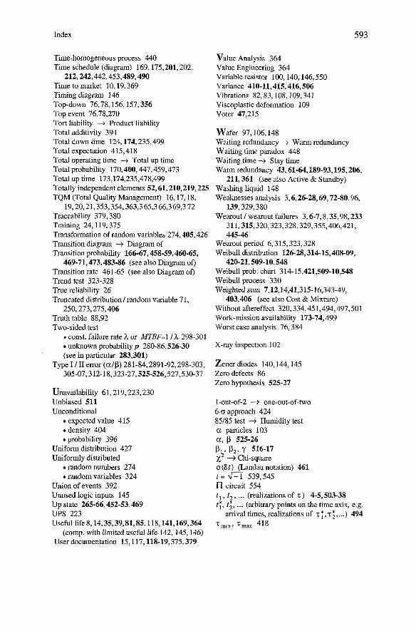
Index
Time-homogeneous process 440 Time schedule (diagram) 169,175,201,202,
212,242,442,453,489,490 Time to market 10,19,369 Timing diagram 146 Top-down 76,78,156,157,356 Top event 76,78,270 Tort liability + Product liability Total additivity 394 Total down time 124,174,235,499 Total expectation 415,418 Total operating time -+ Total up time Total probability 170,400,447,459,473 Total up time 173,174,235,478,499 Totally independent elements 52,61,210,219,225 TQM (Total Quality Management) 16,17,18,
19,20,21,353,354,363,3 65,3 66,369,3 72 Traceability 379,380 Training 24,119,375 Transformation of random variables 274,405,426 Transition diagram + Diagram of Transition probability 166-67,458-59,460-65,
469-71,473,483-86 (see also Diagram of) Transition rate 461-65 (see also Diagram of) Trend test 323-328 True reliability 26 Truncated distnbution / random variable 71,
250,273,275,406 Truth table 88,92 Two-sided test . const. failure rate h or MTBF=I l h 298-301
unknown probability p 280-86,526-30 (see in particular 283,301)
Type I I I1 error (alß) 281-84,2891-92,298-303, 305-07,312-18,323-27,525526,527,530-37
Unavailability 61,219,223,230 Unbiased 511 Unconditional
expected value 415 density 404 probability 396
Uniform distribution 427 Uniformiy distributed
random numbers 274 random variables 324
Union of events 392 Unused logic inputs 145 Up state 265-66,452-53,469 UPS 223 Useful life 8,14,35,39,81,85,118,141,169,364
(comp. with limited useful life 142, 145,146) User documentation 15,117,118-19,375,379
Value Analysis 364 Value Engineering 364 Variable resistor 100,140,146,550 Variance 410-11,415,416,506 Vibrations 82,83,108,109,341 Viscoplastic deformation 109 Voter 47,215
Wafer 97,106,148 Waiting redundancy + Warm redundancy Waiting time paradox 448 Waiting time -t Stay time Warm redundancy 43,61-64,189-93,195,206,
211,361 (see also Active & Standby) Washing liquid 148 Weaknesses analysis 3,6,26-28,69,72-80,96,
139,329,380 Wearout / wearout failures 3,6-7,8,35,98,233
31 l,315,32O,323,328,329,355,4O6,421, 445-46
Wearout period 6,315,323,328 Weibull distribution 126-28,314-15,408-09,
420-21,509-10,548 Weibull prob. chart 314-15,421,509-10,548 Weibull process 330 Weighted sum 7,12,14,41,315-16,343-49,
403,406 (see also Cost & Mixture) Without aftereffect 320,334,451,494,497,501 Work-mission availability 173-74,499 Worst case analysis 76,384
X-ray inspection 102
Zener diodes 140,144,145 Zero defects 86 Zero hypothesis 525-27
1-out-of-2 -+ one-out-of-two 6-0 approach 424 85/85 test + Humidity test a particles 103 a, ß 525-26 ßy 02, Y 516-17 X -+ Chi-square o (6t) (Landau notation) 461 i = 539,545
circuit 554 t t (realizations of z ) 4-5,503-38 " 2 ' " ' tl;, t2, ... (arbitrary points on the time axis, e.g.
arrival times, realizations of z T, T 2, ...) 494 7,n, T„, 418


