A GPU-Based Implementation of the Firefly Algorithm for Variable Selection in Multivariate Calibration Problems

RESEARCH ARTICLE

A GPU-Based Implementation of theFirefly Algorithm for Variable Selection inMultivariate Calibration ProblemsLauro C. M. de Paula1, Anderson S. Soares1*, Telma W. de Lima1,Alexandre C. B. Delbem2, Clarimar J. Coelho3, Arlindo R. G. Filho4

1. Institute of Informatics, Federal University of Goias - UFG, Goiania, GO, Brazil, 2. Institute of MathematicalSciences and Computing, University of Sao Paulo - USP, Sao Carlos, SP, Brazil, 3. Computer ScienceDepartment, Pontifical Catholic University of Goias - PUC Goias, Goiania, GO, Brazil, 4. Department ofSystem and Control, Technological Institute of Aeronautics - ITA, Sao Jose dos Campos, SP, Brazil

*[email protected]

Abstract

Several variable selection algorithms in multivariate calibration can be accelerated

using Graphics Processing Units (GPU). Among these algorithms, the Firefly

Algorithm (FA) is a recent proposed metaheuristic that may be used for variable

selection. This paper presents a GPU-based FA (FA-MLR) with multiobjective

formulation for variable selection in multivariate calibration problems and compares

it with some traditional sequential algorithms in the literature. The advantage of the

proposed implementation is demonstrated in an example involving a relatively large

number of variables. The results showed that the FA-MLR, in comparison with the

traditional algorithms is a more suitable choice and a relevant contribution for the

variable selection problem. Additionally, the results also demonstrated that the FA-

MLR performed in a GPU can be five times faster than its sequential

implementation.

Introduction

Multivariate calibration refers to construction procedure of a mathematical model

that establishes the relationship between the properties measured by a instrument

and the concentration of a sample to be determined [1]. The building of a model

from a subset of explanatory variables usually involves two conflicting objectives:

N Extracting as much information from a measured data with many possible

independent variables;

OPEN ACCESS

Citation: de Paula LCM, Soares AS, de Lima TW,Delbem ACB, Coelho CJ, et al. (2014) A GPU-Based Implementation of the Firefly Algorithm forVariable Selection in Multivariate CalibrationProblems. PLoS ONE 9(12): e114145. doi:10.1371/journal.pone.0114145

Editor: Shyamal D. Peddada, National Institute ofEnvironmental and Health Sciences, United Statesof America

Received: November 18, 2013

Accepted: November 3, 2014

Published: December 10, 2014

Copyright: � 2014 de Paula et al. This is anopen-access article distributed under the terms ofthe Creative Commons Attribution License, whichpermits unrestricted use, distribution, and repro-duction in any medium, provided the original authorand source are credited.

Funding: The authors thank the research agen-cies CAPES, FAPEG, FAPESP and CNPq for thesupport provided to this research. This is also acontribution of the National Institute of AdvancedAnalytical Science and Technology (INCTAA)(CNPq - proc. no. 573894/2008-6 and FAPESPproc. no. 2008/57808-1). The funders had no rolein study design, data collection and analysis,decision to publish, or preparation of the manu-script.

Competing Interests: The authors have declaredthat no competing interest exist.

PLOS ONE | DOI:10.1371/journal.pone.0114145 December 10, 2014 1 / 22

http://crossmark.crossref.org/dialog/?doi=10.1371/journal.pone.0114145&domain=pdf

http://creativecommons.org/licenses/by/4.0/

N Decreasing the cost of obtaining data by using the smallest set of independent

variables that results in a model with high accuracy and low variance.

The balance between these two commitments is achieve using variable selection

techniques. The application of multivariate calibration had a breakthrough and

nowadays are very popular [2]. One of the most interesting features of modern

instrumental methods is the number of variables that can be measured in a single

sample. Recently, devices as spectrophotometers have generated large amount of

data with thousands of variables. As a consequence, the development of efficient

algorithms for variable selection is important in order to deal with data even

larger [3–5]. Furthermore, a high-performance computing framework can

significantly contribute to efficiently construct an accurate model [6]. In this

context, this paper presents an implementation of a modified Firefly Algorithm

(FA) for variable selection in multivariate calibration problems [4, 7, 8]. The FA is

a metaheuristic inspired by the flashing behaviour of fireflies [9].

Several works have used FA to solve many types of problems. For instance,

Yang [10] provided a detailed description of a new FA for multimodal

optimization applications. Lukazik and Zak [11] provided an implementation of

the FA for constrained continuous optimization. Yang [12] showed the use of the

FA for nonlinear design problems. Senthilnath et al. [13] used the FA for

clustering on benchmark problems and compared its performance with other

nature-inspired techniques. Gandomi et al. [14] used the FA for mixed-

continuous and discrete-structural optimization problems. Jati et al. [15] applied

the FA for travelling salesman problem. Banati and Monika [16] proposed a new

feature selection approach that combines the Rough Set Theory with the nature-

inspired FA to reduce the dimensionality of data containing large number of

features. Horng [17] proposed a new method based on the FA to construct the

codebook of vector quantization for image compression. Finally, Abdullah et al.

[18] introduced a new hybrid optimization method incorporating the FA and the

evolutionary operation of the differential evolution method. In all these works, the

experimental results showed that the FA scores over other algorithms in terms of

computing time and optimality.

This paper also uses a Graphics Processing Unit (GPU) to parallelize the

computation of the vector of regression coefficients in the problem of Multiple

Linear Regression (MLR). GPUs can be employed to improve performance of

computing applications usually handled by a Central Processing Unit (CPU) [5].

Husselman and Hawick [19, 20] are the only works we have found so far that

present a GPU-based implementation of a FA. Moreover, estimates from the

proposed FA (FA-MLR) are compared with predictions from the following

traditional algorithms: Successive Projections Algorithm for MLR (SPA-MLR)

[7], Genetic Algorithm for MLR (GA-MLR) [21, 22], Partial Least Squares (PLS)

[23] and Bayesian Variable Selection (BVS) [24]. In addition, it is used three

others criterions to determine the predictive ability of MLR models. The

generalization ability of the models is also evaluated by adding artificial

measurement noise to the independent variables.

GPU-Based Implementation of the Firefly Algorithm


The remaining of the paper is organized as follows. Section ‘‘Background’’

describes the multivariate calibration problem, the multicollinearity and variable

selection problems, and the original FA. The FA-MLR and the processing on a

GPU are presented in Section ‘‘The FA for Variable Selection’’. Section ‘‘Materials

and Methods’’ describes the material and methods used in the experiments.

Results are discussed in Section ‘‘Results and Discussion’’. Finally, Section

‘‘Conclusion’’ shows the conclusions of the paper.

Background

Multivariate Calibration

The multivariate calibration model provides the value of a quantity y based on

values measured from a set of explanatory variables fx1,x2, . . . ,xkgT[25, 26]. The

model can be defined as:

y~b0zb1x1z:::zbkxkz", ð1Þ

where b0, b1,…, bk, i51, 2,…, k, are the coefficients to be determined, and " is a

portion of random error.

A simple model to obtain the coefficients in Equation (1) based on calculation

of partial least squares is known as MLR, which is a statistical technique used to

build models describing reasonably relationships between several explanatory

variables of a given process [27, 28]. This technique requires the number of

observations greater than the number of variables. Nevertheless, the opposite may

occur for some applications (more variables than samples) [8]. For instance, in

problems involving spectrometric determination of a physical or chemical

quantity the explanatory variables correspond to measurements taken at various

wavelengths [29].

Equation (2) shows how the regression coefficients may be calculated using the

Moore-Penrose pseudoinverse [30]:

b~(XT X){1XT y, ð2Þ

where X is the matrix of samples and independent variables (collected by

instruments used for construction of multivariate calibration models), y is the

vector of dependent variables (or property of interest obtained in laboratory,

which serves as a parameter for model calibration), and b is the vector of

regression coefficients.

As shown in Equation (3), predictive ability of MLR models comparing

predictions with reference values for a test set from the squared deviations is

calculated by Root Mean Squared Error of Prediction (RMSEP):

RMSEP~

ffiffiffiffiffiffiffiffiffiffiffiffiffiffiffiffiffiffiffiffiffiffiffiffiffiffiffiffiffiPNi~1 (yi{yi)

2

N

s, ð3Þ



where y is the reference value of the property of interest, N is the number of

observations, and y~fy1,y2, . . . ,ykgTis the estimated value calculated as:

y~Xb: ð4Þ

Another criteria to determine the predictive ability of MLR models that has been

used is the Mean Absolute Percentage Error (MAPE) [31]. MAPE is a relative

measure which express errors as a percentage of the actual data and is defined as:

MAPE~

Pj yi{yi

yij

N(100)~

Pj ei

yij

N(100), ð5Þ

where yi is the actual data at variable i, yi is the forecast (using some model/

method) at variable i, ei is the forecast error at variable i, and N is the number of

observations (or samples) used in computing the MAPE.

The biggest advantage of MAPE is that it provides an easy and intuitive way of

judging the extent (or the importance) of errors. Furthermore, percentage errors

are part of the every day language making them easily and intuitively interpretable

[31]. This measure is widely used in forecasting as a basis of comparison. It can be

used to measure how high or low are the differences between the predictions and

actual data in regression models in a similar way to forecasting problems.

In statistics, there is also a technique called Predicted Residual Sums of Squares

(PRESS) proposed by Allen [32]. PRESS is a useful statistic for comparing

different models and is based on the leave-one-out technique [33]. It is also

known as a form of cross-validation used in regression analysis to provide a

summary measure of the fit of a model to a sample of observations that were not

themselves used to estimate the model [32]. The PRESS also may be used as a

measure of predictivity to compare and select the best model. However, one of the

main problems of cross-validation techniques is their computational cost, which

may become extremely higher and unviable [34]. Equation (6) shows how the

PRESS is calculated:

PRESS~XN

i~1

(yi{yi)2, ð6Þ

where y is a real value of concentration obtained by laboratorial methods, y is the

result of Equation (4) applied to measures of new observations (X measures), and

N is the number of observations.

Multicollinearity Problem and Variable Selection

In prediction problems with regression model having many variables, most of

them may not contribute to improve prediction precision. The selection of a

reduced set with variables that positively influence in the regression model is

important in order to improve the efficiency of algorithms for construction MLR

models. Moreover, the identification of a small set of variables that are



explanatory is usually desired in regression problems [3]. The problem of

determining an appropriate equation associated to a subset of independent

variables depends on the criteria used to: i) analyze the variables, ii) select the

subset and iii) estimate the coefficients in Equation (2).

There are some model (or variable) selection criterias in the literature [35]. An

approach is the use of information criteria such as Akaike Information Criteria

(AIC) proposed by Akayke [36] or the Bayesian Information Criteria (BIC)

proposed by Schwarz [37]. Equation (7) and (8) show how AIC and BIC may be

calculated, respectively:

AIC~ ln (s2a)zr

2N

z1, ð7Þ

BIC~ ln (s2a)zr

ln (N)

N, ð8Þ

where ln (s2a) denotes the maximum likelihood estimate of s2

a, r denotes the

number of parameters estimated in the model, including a constant term, and N is

the number of samples [35].

In the information criteria approach, models that yield a minimum value for

the criterion are to be preferred. Generally, the AIC and BIC values are compared

among various models as the basis for selection of the model. However, a

disadvantage of this approach is that several models may have to be estimated by

maximum likelihood, which is expensive and may require a huge computational

effort [35].

In this context, a Firefly Algorithm is used in this paper to solve the problem of

variable selection for the multivariate calibration problems, as described in

Section ‘‘The Proposed FA for Variable Selection’’.

Firefly Algorithm

Nature-inspired metaheuristics have shown to be powerful in solving various

types of problems. The FA is a recently developed optimization algorithm

proposed by Yang [9, 10]. This algorithm is based on the idealized behaviour of

the flashing characteristics of fireflies. The FA simulates the attraction system of

real fireflies. They produce luminescent flashes as a signal system to communicate

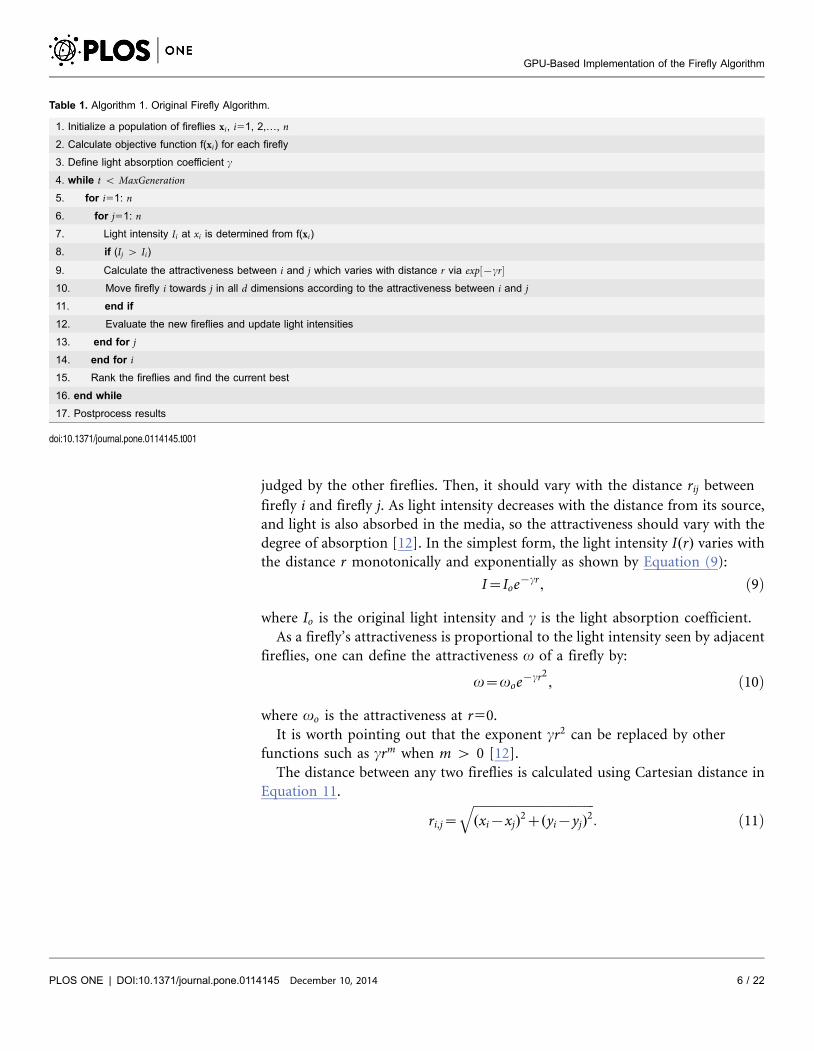
with other fireflies, especially to prey attraction [16]. Algorithm 1 (Table 1) shows

a pseudocode for the original FA.

In the Algorithm 1 (Table 1), there are two important issues: the variation of

light intensity and the attractiveness formulation. For simplicity, one can assume

that the attractiveness of a firefly is determined by its brightness or light intensity

which is associated with the encoded objective function [10]. The brightness I of a

firefly at a particular location x can be chosen as I(x) [ f (x). However, the

attractiveness v is relative, which should be seen in the eyes of the beholder or



judged by the other fireflies. Then, it should vary with the distance rij between

firefly i and firefly j. As light intensity decreases with the distance from its source,

and light is also absorbed in the media, so the attractiveness should vary with the

degree of absorption [12]. In the simplest form, the light intensity I(r) varies with

the distance r monotonically and exponentially as shown by Equation (9):

I~Ioe{cr, ð9Þ

where Io is the original light intensity and c is the light absorption coefficient.

As a firefly’s attractiveness is proportional to the light intensity seen by adjacent

fireflies, one can define the attractiveness v of a firefly by:

v~voe{cr2, ð10Þ

where vo is the attractiveness at r50.

It is worth pointing out that the exponent cr2 can be replaced by other

functions such as crm when m w 0 [12].

The distance between any two fireflies is calculated using Cartesian distance in

Equation 11.

ri,j~

ffiffiffiffiffiffiffiffiffiffiffiffiffiffiffiffiffiffiffiffiffiffiffiffiffiffiffiffiffiffiffiffiffiffiffiffiffiffi(xi{xj)

2z(yi{yj)2

q: ð11Þ

Table 1. Algorithm 1. Original Firefly Algorithm.

1. Initialize a population of fireflies xi, i51, 2,…, n

2. Calculate objective function f(xi) for each firefly

3. Define light absorption coefficient c

4. while t v MaxGeneration

5. for i51: n

6. for j51: n

7. Light intensity Ii at xi is determined from f(xi)

8. if (Ij w Ii)

9. Calculate the attractiveness between i and j which varies with distance r via exp½{cr�10. Move firefly i towards j in all d dimensions according to the attractiveness between i and j

11. end if

12. Evaluate the new fireflies and update light intensities

13. end for j

14. end for i

15. Rank the fireflies and find the current best

16. end while

17. Postprocess results

doi:10.1371/journal.pone.0114145.t001



The firefly i is attracted to brighter firefly j and its movement is determined by

xi~xjzv0e{cr2

i,j(xj{xi)za(rand{12

): ð12Þ

In Equation (12), xi is the current position or solution of a firefly and the

v0e{cr2i,j(xj{xi) is attractiveness of a firefly to seen by adjacent fireflies. The

a(rand{ 12 ) is a firefly’s random movement. The coefficient a is a randomisation

parameter determined by the problem of interest with a [ [0,1], while rand

function is a random number obtained from the uniform distribution. Without

the random movement, the reies would possibly be attracted to a rey that is not

necessarily the brightest. The solution would be restricted to a local minima,

directly toward the best solution in the local search space. Using the

randomization term, the search over small deviations makes it possible to escape

from local minima, having a higher chance of nding the global minimum of the

function.

For most cases related in others works, they take v0~1, a [ [0,1] and c~1. The

parameter c characterizes the variation of attractiveness, and its value is crucially

important in determining the speed of the convergence and how the FA algorithm

behaves. In most applications, it typically varies from 0:01 to 100.

According with Yang [38], the algorithm is swarm-intelligence-based, so it has

the similar advantages that other swarm-intelligence-based algorithms have. In

fact, a simple analysis of parameters suggest that some particle swarm

optimization (PSO) variants such as Accelerated PSO are a special case of firefly

algorithm when c~0. However, according with Yang [38], firefly has two major

advantages over other algorithms: automatical subdivision and the ability of

dealing with multimodality. First, FA is based on attraction and atractiveness

decrease with distance. This leads to the fact that the whole population can

automatically subdivide into subgroups, and each group can swarm around each

mode or local optimum. Second, this subdivision allows the fireflies to be able to

find all optima simultaneously if the population size is sufficiently higher than the

number of modes.

The Proposed Multiobjective FA for Variable Selection

Based on the success of the works cited in ‘‘Introdution’’, one found out that FA

can be used for selection of variables to solve multivariate calibration problems.

Thus, this paper presents a FA for variable selection using MLR (FA-MLR).

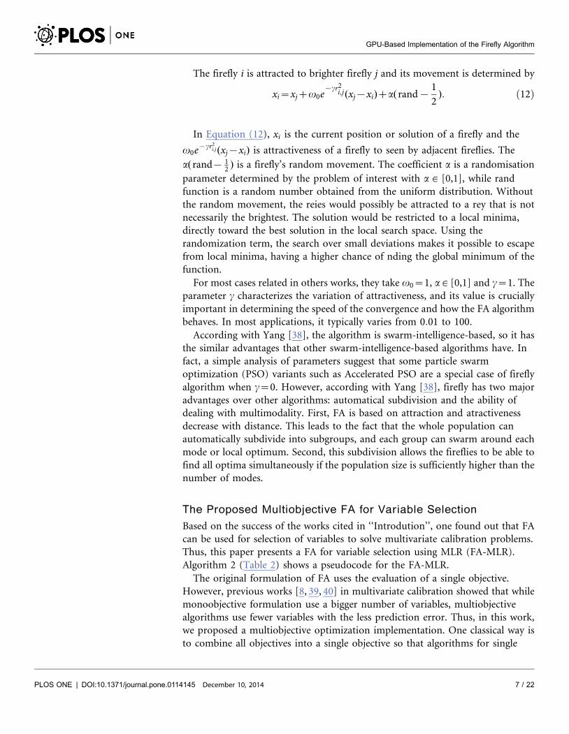
Algorithm 2 (Table 2) shows a pseudocode for the FA-MLR.

The original formulation of FA uses the evaluation of a single objective.

However, previous works [8, 39, 40] in multivariate calibration showed that while

monoobjective formulation use a bigger number of variables, multiobjective

algorithms use fewer variables with the less prediction error. Thus, in this work,

we proposed a multiobjective optimization implementation. One classical way is

to combine all objectives into a single objective so that algorithms for single



objective optimization. Another way is to extend the firefly algorithm to produce

Pareto optimal front directly. By extending the basic formulation of FA, we

developed the following multiobjective firefly algorithm, based on [41],

summarized in Algorithm 2 (Table 2).

In the multiobjective formulation of FA, the choice of current best is done in

two steps. First, only the non-dominated solutions are selected. In mathematical

terms, a feasible solution x1[X is said dominate another solution x2[X if:

1. fi(x1)ƒfi(x2) for all indices i [ f1,2, . . . ,kg and

2. fj(x1)ƒfj(x2) for at least one index j [ f1,2, . . . ,kgA solution x1[X is called Pareto optimal, if there does not exist another

solution that dominates it. Among non-dominates solutions, we applied the

multiobjective decision maker method described in [8] to choice the current best

(step 10).

Numerical Example

For illustration, let’s consider a short variable selection problem with just five

variables available and just three fireflies. Will be used, the first five variables

available and the first three samples from matrix X and the first three samples

from vector y described in Materials and Methods Section, using a~0:2, c~1and v0~0:97. First, the fireflies are uniformly distributed random numbers in the

range 0 to 1.

Firefly 1 5 0.95 0.48 0.45 0.44 0.92,

Firefly 2 5 0.23 0.89 0.01 0.61 0.73,

Firefly 3 5 0.60 0.76 0.82 0.79 0.17.

The variable selection is a binary problem, so each firefly must be encoded.

Each variable information major than 0.5 is encoded to 1 (variable will be used in

Table 2. Algorithm 2. Proposed FA-MLR.

1. Parameters: Xn|m, yn|1, where Xn|m is a matrix of samples by their corresponding variable values, n is the number of rows, m is the number of columnsand yn|1 is a vector of dependent variables

2. s / the number of fireflies, determined by experimental analysis.

3. for i51: MaxGeneration

4. Generate randomly a population of s fireflies, where each firefly is a set of d indices for d columns of Xn|m, d ƒ m

5. Compute Equation (2) for each firefly (when using Algorithm 3 it is performed on the GPU)

6. Compute the number of variables used in the model

7. Calculate Equation (3) determining the light intensities of each firefly

8. If i-th firefly dominates j-th firefly

9. Move firefly j towards i using Equation (12)

10. Rank the fireflies and find the current best

11. end for i

12. Postprocess results, that is, calculate the prediction error for the best firefly and visualize the selected variables indicated by it.




the regression model) and less or equal 0.5 is encoded 0 (variable will not be used

in the regression model).

Encoded Firefly 1 5 1 0 0 0 1,

Encoded Firefly 2 5 0 1 0 1 1,

Encoded Firefly 3 5 1 1 1 1 0.

Now, each firefly will be evaluated using the Equation 2. This equation indicates

the error of prediction. In Equation 2, just the columns of X indicated by firefly

will be used in the regression. In our example the brightness is 6.82 10.97 9.22for

each firefly. Now, we compared all firefly each other, for example, the firefly 2 has

major light intensity than firefly 1, so we must move firefly 1 toward firefly 2. For

this proposes, first we must calculate the distance between the fireflies using

Equation 11.

r1,2 5 0.71 0.40 0.43 0.17 0.18

Using the distance between the fireflies, we can calculate the attractiveness using

Equation 10. As a result, we updated firefly 1 and the encoded firefly 1. Worth

noting that, the updated firefly 1 excluded the first variable used in the original

solution and now use the second and fourth variables available after ‘to walk’

toward firefly 2.

Updated Firefly 1 5 0.44 0.75 0.02 0.53 0.67?Updated Encoded Firefly 1 5 0 1 0 1 1

The iteration is repeated until all solutions have been updated. The updates

allow the solutions to move towards to the current optimal solution. The solution

that produces the best fitness (in this case the minor RMSEP value) is selected as

the global best solution.

Using a GPU with the CUDA-MATLAB integration for the FA-MLR

GPUs are microprocessors developed with a flow-oriented technology, optimized

for calculations of data-intensive, where many identical operations can be

performed in parallel on different data [42]. Graphics devices currently available

represent a high performance computer hardware, flexible by enabling the

execution of non-graphical applications [5]. While the current multicore

architectures have two, four or eight cores, GPUs have hundreds or even

thousands of processing cores [5]. GPUs can implement many parallel algorithms

directly using graphics hardware and the current trend is to include in each new

generation a significant number of additional cores [43].

Correspondingly the evolution of hardware, new programming models have

been developed. Among them stand out Compute Unified Device Architecture

(CUDA) [42] and Open Computing Language (OpenCL) [44]. In both, due to the

availability of Application Programming Interface (API) to the programmer the

implementation of efficient parallel applications is facilitated [5]. CUDA was the

first architecture and programming interface, created by NVIDIA in 2006 to allow

GPUs could be used for a wide variety of applications [42].

Recently, using MATLAB for GPU computing can accelerate the applications

more easily than by using the CUDA-C programming language [45]. This is



possible because of the existence of MATLAB plug-in for CUDA (Parallel

Computing Toolbox - PCT). Thus, with the familiar MATLAB language one can

take advantage of the CUDA GPU computing technology [46].

Developments for GPUs using the PCT is in general easier and faster than using

CUDA-C language, since several aspects of parallelization design are performed by

the PCT [47, 48]. Furthermore, it is important to note that the PCT requires an

NVIDIA graphics card.

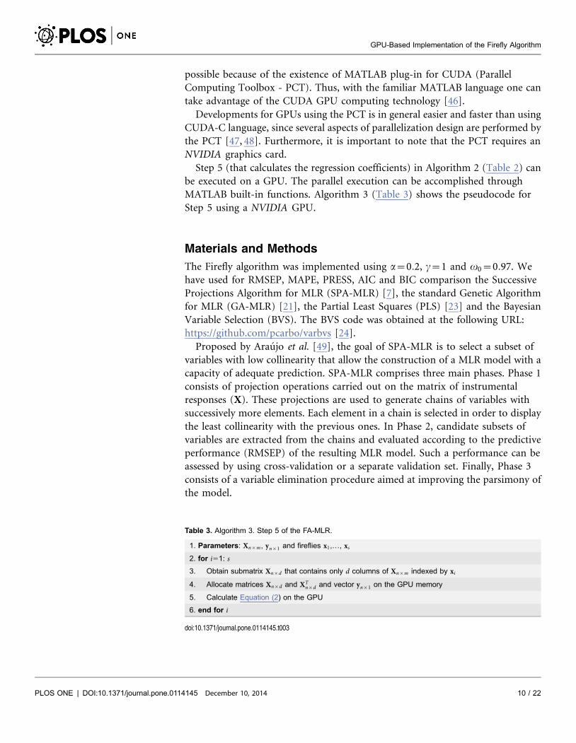
Step 5 (that calculates the regression coefficients) in Algorithm 2 (Table 2) can

be executed on a GPU. The parallel execution can be accomplished through

MATLAB built-in functions. Algorithm 3 (Table 3) shows the pseudocode for

Step 5 using a NVIDIA GPU.

Materials and Methods

The Firefly algorithm was implemented using a~0:2, c~1 and v0~0:97. We

have used for RMSEP, MAPE, PRESS, AIC and BIC comparison the Successive

Projections Algorithm for MLR (SPA-MLR) [7], the standard Genetic Algorithm

for MLR (GA-MLR) [21], the Partial Least Squares (PLS) [23] and the Bayesian

Variable Selection (BVS). The BVS code was obtained at the following URL:

https://github.com/pcarbo/varbvs [24].

Proposed by Araujo et al. [49], the goal of SPA-MLR is to select a subset of

variables with low collinearity that allow the construction of a MLR model with a

capacity of adequate prediction. SPA-MLR comprises three main phases. Phase 1

consists of projection operations carried out on the matrix of instrumental

responses (X). These projections are used to generate chains of variables with

successively more elements. Each element in a chain is selected in order to display

the least collinearity with the previous ones. In Phase 2, candidate subsets of

variables are extracted from the chains and evaluated according to the predictive

performance (RMSEP) of the resulting MLR model. Such a performance can be

assessed by using cross-validation or a separate validation set. Finally, Phase 3

consists of a variable elimination procedure aimed at improving the parsimony of

the model.

Table 3. Algorithm 3. Step 5 of the FA-MLR.

1. Parameters: Xn|m, yn|1 and fireflies x1,…, xs

2. for i51: s

3. Obtain submatrix Xn|d that contains only d columns of Xn|m indexed by xi

4. Allocate matrices Xn|d and XTn|d and vector yn|1 on the GPU memory

5. Calculate Equation (2) on the GPU

6. end for i




In GA-MLR, the RMSEP guide the evaluation of a subset of variables used in

the calibration model and allows us to choose models more suitable to prediction

[21]. Genetic algorithms (GA) are a global search heuristic inspired on the natural

evolution of species and in the natural biological process. Basically, a GA creates a

population of possible solutions to the problem being solved and then submit

these solutions to the evolution process. Genetic operators are applied to

transform the population in every generation, in order to created better

individuals. The main operators responsible for the population diversification well

known in the literature are crossover (or recombination) and mutation.

Partial Least Squares (PLS) is a technique that generalizes and combines

features from principal component analysis and MLR [30]. It is a statistical

method that bears some relation to principal components regression. Instead of

finding hyperplanes of minimum variance between the response and independent

variables, it finds a linear regression model by projecting the predicted variables

and the observable variables to a new space. Because both the X and y data are

projected to new spaces, the PLS family of methods are known as bilinear factor

models.

Bayesian Variable Selection (BVS) is a tool to variable selection in MLR used for

tackling many scientific problems [24]. In the BVS, the model selection problem is

transformed to the form of parameter estimation: rather than searching for the

single optimal model, a Bayesian will attempt to estimate the posterior probability

of all models within the considered class of models. A probability distribution is

first assigned to the dependent variable through the specification of a family of

prior distributions for the unknown parameters in the regression model. For each

regression coefficient subject to deletion from the model, the prior distribution is

a mixture of a point mass at 0 and diffuse uniform distribution elsewhere.

The Kennard and Stone [50] algorithm was applied to the resulting spectra to

divide the samples into calibration, validation and prediction sets with 389, 193

and 193 samples, respectively. The validation set was employed to guide the

selection of variables in SPA-MLR and GA-MLR. The prediction set was only

employed in the final performance assessment of the resulting MLR models. In the

PLS study, the calibration and validation sets were joined into a single modeling

set, which was used in the leave-one-out cross-validation procedure. The number

of latent variables was selected on the basis of the cross-validation error by using

the F-test criterion of Haaland and Thomas [23]. The prediction set was only

employed in the final evaluation of the PLS model.

All calculations were carried out by using a desktop computer with an Intel

Core i7 2600 (3.40 GHz), 8 GB of RAM memory and a NVIDIA GeForce GTX

550Ti graphics card with 192 CUDA cores and 2 GB of memory config. The

Matlab 8.1.0.604 (R2013a) software platform was employed throughout.

We present two studies, one simulated and a real problem, to present the

proposed algorithm. The details of the data sets are presented below.



Simulated Data Set

The simulated data set used in this work was generated using the matlab code

showed by S1 Source Code. The algorithm uses a random numbers generation for

building the matrix X (independents variables). The seed of the random generator

was setted with value 0 (zero), thus, the experiment can be reproduced in any

computer. To generate the matrix responses Y, we choose a number of variables

from X to be correlated with Y (dependents variables). The values of Y are

generated using random weights applied over the variables chosen. We create two

scenarios: the first five variables are randomly chosen to be correlated with Y and

in the second, ten variables are used. The challenge of variable selection algorithm

is to find the variables used to generate Y. These variables explain the Y variability

and the best result can be obtained selecting only these variables.

Real Data Set

The real dataset employed in this work consists of whole grain wheat samples,

obtained from vegetal material from occidental Canadian producers. The standard

data were determined at the Grain Research Laboratory as in work of [7], [5] and

[51]. The data set for the multivariate calibration study consists of 1090 Near-

Infrared (NIR) spectra of whole-kernel wheat samples, which were used as shoot-

out data in the 2008 International Diffuse Reflectance Conference (http://www.

idrc-chambersburg.org/shootout.html).

Protein content was chosen as the property of interest (matrix Y). The spectra

were acquired in the range 400–2500 nm with a resolution of 2 nm (matrix X). In

this work the NIR region in the range 1100–2500 nm was employed. In order to

remove undesirable baseline features, first derivative spectra were calculated by

using a Savitzky-Golay filter with a 2nd order polynomial and an 11-points

window [52].

The reference values of protein concentration in samples of wheat were

determined in the laboratory by the Kjeldahl method [53]. This method uses the

destruction of organic matter with concentrated sulfuric acid in the presence of a

catalyst and by the action of heat, with subsequent distillation and titration of

nitrogen from the sample. The use of indirect instrumental methods such as NIR

spectroscopy and mathematical models such as MLR allow the protein to be

determined without destruction of the sample.

Results and Discussion

Simulated Study

In the simulated study, the challenge of the variable selection algorithms is to find

the variables in X that explain the Y variance. We did two studies, one with five

variables generating Y, and other with ten variables generating Y.

Table 4 presents the results of all algorithms in the simulated data. As can be

seen, the FA-MLR has the minor value of RMSEP, MAPE and PRESS, in both



http://www.idrc-chambersburg.org/shootout.html

http://www.idrc-chambersburg.org/shootout.html

studies, using five and ten variables generating Y. This measures indicates better

prediction ability using the variables selected by FA. FA-MLR use less variables

than SPA-MLR and BVS. According with AIC and BIC measure, FA-MLR has

better parsimony between predictive capacity and number of variables in the

model. In some applications the predictive ability is critical, in others the number

of variables used or even the parsimony between both.

Table 5 shows the variable selected by each one of the algorithms. For the first

case, the variables used to generating Y is 22, 32, 34, 40 and 99. For the second

case, the variables used were 4, 11, 39, 46, 48, 66, 67, 69, 85 and 189. According

with results, for the two cases SPA-MLR and FA-MLR are the more conservative

algorithm. SPA-MLR selected just two variables (32 and 99) for the first case, but

did not select the other three variables correlated with the response matrix Y. FA-

MLR selected three variables (22, 32 and 40), all correlated whit the response

matrix Y, generating a prediction error lower than SPA-MLR. In the second case,

SPA-MLR selected three variables (11, 39 and 85) correlated with the response

and one wrong variable. FA-MLR selected three variables (4, 46 and 189) all of

them related with the response variable. Although the SPA-MLR algorithm use a

elimination procedure, described in [54], the multiobjective formulation of FA-

MLR was able to balance between prediction error and number of variables. The

results of AIC and BIC show that FA-MLR algorithm has better parsimony of

MLR models than models builded by SPA-MLR.

The best result of RMPSEP, MAPE and PRESS were obtained by FA-MLR in

both cases. The algorithm selected more variables correlated with the response

matrix (3 in both cases) reducing the prediction error. FA-MLR works

individually each firefly and finds a better position for itself in consideration with

its current position as well as the position of other fireflies. Thus, it escapes from

the local optima and finds a global optimum is less number of iterations.

Table 4. Results of the FA-MLR, SPA-MLR, GA-MLR, PLS and BVS, in simulated data.

Number of Variables RMSEP MAPE AIC BIC PRESS

Five variables generating Y

PLS 4 1.11 3.7% 1279 1330 29.29

SPA-MLR 2 1.05 3.53% 1005 1020 26.82

GA-MLR 26 1.85 4.0% 1981 2013 45.42

BVS 4 0.98 3.4% 1201 1301 21.02

FA-MLR 3 0.97 3.3% 956 972 19.98

Ten variables generating Y

PLS 4 1.91 3.5% 1054 1093 69.05

SPA-MLR 4 1.75 3.2% 1004 1021 61.26

GA-MLR 35 2.01 4.80% 1791 1807 74.36

BVS 7 1.95 3.3% 1149 1201 70.95

FA-MLR 3 1.67 3.1% 901 933 57.5




However, the algorithm requires a correct adjustment of the parameters, while

SPA-MLR, PLS and BVS not.

The worst result was obtained by GA-MLR algorithm. It selected much wrong

variables and few variables correlated with the response matrix. The model

produce by this algorithm is large and with low prediction ability. PLS uses linear

transformation of original variables to build new latent variables. In this process is

not possible separate the original variables used, thus, we do not have the results

of which original variables used to build the regression model.

Real Problem

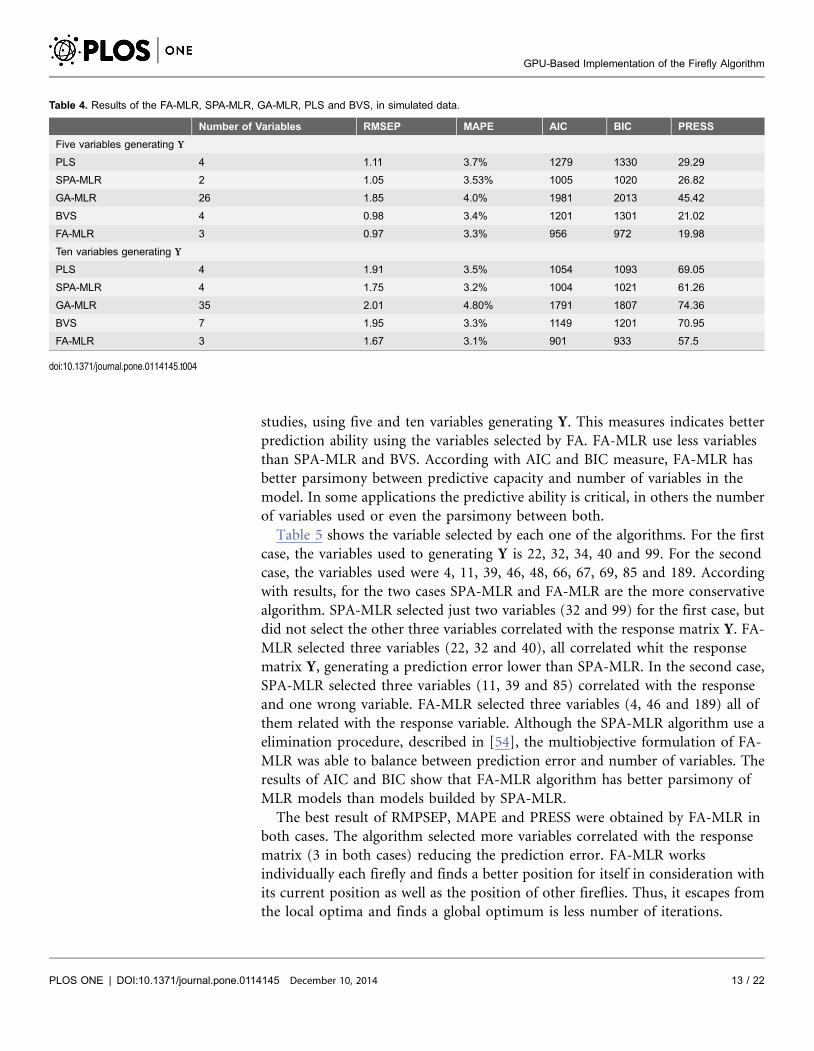
Fig. 1 shows that the FA-MLR is able to perform the reduction of the RMSEP as

the iterations are performed. The curve in the graph refers to the average error of

all the fireflies.

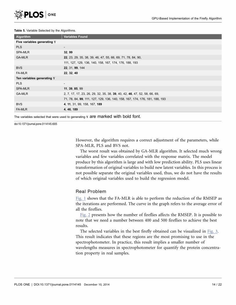
Fig. 2 presents how the number of fireflies affects the RMSEP. It is possible to

note that we need a number between 400 and 500 fireflies to achieve the best

results.

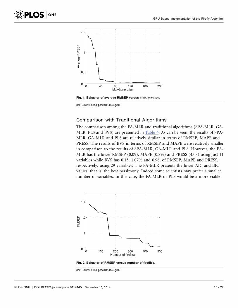
The selected variables in the best firefly obtained can be visualized in Fig. 3.

This result indicates that these regions are the most promising to use in the

spectrophotometer. In practice, this result implies a smaller number of

wavelengths measures in spectrophotometer for quantify the protein concentra-

tion property in real samples.

Table 5. Variable Selected by the Algorithms.

Algorithm Variables Found

Five variables generating Y

PLS -

SPA-MLR 32, 99

GA-MLR 22, 23, 29, 35, 38, 39, 46, 47, 55, 66, 69, 71, 78, 84, 90,

111, 127, 129, 136, 140, 158, 167, 174, 176, 188, 193

BVS 22, 31, 99, 144

FA-MLR 22, 32, 40

Ten variables generating Y

PLS -

SPA-MLR 11, 39, 85, 99

GA-MLR 2, 7, 17, 17, 23, 26, 29, 32, 35, 38, 39, 40, 42, 46, 47, 52, 58, 66, 69,

71, 78, 84, 99, 111, 127, 129, 136, 140, 158, 167, 174, 176, 181, 188, 193

BVS 4, 11, 31, 99, 158, 167, 189

FA-MLR 4, 46, 189

The variables selected that were used to generating Y are marked with bold font.




Comparison with Traditional Algorithms

The comparison among the FA-MLR and traditional algorithms (SPA-MLR, GA-

MLR, PLS and BVS) are presented in Table 6. As can be seen, the results of SPA-

MLR, GA-MLR and PLS are relatively similar in terms of RMSEP, MAPE and

PRESS. The results of BVS in terms of RMSEP and MAPE were relatively smaller

in comparison to the results of SPA-MLR, GA-MLR and PLS. However, the FA-

MLR has the lower RMSEP (0.09), MAPE (0.8%) and PRESS (4.08) using just 11

variables while BVS has 0.15, 1.07% and 6.96, of RMSEP, MAPE and PRESS,

respectively, using 29 variables. The FA-MLR presents the lower AIC and BIC

values, that is, the best parsimony. Indeed some scientists may prefer a smaller

number of variables. In this case, the FA-MLR or PLS would be a more viable

Fig. 1. Behavior of average RMSEP versus MaxGeneration.

doi:10.1371/journal.pone.0114145.g001

Fig. 2. Behavior of RMSEP versus number of fireflies.




choice. However, despite to select a relatively small number of variables PLS uses

all the original variables to build the new latent variables [55].

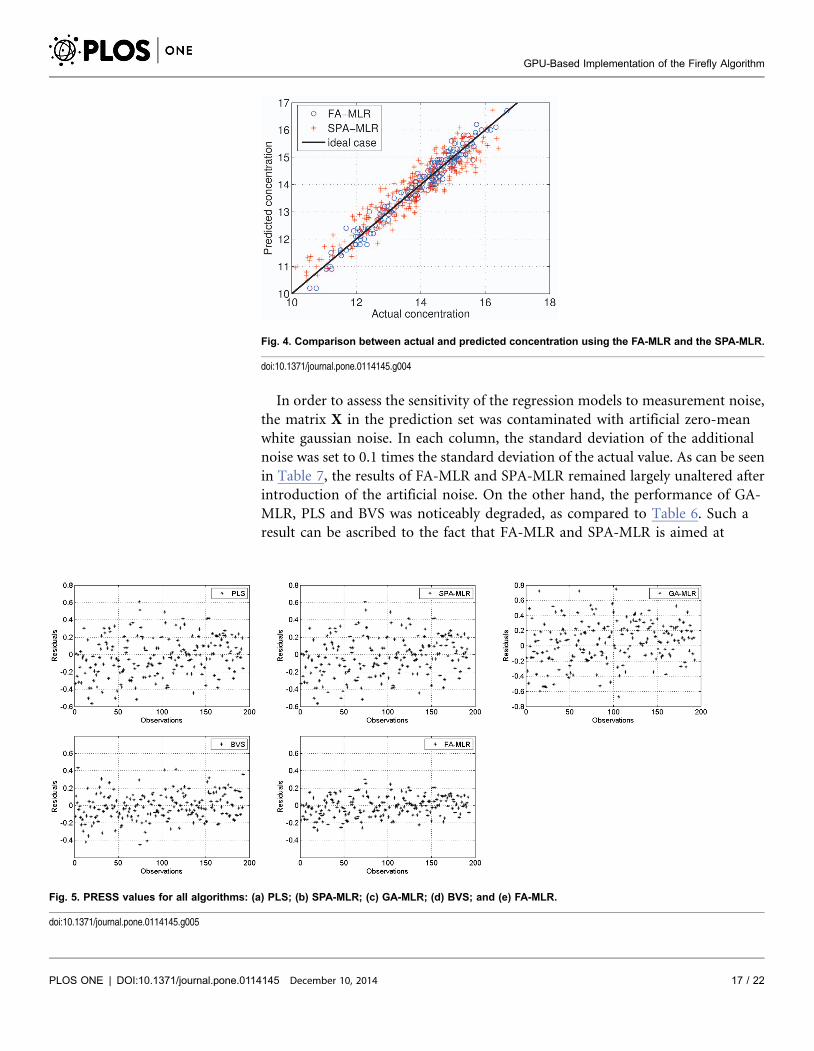
Fig. 4 plots the real values in the compound versus predictions using the SPA-

MLR (red plus) and FA-MLR (blue balls), that produced the best performance

among the rival-tested algorithms. Zero differences between predictions and

actual concentrations result in points over the straight line of the plot. The

predicted concentrations are near the real concentrations for both methods.

Nevertheless, the model using the variables selected by FA-MLR are in general

closer to the straight line than SPA-MLR predictions. This result also indicates

that the MLR model obtained using the variables selected by FA-MLR can

produce less RMSEP and MAPE in average.

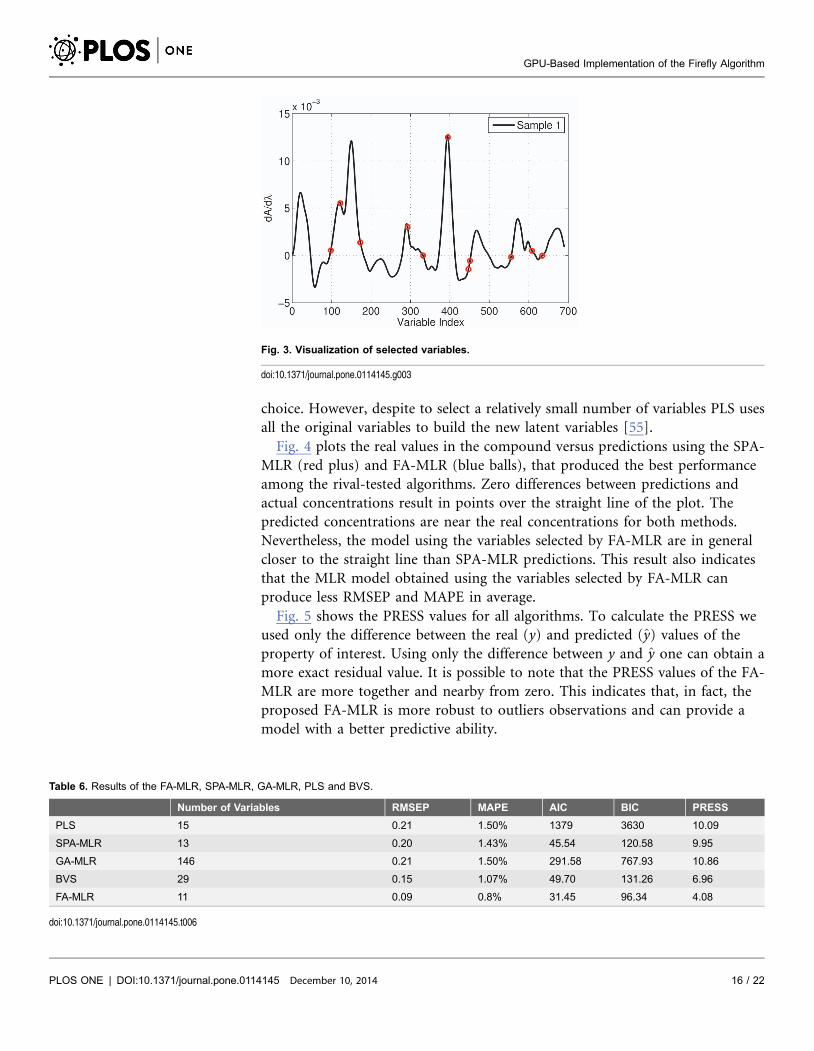
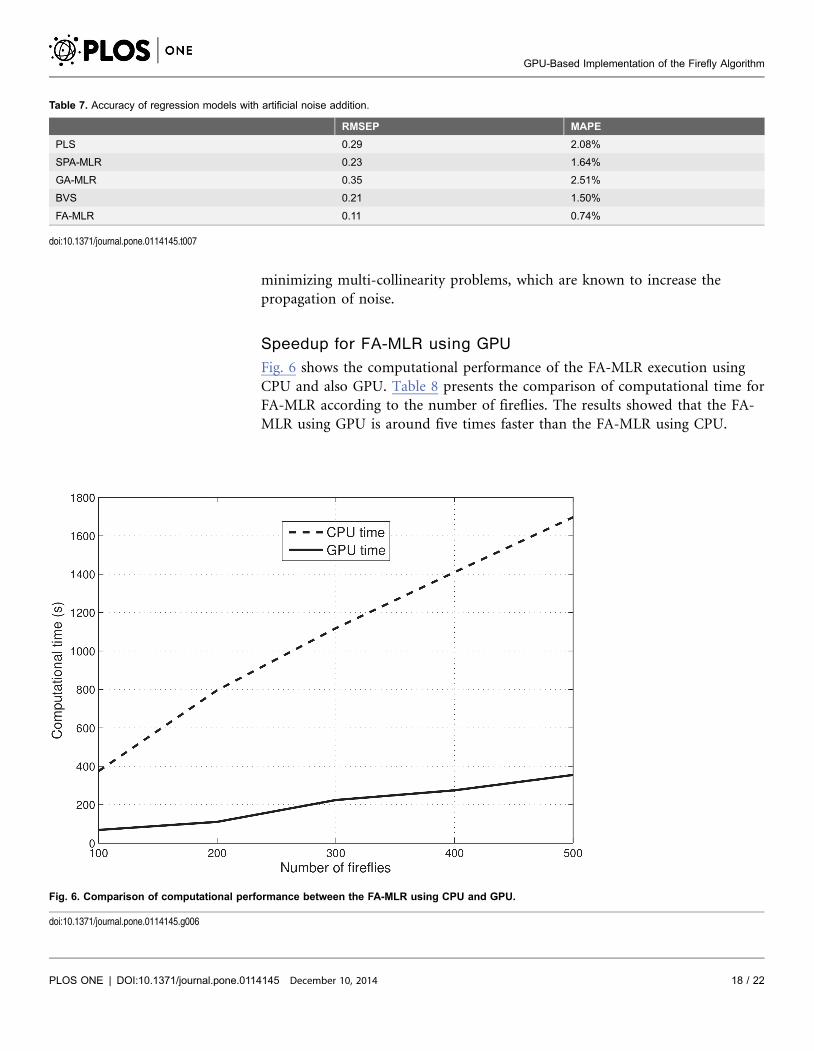
Fig. 5 shows the PRESS values for all algorithms. To calculate the PRESS we

used only the difference between the real (y) and predicted (y) values of the

property of interest. Using only the difference between y and y one can obtain a

more exact residual value. It is possible to note that the PRESS values of the FA-

MLR are more together and nearby from zero. This indicates that, in fact, the

proposed FA-MLR is more robust to outliers observations and can provide a

model with a better predictive ability.

Fig. 3. Visualization of selected variables.


Table 6. Results of the FA-MLR, SPA-MLR, GA-MLR, PLS and BVS.

Number of Variables RMSEP MAPE AIC BIC PRESS

PLS 15 0.21 1.50% 1379 3630 10.09

SPA-MLR 13 0.20 1.43% 45.54 120.58 9.95

GA-MLR 146 0.21 1.50% 291.58 767.93 10.86

BVS 29 0.15 1.07% 49.70 131.26 6.96

FA-MLR 11 0.09 0.8% 31.45 96.34 4.08




In order to assess the sensitivity of the regression models to measurement noise,

the matrix X in the prediction set was contaminated with artificial zero-mean

white gaussian noise. In each column, the standard deviation of the additional

noise was set to 0.1 times the standard deviation of the actual value. As can be seen

in Table 7, the results of FA-MLR and SPA-MLR remained largely unaltered after

introduction of the artificial noise. On the other hand, the performance of GA-

MLR, PLS and BVS was noticeably degraded, as compared to Table 6. Such a

result can be ascribed to the fact that FA-MLR and SPA-MLR is aimed at

Fig. 4. Comparison between actual and predicted concentration using the FA-MLR and the SPA-MLR.


Fig. 5. PRESS values for all algorithms: (a) PLS; (b) SPA-MLR; (c) GA-MLR; (d) BVS; and (e) FA-MLR.




minimizing multi-collinearity problems, which are known to increase the

propagation of noise.

Speedup for FA-MLR using GPU

Fig. 6 shows the computational performance of the FA-MLR execution using

CPU and also GPU. Table 8 presents the comparison of computational time for

FA-MLR according to the number of fireflies. The results showed that the FA-

MLR using GPU is around five times faster than the FA-MLR using CPU.

Table 7. Accuracy of regression models with artificial noise addition.

RMSEP MAPE

PLS 0.29 2.08%

SPA-MLR 0.23 1.64%

GA-MLR 0.35 2.51%

BVS 0.21 1.50%

FA-MLR 0.11 0.74%


Fig. 6. Comparison of computational performance between the FA-MLR using CPU and GPU.




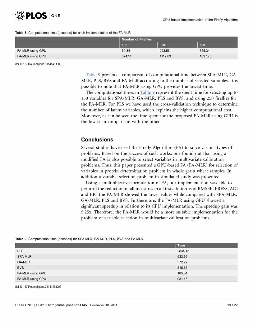
Table 9 presents a comparison of computational time between SPA-MLR, GA-

MLR, PLS, BVS and FA-MLR according to the number of selected variables. It is

possible to note that FA-MLR using GPU provides the lowest time.

The computational times in Table 9 represent the spent time for selecting up to

150 variables for SPA-MLR, GA-MLR, PLS and BVS, and using 250 fireflies for

the FA-MLR. For PLS we have used the cross-validation technique to determine

the number of latent variables, which explains the higher computational cost.

Moreover, as can be seen the time spent for the proposed FA-MLR using GPU is

the lowest in comparison with the others.

Conclusions

Several studies have used the Firefly Algorithm (FA) to solve various types of

problems. Based on the success of such works, one found out that using a

modified FA is also possible to select variables in multivariate calibration

problems. Thus, this paper presented a GPU-based FA (FA-MLR) for selection of

variables in protein determination problem in whole grain wheat samples. In

addition a variable selection problem in simulated study was presented.

Using a multiobjective formulation of FA, our implementation was able to

perform the reduction of all measures in all tests. In terms of RMSEP, PRESS, AIC

and BIC the FA-MLR showed the lower values while compared with SPA-MLR,

GA-MLR, PLS and BVS. Furthermore, the FA-MLR using GPU showed a

significant speedup in relation to its CPU implementation. The speedup gain was

5.25x. Therefore, the FA-MLR would be a more suitable implementation for the

problem of variable selection in multivariate calibration problems.

Table 8. Computational time (seconds) for each implementation of the FA-MLR.

Number of Fireflies

100 300 500

FA-MLR using GPU 69.34 223.56 355.34

FA-MLR using CPU 374.51 1119.63 1697.78


Table 9. Computational time (seconds) for SPA-MLR, GA-MLR, PLS, BVS and FA-MLR.

Time

PLS 2834.15

SPA-MLR 533.66

GA-MLR 372.22

BVS 315.68

FA-MLR using GPU 185.34

FA-MLR using CPU 931.45




In future works, larger multivariate calibration problems may be solved. In

addition, alternatives to CUDA-MATLAB integration such as OpenCL could be

investigated for comparative studies.

Supporting Information

S1. Source Code

doi:10.1371/journal.pone.0114145.s001 (DOCX)

Author Contributions

Conceived and designed the experiments: LCMP ASS TWL. Performed the

experiments: LCMP ASS. Analyzed the data: LCMP ASS TWL ACBD CJC ARGF.

Contributed reagents/materials/analysis tools: LCMP ASS TWL ACBD CJC

ARGF. Wrote the paper: LCMP ASS.

References

1. Brown SD, Blank TB, Sum ST, Weyer LG (1994) Chemometrics. Analytical chemistry 66: 315–359.

2. Ferreira MMC, Antunes AM, Melgo MS, Volpe PLO (1999) Quimiometria I: calibracao multivariada, umtutorial. Quimica Nova 22: 724–731.

3. George EI (2000) The variable selection problem. Journal of the American Statistical Association 95:1304–1308.

4. Coifman RR, Wickerhauser MV (1992) Entropy-based algorithms for best basis selection. InformationTheory, IEEE Transactions on 38: 713–718.

5. Paula LCM, Soares AS, Lima TW, Martins WS, Filho ARG, et al. (2013) Partial parallelization of thesuccessive projections algorithm using compute unified device architecture. In: Internation Conferenceon Parallel and Distributed Processing Techniques and Applications. pp.737–741.

6. Chau FT, Liang YZ, Gao J, Shao XG (2004) Chemometrics: from basics to wavelet transform, volume234. Wiley. com.

7. Galvao Filho AR, Galvao RK, Araujo MCU (2011) Effect of the subsampling ratio in the application ofsubagging for multivariate calibration with the successive projections algorithm. Journal of the BrazilianChemical Society 22: 2225–2233.

8. Lucena DV, Lima TW, Soares AS, Delbem ACB, Galvao AR, et al. (2013) Multi-objective evolutionaryalgorithm for variable selection in calibration problems: A case study for protein concentration prediction.In: Proceedings of 2013 IEEE Congress on Evolutionary Computation. pp.1053–1059.

9. Yang XS (2008) Nature-inspired metaheuristic algorithms. Luniver Press.

10. Yang XS (2009) Firefly algorithms for multimodal optimization. In: Stochastic algorithms: foundationsand applications, Springer. pp.169–178.

11. Lukasik S, Zak S (2009) Firefly algorithm for continuous constrained optimization tasks. In:Computational Collective Intelligence. Semantic Web, Social Networks and Multiagent Systems,Springer. pp.97–106.

12. Yang XS (2010) Firefly algorithm, stochastic test functions and design optimisation. International Journalof Bio-Inspired Computation 2: 78–84.

13. Senthilnath J, Omkar S, Mani V (2011) Clustering using firefly algorithm: Performance study. Swarmand Evolutionary Computation 1: 164–171.



http://www.plosone.org/article/fetchSingleRepresentation.action?uri=info:doi/10.1371/journal.pone.0114145.s001

14. Gandomi AH, Yang XS, Alavi AH (2011) Mixed variable structural optimization using firefly algorithm.Computers & Structures 89: 2325–2336.

15. Jati GK, Suyanto (2011) Evolutionary discrete firefly algorithm for travelling salesman problem. In:Adaptive and Intelligent Systems, Springer. pp.393–403.

16. Banati H, Bajaj M (2011) Fire fly based feature selection approach. International Journal of ComputerScience Issues 8: 473–480.

17. Horng MH (2012) Vector quantization using the firefly algorithm for image compression. Expert Systemswith Applications 39: 1078–1091.

18. Abdullah A, Deris S, Anwar S, Arjunan SN (2013) An evolutionary firefly algorithm for the estimation ofnonlinear biological model parameters. PloS one 8: e56310.

19. Husselmann AV, Hawick K (2012) Parallel parametric optimisation with firefly algorithms on graphicalprocessing units. In: Proc. Int. Conf. on Genetic and Evolutionary Methods (GEM12). Number CSTN-141, Las Vegas, USA, CSREA (16–19 July 2012). pp.77–83.

20. Husselmann A, Hawick K (2014) Geometric firefly algorithms on graphical processing units. In: CuckooSearch and Firefly Algorithm, volume 516. pp.245–269.

21. Soares AS, Delbem ACB, Lima TW, Coelho CJ, Soares FAAMN (2013) Mutation-based compactgenetic algorithm for spectroscopy variable selection in the determination of protein in wheat grainsamples. Eletronic Letters 49: 80–92.

22. Soares AS, de Lima TW, Soares FAAMN, Coelho CJ, Federson FM, et al. (2014) Mutation-basedcompact genetic algorithm for spectroscopy variable selection in determining protein concentration inwheat grain. Electronics Letters 50: 932–934(2).

23. Haaland DM, Thomas EV (1988) Partial least-squares methods for spectral analyses. 1. relation toother quantitative calibration methods and the extraction of qualitative information. Analytical Chemistry60: 1193–1202.

24. Carbonetto P, Stephens M (2012) Scalable variational inference for bayesian variable selection inregression, and its accuracy in genetic association studies. Bayesian Analysis 7: 73–108.

25. Martens H (1991) Multivariate calibration. John Wiley & Sons.

26. Westad F, Martens H (2000) Variable selection in near infrared spectroscopy based on significancetesting in partial least squares regression. Journal of Near Infrared Spectrosc 8: 117–124.

27. Naes T, Mevik BH (2001) Understanding the collinearity problem in regression and discriminantanalysis. Journal of Chemometrics 15: 413–426.

28. Cortina JM (1994) Interaction, nonlinearity, and multicollinearity: Implications for multiple regression.Journal of Management 19: 915–922.

29. Beebe KR, Pell RJ, Seasholtz MB (1998) Chemometrics: a practical guide. Wiley-Interscience Serieson Laboratory Automation, 341 pp.

30. Lawson CL, Hanson RJ (1974) Solving least squares problems, volume 161. SIAM.

31. Hibon M, Makridakis S (1995) Evaluating accuracy (or error) measures. INSEAD.

32. Allen DM (1974) The relationship between variable selection and data agumentation and a method forprediction. Technometrics 16: 125–127.

33. Tarpey T (2000) A note on the prediction sum of squares statistic for restricted least squares. TheAmerican Statistician 54: 116–118.

34. Bartoli A (2009) On computing the prediction sum of squares statistic in linear least squares problemswith multiple parameter or measurement sets. International journal of computer vision 85: 133–142.

35. Box GEP, Jenkins GM, Reinsel GC (2013) Time series analysis: forecasting and control. Wiley.com.

36. Akaike H (1974) A new look at the statistical model identification. Automatic Control, IEEE Transactionson 19: 716–723.

37. Schwarz G (1978) Estimating the dimension of a model. The annals of statistics 6: 461–464.

38. Yang XS, He X (2013) Firefly algorithm: recent advances and applications. International Journal ofSwarm Intelligence 1: 36–50.



39. de Lucena DV, de Lima TW, da Silva Soares A, Coelho CJ (2012) Multi-objective evolutionaryalgorithm nsga-ii for variables selection in multivariate calibration problems. International Journal ofNatural Computing Research 3: 43–58.

40. Anderson da Silva Soares AdS, de Lima TW, LuPcena DVd, Salvini RL, Laureano GT, et al. (2013)Spectroscopic multicomponent analysis using multiobjective optimization for variable selection.Computer Technology and Application 4: 465–474.

41. Yang XS (2013) Multiobjective firefly algorithm for continuous optimization. Engineering with Computers29: 175–184.

42. CUDA N (2011) NVIDIA CUDA C Programming Guide. 2701 San Tomas Expressway Santa Clara, CA95050: NVIDIA Corporation, 4.0 edition.

43. Luebke D, Humphreys G (2007) How gpus work. Computer 40: 96–100.

44. Tsuchiyama R, Nakamura T, Iizuka T, Asahara A, Son J, et al. (2010) The OpenCL ProgrammingBook. Fixstars.

45. Little J, Moler C. Matlab gpu computing support for nvidia cuda-enabled gpus. Available: http://www.mathworks.com/discovery/matlab-gpu.html. Accessed 2013 Nov 3.

46. MathWorks. Matlab gpu computing support for nvidia cuda-enabled gpus. Available: http://www.mathworks.com/discovery/matlab-gpu.html. Accessed 2013 Nov 3.

47. Reese J, Zaranek S. Gpu programming in matlab. Available: http://www.mathworks.com/company/newsletters/articles/. Accessed 2013 Nov 3.

48. Liu X, Cheng L, Zhou Q (2013) Research and comparison of cuda gpu programming in matlab andmathematica. In: Proceedings of 2013 Chinese Intelligent Automation Conference. Springer, pp.251–257.

49. Araujo MCU, Saldanha TCB, Galvao RKH, Yoneyama T, Chame HC, et al. (2001) The successiveprojections algorithm for variable selection in spectroscopic multicomponent analysis. Chemometricsand Intelligent Laboratory Systems 57: 65–73.

50. Kennard RW, Stone LA (1969) Computer aided design of experiments. Technometrics 11: 137–148.

51. Soares AS, Galvao RKH, Araujo MCU, Soares SFC, Pinto LA (2010) Multi-core computation inchemometrics: case studies of voltammetric and nir spectrometric analyses. Journal of the BrazilianChemical Society 21: 1626–1634.

52. Savitzky A, Golay MJ (1964) Smoothing and differentiation of data by simplified least squaresprocedures. Analytical chemistry 36: 1627–1639.

53. Bradstreet RB (1965) The Kjeldahl method for organic nitrogen.

54. Galvao RKH, Araujo MCU, Fragoso WD, Silva EC, Jose GE, et al. (2008) A variable eliminationmethod to improve the parsimony of {MLR} models using the successive projections algorithm.Chemometrics and Intelligent Laboratory Systems 92: 83–91.

55. Tobias RD (1995) An introduction to partial least squares regression. In: Proceedings of Ann. SAS UsersGroup Int. Conf., 20th, Orlando, FL. pp.2–5.



http://www.mathworks.com/discovery/matlab-gpu.html




http://www.mathworks.com/company/newsletters/articles/

http://www.mathworks.com/company/newsletters/articles/

Documents

A GPU-Based Implementation of the Firefly Algorithm for Variable Selection in Multivariate Calibration Problems