BearWorks BearWorks

MSU Graduate Theses

Spring 2016

A Geometric Approach To Ramanujan's Taxi Cab Problem And A Geometric Approach To Ramanujan's Taxi Cab Problem And

Other Diophantine Dilemmas Other Diophantine Dilemmas

Zachary Kyle Easley

As with any intellectual project, the content and views expressed in this thesis may be

considered objectionable by some readers. However, this student-scholar’s work has been

judged to have academic value by the student’s thesis committee members trained in the

discipline. The content and views expressed in this thesis are those of the student-scholar and

are not endorsed by Missouri State University, its Graduate College, or its employees.

Follow this and additional works at: https://bearworks.missouristate.edu/theses

Part of the Mathematics Commons

Recommended Citation Recommended Citation Easley, Zachary Kyle, "A Geometric Approach To Ramanujan's Taxi Cab Problem And Other Diophantine Dilemmas" (2016). MSU Graduate Theses. 2535. https://bearworks.missouristate.edu/theses/2535

This article or document was made available through BearWorks, the institutional repository of Missouri State University. The work contained in it may be protected by copyright and require permission of the copyright holder for reuse or redistribution. For more information, please contact BearWorks@library.missouristate.edu.

A GEOMETRIC APPROACH TO RAMANUJAN’S TAXI CAB

PROBLEM AND OTHER DIOPHANTINE DILEMMAS

A Thesis

Presented to

The Graduate College of

Missouri State University

In Partial Fulfillment

Of the Requirements for the Degree

Master of Science, Mathematics

By

Zachary Easley

May 2016

A GEOMETRIC APPROACH TO RAMANUJAN’S TAXI CAB PROB-

LEM AND OTHER DIOPHANTINE DILEMMAS

Mathematics

Missouri State University, May 2016

Master of Science

Zachary Easley

ABSTRACT

In 1917, the British mathematician G.H. Hardy visited the Indian mathematical ge-nius Ramanujan in the hospital. The number of the taxicab Hardy arrived in was1729. Ramanujan immediately recognized this as the smallest positive integer thatcan be expressed as the sum of two cubes in two essentially different ways. In thisthesis, we use properties of conics and elliptic curves to investigate this problem,its generalization to fourth powers, and a Diophantine equation involving the dis-tance of a point from the vertices of a regular tetrahedron (the latter extends workof Christina Bisges).

KEYWORDS: Diophantine, Taxi Cab Problem, tetrahedron, elliptic curve, conicsection

This abstract is approved as to form and content

Dr. Les ReidChairperson, Advisory CommitteeMissouri State University

ii

A GEOMETRIC APPROACH TO RAMANUJAN’S TAXI CAB

PROBLEM AND OTHER DIOPHANTINE DILEMMAS

By

Zachary Easley

A Masters ThesisSubmitted to The Graduate College

Of Missouri State UniversityIn Partial Fulfillment of the Requirements

For the Degree of Master of Science, Mathematics

May 2016

Approved:

Dr. Les Reid, Chairperson

Dr. Richard Belshoff, Member

Dr. Cameron Wickham, Member

Dr. Julie Masterson, Graduate College Dean

iii

ACKNOWLEDGEMENTS

I would like to thank my uncle for getting me started and my mom for en-

couraging me to push through until the end. I would also like to thank my thesis

adviser, Dr. Reid, who has been an incredible help to me throughout the creation

of this thesis.

iv

TABLE OF CONTENTS

1. Introduction . . . . . . . . . . . . . . . . . . . . . . . . . . . . . . . . 1

2. Theoretical Foundations . . . . . . . . . . . . . . . . . . . . . . . . . 2

3. Taxi Cab Problem and Sum of Cubes . . . . . . . . . . . . . . . . . . 15

4. Sums of Fourth Powers in Two Different Ways . . . . . . . . . . . . . 26

5. The Tetrahedron Problem . . . . . . . . . . . . . . . . . . . . . . . . 33

6. Conclusion . . . . . . . . . . . . . . . . . . . . . . . . . . . . . . . . . 54

References . . . . . . . . . . . . . . . . . . . . . . . . . . . . . . . . . . . . 55

v

LIST OF FIGURES

1. The Surface in (3.11) with Line (t, 1, t) . . . . . . . . . . . . . . . . . 20

2. Graphs of x0, y0, and z0 . . . . . . . . . . . . . . . . . . . . . . . . . 24

3. Graph of (4.2) with Line (t, 1, t) . . . . . . . . . . . . . . . . . . . . . 27

4. Tetrahedron Inside a Cube . . . . . . . . . . . . . . . . . . . . . . . . 34

5. Slice Using w = 3− x− y − z . . . . . . . . . . . . . . . . . . . . . . 37

6. Slice Using w = 1− x− y − z . . . . . . . . . . . . . . . . . . . . . . 37

7. A Triangular Face . . . . . . . . . . . . . . . . . . . . . . . . . . . . . 39

vi

1 INTRODUCTION

We apply a geometric approach in investigating solutions for several (well-

known in the case of one of our problems) Diophantine equations. In the first sec-

tion, we outline facts from the theory of Diophantine Geometry, and in general,

algebraic geometry, that we will be of use in this work, or that we simply find of

interest. Specifically, we introduce the group law for elliptic curves and show that,

given a point on a conic, we can find infinitely many more points on the conic by

creating a parameterized family of lines that pass through our known point on the

conic. In the second section, we presents our work on the famous Taxi Cab prob-

lem, that is, the problem of looking at numbers that can be represented as the sum

of two cubes in two different ways. We use geometric methods to find solutions to

our problem instead of purely algebraic methods. After considering the Taxi Cab

problem, we “upgrade” the problem and look at the sum of two fourth-powers that

can be written in two different ways. Finally, in the last chapter, we extend the

work done by Christina Bisges in her Master’s Thesis [1]. Instead of considering

an equilateral triangle as she did, we investigate the tetrahedron and look to see if

there exists a tetrahedron of integer side lengths with a point inside it that is inte-

ger side length from each of the vertices. We employ three different techniques for

finding solutions to this problem, all of which make heavy use of properties from

conics.

1

2 THEORETICAL FOUNDATIONS

Brief Facts on Conics

Conic sections (conics for short) are curves obtained from slicing a cone in

three-dimensional space with a plane. The most familiar examples of conics are the

parabola, the ellipse, and the hyperbola. In general, conics are quadratics with the

following equation:

ax2 + bxy + cy2 + dx+ ey + f = 0, (2.1)

where each of the coefficients is taken to be from a field, and the variables x and y

are indeterminates. An important property about conics is that given a point on

the conic, one can create a parameterized family of solutions for the conic. In this

way, through the use of a single known point, all other points can be found. To see

this, let C be a conic, and let P = (x0, y0) be a point on C. Then, we can pass the

following line through P :

y − y0 = t(x− x0).

But, a line will cross a conic in two places, thus producing a new point for C. The

slope t in the above line is called a parameter for our line, since, allowing it to vary

produces new lines, and new points on C. Finally, if t is rational, then the resulting

new point for C found from the second intersection point of the line and C forces

this new point to have rational coordinates.

An example of such a parameterization is the following:

EXAMPLE 2.1: Consider the conic x2 + y2 = 1 (a circle of radius 1). One quickly

sees that P = (0, 1) is a point on this conic. The line y = tx + 1 passes through P .

2

This gives us the following system of equations

x2 + y2 = 1

y = tx+ 1

(2.2)

Inserting the second equation into the first gives

x2 + (tx+ 1)2 = 1.

The above equation gives us x((t2 + 1)x + 2t) = 0 implying that x = 0 or x = 2t1−t2 .

From P we already knew x = 0 and so we use the second solution for x. This gives

us parameterized solutions for C:

(2t

1− t2,1− t2

1 + t2

),

provided that t2 6= 1.

Elliptic Curves and the Group Law

The study of elliptic curves, and topics related to them, is a key part of the

theory of algebraic geometry. As we will see in this section, one can use elliptic

curves to aid in studying solutions to Diophantine equations, that is, integer solu-

tions to certain multi-variable equations. One of the main tools applied to these

curves is the fact that a specific type of addition can be placed on the points of the

curve to create what is known as a group structure on those points. We begin this

section then by first defining what is meant by a group, and then investigating how

to put this structure on the points of an elliptic curve.

Before we can discuss a group, we must first state what is meant by a binary

operation.

DEFINITION 2.2: A binary operation ∗ on a set G is a function ∗ : G × G → G

3

such for a, b ∈ G, a ∗ b ∈ G.

Using (2.2) on a set G, we can now define what we mean by a group.

DEFINITION 2.3: A group is an ordered pair (G, ∗) such that G is a set and ∗ is

a binary operation. The binary operation ∗ on G satisfies the following properties:

1. For a, b, c ∈ G, (a ∗ b) ∗ c = a ∗ (b ∗ c). This property is known as associativity.

2. There exists an element e in G such that for all a ∈ G, e ∗ a = a ∗ e = a. Such

an element e is called the identity of G.

3. For every a in G, there exists an element a−1 of G such that a∗a−1 = a−1∗a =

e. This element a−1 is called an inverse of a.

If, in addition to the above properties on G, a ∗ b = b ∗ a for all a and b in G,

then G is called an abelian group.

From the properties above, one can show that the identity element of a group

is unique and that the inverse of any element is unique. Some basic examples of

groups are the familiar sets Z, Q, and R where the binary operation ∗ is taken to

be ordinary addition, which is denoted as + instead of ∗.

As mentioned, our main goal in this section will be to form the set of points

on an elliptic curve into a group. To do this, we first begin with a general cubic

equation. Such a general equation is:

ax3 + bx2y + cxy2 + dy3 + ex2 + fxy + gy2 + hx+ iy + j = 0, (2.3)

where the coefficients are taken to be from some field.

We remind the reader what a field is in the following definition:

DEFINITION 2.4: A field is a set k with two binary operations, + and ×, (called

addition and multiplication respectively) such that the following properties are sat-

isfied under these operations:

4

1. (k,+) is an abelian group.

2. (k − {0},×) is an abelian group.

3. Multiplication distributes across addition.

Some common examples of fields are: Q, R, and C. We note that Z is not a

field since the element 2 is in Z but 2× 12

= 1 but 12

is not in Z.

If the field for (2.3) is Q, then we say that the cubic equation is rational.

Let F (x, y) = 0 be a cubic equation. A point P = (a, b) on F is said to be simple if

Fx(P ) 6= 0 or Fy(P ) 6= 0, that is, there exists a tangent line at P . The case when P

is not simple motivates the following definition:

DEFINITION 2.5: Let F be a cubic equation. A point P on F such that all par-

tial derivatives at P on F vanish, and F (P ) = 0, is called a singular point.

The topic of singular points is very important to us. Later, we will use them

to help find solutions to certain equations known as Diophantine equations. In ad-

dition, they set the stage for our next definition:

DEFINITION 2.6: Let F be a cubic curve. F is called an elliptic curve if F has

no singular points. We sometimes refer to a curve that has no singular points as

being smooth or non-singular.

EXAMPLE 2.7: An example of a elliptic curve is the curve given by the equation

y2 = x3 +x+2. To see this, consider the equation x3 +x+2−y2 = 0. Taking partial

derivatives we have

3x2 + 1 = 0

and,

−2y = 0

There does not exist any point on the curve that makes the above equations

simultaneously 0, and so y2 = x3 + x + 2 contains no singular points and thus is an

elliptic curve by Definition 2.6.

5

REMARK 2.8: The equation in (2.7) takes on a special form. Any elliptic curve

that has the form y2 = x3 + ax+ b where a and b are constants, is called the Weier-

strass form of an elliptic curve. As it turns out, through an appropriate change of

variables, any elliptic curve (whose field characteristic is not 2 or 3) can be written

in Weierstrass form.

We now introduce some more notation and definitions that will be needed

shortly.

An important concept from algebraic geometry is the distinction between a

homogeneous polynomial and a non-homogeneous polynomial.

DEFINITION 2.9: A polynomial of degree n is said to be homogeneous if all the

degrees of the non-zero terms of the polynomial are equal to n as well.

While any polynomial can be rewritten so that all degrees are the same

(through a process called homogenization), we will be primarily interested in “de-

homogenizing” a homogeneous polynomial, that is to say, removing the property

that all the degrees of the terms of the polynomial are the same. A common tech-

nique for de-homogenizing a homogeneous polynomial is to set one of variables

equal to 1. For example, consider the polynomial p(x, y) = x3 + xy2. We see that

p is homogeneous of degree 3. If we wanted to de-homogenize p, we could fix y to

be 1, changing p(x, y) to p(x) = x3 + x, and this resulting polynomial is no longer

homogeneous.

The concept of homogeneous polynomials leads naturally into the discussion

of projective curves. A projective curve, also called a projective plane curve, is a

curve that exists in projective space. Projective space is an n + 1 dimensional space

built of points, other than the origin, that satisfy the following equivalence relation

(x, y, z) ∼ (λx, λy, λz) (2.4)

6

for λ 6= 0. A projective plane curve is a homogeneous equation in three variables

that is equal to 0. We denote projective space by P2.

While the definition and use of projective curves and projective space is far

more technical than what has been presented here, we do not make our definition

more rigorous since what we have discussed is sufficient for the next several defini-

tions and theorems.

DEFINITION 2.10: Let F and G be projective plane curves of degree m and n

respectively. Then, the intersection cycle of F and G is given by:

F ·G =∑P∈P2

I(P, F ∩G)P

The expression I(P, F ∩ G) in Definition 2.10 is formally known as the in-

tersection number. Intuitively, it can be thought of the number of times two given

curves intersect each other at a given point P , counting multiplicities. For exam-

ple, the x and y axis in R2 intersect at the origin with intersection number equal to

1. It must be noted that our definition of an intersection number is very informal

and not complete, however, we will not need to make significant use of it, and so

will not go into the details that would be necessary to formulate a complete defini-

tion. Instead, we recommend [3] for a rigorous take on what is meant by intersec-

tion number.

LEMMA 2.11: [3] Let F, G, and H be plane curves with P ∈ F ∩ G. If all the

points of F ∩ G are simple points of F , and H · F ≥ G · F , then there is a curve C

such that C · F = H · F −G · F .

PROPOSITION 2.12: Let C be an irreducible cubic and C,′C

′′cubics. Suppose

C′ · C =

∑9i=1 Pi where each point Pi on C is simple (but not necessarily distinct).

Suppose further that C′′ · C =

∑8i=1 Pi +Q. Then, P9 = Q.

Proof. Let L be a line through P9 that does not pass through Q. So, L · C = P9 +

R + S for some points R, S ∈ C. Then, LC′′ · C = C

′ · C + Q + R + S, so, by the

7

above fact, there is a line L′

such that L′ · C = Q+R + S. But then,

L′= L implying that P9 = Q.

We are now ready to introduce what is meant by addition of points on an

elliptic curve.

DEFINITION 2.13: Let C be an elliptic curve. For any two points P,Q ∈ C,

there exists a unique line L such that L · C = P + Q + R for some additional point

R ∈ C. Let ϕ : C × C → C defined by ϕ(P,Q) = R.

REMARK 2.14: If P = Q, then L is the tangent line at P .

The definition for ϕ is somewhat abstract, but as we shall soon see, it can

be made to hold all the familiar properties of “normal” addition. We can see this

by realizing that ϕ is just an algebraic way of saying that, geometrically speaking,

we are drawing a line between the points P and Q on the curve C (P and Q need

not be distinct), and then stating that P “plus” Q is equal to the third point of

intersection of the line through C, which we have labeled as R. This process makes

sense, since it is a fact from geometry that a line will interest a cubic at most three

times.

We know that “normal” addition is commutative. Addition given by ϕ is

also commutative. To see this, let ϕ(P,Q) = R. We know that, from above, this

is just the line passing through the points P, Q, and R. However, any line passing

through P and Q is the same as the line passing through Q and P , therefore, we

have: ϕ(P,Q) = ϕ(Q,P ) = R

This addition on the points of C, while intuitive when related to the concept

of lines, has one serious draw back as we see in the following remark:

REMARK 2.15: Let C be an elliptic curve and let L and N be lines such that

8

L · C = P +Q+R and N · C = Q+ T + S. Then,

ϕ(P, ϕ(Q, T )) = ϕ(P, S)

and,

ϕ(ϕ(P,Q), T ) = ϕ(R, T )

The line passing through R and T must be different than that of the line

passing through P and S. Therefore, we have ϕ is not associative!

To remedy the lack of an associative property for ϕ , we introduce a new

point, O, and define it to be the identity point on C (this new point is sometimes

called the “point at infinity,” and labeled as ∞, but it is not the same idea of infin-

ity when talking about the cardinality of sets). While possibly contrived in feeling,

O can geometrically be thought of as living at the “top” and “bottom” of the coor-

dinate plane.

With this notion of O, we can enhance our earlier definition of addition.

DEFINITION 2.16: Let ϕ be as above. Let addition on C be given by: P ⊕ Q =

ϕ(O, ϕ(P,Q))

Definition 2.16 gives us all the usual properties of addition, thus creating a

group structure on C. As we shall see, most of the normal properties of addition

are easy to prove; the only property that is hard is the associative property which

we relay as a theorem.

THEOREM 2.17: The operation ⊕ on the elliptic curve C is associative.

Proof. Suppose P,Q,R ∈ C. Let L1 · C = P + Q + S′, N1 · C = O + S

′+ S,

L2 ·C = S+R+T′, N2 ·C = Q+R+U

′, L3 ·C = O+U

′+U , and N3 ·C = P+U+T

′′

We have that Li and Nj, i, j ∈ {1, 2, 3} are simply lines through C. Now,

(P ⊕Q)⊕R = ϕ(O, S ′)⊕R = S ⊕R = ϕ(O, T ′

)

9

and,

P ⊕ (Q⊕R) = P ⊕ ϕ(O, U ′) = P ⊕ U = ϕ(O, T ′′

)

Our goal is to show that T′= T

′′.

Let C′= L1L2L3 and C

′′= N1N2N3. Then,

C′ · C = P +Q+ S

′+ S +R +O + U

′+ U + T

′

and,

C′′ · C = P +Q+ S

′+ S +R +O + U

′+ U + T

′′

It follows that T′= T

′′by Proposition 2.12.

Theorem 2.17 shows us that ⊕ is an associative operation on any elliptic

curve. However, this binary operation gives more than just this important property.

Consider P ⊕O. We know that

P ⊕O = O ⊕ P

by commutativity above. But,

P ⊕O = ϕ(O, ϕ(O, P )) = P

by O being defined as the identity. Further, if we define −P to be the point re-

flected across the x − axis, then the line through P and −P must be vertical, and

so it intersects the curve at O. From this we have

P ⊕−P = ϕ(O, ϕ(P,−P )) = ϕ(O,O) = O

Thus, every point on the curve has an additive inverse. It is clear that ev-

ery condition of Definition 2.3 has been met for ⊕ on the curve C and so we have

10

(C,⊕) forms a group. In fact, even more can be said about ⊕. By our discussion

above, (C,⊕) is not only a group, but an abelian group as well!

REMARK 2.18: We sometimes refer to ⊕ on C as the group law on C, or simply

as the group law.

The primary interest of this thesis will be to investigate solutions to elliptic

curves that are either rational or integral. In light of this, we have the following

definition:

DEFINITION 2.19: Let C be an elliptic curve. Define

C(Q) = {(x, y) |x, y ∈ Q, (x, y) on C} ∪ {O}

That is, C(Q) is the set of all rational solutions to the curve C.

Under the operation ⊕ above, C(Q) is a subgroup of (C,⊕). That is, C(Q)

is a subset of C, and is a group under ⊕. The fact that C(Q) is a subgroup of C is

very helpful for our purposes, however, C(Q) has even more structure to it than its

parent set as we now show:

THEOREM 2.20: (Mordell) The set C(Q) is finitely generated. That is, there

exists some finite set of points P1, P2, . . . , Pn of C(Q) such that for any point Q ∈

C(Q), Q = r1P1 + · · ·+ rnPn for constants rk, k = 1, . . . , n.

What this theorem implies is that given any rational point on the elliptic

curve, we are guaranteed to produce another rational point on the curve using the

addition ⊕. This is a very powerful theorem indeed.

Some clarification is needed for Theorem 2.20 before we can move on, cen-

tered on what is meant by riPi for i = 1, . . . , n in the above theorem. Clearly riPi

is an integer multiple of the point Pi on the curve. To understand what is meant

by taking an integer multiple of a point on an elliptic curve, we note the following

definition

11

DEFINITION 2.21: Let n be an integer and let P be a point on an elliptic curve

C. Then, if n > 0, define nP = P ⊕P ⊕ · · · ⊕P , n times. Likewise, for −n, we have

−nP = −P ⊕ (−P ) ⊕ · · · ⊕ (−P ), | − n| times. For the case where n = 0, define

nP = 0P to be the identity, O.

Remark 2.14 above gives a hint on how to calculate nP . We know that to

add points on elliptic curve using ⊕, we must pass lines through them. Finding

these lines is fairly easy when presented with distinct points P and Q on our ellip-

tic curve since, if P = (x1, y1) and Q = (x2, y2), then the slope of the line connect-

ing them is given by the equation m = y2−y1x2−x1 . Building the appropriate line between

P and Q then reduces to making use of the standard formula for a line, y = mx+ b.

However, the situation changes when we do not have distinct points. Say we wish

to calculate 2P , where P = (x1, y1) is a point on our elliptic curve. From Definition

2.16, we know that 2P = P ⊕ P , but if we try and make use of the standard equa-

tion for slope, we see that m = 00, clearly a result that we don’t want. However, as

Remark 2.14 suggests, if we consider the tangent line at P , we now have a means at

finding a line through P .

EXAMPLE 2.22: With the above in mind, we present an example of how to com-

pute 2P for some point P on an elliptic curve. Consider the elliptic curve

y2 = x3 + 3 (2.5)

and the point P = (1, 2) on it. The tangent line at P can be found by taking the

implicit derivative of (2.5) and evaluating it at P . Doing so gives us m = 34

as the

slope of the tangent line. This implies that our tangent line is

y =3

4x+

5

4.

Substituting this equation in for y in (2.5) and simplifying gives us x3 − 916x2 −

12

158x + 23

16= 0. However, we know that x = 1 must be a double root from P and

the fact that we are considering the tangent line at P . We have x3 − 916x2 − 15

8x +

2316

= 0 factors into (x − 1)2(x + 2316

) = 0 giving us Q = (−2316, 1164

) as the third

point of intersection of our tangent line. Now, this point Q is not 2P . We know

from our discussion earlier that we must pass another line through Q and the point

at infinity O to find 2P . It turns out (after some technical considerations) that 2P

will be the reflection of Q across the x-axis. Therefore, 2P = (−2316,−11

64). For more

information on calculating 2P and the mentioned technical issues involving the line

through Q and O, please see [5].

Another result that is useful in the discussion on elliptic curves is the follow-

ing theorem

THEOREM 2.23: Let C be an elliptic curve. Then C(Q) ∼= Zr × C(Q)tor where

r is a positive integer called the rank of the elliptic curve, and C(Q)tor is the set of

all points on C with finite order, i.e, nP = O for some integer n <∞.

While Theorem 2.23 is interesting, the following theorem which uses it is

very important to the study of elliptic curves:

THEOREM 2.24: (Mazur) Let C be an elliptic curve in Weierstrass form. Then,

C(Q)tor ∼= Z/nZ for 1 ≤ n ≤ 10, and n = 12, or C(Q)tor ∼= (Z/2Z) × (Z/nZ) for

1 ≤ n ≤ 4.

Diophantine Equations

One of our primary goals will be to determine integer solutions for certain

equations. Equations where one is only interested in integer solutions are known as

Diophantine equations. We make this notion formal in the following definition:

DEFINITION 2.25: Let p(x1, x2, . . . , xn) = 0 be a polynomial equation with in-

teger coefficients. If we restrict the solutions xi for i = 1, . . . , n, of p to only those

that are integers, then p = 0 is called a Diophantine equation.

13

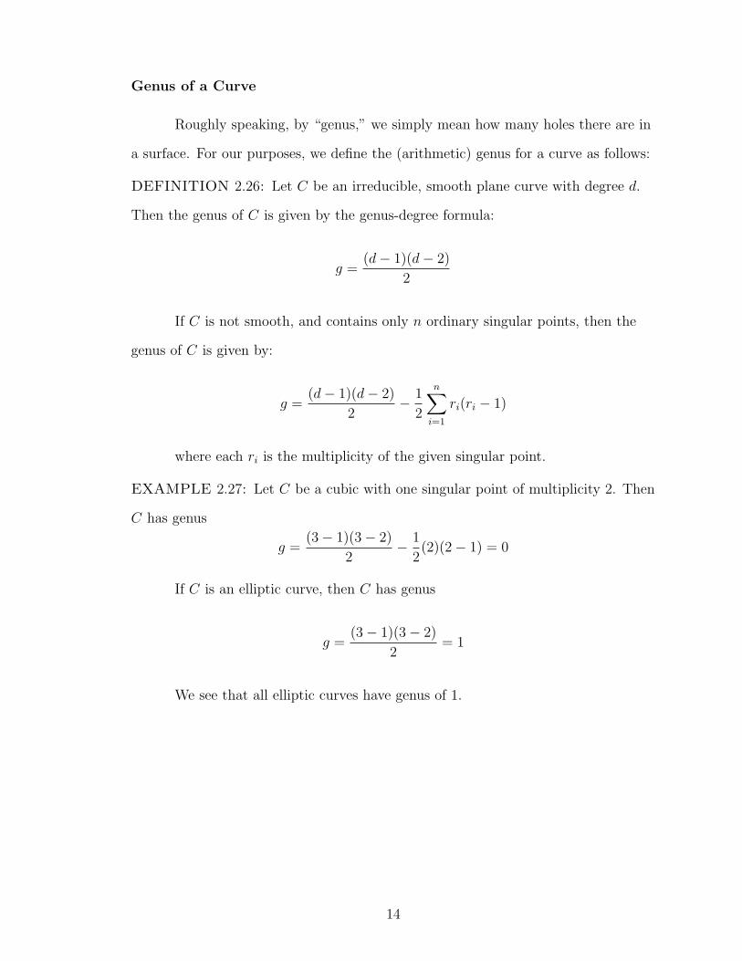
Genus of a Curve

Roughly speaking, by “genus,” we simply mean how many holes there are in

a surface. For our purposes, we define the (arithmetic) genus for a curve as follows:

DEFINITION 2.26: Let C be an irreducible, smooth plane curve with degree d.

Then the genus of C is given by the genus-degree formula:

g =(d− 1)(d− 2)

2

If C is not smooth, and contains only n ordinary singular points, then the

genus of C is given by:

g =(d− 1)(d− 2)

2− 1

2

n∑i=1

ri(ri − 1)

where each ri is the multiplicity of the given singular point.

EXAMPLE 2.27: Let C be a cubic with one singular point of multiplicity 2. Then

C has genus

g =(3− 1)(3− 2)

2− 1

2(2)(2− 1) = 0

If C is an elliptic curve, then C has genus

g =(3− 1)(3− 2)

2= 1

We see that all elliptic curves have genus of 1.

14

3 TAXI CAB PROBLEM AND SUM OF CUBES

The Number 1729

Upon first glance, the number 1729 may appear to be a rather dull number.

As with many other numbers, one may quickly assume that 1729 does not possess

any interesting or awe inspiring properties, outside the well known factoring prop-

erties of number theory. The famous mathematician of the early 20th century, G.

H. Hardy, certainly thought so when he was visiting his friend and colleague, the

equally famous Srinivasa Ramanujan, in the hospital. To Hardy’s surprise, the as-

sumption of the blandness of 1729 was incorrect as is recorded in the following tale,

taken from [6]:

“Once, in the taxi from London, Hardy noticed its number, 1729. He

must have thought about it a little because he entered the room where

Ramanujan lay in bed and, with scarcely a hello, blurted out his disap-

pointment with it. It was, he declared, ‘rather a dull number,’ adding

that he hoped that wasn’t a bad omen. ‘No, Hardy,’ said Ramanujan,

‘it is a very interesting number. It is the smallest number expressible as

the sum of two [positive] cubes in two different ways’”

Ramanujan was famous for his many elegant but highly complex appearing

solutions for mathematical questions; his obscure observation on the above property

of 1729 was not out of place for him. Also not out of place, was the fact that he

was correct. To see how, let’s consider the equation:

x3 + y3 = 1729. (3.1)

Our goal is to show that there exists positive integer solutions (x1, y1) and

15

(x2, y2) such that

x31 + y31 = x32 + y32 = 1729 (3.2)

The process is easier than one might first assume since the expression, x3+y3

is factorable. We have:

x3 + y3 = (x+ y)(x2 − xy + y2). (3.3)

Setting the right hand side of (3.3) equal to 1729 gives:

1729 = (x+ y)(x2 − xy + y2). (3.4)

We now let 1729 = AB for A,B ∈ Z and set

A = x+ y (3.5)

and,

B = x2 − xy + y2. (3.6)

By (3.5), we have y = A− x. Inserting A− x for y in (3.6), we have

B = x2 − x(A− x) + (A− x)2. (3.7)

We know that 1729 = 7 · 13 · 19, and so we can apply this fact to the factor-

ization 1729 = AB, to find positive integer solutions. We do this by taking combi-

nations of the three factors of 1729 and inserting them into (3.6). For example:

16

EXAMPLE 3.1: Take A = 19 and B = 7 · 13 = 91. Then by (3.6), we have

91 = x2 − x(19− x) + (19− x)2

Solving using the quadratic formula, we see that x = 9 and x = 10. Let’s

assume that x = 9. Then y = 10 and so (9, 10) must be a solution to (3.1).

Indeed, 93 + 103 = 1729, and so we have found at least one integer solution

to (3.1).

REMARK 3.2: Example 3.1 really gives us to two solutions to (3.1) since 93 +

103 = 103 + 93 and so both (9, 10) and (10, 9) satisfy (3.1). However, we are inter-

ested in unique solutions to (3.1) and so count (9, 10) and (10, 9) as being the same

solution.

So far, we have only produced one integer solution to x3 + y3 = 1729. Ra-

manujan claimed there was two and no more; we show that he was correct in the

following combinations of A and B values, created using the method above:

A = 91 B = 19

A = 7 B = 247

A = 247 B = 7

A = 13 B = 133

A = 133 B = 13

We see that only A = 13 and B = 133 produce integer solutions when ap-

plied to (3.6). The solution is: (1, 12).

Thus,

93 + 103 = 13 + 123 = 1729.

17

And by the factorization of x3 +y3, we know that the above solutions are the

only possible integer solutions.

REMARK 3.3: The restriction to positive integers is important. If we instead al-

low for the possibility for any integer solution, we would have that the number 91 is

the smallest number expressible as the sum of two cubes since

91 = 63 + (−5)3 = 43 + 33.

As it turns out, while 1729 is the smallest number that can be represented

as the sum of two cubed positive integer, it is not the only number with this prop-

erty. There exists many such numbers, which we represent with the letter r, that

also hold this property. The above discussion is based largely on the arguments

found in [4] and more details on the matter can be found there.

What we have talked about thus far inspires the following definition:

DEFINITION 3.4: The equation α3 + β3 = γ3 + δ3 = r for some integer r is called

a Ramanujan equation if there exists integer pairs (α0, β0) and (γ0, δ0) that satisfy

it. The integer r in this equation is called a Ramanujan number.

The method used earlier to find the solutions to Ramanujan’s problem in-

volved a factorization argument, and was thus purely algebraic. There is almost

always more than one way to solve a mathematical problem, and another way to

solve Ramanujan’s problem is to apply techniques from geometry to it.

The Equation x3 + y3 − z3 − 1 = 0

In this section we assume that we do not know the integer r that satisfies

Definition 3.4. We develop methods to uncover r, even showing another way at

finding the case when r = 1729.

18

To begin, we consider the equation

α3 + β3 = γ3 + δ3 (3.8)

where each of the variables are taken to be positive integers.

From this we have

α3 + β3 − γ3 − δ3 = 0. (3.9)

Equation (3.9) is a homogeneous equation in four variables. We can deho-

mogenize (3.9) by dividing both sides of the equation by δ3, i.e.,

α3

δ3+β3

δ3− γ3

δ3− 1 = 0. (3.10)

Setting x = αδ, y = β

δ, and z = γ

δ, the equation in (3.10) becomes:

x3 + y3 − z3 − 1 = 0. (3.11)

Since α, β, γ, and δ were assumed to be positive integers, it follows that x,

y, and z are positive rational numbers.

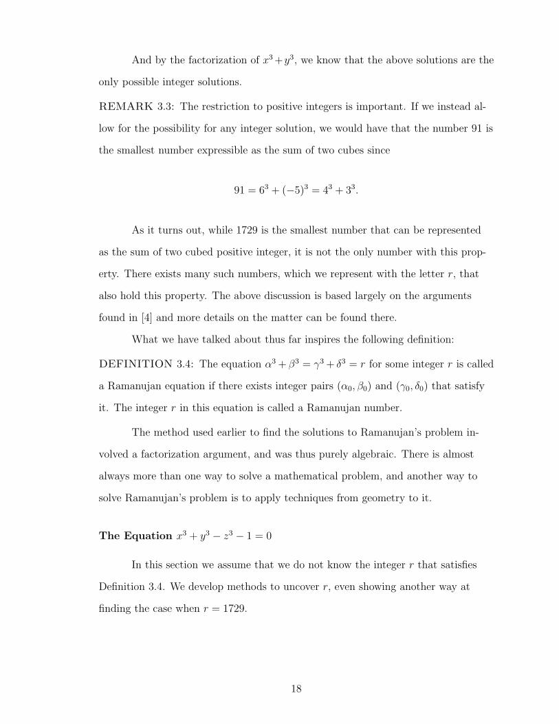
A quick glance at (3.11) shows us that (t, 1, t) is a trivial solution. We know

that on our surface there must be a a line containing these trivial solutions (Fig-

ure 1), and so we take a plane through this line. Slicing our surface in this way will

give us a cubic curve, however, since this line must be a component of the cubic

curve, our end result will be the union of the line and a conic. We can then utilize

this conic to find more solutions to (3.11).

We start by considering a general plane in three-space

px+ qy + rz = s. (3.12)

19

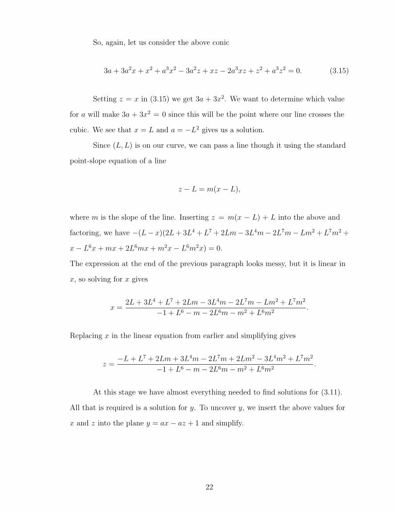
Figure 1: The Surface in (3.11) with Line (t, 1, t)

To determine what the the coefficients are in (3.12), we slice our cubic in

(3.11) with the plane along the line that crosses through a line of trivial solutions

on our cubic. Doing so gives

pt+ q + rt = s. (3.13)

Comparing coefficients across the equation in (3.13) shows

q = s.

Our plane above becomes

px+ qy + rz = q,

20

and dividing both sides of the equation by q gives

p

qx+ y +

r

qz = 1.

We now have our plane written in a form that easily gets us y.

y = −pqx− r

qz + 1.

We also see from equation (3.13) that p = −r. Therefore, letting a = pq

gives

us

y = ax− az + 1. (3.14)

From our work above, we now have a system of equations

x3 + y3 − z3 − 1 = 0,

y = ax− az + 1

Replacing y from the first equation with that found in the second equation

gives

−1 + x3 − z3 + (1 + ax− az)3 = 0.

Factoring the left hand side of the equals sign becomes

(x− z)(3a+ 3a2x+ x2 + a3x2 − 3a2z + xz − 2a3xz + z2 + a3z2) = 0.

As expected with have the line x − z = 0 and a conic. We now consider the

conic in the above equation. From our work earlier in this thesis, we know that we

can create a parameterization for our conic, and thus create as many solutions as

we want for (3.11).

21

So, again, let us consider the above conic

3a+ 3a2x+ x2 + a3x2 − 3a2z + xz − 2a3xz + z2 + a3z2 = 0. (3.15)

Setting z = x in (3.15) we get 3a + 3x2. We want to determine which value

for a will make 3a + 3x2 = 0 since this will be the point where our line crosses the

cubic. We see that x = L and a = −L2 gives us a solution.

Since (L,L) is on our curve, we can pass a line though it using the standard

point-slope equation of a line

z − L = m(x− L),

where m is the slope of the line. Inserting z = m(x − L) + L into the above and

factoring, we have −(L− x)(2L+ 3L4 +L7 + 2Lm− 3L4m− 2L7m−Lm2 +L7m2 +

x− L6x+mx+ 2L6mx+m2x− L6m2x) = 0.

The expression at the end of the previous paragraph looks messy, but it is linear in

x, so solving for x gives

x =2L+ 3L4 + L7 + 2Lm− 3L4m− 2L7m− Lm2 + L7m2

−1 + L6 −m− 2L6m−m2 + L6m2.

Replacing x in the linear equation from earlier and simplifying gives

z =−L+ L7 + 2Lm+ 3L4m− 2L7m+ 2Lm2 − 3L4m2 + L7m2

−1 + L6 −m− 2L6m−m2 + L6m2.

At this stage we have almost everything needed to find solutions for (3.11).

All that is required is a solution for y. To uncover y, we insert the above values for

x and z into the plane y = ax− az + 1 and simplify.

22

We have,

y =−1− 3L3 − 2L2 −m+ 4L6m−m2 + 3L3m2 − 2L2m2

−1 + L6 −m− 2L6m−m2 + L6m2.

If we allow x0, y0, and z0 to represent the solutions for x, y, and z listed

above, we see that

x30 + y30 − z30 − 1 = 0

And thus, the triple (x0, y0, z0) is a solution to x3 + y3 − z3 − 1 = 0.

The fact that (x0, y0, z0) is a solution to our cubic is great news, since we

now have a means to find many numerical solutions to the cubic. Finding these so-

lutions is possible because x0, y0, and z0 are expressed in terms of L and m, which

can be viewed as parameters similar to how t was a parameter in the section on

conics.

We now find some numerical values for x0, y0, and z0. To do this, we first fix

L and allow m to vary. Our L value can be almost anything, but for sake of exam-

ple, we let it equal 2. Then our triple (x0, y0, z0) becomes

(180− 300m+ 126m2

63− 129m+ 63m2,−153 + 255m− 105m2

63− 129m+ 63m2,

126− 204m+ 84m2

63− 129m+ 63m2). (3.16)

With the above solution triple, we are close to having solutions to (3.11).

We recall from earlier that x, y, and z in (3.11) must be positive rational numbers.

To prevent having too many subscripts, let x0, y0, and z0 now take on the respec-

tive coordinates in (3.16). Since (3.11) is cubic, we know that x0, y0, and z0 can all

be positive or z0 can be negative with x0 and y0 having opposite signs. To see this,

consider

(−x0)3 + y30 = (−z0)3 + 1.

23

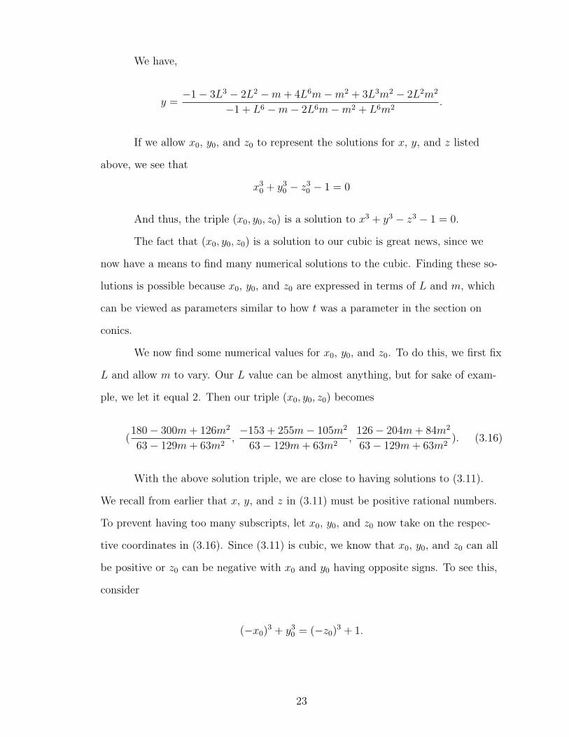
Figure 2: Graphs of x0, y0, and z0

This equation can be re-written as

z30 + y30 = x30 + 1

giving all positive solutions for (3.11).

With this in mind, we plot x0, y0, and z0 as in Figure 2 above to help us see

when the above situations occur. The blue curve in Figure 2 models the x0 coordi-

nate, the yellow curve models y0, and the green curve is the z0 coordinate. We want

to determine values for m that are rational and give us the sign values for x0, y0,

and z0 that we discussed above. From the graph, along with some equation solving,

we see that the interval (.804297, 1.08258) will be the location of m that gives us y0

as positive and the other coordinates as negative. The interval (1.24332, 1.34599)

is where m gives us positive coordinate values. In the second interval above, we

see that an m = 1310

is one rational value for m. This m value gives us the solution

triple (9859, 3559, 9259

). This implies

(98

59

)3

+

(35

59

)3

=

(92

59

)3

+ 1.

24

We find the solutions for the Ramanujan equation by multiplying the above equa-

tion by its least common denominator, that is, 593. Doing so gives us

983 + 353 = 923 + 593. (3.17)

Calculating 983 + 353 gives us 984067. This means that 984067 is a Ramanujan

number, and it can be written as the sum of two positive integer cubes as seen in

(3.17). In a similar way, an m value of 910

gives a solution triple (−13423, 9523,−116

23)

therefore,

1163 + 953 = 1343 + 233 (3.18)

by our discussion on negative numbers and cubes from earlier. We have that 1343 +

233 = 2418271, giving us 2418271 as a Ramanujan number.

As a grand finale, if we let m = 54, we get the solution triple

(10, 9, 12)

Which are the solutions from Ramanujan’s story since, as we know, 103 +

93 = 123 + 13, and of course, these cubes add to 1729.

Thus, we have presented a purely geometric way at finding r values that cor-

respond to those conditions found in Definition 3.4.

25

4 SUMS OF FOURTH POWERS IN TWO DIFFERENT WAYS

The story discussed in the beginning of the previous section is fairly well-

known. However, it is not complete. According to Hardy, after Ramanujan saved

1729 from a mundane life by stating that it had some interesting properties to it,

Hardy asked him if there was any positive integer that could be written as the sum

of two fourth-powers, in two different ways. Sadly for Hardy, Ramanujan did not

know the answer. In this section, we answer Hardy’s question.

We begin in a similar way to the last chapter, but instead of dealing with a

third-degree equation, we have the following fourth-degree equation:

α4 + β4 = γ4 + δ4. (4.1)

As before, we can divide both sides of the equation by δ4 and make appro-

priate substitutions using x, y, and z as new variables to turn (4.1) into

x4 + y4 = z4 + 1.

Which implies

x4 + y4 − z4 − 1 = 0. (4.2)

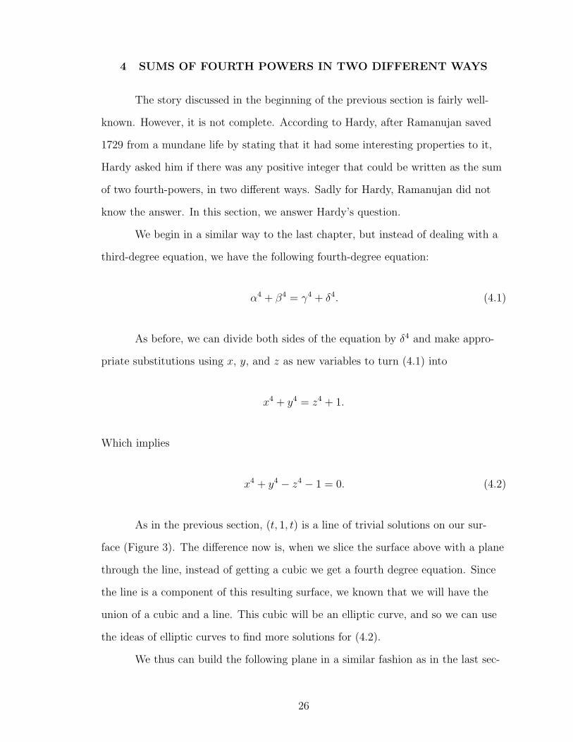
As in the previous section, (t, 1, t) is a line of trivial solutions on our sur-

face (Figure 3). The difference now is, when we slice the surface above with a plane

through the line, instead of getting a cubic we get a fourth degree equation. Since

the line is a component of this resulting surface, we known that we will have the

union of a cubic and a line. This cubic will be an elliptic curve, and so we can use

the ideas of elliptic curves to find more solutions for (4.2).

We thus can build the following plane in a similar fashion as in the last sec-

26

Figure 3: Graph of (4.2) with Line (t, 1, t)

tion:

y = ax− az + 1. (4.3)

Inserting (4.3) into (4.2) and factoring gives (x− z)(4a+ 6a2x+ 4a3x2 + x3 +

a4x3 − 6a2z − 8a3xz + x2z − 3a4x2z + 4a3z2 + xz2 + 3a4xz2 + z3 − a4z3 = 0. We

see that we have recovered our line (x− z) = 0 and the expected cubic. We consider

only the cubic, i.e.,

4a+ 6a2x+ 4a3x2 + x3 + a4x3 − 6a2z − 8a3xz + x2z−

3a4x2z + 4a3z2 + xz2 + 3a4xz2 + z3 − a4z3 = 0.

(4.4)

We have that (4.4) is an elliptic curve. To see this, let F (x, z) be the left

hand side of (4.4). We take partial derivatives on F and arrive at the following set

27

of equations:

∂F

∂x= 6a2 + 8a3x+ 3x2 + 3a4x2 − 8a3z + 2xz − 6a4xz + z2 + 3a4z2 = 0

and,

∂F

∂z= −6a2 − 8a3x+ x2 − 3a4x2 + 8a3z + 2xz + 6a4xz + 3z2 − 3a4z2 = 0.

Attempting to find solutions for x and z that satisfy ∂F∂x

= 0, ∂F∂z

= 0, and

F (x, z) = 0 gives no results, and so F satisfies Definition 2.5.

Finding Solutions

In developing a means of finding solutions to (4.2), we tried two different

approaches. Both approaches are similar in appearance, however, as will be shown

later, only the second approach grants non-trivial solutions.

First Method for Solving (4.2)

The methods used in the previous section for finding solutions to α3 + β3 =

γ3 + δ3 worked very well. Thus, we now attempt to employ similar techniques for

(4.2).

From above, we saw that slicing x4 + y4 − z4 − 1 = 0 with a general plane

through the line (t, 1, t) and constructing the plane y = ax− az + 1, we were able to

produce the elliptic curve (4.4)

We now set P = (t, t) and consider the new point 2P , which we hope will

give us a new, non-trivial point. To find 2P we must first determine the tangent

line that passes through P .

Taking the implicit derivative of (4.4) we have

28

dz

dx=

6a2 + 3x2 + 8a3(x− z) + 3a4(x− z)2 + 2xz + z2

6a2 − x2 + 8a3(x− z) + 3a4(x− z)− 2xz − 3z2. (4.5)

Inserting the point P = (t, t) into (4.5) gives us

a2 + t2

a2 − t2.

Letting m = a2+t2

a2−t2 we form the line

z = m(x− t) + t.

Replacing z in (4.4) with the line above gives us, after factoring and solving,

the following three solutions for x

x = −a13 ,

x = −a13

and,

x = −1

a. (4.6)

The first two solutions above are obvious. The last solution is new and so we

study it more. We see that plugging (4.6) into the line above, we find z = 1a. There-

fore, through similar methods used in the first section, we see that 2P is (− 1a, 1a).

Finally, inserting the x and z values from the respective coordinates of 2P into the

plane y = ax− az + 1 gives y = −1.

While the triple (− 1a,−1, 1

a) is a solution to our equation x4 +y4−z4−1 = 0,

29

multiplying both sides of the equation by a4 gives us

(−1,−a, 1, a)

which is a solution to (4.1), but this a trivial solution.

We have demonstrated that the methods in this section do not grant any

new or interesting points for the equation (4.1), and thus we sought another method

for finding solutions.

The Second Method for Solving (4.2)

Consider, again, the line (t, 1, t). Since our surface is three-dimensional, as

we have already seen, our line must run along our surface. In the previous method,

we could pass infinitely many planes through the line (t, 1, t) which then gave us an

elliptic curve to use. Instead, we now consider a new trivial point for (4.2). There

are many choices for trivial points, but for the sake of example, we use the point

T = (−1, t, t). We then pass a plane through the line (t, 1, t) with the condition

that it also contain T . This reduces the number of planes that we can work with

from infinitely many planes to just one unique plane. By this relation, we see that

our choice for a plane depends on the value for a from the equation y = ax− az+ 1,

or a depends on our value of t.

We consider the case when t depends on a. We set Q = (−1, t) and evaluate

(4.4) at this point. From this, we find that t = 1−a1+a

.

Our unique plane outlined above gives rise to a unique elliptic curve that we

use to calculate what we hope will be a new point. We now find the tangent line

to Q and then consider the third point of intersection of this tangent line on our

elliptic curve. Through similar methods as before, we find the slope of the tangent

line at Q is:

30

1 + 2a+ 6a2 − 2a2 + a4

(−1 + a)2(1 + a)

Letting m = 1+2a+6a2−2a2+a4(−1+a)(1+a) , we can construct the tangent line

z = m(x+ 1) + t

Replacing z in (4.4) with the line above gives us, after factoring and solving,

the following three solutions for x

x = −1

x = −1

and,

x =−1 + 9a+ 8a2 − 6a3 + 23a4 − 3a5 + 2a6

−2 + 3a− 23a2 + 6a3 − 8a4 − 9a5 + a6(4.7)

From Q, we already know x = −1, but the third solution is new. Letting x

be as in (4.7) and inserting this x into the line above shows us that

z =(−1 + a)(−1− 9a+ 8a2 + 6a2 + 23a4 + 3a5 + 2a6

(1 + a)(−2 + 3a− 23a2 + 6a3 − 8a4 − 9a5 + a6

Setting x and z from above into our original plane y = ax − az + 1, we find

that y must be

y =2 + a+ 20a2 − 17a3 + 2a4 − 17a5 + 8a6 + a7

2− a+ 20a2 + 17a3 + 2a4 + 17a5 + 8a6 − a7

Indeed, letting (x0, y0, z0) take on the above values for x, y, and z we see

that that x40 + y40 − z40 − 1 = 0 as desired.

We now have all the information necessary to arrive at various, new solu-

tions to x4 + y4 − z4 − 1 = 0.

31

For example, if we let a = −12, we have the triple ( 76

653), 1203

653, 1176

653) and so

(−67)4 + 1334 = (−59)4 + 1584

REMARK 4.1: We note that, unlike in the case of (3.11), we do not have to con-

cern ourselves with the sign values of our solutions since the degree of each of the

terms in our equation is 4.

Continuing the above process, we see that a value of a = 13

gives (−6779, 133158, −59158

) and

so

764 + 12034 = 11764 + 6534

Finally, a value of a = 2 gives

(−1203)4 + 764 = (−653)4 + 11764

Thus, one can pick various a values and find new solutions for α4 + β4 =

γ4 + δ4 as we have done above.

32

5 THE TETRAHEDRON PROBLEM

There is a classic problem that asks for the side lengths of an equilateral tri-

angle if the distance from the vertices of the triangle are 3, 4, and 5. The answer

turns out to be√

25 + 12√

12. This raises the question: does there exist an equi-

lateral triangle with a side of integer length having a point inside it that is integer

distance from each of the triangles vertices? Christina Bisges, in her master’s thesis

[1], discussed this problem and it’s solution.

We investigate an analogous problem in three dimensions by considering a

tetrahedron. We wish to know if there exists a tetrahedron of integer side length

with a point inside that is integer distance from each of the vertices of the tetrahe-

dron.

By a tetrahedron in the previous paragraph, we mean a solid existing in

three space that is formed by taking four vertices and taking their convex hull. The

type of tetrahedron we will be considering is formulated in the following definition:

DEFINITION 5.1: We say a tetrahedron is regular if its four triangular faces are

composed of congruent triangles. For brevity, we will refer to regular tetrahedrons

as simply tetrahedrons for the remainder of this thesis.

Main Problem

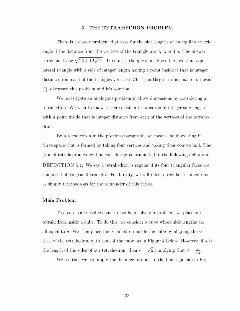
To create some usable structure to help solve our problem, we place our

tetrahedron inside a cube. To do this, we consider a cube whose side lengths are

all equal to u. We then place the tetrahedron inside the cube by aligning the ver-

tices of the tetrahedron with that of the cube, as in Figure 4 below. However, if s is

the length of the sides of our tetrahedron, then s =√

2u implying that u = s√2.

We see that we can apply the distance formula to the line segments in Fig-

33

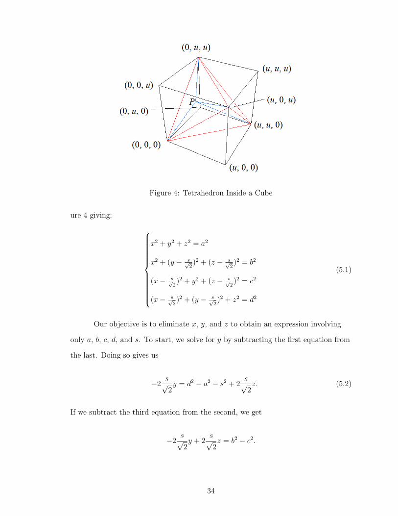
Figure 4: Tetrahedron Inside a Cube

ure 4 giving:

x2 + y2 + z2 = a2

x2 + (y − s√2)2 + (z − s√

2)2 = b2

(x− s√2)2 + y2 + (z − s√

2)2 = c2

(x− s√2)2 + (y − s√

2)2 + z2 = d2

(5.1)

Our objective is to eliminate x, y, and z to obtain an expression involving

only a, b, c, d, and s. To start, we solve for y by subtracting the first equation from

the last. Doing so gives us

−2s√2y = d2 − a2 − s2 + 2

s√2z. (5.2)

If we subtract the third equation from the second, we get

−2s√2y + 2

s√2z = b2 − c2.

34

This shows us that

z =

√2

2s(b2 − c2 + 2

s√2y). (5.3)

If we insert (5.3) into (5.2), we can find a solution for y. We have

−2s√2y = d2 − a2 − s2 + b2 − c2 + 2

s√2y,

which implies,

y =

√2

−4s(−a2 − s2 + b2 − c2 + d2). (5.4)

Inserting the equation for y in (5.4) into (5.2) and solving for z gives us

z =

√2

4s(a2 + b2 − c2 − d2 + s2)

To find x, we consider the equation created by d2 − c2. Taking the equation

found from d2 − c2, inserting the above values for y and z and then solving for x

gives

x =

√2

4s(a2 − b2 − c2 + d2 + s2)

From our work above, we now have x, y, and z expressed in terms of the

side lengths as desired. If we let x0, y0, and z0, we see that the equation x20 + y20 +

z20 − a2 = 0. If we simplify this equation (keeping in mind what x0, y0, and z0 are

equivalent to) gives

3(a4 + b4 + c4 + d4 + s4)

= 2(c2d2 + c2s2 + d2s2 + b2c2 + b2d2 + b2s2 + a2b2 + a2c2 + a2d2 + a2s2)

(5.5)

Much like in the previous section when we dealt with the Taxi Cab problem,

35

our method for finding solutions to the above equation involves de-homegenizng it.

We de-homogenized by dividing the equation by s4. Doing so yields:

3

((a4

s4) + (

b4

s4) + (

c4

s4) + (

d4

s4) + 1

)= 2

(c2d2

s4+c2s2

s4+d2s2

s4+b2c2

s4+b2d2

s4+b2s2

s4+a2b2

s4+a2c2

s4+a2d2

s4+a2s2

s4

) (5.6)

If we set X = as, Y = b

s, Z = c

s, and W = d

s, we see that this change of

variables turns the above equation into

3(X4 + Y 4 + Z4 +W 4 + 1)

= 2(Z2W 2 + Z2 +W 2 + Y 2Z2 + Y 2W 2 + Y 2 +X2Y 2 +X2Z2 +X2W 2 +X2)

(5.7)

We will be making significant use of the above equation, and so for the rest

of this section, instead of using the capital letters found above, we rename our vari-

ables and reuse lower case x, y, z, and w for equation (5.8), i.e.,

3(w4 + x4 + y4 + z4 + 1

)= 2

(w2x2 + w2y2 + w2z2 + w2 + x2y2 + x2z2 + x2 + y2z2 + y2 + z2

) (5.8)

We now discuss three different methods for finding integer solutions for (5.8),

but before we can do so, we must talk about the existence of some singular points.

The Existence of Singular Points

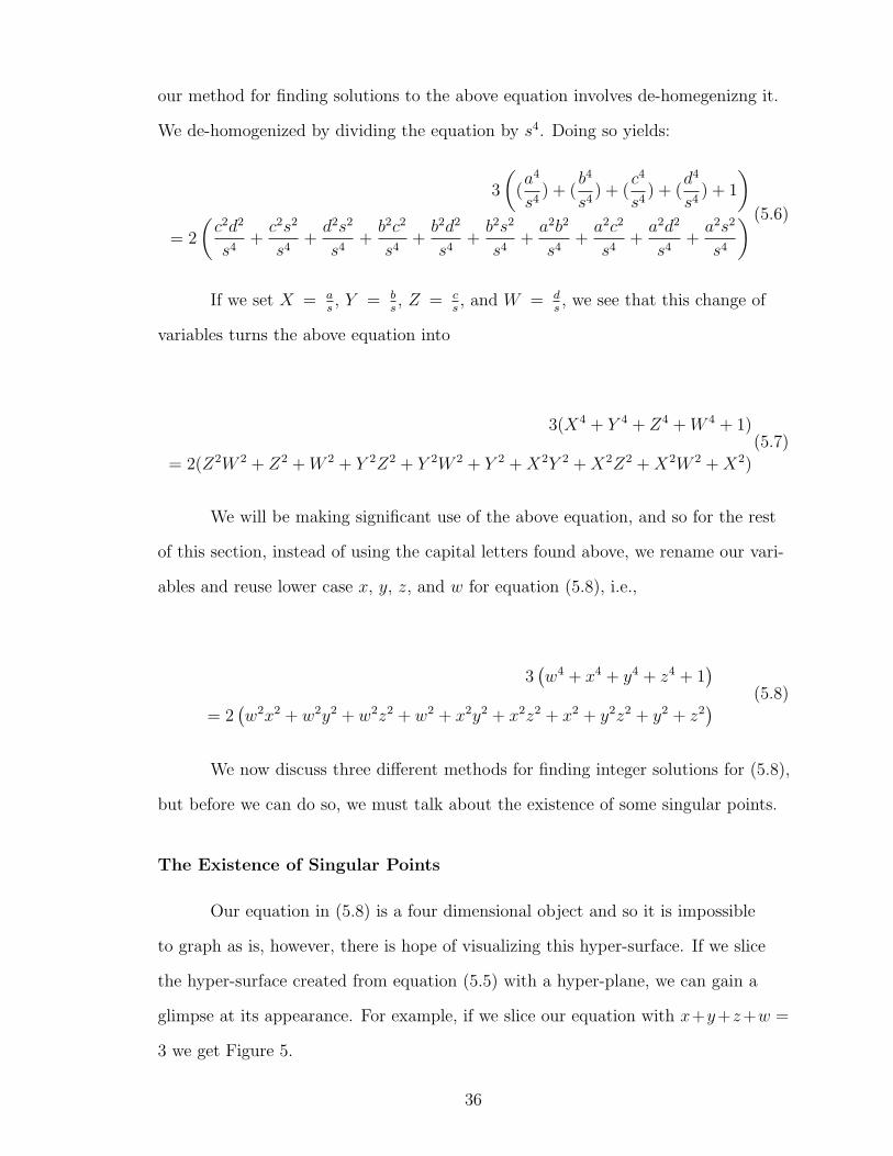
Our equation in (5.8) is a four dimensional object and so it is impossible

to graph as is, however, there is hope of visualizing this hyper-surface. If we slice

the hyper-surface created from equation (5.5) with a hyper-plane, we can gain a

glimpse at its appearance. For example, if we slice our equation with x+y+z+w =

3 we get Figure 5.

36

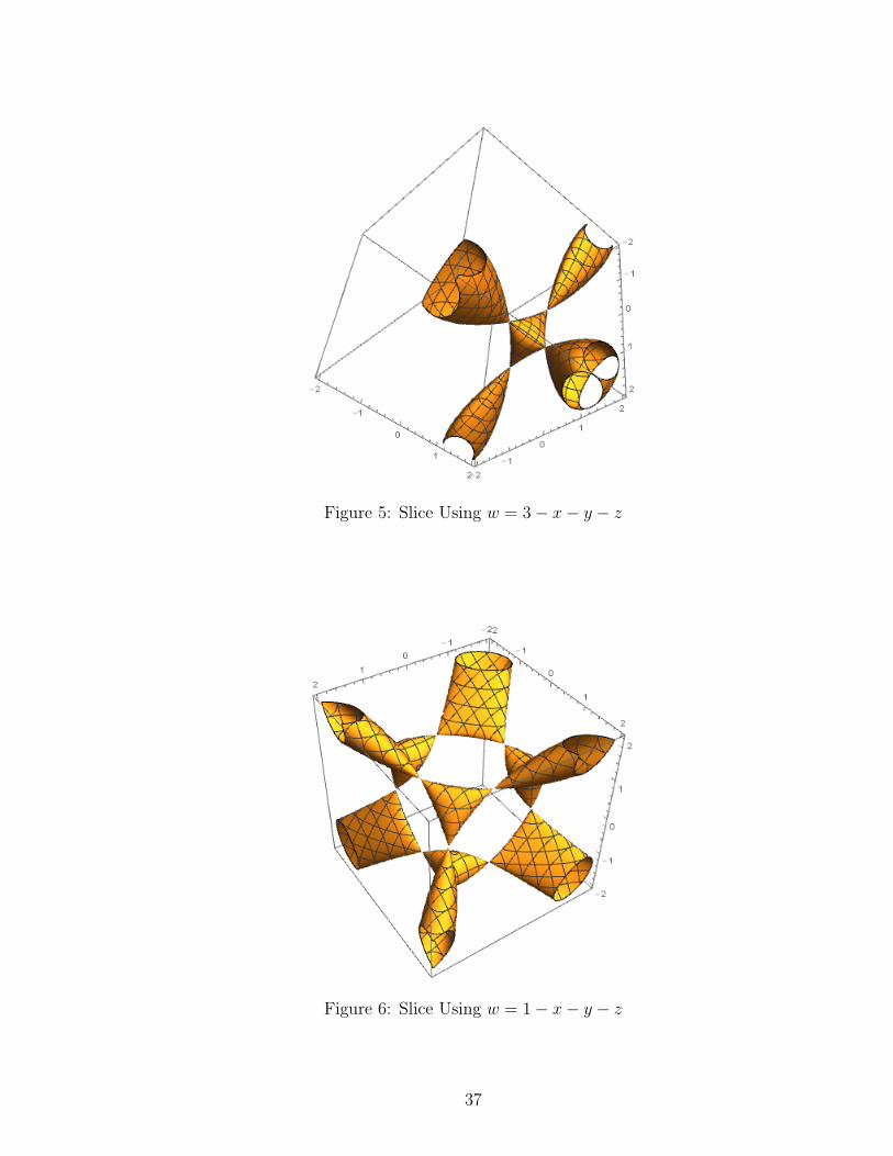
Figure 5: Slice Using w = 3− x− y − z

Figure 6: Slice Using w = 1− x− y − z

37

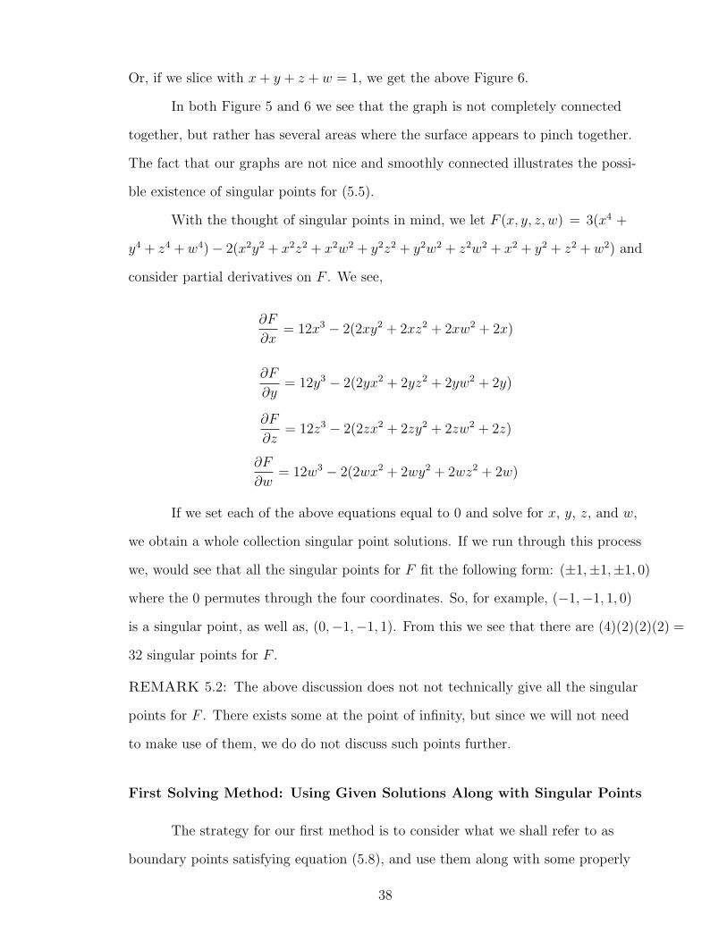
Or, if we slice with x+ y + z + w = 1, we get the above Figure 6.

In both Figure 5 and 6 we see that the graph is not completely connected

together, but rather has several areas where the surface appears to pinch together.

The fact that our graphs are not nice and smoothly connected illustrates the possi-

ble existence of singular points for (5.5).

With the thought of singular points in mind, we let F (x, y, z, w) = 3(x4 +

y4 + z4 +w4)− 2(x2y2 + x2z2 + x2w2 + y2z2 + y2w2 + z2w2 + x2 + y2 + z2 +w2) and

consider partial derivatives on F . We see,

∂F

∂x= 12x3 − 2(2xy2 + 2xz2 + 2xw2 + 2x)

∂F

∂y= 12y3 − 2(2yx2 + 2yz2 + 2yw2 + 2y)

∂F

∂z= 12z3 − 2(2zx2 + 2zy2 + 2zw2 + 2z)

∂F

∂w= 12w3 − 2(2wx2 + 2wy2 + 2wz2 + 2w)

If we set each of the above equations equal to 0 and solve for x, y, z, and w,

we obtain a whole collection singular point solutions. If we run through this process

we, would see that all the singular points for F fit the following form: (±1,±1,±1, 0)

where the 0 permutes through the four coordinates. So, for example, (−1,−1, 1, 0)

is a singular point, as well as, (0,−1,−1, 1). From this we see that there are (4)(2)(2)(2) =

32 singular points for F .

REMARK 5.2: The above discussion does not not technically give all the singular

points for F . There exists some at the point of infinity, but since we will not need

to make use of them, we do do not discuss such points further.

First Solving Method: Using Given Solutions Along with Singular Points

The strategy for our first method is to consider what we shall refer to as

boundary points satisfying equation (5.8), and use them along with some properly

38

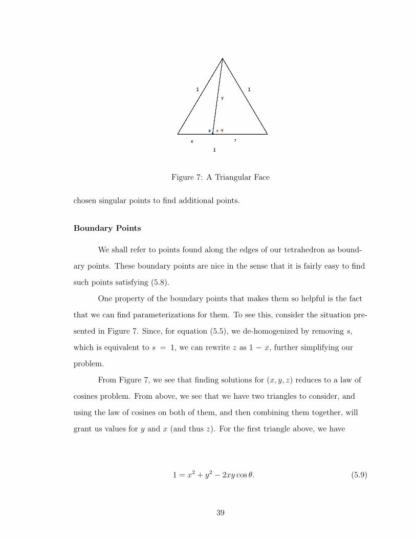
Figure 7: A Triangular Face

chosen singular points to find additional points.

Boundary Points

We shall refer to points found along the edges of our tetrahedron as bound-

ary points. These boundary points are nice in the sense that it is fairly easy to find

such points satisfying (5.8).

One property of the boundary points that makes them so helpful is the fact

that we can find parameterizations for them. To see this, consider the situation pre-

sented in Figure 7. Since, for equation (5.5), we de-homogenized by removing s,

which is equivalent to s = 1, we can rewrite z as 1 − x, further simplifying our

problem.

From Figure 7, we see that finding solutions for (x, y, z) reduces to a law of

cosines problem. From above, we see that we have two triangles to consider, and

using the law of cosines on both of them, and then combining them together, will

grant us values for y and x (and thus z). For the first triangle above, we have

1 = x2 + y2 − 2xy cos θ. (5.9)

39

For the second triangle, the law of cosines gives

1 = (1− x)2 + y2 − 2y(1− x) cos(π − θ). (5.10)

However, since cos(π − θ) = − cos θ, (5.10) becomes

1 = (1− x)2 + y2 + 2y(1− x) cos θ. (5.11)

From (5.9),

cos θ =x2 + y2 − 1

2xy. (5.12)

Inserting (5.12) into (5.11), and simplifying, we get

0 = −2x+ x2 + y2 + 2y(1− x)(x2 + y2 − 1

2xy).

Expanding the above and carrying the x in the denominator of x2+y2−12xy

through-

out, we have

0 = x2 − x− y2 + 1. (5.13)

The equation in (5.13) is a hyperbola, but more importantly, it’s a conic and

so we can create parameterized solutions for it. We mimic the process found in the

section on conics to find the parametrizations we require. Letting x = 0 in (5.13)

gives us a trivial solution of T = (0, 1). We can use T to construct a line that

passes through the hyperbola and thus giving us more solutions. Such a line that

passes through the conic is y = tx + 1, and inserting this line in for y in (5.13) and

40

solving for x gives us

x =2t+ 1

1− t2, t2 6= 1. (5.14)

We can place this above x value into the line y = tx + 1 from earlier to get

us

y =t2 + t+ 1

1− t2, t2 6= 1. (5.15)

Since z = 1− x, we have the triple (2t+11−t2 ,

t2+t+11−t2 ,

−t2−2t1−t2 ) will give us any point

on the boundary of our triangle; we simply need to let t vary to uncover these new

boundary points.

The triple that we just found does more than satisfy points on the bound-

ary, it also gives us a means to find solutions to (5.8). Since each of the triangular

faces on the tetrahedron have the same dimensions, we can determine w in (5.8) by

noting that, in the case of a boundary point, w must equal y.

Therefore, we set w = t2+t+11−t2 , t2 6= 1 and thus, now have a full parameterized

family of degenerate solutions.

Using Degenerate Solutions with Singular Points

We are now prepared to find non-trivial solutions for (5.8). To do so, con-

sider a singular point. Selecting a t value for the parameterizations in the previous

section generates another point, and this point must be rational. We can use these

points to help us find other solutions. One way to determine new points is to con-

struct the line through one of singular points on (5.8) and a boundary point and

then see where else our line intersects the hyper-surface defined by our equation.

Since the degree of a line is 1 and (5.8) has degree of 4, by the Fundamental

Theorem of Algebra, we know that a line should intersect 1× 4 = 4 times.

It can be shown that singular points have a multiplicity of 2, and that any

41

arbitrary non-singular point will have multiplicity 1, therefore a line passing through

a (5.8) must intersect four times, counting multiplicities. Thus far, the line we have

been working with intersects three times (counting multiplicities); our line therefore

must cross (5.8) one more time, and this additional point of intersection must be

rational.

For demonstration purposes, we use for our first singular point, the point

(−1, 1,−1, 0). For our boundary point, we select t = −13

for the parameterizations

in (5.14) and (5.15). This gives the boundary point (38, 58, 78, 78) and the parametric

equation of the line through these points is given by:

x = −1 +5

8p

y = 1− 3

8p

z = −1 +15

8p

w =7

8p

Inserting these values for x, y, z, and w above into (5.8) and factoring gives

1

16(−1 + p)p2(−409 + 469p) = 0

Values of p = 1 and p = 0 are trivial, however, p = 409469

is not trivial and so

we make use of it. If we place p = 409469

into the above equations we have x = −17073752

,

y = 25253752

, z = 23833752

, and w = 409536

. At this point, we have accomplished our goal for

finding solutions to (5.8), since placing our new-found solutions into said equation

grants a value of 0. However, we decided not to stop. There is nothing inherently

special about the boundary points from earlier, save that they are easy to find. We

can use other known points that satisfy (5.8), along with new singular points to

find new solutions.

42

Let us take as our second singular point, the point (1,−1, 1, 0) (we note that

we must use a different singular point each time, otherwise will get back the origi-

nal point we started with). Following the method above, we obtain another set of

parameterized solutions. They are:

x = −1− 5459

3752m

y = −1 +6277

3752m

z = 1− 1369

3752m

w =409

536m

Passing these values above into (5.8) and factoring gives us

57(−1 +m)m2(−791274757 + 549514857m)

1650587344= 0

Again, we don’t really care about m = 1 and m = 0. However, m = 791274757549514857

is non-trivial and so we use it to generate other non-trivial solutions. Placing m =

791274757549514857

into the equations above gives us the solution tuple:

(−4814049371

4396118856,

6194140525

4396118856,

2086406399

4396118856,

4830319039

4396118856) (5.16)

We can repeat the above process multiple times over. However, doing so

quickly generates rather large solutions. For example, using the solution tuple above,

in conjunction with the singular point (0, 1,−1, 1), gives us

x = −51362825753597977184376686449

23499071295923767674102523224

y =42682811754085433189783602535

23499071295923767674102523224

43

z =45665324300355482494525558621

23499071295923767674102523224

and

w =28131709356504504207202399901

23499071295923767674102523224

The numerator and denominators of those fractions contain some huge num-

bers!

We have thus answered our question. We can uncover a, b, c, d, and s from

the fractions above by clearing denominators. For example, for the solution

(−1707

3752,2525

3752,2383

3752,409

536),

found towards the beginning of this current section, we see that upon clearly de-

nominators, a = 1707, b = 2525, c = 2383, d = 2863, and s = 3752. We can preform

a similar process for the other solutions found above.

Second Solving Method: Singular Fourth Degree Curves Intersected with

Conics

In the previous section, we passed a line through one singular point and a

rational point, and then used this line to find more solutions for (5.8). Now, we use

two singular points to find solutions. We slice two hyperplanes through the surface

given by (5.8) in such a way that the hyperplanes pass through both singular points

and a rational point on the surface. This results in a quartic curve with two singu-

lar points and an additional rational point. We wish to intersect this quartic with a

conic in a very special way. This conic must be a member the following set:

Conics = {ax2 + bxy + cy2 + dx+ ey + f = 0, (a, b, c, d, e, f) ∈ Q} (5.17)

Since we are taking our conic to be over Q we can divide by a constant and

44

rewrite the above set as

Conics = {Ax2 +Bxy + Cy2 +Dx+ Ey − 1 = 0, (A,B,C,D,E) ∈ Q} (5.18)

Through dimension counting, any constraint imposed on a conic will lower

its dimension by 1. Thus for the conic that passes through the two singular points

and the rational point, we see that since 3 constraints have been applied, the conic

has dimension 2.

To lower this number even further, we consider both the tangent line and

the second derivative at the rational point, and ask that they agree for the quartic

and the conic, providing two more restrictions to the conic. These additional condi-

tions lowers the dimension to 0 implying a unique conic.

The fact that our conic is unique is powerful since, passing it through two

singular points and a rational point, as well as considering both the tangent line

and second derivative at the rational point means that our conic intersects the sur-

face given by (5.8) 7 times. However, the following theorem tells us more about the

number of times our conic should intersect (5.8).

THEOREM 5.3: (Bezout’s Theorem) [5] Let C1 and C2 be projective curves with

no common components. Then,

∑P∈C1∩C2

I(P, C1 ∩ C2) = (degC1)(degC2)

where I(C1 ∩ C2, P ) is the intersection multiplicity of P defined in the first section.

Thus, we see that the conic must pass through the surface at an additional

point, and as it turns out, this point will be rational.

In order to establish the the two hyperplans necessary for the scheme out-

lined above, we first consider the equation for a general hyperplane in four-space.

We have:

45

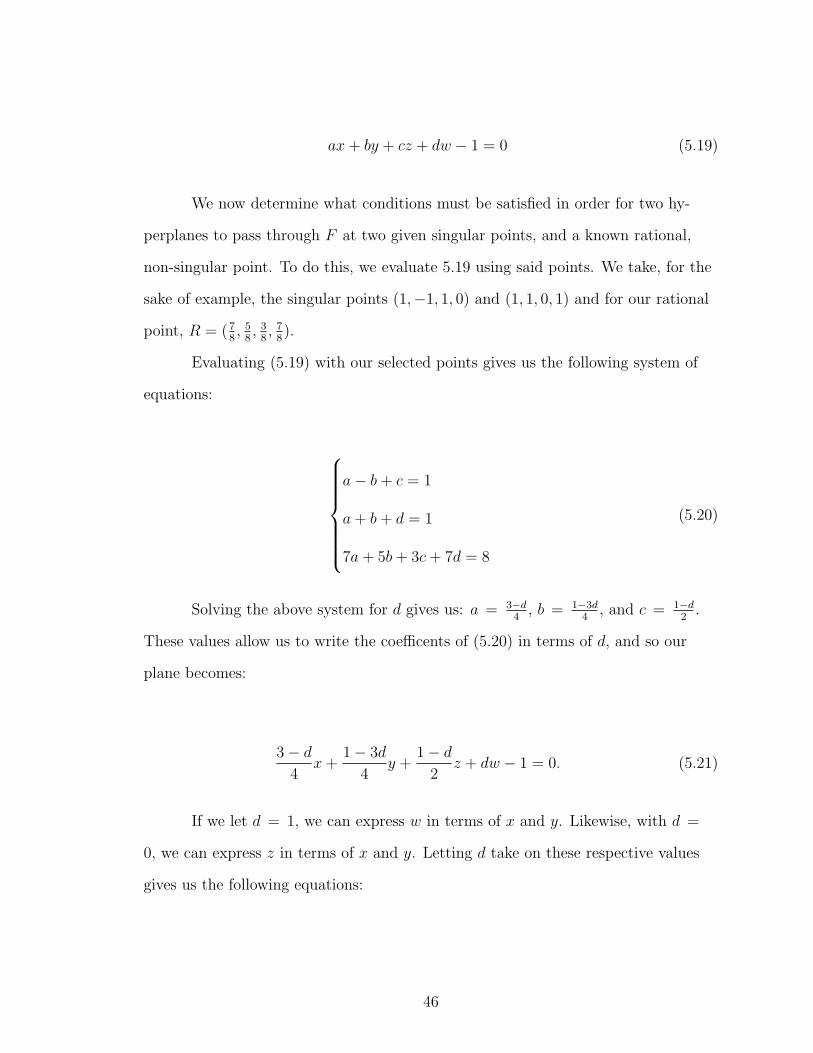
ax+ by + cz + dw − 1 = 0 (5.19)

We now determine what conditions must be satisfied in order for two hy-

perplanes to pass through F at two given singular points, and a known rational,

non-singular point. To do this, we evaluate 5.19 using said points. We take, for the

sake of example, the singular points (1,−1, 1, 0) and (1, 1, 0, 1) and for our rational

point, R = (78, 58, 38, 78).

Evaluating (5.19) with our selected points gives us the following system of

equations:

a− b+ c = 1

a+ b+ d = 1

7a+ 5b+ 3c+ 7d = 8

(5.20)

Solving the above system for d gives us: a = 3−d4

, b = 1−3d4

, and c = 1−d2

.

These values allow us to write the coefficents of (5.20) in terms of d, and so our

plane becomes:

3− d4

x+1− 3d

4y +

1− d2

z + dw − 1 = 0. (5.21)

If we let d = 1, we can express w in terms of x and y. Likewise, with d =

0, we can express z in terms of x and y. Letting d take on these respective values

gives us the following equations:

46

w =2− x+ y

2(5.22)

and,

z =4− 3x− y

2. (5.23)

Placing (5.22) and (5.23) into the equation F (x, y, z, x) = 0, gives us the

curve

3(x4 + (−x2

+y

2+ 1)4 + (−3x

2− y

2+ 2)4 + y4 + 1)−

2((x2((−x2

+y

2+ 1)2 + (−3x

2− y

2+ 2)2 + y2) + x2+

y2((−x2

+y

2+ 1)2 + (−3x

2− y

2+ 2)2) + (−3x

2

− y

2+ 2)2(−x

2+y

2+ 1)2 + (−x

2+y

2+ 1)2 + (−3x

2− y

2+ 2))2 + y2). (5.24)

We now consider the following conic,

px2 + qxy + ry2 + sx+ ty = 1. (5.25)

In order to find when this conic passes through the same points that our

hyperplanes do, we must evaluate it at the same singular points and rational point

from above. The following system of equations result

47

p+ q + r + s+ t = 1

p− q + r + s− t = 1

49p64

+ 35q64

+ 25r64

+ 7s8

+ 5t8

= 1

(5.26)

As mentioned earlier, we want to consider the tangent line at our point R.

However, since R simultaneously exists on both our conic and F , we are forced to

make our tangent line in conjunction with both equations.

For F , using implicit differentiation dydx

and then evaluating the resulting

derivative at the point (78, 58) gives us a value of 3.

Repeating the same process above, only now on the conic grants us,− 7p

4− 5q

8−s

7q8+ 5r

4+t

.

We need this rational expression to equal the slope above, and so we subtract it by

3, giving

−7p4− 5q

8− s

7q8

+ 5r4

+ t− 3. (5.27)

The above becomes:

−2(7p+ 13q + 15r + 4s+ 12t)

7q + 10r + 8t. (5.28)

Subtracting 3 in (5.27) forces (5.28) to be 0. Therefore, the rational expres-

sion in (5.28) equals 0, which implies that it’s numerator is 0. We thus have the

equation

−2(7p+ 13q + 15r + 4s+ 12t) = 0. (5.29)

48

We now find the second derivative at (78, 58), which can be found using the

usual formula.

We have, noting that the value for dydx

must be 3 from our work above, that:

8− 15y′′

8= 0

Therefore, solving for y′′

gives

y′′

=64

15(5.30)

Applying the same process to our conic, we have

2p+ 3q

(7q

8+

5r

4+ t

)y

′′+ 3(q + 6r) = 0

From (5.30), we know the value for y′′. Substituting for y

′′gives

2p+64

15

(7q

8+

5r

4+ t

)+ 3(q + 6r) + 3q = 0 (5.31)

We now have everything needed to find solutions for F .

We arrange all of the above formulas into a system of equations as follows:

p+ q + r + s+ t = 1

p− q + r + s− t = 1

49p64

+ 35q64

+ 25r64

+ 7s8

+ 5t8

= 1

−2(7p+ 13q + 15r + 4s+ 12t) = 0

2p+ 6415

(7q8

+ 5r4

+ t)

+ 3(q + 6r) + 3q = 0

(5.32)

The system of equations in (5.32) contains five equations, and five unknowns.

49

This means that we can solve for the respective unknowns; doing so, and then ap-

plying found values for p, q, r, s, and t, we get the following, unique conic

−13x2

8+

5xy

12+

31x

12+y2

24− 5y

12− 1 = 0 (5.33)

We can now solve for y by eliminating x between the conic in (5.33) and F .

Doing so gives: 356352y8−1024000y7+372096y6+1544000y5−1726373y4−16000y3+

911050y2 − 504000y + 86875 = 0. Factoring gives us

(y − 1)2(y + 1)2(8y − 5)3(696y − 695) = 0

We see that we are successful! We have generated a new, non-trivial point

for F that is rational. Plugging y = 695696

into the conic in (5.33), gives

−13x2

8+

25051x

8352− 15980159

11625984= 0 (5.34)

We find that x = 589696

and x = 20872088

. However, if we plug these x values, along

with our solution for y above, into F , we see that only x = 589696

will work for us.

Placing x = 589696

and y = 695696

into (5.22) and (5.23) from earlier gives us w = 749696

and z = 161696

. Placing these new found values for x, y, z, and w into F gives us 0,

proving that we have found solutions for our equation.

Thus, we have again answered our question posed in the beginning of this

section, this time we will have an tetrahedron of integer side length s = 696 pro-

vided a = 589, b = 695, c = 161, and d = 749.

50

Third Solving Method: Tangent Cone

For each one of the singular points of (5.8), we can form a tangent cone from

that singular point. We can then use tangent lines to the singular point to find

more solutions.

We choose the singular point S = (1, 1, 1, 0), and consider what happens

arbitrarily close to S. In other words, we let x = 1 + r, y = 1 + s, z = 1 + t, and

w = u, where r, s, t, and u are taken to be as close as we like to their respective

coordinates of T (without being equal to them). Doing this gives:

3r4 + 12r3 − 2r2s2 − 4r2s− 2r2t2 − 4r2t− 2r2u2+

12r2 − 4rs2 − 8rs− 4rt2 − 8rt− 4ru2 + 3s4 + 12s3 − 2s2t2 − 4s2t− 2s2u2+

12s2 − 4st2 − 8st− 4su2 + 3t4 + 12t3 − 2t2u2 + 12t2 − 4tu2 + 3u4 − 8u2 = 0. (5.35)

To find the tangent cone, we need only consider the quadratic terms in (5.35).

Collecting the quadratic terms above and simplifying gives

3r2 − 2rs− 2rt+ 3s2 − 2st+ 3t2 − 2u2 = 0. (5.36)

Our singular point exists at the bottom of our cone, and so there exists in-

finitely many tangent lines to that point. In addition, each tangent line intersects

with multiplicity 3, giving us another point of intersection. Since a tangent cone is

a quadratic surface, it behaves in a similar way to a quadratic curve, i.e., a conic.

What this means is that once we have a line lying our the tangent cone, we can

obtain infinitely many other lines through similar techniques as preformed with

conics in earlier sections using paremeterization arguments. With this in mind, we

can form a tangent line to the singular point with the following parameterization:

51

x = 1 + sα, y = 1 + rα, z = 1 + tα, w = uα.

Now, from inspection of (5.36), we see that (1, 1, 2, 2) is a solution. We have

the above parameterization become: x = 1 + α, y = 1 + α, z = 1 + 2α, and w = 2α.

Inserting these parameterizations into (5.5) gives us

3(1296α4 + (2α + 1)4 + 2(5α + 1)4 + 1

)−

2(36α2 + (5α + 1)2(36α2 + 1

)+ (5α + 1)2

(36α2 + (5α + 1)2 + 1

)+ (2α + 1)2

(36α2 + 2(5α + 1)2 + 1

))

Factoring the above gives

36α4 = 0 (5.37)

But, (5.37) implies α = 0, which is trivial. We repeat the same process

above and find (2, 5, 5, 6) is another solution for (5.36). This point gives us x =

1 + 2α, y = 1 + 5α, z = 1 + 5α, and w = 6α. Inserting these values into (5.5) gives,

after factoring,

12α3(179α− 16) = 0. (5.38)

Thus, we see that α = 16179

. Inserting this value of α into our above parame-

terizations gives us the following solution

(211

179,259

179,259

179,

96

179

)(5.39)

52

Indeed, inserting the above values for x, y, z, and w into (5.5) gives us 0 as

desired. We have that a tetrahedron must have side lengths of s = 179 to have a

point inside it of integer distance away from the vertices of the tetrahedron, with

said integer distance being given by a = 211, b = 259, c = 259, and d = 96.

53

6 CONCLUSION

We have developed geometric methods for solving several major Diophan-

tine equations. These include the famous Taxi Cab Problem of the mathematician

Ramanujan and an analogous problem to it involving fourth powers. As we saw,

we could use parameterized solutions to a particular conic to give us solutions to

the Taxi Cab problem, while properties of elliptic curves gave us solutions for the

fourth degree problem. In addition to these, we considered a Diophantine equation

that arose from a problem involving a tetrahedron and gave three solving meth-

ods for finding solutions. Our Diophantine equation turned out to be homogeneous,

but to give us a way at finding solutions for it, we de-homogenized it. We then saw

that the first method for solving relied on lines passing through certain points on

the de-homogenized equation, while the second dealt with a particular conic and

was required to simultaneous meet certain conditions that affected both it, and the

equation. The last method considered a tangent cone that formed from one of the

singular points to the de-homogenized equation, and used tangent lines to the sin-

gular point to find solutions. In essence, we saw that for each of our problems, once

one solution was known, we could then find many more solutions (in fact, for most,

infinitely many more solutions), thus showing how powerful the power of geometry

truly can be.

54

REFERENCES

[1] Christina Bisges, Geometric Techniques for Solving a Certain DiophantineEquation, Missouri State University, Springfield MO, 2012.

[2] Robert Bix, Conics and Cubics: A Concrete Introduction to Algebraic Curves(Undergraduate Texts in Mathematics), Springer-Verlag New York, 1998.

[3] William Fulton, Algebraic Curves: An Introduction to Algebraic Geometry,2008, http://www.math.lsa.umich.edu/ wfulton/CurveBook.pdf

[4] Joseph H. Silverman, Taxicabs and Sums of Two Cubes, MAA, 1993.

[5] Joseph H. Silverman, John Tate, Rational Points on Elliptic Curves, Springer-Verlag New York, 1992.

[6] Eric W. Weisstein, 1729, From MathWorld–A Wolfram Web Resource,http://mathworld.wolfram.com/1729.html.

55