A Detrended Fluctuation Analysis of Monthly Sunspot Number Time Series

Surajit Chattopadhyay1, Goutami Chattopadhyay2

1Pailan College of Management and Technology, Kolkata, 2Institute of Radiophysics and Electronics, University of Calcutta, Kolkata

A brief overview of Sunspot

10/10/2022 2ICFUA 2013

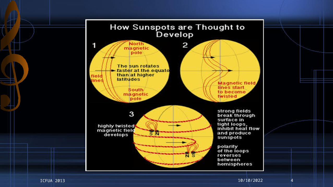
Although the details of sunspot generation are

still a matter of research, it appears that sunspots are the

visible counterparts of magnetic flux tubes in the Sun's convective zone that get "wound up" by differential

rotation.

If the stress on the tubes reaches a certain

limit, they curl up like a rubber band and

puncture the Sun's surface. Convection is

inhibited at the puncture points; the energy flux from the

Sun's interior decreases; and with it surface temperature.

Due to its link to other kinds of solar activity, sunspot occurrence can be used to help predict space weather, the state of the ionosphere, and hence the conditions of short-wave

radio propagation or satellite communications. Solar activity (and the

sunspot cycle) are frequently discussed in the context of global

warming.What is Sunspot?

10/10/2022 3ICFUA 2013

10/10/2022ICFUA 2013 4

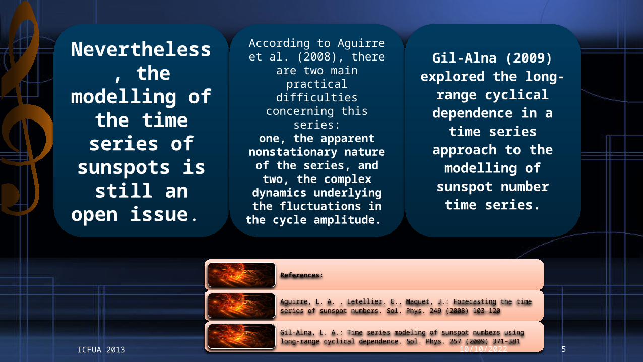
Nevertheless, the

modelling of the time series of sunspots is still an

open issue.

According to Aguirre et al. (2008), there

are two main practical

difficulties concerning this

series:one, the apparent

nonstationary nature of the series, andtwo, the complex

dynamics underlying the fluctuations in

the cycle amplitude.

Gil-Alna (2009) explored the long-range cyclical dependence in a time series

approach to the modelling of sunspot number time series.

References:

Aguirre, L. A. , Letellier, C., Maquet, J.: Forecasting the time series of sunspot numbers. Sol. Phys. 249 (2008) 103–120

Gil-Alna, L. A.: Time series modeling of sunspot numbers using long-range cyclical dependence. Sol. Phys. 257 (2009) 371–381

10/10/2022 5ICFUA 2013

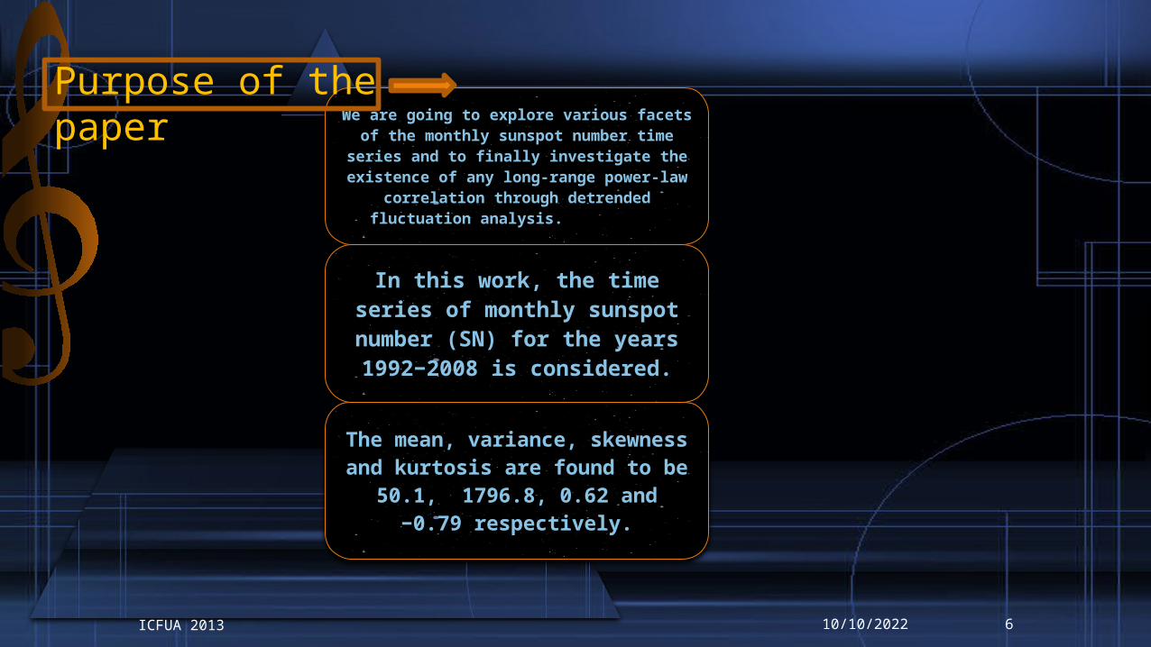
We are going to explore various facets of the monthly sunspot number time

series and to finally investigate the existence of any long-range power-law

correlation through detrended fluctuation analysis. within it.

In this work, the time series of monthly sunspot number (SN) for the years 1992−2008 is considered.

The mean, variance, skewness and kurtosis are found to be

50.1, 1796.8, 0.62 and −0.79 respectively.

Purpose of the paper

10/10/2022 6ICFUA 2013

An overview of Detrended

Fluctuation Analysis (DFA)

10/10/2022 7ICFUA 2013

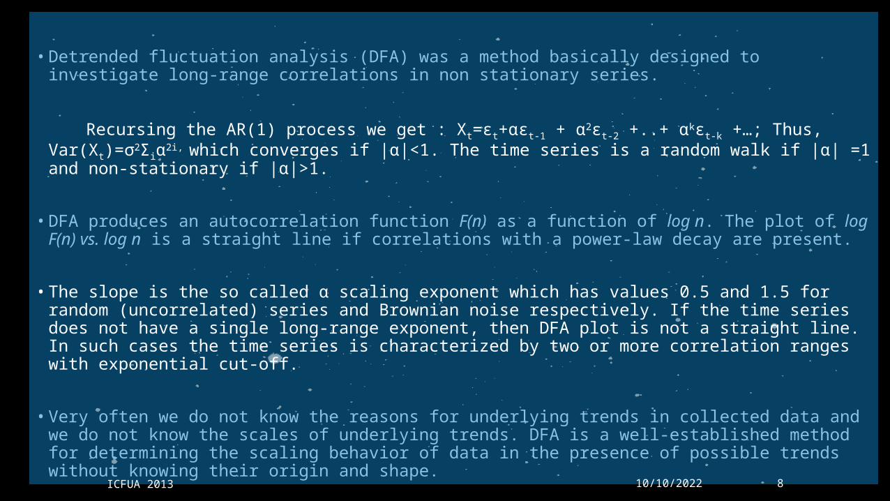
•Detrended fluctuation analysis (DFA) was a method basically designed to investigate long-range correlations in non stationary series.

Recursing the AR(1) process we get : Xt=ϵt+αϵt-1 + α2ϵt-2 +..+ αkϵt-k +…; Thus, Var(Xt)=σ2Σiα2i, which converges if |α|<1. The time series is a random walk if |α| =1 and non-stationary if |α|>1.

•DFA produces an autocorrelation function F(n) as a function of log n. The plot of log F(n) vs. log n is a straight line if correlations with a power-law decay are present.

•The slope is the so called α scaling exponent which has values 0.5 and 1.5 for random (uncorrelated) series and Brownian noise respectively. If the time series does not have a single long-range exponent, then DFA plot is not a straight line. In such cases the time series is characterized by two or more correlation ranges with exponential cut-off.

•Very often we do not know the reasons for underlying trends in collected data and we do not know the scales of underlying trends. DFA is a well-established method for determining the scaling behavior of data in the presence of possible trends without knowing their origin and shape.

10/10/2022 8ICFUA 2013

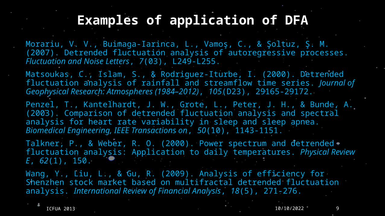
Examples of application of DFAMorariu, V. V., Buimaga-Iarinca, L., Vamoş, C., & Şoltuz, Ş. M. (2007). Detrended fluctuation analysis of autoregressive processes. Fluctuation and Noise Letters, 7(03), L249-L255.Matsoukas, C., Islam, S., & Rodriguez‐Iturbe, I. (2000). Detrended fluctuation analysis of rainfall and streamflow time series. Journal of Geophysical Research: Atmospheres (1984–2012), 105(D23), 29165-29172.Penzel, T., Kantelhardt, J. W., Grote, L., Peter, J. H., & Bunde, A. (2003). Comparison of detrended fluctuation analysis and spectral analysis for heart rate variability in sleep and sleep apnea. Biomedical Engineering, IEEE Transactions on, 50(10), 1143-1151.Talkner, P., & Weber, R. O. (2000). Power spectrum and detrended fluctuation analysis: Application to daily temperatures. Physical Review E, 62(1), 150.Wang, Y., Liu, L., & Gu, R. (2009). Analysis of efficiency for Shenzhen stock market based on multifractal detrended fluctuation analysis. International Review of Financial Analysis, 18(5), 271-276.

10/10/2022 9ICFUA 2013

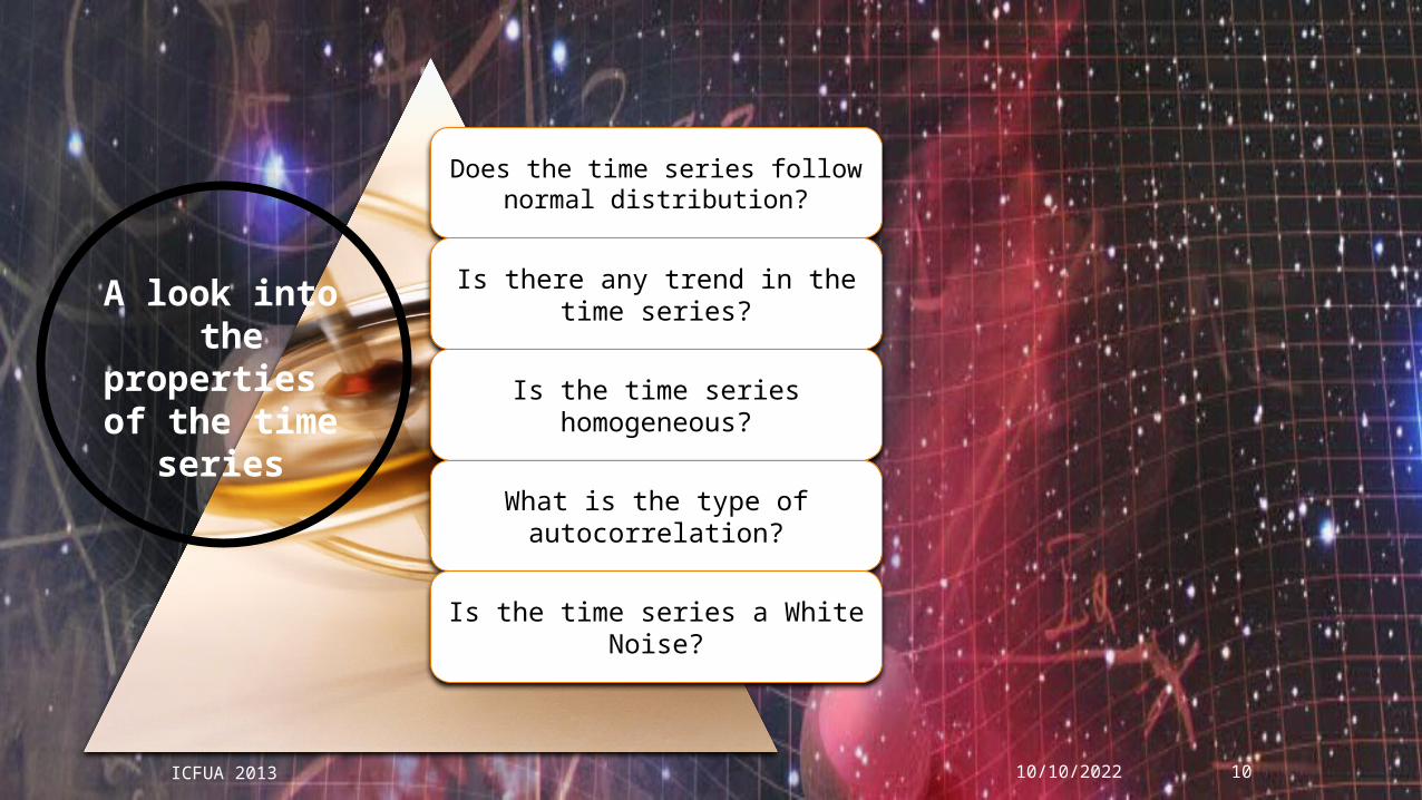
Does the time series follow normal distribution?

Is there any trend in the time series?

Is the time series homogeneous?

What is the type of autocorrelation?

Is the time series a White Noise?

A look into the

properties of the time

series

10/10/2022 10ICFUA 2013

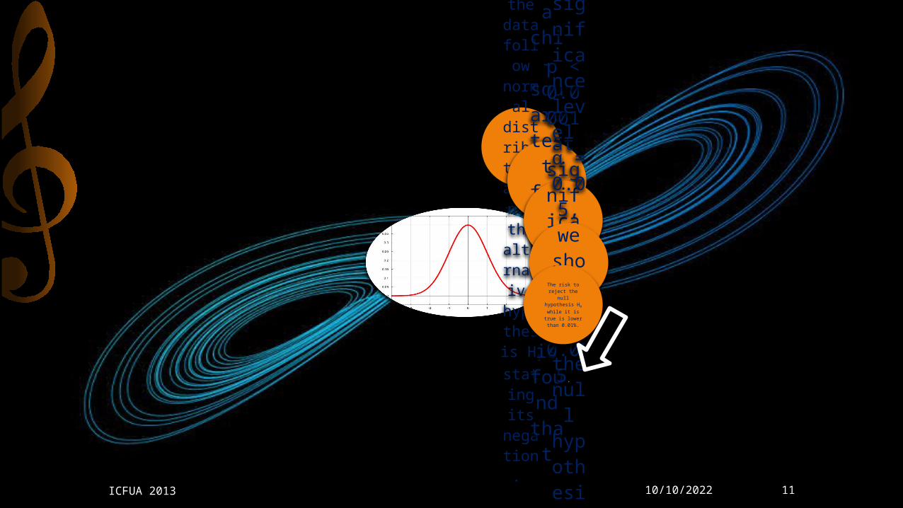
We consider the null hypothesis H0 that the data follow

normal

distribution against the alternative hypothesis H1 stating its negation.

We carry out a

chi-

square test

for H0. Under H0 it is found that

p < 0.0001 at significance level α = 0.05.

As the computed p-value is lower than

the significance level α = 0.05, we should reject the null

hypothesis H0, and accept the alternative hypothesis H1.

The risk to reject the

null hypothesis H0 while it is true is lower than 0.01%.

10/10/2022 11ICFUA 2013

In statistics, homogeneity and its opposite, heterogeneity, arise in describing the properties of a dataset, or several datasets. They relate to the validity of the often convenient assumption that the statistical properties of any one part of an overall dataset are the same as any other part.

In Time series :The initial stages in the analysis of a time series may involve plotting values against time to examine homogeneity of the series in various ways: stability across time as opposed to a trend; stability of local fluctuations over time.

To examine homogeneity of the data

10/10/2022 12ICFUA 2013

A hypothesis test with H0 assuming that the data are homogeneous is tested against alternative hypothesis H1 assuming its negation.

This test is a non-parametric rank test. The ranks r1, ..., rn of the x1, ..., xn are used to calculate the statistic

If a break occurs at time point E, then the statistic is maximal or minimal at E.

In the present case XE = 6798.00 and the two-tailed p-value is < 0.0001. As the computed p-value is lower than the significance level α = 0.05, we should reject the null hypothesis H0, and accept the alternative hypothesis. Thus, we infer that the time series under consideration is not homogeneous.

10/10/2022 13ICFUA 2013

Class centroids in the heterogeneous time series:

Since the entire data-set is not homogeneous, let us try to create clusters within which there are homogeneity. Homogeneity is measured here

using the sum of the within-class

variances.

In this univariate clustering, the

Euclidean distances between

the class centroids of the time series is given by the

matrix

The centroid is the point with the lowest average (squared) distance to all the examples in the cluster. k-means clustering are the most commonly used algorithms for this type of clustering

five class centroids are 10.292, 43.333, 73.904,

103.711 and 133.279 respectively.

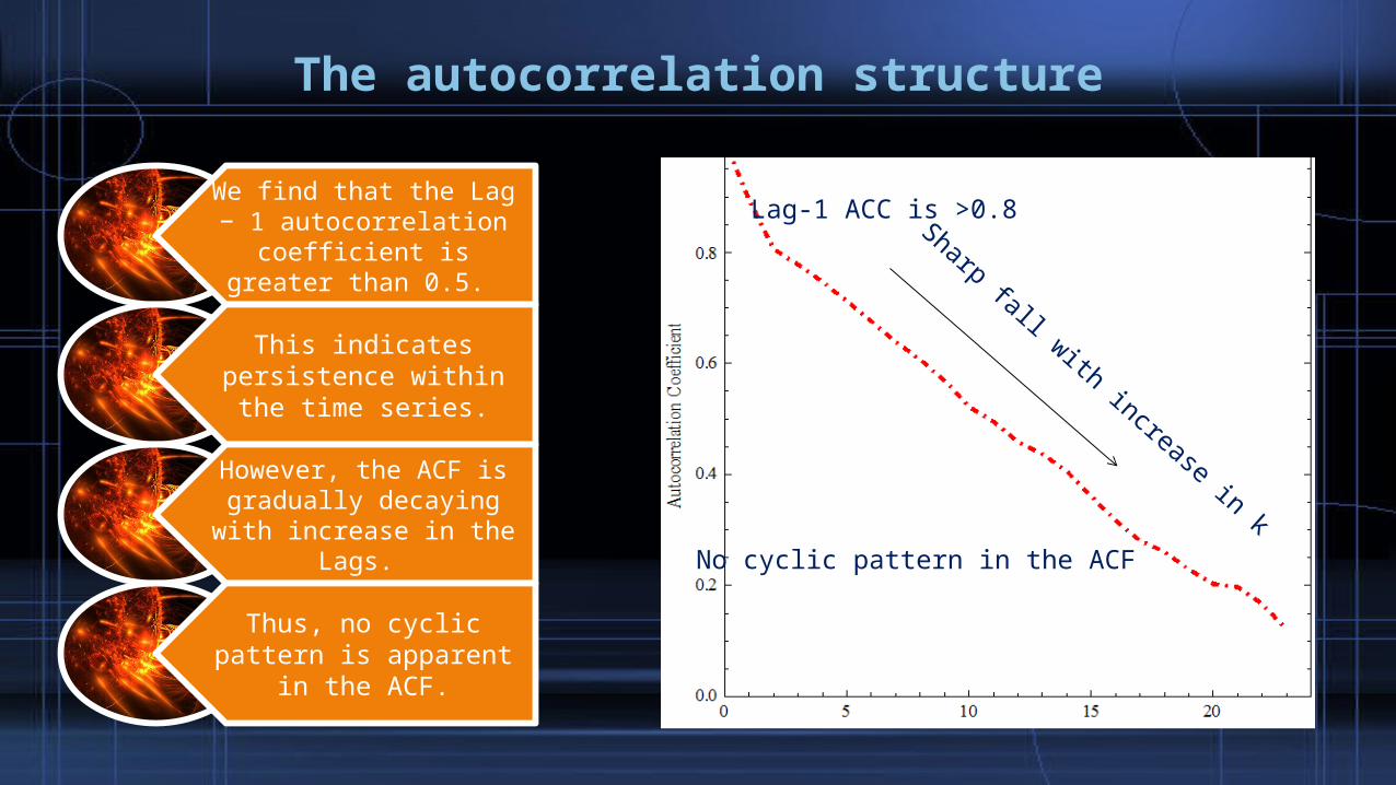
The autocorrelation structure

We find that the Lag − 1 autocorrelation

coefficient is greater than 0.5.

This indicates persistence within the time series.

However, the ACF is gradually decaying with increase in the

Lags.

Thus, no cyclic pattern is apparent

in the ACF.

Lag-1 ACC is >0.8Sharp fall with increase in kNo cyclic pattern in the ACF

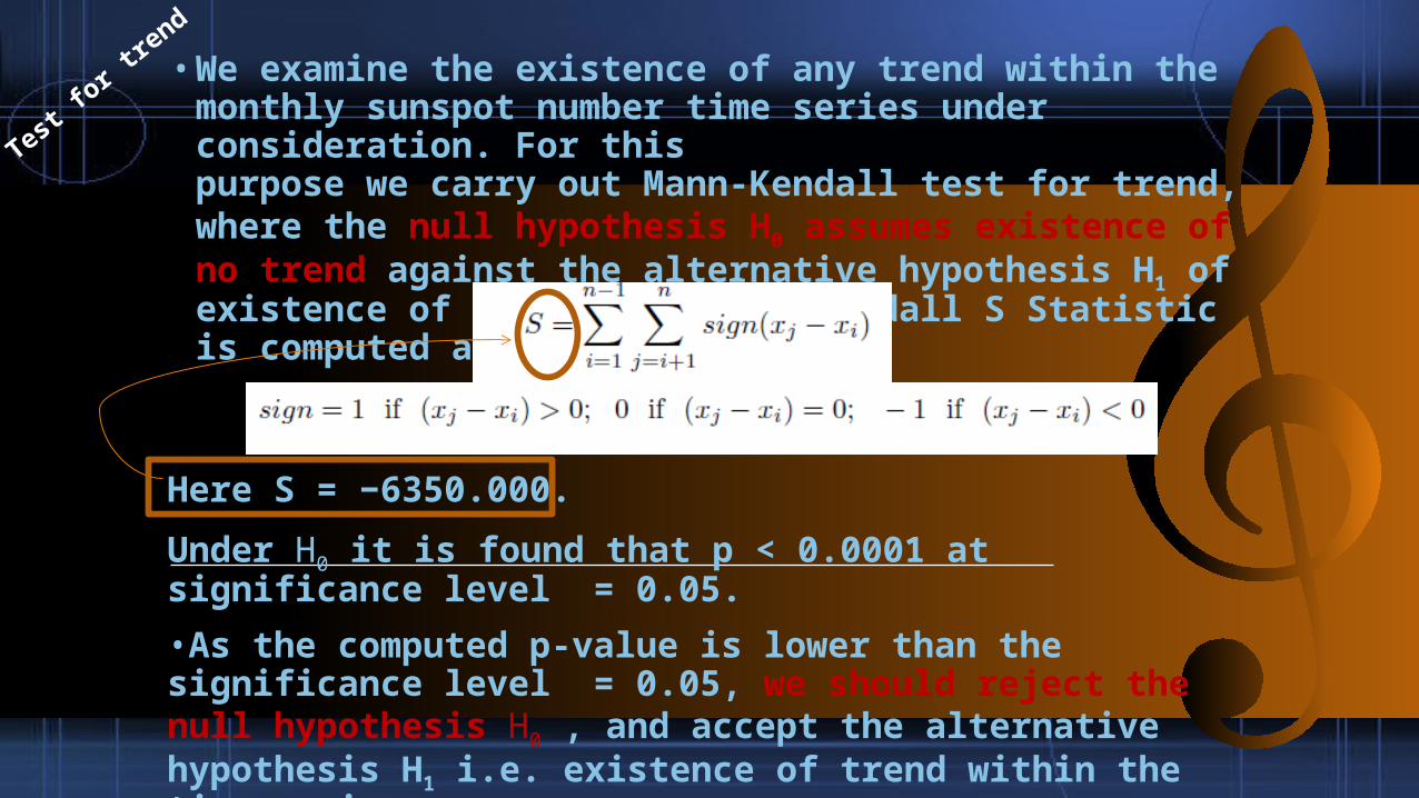
•We examine the existence of any trend within the monthly sunspot number time series under consideration. For thispurpose we carry out Mann-Kendall test for trend, where the null hypothesis H0 assumes existence of no trend against the alternative hypothesis H1 of existence of trend. The Mann-Kendall S Statistic is computed as follows:

Here S = −6350.000. Under H0 it is found that p < 0.0001 at significance level = 0.05. •As the computed p-value is lower than the significance level = 0.05, we should reject the null hypothesis H0 , and accept the alternative hypothesis H1 i.e. existence of trend within the time series.

Test f

or tre

nd

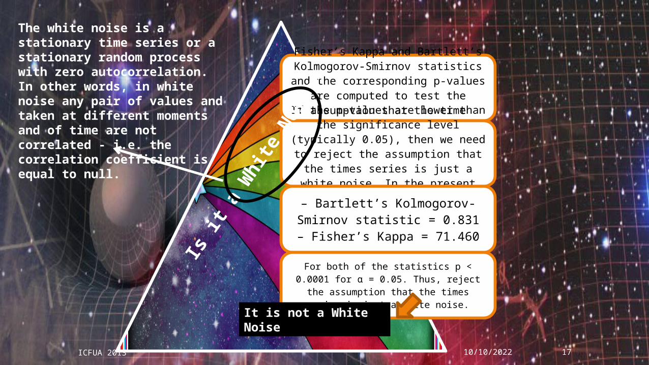
Fisher’s Kappa and Bartlett’s Kolmogorov-Smirnov statistics and the corresponding p-values

are computed to test the assumption that the time

series is just a white noise. If the p-values are lower than

the significance level (typically 0.05), then we need to reject the assumption that the times series is just a white noise. In the present

case,– Bartlett’s Kolmogorov-Smirnov statistic = 0.831– Fisher’s Kappa = 71.460

For both of the statistics p < 0.0001 for α = 0.05. Thus, reject the assumption that the times series is just a white noise.

Is it a White Noise?

The white noise is a stationary time series or a stationary random process with zero autocorrelation. In other words, in white noise any pair of values and taken at different moments and of time are not correlated - i.e. the correlation coefficient is equal to null.

It is not a White Noise

10/10/2022 17ICFUA 2013

The spectral densities are plotted and the plot shows that spikes of different height are occurring at different periods.

Hence, the spectral density is not constant across all frequencies and each frequency in the spectrum does not contributes equally to the variance.

This is consistent with the earlier revealed fact that the time series is not just a white noise.

Spectr

al den

sity i

s sign

ifican

tly va

rying

with p

eriod

10/10/2022 18ICFUA 2013

Thus, the preceeding study shows that– The time series is not Gaussian and positively

skewed;

– The time series is characterized by linear trend through Mann-Kendall’s test;

– The time series is not a white noise process;

– The time series is not homogeneous through Pettitt’s test;

– The time series has five univariate clusters whose centroids are separated by Euclidean

distance ≥ 30;

– The spectral densities have spikes at non-uniform time periods.

10/10/2022 19ICFUA 2013

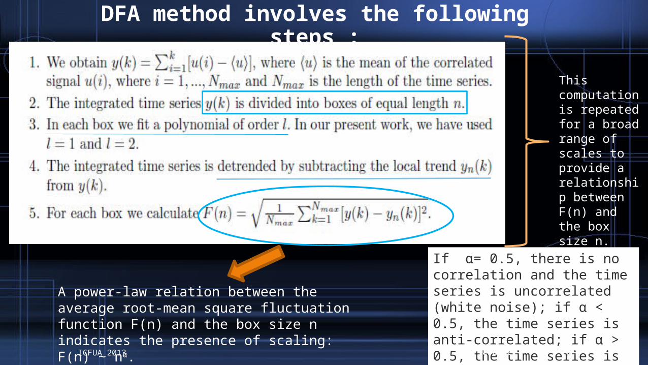
DFA method involves the following steps :

A power-law relation between the average root-mean square fluctuation function F(n) and the box size n indicates the presence of scaling: F(n) ∼ nα.

This computation is repeated for a broad range of scales to provide arelationship between F(n) and the box size n.

If α= 0.5, there is no correlation and the time series is uncorrelated (white noise); if α < 0.5, the time series is anti-correlated; if α > 0.5, the time series is correlated

10/10/2022 20ICFUA 2013

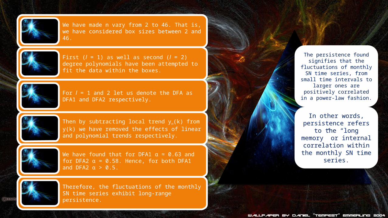
We have made n vary from 2 to 46. That is, we have considered box sizes between 2 and 46.

First (l = 1) as well as second (l = 2) degree polynomials have been attempted to fit the data within the boxes.

For l = 1 and 2 let us denote the DFA as DFA1 and DFA2 respectively.

Then by subtracting local trend yn(k) from y(k) we have removed the effects of linear and polynomial trends respectively.

We have found that for DFA1 α ≈ 0.63 and for DFA2 α ≈ 0.58. Hence, for both DFA1 and DFA2 α > 0.5.

Therefore, the fluctuations of the monthly SN time series exhibit long-range persistence.

The persistence found signifies that the

fluctuations of monthly SN time series, from

small time intervals to larger ones are

positively correlated in a power-law fashion.

In other words, persistence refers

to the “long memory” or internal correlation within the monthly SN time

series.

For a white noise process, α = 0.5. If there are only short-range correlations, the initial slope may be different from 0.5 but will approach 0.5 for large window sizes. Hence the finding is consistent with the earlier finding that the time series is not a white noise process.

DFA1

DFA2

F(n) ∼ n0.63

F(n) ∼ n0.58

0.5 < α < 1.0 indicates the presence of persistent long-range correlations, meaning that a large (compared to the average) value is more likely to be followed by large value and vice versa.

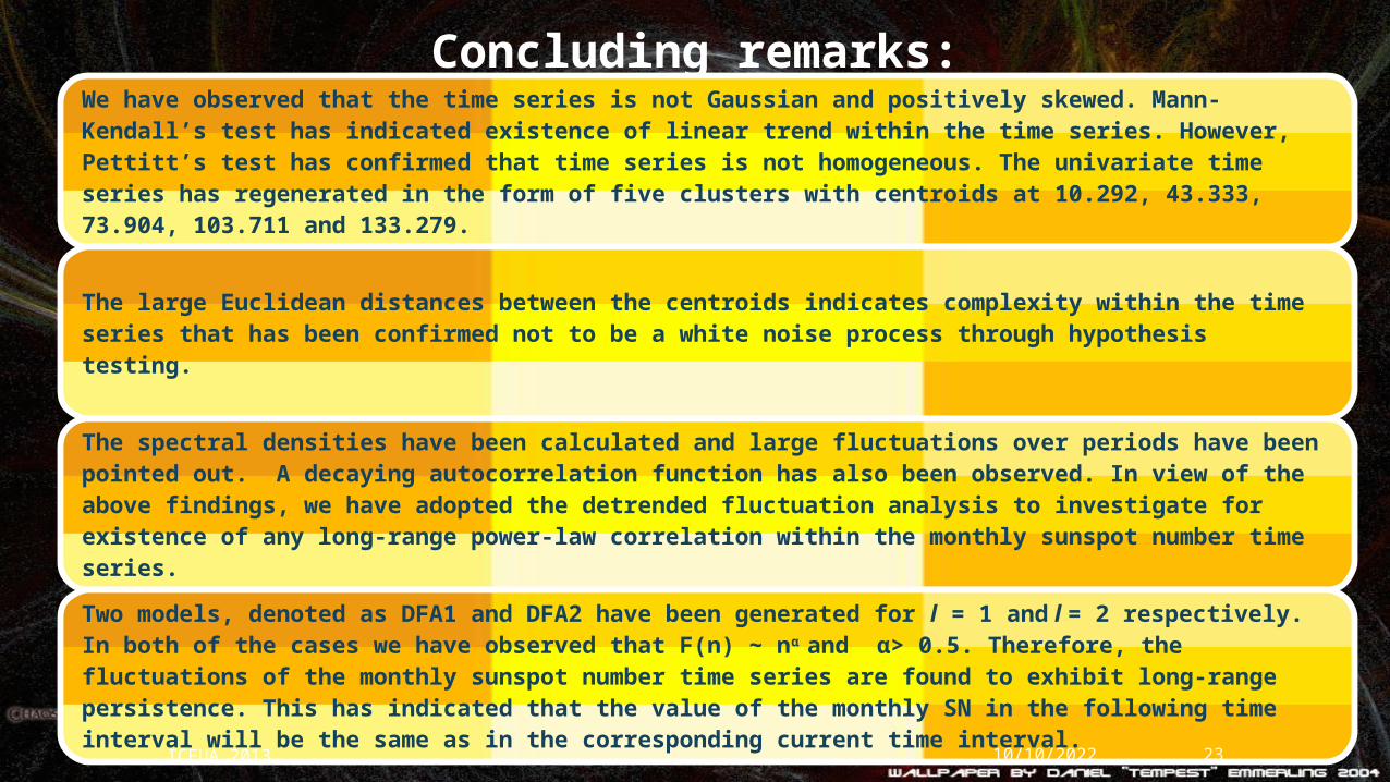
Concluding remarks:We have observed that the time series is not Gaussian and positively skewed. Mann-Kendall’s test has indicated existence of linear trend within the time series. However, Pettitt’s test has confirmed that time series is not homogeneous. The univariate time series has regenerated in the form of five clusters with centroids at 10.292, 43.333, 73.904, 103.711 and 133.279.

The large Euclidean distances between the centroids indicates complexity within the time series that has been confirmed not to be a white noise process through hypothesis testing.

The spectral densities have been calculated and large fluctuations over periods have been pointed out. A decaying autocorrelation function has also been observed. In view of the above findings, we have adopted the detrended fluctuation analysis to investigate for existence of any long-range power-law correlation within the monthly sunspot number time series. Two models, denoted as DFA1 and DFA2 have been generated for l = 1 and l = 2 respectively. In both of the cases we have observed that F(n) ∼ nα and α> 0.5. Therefore, the fluctuations of the monthly sunspot number time series are found to exhibit long-range persistence. This has indicated that the value of the monthly SN in the following time interval will be the same as in the corresponding current time interval.10/10/2022 23ICFUA 2013

References• 1. Noyes, R.W.: The Sun, Our Star (Harvard University Press, Cambridge, 1982).• 2. Chattopadhyay, G., Chattopadhyay, S.: Monthly sunspot number time series analysis and its modeling

through autoregressive artificial neural network. Eur. Phys. J. Plus 127 (2012) Article no. 43• 3. Hu, J., Gao, J., Wang, X.: Multifractal analysis of sunspot time series: the effects of the 11-year

cycle and Fourier truncation. J. Stat. Mech. P02066 (2012) Online at stacks.iop.org/JSTAT/2009/P02066• 4. Aguirre, L. A. , Letellier, C., Maquet, J.: Forecasting the time series of sunspot numbers. Sol.

Phys. 249 (2008) 103–120 • 5. Gil-Alna, L. A.: Time series modeling of sunspot numbers using long-range cyclical dependence. Sol.

Phys. 257 (2009) 371–381• 6. Peng, C. K., Buldyrev, S. V., Havlin, S., Simons, M., Stanley, H. E., Goldberger, A. L.: Mosaic

organization of DNA nucleotides, Phys. Rev. E, 49 (1994) 1685–1689• 7. Varotsos, C.: Power-law correlations in column ozone over Antarctica. Int. J. Remote Sens. 26 (2005)

3333–3342 • 8. Varotsos, C.: The southern hemisphere ozone hole split in 2002. Environ. Sci. Pollut. Res. 9 (2002)

375–376• 9. Varotsos, C., Assimakopoulos, M.-N., Efstathiou, M.: Long-term memory effect in the atmospheric CO2

concentration at Mauna Loa. Atmos. Chem. Phys. 9 (2007) 629–634• 10. Chakraborty, P., Chattopadhyay, G., Chattopadhyay, S.: Investigation of power-law correlations

within daily total ozone time series and search for a stable node through phase portrait. C. R. Geoscience 345 (2013) 55–61

• 11. Kantelhardt, J. W., Zschiegner, S. A., Koscielny-Bunde, E., Havlin, S., Bunde, A., Stanley, H. E.: Multifractal detrended fluctuation analysis of nonstationary time series. Physica A: Statistical Mechanics and its Applications 316 (2002) 87–114

• 12. Zheng, H., Song, W., Wang, J.: Detrended fluctuation analysis of forest fires and related weather parameters. Physica A: Statistical Mechanics and its Applications 387 (2008) 2091–2099

10/10/2022 24ICFUA 2013

Thank

You

10/10/2022 25ICFUA 2013