Embed Size (px)
Citation preview

A
De-anonymizing clustered social networks by percolation graphmatching
CARLA-FABIANA CHIASSERINI, Politecnico di Torino
MICHELE GARETTO, Universita di Torino
EMILIO LEONARDI, Politecnico di Torino
On-line social networks offer the opportunity to collect a huge amount of valuable information about billions of users. The
analysis of this data by service providers and unintended third parties are posing serious treats to user privacy. In particular,
recent work has shown that users participating in more than one on-line social network can be identified based only on
the structure of their links to other users. An effective tool to de-anonymize social network users is represented by graph
matching algorithms. Indeed, by exploiting a sufficiently large set of seed nodes, a percolation process can correctly match
almost all nodes across the different social networks. In this paper, we show the crucial role of clustering, which is a relevant
feature of social network graphs (and many other systems). Clustering has both the effect of making matching algorithms
more prone to errors, and the potential to greatly reduce the number of seeds needed to trigger percolation. We show these
facts by considering a fairly general class of random geometric graphs with variable clustering level. We assume that seeds
can be identified in particular sub-regions of the network graph, while no a-priori knowledge about the location of the other
nodes is required. Under these conditions, we show how clever algorithms can achieve surprisingly good performance while
limiting the number of matching errors.
CCS Concepts: •Mathematics of computing → Random graphs; Probabilistic algorithms; •Networks → Network
privacy and anonymity; On-line social networks;
Additional Key Words and Phrases: Graph matching, bootstrap percolation, de-anonymization
1. INTRODUCTION
On-line social networks have recently emerged as one of the most influential innovations broughtby information and communication technologies, with an enormous impact on social and economicaspects. Due to their popularity, the companies running these on-line services can acquire a hugeamount of valuable information that can be extracted from the traces of activities performed byusers. Such information can be exploited to construct user profiles, which may serve for targetedadvertisements as well as marketing and social surveys. In this scenario, user privacy is clearlyat stake. In particular, accurate user profiles can be obtained when users are members of differentsocial networks and data extracted from different systems are combined together.
This paper is specifically concerned with the case of an ‘attacker’ trying to identify users be-longing to different on-line social networks (without their consent). Recently, security experts havemade the dramatic discovery that user privacy cannot be guaranteed when traces of communicationactivities are made available after applying the simple anonymization procedure which replaces realID’s by random labels [Narayanan and Shmatikov 2009]. Indeed, the traces of user activities over asocial network can be represented by a ‘contact graph’ in which nodes represent anonymized users,and edges denote who has come in contact with whom. Then, an attacker can execute a graph-matching algorithm on the contact graphs generated by different systems, and identify which labelscorrespond to the same user. In the hardest case, this is feasible by using only the topologies ofthe contact graphs [Pedarsani et al. 2013]. The majority of algorithms proposed so far to achievethis goal, however, exploit an initial set of already matched nodes (called seeds) [Narayanan and
Author’s addresses: C.F. Chiasserini and E. Leonardi, Dipartimento di Elettronica e Telecomunicazioni, Politecnico diTorino, Italy; M. Garetto, Dipartimento di Informatica, Universita’ di Torino, Italy.Permission to make digital or hard copies of all or part of this work for personal or classroom use is granted without feeprovided that copies are not made or distributed for profit or commercial advantage and that copies bear this notice andthe full citation on the first page. Copyrights for components of this work owned by others than ACM must be honored.Abstracting with credit is permitted. To copy otherwise, or republish, to post on servers or to redistribute to lists, requiresprior specific permission and/or a fee. Request permissions from [email protected].© YYYY ACM. 1556-4681/YYYY/01-ARTA $15.00DOI: 0000001.0000001
ACM Transactions on Knowledge Discovery from Data, Vol. V, No. N, Article A, Publication date: January YYYY.
CORE Metadata, citation and similar papers at core.ac.uk
Provided by Institutional Research Information System University of Turin

A:2 C.F. Chiasserini et al.
Shmatikov 2009; Peng et al. 2014; Korula and Lattanzi 2014; Kazemi et al. 2015a]. This is actuallya realistic case, since some users explicitly link their accounts in different systems ‘for free’.
Significant progress has also been made towards theoretical understanding of the feasibility ofnetwork de-anonymization (in the first place), and of the asymptotic performance of graph match-ing algorithms applied to large systems. Specifically, when the social network is modeled as anErdos–Renyi random graph, it has been shown in [Pedarsani and Grossglauser 2011] that, undermild conditions, users participating in two different social networks can be successfully matched byan attacker with unlimited computation power, even without seeds. Still in the case of Erdos–Renyicontact graphs, in [Yartseva and Grossglauser 2013] the authors have proposed an identificationalgorithm, named PGM, based on bootstrap percolation [Janson et al. 2012], and they have deter-mined the critical seed set size required to successfully trigger the de-anonymization process. Usinga similar approach, more recently the work in [Chiasserini et al. 2016; Bringmann et al. 2014] hasderived the critical seed set size for network de-anonymization when the contact graph exhibits apower-law degree distribution.
Another essential feature of real social networks, namely, clustering, has not been investigatedso far. Interestingly, in [Yartseva and Grossglauser 2013] authors attempted to apply PGM also tohighly clustered random geometric graphs, observing almost total failure (error rates above 50%).This preliminary finding has been the starting point of our work. In this paper, we consider a fairlygeneral model of random geometric graphs that allows us to incorporate various levels of cluster-ing in the underlying social network, without concurrently generating a scale-free structure. By sodoing, we separate the (unknown) impact of clustering from the (known) impact of power law de-gree, going back to the original case of Erdos–Renyi graphs and moving along a totally different,‘orthogonal’ direction.
The main contributions of this work can be summarized as follows.
— Networks characterized by dense clusters may be largely prone to matching errors when wenaively apply the method proposed in [Yartseva and Grossglauser 2013]. Such errors can be mit-igated and asymptotically eliminated by an improved matching algorithm still based on bootstrappercolation.
— Once errors are removed, clustering turns out to have a surprising beneficial effect on the perfor-mance of graph matching, thanks to a wave-like propagation phenomenon that allows to progres-sively identify all nodes starting from a very small, compact set of seeds.
— In contrast with previous results derived for Erdos–Renyi [Yartseva and Grossglauser 2013] andpower-law graphs [Chiasserini et al. 2016], we show that the number of seeds required for networkde-anonymization can increase with the average node degree of the graph.
Our results are qualitatively validated via experiments with synthetic and real social networkgraphs. We emphasize that, although we focus on network de-anonymization, we do not confineour work exclusively to this problem. Indeed, the results derived here have much broader applica-bility, since graph matching is a general problem arising in many different domains, ranging fromcomputer graphics (e.g., [Egozi et al. 2013]) to bioinformatics (e.g., [Singh et al. 2008]).
2. RELATED WORK
Many proposed matching strategies for network de-anonymization are based on heuristic algorithmsand work by progressively expanding the set of already matched nodes, trying to identify all ofthe other nodes [Narayanan and Shmatikov 2009; Peng et al. 2014; Korula and Lattanzi 2014;Kazemi et al. 2015a]. In particular, in their seminal paper Narayanan and Shmatikov [Narayananand Shmatikov 2009] were able to identify a large fraction of users having account on both Twitterand Flickr (with only 12% error ratio). Algorithms based on supervised learning have been pro-posed to de-anonymize social networks by exploiting semantic information (e.g., name, locationand image of users) [Nunes et al. 2012; Abel et al. 2010]. Structure-based similarity (e.g., neighbor-hood structure) has been recognized to be the most important feature in the graph-matching process[Henderson et al. 2011; Backstrom et al. 2007].
ACM Transactions on Knowledge Discovery from Data, Vol. V, No. N, Article A, Publication date: January YYYY.

De-anonymizing clustered social networks by percolation graph matching A:3
Theoretical studies on the asymptotic performance of graph matching algorithms applied to largesystems have appeared in [Pedarsani and Grossglauser 2011; Yartseva and Grossglauser 2013;Kazemi et al. 2015a; Chiasserini et al. 2016; Bringmann et al. 2014; Onaran et al. 2016]. Specifi-cally, [Yartseva and Grossglauser 2013; Kazemi et al. 2015a] have addressed the case where usersare members of two different social networks and the networks are modeled as Erdos–Renyi ran-dom graphs. In [Yartseva and Grossglauser 2013; Kazemi et al. 2015a] the authors propose practicalidentification algorithms based on bootstrap percolation [Janson et al. 2012], which exploit an initialseed set. It is worth mentioning that [Yartseva and Grossglauser 2013] shows an interesting phasetransition phenomenon in the number of seeds that are required for network de-anonymization. Thealgorithm in [Kazemi et al. 2015a] instead can deal with only partial overlapping between the nodesin the two social network graphs and with moderate errors in the initial seed set.
While the above works all exploit the availability of a seed set, [Pedarsani and Grossglauser 2011;Kazemi et al. 2015b; Onaran et al. 2016] show that an attacker with unlimited computation powercan perform de-anonymization even without seeds. In addition, [Kazemi et al. 2015b] considers thecase where there is only partial overlap between the node sets of the two network graphs while[Onaran et al. 2016] generalizes the case of [Pedarsani and Grossglauser 2011] to graphs withcommunity structure. The approach first proposed in [Pedarsani and Grossglauser 2011], whichrelies on the graphs structural information, has been also exploited [Ji et al. 2016] to quantify thefull or partial de-anonymizability of general and real-world graphs.
The results in [Yartseva and Grossglauser 2013], related to a practical identification algorithmbased on bootstrap percolation, have been recently extended to a more realistic case in which contactgraphs are scale-free (power-law) random graphs. In particular, by modeling them as Chung-Lugraphs, [Chiasserini et al. 2016] and [Bringmann et al. 2014] have independently shown that amuch smaller set of seeds is sufficient to trigger the percolation-based matching process originallystudied in Erdos–Renyi graphs.
Finally, an early version of this work has appeared in the conference paper [Chiasserini et al.2015b]. Also, it is worth mentioning that the identification problem is general and spans over dif-ferent application fields [Leordeanu and Hebert 2005; Melnik et al. 2002; Motahari et al. 2013].
3. NOTATION AND PRELIMINARIES
The network de-anonymization problem under study can be formulated as follows. Consider twosocial networks, represented by the graphs G1(V1, E1) and G2(V2, E2), respectively. Both graphsare considered to be sub-graphs of an inaccessible ground-truth graph, GT(V , E), representing theunderlying true social relationships among people.
Without loss of generality, we assume that GT(V, E), G1(V1, E1) and G2(V2, E2) have the same setof nodes (or vertices) with cardinality n, i.e., V1 = V2 = V . This assumption can be easily releasedby seeking to match only the intersection of vertices belonging to G1 and G2 (see [Kazemi et al.2015a] for an analysis with no-coincident node sets in Erdos–Renyi graphs). Similarly to previousworks [Korula and Lattanzi 2014; Pedarsani and Grossglauser 2011; Yartseva and Grossglauser2013; Chiasserini et al. 2016; Bringmann et al. 2014] we assume that edges in G1 and G2 are obtainedby independently sampling each edge of GT with probability1 s. Specifically, each edge in GT isassumed to be (independently) sampled twice, the first time to determine its presence in E1, thesecond time to determine its presence in E2. This model is a reasonable, first-step approximationof real systems and permits obtaining fundamental analytical insights [Yartseva and Grossglauser2013; Bringmann et al. 2014; Kazemi et al. 2015a; Kazemi et al. 2015b]. Moreover, by lookingat temporal snapshots of an email network, authors in [Pedarsani and Grossglauser 2011; Ji et al.2014] have experimentally found that the above assumption of independent edge sampling is largelyacceptable in their scenario.
1Two different sampling probabilities s1 and s2, respectively for G1 and G2, could be considered as well. In Figure 16, weshow some results for s1 = 0.75 and s2 = 0.5.
ACM Transactions on Knowledge Discovery from Data, Vol. V, No. N, Article A, Publication date: January YYYY.
A:4 C.F. Chiasserini et al.
GT
i
j k
l
G1
i1
j1 k1
l1
G2
i2
j2 k2
l2
P(GT)i1, i2
i1, j2i1, k2
i1, l2j1, i2
j1, j2
j1, k2
j1, l2
k1, i2
k1, j2
k1, k2k1, l2
l1, i2
l1, j2
l1, k2
l1, l2
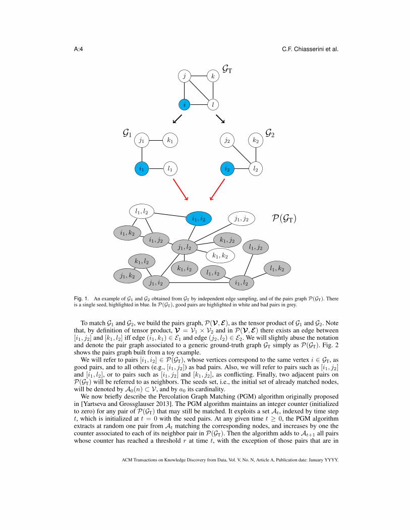
Fig. 1. An example of G1 and G2 obtained from GT by independent edge sampling, and of the pairs graph P(GT). Thereis a single seed, highlighted in blue. In P(GT), good pairs are highlighted in white and bad pairs in grey.
To match G1 and G2, we build the pairs graph, P(V ,E), as the tensor product of G1 and G2. Notethat, by definition of tensor product, V = V1 × V2 and in P(V ,E) there exists an edge between[i1, j2] and [k1, l2] iff edge (i1, k1) ∈ E1 and edge (j2, l2) ∈ E2. We will slightly abuse the notationand denote the pair graph associated to a generic ground-truth graph GT simply as P(GT). Fig. 2shows the pairs graph built from a toy example.
We will refer to pairs [i1, i2] ∈ P(GT), whose vertices correspond to the same vertex i ∈ GT, asgood pairs, and to all others (e.g., [i1, j2]) as bad pairs. Also, we will refer to pairs such as [i1, j2]and [i1, l2], or to pairs such as [i1, j2] and [k1, j2], as conflicting. Finally, two adjacent pairs onP(GT) will be referred to as neighbors. The seeds set, i.e., the initial set of already matched nodes,will be denoted by A0(n) ⊂ V , and by a0 its cardinality.
We now briefly describe the Percolation Graph Matching (PGM) algorithm originally proposedin [Yartseva and Grossglauser 2013]. The PGM algorithm maintains an integer counter (initializedto zero) for any pair of P(GT) that may still be matched. It exploits a set At, indexed by time stept, which is initialized at t = 0 with the seed pairs. At any given time t ≥ 0, the PGM algorithmextracts at random one pair from At matching the corresponding nodes, and increases by one thecounter associated to each of its neighbor pair in P(GT). Then the algorithm adds to At+1 all pairswhose counter has reached a threshold r at time t, with the exception of those pairs that are in
ACM Transactions on Knowledge Discovery from Data, Vol. V, No. N, Article A, Publication date: January YYYY.

De-anonymizing clustered social networks by percolation graph matching A:5
conflict with either any of the already matched pairs or any of the pairs in At. The algorithm stopswhen At = ∅. It is straightforward to see that PGM takes at most n steps to terminate.
Critical seed set size for Erdos-Renyi graphs [Yartseva and Grossglauser 2013].In the case where GT is an Erdos–Renyi random graph2, previous work [Yartseva and Grossglauser2013] has obtained the following result on the critical seed set size ac. We recall that ac is such that:if a0/ac < 1, then only o(n) nodes can be matched, while if a0/ac < 1+ δ, for some δ > 0, almostall nodes can be correctly identified.
LEMMA 3.1. Let GT be an Erdos-Renyi random graph G(n, p). Let r ≥ 4. Denote by ac thecritical seed set size:
ac =
(
1− 1
r
)(
(r − 1)!
n(ps2)r
)1
r−1
. (1)
For n−1 ≪ ps2 ≤ s2n− 3.5r , we have that, if a0/ac < 1 + δ, the PGM algorithm matches w.h.p. a
number of good pairs equal to n − o(n) (i.e., all vertex pairs except for a negligible fraction) withno errors.
In our analysis we assume that s is a positive finite constant (it does not scale with n), thus we omitit whenever we report asymptotic expressions in order sense. Our approach could be extended alsoto the case of vanishing s, but this is out of the scope of this work.Critical seed set size for random graphs bounded by Erdos-Renyi graphs.Let H(V, EH) and K(V, EK) be two random graphs insisting on the same set of vertices V , whereEH ⊆ EK . We define the following partial order relationship:H(V, EH) ≤st K(V, EK).
Then, consider a vertex property R satisfied by a subset of vertices, and denote with R(H) ⊆ Vthe set of vertices of H that satisfy property R. We say that R is monotonically increasing withrespect to the graph ordering relation “≤st” ifR(H) ⊆ R(K) wheneverH ≤st K.
Given that, we present the following results, which complement Theorem 2 and Corollary 3 in[Chiasserini et al. 2016]:
Theorem 1. Consider a subgraph G′T ⊆ GT, which comprises a subset of vertices of GT,whose number is denoted by m, and all the edges between the selected vertices. Assume thatG(m, pmin) ≤st G′T ≤st G(m, pmax) with pmin ≤ pmax. Applying the PGM algorithm to P(G′T)guarantees that m− o(m) good pairs are matched with no errors w.h.p., provided that:
(1) m→∞;(2) pmin = Θ(pmax) and pmin ≫ m−1;
(3) pmax ≤ m− 3.5r , with r ≥ 4;
(4) lim infm→∞ ao/ac > 1, with ac computed from (1) by setting p = pmin.
PROOF. The proof can be found in Appendix C.
Corollary 1. Under the same conditions as in Theorem 1, the PGM algorithm can be success-
fully applied to a pairs graph P ⊂ P(G′T) comprising a finite fraction of the pairs in P(G′T) and
satisfying the following constraint: a bad pair [i1, j2] ∈ P(G′T) is included in P only if either [i1, i2]
or [j1, j2] are also in P .
PROOF. The proof of can be found in [Chiasserini et al. 2016], for completeness a sketch is alsoreported in Appendix D.
2Given a positive integer n and a probability value 0 ≤ p ≤ 1, the Erdos-Renyi graph G(n, p) is defined as the undirectedgraph on n vertices whose edges are chosen as follows. For all pairs of vertices v, w there is an edge (v, w) with probabilityp.
ACM Transactions on Knowledge Discovery from Data, Vol. V, No. N, Article A, Publication date: January YYYY.

A:6 C.F. Chiasserini et al.
The above results provide the basic building blocks to perform the asymptotic analysis of thenumber of seeds that are sufficient to de-anonymize clustered networks described by the modelpresented next.
4. CLUSTERED NETWORK MODEL
To incorporate different degrees of clustering in the ground-truth social network GT, we haveadopted the following geometric random graph model.
We assume that nodes are located in a k-dimensional space corresponding to the hyper-cube3
H = [0, 1]k ⊂ Rk, where the k dimensions could correspond to different attributes of the users. We
consider n nodes independently and uniformly distributed over H. Notice that the node density inthe space is n. Given any two vertices i, j ∈ V , with i 6= j, edge (i, j) exists in GT with probabilitypij that depends only on the Euclidean distance dij between i and j. We consider the followinggeneric law for pij :
pij = K(n)f(dij) . (2)
In (2), f is a non-increasing function of the distance, and K(n) is a normalization constant in-troduced to impose a desired average node degree D(n), which is assumed to be the same for allnodes4. It is customary in random graph models representing realistic systems to assume that theaverage node degree is not constant, but it increases with n due to network densification [Leskovecet al. 2007]. Also, although a common choice is to assume D(n) = Θ(log n), in our model we
consider more general conditions: D(n) = Ω(log n) and D(n) = O(n1/2−δ) with 0 < δ < 1/2.Note that, since D(n)→∞ as n grows large, the graph is connected with high probability.
Since we are interested in the order-sense asymptotic performance of network de-anonymizationas n grows large, we further characterize the shape of function f as follows. Considering that the
average distance between neighboring nodes is equal5 to n−1/k, define C(n) = Ω(
n−1/k)
. We
assume that f(d) equals 1 for all distances 0 < d < C(n), where C(n) is a parameter of the model(possibly scaling with n). Note that this implies that K(n) must be less than or equal to 1, in orderto obtain a proper probability function. For distances larger than C(n), we assume that f decaysaccording to a power-law with exponent β, with β > 0. In summary,
f(dij) = min
1,
(
C(n)
dij
)β
. (3)
thus pij = K(n)min
1, (C(n)/dij)β
. The above characterization of the shape of f(d) is fairlygeneral and allows accounting for different levels of node clustering. In particular, our random-graph model degenerates into a standard Erdos–Renyi graph when either β → 0, with arbitraryC(n), or C(n) approaches 1, with arbitrary β. For β → ∞, instead, edges can be established onlybetween nodes whose distance is smaller than or equal to C(n).
The average node degree is:
D(n) = Θ
(
nK(n)(
Ck(n) + Cβ(n)
∫ 1
C(n)
ρk−1−β dρ)
)
.
From the above equation it follows that for β > k the dominant fraction of the neighbors of a givennode lie at distance Θ(C(n)) from it, while for β < k only a marginal fraction of the neighbors of
3To avoid border effects, we assume wrap-around conditions (i.e., a torus topology).4Note that the node degree distribution is a sum of Bernoulli functions, conditioned on the node position.5We remark that n−1/k is the inverse of the k-th root of the node density in the region H.
ACM Transactions on Knowledge Discovery from Data, Vol. V, No. N, Article A, Publication date: January YYYY.
De-anonymizing clustered social networks by percolation graph matching A:7
a node lie at distance o(1) from it. Thus, we can write:
D(n) =
Θ(
nK(n)Ck(n))
β > k
Θ(
nK(n)Ck(n) log 1C(n)
)
β = k
Θ(
nK(n)Cβ(n))
β < k
(4)
Next, we compute the scaling order of the clustering coefficient6 χ. As shown in Appendix B, wehave:
χ =
Θ(K(n)) β > k
Θ(
K(n)log2[1/C(n)]
)
β = k
Θ(
K(n)C(n)2(k−β))
2k3 < β < k
Θ(
K(n)C(n)β log[1/C(n)])
β = 2k3
Θ(
K(n)C(n)β)
β < 2k3 .
(5)
Looking at χ, we note that in all cases the clustering coefficient of the graph is upper-bounded byK(n) (actually it equals K(n) for β > k). In essence, in our model K(n), C(n) and β providethe three knobs that allow us to directly control the both the average node degree and clusteringcoefficient of the graph. We underline that many real-world networks exhibit a fairly large clusteringcoefficient, as it occurs in our model when β > k.
We remark that, unlike specifically tailored graph models such as stochastic block-models, ourgeometric random graphs do not directly capture the community-based structure exhibited by so-cial networks. However, they successfully represent the clustering effect, which is the main featureinvestigated in this paper.
Note: In the following, we will slightly abuse the language and define as clusters (not to be con-fused with the clustering coefficient) sub-regions including nodes whose maximum mutual distanceis Θ(C(n)).
5. OVERVIEW AND MAIN RESULTS
Our goal is to characterize the seed set necessary for de-anonymization. To this end, we identify twodifferent regimes depending on K(n), which provides the graph density of clusters 7:
1) K(n) = o([nCk(n)]−γ), for some 0 < γ < 1, which will be referred to as low-density clustercase;2) K(n) = ω([nCk(n)]−γ) for any γ > 0, which will be referred to as high-density cluster case.
In the first case, the graph density within a cluster goes to zero “relatively” fast as the number ofnodes within a cluster, nCk(n), goes to infinity. In the second case, the graph density within acluster either is bounded away from zero or asymptotically decreases very slowly. It comprises theparticularly relevant sub-case in which K(n) = Θ(1). Within each of the above cases, differentoperational sub-regimes can be identified based on the value of β/k and B(n) = nK(n)Ck(n).Note that B(n) can be interpreted as the average number of neighbors of a given node within acluster centred at the considered node.
In order to analyze the performance achievable in different cases, we will consider three differentmatching strategies. Note that for all strategies we will assume that seeds can be identified in par-ticular sub-regions ofH, while no knowledge on the location of the other nodes is required to carryon the node identification process.
(i) The simplest approach consists in applying PGM directly to the original pairs graph by usingseeds in an opportunely defined sub-region ofH, and by selecting a proper threshold r. We point out
6Roughly speaking, the clustering coefficient is the probability that two neighbors of a node are neighbors of each other.7Given a generic graph G(V, E), the graph density is defined as
2|E||V|(|V|−1)
. It can be interpreted as the probability that an
edge exists between two randomly selected nodes of the graph.
ACM Transactions on Knowledge Discovery from Data, Vol. V, No. N, Article A, Publication date: January YYYY.
A:8 C.F. Chiasserini et al.
that, in this case, r may scale to infinity as n grows large, as shown in Section 6. Such an approachwill be used when the product B(n) · K(n) is small, for either low or high-density clusters (seeSections 7.2, 7.3, 7.4 and 8.2). Indeed, in these cases, the edge density within a cluster is smallenough to safely apply the PGM algorithm without incurring matching errors.
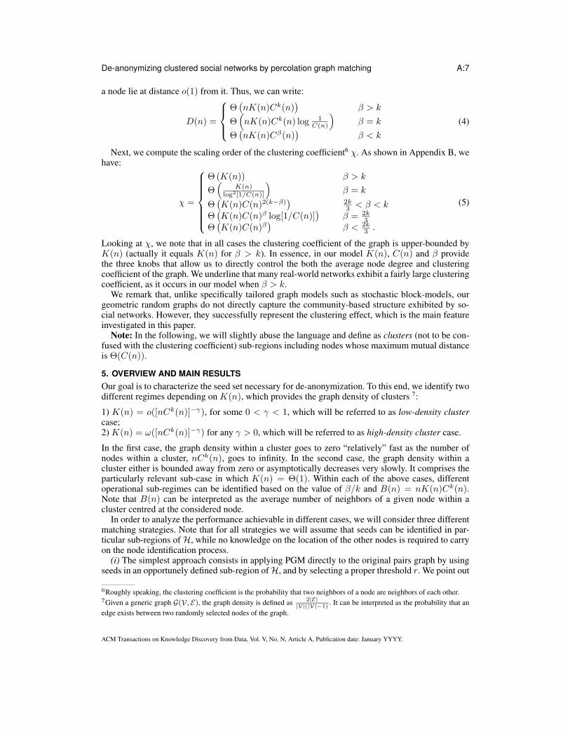
(ii) The second approach implies that initially only a small sub-region of H of size Θ(C(n)) isconsidered. Then the PGM algorithm can be applied to this sub-region8, provided that a sufficientlylarge seed set is available therein and an opportune threshold r is selected. At the end of this first‘trigger phase’ almost all nodes located in the considered region are correctly identified. The set ofmatched pairs is then iteratively expanded, using as seed set the good pairs identified at the previousstage (representing a discretized version of a wave-like expansion). Note that, in this second phase,we do not apply PGM any more, but a simpler direct strategy, matching at each step those pairshaving a sufficiently large number of neighboring pairs matched at the previous steps. Fig. 2 depictsthis approach. This matching procedure will be used to de-anonymize nodes pairs in the case of low-density clusters when B(n) ·K(n) is sufficiently large (Sec. 7.1).
already de-anonimized
to be de-anonymized
next to be de-anonymized
Fig. 2. Graphical representation of matching strategy based on wave-like expansion.
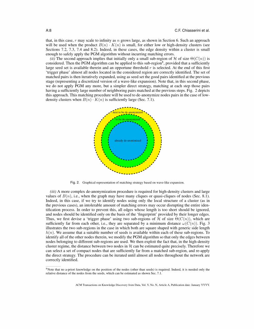
(iii) A more complex de-anonymization procedure is required for high-density clusters and largevalues of B(n), i.e., when the graph may have many cliques or quasi-cliques of nodes (Sec. 8.1).Indeed, in this case, if we try to identify nodes using only the local structure of a cluster (as inthe previous cases), an intolerable amount of matching errors may occur disrupting the entire iden-tification process. In order to prevent this, all edges whose length is too short should be ignored,and nodes should be identified only on the basis of the ‘fingerprint’ provided by their longer edges.Thus, we first devise a ‘trigger phase’ using two sub-regions of H of size Θ(C(n)), which aresufficiently far from each other, i.e., they are separated by a minimum distance ω(C(n)). Fig. 3illustrates the two sub-regions in the case in which both are square shaped with generic side lengthh(n). We assume that a suitable number of seeds is available within each of these sub-regions. Toidentify all of the other nodes therein, we modify the PGM algorithm so that only the edges betweennodes belonging to different sub-regions are used. We then exploit the fact that, in the high-densitycluster regime, the distance between two nodes inH can be estimated quite precisely. Therefore wecan select a set of compact nodes that are sufficiently far from a matched sub-region, and re-applythe direct strategy. The procedure can be iterated until almost all nodes throughout the network arecorrectly identified.
8Note that no a-priori knowledge on the position of the nodes (other than seeds) is required. Indeed, it is needed only therelative distance of the nodes from the seeds, which can be estimated as shown Sec. 7.1.
ACM Transactions on Knowledge Discovery from Data, Vol. V, No. N, Article A, Publication date: January YYYY.
De-anonymizing clustered social networks by percolation graph matching A:9
H1 H2
ω(h(n))
h(n) h(n)
Fig. 3. Graphical representation of trigger phase based on two separated sub-regions of side h(n).
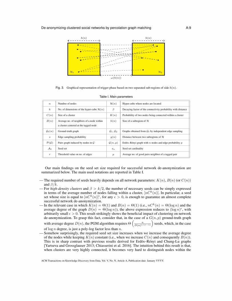
Table I. Main parameters
n Number of nodes H(n) Hyper-cube where nodes are located
k No. of dimensions of the hyper-cube H(n) β Decaying factor of the connectivity probability with distance
C(n) Size of a cluster K(n) Probability of two nodes being connected within a cluster
B(n) Average no. of neighbors of a node within h(n) Size of a subregion of Ha cluster centered at the tagged node
GT(n) Ground-truth graph G1,G2 Graphs obtained from GT by independent edge sampling
s Edge sampling probability g(n) Distance between two subregions of H
P(G) Pairs graph induced by nodes in G G(n, p) Erdos–Renyi graph with n nodes and edge probability p
A0 Seed set ao Seed set cardinality
r Threshold value on no. of edges µ Average no. of good pairs neighbor of a tagged pair
Our main findings on the seed set size required for successful network de-anonymization aresummarized below. The main used notations are reported in Table I.
— The required number of seeds heavily depends on all network parameters: K(n), B(n) (or C(n))and β/k.
— For high-density clusters and β > k/2, the number of necessary seeds can be simply expressedin terms of the average number of nodes falling within a cluster, [nCk(n)]. In particular, a seedset whose size is equal to [nCk(n)]ǫ, for any ǫ > 0, is enough to guarantee an almost completesuccessful network de-anonymization.
— In the relevant case in which K(n) = Θ(1) and B(n) = Θ(1) (i.e., nCk(n) = Θ(log n) and theaverage degree of the graph D(n) = Θ(log n)), the above expression reduces to (log n)ǫ, witharbitrarily small ǫ > 0. This result strikingly shows the beneficial impact of clustering on networkde-anonymization. To grasp this fact, consider that, in the case of a G(n, p) ground-truth graph
with average degree D(n), the PGM algorithm requires Θ(
nD(n)r/(r−1)
)
seeds, which, in the case
of log n degree, is just a poly-log factor less than n.— Somehow surprisingly, the required seed set size increases when we increase the average degree
of the nodes while keeping K(n) constant (i.e., when we increase C(n) and consequently B(n)).This is in sharp contrast with previous results derived for Erdos–Renyi and Chung-Lu graphs[Yartseva and Grossglauser 2013; Chiasserini et al. 2016]. The intuition behind this result is that,when clusters are very highly connected, it becomes very hard to distinguish nodes within the
ACM Transactions on Knowledge Discovery from Data, Vol. V, No. N, Article A, Publication date: January YYYY.

A:10 C.F. Chiasserini et al.
same cluster. Therefore, by increasing the cluster size, we make the identification intrinsicallymore challenging.
— In the low-density cluster case, our de-anonymization techniques become less effective, and therequired seed set size turns out to be roughly inversely proportional to K(n).
— In both the high-density cluster and low-density cluster cases, for a fixed value of average nodedegree and β > k/2, the required seed set size increases as β decreases. Observe that the clusteringcoefficient decreases as we decrease β, while keeping the average degree constant.
— For low-density clusters, a fixed value of average node degree and β < k/2, by decreasing βthe graph tends to a G(n, p), thus our results tend to those derived in [Yartseva and Grossglauser2013] for G(n, p) graphs.
6. RELATIONSHIP BETWEEN PGM THRESHOLD AND MATCHING DYNAMICS
Let us consider a bad pair [i1, j2] and that vertices i and j are placed at xi and xj , respectively. Wewant to investigate the number of good pairs that are neighbors of [i1, j2] on the pairs graph P(GT).
Let [l1, l2] be a generic good pair and X[i1,j2],[l1,l2] be the indicator function associated to the
event that [i1, j2] and [l1, l2] are neighbors on P(GT). By using (2) and recalling that i) G1 and G2have been obtained via independent edge sampling with probability s, and ii) nodes are uniformlydistributed overH, we have:
E[X[i1,j2],[l1,l2]] =
∫
HE[X[i1,j2],[l1,l2] | xl] dxl =
s2K(n)2∫
Hf(‖xl − xi‖)f(‖xl − xj‖) dxl . (6)
Since (6) holds for any good pair, the average number of good pairs that are neighbors of [i1, j2] isgiven by:
µ = E
[
∑
l
X[i1,j2],[l1,l2]
]
= (n− 2)E[X[i1,j2],[l1,l2]] ≥ (n− 2)s2K(n)2∫
Hf2(‖x‖) dx
=
Θ(B(n)K(n)) β > k2
Θ(
B(n)K(n) log 1C(n)
)
β = k2
Θ(nC2β(n)K2(n)) β < k2
(7)
where in the order sense expressions we have neglected the constant factor s2. Then we can applystandard concentration inequalities (see App. A) to bound the probability that the number of goodpairs that are neighbors of the bad pair [i1, j2] exceeds a threshold r, i.e.,
P(∑
l
X[i1,j2],[l1,l2] ≥ r) ≤ e−r2 log r
µ (for e2µ < r).
If we consider jointly all possible wrong pairs, we have:
P(there exists a wrong pair with at least r neighboring good pairs) ≤ n2e−r2 log r
µ (for e2µ < r)
= exp
(
2 log n− r
2log
r
µ
)
which goes to zero as n→∞ as long as 2 log n− r2 log
rµ →∞. Such a condition is satisfied when:
µ = o(log1−ξ n) ∧ r = Θ
(
log n
log log n
)
for some 0 < ξ < 1 (8)
ACM Transactions on Knowledge Discovery from Data, Vol. V, No. N, Article A, Publication date: January YYYY.

De-anonymizing clustered social networks by percolation graph matching A:11
or,
µ = o(n−ξ) ∧ r = Θ(1) for some 0 < ξ < 1 . (9)
Observe that the condition µ = o(log1−ξ n) includes the case µ = o(n−ξ); in other words, thecondition on µ in (9) is a sub-case of that in (8). When either (8) or (9) hold, bad pairs can beignored during the whole percolation process since w.h.p none of them will reach the threshold r atany stage of the algorithm. Indeed, by induction, it can be proved that only good pairs are matched,thus only good pairs contribute to the increase of the pairs marks. The following theorem thereforeholds. It states that if PGM can match almost all good pairs in G0 ⊆ GT, it can also match themwhen it is applied to the whole graph GT. Although intuitive, the result is not trivial to prove.
Theorem 2. Consider a subgraph of GT(V, E), denoted by G0(V0, E0) with V0 ⊆ V and E0 ⊆ E .Assume that, applying PGM to G0, we can successfully match (almost) all good pairs inP(G0) usingas seed set A0 ∈ V0. Then, whenever either (8) or (9) hold, applying PGM to GT using the sameseed set A0 successfully matches at least (almost) all good pairs corresponding to the vertices inV0.
PROOF. See Appendix E.
Finally, we show the following important result. Theorem 3 identifies the conditions on the seedset size and on the relation between the average node degree and the PGM threshold, under whichgood pairs can be successfully matched in any subgraph G0 ⊆ GT.
Theorem 3. Consider a subgraph of GT(V, E), denoted by G0(V0, E0), as before. Assume thatG(m, pmin) ≤st G0, with G(m, pmin) being an Erdos–Renyi graph. Under (8), applying the PGM
algorithm to P(GT) (with r = Θ( lognlog log n )) guarantees that m−o(m) good pairs are matched with
no errors w.h.p., provided that:
(1) m→∞;(2) mpmin ≫ r;(3) a0 > r
pmins2(1 + δ) for any δ > 0
PROOF. See Appendix F.
7. LOW-DENSITY CLUSTERS
In this case, we consider clusters with low graph density, i.e., with K(n) = o(
[nCk(n)]−γ)
, for
some 0 < γ < 1. Also, we assume that there exists a set of seeds A0 (|A0| = a0) such that themaximum mutual distance between seed nodes is ds = O(C(n)), i.e., that seeds are concentratedwithin a k-dimensional space of radius C(n). Below, we further distinguish four cases, accordingto (i) the average number of neighbors that a node has within distance C(n) and (ii) the relationshipbetween β and k. For each of such cases, we derive the number of seeds a0 that are necessary inorder to successfully de-anonymize our social graph. Specifically, we obtain the following results:
— Case B(n) = Ω(log n), β ≥ k/2 (Sec. 7.1): a0 = Ω(
log(nCk(n))K(n)
)
. In this case each node within
a cluster has got a number of neighbors that, although limited, is still significant. Thus we considera small sub-region ofH of side Θ(C(n)) and initially apply the PGM algorithm to this sub-region.In this way, by selecting an opportune threshold r, we are able to match almost all nodes withina cluster. The set of matched pairs is then iteratively expanded, using as seed set the good pairsidentified at the previous stage and matching those pairs having a sufficiently large number ofalready matched neighboring pairs.
— Case B(n) = o (log n) and B(n) = ω(n−ξ) ∀ξ > 0 , β > k/2 (Sec. 7.2): a0 =
Θ
(
log nlog log n
K(n)Cβ(n)h−β(n)
)
. In this case, given any node, its number of neighbors within the cluster is
ACM Transactions on Knowledge Discovery from Data, Vol. V, No. N, Article A, Publication date: January YYYY.

A:12 C.F. Chiasserini et al.
small. We therefore apply PGM directly to the whole pairs graph by selecting a proper threshold r.Indeed, the edge density within a cluster is so small that the PGM algorithm can be safely adoptedwithout incurring a significant number of errors.
— Case B(n) = o(n−ξ) for some 0 < ξ < 10 , β > k/2 (Sec. 7.3) and Case β ≤ k/2 (Sec.
7.4): a0 = Θ
(
[
(nhk(n))1
r−1 (h−β(n)K(n)Cβ(n))r
r−1
]−1)
. Here the number of neighbors of a
node within a cluster vanishes fast as n increases. The result is thus obtained by using the samemethodology as before, i.e., applying PGM to the whole pairs graph.
Algorithm 1 De-anonymization algorithm used in Section 7.1
Require: G1, G2, A0 with a0 = Ω(
log[nCk(n)]/K(n))
1: Choose α ≥ 0, δ > 02: N 1(α)← ∅, N 2(α)← ∅,M← ∅3: for i ∈ G1 do4: if No. of seeds that are neighbor of i in G1 > αsK(n)a0 then5: N 1(α)← N 1(α) ∪ i6: for i ∈ G2 do7: if No. of seeds that are neighbor of i in G2 > αsK(n)a0 then8: N 2(α)← N 2(α) ∪ i9: Build the pairs graph P(N ) induced by nodes in N 1(α) and N 2(α)
10: Set r to a sufficiently large value11: Apply PGM to P(N ) using r as above % Trigger phase12: M← matched pairs13: whileM 6= ∅ do % Wave-like expansion14: A0 ← A0 ∪M15: Update r as in Theorem 516: Match all pairs with at least r already-matched neighboring pairs17: M← newly matched pairs18: return Set of matched pairs
7.1. Case B(n) = Ω(log n), β ≥ k/2
We first focus on the case in which B(n) = nK(n)Ck(n) = Ω(log n). Here we have µ =B(n)K(n) for β > k/2 and µ = B(n)K(n) log 1
C(n) for β = k/2. Thus, in general in both
cases we cannot guarantee that µ meets at least one of the conditions in (8)–(9). We thereforeproceed as summarized in Alg. 1.
Specifically, our steps are as follows. Since K(n) = o(1), by construction nCk(n) ≫ log n,
i.e., C(n) = ω
(
[
lognn
]1k
)
. As a first step, we show how nodes in H lying sufficiently close to the
seeds can be identified. To this end, we start by defining two sub-regions, Hin ⊂ H and Hout ⊂ H.Intuitively,Hin (Hout) can be seen as the set of points whose distance from any seed vertex is lower(higher) than a given threshold. More formally, denote by x a generic point in H and by xσ theposition inH of a generic seed vertex σ.
Hin(α, δ) =
x s.t. maxσ∈A0
‖x− xσ‖ ≤ f−1((1 + δ)α)
Hout(α, δ) =
x s.t. minσ∈A0
‖x− xσ‖ > f−1((1− δ)α)
ACM Transactions on Knowledge Discovery from Data, Vol. V, No. N, Article A, Publication date: January YYYY.
De-anonymizing clustered social networks by percolation graph matching A:13
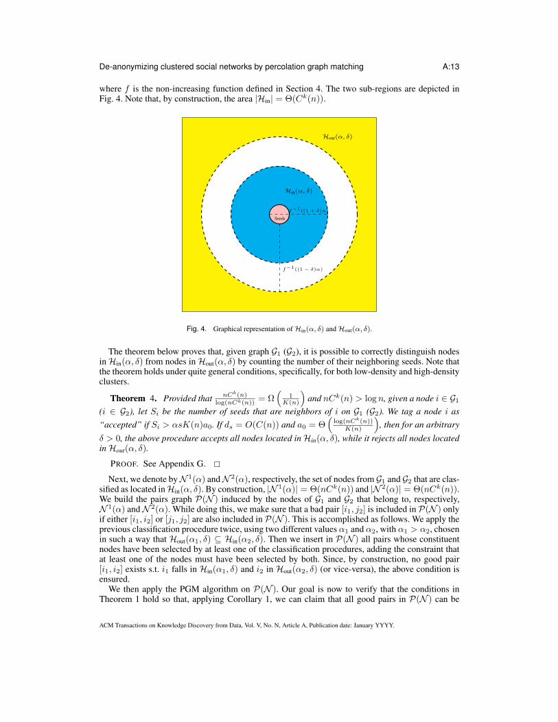
where f is the non-increasing function defined in Section 4. The two sub-regions are depicted inFig. 4. Note that, by construction, the area |Hin| = Θ(Ck(n)).
f−1((1 + δ)α)
Seeds
Hin(α, δ)
Hout(α, δ)
f−1((1 − δ)α)
Fig. 4. Graphical representation of Hin(α, δ) and Hout(α, δ).
The theorem below proves that, given graph G1 (G2), it is possible to correctly distinguish nodesinHin(α, δ) from nodes inHout(α, δ) by counting the number of their neighboring seeds. Note thatthe theorem holds under quite general conditions, specifically, for both low-density and high-densityclusters.
Theorem 4. Provided thatnCk(n)
log(nCk(n))= Ω
(
1K(n)
)
and nCk(n) > log n, given a node i ∈ G1(i ∈ G2), let Si be the number of seeds that are neighbors of i on G1 (G2). We tag a node i as
“accepted” if Si > αsK(n)a0. If ds = O(C(n)) and a0 = Θ(
log(nCk(n))K(n)
)
, then for an arbitrary
δ > 0, the above procedure accepts all nodes located inHin(α, δ), while it rejects all nodes locatedinHout(α, δ).
PROOF. See Appendix G.
Next, we denote byN 1(α) andN 2(α), respectively, the set of nodes from G1 and G2 that are clas-sified as located inHin(α, δ). By construction, |N 1(α)| = Θ(nCk(n)) and |N 2(α)| = Θ(nCk(n)).We build the pairs graph P(N ) induced by the nodes of G1 and G2 that belong to, respectively,N 1(α) andN 2(α). While doing this, we make sure that a bad pair [i1, j2] is included in P(N ) onlyif either [i1, i2] or [j1, j2] are also included in P(N ). This is accomplished as follows. We apply theprevious classification procedure twice, using two different values α1 and α2, with α1 > α2, chosenin such a way that Hout(α1, δ) ⊆ Hin(α2, δ). Then we insert in P(N ) all pairs whose constituentnodes have been selected by at least one of the classification procedures, adding the constraint thatat least one of the nodes must have been selected by both. Since, by construction, no good pair[i1, i2] exists s.t. i1 falls in Hin(α1, δ) and i2 in Hout(α2, δ) (or vice-versa), the above condition isensured.
We then apply the PGM algorithm on P(N ). Our goal is now to verify that the conditions inTheorem 1 hold so that, applying Corollary 1, we can claim that all good pairs in P(N ) can be
ACM Transactions on Knowledge Discovery from Data, Vol. V, No. N, Article A, Publication date: January YYYY.
A:14 C.F. Chiasserini et al.
matched without errors. To this end, let us define m = Θ(nCk(n)), which in order sense equalsthe number of nodes in N 1(α) and N 2(α). Then note that pmin = Θ(pmax), pmax = K(n) and
K(n) = o(m−γ). Thus, for a sufficiently large r = Θ(1) , pmax ≪ m− 3.5r . Since by assumption
nK(n)Ck(n) = Ω(log n), we have mK(n) = Ω(log n) and, hence, mpmin = Ω(log n). It followsthat pmin ≫ m−1. At last, it is easy to see that ao/ac → ∞. Indeed, consider (1) where p isreplaced with pmin, and recall that pmin = Θ(K(n)) and mpmin = Θ(B(n)), then we have:
ac = Θ
(
1
[B(n)]1
r−1K(n)
)
.
I.e., ac = o(1/K(n)) while, by assumption (see Theorem 4),
a0 = Ω
(
log(nCk(n))
K(n)
)
.
In conclusion, we have that all good pairs, whose nodes fall inHin(α1, δ), can be correctly matched.To further expand the set of identified pairs, we pursuit the following simple approach. Starting
from the pairs already matched in the first phase, which act as seeds, we consider a larger region thatincludes the previous one. By properly setting a threshold r, we can match all pairs in this largerregion having at least r neighbors among the seeds. So doing, we successfully match w.h.p. all goodpairs in the region with no errors. More formally, the following theorem allows us to claim that ourapproach can be successfully employed.
Theorem 5. Under the assumption B(n) = Ω(log n), consider a circular region D(0, ρ) ⊆H centered at 0, of radius ρ, with ρ ≥ C(n). Assume that all (or almost all) good pairs whoseconstituent nodes lie within D(0, ρ) have been correctly matched. Then, it is possible to correctlymatch (almost) all good pairs whose constituent nodes are in D(0, ρ1) \ D(0, ρ) with probability1− o(n−1), for ρ1 = ρ+C(n)/2, when K(n) = o([nCk(n)]−γ) for some 0 < γ < 1. In addition,none of the bad pairs formed by nodes in H − D(0, ρ) will be matched, again with probability
1 − o(n−1). This is done by setting threshold r = n2 |D(0, ρ) ∩ D(x, C(n))|K(n)
2 , with |x| = ρ1,and identifying as good pairs those inH \D(0, ρ) that have at least r neighbors among good pairswith vertices in D(0, ρ).
PROOF. The proof is based on the application of standard concentration results, namely, Cher-noff bound and inequalities in Appendix A. The detailed proof is given in [Chiasserini et al.2015a].
Almost all good pairs can be matched w.h.p. by iterating the matching procedure of Theorem 5 anumber of steps equal to Θ(1/C(n)). Indeed, each time the PGM algorithm successfully matches allgood pairs whose constituent nodes lie within distance C(n)/2 from the set of previously matchedpairs. Note that Theorem 5 also guarantees that, jointly over all steps, no bad pair is matched w.h.p.
7.2. Case B(n) = o (log n) and B(n) = ω(n−ξ) ∀ξ > 0 , β > k/2
In this case, since in general nCk(n) is not guaranteed to be greater or equal to log n, we can-not apply Theorem 4. However, given that B(n) = nK(n)Ck(n) = o(log n) and K(n) =o([nCk(n)]−γ) for some 0 < γ < 1, it follows that µ = nCk(n)K2(n) = o(log1−γ n) (under
the assumption β > k/2). Thus we can fix r = Θ(
lognlog logn
)
and apply a standard PGM on the
whole graph GT. In this way, condition (8) holds and w.h.p. no wrong pairs are ever matched at anystage of the algorithm. However, we have to show that, by applying PGM, the process of matchinggood pairs successfully percolates over the all pairs graph. To this end, we need to apply Theorems2 and 3, and, in particular, to show that the conditions in Theorem 3 hold for an opportunely selectedsubgraph of GT, G0.
ACM Transactions on Knowledge Discovery from Data, Vol. V, No. N, Article A, Publication date: January YYYY.

De-anonymizing clustered social networks by percolation graph matching A:15
We then consider the subgraph G0 induced by the m vertices residing in a square box of sideh(n). Observe that, since the percolation process over good pairs is monotonically increasing, thenthe percolation process over G0 is faster than a percolation process over G(m, pmin), where pmin isthe minimum connectivity probability among vertices in G0.
Consider that m = nhk(n) and f(d) = Θ(Cβ(n)h−β(n)), thus
mpmin = nhk(n)K(n)Cβ(n)h−β(n)(a)= Γ(n)r
were Γ(n) is an arbitrarily slow function such that (i) Γ(n) → ∞ and (ii) (a) guarantees that thecondition mpmin ≫ r in Theorem 3 is satisfied. We then derive h(n) as:
h(n) =
(
rΓ(n)
nCβ(n)K(n)
)1
k−β
(10)
where C(n)≪ h(n)≪ 1, by construction. Thus we can successfully apply Theorem 3 by choosinga number of seeds:
a0 = Θ
(
r
pmin
)
= Θ
(
lognlog logn
K(n)Cβ(n)h−β(n)
)
and obtain that PGM successfully matches all good pairs within a distance Θ(h(n)) from the seedset.
To further expand the set of good pairs that are matched, conceptually we can apply again thePGM algorithm by employing all good pairs that have been previously matched as new seed set.Then all good pairs whose constituent nodes lie within a distance Θ(C(n)) from this new seed setwill be matched. Iterating the argument, we can match almost all good pairs in the graph. In practice,however, iterating PGM is not necessary as the matching procedure does never stop until almost allgood pairs in the graph have been matched. This because PGM naturally uses previously matchedpairs as adjoint seeds to match new pairs (when PGM matches a pair and places it in Z(t), it addsone mark to all its neighbors).
The above de-anonymization procedure is summarized in Alg. 2.
Algorithm 2 De-anonymization algorithm used in Section 7.2, 7.3, 7.4, 8.2
Require: G1, G21: if µ = o(n−ξ) then % As in Secs. 7.3-7.42: Set r to an arbitrary constant value
3: else if µ = o(log1−ξ n) then % As in Secs. 7.2-8.24: r ← Θ(log n/ log log n)
5: Select a subregion ofH of size h(n) % As in (10) for Sec. 7.3, (11) for Secs. 7.2-7.46: % and (14) for Sec. 8.2
7: A0 ← seeds inH8: Apply PGM to P(GT) using r and A0 as above9: return Set of matched pairs
7.3. Case B(n) = o(n−ξ) for some 0 < ξ < 1 , β > k/2
This case immediately implies that µ = nCk(n)K2(n) ≪ B(n) = o(n−ξ). Thus condition (9)holds and, for an arbitrarily chosen r = Θ(1) we can again apply a standard PGM on the wholegraph so as to ensure that w.h.p no wrong pairs are ever matched at any stage of the algorithm. Theprocedure reported in Alg. 2 therefore holds also for this case.
ACM Transactions on Knowledge Discovery from Data, Vol. V, No. N, Article A, Publication date: January YYYY.

A:16 C.F. Chiasserini et al.
Specifically, as before we have to show that it is possible to apply Theorems 2 and 3 to an oppor-tune subgraph G0 ⊆ GT. We then consider the subgraph G0 induced by the m vertices residing in asquare box of side h(n). By defining pmin as before, we have again that the matching process overG0 is faster than the matching process over G(m, pmin). However, since r = Θ(1), now we have:
mpmin = nhk(n)K(n)Cβ(n)h−β(n) = Γ(n)
with Γ(n) being an arbitrarily slow function such that Γ(n)→∞ so that condition pmin > m−1 isautomatically satisfied. Deriving h(n), we obtain:
h(n) =
(
Γ(n)
[nCβ(n)K(n)]
)1
k−β
. (11)
Note that condition pmin ≪ m3.5r can be easily met by selecting a sufficiently slow Γ(n). Also,
we have to impose:
a0 = Θ
(
1
(mprmin)1
r−1
)
= Θ
(
1
[nhk(n)]1
r−1 [h−β(n)K(n)Cβ(n)]r
r−1
)
(12)
so as to guarantee a successful matching over G(m, pmin), hence G0, and, by Theorem 2, over thecorresponding subset in GT. Finally, a successful matching of good pairs on GT can be achievedfollowing the same rationale described in Section 7.2.
7.4. Case β ≤ k/2
Since we assume D(n) = Θ(nK(n)Cβ(n)) = O(n1/2−δ) with δ > 0, necessarily we have µ =nC2β(n)K2(n) = O(n−2δ). Thus, again we can properly fix a finite r and apply PGM to matchalmost all good pairs within a range Θ(h(n)) (with h(n) defined as in (11)) under the same conditionon a0 as in (12). (See Alg. 2 for a summary of the procedure to be applied.)
8. HIGH-DENSITY CLUSTERS
We now consider clusters with high graph density, i.e., with K(n) = ω([nCk(n)]−γ) ∀γ > 0. Wefirst focus on the case where β > k/2 and analyze the seed set size that is required for successfulgraph de-anonymation. Specifically, we consider the following two cases:
— Case B(n) = Ω(log1−ξ n), ∀ξ > 0 (Sec. 8.1): a0 = O([maxnCk(n), log n]ǫ), for any ǫ > 0.In this case (large values of B(n)), the graph may have many cliques or quasi-cliques of nodes.Thus, matching nodes using only the local structure of a cluster, may lead to a high number oferrors. For a successful graph de-anonymization we therefore match nodes only on the basis of the‘fingerprint’ provided by their longer edges. In particular, we first trigger the matching procedureusing two sub-regions of side Θ(C(n)), which are sufficiently far from each other and includea suitable number of seeds. To identify the nodes therein, we apply a modified version of PGMalgorithm, which considers only edges spanning between the two sub-regions. Then, by exploitingthe fact that in the high-density cluster regime the distance between two nodes can be estimatedquite precisely, we select a set of compact nodes that are sufficiently far from a matched sub-region, and re-apply the direct matching strategy with a properly chosen r. The procedure can beiterated until almost all nodes are matched.
— B(n) = o(log1−ξ n), for some 0 < ξ < 1 (Sec. 8.2): a0 =
(
log nlog log n
K(n)Cβ(n)h−β(n)
)
. Here the edge
density within a cluster is not very large, thus we safely apply PGM directly on the original pairsgraph, using seeds in an opportunely defined sub-region and by selecting a proper threshold r.
At last (Sec. 8.3), we note that β ≤ k/2 does not represent a meaningful case for high-densityclusters, since it cannot be matched with the above condition on K(n).
ACM Transactions on Knowledge Discovery from Data, Vol. V, No. N, Article A, Publication date: January YYYY.

De-anonymizing clustered social networks by percolation graph matching A:17
8.1. Case B(n) = Ω(log1−ξ n), ∀ξ > 0, and β > k/2
First, observe that B(n) = Ω(log1−ξ n) (for any ξ > 0) implies nCk(n) = Ω(log1−ξ n) ∀ξ >0, given that K(n) ≤ 1. Second, since µ = B(n)K(n), and K(n) = ω([nCk(n)]−γ), ∀γ >0 (or, equivalently K(n) = ω(log−γ n), ∀γ > 0), µ does not meet conditions (8)–(9), and wecannot exploit the corresponding values of r to guarantee a successful matching process. Indeed,as mentioned in Section 5, this case is significantly different from low-density clusters, and thede-anonymization algorithm should disregard all edges whose length is too short (shorter than aproperly defined threshold ω(C(n))) so as to avoid errors (i.e., matching bad pairs).
In order to provide a clear outline of the de-anonymation procedure that we adopt for high-densityclusters, we provide the pseudocode in Algorithm 3. We present the details and prove our analyticalresults in the following sections. In particular, since our approach relies on some results on bipartitegraphs, we introduce them in Sec. 8.1.1. Then we apply such results to our clustered social networkmodel (Sec. 8.1.2), and derive the seed set size that is required to trigger the identification process(Sec. 8.1.3).
Algorithm 3 De-anonymization algorithm used in Section 8.1
Require: G1, G2, A0, ǫ > 01: Identify two squared regions,H1,H2 ⊂ H, of side h(n) = Ω(C(n)) and g(n) = ω(C(n))
apart from each other, including a0 = O([maxnCk(n), log n]ǫ) seeds each2: r ← 4/ǫ3: Build the pairs graph P(H12) induced by nodes inH1 andH2
4: Apply PGM to P(H12) using r as above and only inter-region edges % Trigger phase5: while No. of newly matched pairs > 0 do % Expansion phase6: H2 ← compact set of nodes sufficiently apart fromH1 and within Θ(C(n)) from each other7: Build the pairs graph P(H12) induced by nodes inH1 andH2
8: Update r as in Theorem 7 and use matched nodes inH1 as seeds9: Consider inter-region edges only and match all pairs in P(H12), whose constituent nodes lie in
H2, with at least r already-matched neighboring pairs, whose constituent nodes lie inH1
10: return Set of matched pairs
8.1.1. Results on bipartite graphs. Let GT be an m1 ×m2 bipartite graph. LetM1 denote the setof vertices on the left hand side (LHS), with |M1| = m1, andM2 the set of vertices on the righthand side (RHS), with |M2| = m2. We assume that for any pair of vertices i ∈ M1 and j ∈ M2
an edge (i, j) exists in the graph with probability pij , with pmin ≤ pij ≤ pmax and pmax = ηpmin
for some constant η > 1. Our goal is to identify the required number of seeds a0 located in eitherside of the graph, i.e., with a0 = |Al
0| inM1 and a0 = |Ar0| inM2, such that vertices inM1 and
M2 can be correctly matched.Let us first consider the case where m1 = m2 = m, for which the theorem below holds.
Theorem 6. Assume that GT is an m ×m bipartite graph and that two sets of seeds, Al0 and
Ar0, both of cardinality a0 > ac, are available on, respectively, the LHS and the RHS of the graph.
Then the PGM algorithm with threshold r ≥ 4 correctly identifies m − o(m) good pairs w.h.p.on the RHS and the LHS of graph P(GT), with no errors, under the same four conditions listed inTheorem 1.
PROOF. See Appendix H.
Theorem 6 can be extended to the general case where m1 6= m2, as stated in the corollary below.
Corollary 2. Assume that GT is an m1 ×m2 bipartite graph and define m = min(m1,m2).Under the same assumptions of Theorem 6, the PGM algorithm with threshold r ≥ 4 successfully
ACM Transactions on Knowledge Discovery from Data, Vol. V, No. N, Article A, Publication date: January YYYY.

A:18 C.F. Chiasserini et al.
identifies w.h.p. m − o(m) good pairs on both the LHS and the RHS of P(GT), with no errors.
Furthermore, the PGM algorithm can be successfully applied to a pairs graph P(GT) ⊂ P(GT)comprising a finite fraction of pairs on both the LHS and the RHS of P(GT) and satisfying the
following constraint: a bad pair [i1, j2] ∈ P(GT) is included in P(GT) only if either [i1, i2] or
[j1, j2] are also in P(GT).
PROOF. The assertion can be proved by following the same arguments as in Theorem 6 andapplying Corollary 1.
Finally, we prove the following result, which shows that all good pairs can be matched with noerrors w.h.p.
Theorem 7. Consider that GT is an m1 ×m2 bipartite graph with m1 = ω(√m2) and that a
seed setAl0 is available on the LHS of the graph, with |Al
0| = a0 = Θ(m1). With probability larger
than 1 − e− m1√
m2 , all the m2 good pairs on the RHS can be successfully identified with no errors,provided that:
(1) 1√m2≪ pmin ≤ pmax ≪ 1
(2) pmin = Θ(pmax)(3) a matching algorithm is used on P(GT) that matches all pairs on the RHS that have at least r
adjacent seeds on the LHS, with r = a0pmin
2 .
The same result holds in case of pairs graph comprising a finite fraction of all possible pairs on theRHS.
PROOF. Without loss of generality, we assume a0 ≥ cm2 for some c > 0. First, observe that,given a good pair [j1, j2] on the RHS of the pairs graph, the number of its adjacent seeds on the LHSis E[Ng] ≥ a0pmin = 2r. Thus, by applying concentration results in App. A and union bound, wehave:
P(all good pairs on the RHS have at least r adjacent seeds) ≥ 1−m2e−cm1pminH( 1
2 )
≥ 1− e− m1√
m2
which imply that all good pairs on the RHS are successfully matched since m1 = ω(√m2). Sim-
ilarly, considering a bad pair [j1, k2] on the RHS, the number of its adjacent seeds on the LHS isE[Nb] ≤ cm2(pmax)
2 ≪ r. Thus, by applying concentration results in App. A and union bound,we have:
P(all bad pairs on the RHS have less than r adjacent seeds) ≥ 1−m22e
−cm1pmin
4 log(
pmin(pmax)2
)
≥ 1− e− m1√
m2 .
8.1.2. The de-anonymization procedure. We now outline how our proposed matching algorithmfor high-density clusters works. We start by focusing on single vertices in H so as to identify re-gions in H where PGM can be successfully applied. Specifically, we consider two hyper-cubicregions, H1,H2 ⊂ H, whose side is h(n) = Ω(C(n)) and whose distance is g(n) = ω(C(n))(see Fig. 3). Note that, by construction, given two vertices i ∈ H1 and j ∈ H2, pmin =K(n)f(g(n) +
√kh(n)) ≤ pij ≤ K(n)f(g(n)) = pmax. Let us assume pmax = ηpmin for
some constant η > 1.We then extract vertices in H1 and H2 from the rest of vertices so that we can focus on the
bipartite graph induced by the nodes in the two sub-regions, along with the edges between them.To this end, we assume that two sufficiently large sets of seeds are available in H1 and H2 so
ACM Transactions on Knowledge Discovery from Data, Vol. V, No. N, Article A, Publication date: January YYYY.
De-anonymizing clustered social networks by percolation graph matching A:19
that Theorem 4 given in Section 7.1 can be applied (or Corollary 4 given in Appendix E when
Ck(n) = o(
lognn
)
).
At this point, we consider the pairs graph originated from the above bipartite graph. In this regard,observe that we can use the same procedure as in Section 7, to make sure that a bad pair [i1, j2] isincluded in the pair graph only if either [i1, i2] or [j1, j2] are also included in it. We can then applyCorollary 2.
It follows that the execution of the PGM algorithm ensures that almost all of the good pairsin either the LHS or the RHS of the pairs graph are correctly de-anonymized. Without lack ofgenerality, we assume that almost all pairs on LHS are de-anonymized, i.e., m1 < m2, and thata non-negligible fraction of the good pairs on the RHS have still to be identified. Then the rest ofgood pairs on the RHS can be matched by applying Theorem 7.
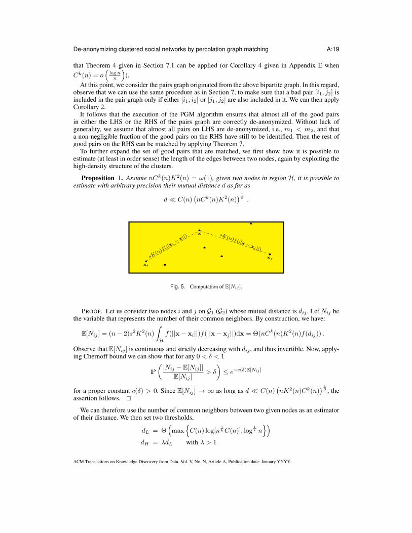
To further expand the set of good pairs that are matched, we first show how it is possible toestimate (at least in order sense) the length of the edges between two nodes, again by exploiting thehigh-density structure of the clusters.
Proposition 1. Assume nCk(n)K2(n) = ω(1), given two nodes in region H, it is possible toestimate with arbitrary precision their mutual distance d as far as
d≪ C(n)(
nCk(n)K2(n))
1β .
xi
xj
x
sK(n)f(||x
i− x
||) sK(n)f(||x−xj ||)
Fig. 5. Computation of E[Nij ].
PROOF. Let us consider two nodes i and j on G1 (G2) whose mutual distance is dij . Let Nij bethe variable that represents the number of their common neighbors. By construction, we have:
E[Nij ] = (n− 2)s2K2(n)
∫
Hf(||x− xi||)f(||x− xj ||)dx = Θ(nCk(n)K2(n)f(dij)) .
Observe that E[Nij ] is continuous and strictly decreasing with dij , and thus invertible. Now, apply-ing Chernoff bound we can show that for any 0 < δ < 1
P
( |Nij − E[Nij ]|E[Nij ]
> δ
)
≤ e−c(δ)E[Nij ]
for a proper constant c(δ) > 0. Since E[Nij ] → ∞ as long as d ≪ C(n)(
nK2(n)Ck(n))
1β , the
assertion follows.
We can therefore use the number of common neighbors between two given nodes as an estimatorof their distance. We then set two thresholds,
dL = Θ(
max
C(n) log[n1kC(n)], log
1k n)
dH = λdL with λ > 1
ACM Transactions on Knowledge Discovery from Data, Vol. V, No. N, Article A, Publication date: January YYYY.

A:20 C.F. Chiasserini et al.
and we leverage the above result to correctly classify the edges going out of previously matchednodes into three categories: edges that are shorter than dL, edges that are longer than dH and edgesof length comprised between dL and dH . In particular, we are interested in the latter, for which thefollowing result holds.
Proposition 2. Assume K(n) = ω([nCk(n)]−γ) ∀γ > 0, and nCk(n) = Ω(log1−ξn) ∀ξ > 0.Consider a set comprising a finite fraction of the nodes in G1 (G2) lying in a region of side Θ(C(n)),and the edges incident to them. For an arbitrarily selected δ > 0, w.h.p (i.e., with a probabilitylarger than 1 − [C(n)]k) we can select all edges whose length d is (1 + δ)dL ≤ d ≤ (1 − δ)dH .Furthermore, no edges whose length d < (1− δ)dL and d > (1 + δ)dH are selected.
The proof follows the same lines as the proof in Appendix G (see [Chiasserini et al. 2015a] forfurther details).
At this point, we consider a bipartite graph whose LHS is still represented by H1, and whoseRHS is given by the nodes that are connected with those in H1 through edges of length comprisedbetween dL and dH . Again, we consider the pairs graph originated from them and apply Theorem7 so as to match w.h.p. all good pairs on the RHS, with no errors. The procedure is then iterated soas to successfully de-anonymize the entire network. Note that, at every step we apply the followingproposition to extract a group of matched nodes whose mutual distance is Θ(C(n)).
Proposition 3. Assume K(n) = ω([nCk(n)]−γ) ∀γ > 0 and nCk(n) = Ω(log1−ξn), ∀ξ > 0.Given a node i, we can set a threshold dT = Θ(C(n)) and select all nodes in G1 (G2) whoseestimated distance from i is less than dT . So doing, for an arbitrarily selected δ > 0, we successfullyselect with a probability larger than 1 − [C(n)]k all nodes whose real distance is d ≤ (1 − δ)dT .Furthermore, no nodes whose distance from i is d > (1 + δ)dT are selected by our algorithm.
The proof is similar to that of Proposition 2 (see also [Chiasserini et al. 2015a]).
8.1.3. Seed set size. To explicitly derive the required seed set size, we need to further specifyh(n) and g(n), which are to be carefully selected so as to minimize the resulting critical size ac inTheorem 6 and Corollary 2.
First, recalling (1) and Theorem 1, we have:
ac =
(
1− 1
r
)(
(r − 1)!
m(pmins2)r
)1
r−1
≤(
r − 1
(mpmins2)1
r−1 pmins2
)
≤ r
pmins2. (13)
Thus, ac can be minimized by maximizing pmin, i.e., by minimizing g(n) (recall that pmin =
K(n)f(g(n) +√kh(n))). However, g(n) and h(n) must also be selected in such a way that condi-
tion 1) of Theorem 6 is met. Additionally, as mentioned, it must be ensured that h(n) = Ω(C(n)).At last, by standard concentration results, m1 and m2 turn out to be both Θ(nhk(n)) provided that
h(n) ≥ (log n/n)1/k.Previous considerations suggest to fix:
h(n) = Θ(maxC(n), (log n/n)1/k) ≥ (log n/n)1/k
(i.e., the minimum possible value in order sense), which corresponds to having m =Θ(maxnCk(n), log n) (recall that m = min(m1,m2)). We then derive g(n) by forcing pmax ≈m−α
r , with 3.5 < α < 4 and r ≥ 4. Note that condition 1) of Theorem 6 is met since pmax andpmin are both Θ(m−α
r ). Hence, we have:
pmax = Θ([maxnCk(n), log n]−αr )
g(n) = Θ(
C(n)[maxnCk(n), log n]αβ [K(n)]1β
)
Given the above expression for pmax, considering that pmax = ηpmin and using (13), the seedset size can be made as small as a0 = O([maxnCk(n), log n]ǫ), for any ǫ > 0, by choosing
ACM Transactions on Knowledge Discovery from Data, Vol. V, No. N, Article A, Publication date: January YYYY.

De-anonymizing clustered social networks by percolation graph matching A:21
r > 4ǫ . Finally, we remark that the obtained a0 is in order sense greater than the number of seeds
needed to apply Theorem 4 while selecting nodes in regionsH1 anH2, thus the whole constructionis consistent.
8.2. Case B(n) = o(log1−ξ n), for some 0 < ξ < 1, and β > k/2
First, we observe that B(n) = o(log1−ξ n) implies nCk(n) = o(log1−ξ n). On its turn, this implies
β < k so as to guarantee that D(n) = Ω(logn). In this case, µ = o(log1−ξ n), thus we can select ras in (8) and apply the PGM directly on the pairs graph P(GT), without worrying about errors. Thesame procedure outlined in Alg. 2 holds in this case.
The idea is to show that PGM successfully matches almost all good pairs on an opportune bipartitesubgraph of GT. To show this, we have to extend Theorem 3 to bipartite graphs, as done in Corollary3.
Corollary 3. Consider a subgraph of GT(V, E) denoted by G0(V0, E0), which is an m1 ×m2
bipartite graph with m1 = Θ(m2). Assume that, for any pair of vertices i ∈ M1 and j ∈ M2, anedge (i, j) exists in the graph with probability pij , with pmin ≤ pij ≤ pmax and pmax = ηpmin forsome constant η > 1.
Under (8), applying the PGM algorithm to P(GT) (with r = Θ( lognlog log n )) guarantees that
m− o(m) good pairs are matched with no errors, if a0 randomly chosen seeds among verticesinM1 and inM2 are available, provided that
(1) m1 →∞;(2) m1pmin ≫ r;(3) a0 = Θ( r
pmin) .
PROOF. The proof follows the same lines as the proof of Theorem 3.
It follows that we can trigger percolation on GT, whenever we can find two boxes of side h(n)separated by g(n) so that the induced bipartite graph satisfies the assumptions of Corollary 3, i.e.,we place a sufficiently large number of seeds a0 in each of the boxes.
In particular, we select:
h(n) = g(n) ≥ max [C(n), log n/n] (14)
obtaining m1 = Θ(nhk(n)), m2 = Θ(m1) and
pmin = Θ(K(n)Cβ(n)h−β(n))
pmax = Θ(pmin)
Now, to satisfy condition 2 of Corollary 3, we must impose m1pmin ≫ r. By following the samesteps as in Section 7.2, we obtain a condition on the number of seeds a0 to be placed in each box:
a0 =
(
lognlog logn
K(n)Cβ(n)h−β(n)
)
.
Note that Corollary 3 ensures that, after the execution of PGM, almost all nodes in the boxesof side h(n) are correctly identified. Similarly to the procedure reported in Section 7.2, to ensurethat we can further expand the set of identified nodes, we can invoke Theorems 2 and 7 by settingh(n) = g(n).
8.3. Case β ≤ k/2
This case is impossible. Indeed the assumptions i) β ≤ k2 and ii) K(n) = ω([nCK(n)]−γ) for every
γ > 0 contrast with the assumption that D(n) = O(n12−δ) for some δ > 0. Indeed, by i) and ii) and
given that C(n) = Ω(n− 1k ), we have D(n) = Θ(nK(n)Cβ(n)) = Ω(nK(n)n− 1
2 ) = ω(n12−δ).
ACM Transactions on Knowledge Discovery from Data, Vol. V, No. N, Article A, Publication date: January YYYY.

A:22 C.F. Chiasserini et al.
Table II. Main results on seed set size for sample cases of low-density and high-density clusters and fordifferent conditions on B(n) and β/k
Scenario
Low-densityConditions
B(n) = nζ−α B(n) = Θ(1) B(n) = o(nζ−α)
β ≥ k/2 k/2 < β < k(
ζ < α < 1 − β 1−ζk
)
∧ β < k
K(n) = n−α, α > 0 Required seed set size
Θ(nα logn) ω
(
nα[
log nlog log n
] kk−β
)
nα(1+r)−2
r−1+
β(1−ζ)k−β
High-densityConditions
B(n) = nζ B(n) = 1 β ≤ k/2ζ > 0 ∧ β > k/2 k/2 < β < k
K(n) = 1 Required seed set size
nǫ, ∀ǫ > 0 ω(
log nlog log n
)1+β
k−β Impossible
9. EXPERIMENTAL VALIDATION
A summary of our analytical results obtained when K(n) = n−α and B(n) = nζ−α (α, ζ ≥ 0)is reported in Table II. The table highlights the trend of the required seed set size, in some specialcases that will be explored in our experimental validation. Although our results hold asymptoticallyas n → ∞, we can expect to qualitatively observe the main effects predicted by the analysis alsoin finite-size graphs. We will first investigate the performance of graph matching algorithms insynthetic graphs generated according to our model of clustered networks, allowing us to assess thevalidity of our results for the different considered regimes. Next, we consider real social networkgraphs, exploring also variants and improvements of matching algorithms.
9.1. Synthetic graphs
In this section we consider bi-dimensional graphs having n = 10, 000, the sampling probability s =0.8 and, unless otherwise specified, the average node degree in the ground-truth graph D(n) = 30.
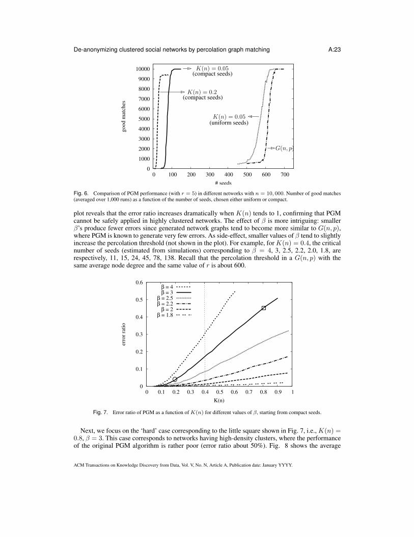
Fig. 6 reports the average number of correctly matched nodes across 1, 000 runs of the PGMalgorithm (using r = 5) in various cases, as function of the number of seeds. In each run, seedsare either chosen uniformly at random among all nodes (label ‘uniform seeds’), or as a compact setaround one randomly chosen seed (label ‘compact seeds’). In our model of clustered graphs, wehave fixed β = 3 (the decay exponent of the edge probability beyond C(n)), and we consider eitherK(n) = 0.05 or K(n) = 0.2. As reference, in the plot we also show the phase transition occurring(at about 600 seeds) when GT is a G(n, p) graph having the same average node degree. The plotconfirms the wave-like nature of the identification process as predicted by our analysis, namely: i)clustered networks (larger K(n)) can be matched starting from a much smaller seed set as comparedto G(n, p); ii) such huge reduction requires seeds to be selected within a small sub-region ofH.
What the plot in Fig. 6 does not clearly show (except for a rough estimate based on the maximumnumber of correctly matched nodes) is the error ratio incurred by the PGM algorithm, which isexpected to become larger and larger as we increase the level of clustering in the network. Thisphenomenon is confirmed by Fig. 7, which reports the average error ratio (bad matches over allmatches) incurred by PGM as a function of K(n), starting from a compact set of seeds. In Fig. 7we have considered also different values of β. The little circle denotes the operating point alreadyconsidered for the left-most curve in Fig. 6 (K(n) = 0.2), having an error ratio of about 5%. The
ACM Transactions on Knowledge Discovery from Data, Vol. V, No. N, Article A, Publication date: January YYYY.
De-anonymizing clustered social networks by percolation graph matching A:23
0
1000
2000
3000
4000
5000
6000
7000
8000
9000
10000
0 100 200 300 400 500 600 700
good m
atch
es
# seeds
(uniform seeds)
(compact seeds)
(compact seeds)
K(n) = 0.05
G(n, p)
K(n) = 0.05
K(n) = 0.2
Fig. 6. Comparison of PGM performance (with r = 5) in different networks with n = 10, 000. Number of good matches(averaged over 1,000 runs) as a function of the number of seeds, chosen either uniform or compact.
plot reveals that the error ratio increases dramatically when K(n) tends to 1, confirming that PGMcannot be safely applied in highly clustered networks. The effect of β is more intriguing: smallerβ’s produce fewer errors since generated network graphs tend to become more similar to G(n, p),where PGM is known to generate very few errors. As side-effect, smaller values of β tend to slightlyincrease the percolation threshold (not shown in the plot). For example, for K(n) = 0.4, the criticalnumber of seeds (estimated from simulations) corresponding to β = 4, 3, 2.5, 2.2, 2.0, 1.8, arerespectively, 11, 15, 24, 45, 78, 138. Recall that the percolation threshold in a G(n, p) with thesame average node degree and the same value of r is about 600.
0
0.1
0.2
0.3
0.4
0.5
0.6
0 0.1 0.2 0.3 0.4 0.5 0.6 0.7 0.8 0.9 1
err
or
rati
o
K(n)
β = 4β = 3
β = 2.5β = 2.2
β = 2β = 1.8
Fig. 7. Error ratio of PGM as a function of K(n) for different values of β, starting from compact seeds.
Next, we focus on the ‘hard’ case corresponding to the little square shown in Fig. 7, i.e., K(n) =0.8, β = 3. This case corresponds to networks having high-density clusters, where the performanceof the original PGM algorithm is rather poor (error ratio about 50%). Fig. 8 shows the average
ACM Transactions on Knowledge Discovery from Data, Vol. V, No. N, Article A, Publication date: January YYYY.
A:24 C.F. Chiasserini et al.
1
10
100
1000
10000
10 20 30 40 50 60 70 80 90 100
aver
age
num
ber
of
mat
ched
nodes
# seeds
PGM - good matches - r = 7PGM - bad matches - r = 7f = 1, r = 5 - good matches
f = 1, r = 5 - bad matches 1
10
100
1000
10000
10 20 30 40 50 60 70 80 90 100
aver
age
num
ber
of
mat
ched
nodes
# seeds
f = 1, r = 4 - good matchesf = 1, r = 4 - bad matches
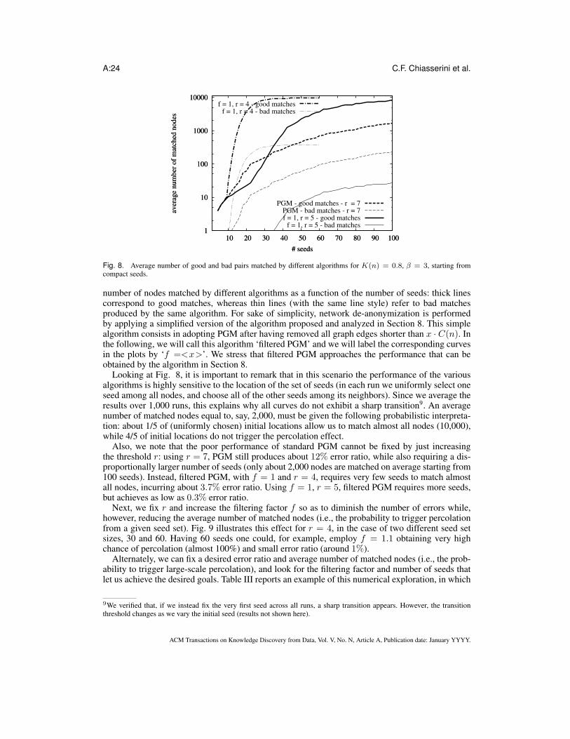
Fig. 8. Average number of good and bad pairs matched by different algorithms for K(n) = 0.8, β = 3, starting fromcompact seeds.
number of nodes matched by different algorithms as a function of the number of seeds: thick linescorrespond to good matches, whereas thin lines (with the same line style) refer to bad matchesproduced by the same algorithm. For sake of simplicity, network de-anonymization is performedby applying a simplified version of the algorithm proposed and analyzed in Section 8. This simplealgorithm consists in adopting PGM after having removed all graph edges shorter than x · C(n). Inthe following, we will call this algorithm ‘filtered PGM’ and we will label the corresponding curvesin the plots by ‘f =<x>’. We stress that filtered PGM approaches the performance that can beobtained by the algorithm in Section 8.
Looking at Fig. 8, it is important to remark that in this scenario the performance of the variousalgorithms is highly sensitive to the location of the set of seeds (in each run we uniformly select oneseed among all nodes, and choose all of the other seeds among its neighbors). Since we average theresults over 1,000 runs, this explains why all curves do not exhibit a sharp transition9. An averagenumber of matched nodes equal to, say, 2,000, must be given the following probabilistic interpreta-tion: about 1/5 of (uniformly chosen) initial locations allow us to match almost all nodes (10,000),while 4/5 of initial locations do not trigger the percolation effect.
Also, we note that the poor performance of standard PGM cannot be fixed by just increasingthe threshold r: using r = 7, PGM still produces about 12% error ratio, while also requiring a dis-proportionally larger number of seeds (only about 2,000 nodes are matched on average starting from100 seeds). Instead, filtered PGM, with f = 1 and r = 4, requires very few seeds to match almostall nodes, incurring about 3.7% error ratio. Using f = 1, r = 5, filtered PGM requires more seeds,but achieves as low as 0.3% error ratio.
Next, we fix r and increase the filtering factor f so as to diminish the number of errors while,however, reducing the average number of matched nodes (i.e., the probability to trigger percolationfrom a given seed set). Fig. 9 illustrates this effect for r = 4, in the case of two different seed setsizes, 30 and 60. Having 60 seeds one could, for example, employ f = 1.1 obtaining very highchance of percolation (almost 100%) and small error ratio (around 1%).
Alternately, we can fix a desired error ratio and average number of matched nodes (i.e., the prob-ability to trigger large-scale percolation), and look for the filtering factor and number of seeds thatlet us achieve the desired goals. Table III reports an example of this numerical exploration, in which
9We verified that, if we instead fix the very first seed across all runs, a sharp transition appears. However, the transitionthreshold changes as we vary the initial seed (results not shown here).
ACM Transactions on Knowledge Discovery from Data, Vol. V, No. N, Article A, Publication date: January YYYY.
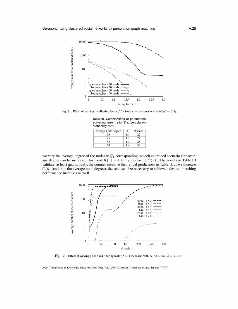
De-anonymizing clustered social networks by percolation graph matching A:25
1
10
100
1000
10000
1 1.05 1.1 1.15 1.2 1.25 1.3
aver
age
num
ber
of
mat
ched
nodes
filtering factor, f
good matches - 30 seedsbad matches - 30 seeds
good matches - 60 seedsbad matches - 60 seeds
Fig. 9. Effect of varying the filtering factor f for fixed r = 4 (scenario with K(n) = 0.8).
Table III. Combinations of parametersachieving error ratio 3%, percolationprobability 50%
average node degree f # seeds36 1.1 2245 1.2 2453 1.3 2864 1.4 32
we vary the average degree of the nodes in GT corresponding to each examined scenario (the aver-age degree can be increased, for fixed K(n) = 0.8, by increasing C(n)). The results in Table IIIvalidate, at least qualitatively, the counter-intuitive theoretical predictions in Table II: as we increaseC(n) (and thus the average node degree), the seed set size necessary to achieve a desired matchingperformance increases as well.
1
10
100
1000
10000
0 50 100 150 200 250 300
aver
age
num
ber
of
mat
ched
nodes
# seeds
good - r = 3bad - r = 3
good - r = 4bad - r = 4
good - r = 5bad - r = 5
Fig. 10. Effect of varying r for fixed filtering factor f = 1 (scenario with K(n) = 0.5, β = k = 4).
ACM Transactions on Knowledge Discovery from Data, Vol. V, No. N, Article A, Publication date: January YYYY.
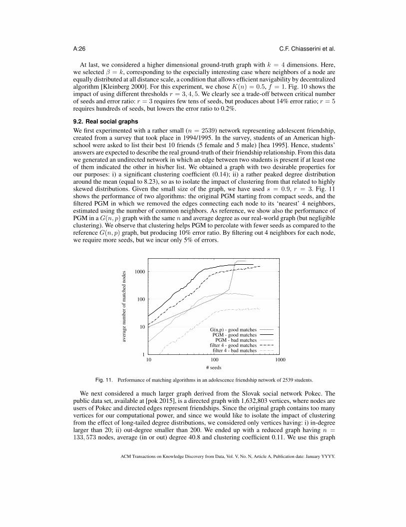
A:26 C.F. Chiasserini et al.
At last, we considered a higher dimensional ground-truth graph with k = 4 dimensions. Here,we selected β = k, corresponding to the especially interesting case where neighbors of a node areequally distributed at all distance scale, a condition that allows efficient navigability by decentralizedalgorithm [Kleinberg 2000]. For this experiment, we chose K(n) = 0.5, f = 1. Fig. 10 shows theimpact of using different thresholds r = 3, 4, 5. We clearly see a trade-off between critical numberof seeds and error ratio: r = 3 requires few tens of seeds, but produces about 14% error ratio; r = 5requires hundreds of seeds, but lowers the error ratio to 0.2%.
9.2. Real social graphs
We first experimented with a rather small (n = 2539) network representing adolescent friendship,created from a survey that took place in 1994/1995. In the survey, students of an American high-school were asked to list their best 10 friends (5 female and 5 male) [hea 1995]. Hence, students’answers are expected to describe the real ground-truth of their friendship relationship. From this datawe generated an undirected network in which an edge between two students is present if at least oneof them indicated the other in his/her list. We obtained a graph with two desirable properties forour purposes: i) a significant clustering coefficient (0.14); ii) a rather peaked degree distributionaround the mean (equal to 8.23), so as to isolate the impact of clustering from that related to highlyskewed distributions. Given the small size of the graph, we have used s = 0.9, r = 3. Fig. 11shows the performance of two algorithms: the original PGM starting from compact seeds, and thefiltered PGM in which we removed the edges connecting each node to its ‘nearest’ 4 neighbors,estimated using the number of common neighbors. As reference, we show also the performance ofPGM in a G(n, p) graph with the same n and average degree as our real-world graph (but negligibleclustering). We observe that clustering helps PGM to percolate with fewer seeds as compared to thereference G(n, p) graph, but producing 10% error ratio. By filtering out 4 neighbors for each node,we require more seeds, but we incur only 5% of errors.
1
10
100
1000
10 100 1000
aver
age
num
ber
of
mat
ched
nodes
# seeds
G(n,p) - good matchesPGM - good matches
PGM - bad matchesfilter 4 - good matches
filter 4 - bad matches
Fig. 11. Performance of matching algorithms in an adolescence friendship network of 2539 students.
We next considered a much larger graph derived from the Slovak social network Pokec. Thepublic data set, available at [pok 2015], is a directed graph with 1,632,803 vertices, where nodes areusers of Pokec and directed edges represent friendships. Since the original graph contains too manyvertices for our computational power, and since we would like to isolate the impact of clusteringfrom the effect of long-tailed degree distributions, we considered only vertices having: i) in-degreelarger than 20; ii) out-degree smaller than 200. We ended up with a reduced graph having n =133, 573 nodes, average (in or out) degree 40.8 and clustering coefficient 0.11. We use this graph
ACM Transactions on Knowledge Discovery from Data, Vol. V, No. N, Article A, Publication date: January YYYY.
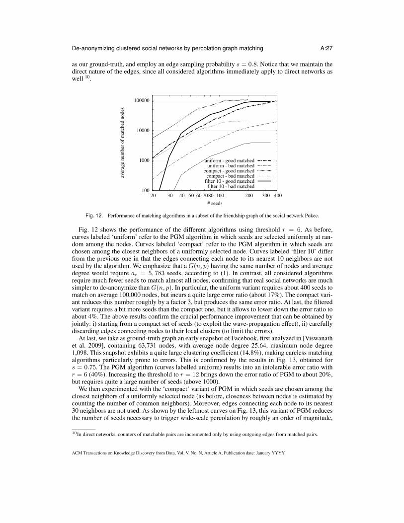
De-anonymizing clustered social networks by percolation graph matching A:27
as our ground-truth, and employ an edge sampling probability s = 0.8. Notice that we maintain thedirect nature of the edges, since all considered algorithms immediately apply to direct networks aswell 10.
100
1000
10000
100000
20 30 40 50 60 70 80 100 200 300 400
aver
age
num
ber
of
mat
ched
nodes
# seeds
uniform - good matcheduniform - bad matched
compact - good matchedcompact - bad matched
filter 10 - good matchedfilter 10 - bad matched
Fig. 12. Performance of matching algorithms in a subset of the friendship graph of the social network Pokec.
Fig. 12 shows the performance of the different algorithms using threshold r = 6. As before,curves labeled ‘uniform’ refer to the PGM algorithm in which seeds are selected uniformly at ran-dom among the nodes. Curves labeled ‘compact’ refer to the PGM algorithm in which seeds arechosen among the closest neighbors of a uniformly selected node. Curves labeled ‘filter 10’ differfrom the previous one in that the edges connecting each node to its nearest 10 neighbors are notused by the algorithm. We emphasize that a G(n, p) having the same number of nodes and averagedegree would require ac = 5, 783 seeds, according to (1). In contrast, all considered algorithmsrequire much fewer seeds to match almost all nodes, confirming that real social networks are muchsimpler to de-anonymize than G(n, p). In particular, the uniform variant requires about 400 seeds tomatch on average 100,000 nodes, but incurs a quite large error ratio (about 17%). The compact vari-ant reduces this number roughly by a factor 3, but produces the same error ratio. At last, the filteredvariant requires a bit more seeds than the compact one, but it allows to lower down the error ratio toabout 4%. The above results confirm the crucial performance improvement that can be obtained byjointly: i) starting from a compact set of seeds (to exploit the wave-propagation effect), ii) carefullydiscarding edges connecting nodes to their local clusters (to limit the errors).
At last, we take as ground-truth graph an early snapshot of Facebook, first analyzed in [Viswanathet al. 2009], containing 63,731 nodes, with average node degree 25.64, maximum node degree1,098. This snapshot exhibits a quite large clustering coefficient (14.8%), making careless matchingalgorithms particularly prone to errors. This is confirmed by the results in Fig. 13, obtained fors = 0.75. The PGM algorithm (curves labelled uniform) results into an intolerable error ratio withr = 6 (40%). Increasing the threshold to r = 12 brings down the error ratio of PGM to about 20%,but requires quite a large number of seeds (above 1000).
We then experimented with the ‘compact’ variant of PGM in which seeds are chosen among theclosest neighbors of a uniformly selected node (as before, closeness between nodes is estimated bycounting the number of common neighbors). Moreover, edges connecting each node to its nearest30 neighbors are not used. As shown by the leftmost curves on Fig. 13, this variant of PGM reducesthe number of seeds necessary to trigger wide-scale percolation by roughly an order of magnitude,
10In direct networks, counters of matchable pairs are incremented only by using outgoing edges from matched pairs.
ACM Transactions on Knowledge Discovery from Data, Vol. V, No. N, Article A, Publication date: January YYYY.
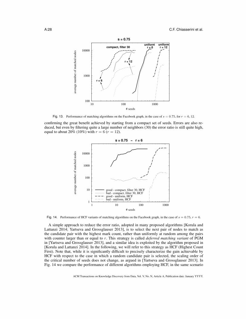
A:28 C.F. Chiasserini et al.
100
1000
10000
10 100 1000
aver
age
nu
mb
er o
f m
atch
ed n
od
es
# seeds
r = 6 r = 12
r = 6
r = 12
compact, filter 30uniform uniform
s = 0.75
Fig. 13. Performance of matching algorithms on the Facebook graph, in the case of s = 0.75, for r = 6, 12.
confirming the great benefit achieved by starting from a compact set of seeds. Errors are also re-duced, but even by filtering quite a large number of neighbors (30) the error ratio is still quite high,equal to about 20% (10%) with r = 6 (r = 12).
1
10
100
1000
10000
1 10 100 1000
aver
age
nu
mb
er o
f m
atch
ed n
od
es
# seeds
good - compact, filter 30, HCFbad - compact, filter 30, HCFgood - uniform, HCFbad - uniform, HCF
s = 0.75 − r = 6
Fig. 14. Performance of HCF variants of matching algorithms on the Facebook graph, in the case of s = 0.75, r = 6.
A simple approach to reduce the error ratio, adopted in many proposed algorithms [Korula andLattanzi 2014; Yartseva and Grossglauser 2013], is to select the next pair of nodes to match asthe candidate pair with the highest mark count, rather than uniformly at random among the pairswith counter larger than or equal to r. This strategy is called deferred matching variant of PGMin [Yartseva and Grossglauser 2013], and a similar idea is exploited by the algorithm proposed in[Korula and Lattanzi 2014]. In the following, we will refer to this strategy as HCF (Highest CountFirst). Note that, while it is significantly difficult to precisely characterize the gain achievable byHCF with respect to the case in which a random candidate pair is selected, the scaling order ofthe critical number of seeds does not change, as argued in [Yartseva and Grossglauser 2013]. InFig. 14 we compare the performance of different algorithms employing HCF, in the same scenario
ACM Transactions on Knowledge Discovery from Data, Vol. V, No. N, Article A, Publication date: January YYYY.
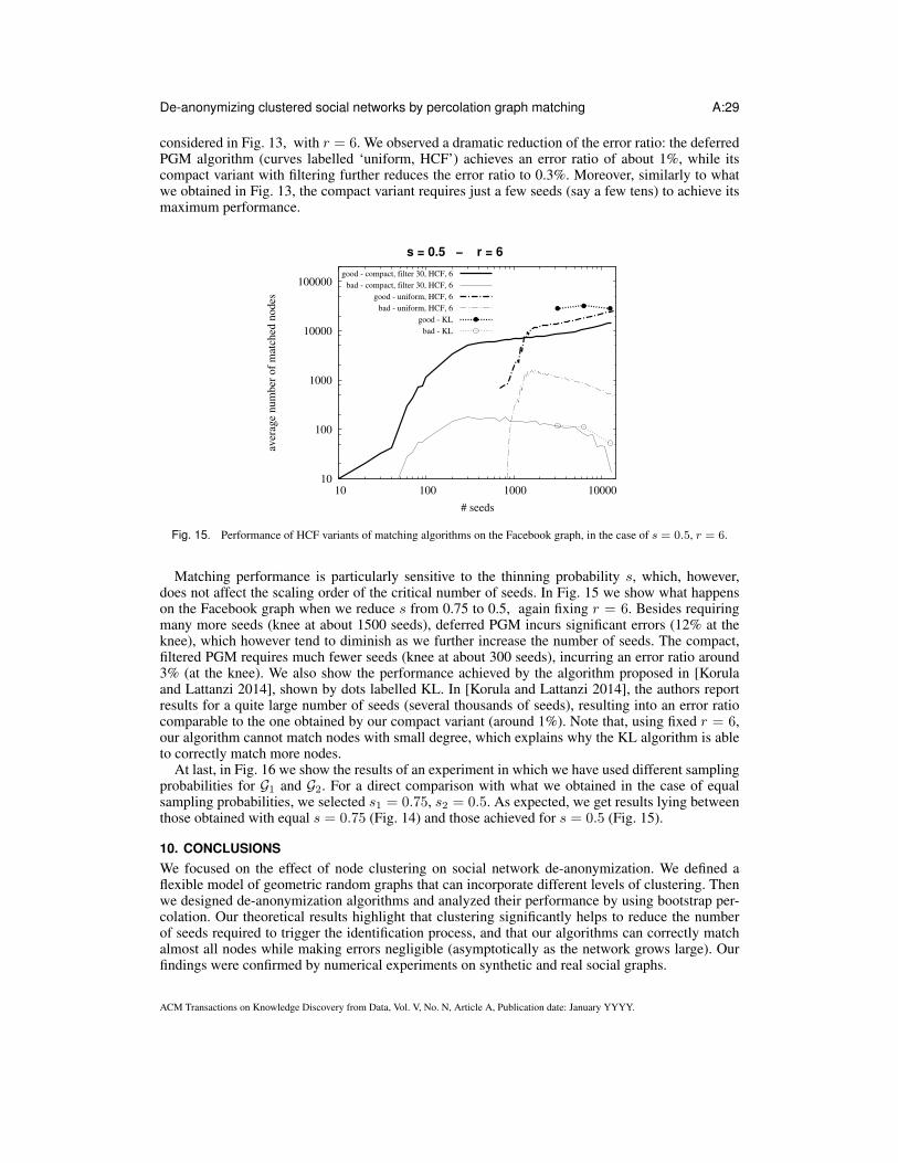
De-anonymizing clustered social networks by percolation graph matching A:29
considered in Fig. 13, with r = 6. We observed a dramatic reduction of the error ratio: the deferredPGM algorithm (curves labelled ‘uniform, HCF’) achieves an error ratio of about 1%, while itscompact variant with filtering further reduces the error ratio to 0.3%. Moreover, similarly to whatwe obtained in Fig. 13, the compact variant requires just a few seeds (say a few tens) to achieve itsmaximum performance.
10
100
1000
10000
100000
10 100 1000 10000
aver
age
nu
mb
er o
f m
atch
ed n
od
es
# seeds
good - compact, filter 30, HCF, 6
bad - compact, filter 30, HCF, 6
good - uniform, HCF, 6
bad - uniform, HCF, 6
good - KL
bad - KL
s = 0.5 − r = 6
Fig. 15. Performance of HCF variants of matching algorithms on the Facebook graph, in the case of s = 0.5, r = 6.
Matching performance is particularly sensitive to the thinning probability s, which, however,does not affect the scaling order of the critical number of seeds. In Fig. 15 we show what happenson the Facebook graph when we reduce s from 0.75 to 0.5, again fixing r = 6. Besides requiringmany more seeds (knee at about 1500 seeds), deferred PGM incurs significant errors (12% at theknee), which however tend to diminish as we further increase the number of seeds. The compact,filtered PGM requires much fewer seeds (knee at about 300 seeds), incurring an error ratio around3% (at the knee). We also show the performance achieved by the algorithm proposed in [Korulaand Lattanzi 2014], shown by dots labelled KL. In [Korula and Lattanzi 2014], the authors reportresults for a quite large number of seeds (several thousands of seeds), resulting into an error ratiocomparable to the one obtained by our compact variant (around 1%). Note that, using fixed r = 6,our algorithm cannot match nodes with small degree, which explains why the KL algorithm is ableto correctly match more nodes.
At last, in Fig. 16 we show the results of an experiment in which we have used different samplingprobabilities for G1 and G2. For a direct comparison with what we obtained in the case of equalsampling probabilities, we selected s1 = 0.75, s2 = 0.5. As expected, we get results lying betweenthose obtained with equal s = 0.75 (Fig. 14) and those achieved for s = 0.5 (Fig. 15).
10. CONCLUSIONS
We focused on the effect of node clustering on social network de-anonymization. We defined aflexible model of geometric random graphs that can incorporate different levels of clustering. Thenwe designed de-anonymization algorithms and analyzed their performance by using bootstrap per-colation. Our theoretical results highlight that clustering significantly helps to reduce the numberof seeds required to trigger the identification process, and that our algorithms can correctly matchalmost all nodes while making errors negligible (asymptotically as the network grows large). Ourfindings were confirmed by numerical experiments on synthetic and real social graphs.
ACM Transactions on Knowledge Discovery from Data, Vol. V, No. N, Article A, Publication date: January YYYY.

A:30 C.F. Chiasserini et al.
1
10
100
1000
10000
1 10 100 1000
aver
age
nu
mb
er o
f m
atch
ed n
od
es
# seeds
good - compact, filter 30, HCF
bad - compact, filter 30, HCF
good - uniform, HCF
bad - uniform, HCF
r = 6
Fig. 16. Performance of HCF variants of matching algorithms on the Facebook graph, in the case of s1 = 0.75, s2 = 0.5,r = 6.
Our work can be extended along several directions, including the effect of erroneously selectedseeds, more general graph models and partially overlapping node sets, as done in [Kazemi et al.2015a; Kazemi et al. 2015b] for Erdos–Renyi graphs.
APPENDIX
A. DEVIATION BOUNDS FOR THE BINOMIAL DISTRIBUTION
In this paper we frequently use some classical deviation bounds for the binomial distribution (seee.g. Lemma 1.1 p. 16 in [Penrose 2003]), which we report here for the reader’s convenience. Definethe function H(x) := 1 − x + x log x, for x > 0. Suppose n ∈ N, p ∈ (0, 1) and 0 < k < n. Letµ = np. If k ≥ µ then
P (Bin(n, p) ≥ k) ≤ exp
(
−µH(
k
µ
))
(15)
and if k ≤ µ then
P (Bin(n, p) ≤ k) ≤ exp
(
−µH(
k
µ
))
. (16)
Finally, if k ≥ e2µ then
P (Bin(n, p) ≥ k) ≤ exp
(
−(
k
2
)
log
(
k
µ
))
. (17)
B. CLUSTERING COEFFICIENT
We focus on a single vertex, which, for the sake of simplicity, is assumed to be placed at the originof regionH. Then, we compute the average number of its neighbor pairs that are connected, i.e.,
T (n) =(n− 1)(n− 2)
2K3(n)
∫ ∫
f(||x1||)f(||x2||) · f(||x2 − x1||) dx1 dx2 .
The clustering coefficient is then given by2T (n)
D(n)(D(n)−1) .
ACM Transactions on Knowledge Discovery from Data, Vol. V, No. N, Article A, Publication date: January YYYY.

De-anonymizing clustered social networks by percolation graph matching A:31
T (n) can be evaluated as follows11:
T (n) ∼ n2K3(n)
∫ ∫
||x1||<||x2||f(||x1||)f(||x2||) · f(||x2 − x1||) dx1 dx2 .
To compute (in order sense) the above integral, we partition the integral domain in two regionsdistinguishing the following two cases: i) ||x1 − x2|| ≥ δ||x2|| for an arbitrarily chosen δ > 0 andii) the complementary case ||x1 − x2|| < δ||x2||. In the first case, by triangular inequality we haveδ||x2|| ≤ ||x1 − x2|| ≤ ||x2|| + ||x1|| ≤ 2||x2||, and thus f(||x2 − x1||) is in order sense equal tof(||x2||) over the considered domain. As a consequence, for the integral over the first region, weget:
T1(n) ∼ n2K3(n)
∫ ∫
||x1||<||x2||||x1−x2||>δ||x2||
f2(||x2||)f(||x1||) dx1 dx2
∼ n2K3(n)
∫ 1
0
ρk−12 max
(
1,
(
C(n)
ρ2
)−2β)
∫ ρ2
0
ρk−11 max
(
1,
(
C(n)
ρ1
)−β)
dρ1 dρ2 .
It is easy to see that a similar expression is obtained when the integral extends over the domainfor which ||x2 − x1|| < δ||x2||. In particular, considering that in this case f(||x1||) ∼ f(||x2||) byconstruction, and denoting with ρ3 = ||x1 − x2||, we have:
T2(n) ∼ n2K3(n)
∫ 1
0
ρk−12 f2(||ρ2||)
∫ δρ2
0
f(||ρ3||) dρ1 dρ3
In conclusion, we obtain:
T (n) = T1(n) + T2(n) =
Θ(
n2K3(n)C(n)2k)
β > 2k3
Θ(
n2K3(n)C(n)2k log 1C(n)
)
β = 2k3
Θ(
n2K3(n)C(n)3β)
β < 2k3 .
Recalling (4), for β > k the clustering coefficient turns out to be Θ(K(n)). Similarly, for β =
k, it is Θ(
K(n)log2[1/C(n)]
)
. For 2k3 < β < k, it is Θ
(
K(n)C(n)2(k−β))
, while for β = 2k3 it is
Θ(
K(n)C(n)β log[1/C(n)])
. Finally, for β < 2k3 , the clustering coefficient is Θ
(
K(n)C(n)β)
.
C. PROOF OF THEOREM 1
The theorem assumes pmin ≫ m−1. In Theorem 2 in [Chiasserini et al. 2016], we considered
the case pmin ≫√m−3/r−1, with r ≥ 4. Here, instead, we consider the complementary case
pmin = O(√
m−3/r−1)
. With reference to PGM algorithm reported in Algorithm 4, we define:
— Bt(GT) as the set of pairs in P(GT) that at time step t have already collected a least r marks. It iscomposed of good pairs B′t(GT) and bad pairs B′′t (GT);
—At(GT) as the set of matchable pairs at time t. Similarly to Bt(GT), it comprises good pairsA′t(GT)
and bad pairs A′′t (GT). In general, At(GT) and Bt(GT) do not coincide as Bt(GT) may include
conflicting pairs that are not present in At(GT);—Zt(GT) as the set of pairs that have been matched up to time t. By construction, |Zt| = t, ∀t.
Next, we define
TGpmin= mint s.t. |At(G(m, pmin)| = t; TGpmax
= mint s.t. |At(G(m, pmax)| = t
11Given f and g, f ∼ g denotes that f = Θ(g)
ACM Transactions on Knowledge Discovery from Data, Vol. V, No. N, Article A, Publication date: January YYYY.

A:32 C.F. Chiasserini et al.
Algorithm 4 The PGM algorithm
1: A0 = B0 = A0(n), Z0 = ∅, t = 02: while At \ Zt 6= ∅ do3: t = t+ 14: Randomly select a pair [∗1, ∗2] ∈ At−1\Zt−1 and add one mark to all neighbor pairs of [∗1, ∗2]
inM(GT).5: Let ∆Bt be the set of all neighbor pairs of [∗1, ∗2] inM(GT) whose mark counter has reached
threshold r at time t.
6: Construct set ∆At ⊆ ∆Bt as follows. Order the pairs in ∆Bt in an arbitrary way, select themsequentially and test them for inclusion in ∆At:
7: if the selected pair in ∆Bt has no conflicting pair in At−1 or ∆At then8: Insert the pair in ∆At
9: else10: Discard it11: Zt=Zt−1∪[∗1, ∗2], Bt=Bt−1∪∆Bt, At=At−1∪∆At
12: return T = t, ZT = AT
By Lemma 3.1, we have that both TGpminand TGpmax
are equal to m− o(m). Then inductively on
t, ∀t < min(TGpmin, TGpmax
), w.h.p.:
|B′′t (GT )| ≤ |B′′t ((G(m, pmax))| = ∅ . (18)
In (18), the inequality descends by monotonicity of sets B′′t with respect to “≤st”. The followingequality descends from Corollary 1 in [Chiasserini et al. 2016] applied to Gpmax
. We remark that,under our assumption on pmin and pmax, we have t0 = T in Corollary 1 in [Chiasserini et al. 2016],along with:
|At(GT )|(a)= |B′t(GT )|
(b)
≥ |B′t(G(m, pmin))|(c)= |At(G(m, pmin))|
(d)> t. (19)
In (19), equality (a) is an immediate consequence of (18), inequality (b) holds by monotonicity ofsets B′t with respect to “≤st”, while equality (c) descends from Lemma 3.1. Inequality (d) descendsfrom the fact that we assume t < TGpmin
.
Thus, necessarily, AT (GT ) = T ≥ min(TGpmin, TGpmax
) = m− o(m) and B′′T (GT ) = ∅.
D. PROOF OF COROLLARY 1
Essentially the scheme of Theorem 1 can be repeated to show that there exists t1 < T such that
Bt1(P) comprises all good pairs in P and no bad pairs. First observe that P can always be trans-formed intoP(G′′T ), being G′′T a proper subgraph of G′T (and therefore of GT), by adding and removingonly bad pairs.
Second, from Theorem 1 we know that, denoted by N the number of vertices in G′′T , for a t1 =(N)−3/r−ǫ
(pmins)2= o(N), it holds: B′t1(P(G′′T )) = N (equal, by construction, to the number of good pairs
in P). Third, again from Theorem 1, it holds that B′′t1(P(G′′T )) = ∅.Hence, if we prove that B′′t1(P) = ∅, we can conclude that B′t1(P) = N since condition
B′′t1(P(G′′T )) = ∅ necessarily implies B′t(P(G′′T )) = B′t(P) for every t ≤ t1. Indeed, by construction,
the subgraphs of P(G′′T ) and P induced by their good pairs are identical.
To prove that B′′t1(P) = ∅, we can upper-bound the number of marks collected at time t by
every bad pair [i1, j2] ∈ P with a binomial r.v. Bi(t, p2maxs2) and, then, proceed exactly as in the
proof of Corollary 1 in [Chiasserini et al. 2016] to show that PB′′t1(P) 6= ∅ → 0. Given that, by
ACM Transactions on Knowledge Discovery from Data, Vol. V, No. N, Article A, Publication date: January YYYY.

De-anonymizing clustered social networks by percolation graph matching A:33
construction, a bad pair [i1, j2] can be included in P only if either [i1, i2] or [j1, j2] are also in P ,
then, none of the bad pairs in P can be matched for t > t1, because it will be necessarily blockedby a previously matched good pair.
E. PROOF OF THEOREM 2 AND COROLLARY 4
First we assume that PGM G0(V0, E0) successfully matches all good pairs. Consider the evolutionof PGM over GT(V, E) and G0(V0, E0). Since (8) holds we can assume that no bad pairs reach thethreshold at any stage of the process, and restrict our analysis to good pairs. With abuse of notationwe say that a good pair belongs to V0 if the corresponding vertex belongs to V0.
First, observe that if we assume that at time t ZGT(t) = ZG0(t), necessarilyAG0(t) = AGT
(t)∩V0and, thus, |AGT
(t)| ≥ |AG0(t)| > 0. However, in general, we cannot assume ZGT(t) = ZG0(t) at
every t. Indeed, PGM operating over GT can select and match at some point some good pairs notbelonging to V0, which have already reached the threshold, while the PGM operating over V0 cannot.We conclude that in general ZGT
(t) 6= ZG0(t).
Let us consider t ≤ |V0|. Since |ZGT(t)| ≤ |ZG0
(t)| = t by construction, necessarily ZG0(t) \
ZGT(t) 6= ∅. Let τ = mint′≤t zG0
(t′)) 6∈ ZGT(t). Note that zG0
(τ) must be in AG0(τ − 1) and thus
also inAGT(t)∪ZGT
(t). Indeed, since by construction ZG0(τ − 1) ⊂ ZGT
(t), we have ZG0(τ − 1)∪
AG0(τ − 1) ⊆ ZGT
(t) ∪ AGT(t). This implies that zG0
(τ) ∈ AGT(t), i.e., AGT
(t) 6= ∅. By inductionover t, we can then prove that AGT
(t) 6= ∅ for any t ≤ V0, hence TGT≥ |V0|. Now, consider
t > |V0|. Since ZG0(t) = ZG0
(TG0) = V0 by construction, we have that either V0 ⊆ ZGT
(t) or,necessarily, ZG0
(t) \ ZGT(t) 6= ∅. In the latter case, we can repeat the previous argument to show
that AGT(t) 6= ∅. It follows that V0 ⊆ ZGT
(TGT). The extension to the more general case in which
PGM over G0(V0, E0) matches almost all good pairs, can be proved along the same lines.A more general version of the previous theorem is given below for the case where the threshold
α is a function of n.
Corollary 4. Assume that a target distance D(n) ≫ C(n) can be found, with D(n) ≥(
lognn
)1k
, satisfying the following condition:
nDk(n) = Ω
(
log(nDk(n))
K(n)f(D(n))
)
.
Given a node i ∈ G1 (i ∈ G2), let Si be the number of seeds that are neighbors of i on G1 (G2).We say that node i is tagged as “accepted” if Si > f(D(n))sK(n)a0. If ds = O(D(n)) and
a0 = Θ(
log[nDk(n)]K(n)f(D(n))
)
, then, for an arbitrary δ > 0, the above procedure accepts all nodes located
inHin(f(D(n)), δ), while it rejects all nodes located inHout(f(D(n), δ).
PROOF. The proof follows exactly the same lines as the proof of Theorem 4.
Note that, in the above statement sK(n) is the probability that a node in G1 (G2) is connected with aseed node at distance C(n) or shorter. Thus, αsK(n)a0 provides a suitable threshold for the numberof connections between a node and the a0 seed vertices.
F. PROOF OF THEOREM 3
Assume that r = lognlog logn , i.e., (8) holds. This implies that we can disregard bad pairs and the graph
de-anonymization process corresponds to a pure bootstrap percolation process on the subgraph ofP(GT) induced by good pairs.
Also, it is straightforward to see that the percolation probability over a graph is monotonicallyincreasing with respect to the graph ordering relation “≤st” (see Section 3 for the ordering relationdefinition). This because at every t we have A(t) = A′(t) = B′(t), in light of (8), and B′(t) is
ACM Transactions on Knowledge Discovery from Data, Vol. V, No. N, Article A, Publication date: January YYYY.

A:34 C.F. Chiasserini et al.
obliviously monotonic with respect to ≤st. Thus, since by construction G(m, pmin) ≤st G0, ifpercolation successfully occurs on G(m, pmin), then it takes place successfully also over G0.
To prove that the matching process is successful on G(m, pmin), we follow an approach similarto that in [Janson et al. 2012]. Consider the evolution of At; it is clear that percolation stops whenA(t) becomes empty. Since A(t) includes the seed set, clearly it cannot be empty till t = a0. Then,recalling that a0 > r
pmins2(1 + δ), we should consider t > r
pmins2(1 + δ).
We first observe that the probability that a good pair has a number of matched neighbors greater
than or equal to r at time t is Bin(t, pmins2). For t1 = ⌈ r(1+δ)
pmins2⌉,
P(
Bin(t1, pmins2) ≥ r
)
≥ 2c
with c being a suitable small positive constant. This holds because the expectation of the Binomial
is by construction equal to ⌈ r(1+δ)pmins2
⌉pmins2 > r. Thus, using concentration results in App. A, we
can easily show that w.h.p. A(t1) > cn, hence A(t) > A(t1) > cn ≥ t ∀t ∈ [t1, cn]. Now,consider t ∈ [cn, n (1− e−r)] and define t2 = ⌊cn⌋. Observe that, given our choice of r, we haven (1− e−r) = n− o(n). Moreover, applying again inequalities in App. A, we have:
P(
Bin(t2, pmins2) < r
)
≤ exp
(
−t2pmins2H
(
r
t2pmins2
))
≤ exp
(
−t2pmins2
[
1− δ
2
])
where H(b) = 1 − b + b log b. The above probability tends to 0 faster (in order sense) than
e−r. It follows that E[n − A(t)] ≤ E[n − A(t2)] < e−t2pmins2(1−δ), thus, by Markov inequal-
ity n−A(t) ≤ n−A(t2) < ne−r w.h.p. In conclusion, w.h.p. the percolation process does notstop for t ∈ [cn, n (1− e−r)].
G. PROOF OF THEOREM 4
Without loss of generality, let us focus on G1 and consider a node i ∈ Hin(α, δ). By construction,the number of seeds that are neighbors of i on G1 is given by Si =
∑
σ∈A0XiσS
1iσ ≥st Yi ≥st Y
where
Yi = Bin(a0, sK(n)f(maxσ∈A0
||xi − xσ||))
and Y = Bin(a0, sK(n)(1+δ)α), with E[Y ] = sK(n)(1+δ)αa0. Now, using inequalities in App.A, we can bound:
P (Yi < αsK(n)a0) ≤ exp
(
−E[Yi]H(αsK(n)a0
E[Yi]
)
)
≤ exp
(
−(1 + δ)αsK(n)a0H( 1
1 + δ
)
)
(20)
with H(b) = 1− b+ b log b.If we consider jointly all nodes inHin(α, δ) and we denote with Nin their number, we can bound
the probability that every node inHin(α, δ) is accepted:
P (all nodes inHin are accepted | Nin) ≤ 1−Nin exp
(
−(1 + δ)αsK(n)a0H( 1
1 + δ
)
)
, (21)
with (21) that tends to 1 if logNin − (1 + δ)αsH(
11+δ
)
K(n)a0 → −∞. This can be en-
forced by opportunely setting a0 = Ω(
logNin
K(n)
)
. Since by construction |Hin| > Ck(n) ≥ lognn ,
we have w.h.p. Nin ≤ 2n|Hin| by standard concentration results in App. A. As a consequence,
P (all vertices inHin are accepted)→ 1 provided that a0 = Ω(
log[nCk(n)]K(n)
)
.
ACM Transactions on Knowledge Discovery from Data, Vol. V, No. N, Article A, Publication date: January YYYY.
De-anonymizing clustered social networks by percolation graph matching A:35
Then we focus on the nodes in Hout(α, δ) and we show that all those nodes are jointly rejected.Conceptually we repeat the same approach as before, however, the argument is made slightly morecomplex by the fact that, in order to obtain tight bounds on the probability that all nodes inHout(α, δ)are jointly rejected, we need to partitionHout(α, δ) into smaller sub-regions containing nodes whichlie at similar distance from the seeds.
Assuming δ < e2−1e2 , we define H1
out = H1(α, e2−1e2 ) ⊂ Hout(α, δ) and H0
out(α, δ) =
Hout(α, δ) \ H1out. Furthermore, we partition H1
out into disjoint sub-regions, i.e., H1out = ∪h≥1H1,h
out ,
with H1,hout = Hout(
α,hβe2−1hβe2
) \ Hout(α,(h+1)βe2−1(h+1)βe2
). Now, given a vertex i in H0out (H1,h
out ), the
number of its neighbor seeds Si on G1 can be bounded from above by a Bin(a0, sK(n)(1 − δ)α)(
Bin(a0,sK(n)hβe2
α))
. Furthermore, by elementary geometrical arguments, it can be shown that: i)
|H0out| = Θ(Ck(n)), ii) |H1,1
out | = Θ(Ck(n)) and iii)H1,hout = Θ(hk−1H1,1
out ).
Denoted with N0out and N1,h
out the number of nodes in H0out and H1,h
out , respectively, by exploitingagain inequalities in App. A, w.h.p. we have:
P(
all nodes inH0out are rejected
)
≤ 1 − N0out exp
(
−(1− δ)αsK(n)a0H(
1− δ))
→ 1 .
The above expression holds under the assumption that a0 = Ω(
log[nCk(n)]K(n)
)
. Indeed, we remark
that N0out ≤ 2n|H0
out| = Θ(nCk(n)) w.h.p. At last,
P(
all nodes inH1out are rejected
)
≤ 1−∞∑
h=1
N1,hout exp
(
−αsK(n)a02
[β log h+ 2]
)
.
For every h, N1,hout ≤ 2n|H1,h| = Θ(nhk−1Ck(n)); also, the number of sub-regions of H1
out is
O(n/Ck(n)). Thus, w.h.p. we have that jointly on all h’s, the number of nodes in these sub-regions
can be bounded by 2n|H1,h|. Under the assumption that a0 = Ω(
log[nCk(n)]K(n)
)
, it can be easily
shown that P(
all nodes inH1out are rejected
)
→ 1.
H. PROOF OF THEOREM 6
For any two vertices i ∈M1 and j ∈M2, let Xij be the Bernoulli random variable that representsthe presence of an edge (i, j) ∈ E . By construction, Ber(pmin) ≤st Xij ≤st Ber(pmax). I.e., two
variables Xij and Xij , with distribution, respectively, Ber(pmin) and Ber(pmax), can be defined on
the same probability space as Xij such that Xij ≤ Xij ≤ Xij point-wise.
We consider the corresponding pairs graph P(GT), which is, by construction, composed of all thepairs of vertices residing inM1 andM2 and of the edges connecting pairs of vertices inM1 withpairs of vertices in M2. We denote by P1 and P2, respectively, the set of pairs of P(GT), whosevertices lie inM1 andM2. Observe that, given two good pairs [i1, i2] ∈ P1 and [j1, j2] ∈ P2, thepresence of an edge in P(GT) is associated with the random variable:
Y[i1,i2],[j1,j2] = XijXijS1ijS
2ij = X2
ijS1ijS
2ij
where S1ij and S2
ij are mutually independent Ber(s) r.v’s, which are in turn independent of Xij .
By construction, pmins2 ≤ E[Y[i1,i2],[j1,j2]] ≤ pmaxs
2. Instead, given two bad pairs [i1, k2] ∈ P1
and [j1, l2] ∈ P2, Y[i1,k2],[j1,l2] = XijXklS1ijS
2kl, with p2mins
2 ≤ E[Y[i1,k2],[j1,l2]] ≤ p2maxs2.
Finally, if we consider one good pair and one bad pair (e.g., [i1, i2] ∈ P1 and [j1, k2] ∈ P2),Y[i1,i2],[j1,k2] = XijXikS
1ijS
2ik, with p2mins
2 ≤ E[Y[i1,i2],[j1,j2]] ≤ p2maxs2.
Recall that we assume that two seed sets, Al0 ∈ P1 and Ar
0 ∈ P2 (with |Al0| = |Ar
0|), are avail-able. On P(GT) we run the PGM algorithm [Yartseva and Grossglauser 2013], opportunely modi-
ACM Transactions on Knowledge Discovery from Data, Vol. V, No. N, Article A, Publication date: January YYYY.
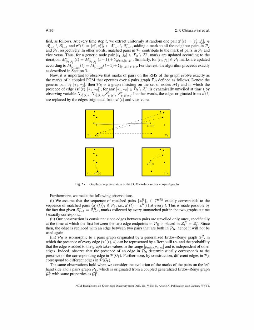
A:36 C.F. Chiasserini et al.
fied, as follows. At every time step t, we extract uniformly at random one pair zl(t) = [zl1, zl2]t ∈
Alt−1 \ Z l
t−1 and zr(t) = [zr1 , z
r2 ]t ∈ Ar
t−1 \ Zrt−1, adding a mark to all the neighbor pairs in P2
and P1, respectively. In other words, matched pairs in P1 contribute to the mark of pairs in P2 andvice versa. Thus, for a generic node pair [i1, j2] ∈ P2 \ Zr
t , marks are updated according to theiteration: Mr
[i1,j2](t) = Mr
[i1,j1](t− 1)+ Y
zl(t),[i1,j2]. Similarly, for [i1, j2] ∈ P1 marks are updated
according to M l[i1,j2]
(t) = M l[i1,j2]
(t−1)+Y[i1,j2],zr(t). For the rest, the algorithm proceeds exactly
as described in Section 3.Now, it is important to observe that marks of pairs on the RHS of the graph evolve exactly as
the marks of a coupled PGM that operates over a pairs graph PR defined as follows. Denote thegeneric pair by [∗1, ∗2]; then PR is a graph insisting on the set of nodes M2 and in which thepresence of edge (zr(t), [∗1, ∗2]), for any [∗1, ∗2] ∈ P2 \ Zr
t , is dynamically unveiled at time t byobserving variable Xzl
1(t)∗1Xzl
2(t)∗2Slzl1(t)∗1
Srzl1(t)∗2
. In other words, the edges originated from zl(t)
are replaced by the edges originated from zr(t) and vice-versa.
zl(t)
zr(t)
zL(t)
zR(t)
PL PR
P1 P2
Fig. 17. Graphical representation of the PGM evolution over coupled graphs.
Furthermore, we make the following observations.
(i) We assume that the sequence of matched pairs zRt t ∈ P(R) exactly corresponds to thesequence of matched pairs zr(t)t ∈ P2, i.e., zr(t) = z
R(t) at every t. This is made possible bythe fact that given Zr
t−1 = ZRt−1, marks collected by every unmatched pair in the two graphs at time
t exactly correspond.(ii) Our construction is consistent since edges between pairs are unveiled only once, specifically
at the time at which the first between the two edge endpoints in PR is placed in ZRt = Zr
t . Sincethen, the edge is replaced with an edge between two pairs that are both in PR, hence it will not beused again.
(iii) PR is isomorphic to a pairs graph originated by a generalized Erdos–Renyi graph GRT , inwhich the presence of every edge (zr(t), ∗) can be represented by a Bernoulli r.v. and the probabilitythat the edge is added to the graph takes values in the range [pmin, pmax] and is independent of otheredges. Indeed, observe that the presence of an edge in PR deterministically corresponds to thepresence of the corresponding edge in P(GT). Furthermore, by construction, different edges in PR
correspond to different edges in P(GT).The same observations hold when we consider the evolution of the marks of the pairs on the left
hand side and a pairs graph PL, which is originated from a coupled generalized Erdos–Renyi graphGLT with same properties as GRT .
ACM Transactions on Knowledge Discovery from Data, Vol. V, No. N, Article A, Publication date: January YYYY.

De-anonymizing clustered social networks by percolation graph matching A:37
Now, clearly G(m, pmin) ≤st GRT ≤st G(m, pmax) and G(m, pmin) ≤st GLT ≤st G(m, pmax),i.e., GRT (GLT ) can be obtained by opportunely thinning a graph G(m, pmax), while a graph
G(m, pmin) can be obtained by opportunely thinning GRT (GLT ). Then we invoke Theorem 1 to con-
clude our proof and show that our algorithm correctly percolates over GRT and GLT and, thus, overthe bipartite graph GT.
REFERENCES
1995. Add health public data set, wave I (online). (1995). http://www.cpc.unc.edu/projects/addhealth
2015. Pokec network dataset – KONECT. (May 2015). http://konect.uni-koblenz.de/networks/soc-pokec-relationships
Fabian Abel, Nicola Henze, Eelco Herder, and Daniel Krause. 2010. Interweaving Public User Profiles on the Web. InProceedings of the 18th International Conference on User Modeling, Adaptation, and Personalization (UMAP’10).Springer-Verlag, Berlin, Heidelberg, 16–27. DOI:http://dx.doi.org/10.1007/978-3-642-13470-8 4
Lars Backstrom, Cynthia Dwork, and Jon Kleinberg. 2007. Wherefore Art Thou R3579x?: Anonymized Social Networks,Hidden Patterns, and Structural Steganography. In Proceedings of the 16th International Conference on World Wide
Web (WWW ’07). ACM, New York, NY, USA, 181–190. DOI:http://dx.doi.org/10.1145/1242572.1242598
Karl Bringmann, Tobias Friedrich, and Anton Krohmer. 2014. Algorithms - ESA 2014: 22th Annual European Symposium,
Wroclaw, Poland, September 8-10, 2014. Proceedings. Springer Berlin Heidelberg, Berlin, Heidelberg, Chapter De-anonymization of Heterogeneous Random Graphs in Quasilinear Time, 197–208.
Carla-Fabiana Chiasserini, Michele Garetto, and Emilio Leonardi. 2015a. Companion technical report. Technical Report.https://www.dropbox.com/s/4ddvmgy0zkauj0d/TechRep.pdf?dl=0
Carla-Fabiana Chiasserini, Michele Garetto, and Emilio Leonardi. 2015b. Impact of Clustering on the Performance of Net-work De-anonymization. In Proceedings of the 2015 ACM on Conference on Online Social Networks (COSN ’15).ACM, New York, NY, USA, 83–94. DOI:http://dx.doi.org/10.1145/2817946.2817953
C. F. Chiasserini, M. Garetto, and E. Leonardi. 2016. Social Network De-Anonymization Under Scale-Free User Relations.IEEE/ACM Transactions on Networking in press (2016).
A. Egozi, Y. Keller, and H. Guterman. 2013. A Probabilistic Approach to Spectral Graph Matching. IEEE Transactions on
Pattern Analysis and Machine Intelligence 35, 1 (2013), 18–27. DOI:http://dx.doi.org/10.1109/TPAMI.2012.51
Keith Henderson, Brian Gallagher, Lei Li, Leman Akoglu, Tina Eliassi-Rad, Hanghang Tong, and Christos Faloutsos. 2011.It’s Who You Know: Graph Mining Using Recursive Structural Features. In Proceedings of the 17th ACM SIGKDD
International Conference on Knowledge Discovery and Data Mining (KDD ’11). ACM, New York, NY, USA, 663–671. DOI:http://dx.doi.org/10.1145/2020408.2020512
Svante Janson, Tomasz Łuczak, Tatyana Turova, and Thomas Vallier. 2012. Bootstrap percolation on the random graphGn,p. Ann. Appl. Probab. 22, 5 (10 2012), 1989–2047. DOI:http://dx.doi.org/10.1214/11-AAP822
S. Ji, W. Li, N. Z. Gong, P. Mittal, and R. Beyah. 2016. Seed-Based De-Anonymizability Quantification of Social Networks.IEEE Transactions on Information Forensics and Security 11, 7 (July 2016), 1398–1411.
Shouling Ji, Weiqing Li, Mudhakar Srivatsa, and Raheem Beyah. 2014. Structural Data De-anonymization: Quantification,Practice, and Implications. In Proceedings of the 2014 ACM SIGSAC Conference on Computer and Communications
Security (CCS ’14). ACM, New York, NY, USA, 1040–1053.
Ehsan Kazemi, S. Hamed Hassani, and Matthias Grossglauser. 2015a. Growing a Graph Matching from a Handful of Seeds.Proc. VLDB Endow. 8, 10 (June 2015), 1010–1021. DOI:http://dx.doi.org/10.14778/2794367.2794371
E. Kazemi, L. Yartseva, and M. Grossglauser. 2015b. When can two unlabeled networks be aligned under partial over-lap?. In 2015 53rd Annual Allerton Conference on Communication, Control, and Computing (Allerton). 33–42.DOI:http://dx.doi.org/10.1109/ALLERTON.2015.7446983
Jon Kleinberg. 2000. The Small-world Phenomenon: An Algorithmic Perspective. In Proceedings of the Thirty-
second Annual ACM Symposium on Theory of Computing (STOC ’00). ACM, New York, NY, USA, 163–170.DOI:http://dx.doi.org/10.1145/335305.335325
Nitish Korula and Silvio Lattanzi. 2014. An Efficient Reconciliation Algorithm for Social Networks. Proc. VLDB Endow. 7,5 (Jan. 2014), 377–388. DOI:http://dx.doi.org/10.14778/2732269.2732274
M. Leordeanu and M. Hebert. 2005. A spectral technique for correspondence problems using pairwise constraints. In Tenth
IEEE International Conference on Computer Vision (ICCV’05) Volume 1, Vol. 2. 1482–1489 Vol. 2.
Jure Leskovec, Jon Kleinberg, and Christos Faloutsos. 2007. Graph Evolution: Densification and Shrinking Diameters. ACM
Trans. Knowl. Discov. Data 1, 1, Article 2 (March 2007). DOI:http://dx.doi.org/10.1145/1217299.1217301
S. Melnik, H. Garcia-Molina, and E. Rahm. 2002. Similarity flooding: a versatile graph matching algorithm and its applica-tion to schema matching. In Data Engineering, 2002. Proceedings. 18th International Conference on. 117–128.
A. S. Motahari, G. Bresler, and D. N. C. Tse. 2013. Information Theory of DNA Shotgun Sequencing. IEEE Transactions
on Information Theory 59, 10 (Oct 2013), 6273–6289.
ACM Transactions on Knowledge Discovery from Data, Vol. V, No. N, Article A, Publication date: January YYYY.

A:38 C.F. Chiasserini et al.
Arvind Narayanan and Vitaly Shmatikov. 2009. De-anonymizing Social Networks. In Proceedings of the 2009 30th
IEEE Symposium on Security and Privacy (SP ’09). IEEE Computer Society, Washington, DC, USA, 173–187.DOI:http://dx.doi.org/10.1109/SP.2009.22
Andre Nunes, Pavel Calado, and Bruno Martins. 2012. Resolving User Identities over Social Networks Through SupervisedLearning and Rich Similarity Features. In Proceedings of the 27th Annual ACM Symposium on Applied Computing
(SAC ’12). ACM, New York, NY, USA, 728–729. DOI:http://dx.doi.org/10.1145/2245276.2245413
Efe Onaran, Siddharth Garg, and Elza Erkip. 2016. Optimal De-Anonymization in Random Graphs with Community Struc-ture. CoRR abs/1602.01409 (Mar 2016). http://arxiv.org/abs/1602.01409
Pedram Pedarsani, Daniel Ratton Figueiredo, and Matthias Grossglauser. 2013. A Bayesian method for matchingtwo similar graphs without seeds. In Proceedings of the 2013 51st Annual Allerton Conference on Commu-
nication, Control, and Computing (Allerton ’13). IEEE Computer Society, Washington, DC, USA, 1598–1607.DOI:http://dx.doi.org/10.1109/Allerton.2013.6736720
Pedram Pedarsani and Matthias Grossglauser. 2011. On the Privacy of Anonymized Networks. In Proceedings of the 17th
ACM SIGKDD International Conference on Knowledge Discovery and Data Mining (KDD ’11). ACM, New York, NY,USA, 1235–1243. DOI:http://dx.doi.org/10.1145/2020408.2020596
Wei Peng, Feng Li, Xukai Zou, and Jie Wu. 2014. A Two-Stage Deanonymization Attack against Anonymized Social Net-works. IEEE Trans. Comput. 63, 2 (2014), 290–303. DOI:http://dx.doi.org/10.1109/TC.2012.202
Mathew Penrose. 2003. Random geometric graphs. Oxford University Press, Oxford, New York. http://opac.inria.fr/record=b1100684 Rimpression : 2004.
Rohit Singh, Jinbo Xu, and Bonnie Berger. 2008. Global alignment of multiple protein interaction networks with applicationto functional orthology detection. Proceedings of the National Academy of Sciences 105, 35 (2008), 12763–12768.DOI:http://dx.doi.org/10.1073/pnas.0806627105
Bimal Viswanath, Alan Mislove, Meeyoung Cha, and Krishna P. Gummadi. 2009. On the Evolution of User Interaction inFacebook. In Proceedings of the 2Nd ACM Workshop on Online Social Networks (WOSN ’09). 37–42.
Lyudmila Yartseva and Matthias Grossglauser. 2013. On the Performance of Percolation Graph Matching. In Proceed-
ings of the First ACM Conference on Online Social Networks (COSN ’13). ACM, New York, NY, USA, 119–130.DOI:http://dx.doi.org/10.1145/2512938.2512952
Received February 2007; revised March 2009; accepted June 2009
ACM Transactions on Knowledge Discovery from Data, Vol. V, No. N, Article A, Publication date: January YYYY.


