Embed Size (px)
Citation preview

astr
o-ph
/940
9052
21
Sep
94
A count probability cook book: spurious e�ects and the scaling model
S. Colombi
1;2
, F.R. Bouchet
2
, and R. Schae�er
3
1
NASA/Fermilab Astrophysics Center, Fermi National Accelerator Laboratory,
P.O. Box 500, Batavia, IL 60510
2
Institut d'Astrophysique de Paris, 98 bis boulevard Arago, F-75014 - Paris, France.
3
Service de Physique Th�eorique, Laboratoire de l'Institut de Recherche Fondamentale du
Commissariat �a l'Energie Atomique, CEN-Saclay, 91191 Gif-sur-Yvette Cedex, France.
To appear in the The Astrophysical Journal Supplement Series
Abstract
We study the errors brought by �nite volume e�ects and dilution e�ects on the practical
determination of the count probability distribution function P
N
(n; `), which is the probability
of having N objects in a cell of volume `
3
for a set of average number density n. Dilution e�ects
are particularly relevant to the so-called sparse sampling strategy. This work is mainly done
in the framework of the scaling model (Balian & Schae�er 1989), which assumes that the Q-
body correlation functions obey the scaling relation �
Q
(�r
1
; :::; �r
Q
) = �
�(Q�1)
�
N
(r
1
; :::; r
Q
).
We use three synthetic samples as references to perform our analysis: a fractal generated by a
Rayleigh-L�evy random walk with � 3:10
4
objects, a sample dominated by a spherical power-law
cluster with � 3:10
4
objects and a cold dark matter (CDM) universe involving � 3:10
5
matter
particles.
The void probability, P
0
, is seen to be quite weakly sensitive to �nite sample e�ects, if
P
0
V `
�3
>
�
1, where V is the volume of the sample (but P
0
is not immune to spurious grid e�ects
in the case of numerical simulations from such quiet initial conditions). If this condition is
met, the scaling model can be tested with a high degree of accuracy. Still, the most interesting
regime, when the scaling predictions are quite unambiguous, is reached only when n`
3
0
>
�
30�50,
where `
0
is the (pseudo-)correlation length at which the averaged two-body correlation function
over a cell is unity. For the galaxy distribution, this corresponds to n
>
�
0:02� 0:03h
3
Mpc
�3
.
The count probability distribution for N 6= 0 is quite sensitive to discreteness e�ects. Fur-
thermore, the measured large N tail appears increasingly irregular with N , till a sharp cuto�
is reached. These wiggles and the cuto� are �nite volume e�ects. It is still possible to use
the measurements to test the scaling model properties with a good accuracy, but the sample
has to be as dense and large as possible. Indeed the condition n`
3
0
>
�
80 � 120 is required, or
equivalently n
>
�
0:04� 0:06h
3
Mpc
�3
. The number densities of the current three dimensional
galaxy catalogues are thus not large enough to test fairly the predictions of the scaling model.
Of course, these results strongly argue against sparse sampling strategies.
subject headings: galaxies: clustering { methods: numerical { methods: statistical
1

1 Introduction
The observed galaxy distribution is generally admitted to be homogeneous at scales larger than
� 100h
�1
Mpc (with H
0
= 100h km s
�1
Mpc
�1
). At small scales, however, it is strongly clustered.
The measured two-body correlation �
2
(r) indeed exhibits a power-law behavior,
�
2
(r) '
�
r
r
0
�
�
; r
0
' 5h
�1
Mpc; ' 1:8 (1)
(Totsuji & Kihara 1969, Peebles 1974), on a large scale range (0:1
<
�
r
<
�
10h
�1
Mpc). The
measurement of higher order correlation functions �
Q
(r
1
; :::; r
Q
) seems moreover to indicate that
they can be hierarchically decomposed as sums of products of Q� 1 terms in �
2
(Groth & Peebles
1977, Fry & Peebles 1978, Davis & Peebles 1983, Sharp et al. 1984) at least up to Q = 8 (Szapudi
et al. 1992). This hierarchical model is a particular case of the more general scaling relation (Balian
& Schae�er 1988, 1989a, hereafter BS)
�
Q
(�r
1
; :::; �r
Q
) = �
�(Q�1)
�
N
(r
1
; :::; r
Q
): (2)
It is commonly believed that the main source of galaxy clustering is gravitational instability. Both
theoretical (Davis & Peebles 1977, Peebles 1980 hereafter LSS, Fry 1984a, Hamilton 1988, Balian
& Schae�er 1988) and numerical arguments (Efstathiou et al. 1988, Bouchet et al. 1991, hereafter
BSD, Bouchet & Hernquist 1992, hereafter BH) indeed suggest that a system with gaussian initial
uctuations reaches a scale invariant behavior in the non-linear regime (�
2
� 1). The resulting
hierarchy of correlations naturally depends on the initial conditions power spectrum. In the weakly
non-linear regime (�
2
� 1), perturbation theory shows that a similar hierarchy appears with �
Q
/
�
Q�1
2
(LSS, Fry 1984b, Goro� et al. 1986, Grinstein & Wise 1987, Bernardeau 1991, Juszkiewicz
et al. 1992), but the correlations hierarchy (i.e. the constants of proportionality) may be of course
di�erent from the one obtained in the highly non-linear regime (see, e.g., Colombi et al. 1994,
hereafter CBS, Lucchin et al. 1994). A change in behavior is therefore expected at scales close
to the correlation length, which does not seem to be the case at low Q in the three dimensional
observed galaxy catalogs (Bouchet et al. 1991, 1993, Gazta~naga 1992). Lahav et al. (1993, but
see also Matsubara & Suto 1994) have recently argued that this could be due to projection in
redshift space e�ects. Hence, a detailed study of the scaling model is an important stage of the
understanding of large scale structure dynamics and statistics.
It is tempting to assume that the property (2) holds for any Q and to see what are the conse-
quences for the galaxy distribution. However, the direct measurement of the Q-body correlation
functions becomes practically di�cult and quite noisy when Q
>
�
5. Since the relation (2) re ects an
homothetic property, it suggests to only look at the scaling behavior of the underlying distribution
and forget the angular dependence of the correlation functions. The corresponding statistical tool
is precisely the count probability distribution function P
N
(n; `) (hereafter CPDF). It measures, in
a discrete set of average number density n, the probability that a cell of volume v = `
3
(or of size
`), randomly thrown in the set, contains N objects.
The CPDF is indirectly related to the averaged correlations �
Q
(`), de�ned by
�
Q
(`) � `
�3Q
Z
v
d
3
r
1
:::d
3
r
Q
�
Q
(r
1
; :::; r
Q
): (3)
2

Indeed, its generating function P(�) �
P
�
N
P
N
can be written (see, e.g., BS)
P(�) = exp
8
<
:
1
X
Q=1
(n`
3
)
Q
(�� 1)
Q
Q!
�
Q
(`)
9
=
;
: (4)
The CPDF is simple to measure. It has several applications. The evaluation of the moment of order
two of the CPDF, related to the averaged two-body correlation, indirectly estimates the e�ective
clustering of the system as a function of scale and can be used to check the large scale homogeneity
of the galaxy distribution. The moment of order three, related to the skewness of the distribution,
is used to test gravitational instability in the weakly non linear regime (Juszkiewicz & Bouchet
1991, Juszkiewicz et al. 1993). The moment of order q (q real) of the CPDF provides indications
on the multifractal behavior of the system (Balian & Schae�er 1989b, Colombi et al. 1992).
Several models have been proposed to predict the shape of the function P
N
(n; `) and we quote
here the most important ones. The oldest one is certainly the log-normal distribution (studied in
detail by Coles & Jones 1991), since Hubble had already noticed in 1934 that it provided a good
�t of the counts in cells measured on the projected galaxy distribution. Saslaw & Hamilton (1984),
using a thermodynamic approach based on an assumption of statistical equilibrium, reached an
analytical model where the CPDF depended on only one parameter b(`). It was also seen to give a
good description of the measured CPDF in the galaxy distribution (Crane & Saslaw 1986, 1988).
Fry (1986) used the negative binomial model to �t the void probability of the galaxies distribution.
This model was proposed by Carruther & Shih (1983) to explain particles multiplicities in high
energy collisions. More recently, Balian & Schae�er (BS), computed analytical predictions on the
CPDF, assuming that the scaling relation (2) holds for any Q. They found that the function
P
N
(n; `) should exhibit non trivial invariance properties that we now recall.
Consequences of the scaling relation have �rst been studied on the void probability P
0
(n; `)
(hereafter VPDF) by White (1979) and Schae�er (1984). They showed that in case the scaling
relation applies, the function
�̂(n; `) � �
ln(P
0
)
n`
3
(5)
should then depend only on the characteristic number N
c
of objects inside a cell located in an
overdense region:
�̂(n; `) = �(N
c
); (6)
with
N
c
� n`
3
�
2
: (7)
This invariance property was successfully tested on the observed galaxy distribution (Sharp 1981,
Bouchet & Lachi�eze-Rey 1986, Maurogordato & Lachi�eze-Rey 1987, Fry et al. 1989, Maurogordato
et al. 1992), which suggests that equation (2) can indeed be generalized for all Q. Evaluating
the VPDF in three numerical simulations, with cold dark matter (CDM), hot dark matter and
white noise initial conditions, BH measured a slight disagreement with the scaling relation, but
concluded that it could be attributed to misleading e�ects. Indeed, the apparent deviation was
too small in comparison with the possible systematic and other ill-constrained errors. Vogeley et
al. (1992) measured the VPDF on the extended CfA2 catalog, and claimed they �nd a signi�cant
deviation from the scaling relation at large scales. However, they did not properly take into account
systematic errors due to �nite sample e�ects, as it will be discussed in x 3. Before far-reaching
conclusions are accepted, one indeed has to evaluate all the errors due to the unavoidable limitations
3

of any realistic sample. Conversely, one should ask the following simple and practical questions:
does a sample that should not verify the scaling relation always signi�cantly disagree with equation
(6)? Does a physical realization of an ideal scale invariant distribution always exhibit this property?
Similarly, as for the VPDF, if was found by BS that if the scaling relation applies, the function
P
N
(n; `) scales in the strongly non-linear regime (�
2
� 1) as an universal function h(x) that only
depends on one variable x � N=N
c
instead of N , n and `. More speci�cally, let us de�ne the
function
^
h(N; n; `) by
^
h(N; n; `) �
N
2
c
n`
3
P
N
(n; `): (8)
Then, if equation (2) is veri�ed and if �
2
� 1, the function
^
h can be written, in a certain regime,
^
h(N; n; `) ' h(x); x � N=N
c
: (9)
The distribution function h(x) is not arbitrary. It should present some asymptotic behaviors for
x� 1 and x� 1, that we will detail in x 4. Its moments of order Q are proportional to the ratios
S
Q
(`) �
�
Q
�
Q�1
2
; (10)
that are constants with respect to scale if the scaling relation applies. Furthermore, the function h
is related to �(y) by the following transform
�(y) =
1
y
Z
1
0
(1� e
�yx
)h(x)dx; (11)
so the functions �(y) and h(x) theoretically involve the same information (but, practically, their
determination is complementary, see, e.g., Bouchet et al. 1991, hereafter BSD, BH).
The invariance property (9) was seen to be veri�ed in observational three dimensional galaxy
catalogs (Alimi et al. 1990, Maurogordato et al. 1992). But the measurements were quite noisy,
because of the smallness of these samples. In the much richer sets of points coming from N -
body simulations, the relation (9) seems to be ful�lled with a great accuracy (BSD, BH) and the
measured function h has the expected asymptotic behaviors. However, testing the predictions of
the scaling model on the CPDF is much more di�cult than on the VPDF. Indeed, signi�cant
deviations from these predictions can be expected, even if the underlying distribution is perfectly
scale invariant. Equation (9) is only valid in an asymptotic regime (never reached in practical cases)
and for ideal sets of in�nite volume. Because of the �niteness of the real samples size, the very large
N part of the count probability is unduly dominated by a few large clusters and therefore always
presents a behavior incompatible with equation (9) (BSD, CBS). One consequence is that the direct
measurement of the low-order moments is not realistic (Colombi & Bouchet 1991, CBS). Since one
of the validity conditions of relation (9) (detailed in x 4) requires to be in the continuous limit, it
can be expected that galaxy catalogs, dominated by discreteness, hardly reach this regime. In this
case, one could thus wonder if the measurement of a function h is really signi�cant. This should
be even worse for galaxy samples generated with a sparse sampling strategy (used to optimize the
measurement of the two-body correlation function, Kaiser 1986). Also, the limit where a sample
really disagrees or not with the scaling property has to be clearly de�ned, and dilution e�ects have
to be carefully studied.
In this paper, we aim at �rst to list all the spurious e�ects that can bring systematic errors on
the measurement of the VPDF and the CPDF. To be in the framework of the scaling model of BS,
4
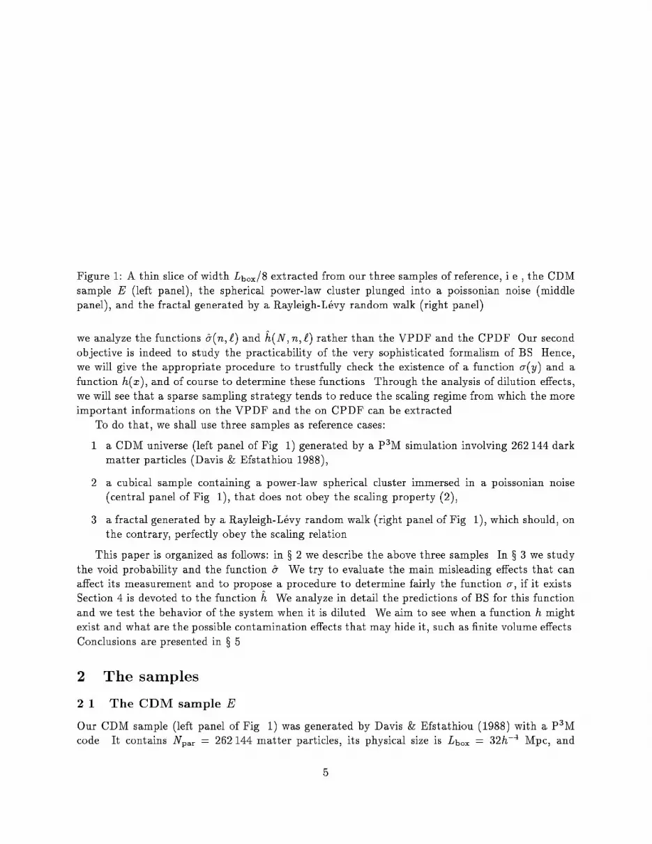
Figure 1: A thin slice of width L
box
=8 extracted from our three samples of reference, i.e., the CDM
sample E (left panel), the spherical power-law cluster plunged into a poissonian noise (middle
panel), and the fractal generated by a Rayleigh-L�evy random walk (right panel).
we analyze the functions �̂(n; `) and
^
h(N; n; `) rather than the VPDF and the CPDF. Our second
objective is indeed to study the practicability of the very sophisticated formalism of BS. Hence,
we will give the appropriate procedure to trustfully check the existence of a function �(y) and a
function h(x), and of course to determine these functions. Through the analysis of dilution e�ects,
we will see that a sparse sampling strategy tends to reduce the scaling regime from which the more
important informations on the VPDF and the on CPDF can be extracted.
To do that, we shall use three samples as reference cases:
1. a CDM universe (left panel of Fig. 1) generated by a P
3
M simulation involving 262 144 dark
matter particles (Davis & Efstathiou 1988),
2. a cubical sample containing a power-law spherical cluster immersed in a poissonian noise
(central panel of Fig. 1), that does not obey the scaling property (2),
3. a fractal generated by a Rayleigh-L�evy random walk (right panel of Fig. 1), which should, on
the contrary, perfectly obey the scaling relation.
This paper is organized as follows: in x 2 we describe the above three samples. In x 3 we study
the void probability and the function �̂. We try to evaluate the main misleading e�ects that can
a�ect its measurement and to propose a procedure to determine fairly the function �, if it exists.
Section 4 is devoted to the function
^
h. We analyze in detail the predictions of BS for this function
and we test the behavior of the system when it is diluted. We aim to see when a function h might
exist and what are the possible contamination e�ects that may hide it, such as �nite volume e�ects.
Conclusions are presented in x 5.
2 The samples
2.1 The CDM sample E
Our CDM sample (left panel of Fig. 1) was generated by Davis & Efstathiou (1988) with a P
3
M
code. It contains N
par
= 262 144 matter particles, its physical size is L
box
= 32h
�1
Mpc, and
5

it was evolved until the variance computed in a sphere of radius 8 h
�1
Mpc reached 1=b with
b = 2:5. The CPDF and the VPDF were computed by BSD for cubic cells of size ` in the
range �2:6 � log
10
(`=L
box
) � �1:0. These lower and upper limits were chosen in order to avoid
respectively smoothing and \periodisation" e�ects. In the following we shall express all lengths in
units of L
box
.
BSD have measured the functions �̂ and
^
h in the non-linear regime (�
2
> 1). In particular,
they found that
^
h did indeed scale as a function h. They proposed a phenomenological �t for
the function h, that we shall recall in x 4. They found that the transform (11) applied to this �t
reproduced well the measured function �̂. However, all this work was done at constant number
density n = 262 144. A full test of the scaling model needs n to vary. Moreover, the current
three-dimensional galaxy catalogs involve at most a few thousand objects. So to really test and
understand the scaling model and its domains of use, it will be interesting to dilute our CDM
sample that is known to exhibit the scaling properties predicted by BS.
2.2 The sample dominated by a cluster E
c
If the statistics is dominated by a single spherical and locally poissonian cluster with a power-law
average pro�le, the low-order correlations do not obey the scaling relation (2). Indeed, following
LSS, let us consider a cluster of radius R for which the number density is
n(r) = Ar
��
; r � R;
n(r) = 0; r > R; 1:5 < � < 3:
(12)
According to LSS, when r � R, the correlation function � veri�es �
2
/ r
3�2�
and the low-order
correlations scale as (Peebles & Groth 1975)
�
3
�
2
2
/ r
��3
;
�
4
�
3
2
/ r
2(��3)
: (13)
So the scaling relation is not obeyed (because � 6= 3). We have synthesized such a cluster, but for
reasons of normalization and in order to get a more realistic P
N
(`), we have immersed it into a
white noise: the density pro�le is then given by
n(r) = Ar
��
; r � R;
n(r) = AR
��
; r > R:
(14)
The cluster is located at the center of the sample, which is cubical, of size L
box
� 1. The normal-
ization < n(r) >= n implies
AR
��
�
1 +
4�
3
�
3� �
R
3
�
= n: (15)
The calculation of the two-body correlation function gives, when r � R,
�
2
(r) � 2�IA
2
n
�2
r
3�2�
; (16)
with
I =
Z
1
0
x
2��
dx
Z
1
�1
d�(x
2
+ 1 + 2x�)
��=2
: (17)
6

Figure 2: Quantities S
Q
� �
Q
=�
Q�1
2
versus scale in logarithmic coordinates as measured in E
c
for
Q = 3; 4; 5. S
Q
increases with Q. The dashed lines are power-laws of index (Q�2)(��3) (eqs. [12],
[13]).
Once � = (3 + )=2 is �xed, the choice of the number nL
3
box
of objects in the sample and of the
correlation length r
0
determines A and R. We have taken
= 1:8; r
0
= 0:087; n = 32768; (18)
which leads to � = 2:4, A = 1:7 10
�2
n and R = 0:19.
The corresponding set E
c
is displayed in Fig. 1 (central panel). Since the white noise part of
E
c
is not correlated, expressions (13) are still valid. This is illustrated by Fig. 2, which displays
quantities S
Q
, Q = 3; 4; 5 as functions of scale. The function P
N
(`), as measured on E
c
for cubic
cells of size ` in the non-linear regime (�
2
� 1) for �2:6 � log
10
(`) � �0:8, is given by Fig. 3.
At �xed scale, it presents a bump at the vicinity of its maximum, corresponding to the poissonian
noise that globally dominates the statistics (dashed curves), followed at larger N by a power-law
and a second bump above which P
N
(`) vanishes. The large N part of the CPDF is dominated
by the cluster statistics and can be easily evaluated (CBS). In particular, one can show that the
power-law part of P
N
(`) veri�es P
N
(`) / N
�3=��1
.
2.3 The Rayleigh-Levy fractal F
To have a trustable element of comparison, we have synthesized a sample F which obeys the scaling
property (2). It is a fractal involving 32 768 points generated by a Rayleigh-L�evy random-walk (see,
e.g., Mandelbrot 1975, 1982, Peebles 1980, Colombi et al. 1992). Starting from a random point in
the sample, the next point is chosen at random direction and at a distance r with a probability
p(r > `) = (`
p
=`)
�
; ` � `
p
;
p(r > `) = 1; ` < `
p
:
(19)
The process is repeated taking the new point as reference. To obtain the same two-body correlation
function as in E
c
, we chose � = 3 � = 1:2, `
p
= 1:24 10
�3
. We refer to LSS (pages 245, 248) or
7

Figure 3: Logarithm of the count probability P
N
(`) measured on E
c
as a function of log
10
N , for
various values of scale. The dashed lines correspond to the Poisson model.
Appendix A to have the expression of �
2
(r) in terms of �, n and `
p
. The �niteness of �
2
is insured
by the fact that our sample is contained in a cube of size L
box
and involves a �nite number of
objects (so F is not actually a real fractal). Figure 1 (right panel) shows a slice extracted from F
of width L
box
=8. In Appendix A, we show, generalizing a calculation of Peebles for the low-order
correlations (LSS, page 248), that this sample obeys the scaling relation (see also Hamilton & Gott
1988). We compute its function � and �nd the approximate expression
�(y) ' (1 + y=2)
�1
: (20)
The function h associated to equation (20) is
h(x) ' 4 exp(�2x): (21)
As for E
c
, we have measured the count probability for cubic cells of size ` in the scale range
�2:6 � log
10
(`) � �0:8. This sample is especially interesting, since we can exactly test on it the
predictions of the scaling model. We are able to see if they are practically veri�ed, despite the
possible misleading e�ects we describe in the following. With this sample and E
c
, we have two
extreme reference cases to decide if a function � or a function h exists or not.
3 The void probability (VPDF)
Strictly speaking, the notion of VPDF is meaningless for a continuous matter density �eld. Never-
theless, we can consider each matter particle of our CDM sample as a galaxy, as we shall do in the
following. Then, one can measure the quantity �̂(n; `) de�ned in introduction as a function of N
c
for various number densities n to have an idea of the behavior of P
0
(n; `). For example, the �rst
step is to see if the sample deviates from a pure poissonian distribution, for which �̂ � 1. Moreover,
in this system of coordinates, if the scaling relation (2) applies, �̂ should scale as a single function
�(N
c
). One may however argue that a large class of samples may exhibit a function �(N
c
), even
8

if they do not obey the scaling property. The two samples E
c
and F we have generated are here
to speci�cally address this problem. Some arti�cial deviations from the scaling relation may be
induced by misleading e�ects, such as \grid e�ects" (taking place only in numerical simulations)
and �nite sample e�ects, that are studied in detail in Appendix B. We give the main results in
x 3.4. The scaling relation may also work only in a �nite range of scales, which does not exclude
the existence of a function �(N
c
) if only this regime is taken into account.
This section is thus organized as follows: in x 3.1, we recall some aspects of the formalism of
BS. Section 3.2 studies and compares two ways of randomly diluting a sample, an analytical one
and an experimental one. In x 3.3, we measure function �̂ in E
c
and F . Section 3.4 deals with
spurious e�ects. In x 3.5, we study the scaling behavior of the function �̂ measured in our CDM
sample E.
3.1 Scaling model and VPDF
Here we assume that the scaling property (2) applies. It is argued in BS that the function �(N
c
)
should have a power-law behavior at large N
c
, i.e.,
�(N
c
) /
N
c
�1
aN
�!
c
(22)
with 0 � ! � 1 and a > 0. The measurement of � in the observed galaxy distribution is in
agreement with equation (22). The CfA data provide ! � 0:5� 0:1 (Alimi et al. 1990) and the
Southern Sky Redshift Survey (SSRS) data lead to ! � 0:7� 0:1 (Maurogordato et al. 1992). In
universes of matter coming from numerical simulations, the value of ! seems to depend on initial
conditions (see, e.g., BH). In our CDM sample, BSD have measured (for the distribution of matter
particles, whereas the previous values concern the observed galaxy distribution, which is expected
to be biased with respect to the matter distribution)
! � 0:4� 0:05: (23)
Let us de�ne the number N
v
by
P
0
� exp(�N
1�!
v
); ! < 1; (24)
and N
v
� 0 for ! = 1. The number N
v
can be considered as the typical number of objects in a cell
located in an underdense region. The typical size `
v
of a void naturally appears from the condition
N
v
(`
v
) = 1: (25)
3.2 Dilution and VPDF
The function �̂ � � ln(P
0
)=(n`
3
) in principle depends on two variables, i.e., the average number
density n and the scale `. To check if the scaling relation is ful�lled, that is if �̂(n; `) = �(N
c
), it is
useful to display �̂ as a function ofN
c
for various number densities n, to cover all the dynamic range
of possible values of (n; `). Samples of various densities can be obtained by randomly extracting
from the studied sample E some subsamples E
ran
i
(i is the number of objects) with average number
densities n
i
= n:i=N
par
. These subsamples should have the same shape and the same volume
than E, since each of them is formally a discrete realization of the same underlying density �eld
than E, but with a number density smaller than in the set E. However, in observational data
9
samples, this experimental dilution is often made by extracting several volume limited samples, so
this condition is not veri�ed, and some artifacts due to the variation of the subsamples physical
size can contaminate the measurement.
On the other hand, if the function P
N
(n; `) of E is known, this random dilution can also be
done analytically (see Hamilton 1985, Hamilton et al. 1985). Indeed, one can easily show, using
equation (4), that the CPDF P
N
(n; `), N � 1 can be obtained from the VPDF P
0
(n; `) through
the following derivation (White 1979, BS)
P
N
(n; `) =
(�n)
N
N !
@
N
@n
N
P
0
(n; `): (26)
This relation implies, by a simple Taylor expansion
P
0
(n
i
; `) =
1
X
N=0
�
1�
n
i
n
�
N
P
N
(n; `): (27)
One can moreover compute the count probability P
N
(n
i
; `) of the subsample from P
N
(n; `) by
applying equation (26) to equation (27):
P
N
(n
i
; `) =
1
X
K=N
C
K
N
�
n
i
n
�
N
�
1�
n
i
n
�
K�N
P
K
(n; `); (28)
with C
K
N
� K!=[N !(K�N)!]. The series expansion (27) converges at least for n
i
=n � 2; the VPDF
of a \subsample" denser than E can therefore be predicted, with increasing error for increasing
density. This error arises especially from the �niteness of the sample, which prevents function P
N
from being accurately calculated at large N .
Figure 4 shows �̂ as a function of N
c
, as measured in our CDM simulation (triangles) and
two randomly extracted subsamples E
ran
32768
(squares) and E
ran
1024
(pentagons). The dashed curves
represent analytical dilutions on E and on E
ran
32768
with respective dilution factors n=n
32768
= 8 and
n
32768
=n
1024
= 32. They quite superpose to the squares and the pentagons, as expected. This
measurement shows that, even if the number of points in the considered catalog is small, the direct
determination of the VPDF in this set is accurate (in the available dynamic range). In other
words, errors related to statistical poorness are small. Indeed, the analytical dilution (27) uses the
statistics of the full set E and should thus be more accurate than the experimental dilution.
One can similarly test equation (27) with n
i
=n = 2. Figure 5 displays �̂ as a function of
scale for E
ran
1024
(pentagons) and E
ran
512
(hexagons). (We use this system of coordinates to easily
distinguish between the two subsamples). The dashed curve represents the function �̂ as it should
be measured on E
ran
1024
, applying equation (27) toE
ran
512
with n
i
=n = 2. Again, the agreement between
the measurement and the prediction is good, although the two subsamples are statistically poor.
Note that the available dynamic range where the function �̂ signi�cantly di�ers from unity
of course decreases with decreasing number density n. Now, the interesting properties of a scale
invariant distribution are reached at large N
c
(eq. [22]) which of course argues against a sparse
sampling strategy. We shall discuss again this problem in x 3.5.
3.3 How signi�cant is a measurement of the function �̂?
Let us now see if at a �rst glance, the measurement of �̂ gives appropriate results for our reference
sets E
c
and F . Figure 6 shows �̂ as a function of N
c
, as measured on E
c
(left panel) and on F (right
10

Figure 4: �̂ � � lnP
0
=(n`
3
) as a function of N
c
� n`
3
�
2
in logarithmic coordinates. The triangles
refer to our CDM sample E, the squares and the pentagons to the randomly extracted subsamples
E
ran
32768
and E
ran
1024
respectively. The dashed curves correspond to an analytical dilution on E and
E
ran
32768
by a factor 8 and a factor 32 respectively; they should superpose to the squares and the
pentagons.
Figure 5: log
10
�̂ as a function of logarithm of scale in the very dilute regime. Pentagons correspond
to E
ran
1024
and hexagons to E
ran
512
. The dashed curve represents a virtual increase in number density
by a factor 2 applied to E
ran
512
. It should superpose to the pentagons.
11

Figure 6: Logarithm of �̂ as a function of logarithm of N
c
for E
c
(left panel) and F (right panel).
The �lled points correspond to the direct measurement, the stars on left panel to various analytical
dilutions varying from a factor 8 to 1024, and the open symbols to a virtual multiplication of
average number density by a factor 2. The circled points on left panel correspond to scales where
P
0
(`) � `
3
. The dotted-dashed curve on right panel is the theoretical expectation.
panel), for several number densities n
i
= 2n; n; n=8; n=39:5; n=512; n=1024 (that we also test on our
CDM sample E), using the analytical procedure given by equation (27). The stars (on left panel)
correspond to the cases n
i
< n, the �lled points to the direct measurement, and the open symbols
correspond to the case n
i
= 2n. As expected, the fractal exhibits an unique function �(N
c
), that
is quite identical to the theoretical expectation (20). The set E
c
does not scale as a function �(N
c
)
as well as F . Its function �̂ presents a plateau where �̂ � 1 and a sudden cuto� at N
c
>
�
10. The
plateau is not surprising, since E
c
is dominated by the poissonian distribution that surrounds the
central cluster. The main di�erence with a pure poissonian sample is the existence of a large range
of values of N
c
, which is provided by the presence of the cluster. A poissonian sample, that is not
correlated, has N
c
= 0. The points that verify P
0
(`) � `
3
are circled in left panel of Fig. 6. They
precisely correspond to the sharp cuto� at large N
c
. As we shall see in next section, this cuto� does
not re ect the intrinsic properties of the underlying distribution, but some special properties of the
largest void contained in this particular realization. The set F has much larger empty regions, so
none of the studied scales are susceptible to exhibit such an abnormal behavior. Therefore, with
regard to E
c
and F , a careful measurement of function �̂ seems to really re ect the underlying
behavior of the studied distribution.
3.4 Misleading e�ects
We now consider possible misleading e�ects on the VPDF. At �rst we discuss \grid e�ects" that
may take place in numerical simulations. Then, we look at �nite sample e�ects on the VPDF
and on function �̂. This section ends with a discussion on a recent measurement of function �̂ by
Vogeley et al. (1991) on the CfA catalog. We also see what happens to our CDM sample E.
12

3.4.1 Grid e�ects
Grid e�ects only exist in numerical simulations. They are linked to the fact that the information
associated to the grid of initial particle positions in the simulation has not been completely destroyed
in large underdense regions, where there is no shell-crossing. Their consequence, as shown in
Appendix B.1, is that the VPDF is arti�cially underestimated at large scales. They are negligible
when
P
0
>
�
1=e; (29)
or equivalently when N
v
<
�
1 in the formalism of BS. The scales for which P
0
< 1=e cannot be
trustfully tested and have to be removed. This decreases the available dynamic range in which the
scaling of the function �̂ scales as a function � can be tested. These e�ects do not exist in the
galaxy catalogs.
3.4.2 Finite sample e�ects and the VPDF
Practically, the measurement of VPDF is done by randomly throwing a certain number C
tot
of cells
of volume `
3
in the sample. It is then easy to show that the standard deviation on P
0
is related to
C
tot
(see for instance Hamilton 1985) through the following expression
�
�P
0
P
0
�
2
=
1
C
tot
1� P
0
P
0
: (30)
But, as already discussed for example by Maurogordato & Lachi�eze-Rey (1986), since the sample
is of �nite volume, the number of statistically independent cells C
tot
is not arbitrarily large and
may depend on average number density n and on scale `.
For a pure poissonian distribution (not correlated), a natural guess is simply
C
tot
= V
sample
=`
3
; (31)
which roughly gives the number of \statistically independent" cells of volume v = `
3
contained in
the sample. This estimation is valid for a moderately small VPDF (see Appendix B.2.1). In the
case the VPDF is very small, a correction to equation (31) is needed and C
tot
is rather of the order
of 0:07V
sample
`
�3
(n`
3
)
3
for spherical cells (see Appendix B.2.1, B.2.2).
The case of a correlated set is more complicated. Indeed, some correlations at scales larger than
the sample size are then likely to a�ect the measurement of the VPDF. It is not easy to see where
they intervene in equation (30). Our aim here is to try to clarify this situation. However, we take
a slightly di�erent approach from the one used by previous authors, which was generally based on
equation (30) (with a somewhat uncertain C
tot
).
The technical issues are detailed in Appendix B.2, where we evaluate the error associated to
�nite volume e�ects on the VPDF, assuming that the hierarchical model applies, i.e., that the
Q-body correlation function can be written as sum of products of Q� 1 terms in �
2
. We think that
the result can be reasonably generalized for any sample which does not disagree \too much" with
the hierarchical model (an independent estimation using the top hat model leads to similar results,
see Appendix B.2). The error on the VPDF is roughly approximated by
�
�P
0
P
0
�
2
' �
1
+�
2
; �
1
=
`
3
V
sample
1� P
0
P
0
; �
2
= �2(n`
3
)
2
�̂
0
�
2
(L
sample
); (32)
13

where �̂
0
� 0 stands for the partial derivative of function �̂(N
c
; n) with respect toN
c
and �
2
(L
sample
)
symbolizes the double integral of �
2
(r
1
; r
2
)=V
2
sample
over the sample volume V
sample
� L
3
sample
.
The �rst right hand side term �
1
of equation (32) can easily be understood. It is equal to the
right hand side of equation (30), with C
tot
given by equation (31). It therefore simply corresponds
to the expected \poissonian" error due to the fact that the number of statistically independent
cells of volume v = `
3
contained in the sample is �nite. As it is the case for a pure poissonian
sample, a correction to �
1
is needed when the VPDF is very small (see appendix B.2.1, B.2.2). For
practical purposes, we neglect this correction. Indeed, when it has to be taken into account, the
relative error j�P
0
=P
0
j is likely to be close to unity or larger. An other factor � depending on the
way the system is clustered [i.e., on and on the shape of function �(y)] has also been neglected
in the writing of �
1
, since it is numerically seen to be of order unity within less than a magnitude
(and it is of course exactly equal to unity in the poissonian case). The second right hand side term
�
2
of equation (32) is brought by uctuations of the underlying density �eld at wavelengths larger
than the sample size, which lead supplementary correlations.
We see that, whatever the value of the second right hand side term, there is a scale `
cut
(n)
above which the measurement of the VPDF is not statistically signi�cant. At this scale, which is
de�ned by
P
0
(n; `
cut
)
V
sample
`
3
cut
� 1; (33)
there is typically only one independent empty cell. If `
>
�
`
cut
, the VPDF is dominated by the
largest void of the sample. In a set of in�nite volume and with an in�nite number of objects (but
a �nite number density n), we should have an in�nite distribution of voids of arbitrary size. This
is not the case for a realization of �nite volume, in which the size of the largest void is necessarily
smaller than the size of the sample.
If the formalism of BS applies, �
2
can be rewritten, for N
c
� 1,
�
2
= 2!n`
3
�(N
c
)
�
2
(L
sample
)
�
2
= �2! ln(P
0
)
�
2
(L
sample
)
�
2
: (34)
One can thus expect this term to be in general small for moderately small VPDF. The poissonian
error �
1
also becomes rapidly very small if ` gets small as compared with `
cut
.
3.4.3 Finite sample e�ects and function �̂
We now wish to estimate the �nite sample error on the quantity �̂ � � ln(P
0
)=(n`
3
). Assuming that
the uncertainties �P
0
=P
0
and �n=n are small and that the indicators
e
P
0
and
e
n are statistically
independent, we might use the standard errors propagation formula and write
�
��̂
�̂
�
2
'
1
(n`
3
�̂)
2
�
�P
0
P
0
�
2
+
�
�n
n
�
2
; (35)
where
�
�n
n
�
2
=
1
nV
sample
+ �
2
(L
sample
): (36)
However, the VPDF and the number density n are strongly correlated. If n increases, then P
0
decreases. In other words, equation (35) is likely to overestimate the real uncertainty on �̂. It is
14

therefore certainly more realistic to use the following estimate
��̂
�̂
'
�
�
�
�
1
n`
3
�̂
�P
0
P
0
�
�n
n
�
�
�
�
: (37)
This writing implies that, as expected, ��̂=�̂ ' 0 when P
0
is close to unity (or, equivalently, when
n`
3
�̂ � 0), which was not the case with the more approximate evaluation (35).
When ` < `
cut
, it is easy to see that
��̂
�̂
<
�
�n
n
: (38)
This error should therefore be small if the size of the studied sample is large in comparison with
its correlation length and if nV
sample
� 1, which is the case in current observational data volume
limited subsamples, that involve at least a few hundred objects.
In fact, when one displays �̂ as a function of N
c
, a supplementary (and quite larger) error is
brought by the uncertainty on the determination of N
c
= n`
3
�
2
(see Hamilton 1993 for a detailed
study of the errors on the two-body correlation function). Indeed, the function �
2
is very sensitive to
�nite volume e�ects and is likely to be quite underestimated at large scales (CBS). The consequence
is that the measured N
c
reaches its maximum much sooner than expected. In Appendix B.3, we
estimate the error linked to the �niteness of the sampled volume on function �
2
. For a set obeying
to the scaling property, one obtains
��
2
�
2
!
2
'
S
4
4
�
2
(L
sample
): (39)
This expression is valid when the considered scale ` is small enough compared to the sample size
L
sample
(see Appendix B.3). (Note that the relative error on N
c
is slightly larger, since one has
to take also into account the error on the average number density n, which is small in comparison
with the uncertainty associated to the two-body correlation). In addition, we must not forget the
error on �
2
associated to the sample discreteness (i.e., that the number of sampled pairs is �nite,
see, e.g., Peebles 1973, LSS, p. 189 and Hamilton 1993), that we do not estimate here.
3.4.4 Comments
When Vogeley et al. (1991) measure the function �̂ in the CfA catalog, they conclude that there
is a deviation from the scaling relation at ` � 10h
�1
Mpc. But at such a large scale, the measured
number N
c
is, as discussed above, likely to be underestimated. Moreover, the measured function �̂
becomes an increasing function of ` because the sample is dominated by its largest void (Appendix
B.2.2). In this case, the measurement of P
0
is not statistically signi�cant, so no conclusion can be
reached about the scaling behavior of the underlying galaxy distribution at such scales, not because
the scaling does not exist, but because the sample is too small. This point has also been discussed
by Maurogordato et al. (1992).
With regard to our CDM sample E, we know from CBS that �nite volume e�ects are negligible
on N
c
in the scaling range measured. Such e�ects should be even less signi�cant on function �̂.
Actually, grid e�ects are here more important than �nite volume e�ects, and the condition P
0
� 1=e
is stronger than the condition ` < `
cut
.
15

3.5 Extracting the possibly scaling part of the VPDF
In Fig. 7, we give �̂ as a function of N
c
for E, and several subsamples extracted at random (with
32768, 6634, 1024 and 512 objects). Open triangles represent a virtual increase of the average
number density of E by a factor 2. The points for which P
0
< 1=e have been removed, although
grid e�ects should be less signi�cant for randomly diluted subsamples, particularly if the dilution
factor is large. Indeed, the information linked to a grid is partially destroyed by random dilution.
The deviation from the scaling, even if it still exists, is much less apparent than in Fig. 4. But as
noticed above, removing the scales for which P
0
� 1=e decreases the available dynamic range and
improves the apparent existence of a function �(N
c
).
We also know from the measurement of the low-order averaged matter correlations (CBS) in
this sample that there should be a deviation from the scaling relation when log
10
` > �1:6, because
of the transition around `
0
between the highly non-linear regime and the weakly non-linear regime,
that exhibit here di�erent values of S
Q
for Q � 5 (see also x 4.2.1 hereafter). To measure the
function �, if it exists, one must at �rst select the scale range L
scaling
where the scaling relation
is expected to apply. The measurement of the low-order correlations provides at least the upper
bound of L
scaling
(the lower bound of L
scaling
is di�cult to evaluate in numerical samples, because
at very small scales, the low-order correlations are a�ected by discreteness and also by numerical
errors linked to the smoothing of the forces in the program solving the equations of motion). This
measurement must be done with care, since even the low-order correlations are quite sensitive
to �nite sample e�ects (CBS). In Fig. 7, the points that verify log
10
` � �1:6 are circled. They
unambiguously de�ne a single function �(N
c
). This proves that the measured low-order statistics
is here in agreement with the measured high-order statistics (function �̂ is related to the behavior
of the averaged correlations at any order), as far as the scaling relation is concerned.
The dotted-dashed curve in Fig. 7 is the function �(N
c
) predicted by the transformation (11)
applied to the function h(x) measured on E by BSD (see x 4.1). It is in very good agreement with
the measurement (circled points). This proves that with careful measurements, the predictions of
BS are obeyed in a great detail, even on relations between indicators that describe very di�erent
regions of the studied sample: the function �(N
c
) tests underdense regions, whereas the function
h(x) tests overdense places.
Note however that the very dilute subsamples (n � 6634) provide at most N
c
� 2 when
log
10
(`) � �1:6: at such a N
c
, the asymptotic power-law behavior (22) of � is not reached,
although � already signi�cantly deviates from the Poisson expectation (� = 1). With regards
to the perfectly scale invariant fractal F , for n = 6634, we have N
c
(`
0
) � 40. With smaller values
of N
c
(especially smaller than 10), we would still miss the large-N
c
power-law behavior of �. This
suggests a lower bound on N
c
to determine the power-law behavior of �: it has at least to be larger
than a few tens at the correlation length, that is n`
3
0
>
�
30 � 40, or, in terms of galaxy number
density (`
0
' 2:4r
0
' 12h
�1
Mpc)
n
>
�
0:02� 0:03h
3
Mpc
�3
: (40)
This average number density is hardly reached by current observational volume limited subsamples
extracted from data samples, in which n is at most of order 0:01h
3
Mpc
�3
, or equivalently N
c
(`
0
) �
15. This, of course, argues against any sparse sampling strategy. Indeed, since the VPDF is not
very sensitive to �nite volume e�ects, it is more important to have a small but as complete as
possible catalog than a large dilute sample to measure the function �̂.
16

Figure 7: �̂ as a function of N
c
in logarithmic coordinates, as measured in our CDM sample E, and
several subsamples extracted at random. The open triangles represent the measurement on a virtual
sample twice denser than E, using the analytical prescription (26). The points for which P
0
< 1=e
have been removed. The circled points verify log
10
` � �1:6. In this scale range, the low-order
correlations obey the scaling relation. The dotted-dashed curve is the analytical transformation
(11) applied to the function h BSD have measured on E.
17

4 The count probability distribution function (CPDF)
In the scaling model framework, it is useful to measure the quantity
^
h(N; n; `) � N
c
�
2
P
N
(n; `) as a
function of x = N=N
c
, for various values of (n; `). Indeed, when the scaling relation (2) applies,
^
h
behaves like an universal function function h(x) in an asymptotic domain D
h
. Practically, however,
this asymptotic regime is never completely reached and one can expect some contamination e�ects
to modify the behavior of function
^
h(N; n; `) so that it does not scale exactly as a function h(x).
For example, the high N part of the function P
N
(n; `) presents increasingly large irregularities as
N grows and a brutal cuto� at �nite N , because of the sample volume �niteness, as shown by CBS.
Now, the CPDF is usually studied through its reduced moments, e.g., the averaged correlation
functions �
Q
. Unfortunately, the measurement of such functions is very sensitive to the �niteness
of the sampled volume. CBS have studied in detail such �nite volume e�ects on the CPDF, and
concluded they could lead to a systematic, strong, underestimation of the real low-order moments
of the CPDF with direct measurements. They proposed a method to correct for such defects, or
at least to estimate fair errorbars. We shall recall below their main results.
Once all spurious e�ects are known, one can wonder if the apparent existence of a function h
is not more or less systematic whatever the studied sample. In such a case, the formalism of BS
would be useless. Once we will be convinced that this is not the case, we shall be able to see to
what extent it is possible to detect a function h(x) in the observed galaxy distribution.
This section is thus organized as follows: in x 4.1, we give D
h
and the main properties of function
h, that have been computed by BS. We study contamination e�ects brought by discreteness and
�nite sample e�ects in x 4.2 (where we recall the main results of CBS). In x 4.3, we measure function
^
h on the three reference samples E, E
c
and F . By randomly diluting our CDM sample E, we also
see what occurs when the number density of the sample becomes comparable to which is reached
in current three-dimensional observational data samples. We then try to determine a criterion on
the galaxy number density to measure the interesting scaling behavior of function
^
h, as we did for
the VPDF.
4.1 Some aspects of the scaling model linked to overdense regions
Here we recall some predictions of BS based on the scaling relation (2).
The invariance property (9) is expected to be reached in the scale and number domain D
h
given
by
D
h
� f`
c
� `� `
0
; N � 1; N � N
v
g : (41)
`
0
� 2:4r
0
is the (pseudo-)correlation length for which the averaged two-body correlation is unity:
�
2
(`
0
) � 1: (42)
The scale `
c
is de�ned by
N
c
(`
c
) � 1: (43)
It is the typical distance between two objects in a cluster. When ` � `
c
, the system becomes
quasi-poissonian, i.e., �(N
c
) � 1. The condition N � 1 is linked to discreteness e�ects. If N
v
� 1,
the CPDF presents at low N (N � N
v
) an exponential cuto� which scales as a function g. The
latter is completely determined once ! is known (eq. [22]), so its main interest is to help for the
measurement of !, in the case the scaling relation applies.
18

The function h should behave at small x as a power-law:
h(x) � x
!�2
; x� 1; (44)
and it presents at large x an exponential cuto�
h(x) � exp(�jy
s
jx); x� 1: (45)
It must also obey the normalization conditions (see, e.g., BS)
Z
1
0
xh(x)dx � 1;
Z
1
0
x
2
h(x)dx � 1: (46)
The CPDF measured in our CDM sample was found by BSD to scale properly and determine a
unique function h when (N; `) � D
h
(see also x 4.3 hereafter). BSD have �tted h with the following
phenomenological form
h
�t
(x) = a
(1� !)
�(!)
x
!�2
e
�jy
s
jx
(1 + bx)
c
; (47)
which, of course, obeys the normalizations (46), follows the small-x power-law behavior (44) and
has an exponential cuto� (45) at large x with jy
s
j � 0:125. The parameters a � 1:8 and ! � 0:4 are
determined by the measurement of �(N
c
) at large N
c
(see eq. [22], and also by the measurement of
function g, see, e.g., BSD). The parameter jy
s
j is determined by the measurement of function h at
large x. The remaining parameters b � 3:6 and c � 0:8 are determined by the two constraints (46).
4.2 Misleading e�ects on the CPDF and on function
^
h
4.2.1 CPDF and �nite volume e�ects
The CPDF, as it is measured in universes of matter coming from N -body simulations (see, e.g.,
BSD, BH, CBS) or in the galaxy distribution (see, e.g., Alimi et al. 1990), is seen to present, in the
non linear regime, an exponential tail at large N , with irregularities more and more pronounced as
N increases and a brutal cuto� at a �nite N = N
max
, above which P
N
= 0. This is illustrated by
�gure 8, which displays the quantity log
10
N
2
P
N
measured in our CDM sample E as a function of
N . In current observed three-dimensional galaxy catalogs, for example the SSRS catalog analysed
by Maurogordato et al. (1992), these irregularities are so pronounced that the exponential tail of
the CPDF is di�cult to detect. CBS have shown that such irregularities are due to the fact that, at
large N , the CPDF is dominated by a few large clusters in the sample, each bump corresponding to
a cluster. The last bump presented by each curve (for �2:0
<
�
log
10
`
<
�
�1:6) on Fig. 8 corresponds
to the largest cluster in our CDM sample (see CBS for a detailed modelization and discussion).
Such irregularities and the brutal cuto� at N
max
are of course spurious. In a larger sample, the
cuto� and the bumps would appear further down the large-N tail of the CPDF: the bumps in the
smaller sample would now be smoothed by statistical averaging. Indeed, in an in�nite volume, one
can �nd an in�nite number of clusters of any sizes. The exponential tail shown up by the CPDF
at large N should thus be extended to in�nity. Of course, the range of the exponential tail that
brings a substantial contribution to any statistics depends on that statistics, and it does not need
to be known with precision at arbitrarily large N . It can be modeled in the following way
P
N
(`) � A(`)N
�(`)
e
��(`)N
; (48)
19

Figure 8: Logarithm of the quantity N
2
P
N
(`), measured in our CDM sample, as a function of N .
Each curve corresponds to a given choice of scale. The scale decreases from the top curve (for
which we have log
10
` = �1:0) to the bottom curve (for which we have log
10
` = �2:6) with a
logarithmic step � log
10
` = 0:2. The smooth lines are the analytical �t given by eq. (48). This
�gure is extracted from CBS.
with
�(`) = jy
s
(`)j=N
c
(`): (49)
The functions �(`) and jy
s
(`)j are expected to slowly vary with scale (and to be constant if the
scaling relation applies, see x 4.1), and the quantity A(`) is a normalization factor (the best �t
values of �(`) and jy
s
(`)j can be found in CBS).
Let us now turn to the Q-body averaged correlation functions �
Q
. When the order Q increases,
the weight given to high density regions is larger and larger and the defects described above, partic-
ularly the cuto� of the CPDF at N
max
, have stronger and stronger in uence on the measurement of
�
Q
. Such measurement would be more realistic if one extended to in�nity the exponential tail (48).
To illustrate this point, �gure 9 displays in logarithmic coordinates the quantities S
Q
� �
Q
=�
Q�1
2
,
3 � Q � 5, as functions of �
2
, measured in E and in a larger CDM realization E
L
(with a box
size L
box
= 90h
�1
Mpc). The underlying statistics in E and E
L
is theoretically exactly the same,
but the set E
L
is of much larger size than E compared to the correlation length and is thus ex-
pected to be much less contaminated by �nite volume e�ects. The solid curves with triangles and
squares correspond respectively to direct measurements of functions S
Q
in the sets E and E
L
. They
undoubtly disagree between each other. But once �nite volume e�ect in E have been corrected
by extending the exponential tail at large N of the CPDF to in�nity, one obtains a much better
agreement (dashed curves). The same procedure applied to E
L
does not signi�cantly change the
results. The above discussion shows that the method proposed by CBS to correct for �nite volume
e�ects is e�cient (more tests are made in CBS to test the viability and the uncertainties of the
method). Note that, in the sample E, the plateau exhibited by S
Q
in the highly non linear regime
(�
2
� 1) is hidden by �nite volume e�ects, before correction.
20

Figure 9: Logarithm of the quantity S
Q
� �
Q
=�
Q�1
2
, 3 � Q � 5, measured in our CDM sample E as
a function of �
2
. The order Q increases with S
Q
. The �lled triangles refer to E, the open triangles
correspond to the same quantity, but corrected for �nite volume e�ects and the squares refer to
the larger CDM sample E
L
. Consistency between E and E
L
is only insured after correction. This
�gure is extracted from CBS.
4.2.2 Misleading e�ects on function
^
h
Practically, the regime de�ned by equation (41) is never reached, even in very large samples such
as our CDM sample, that involve more than 2:10
5
points. In three dimensional galaxy catalogues,
that contain at most a few thousand objects, `
c
is close to `
0
(at best of order `
0
=10) and the
constraint `
c
� ` � `
0
is not veri�ed. Then, the asymptotic regime (9) is hardly reached and the
formalism of BS may be useless in this case.
Hence, let us assume that we have a sample of �nite volume at our disposal, involving a �nite
number of objects and being a realization of a scale invariant underlying distribution. We evaluate
here deviations from the invariance property (9) brought by the �niteness of the sampled volume
and related to the fact that instead of equation (41), one practically has
`
c
<
�
`
<
�
`
0
; N
>
�
1; N
>
�
N
v
: (50)
To study separately the various misleading e�ects that can hide function h, we formally write
(although the two terms A
dis
and A
�n
explained hereafter can be correlated each other)
^
h(N; n; `) = U(N; `; n):h(x); (51)
with
U(N; `; n) = [1 +A
dis
(N; n; `)]:[1+ A
�n
(N; `)]: (52)
The �rst factor of equation (52), 1 + A
dis
, accounts for discreteness e�ects and for the deviation
from the scaling behavior of the system in underdense regions (N � N
v
). It has been evaluated
by BSD, assuming that function �(N
c
) has reached its expected power-law behavior (22) at large
N
c
(with the notations of BSD, we have 1 + A
dis
= 1=a
N
). Note that the quantity A
dis
computed
21

by BSD depends on the parameter ! de�ned in equation (22). In appendix C.1, we study A
dis
in
terms of moments of the CPDF (without making any assumption on function �). For example, in
the vicinity of N � N
c
, the quantity 1 +A
dis
should be roughly of the same order as
1 + A
dis
(N; n; `) � 1 + 1=N
c
+ 1=�
2
; N � N
c
: (53)
This estimate is only very approximate, because it does not take into account the complex behavior
of the number A
dis
as a function of N . Of course, in the limit N � 1, N � N
v
and `
c
� `� `
0
,
A
dis
vanishes.
The second factor, 1 + A
�n
, is related to �nite volume e�ects, that are widely discussed in
previous section. Because of the �niteness of the sampled volume, the CPDF presents irregularities
at large N followed by a sharp cuto� at N = N
max
(n; `), instead of the smooth exponential tail
predicted at large x for function h (eq. [45]). These e�ects have been carefully studied by CBS. A
cuto� at large N on the CPDF changes the overall normalizations. Indeed, 1+A
�n
is given, in the
vicinity of N
c
, by
1 +A
�n
(N; `) � 1
,
Z
N
max
=N
c
0
x
2
h(x)dx > 1: (54)
This result is valid only if the two-body correlation is not a�ected by �nite volume e�ects when
`
<
�
`
0
, which should be the case of any reasonable sample. When the sample size gets larger, the
ratio N
max
=N
c
increases. In the limit of an in�nitely large sample, 1+A
�n
goes of course to unity.
4.3 Is there a function h or not?
We can see, from results of previous section, that the measurement of function
^
h, in the framework
of the scaling model, is quite delicate. When the above defects are important, it may be very
di�cult to distinguish between a sample which obeys the scaling property and a sample which does
not. Here, we measure function
^
h on the two reference samples E
c
, F , and on the more realistic
set E and its various subsamples obtained by random dilution. Our aim is to prove that a careful
measurement of function
^
h allows one to successfully test the predictions of BS, if the considered
sample is rich enough, which is not yet the case for current three-dimensional observational galaxy
catalogs.
Following BSD and BH, our practical implementation
e
D
h
of the asymptotic domain D
h
(see
eq. [41]) is
e
D
h
=
n
N
c
> 1:8; `=`
0
< 0:4; N � 1; N > 4N
v
; NP
N
`
�3
> 8
o
: (55)
The supplementary last condition comes down to removing the very large N part of the CPDF,
where this latter is dominated by �nite volume e�ects (c.f. BSD and BH). To enlarge the available
dynamic range, we will divide when possible the measured function
^
h by the factor 1+A
dis
computed
by BSD, to correct for discreteness e�ects. This explains why we take N � 1 instead of N � 1. Of
course, we can still expect signi�cant di�erences between function
^
h and the the searched function
h, due to the factor 1 +A
�n
(N; `).
This section is organized as follows: in x 4.3.1, we measure function
^
h in the sets E
c
and F . We
want to check if these two reference samples give the expected results, knowing that F is obeying
the scaling relation and that E
c
does not verify it. In x 4.3.2, we measure function
^
h in the CDM
sample E, and its various subsamples randomly extracted. The idea is to dilute E to reach the
same number density n as in current observational galaxy samples. This section is concluded by
22

Figure 10: Function x
2
^
h(N; `) � N
2
P
N
(`)=(n`
3
) as a function of x � N=N
c
as measured in the
fractal F in logarithmic coordinates. Only the values (N; `)�
e
D
h
(where
e
D
h
is de�ned by equation
[55]) have been selected. The dashed curve is the theoretical expectation h(x) = 4 exp(�2x).
x 4.3.3, where we give constraints on n to detect a function h (when it exists) and to fairly measure
it.
4.3.1 The reference samples
The samples E
c
and F involve a large number of points N
tot
= 32 768. In these sets, we have
`
c
=`
0
' 0:016, so the e�ective dynamic range
e
D
h
should be large.
Figure 10 displays the quantity x
2
^
h(N; `) (n = 32; 768)measured on F as a function of x = N=N
c
for (N; `)�D
h
(we take here ! = 1, as suggested by the theoretical calculation of Appendix A and
the measurement of function � in x 3.3, so N
v
� 0). Note that if we took all the available values
of (N; `), the result would be very similar, which explains why we do not show the corresponding
panel. The function h is unambiguously detected: all the curves have the same shape and superpose
very well. The dashed line is the theoretical expectation, which is in a good agreement with the
measurement.
Left panel of Fig. 11 shows the quantity x
2
^
h(N; `) (n = 32 768) measured in E
c
as a function of
x = N=N
c
. As expected, the curves are not signi�cantly more gathered than in Fig. 3, which is a
�rst indication against the existence of a function h. Right panel of Fig. 11 is the same as left panel,
but only the values of (N; `) that belong to
e
D
h
have been taken into account. Here, we have not
corrected for discreteness, since the value of ! = 0 we get from function �̂ (x 3.3) would call for a
special treatment that we felt not necessary to write out. We have however taken N � 2 instead of
N � 1 to remove the regime completely dominated by discreteness. The scattering of the curves is
much smaller in right panel of Fig. 11 than in left panel, which is not surprising since the available
dynamic range has been reduced. This could give the misleading illusion that a function h exist, but
this scattering is about an order of magnitude, much larger than the expected maximal scattering
S that can be infered from equation (53). We indeed �nd log
10
S = max[log
10
(1 + A
dis
)] � 0:2 in
the scale range given by equation (55). We do not take into account here possible �nite volume
e�ects (that are in some way an intrinsic feature of this sample that contains only one cluster). In
other words we assume 1 +A
�n
' 1. The computation of 1 +A
�n
indeed needs to guess a possible
function h (eq. [54]), which is quite di�cult for this particular case, as can been seen on Fig. 11.
23
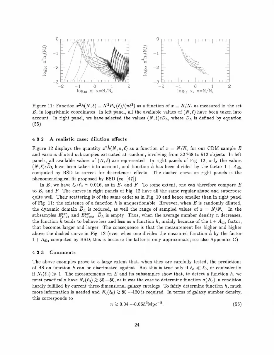
Figure 11: Function x
2
^
h(N; `) � N
2
P
N
(`)=(n`
3
) as a function of x � N=N
c
as measured in the set
E
c
in logarithmic coordinates. In left panel, all the available values of (N; `) have been taken into
account. In right panel, we have selected the values (N; `)�
e
D
h
, where
e
D
h
is de�ned by equation
(55).
4.3.2 A realistic case: dilution e�ects
Figure 12 displays the quantity x
2
^
h(N; n; `) as a function of x = N=N
c
for our CDM sample E
and various diluted subsamples extracted at random, involving from 32 768 to 512 objects. In left
panels, all available values of (N; `) are represented. In right panels of Fig. 12, only the values
(N; `)�
e
D
h
have been taken into account, and function
^
h has been divided by the factor 1 + A
dis
computed by BSD to correct for discreteness e�ects. The dashed curve on right panels is the
phenomenological �t proposed by BSD (eq. [47]).
In E, we have `
c
=`
0
' 0:016, as in E
c
and F . To some extent, one can therefore compare E
to E
c
and F . The curves in right panels of Fig. 12 have all the same regular shape and superpose
quite well. Their scattering is of the same order as in Fig. 10 and hence smaller than in right panel
of Fig. 11: the existence of a function h is unquestionable. However, when E is randomly diluted,
the dynamic domain
e
D
h
is reduced, as well the range of sampled values of x = N=N
c
. In the
subsamples E
ran
1024
and E
ran
32768
,
e
D
h
is empty. Thus, when the average number density n decreases,
the function
^
h tends to behave less and less as a function h, mainly because of the 1 +A
dis
factor,
that becomes larger and larger. The consequence is that the measurement lies higher and higher
above the dashed curve in Fig. 12 (even when one divides the measured function
^
h by the factor
1 +A
dis
computed by BSD; this is because the latter is only approximate; see also Appendix C).
4.3.3 Comments
The above examples prove to a large extent that, when they are carefully tested, the predictions
of BS on function
^
h can be discrimated against. But this is true only if `
c
� `
0
, or equivalently
if N
c
(`
0
) � 1. The measurements on E and its subsamples show that, to detect a function h, we
must practically have N
c
(`
0
)
>
�
30� 50, as it was the case to determine function �(N
c
), a condition
hardly ful�lled by current three-dimensional galaxy catalogs. To fairly determine function h, much
more information is needed and N
c
(`
0
)
>
�
80� 120 is required. In terms of galaxy number density,
this corresponds to
n
>
�
0:04� 0:06h
3
Mpc
�3
: (56)
24

Figure 12: Logarithm of x
2
^
h(N; n; `) as a function of log
10
N as measured on E (a), E
ran
32768
(b),
E
ran
6634
(c), E
ran
1024
(d) and E
ran
512
(e). All the available values of (N; `) are used in left panels. In
right panels, only the values of (N; `)�
e
D
h
have been taken into account. For E
ran
1024
and E
ran
512
,
e
D
h
is
empty. We have corrected for discreteness e�ects at small N . The dashed curve is the analytical
�t of BSD (eq. [47]). A shift increasing with decreasing number density can be observed between
the measurement and this dashed curve. It is essentially due to the fact that `
c
is approaching `
0
while the sample is diluted, which reduces the domain
e
D
h
where the behavior of function
^
h(N; n; `)
as a function h(N=N
c
) is expected.
25

Moreover, the size of the sample has to be large in comparison with the correlation length, otherwise
�nite volume e�ects will make the exponential tail presented by function h at large x undetectable.
Constraint (56) is quite stronger than equation (40), which de�nitely argues against sparse sampling
strategies. Of course, the speci�c case of our CDM sample cannot be generalized to arbitrary set
of points. The work of Maurogordato et al. (1992) on the SSRS catalogue provides rather good
indications of the scaling of the CPDF measured in this sample as a function h, although their
volume limited samples had n at most of order only a few 10
�3
h
�3
Mpc
3
. But because `
c
is close
to `
0
, they use a domain
e
D
0
h
larger than which is given by equation (55). As it would be the case
if we measured the function
^
h in E
ran
512
and E
ran
1024
[see panels (e) and (f) of Fig. 12] in
e
D
0
h
, their
function
^
h is quite noisy, since the scaling as a function h is expected to be less good in this case.
Furthermore, because of the small size of their volume limited sample, their measurement is quite
contaminated by �nite volume e�ects.
5 Summary and conclusions
We have measured the count probability in three samples, i.e., a power-law spherical cluster E
c
plunged in a poissonian distribution involving 32 768 objects, a fractal F generated by a Rayleigh-
L�evy random walk involving 32 768 objects, and a CDM sample E involving 262 144 matter parti-
cles.
We have evaluated errors due to various spurious e�ects, such as �nite volume e�ects, dis-
creteness e�ects and \grid" e�ects on the void probability (VPDF) and on the count probability
(CPDF). Our study has been made in the framework of the scaling model. We indeed wanted to
test the practicability and the viability of the formalism of BS. The main results are the following:
5.1 About the VPDF and the function �̂
1. The VPDF exhibits little sensitivity to �nite sample e�ects, except at the larger scales where
it rapidly deteriorates. The trustable scales are smaller than the scale `
cut
de�ned by
P
0
(n; `
cut
)V
sample
`
�3
= 1; (57)
where V
sample
is the sample volume. Above this scale, the measurement of the VPDF is not
statistically signi�cant. For `� `
cut
the error on function �̂ � n
�1
`
�3
ln P
0
should be roughly
smaller than the uncertainty on the average number density
�n
n
=
h
(nV
sample
)
�1
+ �
2
(L
sample
)
i
1=2
; (58)
where �
2
(L
sample
) is the average of function �(r
1
� r
2
) over the sampled volume. This error
is expected to be very small.
2. However, when one wants to test the scaling model, the quantity �̂ is studied as a function of
N
c
= n`
3
�
2
. This scaling number N
c
is rather sensitive to �nite volume e�ects. It is indeed
likely to be systematically underestimated by a direct measurement at large scales (CBS).
The �nite volume error on this number can be approximated by
�
�N
c
N
c
�
2
' [1 + S
4
=4] �
2
(L
sample
): (59)
26

This evaluation assumes that the hierarchical model applies (see Appendix B.3). It does not
give the amount of the systematic underestimation quoted above but rather estimates the
uncertainty on the overall normalization of N
c
.
3. In numerical simulations, a supplementary spurious e�ect is expected if the initial distribution
of particles was a slightly perturbed regular pattern. This way of setting initial conditions,
good from a numerical point of view, because it minimizes white noise at small scales, is bad
from a statistical point of view, since it brings some unexpected correlations, that we call grid
e�ects. The consequence is that the VPDF is underestimated, particularly at large scales.
Grid e�ects should be negligible only if
P
0
(n; `)
>
�
e
�1
; (60)
which is a rather severe restriction.
4. Once all spurious e�ects are known and have been isolated, the scaling model can be trustfully
tested on the function �̂. The procedure consists in measuring the quantity �̂(n; `) as a
function of N
c
in the sample and in various subsamples randomly extracted. This can also
be done analytically, using equation (27). Then, if the scaling relation applies in a given
scale range, that can be determined by carefully measuring the low-order correlations (CBS,
x 4.2.1), an unique function �(N
c
) can be determined.
5. To have signi�cant information on the asymptotic behavior of function �̂, larges values of N
c
are needed. We �nd with practical measurements that N
c
should at least verify
N
c
(`
0
)
>
�
30� 40; (61)
where `
0
is the correlation length, for which �
2
(`
0
) = 1. In terms of galaxy number density,
this gives n
>
�
0:02� 0:03h
3
Mpc
3
. This number is hardly reached by current volume limited
three-dimensional galaxy catalogs. This strongly argues against sparse sampling strategies.
5.2 About the CPDF and function
^
h
If the scaling relation applies, the function
^
h(N; n; `) � N
2
c
n
�1
`
�3
P
N
(n; `) should scale as an
universal function h(N=N
c
), that is characteristic of the underlying continuous density �eld and
has some speci�c properties computed by BS. However, this behavior is only asymptotic, for a
large number of sampling points, and the function
^
h(N; n; `) is never exactly equal to function
h(x), which makes the detection and the measurement of function h somewhat delicate.
1. A small N , discreteness e�ects dominate soN � 1 is required. Moreover, underdense regions,
that have a di�erent scaling behavior contaminate the measurement, so N � N
v
is required.
But such constraints are di�cult to follow in realistic samples. Fortunately, BSD found a way
to correct for discreteness and the in uence of underdense regions, so that one can enlarge
the available dynamic range to N
>
�
1 and N
>
�
N
v
. However, their correction needs some
improvements (i.e., must be generalized with weaker hypotheses, Schae�er et al. 1994).
2. Real sample are of �nite volume. The consequence is a sharp cuto� at large N on the CPDF.
It implies that low order moments of the CPDF are likely to be underestimated by direct
measurements. CBS have proposed a method to correct for such defects, which consists in
27
extending to in�nity the exponential tail presented by the CPDF at largeN . One consequence
of �nite volume e�ects is also a change in the overall normalization of function
^
h, which is
larger than expected in the vicinity of N � N
c
. Unfortunately, the corresponding factor
1 + A
�n
between functions
^
h and h is easy to evaluate only if the scaling relation is obeyed,
since one has to know the function h to compute it.
But once these defect have been carefully taken into account, it is seen that the scaling model
formalism can be used. However, to trustfully decide if a function h exists or not, condition (61) is
required. To measure this function without having to introduce strong corrections, we must require
N
c
(`
0
)
>
�
80� 120: (62)
In terms of galaxy density, we thus must roughly have n
>
�
0:04� 0:06h
�3
Mpc
3
, a constraint that
is not ful�lled by current volume limited three dimensional galaxy catalogs.
5.3 Perspectives
Our count probability cook book is far from being complete, since we have not taken into account
observational e�ects, such as selection and redshift e�ects. Moreover, we have only studied the
speci�c case of the scale invariant model of BS. Other models, such as the lognormal distribution
(Coles & Jones 1991), the negative binomial model and the thermodynamic model of Saslaw and
Hamilton (1984) also provide very good �ts of the measured count probability in the observed galaxy
distribution (Crane & Saslaw, 1986, 1988). Actually, all these models were seen by Bouchet et al.
(1991, 1993) to become indistinguishable in the scaling regime available in the galaxy distribution.
As argued by Bouchet et al., this is certainly because the current galaxy catalogs are too sparse
and widely dominated their discrete nature (so conditions [61] and [62] are of course not ful�lled),
but this issue has to be further clari�ed.
Acknowledgments. SC is supported by DOE and by NASA through grant NAGW-2381 at
Fermilab. Part of this work was done while SC was at the Institut d'Astrophysique de Paris
(CNRS), supported by Ecole Polytechnique, and at the Lick Observatory (UCSC), invited by L.
Hernquist.
APPENDIX
A distribution function of our fractal F
Here we compute the statistical properties of our fractal F . At �rst, we compute the Q-body
correlation functions, redoing in a slightly di�erent way a calculation of Peebles (LSS), and show
that this set obeys the scaling relation. Then, we try to evaluate functions �(y) and h(x).
A.1 Computation of the Q-body correlations
The mean number density n of a real fractal generated by an in�nite Rayleigh-L�evy random walk
diverges. Moreover, such a set has no correlation length, i.e., �
2
is in�nite. By imposing that F is
a replicated cubical box involving a �nite number of objects, we assure the �niteness of n and �
2
.
28

To test a more realistic situation, we follow LSS and assume here that our set F is generated by
a distribution of �nite random walks W
i
, with a random number N
i
of steps, started at a random
place of the sample, so that the average number density n
W
of chains veri�es n = n
W
: < N
i
>.
Mandelbrot (1975) and Peebles (LSS, p. 245) give the probability density f(r) of a displacement
r after any number of steps in a given walk W
i
. With the notations of x 2.3, we have
f(r) = Cr
�
; = 3� �; � < 2; (63)
with
C =
(�+ 1)(�� 1)
2�
2
tan
�
�
�
2
�
�
`
��
p
: (64)
In the following, we shall use the notation
r
l;m
= jr
l
� r
m
j: (65)
We now want to compute the two-body correlation function. Let �P be the probability of
�nding an object in both of the volume elements �V
1
and �V
2
. The probability that the two objects
have been generated by the same walk W
i
is �P
1
= [f(r
1;2
) + f(r
2;1
)]n�V
1
�V
2
. The �rst term says
that the object 2 have been generated after the object 1 with a probability f(r
1;2
)�V
2
(and the
probability of existence of object 1 is n�V
1
), but the reverse way is possible (term with r
2;1
). The
probability that the two objects have been generated by W
i
and W
j
with i 6= j is �P
2
= n
2
�V
1
�V
2
,
since W
i
and W
j
are not correlated each other. By de�nition of the two-body correlation, we have
�P � [1 + �
2
(r
1;2
)]n
2
�V
1
�V
2
= �P
1
+ �P
2
. So we get
n�
2
(r
1
; r
2
) = 2Cr
�
1;2
: (66)
Let us compute the three-body correlation function. Let �P be the probability of �nding three
objects respectively in the three volume elements �V
1
, �V
2
and �V
3
. We have then three possibilities.
The �rst one is that the three objects have been generated by the same walk W
i
; the probability of
such an event is �P
1
= [f(r
1;2
)f(r
2;3
) + cyc:+ rev:]n�V
1
�V
2
�V
3
(the term \cyc." take into account
all the possible paths that can cross the three objects (three terms), and \rev." indicates that
the reverse way is possible). The second possibility is that two objects have been generated by a
walk W
i
and the other object have been generated by W
j
with i 6= j; the probability of such an
event is �P
2
= [f(r
1;2
)+f(r
2;3
)+f(r
3;1
)+rev:]n
2
�V
1
�V
2
�V
3
. The third possibility is that the three
objects have been generated by three di�erent walks; its probability is �P
3
= n
3
�V
1
�V
2
�V
3
. By
de�nition of the three-body correlation function �
3
, we have �P � [1+�
2
(r
1;2
)+�
2
(r
2;3
)+�
2
(r
3;1
)+
�
3
(r
1;2
; r
2;3
; r
3;1
)]n
3
�V
1
�V
2
�V
3
= �P
1
+ �P
2
+ �P
3
. So we get
�
3
(r
1
; r
2
; r
3
) = [�
2
(r
1;2
)�
2
(r
2;3
) + cyc: (3 terms)]=2: (67)
Let us compute the Q-body correlation function. Let �P be the probability of �nding N objects
respectively in the Q volume elements �V
1
,...,�V
Q
. As we did for the two-body and the three-body
correlation functions, we have to �nd all the possible combinations of sets W
i
and paths in W
i
.
Let P be the set of partitions of the set f1; :::; Qg. An element of P is written i = (i
1
; :::; i
s
),
with i
k
= fi
k;1
; :::; i
k;card(i
k
)
g. With these de�nitions, we thus have i
k
\ i
l
= ; if k 6= l, and
i
1
[ :::[ i
s
= f1; :::; Qg. In the following, we use the notation card(i
k
) = c
k
. Generalizing the above
procedure, we �nd
�P = �V
1
:::�V
Q
X
(i
1
;:::;i
s
)�P
s
Y
k=1
X
permutations j[i
k
]
nf
j
1
;j
2
� :::� f
j
c
k
�1
;j
c
k
; (68)
29

with
X
permutations j[i
k
];c
k
=1
nf
j
1
;j
2
� :::� f
j
c
k
�1
;j
c
k
� n; (69)
and f
l;m
� f(r
l;m
). Now we have
�P � n
Q
�V
1
:::�V
Q
X
(i
1
;:::;i
s
)�P
s
Y
k=1
�
c
k
(r
i
k;1
; :::; r
i
k;c
k
); (70)
with �
1
� 1. It is then easy to recursively compute the Q-body correlation function:
�
Q
(r
1
; :::; r
Q
) = [�
2
(r
1;2
)�
2
(r
2;3
):::�
2
(r
Q�1;Q
) + permutations in f1; :::; Qg; (i:e:; Q! terms)] =2
Q�1
:
(71)
This result was already derived (in the framework of the hierarchical model) by Hamilton & Gott
(1988). Our set therefore obeys the scaling relation (2).
A.2 Computation of the count probability
In the following, we assume that the cells are spherical. To compute the function P
N
(`), we need
at �rst to calculate the averaged Q-body correlation function �
Q
(`), given by equation (3). We will
then be able to compute functions �(y) and h(x).
A.2.1 Averaged Q-body correlations
Equations (66), (71) imply
�
Q
(`) = S
Q
�
Q�1
2
; (72)
with
S
Q
=
e
S
Q
�
Q
; (73)
e
S
Q
= 2
1�Q
Q!; (74)
�
Q
=
J
Q
J
Q�1
2
; (75)
J
Q
=
�
4�
3
�
�Q
Z
S
d
3
r
1
:::
Z
S
d
3
r
Q
(r
12
:::r
(Q�1)Q
)
�
; (76)
and S is the sphere of radius unity. The value of �
Q
should be close to unity, as argued by BS
and Bernardeau & Schae�er (1992, hereafter BeS), because the correlation function structure (71)
obeys the hierarchical model considered by these authors. In spherical coordinates, equation (76)
can be written ( < 2 and Q � 3)
J
Q
=
2
[(2� )(3� )]
Q�1
�
3
2
�
Q
Z
1
0
dr
2
:::dr
Q�1
I
1
(r
2
)I
2
(r
2
; r
3
):::I
2
(r
3
; r
Q�1
)I
1
(r
Q�1
); (77)
with
I
1
(r) = (1 + r)
3�
� (1� r)
3�
�
1
4�
h
(1 + r)
4�
� (1� r)
4�
i
; (78)
I
2
(r
1
; r
2
) = (3� )
h
(r
1
+ r
2
)
2�
� jr
1
� r
2
j
2�
i
: (79)
30

J
2
can be analytically estimated (LSS) and is equal to 72=[(3 � )(4 � )(6 � )2
]. J
3
can be
reduced to an uni-dimensional integral, J
4
and J
5
to bi-dimensional integrals, J
6
and J
7
to tri-
dimensional integrals, and so on. We numerically estimated J
Q
for Q � 6. We take = 1:8, as
chosen to construct our fractal F . The values are listed in Table 1. At low-order, we see that �
Q
is close to unity, but �
Q
� 1 increases with Q.
A.2.2 Evaluation of function �(y) and function h(x)
Using equations (4), (10) and (5), we write �(y) as the series expansion
�(y) =
1
X
N=1
(�1)
N�1
S
N
N !
y
N�1
(80)
with S
1
� S
2
� 1. For our fractal, this expression reads
�(y) = �
0
(y) + ��(y); (81)
with
�
0
(y) =
�
1 +
y
2
�
�1
; (82)
��(y) =
1
X
N=1
(�2)
1�N
(�
N
� 1)y
N�1
; (83)
and �
1
� 1.
The problem is now to evaluate ��(y) = 0:028(y=2)
2
� 0:064(y=2)
4
+ O(y
5
). In the regime
y � 1, we have, as expected, j��(y)j � �
0
(y), which is much less obvious for y
>
�
1.
However, the quantity �
Q
seems to be well approximated by the following phenomenological �t
�
Q
� �
3
�
Q�3
; 3 � Q � 6; (84)
with �
3
� 1:028 and � � 1:036 (see Table 1). Let us suppose that, in a �rst approximation,
equation (84) is valid for any Q. With the above assumptions, we have
�(y) '
�
3
=�
2
1 + �y=2
+ (1�
�
3
�
2
)� (1�
�
3
�
)
y
2
: (85)
With our numerical values we �nd that
�(y) '
0:958
1 + y=1:93
+ 0:0422� 0:0039y: (86)
This expression is practically valid for y
<
�
10. In this regime, we have j��j � �
0
.
But equation (86) was derived in a somewhat ad-hoc way and it does not sample well the large
values of y. A better way of evaluating the di�erence between � and �
0
consists in using the method
explained in appendix A of BeS. This method is valid here since our fractal obeys the hierarchical
model used by BeS. Let us rewrite their equations (A13), (A14), (A15), (A16) as
�(y) =
1
v
Z
v
d
3
rs(r); (87)
31

where v = `
3
is the volume of a (spherical) cell centered on origin,
s(r) = �[�(r)]�
1
2
�(r)�
0
[�(r)]; (88)
where �
0
(�) � d�=d� ,
�(r) = �
y
v
Z
v
d
3
r
0
�
2
(r; r
0
)
�
2
�
0
(�(r
0
)): (89)
The function �(�) depends on the hierarchy of the Q-body correlation functions. Using equations
(2), (4) and (5) of BeS, we �nd, for our fractal,
�(�) = 1� � +
1
4
�
2
: (90)
We now want to show that function �(y) is not very di�erent from �
0
(y) for any value of y. Using
(90), we see that function s obeys the implicit equation
s(r) = 1�
y
2v
Z
v
d
3
r
0
�
2
(r; r
0
)
�
2
s(r
0
): (91)
It is then useful to write s(r) and �
2
(r; r
0
) in a perturbative way:
s(r) = s
0
+ �s(r); (92)
�
2
(r; r
0
) = �
2
[1 + ��(r; r
0
)]: (93)
Using equations (87), (91), one of course gets
s
0
= �
0
(94)
�s(r) = �
y
2v
Z
v
d
3
r
0
�s(r
0
)�
y
2v
�
0
Z
v
d
3
r
0
��(r; r
0
)�
y
2v
Z
v
d
3
r
0
��(r; r
0
)�s(r
0
); (95)
�� =
1
v
Z
v
d
3
r�s(r): (96)
Equations (95) and (96) permit to recursively compute ��:
��(y) = �
0
�
2
�(y)
y
2
4
1 +
y
2
+�
2
�(y)
y
3
8
; (97)
where
�(y) =
1
X
N=0
�
N+2
�
2
�
y
2
�
N
; (98)
�
N+2
=
(�1)
N
v
N+3
Z
v
d
3
r
1
:::d
3
r
N+3
��
2
(r
1;2
):::��
2
(r
N+2;N+3
) =
N+2
X
k=0
(�1)
N+k
(N + 2)!
(N + 2� k)!k!
�
N+3�k
:
(99)
Numerically, we �nd �(y) = 1+0:71(y=2)+0:54(y=2)
2
+0:36(y=2)
3
+O(y
4
) and �
2
= �
3
�1 = 0:028.
If we neglect the very improbable case in which we would have �(y) ' �(8=�
2
)(1 + y=2)y
�3
for
32

Table 1: Values of �
Q
, Q � 6 compared with �
3
�
Q�2
for = 1:8.
Q �
Q
�
3
1:036
Q�3
3 1.028 1.028
4 1.064 1.065
5 1.103 1.103
6 1.145 1.143
y
>
�
1, we see through equation (97) that � should be always very close to �
0
, even when y is
arbitrarily large, which is con�rmed by Fig. 6.
In this particular example, the approximation �
Q
' 1 is thus very good. It is now easy to
compute function h(x) from equations (11), (82):
h(x) ' 4 exp(�2x) (100)
The above reasoning can also be applied to cubical cells (the quantities �
Q
are simply slightly
di�erent), for which equations (82) and (100) also apply.
B Misleading e�ects on function �̂
B.1 Grid e�ects and void probability in numerical simulations
From a pure statistical point of view, the discrete realization of a smooth continuous density �eld
should be locally poissonian. On the other hand, it is useful to start a simulation from a slightly
perturbed regular pattern of particles in order to reduce the poissonian noise at small scales, which
is contradictory with the statistical vision. For instance, our CDM sample comes from a 64�64�64
initial grid of particles. Now underdense regions, where shell-crossing is not likely to take place,
may have conserved the information linked to the initial grid, as can be seen on left panel of Fig. 1.
Let us see if this modi�es the behavior of the VPDF.
To do that, let us dilute E in two di�erent ways (a) and (b), the �rst one preserving the possible
information associated to a grid, the second one destroying this information. The method to obtain
(a) consists in diluting E so that the remaining particles form, at the beginning of the simulation, a
(slightly perturbed) regular pattern, i.e., a m�m�m grid. We call such a dilution a preventive one,
since it preserves all the properties of the particle distribution (but not all the information). To
obtain (b), we simply have to randomly dilute E. To signi�cantly destroy the possible information
linked to the initial grid, the dilution factor n=n
i
= 64
3
=m
3
must be important, but not too large,
otherwise the subsamples (a) and (b) will become indistinguishable, because both dominated by
discreteness (i.e., �̂ � 1). We took n=n
i
= 8 (so m = 32). We thus extracted a subsample E
grid
32768
obeying requirement (a) and three subsamples E
ran;j
32768
, j = 1; 2; 3, obeying requirement (b).
Figure 13 gives �̂ as a function of N
c
as measured on E
ran;j
32768
(solid curves), E (dashed curve)
and E
grid
32768
(�lled symbols). Clearly, the functions �̂ measured on E
grid
32768
and on E
ran;j
32768
di�er at
large N
c
(so at large scale).
One can evaluate the scale for which the random dilution di�ers from the preventive one, by
comparing the VPDF of a poissonian set with the VPDF of a grid of same average density. In the
33

�rst case we get
P
ran
0
(n; `) = exp(�n`
3
): (101)
In the second case we have
P
grid
0
(n; `) = max(1� n`
3
; 0): (102)
Phenomenologically, we see that the statistics of a grid becomes quite di�erent from the statistics
of a pure random set when n`
3
> 1, that is when P
ran
0
(`) < 1=e. This simple comparison also
explains why the function �̂ measured in E
grid
32768
is smaller than the one measured in E
ran;j
32768
, since
a random dilution leads to a greater void probability than a preventive dilution.
Let us look now at the more complicated case of our CDM sample, which is a discrete realization
of a continuous underlying density �eld that can be described by a density contrast �(r). For a
\large enough" scale, the void probability will be determined by underdense regions, in which �(r)
is expected to present smooth variations and to have conserved the information on the initial grid.
Equations (101) and (102) then become
P
ran
0
(n; `) '
1
V
Z
V
exp(�[1 + �(r)]n`
3
)d
3
r; (103)
P
grid
0
(n; `) '
1
V
Z
V
max(1� [1 + �(r)]n`
3
; 0)d
3
r: (104)
P
grid
0
vanishes when [1 + �(r)]n`
3
� 1 for any r. Then, P
ran
0
(`) � 1=e. Therefore, it is reasonable
to think that when the measured void probability is less than 1=e, or equivalently, when
N
v
> 1; (105)
grid e�ects can signi�cantly a�ect the measurements. In Fig. 13, the points verifying N
v
> 1 are
circled (expect for E).
B.2 Finite sample e�ects and void probability
B.2.1 Calculation of the error due to the sample �niteness
We aim here to estimate the error or the VPDF associated to �nite sample e�ects. Let us consider
a set S
sub
of �nite volume V , involving a �nite number N
par
of objects. Let us assume that this
set is a subsample extracted from an in�nite set S
inf
of average number density n for which the
hierarchical model applies. In this case, the Q-body correlation function can be written as a sum
of products of Q� 1 terms in �
2
(see Bernardeau & Schae�er 1992, hereafter BeS)
�
Q
(r
1
; :::; r
Q
) /
X Y
Q�1
�
2
(r
i
; r
j
): (106)
This expression is a particular writing of the scaling relation. We will assume, in the following that
the cells are spherical of volume v = 4�`
3
=3� V .
The VPDF is practically computed by randomly throwing cells in S
sub
and by counting the
fraction of empty cells. Let
e
P
0
be a statistical indicator of P
0
. It can be written
e
P
0
=
1
C
tot
X
i
�
D
(N
i
); (107)
34

Figure 13: Logarithm of �̂ as a function of log
10
N
c
as measured in E (dashed curve), in three
samples E
ran;j
32768
, j = 1; 2; 3 (solid curves) and in E
grid
32768
(�lled symbols). Except for the dashed
curve, the points verifying P
0
< 1=e are circled.
where N
i
is the number of objects in the cell i, 1 � i � C
tot
, and �
D
(N) is the discrete Dirac
function that gives 1 if N = 0 and 0 otherwise. We assume here that the error related to counts
in cells is not signi�cant, or in other words that C
tot
is very large. The real VPDF will be the
ensemble average of
e
P
0
on an in�nite number of realizations S
inf
:
P
0
=<
e
P
0
>
ens
: (108)
The standard deviation on P
0
is written
(�P
0
)
2
=<
e
P
2
0
>
ens
� <
e
P
0
>
2
ens
: (109)
We have
<
e
P
2
0
>
ens
=<
1
C
2
tot
X
i;j
�
D
(N
i
)�
D
(N
j
) >
ens
: (110)
This quantity is, in the limit C
tot
� 1, nothing but the probability P
0;0
(n; `; V ) that two cells
thrown at random in S
sub
are empty. We can write
P
0;0
(n; `; V ) =
1
V
2
Z
V
P
0;0
(n; `; r
1;2
)d
3
r
1
d
3
r
2
; (111)
where P
0;0
(n; `; r) is the probability that two cells of volume v = `
3
separated by a distance r are
empty (isotropy is assumed) and r
1;2
� jr
1
� r
2
j.
Using the results in Appendix C of BeS, we can estimate P
0;0
(n; `; r) in the case r � ` (or
equivalently �
2
(r)� �
2
). With the notations of BeS, we have
P
0;0
(n; `; r) = �(0; 0): (112)
From their equations (A21), (C17), (C18), (C19), we can easily �nd
P
0;0
(n; `; r) = exp
�
�2nv[�(N
c
) + nv�
0
(N
c
)�
2
(r)]
; r � ` (113)
35

where �
0
(N
c
) � d�=dN
c
. When r
<
�
2`, the estimation of P
0;0
(n; `; r) is rather complicated, since
the two cells C
i
and C
j
are connected, forming a non-spherical cell of volume
v
0
(r) �
4
3
�[`
0
(r)]
3
= 2v �
Z
C
i
\C
j
d
3
r = v
"
1 +
3
4
r
`
�
1
16
�
r
`
�
3
#
: (114)
But let us assume, to simplify the calculation, that the VPDF does not strongly depend on the
shape of the cell (which is true in the poissonian case). Then, we can write
P
0;0
(n; `; r)' P
0
(n; `
0
(r)); r
<
�
2`: (115)
The integral (111) then becomes
P
0;0
(n; `; V ) '
4�
V
Z
2`
0
P
0
(n; `
0
(r))r
2
dr +
P
2
0
V
2
Z
r
1;2
>
�
2`
exp
n
�2(nv)
2
�
0
�
2
(r
1;2
)
o
d
3
r
1
d
3
r
2
: (116)
The �rst integral and the second integral of the right hand side of this equation will be denoted
by I
1
and I
2
. Let us assume that �
2
(r) is a power-law of index � where 3=2 < < 3. I
2
can be
approximated by
I
2
' P
2
0
0
@
1�
8v
V
+ ��
2
(L) +
4�
V
Z
+1
2`
X
N�2
[��
2
(r)]
N
N !
r
2
dr
1
A
; (117)
where �
2
(L) is the averaged correlation over the sample:
�
2
(L) �
1
V
2
Z
V
�
2
(r
1;2
)d
3
r
1
d
3
r
2
(118)
and
� � �2(nv)
2
�
0
(N
c
): (119)
Integrating (117) leads to
I
2
' P
2
0
0
@
1�
8v
V
+ ��
2
(L) +
4�(2`)
3
V
X
N�2
[��
2
(2`)]
N
( N � 3)N !
1
A
: (120)
In the case 1 < � 3=2, the result is similar. The di�erence is that a supplementary term
P
2
0
�
2
V
�2
R
r
1;2
>
�
2`
�
2
2
(r
1;2
)d
3
r
1
d
3
r
2
replaces the N = 2 term of the sum in right hand side term of
equation (120) that starts at N = 3 instead of N = 2. In the following, we still assume that
3=2 < < 3, although we think that the �nal result can be reasonably generalized for 1 < � 3=2.
We now want to �nd reasonable estimates of I
1
and I
2
. To do that, we consider two extreme
cases. The �rst one (i) corresponds to the regime when P
0
� 1, or equivalently nv� � 0. The
second one (ii) corresponds to the regime when P
0
� 1 or equivalently nv� � 1. We will then
consider two subcases (a) and (b) in (i) and (ii), respectively the \poisson limit" N
c
� 1 (� � 1)
and the asymptotic regime (22) expected when N
c
� 1.
(ia) P
0
� 1, N
c
� 1: in this case, it is easy to compute I
1
and I
2
at �rst order in N
c
and nv�.
We �nd
I
1
'
�
P
0
+
nv
8
�
8v
V
P
0
: (121)
36

Since � � 1�N
c
=2 when N
c
� 1 (see eq. [80]), we have �
0
' �1=2 and
I
2
'
�
1�
8v
V
+ (nv)
2
�
2
(L)
�
P
2
0
: (122)
(ib) P
0
� 1, N
c
� 1: the calculation of I
1
at �rst order in nv� leads to
I
1
'
�
P
0
+
�nv�
8
�
8v
V
P
0
; (123)
where � is a factor depending on the values of ! and , but it is numerically seen to be close
to unity (or of the order of a few). We can also write
��
2
(2`) ' 2!nv�(N
c
)
�
2
(2`)
�
2
(`)
; N
c
� 1: (124)
So ��
2
(2`)� 1 and I
2
is given at �rst order in nv� by
I
2
'
�
1�
8v
V
� 2(nv)
2
�
0
�
2
(L)
�
P
2
0
: (125)
(iia) P
0
� 1, N
c
� 1: The computation of I
1
in this regime is easy. One can �nd
I
1
'
�
P
0
+
128=9
8(nv)
3
�
8v
V
P
0
: (126)
We have ��
2
(2`) / nvN
c
and nv� ' nv � 1. Thus, the �rst order dominant term in equation
(120) is also compatible with equation (122) when nvN
c
� 1 (in this case, I
2
' [1� 8v=V ]P
2
0
since �
2
(L) � �
2
(`) � 1). When nvN
c
� 1, we obtain similar conclusions as in item (iib),
but the quantity B de�ned hereafter is negligible compared with I
1
P
�2
0
� 8(v=V ).
(iib) P
0
� 1, N
c
� 1: I
1
is written
I
1
'
�
P
0
+
128=9
8(�nv�)
3
�
8v
V
P
0
; (127)
where � = 1� (3� )!=3 is close to unity. I
2
is given by
I
2
�
�
1�
8v
V
+ ��
2
(L) +B
�
P
2
0
; (128)
where B is of the order of
B �
v
V
exp(��
2
(2`))
��
2
(2`)
: (129)
With equation (124) which is also valid in this regime, we see that BP
2
0
should be of the
same order as I
1
� 8(v=V )P
2
0
(we cannot make more detailed comparisons, since we are using
rough approximations).
37

In the regime (i) or nv� � 0, we thus have
(�P
0
)
2
' ��nv
v
V
P
0
� 2(nv)
2
�
0
�
2
(L); P
0
' 1: (130)
Numerical calculations moreover show that in the regime nv�(N
c
)
<
�
1, I
1
is well approximated
by
I
1
'
�
P
0
+
�
8
(1� P
0
)
�
8v
V
P
0
; P
0
>
�
1=e; (131)
where � is a factor (not necessarily constant) of the order of unity or at most a few unities (and
� = 1 exactly in the Poisson case). When P
0
is very small, this expression is of course not valid,
and a logarithmic correction should be taken into account [i.e., a term (nv�)
�3
= �(ln P
0
)
�3
, see
equations (126), (127)], but at the level of approximation we are, we shall forget it and we shall
take � = 1.
The expected error on function P
0
should therefore roughly be
�
�P
0
P
0
�
2
'
v
V
1� P
0
P
0
� 2(nv)
2
�
0
(N
c
)�
2
(L): (132)
Of course, this expression is compatible with equation (130).
The �rst right hand side term of equation (132) should be valid even if the hierarchical model
does not applies. Indeed, it simply says that the number of independent cells in the sample is V=v.
The second right term is however more questionable. An alternative calculation of this term was
made by Colombi (1993), who did not assume anything about the scaling behavior of the underlying
distribution, but used a scale reasoning, the spherical top hat approximation and the fact that the
distribution was initially gaussian. We simply quote here the result
�
�P
0
P
0
�
2
' (nv)
2
�̂
68=21
�
2
(L); (133)
which is quite similar (but not equal) to the second right hand sided term of equation (132).
B.2.2 Rare voids, the largest void
In the approximation (132), we see that the error becomes always larger than unity above the scale
`
cut
de�ned by
P
0
(n; `
cut
)V=v(`
cut
) � 1: (134)
This is to be compared with the certainly more accurate estimate (coming from eq. [127])
P
0
(n; `
cut
)V=v(`
cut
) � 14:2[� lnP
0
(n; `
cut
)]
�3
: (135)
Indeed, this equation can be considered as a generalization of a result of Polizer & Preskill (1986),
who computed the number n
voids
of \rare" void cells in a poissonian sample of volume V . Their
result is
n
poisson
voids
=
V
v
(nv)
3
P
0
; P
0
� 1: (136)
There is typically only one void when P
0
(n; `)V=v � (nv)
�3
= [� lnP
0
(n; `)]
�3
, which is quite
similar to equation (135) if we forget the factor 14:2. Equation (136) may be thus generalized for
a clustered distribution of points as
n
voids
�
V
v
[� lnP
0
]
3
P
0
; P
0
� 1: (137)
38
For our CDM sample, we obtain log
10
`
cut
' �1:3 from equation (134) and log
10
`
cut
' �1:25
from equation (135), which are quite similar values and that are moreover in agreement with
Fig. 4. Indeed the far right point of this �gure corresponds to the measurement of function �̂ in E
for log
10
` = �1:2. It is abnormally shifted forward, meanwhile the next point on the left, which
corresponds to log
10
` = �1:4, seems to be good.
When `
>
�
`
cut
, two cases can be considered:
1. If the largest void is slightly too large in comparison with its expected size (that can be
obtained by making an average on numerous realizations of volume V ), the VPDF is arti�-
cially overestimated when ` > `
cut
, presents at larger scale an abrupt cut o� and vanishes at
`
cuto�
> `
cut
. In this case, the measured function �̂ presents a cuto� between `
cut
and `
cuto�
,
then increases suddenly toward in�nity when ` tends to `
cuto�
. This is illustrated by Fig. 6
(but our logarithmic bin is too large to see the increase on �̂).
2. If the largest void is slightly too small in comparison to its expected value, then the VPDF
presents only an abrupt cuto� between `
cut
and `
cuto�
, which means that the measured �̂
increases rapidly to in�nity when ` �! `
cuto�
. This is the case of E, which is contaminated
by grid e�ects that tend to decrease the expected size of the voids.
B.2.3 Example
Let us see now, through a simple example, if the estimation (132) of the error on the function P
0
is realistic. We have extracted from our CDM sample eight adjacent cubical subsamples of size
L
sample
= L
box
=2, in which we have measured the function �̂(n; `) � � ln(P
0
)=n`
3
. Figure 14 gives
the logarithm of �̂ as a function of log
10
(`) (triangles refer to the main sample, and curves to the
subsamples). The far right square indicates that j�P
0
=P
0
j > 1. To estimate �
2
(L
sample
) we have
directly measured it in our CDM sample, and we �nd �
2
(L
box
=2) � 0:04. The errorbars in Fig. 14
represent the expected error on function �̂ (using eq. [37]). They seem to be of the appropriate
size, although slightly too large. But we must be aware of the fact that equation (132) is rigorously
valid only if the hierarchical model (106) applies, which is not obviously the case of our CDM
sample, that for example exhibit slight deviations from the scaling relation at large scales (see x 3
and x 4.2.1).
B.3 Finite volume error on �
2
In the following, we neglect discreteness e�ects. Practically, the two-body correlation is computed
in a sample of �nite volume V , i.e.,
e
�
2
(r) =
1
4�V
Z
V
Z
�;�
�(x+ re
�;�
)�(x) sin �d�d�d
3
x; (138)
where e
�;�
� (cos� sin �; sin� sin �; cos �) and �(r) is the density contrast of the underlying dis-
tribution. In the following, we shall denote by < X > the ensemble average of quantity X . For
example, the real two-body correlation of the studied in�nite set is
�
2
=<
e
�
2
> : (139)
The average standard deviation is
(��
2
)
2
=< (
e
�
2
� <
e
�
2
>)
2
> : (140)
39

Figure 14: Logarithm of �̂ as a function of N
c
as measured on our CDM sample E (triangles) and
eight adjacent subsamples of size L
box
=2. The errorbars are given by equations (37), (132). The
far right square indicates that j�P
0
=P
0
j > 1.
So we have
(��
2
)
2
=
1
(4�V )
2
�
Z
�(x+ r
1
)�(x)�(y+ r
2
)�(y) sin�
1
d�
1
d� sin �
2
d�
2
d�
2
d
3
xd
3
y
�
� �
2
2
; (141)
with r
i
= re
�
i
;�
i
, i = 1; 2. If we invert the ensemble averaging and the integral, we get
(��
2
)
2
=
1
(4�V )
2
Z
[�
4
(x+ r
1
;x;y+ r
2
;y)
+�
2
(jx� y + r
1
� r
2
j)�
2
(jx� yj)
+�
2
(jx� y + r
1
j)�
2
(jx� y� r
2
j)] sin �
1
d�
1
d�
1
sin �
2
d�
2
d�
2
d
3
xd
3
y
(142)
If the factorized hierarchical model applies [so the system obeys the scaling relation (2)], �
4
can be
written (Fry & Peebles 1978, Sharp et al. 1984)
�
4
(1; 2; 3; 4) = R
a
[�
2
(1; 2)�
2
(2; 3)�
2
(3; 4)+ cyc: (12 terms)]
+R
b
[�
2
(1; 2)�
2
(1; 3)�
2
(1; 4)+ cyc: (4 terms)]:
(143)
Equation (142) is now a sum of various integrals over products of �
2
. The dominant term is, for
r
3
=V small enough [more precisely for (r
3
=V )(1 + �
2
)� �
2
(L)]
(��
2
)
2
= 4R
a
�
2
2
�
2
(L): (144)
In the observed galaxy distribution, we have Q
4
= (12R
a
+4R
b
)=16 � 2:9� 0:5 (Fry & Peebles
1978), so the relative error on �
2
is approximately ��
2
=�
2
� 3:4
q
�
2
(L).
40
We can also evaluate Q
4
as a function of S
4
= �
4
=�
3
2
. Using the approximation S
4
� 16Q
4
(see,
e.g., BS), and R
a
� R
b
, we �nd
��
2
�
2
!
2
'
S
4
4
�
2
(L): (145)
C Contamination e�ects on function h
In the following, we assume that the scaling relation applies. The domain of validity D
h
(eq. [41])
of equation (9) is asymptotic. So practically,
^
h never scales exactly as a function h. Moreover,
some misleading e�ects can be brought by the �niteness of the sampled volume. So
^
h can be given
by
^
h(N; n; `) = U(N; `; n):h(x); (146)
where U(N; `; n) is a factor which tends to unity when (N; `)�D
h
and when the size of the sample
tends to in�nity. It is then useful to separate the di�erent contamination e�ects that may intervene.
So we write
U(N; `; n) = [1 +A
dis
(N; n; `)]:[1+ A
�n
(N; `)]: (147)
The term A
dis
(N; n; `) is related to discreteness e�ects and the contamination by underdense regions
The term A
�n
(N; `) is linked to �nite volume e�ects. These two e�ects are mixed up, so it is
rigorously impossible to treat them separately. Our aim here is simply to roughly estimate them in
order to understand the main features of the deviations from the theory brought by these defects.
For a detailed evaluation of A
dis
(N; n; `) as a function of N , we refer to the appendix of BSD. Note
that, to estimate A
dis
(N; n; `), BSD assume that the function �(N
c
) has reached its asymptotic
power-law behavior at large N
c
. In x C.1, without making such hypothesis, we roughly estimate
some average of the number A
dis
by using moments of the CPDF. In x C.2, we use a similar
reasoning to estimate the change on the overall normalization brought by �nite volume e�ects.
C.1 Contamination by the �niteness of the available scaling range
Let us assume that our sample is of very large volume, so that �nite volume e�ects are negligible.
The calculation of the moment of order two �
2
=
P
N
2
P
N
of the function P
N
(n; `) provides
�
2
= n`
3
1
X
N=1
(N=N
c
)
2
^
h(N; n; `) = n`
3
(1 +N
c
+ n`
3
); (148)
The above sum is dominated by values of N around N
c
. When N
c
> several unities, equality (148)
is dominated by values of N larger enough so that the above sum can be replaced by an integral.
We can thus write, if N
c
> several unities,
�
2
= NN
c
Z
1
0
[1 +A
dis
(N
c
x; n; `)]x
2
h(x)dx: (149)
With the de�nition
< A
dis
(n; `) >
Q
�
R
1
0
A
dis
(N
c
x; n; `)x
Q
h(x)dx
R
1
0
x
Q
h(x)dx
; (150)
we �nally get
< A
dis
(n; `) >
2
=
1
N
c
+
1
�
2
; (151)
41

since function h(x) has to obey the normalizations (46).
Equivalently, we have at �rst order in 1=N
c
and 1=�
2
:
< A
dis
(n; `) >
3
�
3
S
3
�
1
N
c
+
1
�
2
�
;
< A
dis
(n; `) >
4
�
4S
3
S
4
�
1:5
N
c
+
1+0:75=S
3
�
2
�
;
< A
dis
(n; `) >
5
�
5S
4
S
5
�
2
N
c
+
1+2S
3
=S
4
�
2
�
:
(152)
The calculation of < A
dis
(n; `) >
Q
for our CDM universe provides decreasing values of Q, which
indicates that A
dis
(N
c
x; n; `) should be a decreasing function of x. Indeed, the larger Q, the larger
are the contributing values of x to the moments of order Q of the count probability. The variations
of < A
dis
(n; `) >
Q
with Q depend on the degree of clustering of the system. For example, our
fractal F , which is much less correlated than E in the sense that its S
Q
increase much less rapidly
with Q, has < A
dis
(n; `) >
Q
increasing with Q. The dependence on N of A
dis
is however complex.
It has been thoroughly evaluated by BSD in the regime when � reach its asymptotic power-law
behavior. The calculation of BSD also includes higher order terms in 1=N
c
and 1=�
2
than equations
(151) and (152).
Nevertheless, at x � 1, which should be in the vicinity of the maximum of the function x
2
h(x),
we should roughly have
A
dis
(N; n; `) �
1
N
c
+
1
�
2
: (153)
Thus, the shift between function
^
h and function h around x � 1 should increase while the sample is
diluted (because N
c
is proportional to the number density n), in qualitative agreement with �gure
12. Equation (153) also indicates that if we cannot both have N
c
> 1 and �
2
> 1 in the considered
sample, the study of function h(x) becomes di�cult and possibly meaningless.
C.2 Finite volume e�ects
We assume here that our sample is of �nite volume, but also that the above e�ects are negligible,
i.e. that we have `
c
� ` � `
0
and N � 1, N � N
v
. Because of the sampled volume �niteness,
the maximum number N
max
of objects that can be found in a cell is necessarily �nite, smaller than
N
par
, the total number of objects in the set. So the second order moment of the count probability
is (in the continuum limit, i.e., `� `
c
)
�
2
= NN
c
=
N
max
X
N=1
N
2
P
N
= NN
c
Z
N
max
=N
c
0
[1 +A
�n
(xN
c
; n; `)]x
2
h(x)dx; (154)
where N
max
is the maximum number of objects per cell. So we �nd
Z
N
max
=N
c
0
[1 + A
�n
(xN
c
; n; `)]x
2
h(x)dx = 1: (155)
Now we know that function h obeys normalizations (46), so the quantity
1+ < A
�n
(`) >
Q
�
Z
N
max
=N
c
0
[1 +A
�n
(xN
c
; n; `)]x
Q
h(x)dx
,
Z
N
max
=N
c
0
x
Q
h(x)dx (156)
42

is simply, when Q = 2,
1+ < A
�n
(`) >
2
= 1
,
Z
N
max
=N
c
0
x
2
h(x)dx > 1: (157)
Since function x
2
h(x) has its maximum at the vicinity of x � 1, we can expect that for x � 1,
A
�n
(xN
c
; `) �< A
�n
(`) >
2
. But this is true only if N
max
is large enough in comparison with N
c
so that N
c
is not a�ected by �nite sample e�ects when ` � `
0
(which is indeed the case in our
CDM sample as shown by CBS). The same calculation can be made for Q � 3. However, when
Q � 3, one rather tests �nite volume e�ects on quantities S
Q
(see, e.g., CBS) than a di�erence of
normalization between functions
^
h and h. Indeed, the maximum of x
Q
h(x) increases with Q, so is
likely to be of the order of N
max
=N
c
or even larger.
With regard to our CDM sample, we �nd that < A
�n
(`) >
2
� 0:12 when log
10
(`) � �1:6, and
< A
�n
(`) >
2
� 0:26 when log
10
(`) � �1:2. So the shift between
^
h and h brought by the volume
�niteness is not negligible, and should even more signi�cant for systems having more power at large
scales, such as hot dark matter numerical samples.
References
Alimi, J.-M., Blanchard, A., & Schae�er, R. 1990, ApJ, 349, L5
Balian, R., & Schae�er, R. 1988, ApJ, 335, L43
Balian, R., & Schae�er, R. 1989, A&A, 220, 1 (BS)
Balian, R., & Schae�er, R. 1989, A&A, 226, 373
Bernardeau, F. 1991, ApJ 392, 1
Bernardeau, F., & Schae�er, R. 1992, A&A, 255, 1 (BeS)
Bouchet, F.R., & Hernquist, L. 1992, ApJ, 400, 25 (BH)
Bouchet, F.R., & Lachi�eze-Rey, M. 1986, ApJ, 302, L37
Bouchet, F.R., Schae�er, R., & Davis, M. 1991, ApJ, 383, 19 (BSD)
Bouchet, F.R., Strauss, M., & Davis, M. 1991, Proceedings of the Second DAEC meeting, Meudon,
France, Ed. G. Mamon & D. Gerbal
Bouchet, F.R., Strauss, M.A., Davis, M., Fisher, K.B., Yahil, A., & Huchra, J.P. 1993, ApJ, 417,
36
Carruther, P., & Shih, C.C. 1983, Phys. Lett., 127B, 242
Coles, P., & Jones, B. 1991, MNRAS, 248, 1
Colombi, S. 1993, thesis (unpublished)
Colombi, S., & Bouchet, F.R. 1991, Proceedings of the Second DAEC Meeting, Meudon, France,
Ed. G. Mamon & D. Gerbal
Colombi, S., Bouchet, F.R., & Schae�er, R. 1992, A&A, 263, 1
Colombi, S., Bouchet, F.R., & Schae�er, R. 1994, A&A, 281, 301 (CBS)
Crane, P., & Saslaw, W.C. 1986, ApJ, 101, 1
Crane, P., & Saslaw, W.C. 1988, in Dark Matter, Eds. J. Audouze & J. Tran Thanh Van (Gif-sur-
Yvette: Editions Fronti�eres), 171
Davis, M., & Peebles, P.J.E. 1977, ApJS, 34, 425
Davis, M., & Peebles, P.J.E. 1983, ApJ, 267, 465
Davis, M., & Efstathiou, G. 1988, in Large Scale Motions in the Universe, Proceedings of the Vatican
Study Week 1987, Ed. V.C. Rubin & G.V. Coyne, Princeton, Princeton Univ. Press, p. 256
43

Efstathiou, G., Frenk, C.S., White, S.D.M., & Davis, M. 1988, MNRAS, 235, 715
Fry, J.N. 1984a, ApJ, 277, L5
Fry, J.N. 1984b, ApJ, 279, 499
Fry, J.N. 1986, ApJ, 306, 358
Fry, J.N., & Peebles, P.J.E. 1978, ApJ, 221, 19
Fry, J.N., Giovanelli, R., Haynes, M.P., Mellot, A.L., & Scherrer, R.J. 1989, ApJ, 340, 11
Gazta~naga, E. 1992, ApJ, 398, L17
Goro�, M.H., Grinstein, B., Rey, S.-J., & Wise, M.B. 1986, ApJ, 311, 6
Grinstein, B., & Wise, M.B. ApJ, 320, 448
Groth, E.J., & Peebles, P.J.E. 1977, ApJ, 217, 385
Hamilton, A.J.S. 1985, ApJ, 292, L35
Hamilton, A.J.S. 1988, ApJ, 332, 67
Hamilton, A.J.S. 1993, ApJ, 417, 19
Hamilton, A.J.S., Saslaw, W.C., & Thuan, T.X. 1985, ApJ, 297, 37
Hamilton, A.J.S., & Gott, J.R. III 1988, ApJ, 331, 641
Hubble, E. 1934, ApJ, 79, 8
Juszkiewicz, R., & Bouchet, F.R. 1991, Proceedings of the Second DAEC meeting, Meudon, France,
Ed. G. Mamon & D. Gerbal
Juszkiewicz, R., Bouchet, F.R., & Colombi, S. 1993, ApJ, 412, L9
Kaiser, N., 1986, MNRAS, 219, 785
Lahav, O., Itoh, M., Inagaki, S., & Suto, Y. 1993, ApJ, 402, 387
Lucchin, F., Matarese, S., Melott, A.L., & Moscardini, L. 1994, ApJ, 422, 430
Mandelbrot, B.B. 1975, Comptes Rendus de l'Acad�emie des Sciences (Paris), 280A, 1551
Mandelbrot, B.B. 1977, Fractals: Form, Chance and Dimensions, San Francisco, Freeman
Mandelbrot, B.B. 1982, The Fractal Geometry of Nature, San Francisco, Freeman
Matsubara, T., & Suto, Y. 1994, ApJ, 420, 497
Maurogordato, & S., Lachi�eze-Rey, M. 1987, ApJ, 320, 13
Maurogordato, S., Schae�er, R., & da Costa, L.N. 1992, ApJ, 390, 17
Peebles, P.J.E. 1973, ApJ, 185, 423
Peebles, P.J.E. 1974, A&A, 32, 197
Peebles, P.J.E. 1980, The Large Scale Structure of the Universe, Princeton University Press, Prince-
ton, N.Y., U.S.A. (LSS)
Peebles, P.J.E., & Groth, E.J. 1975, ApJ, 196, 1
Politzer, D.H., & Preskill, J.P. 1986, Phys. Rev. Lett., 56, 99
Saslaw, W.C., & Hamilton, A.J.S. 1984, ApJ, 276, 13
Schae�er, R. 1984, A&A, 134, L15
Schae�er, R., Bouchet, F.R., & Colombi, S., in preparation
Sharp, N.A. 1981, MNRAS, 191, 857
Sharp, N.A., Bonometto, S.A., & Lucchin, F. 1984, A&A, 130, 7
Szapudi, I, Szalay, A., & Bosch�an, P. 1992, ApJ, 390, 350
Totsuji, H., & Kihara, T. 1969, Publ. Atron. Soc. Japan, 21, 221
Vogeley, M.S., Geller, M.J., & Huchra, J.P. 1991, ApJ, 382, 44
White, S.D.M. 1979, MNRAS, 186, 145
44


