A Control Theoretic Analysis of RED�Chris Hollot1 Vishal Misra2y Don Towsley2 Wei-Bo Gong11Department of ECE, 2Department of Computer Science

University of Massachusetts, Amherst MA 01003fhollot,gongg@ecs.umass.edu, fmisra,towsleyg@cs.umass.eduCMPSCI Technical Report TR 00-41

July 2000

Abstract

In this report we use a previously developed nonlinear dynamic model

of TCP to analyze and design Active Queue Management (AQM) Control

Systems using RED. First, we linearize the interconnectionof TCP and

a bottlenecked queue and discuss its feedback properties interms of net-

work parameters such as link capacity, load and round-trip time. Using this

model, we next design an AQM control system using the random early de-

tection (RED) scheme by relating its free parameters such asthe low-pass

filter break point and loss probability profile to the networkparameters. We

present guidelines for designing linearly stable systems subject to network

parameters like propogation delay and load level. Robustness to variations

in system loads is a prime objective. We presentns simulations to support

our analysis.�This work is supported in part by the National Science Foundation under Grants ANI-9873328

and by DARPA under Contract DOD F30602-00-0554.yCorresponding author

1

1 Introduction

In [1] leading researches in the networking community have proposed implemen-

tation of RED in IP routers for Active Queue Management (AQM). It is believed

that RED will alleviate problems related to synchronization of flows and also pro-

vide some notion of quality of service by intelligent dropping. The analysis of

RED has generated several interesting papers. Tuning of REDparameters has

been an inexact science for sometime now, so much so that someresearchers have

advocated against using RED because of this tuning difficulty [2], [3]. Numer-

ous RED variants [4], [5], [6] have also been proposed, perhaps motivated by the

difficulty in understanding the dynamics of RED completely.

In [7], the authors investigated the issue of recommendations of RED param-

eters, and gave thumb rules and guidelines for choosing them. In this report we

investigate similar issues, however from a more formal, control theoretic stand-

point. We use a previously developed model of TCP and RED dynamics [8] as a

starting point to perform our analysis. The inherently non-linear model presented

in that paper is converted to a linear system via the technique of linearization, and

we subsequently apply the well developed tools in classicallinear feedback con-

trol theory. We are able to give guidelines on designing linearly stable systems

as well as provide metrics indicating stability and robustness of the linear system.

Our analysis also reveals tradeoffs in various parameter choices. We support our

analysis via non-linear simulations usingns.

The rest of the report is organized as follows. In Section 2 wedevelop the lin-

earized model for the AQM control system. Section 3 deals with with application

of the earlier developed model to an AQM system implementingRED. We present

design guidelines in this section. Next, in Section 4 we present simulation results

done usingns which verify our analysis and design recommendations. Finally,

we present our conclusions in Section 5.

2

2 Model

2.1 TCP model

In [8], a dynamic model of a TCP connection through a congested AQM router

was developed using fluid-flow analysis. Simulation resultspresented in the paper

demonstrated that the model captured the dynamics of TCP with a fair degree

of accuracy. We use a simplified version of that model, ignoring the timeout

mechanism. This model can be described by the coupled differential equationsdW (t)dt = 1R(t) � W (t)W (t� R(t))2R(t) p(t� R(t))dq(t)dt = N(t)R(t)W (t)� C(1)

where: R(t) = q(t)C + TpW := TCP window size (packets)q := congested queue length (packets)R := round-trip timeC := queue capacity (packets/sec)Tp := propagation delay (secs)N := load factor (number of TCP sessions)p := probability of packet loss

We illustrate these differential equations through the block diagram in Figure 1.

This figure highlights TCP window-control, TCP load and queue dynamic.To gain

insight into both its behavior and feedback control we approximate these dynam-

ics by their small-signal linearization about an operatingpoint. This allows us to

take advantage of well-developed techniques of linear systems analysis and con-

trol. Details of the technique can be found in any advanced text of control systems

3

design, e.g. [9]. The basic idea is to write equations for small perturbations about

the operating point and then ignoring second order terms, thereby obtaining a lin-

ear model.

2.2 Linearization

Taking (W; q) as the system state andp as input, the equilibrium(W0; q0; p0),defined by _W = 0 and _q = 0, is given by_W = 0 ) W 20 p0 = 2_q = 0 ) W0 = R0CN (2)

where R0 = q0C + Tp:Linearizing (1) about this equilibrium state (see Appendix) yields_ÆW (t) = � 2NR20C ÆW (t)� R0C22N2 Æp(t�R0)_Æq(t) = NR0 ÆW (t)� 1R0 Æq(t) (3)

where ÆW := W �W0Æq := q � q0Æp := p� p0represent perturbations inW; q andp from their equilibrium values. The eigenval-

ues of the linearized TCP and queue dynamics 3 are respectively� 2NR2C (or�2W0R) and � 1R:

Since all the network parameters are positive quantities, these negative eigenval-

ues indicate that the equilibrium state of the non-linear dynamics is locally asymp-

totically stable. That is, forp = p0, all responses starting “close” to(W0; q0) will

4

asymptotically converge to (W0; q0). An interpretation of the TCP’s time constantW0R0=2 comes from expressing the linearization of the_W equation above as:_ÆW (t) = ��0ÆW (t)� R0C22N2 Æp(t�R0)where� is thepacket loss rate as discussed in [8]. Therefore, the time constant

is 1�0 . In the steady state (_W = 0), the decrease in window size12W0�0 must

balance the increase in TCP window size1R0 . Consequently,�0 = 2W0R0 . Finally,

it is interesting to note that the linearization of the queuedynamic is not a pure

integrator, as one may expect, but a first-order lag with timeconstantR0. This can

be explained by noting that the queue input is a function of the queue length by

virtue of the 1R factor in Figure 1.

2.3 The AQM Control Problem

Using the linearized TCP model (3) an AQM control system can be modeled as in

the block diagram of Figure 21. In this diagramPt p denotes the transfer function

1This linearized control system assumes an infinite queue-length and allows queue length to

take on negative values. While our subsequent analysis and design are based on this linear model,

they are verified in nonlinear simulations which include these nonlinear constraints.

∫ ∫ R

1 N

⊗

⊗

2

1

1 W W q q

p

__

__

C

R

1

R

1Time Delay of R sec

TCP window control

TCP load factor

congeste queue

Figure 1:Block-diagram of a TCP connection.

5

from loss probabilityÆp to window sizeÆW andPqueue relatesÆW to queue lengthq. The terme�sR is the Laplace transform of the time-delay in the delayed loss

probabilityÆp(t� R) . In control-system language, we refer to the AQM Control

Law block as the “controller” or “compensator” and the rest of the (uncompen-

sated) system as the “plant”. The goal of the compensator design is to provide a

“stable” closed-loop system. However, there are concerns beyond stability which

impact control design. Firstly, the system must have an acceptable transient re-

sponse. Secondly, the compensator design should be robust to variations in model

parameters and modeling errors. Hence, the goal of control engineers is to design

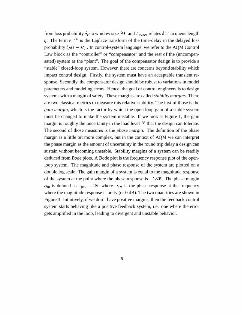
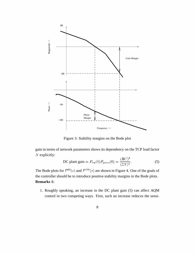
systems with a margin of safety. These margins are calledstability margins. There

are two classical metrics to measure this relative stability. The first of those is the

gain margin, which is the factor by which the open loop gain of a stable system

must be changed to make the system unstable. If we look at Figure 1, the gain

margin is roughly the uncertainty in the load levelN that the design can tolerate.

The second of those measures is thephase margin. The definition of the phase

margin is a little bit more complex, but in the context of AQM we can interpret

the phase margin as the amount of uncertainty in the round trip delay a design can

sustain without becoming unstable. Stability margins of a system can be readily

deduced fromBodeplots. A Bode plot is the frequency response plot of the open-

loop system. The magnitude and phase response of the system are plotted on a

double log scale. The gain margin of a system is equal to the magnitude response

of the system at the point where the phase response is�180o. The phase margin�m is defined as!pm � 180 where!pm is the phase response at the frequency

where the magnitude response is unity (or 0 dB). The two quantities are shown in

Figure 3. Intuitively, if we don’t have positive margins, then the feedback control

system starts behaving like a positive feedback system, i.e. one where the error

gets amplified in the loop, leading to divergent and unstablebehavior.

6

) ( s P tcp ) ( s P queue 0 sR e −

δ W δ q AQ M C o n t r o l

L a w

δ p

Figure 2:Block diagram illustrating AQM control.

2.3.1 Plant Dynamics

From Figure 2, the plant transfer function,P (s) = Pt p(s)Pqueue(s) , can be ex-

pressed in terms of network parameters yielding:Pt p(s) = R0C22N2s+ 2NR20C ;Pqueue(s) = NR0s+ 1R0 : (4)

We refer to the two poles2N=(R20C) and1=R0 aspt p andpqueue respectively.

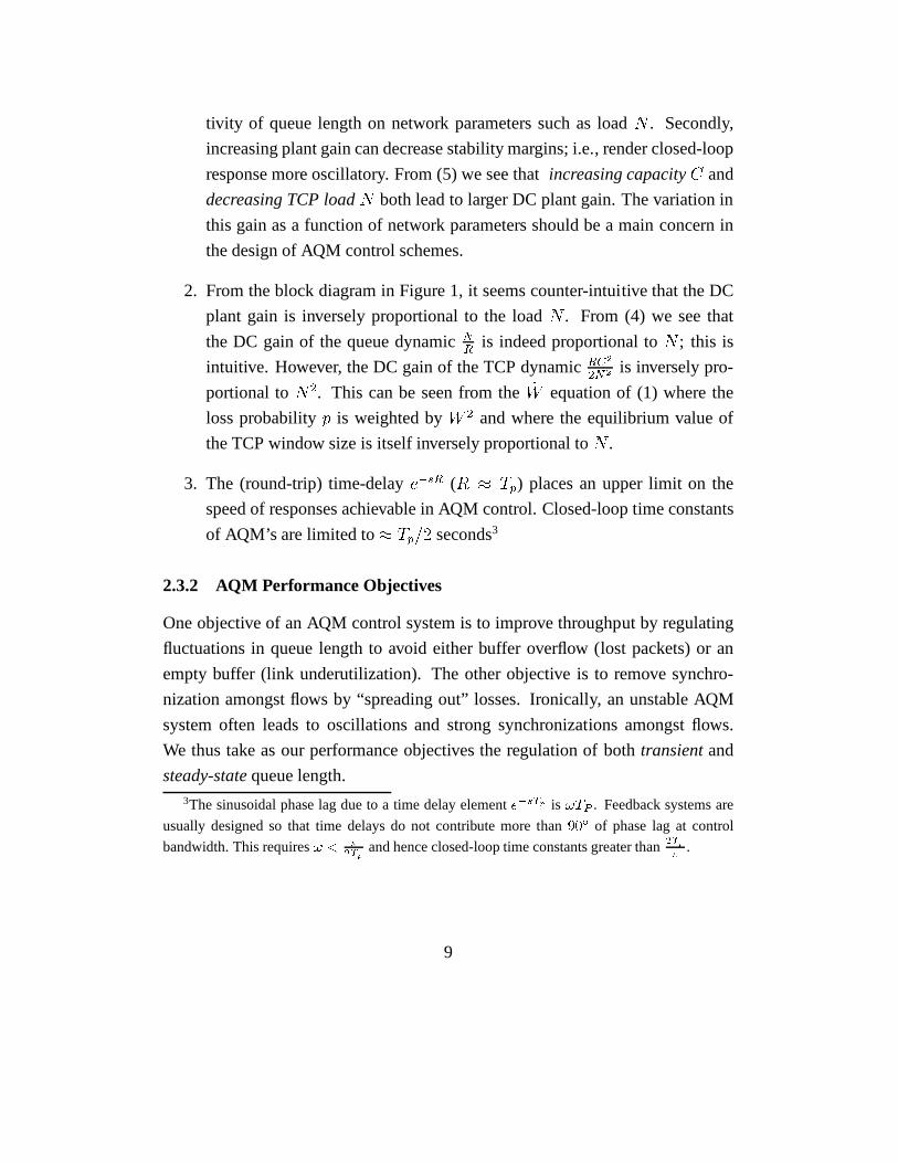
Example 1: Supposeq0 = 175 packets,Tp = 0:2 secs andC = 3750 packets/sec.

Then, for a load ofN = 60 TCP sessions, we haveW0 = 15 packets;p0 = 0:008;Pt p(s) = 482s+ 0:53; Pqueue = 243s+ 4:1;P 60(s) := Pt p(s)Pqueue(s) = 117; 126(s+ 0:53)(s+ 4:1) :For a load ofN = 120 TCP sessions, we haveW0 = 7:7; p0 = 0:034;Pt p(s) = 120s + 1:05; Pqueue = 486s+ 4:1;P 120(s) := Pt p(s)Pqueue(s) = 58; 320(s+ 1:05)(s+ 4:1) :Notice that theP 60 dynamic has larger time constants( 10:53 ; 14:1) vs. ( 11:05 ; 14:1) and

larger DC gain2, P 60(0) andP 120(0), (53; 901 vs. 13; 547). Expressing this plant2the DC gain of a system is simply it’s transfer function evaluated ats = 0, i.e., at 0 (DC)

frequency

7

−90

−180

dB

−dB

Gain Margin

PhaseMargin

Mag

nitu

de −

>P

hase

−>

Frequency −>

Figure 3: Stability margins on the Bode plot

gain in terms of network parameters shows its dependency on the TCP load factorN explicitly:

DC plant gain := Pt p(0)Pqueue(0) = (RC)3(2N)2 : (5)

The Bode plots forP 60(s) andP 120(s) are shown in Figure 4. One of the goals of

the controller should be to introduce positive stability margins in the Bode plots.

Remarks 1:

1. Roughly speaking, an increase in the DC plant gain (5) can affect AQM

control in two competing ways. First, such an increase reduces the sensi-

8

tivity of queue length on network parameters such as loadN . Secondly,

increasing plant gain can decrease stability margins; i.e., render closed-loop

response more oscillatory. From (5) we see thatincreasing capacityC and

decreasing TCP loadN both lead to larger DC plant gain. The variation in

this gain as a function of network parameters should be a mainconcern in

the design of AQM control schemes.

2. From the block diagram in Figure 1, it seems counter-intuitive that the DC

plant gain is inversely proportional to the loadN . From (4) we see that

the DC gain of the queue dynamicNR is indeed proportional toN ; this is

intuitive. However, the DC gain of the TCP dynamicRC22N2 is inversely pro-

portional toN2. This can be seen from the_W equation of (1) where the

loss probabilityp is weighted byW 2 and where the equilibrium value of

the TCP window size is itself inversely proportional toN .

3. The (round-trip) time-delaye�sR (R � Tp) places an upper limit on the

speed of responses achievable in AQM control. Closed-loop time constants

of AQM’s are limited to� Tp=2 seconds3

2.3.2 AQM Performance Objectives

One objective of an AQM control system is to improve throughput by regulating

fluctuations in queue length to avoid either buffer overflow (lost packets) or an

empty buffer (link underutilization). The other objectiveis to remove synchro-

nization amongst flows by “spreading out” losses. Ironically, an unstable AQM

system often leads to oscillations and strong synchronizations amongst flows.

We thus take as our performance objectives the regulation ofboth transientand

steady-statequeue length.3The sinusoidal phase lag due to a time delay elemente�sTp is !TP . Feedback systems are

usually designed so that time delays do not contribute more than 90Æ of phase lag at control

bandwidth. This requires! < �2Tp and hence closed-loop time constants greater than2Tp� .

9

Frequency (rad/sec)

Pha

se (

deg)

; Mag

nitu

de (

dB)

Bode Diagrams

0

20

40

60

80

100

P60 P120

10−1

100

101

102

−200

−150

−100

−50

0

To:

Y(1

)

Figure 4:Bode plots ofP (s) = Pt p(s)Pqueue(s) for TCP loads ofN = 60 andN =120.

10

3 AQM with RED

Random early detection (RED) is an AQM feedback scheme introduced in [10]. In

this section we use the previously developed linearized model of AQM to suggest

rules for tuning a RED-based controller.

3.1 Description of RED

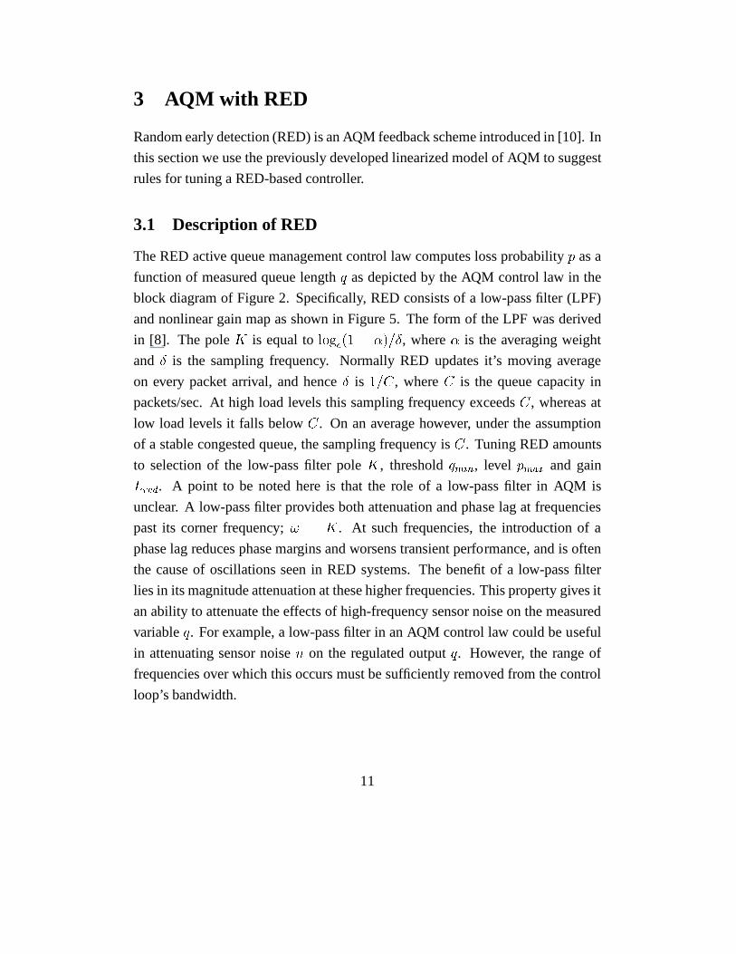
The RED active queue management control law computes loss probability p as a

function of measured queue lengthq as depicted by the AQM control law in the

block diagram of Figure 2. Specifically, RED consists of a low-pass filter (LPF)

and nonlinear gain map as shown in Figure 5. The form of the LPFwas derived

in [8]. The poleK is equal tologe(1 � �)=Æ, where� is the averaging weight

and Æ is the sampling frequency. Normally RED updates it’s movingaverage

on every packet arrival, and henceÆ is 1=C, whereC is the queue capacity in

packets/sec. At high load levels this sampling frequency exceedsC, whereas at

low load levels it falls belowC. On an average however, under the assumption

of a stable congested queue, the sampling frequency isC. Tuning RED amounts

to selection of the low-pass filter poleK, thresholdqmin, level pmax and gainLred. A point to be noted here is that the role of a low-pass filter inAQM is

unclear. A low-pass filter provides both attenuation and phase lag at frequencies

past its corner frequency;! = K. At such frequencies, the introduction of a

phase lag reduces phase margins and worsens transient performance, and is often

the cause of oscillations seen in RED systems. The benefit of alow-pass filter

lies in its magnitude attenuation at these higher frequencies. This property gives it

an ability to attenuate the effects of high-frequency sensor noise on the measured

variableq. For example, a low-pass filter in an AQM control law could be useful

in attenuating sensor noisen on the regulated outputq. However, the range of

frequencies over which this occurs must be sufficiently removed from the control

loop’s bandwidth.

11

Ks

K

+

Low-Pass FilterRED Profile

q p

p

LRED

1

minth maxth

pmax

Figure 5:RED as a cascade of low-pass filter and nonlinear gain element.

)( sResP −δq

Cδp

-(s) 0

Figure 6:Block diagram of a linearized AQM control system

3.2 Designing RED

An active queue-management (AQM) system can be modeled as the feedback

control system shown in Figure 6. HereP (s)e�sR denotes the previously derived

small-signal linearization of TCP-queue dynamics (linearized about queue-lengthq0). P (s) isPt p(s)Pqueue(s) derived previously.Æp andÆq denote perturbations in

theloss probabilityandqueue lengthrespectively. In Figure 6 the transfer functionC(s) denotes an AQM control strategy such astail-drop or RED.

Tail-drop is an on-off control strategy. In terms of our set-up in Figure 6,

tail-drop amounts to the on-off actionÆp 2 f0; 1g. It is known in control theory

that such an on-off mechanism4 leads to oscillations (limit-cycles) that can exhibit

complex and chaotic behavior; e.g., see [11]. Such oscillations may be undesirable

in queue management, and RED was introduced to stabilize them.4also referred to asrelay controlin the feedback literature.

12

A transfer-function model for RED is:C(s) = Cred(s) = Lreds=K + 1 ; (6)

where Lred = pmaxmaxth �minth ; K = loge(1� �)Æ ;� > 0 is thequeue averagingparameter andÆ is the sample time; see [8]. In de-

signingCred(s) to stabilize the AQM control system, variations in both the num-

ber of TCP sessionsN and round-trip timeR should be taken into account. The

variations inR are due to a variable propagation timeTp whereR = q0C + Tp:Let’s assume a range for the number of TCP sessions, sayN � N�, and the

round-trip time,R � R+. The objective is to select RED parametersLred andKin (6) to stabilize the linear control system in Figure 6 for all theseN andR. The

linear feedback control system in Figure 6 is stable if bounded exogenous inputs

produce only bounded outputs. This in turn implies that responses to initial con-

ditions will be bounded and converge exponentially to zero.Under this definition

of stability, we give the following two propositions:

Proposition 1: LetLred andK satisfy:Lred(R+C)3(2N�)2 � s !2gK2 + 1 (7)

where !g = 0:1min( 2N�(R+)2C ; 1R+) : (8)

Then, the linear feedback control system in Figure 6 usingC(s) = Cred(s) in (6)is stable for allN � N� and allR � R+.

Proof: Consider the frequency response of the compensated loop transfer

function L(j!) := Cred(j!)P (j!)e�j!R= Lred (RC)3(2N)2 e�j!R( j!K + 1)( j!2NR2C + 1)( j!1R + 1) :13

From this and (8) we have:L(j!) � Lred (RC)3(2N)2 e�j!Rj!K + 1 ; 8! 2 [0; !g℄:Now, given anyN � N� and anyR � R+,jL(j!g)j � Lred (R+C)3(2N�)2q !2gK2 + 1 :From this and (7) it follows thatjL(j!g)j � 1 for allN � N� and for allR � R+.

Thus, the unity-gain crossover frequency is bounded above by !g. To establish

closed-loop stability, we invoke the Nyquist stability criterion [9] and show that6 L(j!g) > �180Æ. To this end, we again use (8) to obtain6 L(j!g) � 6 Kred (R+C)3(2N�)2j!gpred + 1 � !gR � �90Æ � 0:1180� Æ > �180Æ: 2Remarks 2:

1. The rationale behind this choice of parameters is to forceCred(s) to dom-

inate closed-loop behavior. This is done by making the closed-loop time

constant (� 1=!g) greater than either the TCP time-constant(R+)2C2N� or the

queue time-constantR+.

2. Different choices of(Lred; K) satisfy the condition above. For example,

Figure 7 illustrates a region of admissible parameters5 whenR+ = 0:25secs,N� = 40, 60 and80 flows andC = 3750 packets/sec.

3. This RED design is linearly robust to the network parameter variationsN �N� andR � R+. The extent to which this feedback control system is stable

to further variations in these parameters is characterizedin Proposition 2

below.5values of admissible pairs(Lred;K) lie below the graphs.

14

10−3

10−2

0

0.5

1

1.5

2

2.5x 10

−3

K

L red

N− = 40N− = 60N− = 80

Figure 7:Stabilizing RED parametersLred andK.

15

4. The multiplicative factor0:1 in the choice of!g is the one which provides

stability margins. If we choose a higher value than0:1, we produce a con-

troller with lower stability margins. The benefit of the moreaggressive

design is that it gives faster response times (due to an increase in!g).5. It seems counter intuitive that the system is stable for all load levelsgreater

thanN�. In fact, the system may oscillate if the load level makes thesystem

go into a region where the operating point lies in the discontinuity region of

the loss profile. This was studied in [7]. However, thegentle mechanism

recommended in [12] removes the instability related to the discontinuity.

6. At high load levels, the loss probability becomes sufficiently high to cause

some flows to go into timeouts. We have ignored timeouts in ourmodel and

analysis. Timeouts should not impact stability from our analysis; indeed,

they tend to make the system less oscillatory.

Proposition 2: Consider any RED controllerCred(s) satisfying conditions(7) and (8) in Proposition 1. Then, the gain margin(GM) and phase margin(PM) of the linear control system in Figure 6 satisfy:GM � 5�; PM � 85Æ:Consequently, this linear control system will remain stable if eitherR < 15R+ orN > 15�N�.

Proof: Sharpening a phase computation made in the proof of Proposition 1

gives 6 L(j!g) � 6 Kred (R+C)3(2N�)2j!gpred + 1 � !gR � �90Æ � 0:1180� Æ � �95Æ:Thus,PM = 180Æ + 6 L(j!g) � 85Æ. The phase lag due to additional round-trip

time delay�R is: 6 e�j!g�R = �!g�R:16

From (8),!g � 0:1R . Using this and!g�R = 85( �180) gives�R � 14:8R. For the

gain margin computation we recall from the proof of Proposition 1 thatP (j!) � Lred (RC)3(2N)2j!K + 1 ; 8! 2 [0; !g℄:Consequently, 6 P (j!g) � �90Æ:Since 6 e�j!R = �90Æthen 6 L(j �2Rtt0 ) � �180Æ. BecausejL(j!g)j � 1, then1=jL(j �2Rtt0 )j � �2Rtt0!ggives a lower-bound to the gain margin. Since!g � 0:1Rtt0 thenGM � 5�: 2

Example 2: Consider the case of network parameters:C = 3750 packets/sec6, N� = 60 andR+ = 0:2 sec. From (8),!g = 0:1minf0:5259; 4:0541g = 0:053 rad/sec:ForK = 0:005, we compute from (7):Lred � (2N�)2(R+C)3s !2gK2 + 1 = 1:86e� 4:Thus, one choice forCred is Cred(s) = 1:86(10)�4s0:005 + 1 :In terms of implementation, we can break thisCred(s) down asLred = 1.86e-4; K = 0:005Now, for a link capacity of 3750pa kets=se , Æ = 2:66e � 04, yielding�, the

averaging weight, as1:33e� 6. Lred = pmax=maxth�minth. Thus, if we choosepmax as 0.1, then the dynamic range of the average queue size is approximately

17

Frequency (rad/sec)

Pha

se (

deg)

; Mag

nitu

de (

dB)

Bode Diagrams

−200

−150

−100

−50

0

50Gm=32.264 dB (at 0.98141 rad/sec), Pm=88.03 deg. (at 0.052714 rad/sec)

10−3

10−2

10−1

100

101

102

103

−1500

−1000

−500

0

Figure 8:Frequency response for loop usingCred = 9(10)�5s0:01+1 .

18

540 packets. In Figure 8 we give the Bode plot forL(j!) for N = N� andR = Rtt0+ . The phase margin =83Æ and the gain margin is79 (38dB).Remarks 3:

1. From the viewpoint ofsteady-state regulationit is desirable to selectLred in

(7) as large as possible. By steady state regulation we mean thatÆq should

go down to zero in steady state. However, under the RED mechanism the

steady state value of the queue length (for a stable system) depends upon

network conditions. ThusÆq in our linear model never goes to zero which

is not a desirable feature. We can reduce this steady state error by decreasingK. From (7),K ! 0 allowsLred !1. In this limiting case we haveCred = Kswhich corresponds to classicalintegralcompensation.

2. A drawback in using RED for stabilizing queue length is that it has a low

control-bandwidth!g which, from (8), must be less than the bandwidth of

either the queue or TCP dynamic. Consequently, closed-loopresponses are

commensurately slow7. This can be improved by introducing lead com-

pensation into RED. This results in a classical proportional-integral (PI)

compensator CPI = KPI (s=z + 1)s :The design of such a compensator is discussed in a separate companion

paper [13].

6corresponds to a 15 Mb/s link with average packet size 500 Bytes7In Example 1, the bandwidth was approximately 0.053 rad/sec. Closed-loop responses are

dominated by the associated 20-second time constant.

19

4 Simulations

We verify our propositions via simulations using thens simulator. Although our

analysis was carried out with a linearized model, the simulations are non-linear

in nature. We look at a single bottlenecked router running RED. In addition to

infinite duration, greedy flows such as the one we model, we introduce short lived,

HTTP flows into the router, to generate a more realistic traffic scenario. The HTTP

flows were simulated using the http module provided withns. The effect of flows

which are very short lived is essentially that of introducing noise to the queue. The

objective of the control system is to achieve full utilization of the bandwidth in the

presence of these short lived flows. In all our plots we depictthe time evolution

of the instantaneous queue length, with the unit of the time axis being seconds.

4.1 Experiment 1

In the first experiment, we look at a queue with 60 ftp (greedy)flows, and 180

HTTP sessions. The link bandwidth is 15 Mb/s, and the propagation delays for the

flows range uniformly between 160 and 240 ms. We attempt to control the queue

to provide a queueing delay of around 50-70 ms, and hence set theminth andmaxth of the queue as 200 and 250 respectively, with average packetsize being

500 Bytes. The averaging weight andpmax is retained as “vanilla”, i.e. the values

which are the default inns. The buffer has a maximum capacity of 800 packets.

We set thegentle parameter in RED as “on”. The instantaneous queue length

is shown in Figure 9. Observe the oscillating nature of the queue. It frequently

goes down to zero, thereby under-utilizing the link. The large oscillations also

add considerable jitter to the round trip times of the packets.

4.2 Experiment 2

Now we use the design as derived in Example 2. Thus, we set the averaging

weight to be1:33e�6, pmax to 0:1 and the dynamic range (minth; maxth) to 150-

700 packets. This should yield a stable mode of operation. The results are plotted

20

0 20 40 60 80 100 120 140 160 180 2000

100

200

300

400

500

600

Time

Que

ue S

ize

Pac

kets

/sec

Default RED paramaters

Figure 9: Experiment 1

21

in Figure 10. We indeed see that the system is stable, with small fluctuations

about an operating level of the queue. The deterministic oscillations which were

observed in the previous experiment are absent in this configuration. A point to

note however, is that it takes a long time to “settle” to the operating point. This

initialization is a major “disturbance” and one doesn’t expect to encounter it in

the normal mode of operation. However, it is related to the responsiveness of the

control system to change in operating conditions. This slowresponse is related to

a low value of!g that we use.8 We can be more aggressive in our choice of!g,to get a faster response, however that will lead to lower stability margins. In the

next experiment, we test a design which has a faster responsetime.

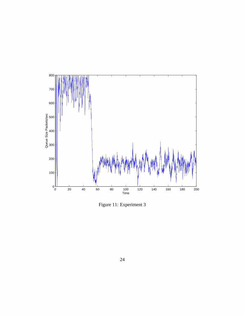
4.3 Experiment 3

We increase!g to 0.2 from 0.05. Recall that1=!g is approximately the time

constant of the feedback loop. Thus, increasing!g should yield a faster response

time. There are a number of ways of incorporating the effect of the increased!g.We look back at Proposition 1, and evaluate the effect of increasing!g onLred.We could either maintain a constant!g=K ratio, thereby increasingK (which in

turn means increasing�) and maintainLred, or we could retain the value ofK and

increaseLred correspondingly. The latter can be achieved in two different ways -

by shrinking the dynamic range (recall thatLred = pmaxmaxth�minth ) or by increasingpmax. In our first approach to obtain a faster response time, we make the dynamic

range shorter, reducing it to 150-250, from the earlier 150-700. The queue size for

this scenario is plotted in Figure 11. As we observe, the queue settles to around

the operating point after 60 seconds , compared to 80 secondsin Experiment 2.

Notice also the somewhat large deviations in the queue size around the 100-160

second range in the simulation. This is because our aggressive design has reduced

the stability margins. The presence of HTTP flows introducesa stochastic element

in the load level and hence we can expect to see those larger variations with lower8The settling time is also increased due to the non-linear effects of the tail drop phenomena

happening as the queue size reaches 800. The clamping at 800 results in a longer time for the

average to “grow” to a value which can start providing loss feedbacks

22

0 20 40 60 80 100 120 140 160 180 2000

100

200

300

400

500

600

700

800

Time

Que

ue S

ize

Pac

kets

/sec

Figure 10: Experiment 2

23

0 20 40 60 80 100 120 140 160 180 2000

100

200

300

400

500

600

700

800

Time

Que

ue S

ize

Pac

kets

/sec

Figure 11: Experiment 3

24

0 20 40 60 80 100 120 140 160 180 2000

100

200

300

400

500

600

700

800

Time

Que

ue S

ize

Pac

kets

/sec

Figure 12: Experiment 3a

stability margins.

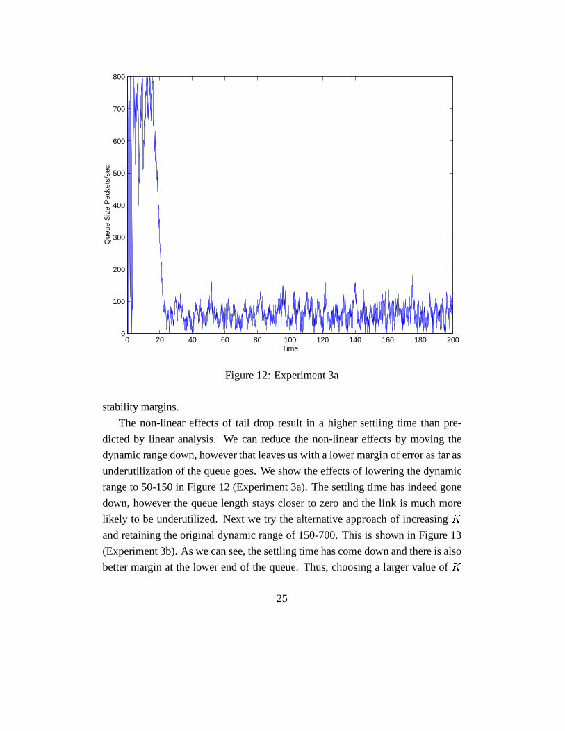
The non-linear effects of tail drop result in a higher settling time than pre-

dicted by linear analysis. We can reduce the non-linear effects by moving the

dynamic range down, however that leaves us with a lower margin of error as far as

underutilization of the queue goes. We show the effects of lowering the dynamic

range to 50-150 in Figure 12 (Experiment 3a). The settling time has indeed gone

down, however the queue length stays closer to zero and the link is much more

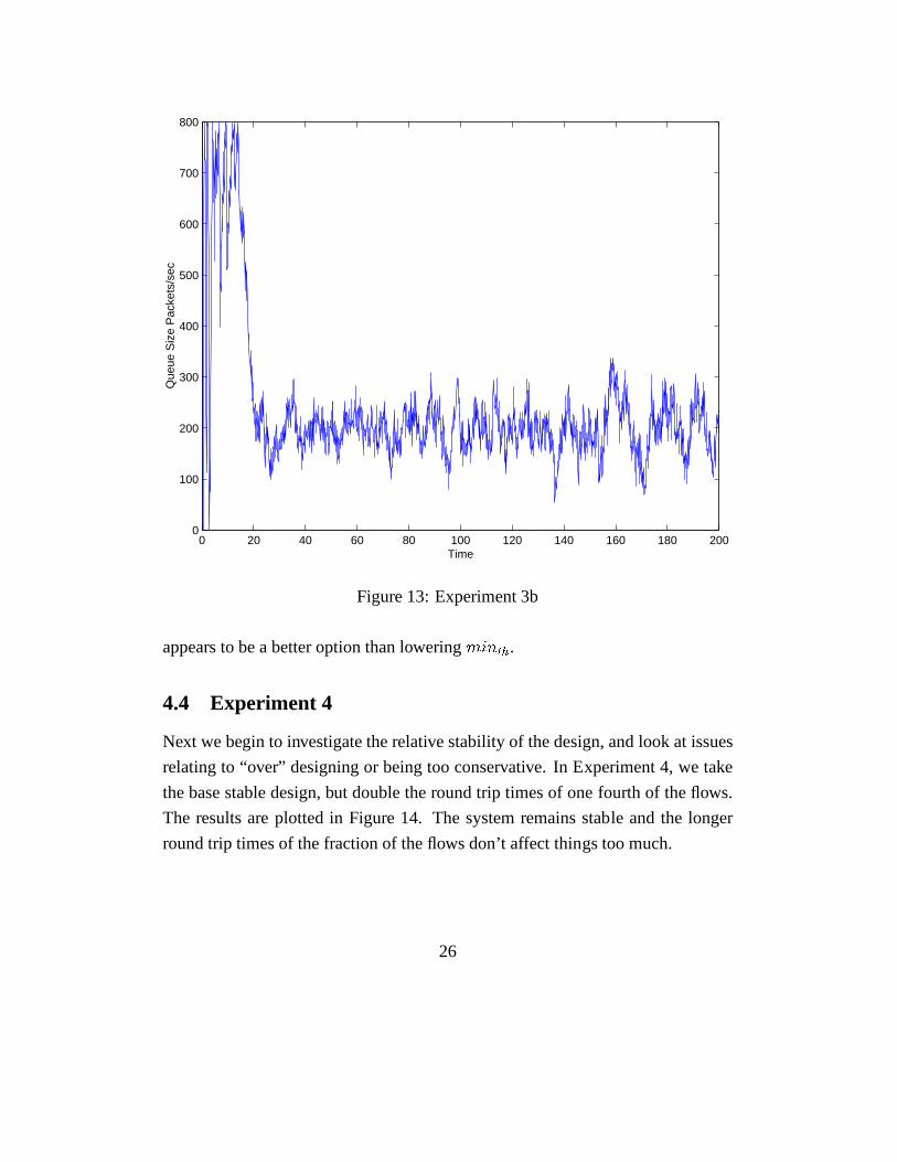
likely to be underutilized. Next we try the alternative approach of increasingKand retaining the original dynamic range of 150-700. This isshown in Figure 13

(Experiment 3b). As we can see, the settling time has come down and there is also

better margin at the lower end of the queue. Thus, choosing a larger value ofK25

0 20 40 60 80 100 120 140 160 180 2000

100

200

300

400

500

600

700

800

Time

Que

ue S

ize

Pac

kets

/sec

Figure 13: Experiment 3b

appears to be a better option than loweringminth.

4.4 Experiment 4

Next we begin to investigate the relative stability of the design, and look at issues

relating to “over” designing or being too conservative. In Experiment 4, we take

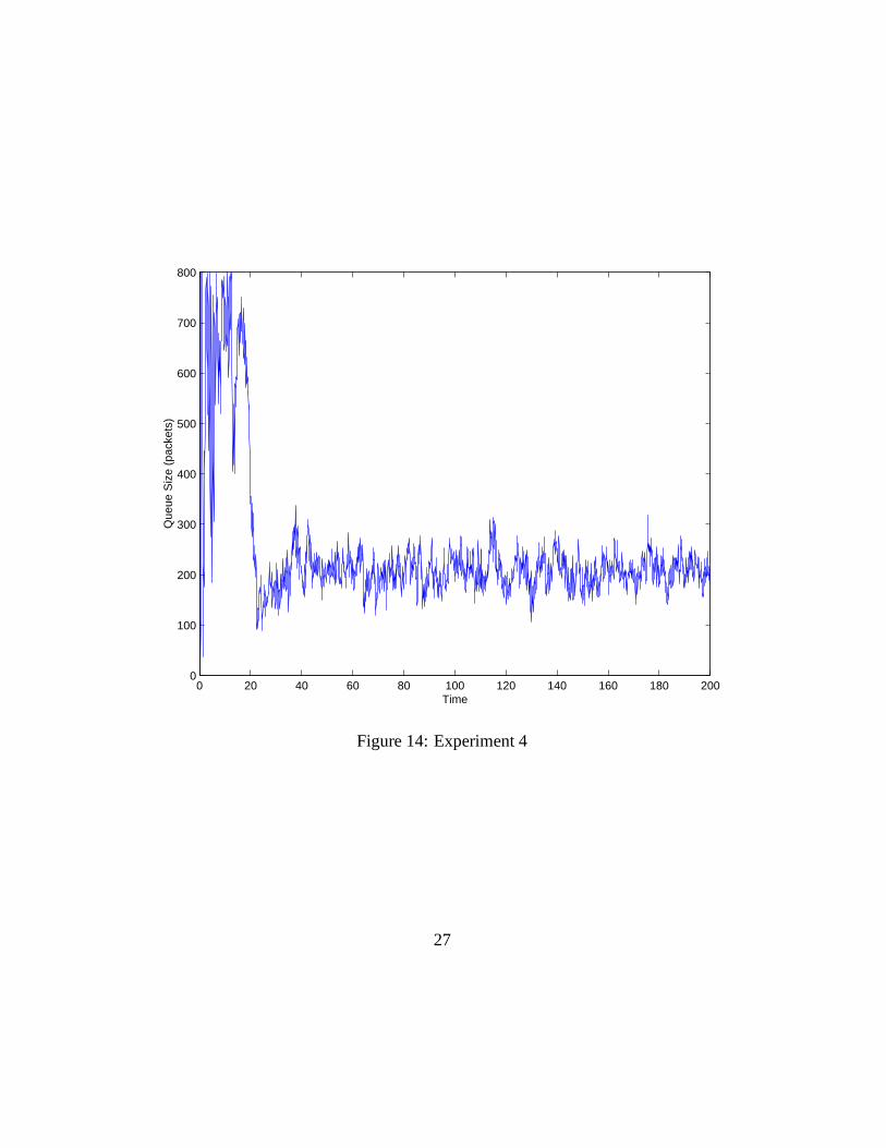
the base stable design, but double the round trip times of onefourth of the flows.

The results are plotted in Figure 14. The system remains stable and the longer

round trip times of the fraction of the flows don’t affect things too much.

26

0 20 40 60 80 100 120 140 160 180 2000

100

200

300

400

500

600

700

800

Time

Que

ue S

ize

(pac

kets

)

Figure 14: Experiment 4

27

0 20 40 60 80 100 120 140 160 180 2000

100

200

300

400

500

600

700

800

Time

Que

ue S

ize

(pac

kets

)

Figure 15: Experiment 5

4.5 Experiment 5

In this experiment, we double the round trip times ofall the flows. Thus, our sys-

tem was designed for a much lower round trip time and it shouldshow instability.

The plot is shown in Figure 15. Observe the large oscillations. One thing to take

from this experiment is that the phase margins for the non-linear system seem to

be a little lower than the ones we derived for the linear system.

4.6 Experiment 6

Now we retain the round trip time, but play around with the load level. First,

we reduce the number of ftp flows to 8. This should reduce the stability margin

28

0 20 40 60 80 100 120 140 160 180 2000

100

200

300

400

500

600

700

800

Time

Que

ue S

ize

(pac

kets

)

Figure 16: Experiment 6

according to Proposition 2. The plot in Figure 16 reveals some oscillations but the

system remains relatively stable. The gain margins in the non-linear system seem

to be retained from the linear model.

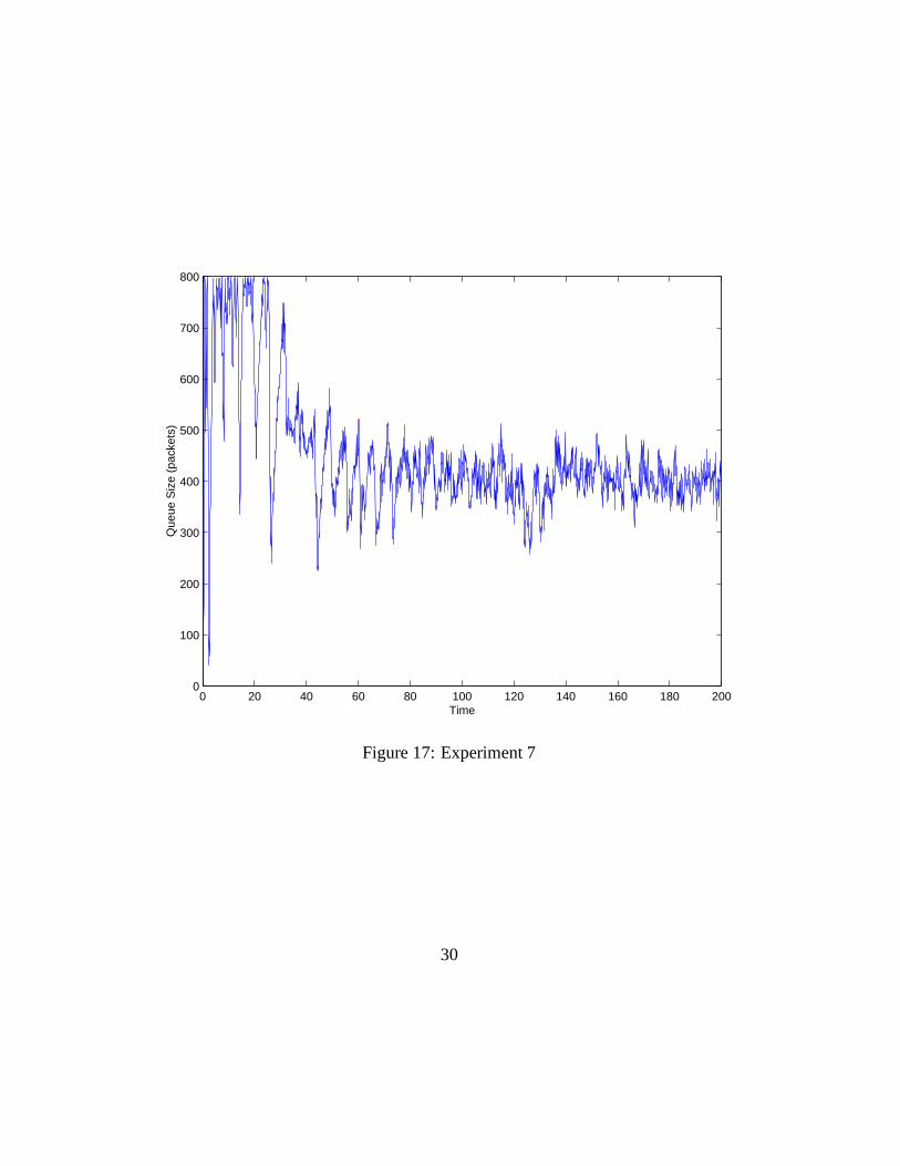
4.7 Experiment 7

Now we increase the load level. According to our analysis, the system should

remain stable, however since we have been too conservative in our design, the

performance of the compensator should be slower. Figure 17 exhibits the phe-

nomena, with the queue length taking a longer time to settle.

29

0 20 40 60 80 100 120 140 160 180 2000

100

200

300

400

500

600

700

800

Time

Que

ue S

ize

(pac

kets

)

Figure 17: Experiment 7

30

0 20 40 60 80 100 1200

100

200

300

400

500

600

700

800

Time

Que

ue S

ize

(pac

kets

)

Figure 18: Experiment 8

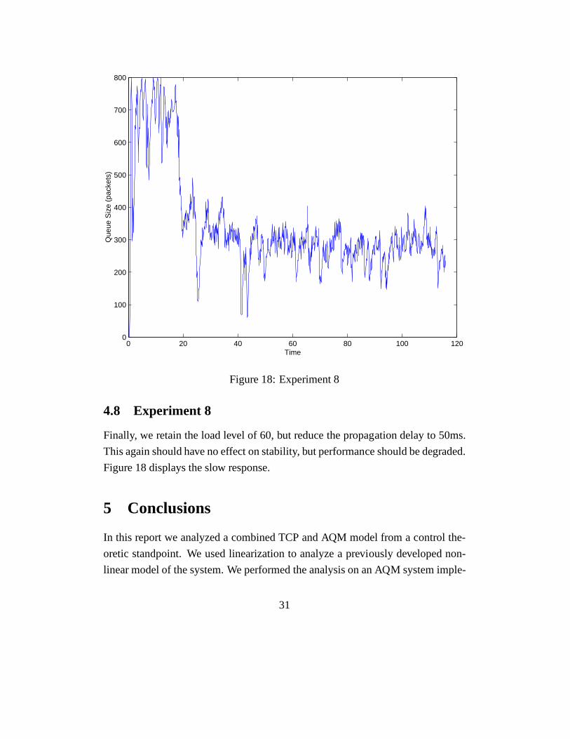
4.8 Experiment 8

Finally, we retain the load level of 60, but reduce the propagation delay to 50ms.

This again should have no effect on stability, but performance should be degraded.

Figure 18 displays the slow response.

5 Conclusions

In this report we analyzed a combined TCP and AQM model from a control the-

oretic standpoint. We used linearization to analyze a previously developed non-

linear model of the system. We performed the analysis on an AQM system imple-

31

menting RED. We are able to present design guidelines for choosing parameters

which lead to stable operation of the linear feedback control system. We are also

able to derive expressions for the relative stability of thesystem so designed. We

performed non-linear simulations usingns which verified our analysis. We are

also able to make some comments on tradeoffs of various parameter choices for

RED. In doing the analysis, we uncovered some fundamental limitations of RED.

The control theoretic model we developed points us in the direction of controllers

more suited for the particular application. There are well developed tools in classi-

cal linear system analysis which help in designing improvedcontrollers for AQM.

We are investigating those designs and they are the subject of another paper of

ours.

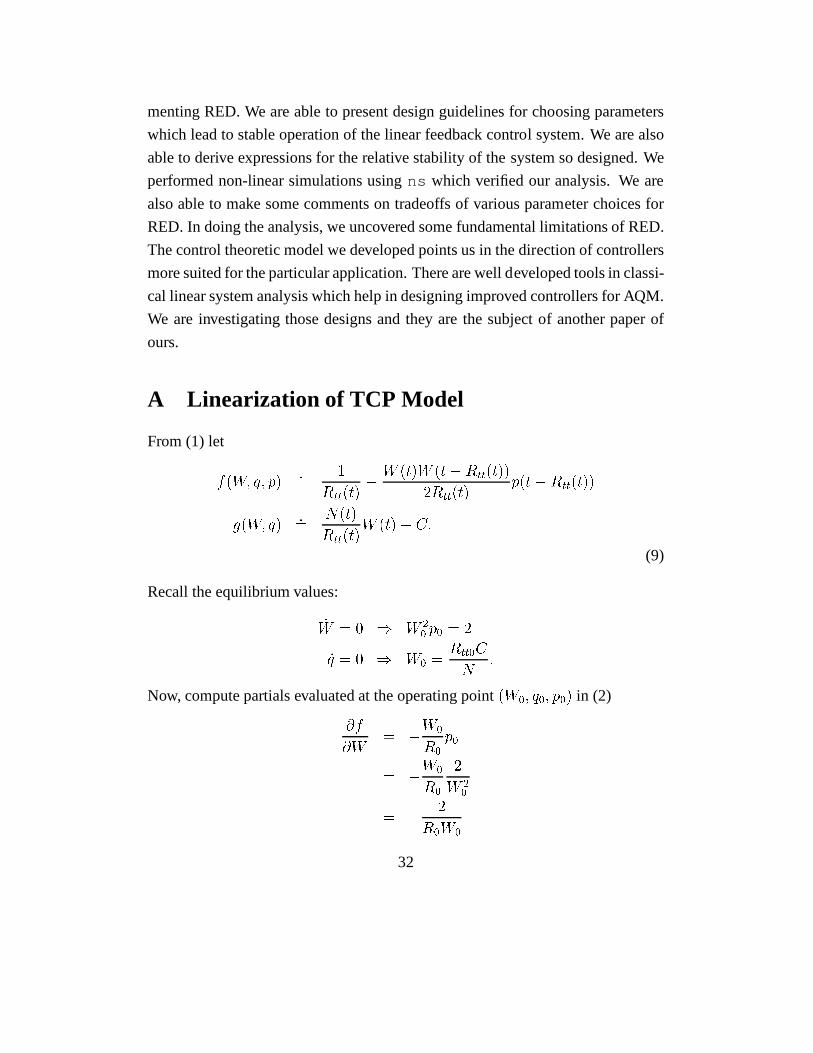
A Linearization of TCP Model

From (1) letf(W; q; p) := 1Rtt(t) � W (t)W (t� Rtt(t))2Rtt(t) p(t� Rtt(t))g(W; q) := N(t)Rtt(t)W (t)� C:(9)

Recall the equilibrium values:_W = 0 ) W 20 p0 = 2_q = 0 ) W0 = Rtt0CN :Now, compute partials evaluated at the operating point(W0; q0; p0) in (2)�f�W = �W0R0 p0= �W0R0 2W 20= � 2R0W0

32

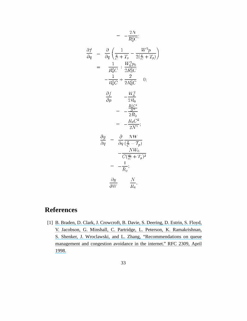
= � 2NR20C ;�f�q = ��q 1qC + Tp � W 2p2( qC + Tp)!= � 1R20C + W 20 p02R20C= � 1R20C + 22R20C = 0;�f�p = �W 202R0= � R20C2N22R0= �R0C22N2 ;�g�q = ��q NW( qC + Tp)= � NW0C( q0C + Tp)2= � 1R0 ;�g�W = NR0 :References

[1] B. Braden, D. Clark, J. Crowcroft, B. Davie, S. Deering, D. Estrin, S. Floyd,

V. Jacobson, G. Minshall, C. Partridge, L. Peterson, K. Ramakrishnan,

S. Shenker, J. Wroclawski, and L. Zhang, “Recommendations on queue

management and congestion avoidance in the internet.” RFC 2309, April

1998.

33

[2] M. C. K. Jeffay, D. Ott, and F. Smith, “Tuning Red for web traffic,” in Pro-

ceedings of ACM/SIGCOMM, 2000.

[3] M. May, T. Bonald, and J.-C. Bolot, “Analytic Evaluationof RED Perfor-

mance,” inProceedings of Infocom 2000.

[4] T. J. Ott, T. V. Lakshman, and L. H. Wong, “SRED: Stabilized RED,” in

Proceedings of Infocom 1999.

[5] W. Feng, D. Kandlur, D. Saha, and K. Shin, “Blue: A New Class of Active

Queue Management Algorithms,” tech. rep., UM CSE-TR-387-99, 1999.

[6] D. Lin and R. Morris, “Dynamics of random early detection,” in Proceedings

of ACM/SIGCOMM, 1997.

[7] V. Firoiu and M. Borden, “A study of active queue management for conges-

tion control,” inProceedings of Infocom 2000.

[8] V. Misra, W. B. Gong, and D. Towsley, “ Fluid-based Analysis of a Network

of AQM Routers Supporting TCP Flows with an Application to RED,” in

Proceedings of ACM/SIGCOMM, 2000.

[9] G. F. Franklin, J. D. Powell, and A. Emami-Naeini,Feedback Control of

Dynamic Systems. Addison-Wesley, 1995.

[10] S. Floyd and V. Jacobson, “Random Early Detection gateways for congestion

avoidance,”IEEE/ACM Transactions on Networking, vol. 1, August 1997.

[11] K. J. Astrom, “Oscillations in Systems with Relay feedback,” inAdaptive

control, filtering and signal processing, IMA Volume sin Mathematics and

its Applications, vol. 74, pp. 1–25, 1995.

[12] S. Floyd, “Recommendation on using the ”gentle” variant of RED.”

http://www.aciri.org/floyd/red/gentle.html, March 2000.

34

[13] C. Hollot, V. Misra, D. Towsley, and W. Gong, “On designing improved

controllers for AQM routers supporting TCP flows.” Submitted for review,

ftp://gaia.cs.umass.edu/pub/Misra00-AQM-Controller.ps.gz, 2000.

35