c© 2014 Meng Han

A COMPUTER VISION APPROACH FOR SEWER OVERFLOW MONITORING

BY

MENG HAN

THESIS

Submitted in partial fulfillment of the requirementsfor the degree of Master of Science in Civil Engineering

in the Graduate College of theUniversity of Illinois at Urbana-Champaign, 2014

Urbana, Illinois

Adviser:

Professor Joshua Peschel

ABSTRACT

Combined Sewer Systems (CSS) exist in over 700 communities across the United States.

Under extreme wet conditions, excess inflow which is beyond the capacity of CSS results

in Combined Sewer Overflows (CSOs); the consequence being direct discharge of untreated

water into the environment. Current CSO monitoring methods rely on in situ placement,

where the sensors are installed within the combined sewer chambers and the harsh envi-

ronment may decrease the expected lifetime of the sensors. Other limitations include high

costs and accessibility difficulties for the sensing equipment. CSOs are a major concern for

maintaining acceptable water quality standards and thus better monitoring is required.

To overcome current CSO sensing limitations, this work has created a computer vision

based approach for CSO monitoring from outlet points of CSS. This approach relies only

on video capture of CSO events at outlet points where there is flow out of a CSS, thus a

camera can be installed outside of the CSS without any contact with water. The proposed

methodology is capable of detecting, identifying and tracking CSOs by motion, shape and

color features. It is also able to measure flow rate based on a proposed model and two pro-

vided dimensions. Consequently, the approach can characterize CSOs in terms of occurrence,

duration and flow rate. In addition, the algorithm package is implemented in a Windows

desktop application for data visualization, and an iOS application for real-time CSO video

capturing and processing.

The computer vision approach was tested in a laboratory environment with three different

flow rate conditions: 5, 15 and 25 gallons per minute. The performance was evaluated

by comparing the results reported by the approach with the ground-truth baselines. The

detection of an overflow event using the computer vision approach is 1.0 second slower than a

ground-truth method. Flow rates reported by the computer vision approach are within 12%

from the ground-truth flow rate baseline. The results of this work have shown that computer

vision can be used as a reliable method for monitoring overflows under laboratory conditions.

It opens the possibility of applying computer vision techniques in CSO monitoring from

outlet points with mobile devices in the field.

ii

To my parents, for their love and support.

iii

ACKNOWLEDGMENTS

I would like to express my deepest appreciation to my adviser, Professor Joshua M. Peschel

for offering me the opportunity to be a part of this project. Without his persistent guidance

and help, this thesis would not have been possible. His advice has always kept me on the

right track. I have enjoyed working with him and I feel like I have enhanced myself a lot

throughout my master program.

I would also like to thank Dr. Sudhir Kshirsagar in Global Quality Corp. for his sup-

port and funding, also for the opportunity to let me participate in the interdisciplinary,

challenging and interesting research project.

I would like to give special thanks to my family, who always back me up when I feel

helpless. Although we are 7,000 miles away and separated by the Pacific Ocean, I could still

feel their love, care and support. And of course my girlfriend Yiwen Chen, who would like

to come to the United States for me and fulfill our dreams together.

I would not go without thanking my fellow colleagues for their encouragement and support

throughout my master program. Thank you Christopher Chini, Elizabeth Depwe, Adam

Burns, Jeff Wallace, Saki Handa and many more members in our Human Infrastructure

Interaction lab. The big family has brought me so much joy and good memories.

Thanks also go to the developers and maintainers of the open source libraries, especially

OpenCV, on which this thesis is mainly based. Also, I would like to thank many online

resources that I’ve studied from, such as Stack Overflow, iTunes University, Youtube and so

on. Thank the Information Age.

iv

TABLE OF CONTENTS

CHAPTER 1 INTRODUCTION . . . . . . . . . . . . . . . . . . . . . . . . . . . . 11.1 Research Question . . . . . . . . . . . . . . . . . . . . . . . . . . . . . . . . 11.2 Why Focus on Combined Sewer Overflows . . . . . . . . . . . . . . . . . . . 21.3 Understanding Combined Sewer Overflows . . . . . . . . . . . . . . . . . . . 21.4 Importance to Civil and Environmental Engineering . . . . . . . . . . . . . . 21.5 Contributions . . . . . . . . . . . . . . . . . . . . . . . . . . . . . . . . . . . 41.6 Organization of This Thesis . . . . . . . . . . . . . . . . . . . . . . . . . . . 5

CHAPTER 2 LITERATURE REVIEW . . . . . . . . . . . . . . . . . . . . . . . . . 62.1 Current CSO Monitoring Methods . . . . . . . . . . . . . . . . . . . . . . . . 62.2 Current Computer Vision Applications in Flow Monitoring . . . . . . . . . . 10

CHAPTER 3 METHODOLOGY . . . . . . . . . . . . . . . . . . . . . . . . . . . . 123.1 Laboratory Setup . . . . . . . . . . . . . . . . . . . . . . . . . . . . . . . . . 123.2 CSO Modeling . . . . . . . . . . . . . . . . . . . . . . . . . . . . . . . . . . . 163.3 CSO Detection . . . . . . . . . . . . . . . . . . . . . . . . . . . . . . . . . . 193.4 CSO Measurement . . . . . . . . . . . . . . . . . . . . . . . . . . . . . . . . 28

CHAPTER 4 IMPLEMENTATION . . . . . . . . . . . . . . . . . . . . . . . . . . . 324.1 Windows Desktop Application . . . . . . . . . . . . . . . . . . . . . . . . . . 324.2 iOS Application . . . . . . . . . . . . . . . . . . . . . . . . . . . . . . . . . . 34

CHAPTER 5 RESULTS . . . . . . . . . . . . . . . . . . . . . . . . . . . . . . . . . 375.1 CSO Detection . . . . . . . . . . . . . . . . . . . . . . . . . . . . . . . . . . 375.2 Occurrence . . . . . . . . . . . . . . . . . . . . . . . . . . . . . . . . . . . . 445.3 Duration . . . . . . . . . . . . . . . . . . . . . . . . . . . . . . . . . . . . . . 495.4 Flow Rate . . . . . . . . . . . . . . . . . . . . . . . . . . . . . . . . . . . . . 49

CHAPTER 6 DISCUSSION . . . . . . . . . . . . . . . . . . . . . . . . . . . . . . . 596.1 Occurrence . . . . . . . . . . . . . . . . . . . . . . . . . . . . . . . . . . . . 596.2 Duration . . . . . . . . . . . . . . . . . . . . . . . . . . . . . . . . . . . . . . 606.3 Flow Rate . . . . . . . . . . . . . . . . . . . . . . . . . . . . . . . . . . . . . 606.4 Findings . . . . . . . . . . . . . . . . . . . . . . . . . . . . . . . . . . . . . . 62

v

CHAPTER 7 CONCLUSION . . . . . . . . . . . . . . . . . . . . . . . . . . . . . . 647.1 Summary . . . . . . . . . . . . . . . . . . . . . . . . . . . . . . . . . . . . . 647.2 Limitations . . . . . . . . . . . . . . . . . . . . . . . . . . . . . . . . . . . . 657.3 Future Work . . . . . . . . . . . . . . . . . . . . . . . . . . . . . . . . . . . . 66

REFERENCES . . . . . . . . . . . . . . . . . . . . . . . . . . . . . . . . . . . . . . . 67

APPENDIX A WINDOWS APPLICATION USAGE INSTRUCTIONS . . . . . . . . 70

APPENDIX B IOS APPLICATION USAGE INSTRUCTIONS . . . . . . . . . . . . 75

vi

CHAPTER 1

INTRODUCTION

1.1 Research Question

Long-term, low-cost and accurate Combined Sewer Overflows (CSOs) monitoring is a

difficult task. Current methods to monitor CSOs usually rely on in situ sensors, including

water level sensors, temperature sensors, and flow meters. One common limitation lies in that

the sensors have to be installed inside the sewer channel and submerged by the dirty water,

thus they are not reliable and resilient enough for long-term and accurate measurement.

Moreover, the current practices cannot commonly cover all the important characteristics of

CSO, including occurrence, duration and flow rate. Even if there are flow meters that could

directly capture all required characteristics, a feasible flow meter for CSO scale measurement

could be very expensive. It is therefore necessary to develop a new low-cost method to

monitor and characterize CSO in a more reliable, economic and accurate way.

Computer vision techniques, on the other hand, has served as a feasible approach for

similar studies that are aimed for other flow monitoring, e.g. open-channel flow velocity

monitoring, river level monitoring, etc. Despite the decent performances of these studies,

similar visual sensing techniques cannot be directly applied to CSO monitoring due to the

huge differences in hydraulic features and focused characteristics.

To the best of the author’s knowledge, there are currently no long-term, low-cost and

accurate monitoring methods to characterize CSO at outlet points that exist in any urban

water infrastructure. Consequently, it is a natural progression from the current practices of

CSO monitoring and visual sensing applications in flow monitoring, to the research question

of what the appropriate visual sensing approach is for CSO monitoring and characterization.

Here, this study proposed a computer vision based approach to monitor CSOs based on

video clips captured by a smartphone or other mobile devices. The goal is to characterize

overflow in terms of occurrence, duration and flow rate at an outlet point that could be

real-time operated via a smartphone or other mobile device with a camera under lab scale

simulations.

1

1.2 Why Focus on Combined Sewer Overflows

CSO has been considered to be a major water pollution concern in approximately 772

cities in the United States that have Combined Sewer Systems (CSS) [1]. In total, CSSs

serve about 40 million people [1]. The pollutants come mostly from stormwater and untreated

human and industrial wastewater, such as untreated waste, toxic materials, and debris [1].

In addition to the severe pollution problems, CSOs usually take place in high frequency

and high volumes. Prior to 1990, the estimated annual CSO volume that was discharged to

water body in southeast Michigan was over 30 billion gallons [2]. Despite nearly 1 billion

CSO investment till 2005, there are still 10 billion gallons of CSO per year.

Given the severe consequences of CSOs, post construction monitoring becomes very nec-

essary, especially real-time monitoring. It not only allows for instant measurements to be

taken to minimize the pollution problems caused by CSOs, but also helps to understand,

model and prevent CSOs in the future.

1.3 Understanding Combined Sewer Overflows

There are mostly two kinds of sewer systems in urban systems, which are Separate Sewer

Systems and Combined Sewer Systems (CSS). In Separate Sewer Systems, stormwater runoff

is directly discharged to a receiving water body, while sanitary sewer goes to a wastewater

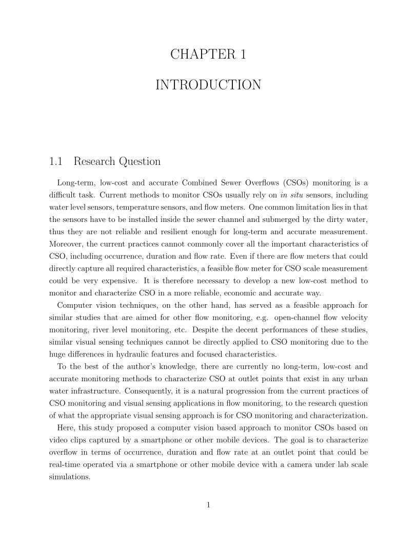
treatment plant. However, CSS as shown in Figure 1.1 receives all kinds of inflow, including

stormwater runoff, sanitary water and industrial wastewater. Under extreme wet conditions,

combined inflow that exceeds the capacity of CSS would bypass the weir wall overflow

structure and be directly discharged to a water body without treatment, resulting in a CSO

event.

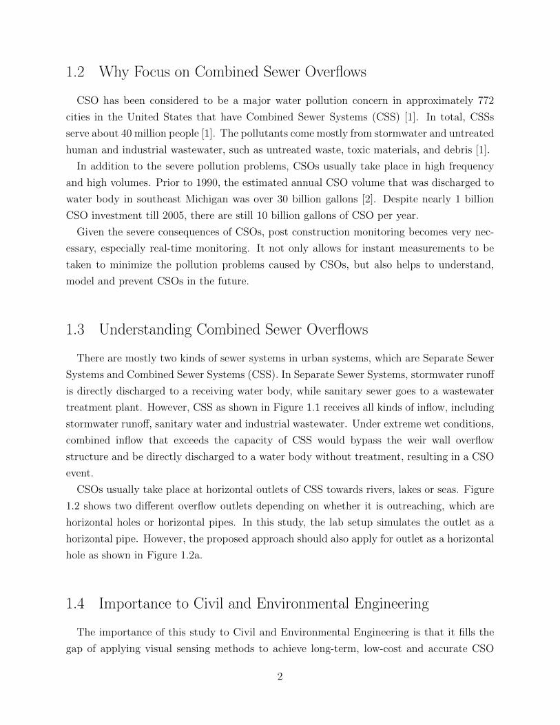
CSOs usually take place at horizontal outlets of CSS towards rivers, lakes or seas. Figure

1.2 shows two different overflow outlets depending on whether it is outreaching, which are

horizontal holes or horizontal pipes. In this study, the lab setup simulates the outlet as a

horizontal pipe. However, the proposed approach should also apply for outlet as a horizontal

hole as shown in Figure 1.2a.

1.4 Importance to Civil and Environmental Engineering

The importance of this study to Civil and Environmental Engineering is that it fills the

gap of applying visual sensing methods to achieve long-term, low-cost and accurate CSO

2

Figure 1.1: (Taken from [1]) Combined Sewer Systems bring together three maincomponents of combined sewer inflow: stormwater runoff, domestic sewage, and industrialwastewater [1]. On dry and normal wet weather conditions, CSS transports all inflow towastewater treatment facility. Treated water is then discharged to a receiving water body.However, on extreme wet weather conditions, excess flow passes weir wall overflowstructure and CSOs are discharged to a water body.

monitoring at outlet points of CSS.

To hydrologists, they would be able to better model, understand and predict CSOs with

numerical characteristics by the proposed approach in terms of occurrence, duration and

flow rate. The current CSO models could be corrected and improved with measurements. In

addition, the measurements can serve as the input parameters of CSO models for prediction.

To civil engineers, although the proposed visual sensing approach for CSO monitoring can-

not directly solve problems in other fields, they could be inspired by the idea of implementing

computer vision algorithms in portable devices to solve their problems. For instance, traffic

researchers could monitor traffic flow with similar visual sensing techniques by detecting and

tracking vehicles.

To environmental engineers, they could estimate the consequences of an CSO event with

the real-time occurrence, duration, flow rate and volume data provided by the proposed

approach. This would further allow for real-time decision making for post event treatments.

3

(a) (b)

Figure 1.2: Classification of CSS outlets. (a) CSO from horizontal holes. Horizontal holesusually come with river or lake banks. (b) CSO from horizontal pipes. The receiving waterof horizontal pipes can be rivers, lakes and seas.

1.5 Contributions

The contributions of this study are threefold. Firstly, This is the first visual sensing

implementation for automatic CSO monitoring which is focused on an outlet point of CSS.

Given that all current methods are conducted inside CSS, the sensors have to be placed

inside the harsh environment and thus the resilience of sensors are threatened. Moreover,

the installation of sensors inside CSS usually require professional sewer operators on-site.

This is the very first study that monitors CSO from the outlet points of CSS. This not only

avoids any potential contact with dirty water, but only decreases the installation efforts in

the field.

Secondly, this opens up the possibility of monitoring CSOs with just a smartphone. To

the best of the author’s knowledge, there is no current practices that utilize smartphones

to monitor CSO, instead they utilize flow meter, pressure sensor, temperature sensors, etc.

Smartphones have become more and more popular and accessible to everyone. Moreover,

the computational capabilities that a smartphone holds are already sufficient for real-time

video processing. In a sense, smartphone is a very powerful sensor with decent price.

Thirdly, this study provides a solid foundation for characterizing CSO from its motion,

shape and color features with computer vision techniques. With the proposed computer

vision based approach in this study, the overall performance in CSO monitoring is very

promising under laboratory simulations.

4

1.6 Organization of This Thesis

This thesis is organized as the following. Chapter 1 introduces the research questions

of how to appropriately monitor CSO, the importance of CSO monitoring, the cause of

CSO, and the contributions of the study. Chapter 2 presents the previous studies on how

CSOs are currently monitored and characterized, and how computer vision techniques have

been applied in similar problems. Chapter 3 presents the details of the computer vision

approach, including how the laboratory environment is set up, how videos are captured,

how CSO is modelled, and how CSO gets detected and measured, etc. Chapter 4 shows

two implementations of the algorithm package described in Chapter 3, including a Windows

desktop application and an iOS application, both called Overflow. Chapter 5 shows the

qualitative CSO detection results and quantitative results under three flow rate conditions

reported by both ground-truth baselines and proposed vision approach. Chapter 6 explains

the accuracy of the data reported by proposed vision approach in terms of occurrence,

duration and flow rate, and summarizes the findings of the study. Chapter 7 finishes with

the conclusions and findings of the research, and the suggestions for future work that is

necessary.

5

CHAPTER 2

LITERATURE REVIEW

The goal of this study is to implement computer vision based approach to monitor CSO

in terms of occurrence, duration and flow rate in a long-term, low-cost and accurate way.

The literature review is conducted on two topics that are tightly related to this study. The

first topic is about the current practices (not limited to computer vision based approach)

that have been applied in CSO monitoring in terms of occurrence, duration and flow rate.

The second topic is about the applications of computer vision based approach in flow (not

limited to CSO) monitoring.

2.1 Current CSO Monitoring Methods

CSO monitoring and characterizations, including occurrence, duration and flow rate have

been widely studied in literature and applied in real world. Based on the monitoring tech-

niques, there are three main categories of CSO monitoring methods, which are in situ sensors,

prediction models and vision based approach. In situ sensors are defined as sensors installed

within the sewer chambers in CSS. Although current computer vision based sensors were

also installed in situ, vision based approach by itself is categorized. The characterization,

strengths and weaknesses, as well as cost of each approach are analyzed respectively in this

section.

2.1.1 In situ Sensors

To monitor CSO with in situ sensors, data acquisition and data retrieval are are two

main tasks. For data acquisition, sensors of large varieties are deployed. Sensors differ from

each other based on their sensing principles, whether they are direct or indirect sensing, and

whether they are contact or non-contact with water.

Among these various in situ sensors, water level sensors, or pressure sensors are a popular

choice as deployed by [3], [4], [5], and [6]. Commercial water level sensors with water contact

6

are relatively cost-efficient, usually under $1,000, e.g. eTape Liquid Level Sensor from Milone

Technologies. However for ultrasonic water level probes, the price can easily go above $1,000,

e.g. Krohne OPTISOUND 3020 C Ultrasonic Level Gauge. The installation of water level

sensors does not require technical knowledge from sewer operators. In addition, the acquired

data can intuitively indicate whether there is CSO or not, along with the duration of CSO.

However, the accuracy of estimating flow rate is not very reliable. Although there are studies

on estimating flow rate of CSOs from water levels with computational fluid dynamics [7],

water level sensor does not work well in the case of extreme rainfall events. Moreover, the

calibration rating curve from flow depth to flow rate is a global and general hydraulic model,

which might not be able to capture local hydraulic effects [8].

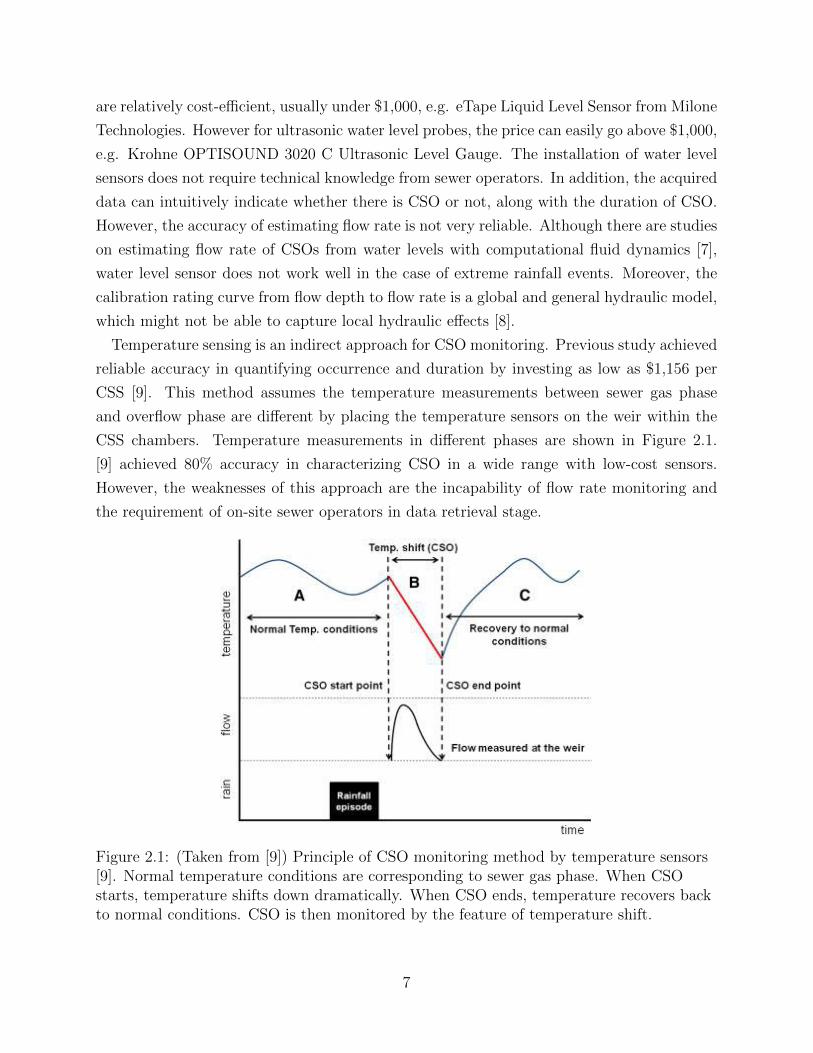
Temperature sensing is an indirect approach for CSO monitoring. Previous study achieved

reliable accuracy in quantifying occurrence and duration by investing as low as $1,156 per

CSS [9]. This method assumes the temperature measurements between sewer gas phase

and overflow phase are different by placing the temperature sensors on the weir within the

CSS chambers. Temperature measurements in different phases are shown in Figure 2.1.

[9] achieved 80% accuracy in characterizing CSO in a wide range with low-cost sensors.

However, the weaknesses of this approach are the incapability of flow rate monitoring and

the requirement of on-site sewer operators in data retrieval stage.

Figure 2.1: (Taken from [9]) Principle of CSO monitoring method by temperature sensors[9]. Normal temperature conditions are corresponding to sewer gas phase. When CSOstarts, temperature shifts down dramatically. When CSO ends, temperature recovers backto normal conditions. CSO is then monitored by the feature of temperature shift.

7

Flow meters, as a direct flow rate sensor, can characterize CSO occurrence, duration and

flow rate. However, it requires technical knowledge for sewer operators to install within the

sewer systems. In addition to the difficulty in installation, the price of flow meter usually

increases dramatically with the maximum flow rate it can measure. The sensor’s price for

measuring flow rate in CSO scale may go as high as $21,692 each [9].

For data acquisition, the installation of nearly all in situ sensors requires professional sewer

operators because sensors need to be installed within CSS. In addition to sensor installation,

sensor maintenance is often required for sensors submerged in the dirty water, requires

frequent visits by professional sewer operators.

Data retrieval is achieved in different ways. Data loggers are used to store data locally and

retrieved manually after a CSO event ([5], [9]). There are also software-based sensors that

data can be saved temporally for five minutes online from the SCADA (Supervisory Control

and Data Acquisition) system of the operator [3]. With limited space and poor network

reliability, currently there is no easy solution for retrieving data for in situ sensors remotely.

Aimed for an easy-to-implement CSO monitoring system, this study does not deploy in situ

sensors.

2.1.2 Prediction Models

CSOs are predicted by artificial neural networks based on rainfall radar data [10]. This

saves the efforts of installing any in situ sensors and achieves 95% accuracy in predicting flow

depth in the case study. However, the limitation of this approach is that it relies on rainfall

prediction accuracy because this model takes rainfall radar data as input. In addition, flow

rate can only be estimated by the flow depth predicted by this model. With a calibration

rating curve between flow rate and flow depth, the accuracy of flow rate monitoring is

expected to decrease in a non-trivial scale. Similar to [10] which predicts flow characters

by models, work in [11] uses mathematical models to estimate CSO occurrence and volume,

which also relies on rainfall data.

Although prediction models avoid lots of trouble dealing with data acquisition and data

retrieval, it is not deployed in this study because real-time flow rate accuracy is not high

enough.

8

2.1.3 Vision Based Approach

Manual visual inspection represents an intuitive way to monitor CSOs. This approach

only allows for CSO occurrence and duration monitoring, while flow rate cannot be directly

accessible, i.e. human beings can easily tell whether there is overflow or not, but are not able

to tell the exact flow rate by visual inspection. Moreover, visual inspection requires intensive

labor occupancy, which makes it unpractical for remote or long-duration monitoring.

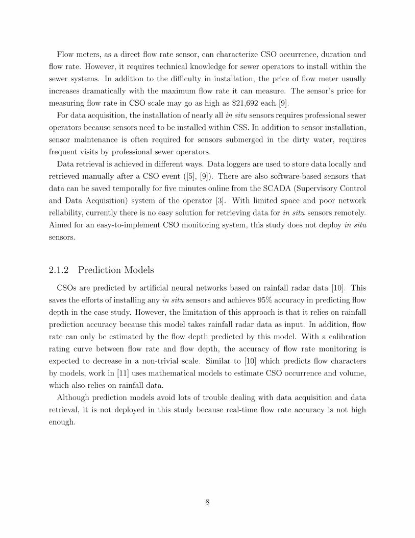
Instead of manual visual inspection, work in [8] proposed a computer vision based in

situ sensing system for automatic CSO monitoring of flow rate. A camera and an infrared

illumination device are mounted within the sewer channel with waterproof cases. The flow

velocity algorithm based on feature-based tracking is applied on the grayscale image captured

by the camera inside the sewer to calculate flow rate as shown in Figure 2.2. With its own

vision-based package as well as remote configuration, this approach requires low maintenance.

However, the weakness of this system lies in the difficulty of initial set-up in the field. To

measure real-world coordinates, the cameras need to be calibrated by a chessboard image

after the camera is mounted in the sewer to determine extrinsic parameters. This requires

technical knowledge for sewer operators. For data retrieval, the external antenna with UMTS

network is installed on-site due to the unavailability of network connectivity. This increases

the installation complexity and decreases the robustness of this system.

(a) (b) (c)

Figure 2.2: (Taken from [8]) Image analysis for particle detection [8]. (a) Original infraredimage. (b) Background estimation. (c) Binary image with possible particles for velocitymeasurement.

Vision based approach is non-contact, indirect sensing technique. The proposed approach

in this study is also based on computer vision. The main difference of the study and [8] lies

in that the camera is installed outside of the sewer system to achieve better image quality

in the daytime and to save installation efforts. Instead of capturing and tracking features in

subsequent frames captured inside CSS, the proposed approach tries to capture the features

of overflow after it flows out of the outlet points. This difference of camera placement results

9

in completely different image processing methodology as discussed in Chapter 3.

2.2 Current Computer Vision Applications in Flow Monitoring

Computer vision based approaches have been used to characterize flow velocimetry and

water level, which is applied widely in open-channel flows.

2.2.1 Velocimetry

Particle Image Velocimetry (PIV) is the most rapidly developing approach for flow velocity

measuring since its presence [12]. PIV measures the distribution of flow velocity with a high

precision. This conventional method has been modified for a large scale applications later

on [13], generally named Large Scale Particle Image Velocimetry (LSPIV). One study that

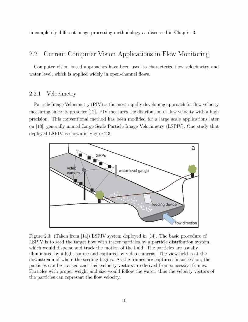
deployed LSPIV is shown in Figure 2.3.

Figure 2.3: (Taken from [14]) LSPIV system deployed in [14]. The basic procedure ofLSPIV is to seed the target flow with tracer particles by a particle distribution system,which would disperse and track the motion of the fluid. The particles are usuallyilluminated by a light source and captured by video cameras. The view field is at thedownstream of where the seeding begins. As the frames are captured in succession, theparticles can be tracked and their velocity vectors are derived from successive frames.Particles with proper weight and size would follow the water, thus the velocity vectors ofthe particles can represent the flow velocity.

10

LSPIV have been deployed by a lot of studies to characterize open-channel surface flow

velocimetry in different aspects, such as applications in shallow basins with different ge-

ometries [15], in river and dam engineering [16], in river under high flow conditions [14], in

environmental flow conditions [17], in flood discharge [18], etc. Moreover, there are studies

that combined LSPIV with numerical models to characterize flow field [17].

However, most of the vision-based approach to characterize flow are focused on open

channel surface flow. The extra particles that are used for tracing do not apply in combined

sewer overflows because of intensive existing floating waste [8]. That is the reason why PIV

based methods cannot be applied in CSO monitoring.

2.2.2 Water Level

Computer vision algorithms have also been applied in water level measurement for different

types of liquid or flow. Work in [19] proposed a computer vision based non-contact sensing

technique to measure liquid level in a closed container. It is based on establishing the

correspondence between pattern in the image and pattern in the real world. However, this

approach only applies for closed containers, instead of channel flows.

River levels have been measured by computer vision techniques ([20], [21]). In [21], bench-

marks with labels of dimensions were installed in the river and computer vision algorithms

were applied to calibrate captured images to to real-world coordinates. Although this ap-

proach achieves accurate measurement, river level has very different hydraulic features with

CSOs. Compared with rivers, the dirty water and harsh environment in CSSs, as well as

potential high flow rate of CSO make it infeasible to install benchmarks inside CSS. Conse-

quently, to capture real-world dimensions with the aid of in situ benchmarks is not deployed

in this study.

11

CHAPTER 3

METHODOLOGY

The proposed approach is described in detail within this chapter. This chapter starts

with introductions to laboratory setup and data collection. Following that, overflow rate is

mathematically modelled according to the laboratory setup. The computer vision based CSO

monitoring techniques in terms of occurrence, duration and flow rate are detailed afterwards.

3.1 Laboratory Setup

CSO laboratory setup is designed to be self-recirculated and controllable in terms of flow

rate. Figure 3.1 shows the overview of the lab setup, consisting of a horizontal pipe, a

corrugated pipe, a valve, a pump and a container.

3.1.1 Data Acquisition

An iPhone 5 device mounted on a tripod with 8-megapixel camera is used to capture

overflow videos. The original video with dimensions of 1080 × 1920 at 30 fps is then down

sampled to 480 × 854 at 5 fps. This adjustment not only allows real-time CSO monitoring

and characterization with iPhone devices, but also increases the performance of background

subtraction as discussed later. Sample frames are shown in Figure 3.2. There are four phases

in each video captured in laboratory CSO simulations: no overflow, overflow starts, steady

overflow and overflow ends.

3.1.2 Ground-truth Baseline

The results are characterized in terms of occurrence, duration and flow rate of overflow.

Ground-truth baseline of each character is determined in different ways.

12

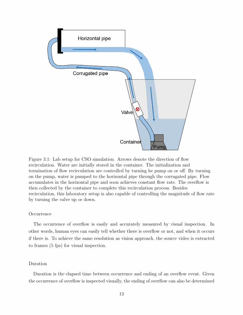
Figure 3.1: Lab setup for CSO simulation. Arrows denote the direction of flowrecirculation. Water are initially stored in the container. The initialization andtermination of flow recirculation are controlled by turning he pump on or off. By turningon the pump, water is pumped to the horizontal pipe through the corrugated pipe. Flowaccumulates in the horizontal pipe and soon achieves constant flow rate. The overflow isthen collected by the container to complete this recirculation process. Besidesrecirculation, this laboratory setup is also capable of controlling the magnitude of flow rateby turning the valve up or down.

Occurrence

The occurrence of overflow is easily and accurately measured by visual inspection. In

other words, human eyes can easily tell whether there is overflow or not, and when it occurs

if there is. To achieve the same resolution as vision approach, the source video is extracted

to frames (5 fps) for visual inspection.

Duration

Duration is the elapsed time between occurrence and ending of an overflow event. Given

the occurrence of overflow is inspected visually, the ending of overflow can also be determined

13

(a) (b) (c) (d)

Figure 3.2: Sample frames in videos captured. (a) Phase 1: no overflow. (b) Phase 2:overflow starts. (c) Phase 3: steady overflow. (d) Phase 4: overflow ends.

by human eyes. In this study, the ending of overflow is defined as the moment that water

flows out of horizontal pipe and goes down straightly. In other words, there is no horizontal

travelling distance. One example frame is shown in Figure 3.3 to demonstrate the definition

of ending of overflow in this study. Similar to occurrence baseline, the source video is

extracted to frames (5 fps) for visual inspection.

Flow Rate

An Atlas Scientific large flow meter kit is used to monitor flow rate under low flow rate

conditions (5̃ GPM), which serves as the ground-truth baseline to be compared with. The

basic information of this flow meter is listed in Table 3.1.

Table 3.1: Flow meter basic information

Product Large flow meter kit

Manufacturer Atlas ScientificRange 3.0 GPM to 30.0 GPM

As shown in Figure 3.4, pre-filter and flow meter are added before flow reaches horizontal

pipe. Flow meter is connected with a micro-controller for continuous data reading.

However, overflow monitoring in terms of flow rate by flow meter has several limitations.

Firstly, occurrence of overflow is earlier for flow meter monitoring because flow arrives at

14

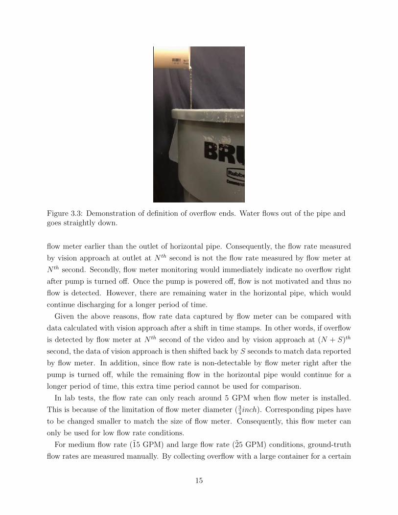
Figure 3.3: Demonstration of definition of overflow ends. Water flows out of the pipe andgoes straightly down.

flow meter earlier than the outlet of horizontal pipe. Consequently, the flow rate measured

by vision approach at outlet at N th second is not the flow rate measured by flow meter at

N th second. Secondly, flow meter monitoring would immediately indicate no overflow right

after pump is turned off. Once the pump is powered off, flow is not motivated and thus no

flow is detected. However, there are remaining water in the horizontal pipe, which would

continue discharging for a longer period of time.

Given the above reasons, flow rate data captured by flow meter can be compared with

data calculated with vision approach after a shift in time stamps. In other words, if overflow

is detected by flow meter at N th second of the video and by vision approach at (N + S)th

second, the data of vision approach is then shifted back by S seconds to match data reported

by flow meter. In addition, since flow rate is non-detectable by flow meter right after the

pump is turned off, while the remaining flow in the horizontal pipe would continue for a

longer period of time, this extra time period cannot be used for comparison.

In lab tests, the flow rate can only reach around 5 GPM when flow meter is installed.

This is because of the limitation of flow meter diameter (34inch). Corresponding pipes have

to be changed smaller to match the size of flow meter. Consequently, this flow meter can

only be used for low flow rate conditions.

For medium flow rate (1̃5 GPM) and large flow rate (2̃5 GPM) conditions, ground-truth

flow rates are measured manually. By collecting overflow with a large container for a certain

15

Figure 3.4: Laboratory set-up for flow rate measurement under low flow rate condition.Pre-filter and flow meter are added before flow reaches horizontal pipe.

period of time, flow rate can be calculated by overflow volume over time. For both flow rate

conditions, manual measurements are conducted several times for taking an average value.

Since this only records the constant flow rate after overflow has stabilized, the comparison

with vision approach can only be conducted for constant overflow period.

3.2 CSO Modeling

The modelling of CSO in the laboratory setup is based on continuity equation:

Q = vA (3.1)

where Q is the flow rate of CSO in this case, v is flow velocity, and A is wetted area in

the horizontal pipe. This model is applicable for flow that are within the horizontal pipe.

Figure 3.5 helps to illustrate the model more clearly, which excludes some components such

as the pump and pipe compared with Figure 3.1.

There are four assumptions to make for this model.

16

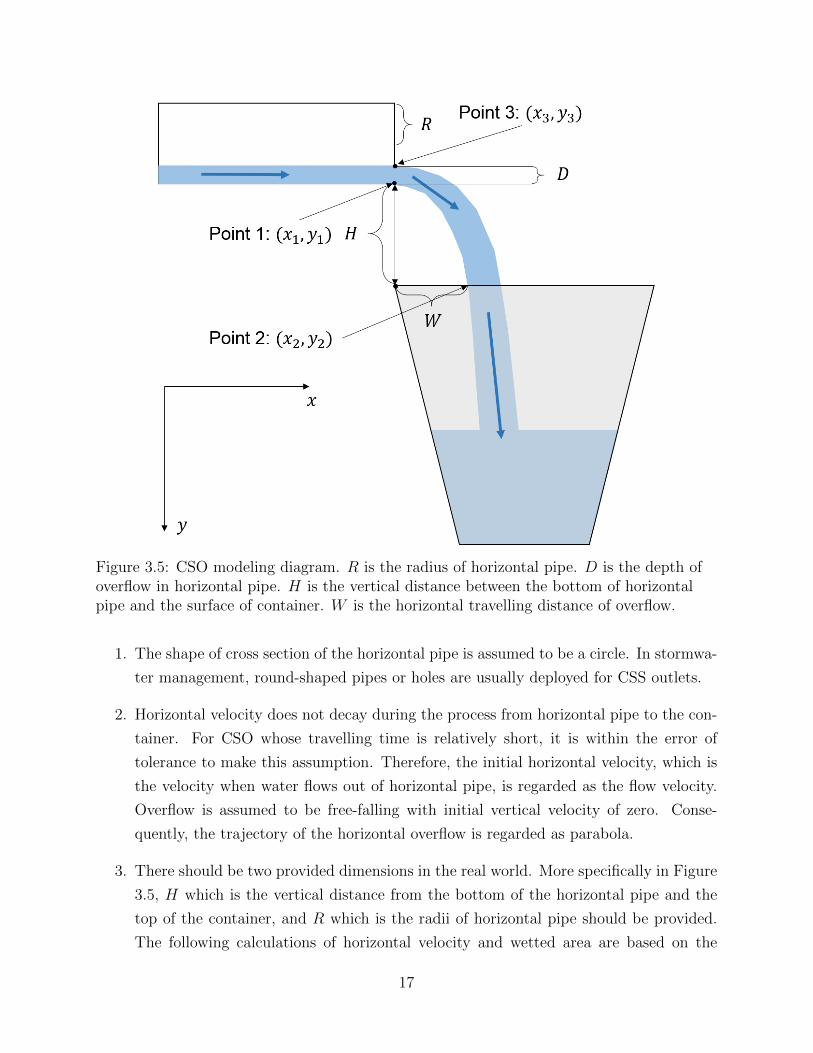
Figure 3.5: CSO modeling diagram. R is the radius of horizontal pipe. D is the depth ofoverflow in horizontal pipe. H is the vertical distance between the bottom of horizontalpipe and the surface of container. W is the horizontal travelling distance of overflow.

1. The shape of cross section of the horizontal pipe is assumed to be a circle. In stormwa-

ter management, round-shaped pipes or holes are usually deployed for CSS outlets.

2. Horizontal velocity does not decay during the process from horizontal pipe to the con-

tainer. For CSO whose travelling time is relatively short, it is within the error of

tolerance to make this assumption. Therefore, the initial horizontal velocity, which is

the velocity when water flows out of horizontal pipe, is regarded as the flow velocity.

Overflow is assumed to be free-falling with initial vertical velocity of zero. Conse-

quently, the trajectory of the horizontal overflow is regarded as parabola.

3. There should be two provided dimensions in the real world. More specifically in Figure

3.5, H which is the vertical distance from the bottom of the horizontal pipe and the

top of the container, and R which is the radii of horizontal pipe should be provided.

The following calculations of horizontal velocity and wetted area are based on the

17

assumption that H and R are provided.

4. The camera capturing angles are perpendicular to the pipe and overflow plane. In this

case, pixel distances in the frame are in scale with real-world dimensions.

Based on Equation 3.1 and the four assumptions above, flow velocity v and wetted area

in the pipe A are calculated as follows.

Suppose Point 1, 2, and 3 are three points in the captured video, the pixel distance of H

can be denoted by y2 − y1. Similarly, pixel distance of W , which is the horizontal travelling

distance of overflow, is denoted by x2 − x1. Therefore according to Assumption 4,

W = Hx2 − x1y2 − y1

(3.2)

The travelling time, t, which is the duration from flowing out of pipe and flowing into the

top of the container can be calculated as follows.

t =

√2H

g

Horizontal flow velocity, vh, remain constant according to Assumption 2. Consequently,

vht = W

vh =W

t=H x2−x1

y2−y1√2Hg

=x2 − x1y2 − y1

√gH

2(3.3)

Once the horizontal flow velocity v is determined, the next step is to calculate A, the

wetted area in the pipe. The depth of flow, D, can be denoted by pixel distances and H.

D = Hy1 − y3y2 − y1

= H(y2 − y3y2 − y1

− 1) (3.4)

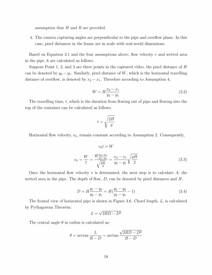
The frontal view of horizontal pipe is shown in Figure 3.6. Chord length, L, is calculated

by Pythagorean Theorem:

L =√

2RD −D2

The central angle θ in radius is calculated as:

θ = arctanL

R−D= arctan

√2RD −D2

R−D

18

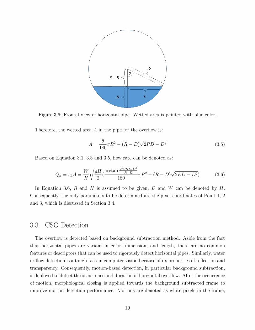
Figure 3.6: Frontal view of horizontal pipe. Wetted area is painted with blue color.

Therefore, the wetted area A in the pipe for the overflow is:

A =θ

180πR2 − (R−D)

√2RD −D2 (3.5)

Based on Equation 3.1, 3.3 and 3.5, flow rate can be denoted as:

Qh = vhA =W

H

√gH

2(arctan

√2RD−D2

R−D

180πR2 − (R−D)

√2RD −D2) (3.6)

In Equation 3.6, R and H is assumed to be given, D and W can be denoted by H.

Consequently, the only parameters to be determined are the pixel coordinates of Point 1, 2

and 3, which is discussed in Section 3.4.

3.3 CSO Detection

The overflow is detected based on background subtraction method. Aside from the fact

that horizontal pipes are variant in color, dimension, and length, there are no common

features or descriptors that can be used to rigorously detect horizontal pipes. Similarly, water

or flow detection is a tough task in computer vision because of its properties of reflection and

transparency. Consequently, motion-based detection, in particular background subtraction,

is deployed to detect the occurrence and duration of horizontal overflow. After the occurrence

of motion, morphological closing is applied towards the background subtracted frame to

improve motion detection performance. Motions are denoted as white pixels in the frame,

19

and the percentage of white pixels helps to determine whether it is motion or environment

noise. The last step is to identify CSO from other motions by its shape and color features.

3.3.1 Assumptions

There are several assumptions of motion-based detection:

1. Cameras are static while capturing videos. Any motion on camera itself would result

in detection of the whole scene. An iPhone 5 device mounted with tripod is deployed

in the lab conditions.

2. Distance from camera to overflow is in a fixed range. While the size of region of interest

on the screen is controllable by zooming in and out, distance should be controlled in a

range so that resolution would remain acceptable.

3. Overflow is not occluded by other motions or static objects.

4. There is only one overflow scene in any given video.

3.3.2 Background Subtraction

Background subtraction calculates the foreground mask performing a subtraction between

the current frame and a background model, containing the static part of the scene. Fore-

ground motion in a frame is labelled as white pixels, while static scenes remain black.

There are many available background subtraction models in OpenCV [22] and BGSLibrary

[23], each of which is designed for specific purposes. To determine which model works the

best for CSO detection, more than thirty different background subtraction models are tested

on the video captured on lab simulations. A brief comparison among three algorithms is

shown in Figure 3.7.

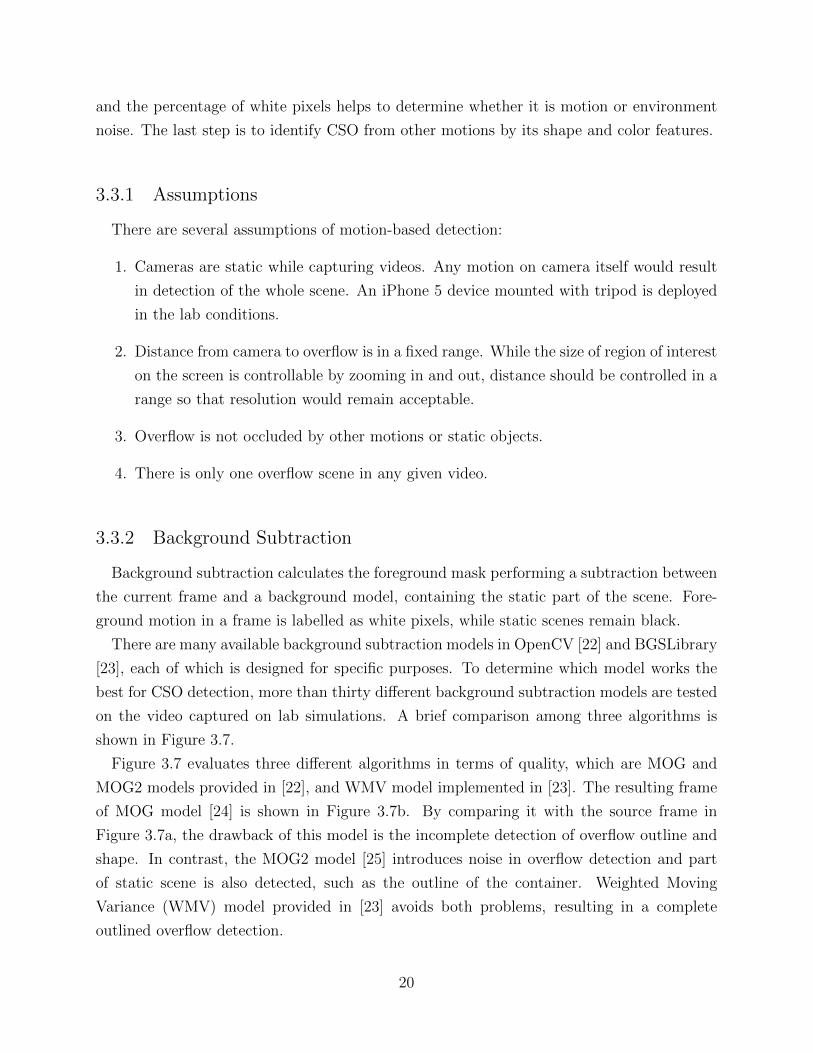
Figure 3.7 evaluates three different algorithms in terms of quality, which are MOG and

MOG2 models provided in [22], and WMV model implemented in [23]. The resulting frame

of MOG model [24] is shown in Figure 3.7b. By comparing it with the source frame in

Figure 3.7a, the drawback of this model is the incomplete detection of overflow outline and

shape. In contrast, the MOG2 model [25] introduces noise in overflow detection and part

of static scene is also detected, such as the outline of the container. Weighted Moving

Variance (WMV) model provided in [23] avoids both problems, resulting in a complete

outlined overflow detection.

20

(a) (b) (c) (d)

Figure 3.7: Performance evaluations of different background subtraction models underoverflow conditions. (a) Source frame with overflow. (b) Detected region by MOG [24]. (c)Detected region by MOG2 [25]. (d) Detected region by WMV [23].

Quality in overflow motion detection is one criteria to evaluate different background sub-

traction models. In addition, computatinoal cost is another criteria. With very similar

performance, WMV is much less computational expensive than [26] and [27] provided in

[23]. Integrating the evaluations in both quality and computational cost, WMV model is

selected as the background subtraction model for overflow detection.

WMV model calculated foreground motion in a sliding window of three consecutive frames

shown in Figure 3.8. Assume that a video consists ofN frames, sliding window moves forward

by one frame in each step. In each step, WMV model is concerned with the current frame

and its previous two frames. In addition, all frames are converted to intensity matrices with

pixel values from 0 to 1.

Assume intensity matrices of current frame and its previous two frames are denoted by

F1, F2 and F3 and their corresponding weights are w1 = 0.5, w2 = 0.3, and w3 = 0.2, then

the weighted average matrix Faver can be denoted as:

Faver = w1F1 + w2F2 + w3F3 (3.7)

In case of static scene where F1 = F2 = F3, the weighted average matrix Faver = F1.

However, in case of moving scene where current frame and its previous two frames are

mutually different, the weighted average matrix is a combination of three frames. The more

significant the motion is, the more different between three frames and average matrix are.

The next step is to determine how different they are from the average matrix by calculating

21

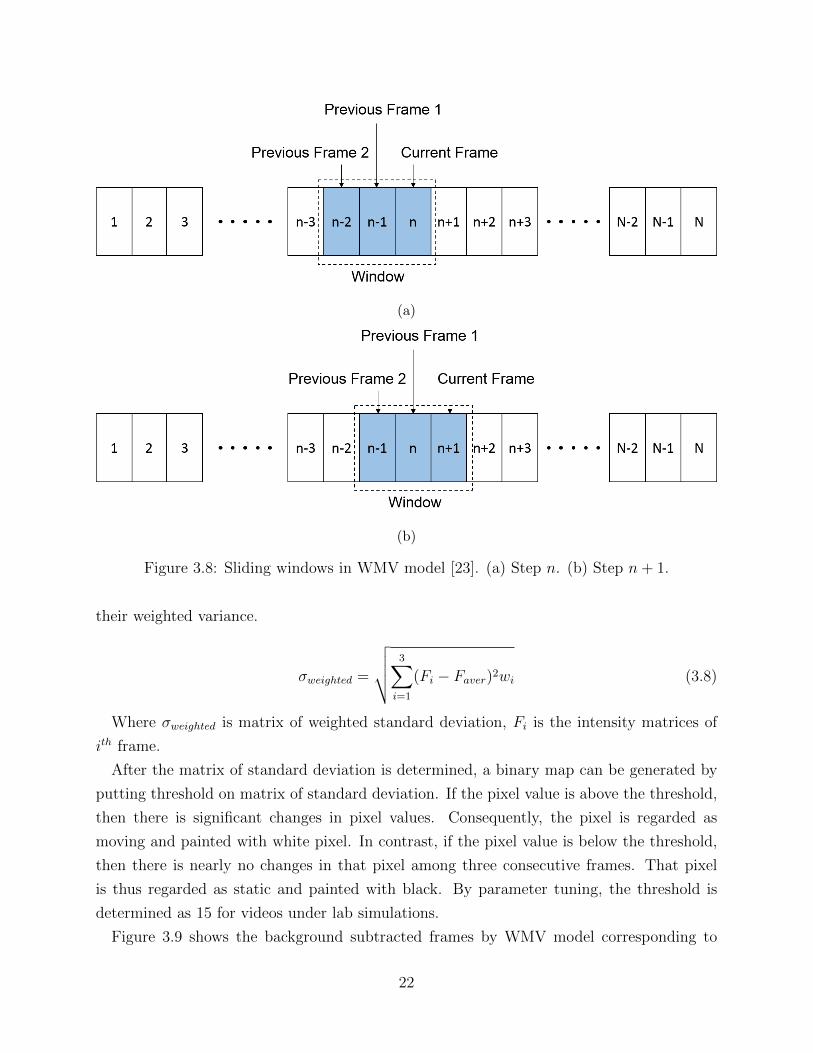
(a)

(b)

Figure 3.8: Sliding windows in WMV model [23]. (a) Step n. (b) Step n+ 1.

their weighted variance.

σweighted =

√√√√ 3∑i=1

(Fi − Faver)2wi (3.8)

Where σweighted is matrix of weighted standard deviation, Fi is the intensity matrices of

ith frame.

After the matrix of standard deviation is determined, a binary map can be generated by

putting threshold on matrix of standard deviation. If the pixel value is above the threshold,

then there is significant changes in pixel values. Consequently, the pixel is regarded as

moving and painted with white pixel. In contrast, if the pixel value is below the threshold,

then there is nearly no changes in that pixel among three consecutive frames. That pixel

is thus regarded as static and painted with black. By parameter tuning, the threshold is

determined as 15 for videos under lab simulations.

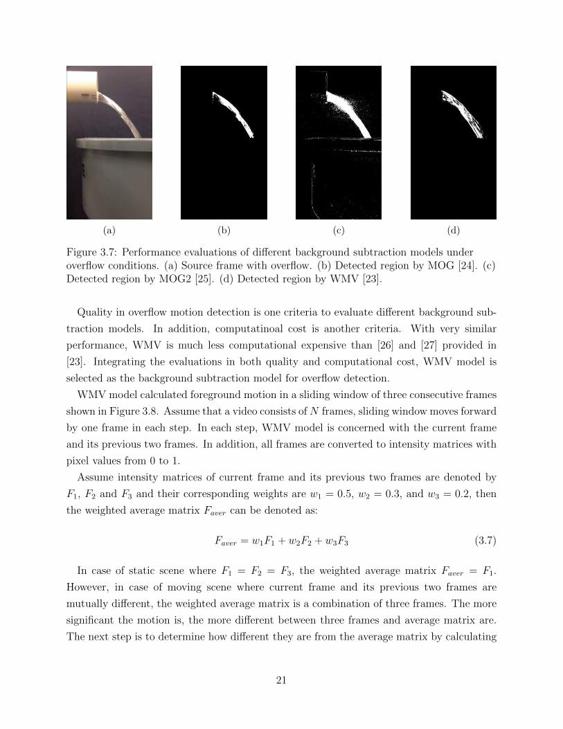
Figure 3.9 shows the background subtracted frames by WMV model corresponding to

22

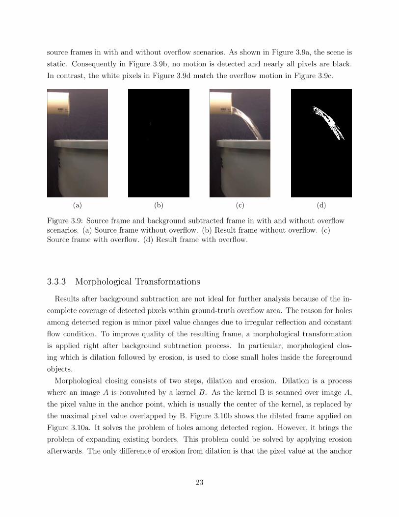
source frames in with and without overflow scenarios. As shown in Figure 3.9a, the scene is

static. Consequently in Figure 3.9b, no motion is detected and nearly all pixels are black.

In contrast, the white pixels in Figure 3.9d match the overflow motion in Figure 3.9c.

(a) (b) (c) (d)

Figure 3.9: Source frame and background subtracted frame in with and without overflowscenarios. (a) Source frame without overflow. (b) Result frame without overflow. (c)Source frame with overflow. (d) Result frame with overflow.

3.3.3 Morphological Transformations

Results after background subtraction are not ideal for further analysis because of the in-

complete coverage of detected pixels within ground-truth overflow area. The reason for holes

among detected region is minor pixel value changes due to irregular reflection and constant

flow condition. To improve quality of the resulting frame, a morphological transformation

is applied right after background subtraction process. In particular, morphological clos-

ing which is dilation followed by erosion, is used to close small holes inside the foreground

objects.

Morphological closing consists of two steps, dilation and erosion. Dilation is a process

where an image A is convoluted by a kernel B. As the kernel B is scanned over image A,

the pixel value in the anchor point, which is usually the center of the kernel, is replaced by

the maximal pixel value overlapped by B. Figure 3.10b shows the dilated frame applied on

Figure 3.10a. It solves the problem of holes among detected region. However, it brings the

problem of expanding existing borders. This problem could be solved by applying erosion

afterwards. The only difference of erosion from dilation is that the pixel value at the anchor

23

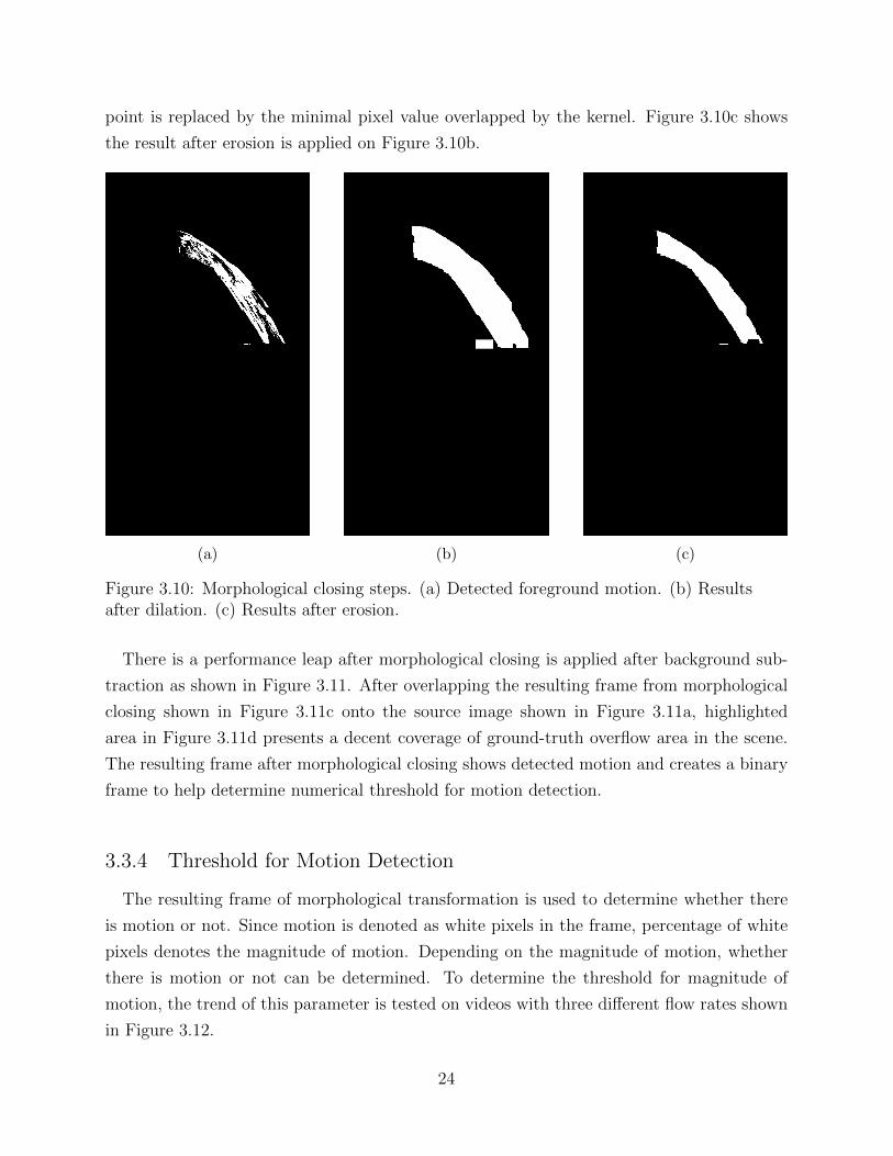
point is replaced by the minimal pixel value overlapped by the kernel. Figure 3.10c shows

the result after erosion is applied on Figure 3.10b.

(a) (b) (c)

Figure 3.10: Morphological closing steps. (a) Detected foreground motion. (b) Resultsafter dilation. (c) Results after erosion.

There is a performance leap after morphological closing is applied after background sub-

traction as shown in Figure 3.11. After overlapping the resulting frame from morphological

closing shown in Figure 3.11c onto the source image shown in Figure 3.11a, highlighted

area in Figure 3.11d presents a decent coverage of ground-truth overflow area in the scene.

The resulting frame after morphological closing shows detected motion and creates a binary

frame to help determine numerical threshold for motion detection.

3.3.4 Threshold for Motion Detection

The resulting frame of morphological transformation is used to determine whether there

is motion or not. Since motion is denoted as white pixels in the frame, percentage of white

pixels denotes the magnitude of motion. Depending on the magnitude of motion, whether

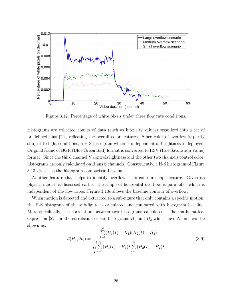
there is motion or not can be determined. To determine the threshold for magnitude of

motion, the trend of this parameter is tested on videos with three different flow rates shown

in Figure 3.12.

24

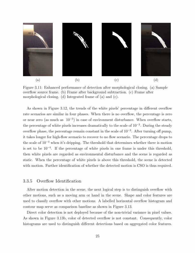
(a) (b) (c) (d)

Figure 3.11: Enhanced performance of detection after morphological closing. (a) Sampleoverflow source frame. (b) Frame after background subtraction. (c) Frame aftermorphological closing. (d) Integrated frame of (a) and (c).

As shown in Figure 3.12, the trends of the white pixels’ percentage in different overflow

rate scenarios are similar in four phases. When there is no overflow, the percentage is zero

or near zero (as much as 10−5) in case of environment disturbance. When overflow starts,

the percentage of white pixels increases dramatically to the scale of 10−3. During the steady

overflow phase, the percentage remain constant in the scale of 10−3. After turning off pump,

it takes longer for high-flow scenario to recover to no flow scenario. The percentage drops to

the scale of 10−4 when it’s dripping. The threshold that determines whether there is motion

is set to be 10−4. If the percentage of white pixels in one frame is under this threshold,

then white pixels are regarded as environmental disturbance and the scene is regarded as

static. When the percentage of white pixels is above this threshold, the scene is detected

with motion. Further identification of whether the detected motion is CSO is thus required.

3.3.5 Overflow Identification

After motion detection in the scene, the next logical step is to distinguish overflow with

other motions, such as a moving arm or hand in the scene. Shape and color features are

used to classify overflow with other motions. A labelled horizontal overflow histogram and

contour map serve as comparison baseline as shown in Figure 3.13.

Direct color detection is not deployed because of the non-trivial variance in pixel values.

As shown in Figure 3.13b, color of detected overflow is not constant. Consequently, color

histograms are used to distinguish different detections based on aggregated color features.

25

0 10 20 30 40 50 600

0.002

0.004

0.006

0.008

0.01

0.012

Video duration (second)

Per

cent

age

of w

hite

pix

els

(in d

ecim

al)

Large overflow scenarioMedium overflow scenarioSmall overflow scenario

Figure 3.12: Percentage of white pixels under three flow rate conditions.

Histograms are collected counts of data (such as intensity values) organized into a set of

predefined bins [22], reflecting the overall color features. Since color of overflow is partly

subject to light conditions, a H-S histogram which is independent of brightness is deployed.

Original frame of BGR (Blue Green Red) format is converted to HSV (Hue Saturation Value)

format. Since the third channel V controls lightness and the other two channels control color,

histograms are only calculated on H ans S channels. Consequently, a H-S histogram of Figure

3.13b is set as the histogram comparison baseline.

Another feature that helps to identify overflow is its contour shape feature. Given its

physics model as discussed earlier, the shape of horizontal overflow is parabolic, which is

independent of the flow rates. Figure 3.13c shows the baseline contour of overflow.

When motion is detected and extracted to a sub-figure that only contains a specific motion,

the H-S histogram of the sub-figure is calculated and compared with histogram baseline.

More specifically, the correlation between two histograms calculated. The mathematical

expression [22] for the correlation of two histograms H1 and H2 which have N bins can be

shown as:

d(H1, H2) =

N∑I=1

(H1(I)− H̄1)(H2(I)− H̄2)√N∑I=1

(H1(I)− H̄1)2N∑I=1

(H2(I)− H̄2)2

(3.9)

26

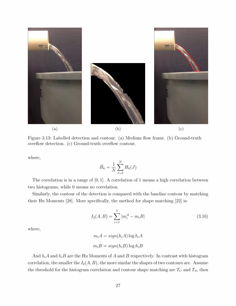
(a) (b) (c)

Figure 3.13: Labelled detection and contour. (a) Medium flow frame. (b) Ground-truthoverflow detection. (c) Ground-truth overflow contour.

where,

H̄k =1

N

N∑J=1

Hk(J)

The correlation is in a range of [0, 1]. A correlation of 1 means a high correlation between

two histograms, while 0 means no correlation.

Similarly, the contour of the detection is compared with the baseline contour by matching

their Hu Moments [28]. More specifically, the method for shape matching [22] is:

I2(A,B) =7∑

i=1

|mAi −miB| (3.10)

where,

miA = sign(hiA) log hiA

miB = sign(hiB) log hiB

And hiA and hiB are the Hu Moments of A and B respectively. In contrast with histogram

correlation, the smaller the I2(A,B), the more similar the shapes of two contours are. Assume

the threshold for the histogram correlation and contour shape matching are TC and TS, then

27

detected motion in one frame is determined as overflow only if:

d(H1, H2) > TC

I2(A,B) < TS

To better secure the reliability of identification process, the occurrence of overflow would

become true only if three consecutive frames meet the above criteria.

3.3.6 Overflow Tracking

Once overflow is identified, the next task is to track detected overflow. The algorithm

thus becomes adaptive by updating histogram baseline to keep track of overflow. More

specifically, all the motion sub-figures detected in the current frame are compared with the

histogram baseline. The sub-figures of motion with highest matching with the baseline is

labelled as overflow. Histogram baseline is then replaced with the labelled sub-figure.

Shape matching is not deployed in tracking process because of two reasons. Firstly, color

histogram comparison itself proves decent performance in overflow tracking. Secondly, this

decreases the computational cost.

3.4 CSO Measurement

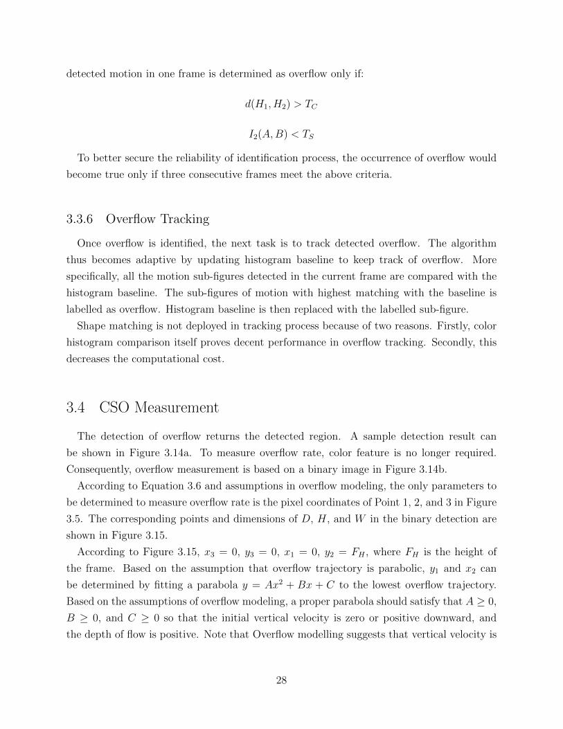
The detection of overflow returns the detected region. A sample detection result can

be shown in Figure 3.14a. To measure overflow rate, color feature is no longer required.

Consequently, overflow measurement is based on a binary image in Figure 3.14b.

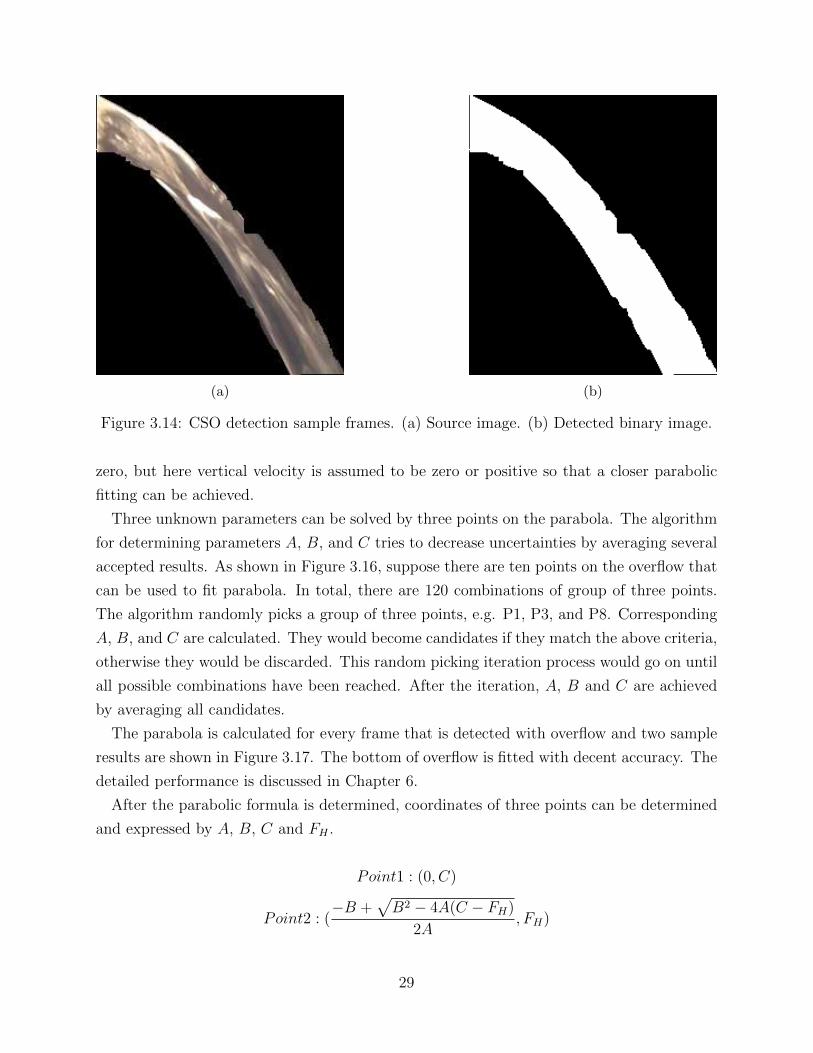
According to Equation 3.6 and assumptions in overflow modeling, the only parameters to

be determined to measure overflow rate is the pixel coordinates of Point 1, 2, and 3 in Figure

3.5. The corresponding points and dimensions of D, H, and W in the binary detection are

shown in Figure 3.15.

According to Figure 3.15, x3 = 0, y3 = 0, x1 = 0, y2 = FH , where FH is the height of

the frame. Based on the assumption that overflow trajectory is parabolic, y1 and x2 can

be determined by fitting a parabola y = Ax2 + Bx + C to the lowest overflow trajectory.

Based on the assumptions of overflow modeling, a proper parabola should satisfy that A ≥ 0,

B ≥ 0, and C ≥ 0 so that the initial vertical velocity is zero or positive downward, and

the depth of flow is positive. Note that Overflow modelling suggests that vertical velocity is

28

(a) (b)

Figure 3.14: CSO detection sample frames. (a) Source image. (b) Detected binary image.

zero, but here vertical velocity is assumed to be zero or positive so that a closer parabolic

fitting can be achieved.

Three unknown parameters can be solved by three points on the parabola. The algorithm

for determining parameters A, B, and C tries to decrease uncertainties by averaging several

accepted results. As shown in Figure 3.16, suppose there are ten points on the overflow that

can be used to fit parabola. In total, there are 120 combinations of group of three points.

The algorithm randomly picks a group of three points, e.g. P1, P3, and P8. Corresponding

A, B, and C are calculated. They would become candidates if they match the above criteria,

otherwise they would be discarded. This random picking iteration process would go on until

all possible combinations have been reached. After the iteration, A, B and C are achieved

by averaging all candidates.

The parabola is calculated for every frame that is detected with overflow and two sample

results are shown in Figure 3.17. The bottom of overflow is fitted with decent accuracy. The

detailed performance is discussed in Chapter 6.

After the parabolic formula is determined, coordinates of three points can be determined

and expressed by A, B, C and FH .

Point1 : (0, C)

Point2 : (−B +

√B2 − 4A(C − FH)

2A,FH)

29

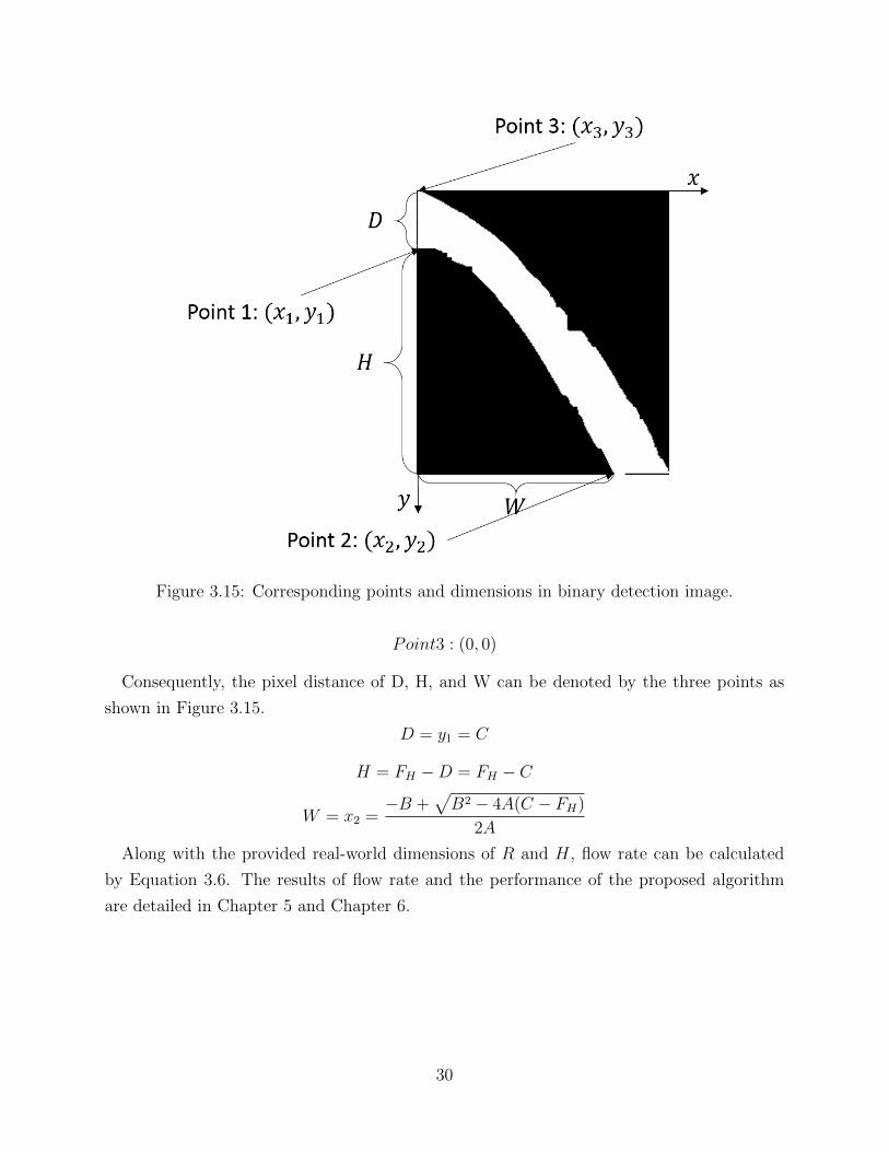
Figure 3.15: Corresponding points and dimensions in binary detection image.

Point3 : (0, 0)

Consequently, the pixel distance of D, H, and W can be denoted by the three points as

shown in Figure 3.15.

D = y1 = C

H = FH −D = FH − C

W = x2 =−B +

√B2 − 4A(C − FH)

2A

Along with the provided real-world dimensions of R and H, flow rate can be calculated

by Equation 3.6. The results of flow rate and the performance of the proposed algorithm

are detailed in Chapter 5 and Chapter 6.

30

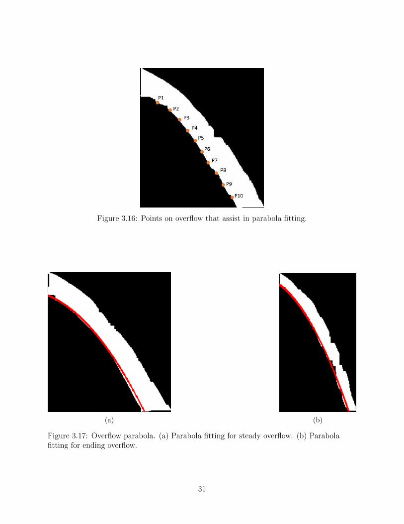
Figure 3.16: Points on overflow that assist in parabola fitting.

(a) (b)

Figure 3.17: Overflow parabola. (a) Parabola fitting for steady overflow. (b) Parabolafitting for ending overflow.

31

CHAPTER 4

IMPLEMENTATION

The methodology discussed in Chapter 3 is first implemented to an algorithm package

written in C++ based on OpenCV [22] on Ubuntu 14.04. This algorithm package is later

implemented in several platforms and devices with user interfaces designed for different

purposes. This includes Windows desktop platform and iOS, which are respectively the

most popular operation system of desktops and mobile devices [29]. Moreover, the support

with other platforms are also under consideration, such as Android and Windows Mobile

platforms.

4.1 Windows Desktop Application

There are several reasons why the algorithm package is implemented for Windows desk-

top platform. Firstly, Windows operation system is dominant in desktop operation system

market share. According to [29], Windows operation system makes up of 89% among all

desktop operation systems by September 2014. Secondly, Windows operation system and

its accessories (video player, Office Kit) dramatically increase possibilities and enhance per-

formance of presenting and analysing the resulting videos compared with the package itself.

Based on these reasons, a software for analyzing videos of CSO called Overflow, is developed

and tested on 64 bit modern Windows desktop operation systems, including Windows 7,

Windows 8 and Windows 8.1.

4.1.1 Software Development Information

The basic software development information is listed in Table 4.1.

32

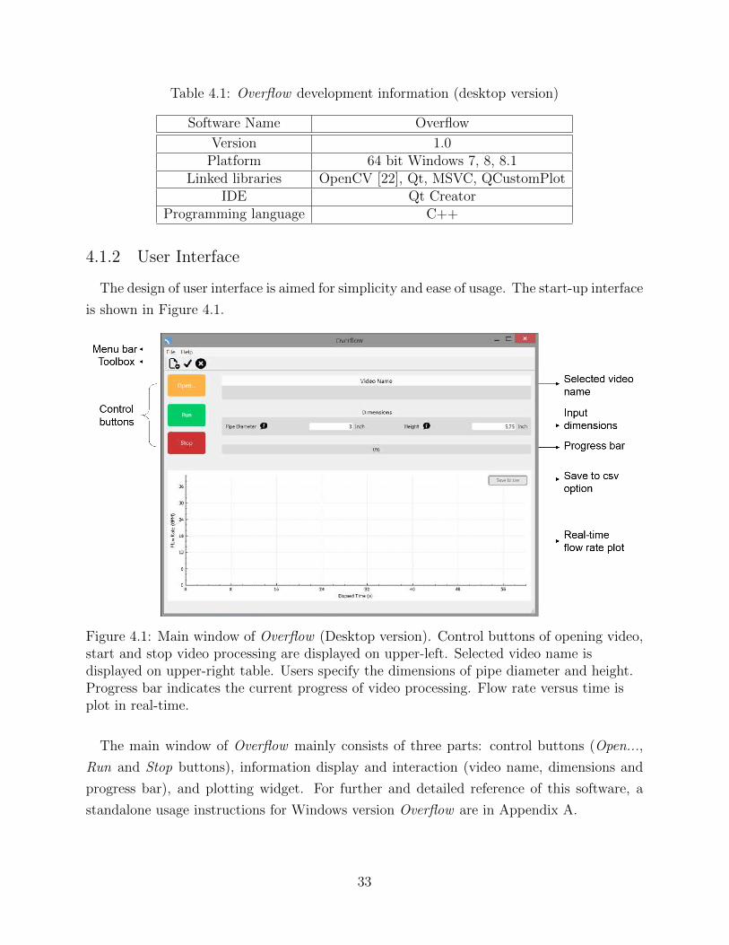
Table 4.1: Overflow development information (desktop version)

Software Name Overflow

Version 1.0Platform 64 bit Windows 7, 8, 8.1

Linked libraries OpenCV [22], Qt, MSVC, QCustomPlotIDE Qt Creator

Programming language C++

4.1.2 User Interface

The design of user interface is aimed for simplicity and ease of usage. The start-up interface

is shown in Figure 4.1.

Figure 4.1: Main window of Overflow (Desktop version). Control buttons of opening video,start and stop video processing are displayed on upper-left. Selected video name isdisplayed on upper-right table. Users specify the dimensions of pipe diameter and height.Progress bar indicates the current progress of video processing. Flow rate versus time isplot in real-time.

The main window of Overflow mainly consists of three parts: control buttons (Open...,

Run and Stop buttons), information display and interaction (video name, dimensions and

progress bar), and plotting widget. For further and detailed reference of this software, a

standalone usage instructions for Windows version Overflow are in Appendix A.

33

4.1.3 Features and Performance

The Windows desktop version of Overflow has many advantages over the back-end algo-

rithm package. Firstly, the graphical user interface makes it much easier for users without

technical knowledge to use. The operations and controls in Overflow conform with Windows

conventions and thus only minimum computer operation skills are required. Secondly, the

real-time flow rate plotting makes data visualization much better. Users can also watch the

flow rate and the video side by side and simultaneously. Thirdly, the results can be saved

for both the video and the csv file for further research.

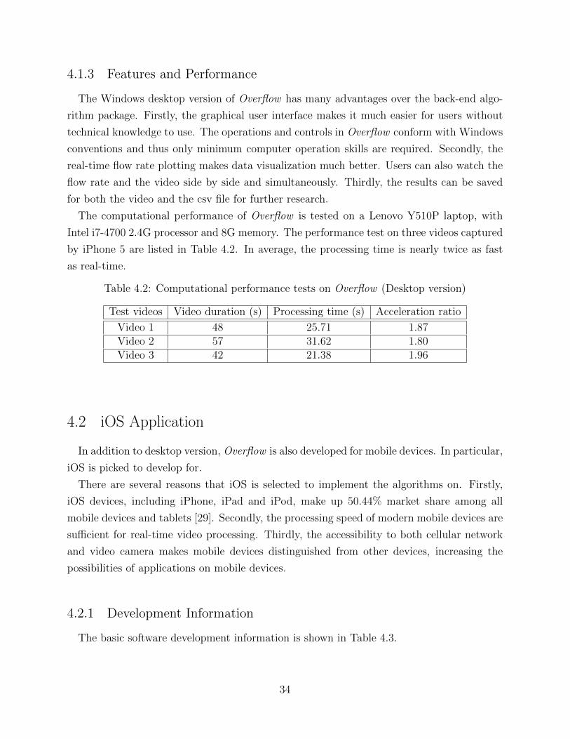
The computational performance of Overflow is tested on a Lenovo Y510P laptop, with

Intel i7-4700 2.4G processor and 8G memory. The performance test on three videos captured

by iPhone 5 are listed in Table 4.2. In average, the processing time is nearly twice as fast

as real-time.

Table 4.2: Computational performance tests on Overflow (Desktop version)

Test videos Video duration (s) Processing time (s) Acceleration ratio

Video 1 48 25.71 1.87Video 2 57 31.62 1.80Video 3 42 21.38 1.96

4.2 iOS Application

In addition to desktop version, Overflow is also developed for mobile devices. In particular,

iOS is picked to develop for.

There are several reasons that iOS is selected to implement the algorithms on. Firstly,

iOS devices, including iPhone, iPad and iPod, make up 50.44% market share among all

mobile devices and tablets [29]. Secondly, the processing speed of modern mobile devices are

sufficient for real-time video processing. Thirdly, the accessibility to both cellular network

and video camera makes mobile devices distinguished from other devices, increasing the

possibilities of applications on mobile devices.

4.2.1 Development Information

The basic software development information is shown in Table 4.3.

34

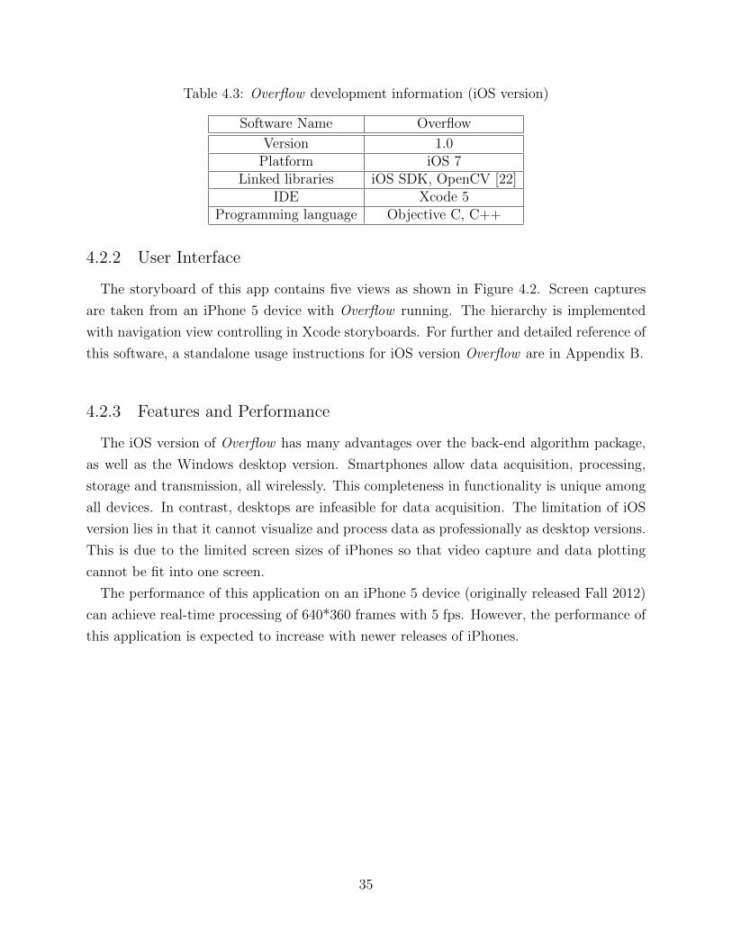
Table 4.3: Overflow development information (iOS version)

Software Name Overflow

Version 1.0Platform iOS 7

Linked libraries iOS SDK, OpenCV [22]IDE Xcode 5

Programming language Objective C, C++

4.2.2 User Interface

The storyboard of this app contains five views as shown in Figure 4.2. Screen captures

are taken from an iPhone 5 device with Overflow running. The hierarchy is implemented

with navigation view controlling in Xcode storyboards. For further and detailed reference of

this software, a standalone usage instructions for iOS version Overflow are in Appendix B.

4.2.3 Features and Performance

The iOS version of Overflow has many advantages over the back-end algorithm package,

as well as the Windows desktop version. Smartphones allow data acquisition, processing,

storage and transmission, all wirelessly. This completeness in functionality is unique among

all devices. In contrast, desktops are infeasible for data acquisition. The limitation of iOS

version lies in that it cannot visualize and process data as professionally as desktop versions.

This is due to the limited screen sizes of iPhones so that video capture and data plotting

cannot be fit into one screen.

The performance of this application on an iPhone 5 device (originally released Fall 2012)

can achieve real-time processing of 640*360 frames with 5 fps. However, the performance of

this application is expected to increase with newer releases of iPhones.

35

(a) (b) (c)

(d) (e)

Figure 4.2: Overflow storyboard (iOS version). (a) View 1: Homepage. Request user inputof dimensions of R and H. (b) View 2: About. Display overview and development team ofOverflow. (c) View 3: Video Processing. Video capture, processing and controls areincluded. (d) View 4: Display results and options to save and send the result. (e) View 5:Send file of flow rate through Email.

36

CHAPTER 5

RESULTS

The proposed approach is tested under laboratory simulations as shown in Figure 3.1.

Qualitative CSO detection results and quantitative results of occurrence, duration and flow

rate reported by proposed vision approach and ground-truth baselines are shown in this

chapter. The required parameters corresponding to Figure 3.5 are shown in Table 5.1.

Table 5.1: Dimensions of parameters under laboratory simulations

Parameters Dimensions (inch)

H 5.5R 1.5

5.1 CSO Detection

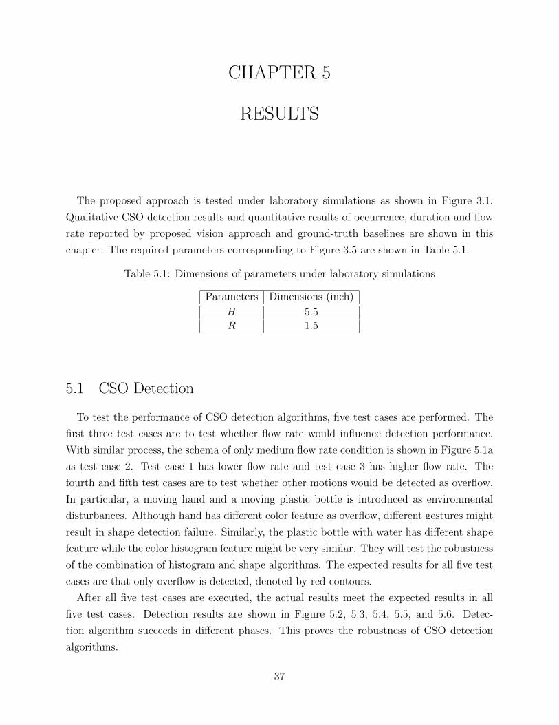
To test the performance of CSO detection algorithms, five test cases are performed. The

first three test cases are to test whether flow rate would influence detection performance.

With similar process, the schema of only medium flow rate condition is shown in Figure 5.1a

as test case 2. Test case 1 has lower flow rate and test case 3 has higher flow rate. The

fourth and fifth test cases are to test whether other motions would be detected as overflow.

In particular, a moving hand and a moving plastic bottle is introduced as environmental

disturbances. Although hand has different color feature as overflow, different gestures might

result in shape detection failure. Similarly, the plastic bottle with water has different shape

feature while the color histogram feature might be very similar. They will test the robustness

of the combination of histogram and shape algorithms. The expected results for all five test

cases are that only overflow is detected, denoted by red contours.

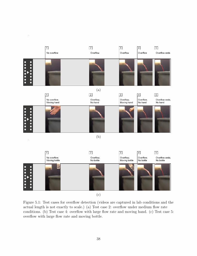
After all five test cases are executed, the actual results meet the expected results in all

five test cases. Detection results are shown in Figure 5.2, 5.3, 5.4, 5.5, and 5.6. Detec-

tion algorithm succeeds in different phases. This proves the robustness of CSO detection

algorithms.

37

(a)

(b)

(c)

Figure 5.1: Test cases for overflow detection (videos are captured in lab conditions and theactual length is not exactly to scale.) (a) Test case 2: overflow under medium flow rateconditions. (b) Test case 4: overflow with large flow rate and moving hand. (c) Test case 5:overflow with large flow rate and moving bottle.

38

(a) (b) (c) (d)

(e) (f) (g) (h)

Figure 5.2: Results of test case 1 for overflow detection. (a)(b) No overflow. Nothing isdetected. (c)(d)(e)(f)(g) Overflow initializes and stabilizes. Overflow is detected correctly.(h) Overflow continues to be detected correctly as it decays.

39

(a) (b) (c) (d)

(e) (f) (g) (h)

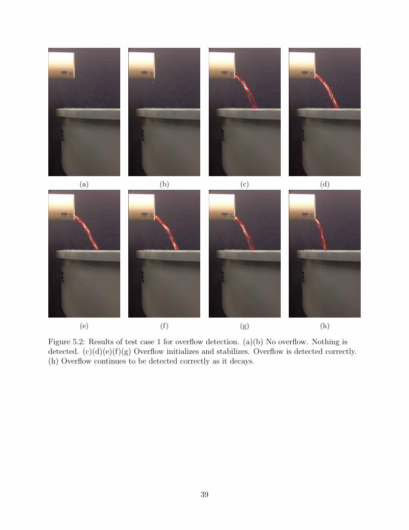
Figure 5.3: Results of test case 2 for overflow detection. (a) No overflow. Nothing isdetected. (b)(c)(d)(e) Overflow initializes and stabilizes. Overflow is detected correctly.(f)(g)(h) Overflow continues to be detected correctly as it decays.

40

(a) (b) (c) (d)

(e) (f) (g) (h)

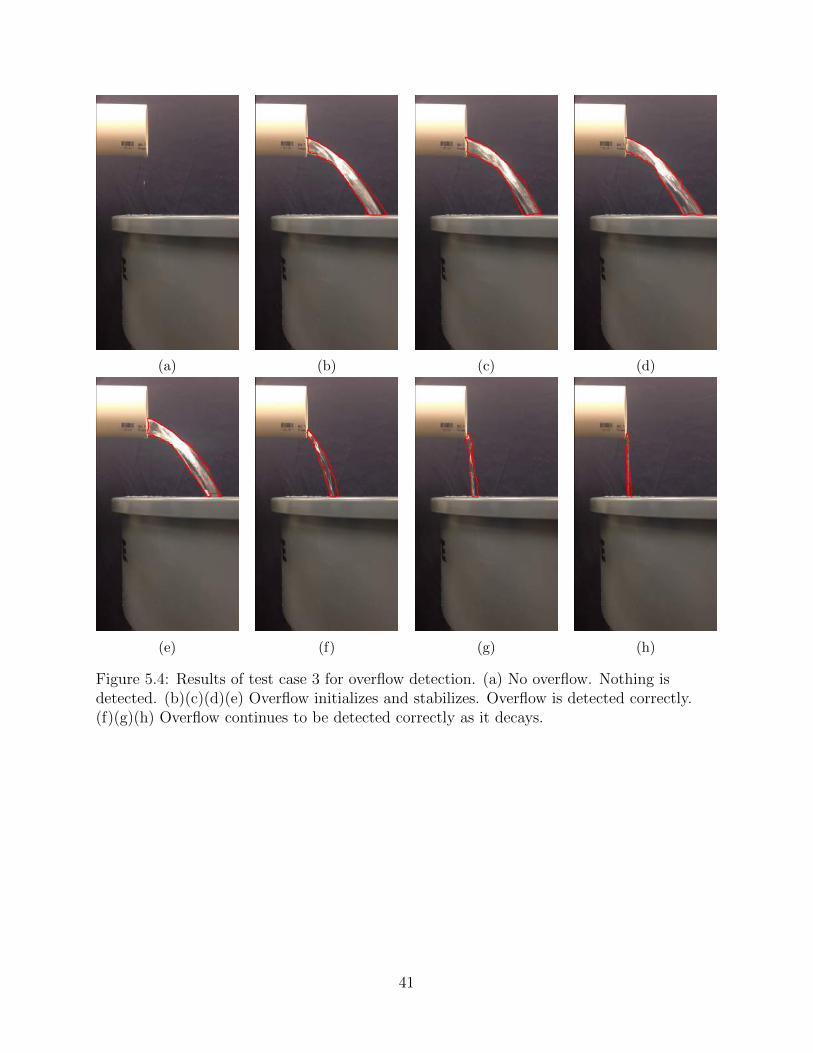
Figure 5.4: Results of test case 3 for overflow detection. (a) No overflow. Nothing isdetected. (b)(c)(d)(e) Overflow initializes and stabilizes. Overflow is detected correctly.(f)(g)(h) Overflow continues to be detected correctly as it decays.

41

(a) (b) (c) (d)

(e) (f) (g) (h)

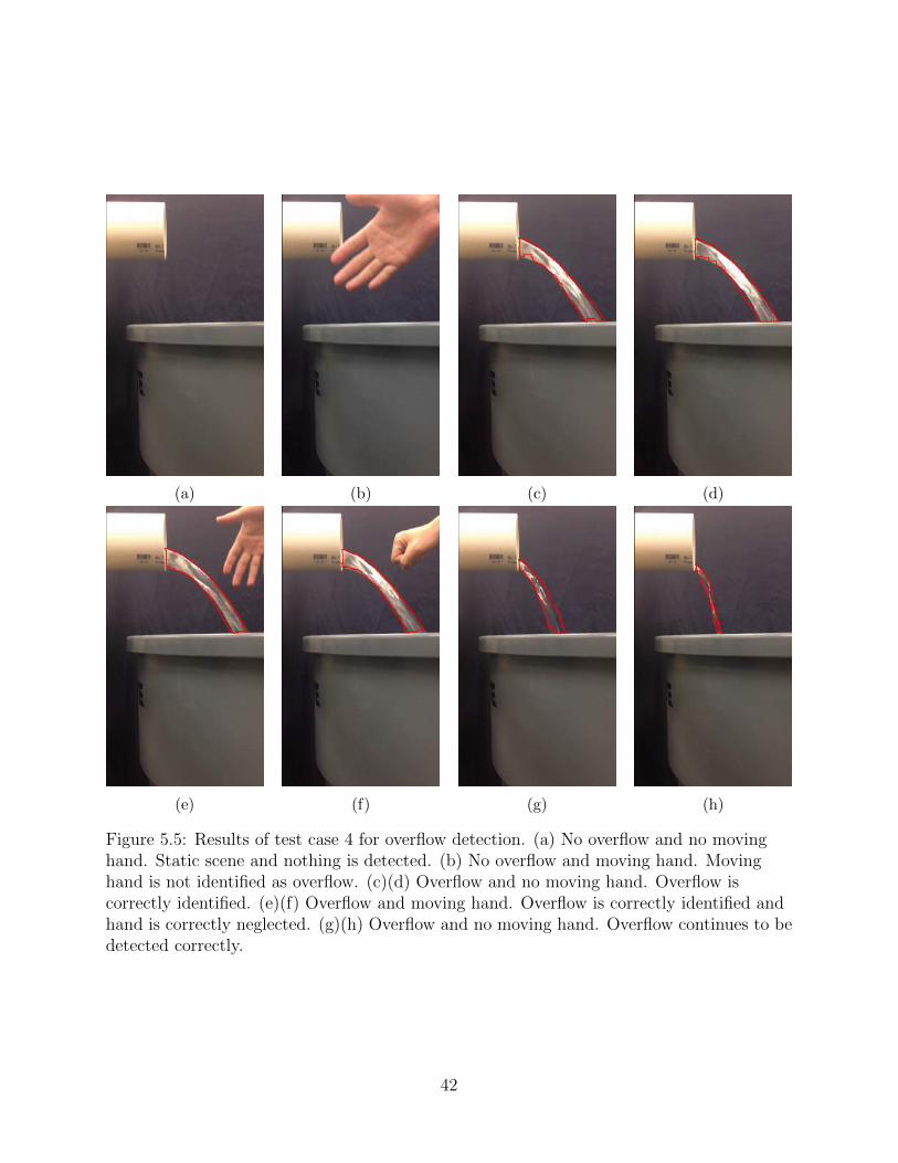
Figure 5.5: Results of test case 4 for overflow detection. (a) No overflow and no movinghand. Static scene and nothing is detected. (b) No overflow and moving hand. Movinghand is not identified as overflow. (c)(d) Overflow and no moving hand. Overflow iscorrectly identified. (e)(f) Overflow and moving hand. Overflow is correctly identified andhand is correctly neglected. (g)(h) Overflow and no moving hand. Overflow continues to bedetected correctly.

42

(a) (b) (c) (d)

(e) (f) (g) (h)

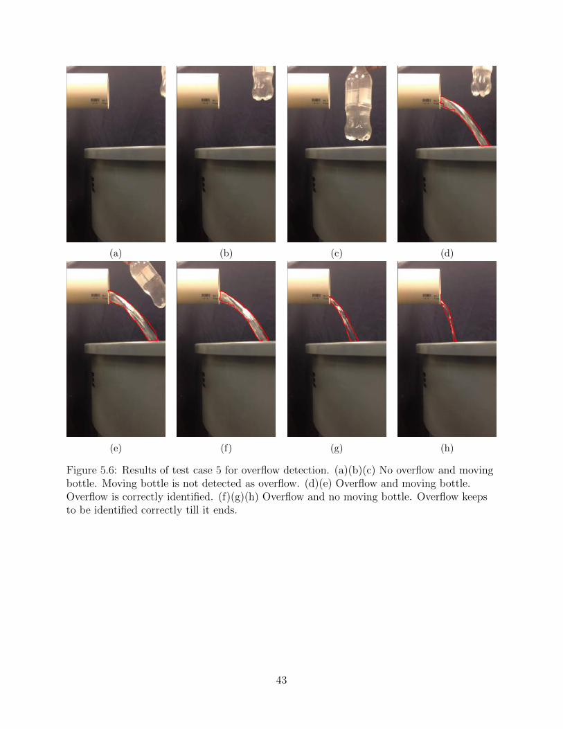
Figure 5.6: Results of test case 5 for overflow detection. (a)(b)(c) No overflow and movingbottle. Moving bottle is not detected as overflow. (d)(e) Overflow and moving bottle.Overflow is correctly identified. (f)(g)(h) Overflow and no moving bottle. Overflow keepsto be identified correctly till it ends.

43

5.2 Occurrence

The proposed approach is tested on another three flow rate conditions for occurrence,

duration and flow rate. An approximately two-minute video is captured for each flow rate

condition. No environmental disturbances are introduced in this test cases since the detection

performance has been proved to be robust in previous section. The basic procedure of the

videos is:

1. No overflow. Static screen for a certain period of time.

2. Overflow starts and stabilizes. Pump is turned on and overflow starts. The pump

keeps running for more than one minute.

3. Overflow ends. Pump is turned off and overflow begins to decay. Eventually overflow

ends.

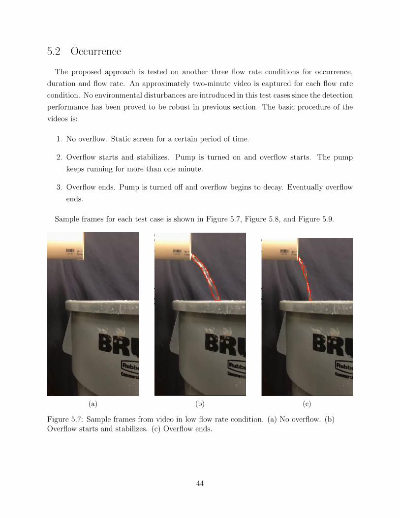
Sample frames for each test case is shown in Figure 5.7, Figure 5.8, and Figure 5.9.

(a) (b) (c)

Figure 5.7: Sample frames from video in low flow rate condition. (a) No overflow. (b)Overflow starts and stabilizes. (c) Overflow ends.

44

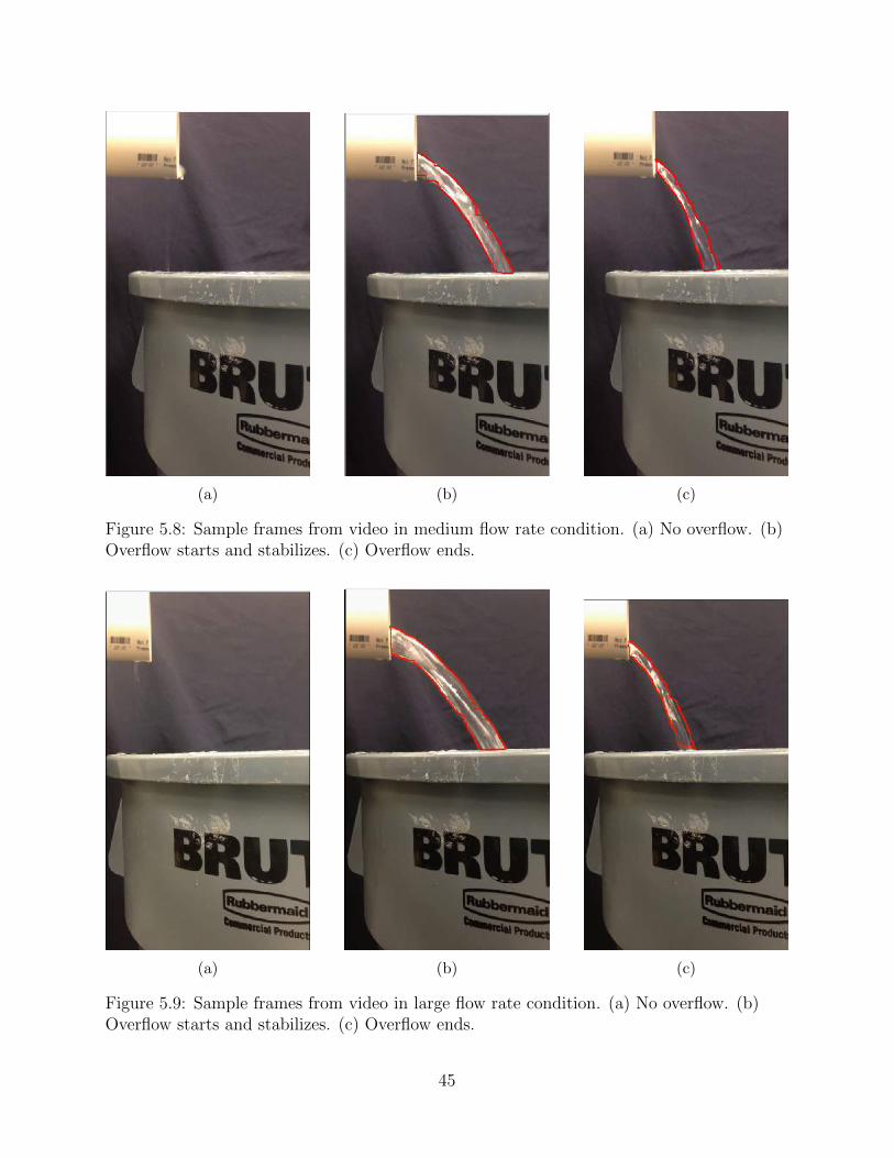
(a) (b) (c)

Figure 5.8: Sample frames from video in medium flow rate condition. (a) No overflow. (b)Overflow starts and stabilizes. (c) Overflow ends.

(a) (b) (c)

Figure 5.9: Sample frames from video in large flow rate condition. (a) No overflow. (b)Overflow starts and stabilizes. (c) Overflow ends.

45

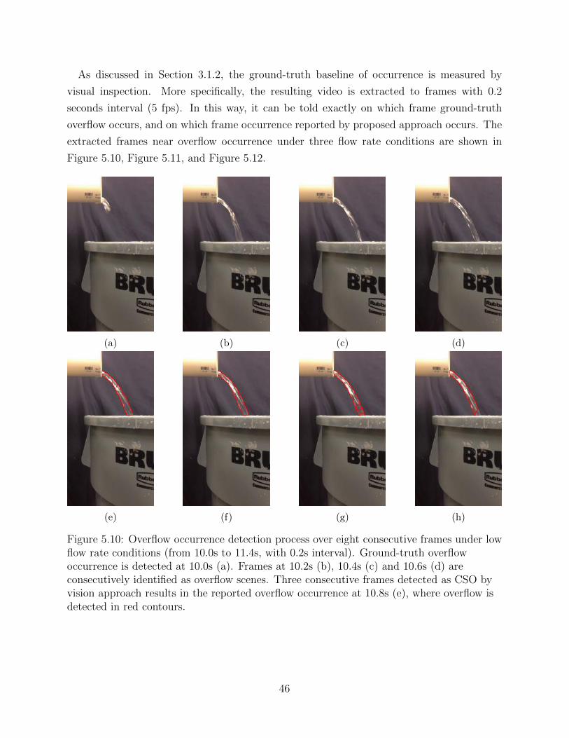
As discussed in Section 3.1.2, the ground-truth baseline of occurrence is measured by

visual inspection. More specifically, the resulting video is extracted to frames with 0.2

seconds interval (5 fps). In this way, it can be told exactly on which frame ground-truth

overflow occurs, and on which frame occurrence reported by proposed approach occurs. The

extracted frames near overflow occurrence under three flow rate conditions are shown in

Figure 5.10, Figure 5.11, and Figure 5.12.

(a) (b) (c) (d)

(e) (f) (g) (h)

Figure 5.10: Overflow occurrence detection process over eight consecutive frames under lowflow rate conditions (from 10.0s to 11.4s, with 0.2s interval). Ground-truth overflowoccurrence is detected at 10.0s (a). Frames at 10.2s (b), 10.4s (c) and 10.6s (d) areconsecutively identified as overflow scenes. Three consecutive frames detected as CSO byvision approach results in the reported overflow occurrence at 10.8s (e), where overflow isdetected in red contours.

46

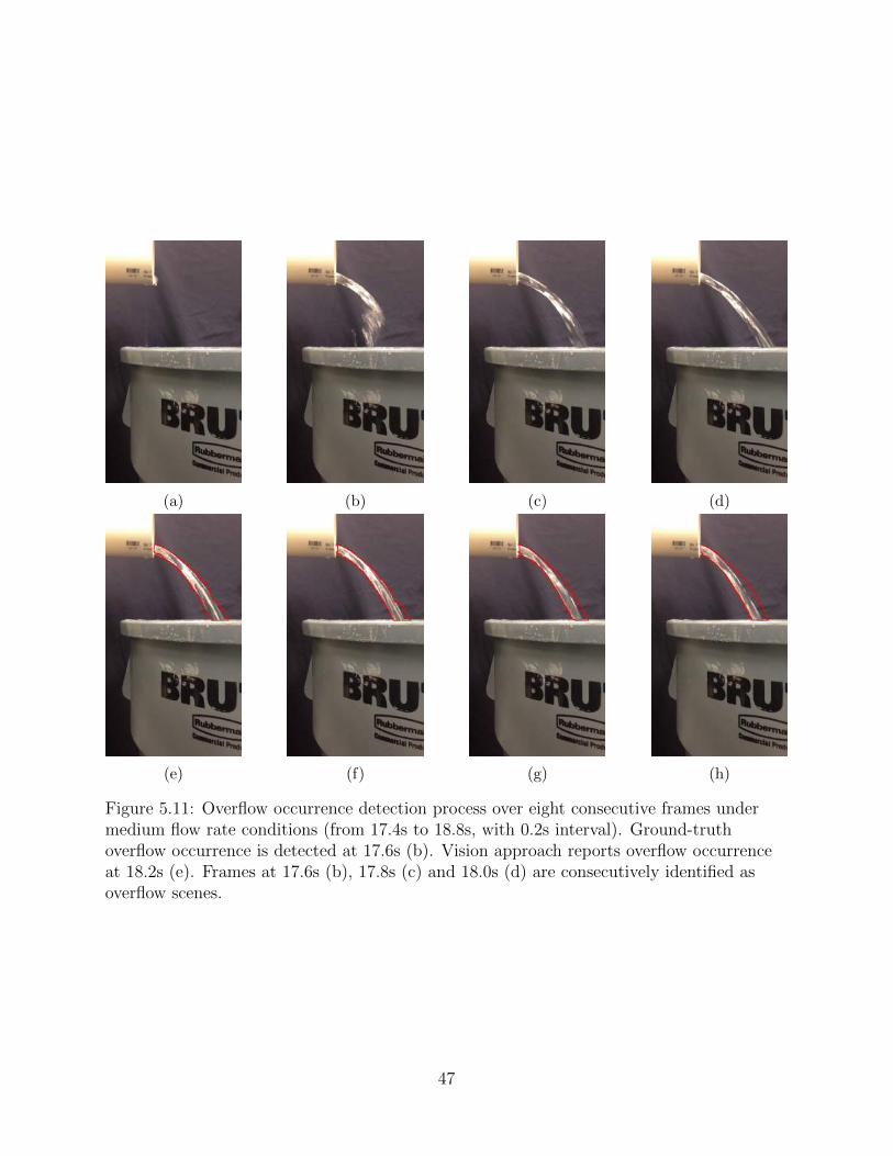
(a) (b) (c) (d)

(e) (f) (g) (h)

Figure 5.11: Overflow occurrence detection process over eight consecutive frames undermedium flow rate conditions (from 17.4s to 18.8s, with 0.2s interval). Ground-truthoverflow occurrence is detected at 17.6s (b). Vision approach reports overflow occurrenceat 18.2s (e). Frames at 17.6s (b), 17.8s (c) and 18.0s (d) are consecutively identified asoverflow scenes.

47

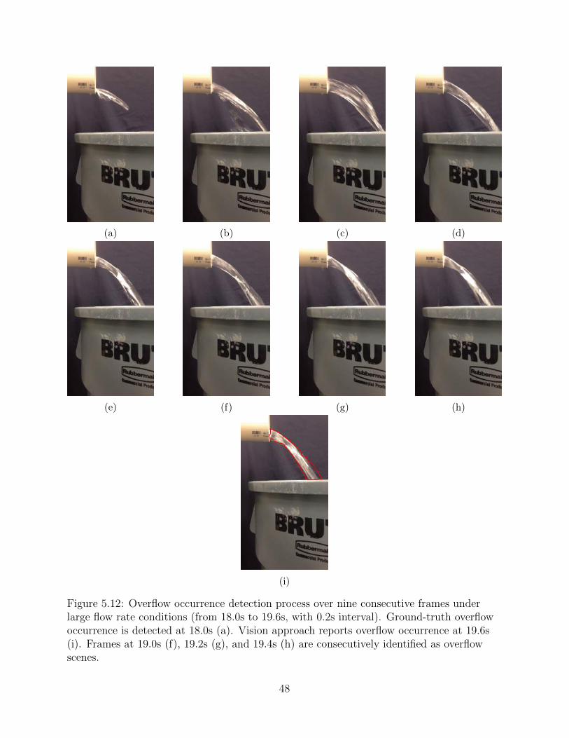
(a) (b) (c) (d)

(e) (f) (g) (h)

(i)

Figure 5.12: Overflow occurrence detection process over nine consecutive frames underlarge flow rate conditions (from 18.0s to 19.6s, with 0.2s interval). Ground-truth overflowoccurrence is detected at 18.0s (a). Vision approach reports overflow occurrence at 19.6s(i). Frames at 19.0s (f), 19.2s (g), and 19.4s (h) are consecutively identified as overflowscenes.

48

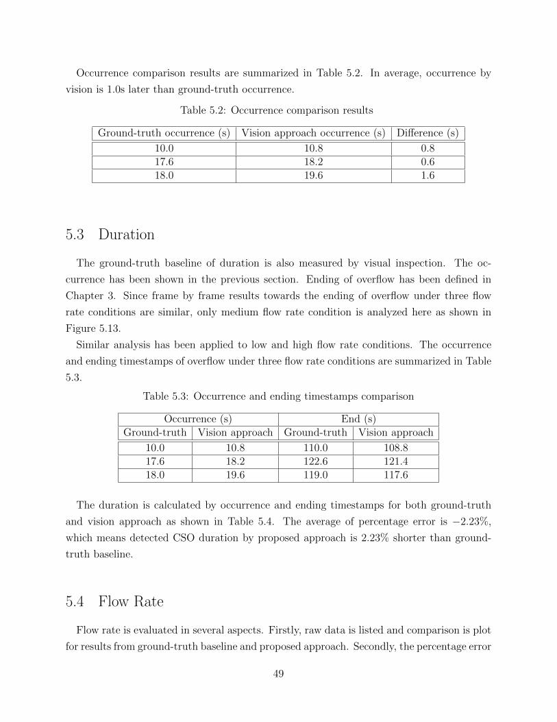
Occurrence comparison results are summarized in Table 5.2. In average, occurrence by

vision is 1.0s later than ground-truth occurrence.

Table 5.2: Occurrence comparison results

Ground-truth occurrence (s) Vision approach occurrence (s) Difference (s)

10.0 10.8 0.817.6 18.2 0.618.0 19.6 1.6

5.3 Duration

The ground-truth baseline of duration is also measured by visual inspection. The oc-

currence has been shown in the previous section. Ending of overflow has been defined in

Chapter 3. Since frame by frame results towards the ending of overflow under three flow

rate conditions are similar, only medium flow rate condition is analyzed here as shown in

Figure 5.13.

Similar analysis has been applied to low and high flow rate conditions. The occurrence

and ending timestamps of overflow under three flow rate conditions are summarized in Table

5.3.

Table 5.3: Occurrence and ending timestamps comparison

Occurrence (s) End (s)Ground-truth Vision approach Ground-truth Vision approach

10.0 10.8 110.0 108.817.6 18.2 122.6 121.418.0 19.6 119.0 117.6

The duration is calculated by occurrence and ending timestamps for both ground-truth

and vision approach as shown in Table 5.4. The average of percentage error is −2.23%,

which means detected CSO duration by proposed approach is 2.23% shorter than ground-

truth baseline.

5.4 Flow Rate

Flow rate is evaluated in several aspects. Firstly, raw data is listed and comparison is plot

for results from ground-truth baseline and proposed approach. Secondly, the percentage error

49

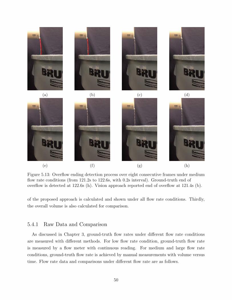
(a) (b) (c) (d)

(e) (f) (g) (h)

Figure 5.13: Overflow ending detection process over eight consecutive frames under mediumflow rate conditions (from 121.2s to 122.6s, with 0.2s interval). Ground-truth end ofoverflow is detected at 122.6s (h). Vision approach reported end of overflow at 121.4s (b).

of the proposed approach is calculated and shown under all flow rate conditions. Thirdly,

the overall volume is also calculated for comparison.

5.4.1 Raw Data and Comparison

As discussed in Chapter 3, ground-truth flow rates under different flow rate conditions

are measured with different methods. For low flow rate condition, ground-truth flow rate

is measured by a flow meter with continuous reading. For medium and large flow rate

conditions, ground-truth flow rate is achieved by manual measurements with volume versus

time. Flow rate data and comparisons under different flow rate are as follows.

50

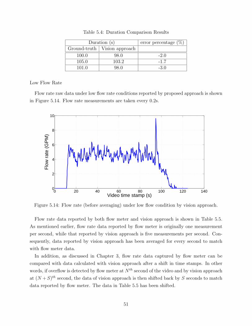
Table 5.4: Duration Comparison Results

Duration (s) error percentage (%)Ground-truth Vision approach

100.0 98.0 -2.0105.0 103.2 -1.7101.0 98.0 -3.0

Low Flow Rate

Flow rate raw data under low flow rate conditions reported by proposed approach is shown

in Figure 5.14. Flow rate measurements are taken every 0.2s.

0 20 40 60 80 100 120 1400

2

4

6

8

10

Video time stamp (s)

Flo

w r

ate

(GP

M)

Figure 5.14: Flow rate (before averaging) under low flow condition by vision approach.

Flow rate data reported by both flow meter and vision approach is shown in Table 5.5.

As mentioned earlier, flow rate data reported by flow meter is originally one measurement

per second, while that reported by vision approach is five measurements per second. Con-

sequently, data reported by vision approach has been averaged for every second to match

with flow meter data.

In addition, as discussed in Chapter 3, flow rate data captured by flow meter can be

compared with data calculated with vision approach after a shift in time stamps. In other

words, if overflow is detected by flow meter at N th second of the video and by vision approach

at (N +S)th second, the data of vision approach is then shifted back by S seconds to match

data reported by flow meter. The data in Table 5.5 has been shifted.

51

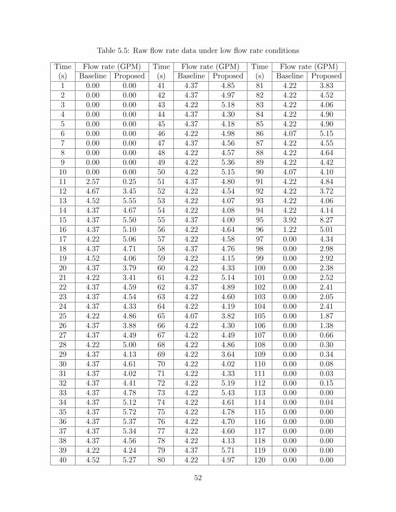
Table 5.5: Raw flow rate data under low flow rate conditions

Time Flow rate (GPM) Time Flow rate (GPM) Time Flow rate (GPM)(s) Baseline Proposed (s) Baseline Proposed (s) Baseline Proposed1 0.00 0.00 41 4.37 4.85 81 4.22 3.832 0.00 0.00 42 4.37 4.97 82 4.22 4.523 0.00 0.00 43 4.22 5.18 83 4.22 4.064 0.00 0.00 44 4.37 4.30 84 4.22 4.905 0.00 0.00 45 4.37 4.18 85 4.22 4.906 0.00 0.00 46 4.22 4.98 86 4.07 5.157 0.00 0.00 47 4.37 4.56 87 4.22 4.558 0.00 0.00 48 4.22 4.57 88 4.22 4.649 0.00 0.00 49 4.22 5.36 89 4.22 4.4210 0.00 0.00 50 4.22 5.15 90 4.07 4.1011 2.57 0.25 51 4.37 4.80 91 4.22 4.8412 4.67 3.45 52 4.22 4.54 92 4.22 3.7213 4.52 5.55 53 4.22 4.07 93 4.22 4.0614 4.37 4.67 54 4.22 4.08 94 4.22 4.1415 4.37 5.50 55 4.37 4.00 95 3.92 8.2716 4.37 5.10 56 4.22 4.64 96 1.22 5.0117 4.22 5.06 57 4.22 4.58 97 0.00 4.3418 4.37 4.71 58 4.37 4.76 98 0.00 2.9819 4.52 4.06 59 4.22 4.15 99 0.00 2.9220 4.37 3.79 60 4.22 4.33 100 0.00 2.3821 4.22 3.41 61 4.22 5.14 101 0.00 2.5222 4.37 4.59 62 4.37 4.89 102 0.00 2.4123 4.37 4.54 63 4.22 4.60 103 0.00 2.0524 4.37 4.33 64 4.22 4.19 104 0.00 2.4125 4.22 4.86 65 4.07 3.82 105 0.00 1.8726 4.37 3.88 66 4.22 4.30 106 0.00 1.3827 4.37 4.49 67 4.22 4.49 107 0.00 0.6628 4.22 5.00 68 4.22 4.86 108 0.00 0.3029 4.37 4.13 69 4.22 3.64 109 0.00 0.3430 4.37 4.61 70 4.22 4.02 110 0.00 0.0831 4.37 4.02 71 4.22 4.33 111 0.00 0.0332 4.37 4.41 72 4.22 5.19 112 0.00 0.1533 4.37 4.78 73 4.22 5.43 113 0.00 0.0034 4.37 5.12 74 4.22 4.61 114 0.00 0.0435 4.37 5.72 75 4.22 4.78 115 0.00 0.0036 4.37 5.37 76 4.22 4.70 116 0.00 0.0037 4.37 5.34 77 4.22 4.60 117 0.00 0.0038 4.37 4.56 78 4.22 4.13 118 0.00 0.0039 4.22 4.24 79 4.37 5.71 119 0.00 0.0040 4.52 5.27 80 4.22 4.97 120 0.00 0.00

52

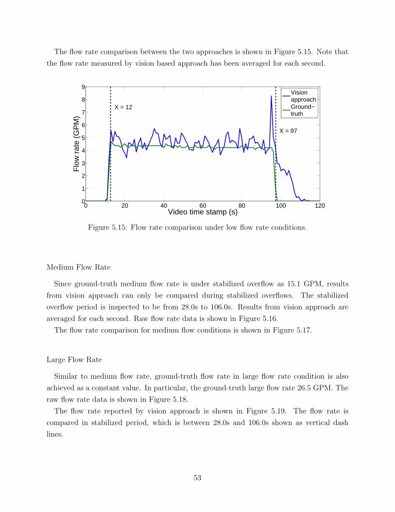
The flow rate comparison between the two approaches is shown in Figure 5.15. Note that

the flow rate measured by vision based approach has been averaged for each second.

0 20 40 60 80 100 1200

1

2

3

4

5

6

7

8

9

Video time stamp (s)

Flo

w r

ate

(GP

M)

VisionapproachGround−truth

X = 12

X = 97

Figure 5.15: Flow rate comparison under low flow rate conditions.

Medium Flow Rate

Since ground-truth medium flow rate is under stabilized overflow as 15.1 GPM, results

from vision approach can only be compared during stabilized overflows. The stabilized

overflow period is inspected to be from 28.0s to 106.0s. Results from vision approach are

averaged for each second. Raw flow rate data is shown in Figure 5.16.

The flow rate comparison for medium flow conditions is shown in Figure 5.17.

Large Flow Rate

Similar to medium flow rate, ground-truth flow rate in large flow rate condition is also

achieved as a constant value. In particular, the ground-truth large flow rate 26.5 GPM. The

raw flow rate data is shown in Figure 5.18.

The flow rate reported by vision approach is shown in Figure 5.19. The flow rate is

compared in stabilized period, which is between 28.0s and 106.0s shown as vertical dash

lines.

53

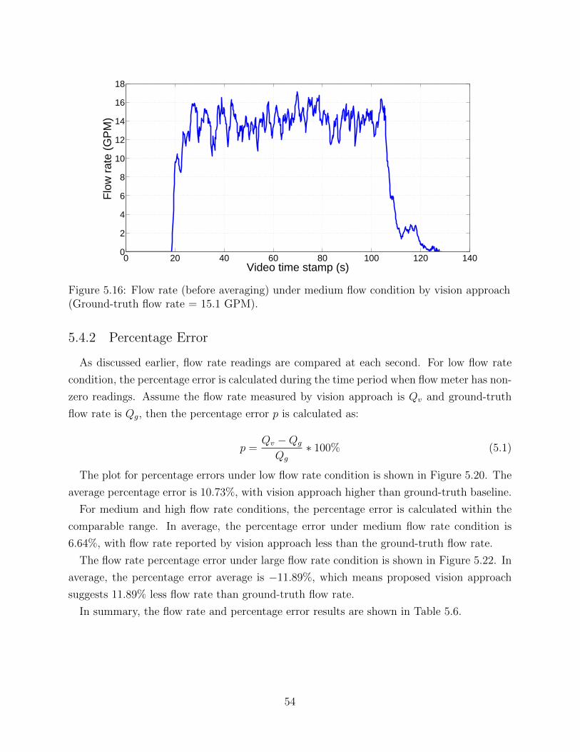
0 20 40 60 80 100 120 1400

2

4

6

8

10

12

14

16

18

Video time stamp (s)

Flo

w r

ate

(GP

M)

Figure 5.16: Flow rate (before averaging) under medium flow condition by vision approach(Ground-truth flow rate = 15.1 GPM).

5.4.2 Percentage Error

As discussed earlier, flow rate readings are compared at each second. For low flow rate

condition, the percentage error is calculated during the time period when flow meter has non-

zero readings. Assume the flow rate measured by vision approach is Qv and ground-truth

flow rate is Qg, then the percentage error p is calculated as:

p =Qv −Qg

Qg

∗ 100% (5.1)

The plot for percentage errors under low flow rate condition is shown in Figure 5.20. The

average percentage error is 10.73%, with vision approach higher than ground-truth baseline.

For medium and high flow rate conditions, the percentage error is calculated within the

comparable range. In average, the percentage error under medium flow rate condition is

6.64%, with flow rate reported by vision approach less than the ground-truth flow rate.

The flow rate percentage error under large flow rate condition is shown in Figure 5.22. In

average, the percentage error average is −11.89%, which means proposed vision approach

suggests 11.89% less flow rate than ground-truth flow rate.

In summary, the flow rate and percentage error results are shown in Table 5.6.

54

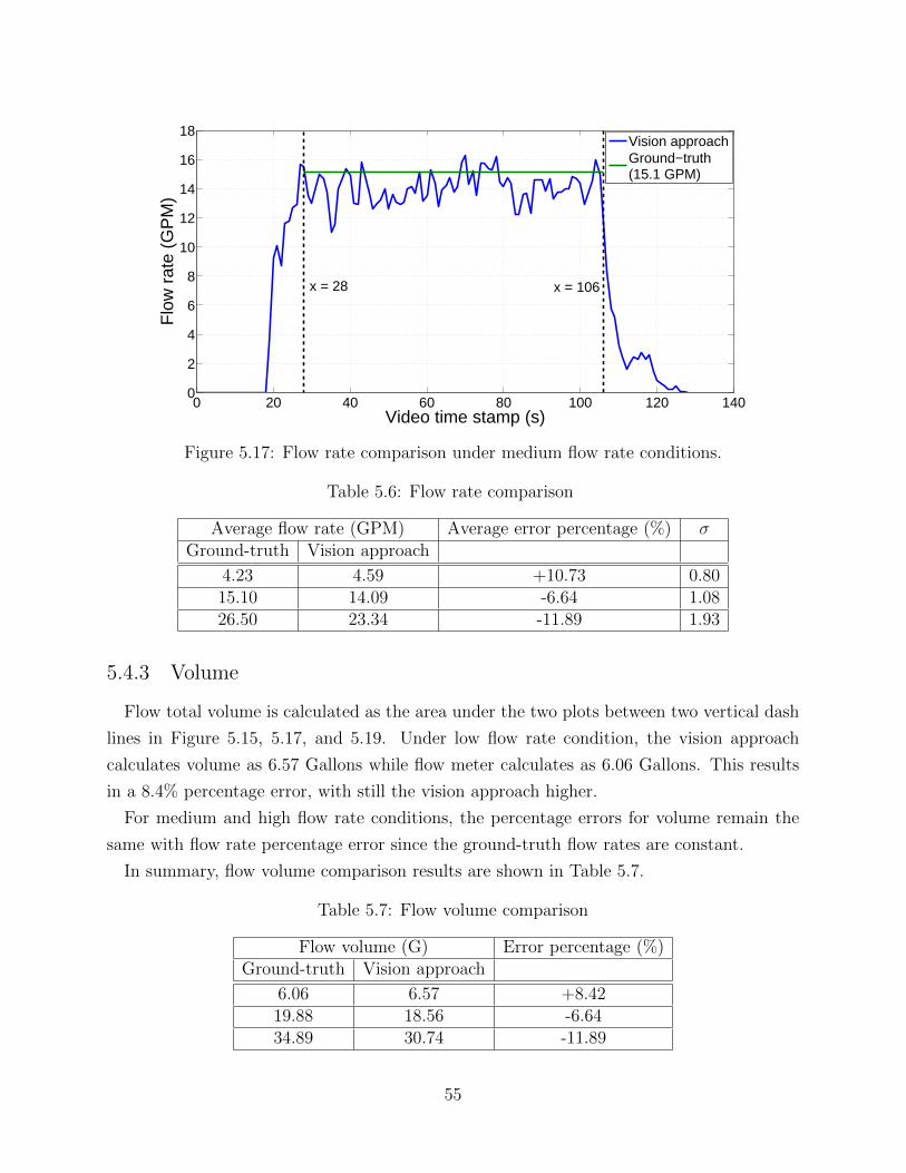
0 20 40 60 80 100 120 1400

2

4

6

8

10

12

14

16

18

Video time stamp (s)

Flo

w r

ate

(GP

M)

Vision approachGround−truth(15.1 GPM)

x = 28 x = 106

Figure 5.17: Flow rate comparison under medium flow rate conditions.

Table 5.6: Flow rate comparison

Average flow rate (GPM) Average error percentage (%) σGround-truth Vision approach

4.23 4.59 +10.73 0.8015.10 14.09 -6.64 1.0826.50 23.34 -11.89 1.93

5.4.3 Volume

Flow total volume is calculated as the area under the two plots between two vertical dash

lines in Figure 5.15, 5.17, and 5.19. Under low flow rate condition, the vision approach

calculates volume as 6.57 Gallons while flow meter calculates as 6.06 Gallons. This results

in a 8.4% percentage error, with still the vision approach higher.

For medium and high flow rate conditions, the percentage errors for volume remain the

same with flow rate percentage error since the ground-truth flow rates are constant.

In summary, flow volume comparison results are shown in Table 5.7.

Table 5.7: Flow volume comparison

Flow volume (G) Error percentage (%)Ground-truth Vision approach

6.06 6.57 +8.4219.88 18.56 -6.6434.89 30.74 -11.89

55

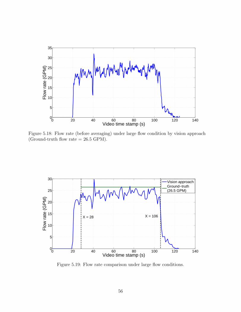
0 20 40 60 80 100 120 1400

5

10

15

20

25

30

35

Video time stamp (s)

Flo

w r

ate

(GP

M)

Figure 5.18: Flow rate (before averaging) under large flow condition by vision approach(Ground-truth flow rate = 26.5 GPM).

0 20 40 60 80 100 120 1400

5

10

15

20

25

30

Video time stamp (s)

Flo

w r

ate

(GP

M)

Vision approachGround−truth(26.5 GPM)

X = 106X = 28

Figure 5.19: Flow rate comparison under large flow conditions.

56

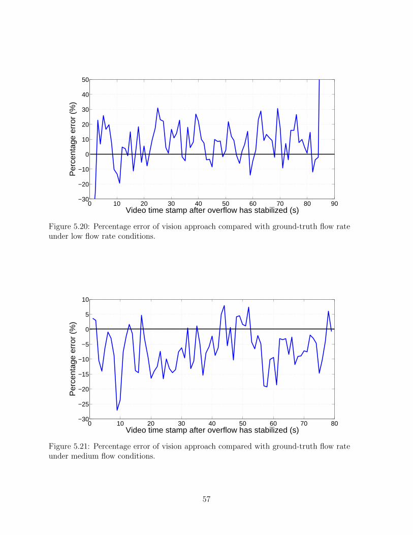
0 10 20 30 40 50 60 70 80 90−30

−20

−10

0

10

20

30

40

50

Video time stamp after overflow has stabilized (s)

Per

cent

age

erro

r (%

)

Figure 5.20: Percentage error of vision approach compared with ground-truth flow rateunder low flow rate conditions.

0 10 20 30 40 50 60 70 80−30

−25

−20

−15

−10

−5

0

5

10

Video time stamp after overflow has stabilized (s)

Per

cent

age

erro

r (%

)

Figure 5.21: Percentage error of vision approach compared with ground-truth flow rateunder medium flow conditions.

57

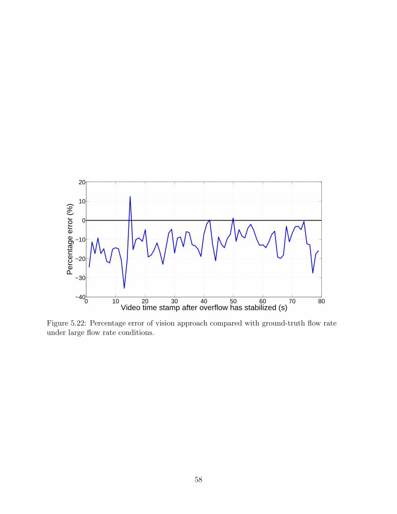
0 10 20 30 40 50 60 70 80−40

−30

−20

−10

0

10

20

Video time stamp after overflow has stabilized (s)

Per

cent

age

erro

r (%

)

Figure 5.22: Percentage error of vision approach compared with ground-truth flow rateunder large flow rate conditions.

58

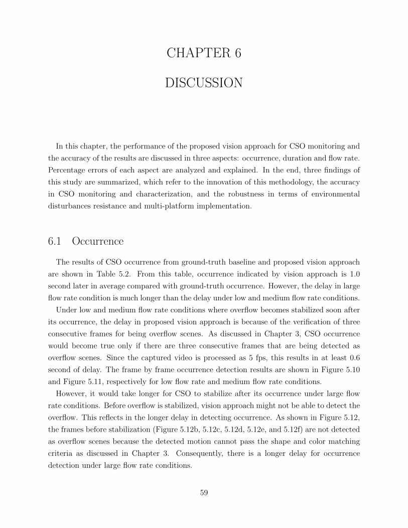
CHAPTER 6

DISCUSSION

In this chapter, the performance of the proposed vision approach for CSO monitoring and

the accuracy of the results are discussed in three aspects: occurrence, duration and flow rate.

Percentage errors of each aspect are analyzed and explained. In the end, three findings of

this study are summarized, which refer to the innovation of this methodology, the accuracy

in CSO monitoring and characterization, and the robustness in terms of environmental

disturbances resistance and multi-platform implementation.

6.1 Occurrence

The results of CSO occurrence from ground-truth baseline and proposed vision approach

are shown in Table 5.2. From this table, occurrence indicated by vision approach is 1.0

second later in average compared with ground-truth occurrence. However, the delay in large

flow rate condition is much longer than the delay under low and medium flow rate conditions.

Under low and medium flow rate conditions where overflow becomes stabilized soon after

its occurrence, the delay in proposed vision approach is because of the verification of three

consecutive frames for being overflow scenes. As discussed in Chapter 3, CSO occurrence

would become true only if there are three consecutive frames that are being detected as

overflow scenes. Since the captured video is processed as 5 fps, this results in at least 0.6

second of delay. The frame by frame occurrence detection results are shown in Figure 5.10

and Figure 5.11, respectively for low flow rate and medium flow rate conditions.

However, it would take longer for CSO to stabilize after its occurrence under large flow

rate conditions. Before overflow is stabilized, vision approach might not be able to detect the

overflow. This reflects in the longer delay in detecting occurrence. As shown in Figure 5.12,

the frames before stabilization (Figure 5.12b, 5.12c, 5.12d, 5.12e, and 5.12f) are not detected

as overflow scenes because the detected motion cannot pass the shape and color matching

criteria as discussed in Chapter 3. Consequently, there is a longer delay for occurrence

detection under large flow rate conditions.

59

In summary, the discussions above explain why vision approach reported occurrence is 1.0

second later than ground-truth occurrence in average, and why there is a longer delay for

large flow rate condition.

6.2 Duration

The duration contains two key time stamps to compare, occurrence and ending. The

timestamps for occurrence and ending of overflow are shown in Table 5.3. Occurrence has

been discussed in the previous section.

In this study, ending of an overflow event is defined as no horizontal displacement after

water flows out of pipe outlet. The definition of ending of overflow might be different under

different scenarios, e.g. it might be defined as no overflow at all. However, other scenarios

are not discussed in this thesis.

As discussed in Chapter 3, the end of overflow is determined by detecting whether there

is motion or not. Motion is detected by the percentage of foreground motion compared with

the frame size. Consequently, if the scene is detected as static, then overflow has ended.

In summary, the ending of overflow reported by proposed vision approach is 1.27 seconds

earlier than ground-truth baseline. By combining occurrence and ending, the duration is

calculated as shown in Table 5.4. In average, overflow duration reported by proposed vi-

sion approach is 2.27 seconds shorter than ground-truth baseline. The error percentage of

duration is within 3.0%.

6.3 Flow Rate

In average, proposed vision approach reports higher measurements of flow rate under low

flow rate condition compared with ground-truth baseline, while reports lower measurements

than ground-truth baseline under medium and large flow rate conditions. Since the ground-

truth pixel coordinates of detected overflow region is difficult to retrieve manually, the results

are evaluated qualitatively.

To understand the reason for performance difference under different flow rate conditions,

the frame by frame binary images of detected region are shown in Figure 6.1. White pixels

indicate the detected overflow region, while the red line shows the fitted parabola for overflow.

If we match with overflow model as shown in Figure 3.5, we can see that Point 1 and Point

3 are estimated accurately according to the parabola, while x2 of Point 2 is over estimated.

60

According to Equation 3.2, a larger x2 leads to a larger W. According to Equation 3.6, a

larger W would lead to a larger Q. This explains why proposed vision approach reports

higher flow rate than ground-truth baseline under low flow rate condition.

(a) (b) (c) (d)

(e) (f) (g) (h)

Figure 6.1: Detected binary overflow frames with fitted parabola under low flow rateconditions (from 33.4s to 34.8s, with 0.2s interval).

For medium and large flow rate conditions, flow rates reported by vision approach are lower

than ground-truth flow rates. As shown in Figure 6.2 and Figure 6.3, Point 2 and Point 3

are estimated accurately, while y1 of Point 1 is underestimated. According to Equation 3.2

and 3.4, a smaller y1 would lead to underestimated W and D. According to Equation 3.6,

the underestimated W and D both reduce Qh. This explains why proposed vision approach

reports lower flow rate than ground-truth baseline under medium and large rate conditions.

Compared with medium flow condition, the underestimation of y1 is more obvious for large

flow rate condition. This explains why larger flow rate leads to a larger error percentage.

61

(a) (b) (c) (d)

(e) (f) (g) (h)

Figure 6.2: Detected binary overflow frames with fitted parabola under medium flow ratecondition (from 37.2s to 38.6s, with 0.2s interval).

6.4 Findings

There are three main findings of this study as follows. Firstly, this study proves that

visual sensing techniques can be deployed to determine CSO occurrence, duration and flow

rate with decent accuracy by capturing the outlet points of CSS. As stated in Chapter 1, this

is the very first proposed methodology that applies computer vision techniques to monitor

CSO from outlet points. The laboratory results of this study report only 1.0s delay in

occurrence detection, and within 3.0% shorter in duration detection compared with ground-

truth baselines. As for flow rate, they are within 11.89% off by the ground-truth baselines,

and the average error percentage is 9.75%. Although these results are under laboratory

simulations, they are very promising for field deployment. Consequently, it is found that

visual sensing techniques can be deployed to determine characteristics by monitoring outlet

points.

Secondly, it is also found in this study that low cost and accurate CSO monitoring can be

achieved with minimal installation efforts as well as minimal contact. As discussed Chapter

1, this study is aimed for an easy deployment. Current practices commonly take up lots

of efforts for initial setup and data retrieval. Also cost is another issue for most of current

62

(a) (b) (c) (d)

(e) (f) (g) (h)

Figure 6.3: Detected binary overflow frames with fitted parabola under large flow ratecondition (from 37.2s to 38.6s, with interval of 0.2s).

practices that are fully capable of characterizing occurrence, duration and flow rate. This

study proposed a low-cost approach with minimal installation efforts. With only an iPhone

and its mounting devices needed, the estimated cost per CSS is under $700. For installation

efforts, the required devices are installed outside of sewer channels with easy accessibility,

instead of inside the sewer channels. Consequently, it requires minimal installation efforts

with very low cost.

Thirdly, the proposed methodology is robust enough to detect CSOs under environmental

disturbances for both real-time and forensic analysis. It is shown that the proposed method-

ology is able to identify CSOs from environmental disturbances under laboratory conditions,

e.g. moving hand and moving bottle. In addition, applications are being developed on both

iOS and Windows platforms. With the algorithm package running at back-end, iPhone 5

can achieve real-time video capturing and processing. Windows version application allows

for video processing nearly twice as fast as real-time and provides user-friendly flow rate

plots. It is feasible for forensic analysis and investigations. The resistance to environmental

disturbances and multi-platform applications make it robust and reliable for CSO monitor-

ing.

63

CHAPTER 7

CONCLUSION

7.1 Summary

Combined Sewer Overflows (CSOs) have become a major concern for water pollution prob-

lems in the United States. However, there are currently no long-term, low-cost and accurate

method to characterize CSO in terms of occurrence, duration and flow rate from an outlet

points that exists in any urban water infrastructure. Current approaches includes using in

situ sensors and prediction models. In situ sensors are usually installed inside the sewer

chambers, in which the harsh environment limits the reliability. Prediction models usually

rely on rainfall radar data and its capability to conduct real-time flow rate measurement is

very limited.

Given the constraints of current approaches, this study aimed to fill the gap by proposing

a computer vision approach for sewer overflow monitoring. Instead of installing sensors

inside sewer chambers, this methodology suggested video capture be outside of the sewer

systems and focused on outlet points. This approach was based on a model that takes

in the dimensions of the diameters of sewer outlets and the distances between the bottom

of the outlets and the water plane. Motion was first detected by background subtraction

method, and then CSO was identified based on its shape and color features. Once CSO was

detected, a parabola was fitted to help identify the initial speed and wetted area of CSO in

the pipe. This algorithm package was implemented in a Windows desktop application, as

well as an iOS application. The performance of this computer vision approach was evaluated

under laboratory environments with three flow rate conditions. In average, CSO occurrence

reported by computer vision approach is 1.0 second later than ground-truth baseline. The

percentage error of duration is 2.67% in average and within 3% under all flow rate conditions.

As for flow rate, the percentage error is within 12% under all flow conditions and 9.75% in

average.

It is found in this study that visual sensing techniques can be deployed to determine CSO

occurrence, duration and flow rate with decent accuracy by capturing the outlet points of

64

CSS. This finding is important because this is the very first study that monitors CSOs from

outlet points, and the decent results in characterization proves the feasibility of monitor-

ing CSO externally. It provides the possibility for CSO monitoring sites that are hard to be

accessed for both installation and maintenance. The computer vision approach could save ef-

forts of municipal engineers who monitor CSOs. Reliable data achieved by this methodology

are important for hydrologists who work on hydraulic models for CSOs.

In addition, it is also found that low cost CSO monitoring can be achieved with minimal

installation efforts. Prior to this study, current practices are commonly expensive and hard

to setup. The computer vision approach dramatically cuts down the cost and required

installation efforts. It is important not only for the researchers who conducted similar

studies on CSO monitoring, but also for those who work on sensing other flows, including

open channel flow, pipe flow and outflow. By realizing the feasibility and efficiency of the

computer vision approach, they could be inspired to conduct studies based on computer

vision and deploy it in smartphones.

At last, it is found that the computer vision approach is robust enough to detect CSOs

under environmental disturbances for both real-time and forensic analysis. The capability to

identify CSOs from environmental disturbances is important to applied computer scientists

who also work on identification and tracking objects by non-supervised methods. The com-

puter vision approach could also help municipal engineers who work on real-time sensing or

forensic analysis of CSOs by multi-platform support and user-friendly interfaces.

7.2 Limitations

There are two limitations of this study. The first limitation is that although occurrence

and duration achieve similar results by computer vision vision approach under all flow rate

conditions, the signals of percentage error in flow rate estimation are different. In other

words, the computer vision approach overestimates flow rate under flow rate conditions,

and underestimates flow rate under medium and large flow rate conditions. As discussed

in Chapter 6, the performance of flow rate measurement depends on how well the overflow

trajectory can be fit to a parabola. Fitted parabolas for large flow rate condition is the worst

among all flow rate conditions given the obvious offsets on starting points. To improve the

performance of the computer vision approach, flow rate may be taken into account when

modeling CSOs.

Another limitation is that the CSO model may underestimate ground-truth flow rate. In

medium flow rate condition, the parabola can be fit fairly close to the bottom contour of

65

overflow. However, it still reports a 6% less flow rate in average. The model calculates initial

velocity by the bottom trajectory, which is not exactly the average velocity of all flow layers.

In addition of uneven distribution of horizontal initial velocity, from the detected contours

in Figure 6.2, we can see that the upper bound of contour is not completely parallel with

the lower bound. In other words, its downward vertical initial velocity may also challenge

the assumptions of the model. If a downward vertical velocity is taken into consideration,

calculated horizontal initial velocity would increase. In summary, the neglect of horizontal

velocity distribution and vertical initial velocity may lead to the underestimation of flow

rate in the model.

7.3 Future Work

Future studies could be divided into several aspects. Firstly, the CSO model could be im-

proved if vertical initial velocity is taken into account. With one more unknown parameter,

it is still solvable by fitting parabola to the overflow trajectory. By adding the vertical initial

velocity in the model, the horizontal initial velocity would potentially increase. Secondly,

Manning-Strickler equation can also be integrated in CSO modeling to compensate for un-

even horizontal initial velocities of overflow. Currently, the horizontal velocity calculated by

the bottom trajectory of overflow is regarded as the horizontal velocity among all wetted

area. With Manning-Strickler equation, a more accurate model can be built for horizontal

velocity. Thirdly, the computer vision algorithm could be tested with other laboratory se-

tups, e.g. different pipe diameters, height. A sensitivity analysis could be done with respect

to the pipe sizes, height and camera angles to the scene. This would account for situations

when cameras could not be placed at the required angle. Lastly, the computer vision ap-

proach could be tested with CSO videos captured in the field. With different environment

factors and scale of flow rate, some parameters of the computer vision algorithm might need

to be tuned for better performance.

66

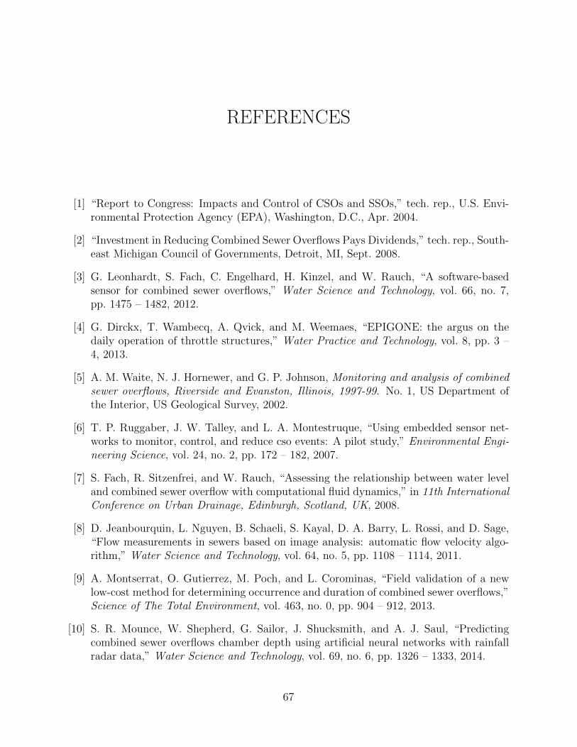
REFERENCES

[1] “Report to Congress: Impacts and Control of CSOs and SSOs,” tech. rep., U.S. Envi-ronmental Protection Agency (EPA), Washington, D.C., Apr. 2004.

[2] “Investment in Reducing Combined Sewer Overflows Pays Dividends,” tech. rep., South-east Michigan Council of Governments, Detroit, MI, Sept. 2008.

[3] G. Leonhardt, S. Fach, C. Engelhard, H. Kinzel, and W. Rauch, “A software-basedsensor for combined sewer overflows,” Water Science and Technology, vol. 66, no. 7,pp. 1475 – 1482, 2012.

[4] G. Dirckx, T. Wambecq, A. Qvick, and M. Weemaes, “EPIGONE: the argus on thedaily operation of throttle structures,” Water Practice and Technology, vol. 8, pp. 3 –4, 2013.

[5] A. M. Waite, N. J. Hornewer, and G. P. Johnson, Monitoring and analysis of combinedsewer overflows, Riverside and Evanston, Illinois, 1997-99. No. 1, US Department ofthe Interior, US Geological Survey, 2002.

[6] T. P. Ruggaber, J. W. Talley, and L. A. Montestruque, “Using embedded sensor net-works to monitor, control, and reduce cso events: A pilot study,” Environmental Engi-neering Science, vol. 24, no. 2, pp. 172 – 182, 2007.

[7] S. Fach, R. Sitzenfrei, and W. Rauch, “Assessing the relationship between water leveland combined sewer overflow with computational fluid dynamics,” in 11th InternationalConference on Urban Drainage, Edinburgh, Scotland, UK, 2008.

[8] D. Jeanbourquin, L. Nguyen, B. Schaeli, S. Kayal, D. A. Barry, L. Rossi, and D. Sage,“Flow measurements in sewers based on image analysis: automatic flow velocity algo-rithm,” Water Science and Technology, vol. 64, no. 5, pp. 1108 – 1114, 2011.

[9] A. Montserrat, O. Gutierrez, M. Poch, and L. Corominas, “Field validation of a newlow-cost method for determining occurrence and duration of combined sewer overflows,”Science of The Total Environment, vol. 463, no. 0, pp. 904 – 912, 2013.

[10] S. R. Mounce, W. Shepherd, G. Sailor, J. Shucksmith, and A. J. Saul, “Predictingcombined sewer overflows chamber depth using artificial neural networks with rainfallradar data,” Water Science and Technology, vol. 69, no. 6, pp. 1326 – 1333, 2014.

67

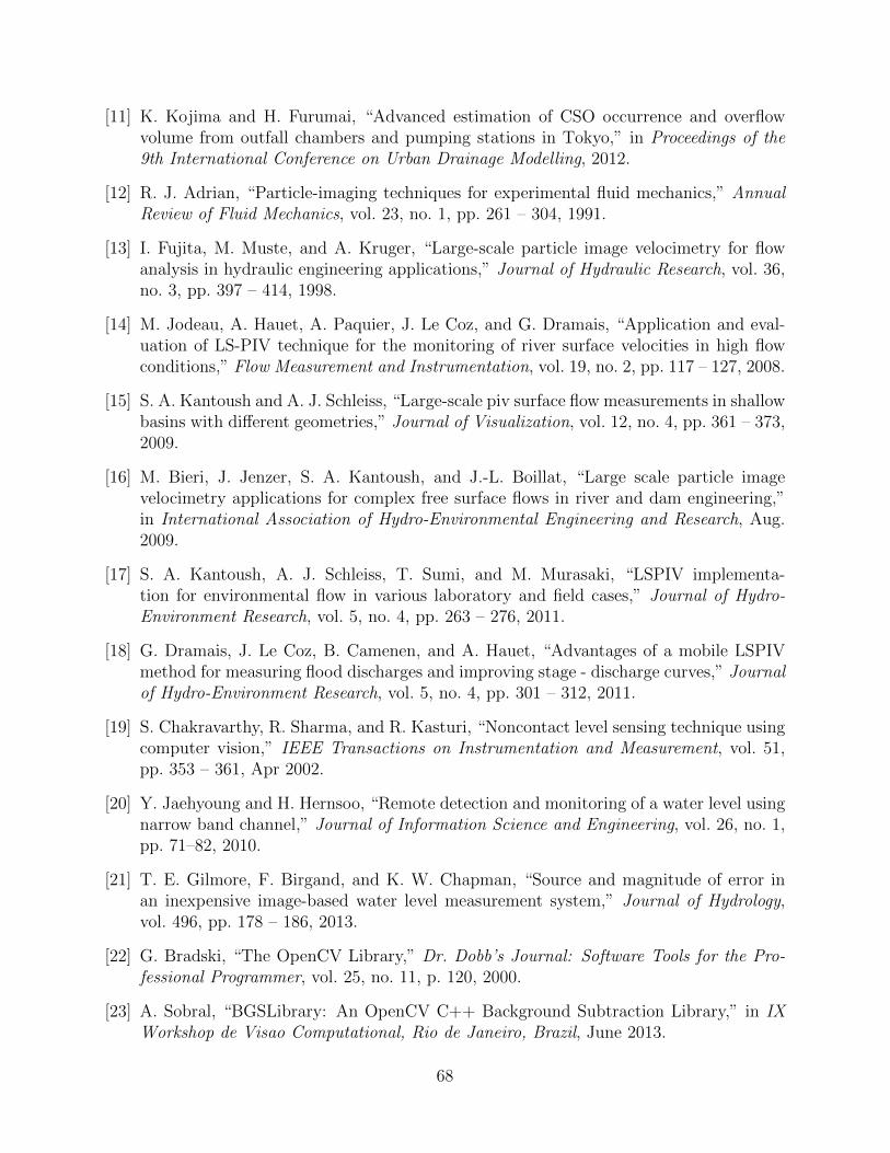
[11] K. Kojima and H. Furumai, “Advanced estimation of CSO occurrence and overflowvolume from outfall chambers and pumping stations in Tokyo,” in Proceedings of the9th International Conference on Urban Drainage Modelling, 2012.

[12] R. J. Adrian, “Particle-imaging techniques for experimental fluid mechanics,” AnnualReview of Fluid Mechanics, vol. 23, no. 1, pp. 261 – 304, 1991.

[13] I. Fujita, M. Muste, and A. Kruger, “Large-scale particle image velocimetry for flowanalysis in hydraulic engineering applications,” Journal of Hydraulic Research, vol. 36,no. 3, pp. 397 – 414, 1998.

[14] M. Jodeau, A. Hauet, A. Paquier, J. Le Coz, and G. Dramais, “Application and eval-uation of LS-PIV technique for the monitoring of river surface velocities in high flowconditions,” Flow Measurement and Instrumentation, vol. 19, no. 2, pp. 117 – 127, 2008.

[15] S. A. Kantoush and A. J. Schleiss, “Large-scale piv surface flow measurements in shallowbasins with different geometries,” Journal of Visualization, vol. 12, no. 4, pp. 361 – 373,2009.

[16] M. Bieri, J. Jenzer, S. A. Kantoush, and J.-L. Boillat, “Large scale particle imagevelocimetry applications for complex free surface flows in river and dam engineering,”in International Association of Hydro-Environmental Engineering and Research, Aug.2009.

[17] S. A. Kantoush, A. J. Schleiss, T. Sumi, and M. Murasaki, “LSPIV implementa-tion for environmental flow in various laboratory and field cases,” Journal of Hydro-Environment Research, vol. 5, no. 4, pp. 263 – 276, 2011.

[18] G. Dramais, J. Le Coz, B. Camenen, and A. Hauet, “Advantages of a mobile LSPIVmethod for measuring flood discharges and improving stage - discharge curves,” Journalof Hydro-Environment Research, vol. 5, no. 4, pp. 301 – 312, 2011.

[19] S. Chakravarthy, R. Sharma, and R. Kasturi, “Noncontact level sensing technique usingcomputer vision,” IEEE Transactions on Instrumentation and Measurement, vol. 51,pp. 353 – 361, Apr 2002.

[20] Y. Jaehyoung and H. Hernsoo, “Remote detection and monitoring of a water level usingnarrow band channel,” Journal of Information Science and Engineering, vol. 26, no. 1,pp. 71–82, 2010.

[21] T. E. Gilmore, F. Birgand, and K. W. Chapman, “Source and magnitude of error inan inexpensive image-based water level measurement system,” Journal of Hydrology,vol. 496, pp. 178 – 186, 2013.

[22] G. Bradski, “The OpenCV Library,” Dr. Dobb’s Journal: Software Tools for the Pro-fessional Programmer, vol. 25, no. 11, p. 120, 2000.

[23] A. Sobral, “BGSLibrary: An OpenCV C++ Background Subtraction Library,” in IXWorkshop de Visao Computational, Rio de Janeiro, Brazil, June 2013.

68

[24] P. KaewTraKulPong and R. Bowden, “An Improved Adaptive Background MixtureModel for Real-time Tracking with Shadow Detection,” in Video-Based SurveillanceSystems, pp. 135 – 144, Springer US, 2002.

[25] Z. Zivkovic, “Improved adaptive Gaussian mixture model for background subtraction,”in Proceedings of the 17th International Conference on Pattern Recognition, vol. 2,pp. 28 – 31, Aug 2004.

[26] M. Hofmann, P. Tiefenbacher, and G. Rigoll, “Background segmentation with feed-back: The Pixel-Based Adaptive Segmenter,” in IEEE Computer Society Conferenceon Computer Vision and Pattern Recognition Workshops, pp. 38 – 43, June 2012.

[27] J. Yao and J. Odobez, “Multi-Layer Background Subtraction Based on Color and Tex-ture,” in IEEE Conference on Computer Vision and Pattern Recognition, pp. 1 – 8,June 2007.

[28] M.-K. Hu, “Visual pattern recognition by moment invariants,” IRE Transactions onInformation Theory, vol. 8, no. 2, pp. 179 – 187, 1962.

[29] “Desktop Operating System Market Share.” http://www.netmarketshare.com/. Ac-cessed: 2014-10-20.

69

APPENDIX A WINDOWS APPLICATION USAGEINSTRUCTIONS

A.1 Background

The purpose of this document is to provide usage instructions for Overflow 1.0 (Windows

desktop version). This Overflow application is a monitoring tool to be used for forensic

analysis and investigation of CSO events. It allows a user to select a video clip of an

overflow event and visualize the resulting flow rates when it starts running. The application

creates a csv file that records flow rate at a time interval of 0.2s.

A.2 System Requirements

This application is running on 64-bit Windows systems, including Windows 7, 8, and 8.1.

A minimum of 3rd generation Intel Core i3 processor and 4GB memory is recommended.

A.3 User Interface

The design of Overflow user interface is aimed for simplicity and ease of usage. Figure

A.1 shows the main window when Overflow is opened and the labels for main components.

The main window of Overflow mainly consists of three parts: control buttons (Open...,

Run and Stop buttons), information display and interaction (video name, dimensions and

progress bar), and plotting widget. Control buttons of opening video, start and stop video

processing are displayed on upper-left. Selected video name is displayed on upper-right table.

Users specify the dimensions of pipe diameter and height. Progress bar indicates the current

progress of video processing. Flow rate versus time is plot in real-time in plotting widget.

70

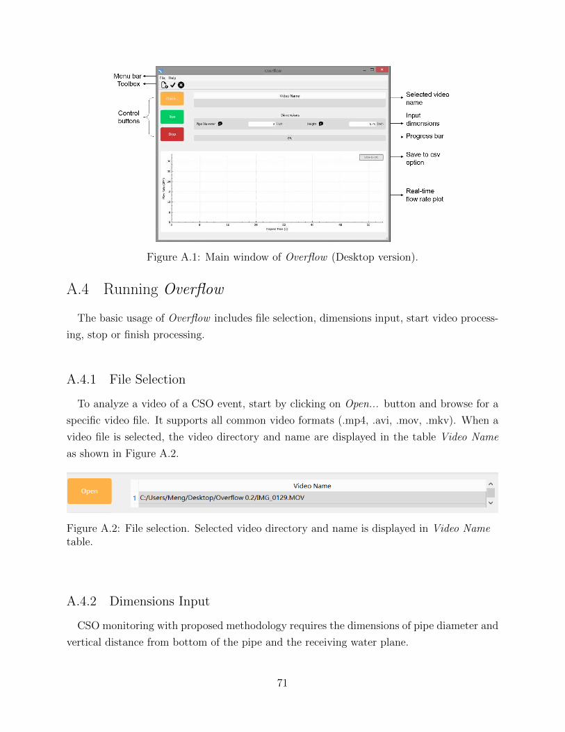
Figure A.1: Main window of Overflow (Desktop version).

A.4 Running Overflow

The basic usage of Overflow includes file selection, dimensions input, start video process-

ing, stop or finish processing.

A.4.1 File Selection

To analyze a video of a CSO event, start by clicking on Open... button and browse for a

specific video file. It supports all common video formats (.mp4, .avi, .mov, .mkv). When a

video file is selected, the video directory and name are displayed in the table Video Name

as shown in Figure A.2.

Figure A.2: File selection. Selected video directory and name is displayed in Video Nametable.

A.4.2 Dimensions Input

CSO monitoring with proposed methodology requires the dimensions of pipe diameter and

vertical distance from bottom of the pipe and the receiving water plane.

71

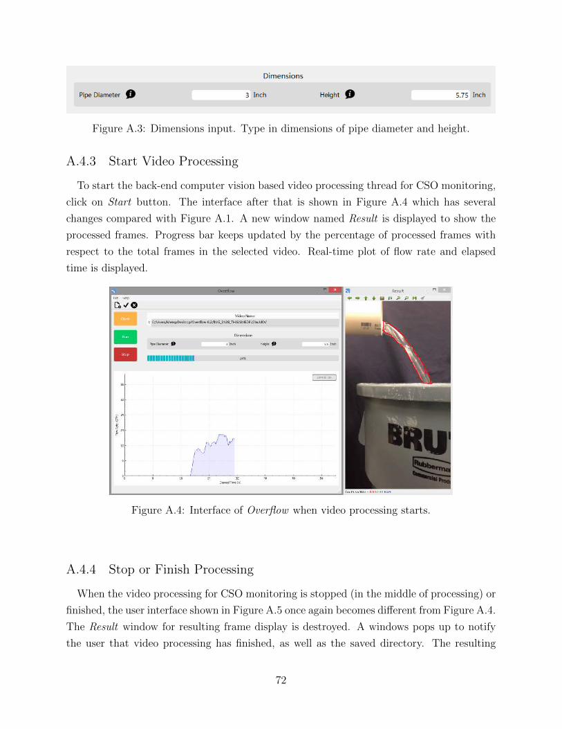
Figure A.3: Dimensions input. Type in dimensions of pipe diameter and height.

A.4.3 Start Video Processing

To start the back-end computer vision based video processing thread for CSO monitoring,

click on Start button. The interface after that is shown in Figure A.4 which has several

changes compared with Figure A.1. A new window named Result is displayed to show the

processed frames. Progress bar keeps updated by the percentage of processed frames with

respect to the total frames in the selected video. Real-time plot of flow rate and elapsed

time is displayed.

Figure A.4: Interface of Overflow when video processing starts.

A.4.4 Stop or Finish Processing

When the video processing for CSO monitoring is stopped (in the middle of processing) or

finished, the user interface shown in Figure A.5 once again becomes different from Figure A.4.

The Result window for resulting frame display is destroyed. A windows pops up to notify

the user that video processing has finished, as well as the saved directory. The resulting

72

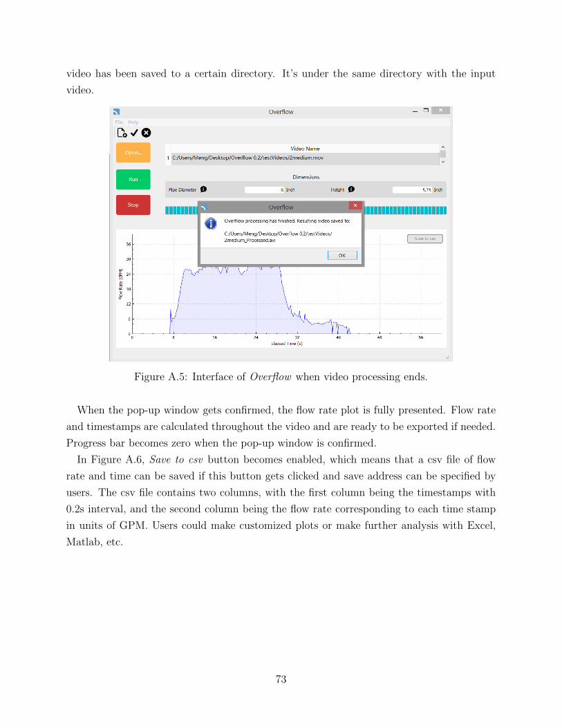
video has been saved to a certain directory. It’s under the same directory with the input

video.

Figure A.5: Interface of Overflow when video processing ends.

When the pop-up window gets confirmed, the flow rate plot is fully presented. Flow rate

and timestamps are calculated throughout the video and are ready to be exported if needed.

Progress bar becomes zero when the pop-up window is confirmed.

In Figure A.6, Save to csv button becomes enabled, which means that a csv file of flow

rate and time can be saved if this button gets clicked and save address can be specified by

users. The csv file contains two columns, with the first column being the timestamps with

0.2s interval, and the second column being the flow rate corresponding to each time stamp

in units of GPM. Users could make customized plots or make further analysis with Excel,

Matlab, etc.

73

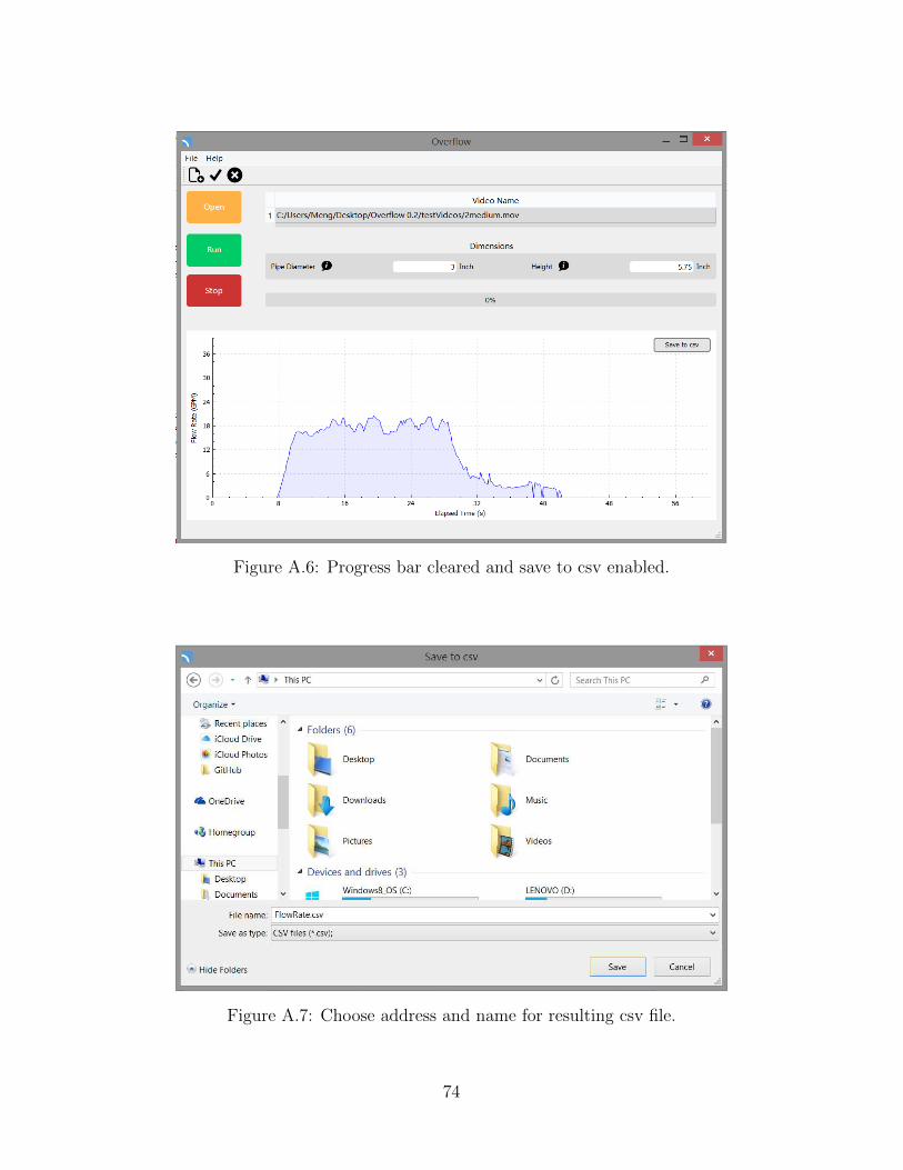
Figure A.6: Progress bar cleared and save to csv enabled.

Figure A.7: Choose address and name for resulting csv file.

74

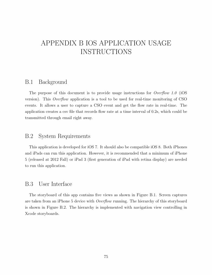
APPENDIX B IOS APPLICATION USAGEINSTRUCTIONS

B.1 Background

The purpose of this document is to provide usage instructions for Overflow 1.0 (iOS

version). This Overflow application is a tool to be used for real-time monitoring of CSO

events. It allows a user to capture a CSO event and get the flow rate in real-time. The

application creates a csv file that records flow rate at a time interval of 0.2s, which could be

transmitted through email right away.

B.2 System Requirements

This application is developed for iOS 7. It should also be compatible iOS 8. Both iPhones

and iPads can run this application. However, it is recommended that a minimum of iPhone

5 (released at 2012 Fall) or iPad 3 (first generation of iPad with retina display) are needed

to run this application.

B.3 User Interface

The storyboard of this app contains five views as shown in Figure B.1. Screen captures

are taken from an iPhone 5 device with Overflow running. The hierarchy of this storyboard

is shown in Figure B.2. The hierarchy is implemented with navigation view controlling in

Xcode storyboards.

75

(a) View 1 (b) View 2 (c) View 3

(d) View 4 (e) View 5

Figure B.1: Overflow storyboard (iOS version). (a) View 1: Homepage. Request userinput of dimensions of R and H. (b) View 2: About. Display overview and developmentteam of Overflow. (c) View 3: Video Processing. Video capture, processing and controlsare included. (d) View 4: Display results and options to save and send the result. (e) View5: Send file of flow rate through Email.

76

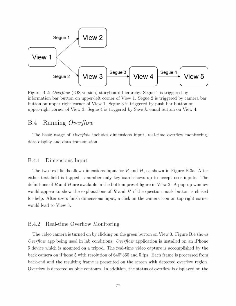
Figure B.2: Overflow (iOS version) storyboard hierarchy. Segue 1 is triggered byinformation bar button on upper-left corner of View 1. Segue 2 is triggered by camera barbutton on upper-right corner of View 1. Segue 3 is triggered by push bar button onupper-right corner of View 3. Segue 4 is triggered by Save & email button on View 4.

B.4 Running Overflow

The basic usage of Overflow includes dimensions input, real-time overflow monitoring,

data display and data transmission.

B.4.1 Dimensions Input

The two text fields allow dimensions input for R and H, as shown in Figure B.3a. After

either text field is tapped, a number only keyboard shows up to accept user inputs. The

definitions of R and H are available in the bottom preset figure in View 2. A pop-up window

would appear to show the explanations of R and H if the question mark button is clicked

for help. After users finish dimensions input, a click on the camera icon on top right corner

would lead to View 3.

B.4.2 Real-time Overflow Monitoring

The video camera is turned on by clicking on the green button on View 3. Figure B.4 shows

Overflow app being used in lab conditions. Overflow application is installed on an iPhone

5 device which is mounted on a tripod. The real-time video capture is accomplished by the

back camera on iPhone 5 with resolution of 640*360 and 5 fps. Each frame is processed from

back-end and the resulting frame is presented on the screen with detected overflow region.

Overflow is detected as blue contours. In addition, the status of overflow is displayed on the

77

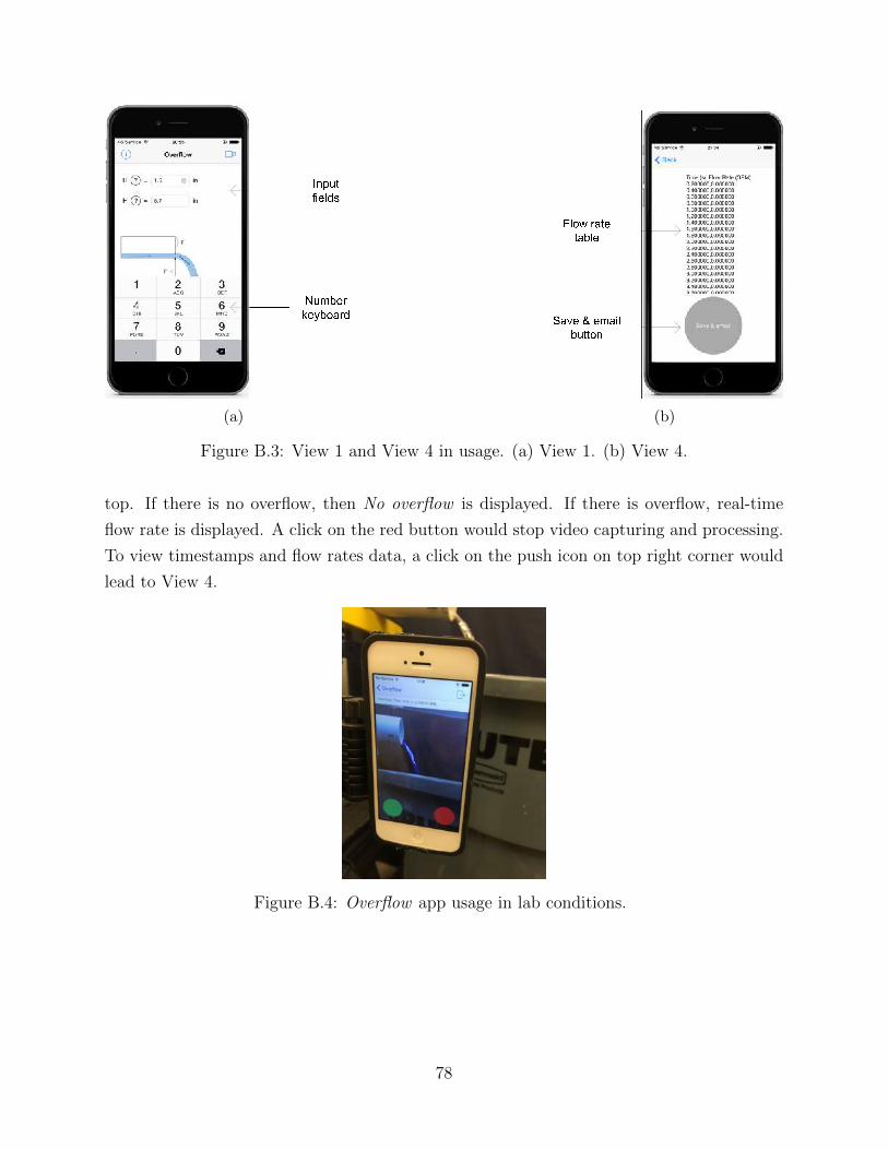
(a) (b)

Figure B.3: View 1 and View 4 in usage. (a) View 1. (b) View 4.

top. If there is no overflow, then No overflow is displayed. If there is overflow, real-time

flow rate is displayed. A click on the red button would stop video capturing and processing.

To view timestamps and flow rates data, a click on the push icon on top right corner would

lead to View 4.

Figure B.4: Overflow app usage in lab conditions.

78

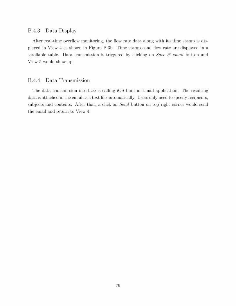
B.4.3 Data Display

After real-time overflow monitoring, the flow rate data along with its time stamp is dis-

played in View 4 as shown in Figure B.3b. Time stamps and flow rate are displayed in a

scrollable table. Data transmission is triggered by clicking on Save & email button and

View 5 would show up.

B.4.4 Data Transmission

The data transmission interface is calling iOS built-in Email application. The resulting

data is attached in the email as a text file automatically. Users only need to specify recipients,

subjects and contents. After that, a click on Send button on top right corner would send

the email and return to View 4.

79