A Computational Auditory Scene Analysis-Enhanced Beamforming Approach for Sound Source Separation

Hindawi Publishing CorporationEURASIP Journal on Advances in Signal ProcessingVolume 2009, Article ID 403681, 17 pagesdoi:10.1155/2009/403681

Research Article

A Computational Auditory Scene Analysis-EnhancedBeamforming Approach for Sound Source Separation

L. A. Drake,1 J. C. Rutledge,2 J. Zhang,3 and A. Katsaggelos (EURASIP Member)4

1 JunTech Inc., 2314 E. Stratford Ct, Shorewood, WI 53211, USA2 Computer Science and Electrical Engineering Department, University of Maryland, Baltimore County, Baltimore, MD 21250, USA3 Electrical Engineering and Computer Science Department, University of Wisconsin-Milwaukee, Milwaukee, WI 53201, USA4 Department of Electrical Engineering and Computer Science, Northwestern University, Evanston, IL 60208, USA

Correspondence should be addressed to L. A. Drake, [email protected]

Received 1 December 2008; Revised 18 May 2009; Accepted 12 August 2009

Recommended by Henning Puder

Hearing aid users have difficulty hearing target signals, such as speech, in the presence of competing signals or noise. Most solutionsproposed to date enhance or extract target signals from background noise and interference based on either location attributes orsource attributes. Location attributes typically involve arrival angles at a microphone array. Source attributes include characteristicsthat are specific to a signal, such as fundamental frequency, or statistical properties that differentiate signals. This paper describes anovel approach to sound source separation, called computational auditory scene analysis-enhanced beamforming (CASA-EB), thatachieves increased separation performance by combining the complementary techniques of CASA (a source attribute technique)with beamforming (a location attribute technique), complementary in the sense that they use independent attributes for signalseparation. CASA-EB performs sound source separation by temporally and spatially filtering a multichannel input signal, and thengrouping the resulting signal components into separated signals, based on source and location attributes. Experimental resultsshow increased signal-to-interference ratio with CASA-EB over beamforming or CASA alone.

Copyright © 2009 L. A. Drake et al. This is an open access article distributed under the Creative Commons Attribution License,which permits unrestricted use, distribution, and reproduction in any medium, provided the original work is properly cited.

1. Introduction

People often find themselves in cluttered acoustic envi-ronments, where what they want to listen to is mixedwith noise, interference, and other acoustic signals of nointerest. The problem of extracting an acoustic signal ofinterest from background clutter is called sound sourceseparation and, in psychoacoustics, is also known as the“cocktail party problem.” Such “hearing out” of a desiredsignal can be particularly challenging for hearing aid userswho often have reduced localization abilities. Sound sourceseparation could allow them to distinguish better betweenmultiple speakers, and thus, hear a chosen speaker moreclearly. Separated signals from a sound source separationsystem can be further enhanced through techniques suchas amplitude compression for listeners with sensorineuralhearing loss and are also suitable for further processingin other applications, such as teleconferencing, automaticspeech recognition, automatic transcription of ensemblemusic, and modeling the human auditory system.

There are three main approaches to the general soundsource separation problem: blind source separation methods,those that use location attributes, and those that use sourceattributes. Blind source separation techniques separatesound signals based on the assumption that the signals are“independent,” that is, that their nth-order joint momentsare equal to zero. When 2nd-order statistics are used, themethod is called principal component analysis (PCA); whenhigher-order statistics are used, it is called independentcomponent analysis (ICA). Blind source separation methodscan achieve good performance. However, they require theobservation data to satisfy some strict assumptions that maynot be compatible with a natural listening environment.Besides the “independence” requirement, they can alsorequire one or more of the following: a constant mixingprocess, a known and fixed number of sources, and anequal number of sources and observations [1]. Locationand source attribute-based methods do not require any ofthese, and thus, are effective for a wider range of listeningenvironments.

2 EURASIP Journal on Advances in Signal Processing

Location attributes describe the physical location ofa sound source at the time it produced the sound. Forexample, a sound passes across a microphone array fromsome direction, and this direction, called “arrival angle,” isa location attribute. One location-attribute-based techniqueis binaural CASA [2–4]. Based on a model of the humanauditory system, binaural sound source separation usesbinaural data (sound “heard” at two “ears”) to estimatethe arrival angle of “dominant” single-source sounds. Itdoes this by comparing the binaural data’s interaural timedelays and interaural intensity differences to a look-uptable and selecting the closest match. While binaural CASAperformance is impressive for a two microphone array (twoears), improved performance may be achieved by usinglarger arrays—as in beamforming. In addition to lifting thetwo microphone restriction of binaural CASA, microphonearray processing is also more amenable to quantitativeperformance analysis since it is a mathematically derivedapproach.

Beamforming uses spatially sampled data from an arrayof two or more sensors to estimate arrival angles andwaveforms of “dominant” signals in the wavefield. Generally,the idea is to combine the sensor measurements in someway so that desirable signals add constructively, while noiseand interference are reduced. Various beamforming methods(taken and adapted from traditional array processing forapplications such as radar and sonar) have been developedfor and applied to speech and other acoustic signals. A reviewof these “microphone array processing” methods can befound in [5]. Regardless of which specific location methodis chosen, however, and how well it works, it still cannotseparate signals from the same (or from a close) locationsince location is its cue for separation [6].

In this paper, we present a novel technique combiningbeamforming with a source attribute technique, monauralCASA. This category of source attribute methods modelshow human hearing separates multispeaker input to “hearout” each speaker individually. Source attributes describethe state of the sound source at the time it producesthe sound. For example, in the case of a voiced speechsound, fundamental frequency (F0) is a source attribute thatindicates the rate at which the speaker’s glottis opens andcloses. Monaural CASA [3, 7–12] is based on a model ofhow the human auditory system performs monaural soundsource separation. It groups “time-frequency” signal com-ponents with similar source attributes, such as fundamentalfrequency (F0), amplitude modulation (AM), onset/offsettimes and timbre. Such signal component groups then givethe separated sounds.

Location-attribute techniques can separate signals betterin some situations than source-attribute techniques can.For example, since location attributes are independent ofsignal spectral characteristics, they can group harmonic andinharmonic signals equally well. Source-attribute techniquessuch as monaural CASA, on the other hand, have troublewith inharmonic signals. Similarly, when a signal changes itsspectral characteristics abruptly, for example, from a fricativeto a vowel in a speech signal, the performance of location-attribute techniques will not be affected. Source-attribute

techniques, on the other hand, may mistakenly separate thefricative and the vowel—assigning them to different soundsources.

Source-attribute techniques can also perform better thanlocation-attribute methods in some situations. Specifically,they can separate sound mixtures in which the single-sourcesignals have close or equal arrival angles. Their complemen-tary strengths suggest that combining these two techniquesmay provide better sound source separation performancethan using either method individually. Indeed, previouslypublished work combining monaural and binaural CASAshows that this is a promising idea ([3, 13]).

In this paper, we exploit the idea of combining locationand source attributes further by combining beamformingwith monaural CASA into a novel approach called CASA-Enhanced Beamforming (CASA-EB). The main reason forusing beamforming rather than binaural CASA as thelocation-attribute technique, here, is that beamformingmay provide higher arrival angle resolution through theuse of larger microphone arrays and adaptive processing.In addition, beamforming is more subject to quantitativeanalysis.

2. CASA-EB Overview

We begin by introducing some notation and giving a moreprecise definition of sound source separation. Suppose amultisource sound field is observed by an array ofM acousticsensors (microphones). This produces M observed mixturesignals:

y[m,n] =K∑

k=1

xk[m,n] +w[m,n], m = 1, 2, . . . ,M, (1)

where n is the time index, m is the microphone index,xk[m,n] is the kth source signal as observed at the mthmicrophone, and w[m,n] is the noise in the observation(background and measurement noise). The goal of soundsource separation, then, is to make an estimate of each of theK single-source signals in the observed mixture signals

x̂k[n], k ∈ {1, 2, . . . ,K}, (2)

where ∧ is used to indicate estimation, and the estimate x̂k[n]may differ from the source signal by a delay and/or scalefactor.

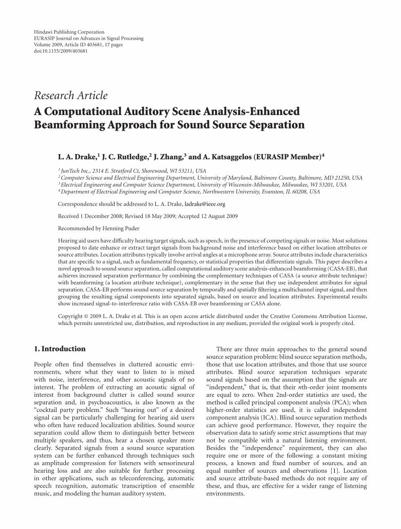
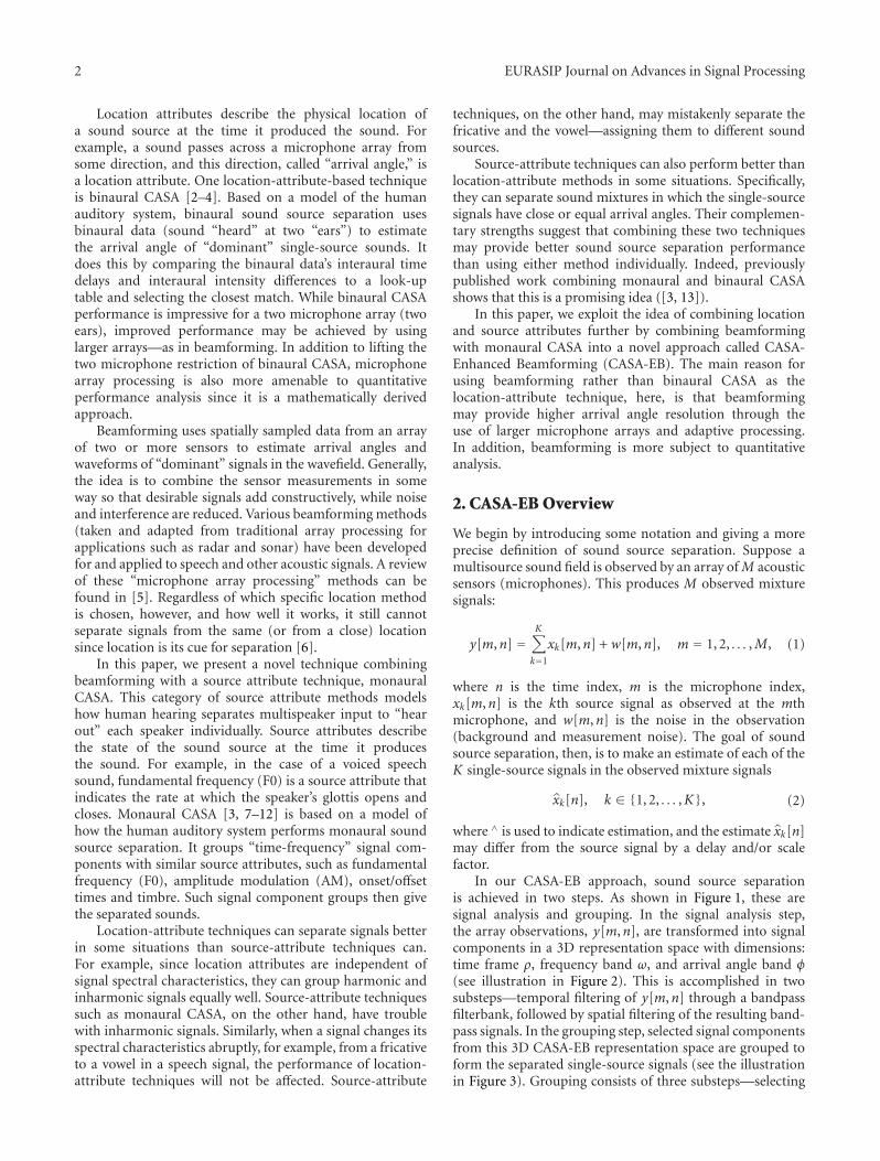
In our CASA-EB approach, sound source separationis achieved in two steps. As shown in Figure 1, these aresignal analysis and grouping. In the signal analysis step,the array observations, y[m,n], are transformed into signalcomponents in a 3D representation space with dimensions:time frame ρ, frequency band ω, and arrival angle band φ(see illustration in Figure 2). This is accomplished in twosubsteps—temporal filtering of y[m,n] through a bandpassfilterbank, followed by spatial filtering of the resulting band-pass signals. In the grouping step, selected signal componentsfrom this 3D CASA-EB representation space are grouped toform the separated single-source signals (see the illustrationin Figure 3). Grouping consists of three substeps—selecting

EURASIP Journal on Advances in Signal Processing 3

Signal analysis

Spat

ial

filt

erin

g

Tem

por

alfi

lter

ing

Arr

ival

angl

e(φ

)de

tect

ion

Freq

uen

cyba

nd

(ω)

sele

ctio

n

Signal componentselection

Sourceattribute

(F0)

Locationattribute

(φ)

Shor

t-ti

me

sequ

enti

al

Sim

ult

aneo

us

Lin

kin

gsh

ort-

tim

egr

oups

Signal componentgrouping

Wav

efor

mre

syn

thes

is

Attributeestimation

Grouping

Figure 1: Block diagram of CASA-EB.

The CASA-EBrepresentation

of a siren.

The projection in thetime-frequency plane is

a spectrogram of the siren.

The projection in thetime-arrival angle plane shows

the siren’s arrival angle, φ0.

ρ

φ

φ0

ω

(a)

The CASA-EBrepresentation

of harmonic signal.

The projection in thetime-frequency plane is a spectrogram

of the harmonic signal.

The projection in thetime-arrival angle plane shows

the signal’s arrival angle, φ0.

ρ

φ

φ0

ω

(b)

Figure 2: CASA-EB representations of a siren (a), and a simpleharmonic signal (b). The projections on the time-frequency plane(signal’s spectrogram) and time-arrival angle planes (signal’s arrivalangle path) are also shown.

signal components to group, estimating their attributes,and finally grouping selected signal components that sharecommon attribute values.

This group of signal componentsgives the estimate of the siren.

This group givesthe estimate of the harmonic signal.

ρ

φ

φ0

ω

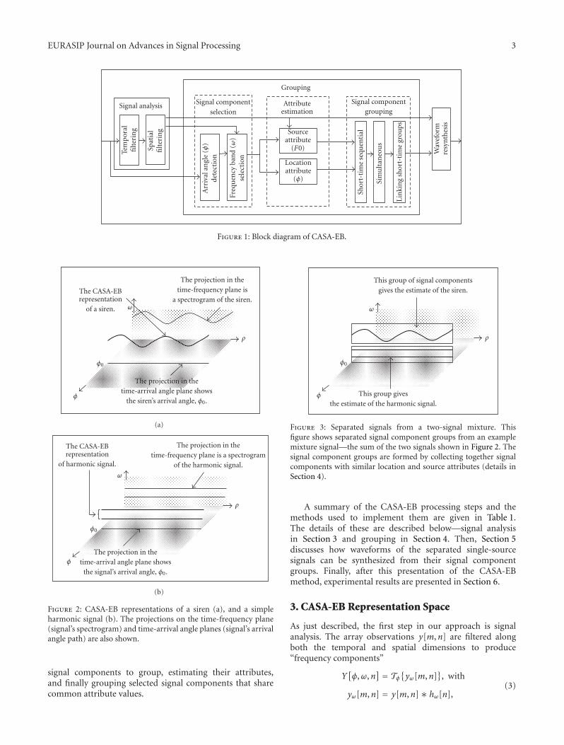
Figure 3: Separated signals from a two-signal mixture. Thisfigure shows separated signal component groups from an examplemixture signal—the sum of the two signals shown in Figure 2. Thesignal component groups are formed by collecting together signalcomponents with similar location and source attributes (details inSection 4).

A summary of the CASA-EB processing steps and themethods used to implement them are given in Table 1.The details of these are described below—signal analysisin Section 3 and grouping in Section 4. Then, Section 5discusses how waveforms of the separated single-sourcesignals can be synthesized from their signal componentgroups. Finally, after this presentation of the CASA-EBmethod, experimental results are presented in Section 6.

3. CASA-EB Representation Space

As just described, the first step in our approach is signalanalysis. The array observations y[m,n] are filtered alongboth the temporal and spatial dimensions to produce“frequency components”

Y[φ,ω,n

] = Tφ{yω[m,n]

}, with

yω[m,n] = y[m,n]∗ hω[n],(3)


Table 1: Summary of CASA-EB methods.

Processing block Method

Signal analysis

Temporal filtering Gammatone filterbank

Spatial filtering Delay-and-sum beamformer

Grouping

Signal component selection (φ) STMV beamforming

Signal component selection (ω) Signal detection using MDL criterion

Attribute estimation (F0) Autocorrelogram

Attribute estimation (φ) From P[φ,ω, ρ]

Signal component grouping (short-time sequential) Kalman filtering with Munkres’ optimal data assn algorithm

Signal component grouping (simultaneous) Clustering via a hierarchical partitioning algorithm

Signal component grouping (linking short-time groups) Munkres’ optimal data assn algorithm

Waveform resynthsis

Over frequency Adding together grouped signal components

Over time Overlap-add

where hω[n] is a bandpass temporal filter associated with thefrequency band indexed by ω, and Tφ is a spatial transformassociated with the arrival angle band indexed by φ (detailsof these signal analyses follow below).

The “frequency components” Y[φ,ω,n] are used laterin the processing (Section 4.2) for estimation of a groupingattribute, fundamental frequency, and also for waveformresynthesis. The signal components to be grouped in CASA-EB are those of its 3D representation shown in Figure 2;these are the power spectral components of the Y[φ,ω,n],obtained in the usual way as the time-average of theirmagnitudes squared

P[φ,ω, ρ

] = 1Nω

ρT+(Nω−1)/2∑

n′=ρT−(Nω−1)/2

∣∣Y[φ,ω,n′

]∣∣2, (4)

where the P[φ,ω, ρ] are downsampled from the Y[φ,ω,n]with downsampling rate T , that is, ρ = n/T , and Nω is thenumber of samples of Y[φ,ω,n] in frequency band ω thatare used to compute one sample of P[φ,ω, ρ].

3.1. Temporal Filtering. For the temporal filterbank,hω[n], ω ∈ {1, 2, . . . ,Ω}, we have used a modifiedgammatone filterbank. It consists of constant-Q filtersin high frequency bands (200 to 8000 Hz) and constant-bandwidth filters in lower frequency bands (below 200 Hz)(Constant-Q filters are a set of filters that all have the samequotient (Q), or ratio of center frequency to bandwidth.).Specifically, the constant-Q filters are the fourth-ordergammatone functions,

hω[n] = αω · e−β(αωnTs)(αωnTs)3e j2π fs/2(αωnTs)u[n], (5)

where the frequency band indices (ω = 1, 2, . . . , 75) arein reverse order, that is, the lower indices denote higherfrequencies, fs and Ts are the sampling frequency andsampling period, u[n] is the unit step function, and α and βare parameters that can be used to adjust filter characteristicssuch as bandwidths and spacing on the frequency axis. For

CASA-EB, α = 0.95, and β = 2000 work well. The constant-bandwidth filters are derived by downshifting the lowestfrequency constant-Q filter (ω = 75) by integer multiples ofits bandwidth

hω[n] = h75[n]e− j2π(ω−75)B75n, (6)

where ω = 76, 77, . . . , 90, and B75 is the bandwidth of thelowest frequency constant-Q filter.

The modified gammatone filterbank is used for temporalfiltering because it divides the frequency axis efficiently forCASA-EB. Specifically, for CASA, the frequency bands arejust narrow enough that the important spectral features ofa signal (such as harmonics in low frequencies and formantsin high frequencies) can be easily distinguished from eachother. For beamforming, the bands are narrow enough tolimit spatial filtering errors to an acceptable level.

3.2. Spatial Filtering. The spatial transform, Tφ, that we areusing is the well-known delay-and-sum beamformer

Tφ{yω[m,n]

} = 1M

M∑

m=1

yω[m,n] · e j2π(m−1) fφ , with

fφ = fωd

Csinφ,

φ ∈[−π

2, +π

2

],

(7)

where fω is the center frequency of frequency band ω, d is thedistance between adjacent microphones in a uniform lineararray, and C is the speed of sound at standard temperatureand pressure.

Delay-and-sum beamforming is used here for the sig-nal analysis in our general solution to the sound sourceseparation problem because it does not cancel correlatedsignals, for example, echos (as MV beamforming can), anddoes not require a priori information or explicit modelingof target signals, interferers, or noise (as other data adaptive


beamforming can). Its drawback is that, since it has relativelylow arrival angle resolution, each signal component willcontain more interference from neighboring arrival anglebands. In CASA-EB, this is ameliorated somewhat by theadditional separation power provided by monaural CASA.For specific applications, CASA-EB performance may beimproved by defining signal and/or noise models and usinga data adaptive beamformer.

In summary, the 3D CASA-EB representation space con-sists of signal components P[φ,ω, ρ] generated by filteringa temporally and spatially sampled input signal along bothof these dimensions (to produce frequency componentsY[φ,ω,n]), and then, taking the average magnitude squaredof these.

4. CASA-EB Grouping to SeparateSingle-Source Signals

As described previously, the second step in CASA-EB isto group signal components from the time-frequency-arrival angle space into separated single-source signal esti-mates. Grouping consists of three steps: selecting the signalcomponents for grouping, estimating their location andsource attributes, and finally, grouping those with similarlyvalued attributes to form the separated single-source signalestimates. The details of these three steps are given in thefollowing three subsections.

4.1. Signal Component Selection. In this step, the set of allsignal components (P[φ,ω, ρ]) is pruned to produce a subsetof “significant” signal components, which are more likelyto have come from actual sound sources of interest andto constitute the main part of their signals. Grouping isthen performed using only this subset of signals. Experienceand experimental results indicate that this type of before-grouping pruning does not adversely affect performance andhas the following two benefits. First, it reduces the com-putational complexity of grouping and second, it increasesgrouping robustness (since there are fewer spurious signalcomponents to throw the grouping operation “off-track”).Now, we describe the signal component selection process inmore detail.

4.1.1. Arrival Angle Detection. This process begins withpruning away signal components from arrival angles inwhich it is unlikely there is any andible target sound, thatis, from angles within which the signal power is low. Thereare a variety of ways to detect such low-power arrival angles.For example, a simple way is, for a given time frame ρ, to addup the power spectral components P[φ,ω, ρ] in each arrivalangle band φ

P[φ] =

∑

ω

P[φ,ω, ρ

]. (8)

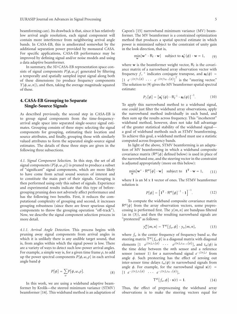
In this work, we are using a wideband adaptive beam-former by Krolik—the steered minimum variance (STMV)beamformer [14]. This wideband method is an adaptation of

Capon’s [15] narrowband minimum variance (MV) beam-former. The MV beamformer is a constrained optimizationmethod that produces a spatial spectral estimate in whichpower is minimized subject to the constraint of unity gainin the look direction, that is,

minw

[w+ · Rf ·w] subject to a+f

(φ) ·w = 1, (9)

where w is the beamformer weight vector, Rf is the covari-ance matrix of a narrowband array observation vector withfrequency f , + indicates conjugate transpose, and af (φ) =[1 e− j2π f t1(φ) · · · e− j2π f tM−1(φ)]

Tis the “steering vector.”

The solution to (9) gives the MV beamformer spatial spectralestimate:

Pf[φ] = [a+

f

(φ) · R−1

f · af(φ)]−1

. (10)

To apply this narrowband method to a wideband signal,one could just filter the wideband array observations, applythe narrowband method individually in each band, andthen sum up the results across frequency. This “incoherent”wideband method, however, does not take full advantageof the greater statistical stability of the wideband signal—a goal of wideband methods such as STMV beamforming.To achieve this goal, a wideband method must use a statisticcomputed across frequency bands.

In light of the above, STMV beamforming is an adapta-tion of MV beamforming in which a wideband compositecovariance matrix (Rst[φ] defined below) is used in place ofthe narrowband one, and the steering vector in the constraintis adjusted appropriately (more on this below):

minw

[w+ · Rst

[φ] ·w

]subject to 1T ·w = 1, (11)

where 1 is an M x 1 vector of ones. The STMV beamformersolution is

P[φ] =

[1T · Rst

[φ]−1 · 1

]−1. (12)

To compute the wideband composite covariance matrixRst[φ] from the array observation vectors, some prepro-cessing is performed first. The y[m,n] are bandpass filtered(as in (3)), and then the resulting narrowband signals are“presteered” as follows:

ystω [m,n] = Tst

[fω,φ

] · yω[m,n], (13)

where fω is the center frequency of frequency band ω, thesteering matrix Tst[ fω,φ] is a diagonal matrix with diagonal

elements [1 e j2π fωt1(φ) · · · e j2π fωt(M−1)(φ)], and tm(φ) isthe time delay between the mth sensor and a referencesensor (sensor 1) for a narrowband signal e− j2π fωt fromangle φ. Such presteering has the effect of zeroing outinter-sensor time delays tm(φ) in narrowband signals fromangle φ. For example, for the narrowband signal s(t) =[1 e− j2π fωt1(φ) · · · e− j2π fωtM−1(φ)],

Tst[fω,φ

] · s(t) = 1. (14)

Thus, the effect of preprocessing the wideband arrayobservations is to make the steering vectors equal for


all frequency bands (afω(φ) = 1), and this provides afrequency-independent steering vector to use in the STMVbeamformer’s unity-gain constraint.

Now, given the presteered array observations, the wide-band composite covariance matrix is simply

Rst[φ] =

h∑

ω=l

n0+(N−1)∑

n=n0

ystω [m,n] · yst+

ω [m,n],

=h∑

ω=lTst[fω,φ

] · Rω ·Tst+[fω,φ

],

(15)

where Rω is the covariance matrix of yω[m,n], and thesummations run from frequency band l to h and from timeindex n0 to n0 + (N − 1).

The advantage of Krolik’s technique over that of (8) andother similar data-independent beamforming techniques isthat it provides higher arrival angle resolution. Comparedto other data adaptive methods, it does not require a prioriinformation about the source signals and/or interference,does not cancel correlated signals (as MV beamforming isknown to do), and is not vulnerable to source location bias(as other wideband adaptive methods, such as the coherentsignal-subspace methods, are [16]).

4.1.2. Frequency Band Selection. Now, for each detectedarrival angle band, φ0, the next step is to select the significantsignal components from that arrival angle band. This isdone in two steps. First, high-power signal componentsare detected, and low-power ones pruned. Then, the high-power components are further divided into peaks (i.e.,local maxima) and their neighboring nonpeak components.Although all the high-power components will be includedin the separated signals, only the peak components need tobe explicitly grouped. Due to the nature of the gammatonefilterbank we are using, the non-peak components can beadded back into the separated signal estimates later at signalreconstruction time, based on their relationship with a peak.Consider the following. Since the filterbank’s neighboringfrequency bands overlap, a high-power frequency compo-nent sufficient to generate a peak in a given band is also likelyto contribute significant related signal power in neighboringbands (producing non-peak components). Thus, these non-peak components are likely to be generated by the samesignal feature as their neighboring peak, and it is reasonableto associate them.

Low-power signal components are detected and prunedusing a technique by Wax and Kailath [17]. In their work,a covariance matrix is computed from multichannel inputdata, and its eigenvalues are sorted into a low-power set(from background noise) and a high-power set (fromsignals). The sorting is accomplished by minimizing aninformation theoretic criterion, such as Akaike’s InformationCriterion (AIC) [18, 19] or the Minimum DescriptionLength (MDL) criterion [20, 21]). The MDL is discussed here

since it is the one used in CASA-EB. From [17], it is definedas

MDL = − log

⎛⎝ ΠL

i=λ+1l1/(L−λ)i

(1/(L− λ)) ·∑Li=λ+1 li

⎞⎠

(L−λ)Nt

+12λ(2L− λ) logNt,

(16)

where λ ∈ {0, 1, . . . ,L − 1} is the number of possiblesignal eigenvalues and the parameter over which the MDLis minimized, L is the total number of eigenvalues, li is theith largest eigenvalue, and Nt is the number of time samplesof the observation vectors used to estimate the covariancematrix. The λ that minimizes the MDL (λmin) is the estimatednumber of signal eigenvalues, and the remaining (L −λmin) smallest eigenvalues are the detected noise eigenvalues.Notice, this MDL criterion is entirely a function of the(L − λ) smallest eigenvalues, and not the larger ones.Thus, in practice, it distinguishes between signal and noiseeigenvalues based on the characteristics of the backgroundnoise. Specifically, it detects a set of noise eigenvalues withrelatively low and approximately equal power. Wax andKailath use this method to estimate the number of signalsin multichannel input data. We use it to detect and removethe (L − λmin) low-power, noise components P[φ,ω, ρ]—bytreating the P[φ,ω, ρ] as the eigenvalues in their method.We chose this method for noise detection because it worksbased on characteristics of the noise, rather than relying onarbitrary threshold setting.

In summary, signal component selection/pruning isaccomplished in two steps. For each fixed time frameρ, high power arrival angle bands are detected, and sig-nal components from low power arrival angle bands areremoved. Then, in high power arrival angle bands, low-power signal components are removed and high-powersignal components are divided into peaks (for grouping)and non-peaks (to be added back into the separated signalestimates after grouping, at signal reconstruction time).

4.2. Attribute Estimation. In the previous section, wedescribed how signal components in the CASA-EB repre-sentation can be pruned and selected for grouping. In thissection, we describe how to estimate the selected signalcomponents’ attributes that will be used to group them.In this work, we estimate two types of signal attributes,location attributes and source attributes. As described in theintroduction, these are complementary. Used together, theymay allow more types of sound mixtures to be separated andproduce more completely separated source signals.

4.2.1. Locaton Attribute. For a selected signal component,P[φ,ω, ρ], the location attribute used in CASA-EB is itsarrival angle band, or simply its φ index. This is the delay-and-sum beamformer steering angle from the spatial filteringstep in Section 3.

4.2.2. Source Attribute. Source attributes are features embed-ded in a signal that describe the state of the signal’s source


at the time it produced the signal. In the previous work,several different source attributes have been used, includingF0 [2, 3, 8–11, 22, 23], amplitude modulation [8], onset time[9, 23], offset time [9], and timbre [24]. In this work, we usean F0 attribute. Since F0 is the most commonly used, its usehere will allow our results to be compared to those of othersmore easily. Next, we discuss F0 estimation in more detail.

There are two main approaches to F0 estimation: spectralpeak-based and autocorrelation-based methods. The spectralpeak-based approach is straightforward when there is onlyone harmonic group in the sound signal. In this case, itdetects peaks in the signal’s spectrum and estimates F0 byfinding the greatest common divisor of their frequencies.However, complications arise when the signal containsmore than one harmonic group. Specifically, there is theadded “data association problem,” that is, the problem ofdetermining the number of harmonic groups and whichspectral peaks belong to which harmonic groups. Theautocorrelation-based approach handles the data associationproblem more effectively and furthermore, as indicated in[25], also provides more robust F0 estimation performance.Hence, an autocorrelation-based method is used in thiswork.

The basic idea behind the autocorrelation method is thata periodic signal will produce peaks in its autocorrelationfunction at integer multiples of its fundamental period, andthese can be used to estimate F0. To use F0 as an attributefor grouping signal components, however, it is also necessaryto be able to associate the signal components P[φ,ω, ρ] withthe F0 estimates. This can be done using an extension of theautocorrelation method—the autocorrelogram method.

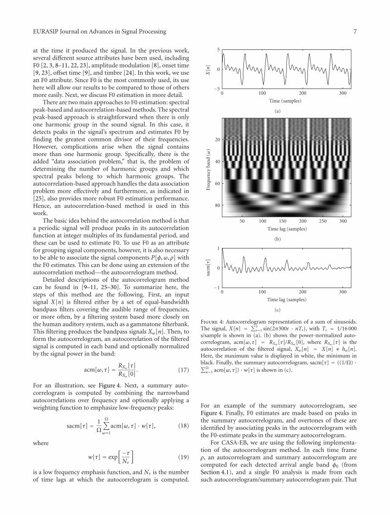
Detailed descriptions of the autocorrelogram methodcan be found in [9–11, 25–30]. To summarize here, thesteps of this method are the following. First, an inputsignal X[n] is filtered either by a set of equal-bandwidthbandpass filters covering the audible range of frequencies,or more often, by a filtering system based more closely onthe human auditory system, such as a gammatone filterbank.This filtering produces the bandpass signals Xω[n]. Then, toform the autocorrelogram, an autocorrelation of the filteredsignal is computed in each band and optionally normalizedby the signal power in the band:

acm[ω, τ] = RXω[τ]RXω[0]

. (17)

For an illustration, see Figure 4. Next, a summary auto-correlogram is computed by combining the narrowbandautocorrelations over frequency and optionally applying aweighting function to emphasize low-frequency peaks:

sacm[τ] = 1Ω

Ω∑

ω=1

acm[ω, τ] ·w[τ], (18)

where

w[τ] = exp[−τNτ

](19)

is a low frequency emphasis function, and Nτ is the numberof time lags at which the autocorrelogram is computed.

−5

0

5

X[n

]

0 100 200 300

Time (samples)

(a)

80

60

40

20

Freq

uen

cyba

nd

(ω)

50 100 150 200 250 300

Time lag (samples)

(b)

−1

0

1

sacm

[τ]

0 100 200 300

Time lag (samples)

(c)

Figure 4: Autocorrelogram representation of a sum of sinusoids.The signal, X[n] = ∑5

r=1 sin(2π300r · nTs), with Ts = 1/16 000s/sample is shown in (a). (b) shows the power-normalized auto-correlogram, acm[ω, τ] = RXω [τ]/RXω [0], where RXω [τ] is theautocorrelation of the filtered signal, Xω[n] = X[n] ∗ hω[n].Here, the maximum value is displayed in white, the minimum inblack. Finally, the summary autocorrelogram, sacm[τ] = ((1/Ω) ·∑Ω

ω=1 acm[ω, τ]) ·w[τ] is shown in (c).

For an example of the summary autocorrelogram, seeFigure 4. Finally, F0 estimates are made based on peaks inthe summary autocorrelogram, and overtones of these areidentified by associating peaks in the autocorrelogram withthe F0-estimate peaks in the summary autocorrelogram.

For CASA-EB, we are using the following implementa-tion of the autocorrelogram method. In each time frameρ, an autocorrelogram and summary autocorrelogram arecomputed for each detected arrival angle band φ0 (fromSection 4.1), and a single F0 analysis is made from eachsuch autocorrelogram/summary autocorrelogram pair. That


is, for each φ0, an autocorrelogram and summary autocor-relogram are computed from the temporally and spatiallyfiltered signal, Y[φ0,ω,n], ω ∈ {1, 2, . . . ,Ω} and n ∈ {ρT −Nτ/2+1, . . . , ρT+Nτ/2}, where we usedNτ = 320 (equivalentto 20 milliseconds). Then, for this arrival angle band andtime frame, the F0 estimation method of Wang and Brown[11] is applied, producing a single F0 estimate made fromthe highest peak in the summary autocorrelogram

F̂0[φ0, ρ

], (20)

and a set of flags, indicating for each P[φ0,ω, ρ], whether itcontains a harmonic of F̂0[φ0, ρ] or not

FN[φ0,ω, ρ

], ω ∈ {1, 2, . . . ,Ω}. (21)

Here, FN[φ0,ω, ρ] = 1 when band ω contains a harmonic,and 0 otherwise. Details of the implementation are thefollowing.

Temporal filtering is done with a gammatone filterbankbecause its constant-Q filters can resolve important low-frequency features of harmonic signals (the fundamental andits lower frequency harmonics) better than equal-bandwidthfilterbanks with the same number of bands (Low frequencyharmonics are important since, in speech for example, theyaccount for much of the signal power in vowels). Thesebetter-resolved, less-mixed low frequency harmonics cangive better F0 estimation results (F0 estimates and relatedharmonic flags, FN’s), since they produce sharper peaks inthe autocorrelogram, and these sharper peaks are easier forthe F0 estimation algorithm to interpret. Spatial filtering(new to autocorrelogram analysis) is used here becauseit provides the advantage of reducing interference in theautocorrelogram when multiple signals from different spatiallocations are present in the input.

The autocorrelogram is computed as described pre-viously, including the optional power normalization ineach frequency band. For the summary autocorrelogram,however, we have found that F0 estimation is improvedby using just the lower frequency bands that contain thestrongest harmonic features. Thus,

sacm[τ] = 174

90∑

ω=17

acm[ω, τ] ·w[τ], (22)

where the bands, 90 to 17, cover the frequency range, 0, to3500 Hz, the frequency range of a vowel’s fundamental andits lower harmonics.

Finally, an F0 analysis is performed using the autocor-relogram/summary autocorrelogram pair, according to themethod of Wang and Brown [11]. Their method is usedin CASA-EB to facillitate comparison testing of CASA-EB’Smonaural CASA to their monaural CASA (described inSection 6). The details of the method are the following. First,a single F0 is estimated based on the highest peak in thesummary autocorrelogram:

F̂0[φ0, ρ

] = fsτm

, (23)

where fs is the temporal sampling frequency of the inputsignal y[m,n], and τm is the time lag of the highest peakin the summary autocorrelogram. Then, the associatedovertones of this F0 are identified by finding frequencybands in the autocorrelogram with peaks at, or near, τm.Specifically, this is done as follows. A band ω is determinedto contain an overtone, that is, FN[φ0,ω, ρ] = 1, when

RXω[τm]RXω[0]

> Θd, (24)

and Θd = 0.90 is a detection threshold. Wang and Brownused Θd = 0.95. For CASA-EB, experiments show thatΘds in the range of 0.875 to 0.95 detect overtones well[31]. This F0 estimation method amounts to estimatingF0 and detecting its overtones for a single “foregroundsignal,” and treating the rest of the input mixture signalas background noise and interference. Although this limitsthe number of signals for which an F0 estimate is made(one per autocorrelogram), it also helps by eliminating theneed to estimate the number of harmonic signals. Further,it provides more robust F0 estimation since, from eachautocorrelogram, an F0 estimate is only made from the signalwith the strongest harmonic evidence (the highest peak inthe summary autocorrelogram).

Notice that in our application, the number of signals forwhich F0 estimates can be made is less limited since we havemore than one autocorrelogram per time frame (one for eachdetected arrival angle). Additionally, our F0 estimates maybe better since they are made from autocorrelograms withless interharmonic group interference. Such interference isreduced since the autocorrelograms are computed from thespatially filtered signals, Y[φ0,ω,n], ω ∈ {1, 2, . . . ,Ω}, thatare generally “less mixed” than the original input mixturesignal y[m,n] because they contain a smaller number ofharmonic groups with significant power.

4.3. Signal Component Grouping. Recall that sound sourceseparation consists of two steps: signal analysis (to breakthe signal into components such as P[φ,ω, ρ]), and signalcomponent grouping (to collect the components into singlesource signal estimates). Grouping collects together signalcomponents according to their attributes (estimated inSection 4.2), and ideally, each group only contains piecesfrom a single source signal.

Grouping is typically done in two stages: simultaneousgrouping clusters together signal components in each timeframe ρ that share common attribute values, and sequentialgrouping tracks these simultaneous groups across time. Inthe previous work, many researchers perform simultaneousgrouping first and then track the resulting clusters [2, 3, 10,22, 32]. For signals grouped by the F0 source attribute, forexample, the simultaneous grouping step consists of iden-tifying groups of harmonics, and the sequential groupingstep consists of tracking their fundamental frequencies. Aprimary advantage of simultaneous-first grouping is that itcan be real-time amenable when the target signals’ modelsare known a priori. However, when they are not known, itcan be computationally complex to determine the correct


signal models [10], or error-prone if wrong signal models areused.

Some researchers have experimented with sequential-first grouping [8, 9]. In this case, the sequential grouping stepconsists of tracking individual signal components, and thesimultaneous grouping step consists of clustering togetherthe tracks that have similar source attribute values in thetime frames in which they overlap. Although this approachis not real-time amenable since tracking is performed on thefull length of the input mixture signal before the resultingtracks are clustered, it has the advantage that it controlserror propagation. It does this by putting off the more error-prone decisions (simultaneous grouping’s signal modelingdecisions) until later in the grouping process.

In this work, we strike a balance between the twowith a short-time sequential-first grouping approach. Thisis a three-step approach (illustrated in Figure 5). First, toenjoy the benefits of sequential-first grouping (reducederror-propagation) without suffering long time delays, westart by tracking individual signal components over a fewframes. Then, these short-time frequency component tracksare clustered together into short-time single-source signalestimates. Finally, since signals are typically longer than afew frames, it is necessary to connect the short-time signalestimates together (i.e., to track them). The details of thesethree steps are given next.

4.3.1. Short-Time Sequential Grouping. In this step, signalcomponents are tracked for a few frames (six for the resultspresented in this paper). Recall from Section 4.1 that thesignal components that are tracked are the perceptuallysignificant ones (peak, high-power components from arrivalangle bands in which signals have been detected). Limitingtracking to these select signal components reduces computa-tional complexity and improves tracking performance.

Technically, tracking amounts to estimating the state of atarget (e.g., its position and velocity) over time from relatedobservation data. A target could be an object, a system, ora signal, and a sequence of states over time is called a track.In our application, a target is a signal component of a singlesound source’s signal (e.g., the nth harmonic of a harmonicsignal), its state consists of parameters (e.g., its frequency)that characterize the signal component, and the observationdata in each frame ρ consists of the (multi source) signalcomponents P[φ,ω, ρ].

Although we are tracking multiple targets (signal com-ponent sequences), for the sake of simplicity, we firstconsider the tracking of a single target. In this case, awidely used approach for tracking is the Kalman filter [33].This approach uses a linear system model to describe thedynamics of the target’s internal state and observable output,that is,

x[ρ + 1

] = A[ρ] · x

[ρ]

+ v[ρ],

z[ρ + 1

] = C[ρ + 1

] · x[ρ + 1

]+ w

[ρ + 1

].

(25)

Here, x[ρ+1] is the target’s state and z[ρ+1] is its observableoutput in time frame (ρ + 1), A[ρ] is the state transitionmatrix, C[ρ + 1] is the matrix that transforms the current

2signal

estimates

3 short-timesequential groups

(tracks)

ρ

η (η + 1)

ω

(a)

2signal

estimates

2 short-timegroups

ρ

ω

(b)

2 signalestimates

through framesequence η + 1

ρ

ω

(c)

Figure 5: Illustration of short-time sequential-first grouping. Herethe input signal is a mixture of the two single-source signals shownin Figure 2. (a) The graph shows short-time tracks in time segment(η+1) with completed signal estimate groups through time segmentη. Here, time segment η consists of time frames ρ ∈ {ηT ′, . . . , (η +1)T ′ −1}, and T ′ = 6. (b) The graph shows simultaneous groups ofthe short-time tracks shown in (a). (c) The graph shows completedsignal estimate groups through time segment (η + 1).

state of the track to the output, and v[ρ] and w[ρ] are zero-mean white Gaussian noise with covariance matrices Q[ρ]and R[ρ], respectively. Based on this model, the Kalman filteris a set of time-recursive equations that provides optimalstate estimates. At each time (ρ + 1), it does this in twosteps. First, it computes an optimal prediction of the statex[ρ + 1] from an estimate of the state x[ρ]. Then, thisprediction is updated/corrected using the current outputz[ρ + 1], generating the final estimate of x[ρ + 1].

Since the formulas for Kalman prediction and update arewell known [33], the main task for a specific applicationis reduced to that of constructing the linear model, that is,defining the dynamic equations (see (25)). For CASA-EB, atarget’s output vector, z[ρ], is composed of its frequency andarrival angle bands, and its internal state, x[ρ], consists of itsfrequency and arrival angle bands, along with their rates ofchange:

z[ρ] = [φ ω

]T ,

x[ρ] =

[φ

d

dtφ ω

d

dtω]T.

(26)


The transition matrices of the state and output equations aredefined as follows:

A[ρ] =

⎡⎢⎢⎢⎢⎢⎢⎣

1 0 0 0

0 1 0 0

0 0 1 0

0 0 0 1

⎤⎥⎥⎥⎥⎥⎥⎦

,

C[ρ] =

⎡⎣

1 0 0 0

0 0 1 0

⎤⎦,

(27)

where this choice of A[ρ] reflects our expectation that thestate changes slowly, and this C[ρ] simply picks the outputvector ([φ ω]T) from the state vector.

When there is more than one target, the tracking problembecomes more complicated. Specifically, at each time instant,multiple targets can produce multiple observations, andgenerally, it is not known which target produced whichobservation. To solve this problem, a data association processis usually used to assign each observation to a target. Then,Kalman filtering can be applied to each target as in the singletarget case.

While a number of data association algorithms have beenproposed in the literature, most of them are based on thesame intuition—that an observation should be associatedwith the target most likely to have produced it (e.g., the“closest” one). In this work, we use an extension of Munkres’optimal data association algorithm (by Burgeois and Lassalle[34]). A description of this algorithm can be found in [35].To summarize briefly here, the extended Munkres algorithmfinds the best (lowest cost) associations of observations toestablished tracks. It does this using a cost matrix with Hcolumns (one per observation) and J+H rows (one per trackplus one per observation), where the ( j,h)th element is thecost of associating observation h to track j, the (J + h,h)th

element is the cost of initiating a new track with observationh, and the remaining off-diagonal elements in the final Hrows are set to a large number such that they will not affectthe result.

The cost of associating an observation with a track is afunction of the distance between the track’s predicted nextoutput and the observation. Specifically, we are using thefollowing distance measure:

cost j,h =

⎧⎪⎨⎪⎩

∣∣∣ω̂ j − ωh∣∣∣, when

∣∣∣ω̂ j − ωh∣∣∣ ≤ 1 and φh = φj ,

2γ, otherwise,

(28)

where ω̂ j is the prediction of track j’s next frequency (ascomputed by the Kalman filter), ωh and φh are the frequencyand arrival angle of observation h, respectively, and track j’sarrival angle band φj is constant. Finally, γ is an arbitrarylarge number used here so that if observation h is outsidetrack j’s validation region, (|ω̂ j − ωh| > 1 or φh /=φj),then observation h will not be associated with track j. Notethat this cost function means that frequency tracks changetheir frequency slowly (≤1 freqency band per time frame),

and sound sources do not move (since φj is held constant).In subsequent work, the assumption of unmoving sourcescould be lifted by revising the cost matrix and makingadjustments to the simultaneous grouping step (describednext in Section 4.3.2).

Finally, the cost of initiating a new track is simply set tobe larger than the size of the validation region

costJ+h,h = γ, (29)

and the remaining costs in the last H rows are set equal to 2γso that they will never be the low cost choice.

4.3.2. Simultaneous Grouping. In this step, the short-timetracks from the previous step are clustered into short-timesignal estimates based on the similarity of their source andlocation attribute values. There are a variety of clusteringmethods in the literature (refer to pattern recognition texts,such as [36–40]). In CASA-EB, we use the hierarchicalpartitioning algorithm that is summarized next.

Partitioning is an iterative approach that divides ameasurement space into k disjoint regions, where k is apredefined input to the partitioning algorithm. In general,however, it is difficult to know k a priori. Hierarchicalpartitioning addresses this issue by generating a hierarchy ofpartitions—over a range of different k values—from whichto choose the “best” partition. The specific steps are thefollowing. (1) Initialize k to be the minimum number ofclusters to be considered. (2) Partition the signal componenttracks into k clusters. (3) Compute a performance measureto quantify the quality of the partition. (4) Increment k by 1and repeat steps 2–4, until a stopping criterion is met, or kreaches a maximum value. (5) Select the best partition basedon the performance measure computed in step 3.

To implement the hierarchical partitioning algorithm,some details remain to be determined: the minimumand maximum number of clusters to be considered, thepartitioning algorithm, the performance measure, and aselection criterion to select the best partition based onthe performance measure. For CASA-EB, we have madethe following choices. For the minimum and maximumnumbers of clusters, we use the number of arrival anglebands in which signals have been detected, and the totalnumber of arrival angle bands, respectively.

For partitioning algorithms, we experimented with adeterministic one, partitioning around medoids (PAMs), anda probabilistic one, fuzzy analysis (FANNY)—both froma statistics shareware package called R [41, 42]. (R is areimplementation of S [43, 44] using Scheme semantics. Sis a very high level language and an environment for dataanalysis and graphics. S was written by Richard Becker,John M. Chambers, and Allan R. Wilks of AT&T BellLaboratories Statistics Research Department.) The differencebetween the two is in how measurements are assigned toclusters. PAM makes hard clustering assignments; that is,each measurement is assigned to a single cluster. FANNY,on the other hand, allows measurements to be spread acrossmultiple clusters during partitioning. Then, if needed, thesefuzzy assignments can be hardened at the end (after the last


iteration). For more information on PAM and FANNY, referto [37]. For CASA-EB, we use FANNY since it producesbetter clusters in our experiments.

Finally, it remains to discuss performance measures andselection criteria. Recall that the performance measure’spurpose in hierarchical partitioning is to quantify the qualityof each partition in the hierarchy. Common methods fordoing this are based on “intracluster dissimilarities” betweenthe members of each cluster in a given partition (smallis good), and/or on “intercluster dissimilarities” betweenthe members of different clusters in the partition (large isgood). As it turns out, our data produces clusters that areclose together. Thus, it is not practical to seek clusters withlarge inter-cluster dissimilarities. Rather, we have selected aperformance measure based on intra-cluster dissimilarities.Two intra-cluster performance measures were considered:the maximum intra-cluster dissimilarity in any single clusterin the partition, and the mean intra-cluster dissimilarity(averaged over all clusters in the partition). The maximumintra-cluster dissimilarity produced the best partitions forour data and is the one we used. The details of thedissimilarity measure are discussed next.

Dissimilarity is a measure of how same/different twomeasurements are from each other. It can be computed ina variety of ways depending on the measurements beingclustered. The measurements we are clustering are the sourceand location attribute vectors of signal component tracks.Specifically, for each short-time track j in time segment η,this vector is composed of the track’s arrival angle band φj ,and its F0 attribute in each time frame ρ of time segment ηin which the track is active. Recall (from Section 4.2), this F0attribute is the flag FN[φj ,ωj[ρ], ρ] that indicates whetherthe track is part of the foreground harmonic signal or not, intime frame ρ. Here, ρ ∈ {ηT′, . . . , (η + 1)T′ − 1}, T′ is thenumber of time frames in short-time segment η, and ωj[ρ]is track j’s frequency band in time frame ρ.

Given this measurement vector, dissimilarity is computedas follows. First, since we do not want to cluster tracks fromdifferent arrival angles, if two tracks ( j1 and j2) have differentarrival angles, their dissimilarity is set to a very large number.Otherwise, their dissimilarity is dependent on the differencein their F0 attributes in the time frames in which they areboth active

dj1, j2 =∑(η+1)T′−1

ρ=ηT′ D ·wj1, j2

[ρ]

∑(η+1)T′−1ρ=ηT′ wj1, j2

[ρ] , (30)

where D denotes |FNj1 [φj1 ,ωj1 [ρ], ρ]− FNj2 [φj2 ,ωj2 [ρ], ρ]|and wj1, j2 [ρ] is a flag indicating whether tracks j1 and j2 areboth active in time frame ρ, or not:

wj1, j2

[ρ] =

⎧⎪⎪⎪⎪⎨⎪⎪⎪⎪⎩

1, if tracks, j1 and j2,

are both active in time frame ρ,

0, otherwise.

(31)

If there are no time frames in which the pair of tracks areboth active, it is not possible to compute their dissimilarity.

In this case, dj1, j2 is set to a neutral value such that their(dis)similarity will not be a factor in the clustering. Sincethe maximum dissimilarity between tracks is 1 and theminimum is 0, the neutral value is 1/2. For such a pair oftracks to be clustered together, they must each be close to thesame set of other tracks. Otherwise, they will be assigned todifferent clusters.

Now that we have a performance measure (maximumintra-cluster dissimilarity), how should we use it to selecta partition? It may seem reasonable to select the onethat optimizes (minimizes) the performance measure. Thisselection criterion is no good though; it selects a partitionin which each measurement is isolated in a separate cluster.A popular strategy used in hierarchical clustering is to picka partition based on changes in the performance measure,rather than on the performance measure itself [37, 38,40]. For CASA-EB, we are using such a selection criterion.Specifically, in keeping with the nature of our data (whichcontains a few, loosely connected clusters), we have chosenthe following selection criterion. Starting with the minimumnumber of clusters, we select the first partition (the onewith the smallest number of clusters, k) for which thereis a significant change in performance from the previouspartition (with (k − 1) clusters).

4.3.3. Linking Short-Time Signal Estimate Groups. This isthe final grouping step. In the previous steps, we havegenerated short-time estimates of the separated sourcesignals (clusters of short-time signal component tracks). Inthis step, these short-time signal estimates will be linkedtogether to form full-duration signal estimates. This is adata association problem. The short-time signal estimates ineach time segment η must be associated with the previouslyestablished signal estimates through time segment (η − 1).For an illustration, see Figure 5. To make this association,we rely on the fact that signals usually contain some longsignal component tracks that continue across multiple timesegments. Thus, these long tracks can be used to associateshort-time signal estimates across segments. The idea is thata signal estimate’s signal component tracks in time segment(η − 1) will contine to be in the same signal in time segmentη, and similarly, signal component tracks in a short-timesignal estimate in time segment η will have their origins inthe same signal in preceeding time segments. The details ofour processing are described next.

For this data association problem, we use the extendedMunkres algorithm (as described in Section 4.3.1) with acost function that is based on the idea described previously.Specifically, the cost function is the following:

costgk[ρ],c�[η] =Ak,� −Bk,�

Ak,�, (32)

where gk[ρ] is the kth signal estimate through the (η− 1)st

time segment (i.e., ρ < ηT′), c�[η] is the �th short-time signalestimate in time segment η, Ak,� is the power in the union ofall their frequency component tracks,

Ak,� =∑

j∈{gk[ρ]∪c�[η]}P j , (33)


P j is the power in track j (defined below), Bk,� is the powerin all the frequency component tracks that are in both gk[ρ]and c�[η],

Bk,� =∑

j∈{gk[ρ]∩c�[η]}P j , (34)

and P j is computed by summing all the power spectraldensity components along the length of track j,

P j =min((η+1)T′−1, jstop)∑

ρ= jstart

P[φj ,ωj

[ρ], ρ]. (35)

This cost function takes on values in the range of 0 to 1.The cost is 0 when all the tracks in cluster c�[η] that havetheir beginning in an earlier time sequence are also in clustertrack gk[ρ], and vice versa. The cost is 1 when c�[η] and gk[ρ]do not share any of the same signal component tracks.

Finally, notice that this cost function does not treat alltracks equally; it gives more weight to longer and morepowerful tracks. To see this, consider two clusters: c�1 [η] andc�2 [η] that each contains one shared track with gk[ρ]. Let theshared track in c�1 [η] be long and have high power, and letthe shared track in c�2 [η] be short and have low power. Then,Bk,1 will be larger than Bk,2, and thus costk,1[η] < costk,2[η].Although both c�1 [η] and c�2 [η] have one continuing tracksegment from gk[ρ], the one with the longer, stronger sharedtrack is grouped with it. In this way, the cost function favorssignal estimates that keep important spectral structuresintact.

5. CASA-EB Waveform Synthesis

The preceeding processing steps complete the separation ofthe mixture signal into the single-source signal estimatesgk[ρ]. However, the signal estimates are still simply groups ofsignal components. In some applications, it may be desirableto have waveforms (e.g., to listen to the signal estimates, or toprocess them further in another signal processing applicationsuch as an automatic speech recognizer).

Waveform reconstruction is done in two steps. First,in time frame ρ, a short-time waveform is generated foreach group, gk[ρ], that is active (i.e., nonempty) in thetime frame. Then, full-length waveforms are generated fromthese by connecting them together across time frames. Theimplementation details are described next.

In the first step, for each currently active group, itsshort-time waveform is generated by summing its short-timenarrowband waveforms Y[φ,ω,n] over frequency:

x̂ρk[n] =

∑

φ,ω s.t.

P[φ,ω,ρ]∈gk[ρ]

Y[φ,ω,n

],

(36)

where n ∈ {ρ−(T−1)/2 · · · ρ+(T−1)/2}. In the second step,these short-time waveforms are connected together acrosstime into full-length waveforms by the standard overlap-addalgorithm,

x̂k[n] =∑

ρ

(T−1)/2∑

r=−(T−1)/2

v[r] · x̂ρk[r], (37)

where we have chosen to use a Hanning window, v[·],because of its low sidelobes and reasonably narrow main lobewidth.

6. Experimental Results

For a sound source separation method, such as CASA-EB, it is important that it both separate mixture signalscompletely and that the separated signals have good quality.The experiments described in Section 6.2 assess CASA-EB’sability to do these. Specifically, they test our hypothesis thatcombining monaural CASA and beamforming, as in CASA-EB, provides more complete signal separation than eitherCASA or beamforming alone, and that the separated signalshave low spectral distortion.

Before conducting these experiments, a preliminaryexperiment is performed. In particular, to make the com-parison of CASA-EB to monaural CASA meaningful, first weneed to verify that the performance of the monaural CASAin CASA-EB is inline with other previously published CASAmethods. Since it is not practical to compare our CASAtechnique to every previously proposed technique (thereare too many and there is no generallyaccepted standard),we selected a representative technique for comparison—thatof van der Kouwe, Wang and Brown [1]. We chose theirmethod for three reasons. First, a clear comparison canbe made since their testing method is easily reproduciblewith readily-available test data. Second, comparison to theirtechnique can provide a good check for ours since thetwo methods are similar; they both use the same groupingcue and a similar temporal analysis filter, hω[n]. The maindifferences are that our technique contains spatial filtering(which theirs does not), and it uses tracking/clusteringfor grouping (while their technique uses neural networksfor grouping). Finally, they (Roman, Wang and Brown)have also done work separating signals based on locationcues (binaural CASA) [4], and some preliminary workcombining source attributes (F0 attribute) and locationattributes (binaural CASA cues)—see [13] by Wrigley andBrown.

6.1. Preliminary Signal Separation Experiments: MonauralCASA. To compare our monaural CASA technique to thatof [1], we tested our technique using the same test dataand performance measure as they used to test theirs. Inthis way, our results can be compared directly to theirpublished results. The test data consists of 10 mixturesignals from the data set of [8]. Each mixture consists of aspeech signal (v8) and one of ten interference signals (seeTable 2).

The performance measure is the SIR gain (signal tointerference ratio) (this SIR gain is the same as the SNR gainin [1]; we prefer the name SIR gain since it is a more accuratedescription of what is computed), that is, the differencebetween the SIRs before and after signal separation:

ΔSIR = SIRafter − SIRbefore, (38)


−10

0

10

20

30

40

50

60SI

Rga

in(d

B)

0 1 2 3 4 5 6 7 8 9

Index of interferer (n0–n9)

(a)

−10

0

10

20

30

40

50

60

SIR

gain

(dB

)

0 1 2 3 4 5 6 7 8 9


(b)

−10

0

10

20

30

40

50

60

SIR

gain

(dB

)

0 1 2 3 4 5 6 7 8 9


SIR beforeSIR afterSIR gain

(c)

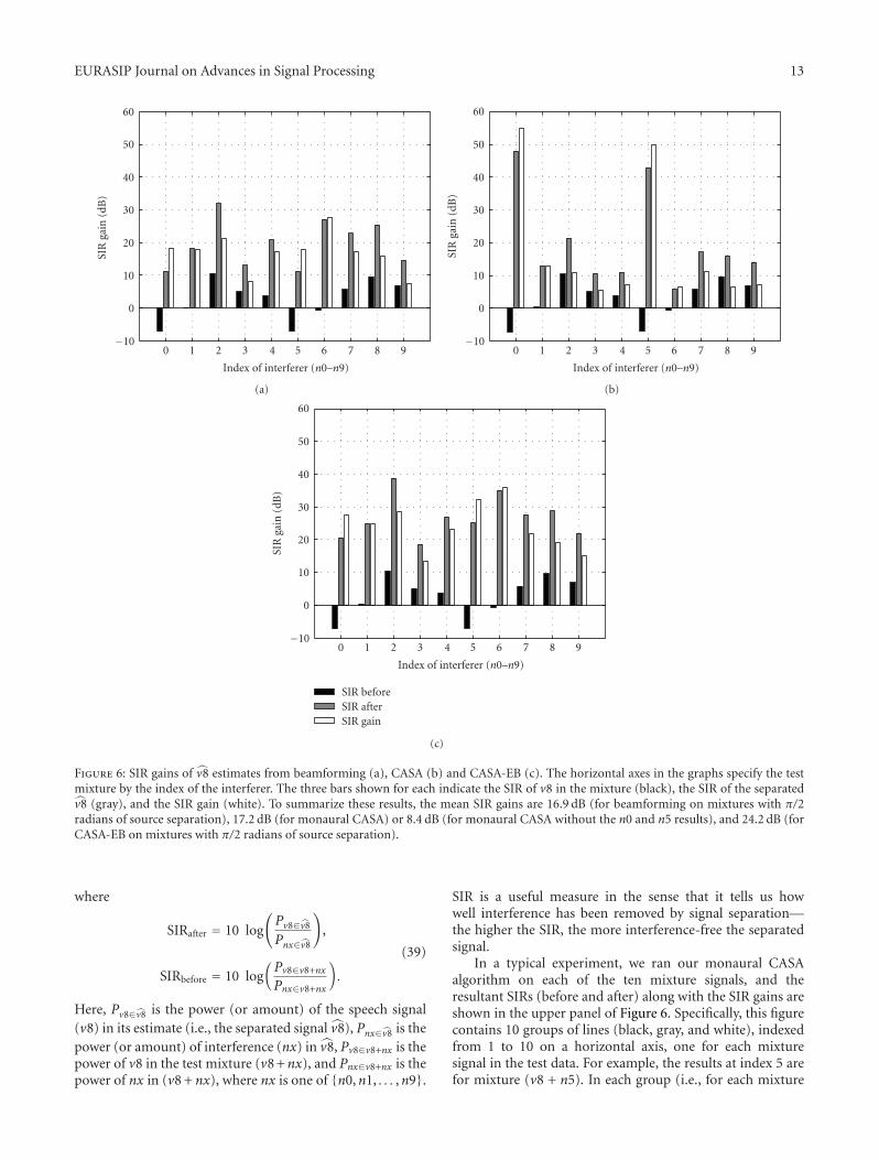
Figure 6: SIR gains of v̂8 estimates from beamforming (a), CASA (b) and CASA-EB (c). The horizontal axes in the graphs specify the testmixture by the index of the interferer. The three bars shown for each indicate the SIR of v8 in the mixture (black), the SIR of the separatedv̂8 (gray), and the SIR gain (white). To summarize these results, the mean SIR gains are 16.9 dB (for beamforming on mixtures with π/2radians of source separation), 17.2 dB (for monaural CASA) or 8.4 dB (for monaural CASA without the n0 and n5 results), and 24.2 dB (forCASA-EB on mixtures with π/2 radians of source separation).

where

SIRafter = 10 log

(Pv8∈v̂8

Pnx∈v̂8

),

SIRbefore = 10 log(Pv8∈v8+nx

Pnx∈v8+nx

).

(39)

Here, Pv8∈v̂8 is the power (or amount) of the speech signal(v8) in its estimate (i.e., the separated signal v̂8), Pnx∈v̂8 is thepower (or amount) of interference (nx) in v̂8, Pv8∈v8+nx is thepower of v8 in the test mixture (v8 +nx), and Pnx∈v8+nx is thepower of nx in (v8 + nx), where nx is one of {n0,n1, . . . ,n9}.

SIR is a useful measure in the sense that it tells us howwell interference has been removed by signal separation—the higher the SIR, the more interference-free the separatedsignal.

In a typical experiment, we ran our monaural CASAalgorithm on each of the ten mixture signals, and theresultant SIRs (before and after) along with the SIR gains areshown in the upper panel of Figure 6. Specifically, this figurecontains 10 groups of lines (black, gray, and white), indexedfrom 1 to 10 on a horizontal axis, one for each mixturesignal in the test data. For example, the results at index 5 arefor mixture (v8 + n5). In each group (i.e., for each mixture


Table 2: Voiced speech signal v8 and the interference signals (n0–n9) from Cooke’s 100 mixtures [8].

ID Description Characterization

v8 Why were you all weary?

n0 1 kHz tone Narrowband, continuous, structured

n1 White noise Wideband, continuous, unstructured

n2 Series of brief noise bursts Wideband, interrupted, unstructured

n3 Teaching laboratory noise Wideband, continuous, partly structured

n4 New wave music Wideband, continuous, structured

n5 FM signal (siren) Locally narrowband, continuous, structured

n6 Telephone ring Wideband, interrupted, structured

n7 Female TIMIT utterance Wideband, continuous, structured

n8 Male TIMIT utterance Wideband, continuous, structured

n9 Female utterance Wideband, continuous, structured

−10

0

10

20

30

40

50

60

70

SIR

gain

(dB

)

0 1 2 3 4 5 6 7 8 9

Interferer (n0–n9)

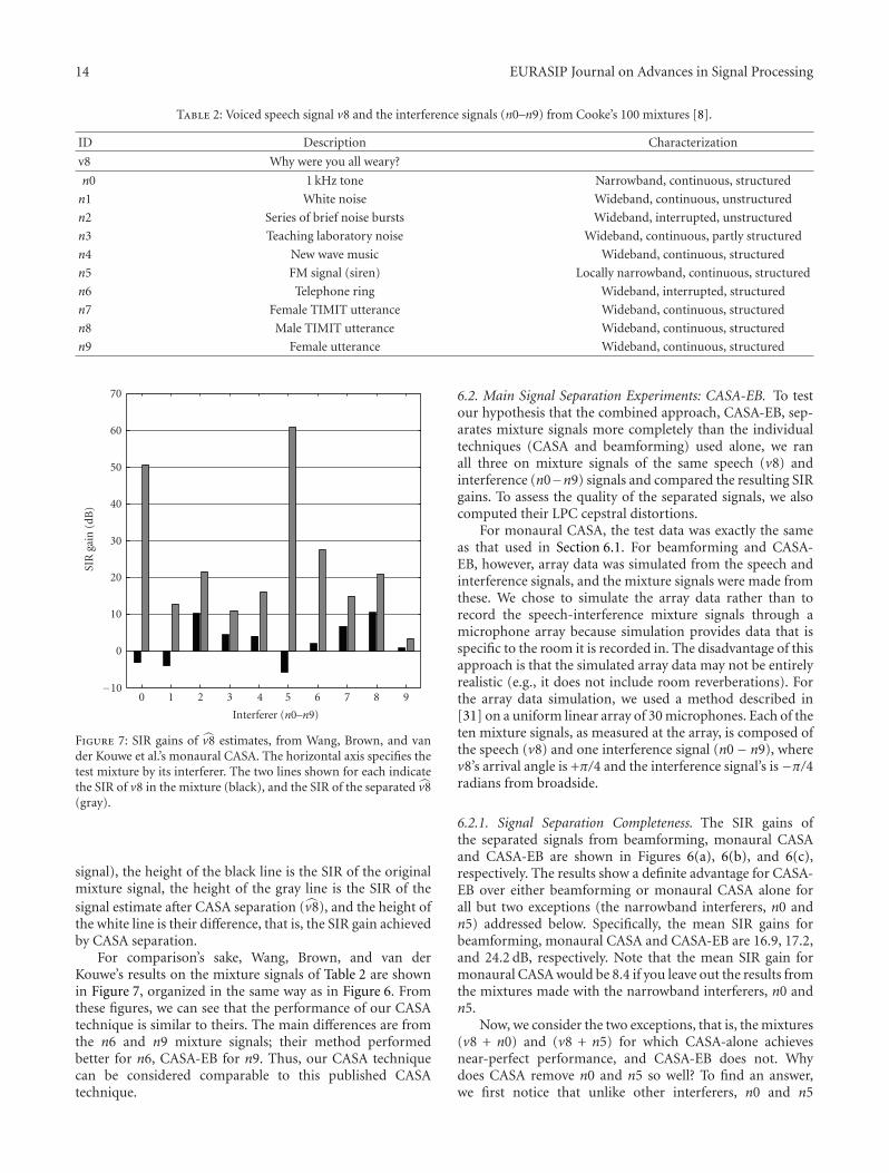
Figure 7: SIR gains of v̂8 estimates, from Wang, Brown, and vander Kouwe et al.’s monaural CASA. The horizontal axis specifies thetest mixture by its interferer. The two lines shown for each indicatethe SIR of v8 in the mixture (black), and the SIR of the separated v̂8(gray).

signal), the height of the black line is the SIR of the originalmixture signal, the height of the gray line is the SIR of thesignal estimate after CASA separation (v̂8), and the height ofthe white line is their difference, that is, the SIR gain achievedby CASA separation.

For comparison’s sake, Wang, Brown, and van derKouwe’s results on the mixture signals of Table 2 are shownin Figure 7, organized in the same way as in Figure 6. Fromthese figures, we can see that the performance of our CASAtechnique is similar to theirs. The main differences are fromthe n6 and n9 mixture signals; their method performedbetter for n6, CASA-EB for n9. Thus, our CASA techniquecan be considered comparable to this published CASAtechnique.

6.2. Main Signal Separation Experiments: CASA-EB. To testour hypothesis that the combined approach, CASA-EB, sep-arates mixture signals more completely than the individualtechniques (CASA and beamforming) used alone, we ranall three on mixture signals of the same speech (v8) andinterference (n0−n9) signals and compared the resulting SIRgains. To assess the quality of the separated signals, we alsocomputed their LPC cepstral distortions.

For monaural CASA, the test data was exactly the sameas that used in Section 6.1. For beamforming and CASA-EB, however, array data was simulated from the speech andinterference signals, and the mixture signals were made fromthese. We chose to simulate the array data rather than torecord the speech-interference mixture signals through amicrophone array because simulation provides data that isspecific to the room it is recorded in. The disadvantage of thisapproach is that the simulated array data may not be entirelyrealistic (e.g., it does not include room reverberations). Forthe array data simulation, we used a method described in[31] on a uniform linear array of 30 microphones. Each of theten mixture signals, as measured at the array, is composed ofthe speech (v8) and one interference signal (n0− n9), wherev8’s arrival angle is +π/4 and the interference signal’s is−π/4radians from broadside.

6.2.1. Signal Separation Completeness. The SIR gains ofthe separated signals from beamforming, monaural CASAand CASA-EB are shown in Figures 6(a), 6(b), and 6(c),respectively. The results show a definite advantage for CASA-EB over either beamforming or monaural CASA alone forall but two exceptions (the narrowband interferers, n0 andn5) addressed below. Specifically, the mean SIR gains forbeamforming, monaural CASA and CASA-EB are 16.9, 17.2,and 24.2 dB, respectively. Note that the mean SIR gain formonaural CASA would be 8.4 if you leave out the results fromthe mixtures made with the narrowband interferers, n0 andn5.

Now, we consider the two exceptions, that is, the mixtures(v8 + n0) and (v8 + n5) for which CASA-alone achievesnear-perfect performance, and CASA-EB does not. Whydoes CASA remove n0 and n5 so well? To find an answer,we first notice that unlike other interferers, n0 and n5


0

1

2

3

4

5

LPC

ceps

tral

dist

orti

on

0 2 4 6 8 10


(a)

0

1

2

3

4

5

LPC

ceps

tral

dist

orti

on

0 2 4 6 8 10


(b)

0

1

2

3

4

5

LPC

ceps

tral

dist

orti

on

0 2 4 6 8 10


(c)

Figure 8: LPC cepstral distortions of v̂8 estimates from beam-forming (a), CASA (b), and CASA-EB (c). As in Figures 6 and 7,the horizontal axes in the graphs specify the test mixture by theindex of the interferer. The value plotted is the mean LPC cepstraldistortion over the duration of the input mixture, v8 + nx, nx ∈{n0,n1, . . . ,n9}; the error bars show the standard deviations.

are narrowband and, in any short period of time, eachhas its power concentrated in a single frequency or a verynarrow frequency band. Now, recall that our CASA approachseparates a signal from interference by grouping harmonicsignal components of a common fundamental, and rejectingother signal components. It does this by first passing thesignal-interference mixture through a filter bank (the hω[n]defined in Section 3), that is, decomposing it into a set ofsubband signals. Then, the autocorrelation for each subbandis computed, forming an autocorrelogram (see Figure 4(b)),and a harmonic group (a fundamental frequency andits overtones) is identified (as described in Section 4.2).After such harmonics are identified, the remaining signalcomponents (interferers) are rejected.

When an interferer is narrowband (such as n0 and n5), itis almost certain that it will be contained entirely in a singlesubband. Furthermore, if the interferer has a lot of power (asin v8 +n0 and v8 +n5), it is going to affect the location of theautocorrelogram peak for that subband. Either the peak inthe subband will correspond to the period of the interferer, ifit is strong relative to the other signal content in the subband,or the peak will at least be pulled towards the interferer.When we use CASA, this will cause the subband to be rejectedfrom the signal estimate, and as a result the interferer willbe completely rejected. This is why CASA works so well inrejecting narrowband interferers.

When CASA-EB is used, the CASA operation is pre-ceeded by spatial filtering (beamforming). When the inter-ferer and the signal come from different directions (as isthe case in v8 + n0 and v8 + n5), this has the affect ofreducing the power of the interferer in the subband that itis in. As a result, the autocorrelogram peak in that subbandwill be much less affected by the interferer compared to theCASA alone case, and as a result, the subband may not berejected in the signal reconstruction, leading to a smaller SIRimprovement than when CASA is used alone. However, wewould like to point out that CASA-EB’s performance in thiscase (on mixtures with narrowband interferers), althoughnot as good as CASA-alone’s dramatic performance, is stillquite decent thanks to the spatial filtering that reduced theinterferers’ power.

6.2.2. Perceptual Quality of Separated Signals. The meanLPC cepstral distortions of the separated signals (v̂8) frombeamforming, monaural CASA, and CASA-EB are shown inFigures 8(a), 8(b), and 8(c), respectively. Here, LPC cepstraldistortion is computed as:

d[r] =

√√√√√1

F + 1·

F∑

f=0

(ln(Pv8[f])− ln

(Pv̂8

[f]))2

, (40)

where r = n/Td is the time index, Td = 160 is the lengthof signal used to compute d[r], Pv8[ f ] is the LPC powerspectral component of v8 at frequency f (computed by theYule-Walker method), and F = 60 corresponds to frequencyfs/2.

The results show that beamforming produces low dis-tortion (1.24 dB averaged over the duration of the separated


signal v̂8 and over all 10 test mixtures), CASA intro-duces somewhat higher distortion (2.17 dB), and CASA-EB is similar to monaural CASA (1.98 dB). The fact thatbeamforming produces lower distortion than CASA maybe because distortion in beamforming comes primarilyfrom incomplete removal of interferers and noise, whilein CASA, additional distortion comes from the removalof target signal components when the target signal hasfrequency content in bands that are dominated by inter-ferer(s). Thus, beamforming generally passes the entiretarget signal with some residual interference (generating lowdistortion), while CASA produces signal estimates that canalso be missing pieces of the target signal (producing moredistortion).

6.2.3. Summary. In summary, CASA-EB separates mixturesignals more completely than either individual method aloneand produces separated signals with rather low spectraldistortion (∼2 dB LPC cepstral distortion). Lower spectraldistortion can be had by using beamforming alone, however,beamforming generally provides less signal separation thanCASA-EB and cannot separate signals from close arrivalangles.

7. Conclusion

In this paper, we proposed a novel approach to acousticsignal separation. Compared to most previously proposedapproaches which use either location or source attributesalone, this approach, called CASA-EB, exploits both locationand source attributes by combining beamforming andauditory scene analysis. Another novel aspect of our work isin the signal component grouping step, which uses clusteringand Kalman filtering to group signal components over timeand frequency.

Experimental results have demonstrated the efficacy ofour proposed approach; overall, CASA-EB provides bettersignal separation performance than beamforming or CASAalone, and while the quality of the separated signals sufferssome degradation, their spectral distortions are rather low(∼2 dB LPC cepstral distortion). Although beyond thescope of this current work, to demonstrate the advantageof combining location and source attributes for acousticsignal separation, further performance improvements maybe achieved by tuning CASA-EB’s parts. For example, usinga higher resolution beamformer may allow CASA-EB to pro-duce separated signals with lower residual interference fromneigboring arrival angles, and using a larger set of sourceattributes could improve performance for harmonic targetsignals and accommodate target signals with nonharmonicstructures.

References

[1] A. J. W. van der Kouwe, D. Wang, and G. J. Brown, “Acomparison of auditory and blind separation techniques forspeech segregation,” IEEE Transactions on Speech and AudioProcessing, vol. 9, no. 3, pp. 189–195, 2001.

[2] P. N. Denbigh and J. Zhao, “Pitch extraction and separation ofoverlapping speech,” Speech Communication, vol. 11, no. 2-3,pp. 119–125, 1992.

[3] T. Nakatani and H. G. Okuno, “Harmonic sound streamsegregation using localization and its application to speechstream segregation,” Speech Communication, vol. 27, no. 3, pp.209–222, 1999.

[4] N. Roman, D. Wang, and G. J. Brown, “Speech segregationbased on sound localization,” The Journal of the AcousticalSociety of America, vol. 114, no. 4, pp. 2236–2252, 2003.

[5] M. Brandstein and D. Ward, Eds., Microphone Arrays,Springer, New York, NY, USA, 2001.

[6] L. Drake, A. K. Katsaggelos, J. C. Rutledge, and J. Zhang,“Sound source separation via computational auditory sceneanalysis-enhanced beamforming,” in Proceedings of the 2ndIEEE Sensor Array and Multichannel Signal Processing Work-shop, Rosslyn, Va, USA, August 2002.

[7] M. Cooke and D. P. W. Ellis, “The auditory organizationof speech and other sources in listeners and computationalmodels,” Speech Communication, vol. 35, no. 3-4, pp. 141–177,2001.

[8] M. Cooke, Modelling auditory processing and organisation,Ph.D. dissertation, The University of Sheffield, Sheffield, UK,1991.

[9] G. Brown, Computational auditory scene analysis: a repre-sentational approach, Ph.D. dissertation, The University ofSheffield, Sheffield, UK, 1992.

[10] D. P. W. Ellis, Prediction-driven computational auditory sceneanalysis, Ph.D. dissertation, MIT, Cambridge, Mass, USA,April 1996.

[11] D. L. Wang and G. J. Brown, “Separation of speech frominterfering sounds based on oscillatory correlation,” IEEETransactions on Neural Networks, vol. 10, no. 3, pp. 684–697,1999.

[12] G. Hu and D. L. Wang, “Monaural speech segregationbased on pitch tracking and amplitude modulation,” IEEETransactions on Neural Networks, vol. 15, no. 5, pp. 1135–1150,2004.

[13] S. N. Wrigley and G. J. Brown, “Recurrent timing neuralnetworks for joint F0-localisation based speech separation,” inProceedings of the IEEE International Conference on Acoustics,Speech, and Signal Processing (ICASSP ’07), vol. 1, pp. 157–160,Honolulu, Hawaii, USA, April 2007.

[14] J. Krolik, “Focused wide-band array processing for spatialspectral estimation,” in Advances in Spectrum Analysis andArray Processing, S. Haykin, Ed., vol. 2 of Prentice Hall SignalProcessing Series and Prentice Hall Advanced Reference Series,chapter 6, pp. 221–261, Prentice-Hall, Englewood-Cliffs, NJ,USA, 1991.

[15] J. Capon, “High-resolution frequency-wavenumber spectrumanalysis,” Proceedings of the IEEE, vol. 57, no. 8, pp. 1408–1418,1969.

[16] D. N. Swingler and J. Krolik, “Source location bias in thecoherently focused high-resolution broad-band beamformer,”IEEE Transactions on Acoustics, Speech, and Signal Processing,vol. 37, no. 1, pp. 143–145, 1989.

[17] M. Wax and T. Kailath, “Detection of signals by informationtheoretic criteria,” IEEE Transactions on Acoustics, Speech, andSignal Processing, vol. 33, no. 2, pp. 387–392, 1985.

[18] H. Akaike, “Information theory and an extension of themaximum likelihood principle,” in Proceedings of the 2ndInternational Symposium on Information Theory, pp. 267–281,1973.


[19] H. Akaike, “A new look at the statistical model identification,”IEEE Transactions on Automatic Control, vol. 19, no. 6, pp.716–723, 1974.

[20] G. Schwartz, “Estimating the dimension of a model,” Annals ofStatistics, vol. 6, pp. 461–464, 1978.

[21] J. Rissanen, “Modeling by shortest data description,” Automat-ica, vol. 14, no. 5, pp. 465–471, 1978.

[22] T. W. Parsons, “Separation of speech from interfering speechby means of harmonic selection,” The Journal of the AcousticalSociety of America, vol. 60, no. 4, pp. 911–918, 1976.

[23] U. Baumann, “Pitch and onset as cues for segregationof musical voices,” in Proceedings of the 2nd InternationalConference on Music Perception and Cognition, February 1992.

[24] G. Brown and M. Cooke, “Perceptual grouping of musicalsounds: a computational model,” The Journal of New MusicResearch, vol. 23, no. 2, pp. 107–132, 1994.

[25] Y. Gu, “A robust pseudo perceptual pitch estimator,” inProceedings of the 2nd European Conference on Speech Com-munication and Technology (EUROSPEECH ’91), pp. 453–456,1991.

[26] M. Weintraub, A theory and computational model of auditorysound separation, Ph.D. dissertation, Stanford University,Stanford, UK, 1985.

[27] R. Gardner, “An algorithm for separating simultaneous vow-els,” British Journal of Audiology, vol. 23, pp. 170–171, 1989.

[28] M. Slaney and R. F. Lyon, “A perceptual pitch detector,” inProceedings of the IEEE International Conference on Acoustics,Speech, and Signal Processing (ICASSP ’90), vol. 1, pp. 357–360,¿Albuquerque, NM, USA, April 1990.

[29] P. F. Assmann and Q. Summerfield, “Modeling the perceptionof concurrent vowels: vowels with different fundamentalfrequencies,” The Journal of the Acoustical Society of America,vol. 88, no. 2, pp. 680–697, 1990.

[30] R. Meddis and M. J. Hewitt, “Virtual pitch and phasesensitivity of a computer model of the auditory periphery—I: pitch identification,” The Journal of the Acoustical Society ofAmerica, vol. 89, no. 6, pp. 2866–2882, 1991.

[31] L. Drake, Sound source separation via computational auditoryscene analysis (casa)-enhanced beamforming, Ph.D. disserta-tion, Northwestern University, December 2001.

[32] U. Baumann, “A procedure for identification and segre-gation of multiple auditory objects,” in Proceedings of theNATO Advanced Study Institute on Computational Hearing, S.Greenberg and M. Slaney, Eds., pp. 211–215, InternationalComputer Science Institute, Berkeley, Calif, USA, 1998.

[33] Y. Bar-Shalom and T. E. Fortmann, Tracking and Data Asso-ciation, vol. 179 of Mathematics in Science and Engineering,Academic Press, New York, NY, USA, 1988.

[34] F. Burgeois and J. C. Lassalle, “Extension of the Munkres algo-rithm for the assignment problems to rectangular matrices,”Communications of the ACM, vol. 14, no. 12, pp. 802–804,1971.

[35] S. S. Blackman, Multiple-Target Tracking with Radar Applica-tions, Artech House, Boston, Mass, USA, 1986.

[36] J. T. Tou and R. C. Gonzalez, Pattern Recognition Principles,Addison-Wesley, Reading, Mass, USA, 1974.

[37] L. Kaufman and P. J. Rousseeuw, Finding Groups in Data: AnIntroduction to Cluster Analysis, John Wiley & Sons, New York,NY, USA, 1990.

[38] S. Theodoridis and K. Koutroumbas, Pattern Recognition,Academic Press, New York, NY, USA, 1999.

[39] B. D. Ripley and N. Hjort, Pattern Recognition and NeuralNetworks, Cambridge University Press, Cambridge, UK, 1995.

[40] R. O. Duda, P. E. Hart, and D. G. Stork, Pattern Classification,John Wiley & Sons, New York, NY, USA, 2nd edition, 2001.

[41] R. Ihaka and R. Gentleman, “R: a language for data analysisand graphics,” Journal of Computational and Graphical Statis-tics, vol. 5, no. 3, pp. 299–314, 1996.

[42] R. Gentleman, R. Ihaka, and R Core Team, “R version 0.63.1,”December 1998, a statistical computation and graphics sys-tem. Re-implementation of the S language, using Schemesemantics, http://www.stat.auckland.ac.nz/r/r.html.

[43] R. A. Becker, J. M. Chambers, and A. R. Wilks, The New SLanguage, Chapman & Hall, London, UK, 1988.

[44] J. M. Chambers and T. J. Hastie, Statistical Models in S,Chapman & Hall, London, UK, 1992.

Documents

A Computational Auditory Scene Analysis-Enhanced Beamforming Approach for Sound Source Separation