HAL Id: hal-01580121https://hal.archives-ouvertes.fr/hal-01580121

Submitted on 1 Sep 2017

HAL is a multi-disciplinary open accessarchive for the deposit and dissemination of sci-entific research documents, whether they are pub-lished or not. The documents may come fromteaching and research institutions in France orabroad, or from public or private research centers.

L’archive ouverte pluridisciplinaire HAL, estdestinée au dépôt et à la diffusion de documentsscientifiques de niveau recherche, publiés ou non,émanant des établissements d’enseignement et derecherche français ou étrangers, des laboratoirespublics ou privés.

A CAP for graphic scores Graphic notation andperformance

Benny Sluchin, Mikhail Malt

To cite this version:Benny Sluchin, Mikhail Malt. A CAP for graphic scores Graphic notation and performance. Tenor2017 - International Conference on Technologies for Music Notation and Representation, May 2017,La Coruña, Spain. �hal-01580121�

A CAP for graphic scores Graphic notation and performance

Benny Sluchin

EIC-Ircam sluchin@ircam.fr

Mikhail Malt Ircam

Mikhail.Malt@ircam.fr

ABSTRACT

Many graphic scores use the pitch versus time presentation, as a natural extension of the usual notation. In the general case, it displays discrete pitches, in a fixed timeline. Nevertheless, graphic scores use a lot of continuous lines, and the vertical dimension can be adapted to a particular performance. In such a way, the instrumentation is free, and the actual range of a particular instrument can be adapted according to the notation. The present article is initiated by a search to provide the performer with adequate tools to approach the execution of such works. A computer assisted performance approach helps the player in the preparation process for both: the time and the pitch approximations. The simulation can enhance the performance in approaching the graphical notation.

.

1. INTRODUCTION The starting point of the present research was a performance issue; works of the 20th century, aimed at concerts and recordings, were approached seriously. The player searched for tools that will help him attain the composer’s intentions as proposed by the printed (graphical) scores. Curiously enough, such tools did not exist, and the precision of the performance was quite lacking. Our work focuses on this category of works and a CAP (Computer Assisted Performance) approach, that is in fact help in preparing the works for performance, in the same way a metronome is.

2. PREVIOUS WORK Since several years now, works having a generic presentation, that is to say, open form, has occupied us. Three examples were discussed: Domaines (1968) by Pierre Boulez, Duel (1959) and Strategy (1962) and Linaia Agon by Iannis Xenakis and Concert for Piano and Orchestra (1958) by John Cage ([1], [2], [3]). Other works by Cage, part of his late “number pieces” were

also accessed [4]. In all these cases, a computer interface that assist the performer in preparing and performing the works were developed. The two main compositions we discuss here, present performance notation difficulties. Conversely to previous work [5]1, our aim is to develop solutions, in a computer-assisted performance study, for trombone version, and offer aural guides to attain a performance, as close as possible to the graphical notations used.

3. TWO EXAMPLES, TWO PROBLEMS

3.1 Alvin Lucier’s Panorama (1993)

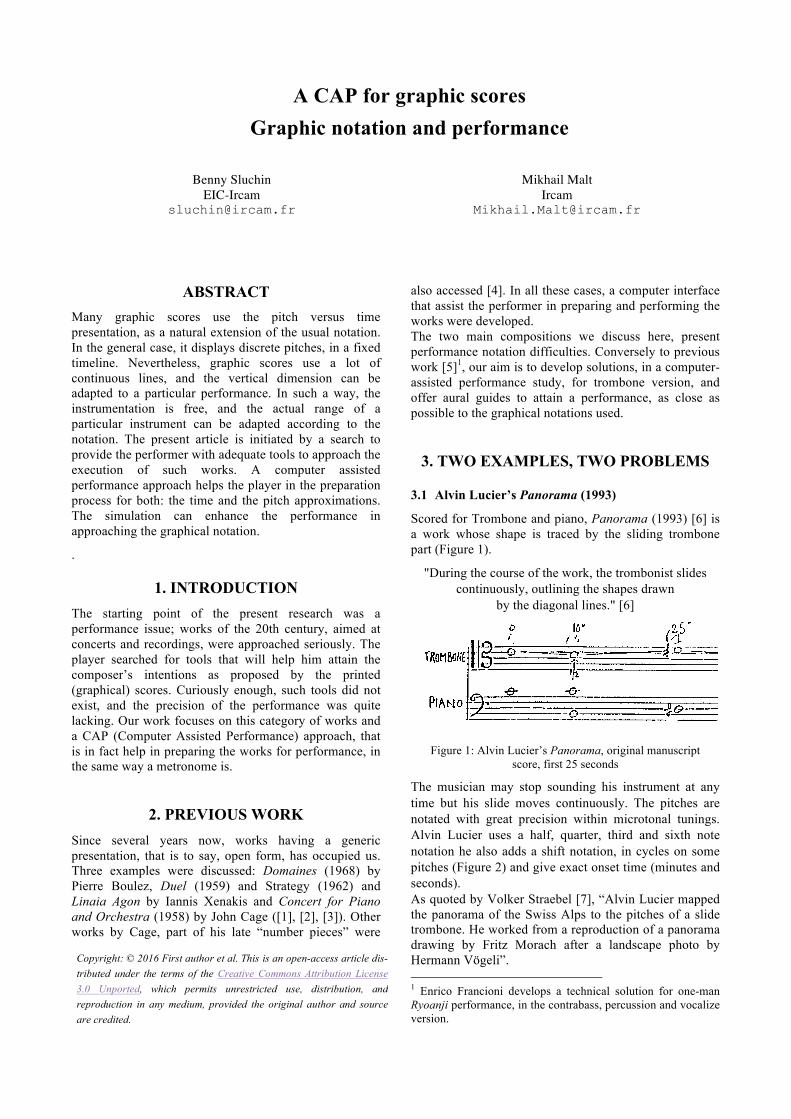
Scored for Trombone and piano, Panorama (1993) [6] is a work whose shape is traced by the sliding trombone part (Figure 1).

"During the course of the work, the trombonist slides continuously, outlining the shapes drawn

by the diagonal lines." [6]

Figure 1: Alvin Lucier’s Panorama, original manuscript

score, first 25 seconds

The musician may stop sounding his instrument at any time but his slide moves continuously. The pitches are notated with great precision within microtonal tunings. Alvin Lucier uses a half, quarter, third and sixth note notation he also adds a shift notation, in cycles on some pitches (Figure 2) and give exact onset time (minutes and seconds). As quoted by Volker Straebel [7], “Alvin Lucier mapped the panorama of the Swiss Alps to the pitches of a slide trombone. He worked from a reproduction of a panorama drawing by Fritz Morach after a landscape photo by Hermann Vögeli”. 1 Enrico Francioni develops a technical solution for one-man Ryoanji performance, in the contrabass, percussion and vocalize version.

Copyright: © 2016 First author et al. This is an open-access article dis- tributed under the terms of the Creative Commons Attribution License 3.0 Unported, which permits unrestricted use, distribution, and reproduction in any medium, provided the original author and source are credited.

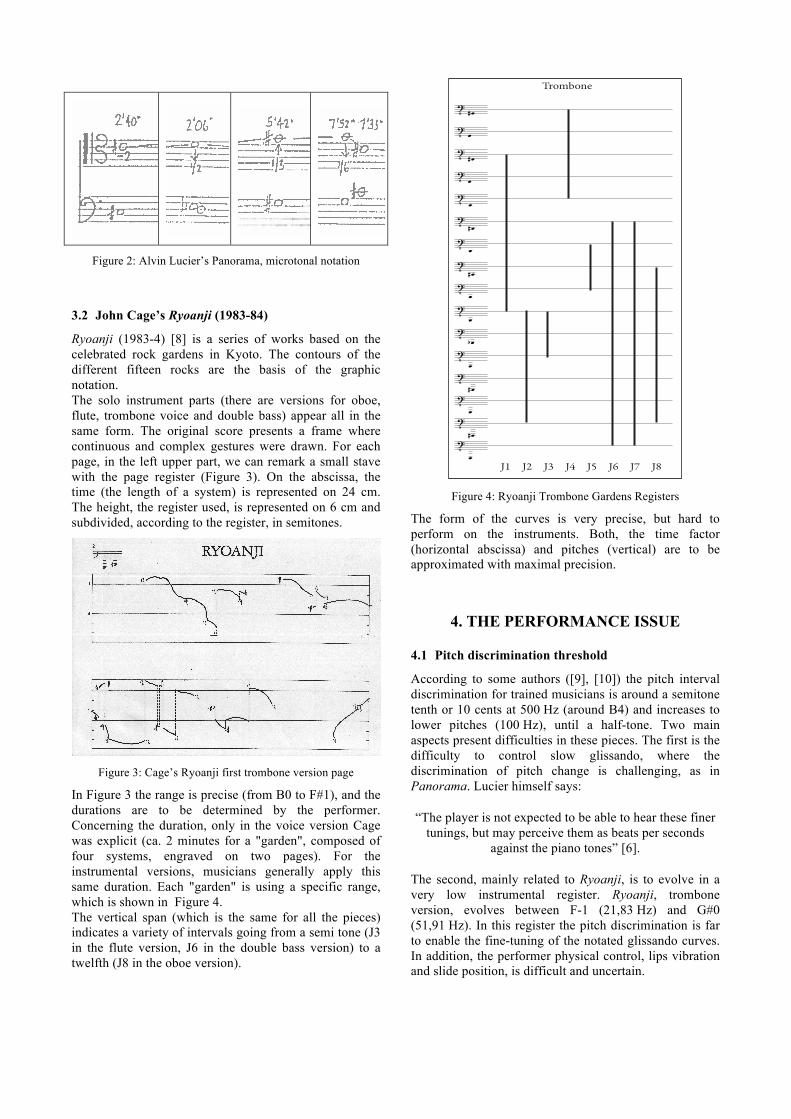
Figure 2: Alvin Lucier’s Panorama, microtonal notation

3.2 John Cage’s Ryoanji (1983-84)

Ryoanji (1983-4) [8] is a series of works based on the celebrated rock gardens in Kyoto. The contours of the different fifteen rocks are the basis of the graphic notation. The solo instrument parts (there are versions for oboe, flute, trombone voice and double bass) appear all in the same form. The original score presents a frame where continuous and complex gestures were drawn. For each page, in the left upper part, we can remark a small stave with the page register (Figure 3). On the abscissa, the time (the length of a system) is represented on 24 cm. The height, the register used, is represented on 6 cm and subdivided, according to the register, in semitones.

Figure 3: Cage’s Ryoanji first trombone version page

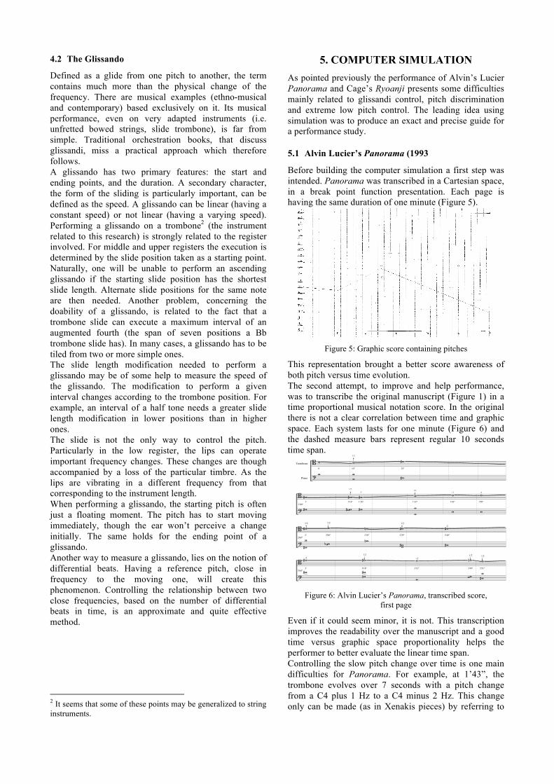
In Figure 3 the range is precise (from B0 to F#1), and the durations are to be determined by the performer. Concerning the duration, only in the voice version Cage was explicit (ca. 2 minutes for a "garden", composed of four systems, engraved on two pages). For the instrumental versions, musicians generally apply this same duration. Each "garden" is using a specific range, which is shown in Figure 4. The vertical span (which is the same for all the pieces) indicates a variety of intervals going from a semi tone (J3 in the flute version, J6 in the double bass version) to a twelfth (J8 in the oboe version).

Figure 4: Ryoanji Trombone Gardens Registers

The form of the curves is very precise, but hard to perform on the instruments. Both, the time factor (horizontal abscissa) and pitches (vertical) are to be approximated with maximal precision.

4. THE PERFORMANCE ISSUE

4.1 Pitch discrimination threshold

According to some authors ([9], [10]) the pitch interval discrimination for trained musicians is around a semitone tenth or 10 cents at 500 Hz (around B4) and increases to lower pitches (100 Hz), until a half-tone. Two main aspects present difficulties in these pieces. The first is the difficulty to control slow glissando, where the discrimination of pitch change is challenging, as in Panorama. Lucier himself says: “The player is not expected to be able to hear these finer

tunings, but may perceive them as beats per seconds against the piano tones” [6].

The second, mainly related to Ryoanji, is to evolve in a very low instrumental register. Ryoanji, trombone version, evolves between F-1 (21,83 Hz) and G#0 (51,91 Hz). In this register the pitch discrimination is far to enable the fine-tuning of the notated glissando curves. In addition, the performer physical control, lips vibration and slide position, is difficult and uncertain.

t œ#t œt œ#t œt œt œ#t œt

œ#t

œt

œt

œbt

œtœ#t

œtœ#t

œt

©

J1 J2 J3 J4 J5 J6 J7 J8

Trombone

4.2 The Glissando

Defined as a glide from one pitch to another, the term contains much more than the physical change of the frequency. There are musical examples (ethno-musical and contemporary) based exclusively on it. Its musical performance, even on very adapted instruments (i.e. unfretted bowed strings, slide trombone), is far from simple. Traditional orchestration books, that discuss glissandi, miss a practical approach which therefore follows. A glissando has two primary features: the start and ending points, and the duration. A secondary character, the form of the sliding is particularly important, can be defined as the speed. A glissando can be linear (having a constant speed) or not linear (having a varying speed). Performing a glissando on a trombone2 (the instrument related to this research) is strongly related to the register involved. For middle and upper registers the execution is determined by the slide position taken as a starting point. Naturally, one will be unable to perform an ascending glissando if the starting slide position has the shortest slide length. Alternate slide positions for the same note are then needed. Another problem, concerning the doability of a glissando, is related to the fact that a trombone slide can execute a maximum interval of an augmented fourth (the span of seven positions a Bb trombone slide has). In many cases, a glissando has to be tiled from two or more simple ones. The slide length modification needed to perform a glissando may be of some help to measure the speed of the glissando. The modification to perform a given interval changes according to the trombone position. For example, an interval of a half tone needs a greater slide length modification in lower positions than in higher ones. The slide is not the only way to control the pitch. Particularly in the low register, the lips can operate important frequency changes. These changes are though accompanied by a loss of the particular timbre. As the lips are vibrating in a different frequency from that corresponding to the instrument length. When performing a glissando, the starting pitch is often just a floating moment. The pitch has to start moving immediately, though the ear won’t perceive a change initially. The same holds for the ending point of a glissando. Another way to measure a glissando, lies on the notion of differential beats. Having a reference pitch, close in frequency to the moving one, will create this phenomenon. Controlling the relationship between two close frequencies, based on the number of differential beats in time, is an approximate and quite effective method.

2 It seems that some of these points may be generalized to string instruments.

5. COMPUTER SIMULATION As pointed previously the performance of Alvin’s Lucier Panorama and Cage’s Ryoanji presents some difficulties mainly related to glissandi control, pitch discrimination and extreme low pitch control. The leading idea using simulation was to produce an exact and precise guide for a performance study.

5.1 Alvin Lucier’s Panorama (1993

Before building the computer simulation a first step was intended. Panorama was transcribed in a Cartesian space, in a break point function presentation. Each page is having the same duration of one minute (Figure 5).

Figure 5: Graphic score containing pitches

This representation brought a better score awareness of both pitch versus time evolution. The second attempt, to improve and help performance, was to transcribe the original manuscript (Figure 1) in a time proportional musical notation score. In the original there is not a clear correlation between time and graphic space. Each system lasts for one minute (Figure 6) and the dashed measure bars represent regular 10 seconds time span.

Figure 6: Alvin Lucier’s Panorama, transcribed score,

first page

Even if it could seem minor, it is not. This transcription improves the readability over the manuscript and a good time versus graphic space proportionality helps the performer to better evaluate the linear time span. Controlling the slow pitch change over time is one main difficulties for Panorama. For example, at 1’43”, the trombone evolves over 7 seconds with a pitch change from a C4 plus 1 Hz to a C4 minus 2 Hz. This change only can be made (as in Xenakis pieces) by referring to

B?

Trombone

Piano

w0w

w↑10"

1/2

ww

w#25"

w#

B?

w# ↑

1'1'00" w#

w#1'14"

1/2

ww#w#

1'16"

-2

w#w↑

1'32"

1/2

ww

w1'43"

+1

w

w1'50"

-2

w

B?

w# ↑2'

1/2

2'00" ww#

w↓2'06"

1/2

wwb

wn2'18"wn

w#↑2'29"

1/2

ww#

w#2'40"

-2

w#

B?

w#3'

-3

3'00" w#w#↓

3'18"

1/2

wwn#w

3'33"

+2

w

wn↓3'49"

1/2

ww

w↓3'51"

1/2

ww#

PanoramaAlvin Lucier

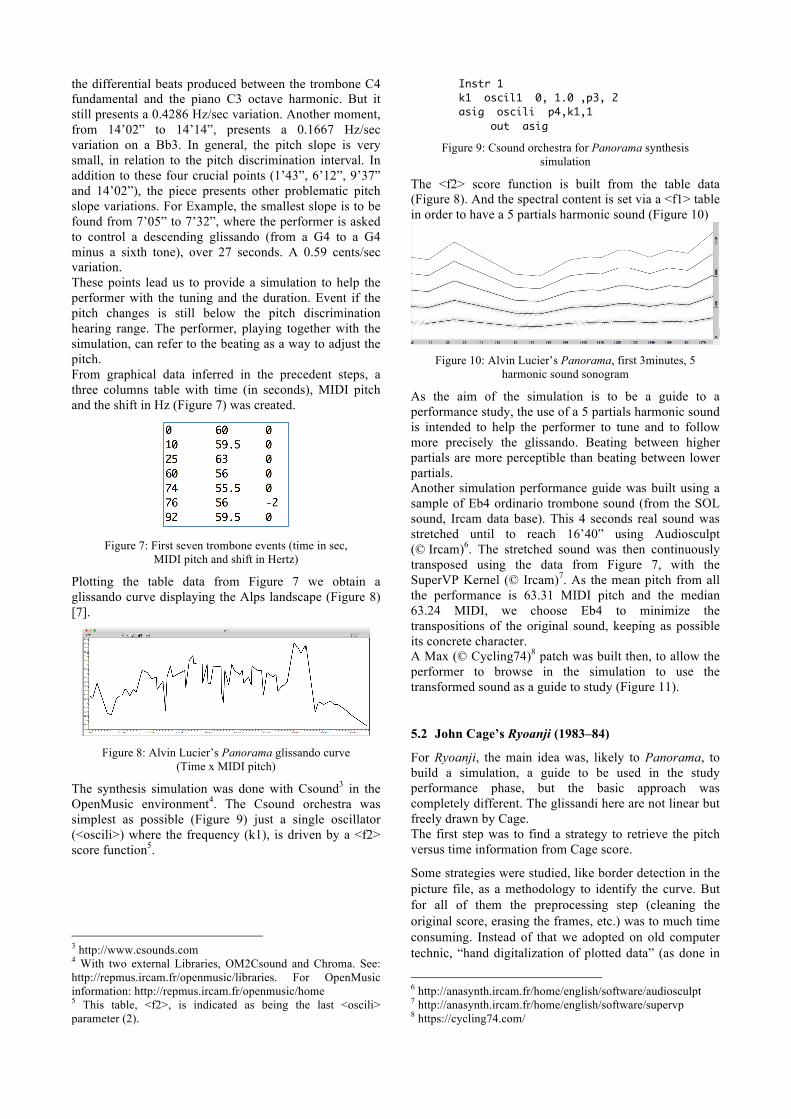
the differential beats produced between the trombone C4 fundamental and the piano C3 octave harmonic. But it still presents a 0.4286 Hz/sec variation. Another moment, from 14’02” to 14’14”, presents a 0.1667 Hz/sec variation on a Bb3. In general, the pitch slope is very small, in relation to the pitch discrimination interval. In addition to these four crucial points (1’43”, 6’12”, 9’37” and 14’02”), the piece presents other problematic pitch slope variations. For Example, the smallest slope is to be found from 7’05” to 7’32”, where the performer is asked to control a descending glissando (from a G4 to a G4 minus a sixth tone), over 27 seconds. A 0.59 cents/sec variation. These points lead us to provide a simulation to help the performer with the tuning and the duration. Event if the pitch changes is still below the pitch discrimination hearing range. The performer, playing together with the simulation, can refer to the beating as a way to adjust the pitch. From graphical data inferred in the precedent steps, a three columns table with time (in seconds), MIDI pitch and the shift in Hz (Figure 7) was created.

Figure 7: First seven trombone events (time in sec,

MIDI pitch and shift in Hertz)

Plotting the table data from Figure 7 we obtain a glissando curve displaying the Alps landscape (Figure 8) [7].

Figure 8: Alvin Lucier’s Panorama glissando curve

(Time x MIDI pitch)

The synthesis simulation was done with Csound3 in the OpenMusic environment4. The Csound orchestra was simplest as possible (Figure 9) just a single oscillator (<oscili>) where the frequency (k1), is driven by a <f2> score function5.

3 http://www.csounds.com 4 With two external Libraries, OM2Csound and Chroma. See: http://repmus.ircam.fr/openmusic/libraries. For OpenMusic information: http://repmus.ircam.fr/openmusic/home 5 This table, <f2>, is indicated as being the last <oscili> parameter (2).

Instr 1 k1 oscil1 0, 1.0 ,p3, 2 asig oscili p4,k1,1 out asig

Figure 9: Csound orchestra for Panorama synthesis simulation

The <f2> score function is built from the table data (Figure 8). And the spectral content is set via a <f1> table in order to have a 5 partials harmonic sound (Figure 10)

Figure 10: Alvin Lucier’s Panorama, first 3minutes, 5

harmonic sound sonogram

As the aim of the simulation is to be a guide to a performance study, the use of a 5 partials harmonic sound is intended to help the performer to tune and to follow more precisely the glissando. Beating between higher partials are more perceptible than beating between lower partials. Another simulation performance guide was built using a sample of Eb4 ordinario trombone sound (from the SOL sound, Ircam data base). This 4 seconds real sound was stretched until to reach 16’40” using Audiosculpt (© Ircam)6. The stretched sound was then continuously transposed using the data from Figure 7, with the SuperVP Kernel (© Ircam)7. As the mean pitch from all the performance is 63.31 MIDI pitch and the median 63.24 MIDI, we choose Eb4 to minimize the transpositions of the original sound, keeping as possible its concrete character. A Max (© Cycling74)8 patch was built then, to allow the performer to browse in the simulation to use the transformed sound as a guide to study (Figure 11).

5.2 John Cage’s Ryoanji (1983–84)

For Ryoanji, the main idea was, likely to Panorama, to build a simulation, a guide to be used in the study performance phase, but the basic approach was completely different. The glissandi here are not linear but freely drawn by Cage. The first step was to find a strategy to retrieve the pitch versus time information from Cage score.

Some strategies were studied, like border detection in the picture file, as a methodology to identify the curve. But for all of them the preprocessing step (cleaning the original score, erasing the frames, etc.) was to much time consuming. Instead of that we adopted on old computer technic, “hand digitalization of plotted data” (as done in

6 http://anasynth.ircam.fr/home/english/software/audiosculpt 7 http://anasynth.ircam.fr/home/english/software/supervp 8 https://cycling74.com/

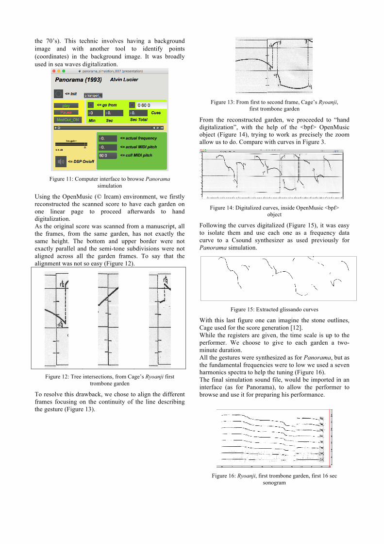
the 70’s). This technic involves having a background image and with another tool to identify points (coordinates) in the background image. It was broadly used in sea waves digitalization.

Figure 11: Computer interface to browse Panorama

simulation

Using the OpenMusic (© Ircam) environment, we firstly reconstructed the scanned score to have each garden on one linear page to proceed afterwards to hand digitalization. As the original score was scanned from a manuscript, all the frames, from the same garden, has not exactly the same height. The bottom and upper border were not exactly parallel and the semi-tone subdivisions were not aligned across all the garden frames. To say that the alignment was not so easy (Figure 12).

Figure 12: Tree intersections, from Cage’s Ryoanji first

trombone garden

To resolve this drawback, we chose to align the different frames focusing on the continuity of the line describing the gesture (Figure 13).

Figure 13: From first to second frame, Cage’s Ryoanji,

first trombone garden

From the reconstructed garden, we proceeded to “hand digitalization”, with the help of the <bpf> OpenMusic object (Figure 14), trying to work as precisely the zoom allow us to do. Compare with curves in Figure 3.

Figure 14: Digitalized curves, inside OpenMusic <bpf>

object

Following the curves digitalized (Figure 15), it was easy to isolate them and use each one as a frequency data curve to a Csound synthesizer as used previously for Panorama simulation.

Figure 15: Extracted glissando curves

With this last figure one can imagine the stone outlines, Cage used for the score generation [12]. While the registers are given, the time scale is up to the performer. We choose to give to each garden a two-minute duration. All the gestures were synthesized as for Panorama, but as the fundamental frequencies were to low we used a seven harmonics spectra to help the tuning (Figure 16). The final simulation sound file, would be imported in an interface (as for Panorama), to allow the performer to browse and use it for preparing his performance.

Figure 16: Ryoanji, first trombone garden, first 16 sec

sonogram

6. CONCLUSIONS The two pieces treated here take advantage of graphical notation but present essential difficulties in performance. We propose here a computer strategy, simulation based, to assist the musician in the preparation and performance. Concerning Panorama, while we found a way to bring a possible assistance for the glissando control and fine-tuning, the optimization for the glissandi position changes still is to do. We look forward to deal with it mainly with a constraint system. Concerning Ryoanji, the main problem (glissando control and fine-tuning) still unsolved. As pointed previously, main parts from this work still impracticable, from cognitive and instrumental reasons. Ryoanji evolves in the extreme lower register what makes very difficult to control and listen to the small microtonal waves. For the first garden (where Cage’s register is from B1 to F#1) the gestures (according with our hand digitalization) evolve between C1 minus 19 cents (32.35 Hz) and a F#1 minus 14 cents (45.88 Hz). We have two pieces mainly based on glissandi, but with two different performance goals. While in Panorama Lucier expects for a precise pitch and time performance, in Ryoanji, the graphical notation has not only a score function, but also an inspirational and poetic purpose. As stated in the Ryoanji instructions: “The glissandi are to be played smoothly and much as is

possible like sound events in nature rather than sounds in music.” [8]

Composers, inspired by extra musical facts or concepts can use sonification as an inspiration way. Translating graphic or visual aspects in musical notation can be source of novelty and challenge, but sometimes it can be source of difficulty. The notation graphic space does not have the same properties as the basic pitch versus time real space. If in the graphic space, we can represent any pitch interval size, it is just a scale question dependence. In hearing world, humans are bounded by their cognitive pitch thresholds. While in the graphic space, we can navigate in the time line, jumping from future to past and vice-versa, in the real world the time appears to be irreversible.

7. REFERENCES [1] B. Sluchin, M. Malt, “Open form and two

combinatorial musical models: The cases of Domaines and Duel”, 3rd International Conference on Mathematics and Computation in Music, Paris, June 15-17, 2011, p. 211-217.

[2] M. Malt, B. Sluchin, “Théorie des jeux et structure formelle dans Duel (1959) et Stratégie (1962) de Xenakis”, L’influence des théories scientifiques sur le renouvellement des formes musicales dans la musique contemporaine, Symposium, organized by

M. Grabócz, CDMC, Paris, 28 november 2014. https://www.youtube.com/watch?v=ZixIYc7iL84&feature=youtube_gdata

[3] B. Sluchin, “Linaia-Agon Towards an Interpretation Based on the Theory”, International Symposium Iannis Xenakis, M. Solomos, A. Georgaki, G. Zervos (Ed.), Athens, May 2005, 1–16. http://Cicm.Mshparisnord.org/ColloqueXenakis/

[4] B. Sluchin, M. Malt, “Interpretation and Computer Assistance in John Cage’s Concert for Piano and Orchestra (1957-58)”, SMC - Sound and Music Computing Conference, 2010, pp. 1 – 8.

[5] E. Francioni, “Csound for Cage's Ryoanji”, Csound Journal, vol. 18, 2014, 1 – 20. http://www.csounds.com/journal/issue18/francioni.html

[6] A. Lucier, Panorama for trombone and piano, manuscript score, 1993.

[7] V. Straebel, “The Sonification Metaphor in Instrumental Music and Sonification’s Romantic Implications”, The 16th International Conference on Auditory Display (ICAD-2010), 2010, pp. 1 – 8.

[8] J. Cage, Ryoanji for Trombone Solo, Henmar Press Inc., 1985.

[9] J. H. McDermott, M. V. Keebler, C. Micheyl, A. J. Oxenham, “Musical intervals and relative pitch: Frequency resolution, not interval resolution, is special” The Journal of the Acoustical Society of America, vol. 128, no 4, 2010, pp. 1943 – 1951.

[10] F. Bianchi, S. Santurette, D. Wendt, T. Dau, “Pitch discrimination in musicians and non-musicians: Effects of harmonic resolvability and processing effort” Journal of the Association for Research in Otolaryngology: JARO, vol. 17, 2016, pp. 69 – 79.

[11] J. Cage, “Ryoanji: Solos for Oboe, Flute, Contrabass, Voice, Trombone with Percussion or Orchestral Obbligato (1983-85)”, PAJ: a Journal of Performance and Art, vol. 31, no 3, 2009, pp. 58 – 64.

[12] M. Fowler, “Finding Cage at Ryōan-ji Through a Re-Modelling of Variations II.” Perspectives of New Music, vol. 47, no 1, Winter, 2009, pp. 174 – 191.

[13] K. Schöning, “Ryoân-ji: oder die Gärten der Leere”, Neue Zeitschrift Für Musik (1991-), vol. 155, no 5, 1994, pp. 24 – 27.