A Boundedness of a Batch Gradient Method with Smoothing L1⁄2 Regularization for Pi-sigma Neural Networks

International Journal of Science and Research (IJSR) ISSN (Online): 2319-7064

Impact Factor (2012): 3.358

Volume 3 Issue 11, November 2014 www.ijsr.net

Licensed Under Creative Commons Attribution CC BY

A Boundedness of a Batch Gradient Method with Smoothing L1 2⁄ Regularization for Pi-sigma Neural

Networks

Kh. Sh. Mohamed1,2, Y. Sh. Mohammed3,4,5, Abd Elmoniem A. Elzain3,6, Mohamed El-Hafiz M. N. 3,7, and Elnoor. A. A. Noh3,8

1 School of Mathematical Sciences, Dalian University of Technology, Dalian 116024, PR China

2 Mathematical Department, College of Science, Dalanj University, Dalanj, Sudan

3 Department of Physics, College of Science & Art, Qassim University, Oklat Al- Skoor, P.O.Box: 111, Saudi Arabia.

4 Physics Department, College of Education, Dalanj University, Dalanj, Sudan

5 Africa City for Technology, Khartoum, Sudan

6 Department of Physics, University of Kassala, Kassala, P.O.Box: 266, Sudan

7 Mathematical Department, College of Education, Zalingy University, Zalingy, Sudan

8 Department of Chemistry, College of Art & Science, Albaha University, Baljurashi, Saudi Arabia.

Abstract: This paper considers a batch gradient method with 𝑳𝑳𝟏𝟏 𝟐𝟐⁄ regularization for Pi –sigma neural networks. In origin, by introducing an 𝑳𝑳𝟏𝟏 𝟐𝟐⁄ regularization term involves absolute value and is not differentiable into the error function. A key point of this paper, specifically, the smoothing 𝑳𝑳𝟏𝟏 𝟐𝟐⁄ regularization is a term proportional to the norm of the weights. The role of the smoothing 𝑳𝑳𝟏𝟏 𝟐𝟐⁄ regularization term is to control the magnitude of the weights and to improve the generalization performance of the networks. The weights are proved to be bounded during the training process, thus the conditions that are required for convergence analysis of batch gradient method in literature are simplified. Keywords: Batch gradient method, Pi-sigma neural network, L½ regularization, Boundedness. 1. Introduction In fact, higher order neural networks (HONN) have been widely applied in many applications such as intention to enhance the nonlinear descriptive capacity of the feed forward multilayer perceptron networks [1 - 6]. Pi-sigma neural network (PSNN) is a class of higher-order feed forward polynomial neural network and is known to provide inherently more powerful mapping abilities than traditional feed forward neural networks. The (PSNN) modules are widely used for pattern classification and approximation problems [7 - 9]. By adding a penalty term of the error function [10 - 16]. The penalty has become a common practice to make the network weights keeping bounded during the training process. The boundedness of the weights is an obvious fact when a convergence training method ‘’ such as the quadratic programming used in support vector machines in [17] is used to minimize the cost function with penalty term. When using online gradient method to minimize the cost of error function with regularization penalty term, the boundedness of weights is not obvious because the decrease of the cost function and convergence of the method during the learning process are usually obtained by first condition the network weights are bounded. Recently, most of the studies have been focused on the L1\2 regularization penalty term adding to the error function usual is not smooth at the origin, which causes difficulty in the

convergence analysis to speed this drawback, we use the modified L1\2 regularization term is proposed by the usual one at the origin [18, 19], in [18] the L1\2 regularization term is introduced into the batch gradient learning algorithm for the pruning of FNN. Some convergence analyses of the online gradient method (OGM for short) with fixed order inputs (OGM_F) and with special stochastic inputs (OGM_SS) for PSNN were respectively presented in [20,21]. Especially, convergence analysis of the online gradient learning algorithm with L1\2 regularization term for the pruning of FNN [19]. However, in [19 - 21] obtain both the weak and strong convergence results. The main purpose of this paper , in doing so, by prove that the weights are indeed bounded deterministically in the batch gradient learning algorithm process by adding a smoothing L1\2 regularization, a term proportional to the norm of the weights. That the weights of the network will keep bounded in the training process. The rest of this paper is organized as follows. The network model and the batch gradient method with smoothing L1\2 regularization are described in the section. The convergence of this algorithm is discussed and a convergence theorem is established in section 3. and conclusion in section 4.

Paper ID: OCT14878 819

http://creativecommons.org/licenses/by/4.0/�

https://www.researchgate.net/publication/243767164_Regularization_Networks_and_Support_Vector_Machines?el=1_x_8&enrichId=rgreq-f3dda16b16be50c407de04444d5bfe63-XXX&enrichSource=Y292ZXJQYWdlOzI2ODI3OTQwNDtBUzoxNjM5ODE2MDM5MDk2MzJAMTQxNjEwNzY2OTg3MQ==

https://www.researchgate.net/publication/259109435_Batch_gradient_method_with_smoothing_L-12_regularization_for_training_of_feedforward_neural_networks?el=1_x_8&enrichId=rgreq-f3dda16b16be50c407de04444d5bfe63-XXX&enrichSource=Y292ZXJQYWdlOzI2ODI3OTQwNDtBUzoxNjM5ODE2MDM5MDk2MzJAMTQxNjEwNzY2OTg3MQ==


https://www.researchgate.net/publication/260213363_Convergence_of_online_gradient_method_for_feedforward_neural_networks_with_smoothing_L12_regularization_penalty?el=1_x_8&enrichId=rgreq-f3dda16b16be50c407de04444d5bfe63-XXX&enrichSource=Y292ZXJQYWdlOzI2ODI3OTQwNDtBUzoxNjM5ODE2MDM5MDk2MzJAMTQxNjEwNzY2OTg3MQ==


https://www.researchgate.net/publication/256504640_Probability_and_Measure?el=1_x_8&enrichId=rgreq-f3dda16b16be50c407de04444d5bfe63-XXX&enrichSource=Y292ZXJQYWdlOzI2ODI3OTQwNDtBUzoxNjM5ODE2MDM5MDk2MzJAMTQxNjEwNzY2OTg3MQ==

https://www.researchgate.net/publication/4253879_Convergence_of_Online_Gradient_Algorithm_with_Stochastic_Inputs_for_Pi-Sigma_Neural_Networks?el=1_x_8&enrichId=rgreq-f3dda16b16be50c407de04444d5bfe63-XXX&enrichSource=Y292ZXJQYWdlOzI2ODI3OTQwNDtBUzoxNjM5ODE2MDM5MDk2MzJAMTQxNjEwNzY2OTg3MQ==






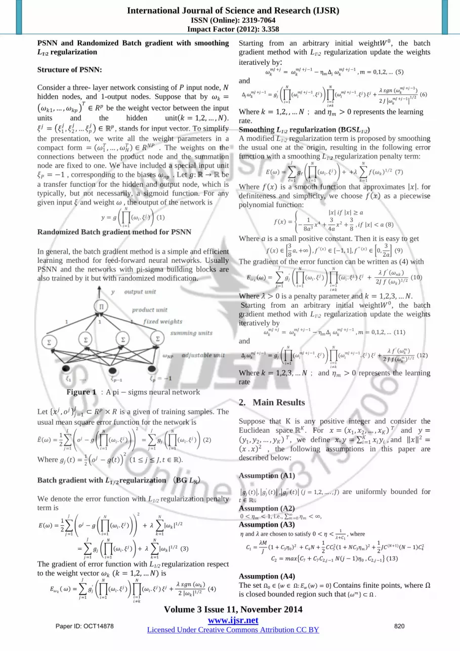
PSNN and Randomized Batch gradient with smoothing L1\2 regularization Structure of PSNN: Consider a three- layer network consisting of 𝑃𝑃 input node, 𝑁𝑁 hidden nodes, and 1-output nodes. Suppose that by 𝜔𝜔𝑘𝑘 =�𝜔𝜔𝑘𝑘1, … ,𝜔𝜔𝑘𝑘𝑘𝑘 �

𝑇𝑇 ∈ 𝑅𝑅𝑘𝑘 be the weight vector between the input units and the hidden unit(𝑘𝑘 = 1,2, … ,𝑁𝑁). 𝜉𝜉𝑗𝑗 = �𝜉𝜉1

𝑗𝑗 , 𝜉𝜉2𝑗𝑗 , … 𝜉𝜉𝑘𝑘

𝑗𝑗 � ∈ ℝ𝑘𝑘 , stands for input vector. To simplify the presentation, we write all the weight parameters in a compact form = (𝜔𝜔1

𝑇𝑇 , … ,𝜔𝜔𝑁𝑁𝑇𝑇 ) ∈ 𝑅𝑅𝑁𝑁𝑃𝑃 . The weights on the

connections between the product node and the summation node are fixed to one. We have included a special input unit 𝜉𝜉𝑃𝑃 = −1 , corresponding to the biases 𝜔𝜔𝑛𝑛𝑘𝑘 . Let 𝑔𝑔:ℝ → ℝ be a transfer function for the hidden and output node, which is typically, but not necessarily, a sigmoid function. For any given input 𝜉𝜉 and weight 𝜔𝜔 , the output of the network is

𝑦𝑦 = 𝑔𝑔 ��(𝜔𝜔𝑖𝑖 . 𝜉𝜉𝑗𝑗 )𝑁𝑁

𝑖𝑖=1

� (1)

Randomized Batch gradient method for PSNN In general, the batch gradient method is a simple and efficient learning method for feed-forward neural networks. Usually PSNN and the networks with pi-sigma building blocks are also trained by it but with randomized modification.

𝐅𝐅𝐅𝐅𝐅𝐅𝐅𝐅𝐅𝐅𝐅𝐅 𝟏𝟏 ：A pi − sigms neural network

Let {𝑥𝑥𝑗𝑗 , 𝑜𝑜𝑗𝑗 }𝑗𝑗=1

𝐽𝐽 ⊂ 𝑅𝑅𝑘𝑘 × 𝑅𝑅 is a given of training samples. The usual mean square error function for the network is

𝐸𝐸�(𝜔𝜔) =12��𝑜𝑜𝑗𝑗 − 𝑔𝑔 ��(𝜔𝜔𝑖𝑖 . 𝜉𝜉𝑗𝑗 )

𝑁𝑁

𝑖𝑖=1

��

2

= �𝑔𝑔𝑗𝑗

𝐽𝐽

𝑗𝑗=1

��(𝜔𝜔𝑖𝑖 . 𝜉𝜉𝑗𝑗 )𝑁𝑁

𝑖𝑖=1

� (2)𝐽𝐽

𝑗𝑗=1

Where 𝑔𝑔𝑗𝑗 (𝑡𝑡) = 12�𝑜𝑜𝑗𝑗 − 𝑔𝑔(𝑡𝑡)�

2 (1 ≤ 𝑗𝑗 ≤ 𝐽𝐽, 𝑡𝑡 ∈ ℝ).

Batch gradient with 𝑳𝑳𝟏𝟏 𝟐𝟐⁄ regularization （BG L½） We denote the error function with L1/2 regularization penalty term is

𝐸𝐸(𝜔𝜔) =12��𝑜𝑜𝑗𝑗 − 𝑔𝑔 ��(𝜔𝜔𝑖𝑖 . 𝜉𝜉𝑗𝑗 )

𝑁𝑁

𝑖𝑖=1

��

2

𝐽𝐽

𝑗𝑗=1

+ 𝜆𝜆 �|𝜔𝜔𝑘𝑘 |1 2⁄𝑁𝑁

𝑘𝑘=1

= �𝑔𝑔𝑗𝑗

𝐽𝐽

𝑗𝑗=1


𝑖𝑖=1

� + 𝜆𝜆 �|𝜔𝜔𝑘𝑘 |1 2⁄𝑁𝑁

𝑘𝑘=1

(3)

The gradient of error function with L1/2 regularization respect to the weight vector 𝜔𝜔𝑘𝑘 (𝑘𝑘 = 1,2, …𝑁𝑁) is

𝐸𝐸𝜔𝜔𝑘𝑘( 𝜔𝜔) = �𝑔𝑔𝑗𝑗′ ��(𝜔𝜔𝑖𝑖 . 𝜉𝜉𝑗𝑗

𝑁𝑁

𝑖𝑖=1

)�𝐽𝐽

𝑗𝑗=1

�(𝜔𝜔𝑖𝑖 . 𝜉𝜉𝑗𝑗 )𝑁𝑁

𝑖𝑖=1𝑖𝑖≠𝑘𝑘

𝜉𝜉𝑗𝑗 + 𝜆𝜆 𝑠𝑠𝑔𝑔𝑛𝑛 (𝜔𝜔𝑘𝑘)

2 |𝜔𝜔𝑘𝑘 |1 2⁄ (4)

Starting from an arbitrary initial weight𝑊𝑊0, the batch gradient method with L1\2 regularization update the weights iteratively by:

𝜔𝜔𝑘𝑘𝑚𝑚𝐽𝐽 +𝑗𝑗 = 𝜔𝜔𝑘𝑘

𝑚𝑚𝐽𝐽 +𝑗𝑗−1 − ηm∆j 𝜔𝜔𝑘𝑘𝑚𝑚𝐽𝐽+𝑗𝑗−1 ,𝑚𝑚 = 0,1,2, … (5)

and

∆𝑗𝑗𝜔𝜔𝑘𝑘𝑚𝑚𝐽𝐽 +𝑗𝑗−1 = 𝑔𝑔𝑗𝑗′ ��(𝜔𝜔𝑖𝑖

𝑚𝑚𝐽𝐽 +𝑗𝑗−1. 𝜉𝜉𝑗𝑗𝑁𝑁

𝑖𝑖=1

)��(𝜔𝜔𝑖𝑖𝑚𝑚𝐽𝐽 +𝑗𝑗−1. 𝜉𝜉𝑗𝑗 )

𝑁𝑁


𝜉𝜉𝑗𝑗 + 𝜆𝜆 𝑠𝑠𝑔𝑔𝑛𝑛 (𝜔𝜔𝑘𝑘

𝑚𝑚𝐽𝐽 +𝑗𝑗−1)

2 𝐽𝐽 �𝜔𝜔𝑘𝑘𝑚𝑚𝐽𝐽 +𝑗𝑗−1�

1 2⁄ (6)

Where 𝑘𝑘 = 1,2, , …𝑁𝑁 ； and 𝜂𝜂𝑚𝑚 > 0 represents the learning rate. Smoothing L1\2 regularization (BGSL1\2) A modified L1\2 regularization term is proposed by smoothing the usual one at the origin, resulting in the following error function with a smoothing L1\2 regularization penalty term:

𝐸𝐸(𝜔𝜔) = �𝑔𝑔ℓ

𝐽𝐽

ℓ=1


𝑖𝑖=1

� + +𝜆𝜆 �𝑓𝑓(𝜔𝜔𝑘𝑘)1 2⁄𝑁𝑁

𝑘𝑘=1

(7)

Where 𝑓𝑓(𝑥𝑥) is a smooth function that approximates |𝑥𝑥|. for definiteness and simplicity, we choose 𝑓𝑓(𝑥𝑥) as a piecewise polynomial function:

𝑓𝑓(𝑥𝑥) = �|𝑥𝑥| 𝑖𝑖𝑓𝑓 |𝑥𝑥| ≥ 𝑎𝑎

−1

8𝑎𝑎3 𝑥𝑥4 +

34𝑎𝑎

𝑥𝑥2 +38

, 𝑖𝑖𝑓𝑓 |𝑥𝑥| < 𝑎𝑎 (8)

�

Where a is a small positive constant. Then it is easy to get 𝑓𝑓(𝑥𝑥) ∈ �

38𝑎𝑎, +∞� ,𝑓𝑓′(𝑥𝑥) ∈ [−1, 1],𝑓𝑓′′ (𝑥𝑥) ∈ �0,

32𝑎𝑎� (9)

The gradient of the error function can be written as (4) with

𝐸𝐸𝜔𝜔𝑘𝑘(𝜔𝜔) = �𝑔𝑔𝑗𝑗′ ��(𝜔𝜔𝑖𝑖 . 𝜉𝜉𝑗𝑗

𝑁𝑁

𝑖𝑖=1

)�𝐽𝐽

𝑗𝑗=1

�(𝜔𝜔𝑖𝑖 . 𝜉𝜉𝑗𝑗 )𝑁𝑁


𝜉𝜉𝑗𝑗 + 𝜆𝜆 𝑓𝑓′(𝜔𝜔𝑛𝑛𝑘𝑘 )

2𝐽𝐽 𝑓𝑓 (𝜔𝜔𝑘𝑘)1 2⁄ (10)

Where 𝜆𝜆 > 0 is a penalty parameter and 𝑘𝑘 = 1,2,3, …𝑁𝑁. Starting from an arbitrary initial weight𝑊𝑊0, the batch gradient method with L1\2 regularization update the weights iteratively by

𝜔𝜔𝑘𝑘𝑚𝑚𝐽𝐽 +𝑗𝑗 = 𝜔𝜔𝑘𝑘

𝑚𝑚𝐽𝐽 +𝑗𝑗−1 − ηm∆j 𝜔𝜔𝑘𝑘𝑚𝑚𝐽𝐽+𝑗𝑗−1 ,𝑚𝑚 = 0,1,2, … (11)

and

∆𝑗𝑗𝜔𝜔𝑘𝑘𝑚𝑚𝐽𝐽 +𝑗𝑗−1 = 𝑔𝑔𝑗𝑗′ ��(𝜔𝜔𝑖𝑖

𝑚𝑚𝐽𝐽 +𝑗𝑗−1. 𝜉𝜉𝑗𝑗𝑁𝑁

𝑖𝑖=1


𝑁𝑁


𝜉𝜉𝑗𝑗 +𝜆𝜆 𝑓𝑓′(𝜔𝜔𝑘𝑘

𝑚𝑚)2 𝐽𝐽 𝑓𝑓(𝜔𝜔𝑘𝑘

𝑚𝑚)1 2⁄ (12)

Where 𝑘𝑘 = 1,2,3, …𝑁𝑁 ； and 𝜂𝜂𝑚𝑚 > 0 represents the learning rate 2. Main Results Suppose that K is any positive integer and consider the Euclidean space ℝ𝐾𝐾. For 𝑥𝑥 = (𝑥𝑥1, 𝑥𝑥2, … , 𝑥𝑥𝐾𝐾) 𝑇𝑇 and 𝑦𝑦 =(𝑦𝑦1,𝑦𝑦2, … ,𝑦𝑦𝐾𝐾) 𝑇𝑇, we define 𝑥𝑥.𝑦𝑦 = ∑ 𝑥𝑥𝑖𝑖𝑦𝑦𝑖𝑖𝐾𝐾

𝑖𝑖=1 , and ‖𝑥𝑥‖2 =(𝑥𝑥 . 𝑥𝑥)2 , the following assumptions in this paper are described below: Assumption (A1) �𝑔𝑔𝑗𝑗 (𝑡𝑡)�, �𝑔𝑔𝑗𝑗′ (𝑡𝑡)� ,�𝑔𝑔𝑗𝑗′′ (𝑡𝑡)� (𝑗𝑗 = 1,2, … . , 𝐽𝐽) are uniformly bounded for 𝑡𝑡 ∈ ℝ . Assumption (A2) 0 < 𝜂𝜂𝑚𝑚 < 1, i.e., ∑ 𝜂𝜂𝑚𝑚∞

𝑚𝑚=0 < ∞, Assumption (A3) 𝜂𝜂 and 𝜆𝜆 are chosen to satisfy 0 < 𝜂𝜂 < 1

𝜆𝜆+𝐶𝐶1 , where

𝐶𝐶1 =𝜆𝜆𝜆𝜆𝐽𝐽

(1 + 𝐶𝐶3𝜂𝜂0)2 + 𝐶𝐶4𝑁𝑁 +12𝐶𝐶𝐶𝐶5

2(1 + 𝑁𝑁𝐶𝐶3𝜂𝜂𝑚𝑚)2 +12𝐽𝐽𝐶𝐶(𝑁𝑁+1)(𝑁𝑁 − 1)𝐶𝐶4

2

𝐶𝐶2 = 𝑚𝑚𝑎𝑎𝑥𝑥�𝐶𝐶7 + 𝐶𝐶7𝐶𝐶2,𝑗𝑗−1 𝑁𝑁(𝑗𝑗 − 1)𝜂𝜂0 ,𝐶𝐶2,𝑗𝑗−1� (13) Assumption (A4) The set Ω0 ∈ {𝑤𝑤 ∈ Ω:𝐸𝐸𝑤𝑤(𝑤𝑤) = 0} Contains finite points, where Ω is closed bounded region such that {𝜔𝜔𝑚𝑚 } ⊂ Ω .







Theorem 3.1 (boundedness Theorem). Suppose that the weight sequence {ωm } is generated by the algorithm (11) for any initial valueω0, that (A1) is valid, and then {ωm } is uniformly bounded. Theorem 3.2 (convergence Theorem). Suppose that the error function is given by (7), that the weight sequence {𝜔𝜔𝑚𝑚 } is generated by the algorithm (11) for any initial value𝜔𝜔0, and Assumption (A1) is valid. Then we have (𝑎𝑎) 𝐸𝐸�𝜔𝜔(𝑚𝑚+1)𝐽𝐽 � ≤ 𝐸𝐸(𝜔𝜔𝑚𝑚𝐽𝐽 ), (𝑏𝑏) There is 𝐸𝐸∗ ≥ 0 such that lim𝑚𝑚→∞ 𝐸𝐸(𝜔𝜔𝑚𝑚𝐽𝐽 ) = 𝐸𝐸∗ ; (𝑐𝑐) lim

𝑚𝑚→∞�∆𝑗𝑗𝑚𝑚𝜔𝜔𝑖𝑖

𝑚𝑚𝐽𝐽 � = 0, lim𝑚𝑚→∞

‖𝐸𝐸𝜔𝜔(𝜔𝜔𝑚𝑚𝐽𝐽 )‖ = 0.

Moreover, if Assumption (A4) is valid, then we have the strong convergence: (𝑑𝑑) There exists 𝜔𝜔∗ ∈ Ω0 such that lim𝑚𝑚→∞ 𝜔𝜔𝑚𝑚 = 𝜔𝜔∗. Proofs The next two lemmas will be used to prove our convergence result. Their proofs are omitted since they are quite similar to those of lemma 3.5 in [22] and Theorem 3.5.10 in [23], respectively. Lemma 4.1 Suppose that the learning rate 𝜂𝜂𝑚𝑚 satisfies (A2) and that the sequence {𝑎𝑎𝑚𝑚 }(𝑚𝑚 ∈ ℕ) satisfies 𝑎𝑎𝑚𝑚 ≥ 0 ∑ 𝜂𝜂𝑚𝑚∞𝑚𝑚=0 𝑎𝑎𝑚𝑚

𝛽𝛽 < ∞ and |𝑎𝑎𝑚𝑚+1 − 𝑎𝑎𝑚𝑚 | ≤ 𝜇𝜇𝜂𝜂𝑚𝑚 for some constants 𝛽𝛽 𝑎𝑎𝑛𝑛𝑑𝑑 𝜇𝜇 . Then we have lim𝑚𝑚→∞ 𝑎𝑎𝑚𝑚 = 0. Lemma 4.2 Let 𝐹𝐹:Φ ⊂ 𝑅𝑅𝑘𝑘 → R (p ≥ 1) be continuous for a bounded closed region Φ. if the set Φ0 = {𝑥𝑥 ∈ Φ: Fx(x) = 0} has finite points and the sequence {𝑥𝑥𝑛𝑛} ∈ Φ satisfy: lim𝑛𝑛→∞‖𝐹𝐹𝑥𝑥(𝑥𝑥𝑛𝑛)‖ = 0 and lim𝑛𝑛→∞‖𝑥𝑥𝑛𝑛−1 − 𝑥𝑥𝑛𝑛‖ = 0. Then, there exists 𝑥𝑥∗ ∈ Φ0 such that lim𝑛𝑛→∞ 𝑥𝑥𝑛𝑛 = 𝑥𝑥∗ In this work, by choosing an initial 𝜂𝜂0 ∈ (0�, �1] and positive constant𝛽𝛽, we inductively, determine 𝜂𝜂𝑚𝑚 in (16) by (cf. [22])

1𝜂𝜂𝑚𝑚+1

=1𝜂𝜂𝑚𝑚

+ 𝛽𝛽 ,𝑚𝑚 = 0,1,2 … . . (14) First, we define 𝑟𝑟𝑘𝑘𝑚𝑚 ,𝑗𝑗 = ∆𝑗𝑗𝑚𝑚𝜔𝜔𝑘𝑘

𝑚𝑚𝐽𝐽+𝑗𝑗−1 − ∆𝑗𝑗𝑚𝑚𝜔𝜔𝑘𝑘𝑚𝑚𝐽𝐽

𝑟𝑟𝑘𝑘𝑚𝑚 ,𝑗𝑗 = 0 , 1 ≤ 𝑘𝑘 ≤ 𝑁𝑁,𝑚𝑚 = 0,1,2, … (15)

and 𝑑𝑑𝑘𝑘𝑚𝑚 ,𝑗𝑗 = 𝜔𝜔𝑘𝑘𝑚𝑚𝐽𝐽 +𝑗𝑗−1 − 𝜔𝜔𝑘𝑘

𝑚𝑚𝐽𝐽 (16) Then, we have

𝑑𝑑𝑘𝑘𝑚𝑚 ,𝑗𝑗 = 𝜂𝜂𝑚𝑚 �∆𝑡𝑡𝑚𝑚𝜔𝜔𝑘𝑘

𝑚𝑚𝐽𝐽+𝑗𝑗𝑗𝑗

𝑡𝑡=1

= 𝜂𝜂𝑚𝑚 ��∆𝑡𝑡𝑚𝑚𝜔𝜔𝑘𝑘𝑚𝑚𝐽𝐽 + 𝑟𝑟𝑘𝑘

𝑡𝑡 ,𝑚𝑚�𝑗𝑗

𝑡𝑡=1

(17)

1 ≤ 𝑗𝑗 ≤ 𝐽𝐽, 1 ≤ 𝑘𝑘 ≤ 𝑁𝑁,𝑚𝑚 = 0,1,2 … Then, by the error function (7), we have

𝐸𝐸�𝜔𝜔(𝑚𝑚+1)𝐽𝐽 � = �𝑔𝑔𝑗𝑗 ��𝜔𝜔𝑖𝑖(𝑚𝑚+1)𝐽𝐽 . 𝜉𝜉𝑗𝑗�

𝑁𝑁

𝑖𝑖=1

� + 𝜆𝜆�𝑓𝑓�𝜔𝜔𝑘𝑘(𝑚𝑚+1)𝐽𝐽 �

12

𝑁𝑁

𝑘𝑘=1

(18) 𝐽𝐽

𝑗𝑗=1

𝐸𝐸(𝜔𝜔𝑚𝑚𝐽𝐽 ) = �𝑔𝑔𝑗𝑗 ��𝜔𝜔𝑖𝑖𝑚𝑚𝐽𝐽 . 𝜉𝜉𝑗𝑗 �

𝑁𝑁

𝑖𝑖=1

� + 𝜆𝜆�𝑓𝑓�𝜔𝜔𝑘𝑘𝑚𝑚𝐽𝐽 �

12

𝑁𝑁

𝑘𝑘=1

(19) 𝐽𝐽

𝑗𝑗=1

Lemma 4.3 Let 𝑡𝑡 {𝜂𝜂𝑚𝑚 } 𝑏𝑏𝑏𝑏 𝑔𝑔𝑖𝑖𝑔𝑔𝑏𝑏𝑛𝑛 𝑏𝑏𝑦𝑦 (15).𝑇𝑇ℎ𝑏𝑏𝑟𝑟𝑏𝑏 ℎ𝑜𝑜𝑜𝑜𝑑𝑑

0 < 𝜂𝜂𝑚𝑚 < 𝜂𝜂𝑚𝑚+1 ≤ 1,𝑚𝑚 = 1,2, … … (20)

𝜏𝜏𝑚𝑚

< 𝜂𝜂𝑚𝑚 <𝜌𝜌𝑚𝑚

, 𝜏𝜏 =𝜂𝜂0

1 + 𝜂𝜂0𝛽𝛽, 𝜌𝜌 =

1𝛽𝛽

,𝑚𝑚 = 1,2, … . . (21) Proof. This lemma is easy to validate by virtue of (15) and 𝜂𝜂0 ∈(0�, �1], see Lemma 4 in [24] and Lemma 2.1. in [25] Lemma 4.4 Suppose that (A1) and (A2) are satisfied. Then, there exists constants𝐶𝐶2,𝐶𝐶3,𝐶𝐶4 > 0, such that for any 𝑚𝑚 = 0,1, …

�𝑟𝑟𝑘𝑘𝑗𝑗 ,𝑚𝑚� ≤ 𝐶𝐶2 ��∆𝑡𝑡𝑚𝑚𝜔𝜔𝑖𝑖

𝑚𝑚𝐽𝐽 �𝑗𝑗−1

𝑡𝑡=1

𝑁𝑁

𝑖𝑖=1

, 2 ≤ 𝑗𝑗 ≤ 𝐽𝐽, 1 ≤ 𝑘𝑘 ≤ 𝑁𝑁 (22)

��𝑟𝑟𝑘𝑘𝑗𝑗 ,𝑚𝑚�

𝑗𝑗

𝑡𝑡=1

≤ 𝐶𝐶3 ��∆𝑡𝑡𝑚𝑚𝜔𝜔𝑖𝑖𝑚𝑚𝐽𝐽 �

𝑗𝑗

𝑡𝑡=1

𝑁𝑁

𝑖𝑖=1

, 1 ≤ 𝑗𝑗 ≤ 𝐽𝐽, 1 ≤ 𝑘𝑘 ≤ 𝑁𝑁 (23)

�𝑑𝑑𝑘𝑘𝑚𝑚 ,𝑗𝑗 � ≤ 𝐶𝐶4 ��∆𝑡𝑡𝑚𝑚𝜔𝜔𝑖𝑖

𝑚𝑚𝐽𝐽 �𝑗𝑗

𝑡𝑡=1

𝑁𝑁

𝑖𝑖=1

,1 ≤ 𝑗𝑗 ≤ 𝐽𝐽, 1 ≤ 𝑘𝑘 ≤ 𝑁𝑁 (24)

Proof. By Assumption (A2), (18) and Cauchy- Schwartz inequality, we have ��𝜔𝜔𝑖𝑖

𝑚𝑚𝐽𝐽+𝑗𝑗 . 𝜉𝜉𝑗𝑗 �𝑁𝑁

𝑖𝑖=1

−��𝜔𝜔𝑖𝑖𝑚𝑚𝐽𝐽 . 𝜉𝜉𝑗𝑗 �

𝑁𝑁

𝑖𝑖=1

�

≤ ��𝜔𝜔𝑖𝑖𝑚𝑚𝐽𝐽+𝑗𝑗 . 𝜉𝜉𝑗𝑗 �

𝑁𝑁−1

𝑖𝑖=1

� ��𝜔𝜔𝑁𝑁𝑚𝑚𝐽𝐽+𝑗𝑗 − 𝜔𝜔𝑁𝑁

𝑚𝑚𝐽𝐽 �𝜉𝜉𝑗𝑗 �

+ ��𝜔𝜔𝑖𝑖𝑚𝑚𝐽𝐽+𝑗𝑗 . 𝜉𝜉𝑗𝑗 �

𝑁𝑁−2

𝑖𝑖=1

�𝜔𝜔𝑁𝑁𝑚𝑚𝐽𝐽 . 𝜉𝜉𝑗𝑗 �� 𝜔𝜔𝑁𝑁−1

𝑚𝑚𝐽𝐽+𝑗𝑗 − 𝜔𝜔𝑁𝑁−1𝑚𝑚𝐽𝐽 �𝜉𝜉𝑗𝑗 �…

+ ��𝜔𝜔𝑖𝑖𝑚𝑚𝐽𝐽 . 𝜉𝜉𝑗𝑗 �

𝑁𝑁

𝑖𝑖=1

� ��𝜔𝜔1𝑚𝑚𝐽𝐽 +𝑗𝑗 − 𝜔𝜔1

𝑚𝑚𝐽𝐽 �𝜉𝜉𝑗𝑗 �

≤ 𝐶𝐶5 ��∆𝑡𝑡𝑚𝑚𝜔𝜔𝑖𝑖𝑚𝑚𝐽𝐽�

𝑗𝑗

𝑡𝑡=1

𝑁𝑁

𝑖𝑖=1

+ ��𝑟𝑟𝑖𝑖𝑡𝑡 ,𝑚𝑚�

𝑗𝑗

𝑡𝑡=1

𝑁𝑁

𝑖𝑖=1

� (25)

Where 𝐶𝐶5 = 𝐶𝐶𝑁𝑁 (1 ≤ 𝑗𝑗 ≤ 𝐽𝐽,𝑚𝑚 = 0,1,2, … ) Similarly, easy to get

��𝜔𝜔𝑖𝑖𝑚𝑚𝐽𝐽 +𝑗𝑗 . 𝜉𝜉ℓ�

𝑁𝑁


−��𝜔𝜔𝑖𝑖𝑚𝑚𝐽𝐽 . 𝜉𝜉𝑗𝑗 �

𝑁𝑁


� ≤ 𝐶𝐶6 ��∆𝑡𝑡𝑚𝑚𝜔𝜔𝑖𝑖𝑚𝑚𝐽𝐽 �

𝑗𝑗

𝑡𝑡=1

𝑁𝑁

𝑖𝑖=1


𝑗𝑗

𝑡𝑡=1

𝑁𝑁

𝑖𝑖=1

� (26)

Where 𝐶𝐶6 = 𝐶𝐶𝑁𝑁−1 (1 ≤ 𝑗𝑗 ≤ 𝐽𝐽,𝑚𝑚 = 0,1,2, … ) By Assumption (A1), (A2), (12), (16), (26), (27) and differential mean value theorem, for 1 ≤ 𝑗𝑗 ≤ 𝐽𝐽, 1 ≤ 𝑘𝑘 ≤ 𝑁𝑁,𝑚𝑚 = 0,1,2, …, we have

�𝑟𝑟𝑘𝑘𝑗𝑗 ,𝑚𝑚� = �𝜂𝜂𝑚𝑚𝑔𝑔𝑗𝑗′ ��(𝜔𝜔𝑖𝑖

𝑚𝑚𝐽𝐽+𝑗𝑗−1. 𝜉𝜉𝑗𝑗𝑁𝑁

𝑖𝑖=1


𝑁𝑁


𝜉𝜉𝑗𝑗

− 𝜂𝜂𝑚𝑚𝑔𝑔𝑗𝑗′ ��(𝜔𝜔𝑖𝑖𝑚𝑚𝐽𝐽 . 𝜉𝜉𝑗𝑗

𝑁𝑁

𝑖𝑖=1

)��(𝜔𝜔𝑖𝑖𝑚𝑚𝐽𝐽 . 𝜉𝜉𝑗𝑗 )𝜉𝜉𝑗𝑗

𝑁𝑁


�

+𝜆𝜆2𝐽𝐽��

𝑓𝑓′�𝜔𝜔𝑘𝑘𝑚𝑚𝐽𝐽+𝑗𝑗−1�

𝑓𝑓�𝜔𝜔𝑘𝑘𝑚𝑚𝐽𝐽 +𝑗𝑗−1�

1 2⁄ − 𝑓𝑓′(𝜔𝜔𝑘𝑘

𝑚𝑚 ) 𝑓𝑓(𝜔𝜔𝑘𝑘𝑚𝑚 )1 2⁄ ��

≤ �𝜂𝜂𝑚𝑚𝑔𝑔𝑗𝑗′ ��(𝜔𝜔𝑖𝑖𝑚𝑚𝐽𝐽 . 𝜉𝜉𝑗𝑗

𝑁𝑁

𝑖𝑖=1


𝑁𝑁


−�(𝜔𝜔𝑖𝑖𝑚𝑚𝐽𝐽 . 𝜉𝜉𝑗𝑗

𝑁𝑁


� 𝜉𝜉𝑗𝑗�

+�𝜂𝜂𝑚𝑚𝑔𝑔𝑗𝑗′ ′�𝑡𝑡𝑗𝑗 ,𝑚𝑚��(𝜔𝜔𝑖𝑖𝑚𝑚𝐽𝐽+𝑗𝑗−1. 𝜉𝜉𝑗𝑗

𝑁𝑁


)��(𝜔𝜔𝑖𝑖𝑚𝑚𝐽𝐽 +𝑗𝑗−1. 𝜉𝜉𝑗𝑗

𝑁𝑁

𝑖𝑖=1

)

−�(𝜔𝜔𝑖𝑖𝑚𝑚𝐽𝐽 . 𝜉𝜉𝑗𝑗 )

𝑁𝑁

𝑖𝑖=1

� 𝜉𝜉𝑗𝑗� +𝜆𝜆2𝐽𝐽𝜂𝜂𝑚𝑚𝐹𝐹′′ �𝑡𝑡𝑘𝑘 ,𝑗𝑗 ��𝑑𝑑𝑘𝑘

𝑚𝑚 ,𝑗𝑗 �



https://www.researchgate.net/publication/220552915_Boundedness_and_convergence_of_online_gradient_method_with_penalty_and_momentum?el=1_x_8&enrichId=rgreq-f3dda16b16be50c407de04444d5bfe63-XXX&enrichSource=Y292ZXJQYWdlOzI2ODI3OTQwNDtBUzoxNjM5ODE2MDM5MDk2MzJAMTQxNjEwNzY2OTg3MQ==

https://www.researchgate.net/publication/220391244_Training_Multilayer_Perceptrons_Via_Minimization_of_Sum_of_Ridge_Functions?el=1_x_8&enrichId=rgreq-f3dda16b16be50c407de04444d5bfe63-XXX&enrichSource=Y292ZXJQYWdlOzI2ODI3OTQwNDtBUzoxNjM5ODE2MDM5MDk2MzJAMTQxNjEwNzY2OTg3MQ==


https://www.researchgate.net/publication/242980434_Convergence_of_an_online_gradient_method_for_feedforward_neural_networks_with_stochastic_inputs?el=1_x_8&enrichId=rgreq-f3dda16b16be50c407de04444d5bfe63-XXX&enrichSource=Y292ZXJQYWdlOzI2ODI3OTQwNDtBUzoxNjM5ODE2MDM5MDk2MzJAMTQxNjEwNzY2OTg3MQ==

https://www.researchgate.net/publication/248707133_Optimization_Theory_and_Methods?el=1_x_8&enrichId=rgreq-f3dda16b16be50c407de04444d5bfe63-XXX&enrichSource=Y292ZXJQYWdlOzI2ODI3OTQwNDtBUzoxNjM5ODE2MDM5MDk2MzJAMTQxNjEwNzY2OTg3MQ==





≤ 𝐶𝐶7𝜂𝜂𝑚𝑚 ��∆𝑡𝑡𝑚𝑚𝜔𝜔𝑖𝑖𝑚𝑚𝐽𝐽 �

𝑗𝑗

𝑡𝑡=1

𝑁𝑁

𝑖𝑖=1


𝑗𝑗

𝑡𝑡=1

𝑁𝑁

𝑖𝑖=1

� (27)

Where 𝑡𝑡𝑖𝑖,𝑚𝑚 ∈ ℝ is on the line segment between 𝜔𝜔𝑖𝑖𝑚𝑚 . 𝜉𝜉𝑗𝑗 and

𝜔𝜔𝑖𝑖𝑚𝑚+1. 𝜉𝜉𝑗𝑗 and 𝐶𝐶7 = 𝐶𝐶6𝐶𝐶2 + 𝐶𝐶5𝐶𝐶𝑁𝑁+1 + 𝜆𝜆𝜆𝜆 𝐽𝐽⁄ .

By mathematical induction to prove the following formula �𝑟𝑟𝑘𝑘

𝑗𝑗 ,𝑚𝑚� ≤ 𝐶𝐶2,𝑗𝑗 𝜂𝜂𝑚𝑚 ��∆𝑡𝑡𝑚𝑚𝜔𝜔𝑖𝑖𝑚𝑚𝐽𝐽 �

𝑗𝑗−1

𝑗𝑗=1

𝑁𝑁

𝑖𝑖=1

,2 ≤ 𝑗𝑗 ≤ 𝐽𝐽, 1 ≤ 𝑘𝑘 ≤ 𝑁𝑁 ,𝑚𝑚 = 0,1,2, … (28)

Where 𝐶𝐶2,𝑗𝑗 constant. By (16) and (28), for 𝑗𝑗 = 2 the (29) is clearly established. Suppose that 𝑗𝑗 < 𝐽𝐽 (2 < 𝑗𝑗 ≤ 𝐽𝐽) ,(27) establish. Then, proof for (29) also founded. By (28) and (21), we have

�𝑟𝑟𝑘𝑘𝑗𝑗 ,𝑚𝑚� ≤ 𝐶𝐶7𝜂𝜂𝑚𝑚 ��∆𝑡𝑡𝑚𝑚𝜔𝜔𝑖𝑖

𝑚𝑚𝐽𝐽 �𝐽𝐽−1

𝑗𝑗=1

𝑁𝑁

𝑖𝑖=1

+ 𝐶𝐶7𝐶𝐶2,𝑗𝑗−1𝜂𝜂𝑚𝑚2 �� ∆𝑡𝑡1𝜔𝜔𝑖𝑖1𝑚𝑚𝐽𝐽 �

𝐽𝐽−1

𝑡𝑡1=1

𝑁𝑁

𝑖𝑖1=1

𝐽𝐽−1

𝑡𝑡=1

𝑁𝑁

𝑖𝑖=1

≤ 𝐶𝐶2,𝑗𝑗 𝜂𝜂𝑚𝑚 ��∆𝑡𝑡𝑚𝑚𝜔𝜔𝑖𝑖𝑚𝑚𝐽𝐽 �

𝐽𝐽−1

𝑗𝑗=1

𝑁𝑁

𝑖𝑖=1

1 ≤ k ≤ 𝑁𝑁,𝑚𝑚 = 0,1,2, …

Where 𝐶𝐶2,𝑗𝑗 = 𝑚𝑚𝑎𝑎𝑥𝑥�𝐶𝐶7 + 𝐶𝐶7𝐶𝐶2,𝑗𝑗−1 𝑁𝑁(𝑗𝑗 − 1)𝜂𝜂0 ,𝐶𝐶2,𝑗𝑗−1�. Therefore,𝑗𝑗 = 𝐽𝐽, (29) established. By the mathematical induction for 2 ≤ 𝑗𝑗 ≤ 𝐽𝐽 , then (29) it is also establish. Suppose 𝐶𝐶2 = 𝐶𝐶2,𝐽𝐽 in (23) easily to get (29). Next, by (16) and (23), we have

��𝑟𝑟𝑘𝑘𝑗𝑗 ,𝑚𝑚�

𝑗𝑗

𝑡𝑡=1

= ��𝑟𝑟𝑘𝑘𝑗𝑗 ,𝑚𝑚�

𝑗𝑗

𝑡𝑡=2

≤�𝐶𝐶3𝜂𝜂𝑚𝑚

𝑗𝑗

𝑡𝑡=2

��∆𝑡𝑡𝑚𝑚𝜔𝜔𝑖𝑖𝑚𝑚𝐽𝐽 �

𝑡𝑡−1

𝑡𝑡1=1

𝑁𝑁

𝑖𝑖=1

≤ 𝐶𝐶2(𝑗𝑗 − 1)ηm ��∆𝑡𝑡𝑚𝑚𝜔𝜔𝑖𝑖𝑚𝑚𝐽𝐽 �

j

𝑡𝑡=1

𝑁𝑁

𝑖𝑖=1

≤ 𝐶𝐶3𝜂𝜂𝑚𝑚 ��∆𝑡𝑡𝑚𝑚𝜔𝜔𝑖𝑖𝑚𝑚𝐽𝐽 �

j

𝑡𝑡=1

𝑁𝑁

𝑖𝑖=1

(29)

Where 𝐶𝐶3 = 𝐶𝐶2(𝐽𝐽 − 1) and 2 ≤ 𝑗𝑗 ≤ 𝐽𝐽, 1 ≤ 𝑘𝑘 ≤ 𝑁𝑁,𝑚𝑚 = 0,1,2, … Finally, (24) established on the basis of proof (25). By Lemma 4.3 for 2 ≤ 𝑗𝑗 ≤ 𝐽𝐽, 1 ≤ 𝑘𝑘 ≤ 𝑁𝑁,𝑚𝑚 = 0,1,2, …, We have

�𝜔𝜔𝑘𝑘𝑚𝑚𝐽𝐽+𝑗𝑗 − 𝜔𝜔𝑘𝑘

𝑚𝑚𝐽𝐽 � ≤��∆𝑡𝑡𝑚𝑚𝜔𝜔𝑖𝑖𝑚𝑚𝐽𝐽�

𝑗𝑗

𝑡𝑡=1

+ �‖𝑟𝑟𝑖𝑖𝑡𝑡,𝑚𝑚‖

𝑗𝑗

𝑡𝑡=1

≤��∆𝑡𝑡𝑚𝑚𝜔𝜔𝑖𝑖𝑚𝑚𝐽𝐽 �

𝑗𝑗

𝑡𝑡=1

𝑁𝑁

𝑖𝑖=1

+ 𝐶𝐶3𝜂𝜂𝑚𝑚 ��∆𝑡𝑡𝑚𝑚𝜔𝜔𝑖𝑖𝑚𝑚𝐽𝐽 �

𝑗𝑗

𝑡𝑡=1

𝑁𝑁

𝑖𝑖=1

= �1 + 𝐶𝐶3𝜂𝜂𝑚𝑚��∆𝑡𝑡𝑚𝑚𝜔𝜔𝑖𝑖𝑚𝑚𝐽𝐽�

𝑗𝑗

𝑡𝑡=1

𝑁𝑁

𝑖𝑖=1

≤ 𝐶𝐶4 ��∆𝑡𝑡𝑚𝑚𝜔𝜔𝑖𝑖𝑚𝑚𝐽𝐽�

𝑗𝑗

𝑡𝑡=1

𝑁𝑁

𝑖𝑖=1

(30)

Where𝐶𝐶4 = 1 + 𝐶𝐶3𝜂𝜂0, the proof it is completed Proof (𝒐𝒐𝒐𝒐 𝑻𝑻𝑻𝑻𝑻𝑻𝒐𝒐𝑻𝑻𝑻𝑻𝑻𝑻 𝟏𝟏). See [19], and By the Assumption (A2), i.e., ∑ 𝜂𝜂𝑚𝑚∞

𝑚𝑚=0 < ∞, we can easily get that the sequence 𝑆𝑆𝑚𝑚 = 𝜂𝜂0 + 𝜂𝜂1 + ⋯+ 𝜂𝜂𝑚𝑚−1 is convergence sequence. By the Cauchy’s test for convergence, for ∀ℰ > 0, there exists a positive integer 𝑁𝑁1 ∈ ℕ, for∀𝑚𝑚 > 𝑁𝑁1 ,∀𝑘𝑘 ∈ ℕ, we have �𝑆𝑆𝑚𝑚+𝑘𝑘 − 𝑆𝑆𝑚𝑚� = 𝜂𝜂𝑚𝑚 + 𝜂𝜂𝑚𝑚+1 + ⋯+ 𝜂𝜂𝑚𝑚+𝑘𝑘−1 < 𝜀𝜀

�𝑆𝑆𝑚𝑚+𝑘𝑘+1 − 𝑆𝑆𝑚𝑚+1� = 𝜂𝜂𝑚𝑚+1 + 𝜂𝜂𝑚𝑚+2 + ⋯+ 𝜂𝜂𝑚𝑚+𝑘𝑘 < 𝜀𝜀 By (11), (12) and Assumption (A2) result in

�𝜔𝜔𝑘𝑘𝑚𝑚𝐽𝐽 +𝑗𝑗−1 − 𝜔𝜔𝑘𝑘

𝑚𝑚𝐽𝐽 � = 𝜂𝜂𝑚𝑚�∆𝑗𝑗𝑚𝑚𝜔𝜔𝑘𝑘𝑚𝑚𝐽𝐽 �

≤ 𝜂𝜂𝑚𝑚 ��𝑔𝑔𝑗𝑗′ ��(𝜔𝜔𝑖𝑖𝑚𝑚𝐽𝐽+𝑗𝑗−1. 𝜉𝜉𝑗𝑗

𝑁𝑁

𝑖𝑖=1

)�𝐽𝐽

𝑗𝑗=1

�(𝜔𝜔𝑖𝑖𝑚𝑚𝐽𝐽 +𝑗𝑗−1. 𝜉𝜉𝑗𝑗 )

𝑁𝑁


𝜉𝜉𝑗𝑗� (31)

By Assumption (A1), there is a constant 𝐶𝐶6 > 0 such that all (𝑚𝑚 ∈ ℕ. ; 𝑗𝑗 = 1,2, . . , 𝐽𝐽)

𝐶𝐶7 = 𝑠𝑠𝑠𝑠𝑘𝑘 ��𝑔𝑔𝑗𝑗′ ��(𝜔𝜔𝑖𝑖𝑚𝑚𝐽𝐽 +𝑗𝑗−1. 𝜉𝜉𝑗𝑗

𝑁𝑁

𝑖𝑖=1

)�𝐽𝐽

𝑗𝑗=1

�(𝜔𝜔𝑖𝑖𝑚𝑚𝐽𝐽+𝑗𝑗−1. 𝜉𝜉𝑗𝑗 )

𝑁𝑁


�𝜉𝜉𝑗𝑗 � � (32)

In addition, for all 𝑓𝑓(𝑥𝑥) ∈ �38𝑎𝑎, +∞� , 𝑓𝑓′(𝑥𝑥) ∈ [−1, 1] holds.

By the updating (31), we have

�𝜔𝜔𝑘𝑘𝑚𝑚𝐽𝐽 +𝑗𝑗 − 𝜔𝜔𝑘𝑘

𝑚𝑚𝐽𝐽 +𝑗𝑗−1� ≤ 𝜂𝜂𝑚𝑚 ��𝑔𝑔𝑗𝑗′ ��(𝜔𝜔𝑖𝑖𝑚𝑚𝐽𝐽 +𝑗𝑗−1. 𝜉𝜉𝑗𝑗

𝑁𝑁

𝑖𝑖=1

)�𝐽𝐽

𝑗𝑗=1

��𝜔𝜔𝑖𝑖𝑚𝑚𝐽𝐽 +𝑗𝑗−1. 𝜉𝜉𝑗𝑗 �

𝑁𝑁


𝜉𝜉𝑗𝑗

+𝜆𝜆 𝑓𝑓′(𝜔𝜔𝑘𝑘

𝑚𝑚𝐽𝐽 +𝑗𝑗−1)2𝐽𝐽 𝑓𝑓(𝜔𝜔𝑘𝑘

𝑚𝑚𝐽𝐽 +𝑗𝑗−1)1 2⁄ ��

≤ 𝜂𝜂𝑚𝑚 �𝐶𝐶7 +𝜆𝜆

3𝑎𝑎√6𝑎𝑎� ≤ 𝜂𝜂𝑚𝑚𝐶𝐶6 (33)

Where 𝐶𝐶6 = 𝐶𝐶7 + (𝜆𝜆 3𝑎𝑎⁄ )√6 𝑎𝑎 . Then �𝜔𝜔𝑘𝑘

(𝑚𝑚+1)𝐽𝐽+𝑗𝑗 − 𝜔𝜔𝑘𝑘𝑚𝑚𝐽𝐽+𝑗𝑗 � ≤ �𝜔𝜔𝑘𝑘

(𝑚𝑚+1)𝐽𝐽+𝑗𝑗 − 𝜔𝜔𝑘𝑘(𝑚𝑚+1)𝐽𝐽+𝑗𝑗−1�

+ �𝜔𝜔𝑘𝑘(𝑚𝑚+1)𝐽𝐽+𝑗𝑗−1 − 𝜔𝜔𝑘𝑘

(𝑚𝑚+1)𝐽𝐽+𝑗𝑗−2� + ⋯+ �𝜔𝜔𝑘𝑘

(𝑚𝑚+1)𝐽𝐽+1 − 𝜔𝜔𝑘𝑘(𝑚𝑚+1)𝐽𝐽 � + �𝜔𝜔𝑘𝑘

𝑚𝑚𝐽𝐽 +𝐽𝐽 − 𝜔𝜔𝑘𝑘𝑚𝑚𝐽𝐽 +𝑗𝑗−1�

+ �𝜔𝜔𝑘𝑘𝑚𝑚𝐽𝐽 +𝑗𝑗−1 − 𝜔𝜔𝑘𝑘

𝑚𝑚𝐽𝐽 +𝑗𝑗−2� + ⋯+ �𝜔𝜔𝑘𝑘𝑚𝑚𝐽𝐽+𝑗𝑗+1 − 𝜔𝜔𝑘𝑘

𝑚𝑚𝐽𝐽 +𝑗𝑗 �≤ (𝑗𝑗𝜂𝜂𝑚𝑚+1 + (𝐽𝐽 − 𝑗𝑗)𝜂𝜂𝑚𝑚 )𝐶𝐶6 (34)

Since �𝜔𝜔𝑘𝑘

(𝑚𝑚+𝑘𝑘)𝐽𝐽+𝑗𝑗 − 𝜔𝜔𝑘𝑘𝑚𝑚𝐽𝐽+𝑗𝑗 � ≤ �𝜔𝜔𝑘𝑘

(𝑚𝑚+𝑘𝑘)𝐽𝐽+𝑗𝑗 − 𝜔𝜔𝑘𝑘(𝑚𝑚+𝑘𝑘−1)𝐽𝐽+𝑗𝑗 �

+ �𝜔𝜔𝑘𝑘(𝑚𝑚+𝑘𝑘−1)𝐽𝐽+𝑗𝑗 − 𝜔𝜔𝑘𝑘

(𝑚𝑚+𝑘𝑘−2)𝐽𝐽+𝑗𝑗 � + ⋯+ �𝜔𝜔𝑘𝑘

(𝑚𝑚+1)𝐽𝐽+𝑗𝑗 − 𝜔𝜔𝑘𝑘𝑚𝑚𝐽𝐽+𝑗𝑗 �

≤ 𝐶𝐶6𝑗𝑗�𝜂𝜂𝑚𝑚+𝑘𝑘 + 𝜂𝜂𝑚𝑚+𝑘𝑘−1 + ⋯ . +𝜂𝜂𝑚𝑚+1�+ 𝐶𝐶2(𝐽𝐽 − 𝑗𝑗)�𝜂𝜂𝑚𝑚+𝑘𝑘−1 + 𝜂𝜂𝑚𝑚+𝑘𝑘−2 + ⋯ . +𝜂𝜂𝑚𝑚� ≤ 𝐽𝐽𝐶𝐶6𝜀𝜀 (35)

Therefore, the weight sequence �𝜔𝜔𝑘𝑘𝑚𝑚 J+j� is a convergence

sequence. By the properties of convergence sequence, �𝜔𝜔𝑘𝑘

𝑚𝑚𝐽𝐽+𝑗𝑗 � must be a bounded sequence, so we get �𝜔𝜔𝑘𝑘

𝑚𝑚𝐽𝐽+𝑗𝑗 � (𝑚𝑚 = 0,1, … , 𝑘𝑘 =1,2,..,𝑃𝑃, 𝑗𝑗=1,2,..,𝐽𝐽 is also bounded. Then we obtain the uniform boundedness of the weight sequence �𝜔𝜔𝑘𝑘

𝑚𝑚𝐽𝐽+𝑗𝑗 � . Namely, there exists a constant 𝜆𝜆 > 0 such that

�𝜔𝜔𝑘𝑘𝑚𝑚𝐽𝐽 +𝑗𝑗 � ≤ 𝜆𝜆, ,𝑚𝑚 = 0,1,2, … ; 1 ≤ 𝑗𝑗 ≤ 𝐽𝐽; 1 ≤ 𝑘𝑘 ≤ 𝑃𝑃 (36)

Naturally, there also exists a constant 𝜆𝜆� > 0 such that �∆𝑘𝑘𝑚𝑚𝜔𝜔𝑘𝑘

𝑚𝑚𝐽𝐽+𝑘𝑘� ≤ 𝜆𝜆� ， 𝑘𝑘 = 1,2, … . . , 𝐽𝐽. (37) This proof is completed. Proof �𝒐𝒐𝒐𝒐 𝑻𝑻𝑻𝑻𝑻𝑻𝒐𝒐𝑻𝑻𝑻𝑻𝑻𝑻 𝟐𝟐�. Using Taylor expansion to first and second orders, we have

�(𝜔𝜔𝑖𝑖(𝑚𝑚+1)𝐽𝐽 . 𝜉𝜉𝑗𝑗

𝑁𝑁

𝑖𝑖=1

) = �(𝜔𝜔𝑖𝑖𝑚𝑚𝐽𝐽 . 𝜉𝜉𝑗𝑗

𝑁𝑁

𝑖𝑖=1

) + ��(𝜔𝜔𝑖𝑖(𝑚𝑚+1)𝐽𝐽 . 𝜉𝜉𝑗𝑗

𝑁𝑁


) �𝜔𝜔𝑘𝑘(𝑚𝑚+1)𝐽𝐽 − 𝜔𝜔𝑘𝑘

𝑚𝑚𝐽𝐽 � 𝜉𝜉𝑗𝑗�𝑁𝑁

𝑘𝑘=1

+12

� � � 𝑡𝑡𝑖𝑖 ,𝑚𝑚 ,𝑗𝑗

𝑁𝑁

𝑖𝑖=1𝑖𝑖≠𝑘𝑘1,𝑘𝑘2

��𝜔𝜔𝑘𝑘1

(𝑚𝑚+1)𝐽𝐽 − 𝜔𝜔𝑘𝑘1𝑚𝑚𝐽𝐽 ��𝜔𝜔𝑘𝑘2

(𝑚𝑚+1)𝐽𝐽 − 𝜔𝜔𝑘𝑘2𝑚𝑚𝐽𝐽 ��

𝑁𝑁

𝑘𝑘1,𝑘𝑘2=1𝑘𝑘1≠𝑘𝑘2

𝜉𝜉𝑗𝑗 (38)

Where 𝑡𝑡𝑖𝑖,𝑚𝑚 ,𝑗𝑗 ∈ ℝ is on the line segment between 𝜔𝜔𝑖𝑖𝑚𝑚 . 𝜉𝜉𝑗𝑗 and

𝜔𝜔𝑖𝑖𝑚𝑚+1. 𝜉𝜉𝑗𝑗 . Again applying the Taylor expansion and noting

(11) and (38), we have 𝑔𝑔𝑗𝑗 ��(𝜔𝜔𝑖𝑖

𝑚𝑚𝐽𝐽+𝑗𝑗 . 𝜉𝜉𝑗𝑗𝑁𝑁

𝑖𝑖=1

)� = 𝑔𝑔𝑗𝑗 ��(𝜔𝜔𝑖𝑖𝑚𝑚𝐽𝐽 . 𝜉𝜉𝑗𝑗

𝑁𝑁

𝑖𝑖=1

)�

+𝑔𝑔𝑗𝑗′ ��(𝜔𝜔𝑖𝑖𝑚𝑚𝐽𝐽 . 𝜉𝜉𝑗𝑗

𝑁𝑁

𝑖𝑖=1

)��(𝜔𝜔𝑖𝑖𝑚𝑚𝐽𝐽+𝑗𝑗 . 𝜉𝜉ℓ

𝑁𝑁


)�𝜔𝜔𝑘𝑘𝑚𝑚𝐽𝐽 +𝑗𝑗 − 𝜔𝜔𝑘𝑘

𝑚𝑚𝐽𝐽 �𝜉𝜉𝑗𝑗�𝑁𝑁

𝑘𝑘=1

+ 1 2

� � � 𝑡𝑡𝑖𝑖 ,𝑚𝑚 ,𝑗𝑗

𝑁𝑁


��𝜔𝜔k1

𝑚𝑚𝐽𝐽+𝑗𝑗 − 𝜔𝜔𝑘𝑘1𝑚𝑚𝐽𝐽 ��𝜔𝜔𝑘𝑘2

𝑚𝑚𝐽𝐽 +𝑗𝑗 − 𝜔𝜔𝑘𝑘2𝑚𝑚𝐽𝐽 �� 𝜉𝜉𝑗𝑗

𝑁𝑁


+ 12𝑔𝑔𝑗𝑗′′ �𝑡𝑡𝑖𝑖 ,𝑚𝑚��(𝜔𝜔𝑖𝑖

𝑚𝑚𝐽𝐽+𝑗𝑗 . 𝜉𝜉𝑗𝑗𝑁𝑁

𝑖𝑖=1

) −�(𝜔𝜔𝑖𝑖𝑚𝑚𝐽𝐽 . 𝜉𝜉𝑗𝑗

𝑁𝑁

𝑖𝑖=1

)�

2

(39)








Where 𝑡𝑡𝑖𝑖,𝑚𝑚 ∈ ℝ is on the line segment between 𝜔𝜔𝑖𝑖𝑚𝑚 . 𝜉𝜉𝑗𝑗

and𝜔𝜔𝑖𝑖𝑚𝑚+1. 𝜉𝜉𝑗𝑗 , by combination (7), (11), and (12) and (39), we

have

𝐸𝐸�𝜔𝜔(𝑚𝑚+1)𝐽𝐽 � − 𝐸𝐸(𝜔𝜔𝑚𝑚𝐽𝐽 ) ≤ −1𝜂𝜂𝑚𝑚

��∆𝑗𝑗𝑚𝑚𝜔𝜔𝑖𝑖𝑚𝑚𝐽𝐽 �

2𝐽𝐽

𝑗𝑗=1

𝑁𝑁

𝑖𝑖=1

+𝜆𝜆2𝐽𝐽��

𝑓𝑓′�𝜔𝜔𝑘𝑘𝑚𝑚𝐽𝐽 �

𝑓𝑓�𝜔𝜔𝑘𝑘𝑚𝑚𝐽𝐽 �

1 2⁄ + F′′ �𝑡𝑡𝑛𝑛 ,𝑘𝑘 ,𝑚𝑚 �𝑑𝑑𝑘𝑘𝑚𝑚 ,𝑗𝑗�

𝐽𝐽

ℓ=1

𝑁𝑁

𝑘𝑘=1

�𝜔𝜔𝑘𝑘(𝑚𝑚+1)𝐽𝐽 − 𝜔𝜔𝑘𝑘

𝑚𝑚𝐽𝐽 �

+𝛿𝛿1 + 𝛿𝛿2 + 𝛿𝛿3 (40) Where

𝛿𝛿1 = �𝑔𝑔𝑗𝑗′ ��(𝜔𝜔𝑖𝑖𝑚𝑚𝐽𝐽 . 𝜉𝜉𝑗𝑗

𝑁𝑁

𝑖𝑖=1

)��(𝜔𝜔𝑖𝑖𝑚𝑚𝐽𝐽 . 𝜉𝜉𝑗𝑗

𝑁𝑁

𝑖𝑖=1𝑖𝑖≠𝑛𝑛

)�𝜔𝜔𝑘𝑘(𝑚𝑚+1)𝐽𝐽 − 𝜔𝜔𝑘𝑘

𝑚𝑚𝐽𝐽 �𝜉𝜉𝑗𝑗�𝑁𝑁

𝑘𝑘=1

𝐽𝐽

ℓ=1

𝛿𝛿2 = � 12𝑔𝑔𝑗𝑗′′ �𝑡𝑡𝑖𝑖 ,𝑚𝑚′ � ��(𝜔𝜔𝑖𝑖

(𝑚𝑚+1)𝐽𝐽 . 𝜉𝜉𝑗𝑗𝑁𝑁

𝑖𝑖=1

) −�(𝜔𝜔𝑖𝑖𝑚𝑚𝐽𝐽 . 𝜉𝜉𝑗𝑗

𝑁𝑁

𝑖𝑖=1

)�

2𝐽𝐽

ℓ=1

𝛿𝛿3 =1 2�𝑔𝑔𝑗𝑗′ ��(𝜔𝜔𝑖𝑖

𝑚𝑚𝐽𝐽 . 𝜉𝜉𝑗𝑗𝑁𝑁

𝑖𝑖=1

)� � � � 𝑡𝑡𝑖𝑖 ,𝑚𝑚 ,𝑗𝑗

𝑁𝑁


��𝜔𝜔k1

(𝑚𝑚+1)𝐽𝐽𝑁𝑁


𝐽𝐽

ℓ=1

− 𝜔𝜔𝑘𝑘1𝑚𝑚𝐽𝐽 ��𝜔𝜔𝑘𝑘2

(𝑚𝑚+1)𝐽𝐽 − 𝜔𝜔𝑘𝑘2𝑚𝑚𝐽𝐽 �� 𝜉𝜉𝑗𝑗

Where 𝑡𝑡𝑖𝑖,𝑚𝑚′ 𝑎𝑎𝑛𝑛𝑑𝑑 𝑡𝑡𝑛𝑛 ,𝑘𝑘 ,𝑚𝑚 ,𝑗𝑗 lies in between 𝜔𝜔𝑖𝑖𝑚𝑚𝐽𝐽 . 𝑥𝑥𝑗𝑗

and𝜔𝜔𝑖𝑖(𝑚𝑚+1)𝐽𝐽 . 𝑥𝑥𝑗𝑗 , and from (23), (24) and (45), 𝜆𝜆 =

√6�𝑎𝑎3

,𝑎𝑎𝑛𝑛𝑑𝑑 𝐹𝐹(𝑥𝑥) ≡ �𝑓𝑓(𝑥𝑥)�12 . Note that

𝐹𝐹′(𝑥𝑥) =𝑓𝑓′(𝑥𝑥)

2�𝑓𝑓(𝑥𝑥)

𝐹𝐹′′ (𝑥𝑥) =2𝑓𝑓′′ (𝑥𝑥).𝑓𝑓(𝑥𝑥) − [𝑓𝑓′(𝑥𝑥)]2

4[𝑓𝑓(𝑥𝑥)]32

≤𝑓𝑓′′(𝑥𝑥)

2�𝑓𝑓(𝑥𝑥)≤

√62√𝑎𝑎3

By (25), (30) and Lemma 4.3 for 1 ≤ 𝑗𝑗 ≤ 𝐽𝐽, 1 ≤ 𝑘𝑘 ≤ 𝑁𝑁,𝑚𝑚 =0,1,2, …, and Cauchy- Schwartz Theorem, we have 𝜆𝜆2𝐽𝐽𝐹𝐹′′ �𝑡𝑡𝑛𝑛 ,𝑘𝑘 ,𝑚𝑚 ��∑ ∑ �𝑑𝑑𝑘𝑘

𝑚𝑚 ,𝑗𝑗 �𝐽𝐽𝑗𝑗=1

𝑁𝑁𝑖𝑖=1 .�𝜔𝜔𝑘𝑘

(𝑚𝑚+1)𝐽𝐽 −𝜔𝜔𝑘𝑘𝑚𝑚𝐽𝐽 ��

≤ 𝜆𝜆𝜆𝜆��𝑑𝑑𝑘𝑘𝑚𝑚 ,𝑗𝑗 �。

𝐽𝐽

𝑗𝑗=1

𝑁𝑁

𝑖𝑖=1

�𝜔𝜔𝑘𝑘(𝑚𝑚+1)𝐽𝐽 − 𝜔𝜔𝑘𝑘


≤ 𝜆𝜆𝜆𝜆𝐽𝐽𝐶𝐶4

2 ��∆𝑗𝑗𝑚𝑚𝜔𝜔𝑖𝑖𝑚𝑚𝐽𝐽 �

2𝐽𝐽

𝑗𝑗=1

𝑁𝑁

𝑖𝑖=1

≤ 𝐶𝐶10 ��∆𝑗𝑗𝑚𝑚𝜔𝜔𝑖𝑖𝑚𝑚𝐽𝐽 �

2𝐽𝐽

𝑗𝑗=1

𝑁𝑁

𝑖𝑖=1

(41)

Where 𝐶𝐶10 = 𝜆𝜆𝜆𝜆(1 + 𝐶𝐶3𝜂𝜂0)2/𝐽𝐽 and 𝑡𝑡𝑛𝑛 ,𝑘𝑘 ,𝑚𝑚 lies in between 𝜔𝜔𝑖𝑖𝑚𝑚𝐽𝐽 . 𝑥𝑥𝑗𝑗 and 𝜔𝜔𝑖𝑖

(𝑚𝑚+1)𝐽𝐽 . 𝑥𝑥𝑗𝑗 By Assumption (A1), (A2), (12) and (25), we have

|𝛿𝛿1| ≤1𝜂𝜂𝑚𝑚

�� 𝐽𝐽

𝑗𝑗=1

�𝑔𝑔𝑗𝑗′ ��(𝜔𝜔𝑖𝑖𝑚𝑚𝐽𝐽 . 𝜉𝜉𝑗𝑗

𝑁𝑁

𝑖𝑖=1

)��(𝜔𝜔𝑖𝑖𝑚𝑚𝐽𝐽 . 𝜉𝜉𝑗𝑗

𝑁𝑁


)𝜉𝜉𝑗𝑗𝑁𝑁

𝑖𝑖=1

+𝜆𝜆2𝐽𝐽

𝑓𝑓′�𝜔𝜔𝑘𝑘𝑚𝑚𝐽𝐽 �

𝑓𝑓�𝜔𝜔𝑘𝑘𝑚𝑚𝐽𝐽 �

1 2⁄ �� 𝜔𝜔𝑘𝑘(𝑚𝑚+1)𝐽𝐽 − 𝜔𝜔𝑘𝑘



2𝐽𝐽

𝑗𝑗=1

𝑁𝑁

𝑖𝑖=1

(42)

Where𝐶𝐶11 = 𝐶𝐶4𝑁𝑁𝐽𝐽. By Assumption (A1), (21), (24), and (26) for 𝑚𝑚 = 0,1,2, … ., we have

|𝛿𝛿2| ≤12𝐶𝐶𝐶𝐶5

2(1 + 𝑁𝑁𝐶𝐶3𝜂𝜂𝑚𝑚)2 ��∆𝑗𝑗𝑚𝑚𝜔𝜔𝑖𝑖𝑚𝑚𝐽𝐽 �

2𝐽𝐽

𝑗𝑗=1

𝑁𝑁

𝑖𝑖=1


2𝐽𝐽

𝑗𝑗=1

𝑁𝑁

𝑖𝑖=1

(43)

Where𝐶𝐶12 = 12𝐶𝐶𝐶𝐶5

2(1 + 𝑁𝑁𝐶𝐶3𝜂𝜂𝑚𝑚)2. Using Assumption (A1), (A2), (25) and Cauchy- Schwartz Theorem, we get

|𝛿𝛿2| ≤12𝐶𝐶𝑁𝑁−1 �� 𝜔𝜔k1

(𝑚𝑚+1)𝐽𝐽 − 𝜔𝜔𝑘𝑘1𝑚𝑚𝐽𝐽 ��𝜔𝜔𝑘𝑘2

(𝑚𝑚+1)𝐽𝐽 − 𝜔𝜔𝑘𝑘2𝑚𝑚𝐽𝐽 � 𝜉𝜉𝑗𝑗 �

𝑁𝑁


𝐽𝐽

𝑗𝑗=1

��

≤12𝐽𝐽𝐶𝐶𝑁𝑁+1 � � �𝑑𝑑𝑘𝑘1

𝑚𝑚 ,𝑗𝑗 �𝑁𝑁


𝐽𝐽

ℓ=1

. �𝑑𝑑𝑘𝑘2

𝑚𝑚 ,𝑗𝑗 �

≤12𝐽𝐽𝐶𝐶(𝑁𝑁+1)(𝑁𝑁 − 1)𝐶𝐶4

2 ��∆𝑗𝑗𝑚𝑚𝜔𝜔𝑖𝑖𝑚𝑚𝐽𝐽 �

𝐽𝐽

𝑗𝑗=1

𝑁𝑁

𝑖𝑖=1

�

2𝑁𝑁

𝑘𝑘=1


2𝐽𝐽

𝑗𝑗=1

𝑁𝑁

𝑖𝑖=1

,𝑚𝑚 = 0,1,2, … (44)

Where𝐶𝐶13 = 𝐽𝐽𝐶𝐶(𝑁𝑁+1)(𝑁𝑁 − 1)𝐶𝐶42/2.

Substituting (41) - (44) into (40), then, we have 𝐸𝐸�𝜔𝜔(𝑚𝑚+1)𝐽𝐽 � − 𝐸𝐸(𝜔𝜔𝑚𝑚𝐽𝐽 ) ≤ �−

1𝜂𝜂𝑚𝑚

+ 𝐶𝐶10 + 𝐶𝐶11 + 𝐶𝐶12 + 𝐶𝐶13��∆𝑗𝑗𝑚𝑚𝜔𝜔𝑖𝑖𝑚𝑚𝐽𝐽 �

2𝐽𝐽

𝑗𝑗=1

𝑁𝑁

𝑖𝑖=1

≤ −�1𝜂𝜂𝑚𝑚

− 𝐶𝐶1��∆𝑗𝑗𝑚𝑚𝜔𝜔𝑖𝑖𝑚𝑚𝐽𝐽 �

2𝐽𝐽

𝑗𝑗=1

𝑁𝑁

𝑖𝑖=1

≤ 0. (45) This completes the proof to statement (𝑖𝑖) of theorem 3.2. Proof to (𝒊𝒊𝒊𝒊) of theorem 3.2. From the conclusion of (𝑖𝑖) , we know that the nonnegative sequence {𝐸𝐸(𝑊𝑊𝑚𝑚)} is monotone. However, it is also bounded below. Hence there must exist 𝐸𝐸∗ ≥ 0 such thatlim𝑘𝑘→∞ 𝐸𝐸(𝑊𝑊𝑚𝑚) = 𝐸𝐸∗. The proof to (𝑖𝑖𝑖𝑖) it thus completed. Proof to (𝒊𝒊𝒊𝒊𝒊𝒊) of theorem 3.2. It is follows from Assumption (A4) that 𝛽𝛽 > 0. Taking 𝛽𝛽 = 1

𝜂𝜂𝑚𝑚− 𝐶𝐶1 and using (45), we suppose that 𝜆𝜆 is positive

integer, we have 𝐸𝐸�𝑊𝑊(𝜆𝜆+1𝐽𝐽)� ≤ 𝐸𝐸(𝑊𝑊𝜆𝜆𝐽𝐽 ) − 𝛽𝛽��∆𝑗𝑗𝑚𝑚𝜔𝜔𝑖𝑖

𝜆𝜆𝐽𝐽 �2

𝐽𝐽

𝑗𝑗=1

𝑁𝑁

𝑖𝑖=1

≤ ⋯

≤ 𝐸𝐸(𝑊𝑊0) − 𝛽𝛽 ��∆𝑗𝑗𝑚𝑚𝜔𝜔𝑖𝑖𝑚𝑚𝐽𝐽 �

2𝐽𝐽

𝑗𝑗=1

𝑁𝑁

𝑖𝑖=1

𝜆𝜆

𝑚𝑚=0

. Since𝐸𝐸(𝑊𝑊𝑚𝑚+1) ≥ 0, we have

𝛽𝛽 ��∆𝑗𝑗𝑚𝑚𝜔𝜔𝑖𝑖𝑚𝑚𝐽𝐽 �

2𝐽𝐽

𝑗𝑗=1

𝑁𝑁

𝑖𝑖=1

𝜆𝜆

𝑚𝑚=0

≤ 𝐸𝐸(𝜔𝜔0) ≤ ∞. Let𝜆𝜆 → ∞, then


2𝐽𝐽

𝑗𝑗=1

𝑁𝑁

𝑖𝑖=1

∞

𝑚𝑚=0

<1𝛽𝛽𝐸𝐸(𝑊𝑊0) < ∞.

Thus results in

lim𝑚𝑚→∞


2𝐽𝐽

𝑗𝑗=1

𝑁𝑁

𝑖𝑖=1

= 0.

From (10) - (12) and (A1) it is easily get lim𝑚𝑚→∞

�∆𝑗𝑗𝑚𝑚𝜔𝜔𝑖𝑖𝑚𝑚𝐽𝐽 � = 0, lim

𝑚𝑚→∞�𝐸𝐸𝜔𝜔𝑘𝑘

(𝜔𝜔𝑚𝑚𝐽𝐽 )� = 0 (46) The proof to (𝑖𝑖𝑖𝑖𝑖𝑖) is thus completed. Proof to (𝒊𝒊𝒊𝒊) of theorem 3.2. Note that the error function 𝐸𝐸(𝑊𝑊) defined in (7) is continuous and differentiable. According to (46), (A5) and







Lemma 4.2, we can easily get the desired results, i.e., there exists a point 𝜔𝜔∗ ∈ Ω0 such that

lim𝑚𝑚→∞

�𝜔𝜔𝑖𝑖𝑚𝑚𝐽𝐽 � = 𝜔𝜔𝑖𝑖

∗ This completes the proof to (𝑖𝑖𝑔𝑔) 3. Conclusions In this paper, we investigate a Batch Gradient Method with Smoothing 𝐿𝐿1 2⁄ Regularization for Pi-sigma Neural Networks. The Smoothing 𝐿𝐿1 2⁄ Regularization is a term proportional to the magnitude of the weights. We prove under moderate conditions that the weights of the networks are keeping bounded in the learning process. The both weak and convergence results require the boundedness of the weights is precondition. 4. Acknowledgment We gratefully acknowledge Dalanj University and Dalian University of Technology for supporting this research. Special thanks to Prof. Dr. Wei Wu and Dr. Yan Liu for their kind helps during the period of the study. References [1] M. Sinha, K. Kumar, and P. K. Kalra, "Some new neural

network architectures with improved learning schemes", Soft computing, 4, pp. 214 – 223, 2000.

[2] P. Estevez, Y. Okabe, "Training the piecewise linear-high order neural network through error back propagation", International Joint Conference on Neural Networks, 1, pp. 711 -716, 1991.

[3] Y. Shin, J. Ghosh, "The pi-sigma network: an efficient higher-order neural network for pattern classification and function approximation", International Joint Conference on Neural Networks, 1, pp. 13 -18, 1991.

[4] A. J. Hussain, P. Liatsis, "A new recurrent polynomial neural network for predictive image coding", Image Processing and Its Applications, 1, pp. 82- 86, 1999.

[5] L. Villalobos, F. L. Merat, "Learning capability assessment and feature space optimization for higher-order neural networks", IEEE Transaction on Neural Networks,, 6, pp. 267 – 272, 1995.

[6] Y. Shin, J. Ghosh, D. Samani, "Computationally efficient invariant pattern classification with higher-order pi-sigma networks", Intelligent Engineering Systems through Artificial Neural Networks, 2, pp. 379 – 384, 1992.

[7] J. L. Jing, F. Xu, R. S. Piao, "Application of pi-sigma neural network to real- time classification of seafloor sediments", Applied Acoustics, 24, pp. 346 – 350, 2005.

[8] J. A. Hussaina, P. Liatsisb, "Recurrent pi- sigma networks DPCM image coding", Neurocomputing, 55, pp. 363- 382, 2002.

[9] M. Sinha, K. Kumar, P. K. Kalra, "Some new neural network architures with improved learning schemes", Soft Convergence, 4, pp. 214 – 223, 2004.

[10] S. Haykin, "Neural Networks: A Comprehensive Foundation", 2nd edition. Beijing: Tsinghua University Press and Prentice Hall, 2001.

[11] M. Ishikawa, "Structural learning with forgetting", Neural Networks, 9(3), pp. 509 – 521, 1996.

[12] V. Setiono, "A penalty – function approach for pruning feed forward neural networks", Neural Networks, 9, pp. 185 -204, 1997.

[13] E. D. Karnin, "A simple Procedure for pruning back – propagation trained neural networks", IEEE Trans. Neural Network, 1(2), pp. 239 – 242, 1990.

[14] Wu Wei, "Hongmei Shao and Zhengxue Li, Convergence of batch BP algorithm with penalty for FNN training" Lecture Notes in Computer Science, 4232, pp. 562-569, 2006.

[15] Shao Hongmei, Zheng Gaofeng, "Boundedness and convergence of online gradient method with penalty and momentum", Neurocomputing, 74, pp. 765-770, 2011.

[16] Shao Hongmei, Wu Wei, Li Feng, "Convergence of online gradient method with a penalty term for feed forward neural networks with stochastic inputs". Numerical Mathematics, 1(14), pp. 87-96, 2005.

[17] T. Evgeniou, M. Pontil, T. Poggio, "Regularization networks and support vector machine"s, Adv. Comput. Math., 13, pp. 1 – 50, 2000.

[18] Wu Wei, Fan Qinwei, Jacek M. Zurada, Jian Wang, Dakun Yang, Yan Liu, "Batch gradient method with smoothing L1/2 regularization for training of feed forward neural networks", Neural Networks, 50, pp. 72- 78, 2014.

[19] Fan Qinwei, Jacek M. Zurada and Wei Wu, "Convergence of online gradient method for feed forward neural networks with smoothing L1/2 regularization penalty", Neurocmputing, 131, pp. 208 – 216, 2014.

[20] P. Billingsley, "Probability and Measure", New York: John Wiley, 1979.

[21] X. D. Kang, Y. Xiong, C. Zhang, W. Wu, "Convergence of online gradient algorithm with stochastic inputs for Pi-sigma neural networks", Proc. IEEE Symp. Foundations of Comput. Intelligence, IEEE Press, pp. 564 – 569, 2007.

[22] W. Wu, G. R. Feng, X. Li, "Training multilayer perceptrons via minimization of sum of ridge functions", Advances in Computational Mathematics, 17, pp. 335 – 347, 2002.

[23] Y. X. Yuan, W. Y. Sun, "Optimization Theory and Methods", Science Press, Beijing, 2011.

[24] Shao Hongmei, Zheng Gaofeng, "Boundedness and convergence of online gradient method with penalty and momentum", Neurocomputing, 74, pp. 765 – 770, 2011.

[25] Z. X. Li, W. Wu, Y. L. Tian, "Convergence of an online gradient method for feed forward neural networks with stochastic inputs", Journal of Computational and Applied Mathematics, 163(1), pp. 165 –176, 2004

Authors Profiles

Khidir Shaib Mohamed (PhD student in Computational Mathematics) received the B.S. in Mathematics from Dalanj University – Dalanj – Sudan (2006) and M.S. in Applied Mathematics from Jilin University – Changchun – China (2011). He works as a

lecturer of mathematics at College of Science – Dalanj University since (2011). Now he is a PhD student in Computational Mathematics at School of University of Technology, Dalian.



https://www.researchgate.net/publication/2338652_Computationally_Efficient_Invariant_Pattern_Recognition_With_Higher_Order_Pi-Sigma_Networks?el=1_x_8&enrichId=rgreq-f3dda16b16be50c407de04444d5bfe63-XXX&enrichSource=Y292ZXJQYWdlOzI2ODI3OTQwNDtBUzoxNjM5ODE2MDM5MDk2MzJAMTQxNjEwNzY2OTg3MQ==





https://www.researchgate.net/publication/225135124_Some_new_neural_network_architectures_with_improved_learning_schemes?el=1_x_8&enrichId=rgreq-f3dda16b16be50c407de04444d5bfe63-XXX&enrichSource=Y292ZXJQYWdlOzI2ODI3OTQwNDtBUzoxNjM5ODE2MDM5MDk2MzJAMTQxNjEwNzY2OTg3MQ==



https://www.researchgate.net/publication/3529586_Training_the_piecewise_linear-high_order_neural_network_through_error_back_propagation?el=1_x_8&enrichId=rgreq-f3dda16b16be50c407de04444d5bfe63-XXX&enrichSource=Y292ZXJQYWdlOzI2ODI3OTQwNDtBUzoxNjM5ODE2MDM5MDk2MzJAMTQxNjEwNzY2OTg3MQ==




https://www.researchgate.net/publication/3527671_The_pi-sigma_network_An_efficient_higher-order_neural_network_for_pattern_classification_and_function_approximation?el=1_x_8&enrichId=rgreq-f3dda16b16be50c407de04444d5bfe63-XXX&enrichSource=Y292ZXJQYWdlOzI2ODI3OTQwNDtBUzoxNjM5ODE2MDM5MDk2MzJAMTQxNjEwNzY2OTg3MQ==




https://www.researchgate.net/publication/3301914_Learning_Capability_Assessment_and_Feature_Space_Optimization_for_Higher-Order_Neural_Networks?el=1_x_8&enrichId=rgreq-f3dda16b16be50c407de04444d5bfe63-XXX&enrichSource=Y292ZXJQYWdlOzI2ODI3OTQwNDtBUzoxNjM5ODE2MDM5MDk2MzJAMTQxNjEwNzY2OTg3MQ==




https://www.researchgate.net/publication/3301495_Simple_procedure_for_pruning_back-propagation_trained_neural_networks?el=1_x_8&enrichId=rgreq-f3dda16b16be50c407de04444d5bfe63-XXX&enrichSource=Y292ZXJQYWdlOzI2ODI3OTQwNDtBUzoxNjM5ODE2MDM5MDk2MzJAMTQxNjEwNzY2OTg3MQ==



https://www.researchgate.net/publication/262404886_Convergence_of_Batch_BP_Algorithm_with_Penalty_for_FNN_Training?el=1_x_8&enrichId=rgreq-f3dda16b16be50c407de04444d5bfe63-XXX&enrichSource=Y292ZXJQYWdlOzI2ODI3OTQwNDtBUzoxNjM5ODE2MDM5MDk2MzJAMTQxNjEwNzY2OTg3MQ==





























https://www.researchgate.net/publication/3817620_A_new_recurrent_polynomial_neural_network_for_predictive_image_coding?el=1_x_8&enrichId=rgreq-f3dda16b16be50c407de04444d5bfe63-XXX&enrichSource=Y292ZXJQYWdlOzI2ODI3OTQwNDtBUzoxNjM5ODE2MDM5MDk2MzJAMTQxNjEwNzY2OTg3MQ==



https://www.researchgate.net/publication/265439255_Neural_Networks_A_Comprehensive_Foundation?el=1_x_8&enrichId=rgreq-f3dda16b16be50c407de04444d5bfe63-XXX&enrichSource=Y292ZXJQYWdlOzI2ODI3OTQwNDtBUzoxNjM5ODE2MDM5MDk2MzJAMTQxNjEwNzY2OTg3MQ==

















Yousif Shoaib Mohammed (Assistant Professor of Computational Physics) received the B.S. in Physics from Khartoum University – Oudurman – Sudan (1994) and High Diploma in Solar Physics from Sudan University of Science and Technology – Khartoum –

Sudan (1997) and M.S. in Computational Physics (Solid – Magnetism) from Jordan University – Amman – Jordan and PhD in Computational Physics (Solid – Magnetism – Semi Conductors) from Jilin University – Changchun – China (2010) and worked as Researcher at Africa City of Technology – Khartoum – Sudan since 2012. He worked at Dalanj University since 1994 up to 2013 then from 2013 up to now at Qassim University – Kingdom of Saudi Arabia.

Abd Elmoniem Ahmed Elzain is Associate Professor in Physics and Researcher received the B.Sc. in Physics from Kassala University – Kassala - Sudan (1996) and High Diploma of Physics from Gezira University – Madani – Sudan (1997) and M.Sc. in Physics from

Yarmouk University – Erbid – Jordan (2000) and PhD in Applied Radiation Physics from Kassala University – Kassala – Sudan (2006). He worked at Kassala University since 1996 up to 2010 then from 2010 up to now at Qassim University – Kingdom of Saudi Arabia. Mohamed El-Hafiz M. Noor is Assistant Professor in Mathematice, received the B.Sc. in Mathematics from Wadi Elneel University – Atbara - Sudan (1996) and M.Sc. of Mathematics from Sudan University of Science and Technology – Khartoum – Sudan (1999) and PhD in Mathematics from Alneelain University – Khartoum – Sudan (2010). He worked at Zalingi University since 1997 up to 2013 then from 2012 up to now at Qassim University – Kingdom of Saudi Arabia. Ellnoor Abaker Abdrhman Noh (Associate Professor of Physical Chemistry) received the B.S. in Physics from Khartoum University – Oudurman – Sudan (1991) and M.S. in Physical Chemistry (Corrosion) from Yarmouk University – Erbid – Jordan (1998) and PhD in Physical Chemistry (Computational) from North East Normal University – Changchun – China (2005). He worked at Dalanj University since 1992 up to 2011 then from 2011 up to now at Albaha University – Kingdom of Saudi Arabia.



Documents

A Boundedness of a Batch Gradient Method with Smoothing L1⁄2 Regularization for Pi-sigma Neural Networks