5 Series - University of Bath

ME10304 Mathematics 1 Series 5–1

5 Series

5.1 Definition of a sequence

A sequence in an ordered list of numbers which may be either random or generated by experimental readings or

else generated according to a given rule. It may be finite or infinite in length. Examples include the following,

1, 2, 4, 8, 16, 32, 64, 128, · · · (i)

1, 12 ,

14 ,

18 ,

116 ,

132 ,

164 ,

1128 , · · · (ii)

2, 4, 6, 8, 10, 12, 14, 16, · · · (iii)

1, −1, 1, −1, 1, −1, 1, −1, · · · (iv)

1, − 12 ,

14 , − 1

8 ,116 , − 1

32 ,164 , − 1

128 , · · · (v)

1, 4, 1, 4, 2, 1, 3, 5, · · · (vi)

Can you identify the rule which governs each member of the different sequences?

Generally we use a subscript notation for sequences and series: x1, x2, x3 and so on. Or, should there be a

good reason to do, we could begin with a zero subscript: x0, x1, x2 and so on. Therefore we write the general

term (or the nth term) simply as xn.

Sequence (i) is formed by doubling the preceding term. We could write it in the form,

xn = 2n−1 for n = 1, 2, 3, · · · , (1)

or in the alternative way,

xn = 2n for n = 0, 1, 2, · · · . (2)

Tastes differ, but I prefer the second one because it is a little tidier.

Sequence (ii). The terms here are the reciprocals of the respective terms in Sequence (i). Therefore,

xn = 2−(n−1) for n = 1, 2, 3, · · · or xn = 2−n for n = 0, 1, 2, · · · . (3)

Sequence (iii). Clearly these are twice the value of the positive integers. Hence

xn = 2n, for n = 1, 2, 3, · · · . (4)

Sequence (iv). Alternating signs. This feature happens very frequently in sequences and series and it is worth

knowing about them now, right at the outset.

xn = (−1)n, for n = 0, 1, 2, · · · or xn = (−1)n+1, for n = 1, 2, 3, · · · . (5)

Note that an alternative form for (−1)n is cosπn. Strange but true. This cosine version will eventually crop

up naturally in Fourier Series in ME10305 Mathematics 2 and we usually convert it back into the (−1)n form.

Sequence (v) is a combination of (ii) and (iv). Hence,

xn =(−1)n

2nfor n = 0, 1, 2, · · · , or xn =

(−1)n−1

2n−1for n = 1, 2, 3, · · · . (6)


In this case I prefer the first version because it looks tidier.

Sequence (vi) is a bit of a trick question. These are the successive digits of√2, and although this knowledge

is sufficient to determine, say, the 100th significant figure, there isn’t a simple formula to tell us what that

is without finding all the previous ones first. The following analysis is for interest only, but it is possible to

write down some sort of expression; it’s a bit of a rocky ride to get there but I hope that some may enjoy the

experience.

First I will introduce the floor function. This is the greatest integer less than of equal to a real number.

For positive numbers it is more easily defined as what you get when the decimal places are ignored! So

floor (2.4) = 2 and floor (π) = 3. Given that√2 = 1.414 213 562 to 9SFs we can see that floor (

√2) = 1 and

floor (100√2) = 141. To be honest I hadn’t come across this analysis or even the idea that it is possible before

typing these notes, so what follows marks out my voyage of discovery. Therefore a little bit of playing first:

x1 = 1 = floor[√

2]

x2 = 4 = floor[

14.14213562...− 10]

= floor[

10√2− 10x1

]

x3 = 1 = floor[

141.4214562...− 140]

= floor[

100√2− 100x1 − 10x2

]

x4 = 4 = floor[

1414.214562...− 1410]

= floor[

1000√2− 1000x1 − 100x2 − 10x3

]

x5 = 2 = floor[

14142.14562...− 14140]

= floor[

10000√2− 10000x1 − 1000x2 − 100x3 − 1− x4

]

(7)

This gives the idea of the pattern. The general case, then, is

xn = floor[

10n−1√2− 10n−1x1 − 10n−2x2 − · · · − 10xn−1

]

. (8)

and this may be written more compactly using the summation notation:

xn = floor[

10n−1√2−

n−1∑

i=1

10n−ixi

]

. (9)

Worthy, perhaps interesting but not at all useful! Just to say that I don’t expect this of you in the exams (!!!)

but these ideas may prove useful at some point.

5.2 Definition of a series

However, the present topic is about series. A series may be defined as the sum of the terms in a sequence, and

series (plural) may also be either finite or infinite in length. The following contrasts sequences and series.

Sequence: x1, x2, x3, x4, · · ·xn,

Series: x1 + x2 + x3 + x4 + · · ·+ xn =

n∑

i=1

xi = Sn.

(10)

So we may create a series by adding the terms in a sequence, but it is possible too to make a sequence from

a series. The value, Sn, which is the sum of the first n terms of the series and which is called the nth partial

sum), can form a sequence: S1, S2, S3 and so on. In more detail, this sequence is,

S1 = x1, S2 = x1 + x2, S3 = x1 + x2 + x3, S4 = x1 + x2 + x3 + x4, · · · · · · . (11)


In many cases we are usually interested in determining the sum of the series, and, when it is of infinite length,

whether that sum converges to a finite limit. The convergence of an infinite series is not a straightforward

concept but there are two main ways of judging whether or not a series converges and these will be covered

below. As a taster, it is quite clear that the series formed by adding the terms in sequence (i), above, will

diverge and become infinite. On the other hand, the series corresponding to sequence (ii) is a geometric series

and converges to 2.

In some cases it is possible to find ways of summing series analytically, or else of proving divergence, but these

methods are often quite specific to the type of series being considered. A bit of a pain, really.

We will be interested here in creating series which represent functions; this will involve Binomials and Taylor’s

Series. When these power series exist we also need to determine their convergence properties, by which we

mean, for what range of values of x do the series converge?

Ideas drawn from all of this will be used to answer the age-old question of determining the values of 0/0 and

∞/∞. The general non-committal answer is that it all depends.....

5.3 The binomial expansion, theorem and series

First it is essential to state that (x+ y) is a binomial because there are two quantities involved. Although much

less well-known, the following is a trinomial: (x+ y + z). No doubt one can guess what (a+ b+ c+ d) should

be called!

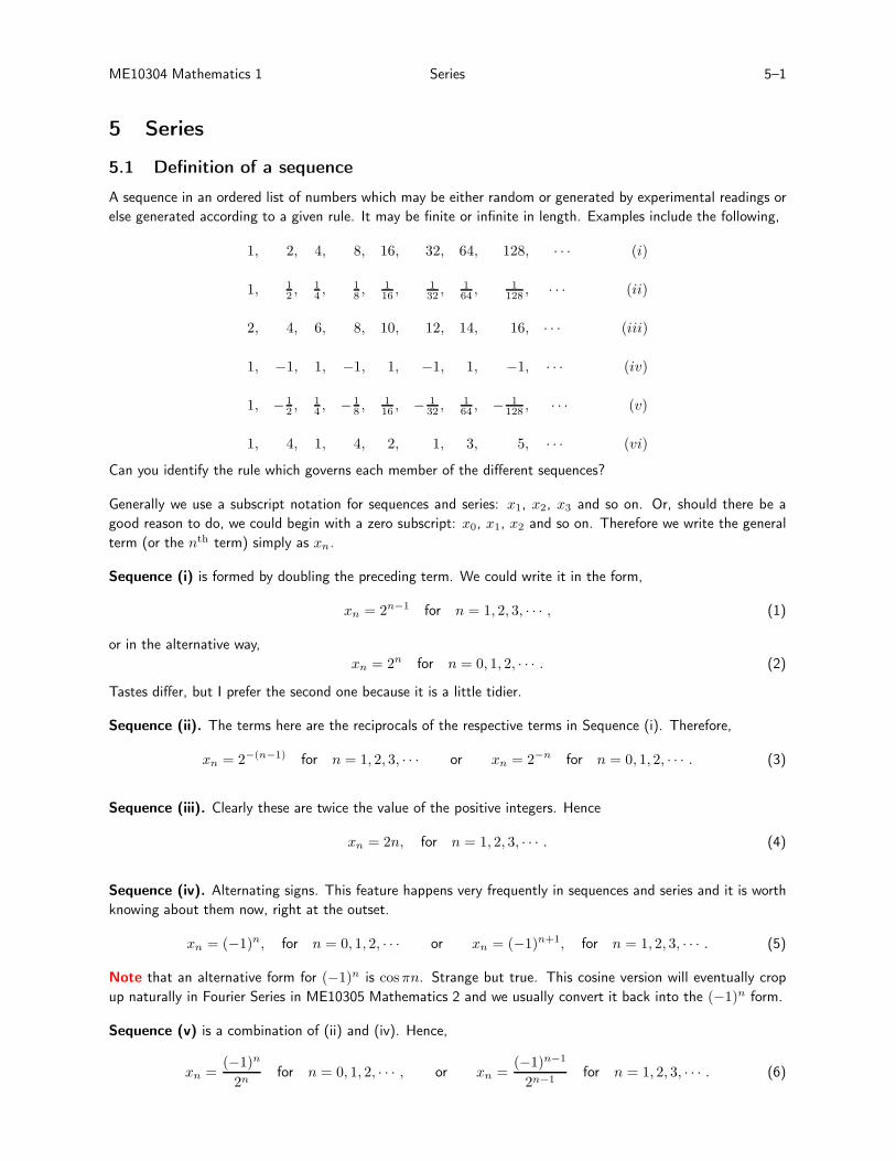
We may find an alternative form for (x + y)2 easily by multiplying out the brackets in (x + y)(x + y); it is

x2 + 2xy + y2. This fact may be visualised by means of the area of the following square.

xy

xy

y2

x2x

y

x y

Figure 5.1. Illustrating the binomial expansion of (x+y)2 using areas within a square of side, (x+y).

Further multiplication by an (x+ y) factor yields

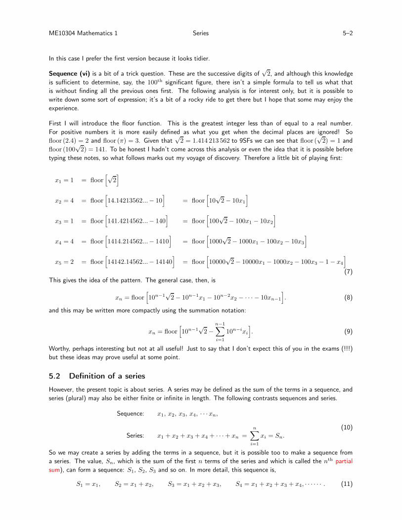
(x+ y)3 = (x+ y)(x2 + 2xy + y2) = x3 + 3x2y + 3xy2 + y3.

This again may be visualised by means of the volume of a suitable cube.


x2y

x2y

x2y

xy2

x3

y3

xy2

x

y

x y

x

y

Figure 5.2. Illustrating the binomial expansion of (x+ y)3 using cuboids.

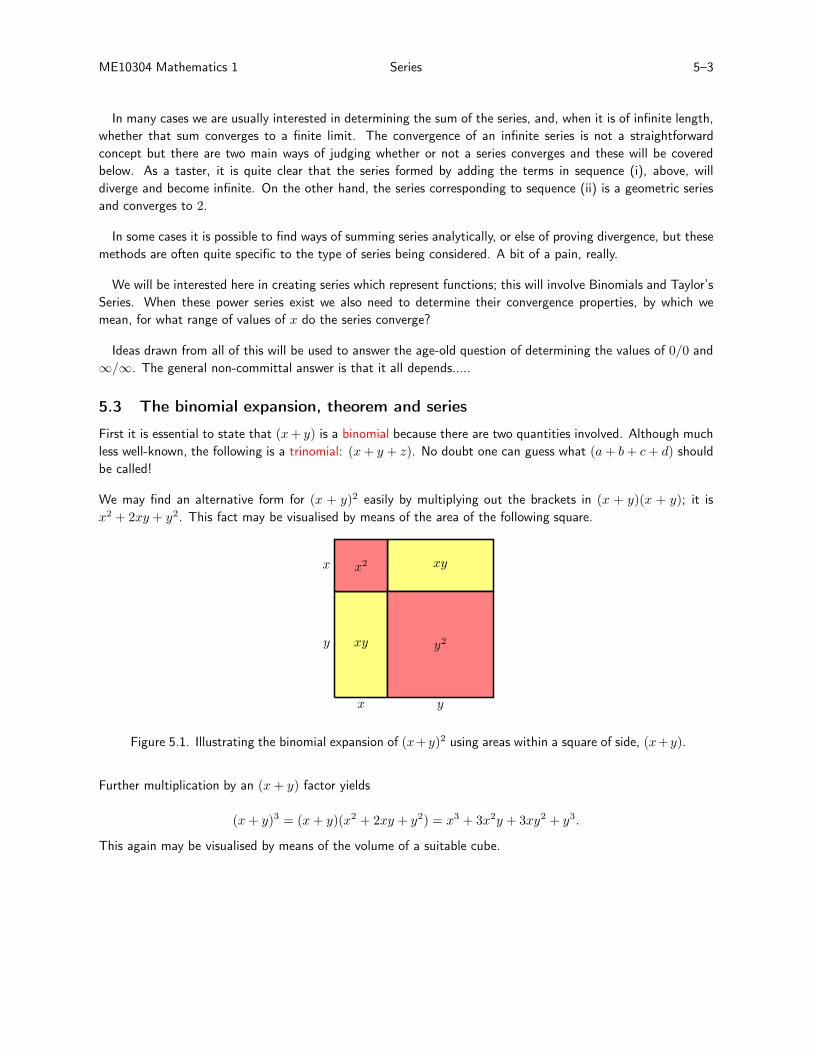
Finding higher powers is tedious, and we run out of dimensions with which to visualise them. Fortunately Pascal’s

triangle allows us to calculate fairly quickly the next few sets of coefficients. It is

n

0 : 1

1 : 1 1

2 : 1 2 1

3 : 1 3 3 1

4 : 1 4 6 4 1

5 : 1 5 10 10 5 1

6 : 1 6 15 20 15 6 1

Figure 5.3. Pascal’s triangle, which is one method for evaluating the Binomial coefficients. The red

coefficient on row 5 is the sum of the two in red on row 4; this is a property of the pattern.

So if we take the line 5 then the corresponding row of coefficients is equivalent to

(x+ y)5 = x5 + 5x4y + 10x3y2 + 10x2y3 + 5xy4 + y5. (12)

The coloured data in Pascal’s triangle illustrates the well-known property that any entry is the sum of the two

just above. That this is so is a simple consequence of multiplying by (x+ y):

(

x4 + 4x3y + 6x2y2 + 4xy3 + y4)(

x + y)

= x5 + 5x4y + 10x3y2 + 10x2y3 + 5xy4 + y5. (13)

Here we add the product of the two red terms and the product of the blue terms on the left to give the purple

term on the right, and this demonstrates the addition-of-previous-coefficients property of the Triangle.

Example 5.1. The binomial expansion may be used as a means of computing quick approximations by hand.

For example, if we set x = 1 and y = 0.01 in (12) we get

(1.01)5 = 15 + [5× 14 × 0.01] + [10× 13 × 0.012] + · · ·= 1 + 0.05 + 0.001 + · · ·≃ 1.051.

(14)


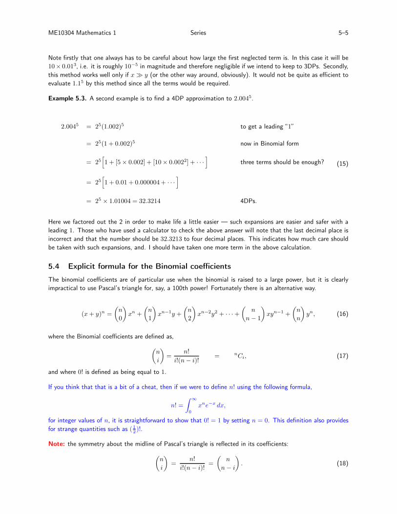
Note firstly that one always has to be careful about how large the first neglected term is. In this case it will be

10× 0.013, i.e. it is roughly 10−5 in magnitude and therefore negligible if we intend to keep to 3DPs. Secondly,

this method works well only if x ≫ y (or the other way around, obviously). It would not be quite as efficient to

evaluate 1.15 by this method since all the terms would be required.

Example 5.3. A second example is to find a 4DP approximation to 2.0045.

2.0045 = 25(1.002)5 to get a leading “1”

= 25(1 + 0.002)5 now in Binomial form

= 25[

1 + [5× 0.002] + [10× 0.0022] + · · ·]

three terms should be enough?

= 25[

1 + 0.01 + 0.000004+ · · ·]

= 25 × 1.01004 = 32.3214 4DPs.

(15)

Here we factored out the 2 in order to make life a little easier — such expansions are easier and safer with a

leading 1. Those who have used a calculator to check the above answer will note that the last decimal place is

incorrect and that the number should be 32.3213 to four decimal places. This indicates how much care should

be taken with such expansions, and. I should have taken one more term in the above calculation.

5.4 Explicit formula for the Binomial coefficients

The binomial coefficients are of particular use when the binomial is raised to a large power, but it is clearly

impractical to use Pascal’s triangle for, say, a 100th power! Fortunately there is an alternative way.

(x+ y)n =

(

n

0

)

xn +

(

n

1

)

xn−1y +

(

n

2

)

xn−2y2 + · · ·+(

n

n− 1

)

xyn−1 +

(

n

n

)

yn, (16)

where the Binomial coefficients are defined as,

(

n

i

)

=n!

i!(n− i)!= nCi, (17)

and where 0! is defined as being equal to 1.

If you think that that is a bit of a cheat, then if we were to define n! using the following formula,

n! =

∫

∞

0

xne−x dx,

for integer values of n, it is straightforward to show that 0! = 1 by setting n = 0. This definition also provides

for strange quantities such as (12 )!.

Note: the symmetry about the midline of Pascal’s triangle is reflected in its coefficients:

(

n

i

)

=n!

i!(n− i)!=

(

n

n− i

)

. (18)


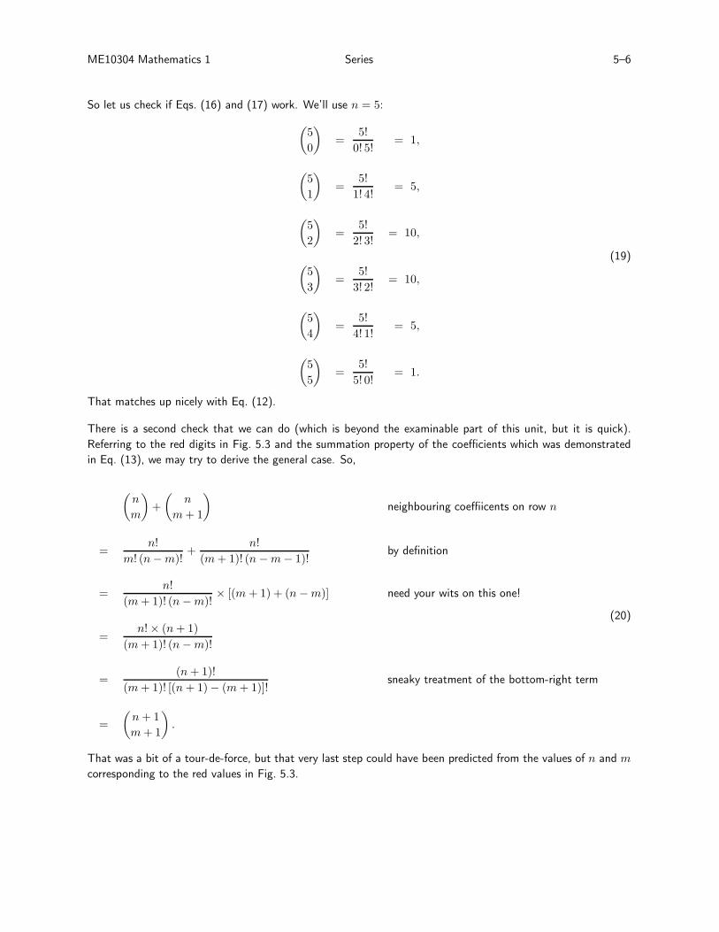
So let us check if Eqs. (16) and (17) work. We’ll use n = 5:

(

5

0

)

=5!

0! 5!= 1,

(

5

1

)

=5!

1! 4!= 5,

(

5

2

)

=5!

2! 3!= 10,

(

5

3

)

=5!

3! 2!= 10,

(

5

4

)

=5!

4! 1!= 5,

(

5

5

)

=5!

5! 0!= 1.

(19)

That matches up nicely with Eq. (12).

There is a second check that we can do (which is beyond the examinable part of this unit, but it is quick).

Referring to the red digits in Fig. 5.3 and the summation property of the coefficients which was demonstrated

in Eq. (13), we may try to derive the general case. So,

(

n

m

)

+

(

n

m+ 1

)

neighbouring coeffiicents on row n

=n!

m! (n−m)!+

n!

(m+ 1)! (n−m− 1)!by definition

=n!

(m+ 1)! (n−m)!× [(m+ 1) + (n−m)] need your wits on this one!

=n!× (n+ 1)

(m+ 1)! (n−m)!

=(n+ 1)!

(m+ 1)! [(n+ 1)− (m+ 1)]!sneaky treatment of the bottom-right term

=

(

n+ 1

m+ 1

)

.

(20)

That was a bit of a tour-de-force, but that very last step could have been predicted from the values of n and m

corresponding to the red values in Fig. 5.3.


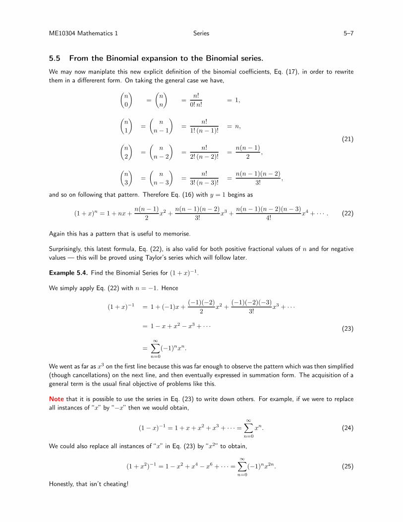
5.5 From the Binomial expansion to the Binomial series.

We may now maniplate this new explicit definition of the binomial coefficients, Eq. (17), in order to rewrite

them in a differerent form. On taking the general case we have,

(

n

0

)

=

(

n

n

)

=n!

0!n!= 1,

(

n

1

)

=

(

n

n− 1

)

=n!

1! (n− 1)!= n,

(

n

2

)

=

(

n

n− 2

)

=n!

2! (n− 2)!=

n(n− 1)

2,

(

n

3

)

=

(

n

n− 3

)

=n!

3! (n− 3)!=

n(n− 1)(n− 2)

3!,

(21)

and so on following that pattern. Therefore Eq. (16) with y = 1 begins as

(1 + x)n = 1 + nx+n(n− 1)

2x2 +

n(n− 1)(n− 2)

3!x3 +

n(n− 1)(n− 2)(n− 3)

4!x4 + · · · . (22)

Again this has a pattern that is useful to memorise.

Surprisingly, this latest formula, Eq. (22), is also valid for both positive fractional values of n and for negative

values — this will be proved using Taylor’s series which will follow later.

Example 5.4. Find the Binomial Series for (1 + x)−1.

We simply apply Eq. (22) with n = −1. Hence

(1 + x)−1 = 1 + (−1)x+(−1)(−2)

2x2 +

(−1)(−2)(−3)

3!x3 + · · ·

= 1− x+ x2 − x3 + · · ·

=∞∑

n=0

(−1)nxn.

(23)

We went as far as x3 on the first line because this was far enough to observe the pattern which was then simplified

(though cancellations) on the next line, and then eventually expressed in summation form. The acquisition of a

general term is the usual final objective of problems like this.

Note that it is possible to use the series in Eq. (23) to write down others. For example, if we were to replace

all instances of “x” by “−x” then we would obtain,

(1− x)−1 = 1 + x+ x2 + x3 + · · · =∞∑

n=0

xn. (24)

We could also replace all instances of “x” in Eq. (23) by “x2” to obtain,

(1 + x2)−1 = 1− x2 + x4 − x6 + · · · =∞∑

n=0

(−1)nx2n. (25)

Honestly, that isn’t cheating!


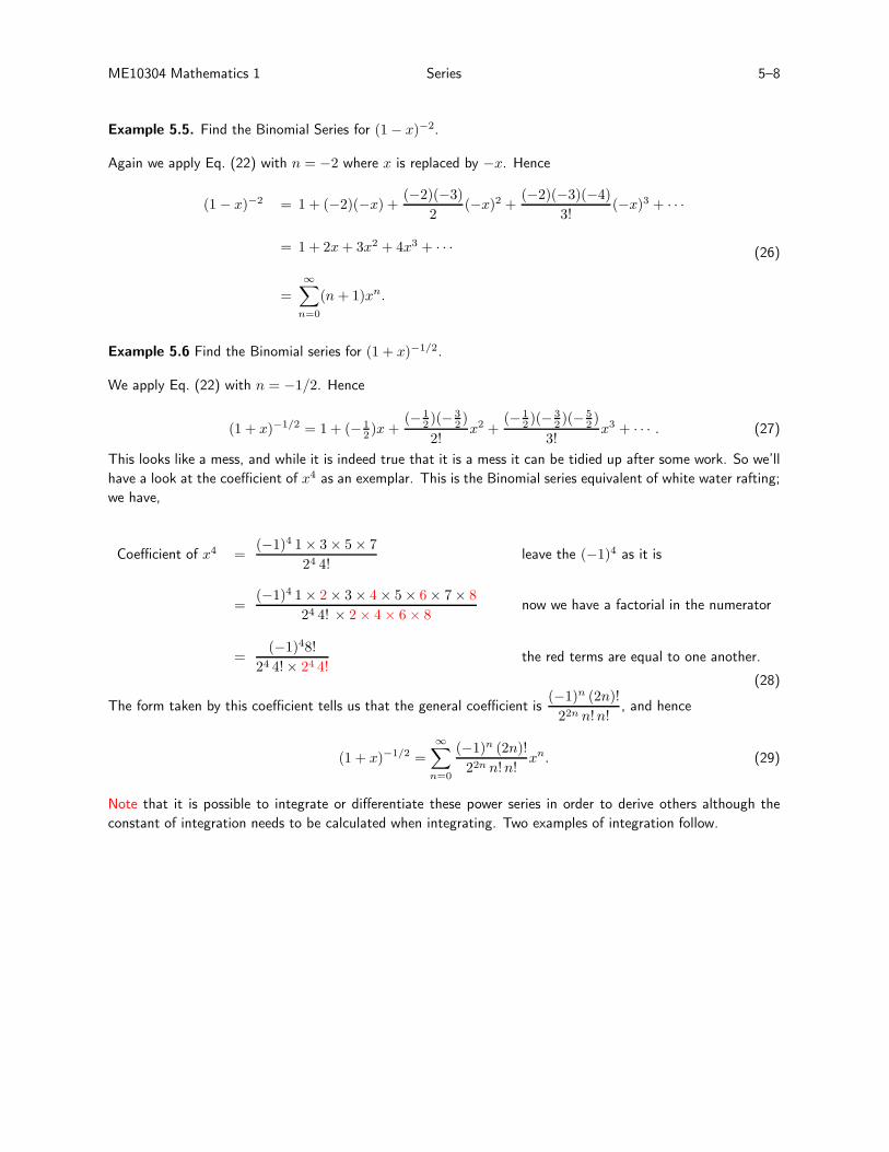
Example 5.5. Find the Binomial Series for (1 − x)−2.

Again we apply Eq. (22) with n = −2 where x is replaced by −x. Hence

(1 − x)−2 = 1 + (−2)(−x) +(−2)(−3)

2(−x)2 +

(−2)(−3)(−4)

3!(−x)3 + · · ·

= 1 + 2x+ 3x2 + 4x3 + · · ·

=∞∑

n=0

(n+ 1)xn.

(26)

Example 5.6 Find the Binomial series for (1 + x)−1/2.

We apply Eq. (22) with n = −1/2. Hence

(1 + x)−1/2 = 1+ (− 12 )x +

(− 12 )(− 3

2 )

2!x2 +

(− 12 )(− 3

2 )(− 52 )

3!x3 + · · · . (27)

This looks like a mess, and while it is indeed true that it is a mess it can be tidied up after some work. So we’ll

have a look at the coefficient of x4 as an exemplar. This is the Binomial series equivalent of white water rafting;

we have,

Coefficient of x4 =(−1)4 1× 3× 5× 7

24 4!leave the (−1)4 as it is

=(−1)4 1× 2× 3× 4× 5× 6× 7× 8

24 4! × 2× 4× 6× 8now we have a factorial in the numerator

=(−1)48!

24 4!× 24 4!the red terms are equal to one another.

(28)

The form taken by this coefficient tells us that the general coefficient is(−1)n (2n)!

22n n!n!, and hence

(1 + x)−1/2 =

∞∑

n=0

(−1)n (2n)!

22n n!n!xn. (29)

Note that it is possible to integrate or differentiate these power series in order to derive others although the

constant of integration needs to be calculated when integrating. Two examples of integration follow.


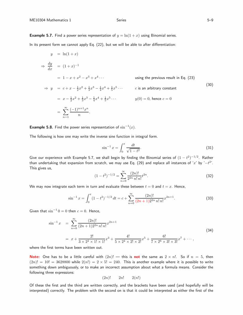
Example 5.7. Find a power series representation of y = ln(1 + x) using Binomial series.

In its present form we cannot apply Eq. (22), but we will be able to after differentiation:

y = ln(1 + x)

⇒ dy

dx= (1 + x)−1

= 1− x+ x2 − x3 + x4 · · · using the previous result in Eq. (23)

⇒ y = c+ x− 12x

2 + 13x

3 − 14x

4 + 15x

5 · · · c is an arbitrary constant

= x− 12x

2 + 13x

3 − 14x

4 + 15x

5 · · · y(0) = 0, hence c = 0

=

∞∑

n=1

(−1)n+1xn

n.

(30)

Example 5.8. Find the power series representation of sin−1(x).

The following is how one may write the inverse sine function in integral form.

sin−1 x =

∫ x

0

dt√1− t2

. (31)

Give our experience with Example 5.7, we shall begin by finding the Binomial series of (1 − t2)−1/2. Rather

than undertaking that expansion from scratch, we may use Eq. (29) and replace all instances of ‘x’ by ‘−t2’.

This gives us,

(1 − t2)−1/2 =

∞∑

n=0

(2n)!

22n n!n!t2n. (32)

We may now integrate each term in turn and evaluate these between t = 0 and t = x. Hence,

sin−1 x =

∫ x

0

(1− t2)−1/2 dt = c+

∞∑

n=0

(2n)!

(2n+ 1)22n n!n!x2n+1. (33)

Given that sin−1 0 = 0 then c = 0. Hence,

sin−1 x =

∞∑

n=0

(2n)!

(2n+ 1)22n n!n!x2n+1

= x+2!

3× 22 × 1!× 1!x3 +

4!

5× 24 × 2!× 2!x5 +

6!

7× 26 × 3!× 3!x7 + · · · ,

(34)

where the first terms have been written out.

Note: One has to be a little careful with (2n)! — this is not the same as 2 × n!. So if n = 5, then

(2n)! = 10! = 3628800 while 2(n!) = 2 × 5! = 240. This is another example where it is possible to write

something down ambiguously, or to make an incorrect assumption about what a formula means. Consider the

following three expressions:

(2n)! 2n! 2(n!)

Of these the first and the third are written correctly, and the brackets have been used (and hopefully will be

interpreted) correctly. The problem with the second on is that it could be interpreted as either the first of the


third, and therefore my recommendation is that it should never be used. One could fit the act of taking factorials

into the BODMAS/PEMDAS/BEMAS/BIDMAS rules by saying that it has a higher priority than multiplication

and division. In that case 2n! ought to be the double of n!, but I still think that it is open to misinterpretation

and therefore it should be avoided.

5.6 Power series, Maclaurin’s series and Taylor’s series

Any series of the type

a0 + a1x+ a2x2 + a3x

3 + a4x4 + · · · (35)

is called a power series simply because it consists of powers of x. An example of such a series is

cosx = 1− x2

2!+

x4

4!− x6

6!+ · · · =

∞∑

n=0

(−1)nx2n

(2n)!, (36)

but how is such an expression obtained, particularly since we cannot use the Binomial expansion?

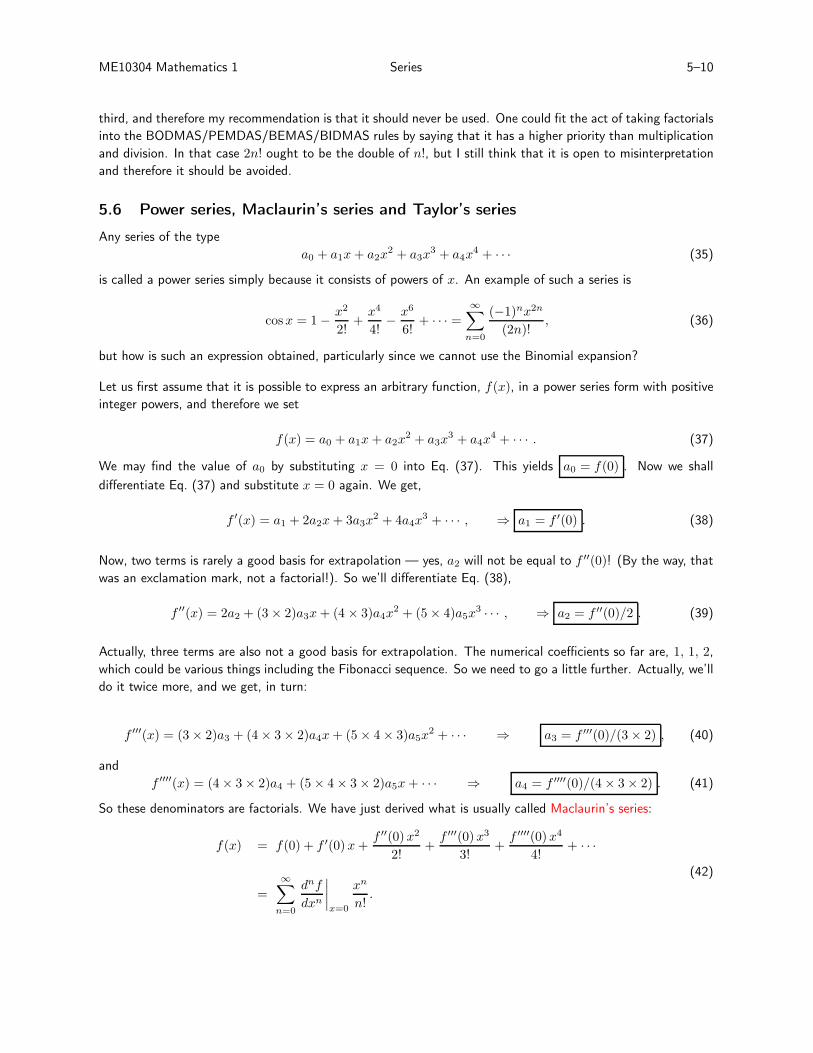
Let us first assume that it is possible to express an arbitrary function, f(x), in a power series form with positive

integer powers, and therefore we set

f(x) = a0 + a1x+ a2x2 + a3x

3 + a4x4 + · · · . (37)

We may find the value of a0 by substituting x = 0 into Eq. (37). This yields a0 = f(0) . Now we shall

differentiate Eq. (37) and substitute x = 0 again. We get,

f ′(x) = a1 + 2a2x+ 3a3x2 + 4a4x

3 + · · · , ⇒ a1 = f ′(0) . (38)

Now, two terms is rarely a good basis for extrapolation — yes, a2 will not be equal to f ′′(0)! (By the way, that

was an exclamation mark, not a factorial!). So we’ll differentiate Eq. (38),

f ′′(x) = 2a2 + (3× 2)a3x+ (4 × 3)a4x2 + (5× 4)a5x

3 · · · , ⇒ a2 = f ′′(0)/2 . (39)

Actually, three terms are also not a good basis for extrapolation. The numerical coefficients so far are, 1, 1, 2,

which could be various things including the Fibonacci sequence. So we need to go a little further. Actually, we’ll

do it twice more, and we get, in turn:

f ′′′(x) = (3× 2)a3 + (4× 3× 2)a4x+ (5× 4× 3)a5x2 + · · · ⇒ a3 = f ′′′(0)/(3× 2) , (40)

and

f ′′′′(x) = (4× 3× 2)a4 + (5× 4× 3× 2)a5x+ · · · ⇒ a4 = f ′′′′(0)/(4× 3× 2) . (41)

So these denominators are factorials. We have just derived what is usually called Maclaurin’s series:

f(x) = f(0) + f ′(0)x+f ′′(0)x2

2!+

f ′′′(0)x3

3!+

f ′′′′(0)x4

4!+ · · ·

=

∞∑

n=0

dnf

dxn

∣

∣

∣

∣

x=0

xn

n!.

(42)


The Maclaurin expansion focuses on x = 0 as the point ‘about which’ the function is expanded. More generally

we may expand about any other point, and therefore we could also have

f(x) = f(a) + f ′(a) (x− a) +f ′′(a) (x − a)2

2!+

f ′′′(a) (x− a)3

3!+

f ′′′′(a) (x − a)4

4!+ · · ·

=∞∑

n=0

dnf

dxn

∣

∣

∣

∣

x=a

(x− a)n

n!.

(43)

Equation (43) may also be derived in exactly the same way as for Eq. (42), namely by successive differentiation

and substitution of x = a. This more general expression is called Taylor’s series about x = a. Thus Maclaurin’s

series is simply Taylor’s series about x = 0.

Note: that while Eq. (43) is the one which we shall use for this unit, the University’s Formula Book has it

written down slightly differently; it is

f(x) = f(x0) + δf ′(x0) +δ2

2!f ′′(x0) +

δ3

3!f ′′′(x0) · · ·+

δn

n!f (n)(x0) +Rn+1. (44)

In this expression f (n) is the nth derivative, δ = x − x0 and the value, Rn+1 is the error due to using only a

finite series. Clearly x0 plays the same role that a does in the above analysis, but we will not be considering the

error term.

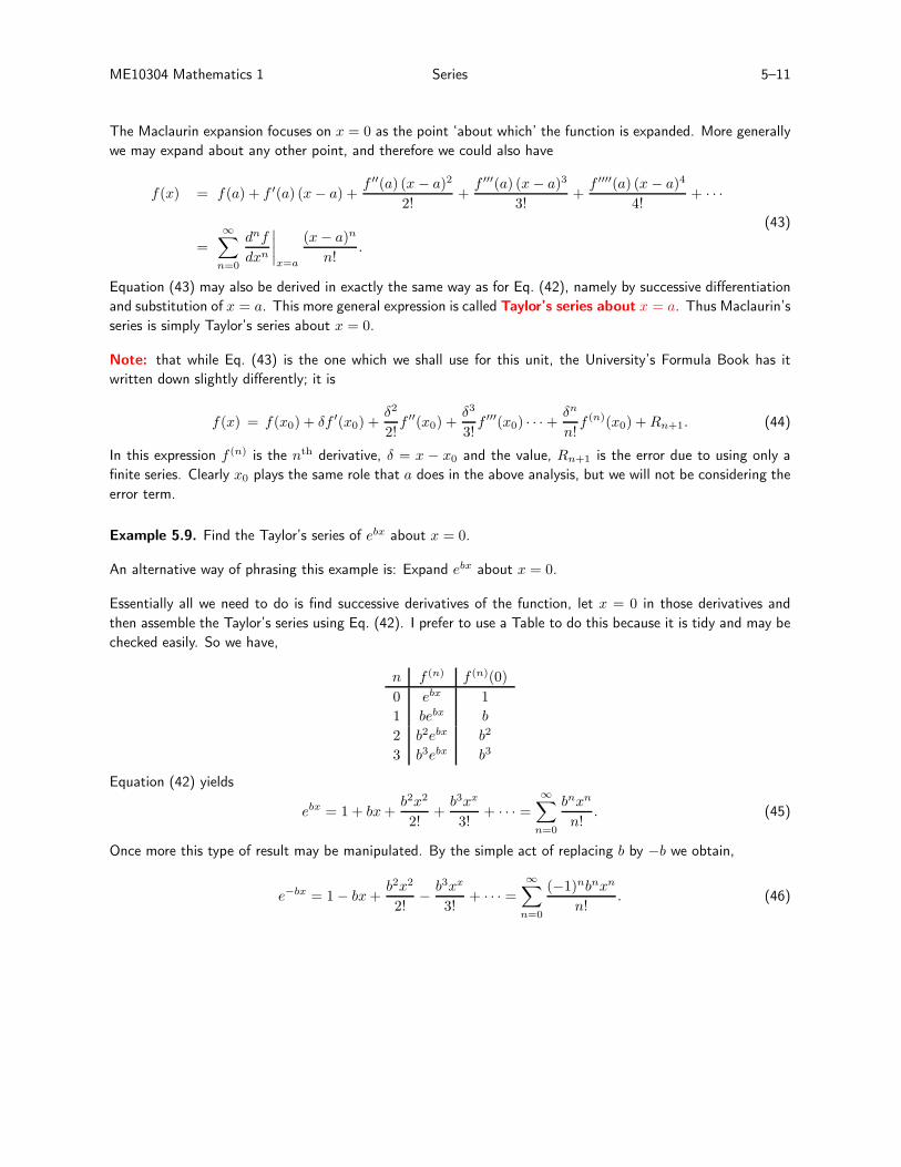
Example 5.9. Find the Taylor’s series of ebx about x = 0.

An alternative way of phrasing this example is: Expand ebx about x = 0.

Essentially all we need to do is find successive derivatives of the function, let x = 0 in those derivatives and

then assemble the Taylor’s series using Eq. (42). I prefer to use a Table to do this because it is tidy and may be

checked easily. So we have,

n f (n) f (n)(0)

0 ebx 1

1 bebx b

2 b2ebx b2

3 b3ebx b3

Equation (42) yields

ebx = 1 + bx+b2x2

2!+

b3xx

3!+ · · · =

∞∑

n=0

bnxn

n!. (45)

Once more this type of result may be manipulated. By the simple act of replacing b by −b we obtain,

e−bx = 1− bx+b2x2

2!− b3xx

3!+ · · · =

∞∑

n=0

(−1)nbnxn

n!. (46)


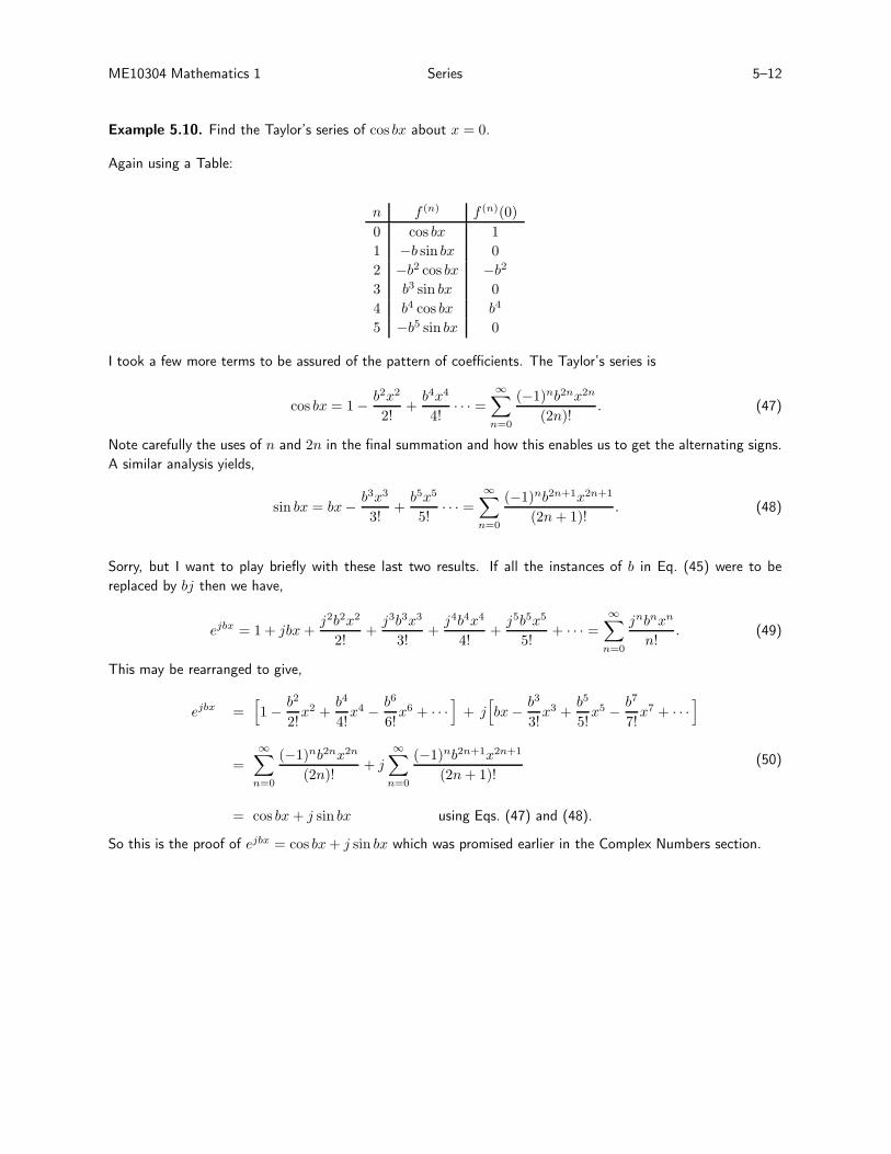
Example 5.10. Find the Taylor’s series of cos bx about x = 0.

Again using a Table:

n f (n) f (n)(0)

0 cos bx 1

1 −b sin bx 0

2 −b2 cos bx −b2

3 b3 sin bx 0

4 b4 cos bx b4

5 −b5 sin bx 0

I took a few more terms to be assured of the pattern of coefficients. The Taylor’s series is

cos bx = 1− b2x2

2!+

b4x4

4!· · · =

∞∑

n=0

(−1)nb2nx2n

(2n)!. (47)

Note carefully the uses of n and 2n in the final summation and how this enables us to get the alternating signs.

A similar analysis yields,

sin bx = bx− b3x3

3!+

b5x5

5!· · · =

∞∑

n=0

(−1)nb2n+1x2n+1

(2n+ 1)!. (48)

Sorry, but I want to play briefly with these last two results. If all the instances of b in Eq. (45) were to be

replaced by bj then we have,

ejbx = 1 + jbx+j2b2x2

2!+

j3b3x3

3!+

j4b4x4

4!+

j5b5x5

5!+ · · · =

∞∑

n=0

jnbnxn

n!. (49)

This may be rearranged to give,

ejbx =[

1− b2

2!x2 +

b4

4!x4 − b6

6!x6 + · · ·

]

+ j[

bx− b3

3!x3 +

b5

5!x5 − b7

7!x7 + · · ·

]

=∞∑

n=0

(−1)nb2nx2n

(2n)!+ j

∞∑

n=0

(−1)nb2n+1x2n+1

(2n+ 1)!

= cos bx+ j sin bx using Eqs. (47) and (48).

(50)

So this is the proof of ejbx = cos bx+ j sin bx which was promised earlier in the Complex Numbers section.


Example 5.11. Find the Taylor’s series of (1 + x)−1 about x = 0 and about x = 1.

Here’s the Table of data for the two cases:

n f (n) f (n)(0) f (n)(1)

0 (1 + x)−1 1 1/2

1 −(1 + x)−2 −1 −1/22

2 2(1 + x)−3 2 2/23

3 −3! (1 + x)−4 −3! −3!/24

4 4! (1 + x)−5 4! 4!/25

5 −5! (1 + x)−6 −5! −5!/26

From these data and Eq. (43) we obtain the desired Taylor’s series:

1

1 + x= 1− x+ x2 − x3 + x4 − x5 + · · · =

∞∑

n=0

(−1)nxn, (51)

and

1

1 + x=

1

2

[

1− x− 1

2+

(x− 1)2

22− (x− 1)3

23+

(x − 1)4

24− (x− 1)5

25+ · · ·

]

=1

2

∞∑

n=0

(−1)n(x − 1)n

2n. (52)

Example 5.12 Expand the integral y(x) =

∫ x

0

e−t2 dt about x = 0 and hence evaluate y(0.2).

This integral is very closely related to the Normal Distribution but the indefinite integral of e−x2

cannot be written

in terms of familiar functions, which is a bit awkward. Bizarrely, it is possible to show that y(x) → √π/2 as

x → ∞.

We begin by differentiating the integral; we get

y′(x) = e−x2

,

an exponential function. Now, I would not advise trying to apply the Taylor’s series formula directly. Rather it

is better to note that we already have a Taylor’s series representation of e−x in Eq. (45) and therefore we may

simply replace all occurrences of x by x2 to find that,

y′(x) = 1− x2 +x4

2!− x6

3!+

x8

4!· · · . (53)

Integration of this (noting that y(0) = 0 so that we can evaluate the constant of integration) yields,

y(x) = x− x3

3+

x5

5.2!− x7

7.3!+

x9

9.4!· · · =

∞∑

n=0

(−1)nx2n+1

(2n+ 1)× n!. (54)

Three terms of this series gives y(0.2) = 0.1974. The fourth term has magnitude 3× 10−7 and therefore these

three terms are enough.


5.7 The convergence of power series

Following on from Example 5.12 a natural question is whether we can use any value of x in Eq. (54). It is this

which forms the topic of the present section, but we will study a couple of series from earlier in this chapter

in order to illustrate that different power series may have different convergence properties. For convenience

Eqs. (51), (48) (with b = 1) and (45) (also with b = 1) are quoted here:

1

1 + x= 1− x+ x2 − x3 + x4 − x5 + · · · , (55)

sinx = x− x3

3!+

x5

5!− x7

7!+ · · · (56)

ex = 1 + x+x2

2!+

x3

3!+

x4

4!+ · · · (57)

5.7.1 Numerical demonstration of convergence/divergence

The series in Eq. (55) is a geometric series and therefore we could have found its sum, the left hand side, using

those ideas. When we choose x = 0.1 then it feels certain that the right hand side will converge because the

successive terms are decreasing rapidly. Even more obvious is the choice, x = −0.1, for then the partial sums

become, 1, 1.1, 1.11, 1.111 and on to the value 10/9. On the other hand, if we were to choose x = 2 then the

series looks like,

1− 2 + 22 − 23 + 24 − 25 + · · ·

and there is no hope of this converging to a finite value. Although the signs alternate, the magnitude of the

partial sums increase: 1, −1, 3, −5, 11,−21, 43.... After a bit of work I determined that this sequence satisfies

[(−1)22n+1 + 1]/3 — big deal! Our conclusion is that convergence for the series in Eq. (55) is conditional: if

x is small enough then it converges, but it will diverge otherwise. The boundary between those behaviours is

likely to be x = 1 for then the series is

1− 1 + 1− 1 + 1 · · · ,

and the partials sums alternate: 1, 0, 1, 0, and so on.

A similar playing around with numbers for Eqs. (56) and (57) using a calculator takes time. The fact that the

denominators are factorials gives a hint that these series might be convergent. If one were to choose x = 0.1 in

Eq. (57), then only a few terms are required to obtain, say, 6DP accuracy. This may be seen in the following

Table (where un represents the successive terms, and Sn the partial sums):

Showing successive terms and partial sums for Eq. (57) when x = 0.1

n un Sn

0 1.000000 1.000000

1 0.100000 1.100000

2 0.005000 1.105000

3 0.000167 1.105167

4 0.000004 1.105171

5 4× 10−7 1.105171

That final answer is correct to 6DPs.

On the other hand, if we choose x = 10 then we will have the following.


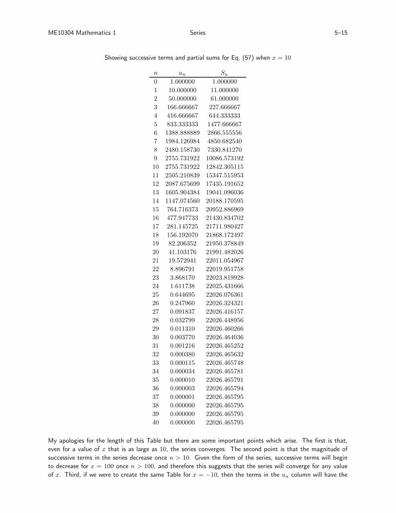
Showing successive terms and partial sums for Eq. (57) when x = 10

n un Sn

0 1.000000 1.000000

1 10.000000 11.000000

2 50.000000 61.000000

3 166.666667 227.666667

4 416.666667 644.333333

5 833.333333 1477.666667

6 1388.888889 2866.555556

7 1984.126984 4850.682540

8 2480.158730 7330.841270

9 2755.731922 10086.573192

10 2755.731922 12842.305115

11 2505.210839 15347.515953

12 2087.675699 17435.191652

13 1605.904384 19041.096036

14 1147.074560 20188.170595

15 764.716373 20952.886969

16 477.947733 21430.834702

17 281.145725 21711.980427

18 156.192070 21868.172497

19 82.206352 21950.378849

20 41.103176 21991.482026

21 19.572941 22011.054967

22 8.896791 22019.951758

23 3.868170 22023.819928

24 1.611738 22025.431666

25 0.644695 22026.076361

26 0.247960 22026.324321

27 0.091837 22026.416157

28 0.032799 22026.448956

29 0.011310 22026.460266

30 0.003770 22026.464036

31 0.001216 22026.465252

32 0.000380 22026.465632

33 0.000115 22026.465748

34 0.000034 22026.465781

35 0.000010 22026.465791

36 0.000003 22026.465794

37 0.000001 22026.465795

38 0.000000 22026.465795

39 0.000000 22026.465795

40 0.000000 22026.465795

My apologies for the length of this Table but there are some important points which arise. The first is that,

even for a value of x that is as large as 10, the series converges. The second point is that the magnitude of

successive terms in the series decrease once n > 10. Given the form of the series, successive terms will begin

to decrease for x = 100 once n > 100, and therefore this suggests that the series will converge for any value

of x. Third, if we were to create the same Table for x = −10, then the terms in the un column will have the


same magnitude as these but will alternate in sign. Despite the cancellations due to having both positive and

negative values with a large magnitude, the final converged value of this series is e−10 ≃ 0.00004540 which is

the same value that I get on my calculator.

For a more extreme case, x = −40, the ‘converged’ value of the series turns out to be about −3.166 which

is clearly wrong — exponentials can’t be negative. So what has happened? This has arisen because the 13

significant figures of accuracy in my computer calculations are no longer sufficient to cope with the great amount

of cancellations that arise when adding the terms in the series. For x = −40 my calculator gives 4.248× 10−18

which I have checked to be correct via other means, and therefore I conclude that my calculator doesn’t use

Taylor’s series! Even here, one must always be aware of significant figures and whether accuracy has been

compromised because of the necessary use of finite precision arithmetic.

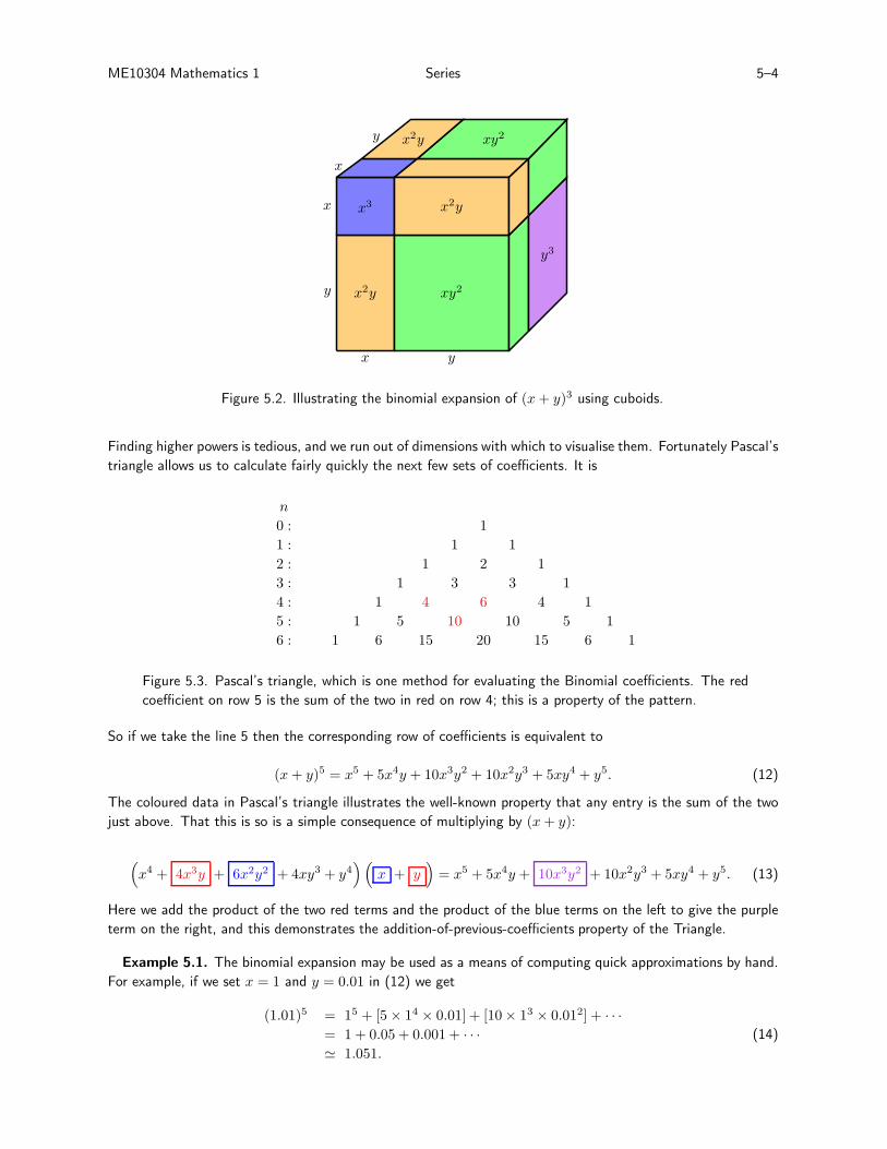
5.7.2 Graphical representation of convergence/divergence

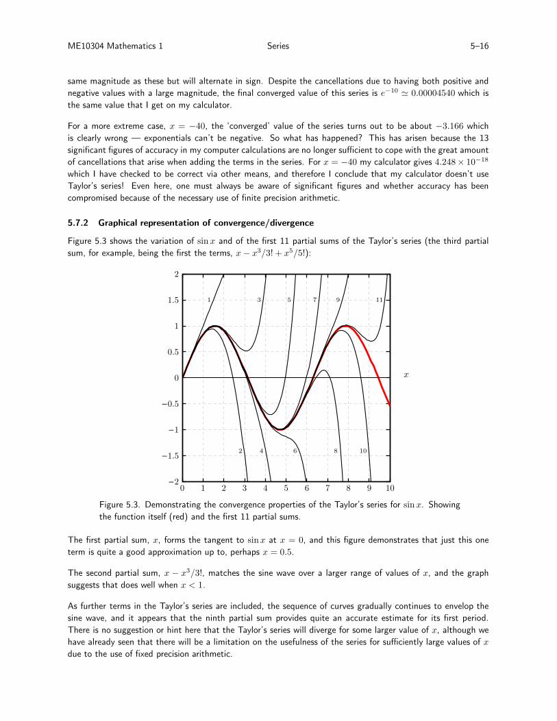
Figure 5.3 shows the variation of sinx and of the first 11 partial sums of the Taylor’s series (the third partial

sum, for example, being the first the terms, x− x3/3! + x5/5!):

0 1 2 3 4 5 6 7 8 9 10−2

−1.5

−1

−0.5

0

0.5

1

1.5

2

x

1 3 5 7 9 11

2 4 6 8 10

Figure 5.3. Demonstrating the convergence properties of the Taylor’s series for sinx. Showing

the function itself (red) and the first 11 partial sums.

The first partial sum, x, forms the tangent to sinx at x = 0, and this figure demonstrates that just this one

term is quite a good approximation up to, perhaps x = 0.5.

The second partial sum, x − x3/3!, matches the sine wave over a larger range of values of x, and the graph

suggests that does well when x < 1.

As further terms in the Taylor’s series are included, the sequence of curves gradually continues to envelop the

sine wave, and it appears that the ninth partial sum provides quite an accurate estimate for its first period.

There is no suggestion or hint here that the Taylor’s series will diverge for some larger value of x, although we

have already seen that there will be a limitation on the usefulness of the series for sufficiently large values of x

due to the use of fixed precision arithmetic.


So our tentative conclusion is that covergence happens irrespective of the value of x.

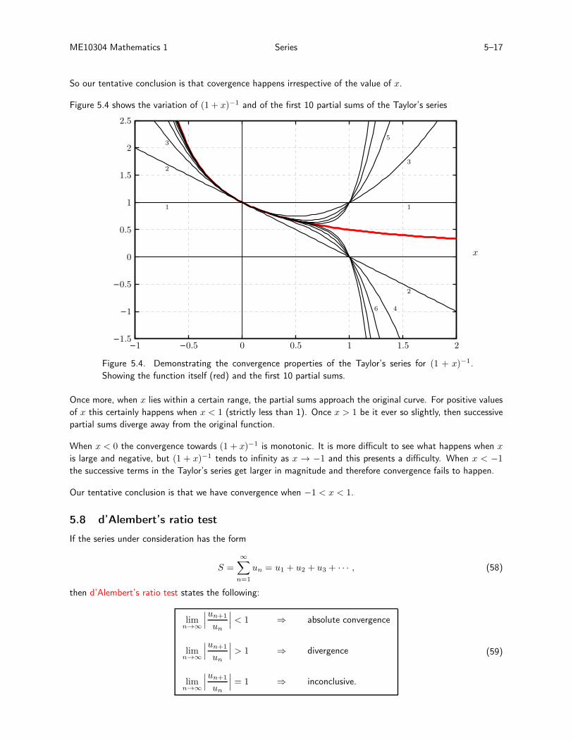
Figure 5.4 shows the variation of (1 + x)−1 and of the first 10 partial sums of the Taylor’s series

0 0.5 1 1.5 2−0.5−1−1.5

−1

−0.5

0

0.5

1

1.5

2

2.5

x

1

2

3

1

2

3

4

5

6

Figure 5.4. Demonstrating the convergence properties of the Taylor’s series for (1 + x)−1.

Showing the function itself (red) and the first 10 partial sums.

Once more, when x lies within a certain range, the partial sums approach the original curve. For positive values

of x this certainly happens when x < 1 (strictly less than 1). Once x > 1 be it ever so slightly, then successive

partial sums diverge away from the original function.

When x < 0 the convergence towards (1 + x)−1 is monotonic. It is more difficult to see what happens when x

is large and negative, but (1 + x)−1 tends to infinity as x → −1 and this presents a difficulty. When x < −1

the successive terms in the Taylor’s series get larger in magnitude and therefore convergence fails to happen.

Our tentative conclusion is that we have convergence when −1 < x < 1.

5.8 d’Alembert’s ratio test

If the series under consideration has the form

S =

∞∑

n=1

un = u1 + u2 + u3 + · · · , (58)

then d’Alembert’s ratio test states the following:

limn→∞

∣

∣

∣

un+1

un

∣

∣

∣< 1 ⇒ absolute convergence

limn→∞

∣

∣

∣

un+1

un

∣

∣

∣> 1 ⇒ divergence

limn→∞

∣

∣

∣

un+1

un

∣

∣

∣= 1 ⇒ inconclusive.

(59)


Note: that this test relies on the long-term behaviour of the coefficients, and therefore the starting point (viz.

n = 1 in Eq. (58)) is of no consequence.

d’Alembert’s test is an excellent method for finding the range of values of x for power series, but when the series

consists solely of numerical data inconclusive conclusions apply to a depressingly wide range of useful series.

You’ll see what I mean....

5.8.1 Convergence of numerical series

Example 5.13. The Maclaurin’s series for e1 is e1 = 1 +1

1!+

1

2!+

1

3!+ · · · . Determine if it converges to a

value.

The first step always is to determine an expression for the general term. In this case the general term is the

reciprocal of successive factorials. Hence Hence un = 1/n! and un+1 = 1/(n + 1)!. The second step is to

evaluate |un+1/un|:∣

∣

∣

un+1

un

∣

∣

∣=

∣

∣

∣

n!

(n+ 1)!

∣

∣

∣=

1

n+ 1. (60)

Hence,

limn→∞

∣

∣

∣

un+1

un

∣

∣

∣= lim

n→∞

1

n+ 1= 0. (61)

Given that 0 < 1, this series converges.

Example 5.14. Use d’Alembert’s test to check for the convergence of the geometric series, r + r2 + r3 + · · · .

Here un may be taken to be rn. Hence un+1 = rn+1 and so un+1/un = r. Therefore we have,

limn→∞

∣

∣

∣

un+1

un

∣

∣

∣= |r|. (62)

For convergence we require |r| < 1.

Example 5.15. Consider the sum of the reciprocals of the positive integers,

∞∑

n=1

1

n= 1 +

1

2+

1

3+

1

4+ · · · .

Here un = 1/n and therefore

∣

∣

∣

un+1

un

∣

∣

∣=

∣

∣

∣

n

n+ 1

∣

∣

∣=

1

1 + 1n

−→ 1 as n −→ ∞. (63)

Therefore the test is inconclusive.

However, it is possible to show that the series is divergent by considering the series in the following way.

1 + 12 +

(

13 + 1

4

)

+(

15 + 1

6 + 17 + 1

8

)

+(

19 + · · · 1

16

)

+ · · ·

> 1 + 12 +

(

14 + 1

4

)

+(

18 + 1

8 + 18 + 1

8

)

+(

116 + · · · 1

16

)

+ · · ·

= 1 + 12 + 1

2 + 12 + 1

2 + · · ·

(64)


Clearly this process continues indefinitely and if we continue to N such sets of brackets then we will accumulate

N instances of 12 , and therefore

S2N =

2N∑

n=1

1

n> 1 + 1

2N,

and hence the series diverges.

This is a trick that can only very rarely be deployed, but it is interesting.

Having settled the convergence properties of this example, we may return to Example 5.7 which yields the

following when x = 1 is substituted,

∞∑

n=1

(−1)n+1

n= 1− 1

2 + 13 − 1

4 + · · · .

This differs from the present example by having alternating signs, yet Example 5.7 shows that this series adds

to ln 2 and hence it is convergent.

These two series demonstrate the idea of conditional convergence. The respective magnitudes of the terms in

the two series are identical but the pattern of signs differ, so the convergence properties then depend on that

pattern of signs.

Example 5.16. Consider the sum of the reciprocals of the squares of the integers,

∞∑

n=1

1

n2= 1 +

1

22+

1

32+

1

42+ · · · .

Here un = 1/n2 and hence

∣

∣

∣

un+1

un

∣

∣

∣=

∣

∣

∣

n2

(n+ 1)2

∣

∣

∣=

1

(1 + 1n )

2−→ 1 as n −→ ∞. (65)

Again we have an inconclusive conclusion from d’Alembert! This is a little depressing for these coefficients decay

more rapidly than those in Example 5.15. This series does in fact converge, but it requires us to use Fourier

Series methods (to be done in ME10305 Mathematics 2) to show that the sum is π2/6. The equivalent sum of

the reciprocals of the fourth powers of the positive integers is π4/90, although d’Alembert’s test still remains

inconclusive even for this series.

5.9 Application of d’Alembert’s test to power series

Now we take the power series,

a0 + a1x+ a2x2 + a3x

3 + a4x4 · · · , (66)

and apply d’Alembert’s ratio test to it. Therefore we obtain convergence when

limn→∞

∣

∣

∣

an+1xn+1

anxn

∣

∣

∣< 1. (67)

Although this may be simplified and rearranged to get the convergence criterion,

|x| < limn→∞

∣

∣

∣

anan+1

∣

∣

∣. (68)

I really don’t like to teach this form because the subscripts here (n on top, n + 1 below) are the opposite way

around from those in the original ratio test given in Eq. (59) and this could be confusing. My preference is

to employ the formula in Eq. (59) as it is and then follow what the maths tells us. I will do this in all of the

examples below.


Example 5.17. Find the values of x for which the following power series converges.

1 + 2x+ 4x2 + 8x3 + 16x4 + · · · .

The general term may be written as un = 2nxn and therefore we have∣

∣

∣

un+1

un

∣

∣

∣=

∣

∣

∣

2n+1xn+1

2nxn

∣

∣

∣= 2|x|. (69)

Therefore we have convergence when 2|x| < 1, or when |x| < 12 . So for this series the radius of convergence

is 12 . Thus values of x which are larger than 1

2 in magnitude will cause the series to diverge.

Note: that this is called a radius of convergence because the result also applies for general complex values of

x, and therefore the region of convergence in the complex plane is indeed a circle.

Example 5.18. Find the values of x for which the Taylor series given in Eq. (52) converges.

The series is1

2

∞∑

n=0

(−1)n(x− 1)n

2n

and therefore the general term is

un =(−1)n(x− 1)n

2n.

Hence,

limn→∞

∣

∣

∣

un+1

un

∣

∣

∣= lim

n→∞

∣

∣

∣

(−1)n+1(x− 1)n+1

2n+2× 2n+1

(−1)n(x− 1)n

∣

∣

∣= lim

n→∞

∣

∣

∣

(x− 1)

2

∣

∣

∣= 1

2 |x− 1|. (70)

This needs to be less than 1 for convergence, which means that |x − 1| < 2. So the radius of convergence is

2, and should we wish to confine ourselves to real values of x, this means that convergence takes place when

−1 < x < 3.

Example 5.19. Find the radius of convergence of the Taylor’s series for ex given in Eq. (57).

The series is ex = 1 + x+ x2/2! + x3/3! + x4/4! + · · · . Hence the general term is un = xn/n!, and therefore

d’Alembert’s test gives,

limn→∞

∣

∣

∣

un+1

un

∣

∣

∣= lim

n→∞

∣

∣

∣

xn+1 n!

(n+ 1)!xn

∣

∣

∣= lim

n→∞

∣

∣

∣

x

(n+ 1)

∣

∣

∣= 0. (71)

While we saw this sort of result in Example 5.13, in the present context the limit is zero for all possible values

of x, and therefore this function has an infinite radius of convergence. This confirms our deduction from

numerical evidence in Section 5.7.1.

Example 5.20. Find the radius of convergence of the Taylor’s series for sinx which is given in Eq. (56).

The series is sinx = x− x3

3!+

x5

5!− x7

7!+ · · · and therefore the general term is un =

(−1)nx2n+1

(2n+ 1)!.

The correct expression for un+1 is(−1)n+1x2n+3

(2n+ 3)!. Note that the replacement of n by n + 1 in 2n+ 1 yields

2n+ 3 rather than 2n+ 2, a favourite error of so many undergraduates!

Hence

limn→∞

∣

∣

∣

∣

un+1

un

∣

∣

∣

∣

= limn→∞

∣

∣

∣

∣

(−1)n+1x2n+3

(2n+ 3)!× (2n+ 1)!

(−1)n+1x2n+1

∣

∣

∣

∣

= limn→∞

∣

∣

∣

∣

x2

(2n+ 3)(2n+ 2)

∣

∣

∣

∣

= 0. (72)

So again we have an infinite radius of convergence, just as we suspected from the graphical evidence in Fig. 5.3.


5.10 l’Hôpital’s rule

5.10.1 A graphical motivation

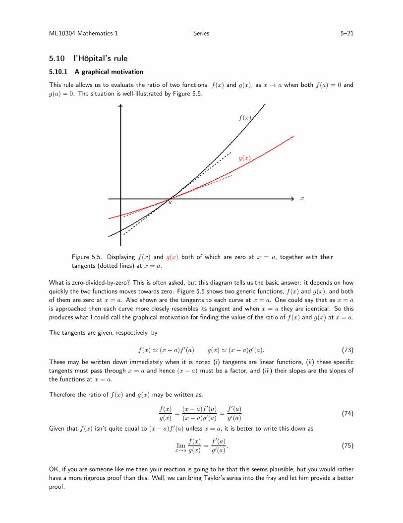
This rule allows us to evaluate the ratio of two functions, f(x) and g(x), as x → a when both f(a) = 0 and

g(a) = 0. The situation is well-illustrated by Figure 5.5.

x

f(x)

g(x)

a

Figure 5.5. Displaying f(x) and g(x) both of which are zero at x = a, together with their

tangents (dotted lines) at x = a.

What is zero-divided-by-zero? This is often asked, but this diagram tells us the basic answer: it depends on how

quickly the two functions moves towards zero. Figure 5.5 shows two generic functions, f(x) and g(x), and both

of them are zero at x = a. Also shown are the tangents to each curve at x = a. One could say that as x = a

is approached then each curve more closely resembles its tangent and when x = a they are identical. So this

produces what I could call the graphical motivation for finding the value of the ratio of f(x) and g(x) at x = a.

The tangents are given, respectively, by

f(x) ≃ (x− a)f ′(a) g(x) ≃ (x− a)g′(a). (73)

These may be written down immediately when it is noted (i) tangents are linear functions, (ii) these specific

tangents must pass through x = a and hence (x − a) must be a factor, and (iii) their slopes are the slopes of

the functions at x = a.

Therefore the ratio of f(x) and g(x) may be written as,

f(x)

g(x)=

(x− a)f ′(a)

(x− a)g′(a)=

f ′(a)

g′(a). (74)

Given that f(x) isn’t quite equal to (x− a)f ′(a) unless x = a, it is better to write this down as

limx→a

f(x)

g(x)=

f ′(a)

g′(a). (75)

OK, if you are someone like me then your reaction is going to be that this seems plausible, but you would rather

have a more rigorous proof than this. Well, we can bring Taylor’s series into the fray and let him provide a better

proof.


5.10.2 Proof of ’l’Hôpital’s rule using Taylor’s series

Equations (73) use what is, in reality, the first nonzero term of the Taylor’s series of the two functions. We need

to use a few more just to check that all is well. So let us write out this ratio again and work on it.

f(x)

g(x)= ✟

✟✟f(a) + (x− a)f ′(a) + 12 (x− a)2f ′′(a) + 1

3! (x− a)3f ′′′(a) + · · ·✟✟✟g(a) + (x− a)g′(a) + 1

2 (x− a)2g′′(a) + 13! (x− a)3g′′′(a) + · · · by definition

=f ′(a) + 1

2 (x− a)f ′′(a) + 13! (x− a)2f ′′′(a) + · · ·

g′(a) + 12 (x− a)g′′(a) + 1

3! (x− a)2g′′′(a) + · · · cancelling (x− a)

−→ f ′(a)

g′(a)as x → a.

(76)

The conclusion here is that the terms we neglected in Eq. (73) do not contribute to the final answer, but it was

necessary to check this for our peace of mind. So Eq. (75) has been retrieved using a better analysis.

Example 5.21 Find limx→0

sin 2x

x.

Both the numerator and the denominator are zero at x = 0 and therefore we apply l’Hôpital’s rule.

limx→0

sin 2x

x=

2 cos 2x

1

∣

∣

∣

x=0= 2.

Example 5.22 Find limx→π

sinx

x− π.

The numerator and the denominator are zero at x = π and therefore,

limx→π

sinx

x− π=

cosx

1

∣

∣

∣

x=π= −1.


sin2 x

x.

We have

limx→0

sin2 x

x=

2 sinx cosx

1

∣

∣

∣

x=0= 0.

This example shows that zero is a legitimate final answer.


sinx

x2.

We have

limx→0

sinx

x2=

cosx

2x

∣

∣

∣

x=0= ∞.

So this example shows that it is legitimate for an infinite solution to be obtained. One can say that x2 tends to

zero much faster than sinx does.


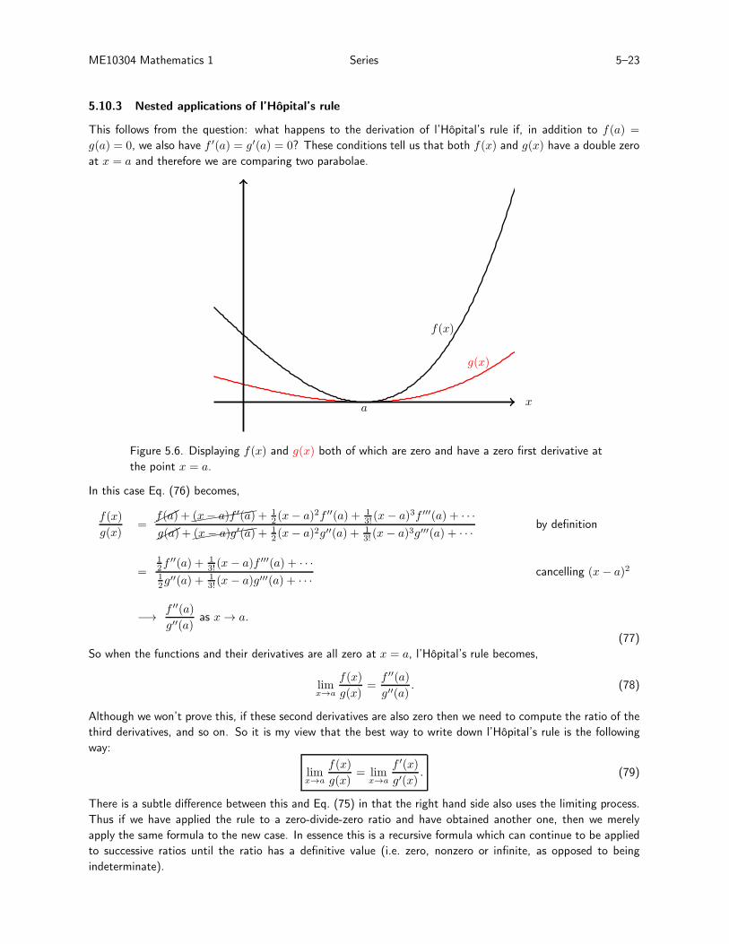
5.10.3 Nested applications of l’Hôpital’s rule

This follows from the question: what happens to the derivation of l’Hôpital’s rule if, in addition to f(a) =

g(a) = 0, we also have f ′(a) = g′(a) = 0? These conditions tell us that both f(x) and g(x) have a double zero

at x = a and therefore we are comparing two parabolae.

x

f(x)

g(x)

a

Figure 5.6. Displaying f(x) and g(x) both of which are zero and have a zero first derivative at

the point x = a.

In this case Eq. (76) becomes,

f(x)

g(x)= ✟

✟✟f(a) +✭✭✭✭✭✭(x− a)f ′(a) + 12 (x− a)2f ′′(a) + 1

3! (x− a)3f ′′′(a) + · · ·✟✟✟g(a) +✭✭✭✭✭✭(x− a)g′(a) + 1

2 (x− a)2g′′(a) + 13! (x− a)3g′′′(a) + · · · by definition

=12f

′′(a) + 13!(x − a)f ′′′(a) + · · ·

12g

′′(a) + 13!(x − a)g′′′(a) + · · · cancelling (x− a)2

−→ f ′′(a)

g′′(a)as x → a.

(77)

So when the functions and their derivatives are all zero at x = a, l’Hôpital’s rule becomes,

limx→a

f(x)

g(x)=

f ′′(a)

g′′(a). (78)

Although we won’t prove this, if these second derivatives are also zero then we need to compute the ratio of the

third derivatives, and so on. So it is my view that the best way to write down l’Hôpital’s rule is the following

way:

limx→a

f(x)

g(x)= lim

x→a

f ′(x)

g′(x). (79)

There is a subtle difference between this and Eq. (75) in that the right hand side also uses the limiting process.

Thus if we have applied the rule to a zero-divide-zero ratio and have obtained another one, then we merely

apply the same formula to the new case. In essence this is a recursive formula which can continue to be applied

to successive ratios until the ratio has a definitive value (i.e. zero, nonzero or infinite, as opposed to being

indeterminate).



1− cos ax

x2.

limx→0

1− cos ax

x2= lim

x→0

a sinax

2xThis too is a 0/0 case, hence l’H again

= limx→0

a2 cos ax

2This isn’t a 0/0 case

= 12a

2.


sinx− x

x3.

limx→0

sinx− x

x3= lim

x→0

cosx− 1

3x2This too is a 0/0 case, hence l’H again

= limx→0

− sinx

6xThis too is a 0/0 case, hence l’H again

= limx→0

− cosx

6=

1

6This isn’t a 0/0 case

5.10.4 A few more exotic examples

Example 5.27 Find limx→∞

eax

x.

This example demonstrates two different variations on the standard l’Hôpital’s rule theme. First we are con-

sidering x → ∞ and second we are considering two functions that become infinite in that limit. In this case

l’Hôpital’s rule is comparing the speed at which the two functions grow in magnitude. We have

limx→∞

eax

x=

aeax

1

∣

∣

∣

x→∞

= ∞.

Example 5.28 [A more difficult example.] Find limx→0

xx.

This doesn’t look like a l’Hôpital’s rule question because there is no ratio! However, if we let y = xx, then

ln y = x lnx =lnx

1/x.

This is an x → 0 problem where the ratio is an infinity-over-infinity case. Now we may apply l’Hôpital’s rule:

limx→0

ln y = limx→0

lnx

1/xThis is an ∞/∞ case, hence use l’H

= limx→0

1/x

−1/x2Of the same form, but we can simplify this one

= limx→0

(−x)

= 0.

Since ln y → 0 then y → 1. Therefore the x → 0 limit of xx is 1.


Example 5.29 [Also a more difficult example.] Find limn→∞

(

1 +1

n

)n

.

This problem is associated with compound interest. When n = 1 the factor (1+ 1n )

n may be said to be equivalent

to the adding of 100% interest to an investment, I, after a year. The yield is that the investment doubles to 2I.

When n = 2, 50% interest is applied twice per year, and the return is now (1 + 12 )

2I = 2.25I.

When n = 4, 25% interest is added quarterly, and the return is (1 + 14 )

4I = 2.441406I.

If monthly, then the return is (1+ 112 )

12I = 2.613035I. The ultimate question is: what is your return if interest

is added continuously at the appropriate infinitesimal rate?

Again this is not a ratio, but again we may take logs. So if y = (1 + 1n )

n then

ln y = n ln(

1 +1

n

)

=ln(

1 +1

n

)

1

n

.

This looks very messy, but with a little sleight of hand we may transform a large–n problem into a small–x

problem by setting x = 1/n. Therefore the problem becomes,

limx→0

ln(1 + x)

x= lim

x→0

1/(1 + x)

1= 1.

This, then, is the value of ln y and therefore the n → ∞ limit of y is e. The return on the investment will be

eI. You won’t get any more than that!

Documents

5 Series - University of Bath