Text Analysis Report

Text Analytics Assignment Analysis of reviews fetched from FLIPKART.COM

for MOTO-G (2nd gen)

Roma Agrawal

1/28/2015

Roma Agrawal | Introduction 1

Table of Contents

Introduction .................................................................................................................................................. 2

Web Crawling ................................................................................................................................................ 3

What is Web Crawling? ......................................................................................................................... 3

Extracted Reviews ................................................................................................................................. 3

Extracted Ratings .................................................................................................................................. 3

Analysis of Terms & Documents (TDM) ........................................................................................................ 4

Creation of Term-Document matrix ......................................................................................................... 4

What is TDM? ........................................................................................................................................ 4

What is TF-IDF? ..................................................................................................................................... 4

Word Cloud ............................................................................................................................................... 4

What is word Cloud? ............................................................................................................................. 4

Dimension Reduction ................................................................................................................................ 5

What are LSA and SVD? ........................................................................................................................ 5

The 3 matrices generated: Tk, Dk, Sk .................................................................................................... 5

Clustering .................................................................................................................................................. 9

Cluster Analysis for “Terms” ................................................................................................................. 9

Cluster Analysis for “Documents” ....................................................................................................... 11

Analysis of Ratings ...................................................................................................................................... 13

Importance of Terms on the basis of “Satisfaction” using SVM ................................................................. 14

What is Classification? ............................................................................................................................ 14

What is Support Vector Machine? .......................................................................................................... 14

Sentiment Analysis ...................................................................................................................................... 15

What is sentiment analysis and polarity? ............................................................................................... 15

Appendix ..................................................................................................................................................... 16

Bibliography ................................................................................................................................................ 20

Roma Agrawal | Introduction 2

Introduction

India’s most popular shopping site www.flipkart.com is commonly used for viewing the specifications of

electronic goods especially cell phones. Before buying any phone, people generally visit this site and

look for reviews of their products which they are planning to buy.

This report is on analysis done on reviews given by customers after using MOTO G (2nd gen) black

colored phone, a product which is ONLY available in www.flipkart.com.

We have considered reviews up to 10 pages. Each page contains 10 reviews, therefore total 100 reviews

we have taken. We have not ignored small reviews (less than 200 characters) as people may also write

their views in one liner sentence as well.

Everything is done using R-Studio

http://www.flipkart.com/


Roma Agrawal | Web Crawling 3

Web Crawling

What is Web Crawling?

A crawler is a program that retrieves and stores pages from the Web, generally used by the Web search

engines to index web pages in their systems. A crawler often has to download hundreds of millions of

pages in a short period of time and has to constantly monitor and refresh the downloaded pages. In

addition, the crawler should avoid putting too much pressure on the visited Web sites and the crawler's

local network, because they are intrinsically shared resources.

Extracted Reviews

Using this web crawling technique, we have extracted reviews for our analysis. Not all reviews are of

same length, as we have observed that in site also, some people write detailed reviews and some write

one liner to express their views, which equally have same weightage.

Extracted Ratings

With reviews, we have captured the ratings given by each customer (out of 5). The customers who have

written the reviews have also given the ratings. We have done analysis on ratings after analyzing the

documents and terms extracted from reviews.

Roma Agrawal | Analysis of Terms & Documents (TDM) 4

Analysis of Terms & Documents (TDM)

Creation of Term-Document matrix

What is TDM?

A document-term matrix or term-document matrix is a mathematical matrix that describes the

frequency of terms that occur in a collection of documents. In a document-term matrix, rows

correspond to documents in the collection and columns correspond to terms. There are various schemes

for determining the value that each entry in the matrix should take. One such scheme is tf-idf.

What is TF-IDF?

tf–idf, short for term frequency–inverse document frequency, is a numerical statistic that is intended to

reflect how important a word is to a document in a collection or corpus of words.

We have created two TDM matrices: one with frequency of terms in each documents and other with tf-

idf scores of each terms within each document.

Word Cloud

What is word Cloud?

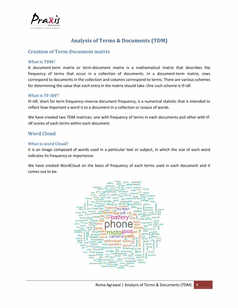
It is an image composed of words used in a particular text or subject, in which the size of each word

indicates its frequency or importance.

We have created WordCloud on the basis of frequency of each terms used in each document and it

comes out to be:


Words like “phone”, “battery”, “moto”, “good”, “camera” etc. got highlighted in this cloud. So we can

say that people have used these words too much in their statements. They have talked about camera,

battery, screen, display, means hardware specifications a lot. They have also talked about its

“performance”, “price”, “time”, “better” etc. which means they have expressed their views on the

performance of this phone. Word “flipkart” got highlighted, as this phone is only available on

www.flipkart.com hence they might have talked about the delivery process of flipkart. Rest words that

are displayed in smallest font size, are also important words but their frequency count is little less. From

these words we can say that people have compared this phone with similar Xiaomi and Samsung

products.

Dimension Reduction We have gone for dimension reduction i.e. Latent Semantic Analysis (LSA) using singular value

decomposition (SVD) because of following two reasons:

1. As there are 100 dimensions and 2282 terms, therefore, it will be difficult to analyze all these at

the same time.

2. TDM is essentially a very sparse matrix (99% sparseness is very common). So to remove

sparseness, LSA is used.

What are LSA and SVD?

Latent semantic analysis (LSA) is a technique in natural language processing, used for analyzing

relationships between a set of documents and the terms they contain by producing a set of concepts

related to the documents and terms. LSA assumes that words that are close in meaning will occur in

similar pieces of text. A matrix containing word counts per paragraph (rows represent unique words and

columns represent each paragraph) is constructed from a large piece of text and a mathematical

technique called singular value decomposition (SVD) is used to reduce the number of rows while

preserving the similarity structure among columns.

In simpler words, LSA gives a way of comparing documents at a higher level than the terms by

introducing a concept called the feature and SVD is a way of extracting features from documents.

The 3 matrices generated: Tk, Dk, Sk

The diagonal matrix Sk contains the singular values of TDM in descending order. The ith singular value

indicates the amount of variation along ith axis. Tk will consist of terms and values along each dimension.

Dk will consist of documents and its values along each dimension.

We can find the best approximated TDM by Tk*Sk*DkT.

For MOTO-G, we have found below three matrices and 50 dimensions after reduction.



Still, 50 dimensions are also too much for analysis, so we have chosen 3 dimensions to start with our

analysis work. As we can see, from matrix SK, dimensions V1, V2, V3 have highest singular value, which

means highest variation along these 3 dimensions, therefore selecting these 3 dimensions.

When terms were plotted against these 3 dimensions (using TK matrix), we got below graphs:

Above graph shows the positioning of each term in a 2 dimensional vector space. When we compare

two terms we compare the cosine of the angle between the vectors representing the terms. For

example, term “phone” is more towards the dimension V2 and “moto” is more towards dimension V1.


Similarly, this graph shows the placements of terms between V1 and V3 dimensions. with the help of

terms like “battery”, ”great”, ”games”, ”android” etc, we can say that dimension V1 constitutes the

specification of this phone, the features of this phone.

In this graph, cluster of words seems to be equally aligned with both the dimensions.


When documents were plotted against these 3 dimensions (using DK matrix), we got below graphs:

From these graph, we can say that the documents that are aligned more towards dimension V1, are

talking about the specifications of the phone. As we have seen that dimension V1 constitutes the terms

that talks about the features of this phone.

Documents 48, 49, 90, 99 etc. are aligned more towards dimension V2 than V1.


Similarly, for these two graphs.

Understanding the dimensions is a bit tough task. Therefore we tried to get some insights from TK and

DK matrix with the help of Cluster Analysis.

Clustering Cluster analysis or clustering is the task of grouping a set of objects in such a way that objects in the

same group (called a cluster) are more similar (in some sense or another) to each other than to those in

other groups (clusters).

We have done cluster analysis separately for both terms and documents after dimension reduction

(LSA).

Cluster Analysis for “Terms”

We have started with finding the optimal no of clusters using “hierarchical clustering” using ward

method. From below dendrogram, we got 4 options “3”, “5”, “6” and “7”. From these four options we

need to select one which will be the most optimal no of clusters. With the help of k-means clustering

and the size of clusters formed for each of above four options, we reached to the solution i.e. found “6”

to be the best case.


Below is the cluster plot, showing which terms belong to which cluster. Except cluster no 4, all are

overlapped. It is not very clear to infer anything from this plot.

Size for each cluster is:


To look into the clusters, we have created the WordCloud of each cluster which comes as below:

Now terms got cleared within each cluster.

Cluster1: This cluster seems to be comparison of MOTO-G’s features with phones like Xiaomi redmi and

Nexus on features like “touch”, ‘design”, “memory card slot”, “application updates” etc

Cluster2: This cluster purely tells about MOTO-G (2nd gen) phone, its specifications, its battery backup,

its performance, its availability on flipkart etc.

Cluster5: MOTO-G compared with Asus zenfone on hardware parts like “touch”, “buttons”, “colors”,

“models” etc.

Cluster3, cluster4, cluster6: nothing much can be inferred.

Cluster Analysis for “Documents”

For this also, we have started with finding the optimal no of clusters using “hierarchical clustering” using

ward method. From below dendrogram, we got 3 options “3”, “4” and “5”. From these three options we

need to select one which will be the most optimal no of clusters. With the help of k-means clustering

and the size of clusters formed for each of above options, we reached to the solution i.e. found “3” to be

the best case.


Below is the cluster plot, showing which document belongs to which cluster. For documents, the cluster

plot seems to be clear. It clearly shows which cluster comprises of which documents.

Size for each cluster is:

Roma Agrawal | Analysis of Ratings 13

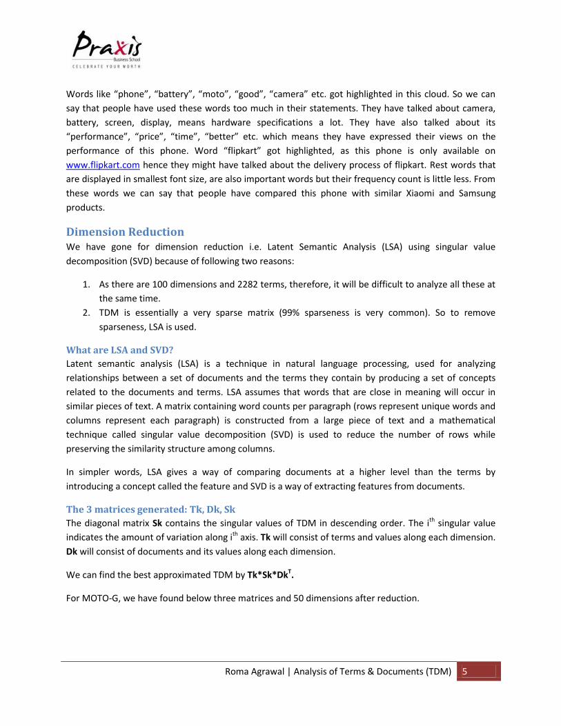
Analysis of Ratings

We have already extracted the ratings in the web crawling part. Now we need to classify customers of

MOTO-G into three categories:-

1. who are highly Impressed with this phone (ratings given = 4 and 5)

2. who are Satisfied with this phone (rating given = 3)

3. who are not at all satisfied (rating given = 1 and 2)

Note: on www.flipkart.com max rating is 5

Count of customers in each category is as follows:

More than 50% customers are Impressed with this phone, which is amazing news for the company.

However, company need to concentrate into 36% customers, their feedback, their views to know why

they are dissatisfied with this phone and they can work upon dissatisfied feedbacks to improve and

increase the satisfaction level among the customers.

Also, company can look into the “satisfied’ category people, how we can increase their satisfaction level

so that they change their perception and rate as “Impressed’ category customers.


Roma Agrawal | Importance of Terms on the basis of “Satisfaction” using SVM 14

Importance of Terms on the basis of “Satisfaction” using SVM

What is Classification? Classification is a data mining technique used to predict group membership for data instances. Following

are the examples of cases where the data analysis task is Classification:

A bank loan officer wants to analyze the data in order to know which customer (loan applicant)

is risky or which are safe.

A marketing manager at a company needs to analyze to guess a customer with a given profile

will buy a new computer.

In both of the above examples a model or classifier is constructed to predict categorical labels. These

labels are risky or safe for loan application data and yes or no for marketing data.

Similarly, here we will try to classify terms on the basis of satisfaction which will have two labels, two

categories:

1. Satisfied (rating given = 3, 4 and 5)

2. Dissatisfied (rating given = 1 and 2)

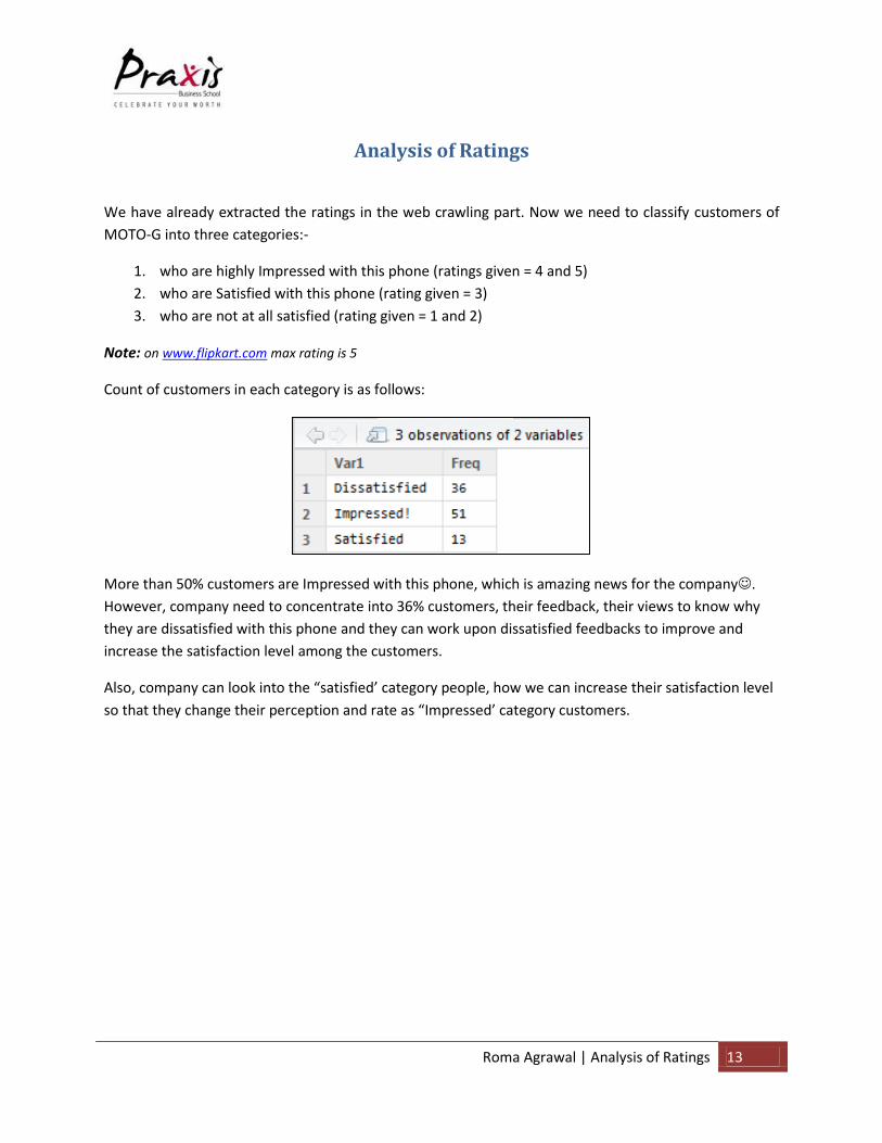
What is Support Vector Machine? A Support Vector Machine (SVM) is a discriminative classifier formally defined by a separating

hyperplane. In other words, given labeled training data (supervised learning), the algorithm outputs an

optimal hyperplane which categorizes new examples.

We have used SVM to do classification and to found the top most words which have highest weightage

for both negative and positive meaning.

Roma Agrawal | Sentiment Analysis 15

Sentiment Analysis

We have seen ratings given by customers. Let us now compare the reviews written and ratings given by

each customer. Let’s see many reviews matches with the ratings given.

What is sentiment analysis and polarity? Sentiment analysis aims to determine the attitude of a speaker or a writer with respect to some topic or

the overall contextual polarity of a document.

A basic task in sentiment analysis is classifying the polarity of a given text at the document, sentence, or

feature/aspect level — whether the expressed opinion in a document, a sentence or an entity

feature/aspect is positive, negative, or neutral. Advanced, "beyond polarity" sentiment classification

looks, for instance, at emotional states such as "angry," "sad," and "happy."

On the basis of polarity value (group stan.mean.polarity value), we have tried segregating the

customer’s review into three categories:

1. who are highly Impressed with this phone

2. who are Satisfied with this phone

3. who are not at all satisfied

But first, we need to find the threshold value of polarity:

Considering 0.1324276 as threshold, got below table:

This table seems to be matching with the counts that we have got from ratings. Here 54% customers

seem to be impressed by the use of MOTO-G. Most of the people have given ratings according to the

views that they have expressed.

Roma Agrawal | Appendix 16

Appendix

#web-crawling

init="http://www.flipkart.com/moto-g-2nd-gen/product

reviews/ITME3H4V4HKCFFCS?pid=MOBDYGZ6SHNB7RFC&type=top"

crawlcandidate="start="

base="http://www.flipkart.com"

num=10

doclist=list()

anchorlist=vector()

j=0

while(j<num){

if(j==0){

doclist[j+1]=getURL(init)

}else{

doclist[j+1]=getURL(paste(base,anchorlist[j+1],sep=""))

}

doc=htmlParse(doclist[[j+1]])

anchor=getNodeSet(doc,"//a")

anchor=sapply(anchor,function(x)xmlGetAttr(x,"href"))

anchor=anchor[grep(crawlcandidate,anchor)]

anchorlist=c(anchorlist,anchor)

anchorlist=unique(anchorlist)

j=j+1

}

#html_text is for extracting only reviews and ratings

reviews=c()

ratings=c()

for(i in 1:10){

doc=htmlParse(doclist[[i]])

l=getNodeSet(doc,"//div/p/span[@class='review-text']")

l1=html_text(l)

rateNodes=getNodeSet(doc,"//div[@class='fk-stars']")

rates=sapply(rateNodes,function(x)xmlGetAttr(x,'title'))

ratings=c(ratings,rates)

reviews=c(reviews,l1)

}

View(reviews)

View(ratings)

#saving files

save(reviews,file="F:\\Praxis\\Term3\\TextAnalytics\\Wordcloud\\MOTOG_Reviews.RData")

save(ratings,file="F:\\Praxis\\Term3\\TextAnalytics\\Wordcloud\\MOTOG_Ratings.RData")

#creating wordcloud

#tm,wordcloud

corpus=Corpus(VectorSource(reviews[1:100]))

corpus=tm_map(corpus,tolower)

corpus=tm_map(corpus,removePunctuation)

corpus=tm_map(corpus,removeNumbers)

corpus=tm_map(corpus,removeWords,stopwords("en"))

corpus=Corpus(VectorSource(corpus))

tdm=TermDocumentMatrix(corpus)

m=as.matrix(tdm)

v=sort(rowSums(m),decreasing=T)

d=data.frame(words=names(v),freq=v)

wordcloud(d$words,d$freq,max.words=300,colors=brewer.pal(10,"Dark2"),scale=c(3,0.5),random.order=

F)

#clearing existing data


remove(tdm)

remove(tdm_tfidf)

remove(m)

remove(m_tfidf)

remove(lsa_m)

remove(lsa_mtfidf)

remove(lsa_m_tk)

remove(lsa_mtfidf_tk)

remove(lsa_m_dk)

remove(lsa_mtfidf_dk)

#LSA using SVD

#rTextTools,lsa,tm

tdm=create_matrix(reviews,removeNumbers=T)

tdm_tfidf=weightTfIdf(tdm)

m=as.matrix(tdm)

m_tfidf=as.matrix(tdm_tfidf)

lsa_m=lsa(t(m),dimcalc_share(share=0.8))

lsa_m_tk=as.data.frame(lsa_m$tk)

lsa_m_dk=as.data.frame(lsa_m$dk)

lsa_m_sk=as.data.frame(lsa_m$sk)

#randomly creating 150 clusters with k-means

k150_m_tk=kmeans(scale(lsa_m_tk),centers=150,nstart=20)

c150_m_tk=aggregate(cbind(V1,V2,V3)~k150_m_tk$cluster,data=lsa_m_tk,FUN=mean)

k150_m_dk=kmeans(scale(lsa_m_dk),centers=50,nstart=20)

c150_m_dk=aggregate(cbind(V1,V2,V3)~k150_m_dk$cluster,data=lsa_m_dk,FUN=mean)

#hierarchical clustering to find optimal no of clusters for c150_m_tk

d=dist(scale(c150_m_tk[,-1]))

h=hclust(d,method='ward.D')

plot(h,hang=-1)

rect.hclust(h,h=20,border="blue")

rect.hclust(h,h=12,border="cyan")

rect.hclust(h,h=15,border="red")

#3,5,6

#6

k6_m_tk=kmeans(scale(lsa_m_tk),centers=6,nstart=20)

c6_m_tk=aggregate(cbind(V1,V2,V3)~k6_m_tk$cluster,data=lsa_m_tk,FUN=mean)

#hierarchical clustering to find optimal no of clusters for c150_m_dk

d=dist(scale(c150_m_dk[,-1]))

h=hclust(d,method='ward.D')

plot(h,hang=-1)

rect.hclust(h,h=5,border="blue")

rect.hclust(h,h=15,border="red")

rect.hclust(h,h=8,border="green")

#3,4,5

#3

k3_m_dk=kmeans(scale(lsa_m_dk),centers=3,nstart=20)

c3_m_dk=aggregate(cbind(V1,V2,V3)~k3_m_dk$cluster,data=lsa_m_dk,FUN=mean)

clusplot(lsa_m_dk, k3_m_dk$cluster, color=TRUE, shade=TRUE, labels=2, lines=0)

#Result of clustering on lsa_m_tk

v=sort(colSums(m),decreasing=T)

wordFreq=data.frame(words=names(v),freq=v)

k6_1_m_tk=wordFreq[k6_m_tk$cluster==1,]







wordcloud(k6_1_m_tk$words,k6_1_m_tk$freq,max.words=154,colors=brewer.pal(8,"Dark2"),scale=c(3,0.5

),random.order=F)

wordcloud(k6_2_m_tk$words,k6_2_m_tk$freq,max.words=300,colors=brewer.pal(8,"Dark2"),scale=c(3,0.5

),random.order=F)

wordcloud(k6_3_m_tk$words,k6_3_m_tk$freq,max.words=39,colors=brewer.pal(8,"Dark2"),scale=c(3,0.5)

,random.order=F)

wordcloud(k6_4_m_tk$words,k6_4_m_tk$freq,max.words=3,colors=brewer.pal(8,"Dark2"),scale=c(3,0.5),

random.order=F)


,random.order=F)


,random.order=F)

clusplot(lsa_m_tk, k6_m_tk$cluster, color=TRUE, shade=TRUE, labels=2, lines=0)

#lsa_m_tk

lsa_m_tk3=data.frame(words=rownames(lsa_m_tk),lsa_m_tk[,1:3])

plot(lsa_m_tk3$V1,lsa_m_tk3$V2)

text(lsa_m_tk3$V1,lsa_m_tk3$V2,label=lsa_m_tk3$words)





#Result of clustering on lsa_m_dk

lsa_m_dk=cbind(1:100,lsa_m_dk)

k3_1_m_dk=lsa_m_dk[k3_m_dk$cluster==1,]



colnames(lsa_m_dk)[1]="doc"

plot(lsa_m_dk$V1,lsa_m_dk$V2)

text(lsa_m_dk$V1,lsa_m_dk$V2,label=lsa_m_dk$doc)





#subset

#FSelector

lsa_m_tk6=cbind(lsa_m_tk,k6_m_tk$cluster)

names(lsa_m_tk6)[51]="cluster_tk"

lsa_m_tk6$cluster_tk=as.factor(lsa_m_tk6$cluster_tk)

subset_lsa_tk=cfs(cluster_tk~.,lsa_m_tk6)

f=as.simple.formula(subset_lsa_tk, "cluster_tk")

print(f)

lsa_m_dk3=cbind(lsa_m_dk,k3_m_dk$cluster)

names(lsa_m_dk3)[53]="cluster_dk"

lsa_m_dk3$cluster_dk=as.factor(lsa_m_dk3$cluster_dk)

subset_lsa_dk=cfs(cluster_dk~.,lsa_m_dk3)

f=as.simple.formula(subset_lsa_dk, "cluster")

print(f)

#Analysis of ratings

remove(finalratings)

finalratings=gsub(" stars","",ratings)

finalratings=gsub(" star","",finalratings)

View(finalratings)

finalratings1=as.numeric(finalratings)


satisfaction=ifelse(finalratings1<=2,"Dissatisfied",ifelse(finalratings1==3,"Satisfied","Impresse

d!"))

View(satisfaction)

#creating TDM with TF-IDF scores

dtm_MOTOG=create_matrix(reviews,removePunctuation=T,removeNumbers=T,weighting=weightTfIdf)

dtm_MOTOG=as.matrix(dtm_MOTOG)

data=as.data.frame(dtm_MOTOG)

data=cbind(data,satisfaction)

data$satisfaction

data1=cbind(1:100,data)

colnames(data1)[1]="doc"

count_satis=as.data.frame(table(data1$satisfaction))

#sentiments

#qdap

data2=data1

satisfaction1=as.data.frame(satisfaction)

for(i in 1:100)

{

sent=sent_detect(reviews[i])

pol=polarity(sent)

data2$polarity[i]=pol$group$stan.mean.polarity

satisfaction1$polarity_val[i]=pol$group$stan.mean.polarity

if(is.na(satisfaction1$polarity_val[i]))

{satisfaction1$polarity_val[i]=pol$group$ave.polarity

data2$polarity[i]=pol$group$ave.polarity}

}

new_rate=cbind(finalratings1,satisfaction1)

aggregate(polarity_val~finalratings1,data=new_rate,FUN=mean)

new_rate$status=ifelse(new_rate$polarity_val>0.1324276,"Impressed!",ifelse(new_rate$polarity_val<

=-0.4982026,"Dissatisfied","Satisfied"))

count_status1=as.data.frame(table(new_rate$status))

View(count_satis)

View(count_status1)

#Classification condidering two levels for satisfaction "Satisfied" >=3

View(data)

data3=data[1:2282]

satis=ifelse(finalratings1>2,"satisfied","dissatisfied")

data3=cbind(data3,satis)

data3=na.omit(data3)

data3=data3[,colSums(data3[,-length(data3)])>0]

svm=svm(satis~.,data=data3)

coef_imp=as.data.frame(t(svm$coefs)%*%svm$SV)

coef_imp1=data.frame(words=names(coef_imp),Importance=t(coef_imp))

coef_imp1=coef_imp1[order(coef_imp1$Importance),]

head(coef_imp1)

tail(coef_imp1)

Roma Agrawal | Bibliography 20

Bibliography

1. http://oak.cs.ucla.edu/~cho/research/crawl.html

2. http://en.wikipedia.org/wiki/Main_Page

3. http://www.tutorialspoint.com/data_mining/dm_classification_prediction.htm

4. https://docs.google.com/presentation/d/1iDtcXITpWwg9RMzVvdOOiJ1IJBLvbyeLrzBGXdDLTVA/

edit?usp=sharing

http://oak.cs.ucla.edu/~cho/research/crawl.html

http://en.wikipedia.org/wiki/Main_Page

http://www.tutorialspoint.com/data_mining/dm_classification_prediction.htm

https://docs.google.com/presentation/d/1iDtcXITpWwg9RMzVvdOOiJ1IJBLvbyeLrzBGXdDLTVA/edit?usp=sharing

https://docs.google.com/presentation/d/1iDtcXITpWwg9RMzVvdOOiJ1IJBLvbyeLrzBGXdDLTVA/edit?usp=sharing

Data & Analytics

Text Analysis Report