Tall-and-skinny Matrix Computations in MapReduce (ICME colloquium)

Tall-and-skinny Matrix Computations inMapReduce

Austin Benson

Institute for Computational and Mathematical EngineeringStanford University

ICME Colloquium

May 20, 2013

Collaborators 2

James Demmel, UC-Berkeley David Gleich, Purdue

Paul Constantine, Stanford

Thanks!

Matrices and MapReduce 3

Matrices and MapReduce

Warm-up: Ax

|| · ||

ATA

QR and SVD

MapReduce overview 4

Two functions that operate on key value pairs:

(key , value)map−−→ (key , value)

(key , 〈value1, . . . , valuen〉)reduce−−−−→ (key , value)

A shuffle stage runs between map and reduce to sort the values bykey.


Scalability: many map tasks and many reduce tasks are used

https://developers.google.com/appengine/docs/python/images/mapreduce_mapshuffle.png

https://developers.google.com/appengine/docs/python/images/mapreduce_mapshuffle.png


The idea is data-local computations. The programmer implements:

I map(key, value)

I reduce(key, 〈 value1, . . ., valuen 〉)

The shuffle and data I/O is implemented by the MapReduceframework, e.g., Hadoop.

MapReduce Example: ColorCount 7

(key, value) input is (image id, image)

1 1 1 1 1 1 1 1

1 1 1 1 1 1 1 1

shuffle

1

1

1

1

1

1

1

1

1

1

1

1 1

1

1

1 Map Reduce

1

5

2

1

1

4 2

def ColorCountMap(key , val ) :for pixel in val :

yield ( pixel , 1)

def ColorCountReduce(key , vals ) :total = sum( vals )yield (key , total )

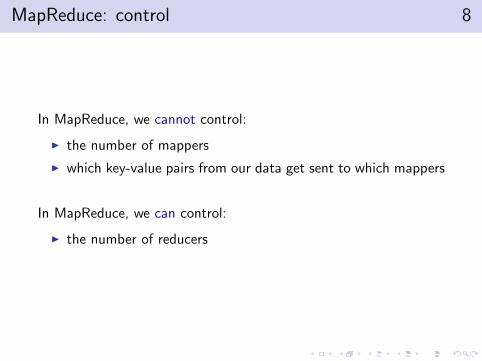
MapReduce: control 8

In MapReduce, we cannot control:

I the number of mappers

I which key-value pairs from our data get sent to which mappers

In MapReduce, we can control:

I the number of reducers

Why MapReduce? 9

MapReduce is a very restrictive programming environment! Whybother?

1. Fault tolerance

2. Structured data I/O

3. Cheaper clusters with more data storage

4. Easy to program

Generate lots of data on supercomputer

Post-process and analyze on MapReduce cluster

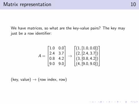
Matrix representation 10

We have matrices, so what are the key-value pairs? The key mayjust be a row identifier:

A =

1.0 0.02.4 3.70.8 4.29.0 9.0

→

(1, [1.0, 0.0])(2, [2.4, 3.7])(3, [0.8, 4.2])(4, [9.0, 9.0])

(key, value) → (row index, row)

Matrix representation 11

Maybe the data is a set of samples

A =

1.0 0.02.4 3.70.8 4.29.0 9.0

→

(“Apr 26 04:18:49”, [1.0, 0.0])(“Apr 26 04:18:52”, [2.4, 3.7])(“Apr 26 04:19:12”, [0.8, 4.2])(“Apr 26 04:22:33”, [9.0, 9.0])

(key, value) → (timestamp, sample)

Matrix representation: an example 12

Scientific example: (x, y, z) coordinates and model number:

((47570,103.429767811242,0,-16.525510963787,iDV7), [0.00019924

-4.706066e-05 2.875293979e-05 2.456653e-05 -8.436627e-06 -1.508808e-05

3.731976e-06 -1.048795e-05 5.229153e-06 6.323812e-06])

Figure: Aircraft simulation data. Paul Constantine, Stanford University

Tall-and-skinny matrices 13

What are tall-and-skinny matrices?

A m

n

A is m × n and m >> n. Examples: rows are data samples; blocksof A are images from a video; Krylov subspaces; Unrolled tensors

Warm-up: Ax 14


Warm-up: Ax

|| · ||

ATA

QR and SVD

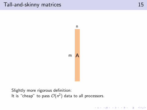
Tall-and-skinny matrices 15

A m

n

Slightly more rigorous definition:It is “cheap” to pass O(n2) data to all processors.

Ax : Local to Distributed 16

A

X’

A1

X’

A2

X’

A3

X’

A4

X’

A5

X’

A6

X’

Ax : distributed store, distributed computation 17

A may be stored in an uneven, distributed fashion. TheMapReduce framework provides load balance.

A1

X’

A2

X’

A3

X’

A4

X’

A5

X’

A6

X’

A1

A2

A3

Ax : MapReduce perspective 18

The programmer’s perspective for map():

A? map

X’ (A?)i Output data

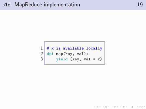
Ax : MapReduce implementation 19

1 # x is available locally

2 def map(key, val):

3 yield (key, val * x)

Ax : MapReduce implementation 20

I We didn’t even need reduce!

I The output is stored in distributed fashion:

(Ax)1 (Ax)2

(Ax)3 (Ax)4

(Ax)5 (Ax)6

|| · || 21


Warm-up: Ax

|| · ||

ATA

QR and SVD

||Ax || 22

I Global information → need reduce

I Examples: ||Ax ||1, ||Ax ||2, ||Ax ||∞, |Ax |0

||y ||22 23

Assume we have already computed y = Ax .

y1 y2

y3 y4

y5 y6

||y ||22 24

What can we do with a partial partition of y?

map y?

(y?)i

||y ||22 map 25

We could just compute the squares of each


2 yield (0, val * val)

... then we need to sum the squares

||y ||22 map and reduce 26

Only one key → everything sent to a single reducer.


2 # only one key


45 def reduce(key, vals):

6 yield (’norm2’, sum(vals))

||y ||22 map and reduce 27

How can this be improved?


2 # only one key




||y ||22 improvement 28

Idea: use more reducers

1 def map1(key , val ) :2 key = uniform random([1 , 2 , 3 , 4 , 5 , 6])3 yield (key , val ∗ val )45 def reduce1(key , vals ) :6 yield (key , sum( vals ))78 def map2(key , val ) :9 yield (0 , val )

1011 def reduce2(key , vals ) :12 yield ( ’norm2 ’ , sum( vals ))

map1() → reduce1() → map2() → reduce2()


y1 y2

y3 y4

y5 y6

yT2y2 yT

1y1

yT4y4 yT

3y3

yT6y6 yT

5y5

yT2y2 yT

1y1

yT4y4 yT

3y3

yT6y6 yT

5y5

yT1y1 + … + yT

6y6

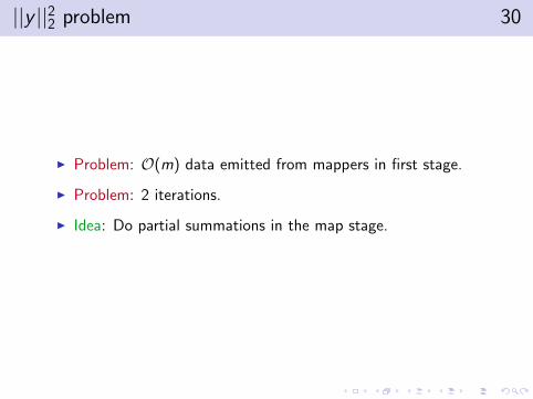
||y ||22 problem 30

I Problem: O(m) data emitted from mappers in first stage.

I Problem: 2 iterations.

I Idea: Do partial summations in the map stage.


1 partial_sum_sq = 0


3 partial_sum += val * val

4 if key == last_key:

5 yield (0, partial_sum)



I This is the idea of a combiner.

I O(#(mappers)) data emitted from mappers.

||Ax ||22 32

I Suppose we only care about ||Ax ||22, not y = Ax and ||y ||22.

I Can we do better than:

(1) compute y = Ax(2) compute ||y ||22

?

I Of course!

||Ax ||22 33

Combine our previous ideas:


2 yield (0, (val * x) * (val * x))


5 yield sum(vals)

Other norms 34

I We can easily extend these ideas to other norms

I Basic idea for computing ||y ||:

(1) perform some independent operation on each yi(2) combine the results

||Ax || and |Ax |0 35

def map abs(key , val ) :yield (0 , | value ∗ x |)

def map square(key , val ) :yield (0 , (value ∗ x)ˆ2)

def map zero(key , val ) :i f val ∗ x == 0:yield (0 , 1)

def reduce sum(key , vals ) :yield sum( vals )

def reduce max(key , vals ) :yield max( vals )

I ||Ax ||1: map abs() → reduce sum()

I ||Ax ||22: map square() → reduce sum()

I ||Ax ||∞: map abs() → reduce max()

I |Ax |0: map zero() → reduce sum()

ATA 36


Warm-up: Ax

|| · ||

ATA

QR and SVD

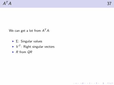
ATA 37

We can get a lot from ATA:

I Σ: Singular values

I V T : Right singular vectors

I R from QR

ATA 38

We can get a lot from ATA:

I Σ: Singular values

I V T : Right singular vectors

I R from QR

with a little more work...

I U: Left singular vectors

I Q from QR

ATA: MapReduce 39

I Computing ATA is similar to computing ||y ||22.

I Idea: ATA =m∑i=1

aTi ai (ai is the i-th row).

I → Sum of m n × n rank-1 matrices.


2 # .T --> Python NumPy transpose

3 yield (0, val.T * val)


6 yield (0, sum(vals))

ATA: MapReduce 40

A1 A2

A3 A4

A5 A6

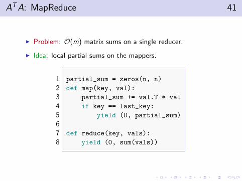
ATA: MapReduce 41

I Problem: O(m) matrix sums on a single reducer.

I Idea: local partial sums on the mappers.

1 partial_sum = zeros(n, n)


3 partial_sum += val.T * val

4 if key == last_key:

5 yield (0, partial_sum)


8 yield (0, sum(vals))

ATA: MapReduce 42

A1 A2

A3 A4

A5 A6

I O(#(mappers)) matrix sums on a single reducer

QR and SVD 43


Warm-up: Ax

|| · ||

ATA

QR and SVD

Quick QR and SVD review 44

A Q R

VT

n

n

n

n

n

n

A U n

n

n

n

n

n

Σ

n

n

Figure: Q, U, and V are orthogonal matrices. R is upper triangular andΣ is diagonal with nonnegative entries.

Quals / 45

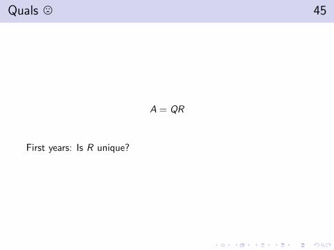
A = QR

First years: Is R unique?

Tall-and-skinny QR 46

A Q

R

m

n

m

n n

n

Tall-and-skinny (TS): m >> n. QTQ = I .

TS-QR → TS-SVD 47

A Q

R Σ VT

Q

UR

U

R is small, so computing its SVD is cheap.

Why Tall-and-skinny QR and SVD? 48

1. Regression with many samples

2. Principle Component Analysis (PCA)

3. Model Reduction

Pressure, Dilation, Jet Engine

Figure: Dynamic mode decomposition of the screech of a jet. JoeNichols, Stanford University.

Cholesky QR 49

Cholesky QR

ATA = (QR)T (QR) = RTQTQR = RTR

I We already saw how to compute ATA.

I Compute R = Cholesky(ATA) locally (cheap)

Stability problems 50

I Problem: ATA→ square the condition number

I Idea: Use a more advanced algorithm

Communication-avoiding TSQR 51

A =

A1

A2

A3

A4

︸︷︷︸8n×4n

=

Q1

Q2

Q3

Q4

︸︷︷︸

8n×4n

R1

R2

R3

R4

︸︷︷︸4n×n

=

=Q︷︸︸︷Q1

Q2

Q3

Q4

︸︷︷︸

8n×4n

Q̃︸︷︷︸4n×n

R︸︷︷︸n×n

Demmel et al. 2008


A =

A1

A2

A3

A4

︸︷︷︸8n×4n

=

Q1

Q2

Q3

Q4

︸︷︷︸

8n×4n

R1

R2

R3

R4

︸︷︷︸4n×n

Ai = QiRi can be computed in parallel. If we only need R, thenwe can throw out the intermediate Qi factors.

Mapper’s perspective 53

I A given map task computes QR of its data.

I Idea: gather rows until QR computation just fits in cache

[A1i

] QR−−→[R] read A1

i−−−−→[

RA1i

]QR−−→

[R] read A2

i−−−−→[

RA2i

]QR−−→

[R]

. . .read AN

i−−−−−→[

RANi

]QR−−→

[R] emit−−→

Aji are groups of rows of Ai that are read by i-th mapper

MapReduce TSQR 54

S(1)

A

A1

A2

A3

A3

R1 map

A2

emit R2 map

A3

emit R3 map

A4

emit R4 map

shuffle

S1

A2

reduce

S2 R2,2

reduce

R2,1 emit

emit

emit

shuffle

A2 S3 R2,3

reduce emit

Local TSQR

identity map

A2 S(2) R reduce emit

Local TSQR Local TSQR

Figure: S (1) is the matrix consisting of the rows of all of the Ri factors.Similarly, S (2) consists of all of the rows of the R2,j factors.

MapReduce TSQR: the implementation 55

1 import random, numpy, hadoopy2 class SerialTSQR:3 def i n i t ( self , blocksize , isreducer ) :4 se l f . bsize , se l f . data =blocksize , [ ]5 se l f . c a l l = se l f . reducer i f isreducer else se l f .mapper67 def compress( se l f ) :8 R = numpy. l ina lg . qr(numpy. array( se l f . data) , ’ r ’ )9 se l f . data = [ [ f loat (v) for v in row] for row in R]

1011 def col lect ( self , key , value ) :12 se l f . data .append(value)13 i f len ( se l f . data) > se l f . bsize ∗ len ( se l f . data [0 ] ) :14 se l f . compress()1516 def close ( se l f ) :17 se l f . compress()18 for row in se l f . data : yield random. randint(0,2000000000), row1920 def mapper( self , key , value ) :21 se l f . co l lect (key , value)2223 def reducer( self , key , values ) :24 for value in values : se l f .mapper(key , value)2526 i f name ==’ main ’ :27 mapper = SerialTSQR(blocksize=3, isreducer=False)28 reducer = SerialTSQR(blocksize=3, isreducer=True)29 hadoopy. run(mapper, reducer)

MapReduce TSQR: Getting Q 56

We have an efficient way of getting R in QR (and Σ in the SVD).What if I want Q (or my left singular vectors)?

A = QR → Q = AR−1

(just a backsolve). Problem: Q can be far from orthogonal. (Thismay be OK in some cases).

Indirect TSQR 57

We call this method Indirect TSQR.

A

A1 R-1 map

R

Q1

A2 R-1 map

Q2

A3 R-1 map

Q3

A4 R-1 map

Q4

emit

emit

emit

emit

distribute

Local MatMul

Indirect TSQR: Iterative Refinement 58

We can repeat the TSQR computation on Q to get a moreorthogonal matrix. This is called iterative refinement.

A

A1 R-1 map

R

Q1

A2 R-1 map

Q2

A3 R-1 map

Q3

A4 R-1 map

Q4

emit

emit

emit

emit

distribute

TSQ

R

Q

Q1 R1

-1 map

R1

Q1

Q2 R1

-1 map

Q2

Q3 R1

-1 map

Q3

Q4 R1

-1 map

Q4

emit

emit

emit

emit

distribute

Local MatMul Local MatMul

Iterative Refinement step

Indirect TSQR: a randomized approach 59

I Idea: Take a small sample of rows of A and form Rs

I Refinement step by Qs = AR−1s , Qs → R1, Q = QsR−11

I R = R1Rs , QTQ ≈ I for ill-conditioned A

I Some theory on why this works[Mahoney 2011], [Avron, Maymounkov, and Toledo 2010]

We call this Pseudo-Iterative Refinement

Pseudo-Iterative Refinement 60

A

A1 Rs

-1 map

Rs

Q1

A2 Rs

-1 map

Q2

A3 Rs

-1 map

Q3

A4 Rs

-1 map

Q4

emit

emit

emit

emit

distribute

TSQ

R

Q

Q1 R1

-1 map

R1

Q1

Q2 R1

-1 map

Q2

Q3 R1

-1 map

Q3

Q4 R1

-1 map

Q4

emit

emit

emit

emit

distribute

Local MatMul Local MatMul

Iterative Refinement step Form Qs

A1

TSQ

R

Form Rs

(In the implementation, combine AR−1s and TSQR in one pass)

Direct TSQR 61

Why is it hard to reconstruct an orthogonal Q directly?

I Orthogonality is a global property, but we compute locally.

I No controlled communication between processors → can onlycontrol data movement via the shuffle.

I Can only label data via keys and file names.


A =

A1

A2

A3

A4

︸︷︷︸8n×4n

=

Q1

Q2

Q3

Q4

︸︷︷︸

8n×4n

R1

R2

R3

R4

︸︷︷︸4n×n

=

Q1

Q2

Q3

Q4

︸︷︷︸

8n×4n

Q2

1

Q22

Q23

Q24

︸︷︷︸4n×n

R︸︷︷︸n×n

=

Q1Q

21

Q2Q22

Q3Q21

Q4Q21

︸︷︷︸

8n×n

R︸︷︷︸n×n

= QR

Gathering Q 63

R1

R2

R3

R4

︸︷︷︸

n·#(mappers)×n

=

Q2

1

Q22

Q23

Q24

︸︷︷︸

n·#(mappers)×n

R︸︷︷︸n×n

I Idea: Can compute QR of n ·#(mappers)× n matrix on asingle CPU

I Idea: Can pass Q2i of size n × n in a second pass to

reconstruct Q of A

I We call this Direct TSQR

Direct TSQR: Steps 1 and 2 64

A

A1 R1 map

emit Q11 emit

A2 R2 map

emit Q21

emit

A3 R3 map

emit Q31

emit

A4 R4 map

emit Q41

emit

First step

R1

R2

R3

R4

Q12

Q22

Q32

Q42

R

reduce

emit

emit

emit

emit

emit

Second step

shuffle

Direct TSQR: Step 3 65

Q11 Q12

emit Q1 map

Q21 Q22

emit Q2 map

Q31 Q32

emit Q3 map

Q41 Q42

emit Q4 map

Q12 Q22

Q32 Q42 distribute

Third step

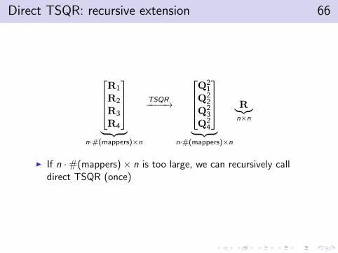
Direct TSQR: recursive extension 66

R1

R2

R3

R4

︸︷︷︸

n·#(mappers)×n

TSQR−−−−→

Q2

1

Q22

Q23

Q24

︸︷︷︸

n·#(mappers)×n

R︸︷︷︸n×n

I If n ·#(mappers)× n is too large, we can recursively calldirect TSQR (once)

Scaling columns 67

I Scaling to more columns is difficult: key-value pairs becomelarge → more communication

I Sampling approaches:[Zadeh and Goel 2012] [Zadeh and Carlsson 2013]

I Panel factorization

Direct TSQR: recursive performance 68

0 50 100 150 200 250 3000

2000

4000

6000

8000

10000

12000

tim

e t

o c

om

ple

tio

n (

s)

number of columns

Column scaling Direct TSQR

no recursion (150M)

recursion (150M)

no recursion (100M)

recursion (100M)

no recursion (50M)

recursion (50M)

0 50 100 150 200 250 3000

100

200

300

400

500

600

700

800

number of columns

siz

e (

KB

)

(key, value) pair size in Direct MRTSQR step II

approx. (key, value) pair

L1 cache

L2 cache

Stability 69

100

102

104

106

108

1010

1012

1014

1016

10−16

10−14

10−12

10−10

10−8

10−6

10−4

10−2

100

102

κ2(A)

||Q

TQ

− I

||2

Numerical stability: 10000x10 matrices

Pseudo−I.R.

Dir. TSQR

Indir. TSQR

Indir. TSQR + I.R.

Chol.

Chol. + I.R.

Overall Performance 70

4B x 4(134.6 GB)

2.5B x 10(193.1 GB)

600M x 25(112.0 GB)

500M x 50(183.6 GB)

150M x 100(109 GB)

Matrix size

0

1000

2000

3000

4000

5000

6000

7000

8000Tim

e t

o s

olu

tion (

seco

nds)

Performance of QR algorithms on MapReduce

Chol.

Indir. TSQR

Chol. + I.R.

Indir. TSQR + I.R.

Pseudo-I.R.

Dir. TSQR

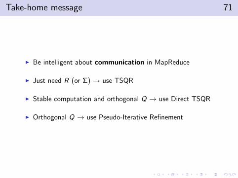
Take-home message 71

I Be intelligent about communication in MapReduce

I Just need R (or Σ) → use TSQR

I Stable computation and orthogonal Q → use Direct TSQR

I Orthogonal Q → use Pseudo-Iterative Refinement

Questions 72

Questions?

I [email protected]

I Code: https://github.com/arbenson/mrtsqr

https://github.com/arbenson/mrtsqr

Data & Analytics

Tall-and-skinny Matrix Computations in MapReduce (ICME colloquium)