Recommendation SystemArchit GuptaSeptember 6, 2016Recommendation systems, also referred to as recommender systems, often rely on the notion of similarity between objects, in anapproach known as collaborative filtering. Its basic premise is that customers can be considered similar to each other if they share most ofthe products that they have purchased; equally, items can be considered similar to each other if they share a large number of customerswho purchased them.

There are a number of different ways to quantify this notion of similarity, and we will present some of the commonly used alternatives.Whether we want to recommend movies, books, hotels, or restaurants, building a recommender system often involves dealing with verylarge data sets.

Rating matrixA recommendation system usually involves having a set of users U = {u1, u2, ., um} that have varying preferences on a set of items I ={i1, i2, ., in}. The number of users |U| = m is different from the number of items |I| = n in the general case. In addition, users can oftenexpress their preference by rating items on some scale. As an example, we can think of the users as being restaurant patrons in a city,and the items being the restaurants that they visit. Under this setup, the preferences of the users could be expressed as ratings on a fivestar scale. Of course, our generalization does not require that the items be physical items or that the users be actual people-this is simplyan abstraction for the recommender system problem that is commonly used.

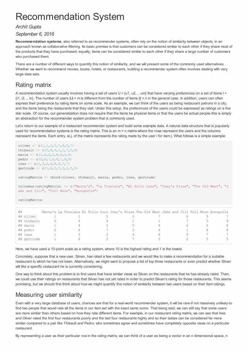
Let’s return to our example of a restaurant recommender system and build some example data. A natural data structure that is popularlyused for recommendation systems is the rating matrix. This is an m × n matrix where the rows represent the users and the columnsrepresent the items. Each entry, ei,j, of the matrix represents the rating made by the user i for item j. What follows is a simple example:

oliver <- c(1,1,2,5,7,8,9,7)thibault <- c(5,9,4,1,1,7,5,9)maria <- c(1,4,2,5,8,6,2,8)pedro <- c(2,6,7,2,6,1,8,9)ines <- c(1,3,2,4,8,9,7,7)gertrude <- c(1,6,5,7,3,2,5,5)

ratingMatrix <- rbind(oliver, thibault, maria, pedro, ines, gertrude)

colnames(ratingMatrix) <- c("Berny's", "La Traviata", "El Pollo Loco", "Joey's Pizza", "The Old West", "Jake and Jill", "Full Moon", "Acropolis")

ratingMatrix

## Berny's La Traviata El Pollo Loco Joey's Pizza The Old West Jake and Jill Full Moon Acropolis## oliver 1 1 2 5 7 8 9 7## thibault 5 9 4 1 1 7 5 9## maria 1 4 2 5 8 6 2 8## pedro 2 6 7 2 6 1 8 9## ines 1 3 2 4 8 9 7 7## gertrude 1 6 5 7 3 2 5 5

Here, we have used a 10-point scale as a rating system, where 10 is the highest rating and 1 is the lowest.

Concretely, suppose that a new user, Silvan, has rated a few restaurants and we would like to make a recommendation for a suitablerestaurant to which he has not been. Alternatively, we might want to propose a list of top three restaurants or even predict whether Silvanwill like a specific restaurant he is currently considering.

One way to think about this problem is to find users that have similar views as Silvan on the restaurants that he has already rated. Then,we could use their ratings on restaurants that Silvan has not yet rated in order to predict Silvan’s rating for those restaurants. This seemspromising, but we should first think about how we might quantify this notion of similarity between two users based on their item ratings.

Measuring user similarityEven with a very large database of users, chances are that for a real-world recommender system, it will be rare-if not massively unlikely-tofind two people that would rate all the items in our item set with the exact same score. That being said, we can still say that some usersare more similar than others based on how they rate different items. For example, in our restaurant rating matrix, we can see that Inesand Oliver rated the first four restaurants poorly and the last four restaurants highly and so their tastes can be considered far moresimilar compared to a pair like Thibault and Pedro, who sometimes agree and sometimes have completely opposite views on a particularrestaurant.

By representing a user as their particular row in the rating matrix, we can think of a user as being a vector in an n dimensional space, n

being the number of items. Thus we can use different distance measures appropriate for vectors in order to measure the similarity of twodifferent users. Note that the notion of distance is inversely proportional to the notion of similarity and we can thus use measures ofdistance as measures of similarity by interpreting a large distance between two vectors as analogous to a low similarity score.

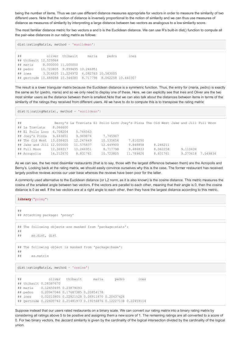
The most familiar distance metric for two vectors a and b is the Euclidean distance. We can use R’s built-in dist() function to compute allthe pair-wise distances in our rating matrix as follows:

dist(ratingMatrix, method = 'euclidean')

## oliver thibault maria pedro ines## thibault 12.529964 ## maria 8.000000 11.000000 ## pedro 10.723805 9.899495 10.246951 ## ines 3.316625 11.224972 6.082763 10.583005 ## gertrude 10.488088 10.344080 8.717798 8.062258 10.440307

The result is a lower triangular matrix because the Euclidean distance is a symmetric function. Thus, the entry for (maria, pedro) is exactlythe same as for (pedro, maria) and so we only need to display one of these. Here, we can explicitly see that Ines and Oliver are the twomost similar users as the distance between them is smallest.Note that we can also talk about the distances between items in terms of thesimilarity of the ratings they received from different users. All we have to do to compute this is to transpose the rating matrix:

dist(t(ratingMatrix), method = 'euclidean')

## Berny's La Traviata El Pollo Loco Joey's Pizza The Old West Jake and Jill Full Moon## La Traviata 8.366600 ## El Pollo Loco 6.708204 5.744563 ## Joey's Pizza 9.643651 9.949874 7.745967 ## The Old West 13.038405 12.247449 10.535654 7.810250 ## Jake and Jill 12.000000 11.575837 12.449900 9.848858 8.246211 ## Full Moon 12.369317 10.246951 8.717798 9.486833 8.062258 9.110434 ## Acropolis 14.212670 8.831761 10.723805 11.789826 8.831761 9.273618 7.549834

As we can see, the two most dissimilar restaurants (that is to say, those with the largest difference between them) are the Acropolis andBerny’s. Looking back at the rating matrix, we should easily convince ourselves why this is the case. The former restaurant has receivedlargely positive reviews across our user base whereas the reviews have been poor for the latter.

A commonly used alternative to the Euclidean distance (or L2 norm, as it is also known) is the cosine distance. This metric measures thecosine of the smallest angle between two vectors. If the vectors are parallel to each other, meaning that their angle is 0, then the cosinedistance is 0 as well. If the two vectors are at a right angle to each other, then they have the largest distance according to this metric.

library("proxy")

## ## Attaching package: 'proxy'

## The following objects are masked from 'package:stats':## ## as.dist, dist

## The following object is masked from 'package:base':## ## as.matrix

dist(ratingMatrix, method = 'cosine')

## oliver thibault maria pedro ines## thibault 0.28387670 ## maria 0.12450495 0.23879093 ## pedro 0.20947046 0.17687385 0.20854178 ## ines 0.02010805 0.22821528 0.06911870 0.20437426 ## gertrude 0.22600742 0.21481973 0.19156876 0.12227138 0.22459114

Suppose instead that our users rated restaurants on a binary scale. We can convert our rating matrix into a binary rating matrix byconsidering all ratings above 5 to be positive and assigning them a new score of 1. The remaining ratings are all converted to a score of0. For two binary vectors, the Jaccard similarity is given by the cardinality of the logical intersection divided by the cardinality of the logicalunion.

binaryRatingMatrix <- ratingMatrix > 5dist(binaryRatingMatrix, method = 'jaccard')

## oliver thibault maria pedro ines## thibault 0.6000000 ## maria 0.2500000 0.5000000 ## pedro 0.5000000 0.6666667 0.6666667 ## ines 0.0000000 0.6000000 0.2500000 0.5000000 ## gertrude 1.0000000 0.7500000 1.0000000 0.8333333 1.0000000

Collaborative filteringcollaborative filtering, will help us define a strategy for making recommendations. Collaborative filtering describes an algorithm, or moreprecisely a family of algorithms, that aims to create recommendations for a test user given only information about the ratings of otherusers via the rating matrix, as well as any ratings that the test user has already made.

There are two very common variants of collaborative filtering, memory-based collaborative filtering and model-based collaborativefiltering. With memory-based collaborative filtering, the entire history of all the ratings made by all the users is remembered and must beprocessed in order to make a recommendation. The prototypical memory-based collaborative filtering method is user-based collaborativefiltering. Although this approach uses all the ratings available, the downside is that it can be computationally expensive as the entiredatabase is used in order to make rating predictions for our test user.

The alternative approach to this is embodied in model-based collaborative filtering. Here, we first create a model of the rating preferencesof our users, such as a set of clusters of users who like similar items, and then use the model to generate recommendations. We will studyitem-based collaborative filtering, which is the most well-known model-based collaborative filtering method.

User-based collaborative filteringUser-based collaborative filtering is commonly described as a memory-based or lazy learning approach.in user-based collaborativefiltering, when we want to make recommendations for a new user, we will first pick a set of similar users using a particular distance metric.Then, we try to infer the ratings that our target user would assign to items that he or she has not yet rated as an average of the ratingsmade by these similar users on those items. We usually refer to this set of similar users as the user’s neighborhood. Thus, the idea is thata user will prefer items that their neighborhood prefers.

Typically, there are two ways to define the user’s neighborhood. We can compute a fixed neighborhood by finding the k-nearestneighbors. These are the k users in our database that have the smallest distance between them and our target user.

Alternatively, we can specify a similarity threshold and pick all the users in our database whose distance from our target user does notexceed this threshold. This second approach has the advantage that we will be making recommendations using users that are as close toour target user as we want, and therefore our confidence in our recommendation can be high. On the other hand, there might be very fewusers that satisfy our requirement, meaning that we will be relying on the recommendations of these few users. Worse, there might be nousers in our database who are sufficiently similar to our target user and we might not be able to actually make a recommendation at all. Ifwe don’t mind our method sometimes failing to make a recommendation, for example because we have a backup plan to handle thesecases, the second approach might be a good choice.

Another important consideration to make in a real-world setting is the problem of sparse ratings. In our simple restaurant example, everyuser had rated every restaurant. This rarely happens in a real situation, if ever, simply because the number of items is usually too big fora user to rate them all. If we think of e-commerce websites such as amazon.com, for example, it is easy to imagine that the most productsthat any user has rated is still only a small fraction of the overall number of products on sale.

Once we have decided on a distance metric and how to form a neighborhood of users that are similar to our test user, we then use thisneighborhood to compute the missing ratings for the test user. The easiest way to do this is to simply compute the average rating foreach item in the user neighborhood and report this value.

A first possible improvement comes from the observation that some users will tend to consistently rate items more strictly or more lenientlythan other users, and we would like to smooth out this variation. In practice, we often use Z-score normalization, which takes into accountthe variance of the ratings. We can also center each rating made by a user by subtracting that user’s average rating across all the items.In the rating matrix, this means subtracting the mean of each row from the elements of the row. Let’s apply this last transformation to ourrestaurant rating matrix and see the results:

centered_rm <- t(apply(ratingMatrix, 1, function(x) x - mean(x)))centered_rm

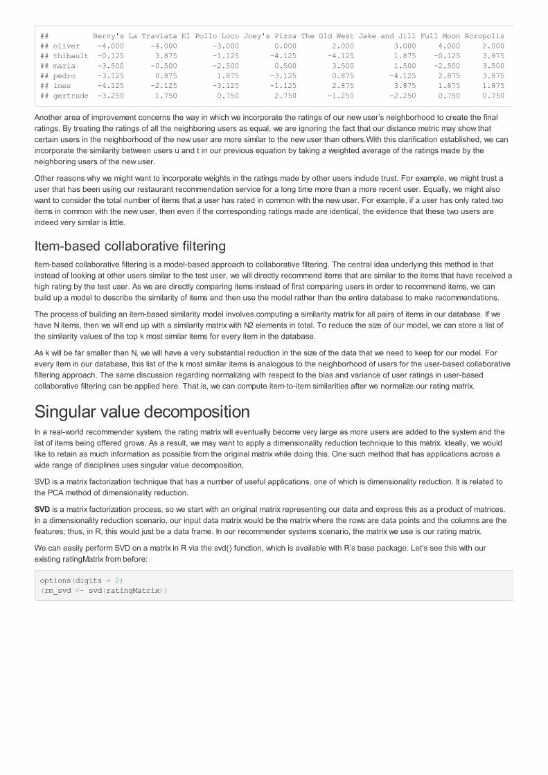
## Berny's La Traviata El Pollo Loco Joey's Pizza The Old West Jake and Jill Full Moon Acropolis## oliver -4.000 -4.000 -3.000 0.000 2.000 3.000 4.000 2.000## thibault -0.125 3.875 -1.125 -4.125 -4.125 1.875 -0.125 3.875## maria -3.500 -0.500 -2.500 0.500 3.500 1.500 -2.500 3.500## pedro -3.125 0.875 1.875 -3.125 0.875 -4.125 2.875 3.875## ines -4.125 -2.125 -3.125 -1.125 2.875 3.875 1.875 1.875## gertrude -3.250 1.750 0.750 2.750 -1.250 -2.250 0.750 0.750

Another area of improvement concerns the way in which we incorporate the ratings of our new user’s neighborhood to create the finalratings. By treating the ratings of all the neighboring users as equal, we are ignoring the fact that our distance metric may show thatcertain users in the neighborhood of the new user are more similar to the new user than others.With this clarification established, we canincorporate the similarity between users u and t in our previous equation by taking a weighted average of the ratings made by theneighboring users of the new user.

Other reasons why we might want to incorporate weights in the ratings made by other users include trust. For example, we might trust auser that has been using our restaurant recommendation service for a long time more than a more recent user. Equally, we might alsowant to consider the total number of items that a user has rated in common with the new user. For example, if a user has only rated twoitems in common with the new user, then even if the corresponding ratings made are identical, the evidence that these two users areindeed very similar is little.

Item-based collaborative filteringItem-based collaborative filtering is a model-based approach to collaborative filtering. The central idea underlying this method is thatinstead of looking at other users similar to the test user, we will directly recommend items that are similar to the items that have received ahigh rating by the test user. As we are directly comparing items instead of first comparing users in order to recommend items, we canbuild up a model to describe the similarity of items and then use the model rather than the entire database to make recommendations.

The process of building an item-based similarity model involves computing a similarity matrix for all pairs of items in our database. If wehave N items, then we will end up with a similarity matrix with N2 elements in total. To reduce the size of our model, we can store a list ofthe similarity values of the top k most similar items for every item in the database.

As k will be far smaller than N, we will have a very substantial reduction in the size of the data that we need to keep for our model. Forevery item in our database, this list of the k most similar items is analogous to the neighborhood of users for the user-based collaborativefiltering approach. The same discussion regarding normalizing with respect to the bias and variance of user ratings in user-basedcollaborative filtering can be applied here. That is, we can compute item-to-item similarities after we normalize our rating matrix.

Singular value decompositionIn a real-world recommender system, the rating matrix will eventually become very large as more users are added to the system and thelist of items being offered grows. As a result, we may want to apply a dimensionality reduction technique to this matrix. Ideally, we wouldlike to retain as much information as possible from the original matrix while doing this. One such method that has applications across awide range of disciplines uses singular value decomposition,

SVD is a matrix factorization technique that has a number of useful applications, one of which is dimensionality reduction. It is related tothe PCA method of dimensionality reduction.

SVD is a matrix factorization process, so we start with an original matrix representing our data and express this as a product of matrices.In a dimensionality reduction scenario, our input data matrix would be the matrix where the rows are data points and the columns are thefeatures; thus, in R, this would just be a data frame. In our recommender systems scenario, the matrix we use is our rating matrix.

We can easily perform SVD on a matrix in R via the svd() function, which is available with R’s base package. Let’s see this with ourexisting ratingMatrix from before:

options(digits = 2)(rm_svd <- svd(ratingMatrix))

## $d## [1] 35.6 10.6 7.5 5.7 4.7 1.3## ## $u## [,1] [,2] [,3] [,4] [,5] [,6]## [1,] -0.44 0.48 -0.043 -0.401 0.315 0.564## [2,] -0.41 -0.56 0.703 -0.061 0.114 0.099## [3,] -0.38 0.24 0.062 0.689 -0.494 0.273## [4,] -0.43 -0.40 -0.521 -0.387 -0.483 -0.033## [5,] -0.44 0.42 0.170 -0.108 -0.003 -0.764## [6,] -0.33 -0.26 -0.447 0.447 0.641 -0.114## ## $v## [,1] [,2] [,3] [,4] [,5] [,6]## [1,] -0.13 -0.255 0.30 -0.0790 0.013 0.301## [2,] -0.33 -0.591 0.16 0.3234 0.065 -0.486## [3,] -0.25 -0.382 -0.36 -0.0625 -0.017 -0.200## [4,] -0.27 0.199 -0.36 0.5796 0.578 0.284## [5,] -0.38 0.460 -0.30 0.1412 -0.556 -0.325## [6,] -0.39 0.401 0.68 0.0073 0.239 -0.226## [7,] -0.42 0.044 -0.26 -0.7270 0.369 -0.047## [8,] -0.52 -0.161 0.11 0.0279 -0.398 0.628

The singular values are returned as a vector d, from which we can easily construct the diagonal matrix using the diag() function. To verifythat this factorization really is the correct one that we expected, we can reconstruct our original rating matrix by simply multiplying thematrix factors that we have obtained:

reconstructed_rm <- rm_svd$u %*% diag(rm_svd$d) %*% t(rm_svd$v)reconstructed_rm

## [,1] [,2] [,3] [,4] [,5] [,6] [,7] [,8]## [1,] 1 1 2 5 7 8 9 7## [2,] 5 9 4 1 1 7 5 9## [3,] 1 4 2 5 8 6 2 8## [4,] 2 6 7 2 6 1 8 9## [5,] 1 3 2 4 8 9 7 7## [6,] 1 6 5 7 3 2 5 5

One thing to note here is that if we were to attempt a direct equality check with our original matrix, we will most likely fail. This is due torounding errors that are introduced when we store the factorized matrices. We can check that our two matrices are very nearly equalusing the all.equal() function:

all.equal(ratingMatrix, reconstructed_rm, tolerance = 0.000001, check.attributes = F)

## [1] TRUE

Now, once we have this factorization, let’s investigate our singular values. The first singular value of 35.6 is many times larger than thesmallest singular value of 1.3.

We can perform dimensionality reduction by keeping the top singular values and throwing the rest away. To do this, we’d like to know howmany singular values we should keep and how many we should discard. One approach to this problem is to compute the square of thesingular values, which can be thought of as the vector of matrix energy, and then pick the top singular values that preserve at least 90percent of the overall energy of the original matrix. This is easy to do with R as we can use the cumsum() function for creating acumulative sum and the singular values are already ordered from largest to smallest:

energy <- rm_svd$d ^ 2cumsum(energy) / sum(energy)

## [1] 0.85 0.92 0.96 0.98 1.00 1.00

Keeping the first two singular values will retain 92 percent of the energy of our original matrix. Using just two values, we can reconstructour rating matrix and observe the differences:

d92 <- c(rm_svd$d[1:2], rep(0, length(rm_svd$d) - 2))reconstructed92_rm <- rm_svd$u %*% diag(d92) %*% t(rm_svd$v)reconstructed92_rm

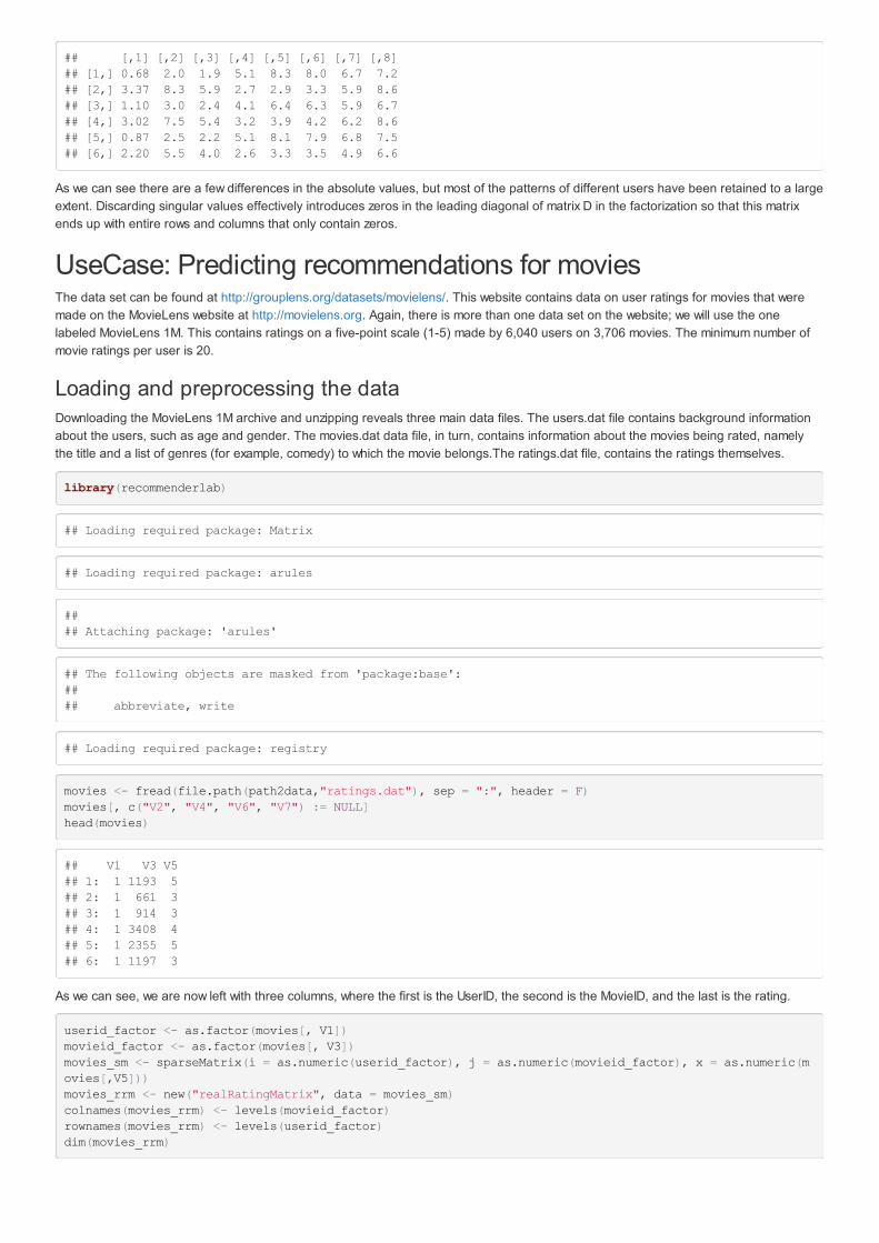
## [,1] [,2] [,3] [,4] [,5] [,6] [,7] [,8]## [1,] 0.68 2.0 1.9 5.1 8.3 8.0 6.7 7.2## [2,] 3.37 8.3 5.9 2.7 2.9 3.3 5.9 8.6## [3,] 1.10 3.0 2.4 4.1 6.4 6.3 5.9 6.7## [4,] 3.02 7.5 5.4 3.2 3.9 4.2 6.2 8.6## [5,] 0.87 2.5 2.2 5.1 8.1 7.9 6.8 7.5## [6,] 2.20 5.5 4.0 2.6 3.3 3.5 4.9 6.6

As we can see there are a few differences in the absolute values, but most of the patterns of different users have been retained to a largeextent. Discarding singular values effectively introduces zeros in the leading diagonal of matrix D in the factorization so that this matrixends up with entire rows and columns that only contain zeros.

UseCase: Predicting recommendations for moviesThe data set can be found at http://grouplens.org/datasets/movielens/. This website contains data on user ratings for movies that weremade on the MovieLens website at http://movielens.org. Again, there is more than one data set on the website; we will use the onelabeled MovieLens 1M. This contains ratings on a five-point scale (1-5) made by 6,040 users on 3,706 movies. The minimum number ofmovie ratings per user is 20.

Loading and preprocessing the dataDownloading the MovieLens 1M archive and unzipping reveals three main data files. The users.dat file contains background informationabout the users, such as age and gender. The movies.dat data file, in turn, contains information about the movies being rated, namelythe title and a list of genres (for example, comedy) to which the movie belongs.The ratings.dat file, contains the ratings themselves.

library(recommenderlab)

## Loading required package: Matrix

## Loading required package: arules

## ## Attaching package: 'arules'

## The following objects are masked from 'package:base':## ## abbreviate, write

## Loading required package: registry

movies <- fread(file.path(path2data,"ratings.dat"), sep = ":", header = F)movies[, c("V2", "V4", "V6", "V7") := NULL]head(movies)

## V1 V3 V5## 1: 1 1193 5## 2: 1 661 3## 3: 1 914 3## 4: 1 3408 4## 5: 1 2355 5## 6: 1 1197 3

As we can see, we are now left with three columns, where the first is the UserID, the second is the MovieID, and the last is the rating.

userid_factor <- as.factor(movies[, V1])movieid_factor <- as.factor(movies[, V3])movies_sm <- sparseMatrix(i = as.numeric(userid_factor), j = as.numeric(movieid_factor), x = as.numeric(movies[,V5]))movies_rrm <- new("realRatingMatrix", data = movies_sm)colnames(movies_rrm) <- levels(movieid_factor)rownames(movies_rrm) <- levels(userid_factor)dim(movies_rrm)

## [1] 6040 3706

Exploring the datawe can make use of the getRatings() function to retrieve the ratings from a rating matrix. This is useful in order to construct a histogram ofitem ratings. Additionally, we can also normalize the ratings with respect to each user. The following code snippet shows how we cancompute ratings and normalized ratings for the MovieLens data and produce histograms for the ratings:

movies_ratings <- getRatings(movies_rrm)movies_normalized_ratings <- getRatings(normalize(movies_rrm, method = "Z-score"))hist(movies_ratings, ylab = "Number of Movies", xlab = "Rating", main = "Histogram of Raw rating")

hist(movies_normalized_ratings, ylab = "Number of Movies",xlab = "Ratings", main = "Histogram of Normalized rating", breaks = 100)

For the MovieLens data with

the 5-point rating scale, 4 is the most prominent rating and higher ratings are far more common than low ratings.

We can also look for the distribution of the number of items rated per user and the average rating per item by looking at the row countsand the column means of the rating matrix respectively.

movies_items_rated_per_user <- rowCounts(movies_rrm)movies_average_item_rating_per_item <- colMeans(movies_rrm)hist(movies_items_rated_per_user, breaks = 100,xlab = "no of movies rated per user", ylab = "Number of Users", main = "Histogram of items rated per user")

hist(movies_average_item_rating_per_item, breaks = 15, main = "Histogram of average rating per item", ylab = "Number of movies" , xlab = "Average rating per movie")

Most of the users have rated very few items, but a small number of very committed users have actually rated a very large number ofitems.

We can find the average of these distributions in order to determine the average number of items rated per user and the average ratingof each item.

(movies_avg_items_rated_per_user <- mean(rowCounts(movies_rrm)))

## [1] 166

(movies_avg_item_rating <- mean(colMeans(movies_rrm)))

## [1] 3.2

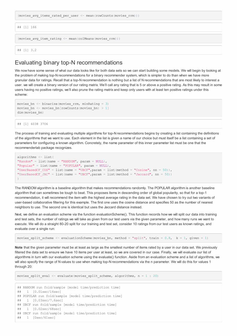
Evaluating binary top-N recommendationsWe now have some sense of what our data looks like for both data sets so we can start building some models. We will begin by looking atthe problem of making top-N recommendations for a binary recommender system, which is simpler to do than when we have moregranular data for ratings. Recall that a top-N recommendation is nothing but a list of N recommendations that are most likely to interest auser. we will create a binary version of our rating matrix. We’ll call any rating that is 5 or above a positive rating. As this may result in someusers having no positive ratings, we’ll also prune the rating matrix and keep only users with at least ten positive ratings under thisscheme:

movies_bn <- binarize(movies_rrm, minRating = 3)movies_bn <- movies_bn[rowCounts(movies_bn) > 1]dim(movies_bn)

## [1] 6038 3706

The process of training and evaluating multiple algorithms for top-N recommendations begins by creating a list containing the definitionsof the algorithms that we want to use. Each element in the list is given a name of our choice but must itself be a list containing a set ofparameters for configuring a known algorithm. Concretely, the name parameter of this inner parameter list must be one that therecommenderlab package recognizes.

algorithms <- list("Random" = list(name = "RANDOM", param = NULL),"Popular" = list(name = "POPULAR", param = NULL),"UserBasedCF_COS" = list(name = "UBCF",param = list(method = "Cosine", nn = 50)),"UserBasedCF_JAC" = list(name = "UBCF",param = list(method = "Jaccard", nn = 50)))

The RANDOM algorithm is a baseline algorithm that makes recommendations randomly. The POPULAR algorithm is another baselinealgorithm that can sometimes be tough to beat. This proposes items in descending order of global popularity, so that for a top-1recommendation, it will recommend the item with the highest average rating in the data set. We have chosen to try out two variants ofuser-based collaborative filtering for this example. The first one uses the cosine distance and specifies 50 as the number of nearestneighbors to use. The second one is identical but uses the Jaccard distance instead.

Next, we define an evaluation scheme via the function evaluationScheme(). This function records how we will split our data into trainingand test sets, the number of ratings we will take as given from our test users via the given parameter, and how many runs we want toexecute. We will do a straight 80-20 split for our training and test set, consider 10 ratings from our test users as known ratings, andevaluate over a single run:

movies_split_scheme <- evaluationScheme(movies_bn, method = "split", train = 0.8, k = 1, given = 1)

Note that the given parameter must be at least as large as the smallest number of items rated by a user in our data set. We previouslyfiltered the data set to ensure we have 10 items per user at least, so we are covered in our case. Finally, we will evaluate our list ofalgorithms in turn with our evaluation scheme using the evaluate() function. Aside from an evaluation scheme and a list of algorithms, wewill also specify the range of N values to use when making top-N recommendations via the n parameter. We will do this for values 1through 20:

movies_split_eval <- evaluate(movies_split_scheme, algorithms, n = 1 : 20)

## RANDOM run fold/sample [model time/prediction time]## 1 [0.01sec/14sec] ## POPULAR run fold/sample [model time/prediction time]## 1 [0.03sec/7.6sec] ## UBCF run fold/sample [model time/prediction time]## 1 [0.02sec/68sec] ## UBCF run fold/sample [model time/prediction time]## 1 [0sec/61sec]

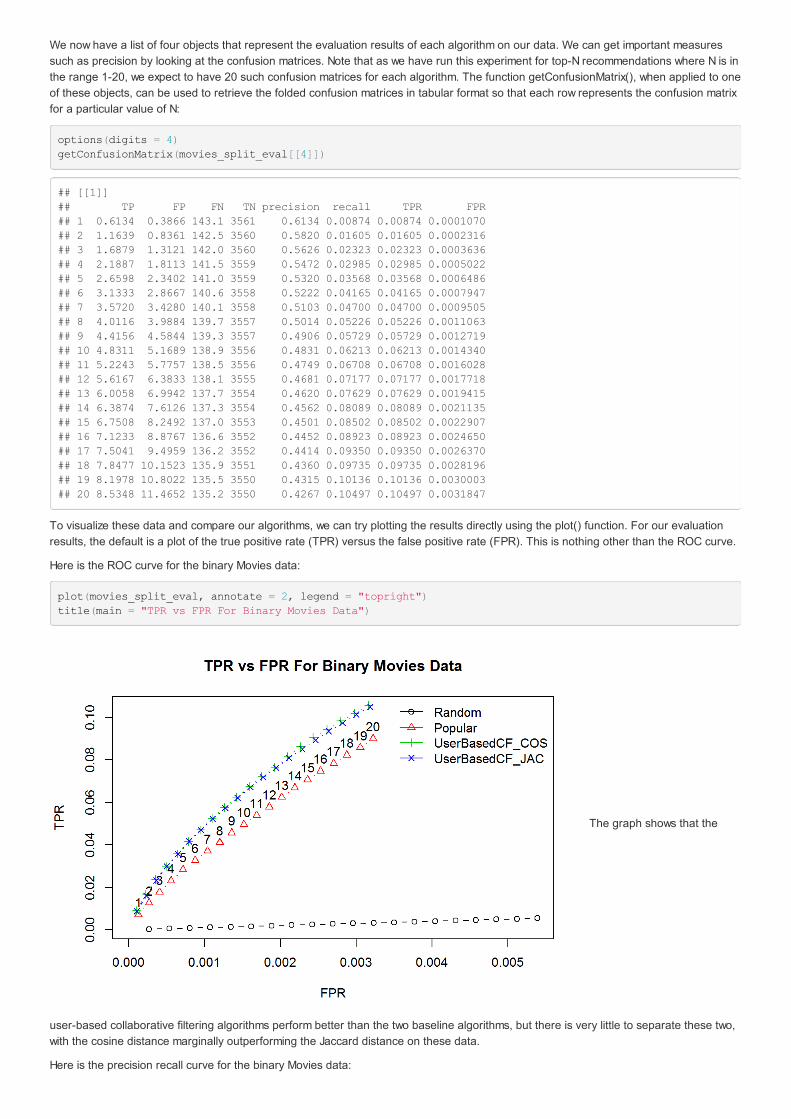
We now have a list of four objects that represent the evaluation results of each algorithm on our data. We can get important measuressuch as precision by looking at the confusion matrices. Note that as we have run this experiment for top-N recommendations where N is inthe range 1-20, we expect to have 20 such confusion matrices for each algorithm. The function getConfusionMatrix(), when applied to oneof these objects, can be used to retrieve the folded confusion matrices in tabular format so that each row represents the confusion matrixfor a particular value of N:

options(digits = 4)getConfusionMatrix(movies_split_eval[[4]])

## [[1]]## TP FP FN TN precision recall TPR FPR## 1 0.6134 0.3866 143.1 3561 0.6134 0.00874 0.00874 0.0001070## 2 1.1639 0.8361 142.5 3560 0.5820 0.01605 0.01605 0.0002316## 3 1.6879 1.3121 142.0 3560 0.5626 0.02323 0.02323 0.0003636## 4 2.1887 1.8113 141.5 3559 0.5472 0.02985 0.02985 0.0005022## 5 2.6598 2.3402 141.0 3559 0.5320 0.03568 0.03568 0.0006486## 6 3.1333 2.8667 140.6 3558 0.5222 0.04165 0.04165 0.0007947## 7 3.5720 3.4280 140.1 3558 0.5103 0.04700 0.04700 0.0009505## 8 4.0116 3.9884 139.7 3557 0.5014 0.05226 0.05226 0.0011063## 9 4.4156 4.5844 139.3 3557 0.4906 0.05729 0.05729 0.0012719## 10 4.8311 5.1689 138.9 3556 0.4831 0.06213 0.06213 0.0014340## 11 5.2243 5.7757 138.5 3556 0.4749 0.06708 0.06708 0.0016028## 12 5.6167 6.3833 138.1 3555 0.4681 0.07177 0.07177 0.0017718## 13 6.0058 6.9942 137.7 3554 0.4620 0.07629 0.07629 0.0019415## 14 6.3874 7.6126 137.3 3554 0.4562 0.08089 0.08089 0.0021135## 15 6.7508 8.2492 137.0 3553 0.4501 0.08502 0.08502 0.0022907## 16 7.1233 8.8767 136.6 3552 0.4452 0.08923 0.08923 0.0024650## 17 7.5041 9.4959 136.2 3552 0.4414 0.09350 0.09350 0.0026370## 18 7.8477 10.1523 135.9 3551 0.4360 0.09735 0.09735 0.0028196## 19 8.1978 10.8022 135.5 3550 0.4315 0.10136 0.10136 0.0030003## 20 8.5348 11.4652 135.2 3550 0.4267 0.10497 0.10497 0.0031847

To visualize these data and compare our algorithms, we can try plotting the results directly using the plot() function. For our evaluationresults, the default is a plot of the true positive rate (TPR) versus the false positive rate (FPR). This is nothing other than the ROC curve.

Here is the ROC curve for the binary Movies data:

plot(movies_split_eval, annotate = 2, legend = "topright")title(main = "TPR vs FPR For Binary Movies Data")

The graph shows that the

user-based collaborative filtering algorithms perform better than the two baseline algorithms, but there is very little to separate these two,with the cosine distance marginally outperforming the Jaccard distance on these data.

Here is the precision recall curve for the binary Movies data:

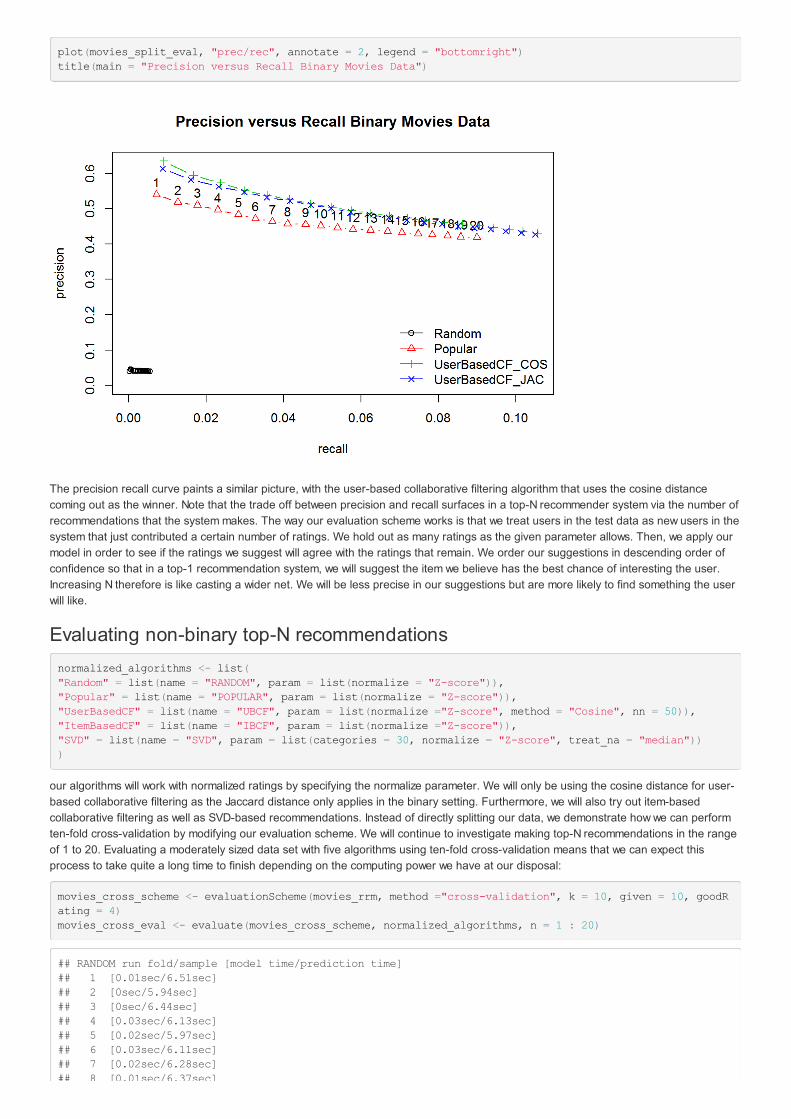
plot(movies_split_eval, "prec/rec", annotate = 2, legend = "bottomright")title(main = "Precision versus Recall Binary Movies Data")

The precision recall curve paints a similar picture, with the user-based collaborative filtering algorithm that uses the cosine distancecoming out as the winner. Note that the trade off between precision and recall surfaces in a top-N recommender system via the number ofrecommendations that the system makes. The way our evaluation scheme works is that we treat users in the test data as new users in thesystem that just contributed a certain number of ratings. We hold out as many ratings as the given parameter allows. Then, we apply ourmodel in order to see if the ratings we suggest will agree with the ratings that remain. We order our suggestions in descending order ofconfidence so that in a top-1 recommendation system, we will suggest the item we believe has the best chance of interesting the user.Increasing N therefore is like casting a wider net. We will be less precise in our suggestions but are more likely to find something the userwill like.

Evaluating non-binary top-N recommendationsnormalized_algorithms <- list("Random" = list(name = "RANDOM", param = list(normalize = "Z-score")),"Popular" = list(name = "POPULAR", param = list(normalize = "Z-score")),"UserBasedCF" = list(name = "UBCF", param = list(normalize ="Z-score", method = "Cosine", nn = 50)),"ItemBasedCF" = list(name = "IBCF", param = list(normalize ="Z-score")),"SVD" = list(name = "SVD", param = list(categories = 30, normalize = "Z-score", treat_na = "median")))

our algorithms will work with normalized ratings by specifying the normalize parameter. We will only be using the cosine distance for user-based collaborative filtering as the Jaccard distance only applies in the binary setting. Furthermore, we will also try out item-basedcollaborative filtering as well as SVD-based recommendations. Instead of directly splitting our data, we demonstrate how we can performten-fold cross-validation by modifying our evaluation scheme. We will continue to investigate making top-N recommendations in the rangeof 1 to 20. Evaluating a moderately sized data set with five algorithms using ten-fold cross-validation means that we can expect thisprocess to take quite a long time to finish depending on the computing power we have at our disposal:

movies_cross_scheme <- evaluationScheme(movies_rrm, method ="cross-validation", k = 10, given = 10, goodRating = 4)movies_cross_eval <- evaluate(movies_cross_scheme, normalized_algorithms, n = 1 : 20)

## RANDOM run fold/sample [model time/prediction time]## 1 [0.01sec/6.51sec] ## 2 [0sec/5.94sec] ## 3 [0sec/6.44sec] ## 4 [0.03sec/6.13sec] ## 5 [0.02sec/5.97sec] ## 6 [0.03sec/6.11sec] ## 7 [0.02sec/6.28sec] ## 8 [0.01sec/6.37sec]

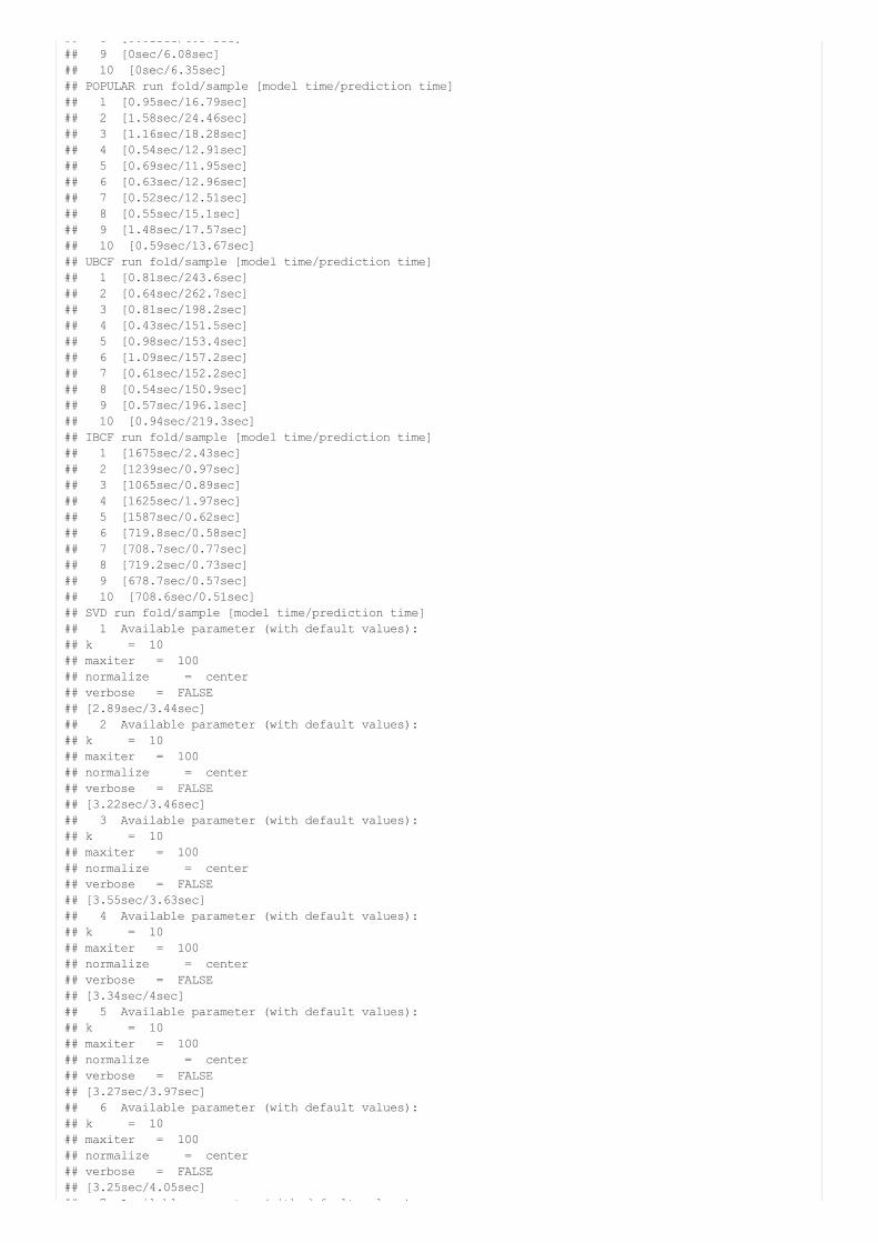
## 8 [0.01sec/6.37sec] ## 9 [0sec/6.08sec] ## 10 [0sec/6.35sec] ## POPULAR run fold/sample [model time/prediction time]## 1 [0.95sec/16.79sec] ## 2 [1.58sec/24.46sec] ## 3 [1.16sec/18.28sec] ## 4 [0.54sec/12.91sec] ## 5 [0.69sec/11.95sec] ## 6 [0.63sec/12.96sec] ## 7 [0.52sec/12.51sec] ## 8 [0.55sec/15.1sec] ## 9 [1.48sec/17.57sec] ## 10 [0.59sec/13.67sec] ## UBCF run fold/sample [model time/prediction time]## 1 [0.81sec/243.6sec] ## 2 [0.64sec/262.7sec] ## 3 [0.81sec/198.2sec] ## 4 [0.43sec/151.5sec] ## 5 [0.98sec/153.4sec] ## 6 [1.09sec/157.2sec] ## 7 [0.61sec/152.2sec] ## 8 [0.54sec/150.9sec] ## 9 [0.57sec/196.1sec] ## 10 [0.94sec/219.3sec] ## IBCF run fold/sample [model time/prediction time]## 1 [1675sec/2.43sec] ## 2 [1239sec/0.97sec] ## 3 [1065sec/0.89sec] ## 4 [1625sec/1.97sec] ## 5 [1587sec/0.62sec] ## 6 [719.8sec/0.58sec] ## 7 [708.7sec/0.77sec] ## 8 [719.2sec/0.73sec] ## 9 [678.7sec/0.57sec] ## 10 [708.6sec/0.51sec] ## SVD run fold/sample [model time/prediction time]## 1 Available parameter (with default values):## k = 10## maxiter = 100## normalize = center## verbose = FALSE## [2.89sec/3.44sec] ## 2 Available parameter (with default values):## k = 10## maxiter = 100## normalize = center## verbose = FALSE## [3.22sec/3.46sec] ## 3 Available parameter (with default values):## k = 10## maxiter = 100## normalize = center## verbose = FALSE## [3.55sec/3.63sec] ## 4 Available parameter (with default values):## k = 10## maxiter = 100## normalize = center## verbose = FALSE## [3.34sec/4sec] ## 5 Available parameter (with default values):## k = 10## maxiter = 100## normalize = center## verbose = FALSE## [3.27sec/3.97sec] ## 6 Available parameter (with default values):## k = 10## maxiter = 100## normalize = center## verbose = FALSE## [3.25sec/4.05sec] ## 7 Available parameter (with default values):

## 7 Available parameter (with default values):## k = 10## maxiter = 100## normalize = center## verbose = FALSE## [3.17sec/4.12sec] ## 8 Available parameter (with default values):## k = 10## maxiter = 100## normalize = center## verbose = FALSE## [3.25sec/4.03sec] ## 9 Available parameter (with default values):## k = 10## maxiter = 100## normalize = center## verbose = FALSE## [3.52sec/3.7sec] ## 10 Available parameter (with default values):## k = 10## maxiter = 100## normalize = center## verbose = FALSE## [3.39sec/3.88sec]

Here is the ROC curve for the MovieLens data:

plot(movies_cross_eval, annotate = 4, legend = "topright")title(main = "TPR versus FPR For Movielens Data")

As we can see, user-based

collaborative filtering is the clear winner here. SVD performs in a similar manner to the POPULAR baseline, though the latter starts tobecome better when N is high. Finally, we see item-based collaborative filtering performing far worse than these, outperforming only therandom baseline. What is clear from these experiments is that tuning recommendation systems can often be a very time-consuming,resource-intensive endeavor.

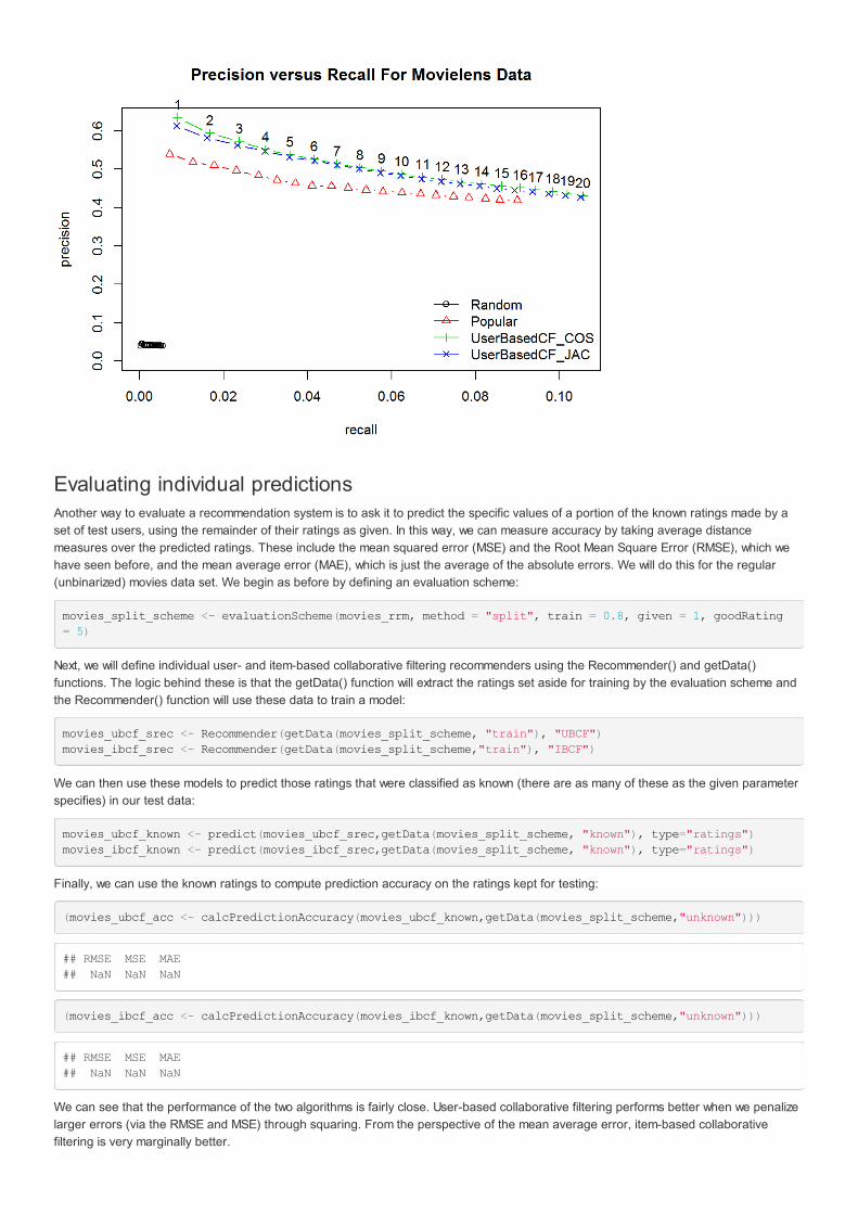
we will plot the precision recall curve for the MovieLens data. Here is the precision recall curve for the MovieLens data:

plot(movies_split_eval, "prec/rec", annotate = 3,legend = "bottomright")title(main = "Precision versus Recall For Movielens Data")

Evaluating individual predictionsAnother way to evaluate a recommendation system is to ask it to predict the specific values of a portion of the known ratings made by aset of test users, using the remainder of their ratings as given. In this way, we can measure accuracy by taking average distancemeasures over the predicted ratings. These include the mean squared error (MSE) and the Root Mean Square Error (RMSE), which wehave seen before, and the mean average error (MAE), which is just the average of the absolute errors. We will do this for the regular(unbinarized) movies data set. We begin as before by defining an evaluation scheme:

movies_split_scheme <- evaluationScheme(movies_rrm, method = "split", train = 0.8, given = 1, goodRating = 5)

Next, we will define individual user- and item-based collaborative filtering recommenders using the Recommender() and getData()functions. The logic behind these is that the getData() function will extract the ratings set aside for training by the evaluation scheme andthe Recommender() function will use these data to train a model:

movies_ubcf_srec <- Recommender(getData(movies_split_scheme, "train"), "UBCF")movies_ibcf_srec <- Recommender(getData(movies_split_scheme,"train"), "IBCF")

We can then use these models to predict those ratings that were classified as known (there are as many of these as the given parameterspecifies) in our test data:

movies_ubcf_known <- predict(movies_ubcf_srec,getData(movies_split_scheme, "known"), type="ratings")movies_ibcf_known <- predict(movies_ibcf_srec,getData(movies_split_scheme, "known"), type="ratings")

Finally, we can use the known ratings to compute prediction accuracy on the ratings kept for testing:

(movies_ubcf_acc <- calcPredictionAccuracy(movies_ubcf_known,getData(movies_split_scheme,"unknown")))

## RMSE MSE MAE ## NaN NaN NaN

(movies_ibcf_acc <- calcPredictionAccuracy(movies_ibcf_known,getData(movies_split_scheme,"unknown")))

## RMSE MSE MAE ## NaN NaN NaN

We can see that the performance of the two algorithms is fairly close. User-based collaborative filtering performs better when we penalizelarger errors (via the RMSE and MSE) through squaring. From the perspective of the mean average error, item-based collaborativefiltering is very marginally better.

Consequently, in this case, we might make our decision on which type of recommendation system to use on the basis of the errorbehavior that more closely matches our business needs. In this section, we used the default parameter values for the two algorithms, butby using the parameter parameter in the Recommender() function, we can play around with different configurations as we did before. Thisis left as an exercise for the reader.

Referrences :https://en.wikipedia.org/wiki/Collaborative_filteringhttp://infolab.stanford.edu/~ullman/mmds/ch9.pdfhttp://www.sciencedirect.com/science/article/pii/S1110866515000341Mastering Predictive Analytics with R : Rui Miguel Forte