New data structures and algorithms forpost-processing large data sets and multi-variate

functions in spatio-temporal statistics

Alexander Litvinenko∗,joint work with D. Keyes, V. Khoromskaia,

B.Khoromskij and H.G. Matthies

∗Bayesian Computing group, Extreme Computing Research Center and SRI UQ

http://sri-uq.kaust.edu.sa/

4*

Outline

Motivation and Introduction

Examples with tensors of order 2

Higher order tensors

Five tasks in statistics to solve

Tensor approximation of Matern covariance, trace, diagonal, anddeterminant

2 / 36

4*

Motivation: Low-rank data approximation

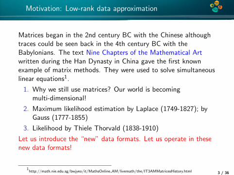
Matrices began in the 2nd century BC with the Chinese althoughtraces could be seen back in the 4th century BC with theBabylonians. The text Nine Chapters of the Mathematical Artwritten during the Han Dynasty in China gave the first knownexample of matrix methods. They were used to solve simultaneouslinear equations1.

1. Why we still use matrices? Our world is becomingmulti-dimensional!

2. Maximum likelihood estimation by Laplace (1749-1827); byGauss (1777-1855)

3. Likelihood by Thiele Thorvald (1838-1910)

Let us introduce the “new” data formats. Let us operate in thesenew data formats!

1http://math.nie.edu.sg/bwjyeo/it/MathsOnline AM/livemath/the/IT3AMMatricesHistory.html 3 / 36

4*

Tensor

I

I

I2

3

1

I3A

I2

A(1)I1

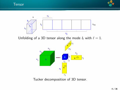
Unfolding of a 3D tensor along the mode I` with ` = 1.r3

3

2

r

1

r

r

r1

B

1

32

r2

A

V

(1)

V(2)

V

(3)

n

n

n

n1

n3

n2

Tucker decomposition of 3D tensor.

4 / 36

4*

Curse of dimensionality

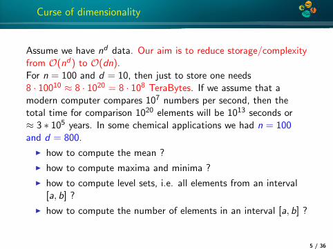
Assume we have nd data. Our aim is to reduce storage/complexityfrom O(nd) to O(dn).For n = 100 and d = 10, then just to store one needs8 · 10010 ≈ 8 · 1020 = 8 · 108 TeraBytes. If we assume that amodern computer compares 107 numbers per second, then thetotal time for comparison 1020 elements will be 1013 seconds or≈ 3 ∗ 105 years. In some chemical applications we had n = 100and d = 800.

I how to compute the mean ?

I how to compute maxima and minima ?

I how to compute level sets, i.e. all elements from an interval[a, b] ?

I how to compute the number of elements in an interval [a, b] ?

5 / 36

4*

Why tensors are working?

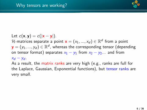
Let c(x, y) = c(|x− y|).H-matrices separate a point x = (x1, ..., xd) ∈ Rd from a pointy = (y1, ..., yd) ∈ Rd , whereas the corresponding tensor (dependingon tensor format) separates x1 − y1 from x2 − y2... and fromxd − yd .As a result, the matrix ranks are very high (e.g., ranks are full forthe Laplace, Gaussian, Exponential functions), but tensor ranks arevery small.

6 / 36

4*

Properties of low-rank matrices: Arithmetic operations

Let v ∈ Rm be a measurement or a snapshot. LetM := [v1, v2, ..., vm] be a matrix of m snapshots.Suppose M ≈ Mk = ABT ∈ Rn×m, A ∈ Rn×k , B ∈ Rm×k is given.

Property 1: Mkv = ABTv = (A(BTv)). Cost O(km + kn).

Suppose M′

= CDT , C ∈ Rn×k and D ∈ Rm×k .

Property 2: Mk + M′

= AnewBTnew, Anew := [AC ] ∈ Rn×2k and

Bnew = [B D] ∈ Rm×2k .

Cost of rank truncation from 2k to k is O((n + m)k2 + k3).

7 / 36

4*

Example from CFD and aerodynamics

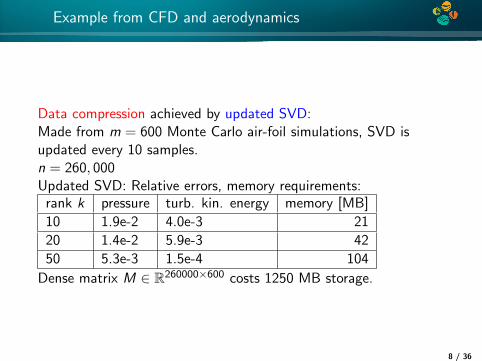
Data compression achieved by updated SVD:Made from m = 600 Monte Carlo air-foil simulations, SVD isupdated every 10 samples.n = 260, 000Updated SVD: Relative errors, memory requirements:

rank k pressure turb. kin. energy memory [MB]

10 1.9e-2 4.0e-3 21

20 1.4e-2 5.9e-3 42

50 5.3e-3 1.5e-4 104

Dense matrix M ∈ R260000×600 costs 1250 MB storage.

8 / 36

4*

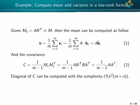
Example: Compute mean and variance in a low-rank format

Given Mk = ABT ≈ M, then the mean can be computed as follow

v =1

m

m∑i=1

vi =1

m

m∑i=1

A · bi = Ab, (1)

And the covariance

C =1

m − 1McM

Tc =

1

m − 1ABTBAT =

1

m − 1AAT . (2)

Diagonal of C can be computed with the complexity O(k2(m+n)).

9 / 36

Higher order tensors

10 / 36

4*

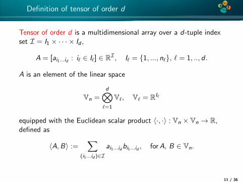
Definition of tensor of order d

Tensor of order d is a multidimensional array over a d-tuple indexset I = I1 × · · · × Id ,

A = [ai1...id : i` ∈ I`] ∈ RI , I` = {1, ..., n`}, ` = 1, .., d .

A is an element of the linear space

Vn =d⊗`=1

V`, V` = RI`

equipped with the Euclidean scalar product 〈·, ·〉 : Vn × Vn → R,defined as

〈A,B〉 :=∑

(i1...id )∈I

ai1...idbi1...id , forA, B ∈ Vn.

11 / 36

4*

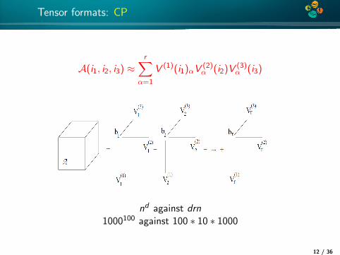
Tensor formats: CP

A(i1, i2, i3) ≈r∑

α=1

V (1)(i1)αV(2)α (i2)V (3)

α (i3)

nd against drn1000100 against 100 ∗ 10 ∗ 1000

12 / 36

4*

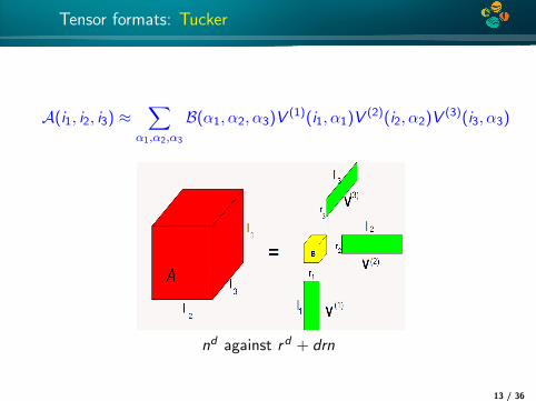
Tensor formats: Tucker

A(i1, i2, i3) ≈∑

α1,α2,α3

B(α1, α2, α3)V (1)(i1, α1)V (2)(i2, α2)V (3)(i3, α3)

nd against rd + drn

13 / 36

4*

Tensor formats: tensor train TT

[Tyrtyshnikov, Oseledets, et al 2010-now]

A(i1, ..., id) ≈∑

α1,...,αd−1

G1(i1, α1)G2(α1, i2, α2)...Gd−1(αd−1, id)

[http://stockfresh.com/image/293793/children-on-train]Computation of a single element in the canonical format takes O(dr) operations, so the expected cost of the

TT-cross approximation method in this situation is O(d2nr2 + dnr3).

14 / 36

4*

Tensor and Matrices

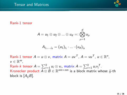
Rank-1 tensor

A = u1 ⊗ u2 ⊗ ...⊗ ud =:d⊗µ=1

uµ

Ai1,...,id = (u1)i1 · ... · (ud)id

Rank-1 tensor A = u ⊗ v , matrix A = uvT , A = vuT , u ∈ Rn,v ∈ Rm,Rank-k tensor A =

∑ki=1 ui ⊗ vi , matrix A =

∑ki=1 uiv

Ti .

Kronecker product A⊗ B ∈ Rnm×nm is a block matrix whose ij-thblock is [AijB].

15 / 36

4*

Five tasks in statistics to solve

Task 1. Approximate a Matern covariance function in a low-ranktensor format.‖c(x, y)−

∑ri=1

∏dµ=1 ciµ(xµ, yµ)‖ ≤ ε, for some given ε > 0.

Alternatively, we may look for factors Ciµ such that

‖C−∑r

i=1

⊗dµ=1 Ciµ‖ ≤ ε. Here, matrices Ciµ correspond to the

one-dimensional functions ciµ(xµ, yµ) in the direction µ.

Task 2. Computing of square root of C. The square root C1/2 ofthe covariance matrix C is needed in order to generate randomfields and processes. It is also used in the Kalman filter update.

Task 3. Kriging.The kriging estimate s is given by s = CsyC−1yy y.

16 / 36

4*

Five tasks in statistics to solve

Task 4. Geostatistical design.

ϕA = N−1 trace[Css|y

], and ϕC = zT (Css|y )z, (3)

where Css|y := Css − CsyC−1yy Cys

Task 5. Computing the joint Gaussian log-likelihood function.

L(θ) = −N

2log(2π)− 1

2log det{C(θ)} − 1

2(zT · C(θ)−1z). (4)

17 / 36

4*

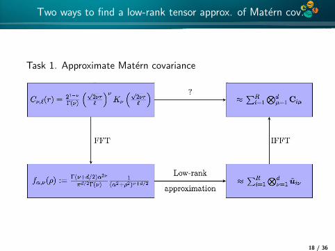
Two ways to find a low-rank tensor approx. of Matern cov.

Task 1. Approximate Matern covariance

18 / 36

4*

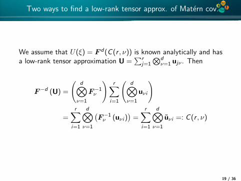
Two ways to find a low-rank tensor approx. of Matern cov.

We assume that U(ξ) = F d(C (r , ν)) is known analytically and hasa low-rank tensor approximation U =

∑rj=1

⊗dν=1 ujν . Then

F−d (U) =

(d⊗ν=1

F−1ν

)r∑

i=1

(d⊗ν=1

uνi

)

=r∑

i=1

d⊗ν=1

(F−1ν (uνi )

)=

r∑i=1

d⊗ν=1

uνi =: C (r , ν)

19 / 36

4*

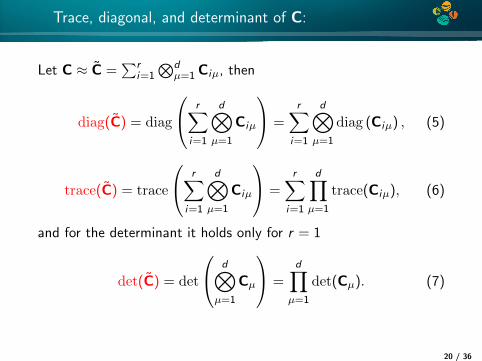
Trace, diagonal, and determinant of C:

Let C ≈ C =∑r

i=1

⊗dµ=1 Ciµ, then

diag(C) = diag

r∑i=1

d⊗µ=1

Ciµ

=r∑

i=1

d⊗µ=1

diag (Ciµ) , (5)

trace(C) = trace

r∑i=1

d⊗µ=1

Ciµ

=r∑

i=1

d∏µ=1

trace(Ciµ), (6)

and for the determinant it holds only for r = 1

det(C) = det

d⊗µ=1

Cµ

=d∏µ=1

det(Cµ). (7)

20 / 36

4*

Existence of the canonical low-rank tensor approximation

A scheme of the proof of existence of the canonical low-rank tensorapproximation. See details in [A. Litvinenko, et al., Tucker Tensor analysis of Matern

functions in spatial statistics, preprint arXiv:1711.06874, 2017]

It could be easier to apply the Laplace transform to the Fouriertransform of a Matern covariance matrix, than to the Materncovariance. To approximate the resulting Laplace integral we applythe sinc quadrature.

21 / 36

4*

Numerics: relative error vs Tucker rank

C (x, y) = e−‖x−y‖, x, y ∈ R3

5 10 15

Tucker rank

10-10

10-5

err

or

N=653

N=1293

N=2573

N=5133

Relative error‖Q−Q(r)‖‖Q‖ , where Q(r) is the tensor reconstructed

from the Tucker rank-r decomposition of Q vs Tucker ranks.

Tucker rank r 1 4 10

n=129 0.386 0.017 7.5e-6

n=257 0.386 0.073 1.4e-5

n=513 0.386 0.073 0.003522 / 36

4*

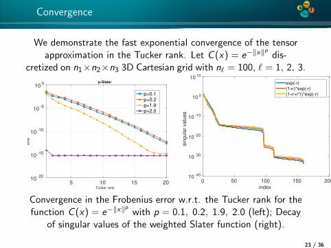
Convergence

We demonstrate the fast exponential convergence of the tensorapproximation in the Tucker rank. Let C (x) = e−‖x‖

pdis-

cretized on n1×n2×n3 3D Cartesian grid with n` = 100, ` = 1, 2, 3.

Tucker rank

5 10 15 20

err

or

10-20

10-15

10-10

10-5

100 p-Slater

p=0.1p=0.2p=1.9p=2.0

index

0 50 100 150 200sin

gula

r valu

es

10 -40

10 -30

10 -20

10 -10

10 0

10 10

exp(-r)

(1+r)*exp(-r)

(1+r+r*r)*exp(-r)

Convergence in the Frobenius error w.r.t. the Tucker rank for thefunction C (x) = e−‖x‖

pwith p = 0.1, 0.2, 1.9, 2.0 (left); Decay

of singular values of the weighted Slater function (right).

23 / 36

4*

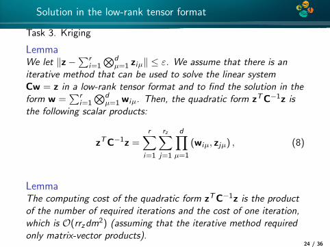
Solution in the low-rank tensor format

Task 3. Kriging

LemmaWe let ‖z−

∑ri=1

⊗dµ=1 ziµ‖ ≤ ε. We assume that there is an

iterative method that can be used to solve the linear systemCw = z in a low-rank tensor format and to find the solution in theform w =

∑ri=1

⊗dµ=1wiµ. Then, the quadratic form zTC−1z is

the following scalar products:

zTC−1z =r∑

i=1

rz∑j=1

d∏µ=1

(wiµ, zjµ) , (8)

LemmaThe computing cost of the quadratic form zTC−1z is the productof the number of required iterations and the cost of one iteration,which is O(rrzdm

2) (assuming that the iterative method requiredonly matrix-vector products).

24 / 36

4*

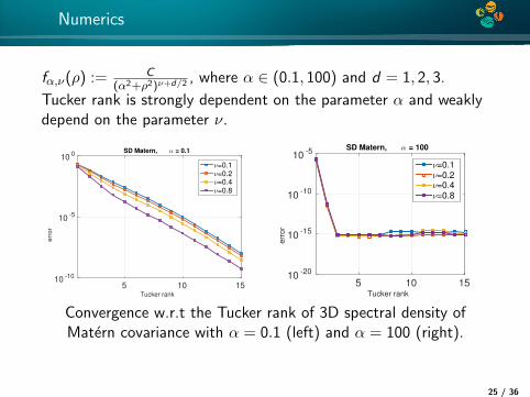
Numerics

fα,ν(ρ) := C(α2+ρ2)ν+d/2 , where α ∈ (0.1, 100) and d = 1, 2, 3.

Tucker rank is strongly dependent on the parameter α and weaklydepend on the parameter ν.

Tucker rank

5 10 15

err

or

10-10

10-5

100

SD Matern, α = 0.1

ν=0.1

ν=0.2

ν=0.4

ν=0.8

Tucker rank

5 10 15e

rro

r10

-20

10-15

10-10

10-5

SD Matern, α = 100

ν=0.1

ν=0.2

ν=0.4

ν=0.8

Convergence w.r.t the Tucker rank of 3D spectral density ofMatern covariance with α = 0.1 (left) and α = 100 (right).

25 / 36

4*

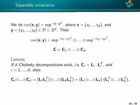
Separable covariance

We let cov(x, y) = exp−|x−y|2, where x = (x1, .., xd), and

y = (y1, ..., yd) ∈ D ⊂ Rd . Then

cov(x, y) = exp−|x1−y1|2 ⊗ . . .⊗ exp−|xd−yd |

2.

C = C1 ⊗ ...⊗ Cd .

LemmaIf d Cholesky decompositions exist, i.e, Ci = Li · LTi , andi = 1, ..., d , then

C1⊗...⊗Cd = (L1LT1 )⊗...⊗(LdL

Td ) = (L1⊗...⊗Ld)·(LT1 ⊗...⊗LTd ),

26 / 36

4*

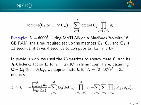
log det()

log det(C1 ⊗ . . .⊗ Cd) =d∑

j=1

log detCj

d∏i=1,i 6=j

ni .

Example: N = 60003. Using MATLAB on a MacBookPro with 16GB RAM, the time required set up the matrices C1, C2, and C3 is11 seconds; it takes 4 seconds to compute L1, L2, and L3.

In previous work we used the H-matrices to approximate Ci and itsH-Cholesky factor Li for n = 2 · 106 in 2 minutes. Here, assumingC = C1 ⊗ . . .⊗ Cd , we approximate C for N = (2 · 106)d in 2dminutes.

L ≈ L = −∏dν=1 nν

log(2π)−

d∑j=1

log detCj

d∏i=1,i 6=j

ni−r∑

i=1

r∑j=1

d∏ν=1

(uTi ,ν ,uj ,ν).

27 / 36

4*

Conclusion

Today we discussed:

I Motivation: why do we need low-rank tensors

I Tensors of the second and higher orders

I CP, Tucker and tensor train tensor formats

I Fourier transform of Matern function is easier to approximateas Matern itself

I Proof that Matern covariance has a low-rank CPrepresentation (via Laplace transform and sinc-quadrature)

I Dependence of tensor ranks on parameters of Materncovariance

I Five typical statistical tasks in CP low-rank tensor format.

28 / 36

4*

Tensor Software, you can Click!Click!Click!

Ivan Oseledets et al., Tensor Train toolbox (Matlab)

D.Kressner, C. Tobler, Hierarchical Tucker Toolbox (Matlab)

M. Espig, et al, Tensor Calculus library (in C)

Vervliet N., Debals O., Sorber L., Van Barel M. and De LathauwerL., TensorLab

29 / 36

4*

Literature

1. A. Litvinenko, D. Keyes, V. Khoromskaia, B.N. Khoromskij, H.G.Matthies, Tucker Tensor analysis of Matern functions in spatial statistics,preprint arXiv:1711.06874, 2017

2. A. Litvinenko, HLIBCov: Parallel Hierarchical Matrix Approximation ofLarge Covariance Matrices and Likelihoods with Applications inParameter Identification, preprint arXiv:1709.08625, 2017

3. A. Litvinenko, Y. Sun, M.G. Genton, D. Keyes, Likelihood ApproximationWith Hierarchical Matrices For Large Spatial Datasets, preprintarXiv:1709.04419, 2017

4. B.N. Khoromskij, A. Litvinenko, H.G. Matthies, Application ofhierarchical matrices for computing the Karhunen-Loeve expansion,Computing 84 (1-2), 49-67, 2009

30 / 36

4*

Literature

6. H.G. Matthies, E. Zander, B.V. Rosic, A. Litvinenko, Parameterestimation via conditional expectation: a Bayesian inversion, AdvancedModeling and Simulation in Engineering Sciences 3 (1), 24, 2016

7. H.G. Matthies, A Litvinenko, BV Rosic, E Zander, Bayesian ParameterEstimation via Filtering and Functional Approximations, preprintarXiv:1611.09293, 2016

8. H. G. Matthies, E. Zander, O. Pajonk, B. V. Rosic, A. Litvinenko, InverseProblems in a Bayesian Setting, Computational Methods for Solids andFluids Multiscale Analysis, Probability Aspects and Model ReductionEditors: Ibrahimbegovic, Adnan (Ed.), ISSN: 1871-3033, pp 245-286,2016

9. A. Litvinenko, Application of hierarchical matrices for solving multiscaleproblems, Dissertation, Leipzig University, Germany,http://www.wire.tu-bs.de/mitarbeiter/litvinen/diss.pdf, 2006

10. W. Nowak, A. Litvinenko, Kriging and spatial design accelerated byorders of magnitude: Combining low-rank covariance approximations withFFT-techniques, Mathematical Geosciences 45 (4), 411-435, 2013

31 / 36

4*

Used Literature and Slides

I Book of W. Hackbusch 2012,

I Dissertations of I. Oseledets and M. Espig

I Articles of Tyrtyshnikov et al., De Lathauwer et al., L.Grasedyck, B. Khoromskij, M. Espig

I Lecture courses and presentations of Boris and VeneraKhoromskij

I Software T. Kolda et al.; M. Espig et al.; D. Kressner, K.Tobler; I. Oseledets et al.

32 / 36

4*

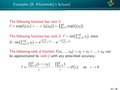
Examples (B. Khoromskij’s lecture)

The following function has rank 1:f = exp(f1(x1) + ...+ fd(xd)) =

∏dj=1 exp(fj(xj))

The following function has rank 2: f = sin(∑d

j=1 xj), since

2i · sin(∑d

j=1 xj) = e i∑d

j=1 xj − e−i∑d

j=1 xj

The following rank d function f (x1, ..., xd) = x1 + x2 + ...+ xd canbe approximated by rank-2 with any prescribed accuracy:

f ≈∏d

j=1(1 + εxj)

ε−∏d

j=1 1

ε+O(ε), as ε→ 0

33 / 36

4*

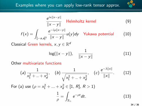
Examples where you can apply low-rank tensor approx.

e iκ‖x−y‖

‖x − y‖Helmholtz kernel (9)

f (x) =

∫[−a,a]3

e−iµ‖x−y‖

‖x − y‖u(y)dy Yukawa potential (10)

Classical Green kernels, x , y ∈ Rd

log(‖x − y‖), 1

‖x − y‖(11)

Other multivariate functions

(a)1

x21 + ..+ x2d, (b)

1√x21 + ..+ x2d

, (c)e−λ‖x‖

‖x‖. (12)

For (a) use (ρ = x21 + ...+ x2d ∈ [1, R], R > 1)

1

ρ=

∫R+

e−ρtdt. (13)

34 / 36

4*

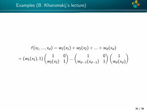
Examples (B. Khoromskij’s lecture)

f (x1, ..., xd) = w1(x1) + w2(x2) + ...+ wd(xd)

= (w1(x1), 1)

(1 0

w2(x2) 1

)...

(1 0

wd−1(xd−1) 1

)(1

wd(xd)

)

35 / 36

4*

Examples:

rank(f )=2

f = sin(x1 + x2 + ...+ xd)

= (sinx1, cosx1)

(cosx2 −sinx2sinx2 cosx2

)...

(cosxd−1 −sinxd−1

sinxd−1 cosxd−1

)(cosxd

sinxd−1

)

36 / 36