Embed Size (px)
Citation preview

.
Multi-Dimensional Modeling with BI A background to the techniques used to create BI InfoCubes Version 1.0 May 16, 2006
Multi-Dimensional Modeling with BI
©2000 SAP AG and SAP America, Inc. Table of Contents
Table of Contents
Table of Contents.................................................................................................................2
1 Introduction.......................................................................................................................3
2 Theoretical Background: From Multi-Dimensional Model to InfoCube......................5
2.1 The goals of multi-dimensional data models ........................................................................................ 5
2.2 Basic Modeling Steps ............................................................................................................................. 5
2.3 Star Schema Basics and Modeling Issues .......................................................................................... 10
3 Multi-Dimensional Data Models in BI Technology......................................................13
3.1 BI Terminology ...................................................................................................................................... 13
3.2 Overview ................................................................................................................................................ 13
3.3 Connecting Master Tables to InfoCubes ............................................................................................. 14
3.4 Dimensions in a BI data model............................................................................................................. 15
3.5 Fact table................................................................................................................................................ 22
4 Data Modeling Guidelines for InfoCubes.....................................................................23
4.1 MultiProvider as Abstraction of the InfoCube..................................................................................... 23
4.2 Granularity and Volume Estimate ........................................................................................................ 25
4.3 Location of dependent (parent) attributes in the BI data model ........................................................ 25
4.4 Tracking history in the BI data model.................................................................................................. 26
4.5 M:N relationships (Multi-value Attributes)........................................................................................... 35
4.6 Frequently Changing Attributes (Status Attributes) ........................................................................... 37
4.7 Inflation of dimensions ......................................................................................................................... 37
4.8 Multiple process reporting scenarios .................................................................................................. 38
4.9 Attribute or fact (key figure) ................................................................................................................. 42
4.10 Big dimensions .............................................................................................................................. 42
4.11 Hierarchies in the BI data model .................................................................................................. 43
Page 3
1 Introduction
This document provides background information on the techniques used to design InfoCubes, the multi-dimensional structures within BI, and provides suggestions to help the BI Content developer in understanding when to apply the various techniques available.
The BI architecture graphic (see figure 1) illustrates that InfoCubes, which build up the Architected Data Mart layer, should be founded on the Data Warehouse layer for transactional data built up by DataStore objects. Furthermore the InfoCubes are linked to common master reference data located in master data tables, text tables, and (external) hierarchy tables. Thus the BI infrastructure provides the structure for building InfoCubes founded on a common integrated basis. This approach allows for partial solutions based on a blueprint for an enterprise-wide data warehouse.
© SAP AG 2004, Title of Presentation / Speaker Name / 1
Conceptual Layers of Data Warehousing
Data Warehouse Non-volatileGranularHistorical foundationIntegratedTypically built with DataStore objects
Architected Data MartsRepresent a function, department or business areaAggregated viewIntegratedTypically built with Info-Cubes or separate SAP BW’s
Operational Data StoreOperational Reporting Near Real-Time / VolatileGranular Built with DataStoreobjects
Persis-tent
StagingArea
Infor-mationAccess
Operational Data Store
AnySource
DataWare-house
Archi-tectedDataMarts
(figure 1)
The focus of this paper is how to support Online Analytical Processing (OLAP) in BI. OLAP functionality is one of the major requirements in data warehousing. In short, OLAP offers business analysts the capability to analyze business process data (KPIs) in terms of the business lines involved. Normally this is done in stages, starting with business terms showing the KPIs on an aggregate level, and proceeding to business terms on a more detailed level.
Multi-Dimensional Modeling with BI
Page 4
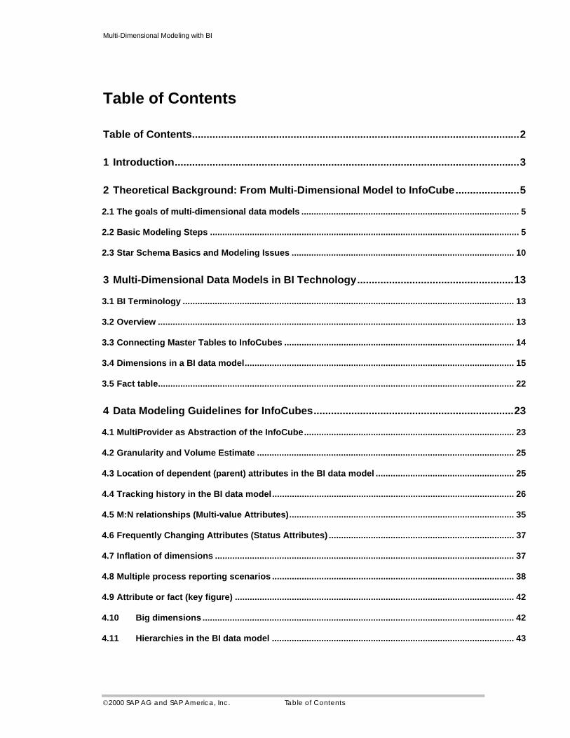
A simple example:
Sales Organisation Product Organisation Time KPIs
Sales Department Material Group Year Sales Amount
Sales Person Material Type Month Sales Quantity
Material Day
A multi-step multi-dimensional analysis will look like this:
1. Show me the Sales Amount by Sales Department by Material Group by Month 2. Show me the Sales Amount for a specific Sales Department ‘X’ by Material by Month
A DataStore object may serve to report on a single record (event) level such as:
Show yesterday’s Sales Orders for Sales Person ‘Y’.
This does not mean that sales order level data cannot reside in an InfoCube but rather that this is dependent upon particular information needs and navigation.
To summarize this simple example, two basic data modeling guidelines can be made:
Analytical processing (OLAP) is normally done using InfoCubes.
DataStore objects should not be misused for multi-dimensional analysis.
There are no hard and fast rules about the architecture of an enterprise data warehouse and this will not be discussed in any further detail here. It is important to bear in mind that this document deals only with the building of the Architected Data Mart layer with reusable BI Content objects, namely InfoCubes, with master data, and (external) hierarchies.
This document is organized the following way:
• In Chapter 2 this document provides initial information concerning the transition from an information need to the common multi-dimensional data model / Star schema. As the BI data model is based on the Star schema, an introduction to the Star schema will also be given and some general aspects explained.
Readers, who are familiar with the concepts of the multi-dimensional data model and the Star schema, may therefore want to skip this introducing Chapter 2.
• The BI data model is explained in detail in Chapter 3, where modeling aspects that are derived directly from the BI data model are also explained.
• Chapter 4 deals with several specific aspects in the BI data model (e.g. data modeling for time dependent analysis, hierarchical data) and further demands which might have to be designed with BI.
BI Data Modeling Guidelines within this document:
Important BI Data Modeling Guidelines within this document are always marked by shadowed text boxes.
Page 5
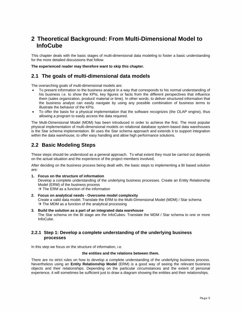
2 Theoretical Background: From Multi-Dimensional Model to InfoCube
This chapter deals with the basic stages of multi-dimensional data modeling to foster a basic understanding for the more detailed discussions that follow.
The experienced reader may therefore want to skip this chapter.
2.1 The goals of multi-dimensional data models
The overarching goals of multi-dimensional models are: • To present information to the business analyst in a way that corresponds to his normal understanding of
his business i.e. to show the KPIs, key figures or facts from the different perspectives that influence them (sales organization, product/ material or time). In other words, to deliver structured information that the business analyst can easily navigate by using any possible combination of business terms to illustrate the behavior of the KPIs.
• To offer the basis for a physical implementation that the software recognizes (the OLAP engine), thus allowing a program to easily access the data required.
The Multi-Dimensional Model (MDM) has been introduced in order to achieve the first. The most popular physical implementation of multi-dimensional models on relational database system-based data warehouses is the Star schema implementation. BI uses the Star schema approach and extends it to support integration within the data warehouse, to offer easy handling and allow high performance solutions.
2.2 Basic Modeling Steps
These steps should be understood as a general approach. To what extent they must be carried out depends on the actual situation and the experience of the project members involved.
After deciding on the business process being dealt with, the basic steps to implementing a BI based solution are:
1. Focus on the structure of information Develop a complete understanding of the underlying business processes. Create an Entity Relationship Model (ERM) of the business process
The ERM as a function of the information
2. Focus on analytical needs - Overcome model complexity Create a valid data model. Translate the ERM to the Multi-Dimensional Model (MDM) / Star schema
The MDM as a function of the analytical processing
3. Build the solution as a part of an integrated data warehouse The Star schema on the BI stage are the InfoCubes. Translate the MDM / Star schema to one or more InfoCube.
2.2.1 Step 1: Develop a complete understanding of the underlying business processes
In this step we focus on the structure of information, i.e.
the entities and the relations between them.
There are no strict rules on how to develop a complete understanding of the underlying business process. Nevertheless using an Entity Relationship Model (ERM) is a good way of seeing the relevant business objects and their relationships. Depending on the particular circumstances and the extent of personal experience, it will sometimes be sufficient just to draw a diagram showing the entities and their relationships.
Multi-Dimensional Modeling with BI
Page 6
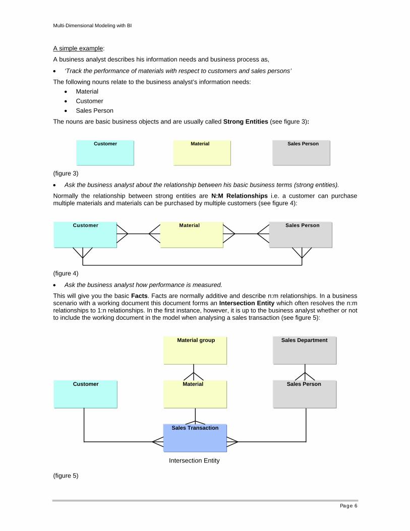
A simple example:
A business analyst describes his information needs and business process as,
• ‘Track the performance of materials with respect to customers and sales persons’
The following nouns relate to the business analyst’s information needs: • Material • Customer • Sales Person
The nouns are basic business objects and are usually called Strong Entities (see figure 3):
Customer Material Sales Person
(figure 3)
• Ask the business analyst about the relationship between his basic business terms (strong entities).
Normally the relationship between strong entities are N:M Relationships i.e. a customer can purchase multiple materials and materials can be purchased by multiple customers (see figure 4):
Customer Material Sales Person
(figure 4)
• Ask the business analyst how performance is measured.
This will give you the basic Facts. Facts are normally additive and describe n:m relationships. In a business scenario with a working document this document forms an Intersection Entity which often resolves the n:m relationships to 1:n relationships. In the first instance, however, it is up to the business analyst whether or not to include the working document in the model when analysing a sales transaction (see figure 5):
Customer
Sales Transaction
Material
Material group
Sales Person
Sales Department
Intersection Entity
(figure 5)
Multi-Dimensional Modeling with BI
Page 7
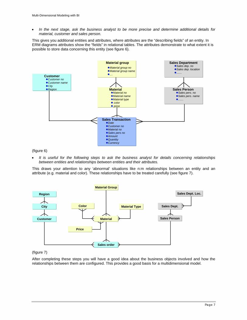
• In the next stage, ask the business analyst to be more precise and determine additional details for material, customer and sales person.
This gives you additional entities and attributes, where attributes are the “describing fields” of an entity. In ERM diagrams attributes show the “fields” in relational tables. The attributes demonstrate to what extent it is possible to store data concerning this entity (see figure 6).
Customer
Material Sales Person
Material group Sales Department
Customer noCustomer nameCityRegion
Material noMaterial nameMaterial type color price
Material group noMaterial group name....
Sales TransactionDateCustomer noMaterial noSales pers noAmountQuantityCurrency
Sales pers. noSales pers. name.......
Sales dep. noSales dep. location.......
(figure 6)
• It is useful for the following steps to ask the business analyst for details concerning relationships between entities and relationships between entities and their attributes.
This draws your attention to any ‘abnormal’ situations like n:m relationships between an entity and an attribute (e.g. material and color). These relationships have to be treated carefully (see figure 7).
Customer
City
Region
Material Group
Sales order
Price
Sales Person
Sales Dept.
Sales Dept. Loc.
Material
Material TypeColor
(figure 7)
After completing these steps you will have a good idea about the business objects involved and how the relationships between them are configured. This provides a good basis for a multidimensional model.
Multi-Dimensional Modeling with BI
Page 8
2.2.2 Step 2: Create a valid Data model
This crucial step aims to overcome model complexity by focusing on analytical needs. Overcoming model complexity involves the creation of a data model that is comprehensible for both the business analyst and the software.
2.2.2.1 The Multi-Dimensional Model (MDM)
Comprehensibility for the business analyst is reached by organizing entities and attributes from step 1 that are arranged in a parent-child relationship (1:N), into groups. These groups are called dimensions and the members of the dimensions dimension attributes, or attributes. The strong entities define the dimensions. For the business analyst the attributes of a dimension represent a specific business view on the facts (or key figures or KPIs), which are derived from the intersection entities. The attributes of a dimension are then organized in a hierarchical way and the most atomic attribute that forms the leaves of the hierarchy defines the granularity of the dimension. Granularity determines the detail of information. This model is called Multi-Dimensional Model (MDM). The Multi-Dimensional Model, where the facts are based in the center with the dimensions surrounding them, is a simple but effective concept that is easily recognized by technical resources as well as by the business analyst.
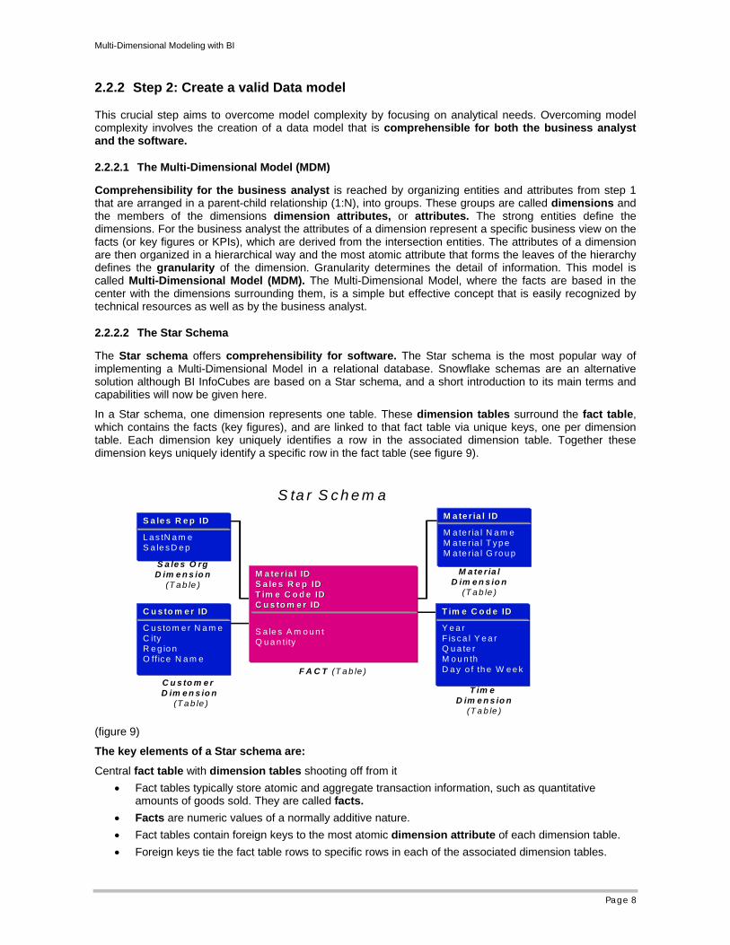
2.2.2.2 The Star Schema
The Star schema offers comprehensibility for software. The Star schema is the most popular way of implementing a Multi-Dimensional Model in a relational database. Snowflake schemas are an alternative solution although BI InfoCubes are based on a Star schema, and a short introduction to its main terms and capabilities will now be given here.
In a Star schema, one dimension represents one table. These dimension tables surround the fact table, which contains the facts (key figures), and are linked to that fact table via unique keys, one per dimension table. Each dimension key uniquely identifies a row in the associated dimension table. Together these dimension keys uniquely identify a specific row in the fact table (see figure 9).
S ta r S c h e m aS a le s R e pS a le s R e p ID ID
L a s tN a m eS a le s D e p
M a te r ia l IDM a te r ia l ID
M a te r ia l N a m eM a te r ia l T y p eM a te r ia l G ro u p
C u s to m e rC u s to m e r ID ID
C u s to m e r N a m eC ityR e g io nO ffic e N a m e
T im e C o d e IDT im e C o d e ID
Y e a rF is c a l Y e a rQ u a te rM o u n thD a y o f th e W e e k
M a te r ia l IDM a te r ia l IDS a le s R e pS a le s R e p ID IDT im e C o d e IDT im e C o d e IDC u s to m e rC u s to m e r ID ID
S a le s A m o u n tQ u a n tity
T im e D im e n s io n
(T a b le )
C u s to m e r D im e n s io n
(T a b le )
S a le s O rg D im e n s io n
(T a b le )M a te r ia l
D im e n s io n (T a b le )
F A C T (T a b le )
(figure 9)
The key elements of a Star schema are:
Central fact table with dimension tables shooting off from it • Fact tables typically store atomic and aggregate transaction information, such as quantitative
amounts of goods sold. They are called facts. • Facts are numeric values of a normally additive nature. • Fact tables contain foreign keys to the most atomic dimension attribute of each dimension table. • Foreign keys tie the fact table rows to specific rows in each of the associated dimension tables.
Multi-Dimensional Modeling with BI
Page 9
• The points of the star are dimension tables. • Dimension tables store both attributes about the data stored in the fact table and textual data. • Dimension tables are de-normalized. • The most atomic dimension attributes in the dimensions define the granularity of the information,
i.e. the number of records in the fact table.
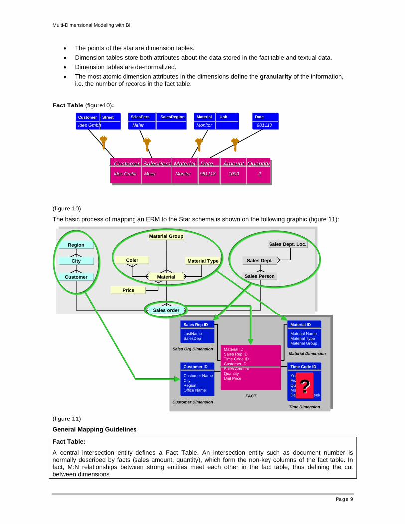
Fact Table (figure10):
CustomerCustomer StreetStreet SalesPersSalesPers SalesRegionSalesRegion MaterialMaterial UnitUnit DateDateDate
Customer SalesPers Material Date Amount QuantityIdes Gmbh Meier Monitor 981118 1000 2
Customer SalesPers Material Date Amount QuantityIdes Gmbh Meier Monitor 981118 1000 2
Ides Gmbh Meier Monitor 981118
(figure 10)
The basic process of mapping an ERM to the Star schema is shown on the following graphic (figure 11):
Sales Rep ID
LastNameSalesDep
Material ID
Material NameMaterial TypeMaterial Group
Customer ID
Customer NameCityRegionOffice Name
Time Code ID
YearFiscal YearQuaterMounthDay of the Week
Material IDSales Rep IDTime Code IDCustomer IDSales AmountQuantityUnit Price
Time DimensionCustomer Dimension
Sales Org DimensionMaterial Dimension
FACT??
Customer
City
Region
Material Group
Sales order
Price
Sales Person
Sales Dept.
Sales Dept. Loc.
Material
Material TypeColor
(figure 11)
General Mapping Guidelines
Fact Table:
A central intersection entity defines a Fact Table. An intersection entity such as document number is normally described by facts (sales amount, quantity), which form the non-key columns of the fact table. In fact, M:N relationships between strong entities meet each other in the fact table, thus defining the cut between dimensions
Multi-Dimensional Modeling with BI
Page 10
Dimensions (Tables):
Attributes with 1:N conditional relationships should be stored in the same dimension such as material group and material.
The foreign primary key relations define the dimensions
Time:
One exception is the time dimension. As there is no correspondence in the ERM, time attributes (day, week, year) have to be introduced in the MDM process to cover the analysis needs.
These considerations provide a starting point for dimension analysis, but additional considerations will impact on the grouping of the attributes and will be discussed in detail later.
2.2.3 Step 3: Create an InfoCube Description
Translating the MDM / Star schema (i.e. the results of Step 1 and Step 2) into an InfoCube description is of course the topic of this paper and will be investigated in the following chapters 3 and 4 in depth. The next section 2.3 discusses basic facts and modeling issues of the Star schema in general.
2.3 Star Schema Basics and Modeling Issues
In the previous section we introduced the Star schema. As most of the relevant properties for modeling derive directly from these schemas, we will now have a closer look to them. We start with the Star schema as it is the force behind the BI schema (i.e. the InfoCube) and is also easier to understand. These basics will also help you to develop a fundamental understanding of the modeling properties of the BI schema before that is discussed in the next chapter.
We emphasize that this chapter discusses the Star schema and not the BI data model (InfoCube)
2.3.1 How The Star Schema Works
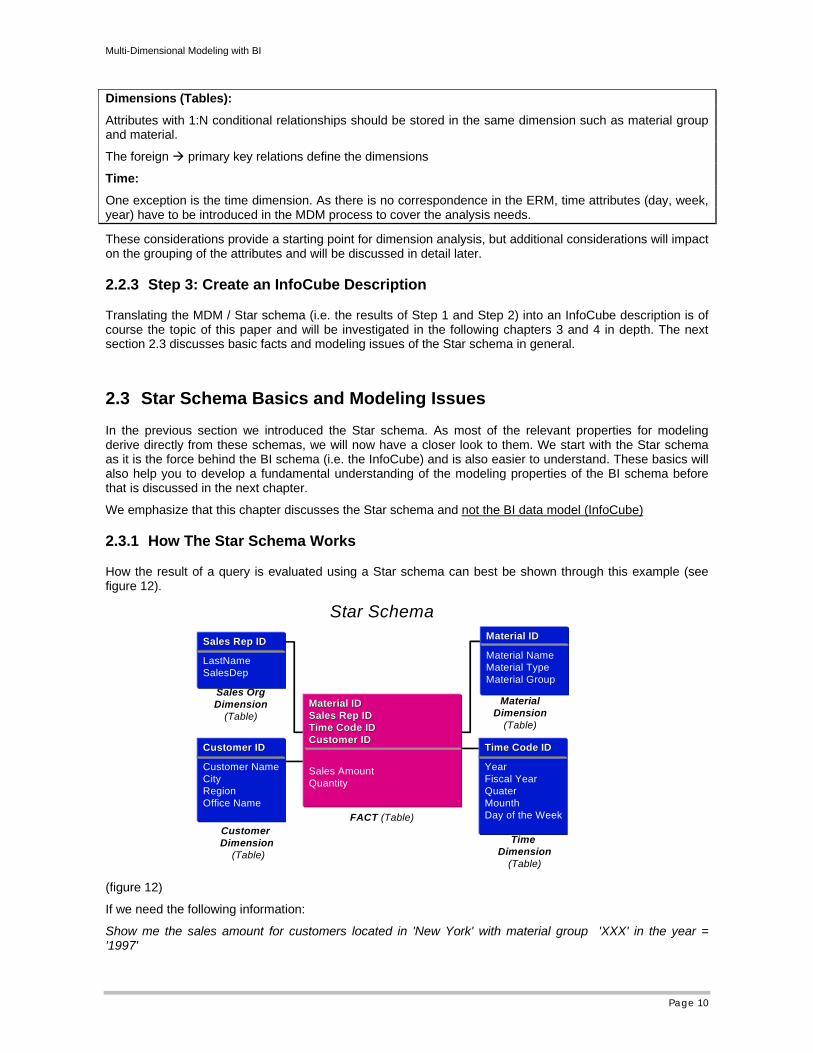
How the result of a query is evaluated using a Star schema can best be shown through this example (see figure 12).
Star SchemaSales RepSales Rep ID ID
LastNameSalesDep
Material IDMaterial ID
Material NameMaterial TypeMaterial Group
CustomerCustomer ID ID
Customer NameCityRegionOffice Name
Time Code IDTime Code ID
YearFiscal YearQuaterMounthDay of the Week
Material IDMaterial IDSales RepSales Rep ID IDTime Code IDTime Code IDCustomerCustomer ID ID
Sales AmountQuantity
Time Dimension
(Table)
Customer Dimension
(Table)
Sales Org Dimension
(Table)Material
Dimension (Table)
FACT (Table)
(figure 12)
If we need the following information:
Show me the sales amount for customers located in 'New York' with material group 'XXX' in the year = '1997'
Multi-Dimensional Modeling with BI
Page 11
The answer is determined in two stages:
1. Browsing the Dimension Tables
• Access the Customer Dimension Table and select all records with City = 'New York'
• Access the Material Dimension Table and select all records with Material group = 'XXX'
• Access the Time Dimension Table and select all records with Year = '1997'
• As a result of these three browsing activities, there are a number of key values (Customer IDs, Material IDs, Time Code ID), one from each dimension table affected.
2. Accessing the Fact Table
Using the key values evaluated during browsing, select all records in the fact table that have these values in common in the fact table record key.
2.3.2 Star Schema Issues
With respect to the processing of a query and the design of the Star schema we realize that:
Reflecting ‘real world’ changes in the Star schema
How real-world changes are dealt with, i.e. how the different time aspects are handled is the most important topic with data warehouses.
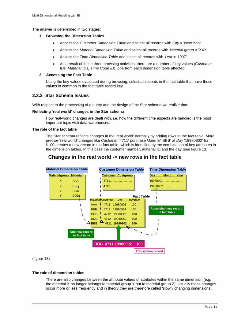
The role of the fact table
The Star schema reflects changes in the ‘real world’ normally by adding rows to the fact table. More precise ‘real world’ changes like Customer ‘4711’ purchase Material ‘BBB’ at Day ‘19980802’ for $100 creates a new record in the fact table, which is identified by the combination of key attributes in the dimension tables. In this case the customer number, material ID and the day (see figure 13):
Changes in the real world -> new rows in the fact table
Materialgroup Material
X AAA
X BBB Y CCC Y DDD
Materialgroup Material
X AAA
X BBB Y CCC Y DDD
Material Customer Day Revenue
AAA 4711 19980901 100 BBB 4712 19980901 100 CCC 4712 19980901 100 DDD 4712 19980901 100 BBB 4711 19980902 100
Material Customer Day Revenue
AAA 4711 19980901 100 BBB 4712 19980901 100 CCC 4712 19980901 100 DDD 4712 19980901 100 BBB 4711 19980902 100
Material Dimension Table
Fact Table
BBB 4711 19980902 100
Transaction record
Add new record to fact table
Customer Custgroup
4711...........................
4712...........................
Customer Custgroup
4711...........................
4712...........................
Day Month Year
19980901 .....................
19980902 .....................
Day Month Year
19980901 .....................
19980902 .....................
Customer Dimension Table Time Dimension Table
Accessing new record in fact table
(figure 13)
The role of dimension tables
There are also changes between the attribute values of attributes within the same dimension (e.g. the material X no longer belongs to material group Y but to material group Z). Usually these changes occur more or less frequently and in theory they are therefore called ‘slowly changing dimensions’.
Multi-Dimensional Modeling with BI
Page 12
How these changes are dealt with has a big impact on reporting possibilities and data warehouse management. The different possible time scenarios and how to solve these within BI are discussed in detail in the next sections.
Reporting
• Queries can be created by accessing the dimension tables (master data reporting).
• The Star schema saves information about events that did or did not happen (e.g. reporting the revenue for the customers in New York within a certain time span would show the customers that have revenue, but not the customers that have no revenue).
Aggregation
• Only the information at the granularity of the dimension table keys (material ID, customer ID, time code ID, sales rep ID) need to be stored to make any desired aggregated level of information available.
• More precisely: any summarized information can be retrieved at run time i.e. as far as functionality is concerned, there is no need to store pre-calculated aggregated data, but with large ( number of rows) fact tables and / or large dimension tables, pre-calculated aggregates must be introduced for performance reasons.
Attribute Relationships (Hierarchies)
In the Star schema there is one (real) attribute (most granular) as the unique identifier of each dimension table row joining the fact table. The other attributes of a dimension table are normally ‘parents’ of such identifying attributes, thus the term hierarchy. With hierarchies numerous challenges must be resolved:
• N:M relationship within a dimension.
There is no simple way to handle an N:M relationship between two attributes within a dimension table (such as materials with different colors). If material is the lowest level, it is not possible to put both material and material color into one normal star dimension table, as we would have one material value associated with multiple colors. As such, material is no longer a unique key.
• No leaf attribute values.
Again there is no easy way to handle transactional input to a Star schema where the facts are offered at different attribute levels, whereby the attributes belong to the same dimension. For example, assume the attributes material and material group exist in the same dimension. Some subsidiaries can offer transactional data at material level whereas others can only offer data at material group level. The result in the latter case is dimension table rows with blank or null values for the material, which destroys the unique key material.
• Unbalanced hierarchies
Very often we have attributes in a dimension where a relationship exists between some attribute values, whereas with others there is none. As the relations between attribute values of different attributes within a dimension form a tree that will result in paths of differing lengths from root to leaves, these unbalanced hierarchies will produce reports with dummy hierarchy tree nodes.
Table Sizes and Performance
Do not destroy browsing performance. Dimension tables should have a 'relatively' small number of rows (in comparison to the fact table; factor at least 1:10 to 1:20).
Schema Maintenance
• There are no limitations to the Star schema with respect to the number of attributes in the dimension and fact tables, except the limitations caused by the underlying relational database.
• Flexibility regarding the addition of characteristics and key figures to the schema is caused by properties of relational databases.
Multi-Dimensional Modeling with BI
Page 13
3 Multi-Dimensional Data Models in BI Technology Based on experience with the Star schema, the BI data model (InfoCube) uses a more sophisticated approach to guarantee consistency in the data warehouse and to offer data model-based functionality to cover the business analyst’s reporting needs.
Creating a valid multi-dimensional data model in BI means that you always have to bear in mind the overall enterprise data warehouse requirements and the solution-specific analysis and reporting needs. Errors in this area will have a deep impact on the solution, resulting in poor performance or even an invalid data model.
3.1 BI Terminology
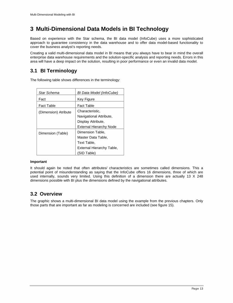
The following table shows differences in the terminology:
Star Schema BI Data Model (InfoCube)
Fact Key Figure
Fact Table Fact Table
(Dimension) Atribute Characteristic, Navigational Attribute, Display Attribute, External Hierarchy Node
Dimension (Table) Dimension Table, Master Data Table, Text Table, External Hierarchy Table, (SID Table)
Important
It should again be noted that often attributes/ characteristics are sometimes called dimensions. This a potential point of misunderstanding as saying that the InfoCube offers 16 dimensions, three of which are used internally, sounds very limited. Using this definition of a dimension there are actually 13 X 248 dimensions possible with BI plus the dimensions defined by the navigational attributes.
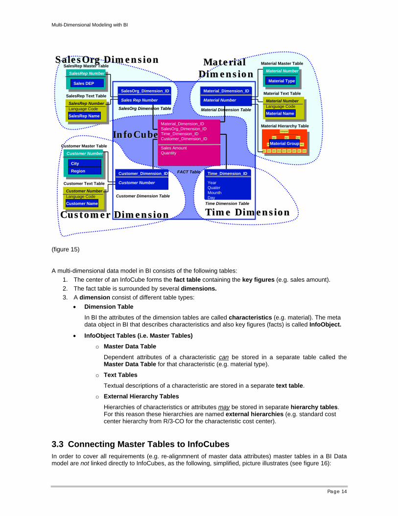
3.2 Overview The graphic shows a multi-dimensional BI data model using the example from the previous chapters. Only those parts that are important as far as modeling is concerned are included (see figure 15).
Multi-Dimensional Modeling with BI
Page 14
FACT Table
Gebiet 1 Gebiet 2 Gebiet 3
Bezirk 1
Gebiet 3a
Bezirk 2
Region 1
Gebiet 4 Gebiet 5
Bezirk 3
Region 2
Gebiet 6
Bezirk 4
Gebiet 7 Gebiet 8
Bezirk 5
Region 3
Vertriebsorganisation
Material Group
Material Hierarchy TableMaterial_Dimension_IDSalesOrg_Dimension_IDTime_Dimension_IDCustomer_Dimension_ID
Sales AmountQuantity
Material NumberLanguage Code
Material NumberLanguage Code
Material Name
Material Text TableMaterial_Dimension_ID
Material Number
Material Dimension Table
Material Master Table
Material NumberMaterial Number
Material Type
SalesRep Master Table
SalesRep NumberSalesRep Number
Sales DEP
SalesRep NumberLanguage Code
SalesRep NumberLanguage Code
SalesRep Name
SalesRep Text Table
Customer NumberLanguage Code
Customer NumberLanguage Code
Customer Name
Customer Text Table
Customer Master Table
Customer NumberCustomer Number
City
Region Time_Dimension_ID
YearQuaterMounthDay
Time Dimension Table
SalesOrg_Dimension_ID
Sales Rep Number
SalesOrgSalesOrg Dimension Dimension TableTable
Customer_Dimension_ID
Customer Number
Customer Dimension Table
Cus tom e r Cus tom e r Dim e n s ionDim e n s ion
In foCubeIn foCube
Tim eTim e Dim e n s ion Dim e n s ion
Mate rialMate rial Dim e ns ion Dim e n s ion
Sale s OrgSale s Org Dim e ns ion Dim e n s ion
(figure 15)
A multi-dimensional data model in BI consists of the following tables: 1. The center of an InfoCube forms the fact table containing the key figures (e.g. sales amount). 2. The fact table is surrounded by several dimensions. 3. A dimension consist of different table types:
• Dimension Table
In BI the attributes of the dimension tables are called characteristics (e.g. material). The meta data object in BI that describes characteristics and also key figures (facts) is called InfoObject.
• InfoObject Tables (i.e. Master Tables)
o Master Data Table
Dependent attributes of a characteristic can be stored in a separate table called the Master Data Table for that characteristic (e.g. material type).
o Text Tables
Textual descriptions of a characteristic are stored in a separate text table.
o External Hierarchy Tables
Hierarchies of characteristics or attributes may be stored in separate hierarchy tables. For this reason these hierarchies are named external hierarchies (e.g. standard cost center hierarchy from R/3-CO for the characteristic cost center).
3.3 Connecting Master Tables to InfoCubes In order to cover all requirements (e.g. re-alignmnent of master data attributes) master tables in a BI Data model are not linked directly to InfoCubes, as the following, simplified, picture illustrates (see figure 16):
Multi-Dimensional Modeling with BI
Page 15
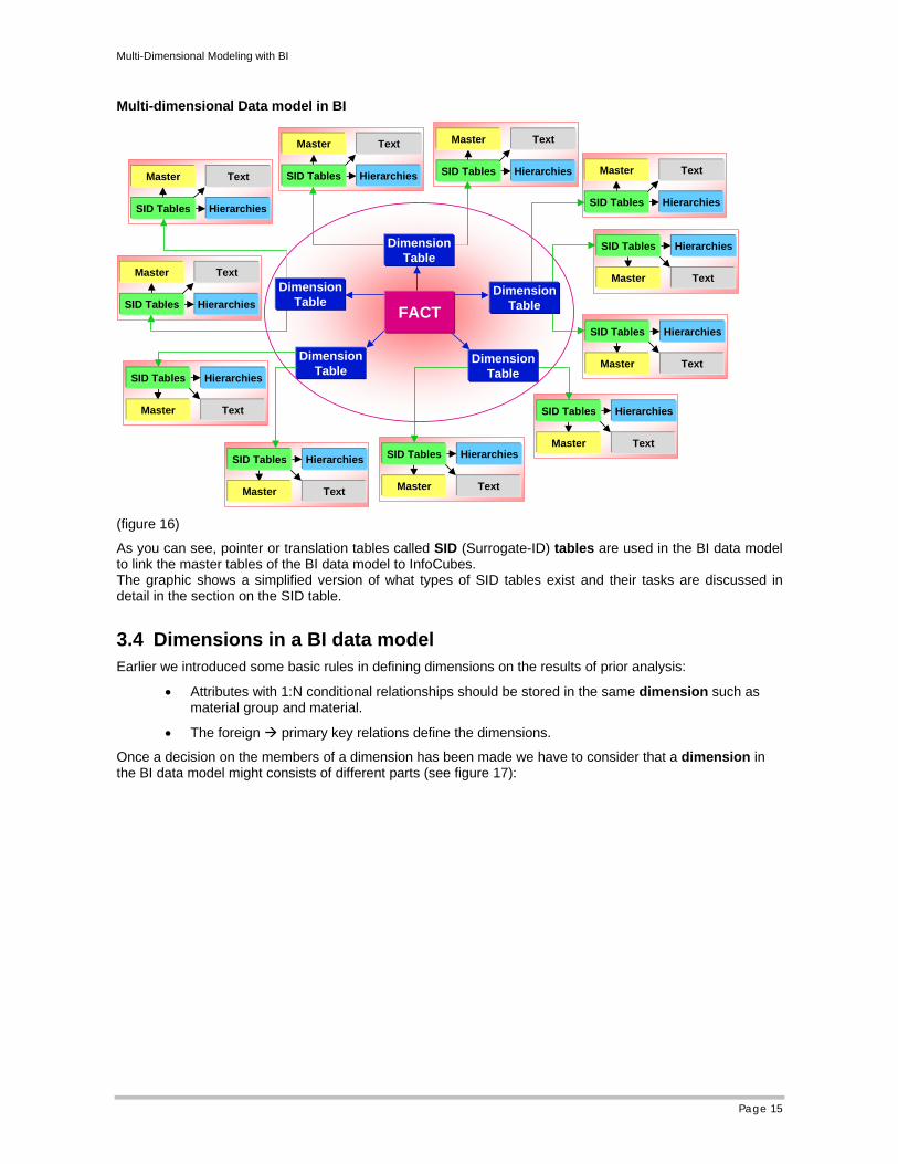
Multi-dimensional Data model in BI
Text
SID Tables
Master
Hierarchies
Hierarchies
Master
SID Tables
Text
Hierarchies
Master
SID Tables
Text
Hierarchies
Master
SID Tables
Text
Hierarchies
Master
SID Tables
Text
Hierarchies
Master
SID Tables
Text
Text
SID Tables
Master
Hierarchies
Text
SID Tables
Master
Hierarchies
Text
SID Tables
Master
Hierarchies
DimensionTable
Text
SID Tables
Master
Hierarchies
DimensionTable
DimensionTable
DimensionTable
DimensionTable
Hierarchies
Master
SID Tables
Text
FACT
(figure 16)
As you can see, pointer or translation tables called SID (Surrogate-ID) tables are used in the BI data model to link the master tables of the BI data model to InfoCubes. The graphic shows a simplified version of what types of SID tables exist and their tasks are discussed in detail in the section on the SID table.
3.4 Dimensions in a BI data model Earlier we introduced some basic rules in defining dimensions on the results of prior analysis:
• Attributes with 1:N conditional relationships should be stored in the same dimension such as material group and material.
• The foreign primary key relations define the dimensions.
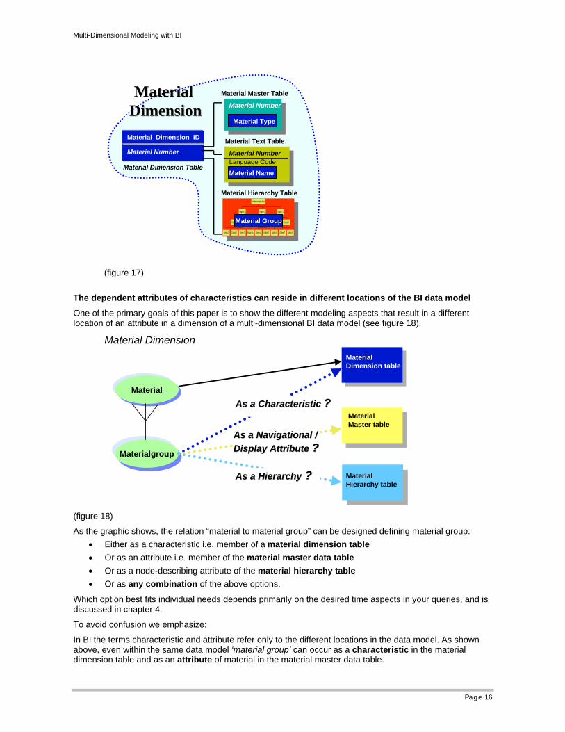
Once a decision on the members of a dimension has been made we have to consider that a dimension in the BI data model might consists of different parts (see figure 17):
Multi-Dimensional Modeling with BI
Page 16
Gebiet 1 Gebiet 2 Gebiet 3
Bezirk 1
Gebiet 3a
Bezirk 2
Region 1
Gebiet 4 Gebiet 5
Bezirk 3
Region 2
Gebiet 6
Bezirk 4
Gebiet 7 Gebiet 8
Bezirk 5
Region 3
Vertriebsorganisation
Material Group
Material Hierarchy Table
Material NumberLanguage Code
Material NumberLanguage Code
Material Name
Material Text TableMaterial_Dimension_ID
Material Number
Material Dimension Table
Material Master Table
Material NumberMaterial Number
Material Type
MaterialMaterial Dimension Dimension
(figure 17)
The dependent attributes of characteristics can reside in different locations of the BI data model
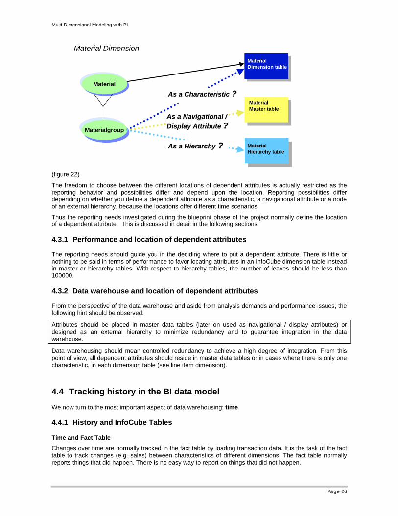
One of the primary goals of this paper is to show the different modeling aspects that result in a different location of an attribute in a dimension of a multi-dimensional BI data model (see figure 18).
Material
Material Dimension
Materialgroup
MaterialDimension table
As a Characteristic As a Characteristic ?? MaterialMaster table
As a NavigationalAs a Navigational / /DisplayDisplay Attribute Attribute ??
MaterialHierarchy table
As a HierarchyAs a Hierarchy ? ?
(figure 18)
As the graphic shows, the relation “material to material group” can be designed defining material group: • Either as a characteristic i.e. member of a material dimension table • Or as an attribute i.e. member of the material master data table • Or as a node-describing attribute of the material hierarchy table • Or as any combination of the above options.
Which option best fits individual needs depends primarily on the desired time aspects in your queries, and is discussed in chapter 4.
To avoid confusion we emphasize:
In BI the terms characteristic and attribute refer only to the different locations in the data model. As shown above, even within the same data model ‘material group’ can occur as a characteristic in the material dimension table and as an attribute of material in the material master data table.
Multi-Dimensional Modeling with BI
Page 17
3.4.1 Master Data Table
The attributes of a characteristic that will reside in its master data table are determined in the modeling phase. Each attribute can be defined individually as being time dependent:
• There is one ‘time dependent’ check box for each attribute in the ‘attribute’ tab page section.
• Time dependency of an attribute allows you to keep track on the changes over time of the relation of the characteristic and the time dependent attribute values.
• In terms of technical implementation, two master data tables exist if we have both non-time dependent and time dependent attributes.
o One master data table stores all relations to non-time dependent attributes (name of the table: /BIC/P<InfoObject name>) and
o One table stores relations to time dependent attributes (name of the table: /BIC/Q<InfoObject name>).
• The time dependent attributes master data table has additional DATETO and DATEFROM system attributes. In queries the different constellations are addressed using the key date ( Query properties). The validity attributes are not available for navigation.
3.4.2 Text Table
The text table of an InfoObject of type characteristic keeps the descriptions of the characteristic values. The existence of a text table and different description types as short, middle and long text descriptions and language dependency can be defined in the master data tab page section.
The text table, or better the description attributes, may be defined as time dependent.
3.4.3 SID Tables
SID tables play an important role in linking the data warehouse information structures to the InfoCubes and DataStore Objects. To speed up access to InfoCubes and DataStore Objects and to allow an independent master data layers, each characteristic and attribute is assigned a SID column and their values are encoded into 4-byte integer values.
3.4.3.1 InfoObject definition and SID tables
To offer optimal performance with the various data models with respect to master data access, three different SID tables might be generated.
SID tables with respect to master data:
• The SID table is always generated if an InfoObject is not defined as ‘attribute only’ (tab page general). This table is used if the access to an Infocube or DataStore Object uses a navigational attribute or if the access is via a characteristic without attributes. Name of the table: /BIC/S<InfoObject name>
• The non-time dependent attribute SID table of a characteristic for access via non-time dependent attributes. Name of the table: /BIC/X<InfoObject name>
• The time dependent attribute SID table of a characteristic for access via time dependent attributes. Name of the table: /BIC/Y<InfoObject name>
All these SID tables are automatically maintained during master data load. SID tables are also maintained during InfoCube load if no referential integrity check is enforced (InfoPackage).
Example:
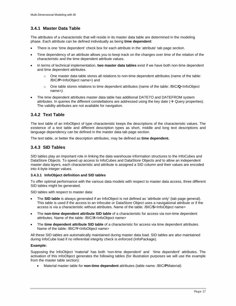
Supposing the InfoObject ‘material’ has both ‘non-time dependent’ and ‘time dependent’ attributes. The activation of this InfoObject generates the following tables (for illustration purposes we will use the example from the master table section):
• Material master table for non-time dependent attributes (table name: /BIC/PMaterial)
Multi-Dimensional Modeling with BI
Page 18
Material Material Type AAA 100 BBB 200 CCC 100 DDD 100
• Material master table for time dependent attributes (table name: /BIC/QMaterial)
Material Date from Date to Material Group AAA 01/1000 12/9999 X BBB 01/1000 09/2005 X BBB 10/2005 12/9999 Y CCC 01/1000 12/9999 Y DDD 01/1000 12/9999 Y
• Material SID table (table name: /BIC/SMaterial)
Material SID Material 001 AAA 002 BBB 003 CCC 004 DDD
• Material non-time dependent attribute SID table (table name: /BIC/XMaterial)
Material SID Material Mat.Type SID001 AAA 22222 002 BBB 33333 003 CCC 22222 004 DDD 22222
• Material time dependent attribute SID table (table name: /BIC/YMaterial)
Material SID Material Date from Date to Mat.Group SID 001 AAA 01/1000 12/9999 910 002 BBB 01/1000 09/2005 910 002 BBB 10/2005 12/9999 920 003 CCC 01/1000 12/9999 920 004 DDD 01/1000 12/9999 920
3.4.3.2 InfoCube Access and SID Tables
To get an understanding of the function of these SID tables a simple example is given as to how the result of a query is evaluated. If we need the following information:
Show me the sales amount for customers located in 'New York' with material group 'X' and ‘Y’ in the year = '1999'
Let us assume that the material group is a navigational attribute (non-time dependent) of the characteristic material in the material master data table and we have no predefined aggregates at material group level.
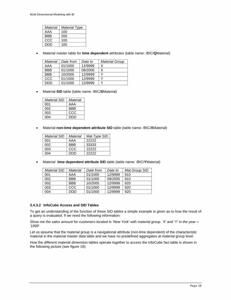
How the different material dimension tables operate together to access the InfoCube fact table is shown in the following picture (see figure 19):
Multi-Dimensional Modeling with BI
Page 19
1 1 2 2 3 3
111 111 222 222 333 333
Dim ID SID Material
Fact table Dimension table
Material not time dependent Attributes SID table (Name: /BIC/XMATERIAL)
Material Non-time Attributes SID table (Name: /BIC/XMATERIAL)
Material MatGroup AAA CCC DDD
X Y Y
Material Master table (Name: /BIC/PMATERIAL)
Material Master table (Name: /BIC/PMATERIAL)
1 1 2 2 3 3
10.000 12.000 25.000
Dim ID Sales
SID Material Material SID MatGroup
AAA CCC DDD
111 111 222 222 333 333
345345678678678678
MatGroup SID MatGroup
X Y Z
345 678 999 MatGroup SID table
(Name: /BIC/SMATGROUP)MatGroup SID table (Name: /BIC/SMATGROUP)Not used for Infocube access !
Example: Show me the sales values for material group X
Not used in this Example :•Traditional Material SID Table: /BIC/SMATERIAL •Time dependent Material Master Table: /BIC/Q MATERIAL •Material Time dependent Attributes SID Table: /BIC/Y MATERIAL
Not used in this Example :•Traditional Material SID Table: /BIC/SMATERIAL •Time dependent Material Master Table: /BIC/Q MATERIAL •Material Time dependent Attributes SID Table: /BIC/Y MATERIAL
SID Tables for Infocube Access
(figure 19)
The result set for the material groups is then determined in two steps:
1. Browsing the tables that form the dimensions
• Material dimension
Access the material group SID table and select the material group SIDs (here ‘345’ and ‘678’) for material group = 'X' and ‘Y’
Access the material non-time dependent attribute SID table with these material group SIDs and determine the material SID values (here ‘111’, ‘222’ and ‘333’).
Access the material dimension table with these material SID values and determine the material dimension table Dim-Id values (here ‘1’, ‘2’ and ‘3’)
• Customer dimension: same proceeding
• Time dimension: same proceeding
As a result of these three browsing activities, there are a number of key values (material dimension table DIM-IDs, customer dimension table DIM-IDs, time dimension table DIM-IDs), one from each dimension table affected.
2. Accessing the fact table
Using the key values (DIM-IDs) determined during browsing, select all records in the fact table that have these values in the fact table record key.
We can summarize that in accessing an InfoCube no ‘real value’ master data tables are used.
3.4.4 External Hierarchy Table
In general hierarchies are structures essential to navigation. Having characteristics and attributes in dimension tables and master data tables that are related in a sequence of parent-child relationships indicates, of course, not only hierarchies, but internal hierarchies.
Multi-Dimensional Modeling with BI
Page 20
The external hierarchies of a characteristic are defined separately from the other master data and, as mentioned above, are independent of specific InfoCubes. They are therefore called external hierarchies. The different model properties of ‘internal’ and ‘external’ hierarchies in the BI Data model will be discussed in chapter 4.
During the creation of an InfoObject of type characteristic you can define the basic functionality of external hierarchies for this InfoObject (Tab page: ‘hierarchies’) or whether they will exist at all.
3.4.4.1 Tables for external hierarchies
The activation of the InfoObject ‘material’ results in the creation of the following tables: • Material hierarchy table: /BIC/HMaterial • Material hierarchy SID table: /BIC/KMaterial • Material SID-structure hierarchy table: /BIC/IMaterial
3.4.4.2 External hierarchies and InfoCube access
BI allows you to determine multiple external hierarchies for a characteristic. External hierarchies can be used for characteristics in the dimension tables and for activated navigational attributes for query navigation.
Example:
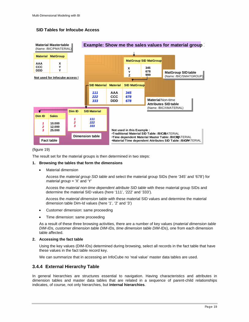
Consider a simple external hierarchy for the characteristic ‘country’. ‘Country’ is a member of the customer dimension table but it could instead, or additionally, be a navigational attribute in the customer master data table. The nodes are of a textual nature. See figure 20.
World
Europe
Germany Austria Switzerland
America
USA Canada
Japan
-3
-2
3 4 5
-1
1 2
6*
Country Hierarchy
* Set Ids only shown for better understanding (figure 20)
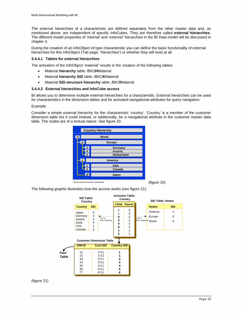
The following graphic illustrates how the access works (see figure 21):
SID Table: Nodes
Nodes
America
Europe
World
SID
-1
-2
-3
Child
-2-1 66 33 4 4 55 11 2 2
Parent
-3-3-3-2-2-2-1-1
Inclusion Table: Country
SID
6 3 4 5 1 2
SID Table: Country
Country
JapanGermanyAustriaSwitz.USACanada
Customer Dimension TableDIM-ID
11223344556677
Cust-SID
1711171227113711471157116711
Country-SID
11112233445566
Text & Rep. Attributes
Text & Rep. Attributes
FactTable
(figure 21)
Multi-Dimensional Modeling with BI
Page 21
A node of a hierarchy can either be textual or it can be an InfoObject with a specified value e.g. InfoObject ‘material group’ with value ‘X’. All display attributes of the InfoObject ‘material group’ are associated with this node.
The use of InfoCube-independent hierarchy tables is an additional prerequisite for an enterprise-wide data warehouse as the hierarchy table for a characteristic only exists once. Multiple InfoCubes sharing the same characteristic in a dimension table access the same hierarchy table. This is another architectural aspect that accommodates data integration.
3.4.5 Dimension tables of an InfoCube
3.4.5.1 Defining dimension tables
In defining an InfoCube you select all the InfoObjects of type characteristic that will be direct members of this InfoCube. After this you define your dimensions and assign the selected characteristics to a dimension.
Important
BI does not force you to only assign related characteristics to the same dimension table, offering you additional data model potential. Nevertheless, as a basic rule you should only put characteristics that have a parent-child relationship in the same dimension.
The activation of the InfoCube then results (with one exception which we will discuss later) in the generation of an InfoCube dimension table for each dimension.
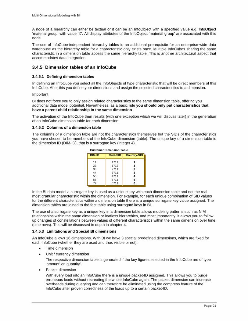
3.4.5.2 Columns of a dimension table
The columns of a dimension table are not the characteristics themselves but the SIDs of the characteristics you have chosen to be members of the InfoCube dimension (table). The unique key of a dimension table is the dimension ID (DIM-ID), that is a surrogate key (integer 4).
Customer Dimension TableDIM-ID
11223344556677
Cust-SID
1711171227113711471157116711
Country-SID
11112233445566
In the BI data model a surrogate key is used as a unique key with each dimension table and not the real most granular characteristic within the dimension. For example, for each unique combination of SID values for the different characteristics within a dimension table there is a unique surrogate key value assigned. The dimension tables are joined to the fact table using surrogate keys in BI.
The use of a surrogate key as a unique key in a dimension table allows modeling patterns such as N:M relationships within the same dimension or leafless hierarchies, and most importantly, it allows you to follow up changes of constellations between values of different characteristics within the same dimension over time (time rows). This will be discussed in depth in chapter 4.
3.4.5.3 Limitations and Special BI dimensions
An InfoCube allows 16 dimensions. With BI we have 3 special predefined dimensions, which are fixed for each InfoCube (whether they are used and thus visible or not):
• Time dimension • Unit / currency dimension
The respective dimension table is generated if the key figures selected in the InfoCube are of type ‘amount’ or ‘quantity’.
• Packet dimension With every load into an InfoCube there is a unique packet-ID assigned. This allows you to purge erroneous loads without recreating the whole InfoCube again. The packet dimension can increase overheads during querying and can therefore be eliminated using the compress feature of the InfoCube after proven correctness of the loads up to a certain packet-ID.
Multi-Dimensional Modeling with BI
Page 22
The remaining 13 dimensions are for individual data model design
Each dimension table may be up to 248 characteristics.
It should again be noted that generally attributes/ characteristics are sometimes called dimensions. This a potential point of misunderstanding as saying that the InfoCube offers 16 dimensions, three of which are used internally, sounds very limited. Using this definition of a dimension there are actually 13 X 248 dimensions possible with BI plus the dimensions defined by the navigational attributes.
3.4.5.4 Dimensions and navigation
All characteristics assigned to dimension tables can be used for navigation (drilling) and filtering within queries. Navigation with navigational attributes of InfoCube characteristics has to be explicitly switched on for each navigational attribute (Tab page: ‘navigation’). The activation of a navigational attribute for an InfoCube can be done afterwards. Deactivation of navigational attributes is not possible!
3.4.5.5 Dimensions with only one characteristic (line item dimensions)
It is very often possible in this model to assign only one characteristic to a dimension.This will probably occur with specific reporting requirements or if for example you have the document line item in your model.
In these situations a dimension table means only overhead. BI allows you define this kind of dimension as a line item dimension (Check box dimension definition). In doing this no dimension table will be generated for this dimension. As dimension table will serve the SID table of this characteristic. The key in the fact table will be the SID of the SID Table.
3.5 Fact table
The fact table is created during InfoCube activation. The structure of the fact table in the BI data model is the same as it is in the normal Star schema. The keys of the dimension tables (i.e. the DIM-IDs) or the SIDs of line item dimensions are the foreign keys in the fact table. The non-key columns are defined by the selected key figures during InfoCube definition.
• Each row in the fact table is uniquely identified by a value combination of the respective DIM-IDs / SIDs of the dimension / SID tables
• Since the BI uses system-assigned surrogate keys, namely DIM-IDs or SIDs of 4 bytes in length per dimension to link the dimension / SID tables to the fact table, there will normally be a decrease in space requirements for keys in comparison to the use of real characteristic values for keys.
• The dimension / master (SID) tables should be relatively small with respect to the number of rows in comparison to the fact table (factor 1:10 / 20).
Multiple Fact Tables
Each InfoCube has two fact tables:
The F-fact table, which is optimized for loading data, and the E-fact table, which is optimized for retrieving data. Both fact tables have the same columns. The F-fact table uses b-tree indexes, whereas the E-fact table uses bitmap indexes except for line item dimensions where a b-tree index is used.
The InfoCube compression feature moves the fact records of all selected requests from the F- to the E-fact table. In doing so the request-ID of each fact record is set to zero.
The separation into two fact tables is fully transparent.
Multi-Dimensional Modeling with BI
Page 23
4 Data Modeling Guidelines for InfoCubes We will now look at the various important BI data modeling guidelines from a topic-based perspective. Explaining how to implement these issues with BI will improve understanding of the BI data model.
InfoCubes Define the Physical Database Tables
Activating an InfoCube in the Data Warhousing Workbench results in the creation of physical data base tables. Each dimension defines a dimension table and the key-figures the fact-table(s) of the BI extended star-schema.
The order we add the various key-figures during an InfoCube defintion will exactly be the order of the columns in the fact-table(s). It is therefore a good modeling solution to add first the key figures, which are always filled and then key figures, which are rarely filled as this would support the compression of the data base as we find it with Oracle. This is especially important with high volume scenarios.
4.1 MultiProvider as Abstraction of the InfoCube
The InfoCube results directly in the creation of physical database tables. This has certain issues:
• Reduced flexibility, if we have to change the InfoCube later
• Reduced modeling flexibility
As described in chapter 2 the analysis of the business requirements results finally in a logical multidimensional model where the key figures are surrounded by dimensionally grouped characteristics/ navigational attributes. All the characteristics/ navigational attributes of a dimension have normally a hierarchical relation. Accepting these grouping 1:1 for an InfoCube dimension may result in unacceptable large dimension tables:
• e.g. we have a logical dimension with order-no and item-no. with expected 1 million orders and 5 items on an average per order we would have an InfoCube dimension table with 5 million entries. This is not clever.
• Instead we could define 2 InfoCube dimensions: one for order one for item resulting in an order dimension with 1 million records and an item dimension with 5 records.
• Defining an MultiProvider on top of this InfoCube would allow to regroup order-no and item-no into a single dimension.

Multi-Dimensional Modeling with BI
Page 24
It is straightforward to define queries directly on an InfoCube, but this will significantly reduce flexibility. If for whatever reason the InfoCube has to be redesigned later the queries and the related reports are directly affected. This illustrates the following picture:
We therefore recommend always to define queries on MultiProviders, which serve as a buffer to the InfoCube.
Multi-Dimensional Modeling with BI
Page 25
4.2 Granularity and Volume Estimate
An important result of the data modeling phase is that the granularity (the level of detail of your data) is determined. Granularity deeply influences
• Reporting capabilities • Performance • Data volume • Load Time
You have to decide whether you really need to store detailed data in an InfoCube or whether it is better in an DataStore object or even not stored in your data warehouse at all, but accessed directly from your Source system via drill thru.
Fact tables and granularity
Volume is a concern with fact tables. Large fact tables impact on reporting and analysis performance. How can the number of rows of data in a fact table be estimated? Consider the following:
• How long will the data be stored in the fact table?
• How granular will the data be?
The first is fairly straightforward. However, the granularity of the information has a large impact on querying efficiency and overall storage requirements. The granularity of the fact table is directly impacted by dimension table design as the most atomic characteristic in each dimension determines the granularity of the fact table.
Simple example Let us assume we need to analyze the performance of outlets and articles. We further assume that 1,000 articles are grouped by 10 article groups. To track the article group performance on a weekly basis:
• Granularity: article group, week, and 300 sales days a year (45 weeks)
10 X 45 = 450 records in the fact table per year due to only these two attributes if all articles are sold within a week.
• Granularity: article, week, 300 sales days a year (45 weeks)
1,000 X 45 = 45,000 records in the fact table per year due to only these two attributes if all articles are sold within a week.
• Granularity: article, day, 300 sales days a year
1,000 X 300 = 300,000 records in the fact table per year due to only these two attributes if all articles are sold within a day.
• Granularity: article, hour, 300 sales days a year, 12 sales hours a day
500 X 300 X 12 = 1,800,000 records in the fact table per year due to only these two attributes if on average 500 articles are sold within an hour.
Finally, assuming 500 outlets, there will be 900,000,000 records a year in the fact table.
4.3 Location of dependent (parent) attributes in the BI data model
The BI data model offers more than one possible location for dependent attributes. Where to put dependent attributes in the BI data model is one of the decisive results of the projects blueprint phase and is mainly influenced how to reflect changes in the parent/chield relationship over time. (See section “Slowly changing dimensions”)
Multi-Dimensional Modeling with BI
Page 26
Material
Material Dimension
Materialgroup
MaterialDimension table
As a Characteristic As a Characteristic ?? MaterialMaster table
As a NavigationalAs a Navigational / /DisplayDisplay Attribute Attribute ??
MaterialHierarchy table
As a HierarchyAs a Hierarchy ? ?
(figure 22)
The freedom to choose between the different locations of dependent attributes is actually restricted as the reporting behavior and possibilities differ and depend upon the location. Reporting possibilities differ depending on whether you define a dependent attribute as a characteristic, a navigational attribute or a node of an external hierarchy, because the locations offer different time scenarios.
Thus the reporting needs investigated during the blueprint phase of the project normally define the location of a dependent attribute. This is discussed in detail in the following sections.
4.3.1 Performance and location of dependent attributes
The reporting needs should guide you in the deciding where to put a dependent attribute. There is little or nothing to be said in terms of performance to favor locating attributes in an InfoCube dimension table instead in master or hierarchy tables. With respect to hierarchy tables, the number of leaves should be less than 100000.
4.3.2 Data warehouse and location of dependent attributes
From the perspective of the data warehouse and aside from analysis demands and performance issues, the following hint should be observed:
Attributes should be placed in master data tables (later on used as navigational / display attributes) or designed as an external hierarchy to minimize redundancy and to guarantee integration in the data warehouse.
Data warehousing should mean controlled redundancy to achieve a high degree of integration. From this point of view, all dependent attributes should reside in master data tables or in cases where there is only one characteristic, in each dimension table (see line item dimension).
4.4 Tracking history in the BI data model
We now turn to the most important aspect of data warehousing: time
4.4.1 History and InfoCube Tables
Time and Fact Table
Changes over time are normally tracked in the fact table by loading transaction data. It is the task of the fact table to track changes (e.g. sales) between characteristics of different dimensions. The fact table normally reports things that did happen. There is no easy way to report on things that did not happen.
Multi-Dimensional Modeling with BI
Page 27
Simple example:
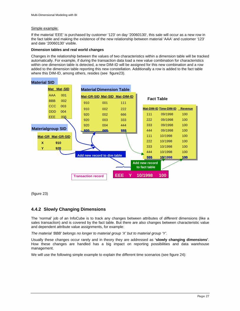
If the material ‘EEE‘ is purchased by customer ‘123‘ on day ‘20060130‘, this sale will occur as a new row in the fact table and making the existence of the new relationship between material ‘AAA‘ and customer ‘123‘ and date ‘20060130’ visible.
Dimension tables and real world changes
Changes in the relationship between the values of two characteristics within a dimension table will be tracked automatically. For example, if during the transaction data load a new value combination for characteristics within one dimension table is detected, a new DIM-ID will be assigned for this new combination and a row added to the dimension table reporting this new constellation. Additionally a row is added to the fact table where this DIM-ID, among others, resides (see figure23).
(figure 23)
4.4.2 Slowly Changing Dimensions
The ‘normal’ job of an InfoCube is to track any changes between attributes of different dimensions (like a sales transaction) and is covered by the fact table. But there are also changes between characteristic value and dependent attribute value assignments, for example:
The material ‘BBB’ belongs no longer to material group ‘X’ but to material group ‘Y’.
Usually these changes occur rarely and in theory they are addressed as ‘slowly changing dimensions’. How these changes are handled has a big impact on reporting possibilities and data warehouse management.
We will use the following simple example to explain the different time scenarios (see figure 24):
Fact Table
Mat -GR-SID Mat-SID Mat-DIM-ID
910 001 111
910 002 222
920 002 666 920 003 333 920 004 444
920 005 555
Mat -GR-SID Mat-SID Mat-DIM-ID
910 001 111
910 002 222 920 002 666 920 003 333 920 004 444
920 005 555920 005 555
Mat Mat -SID
AAA 001 BBB 002 CCC 003 DDD 004 EEE 005
Mat -GR Mat -GR-SID
X 910 Y 920
Mat-DIM-ID Time-DIM-ID Revenue
111 09/1998 100 222 09/1998 100 333 09/1998 100 444 09/1998 100 111 10/1998 100 222 10/1998 100 333 10/1998 100 444 10/1998 100 555 10/1998 100
Mat-DIM-ID Time-DIM-ID Revenue 111 09/1998 100 222 09/1998 100 333 09/1998 100 444 09/1998 100 111 10/1998 100 222 10/1998 100 333 10/1998 100 444 10/1998 100 555 555 10/ 10/1998 100 100
Material Dimension Table
Fact Table
EEE Y 10/1998 100Transaction record
Add new record to dim table
Add new record to fact table
Material SID
Materialgroup SID
Multi-Dimensional Modeling with BI
Page 28
Constellation 09/1998:
Material Material group
AAA X BBB X CCC Y DDD Y
Constellation 10/1998:
Material Material group
AAA X BBB Y (changed) CCC Y DDD Y EEE Y (new)
Material Date Revenue
AAA 09/1998 100 BBB 09/1998 100 CCC 09/1998 100 DDD 09/1998 100
AAA 10/1998 100 BBB 10/1998 100 CCC 10/1998 100 DDD 10/1998 100 EEE 10/1998 100
Fact Table
(figure 24)
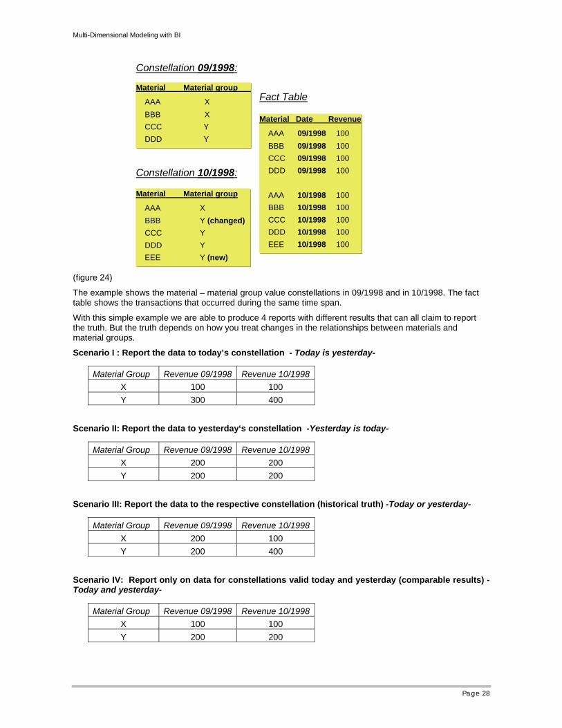
The example shows the material – material group value constellations in 09/1998 and in 10/1998. The fact table shows the transactions that occurred during the same time span.
With this simple example we are able to produce 4 reports with different results that can all claim to report the truth. But the truth depends on how you treat changes in the relationships between materials and material groups.
Scenario I : Report the data to today’s constellation - Today is yesterday-
Scenario II: Report the data to yesterday‘s constellation -Yesterday is today-
Scenario III: Report the data to the respective constellation (historical truth) -Today or yesterday-
Scenario IV: Report only on data for constellations valid today and yesterday (comparable results) -Today and yesterday-
Material Group Revenue 09/1998 Revenue 10/1998X 100 100 Y 300 400
Material Group Revenue 09/1998 Revenue 10/1998X 200 200 Y 200 200
Material Group Revenue 09/1998 Revenue 10/1998X 200 100 Y 200 400
Material Group Revenue 09/1998 Revenue 10/1998X 100 100 Y 200 200
Multi-Dimensional Modeling with BI
Page 29
4.4.2.1 Scenario I: Report the data to today’s constellation - today is yesterday
Description:
Report all fact data according to today’s value constellation of a characteristic and a dependent attribute.
See simple example above:
In 10/1998 the assignment of material ‘BBB’ to material group ‘X’ was changed to ‘Y’. A new material ‘EEE’ assigned to material group ‘Y’ appeared. You are not interested in the old assignments anymore. Thus you report on the fact data as if material ‘BBB’ belonged to material group ‘Y’ from the very beginning.
Example from reality:
This time scenario typically occurs with sales forces. When the assignment of sales persons to customers changes to a new sales person-customer constellation, all the sales data from earlier times will be reported as if they always referred to the new sales person. This requirement means a realignment of the fact data to the new constellation.
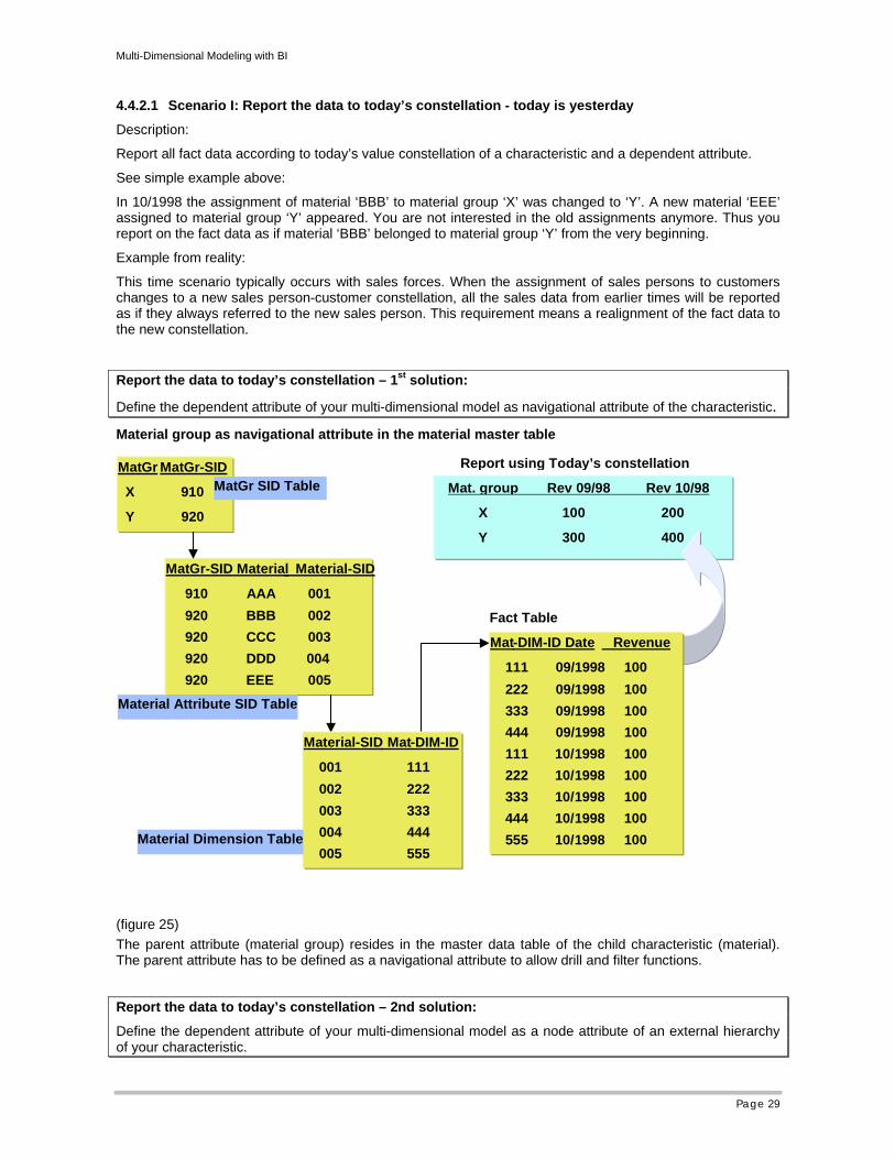
Report the data to today’s constellation – 1st solution:
Define the dependent attribute of your multi-dimensional model as navigational attribute of the characteristic.
Material group as navigational attribute in the material master table
Fact Table
MatGr MatGr-SID
X 910
Y 920
MatGr SID Table
MatGr-SID Material Material-SID
910 AAA 001 920 BBB 002 920 CCC 003 920 DDD 004 920 EEE 005
Material-SID Mat-DIM-ID
001 111 002 222 003 333 004 444 005 555
Material Dimension Table
Mat-DIM-ID Date Revenue
111 09/1998 100 222 09/1998 100 333 09/1998 100 444 09/1998 100 111 10/1998 100 222 10/1998 100 333 10/1998 100 444 10/1998 100 555 10/1998 100
Material Attribute SID Table
Report using Today’s constellation
Mat. group Rev 09/98 Rev 10/98
X 100 200
Y 300 400
(figure 25) The parent attribute (material group) resides in the master data table of the child characteristic (material). The parent attribute has to be defined as a navigational attribute to allow drill and filter functions.
Report the data to today’s constellation – 2nd solution:
Define the dependent attribute of your multi-dimensional model as a node attribute of an external hierarchy of your characteristic.
Multi-Dimensional Modeling with BI
Page 30
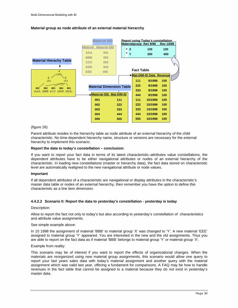
Material group as node attribute of an external material hierarchy
Materialgroup Rev 9/98 Rev 10/98
X 100 100 Y 300 400
Report using Today‘s constallation
Mat-DIM-ID Date Revenue
111 9/1998 100 222 9/1998 100 333 9/1998 100 444 9/1998 100 111 10/1998 100 222 10/1998 100 333 10/1998 100 444 10/1998 100 555 10/1998 100
Fact Table
Material Material-SID
AAA 001 BBB 002 CCC 003 DDD 004 EEE 005
Material SID
Material-SID Mat-DIM-ID
001 111 002 222 003 333 004 444 005 555
Material Dimension Table
Material Hierachy Table
-1(All)
-2(X)
-3(Y)
001(AAA)
002(BBB)
003(CCC)
004(DDD)
005(EEE)
++
(figure 26)
Parent attribute resides in the hierarchy table as node attribute of an external hierarchy of the child characteristic. No time-dependent hierarchy name, structure or versions are necessary for the external hierarchy to implement this scenario.
Report the data to today’s constellation – conclusion:
If you want to report your fact data in terms of its latest characteristic–attributes value constellations, the dependent attributes have to be either navigational attributes or nodes of an external hierarchy of the characteristic. In loading new constellations (master or hierarchy data), the fact data stored on characteristic level are automatically realigned to the new navigational attribute or node values.
Important
If all dependent attributes of a characteristic are navigational or display attributes in the characteristic’s master data table or nodes of an external hierarchy, then remember you have the option to define this characteristic as a line item dimension.
4.4.2.2 Scenario II: Report the data to yesterday’s constellation - yesterday is today
Description:
Allow to report the fact not only to today’s but also according to yesterday’s constellation of characteristics and attribute value assignments.
See simple example above:
In 10 1998 the assignment of material ‘BBB’ to material group ‘X’ was changed to ‘Y’. A new material ‘EEE’ assigned to material group ‘Y’ appeared. You are interested in the new and the old assignments. Thus you are able to report on the fact data as if material ‘BBB’ belongs to material group ‘Y’ or material group ‘X’.
Example from reality:
This scenario may be of interest if you want to report the effects of organizational changes. When the materials are reorganized using new material group assignments, this scenario would allow one query to report your last years sales data with today’s material assignment and another query with the material assignment which was valid last year, offering a fundament for comparisons. A FAQ may be how to handle revenues in the fact table that cannot be assigned to a material because they do not exist in yesterday’s master data.
Multi-Dimensional Modeling with BI
Page 31
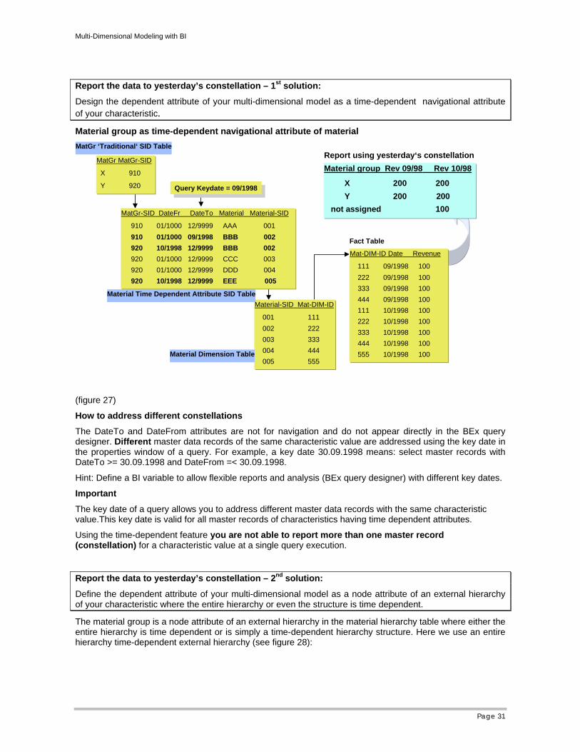
Report the data to yesterday’s constellation – 1st solution:
Design the dependent attribute of your multi-dimensional model as a time-dependent navigational attribute of your characteristic.
Material group as time-dependent navigational attribute of material
Fact Table
MatGr MatGr-SID
X 910
Y 920
MatGr ‘Traditional‘ SID Table
Material-SID Mat-DIM-ID
001 111 002 222 003 333 004 444 005 555
Material Dimension Table
Mat-DIM-ID Date Revenue
111 09/1998 100 222 09/1998 100 333 09/1998 100 444 09/1998 100 111 10/1998 100 222 10/1998 100 333 10/1998 100 444 10/1998 100 555 10/1998 100
Material Time Dependent Attribute SID Table
MatGr-SID DateFr DateTo Material Material-SID
910 01/1000 12/9999 AAA 001 910 01/1000 09/1998 BBB 002 920 10/1998 12/9999 BBB 002 920 01/1000 12/9999 CCC 003 920 01/1000 12/9999 DDD 004 920 10/1998 12/9999 EEE 005
Material group Rev 09/98 Rev 10/98
X 200 200 Y 200 200 not assigned 100
Report using yesterday‘s constellation
Query Keydate = 09/1998Query Keydate = 09/1998
(figure 27)
How to address different constellations
The DateTo and DateFrom attributes are not for navigation and do not appear directly in the BEx query designer. Different master data records of the same characteristic value are addressed using the key date in the properties window of a query. For example, a key date 30.09.1998 means: select master records with DateTo >= 30.09.1998 and DateFrom =< 30.09.1998.
Hint: Define a BI variable to allow flexible reports and analysis (BEx query designer) with different key dates.
Important
The key date of a query allows you to address different master data records with the same characteristic value.This key date is valid for all master records of characteristics having time dependent attributes.
Using the time-dependent feature you are not able to report more than one master record (constellation) for a characteristic value at a single query execution.
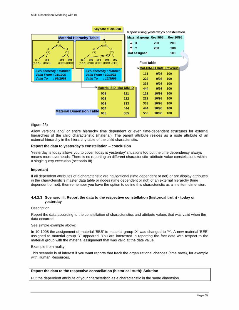
Report the data to yesterday’s constellation – 2nd solution:
Define the dependent attribute of your multi-dimensional model as a node attribute of an external hierarchy of your characteristic where the entire hierarchy or even the structure is time dependent.
The material group is a node attribute of an external hierarchy in the material hierarchy table where either the entire hierarchy is time dependent or is simply a time-dependent hierarchy structure. Here we use an entire hierarchy time-dependent external hierarchy (see figure 28):
Multi-Dimensional Modeling with BI
Page 32
Mat-DIM-ID Date Revenue
111 9/98 100 222 9/98 100 333 9/98 100 444 9/98 100 111 10/98 100 222 10/98 100 333 10/98 100 444 10/98 100 555 10/98 100
Mat-DIM-ID Date Revenue
111 9/98 100 222 9/98 100 333 9/98 100 444 9/98 100 111 10/98 100 222 10/98 100 333 10/98 100 444 10/98 100 555 10/98 100
Fact table
Material-SID Mat-DIM-ID
001 111 002 222 003 333 004 444 005 555
Material-SID Mat-DIM-ID
001 111 002 222 003 333 004 444 005 555Material Dimension Table
Material Hierachy Table Material group Rev 9/98 Rev 10/98
X 200 200 Y 200 200 not assigned 100
Report using yesterday‘s constellation
++
-1(All)
-2(X)
-3(Y)
001(AAA)
002(BBB)
003(CCC)
004(DDD)
005(EEE)
-1 (All)
-2 (X)
-3 (Y)
001(AAA)
002(BBB)
003(CCC)
004(DDD)
Ext Hierarchy : MathierValid From : 01/1000Valid To : 09/1998
Ext Hierarchy : MathierValid From : 10/1998Valid To : 12/9999
Keydate = 09/1998Keydate = 09/1998
(figure 28)
Allow versions and/ or entire hierarchy time dependent or even time-dependent structures for external hierarchies of the child characteristic (material). The parent attribute resides as a node attribute of an external hierarchy in the hierarchy table of the child characteristic.
Report the data to yesterday’s constellation – conclusion
Yesterday is today allows you to cover 'today is yesterday' situations too but the time dependency always means more overheads. There is no reporting on different characteristic–attribute value constellations within a single query execution (scenario III).
Important
If all dependent attributes of a characteristic are navigational (time dependent or not) or are display attributes in the characteristic’s master data table or nodes (time dependent or not) of an external hierarchy (time dependent or not), then remember you have the option to define this characteristic as a line item dimension.
4.4.2.3 Scenario III: Report the data to the respective constellation (historical truth) - today or yesterday
Description
Report the data according to the constellation of characteristics and attribute values that was valid when the data occurred.
See simple example above:
In 10 1998 the assignment of material ‘BBB’ to material group ‘X’ was changed to ‘Y’. A new material ‘EEE’ assigned to material group ‘Y’ appeared. You are interested in reporting the fact data with respect to the material group with the material assignment that was valid at the date value.
Example from reality:
This scenario is of interest if you want reports that track the organizational changes (time rows), for example with Human Resources.
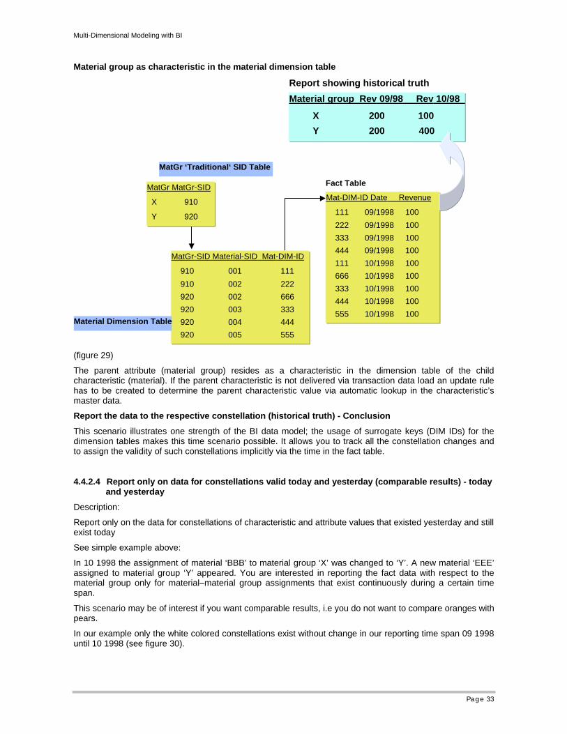
Report the data to the respective constellation (historical truth): Solution
Put the dependent attribute of your characteristic as a characteristic in the same dimension.
Multi-Dimensional Modeling with BI
Page 33
Material group as characteristic in the material dimension table
Fact TableMatGr MatGr-SID
X 910
Y 920
MatGr ‘Traditional‘ SID Table
MatGr-SID Material-SID Mat-DIM-ID
910 001 111 910 002 222 920 002 666 920 003 333 920 004 444 920 005 555
Material Dimension Table
Mat-DIM-ID Date Revenue
111 09/1998 100 222 09/1998 100 333 09/1998 100 444 09/1998 100 111 10/1998 100 666 10/1998 100 333 10/1998 100 444 10/1998 100 555 10/1998 100
Material group Rev 09/98 Rev 10/98
X 200 100 Y 200 400
Report showing historical truth
(figure 29)
The parent attribute (material group) resides as a characteristic in the dimension table of the child characteristic (material). If the parent characteristic is not delivered via transaction data load an update rule has to be created to determine the parent characteristic value via automatic lookup in the characteristic’s master data.
Report the data to the respective constellation (historical truth) - Conclusion
This scenario illustrates one strength of the BI data model; the usage of surrogate keys (DIM IDs) for the dimension tables makes this time scenario possible. It allows you to track all the constellation changes and to assign the validity of such constellations implicitly via the time in the fact table.
4.4.2.4 Report only on data for constellations valid today and yesterday (comparable results) - today and yesterday
Description:
Report only on the data for constellations of characteristic and attribute values that existed yesterday and still exist today
See simple example above:
In 10 1998 the assignment of material ‘BBB’ to material group ‘X’ was changed to ‘Y’. A new material ‘EEE’ assigned to material group ‘Y’ appeared. You are interested in reporting the fact data with respect to the material group only for material–material group assignments that exist continuously during a certain time span.
This scenario may be of interest if you want comparable results, i.e you do not want to compare oranges with pears.
In our example only the white colored constellations exist without change in our reporting time span 09 1998 until 10 1998 (see figure 30).
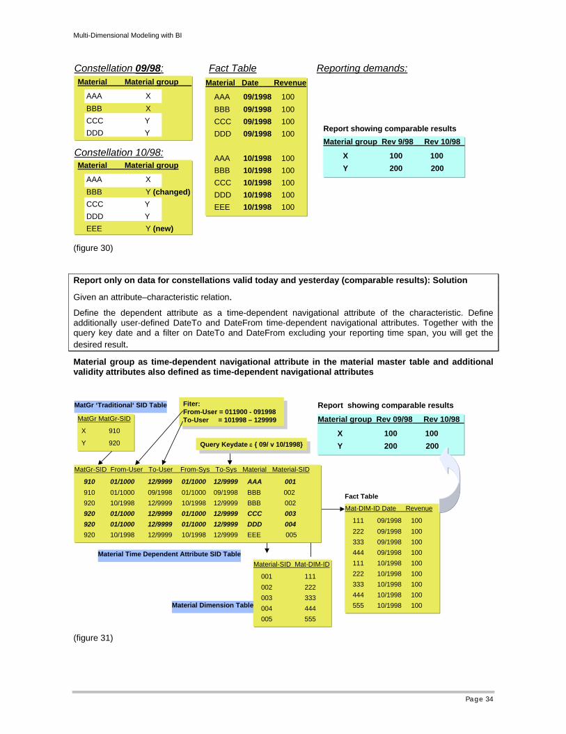
Multi-Dimensional Modeling with BI
Page 34
Constellation 09/98:Material Material group
AAA X BBB X CCC Y DDD Y
Constellation 10/98:Material Material group
AAA X BBB Y (changed) CCC Y DDD Y EEE Y (new)
Reporting demands:Fact Table
Material group Rev 9/98 Rev 10/98
X 100 100 Y 200 200
Report showing comparable results
Material Date Revenue
AAA 09/1998 100 BBB 09/1998 100 CCC 09/1998 100 DDD 09/1998 100
AAA 10/1998 100 BBB 10/1998 100 CCC 10/1998 100 DDD 10/1998 100 EEE 10/1998 100
(figure 30)
Report only on data for constellations valid today and yesterday (comparable results): Solution
Given an attribute–characteristic relation. Define the dependent attribute as a time-dependent navigational attribute of the characteristic. Define additionally user-defined DateTo and DateFrom time-dependent navigational attributes. Together with the query key date and a filter on DateTo and DateFrom excluding your reporting time span, you will get the desired result.
Material group as time-dependent navigational attribute in the material master table and additional validity attributes also defined as time-dependent navigational attributes
Fact Table
MatGr MatGr-SID
X 910
Y 920
MatGr ‘Traditional‘ SID Table
Material-SID Mat-DIM-ID
001 111 002 222 003 333 004 444 005 555
Material Dimension Table
Mat-DIM-ID Date Revenue
111 09/1998 100 222 09/1998 100 333 09/1998 100 444 09/1998 100 111 10/1998 100 222 10/1998 100 333 10/1998 100 444 10/1998 100 555 10/1998 100
Material Time Dependent Attribute SID Table
Query Keydate ε { 09/ v 10/1998}Query Keydate ε { 09/ v 10/1998}
MatGr-SID From-User To-User From-Sys To-Sys Material Material-SID
910 01/1000 12/9999 01/1000 12/9999 AAA 001 910 01/1000 09/1998 01/1000 09/1998 BBB 002 920 10/1998 12/9999 10/1998 12/9999 BBB 002 920 01/1000 12/9999 01/1000 12/9999 CCC 003 920 01/1000 12/9999 01/1000 12/9999 DDD 004 920 10/1998 12/9999 10/1998 12/9999 EEE 005
Material group Rev 09/98 Rev 10/98
X 100 100 Y 200 200
Report showing comparable resultsFiter:From-User = 011900 - 091998To-User = 101998 – 129999
Fiter:From-User = 011900 - 091998To-User = 101998 – 129999
(figure 31)
Multi-Dimensional Modeling with BI
Page 35
• As in the ‘yesterday is today’ scenario we store all the different parent-child constellations that have occurred over time.
• The parent attribute (material group) resides in the master data table of the child characteristic. • The key date mechanism for addressing specific master data records does not allow time ranges. • Furthermore the DateTo and DateFrom (To-Sys/From-Sys) attributes that are generated
automatically to handle time-dependent attributes cannot be used for-user defined navigation or filters.
• You have to define your own DateTo and DateFrom attributes (To-User and From-User) in the master table.
• During master data load the user DateTo value of the old master record has to be updated. • Hint: Define time variables with intervals for DateFrom and DateTo to allow flexible reports and
analysis (BEx Query Designer). • For example, to make a query with comparable data for the period 9/1998 to 10/1998 you have to
define the intervals as follows:
(userdefined) DateFrom: 011900 - 091998
(userdefined) DateTo: 101998 – 129999
The query key date must be in 9 or 10/1998
4.4.3 Usage of time scenarios (Guidelines for BI Data Modeling)
As shown in the previous section BI supports a wide range of time scenarios. Summarizing what we learned in the previous sections we emphasize:
It is possible to incorporate each time scenario within one BI data model.
Using different time scenarios in a data model increases the potential value of our solution.
It is understandable that the business analyst may wish to have all the time scenarios in the BI data model – just in case. If this is so but there is no fundamental justification for this in terms of information needs, the business analyst should be warned that he will pay for it in the following ways:
He will lose the simplicity of the Multi-Dimensional Model and moreover produce extra overheads during loading and querying:
• With each additional time scenario in a BI data model the complexity is increased and with it, the potential of erroneous and misleading queries. Additional training has to be done for ad hoc users and for query authors to explain the differences between the time scenarios and how and in which cases to use them.
• The value of the historical structure diminishes with time, especially with scenario II.
• Scenarios I & III are by far the most frequently used scenarios.
• When designing the same parent attribute as a characteristic in a dimension table (scenario III: historical truth) and as an navigational attribute in a master data table (all other scenarios) remember that in a BI data model the navigational attribute should have a different name from its name in the InfoObject definition to avoid misunderstandings. Otherwise the same name would be repeated twice in the BEx Query Designer.
4.5 M:N relationships (Multi-value Attributes)
M:N relationships detected during logical modeling need special observation.
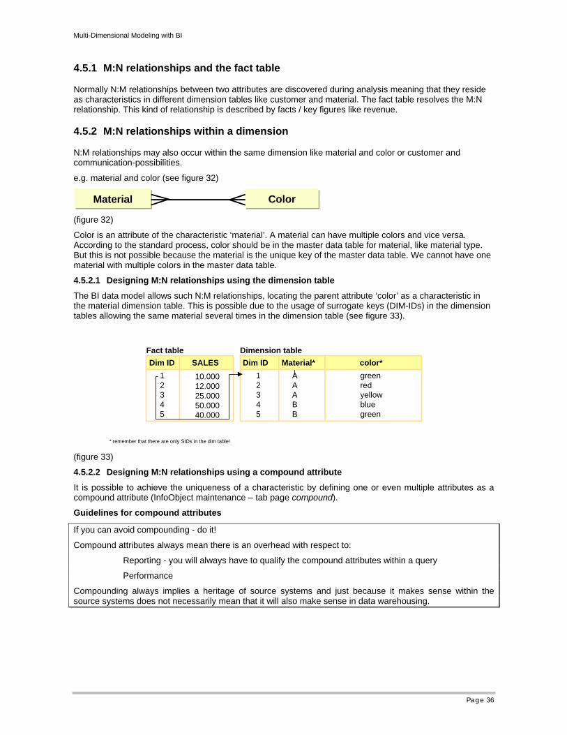
Multi-Dimensional Modeling with BI
Page 36
4.5.1 M:N relationships and the fact table
Normally N:M relationships between two attributes are discovered during analysis meaning that they reside as characteristics in different dimension tables like customer and material. The fact table resolves the M:N relationship. This kind of relationship is described by facts / key figures like revenue.
4.5.2 M:N relationships within a dimension
N:M relationships may also occur within the same dimension like material and color or customer and communication-possibilities.
e.g. material and color (see figure 32)
Material Color
(figure 32)
Color is an attribute of the characteristic ‘material’. A material can have multiple colors and vice versa. According to the standard process, color should be in the master data table for material, like material type. But this is not possible because the material is the unique key of the master data table. We cannot have one material with multiple colors in the master data table.
4.5.2.1 Designing M:N relationships using the dimension table
The BI data model allows such N:M relationships, locating the parent attribute ‘color’ as a characteristic in the material dimension table. This is possible due to the usage of surrogate keys (DIM-IDs) in the dimension tables allowing the same material several times in the dimension table (see figure 33).
AAABB
Dim ID Umsatz Dim ID Material* color*12345
10.00012.00025.00050.00040.000
Fact table Dimension tableDim ID SALES
greenredyellowbluegreen
* remember that there are only SIDs in the dim table!
12345
(figure 33)
4.5.2.2 Designing M:N relationships using a compound attribute
It is possible to achieve the uniqueness of a characteristic by defining one or even multiple attributes as a compound attribute (InfoObject maintenance – tab page compound).
Guidelines for compound attributes
If you can avoid compounding - do it!
Compound attributes always mean there is an overhead with respect to:
Reporting - you will always have to qualify the compound attributes within a query
Performance
Compounding always implies a heritage of source systems and just because it makes sense within the source systems does not necessarily mean that it will also make sense in data warehousing.
Multi-Dimensional Modeling with BI
Page 37
4.6 Frequently Changing Attributes (Status Attributes)
If you find frequently changing characteristic–attribute relations in your data model then the master data table is not normally the right place to handle these relation as:
• Defining the attribute as time-dependent would result in an explosion of the master data, which is not efficient.
• More importantly: you normally want to report on the effects of these changes but a time-dependent attribute only allows you to report on one constellation at a time (query execution).
• Furthermore very often such an attribute is not only dependent on time and one other characteristic but on a combination of characteristics.
Simple example:
Promotion Status
The promotion status is an attribute of ‘article’. The promotion values could be TV, newspaper, or handouts. Being the nature of status attributes, the status of an article changes frequently. The promotion status is normally not only an attribute of article but a combination of article and outlet: e.g. an article may be on promotion in one outlet whereas it is not on promotion for others.
This leads to:
Frequently changing attributes should be designed as a characteristic of their own dimension table.
Regarding our simple example ‘its own dimension table’ means not putting ‘status’ into the same dimension table as ‘article’ as this might result in an explosion of the dimension table. Having a separate dimension table will have a positive influence on query performance as the status is often used as a filter.
E.g. show me the revenue of articles that are on promotion in region X would not require that the normally large article dimension table be accessed.
4.7 Inflation of dimensions
It might happen that your multi-dimensional model shows you a lot of ‘small’ dimensions. ‘Small’ in this regard means dimensions that will have only one or two characteristics, whereby these characteristics have only a few values.
Bear in mind the following:
• The limitations with respect to the number of dimensions within a BI data model.
• The possible overhead produced during query execution by having to join many dimension tables to a large fact table
A possible solution to overcome these:
Combining ‘small’ dimensions to overcome dimension inflation
The BI data model does not enforce that only related characteristics are brought into one dimension table. This allows you to create a dimension (table) collecting more or less unrelated characteristics from ‘small’ dimensions. You must observe that the number of expected combinations of characteristics values should of course not be the Cartesian product! Another aspect is usability i.e. for query authors you have to create a meaningful dimension name (like ‘scenario dimension’), which allows him or her easy navigation of the model in the BEx query designer.
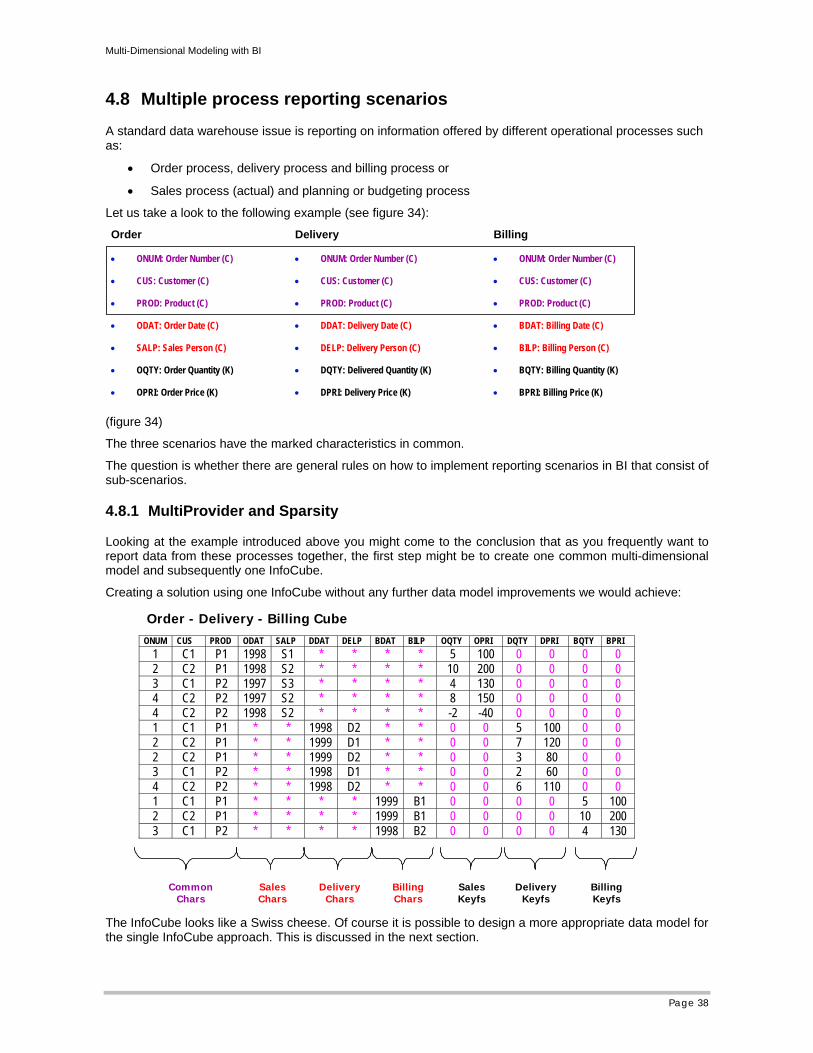
Multi-Dimensional Modeling with BI
Page 38
4.8 Multiple process reporting scenarios
A standard data warehouse issue is reporting on information offered by different operational processes such as:
• Order process, delivery process and billing process or
• Sales process (actual) and planning or budgeting process
Let us take a look to the following example (see figure 34):
Order
• ONUM: Order Number (C)
• CUS: Customer (C)
• PROD: Product (C)
• ODAT: Order Date (C)
• SALP: Sales Person (C)
• OQTY: Order Quantity (K)
• OPRI: Order Price (K)
Delivery
• ONUM: Order Number (C)
• CUS: Customer (C)
• PROD: Product (C)
• DDAT: Delivery Date (C)
• DELP: Delivery Person (C)
• DQTY: Delivered Quantity (K)
• DPRI: Delivery Price (K)
Billing
• ONUM: Order Number (C)
• CUS: Customer (C)
• PROD: Product (C)
• BDAT: Billing Date (C)
• BILP: Billing Person (C)
• BQTY: Billing Quantity (K)
• BPRI: Billing Price (K)
(figure 34)
The three scenarios have the marked characteristics in common.
The question is whether there are general rules on how to implement reporting scenarios in BI that consist of sub-scenarios.
4.8.1 MultiProvider and Sparsity
Looking at the example introduced above you might come to the conclusion that as you frequently want to report data from these processes together, the first step might be to create one common multi-dimensional model and subsequently one InfoCube.
Creating a solution using one InfoCube without any further data model improvements we would achieve:
ONUM CUS PROD ODAT SALP DDAT DELP BDAT BILP OQTY OPRI DQTY DPRI BQTY BPRI1 C1 P1 1998 S1 * * * * 5 100 0 0 0 02 C2 P1 1998 S2 * * * * 10 200 0 0 0 03 C1 P2 1997 S3 * * * * 4 130 0 0 0 04 C2 P2 1997 S2 * * * * 8 150 0 0 0 04 C2 P2 1998 S2 * * * * -2 -40 0 0 0 01 C1 P1 * * 1998 D2 * * 0 0 5 100 0 02 C2 P1 * * 1999 D1 * * 0 0 7 120 0 02 C2 P1 * * 1999 D2 * * 0 0 3 80 0 03 C1 P2 * * 1998 D1 * * 0 0 2 60 0 04 C2 P2 * * 1998 D2 * * 0 0 6 110 0 01 C1 P1 * * * * 1999 B1 0 0 0 0 5 1002 C2 P1 * * * * 1999 B1 0 0 0 0 10 2003 C1 P2 * * * * 1998 B2 0 0 0 0 4 130
Order - Delivery - Billing Cube
CommonChars
SalesChars
DeliveryChars
BillingChars
SalesKeyfs
DeliveryKeyfs
BillingKeyfs
The InfoCube looks like a Swiss cheese. Of course it is possible to design a more appropriate data model for the single InfoCube approach. This is discussed in the next section.

Multi-Dimensional Modeling with BI
Page 39
Using the BI MultiProvider functionality we can use a space-saving, better performing and more transparent approach. A MultiProvider is a a view on different InfoCubes which store the data. So, a MultiProvider is a virtual InfoCube that does not store the data physically. We define three standard InfoCubes, which serve as the input for the MultiProvider definition. The following has to be observed:
• Only characteristics and navigational attributes that reference the same InfoObject can be declared to be the same.
• If a characteristic of the MultiProvider is not contained in one of the standard InfoCubes, then the characteristic value with respect to this standard InfoCube is set initial.
• If the same InfoObject of type key figure occurs multiple times you have to decide whether to add the values from the different cubes or choose one key figure from one cube. In some scenarios the first option makes sense (for example: MultiProvider of country-specific basic cubes with revenue data) with other scenarios (example: actual and plan) this would be nonsensical.
• The best way to handle key figures is to use a key figure InfoObject not in different semantic constellations such as key figure QTY for ordered quantity in the order cube and for invoiced quantity in the invoiced cube as this allows you to access multiple InfoCubes within one query.
With this background we can create three Infocubes:
Order InfoCube
Delivery InfoCube
Billing InfoCube
Based on these InfoCubes a MultiProvider, a query showing sales and delivered quantity, would look like this:
Drilling down to salesperson will show the following results:
ONUM CUS PROD ODAT SALP OQTY OPRI 1 C1 P1 1998 S1 5 100 2 C2 P1 1998 S2 10 200 3 C1 P2 1997 S3 4 130 4 C2 P2 1997 S2 8 150 4 C2 P2 1998 S2 -2 -40
ONUM CUS PROD DDAT DELP DQTY DPRI 1 C1 P1 1998 D2 5 100 2 C2 P1 1999 D1 7 120 2 C2 P1 1999 D2 3 80 3 C1 P2 1998 D1 2 60 4 C2 P2 1998 D2 6 110
ONUM CUS PROD BDAT SALP BQTY BPRI 1 C1 P1 1999 B1 5 100 2 C2 P1 1999 B1 10 200 3 C1 P2 1998 B2 4 130
PROD SQTY DQTY P1 15 15 P2 10 8
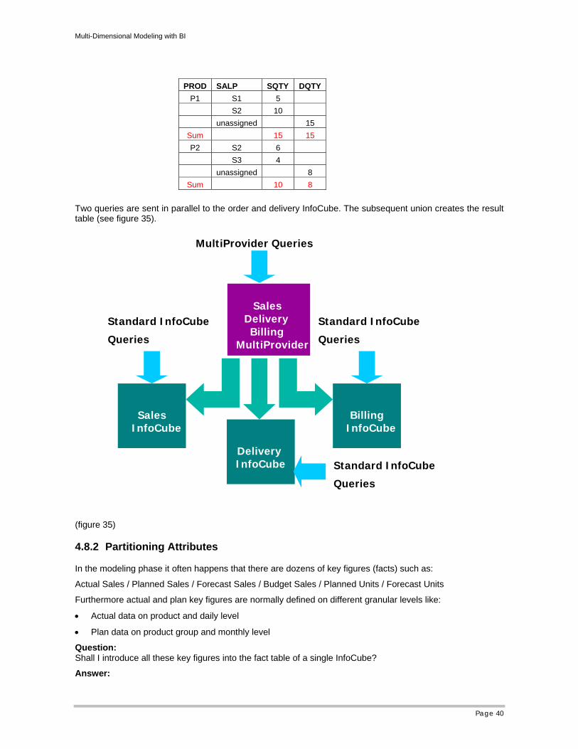
Multi-Dimensional Modeling with BI
Page 40
Two queries are sent in parallel to the order and delivery InfoCube. The subsequent union creates the result table (see figure 35).
(figure 35)
4.8.2 Partitioning Attributes
In the modeling phase it often happens that there are dozens of key figures (facts) such as:
Actual Sales / Planned Sales / Forecast Sales / Budget Sales / Planned Units / Forecast Units
Furthermore actual and plan key figures are normally defined on different granular levels like:
• Actual data on product and daily level
• Plan data on product group and monthly level
Question: Shall I introduce all these key figures into the fact table of a single InfoCube?
Answer:
PROD SALP SQTY DQTY P1 S1 5
S2 10 unassigned 15
Sum 15 15 P2 S2 6
S3 4 unassigned 8
Sum 10 8
Sales InfoCube
BillingInfoCube
SalesDeliveryBilling
MultiProvider
MultiProvider Queries
Standard InfoCube
Queries
Standard InfoCube
Queries
Delivery InfoCube Standard InfoCube
Queries
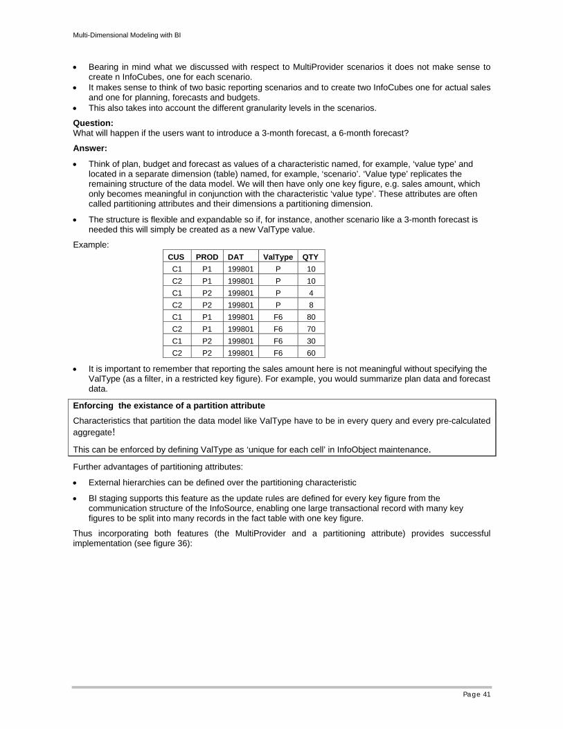
Multi-Dimensional Modeling with BI
Page 41
• Bearing in mind what we discussed with respect to MultiProvider scenarios it does not make sense to create n InfoCubes, one for each scenario.
• It makes sense to think of two basic reporting scenarios and to create two InfoCubes one for actual sales and one for planning, forecasts and budgets.
• This also takes into account the different granularity levels in the scenarios.
Question: What will happen if the users want to introduce a 3-month forecast, a 6-month forecast?
Answer:
• Think of plan, budget and forecast as values of a characteristic named, for example, ‘value type’ and located in a separate dimension (table) named, for example, ‘scenario’. ‘Value type’ replicates the remaining structure of the data model. We will then have only one key figure, e.g. sales amount, which only becomes meaningful in conjunction with the characteristic ‘value type’. These attributes are often called partitioning attributes and their dimensions a partitioning dimension.
• The structure is flexible and expandable so if, for instance, another scenario like a 3-month forecast is needed this will simply be created as a new ValType value.
Example: CUS PROD DAT ValType QTY
C1 P1 199801 P 10 C2 P1 199801 P 10 C1 P2 199801 P 4 C2 P2 199801 P 8 C1 P1 199801 F6 80 C2 P1 199801 F6 70 C1 P2 199801 F6 30 C2 P2 199801 F6 60
• It is important to remember that reporting the sales amount here is not meaningful without specifying the ValType (as a filter, in a restricted key figure). For example, you would summarize plan data and forecast data.
Enforcing the existance of a partition attribute
Characteristics that partition the data model like ValType have to be in every query and every pre-calculated aggregate!
This can be enforced by defining ValType as ‘unique for each cell’ in InfoObject maintenance.
Further advantages of partitioning attributes:
• External hierarchies can be defined over the partitioning characteristic
• BI staging supports this feature as the update rules are defined for every key figure from the communication structure of the InfoSource, enabling one large transactional record with many key figures to be split into many records in the fact table with one key figure.
Thus incorporating both features (the MultiProvider and a partitioning attribute) provides successful implementation (see figure 36):
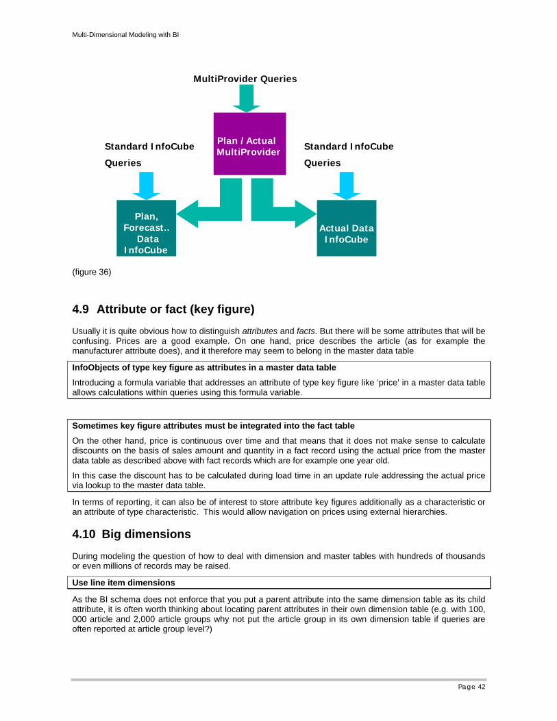
Multi-Dimensional Modeling with BI
Page 42
(figure 36)
4.9 Attribute or fact (key figure)
Usually it is quite obvious how to distinguish attributes and facts. But there will be some attributes that will be confusing. Prices are a good example. On one hand, price describes the article (as for example the manufacturer attribute does), and it therefore may seem to belong in the master data table
InfoObjects of type key figure as attributes in a master data table
Introducing a formula variable that addresses an attribute of type key figure like ‘price’ in a master data table allows calculations within queries using this formula variable.
Sometimes key figure attributes must be integrated into the fact table
On the other hand, price is continuous over time and that means that it does not make sense to calculate discounts on the basis of sales amount and quantity in a fact record using the actual price from the master data table as described above with fact records which are for example one year old.
In this case the discount has to be calculated during load time in an update rule addressing the actual price via lookup to the master data table.
In terms of reporting, it can also be of interest to store attribute key figures additionally as a characteristic or an attribute of type characteristic. This would allow navigation on prices using external hierarchies.
4.10 Big dimensions
During modeling the question of how to deal with dimension and master tables with hundreds of thousands or even millions of records may be raised.
Use line item dimensions
As the BI schema does not enforce that you put a parent attribute into the same dimension table as its child attribute, it is often worth thinking about locating parent attributes in their own dimension table (e.g. with 100, 000 article and 2,000 article groups why not put the article group in its own dimension table if queries are often reported at article group level?)
Plan, Forecast..
Data InfoCube
Actual DataInfoCube
Plan /ActualMultiProvider
MultiProvider Queries
Standard InfoCube
Queries
Standard InfoCube
Queries
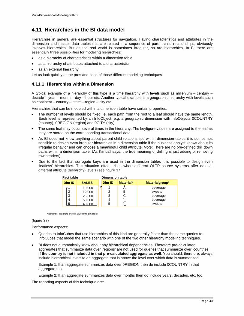
Multi-Dimensional Modeling with BI
Page 43
4.11 Hierarchies in the BI data model
Hierarchies in general are essential structures for navigation. Having characteristics and attributes in the dimension and master data tables that are related in a sequence of parent-child relationships, obviously involves hierarchies. But as the real world is sometimes irregular, so are hierarchies. In BI there are essentially three possibilities for modeling hierarchies: • as a hierarchy of characteristics within a dimension table • as a hierarchy of attributes attached to a characteristic • as an external hierarchy Let us look quickly at the pros and cons of those different modeling techniques.
4.11.1 Hierarchies within a Dimension
A typical example of a hierarchy of this type is a time hierarchy with levels such as millenium – century – decade – year – month – day – hour etc. Another typical example is a geographic hierarchy with levels such as continent – country – state – region – city etc.
Hierarchies that can be modeled within a dimension table have certain properties: • The number of levels should be fixed i.e. each path from the root to a leaf should have the same length.
Each level is represented by an InfoObject, e.g. a geographic dimension with InfoObjects 0COUNTRY (country), 0REGION (region) and 0CITY (city).
• The same leaf may occur several times in the hierarchy. The keyfigure values are assigned to the leaf as they are stored on the corresponding transactional data.
• As BI does not know anything about parent-child relationships within dimension tables it is sometimes sensible to design even irregular hierarchies in a dimension table if the business analyst knows about its irregular behavior and can choose a meaningful child attribute. Note: There are no pre-defined drill down paths within a dimension table. (As Kimball says, the true meaning of drilling is just adding or removing row headers).
• Due to the fact that surrogate keys are used in the dimension tables it is possible to design even ‘leafless’ hierarchies. This situation often arises when different OLTP source systems offer data at different attribute (hierarchy) levels (see figure 37):
ABC'_''_'
Dim ID Umsatz Dim ID Material* Materialgroup*12345
10.00012.00025.00050.00040.000
Fact table Dimension tableDim ID SALES
beveragesweetsbeveragebeveragesweets
* remember that there are only SIDs in the dim table !
12345
(figure 37)
Performance aspects:
• Queries to InfoCubes that use hierarchies of this kind are generally faster than the same queries to InfoCubes that model the same scenario with one of the two other hierarchy modeling techniques.
• BI does not automatically know about any hierarchical dependencies. Therefore pre-calculated aggregates that summarize data over ‘regions’ are not used for queries that summarize over ‘countries’ if the country is not included in that pre-calculated aggregate as well. You should, therefore, always include hierarchical levels to an aggregate that is above the level over which data is summarized.
Example 1: If an aggregate summarizes data over 0REGION then do include 0COUNTRY in that aggregate too.
Example 2: If an aggregate summarizes data over months then do include years, decades, etc. too.
The reporting aspects of this technique are:
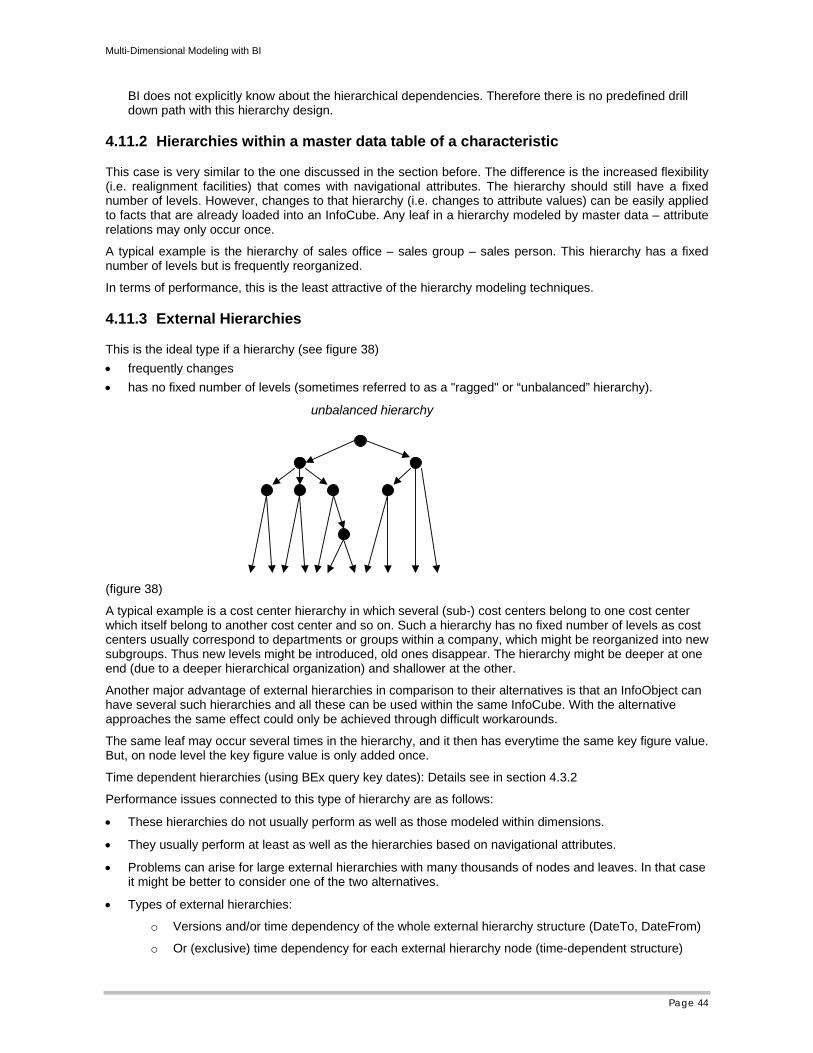
Multi-Dimensional Modeling with BI
Page 44
BI does not explicitly know about the hierarchical dependencies. Therefore there is no predefined drill down path with this hierarchy design.
4.11.2 Hierarchies within a master data table of a characteristic
This case is very similar to the one discussed in the section before. The difference is the increased flexibility (i.e. realignment facilities) that comes with navigational attributes. The hierarchy should still have a fixed number of levels. However, changes to that hierarchy (i.e. changes to attribute values) can be easily applied to facts that are already loaded into an InfoCube. Any leaf in a hierarchy modeled by master data – attribute relations may only occur once.
A typical example is the hierarchy of sales office – sales group – sales person. This hierarchy has a fixed number of levels but is frequently reorganized.
In terms of performance, this is the least attractive of the hierarchy modeling techniques.
4.11.3 External Hierarchies
This is the ideal type if a hierarchy (see figure 38) • frequently changes • has no fixed number of levels (sometimes referred to as a "ragged" or “unbalanced” hierarchy).
unbalanced hierarchy
(figure 38)
A typical example is a cost center hierarchy in which several (sub-) cost centers belong to one cost center which itself belong to another cost center and so on. Such a hierarchy has no fixed number of levels as cost centers usually correspond to departments or groups within a company, which might be reorganized into new subgroups. Thus new levels might be introduced, old ones disappear. The hierarchy might be deeper at one end (due to a deeper hierarchical organization) and shallower at the other.
Another major advantage of external hierarchies in comparison to their alternatives is that an InfoObject can have several such hierarchies and all these can be used within the same InfoCube. With the alternative approaches the same effect could only be achieved through difficult workarounds.
The same leaf may occur several times in the hierarchy, and it then has everytime the same key figure value. But, on node level the key figure value is only added once.
Time dependent hierarchies (using BEx query key dates): Details see in section 4.3.2
Performance issues connected to this type of hierarchy are as follows:
• These hierarchies do not usually perform as well as those modeled within dimensions.
• They usually perform at least as well as the hierarchies based on navigational attributes.
• Problems can arise for large external hierarchies with many thousands of nodes and leaves. In that case it might be better to consider one of the two alternatives.
• Types of external hierarchies:
o Versions and/or time dependency of the whole external hierarchy structure (DateTo, DateFrom)
o Or (exclusive) time dependency for each external hierarchy node (time-dependent structure)