Embed Size (px)
Citation preview

Moving Towards Deep Learning Algorithms on HPCC Systems
Maryam M. Najafabadi
Overview
• L-BFGS
• HPCC Systems
• Implementation of L-BFGS on HPCC Systems
• SoftMax
• Sparse Autoencoder
• Toward Deep Learning
2

Mathematical optimization
• Minimizing/Maximizing a function
Minimum
3
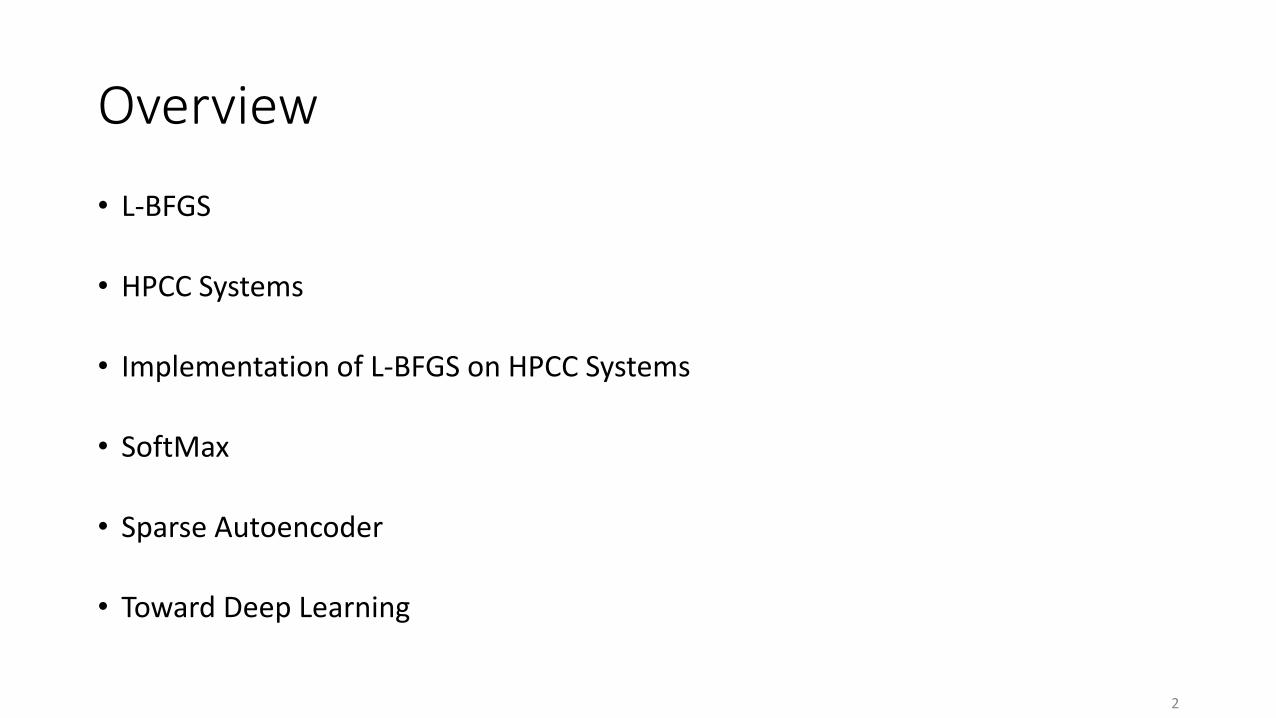
Optimization Algorithms in Machine Learning
• Linear Regression
Minimize Errors
4
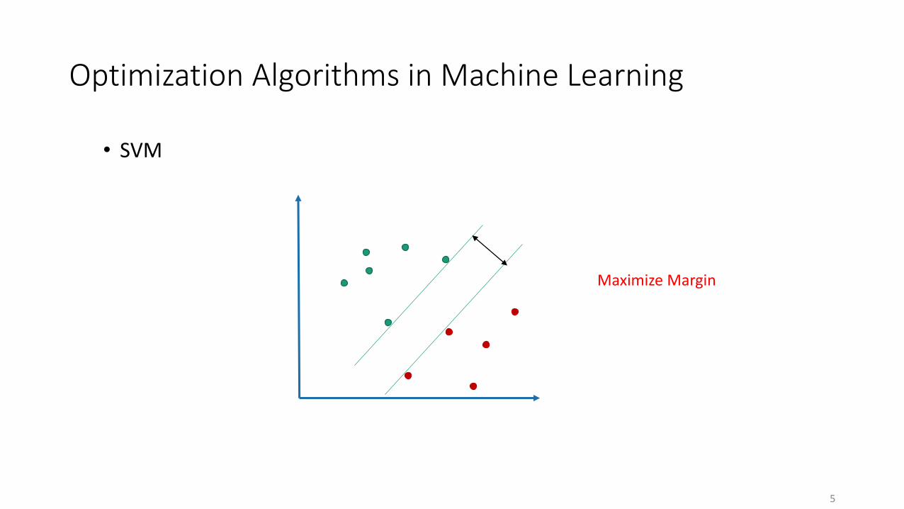
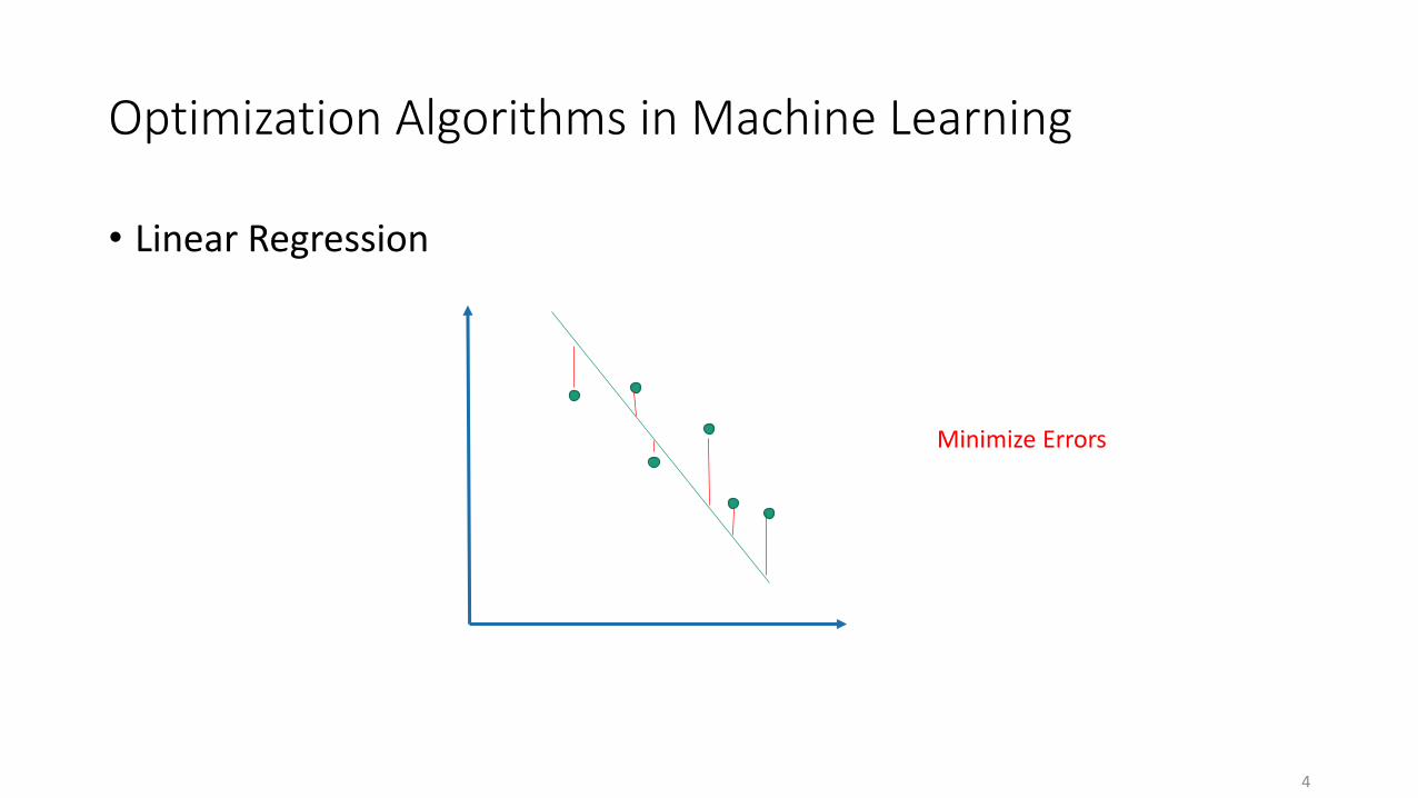
Optimization Algorithms in Machine Learning
• SVM
Maximize Margin
5
Optimization Algorithms in Machine Learning
• Collaborative filtering
• K-means
• Maximum likelihood estimation
• Graphical models
• Neural Networks
• Deep Learning
6

Formulate Training as an Optimization Problem
• Training model: finding parameters that minimize some objective function
Define ParametersDefine an Objective
FunctionFind values for the parameters that
minimize the objective function
Cost term Regularization term
Optimization Algorithm
7
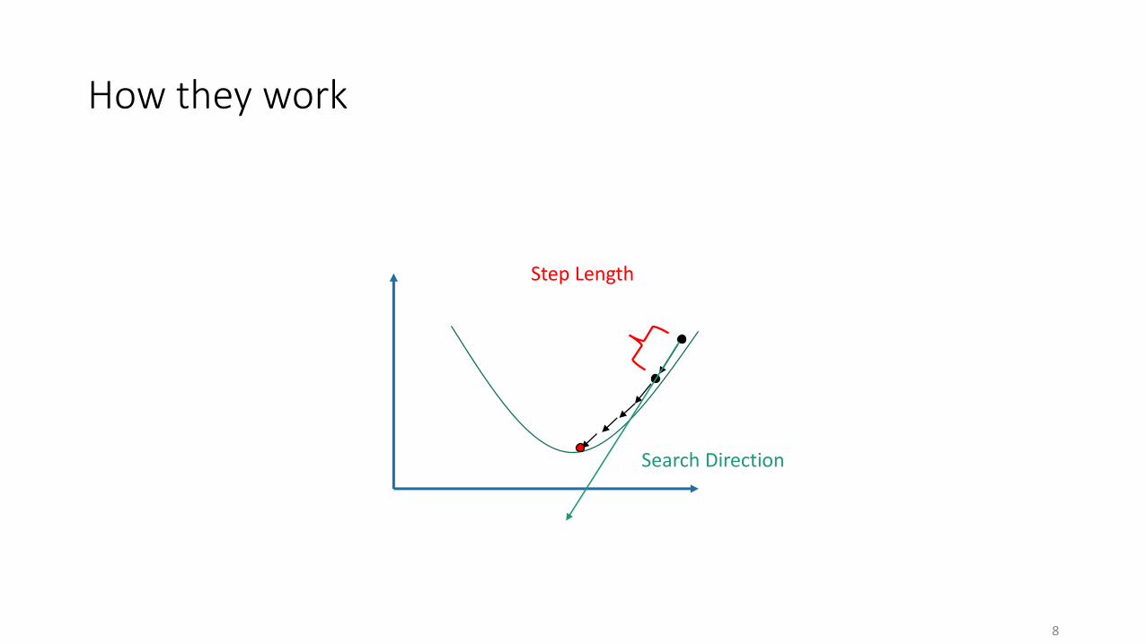
How they work
Search Direction
Step Length
8

Gradient Descent
• Step length• Constant value
• Search direction• Negative gradient
9

Gradient Descent
• Step length• Constant value
• Search direction• Negative gradient
Small Step Length
10
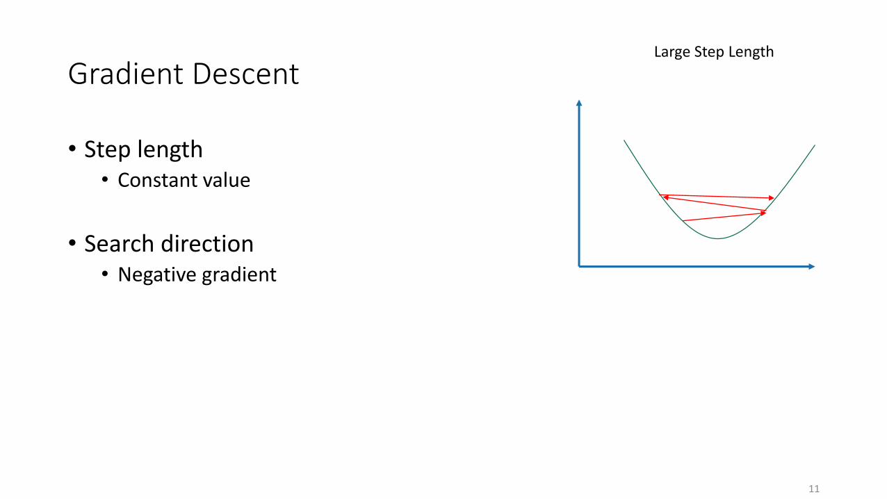
Gradient Descent
• Step length• Constant value
• Search direction• Negative gradient
Large Step Length
11

Newton Methods
• Step length• Use a line search
• Search direction• Use Curative Information (Inverse of Hessian Matrix)
12
Quasi Newton Methods
• Problem with large n in Newton methods• Calculation of inverse of Hessian matrix too expensive
• Continuously updating an approximation of the inverse of the Hessian matrix in each iteration
13

BFGS
• Broyden, Fletcher, Goldfarb, and Shanno
• Most popular Quasi Newton Method
• Uses Wolfe line search to find step length
• Needs to keep n×n matrix in memory
14

L-BFGS
• Limited-memory: only a few vectors of length n (m×n instead of n×n)
• m << n
• Useful for solving large problems (large n)
• More stable learning
• Uses curvature information to take a more direct route • faster convergence
15

How to use
• Define a function that calculates Objective value and Gradient
ObjectiveFunc (x, ObjectiveFunc_params, TrainData , TrainLabel)
16
Why L-BFGS?
• Toward Deep Learning• Optimization is heart of DL and many other ML algorithms
• Popular
• Advantages over SGD
17

HPCC Systems
• Open source, massive parallel-processing computing platform for big data processing and analytics
• LexisNexis Risk Solutions
• Uses commodity clusters of hardware running on top of the Linux operating system
• Based on DataFlow programming model
• THOR-ROXIE
• ECL
18
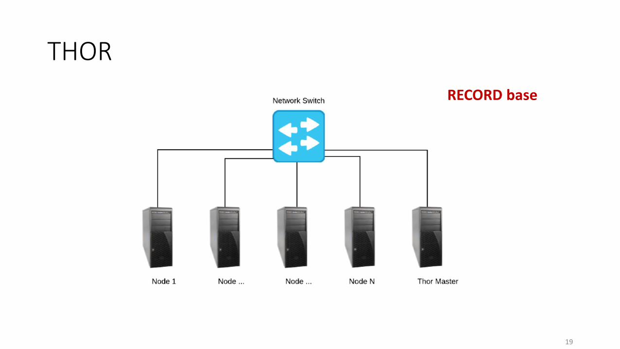
THOR
19
RECORD base

DataFlow Analysis
• Main focus is how the data is being changed
• A Graph represents a transformation on the data
• Each node is an operation
• Edges show the data flow
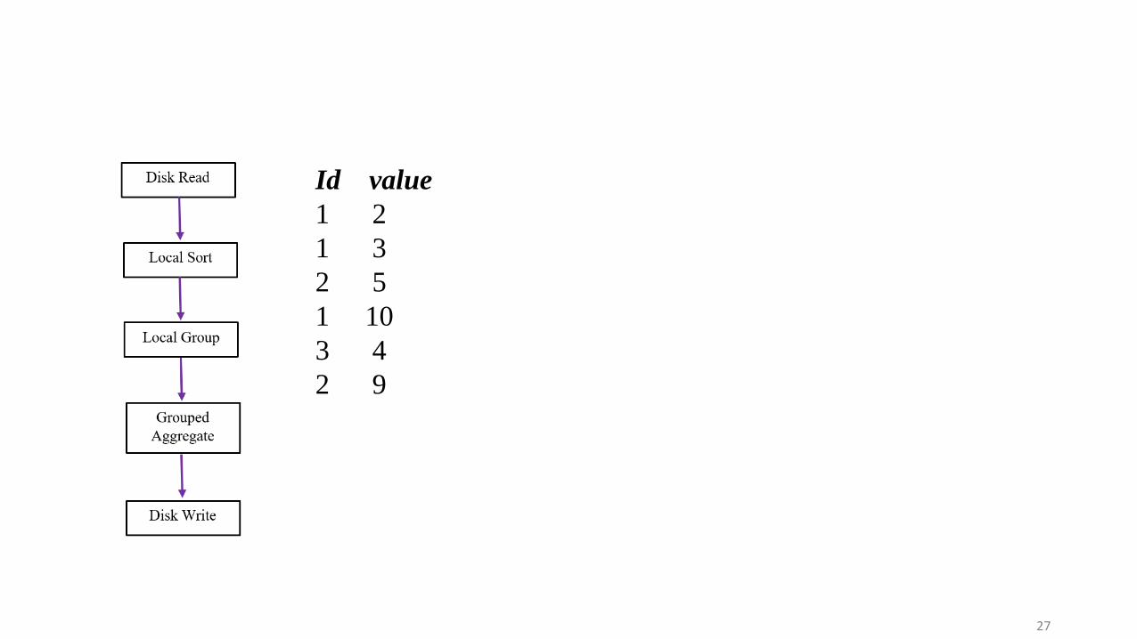
20

A DataFlow example
21
Id value
1 2
1 3
2 5
1 10
3 4
2 9
Id value
1 2
1 3
1 10
2 5
2 9
3 4
Id value
1 10
2 9
3 4
MAX

ECL
• Enterprise Control Language
• Compiled into optimized C++ code
• Declarative Language provides parallel and distributed DataFloworiented processing
22

ECL
• Enterprise Control Language
• Compiled into optimized C++ code
• Declarative Language provides parallel and distributed DataFloworiented processing
23
Declarative
• What to accomplish, rather than How to accomplish
• You’re describing what you’re trying to achieve, without instructing how to do it
24
ECL
• Enterprise Control Language
• Compiled into optimized C++ code
• Declarative Language provides parallel and distributed DataFloworiented processing
25

ECL
• Enterprise Control Language
• Compiled into optimized C++ code
• Declarative Language provides parallel and distributed DataFloworiented processing
26
27
Id value
1 2
1 3
2 5
1 10
3 4
2 9
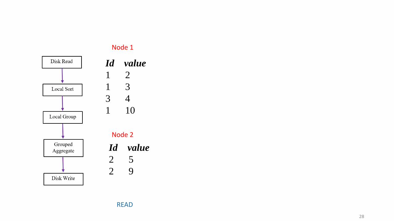
28
Id value
2 5
2 9
Node 1
Node 2
READ
Id value
1 2
1 3
3 4
1 10
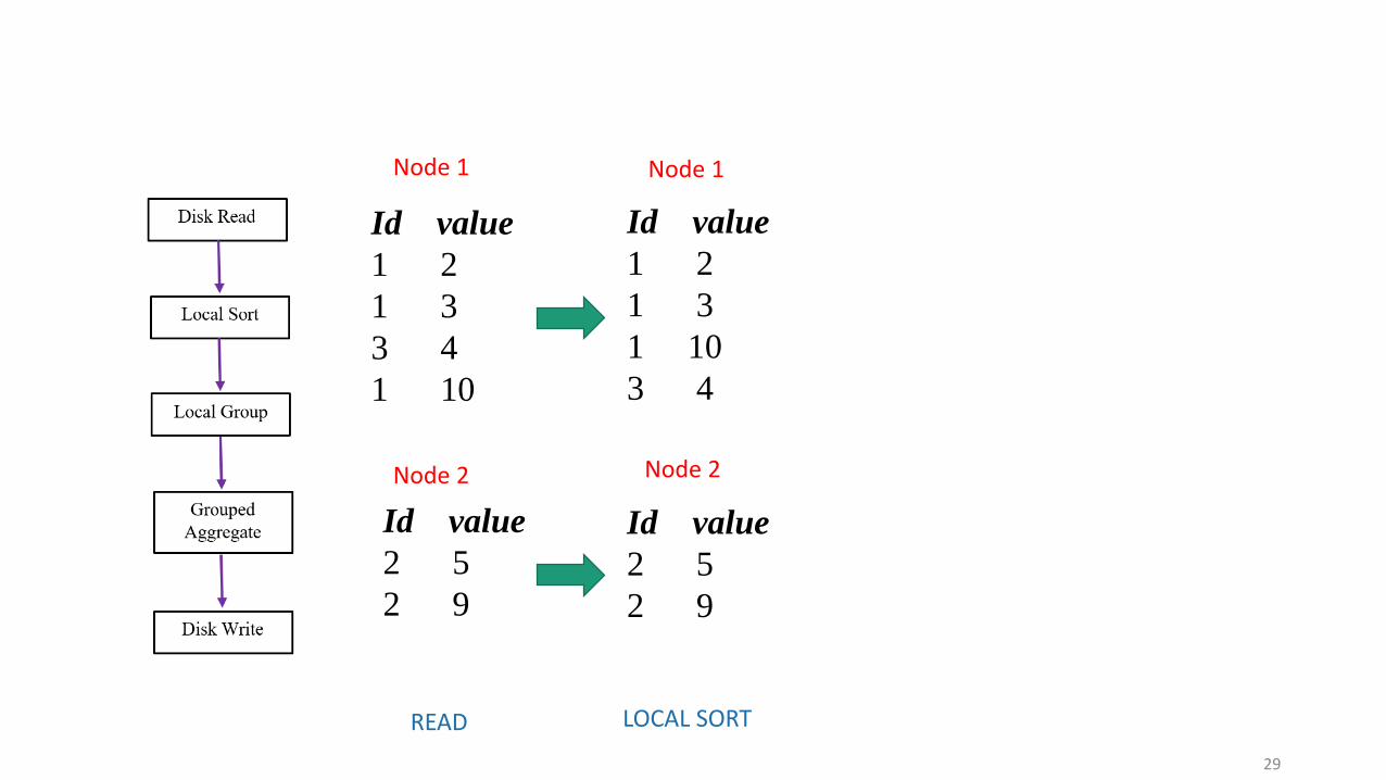
29
Id value
2 5
2 9
Node 1
Node 2
LOCAL SORT
Id value
1 2
1 3
1 10
3 4
Id value
2 5
2 9
Node 1
Node 2
READ
Id value
1 2
1 3
3 4
1 10
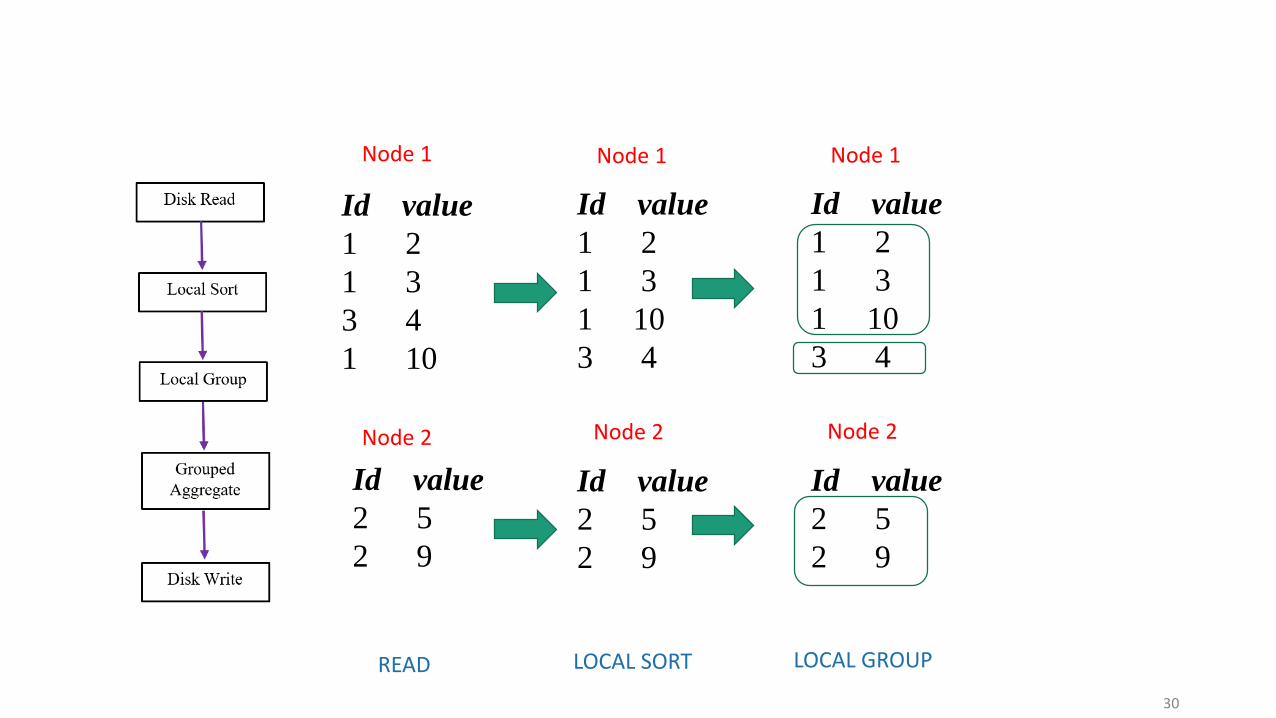
30
Id value
2 5
2 9
Node 1
Node 2
LOCAL SORT
Id value
1 2
1 3
1 10
3 4
Id value
2 5
2 9
Node 1
Node 2
READ
Id value
1 2
1 3
3 4
1 10
Id value
1 2
1 3
1 10
3 4
Id value
2 5
2 9
Node 1
Node 2
LOCAL GROUP

31
Id value
2 5
2 9
Node 1
Node 2
LOCAL SORT
Id value
1 2
1 3
1 10
3 4
Id value
2 5
2 9
Node 1
Node 2
READ
Id value
1 2
1 3
3 4
1 10
Id value
1 2
1 3
1 10
3 4
Id value
2 5
2 9
Node 1
Node 2
LOCAL GROUP
Id value
1 10
3 4
Id value
2 9
Node 1
Node 2
LOCAL AGG/MAX

Back to L-BFGS
• Minimize f(x)
• Start with an initialized x : x0
• Repeatedly update: xk+1 = xk + αkpk
32
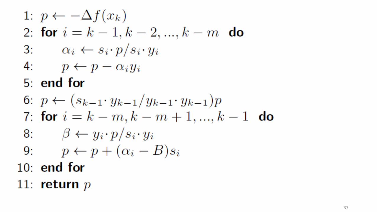
Wolfe line search L-BFGS

• If x too large it does not fit in memory of one machine
• Needs m × n memory
• Distribute x on different machines
• Try to do computations locally
• Do global computations as necessary
33
• If x too large it does not fit in memory of one machine
• Needs m × n memory
• Distribute x on different machines
• Try to do computations locally
• Do global computations as necessary
34

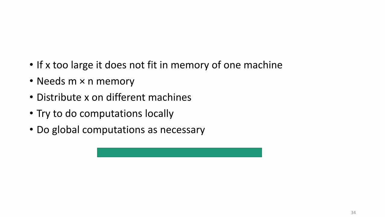
• If x too large it does not fit in memory of one machine
• Needs m × n memory
• Distribute x on different machines
• Try to do computations locally
• Do global computations as necessary
35
. . .

• If x too large it does not fit in memory of one machine
• Needs m × n memory
• Distribute x on different machines
• Try to do computations locally
• Do global computations as necessary
36
. . .
. . .
37
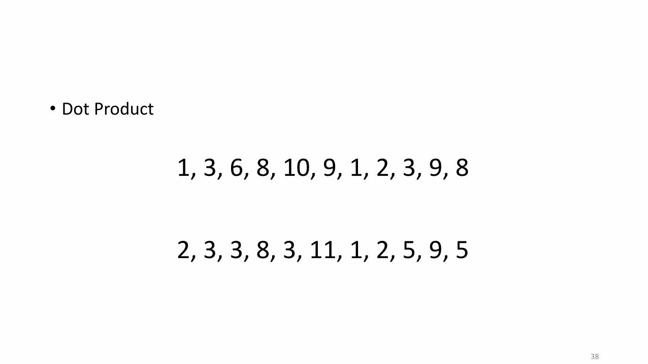
• Dot Product
38
1, 3, 6, 8, 10, 9, 1, 2, 3, 9, 8
2, 3, 3, 8, 3, 11, 1, 2, 5, 9, 5

• Dot Product
39
1, 3, 6, 8
3, 11, 1, 2
10, 9, 1, 2 3, 9, 8
Node 1 Node 2 Node 3
5, 9, 5 2, 3, 3, 8
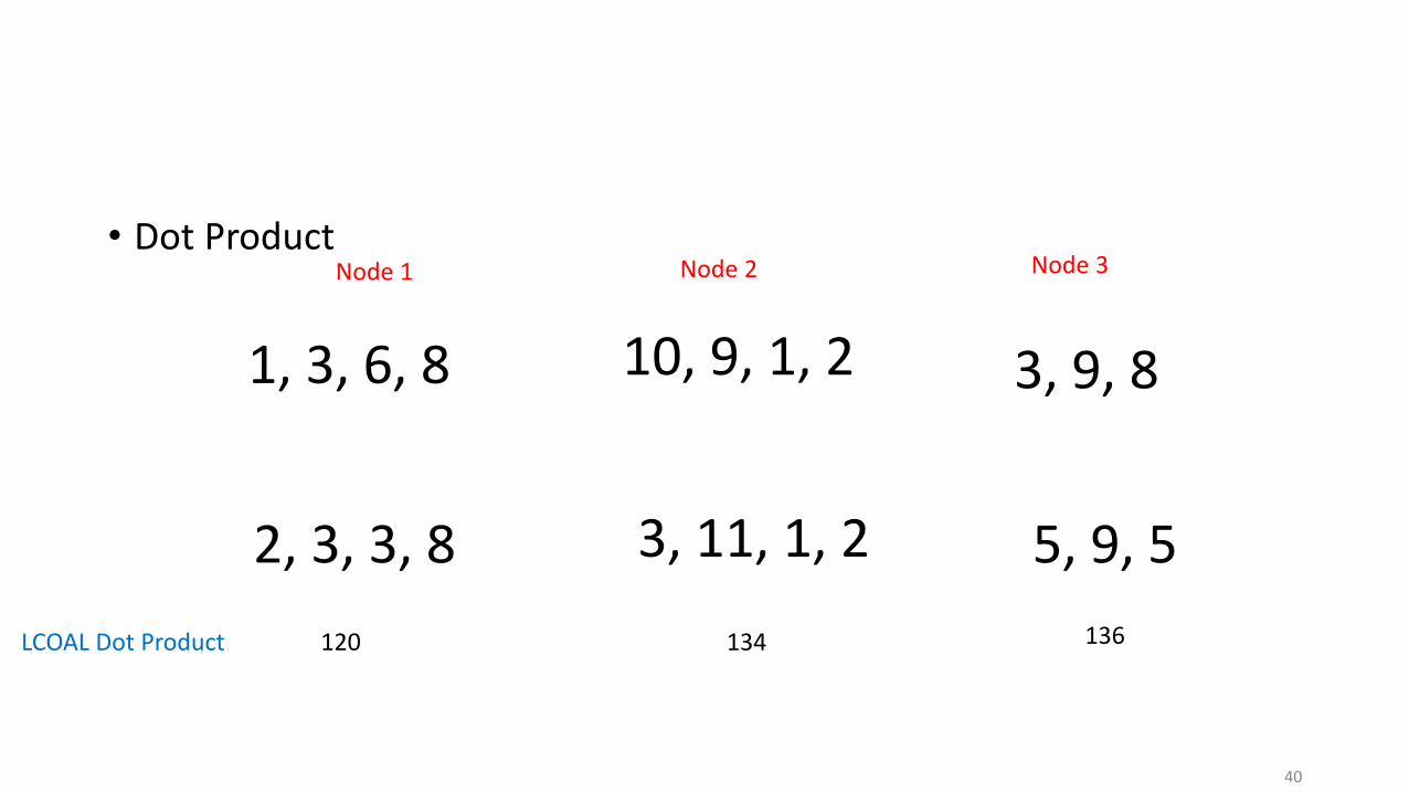
• Dot Product
40
1, 3, 6, 8
3, 11, 1, 2
10, 9, 1, 2 3, 9, 8
Node 1 Node 2 Node 3
5, 9, 5 2, 3, 3, 8
LCOAL Dot Product 120 134 136
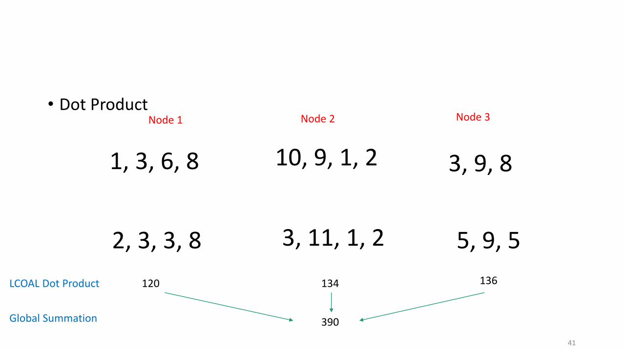
• Dot Product
41
1, 3, 6, 8
3, 11, 1, 2
10, 9, 1, 2 3, 9, 8
Node 1 Node 2 Node 3
5, 9, 5 2, 3, 3, 8
LCOAL Dot Product
Global Summation
120 134 136
390

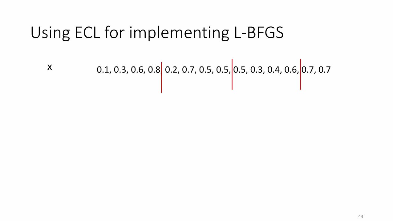
Using ECL for implementing L-BFGS
42
0.1, 0.3, 0.6, 0.8, 0.2, 0.7, 0.5, 0.5, 0.5, 0.3, 0.4, 0.6, 0.7, 0.7x
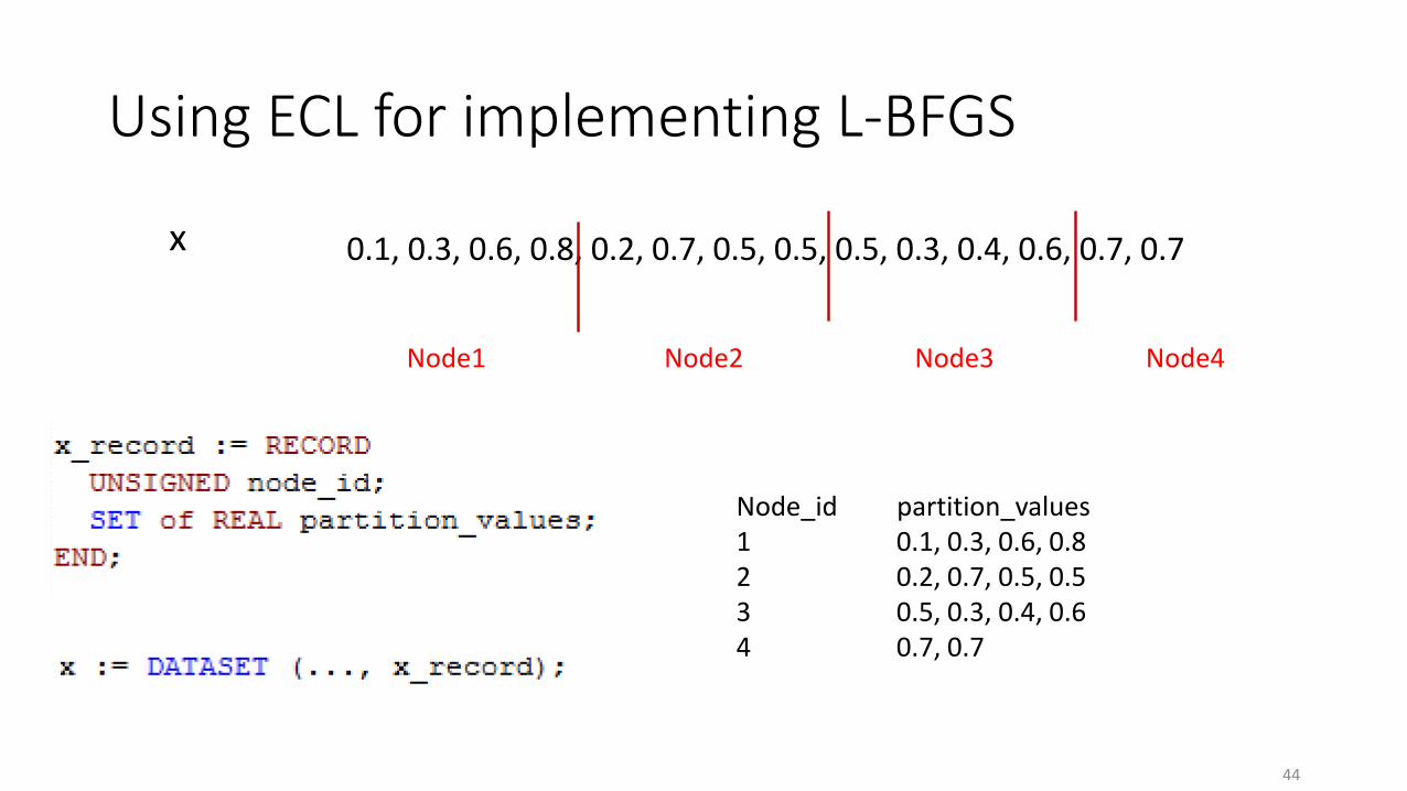
Using ECL for implementing L-BFGS
43
0.1, 0.3, 0.6, 0.8, 0.2, 0.7, 0.5, 0.5, 0.5, 0.3, 0.4, 0.6, 0.7, 0.7x
Using ECL for implementing L-BFGS
44
0.1, 0.3, 0.6, 0.8, 0.2, 0.7, 0.5, 0.5, 0.5, 0.3, 0.4, 0.6, 0.7, 0.7x
Node1 Node2 Node3 Node4
Node_id partition_values1 0.1, 0.3, 0.6, 0.82 0.2, 0.7, 0.5, 0.53 0.5, 0.3, 0.4, 0.64 0.7, 0.7

Using ECL for implementing L-BFGS
45
0.1, 0.3, 0.6, 0.8, 0.2, 0.7, 0.5, 0.5, 0.5, 0.3, 0.4, 0.6, 0.7, 0.7x
Node1 Node2 Node3 Node4
Node_id partition_values1 0.1, 0.3, 0.6, 0.82 0.2, 0.7, 0.5, 0.53 0.5, 0.3, 0.4, 0.64 0.7, 0.7
Node 1
Node 4
Node 2
Node 3

Using ECL for implementing L-BFGS
46
0.1, 0.3, 0.6, 0.8, 0.2, 0.7, 0.5, 0.5, 0.5, 0.3, 0.4, 0.6, 0.7, 0.7x
Node_id partition_values1 0.1, 0.3, 0.6, 0.82 0.2, 0.7, 0.5, 0.53 0.5, 0.3, 0.4, 0.64 0.7, 0.7
Node 1
Node 4
Node 2
Node 3

Example of LOCAL operations
• Scale
47

Example of LOCAL operations
• Scale
48
Node_id partition_values1 0.1, 0.3, 0.6, 0.82 0.2, 0.7, 0.5, 0.53 0.5, 0.3, 0.4, 0.64 0.7, 0.7
Node 1
Node 4
Node 2
Node 3
x

Example of LOCAL operations
• Scale
49
Node_id partition_values1 1, 3, 682 2, 7, 5, 53 5, 3, 4, 64 7, 7
Node 1
Node 4
Node 2
Node 3
x_10
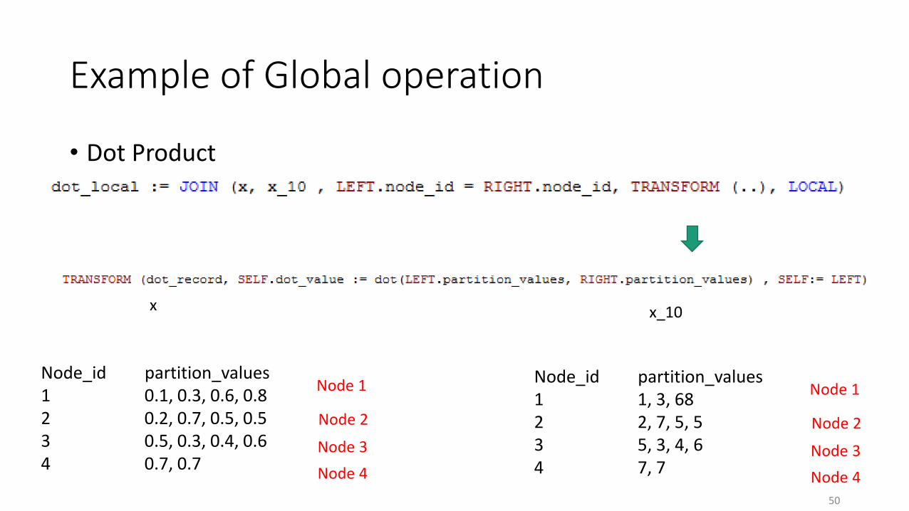
Example of Global operation
• Dot Product
50
Node_id partition_values1 0.1, 0.3, 0.6, 0.82 0.2, 0.7, 0.5, 0.53 0.5, 0.3, 0.4, 0.64 0.7, 0.7
Node 1
Node 4
Node 2
Node 3
Node_id partition_values1 1, 3, 682 2, 7, 5, 53 5, 3, 4, 64 7, 7
Node 1
Node 4
Node 2
Node 3
x x_10

Example of Global operation
• Dot Product
51
Node_id partition_values1 0.1, 0.3, 0.6, 0.82 0.2, 0.7, 0.5, 0.53 0.5, 0.3, 0.4, 0.64 0.7, 0.7
Node 1
Node 4
Node 2
Node 3
Node_id partition_values1 1, 3, 6, 82 2, 7, 5, 53 5, 3, 4, 64 7, 7
Node 1
Node 4
Node 2
Node 3
x x_10
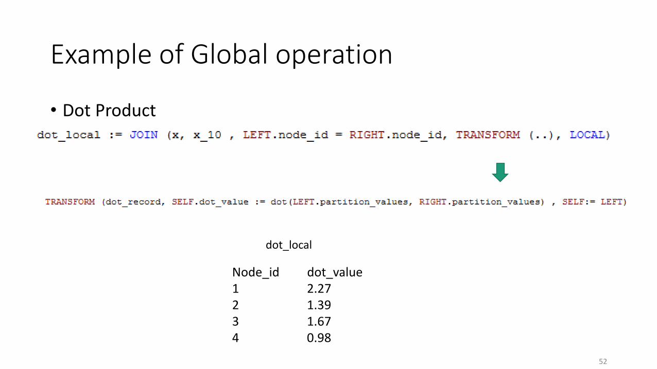
Example of Global operation
• Dot Product
52
Node_id dot_value1 2.272 1.393 1.674 0.98
dot_local
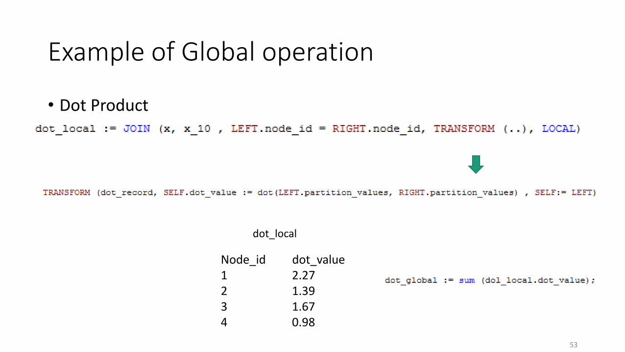
Example of Global operation
• Dot Product
53
Node_id dot_value1 2.272 1.393 1.674 0.98
dot_local
L-BFGS based Implementations
• Softmax
• Sparse Autoencoder
54

SoftMax Regression
• Generalizes logistic regression
• More than two classes
• MNIST -> 10 different classes
55

Formulate to an optimization problem
• Parameters• K × f variables
• Objective function• Generalize logistic regression objective function
• Define a function to calculate objective value and Gradient at a give point
56
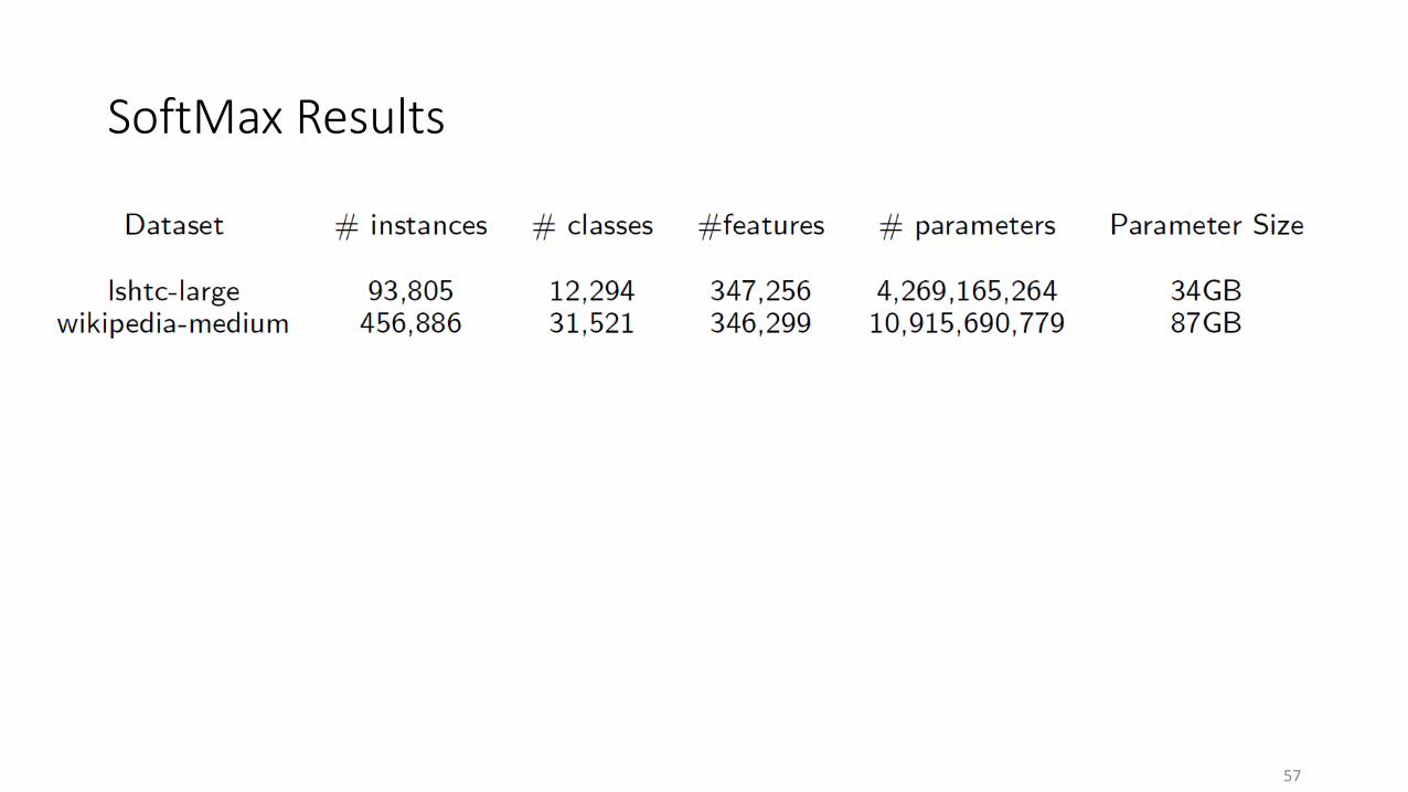
SoftMax Results
57

SoftMax Results
• Lshtc-large• 410 GB• 61 itr, 81 fun• 1 hour
• Wikipedia-medium• 1,048 GB• 12 itr, 21 fun• Half an hour
58
400 Nodes

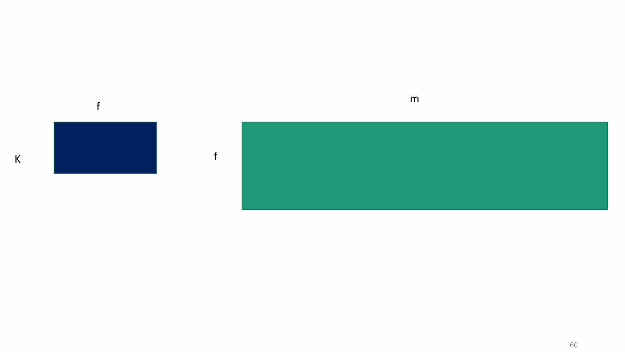
More Examples
• Parameter matrix in SoftMax: K × f
• Data Matrix: f × m
• Multiply these two matrix
• Result is K × m
59
60
K
f
f
m

If parameter matrix is small
61
K
f
f
m
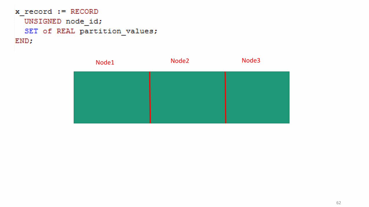
62
Node1 Node2 Node3

63
Node1 Node2 Node3
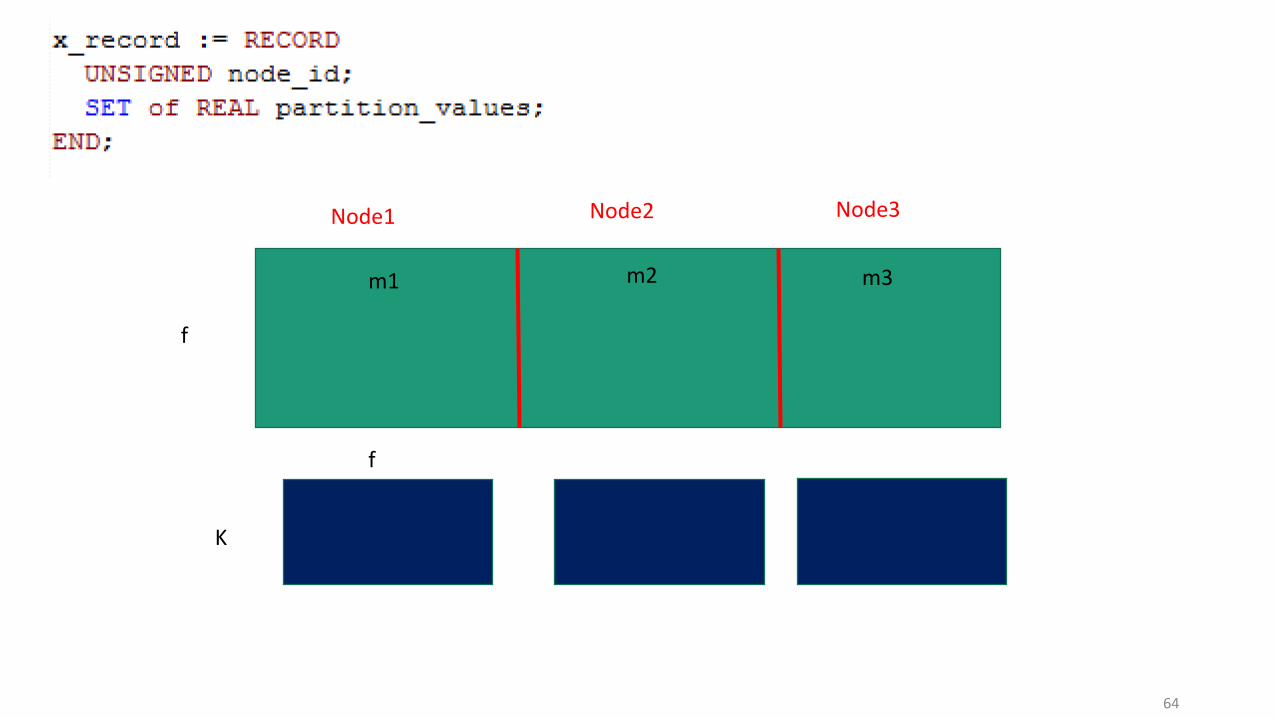
64
Node1 Node2 Node3
K
f
f
m1 m2 m3
65
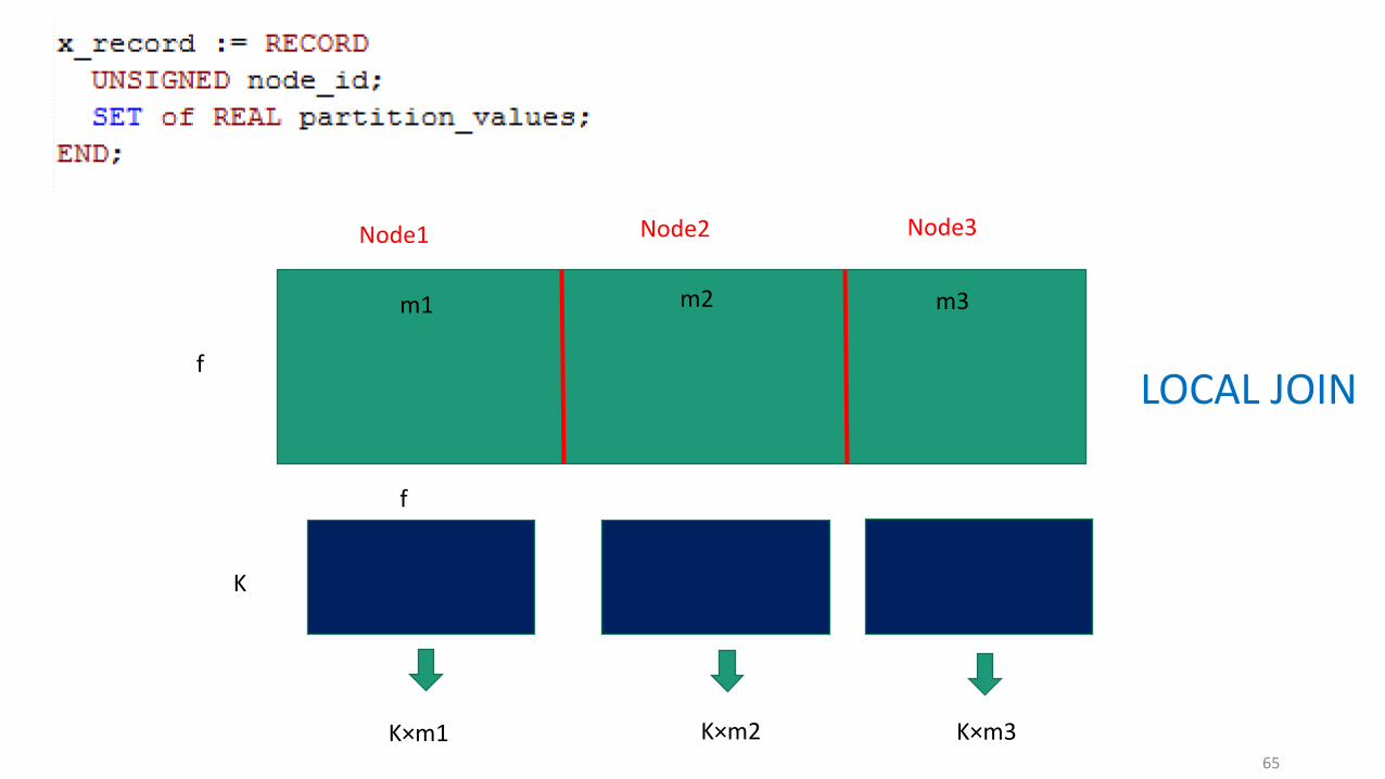
Node1 Node2 Node3
K
f
f
m1 m2 m3
LOCAL JOIN
K×m1 K×m2 K×m3
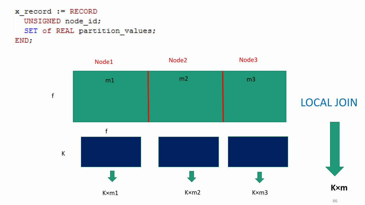
66
Node1 Node2 Node3
K
f
f
m1 m2 m3
LOCAL JOIN
K×m1 K×m2 K×m3K×m

If both matrices big
67
K
f
f
m

If both matrices big
68
f1
f
m2
K
m1m3
f2 f3

If both matrices big
69
f1
f
m
K
f2 f3
f1
f2
f3
K×m

If both matrices big
70
f1
f
m
K
f2 f3
f1
f2
f3
K×m K×m
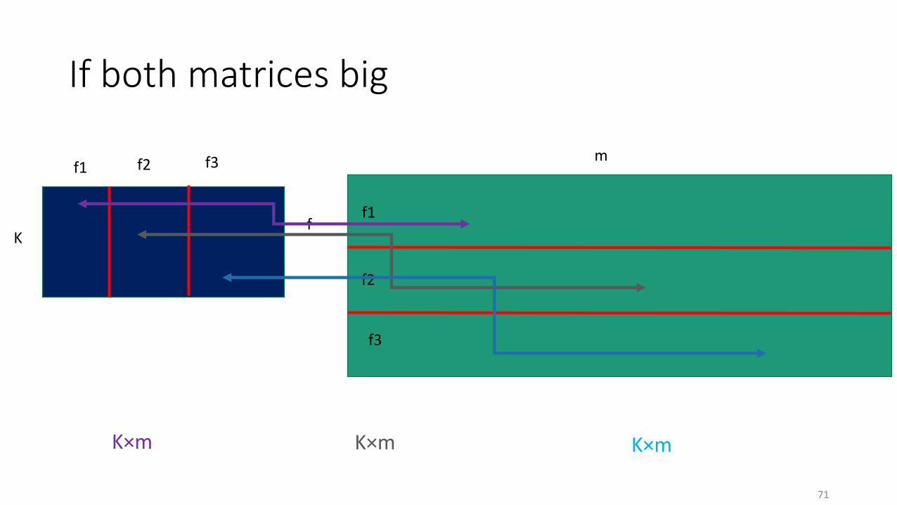
If both matrices big
71
f1
f
m
K
f2 f3
f1
f2
f3
K×m K×m K×m

If both matrices big
72
f1
f
m
K
f2 f3
f1
f2
f3
K×m K×m K×m ROLLUP
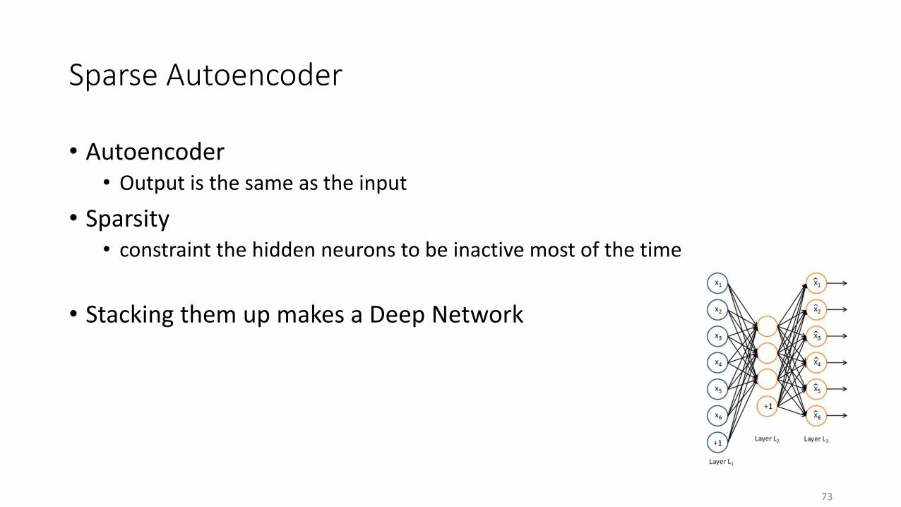
Sparse Autoencoder
• Autoencoder• Output is the same as the input
• Sparsity• constraint the hidden neurons to be inactive most of the time
• Stacking them up makes a Deep Network
73

Formulate to an optimization problem
• Parameters• Weight and bias values
• Objective function• Difference between output and expected output
• Penalty term to impose sparsity
• Define a function to calculate objective value and Gradient at a give point
74

Sparse Autoencoder results
• 10,000 samples of randomly 8×8 selected patches
75

Sparse Autoencoder results
• MNIST dataset
76
Toward Deep Learning
• Provide learned features from one layer to another sparse autoencoder
• …. Stack up to build a deep network
• Fine tuning • Using forward propagation to calculate cost value and back propagation to
calculate gradients
• Use L-BFGS to fine tune
77
SUMMARY
• HPCC Systems allows implementation of Large-scale ML algorithms
• Optimization Algorithms an important aspect for advanced machine learning problems
• L-BFGS implemented on HPCC Systems• SoftMax• Sparse Autoencoder
• Implement other algorithms by calculating objective value and gradient
• Toward deep learning
78
• HPCC Systems• https://hpccsystems.com/
• ECL-ML Library• https://github.com/hpcc-systems/ecl-ml
• My GitHub• https://github.com/maryamregister
• My Email• [email protected]
79

Questions?
Thank You
80